www.elsevier.com/locate/cma

Comput. Methods Appl. Mech. Engrg. 196 (2007) 2800–2812

An adaptive stabilized finite element scheme for a water quality model

Rodolfo Araya a,1, Edwin Behrens b,2, Rodolfo Rodrıguez a,*,3

a GI2MA, Departamento de Ingenierıa Matematica, Universidad de Concepcion, Casilla 160-C, Concepcion, Chileb Facultad de Ingenierıa, Universidad Catolica de la Santısima Concepcion, Casilla 297, Concepcion, Chile

Received 26 January 2006; received in revised form 21 July 2006; accepted 27 July 2006

Abstract

Residual type a posteriori error estimators are introduced in this paper for an advection–diffusion–reaction problem with a Dirac deltasource term. The error is measured in an adequately weighted W1;p-norm. These estimators are proved to yield global upper and locallower bounds for the corresponding norms of the error. They are used to guide adaptive procedures, which are experimentally shown tolead to optimal orders of convergence.� 2007 Elsevier B.V. All rights reserved.

Keywords: Advection–reaction–diffusion problem; Dirac delta source term; A posteriori error estimates; Stabilized finite elements

1. Introduction

This paper deals with the advection–diffusion–reactionequation with a Dirac delta source term. This kind of prob-lems arise, for example, in modeling pollutant transportand degradation in an aquatic media if the pollution sourceis a single point. In particular, our work is motivated by theneed of an efficient scheme to be used in a water qualitymodel for the river Bıo-Bıo in Chile.

It is simple to show that the solution of this problembelongs to Lp for 1 6 p <1 and to W 1;p for p < 2. In spiteof the fact that the solution does not belong to H1, thisproblem can be numerically approximated by standardfinite elements.

Specially interesting is the case when the advective termis dominant, as typically happens in real problems. In thiscase, the solution of the equation has a strong interior layerarising from the source point aligned with the velocitydirection. The standard Galerkin approximation usually

0045-7825/$ - see front matter � 2007 Elsevier B.V. All rights reserved.

doi:10.1016/j.cma.2006.07.019

* Corresponding author. Tel.: +56 41 2203127; fax: +56 41 2251529.E-mail address: rodolfo@ing-mat.udec.cl (R. Rodrıguez).

1 Partially supported by FONDECYT 1040595 (Chile).2 Supported by CONICYT (Chile) fellowship and grant AT-4040203.3 Partially supported by FONDAP in Applied Mathematics (Chile).

fails in this situation because this method introduces non-physical oscillations.

A possible remedy for this situation is to add to thevariational formulation some numerical diffusion terms tostabilize the finite element solution. Some examples ofthis approach are the streamline upwind Petrov–Galerkinmethod (SUPG) (see [6]), the Galerkin least squaresapproximation (GLS) (see [10]), the Douglas–Wangmethod (see [8]), the unusual stabilized finite elementmethod (USFEM) (see [11]) and the residual-free bubblesapproximation (RFB) (see [5]). The drawback with mostof these methods is that the amount of numerical diffusionadded to the discretization tends to be large. This meansthat the solution layers are not always very well resolvedbecause the layer zone is artificially wide. Furthermore,all this stabilization techniques do not consider non-regularright-hand sides as, for example, a Dirac delta measure.

Due to the nature of the solution, when a strong interiorlayer is present, it is convenient to compute the numericalsolution in a well adapted mesh, which should be obtainedby means of an adaptive scheme.

There are not many references in the literature dealingwith a posteriori techniques for this equation. The reasonof this is that most of the standard error estimators involveequivalence constants depending on negative powers of the

R. Araya et al. / Comput. Methods Appl. Mech. Engrg. 196 (2007) 2800–2812 2801

diffusion parameter, which leads to very poor results in theadvection or reaction dominated cases. An error estimatorwhich is robust in the sense of leading to global upper andlocal lower bounds depending at most on the local meshPeclet number has been developed by Verfurth (see[17,18]). Using these results, Sangalli has analyzed a resid-ual a posteriori error estimate for the residual-free bubblesscheme (see [15]). On the other hand, Knop et al. havedeveloped some a posteriori error estimates using a stabi-lized scheme combined with a shock capture technique tocontrol the local oscillations in the crosswind direction(see [13]). Finally, Wang has introduced an error estimatefor the advection–diffusion equation based on the solutionof local problems on each element of the triangulation (see[19]). In all these works smooth source terms are consid-ered. On the other hand, an a posteriori error analysishas been recently developed in [3] for the Laplace equationwith a delta source term. To the best of the authors knowl-edge, no a posteriori error analysis has been performed forthe advection–diffusion–reaction equation with a non-regu-lar right-hand side.

In this paper, we introduce and analyze from theoreticaland experimental points of view an adaptive scheme to effi-ciently solve the advection–reaction–diffusion equationwith a Dirac delta source term. This scheme is based onthe stabilized finite element method introduced in [11],combined with an error estimator similar to that developedin [2,17]. Although the stabilization technique [11] has beenanalyzed only for regular right-hand sides, our experimentsshow that the numerical scheme is convergent also in ourcase. Under appropriate assumptions, we prove globalupper and local lower error estimates in a weighted W1;p-norm, with constants which depend on the shape-regularityof the mesh, the polynomial degree of the finite elementapproximating space, and, eventually, on the diffusionparameter. Because of this last dependence, our theoreticalresults are not optimal. However, we perform severalnumerical experiments in order to show the effectivenessof our approach to capture the layers very sharply andwithout significant oscillations.

The paper is organized as follows. In Section 2 we recallthe advection–diffusion–reaction problem under consider-ation and the stabilized scheme. In Section 3 we define ana posteriori error estimator, prove some technical lemmasand show its equivalence with the norm of the finite ele-ment approximation error. Finally, in Section 4, we intro-duce the adaptive scheme and report the results of somenumerical tests which allow us to asses the performanceof our approach.

2. A stabilized method for a model problem

Let X � R2 be a bounded polygonal domain with aLipschitz boundary C ¼ CD [ CN, with CD \ CN ¼ ;. Wedenote by n the outer unit normal vector to C. Let dx0

be the Dirac delta measure supported at an inner pointx0 2 X.

Our model problem is the advection–reaction–diffusionequation

�eDuþ a � ruþ bu ¼ dx0in X;

u ¼ 0 on CD;

e ouon¼ g on CN;

8>><>>: ð2:1Þ

where:

(A1) e 2 R : e > 0;(A2) a 2W1;1ðXÞ2, �1

2divaþ b P 0;(A3) b 2 R, b P 0;(A4) CD � fx 2 C : aðxÞ � nðxÞ < 0g;(A5) g 2 L2ðCNÞ;(A6) either b > 0 or jCDj > 0.

We are interested in the advection–reaction dominatedcase in which e� kak0;1;X þ b.

Here and thereafter we use standard notation for Sobo-lev and Lebesgue spaces and norms. Moreover, letW 1;r

D ðXÞ :¼ fu 2 W 1;rðXÞ : ujCD¼ 0g, 1 < r <1.

Let us remark that problem (2.1) does not have a solu-tion in H 1ðXÞ. However, it has a solution in W 1;pðXÞ8p < 2. In fact, GðxÞ :¼ 1

2p log jx� x0j is such that

�DG ¼ dx0in X;

i.e., �G is a fundamental solution of the Laplace operator.Straightforward calculations show that G 2 W 1;pðXÞ 8p 2½1; 2Þ. Hence, substituting u ¼ wþ e�1G in (2.1), we observethat problem (2.1) has a unique solution if and only if thefollowing problem does:

�eDwþ a � rwþ bw ¼ �e�1a � rG� e�1bG in X;

w ¼ �e�1G on CD;

e owon¼ g � oG

onon CN:

8>><>>:ð2:2Þ

Since x0 62 oX, G and its normal derivative are smooth onoX. Hence, standard arguments show that problem (2.2)has a unique solution w 2 H 1ðXÞ (see for instance [14]).Moreover, according to the results of [12], problem (2.2)has no other solution in W 1;pðXÞ for p 2 ðp�; 2Þ, wherep� :¼ 2

1þp=ð2xÞ, with x being the largest reentrant corner ofthe domain X.

Consequently, problem (2.1) has a solution u 2W 1;pðXÞ 8p < 2, and this solution is unique if p� 6 p < 2.Let us remark that for any polygonal domain X,p� 6 8=5. Moreover, if X is convex, then p� < 4=3. Fromnow on we restrict our analysis to a fixed p 2 ðp�; 2Þ. More-over, let q 2 ð2;1Þ be such that 1

p þ 1q ¼ 1.

Let B be the bilinear form defined on W 1;pD ðXÞ � W 1;q

D ðXÞby

Bðv;wÞ :¼Z

Xðerv � rwþ a � rv wþ bvwÞ: ð2:3Þ

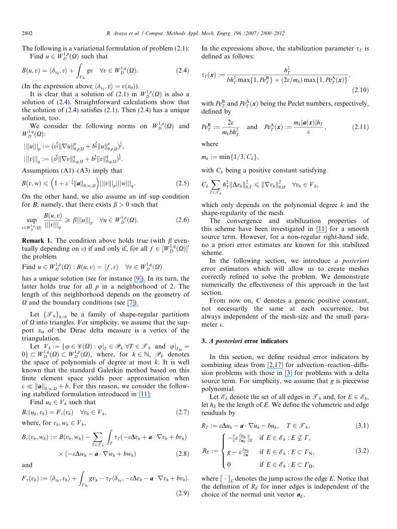
2802 R. Araya et al. / Comput. Methods Appl. Mech. Engrg. 196 (2007) 2800–2812

The following is a variational formulation of problem (2.1):Find u 2 W 1;p

D ðXÞ such that

Bðu; vÞ ¼ hdx0; vi þ

ZCN

gv 8v 2 W 1;qD ðXÞ: ð2:4Þ

(In the expression above hdx0; vi ¼ vðx0Þ).

It is clear that a solution of (2.1) in W 1;pD ðXÞ is also a

solution of (2.4). Straightforward calculations show thatthe solution of (2.4) satisfies (2.1). Then (2.4) has a uniquesolution, too.

We consider the following norms on W 1;pD ðXÞ and

W 1;qD ðXÞ:

jjjujjjp :¼ ðepqkrukp

0;p;X þ bpqkukp

0;p;XÞ1p;

jjjvjjjq :¼ ðeqpkrvkq

0;q;X þ bqpkvkq

0;q;XÞ1q:

Assumptions (A1)–(A3) imply that

Bðv;wÞ 6 1þ e�1qkak0;1;X

� �jjjvjjjpjjjwjjjq: ð2:5Þ

On the other hand, we also assume an inf–sup conditionfor B; namely, that there exists b > 0 such that

supv2W 1;q

D ðXÞ

Bðu; vÞjjjvjjjq

P bjjjujjjp 8u 2 W 1;pD ðXÞ: ð2:6Þ

Remark 1. The condition above holds true (with b even-tually depending on e) if and only if, for all f 2 ½W 1;q

D ðXÞ0

the problem

Find u 2 W 1;pD ðXÞ : Bðu; vÞ ¼ hf ; vi 8v 2 W 1;q

D ðXÞhas a unique solution (see for instance [9]). In its turn, thelatter holds true for all p in a neighborhood of 2. Thelength of this neighborhood depends on the geometry ofX and the boundary conditions (see [7]).

Let fThgh>0 be a family of shape-regular partitionsof X into triangles. For simplicity, we assume that the sup-port x0 of the Dirac delta measure is a vertex of thetriangulation.

Let V h :¼ fu 2 CðXÞ : ujT 2 Pk 8T 2Th and ujCD¼

0g � W 1;qD ðXÞ � W 1;p

D ðXÞ, where, for k 2 N, Pk denotesthe space of polynomials of degree at most k. It is wellknown that the standard Galerkin method based on thisfinite element space yields poor approximation whene� kak0;1;X þ b. For this reason, we consider the follow-ing stabilized formulation introduced in [11]:

Find uh 2 V h such that

Bsðuh; vhÞ ¼ F sðvhÞ 8vh 2 V h; ð2:7Þwhere, for vh;wh 2 V h,

Bsðvh;whÞ :¼ Bðvh;whÞ �X

T2Th

ZT

sT ð�eDvh þ a � rvh þ bvhÞ

� ð�eDwh � a � rwh þ bwhÞ ð2:8Þand

F sðvhÞ :¼ hdx0; vhi þ

ZCN

gvh � sT hdx0;�eDvh � a � rvh þ bvhi:

ð2:9Þ

In the expressions above, the stabilization parameter sT isdefined as follows:

sT ðxÞ :¼ h2T

bh2T maxf1; PeR

T g þ ð2e=mkÞmaxf1; PeAT ðxÞg

;

ð2:10Þ

with PeRT and PeA

T ðxÞ being the Peclet numbers, respectively,defined by

PeRT :¼ 2e

mkbh2T

and PeAT ðxÞ :¼ mkjaðxÞjhT

e; ð2:11Þ

where

mk :¼ minf1=3;Ckg;

with Ck being a positive constant satisfying

Ck

XT2Th

h2TkDvhk2

0;T 6 krvhk20;X 8vh 2 V h;

which only depends on the polynomial degree k and theshape-regularity of the mesh.

The convergence and stabilization properties ofthis scheme have been investigated in [11] for a smoothsource term. However, for a non-regular right-hand side,no a priori error estimates are known for this stabilizedscheme.

In the following section, we introduce a posteriori

error estimators which will allow us to create meshescorrectly refined to solve the problem. We demonstratenumerically the effectiveness of this approach in the lastsection.

From now on, C denotes a generic positive constant,not necessarily the same at each occurrence, butalways independent of the mesh-size and the small para-meter e.

3. A posteriori error indicators

In this section, we define residual error indicators bycombining ideas from [2,17] for advection–reaction–diffu-sion problems with those in [3] for problems with a deltasource term. For simplicity, we assume that g is piecewisepolynomial.

Let Eh denote the set of all edges in Th and, for E 2 Eh,let hE be the length of E. We define the volumetric and edgeresiduals by

RT :¼ eDuh � a � ruh � buh; T 2Th; ð3:1Þ

RE :¼

�se ouhonE

tE if E 2 Eh : E 6 C;

g � e ouhon

if E 2 Eh : E � CN;

0 if E 2 Eh : E � CD;

8>>><>>>: ð3:2Þ

where s � tE denotes the jump across the edge E. Notice thatthe definition of RE for inner edges is independent of thechoice of the normal unit vector nE.

R. Araya et al. / Comput. Methods Appl. Mech. Engrg. 196 (2007) 2800–2812 2803

These residuals are used to define an indicator of thelocal error as follows:

gT ;p :¼ap

T h�2p

qT þ ap

TkRT kp0;p;T þ

PE�oT

e�1qaEkREkp

0;p;E

� �1p

; �T 3 x0;

apTkRT kp

0;p;T þP

E�oTe�

1qaEkREkp

0;p;E

� �1p

; T 63 x0;

8>>>><>>>>:ð3:3Þ

where, for S ¼ T 2Th or S ¼ E 2 Eh,

aS :¼min hSe

�1p; b�

1p

n o; b > 0;

hSe�1

p; b ¼ 0:

8<: ð3:4Þ

In what follows we prove some technical lemmas.Let x0 :¼

SfT 2Th : x0 2 �T g and d :¼ distðx0; ox0Þ

(see Fig. 1). Notice that, because of the regularity of themesh, hT 6 Cd. Let wx0

be a smooth bubble functiondefined in X with support in x0 and satisfying:

0 6 wx0ðxÞ 6 1 8x 2 X; ð3:5Þ

wx0ðxÞ ¼ 1 8x 2 X : jx� x0j 6

d4; ð3:6Þ

wx0ðxÞ ¼ 0 8x 2 X : jx� x0jP

3d4; ð3:7Þ

jwx0jm;1;x0

6 Cd�m; m ¼ 1; 2: ð3:8Þ

Such a function can be easily obtained by convolution ofthe characteristic function of the set fx 2 X : jx� x0j <d=4g with a mollifier.

Lemma 2. Let �T 3 x0. Let wx0and x0 be defined as above.

Then

kwx0k0;q;E 6 Ch1=q

T ;

kwx0k0;q;T 6 Ch2=q

T ;

jjjwx0jjjq;T 6 Ca�1

T h2=qT :

Proof. Using (3.8) and the fact that hT 6 Cd, the definitionof j � jm;q yields

jwx0jm;q;E 6

ZEjDmwx0

ðxÞjq� �1=q

6 Cd�mh1=qT 6 Ch�mþ1=q

T :

Fig. 1. Domain x0 and support of wx0.

The same arguments yield

jwx0jm;q;T ¼

ZTjDmwx0

ðxÞjq� �1=q

6 Cd�mh2=qT 6 Ch�mþ2=q

T :

This inequality and the definition of jjj � jjjq allow us tocomplete the proof. h

Lemma 3. Given T 2Th, let sT be defined by (2.10). Then

the following bounds hold 8x 2 T :

esT ðxÞ 61

6h2

T ; jaðxÞjsT ðxÞ 61

2hT ; bsT ðxÞ 6 1:

Furthermore,

bsT ðxÞ 6 Cb1paT :

Proof. For the first estimate, we use (2.10) and (2.11) toobtain

esT ðxÞ 6eh2

T

bh2T maxf1; PeR

T g6

eh2T

bh2T PeR

T

6mk

2h2

T 61

6h2

T :

For the second one, if aðxÞ ¼ 0 there is nothing to prove;otherwise, by using (2.10) and (2.11) we have

jaðxÞjsT ðxÞ 6jaðxÞjmkh2

T

2e maxf1; PeAT ðxÞg

6jaðxÞjmkh2

T

2ePeAT ðxÞ

61

2hT :

For the third bound, (2.10) yields

bsT ðxÞ 61

maxf1; PeRT g6 1:

Moreover, from the first estimate of this lemma,bsT ðxÞ 6 Cbh2

T e�1, too. Hence, taking a weighted geometricmean of this and the third estimate, we have

bsT ðxÞ 6 Cb1ph

2pT e�

1p 6 CjXj

2pb

1p

hT

jXj

� �2p

e�1p 6 Cb

1phT e�

1p: �

Lemma 4. The following estimates hold for all wh 2 V h:

jwhjm;q;T 6 Ch�mT aT jjjwhjjjT ; m ¼ 1; 2:

Proof. The definition of the norm jjj � jjjq;T implies that

jwhj1;q;T 6 e�1pjjjwhjjjq;T ; ð3:9Þ

whereas, because of a standard scaling argument,

jwhj1;q;T 6 Ch�1T kwhk0;q;T 6 Ch�1

T b�1pjjjwhjjjq;T :

From these two inequalities we obtain

jwhj1;q;T 6 Ch�1T aT jjjwhjjjq;T : ð3:10Þ

On the other hand, another scaling argument and (3.10)yield

jwhj2;q;T 6 Ch�1T jwhj1;q;T 6 Ch�2

T aT jjjwhjjjq;T ;

which completes the proof. h

2804 R. Araya et al. / Comput. Methods Appl. Mech. Engrg. 196 (2007) 2800–2812

Lemma 5. The following estimates hold for all wh 2 V h:

jwhjm;1;T 6 Ch�m�2

qT aT jjjwhjjjT ; m ¼ 1; 2:

Proof. Standard scaling arguments yield

jwhjm;1;T 6 Ch�2

qT jwhjm;q;T ; m ¼ 0; 1; 2:

Finally, this estimate in addition to Lemma 4 complete theproof. h

Denote by IC : L2ðXÞ ! V h the Clement-like interpola-tion operator introduced in [4]. Given T 2Th, letexT :¼

[f�T 0 : T 0 2Th and �T 0 \ �T 6¼ ;g: ð3:11Þ

We prove several error estimates analogous to those inLemma 3.2 of [17].

Lemma 6. For all T 2Th, E � oT and v 2 W 1;qðexT Þ, thefollowing error estimates hold:

Fig. 2. Triangles T and T h.

kv� ICvk0;q;T 6 CaT jjjvjjjq;exT;

kv� ICvk0;q;E 6 Ce�1=ðpqÞa1=pE jjjvjjjq;exT

;

jjjICvjjjq;T 6 Cjjjvjjjq;exT:

Proof. The following error estimate for IC has been provedin [4]:

jv� ICvjl;q;T 6 Chk�lT jvjk;q;exT

8k; l : 0 6 l 6 k 6 1: ð3:12Þ

The first inequality of this lemma follows from this esti-mate with l ¼ 0 and k ¼ 0; 1. The following trace inequal-ity can be proved by standard scaling arguments:

kv� ICvk0;q;E

6 C h�1=qE kv� ICvk0;q;T þ kv� ICvk1=p

0;q;T jv� ICvj1=q1;q;T

� �:

Therefore, this inequality and the first inequality of thislemma yields

kv� ICvk0;q;E 6 C h�1=qE aT jjjvjjjq;exT

þ a1=pT jjjvjjjq;ex1=p

Tjvj1;q;ex1=q

T

� �6 C h�1=q

E a1=pT a1=q

T jjjvjjjq;exTþ a1=p

T e�1=ðpqÞjjjvjjjq;exT

� �6 Ce�1=ðpqÞa1=p

E jjjvjjjq;exT:

Finally, the third estimate of the lemma is also a conse-quence of (3.12) and the definition of k � k0;q;E. h

Lemma 7. For all v 2 W 1;qðexT Þ, there holds

kv� ICvk0;1;T 6 Ch1�2

qT e�

1pjjjvjjjq;exT

:

Proof. Let ILv denote the Lagrange interpolant of v, whichis well defined since v 2 W 1;qðexT Þ � CðexT Þ. The lemma fol-lows from interpolation error estimates and standard scal-ing arguments:

kv� ICvk0;1;T 6 kv� ILvk0;1;T þ kILv� ICvk0;1;T

6 C h1�2

qT jvj1;q;exT

þ h�2

qT kILv� ICvk0;q;T

h i6 C h

1�2q

T jvj1;q;exTþ h

�2q

T kv� ILvk0;q;exTþ kv� ICvk0;q;exT

� �h i6 Ch

1�2q

T e�1pjjjvjjjq;exT

: �

For each element T 2Th we define the element bubble

function wT by

wT :¼ 27Y

x2NðT Þkx;

where NðT Þ is the set of vertices of the element T and kx

denote the corresponding barycentric coordinates.In the sequel we will also use certain special bubble func-

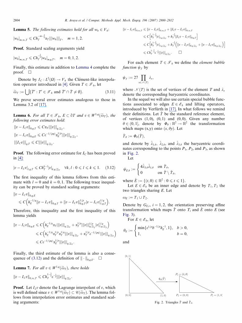
tions associated to edges E 2 Eh and lifting operators,introduced by Verfurth in [17]. In what follows we remindtheir definitions. Let T be the standard reference element,of vertices (1, 0), (0, 1) and (0, 0). Given any numberh 2 ð0; 1, denote by Uh : R2 ! R2 the transformationwhich maps (x,y) onto ðx; hyÞ. Let

T h :¼ UhðT Þ;

and denote by k1;h; k2;h, and k3;h the barycentric coordi-nates corresponding to the points P1, P2, and P3, as shownin Fig. 2.

Let

wE;h :¼ 4k3;hk1;h on T h;

0 on T n T h;

(where E :¼ fðt; 0Þ 2 R2 : 0 6 t 6 1g.

Let E 2 Eh be an inner edge and denote by T 1; T 2 thetwo triangles sharing E. Let

xE :¼ T 1 [ T 2:

Denote by GE;i, i ¼ 1; 2; the orientation preserving affinetransformation which maps T onto Ti and E onto E (seeFig. 3).

For E 2 Eh, let

hE :¼ minfe1=pb�1=ph�1E ; 1g; b > 0;

1; b ¼ 0;

(and

Fig. 3. Domain xE and affine transformations GE;i, i ¼ 1; 2:

Fig. 4. Domain T h.

R. Araya et al. / Comput. Methods Appl. Mech. Engrg. 196 (2007) 2800–2812 2805

wE :¼ wE;hE� G�1

E;i in T i; i ¼ 1; 2;

0 in X n xE:

(Let P :¼ fðx; 0Þ : x 2 Rg and Q : R2 ! P be the orthogo-nal projection from R2 onto P. We introduce the liftingoperator P E : PkðEÞ ! PkðT Þ by

P EðrÞ ¼ r � Q:

Let P E;T i : PkðEÞ ! PkðT iÞ defined by

P E;T iðrÞ ¼ P Eðr � GE;iÞ � G�1E;i ; i ¼ 1; 2:

Finally, we define a lifting operator for r 2 PkðEÞ by

P EðrÞ :¼P E;T 1ðrÞ in T 1;

P E;T 2ðrÞ in T 2:

�For E 2 Eh such that E � CN, the function wE and the lift-ing operator P E are similarly defined with the obviousmodifications.

Lemma 8. The following estimates hold for all v 2 Pk and

T 2Th:

kvk0;p;Tkvk0;q;T 6 Cðv;wT vÞT ;jjjwT vjjjq;T 6 Ca�1

T kvk0;q;T :

Furthermore, for all E 2 Eh and r 2 PkðEÞ, the following

estimates hold:

krk0;p;Ekrk0;q;E 6 Cðr;wErÞE;

kwEP EðrÞk0;q;xE6 Ce1=ðpqÞa1=q

E krk0;q;E;

jjjwEP EðrÞjjjq;xE6 Ce1=ðpqÞa�1=p

E krk0;q;E:

Proof. Scaling arguments show that

kvk0;r;T 6 Ch2r�1ðv;wT vÞ1=2

T with r ¼ p; q;

which yield the first inequality. The third inequality followsfrom a similar argument.

For the second one, using the fact that jrwT j 6 Ch�1T

and standard scaling arguments, we have

jjjvwT jjjq;T 6 C e1pkrðvwT Þk0;q;T þ b

1pkvwTk0;q;T

h i6 C e

1p kvrwTk0;q;T þ kwTrvk0;q;T

� �þ b

1pkvwTk0;q;T

h i6 C e

1ph�1

T kvk0;q;T þ b1pkvk0;q;T

h i6 C maxfe1

ph�1T ; b

1pgkvk0;q;T ¼ Ca�1

T kvk0;q;T :

The fourth inequality of the lemma follows from the defini-tion of k � k0;q;xE

and the fact that the size of the support ofwE in the orthogonal direction to E is bounded by ChEhE,with C only depending on the shape ratio of T (see Fig. 4):

kwEP EðrÞk0;q;xE¼Z

xE

jwEP EðrÞjq� �1=q

6C hEhE

ZEjwErjq

� �1=q

6Ce1pqa

1qEkrk0;q;E:

The last inequality of the lemma follows from the fact thatjrwEj 6 CðhEhEÞ�1 and standard scaling arguments:

jjjwEP EðrÞjjjq;xE6 C e

1pkrðwEP EðrÞÞk0;q;xE

þ b1pkwEP EðrÞk0;q;xE

h i6 C e

1p krwEP EðrÞk0;q;xE

þ kwErP EðrÞk0;q;xE

� �hþb

1pkwEP EðrÞk0;q;xE

i6 C e

1pðhEhT Þ�1kP EðrÞk0;q;xE

þ b1pkP EðrÞk0;q;xE

h i6 C maxfe1

ph�1T ; b

1pgkP EðrÞk0;q;xE

6 Ce1pqa�1

pE krk0;q;E;

where we have also used the fourth inequality of thislemma. h

Now we are in position to state the main theoreticalresult of the paper.

Theorem 9. Let B be defined by (2.3). Let p < 2 be such that

B satisfies (2.6) with a constant b > 0. Let u and uh be the

solutions of problems (2.4) and (2.7), respectively. Let gT ;p be

defined by (3.1)–(3.4) and, 8�T 3 x0, let g0;T be defined by

g0;T :¼ h2�p

pT e�

1p if bhp

T > e;

0 if bhpT 6 e:

(ð3:13Þ

Then, there exist constants C and C0, only depending on the

regularity of the mesh and the polynomial degree of the finiteelements, such that

jjju� uhjjjp 6Cb

XT2Th

gpT ;p þ

X�T3x0

gp0;T

!1p

ð3:14Þ

and

gT ;p 6 C0 1þ e�1qkak0;1;exT

� �jjju� uhjjjp;exT

8T 2Th;

where exT is defined by (3.11).

2806 R. Araya et al. / Comput. Methods Appl. Mech. Engrg. 196 (2007) 2800–2812

Proof. First, we write from (2.6),

bjjju� uhjjjp 6 supv2W 1;q

D ðXÞ

Bðu� uh; vÞjjjvjjjq

: ð3:15Þ

Now, consider an arbitrary v 2 W 1;qD ðXÞ with jjjvjjjq ¼ 1.

Obviously, we have

Bðu� uh; vÞ ¼ Bðu� uh; v� ICvÞ þ Bðu� uh; ICvÞ: ð3:16ÞElement-wise integration by parts yields

Bðu� uh;wÞ ¼ hdx0;wi þ

XT2Th

ðRT ;wÞT þXE2Eh

ðRE;wÞE

8w 2 W 1;qD ðXÞ: ð3:17Þ

Taking w ¼ v� ICv, invoking Holder’s inequality andLemmas 6 and 7, we have

Bðu� uh; v� ICvÞ

6 CX�T3x0

gp0;T þ

XT2Th

apTkRTkp

0;p;T þXE2Eh

e�1=qaEkREkp0;p;E

" #1p

6 CX�T3x0

gp0;T þ

XT2Th

gpT ;p

" #1p

: ð3:18Þ

For the second term in the right-hand side of (3.16), from(2.3), (2.4), (2.7)–(2.9), we have

Bðu� uh;whÞ ¼ sT 0hdx0

;�eDwh � a � rwh þ bwhi

�X

T2Th

ZT

sT ðRT ;�eDwh � a � rwh þ bwhÞ:

Next, from Lemmas 3 and 4, straightforward computationslead toZ

TsT ðRT ;�eDwh � a � rwh þ bwhÞ 6 CaTkRTk0;p;T jjjwhjjjq;T ;

whereas from Lemmas 3 and 5 we have

sT 0hdx0

;�eDwh � a � rwh þ bwhi 6 CaT 0h�2

qT 0jjjwhjjjq;T 0

:

Finally, we replace wh by ICv and use Lemma 6 to obtain

Bðu� uh; ICvÞ 6 C aT 0h�2

qT 0jjjvjjjq;exT0

þX

T2Th

aT kRT k0;p;T jjjvjjjq;exTÞ:

From the regularity of the mesh and the fact that jjjvjjjq ¼ 1there holds

Bðu� uh; ICvÞ 6 CX�T3x0

apT h�2p

qT þ

XT2Th

apTkRTkp

0;T

" #1p

6 CX

T2Th

gpT ;p

" #1p

: ð3:19Þ

Thus, the first estimate of the theorem is a consequence of(3.15), (3.18) and (3.19).

To derive the other estimate of the theorem, we consideran arbitrary T 2Th. First, we take w ¼ wT RT in (3.17),and we have

Bðu� uh;wT RT Þ ¼ ðRT ;wT RT ÞT : ð3:20ÞUsing Lemma 8, (3.20), and Lemma 8 again, we have

kRTk0;p;TkRTk0;q;T

6 CðRT ;wT RT ÞT ¼ CBðu� uh;wT RT Þ

6 C 1þ e�1qkak0;1;T

� �jjju� uhjjjp;T jjjwT RT jjjq;T

6 C 1þ e�1qkak0;1;T

� �jjju� uhjjjp;T a�1

T kRTk0;q;T :

Hence,

aTkRTk0;p;T 6 C 1þ e�1qkak0;1;T

� �jjju� uhjjjp;T : ð3:21Þ

On the other hand, taking w ¼ wEP EðREÞ in (3.17) weobtain

ðRE;wÞE ¼ Bðu� uh;wÞ �XT2xE

ðRT ;wÞT

6 1þ e�1qkak0;1;xE

� �jjju� uhjjjp;xE

jjjwjjjq;xE

þXT2xE

kRTk0;p;Tkwk0;q;T :

Now, from Lemma 8,

kREk0;p;EkREk0;q;E 6 C 1þ e1qkak0;1;xE

� �jjju� uhjjjp;xE

e1pqa�1

pE

"

kREk0;q;E þXT2xE

kRTk0;p;T e1=ðpqÞa1=qE kREk0;q;E

#and, multiplying by e�1=ðpqÞa1=p

E , we obtain

e�1=ðpqÞa1=pE kREk0;p;E 6 C 1þ e

1qkak0;1;xE

� �jjju� uhjjjp;T

XT2xE

aTkRTk0;p;T

" #:

ð3:22ÞFinally, taking w ¼ wx0

in (3.17), we have

hdx0;wx0i ¼ Bðu� uh;wx0

Þ �X

T2Th

ðRT ;wx0ÞT �

XE2Eh

ðRE;wx0ÞE:

Using the properties of wx0from Lemma 2, (2.5), and Hol-

der’s inequality, we obtain

1 6 1þ e�1qkak0;1;T

� �jjju� uhjjjp;T jjjwx0

jjj0;q;TþXT2xT

kRTk0;p;Tkwx0k0;q;T þ

XE2Eh

kREk0;p;Ekwx0k0;q;E

6 C 1þ e�1qkak0;1;T

� �jjju� uhjjjp;T h2=q

T a�1T

"

þXT2xT

kRTk0;p;T h2=qT þ

XE2Eh

kREk0;p;Eh1=qT

#:

Thus,

h�2=qT 0

aT 06 C 1þ e�

1qkak0;1;T

� �jjju� uhjjj0;p;T

"

þXT2xT

aTkRTk0;p;T þXE2Eh

e�1pqa

1pEkREk0;p;E

#; ð3:23Þ

101 102 103 104 10510—1

100

101

102

103

104

d.o.f

erro

r

Slope —1/2Exact errorηη*

Fig. 7. Test 1. Estimators g and g�, and exact W 1;pD ðXÞ-norm error curves.

R. Araya et al. / Comput. Methods Appl. Mech. Engrg. 196 (2007) 2800–2812 2807

where we have used the fact that h�1

qT aE 6 e�

1pqa

1pE and the reg-

ularity of the mesh.Thus, the second estimate of the theorem follows from

(3.21)–(3.23), and the definition of the estimator gT ;p, andwe conclude the proof. h

Remark 10. As mentioned above, the constant b in theestimate (3.14) might depend on e. In such case, thisestimate would not be accurate. However, ð

PT2Th

gpT ;pþP

�T3x0gp

0;T Þ1p can be used as an error indicator to

determine where to refine the mesh in an adaptiveprocess.

Remark 11. In absence of reaction, b ¼ 0 and, accordingto (3.13), g0;T ¼ 0, too. Consequently, the indicator

ðP

T2Thgp

T ;pÞ1p is actually equivalent to the error for the

advection–diffusion problem.

Fig. 5. Test 1. Meshes and computed solutions.

Fig. 6. Test 1. Successive zooms of the final adapted mesh.

2808 R. Araya et al. / Comput. Methods Appl. Mech. Engrg. 196 (2007) 2800–2812

4. Numerical experiments

In this section, we report several numerical experimentswhich allow us to assess the performance of an h-adaptivemesh-refinement strategy based on the error indicatorsanalyzed in the previous section.

The adaptive procedure consists in solving problem (2.7)on a sequence of meshes up to finally attain a solution withan estimated error within a prescribed tolerance. With thispurpose, we initiate the process with a quasi-uniform mesh

Table 1Effectivity indices

dof g=jjju� uhjjjp g�=jjju� uhjjjp21 0.0379 10.95841 0.0972 6.925573 1.4662 4.3105

161 3.0792 3.0792321 3.4418 3.4418589 3.3195 3.3195

1251 3.6453 3.64532339 3.8643 3.86435125 4.1035 4.10359695 4.0894 4.0894

17417 4.1094 4.1094

Fig. 8. Test 2. Boundary conditions.

Fig. 9. Test 2. Meshes obtaine

and, at each step, a new mesh better adapted to the solu-tion of problem (2.4) must be created. This is done bycomputing the local error estimators gT ;p for all T in the‘old’ mesh Th, and refining those elements T withgT ;p P l maxfgT ;p : T 2Thg, where l 2 ð0; 1Þ is a pre-scribed parameter. In all our experiments we have chosenl ¼ 1

2and p ¼ 1:5. The last choice guarantees that (2.6)

holds true. Indeed, according to [7], (2.6) is valid forp 2 ð1;1Þ in the first two cases and for p 2 ð4

3; 4Þ in the

third one. To refine the meshes we have used the red–green–blue strategy described in [16].

4.1. Test 1: a diffusion–reaction problem

For the first test we consider the problem

�eDuþ bu ¼ dx0: ð4:1Þ

A fundamental solution of (4.1) is given by

uðxÞ :¼ 1

4ieH ð1Þ0

ffiffiffibe

rijx� x0j

!; ð4:2Þ

where H ð1Þ0 denotes the Hankel function of order zero (see[1]). The test consists of solving problem (4.1) withx0 ¼ ð0; 0Þ on the square X :¼ ð�1; 1Þ � ð�1; 1Þ, e ¼ 10�4

and b ¼ 1. We choose a Dirichlet boundary condition suchthat the exact solution is given by the real part of (4.2).

We report the results obtained for the adaptive processwith gT ;p as estimator of the error. Fig. 5 shows some ofthe successively refined meshes created in the adaptive pro-cess and the corresponding computed solutions. The itera-tion number and the number of degrees of freedom (dof) ofeach mesh are also reported in this figure.

Fig. 6 shows successive zooms of the final adapted mesharound x0. The second square corresponds to the whiteinner square in the first one amplified 10 times aroundx0, and so on.

d by the adaptive process.

R. Araya et al. / Comput. Methods Appl. Mech. Engrg. 196 (2007) 2800–2812 2809

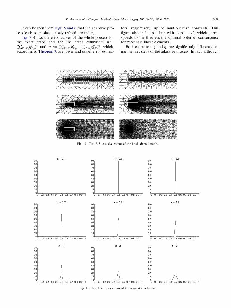
It can be seen from Figs. 5 and 6 that the adaptive pro-cess leads to meshes densely refined around x0.

Fig. 7 shows the error curves of the whole process forthe exact error and for the error estimators g :¼ðP

T2Thgp

T ;pÞ1p and g� :¼ ð

PT2Th

gpT ;p þ

P�T3x0

gp0;T Þ

1p, which,

according to Theorem 9, are lower and upper error estima-

Fig. 10. Test 2. Successive zoom

0 0.1 0.2 0.3 0.4 0.5 0.6 0.7 0.8 0.9 10

10

20

30

40

50

60

70

80

90x = 0.4

0 0.1 0.2 0.3 0.4 0.5 0.6 0.7 0.8 0.9 10

10

20

30

40

50

60

70

80

90x = 0.7

0 0.1 0.2 0.3 0.4 0.5 0.6 0.7 0.8 0.9 10

10

20

30

40

50

60

70

80

90x =1

0 0.1 0.2 0.3 0.4 0.50

10

20

30

40

50

60

70

80

90x = 0

0 0.1 0.2 0.3 0.4 0.50

10

20

30

40

50

60

70

80

90x = 0

0 0.1 0.2 0.3 0.4 0.50

10

20

30

40

50

60

70

80

90x =2

Fig. 11. Test 2. Cross sections

tors, respectively, up to multiplicative constants. Thisfigure also includes a line with slope �1/2, which corre-sponds to the theoretically optimal order of convergencefor piecewise linear elements.

Both estimators g and g� are significantly different dur-ing the first steps of the adaptive process. In fact, although

s of the final adapted mesh.

0.6 0.7 0.8 0.9 1

.5

0.6 0.7 0.8 0.9 1

.8

0.6 0.7 0.8 0.9 1

0 0.1 0.2 0.3 0.4 0.5 0.6 0.7 0.8 0.9 10

10

20

30

40

50

60

70

80

90x = 0.6

0 0.1 0.2 0.3 0.4 0.5 0.6 0.7 0.8 0.9 10

10

20

30

40

50

60

70

80

90x = 0.9

0 0.1 0.2 0.3 0.4 0.5 0.6 0.7 0.8 0.9 10

10

20

30

40

50

60

70

80

90x =3

of the computed solution.

2810 R. Araya et al. / Comput. Methods Appl. Mech. Engrg. 196 (2007) 2800–2812

they only differ in the triangles �T 3 x0, the error concen-trates on these elements. This is the reason why the differ-ence between g and g� is so pronounced.

101 102 103 104 105100

101

102

d.o.f

erro

r

Slope —0.4η

Fig. 12. Test 2. Error curves for the estimator g.

Fig. 13. Test 3. Initial mesh and

Fig. 14. Test 3. V

However both estimators are equally good to guide theadaptive process. Indeed, exactly the same meshes appear ifg� is used instead of g in this test. Once the elements T

around x0 are sufficiently refined so that bhpT 6 e, according

to the definition of g0;T , both estimators coincide. It can beseen from Fig. 7 that this happens in this test after around10 steps.

The error curves show that, at the final stage, the adap-tive process yields an optimal order of convergence: theexact and estimated error curves have both approximatelythe same optimal slope �1/2.

Finally, we report in Table 1 the effectivity indices ofboth indicators.

4.2. Test 2: an advection–diffusion problem

The second test consists of solving the problem

�eDuþ a � ru ¼ dx0;

with x0 ¼ ð0:5; 0:5Þ, X :¼ ð0; 3Þ � ð0; 1Þ, e ¼ 10�4, anda ¼ ð1; 0Þ. We choose boundary conditions as shown inFig. 8.

location of the source point.

elocity field a.

R. Araya et al. / Comput. Methods Appl. Mech. Engrg. 196 (2007) 2800–2812 2811

Let us recall that in this case (b ¼ 0), both estimators gand g� coincide.

Fig. 9 shows some of the successively refined meshes cre-ated in the adaptive process for gT ;p, with p ¼ 1:5.

Fig. 10 shows successive zooms around x0 of the finaladapted mesh. It can be seen from Figs. 9 and 10 thatthe adaptive process leads to meshes refined around both,x0 and the interior layer.

Fig. 11 shows several cross sections with vertical planesx ¼ constant. It can be seen that the numerical results pres-ent no spurious oscillations in the layer zone.

Fig. 12 shows the error curves of the whole process forthe estimated errors. A computed order of convergenceof approximately �0.4 was obtained by means of a leastsquares fitting.

4.3. Test 3: application to the Bıo-Bıo river

Our last test consists of an application of the describedmethodology to a realistic scenario: a water quality model

Fig. 16. Test 3. Isovalues of

Fig. 15. Test 3.

for Bıo-Bıo river in Chile. With this purpose we havesolved the advection–diffusion–reaction equation (2.1)which describes transport and degradation of pollutantsarising from a point source. Fig. 13 shows the geometryof the domain, which correspond to a section of Bıo-Bıoriver and two tributaries. It also shows the initial used mesh(773 nodes) and the source point at one of the tributaries.

Fig. 14 shows the velocity field a; the average speedis 0.02 km/s. We have used e ¼ 10�6 km2=s andb ¼ 10�3 s�1. We have taken the following boundary condi-tions: u ¼ 0 on the three inflow parts of the boundary andou=on ¼ 0 on the banks and the outflow boundary.

Fig. 15 shows the final mesh (19,884 nodes) after 60steps of the adaptive process. It can be seen that the meshis well aligned with the interior layer.

Fig. 16 shows the isovalues of the computed solution inthe range 10�1–103 on the final adapted mesh. It can beclearly seen that the combined effect of the stabilizationand the adaptive process allow us to identify the interiorlayer and get rid of any spurious oscillation.

the computed solution.

Final mesh.

2812 R. Araya et al. / Comput. Methods Appl. Mech. Engrg. 196 (2007) 2800–2812

5. Conclusions

An adaptive finite element scheme for the advection–reaction–diffusion equation with a Dirac delta source termhas been introduced. This scheme is based on a stabilizedfinite element method combined with a residual error esti-mator. In spite of the fact that the used stabilization tech-nique was originally introduced only for regular right-handsides, our numerical experiments show that the scheme isconvergent in our case, too. On the other hand, the estima-tor is shown to be reliable and efficient in that global upperand local lower error estimates are proved, although withconstants eventually depending on the diffusion parameter.

Several numerical experiments are reported. All of themshow the effectiveness of this scheme to capture the layersvery sharply and without significant oscillations.

Acknowledgment

This work was done in the framework of FONDEF re-search project D001135.

References

[1] M. Abramowitz, I.A. Stegun, Handbook of Mathematical Functionswith Formulas, Graphs, and Mathematical Tables, Dover publica-tions Inc., New York, 1970.

[2] R. Araya, E. Behrens, R. Rodrıguez, An adaptive stabilized finiteelement scheme for the advection–reaction–diffusion equation, Appl.Numer. Math. 54 (3–4) (2005) 491–503.

[3] R. Araya, E. Behrens, R. Rodrıguez, A posteriori error estimates forelliptic problems with dirac delta source terms, Numer. Math. 105 (2)(2006) 193–216.

[4] C. Bernardi, V. Girault, A local regularization operator for triangularand quadrilateral finite elements, SIAM J. Numer. Anal. 35 (5) (1998)1893–1916.

[5] F. Brezzi, D. Marini, A. Russo, Applications of the pseudo residual-free bubbles to the stabilization of convection–diffusion problems,Comput. Methods Appl. Mech. Engrg. 166 (1-2) (1998) 51–63.

[6] A.N. Brooks, T.J.R. Hughes, Streamline upwind/Petrov–Galerkinformulations for convection dominated flows with particular empha-sis on the incompressible Navier–Stokes equations, Comput. Meth-ods Appl. Mech. Engrg. 32 (1–3) (1982) 199–259.

[7] M. Dauge, Elliptic Boundary Value Problems on Corner Domains,Lecture Notes in Mathematics, vol. 1341, Springer, Berlin, 1988.

[8] J. Douglas, J.P. Wang, An absolutely stabilized finite element methodfor the Stokes problem, Math. Comp. 52 (186) (1989) 495–508.

[9] A. Ern, J.L. Guermond, Theory and Practice of Finite Elements,Applied Mathematical Sciences, vol. 159, Springer, New York, 2004.

[10] L.P. Franca, S.L. Frey, T.J.R. Hughes, Stabilized finite elementmethods. I. Application to the advective–diffusive model, Comput.Methods Appl. Mech. Engrg. 95 (2) (1992) 253–276.

[11] L.P. Franca, F. Valentin, On an improved unusual stabilized finiteelement method for the advective–reactive–diffusive equation, Com-put. Methods Appl. Mech. Engrg. 190 (13–14) (2000) 1785–1800.

[12] P. Grisvard, Elliptic Problems in Nonsmooth Domains, Monographsand Studies in Mathematics, vol. 24, Pitman (Advanced PublishingProgram), Boston, MA, 1985.

[13] T. Knopp, G. Lube, G. Rapin, Stabilized finite element methods withshock capturing for advection–diffusion problems, Comput. MethodsAppl. Mech. Engrg. 191 (27–28) (2002) 2997–3013.

[14] H.G. Roos, M. Stynes, L. Tobiska, Numerical Methods for Singu-larly Perturbed Differential Equations, Springer Series in Computa-tional Mathematics, vol. 24, Springer, Berlin, 1996.

[15] G. Sangalli, A robust a posteriori estimator for the residual-freebubbles method applied to advection–diffusion problems, Numer.Math. 89 (2) (2001) 379–399.

[16] R. Verfurth, A Review of a posteriori Error Estimation and AdaptiveMesh-refinement Techniques, Wiley, New York, 1996.

[17] R. Verfurth, A posteriori error estimators for convection–diffusionequations, Numer. Math. 80 (4) (1998) 641–663.

[18] R. Verfurth, Robust a posteriori error estimators for a singularlyperturbed reaction–diffusion equation, Numer. Math. 78 (3) (1998)479–493.

[19] S. Wang, An a posteriori error estimate for finite element approx-imations of a singularly perturbed advection–diffusion problem, J.Comput. Appl. Math. 87 (2) (1997) 227–242.