Analytical solutions of one-dimensional advection–diffusion equation with variable coefficients in

a finite domain

Atul Kumar, Dilip Kumar Jaiswal and Naveen Kumar∗

Department of Mathematics, Faculty of Science, Banaras Hindu University, Varanasi 221 005, India.∗e-mail: naveen@bhu.ac.in nks−1953@yahoo.co.in

Analytical solutions are obtained for one-dimensional advection–diffusion equation with variablecoefficients in a longitudinal finite initially solute free domain, for two dispersion problems. In thefirst one, temporally dependent solute dispersion along uniform flow in homogeneous domain isstudied. In the second problem the velocity is considered spatially dependent due to the inhomo-geneity of the domain and the dispersion is considered proportional to the square of the velocity.The velocity is linearly interpolated to represent small increase in it along the finite domain. Thisanalytical solution is compared with the numerical solution in case the dispersion is proportionalto the same linearly interpolated velocity. The input condition is considered continuous of uniformand of increasing nature both. The analytical solutions are obtained by using Laplace transforma-tion technique. In that process new independent space and time variables have been introduced.The effects of the dependency of dispersion with time and the inhomogeneity of the domain on thesolute transport are studied separately with the help of graphs.

1. Introduction

Advection–diffusion equation describes the solutetransport due to combined effect of diffusion andconvection in a medium. It is a partial differen-tial equation of parabolic type, derived on theprinciple of conservation of mass using Fick’s law.Due to the growing surface and subsurface hydro-environment degradation and the air pollution,the advection–diffusion equation has drawn signif-icant attention of hydrologists, civil engineers andmathematical modelers. Its analytical/numericalsolutions along with an initial condition and twoboundary conditions help to understand the con-taminant or pollutant concentration distributionbehaviour through an open medium like air, rivers,lakes and porous medium like aquifer, on the basisof which remedial processes to reduce or eliminatethe damages may be enforced. It has wide applica-tions in other disciplines too, like soil physics,

petroleum engineering, chemical engineering andbiosciences.

In the initial works while obtaining the ana-lytical solutions of dispersion problems in idealconditions, the basic approach was to reduce theadvection–diffusion equation into a diffusion equa-tion by eliminating the convective term(s). It wasdone either by introducing moving co-ordinates(Ogata and Banks 1961; Harleman and Rumer1963; Bear 1972; Guvanasen and Volker 1983;Aral and Liao 1996; Marshal et al 1996) or byintroducing another dependent variable (Banksand Ali 1964; Ogata 1970; Lai and Jurinak1971; Marino 1974 and Al-Niami and Rushton1977). Then Laplace transformation techniquehas been used to get desired solutions. In addi-tion to this method, Hankel transform method,Aris moment method, perturbation approach,method using Green’s function, superpositionmethod have also been used to get the analytical

Keywords. Advection; diffusion; dispersion; aquifer; groundwater.

J. Earth Syst. Sci. 118, No. 5, October 2009, pp. 539–549© Printed in India. 539

540 Atul Kumar et al

solutions of the advection–diffusion equations inone, two and three dimensions. But Laplace trans-formation technique has been commonly usedbecause of being simpler than other methods andthe analytical solutions using this method beingmore reliable in verifying the numerical solutionsin terms of the accuracy and the stability.

Most of the works included the effects of adsorp-tion, first order decay, zero order productionon the concentration attenuation as the soluteis transported down the stream. Such solutionshave been compiled (van Genuchten and Alves1982 and Lindstrom and Boersma 1989). Comingnearer to real problems layered porous mediumwas considered (Shamir and Harleman 1967), inho-mogeneity of the porous medium was definedas a function of distance variable (Lin 1977),and non-linear adsorption has been considered(Liej et al 1993). Using the direct relationshipbetween dispersion coefficient and velocity throughporous medium (Ebach and White 1958), unsteadyflow through porous medium has been consideredto obtain the analytical solutions (Banks andJerasate 1962; Hunt 1978 and Kumar 1983). Someone-dimensional analytical solutions have beengiven (Tracy 1995) by transforming the non-linearadvection–diffusion equation into a linear one forspecific forms of the moisture content vs. pressurehead and relative hydraulic conductivity vs. pres-sure head curves which allow both two-dimensionaland three-dimensional solutions to be derived.A method has been given to solve the trans-port equations for a kinetically adsorbing solute ina porous medium with spatially varying velocityfield and dispersion coefficients (Van Kooten 1996).A methodology was presented (Manoranjan andStauffer 1996) which enables to construct a closedform exact solution for transport with Langmuirsorption under nonequilibrium conditions withoutmaking any kind of restrictive a priori assump-tions. A stochastic model for one-dimensional virustransport in homogeneous, saturated, semi-infiniteporous media was developed (Chrysikopoulos andSim 1996), the model accounts for first-orderinactivation of liquid-phase, adsorbed viruses withdifferent inactivation rate constants, and timedependent distribution coefficient.

Later it has been shown that some large sub-surface formations exhibit variable dispersivityproperties, either as a function of time or as a func-tion of distance (Matheron and deMarsily 1980;Sposito et al 1986; Gelhar et al 1992). Analyticalsolutions were developed for describing the trans-port of dissolved substances in heterogeneous semi-infinite porous media with a distance dependentdispersion of exponential nature along the uni-form flow (Yates 1990, 1992). The work of Yateswas extended (Logan and Zlotnik 1995 and Logan

1996) by including the adsorption and decay effectsand by studying their interaction with the inhomo-geneity caused by scale-dependent dispersion alonguniform flow for periodic input condition. One-dimensional analytical solutions were presented forthe advection–diffusion equation for solute disper-sion, being proportional to the square of velocityand velocity proportional to the position variable(Zoppou and Knight 1997). Time dependent dis-persion along uniform flow has been considered(Aral and Liao 1996) to solve two-dimensionaladvection–diffusion equation. An analytical solu-tion has been obtained for two dimensional steadystate mass transports in a trapezoidal embank-ment in a spatially varying velocity field through itsreplacement with a hydrologically equivalent rect-angular embankment (Tartakovsky and Federico1997).

The temporal moment solution for one dimen-sional advective-dispersive solute transport withlinear equilibrium sorption and first order degra-dation for time pulse sources has been appliedto analyze soil column experimental data (Panget al 2003). An analytical approach was developedfor nonequilibrium transport of reactive solutesin the unsaturated zone during an infiltration–redistribution cycle (Severino and Indelman 2004).The solute is transported by advection and obeyslinear kinetics. Analytical solutions were pre-sented for solute transport in rivers including theeffects of transient storage and first order decay(Smedt 2006). Pore flow velocity was assumedto be a nondivergence – free, unsteady and non-stationary random function of space and time forground water contaminant transport in a hetero-geneous media (Sirin 2006). A two-dimensionalsemi-analytical solution was presented to analyzestream–aquifer interactions in a coastal aquiferwhere groundwater level responds to tidal effects(Kim et al 2007).

In the present paper analytical solutions areobtained for two solute dispersion problems in alongitudinal finite domain, organized in sections 2and 3, respectively. In the first problem time depen-dent solute dispersion of increasing or decreasingnature along a uniform flow through a homo-geneous domain is studied. In the second problemthe medium is considered inhomogeneous hencethe velocity is considered dependent on positionvariable. The velocity is linearly interpolated inposition variable which represents a small increasein the velocity from one end to the other end ofthe domain. This expression contains a parameterto represent a change in inhomogeneity from onemedium to other medium. Dispersion is assumedproportional to square of velocity. In each problemthe domain is initially solute free. The input condi-tion is of uniform and varying nature, respectively.

Analytical solutions of advection–diffusion equation 541

Numerical solution has also been obtained for thecase in which dispersion varies linearly with velo-city and has been compared with the analyticalsolution obtained in the former case.

2. Temporally dependent dispersionalong uniform flow

2.1 Uniform continuous input

Advection–diffusion equation in one dimensionwith variable coefficients is:

∂C

∂t=

∂

∂x

(D(x, t)

∂C

∂x− u(x, t)C

), (1)

where C represents the solute concentration atposition x along the longitudinal direction at timet, D is the solute dispersion, if it is independent ofposition and time, is called dispersion coefficient,and u is the medium’s flow velocity. To study thetemporally dependent solute dispersion of a uni-form input concentration of continuous nature inan initially solute free finite domain, we consider

D(x, t) = D0f(mt) and u(x, t) = u0, (2)

where m is a coefficient whose dimension is inverseof that of the time variable. Thus f(mt) isan expression in non-dimensional variable (mt).The expressions of f(mt) are chosen such thatf(mt) = 1 for m = 0 or t = 0. The former caserepresents the uniform solute dispersion andthe latter case represents the initial dispersion.The coefficients D0 and u0 in equation (2) may bedefined as initial dispersion coefficient and uniformflow velocity, respectively. Thus the partial differ-ential equation (1) along with initial condition andboundary conditions may be written as:

∂C

∂t= D0f(mt)

∂2C

∂x2− u0

∂C

∂x, (3)

C(x, t) = 0, 0 ≤ x ≤ L, t = 0, (4)

C(x, t) = C0, x = 0, t > 0, (5)

∂C(x, t)∂x

= 0, x = L, t ≥ 0, (6)

where the input condition is assumed at the originand a second type or flux type homogeneous

condition is assumed at the other end x = L, of thedomain. C0 is a reference concentration.

To use the Laplace transform technique con-veniently, it is necessary to bring the time depen-dent coefficient in differential equation (3) on theleft hand side. For this purpose we introduce a newindependent variable by a transformation

X =∫

dx

f(mt)or

dX

dx=

1f(mt)

. (7)

As mt is a non-dimensional term so the dimensionof X will be that x hence is referred to as a newspace variable, a moving co-ordinate, though it isdifferent from those considered in the referencescited at the outset of the first section. The initialand boundary value problem in new space variablemay be expressed as:

f(mt)∂C

∂t= D0

∂2C

∂X2− u0

∂C

∂X, (8)

C(X, t) = 0, 0 ≤ X ≤ X0,

t = 0; X0 =L

f(mt), (9)

C(X, t) = C0, X = 0, t > 0, (10)

∂C(X, t)∂X

= 0, X = X0, t ≥ 0. (11)

To get rid of the time dependent coeffi-cient following transformation (Crank 1975) isused:

T =

t∫0

dt

f(mt). (12)

The dimension of T will be that of the variable tso it is referred to as a new time variable. Furtherit should also be ensured while choosing f(mt)that T = 0 at t = 0 so that the nature of ini-tial condition does not change in the new timedomain. The initial and boundary value problem(equations 8–11) may be expressed in new timevariable as:

∂C

∂T= D0

∂2C

∂X2− u0

∂C

∂X, (13)

C(X,T ) = 0, 0 ≤ X ≤ X0,

T = 0; X0 =L

f(mt), (14)

542 Atul Kumar et al

C(X,T ) = C0, X = 0, T > 0, (15)

∂C(X,T )∂X

= 0, X = X0, T ≥ 0. (16)

Now the initial and boundary value problem(equations 13–16) in the (X,T ) domain becomessimilar to that of Cleary and Adrian (1973) in(x, t), quoted as problem A3 (van Genuchten andAlves 1982), hence or otherwise using Laplacetransformation technique, the desired analyticalsolution may be written as follows:

C(X,T ) = C0A(X,T ), (17)

where

A(X,T )

=12

erfc(

X − u0T

2√

D0T

)

+12

exp(

u0X

D0

)erfc

(X + u0T

2√

D0T

)

+12

[2 +

u0(2X0 − X)D0

+u2

0T

D0

]

× exp(

u0X0

D0

)erfc

((2X0 − X) + u0T

2√

D0T

)

−(

u20T

πD0

)1/2

exp[u0X0

D0

− (2X0−X+u0T )2

4D0T

],

X = x/f(mt), X0 = L/f(mt) and T may beobtained from transformation (equation 12).

2.2 Input condition of increasing nature

The source of input concentration may increasewith time due to variety of reasons. One way torepresent such a condition is to consider a factorC0F (t) on right hand side of the input condi-tion (equation 5) where F (t) may be an increasingfunction. But this type of situation may also bedescribed by a mixed type or third type conditionwritten as follows:

−D(x, t)∂C

∂x+ u(x, t)C = u0C0 at x = 0, t > 0.

(18)

Using equations (2), (7) and (12) the above condi-tion may be written in (X,T ) domain as:

−D0

∂C

∂X+ u0C = u0C0 at X = 0, T > 0. (19)

Now the initial and boundary value problemcomposed of advection–diffusion equation (13),initial condition (14), input condition (19) andsecond boundary condition (16), in the (X,T )domain becomes similar to that of Bastian andLapidus (1956) and Brenner (1962) in (x, t)domain, quoted as the problem A4 (van Genuchtenand Alves 1982) hence or otherwise using Laplacetransformation technique, the desired analyticalsolution may be written as follows:

C(X,T ) = C0A(X,T ) (20)

where

A(X,T )

=12

erfc(

X − u0T

2√

D0T

)+

(u2

0T

πD0

)1/2

× exp[−(X + u0T )2

4D0T

]− 1

2

(1 +

u0X

D0

+u2

0T

D0

)

× exp(

u0X

D0

)erfc

(X + u0T

2√

D0T

)

+(

4u0T

πD0

)1/2 [1 +

u0

4D0

(2X0 − X + u0T )]

× exp[u0X0

D0

− (2X0 − X + u0T )4D0T

]− u0

D0

×[(2X0−X)+

3u0T

2+

u0

4D0

(2X0−X+u0T )2]

× exp(

u0X0

D0

)erfc

((2X0 − X) + u0T

2√

D0T

),

X = x/f(mt), X0 = L/f(mt) and T may beobtained from transformation (12).

Analytical solutions of advection–diffusion equation 543

3. Spatially dependent dispersion alongnon-uniform flow

3.1 Uniform input

Though inhomogeneity of porous domain wasdefined by scale dependent dispersion and flowthrough the medium has been considered uniform(Yates 1992; Logan 1996) but the flow velocitymay also depend upon position variable in casethe domain is inhomogeneous. Zoppou and Knight(1997) have considered the velocity as u = βx,and the solute dispersion proportional to square ofvelocity, i.e., as D = αx2; in a semi-infinite domainx0 ≤ x < ∞. But these expressions do not reflectreal variations due to inhomogeneity of the mediumbecause as x → ∞, dispersion and velocity alsobecome too large. In fact the variation in velocitydue to inhomogeneity should be small so that thevelocity at each position satisfies the Darcy’s law incase the medium is porous or satisfies the laminarcondition of the flow in a non-porous medium, anessential condition for the velocity parameter, uin the advection–diffusion equation. This factor istaken care of in the present work and velocity islinearly interpolated in position variable such thatit increases from a value u0 at x = 0 to a value(1 + b)u0 at x = L, where b may be a real constant.Thus

u(x, t) = u0(1 + ax), (21)

where a = b/L, is the parameter accounting for theinhomogeneity of the medium. It should be smallso that the increase in velocity is of small order.Solute dispersion is assumed proportional to squareof the velocity so we consider

D(x, t) = D0(1 + ax)2. (22)

As ax is a non-dimensional term hence D0 andu0 are dispersion coefficient and velocity, respec-tively at the origin (x = 0) of the medium. Thedomain is assumed initially solute free. An inputconcentration is assumed at the origin and aflux type homogeneous condition is assumed atthe other end of the domain. Now to solveadvection–diffusion equation (1) for the expres-sions in (21) and (22) along with the conditions(4–6) we introduce a new space variable, X by atransformation

X = −∫

dx

(1 + ax)2=

1a(1 + ax)

, (23)

in terms of which the advection–diffusionequation (1) assumes the form

∂C

∂t= a2D0X

2 ∂2C

∂X2+ au0X

∂C

∂X− au0C. (24)

It is further reduced into a partial differentialequation with constant coefficients by using atransformation

Z = − log aX = log(1 + ax). (25)

Ultimately we get the present initial and boundaryvalue dispersion problem reduced in followingequations:

∂C

∂t= a2D0

∂2C

∂Z2− (au0 − a2D0)

∂C

∂Z

− au0C, (26)

C(Z, t) = 0, 0 ≤ Z ≤ Z0,

t = 0; Z0 = log(1 + aL), (27)

C(Z, t) = C0, Z = 0, t > 0, (28)

∂C

∂Z= 0, Z = Z0, t ≥ 0. (29)

It is similar to the problem of Selim and Mansell(1976) quoted as the problem C7 (van Genuchtenand Alves 1982) hence or otherwise (using Laplacetransformation technique) the desired analyticalsolution may be written as follows

C(Z, t) = C0A(Z, t)/B(Z), (30)

where

A(Z, t)

=12

exp{

(v − w)Z2D

}erfc

(Z − wt

2√

Dt

)

+12

exp{

(v + w)Z2D

}erfc

(Z + wt

2√

Dt

)

+(w − v)2(w + v)

exp{

(v + w)Z − 2wZ0

2D

}

544 Atul Kumar et al

× erfc(

2Z0 − Z − wt

2√

Dt

)+

(w + v)2(w − v)

× exp{

(v − w)Z + 2wZ0

2D

}

× erfc(

2Z0 − Z + wt

2√

Dt

)− v2

2μD

× exp(

vZ0

D− μt

)erfc

(2Z0 − Z + vt

2√

Dt

),

B(Z) = 1 +(w − v)2(w + v)

exp(

wZ0

D

),

w = v +(

1 +4μD

v2

) 12

and

Z = log(1 + ax); Z0 = log(1 + aL);

D = a2D0; v = (au0 − a2D0); μ = au0.

3.2 Input condition of increasing nature

The input condition of increasing nature intro-duced at the origin of the domain is of same type ascondition (18) but is defined with slightly differentcoefficients as follows:

− D(x, t)∂C

∂x+ {u(x, t) − aD(x, t)}C

= (u0 − aD0)C0 at x = 0, t > 0. (31)

This condition may be reduced in terms of newspace variable Z defined by equation (25) as:

− a2D0

∂C

∂Z+ (au0 − a2D0)C = (au0 − a2D0)C0,

Z = 0, t > 0. (32)

Now the initial and boundary value problemcomposed of advection–diffusion equation (26),initial condition (equation 27), input condition

(equation 32) and second boundary condition(equation 29), in the (X,T ) domain becomes simi-lar to that problem C8 (van Genuchten and Alves1982) hence or otherwise (using Laplace transfor-mation technique) the desired analytical solutionmay be written as follows:

C(Z, t) = C0A(Z, t)/B(Z), (33)

where

A(Z, t)

=v

(v + w)exp

{(v − w)Z

2D

}erfc

(Z − wt

2√

Dt

)

+v

(v − w)exp

{(v + w)Z

2D

}erfc

(Z + wt

2√

Dt

)

+v2

2μDexp

{vZ

D− μt

}erfc

(Z + vt

2√

Dt

)

+v2

2μD

[v(2Z0 − Z)

D+

v2t

D+ 3 +

v2

μD

]

× exp{

vZ0

D− μt

}erfc

(2Z0 − Z + vt

2√

Dt

)

− v3

μD

√t

πDexp

[vZ0

D−μt− (2Z0−Z+vt)2

4Dt

]

+v(w − v)(w + v)2

exp{

(v + w)Z − 2wZ0

2D

}

× erfc(

2Z0 − Z − wt

2√

Dt

)

− v(w + v)(w − v)2

exp{

(v − w)Z + 2wZ0

2D

}

× erfc(

2Z0 − Z + wt

2√

Dt

)

B(Z) = 1 − (w − v)2

2(w + v)2exp

(−wZ0

D

),

w = v +(

1 +4μD

v2

) 12

Analytical solutions of advection–diffusion equation 545

Figure 1. Temporal dependent solute dispersion alonguniform flow of uniform input described by solution(equation 17). The four solid curves are drawn forD = D0 exp(−mt). The two dotted curves are drawn forD = D0 exp(mt) and D = D0, respectively.

and

Z = log(1 + ax); Z0 = log(1 + aL);

D = a2D0; v = (au0 − a2D0); μ = au0.

4. Results and discussions

Concentration values are evaluated from the fouranalytical solutions discussed in the sections 2 and3, in a finite domain 0 ≤ x ≤ 1 (i.e., L = 1.0 kmis chosen) at times t (years) = 0.1, 0.4, 0.7 and1.0, for input values C0 = 1.0, u0 = 0.11 (km/year),D0 = 0.21 (km2

/year).Figures 1 and 2 represent temporal depen-

dent concentration dispersion pattern of uniforminput and input of increasing nature, respectivelyalong a uniform flow through a homogeneousmedium, described by the analytical solutions,equations (17) and (20), respectively. In figure 1,the uniform input concentration value is 1.0 atall times. In figure 2, the concentration value atx = 0 increases with time. Thus the respectiveinput boundary conditions are satisfied. In boththe figures the solid curves represent the solu-tions for an expression f(mt) = exp(−mt) whichis of decreasing nature. In both the figuresthe dotted curve represents the respective solu-tions at t = 1.0 (year), for another expressionf(mt) = exp(mt), which is of increasing nature.It may be observed that in case of uniforminput the concentration value at a particularposition is higher for the latter expression off(mt) than that for the former expression of

Figure 2. Temporal dependent solute dispersion along uni-form flow of input of increasing nature described by solu-tion (equation 20). The four solid curves are drawn forD = D0 exp(−mt). The only dotted curve is drawn forD = D0 exp(mt).

f(mt). The difference increases with the dis-tance along the domain. But in case of an inputconcentration of increasing nature its value isless for increasing nature of f(mt) than thatfor decreasing nature of f(mt). This trend is ofdiminishing nature up to x = 0.4, beyond whichthe trend reverses. For all the curves drawn infigures 1 and 2, a value m(year)−1 = 0.1 is chosen.Both the analytical solutions of section 2 maybe solved using other expressions of f(mt) whichsatisfy the conditions stated at the outset of thesection 2.

Figures 3 and 4 depict the concentration valuesevaluated from analytical solutions (equations 30and 33) for spatially dependent dispersion ofuniform input and input of increasing nature,respectively, along non-uniform flow, throughan inhomogeneous domain. The solid curves infigure 3 represent the solution (equation 30) inwhich a value a = 1.0 (km)−1 is taken. Usingexpressions (21–22) it may be evaluated that dueto the inhomogeneity of the medium, the velo-city u varies from a value of 0.11 (km/year) to avalue of 0.22 (km/year) and dispersion D variesfrom a value of 0.21 (km/year) to a value of0.42 (km/year), along the domain 0 ≤ x(km) ≤ 1.This figure also shows the effect of inhomogeneityon the dispersion pattern. A dotted curve is drawnfor the value a = 0.1 (km)−1. It may be observedthat the concentration values evaluated from thesolution (equation 30) along a medium of lesserinhomogeneity (which introduces lesser variationin velocity and dispersion along the column), areslightly higher than those at the respective posi-tions of a medium of higher inhomogeneity, nearthe origin but decrease at faster rate as the other

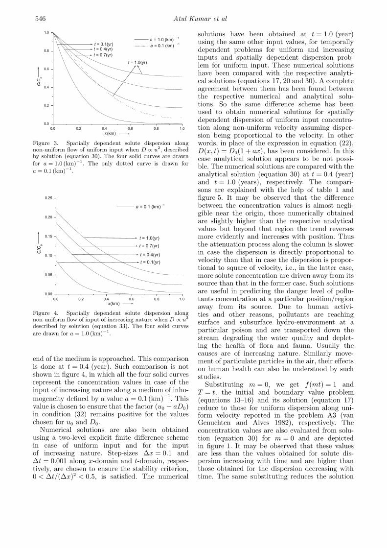
546 Atul Kumar et al

Figure 3. Spatially dependent solute dispersion alongnon-uniform flow of uniform input when D ∝ u2, describedby solution (equation 30). The four solid curves are drawn

for a = 1.0 (km)−1. The only dotted curve is drawn for

a = 0.1 (km)−1.

Figure 4. Spatially dependent solute dispersion alongnon-uniform flow of input of increasing nature when D ∝ u2

described by solution (equation 33). The four solid curves

are drawn for a = 1.0 (km)−1.

end of the medium is approached. This comparisonis done at t = 0.4 (year). Such comparison is notshown in figure 4, in which all the four solid curvesrepresent the concentration values in case of theinput of increasing nature along a medium of inho-mogeneity defined by a value a = 0.1 (km)−1. Thisvalue is chosen to ensure that the factor (u0 − aD0)in condition (32) remains positive for the valueschosen for u0 and D0.

Numerical solutions are also been obtainedusing a two-level explicit finite difference schemein case of uniform input and for the inputof increasing nature. Step-sizes Δx = 0.1 andΔt = 0.001 along x-domain and t-domain, respec-tively, are chosen to ensure the stability criterion,0 < Δt/(Δx)2 < 0.5, is satisfied. The numerical

solutions have been obtained at t = 1.0 (year)using the same other input values, for temporallydependent problems for uniform and increasinginputs and spatially dependent dispersion prob-lem for uniform input. These numerical solutionshave been compared with the respective analyti-cal solutions (equations 17, 20 and 30). A completeagreement between them has been found betweenthe respective numerical and analytical solu-tions. So the same difference scheme has beenused to obtain numerical solutions for spatiallydependent dispersion of uniform input concentra-tion along non-uniform velocity assuming disper-sion being proportional to the velocity. In otherwords, in place of the expression in equation (22),D(x, t) = D0(1 + ax), has been considered. In thiscase analytical solution appears to be not possi-ble. The numerical solutions are compared with theanalytical solution (equation 30) at t = 0.4 (year)and t = 1.0 (years), respectively. The compari-sons are explained with the help of table 1 andfigure 5. It may be observed that the differencebetween the concentration values is almost negli-gible near the origin, those numerically obtainedare slightly higher than the respective analyticalvalues but beyond that region the trend reversesmore evidently and increases with position. Thusthe attenuation process along the column is slowerin case the dispersion is directly proportional tovelocity than that in case the dispersion is propor-tional to square of velocity, i.e., in the latter case,more solute concentration are driven away from itssource than that in the former case. Such solutionsare useful in predicting the danger level of pollu-tants concentration at a particular position/regionaway from its source. Due to human activi-ties and other reasons, pollutants are reachingsurface and subsurface hydro-environment at aparticular poison and are transported down thestream degrading the water quality and deplet-ing the health of flora and fauna. Usually thecauses are of increasing nature. Similarly move-ment of particulate particles in the air, their effectson human health can also be understood by suchstudies.

Substituting m = 0, we get f(mt) = 1 andT = t, the initial and boundary value problem(equations 13–16) and its solution (equation 17)reduce to those for uniform dispersion along uni-form velocity reported in the problem A3 (vanGenuchten and Alves 1982), respectively. Theconcentration values are also evaluated from solu-tion (equation 30) for m = 0 and are depictedin figure 1. It may be observed that these valuesare less than the values obtained for solute dis-persion increasing with time and are higher thanthose obtained for the dispersion decreasing withtime. The same substituting reduces the solution

Analytical solutions of advection–diffusion equation 547

Table 1. Comparison of spatially dependent concentration dispersion along non-uniform flow of uniform input incases (i) D ∝ u2 (analytical solution) and (ii) D ∝ u (numerical solution). In both the cases a = 1.0 (km)−1.

x (km) 0.0 0.1 0.2 0.3 0.4 0.5 0.6 0.7 0.8 0.9 1.0

t = 0.4 (yr)

(i) 1.0 0.794 0.626 0.492 0.388 0.310 0.254 0.216 0.193 0.183 0.182

(ii) 1.0 0.810 0.642 0.498 0.379 0.285 0.213 0.163 0.131 0.115 0.114

t = 1.0 (yr)

(i) 1.0 0.881 0.785 0.707 0.647 0.601 0.568 0.545 0.531 0.525 0.524

(ii) 1.0 0.887 0.786 0.697 0.622 0.559 0.510 0.474 0.450 0.438 0.438

Figure 5. Comparison of spatially dependent concentrationdispersion along non-uniform flow of uniform input in cases(i) D ∝ u2 (analytical solution) and (ii) D ∝ u (numerical

solution). In both the cases, a = 1.0 (km)−1.

(equation 20) to that of the problem A4 (vanGenuchten and Alves 1982). But it may be notedthat although for a = 0, from equations (21 and22) we get u = u0 and D = D0, respectively, hencethe advection–diffusion equation with spatiallydependent coefficients reduces to that with con-stant coefficients but the solution of the latteralong with the same initial and boundary condi-tions cannot be obtained by substituting a = 0 inthe solution (equation 30 or 33) (as the case for theinput may be). It may be verified and understoodfrom the solutions of the two ordinary differentialequations (1 + ax)2y′′ − 3(1 + ax)y′ + 2y = 0 andy′′ − 3y′ + 2y = 0.

It may be observed that while getting the ana-lytical solutions in section 2, the transformationequation (7) has played a key role. A similar trans-formation has been used in section 3 also. In factin the advection–diffusion equation

∂C

∂t=

∂

∂x

(D0f1(x, t)

∂C

∂x− u0f2(x, t)C

),

a substitution like

∂C

∂X= f1(x, t)

∂C

∂x− f2(x, t)C,

is a linear partial differential equation of first orderhence it is equivalent to an auxilliary system ofordinary differential equations, one of which is

dX

−1=

dx

f1(x, t).

Its solution is both the transformations(equations 7 and 23) for f1(x, t) = f(mt) andf1(x, t) = (1 + ax)2, respectively. Though minussign is omitted in transformation (equation 7) itcannot be omitted in equation (23) otherwise theposition x = L in condition (12) will correspondto Z0 = log(−1 − aL) in equation (27). In case thevelocity is linearly interpolated as u = u0(1 − ax)to represent the decrease in it along the mediumcolumn 0 ≤ x ≤ L, one has to proceed with posi-tive sign in (equation 23).

5. Conclusions

Analytical solutions to one-dimensional advection–diffusion equation with variable coefficients alongwith two sets of boundary conditions (in one setinput condition is uniform while in other it is ofincreasing nature while the second condition ineach set is homogeneous of flux type) in an initiallysolute free finite domain have been obtained in twocases:

(i) temporal dependent dispersion along uniformflow through homogeneous medium and

(ii) spatially dependent dispersion along non-uniform flow through inhomogeneous mediumin which solute dispersion is assumed propor-tional to the square of velocity.

The application of a new transformationwhich introduces another space variable, on the

548 Atul Kumar et al

advection–diffusion equation makes it possible touse Laplace transformation technique in gettingthe analytical solutions. Numerical solutions havealso been obtained using a two-level explicit finitedifference scheme. The respective analytical andnumerical solutions have also been compared andvery good agreement between the two has beenfound. The analytical solution of the second prob-lem in case of uniform input has been comparedwith the numerical solution of same problem butassuming dispersion varying with velocity. Suchanalytical solutions may serve as tools in validat-ing numerical solutions in more realistic dispersionproblems facilitating to assess the transport of pol-lutants solute concentration away from its sourcealong a flow through soil medium, through aquifersand through oil reservoirs.

Acknowledgements

The authors express their gratitude to the learnedreviewers for their valuable comments and sugges-tions which improved the present work to a greatextent. This work is part of the research programfor the award of Ph.D. degree to first two authors.Financial supports to both in the form of RajivGandhi National Fellowship and UGC researchfellowship, respectively, from University GrantsCommission, Government of India, are gratefullyacknowledged.

References

Al-Niami A N S and Rushton K R 1977 Analysis of flowagainst dispersion in porous media; J. Hydrol. 33 87–97.

Aral M M and Liao B 1996 Analytical solutions fortwo-dimensional transport equation with time-dependentdispersion coefficients; J. Hydrol. Engg. 1(1) 20–32.

Banks R B and Ali J 1964 Dispersion and adsorption inporous media flow; J. Hydraul. Div. 90 13–31.

Banks R B and Jerasate S R 1962 Dispersion in unsteadyporous media flow; J. Hydraul. Div. 88 1–21.

Bastian W C and Lapidus L 1956 Longitudinal diffusionin ion exchange and chromatographic columns; J. Phys.Chem. 60 816–817.

Bear J 1972 Dynamics of fluids in porous media (New York:Amr. Elsev. Co.).

Bear J and Bachmat Y 1964 The general equations of hydro-dynamic dispersion; J. Geophys. Res. 69 2561–2567.

Brenner H 1962 The diffusion model of longitudinal mixingin beds of finite length. Numerical values; Chem. Engg.Sci. 17 229–243.

Cleary R W and Adrian D D 1973 Analytical solution ofthe convective-dispersive equation for cation adsorptionin soils; Soil Sci. Soc. Am. Proc. 37 197–199.

Crank J 1975 The Mathematics of Diffusion (London:Oxford Univ. Press).

Chrysikopoulos C V and Sim Y 1996 One dimensionalvirus transport in homogeneous porous media withtime-dependent distribution coefficient; J. Hydrol. 185199–219.

Ebach E H and White R 1958 The mixing of fluids flow-ing through packed solids; J. Am. Inst. Chem. Engg. 4161–164.

Gelhar L W, Welty C and Rehfeldt K R 1992 A criticalreview of data on field-scale dispersion in aquifers; WaterResour. Res. 28(7) 1955–1974.

Guvanasen V and Volker R E 1983 Experimental inves-tigations of unconfined aquifer pollution from rechargebasins; Water Resour. Res. 19(3) 707–717.

Harleman D R F and Rumer R R 1963 Longitudinal andlateral dispersion in an isotropic porous medium; J. FluidMech. 385–394.

Hunt B 1978 Dispersion calculations in nonuniform seepage;J. Hydrol. 36 261–277.

Kim Kue–Young, Kim T, Kim Y and Woo Nam-Chil 2007A semi-analytical solution for ground water responses tostream–stage variations and tidal fluctuations in a coastalaquifers; Hydrol. Process. 21 665–674.

Kumar N 1983 Unsteady flow against dispersion in finiteporous media; J. Hydrol. 63 345–358.

Lai S H and Jurinak J J 1971 Numerical approximationof cation exchange in miscible displacement through soilcolumns; Soil Sci. Soc. Am. Proc. 35 894–899.

Leij F J, Toride N and van Genutchen M Th 1993Analytical solutions for non-equilibrium solute trans-port in three-dimensional porous media; J. Hydrol. 151193–228.

Lin S H 1977 Nonlinear adsorption in layered porous mediaflow; J. Hydraul. Div. 103 951–958.

Lindstrom F T and Boersma L 1989 Analytical solutions forconvective–dispersive transport in confined aquifers withdifferent initial and boundary conditions; Water Resour.Res. 25(2) 241–256.

Logan J D and Zlotnik V 1995 The convection–diffusionequation with periodic boundary conditions; Appl. Math.Lett. 8(3) 55–61.

Logan J D 1996 Solute transport in porous media with scale-dependent dispersion and periodic boundary conditions;J. Hydrol. 184 261–276.

Manoranjan V S and Stauffer T B 1996 Exact solutions forcontaminant transport with kinetic Langmuir sorption;Water Resour. Res. 32 749–752.

Marino M A 1974 Distribution of contaminants in porousmedia flow; Water Resour. Res. 10 1013–1018.

Marshal T J, Holmes J W and Rose C W 1996 Soil Physics(Cambridge University Press, 3rd edn.)

Matheron G and deMarsily G 1980 Is transport in porousmedia always diffusive, a counter example; Water Resour.Res. 16 901–917.

Ogata A 1970 Theory of dispersion in granular media; USGeol. Sur. Prof. Paper 411-I 34.

Ogata A and Banks R B 1961 A solution of the differentialequation of longitudinal dispersion in porous media; USGeol. Surv. Prof. Paper 411-A 1–9.

Pang L, Gottz M and Close M 2003 Application of themethod of temporal moment to interpret solute trans-port with sorption and degradation; J. Contam. Hydrol.60 123–134.

Selim H M and Mansell R S 1976 Analytical solution of theequation for transport of reactive solute; Water Resour.Res. 12 528–532.

Severino G and Indelman P 2004 Analytical solutions forreactive transport under an infiltration–redistributioncycle; J. Contam. Hydrol. 70 89–115.

Sirin H 2006 Ground water contaminant transport by nondivergence-free, unsteady, and non-stationary velocityfields; J. Hydrol. 330 564–572.

Shamir U Y and Harleman D R F 1967 Dispersion in layeredporous media; J. Hydraul. Div. 95 237–260.

Analytical solutions of advection–diffusion equation 549

Smedt F De 2006 Analytical solutions for transport of decay-ing solutes in rivers with transient storage; J. Hydrol. 330672–680.

Sposito G, Jury W A and Gupta V K 1986 Fundamentalproblems in the stochastic convection-dispersion modelfor solute transport in aquifers and field soils; WaterResour. Res. 22 77–88.

Tartakovsky D M and Federico V Di 1997 An analyticalsolution for contaminant transport in non uniform flow;Transport in Porous Media 27 85–97.

Tracy Fred T 1995 1-D, 2-D, 3-D analytical solutions ofunsaturated flow in groundwater; J. Hydrol. 170 199–214.

van Genuchten M Th and Alves W J 1982 Analytical solu-tions of the one-dimensional convective-dispersive solute

transport equation; US Dept. Agriculture Tech. Bull. No.1661 151p.

van Kooten J J A 1996 A method to solve the advection-dispersion equation with a kinetic adsorption isotherm;Adv. Water Res. 19 193–206.

Yates S R 1990 An analytical solution for one-dimensionaltransport in heterogeneous porous media; Water Resour.Res. 26 2331–2338.

Yates S R 1992 An analytical solution for one-dimensionaltransport in porous media with an exponential dispersionfunction; Water Resour. Res. 28 2149–2154.

Zoppou C and Knight J H 1997 Analytical solutions foradvection and advection–diffusion equation with spatiallyvariable coefficients; J. Hydraul. Engg. 123 144–148.

MS received 23 September 2008; revised 16 June 2009; accepted 16 June 2009