Comovements in volatility in the euro money market

ISSN 1561081-0

9 7 7 1 5 6 1 0 8 1 0 0 5

WORKING PAPER SER IESNO 703 / DECEMBER 2006

COMOVEMENTS IN VOLATILITY IN THE EURO MONEY MARKET

by Nuno Cassola

and Claudio Morana

In 2006 all ECB publications will feature

a motif taken from the

€5 banknote.

WORK ING PAPER SER IE SNO 703 / DECEMBER 2006

This paper can be downloaded without charge from http://www.ecb.int or from the Social Science Research Network

electronic library at http://ssrn.com/abstract_id=949848

1 The authors are grateful to an anonymous referee of the ECB Working Paper Series and to Steen Ejerskov for constructive comments.2 European Central Bank, Kaiserstrasse 29, 60311 Frankfurt am Main, Germany; e-mail: [email protected]

3 International Centre for Economic Research (ICER, Torino) and University of Piemonte Orientale, Faculy of Economics and Quantitative Methods, Via Perrone 18, 28100, Novara, Italy; e-mail: [email protected]

COMOVEMENTS IN VOLATILITY IN THE

EURO MONEY MARKET 1

by Nuno Cassola 2

and Claudio Morana 3

© European Central Bank, 2006

AddressKaiserstrasse 2960311 Frankfurt am Main, Germany

Postal addressPostfach 16 03 1960066 Frankfurt am Main, Germany

Telephone+49 69 1344 0

Internethttp://www.ecb.int

Fax+49 69 1344 6000

Telex411 144 ecb d

All rights reserved.

Any reproduction, publication andreprint in the form of a differentpublication, whether printed orproduced electronically, in whole or inpart, is permitted only with the explicitwritten authorisation of the ECB or theauthor(s).

The views expressed in this paper do notnecessarily reflect those of the EuropeanCentral Bank.

The statement of purpose for the ECBWorking Paper Series is available fromthe ECB website, http://www.ecb.int.

ISSN 1561-0810 (print)ISSN 1725-2806 (online)

3ECB

Working Paper Series No 703December 2006

CONTENTS

Abstract 4

Non-technical summary 5

1 Introduction 8

2 Econometric methodology 10

3 Data 12

3.1 The variance process 13

4 Empirical results 15

4.1 Descriptive statistics 15

4.2 Structural break tests 15

4.3 Long memory properties 18

4.3.1 Fractional cointegration analysis 19

4.3.2 Permanent-persistent-non persistentdecomposition 20

4.4 The propagation of money marketvolatility shocks 22

4.4.1 Identification of structural shocksand impulse response analysis 23

5 Conclusion 25

6 Appendix A: Estimation of the permanent,persistent, and non persistentcomponents 26

7 Appendix B: Break process estimation,Monte Carlo results 29

References 31

Tables and figures 36

European Central Bank Working Paper Series 51

AbstractThis paper assesses the sources of volatility persistence in Euro

Area money market interest rates and the existence of linkages relat-ing volatility dynamics. The main �ndings of the study are as follows.Firstly, there is evidence of stationary long memory, of similar degree,in all series. Secondly, there is evidence of fractional cointegrationrelationships relating all series, except the overnight rate. Two com-mon long memory factors are found to drive the temporal evolution ofthe volatility processes. The �rst factor shows how persistent volatil-ity shocks are trasmitted along the term structure, while the secondfactor points to excess persistent volatility at the longer end of theyield curve, relative to the shortest end. Finally, impulse responseanalysis and forecast error variance decomposition point to forwardtransmission of shocks only, involving the closest maturities.Keywords: Money market interest rates; liquidity e¤ect; realized

volatility; fractional integration and cointegration, fractional vector er-ror correction model.JEL classi�cation: C32; F30; G10

4ECBWorking Paper Series No 703December 2006

Non-technical summaryRecent work by Prati et al. (2003), Bartolini and Prati (2003a), and

Bartolini et al. (2002) document the close connection between the institu-tional details of the operational frameworks for the implementation of mon-etary policy by central banks and the behavior of overnight interest ratesin the US, the euro area and other G-7 countries. Moreover, Bartolini andPrati (2003b) show that short-term interest rate volatility also re�ects dif-ferences in central banks� commitment to interest rate smoothing at highfrequency. Their evidence is supported by other empirical papers showingthe relevance of institutional details in shaping the behavior of money mar-ket rates and their volatility (see Ayuso et al., 1997; Hartmann et al., 2001).Cassola and Morana (in press) estimate the factors underlying the volatil-ity of the overnight interest rate and its transmission along the euro moneymarket yield curve using hourly data. The estimates show repetitive intra-daily and monthly patterns that can be explained by the microstructure ofthe money market and the institutional features of the Eurosystem�s oper-ational framework for monetary policy implementation. Strong persistenceis detected in all log-volatility processes, and two common long-memory fac-tors are extracted. The �rst factor explains the long-memory dynamics ofthe shortest maturities, while the second factor explains the transmission ofvolatility along the money market yield curve. The present paper comple-ments and extends the study of Cassola and Morana (in press) by consideringa new econometric methodology, a di¤erent log-volatility measure (the real-ized volatility estimator) and an extended and improved data set. Moreover,in the present paper the analysis considers both the short-run and long-runproperties of the data, with cointegration analysis performed by means of thefrequency domain principal components approach of Morana (2004a, 2005)(see also Beltratti and Morana, 2006), and the short-run dynamics estimatedby means of a fractional vector error correction model (F-VECM). Addition-ally, a new approach to permanent-persistent-non persistent decomposition isimplemented. The latter decomposition also allows to shed light on the issueon whether the change in the monetary policy operational framework carriedout by the European Central Bank (ECB) in March 2004 has had any impacton money market volatility. Finally, in the present paper the transmission ofvolatility shocks is investigated by means of impulse response analysis andforecast error variance decomposition. Hence, in addition to the modellingtools employed, the novelty of the paper is also in the empirical analysis, pro-viding evidence on issues so far unexplored for the euro area money market.The empirical approach followed in the paper is broadly consistent with

5ECB


the modelling of the term structure of interest rates proposed by Piazzesi(2001), which generates a money market volatility curve that is U-shaped.Intuitively, such shape can be explained by two di¤erent features. First, liq-uidity noise and other money-market disturbances are shocks to the spreadbetween the overnight interest rate and the central bank target rate (in gen-eral a short-term rate). These shocks a¤ect the term structure of interestrates only at its very short end. Second, the spread between the target rateand the two-year interest rate re�ects the direction of expected future short-term interest rates and, thus, is mainly a¤ected by news about the cyclicalevolution of the economy and the perception, by market participants, of howthe central bank will �react� to such news. These news a¤ect longer-termrates more intensely than they a¤ect intermediate interest rates. This is dueto the fact that markets expect the central bank, when changing short-terminterest rates, to move in a sequence of small steps in one direction, and thesechanges to be somewhat persistent. Thus, the shape of the volatility curveis also related to the expected timing of o¢ cial interest rate decisions andthe �inertia�in policy interest rates. However, in Piazzesi (2001) neither theyields nor the volatility processes for short-term money market interest ratesdisplay long memory.Modelling the term structure of interest rates with fractionally cointe-

grated yields seems to be a largely unexplored territory. One of the fewexceptions is Backus and Zin (1993), which develop a term structure modelwhere yields are driven by the fractionally integrated short-term interest rateprocess. Backus and Zin (1993) argue that the volatility curve implied bythis process matches very closely the average volatility curve observed inU.S. government bond data for the post war period. However, in their modelthe volatility processes are non-stochastic. In contrast, we �nd ample evi-dence that interest rate volatility in the euro money market is stochastic andstrongly persistent. As pointed out by Borio and McCauley (1996), there ispervasive evidence of persistence of volatility in bond markets, i.e. volatilityshocks tend to exercise signi�cant e¤ects for longer than what is expected fora short memory process1, showing a slow hyperbolic pattern of decay, ratherthan a quick exponential one. Three main interpretations have been sug-gested for this phenomenon. The �rst interpretation is that volatility reactsimmediately on the arrival of information, however the arrival of �news�it-self exhibits persistence (Granger, 1980; Andersen and Bollerslev, 1997). Thesecond interpretation is that market participants respond at various speeds toinformation that arrives uniformly over time or to di¤erent volatility dynam-ics (high frequency versus low frequency; Muller et al., 1997), thus generating

1For instance an I(0) process.


persistence. The third one is that persistence re�ects the memory of risk-averse traders. In the paper, the �long memory� property of volatility isaccurately investigated and modelled, also by employing testing approacheswhich are robust to the presence of such a feature.The main �ndings of the study are as follows. Firstly, there is evidence

of long memory in the money market interest rates volatility processes, withtwo common long memory factors driving the temporal evolution of the se-ries analyzed. The identi�ed cointegration space reveals near homogeneousbivariate relationships involving the closest maturities. Moreover, the com-mon long memory factor analysis points to a single factor explaining thetransmission of persistent volatility shocks along the term structure, and toa second factor explaining excess persistent volatility at the longer end ofthe yield curve, relative to the shortest end. Forward propagation of per-sistent volatility shocks is also pointed out by the impulse response analysisand the forecast error variance decomposition, while no evidence of forwardtransmission of liquidity shocks is found.

7ECB


1 Introduction

Recent work by Prati et al. (2003), Bartolini and Prati (2003a), and Bar-tolini et al. (2002) document the close connection between the institutionaldetails of the operational frameworks for the implementation of monetarypolicy by central banks and the behavior of overnight interest rates in theUS, the euro area and other G-7 countries. Moreover, Bartolini and Prati(2003b) show that short-term interest rate volatility also re�ects di¤erencesin central banks�commitment to interest rate smoothing at high frequency.Their evidence is supported by other empirical papers showing the relevanceof institutional details in shaping the behavior of money market rates andtheir volatility (see Ayuso et al., 1997; Hartmann et al., 2001). Cassolaand Morana (in press) estimate the factors underlying the volatility of theovernight interest rate and its transmission along the euro money marketyield curve using hourly data. The estimates show repetitive intra-daily andmonthly patterns that can be explained by the microstructure of the moneymarket and the institutional features of the Eurosystem�s operational frame-work for monetary policy implementation. Strong persistence is detectedin all log-volatility processes, and two common long-memory factors are ex-tracted. The �rst factor explains the long-memory dynamics of the short-est maturities, while the second factor explains the transmission of volatil-ity along the money market yield curve. The present paper complementsand extends the study of Cassola and Morana (in press) by considering anew econometric methodology, a di¤erent log-volatility measure (the real-ized volatility estimator) and an extended and improved data set. Moreover,in the present paper the analysis considers both the short-run and long-runproperties of the data, with cointegration analysis performed by means of thefrequency domain principal components approach of Morana (2004a, 2005)(see also Beltratti and Morana, 2006), and the short-run dynamics estimatedby means of a fractional vector error correction model (F-VECM). Addition-ally, a new approach to permanent-persistent-non persistent decomposition isimplemented. The latter decomposition also allows to shed light on the issueon whether the change in the monetary policy operational framework carriedout by the European Central Bank (ECB) in March 2004 has had any impacton money market volatility. Finally, in the present paper the transmission ofvolatility shocks is investigated by means of impulse response analysis andforecast error variance decomposition. Hence, in addition to the modellingtools employed, the novelty of the paper is also in the empirical analysis, pro-viding evidence on issues so far unexplored for the euro area money market.The empirical approach followed in the paper is broadly consistent with

the modelling of the term structure of interest rates proposed by Piazzesi


(2001), which generates a money market volatility curve that is U-shaped.Intuitively, such shape can be explained by two di¤erent features. First, liq-uidity noise and other money-market disturbances are shocks to the spreadbetween the overnight interest rate and the central bank target rate (in gen-eral a short-term rate). These shocks a¤ect the term structure of interestrates only at its very short end. Second, the spread between the target rateand the two-year interest rate re�ects the direction of expected future short-term interest rates and, thus, is mainly a¤ected by news about the cyclicalevolution of the economy and the perception, by market participants, of howthe central bank will �react� to such news. These news a¤ect longer-termrates more intensely than they a¤ect intermediate interest rates. This is dueto the fact that markets expect the central bank, when changing short-terminterest rates, to move in a sequence of small steps in one direction, and thesechanges to be somewhat persistent. Thus, the shape of the volatility curveis also related to the expected timing of o¢ cial interest rate decisions andthe �inertia�in policy interest rates. However, in Piazzesi (2001) neither theyields nor the volatility processes for short-term money market interest ratesdisplay long memory.Modelling the term structure of interest rates with fractionally cointe-

grated yields seems to be a largely unexplored territory. One of the fewexceptions is Backus and Zin (1993), which develop a term structure modelwhere yields are driven by the fractionally integrated short-term interest rateprocess. Backus and Zin (1993) argue that the volatility curve implied bythis process matches very closely the average volatility curve observed inU.S. government bond data for the post war period. However, in their modelthe volatility processes are non-stochastic. In contrast, we �nd ample evi-dence that interest rate volatility in the euro money market is stochastic andstrongly persistent. As pointed out by Borio and McCauley (1996), there ispervasive evidence of persistence of volatility in bond markets, i.e. volatilityshocks tend to exercise signi�cant e¤ects for longer than what is expected fora short memory process1, showing a slow hyperbolic pattern of decay, ratherthan a quick exponential one. Three main interpretations have been sug-gested for this phenomenon. The �rst interpretation is that volatility reactsimmediately on the arrival of information, however the arrival of �news�it-self exhibits persistence (Granger, 1980; Andersen and Bollerslev, 1997). Thesecond interpretation is that market participants respond at various speeds toinformation that arrives uniformly over time or to di¤erent volatility dynam-ics (high frequency versus low frequency; Muller et al., 1997), thus generatingpersistence. The third one is that persistence re�ects the memory of risk-

1For instance an I(0) process.

9ECB


averse traders. In the paper, the �long memory� property of volatility isaccurately investigated and modelled, also by employing testing approacheswhich are robust to the presence of such a feature.The main �ndings of the study are as follows. Firstly, there is evidence

of long memory in the money market interest rates volatility processes, withtwo common long memory factors driving the temporal evolution of the se-ries analyzed. The identi�ed cointegration space reveals near homogeneousbivariate relationships involving the closest maturities. Moreover, the com-mon long memory factor analysis points to a single factor explaining thetransmission of persistent volatility shocks along the term structure, and toa second factor explaining excess persistent volatility at the longer end ofthe yield curve, relative to the shortest end. Forward propagation of per-sistent volatility shocks is also pointed out by the impulse response analysisand the forecast error variance decomposition, while no evidence of forwardtransmission of liquidity shocks is found.The paper is organized as follows. In Sections 2 and 3 the econometric

methodology and the data employed in the study are presented; in Section 4the empirical results of the study are discussed, while in Section 5 conclusionsare drawn. Finally, methodological details and the results of a Monte Carloexercise aiming to assess the econometric tools proposed in the paper areincluded in the Appendix.

2 Econometric methodology

Consider the following decomposition for the n-variate volatility process yt

yt = �bt +��t + "t;

where bt is a k-variate deterministic common structural break process, �t isa s-variate stationary common long memory process (I(d); 0 < d < 0:5)2, "tis a n-variate residual idiosyncratic I(0) component, � is the n� k commonbreak processes loading matrix, and � is the n � s common long memoryprocesses loading matrix.Following Morana (2006b), estimation of the common factor model is

achieved in two steps.Firstly, a permanent-persistent-non persistent (P-P-NP) decomposition

is carried out for any of the n volatility processes, i.e.

yi;t = b�i;t + �

�i;t + "

�i;t; i = 1; :::; n;

2See Baillie (1996) for an introduction to long memory processes.


where b�i;t, the permanent component, is estimated by b�i;t, computed either by

means of the �exible least squares approach or the adaptive semiparametricapproach described in Appendix A, and ��i;t and "

�i;t, the persistent and non

persistent components, respectively, are estimated by ��i;t and "�i;t, computed

by means of the Fourier transform method of Morana (2006b), also describedin Appendix A.3 Monte Carlo results reported in Morana (2006b) and inAppendix B strongly support the proposed �ltering methodology, pointingto its robustness to the degree of persistence of the actual series, samplesize, presence of observational noise and biased estimation of the fractionaldi¤erencing parameter.Secondly, the common break and long memory processes are estimated

by means of a principal components (PCA) approach, implemented using theestimated permanent and persistent components, as follows

yt = �bt + ��t + "t;

where � = A�1=2

b is the estimated n � k common break processes loading

matrix, �b is the diagonal matrix of the estimated non zero eigenvalues of thereduced rank variance-covariance matrix of the (estimated) break processes�b� (rank k < n), A is the matrix of the associated orthogonal eigenvectors,and bt = �

�1=2b A

0b�t is the k � 1 vector of the standardized (�b = Ik)

principal components or common break processes. Moreover, � = B�1=2

�

is the estimated n � s common break processes loading matrix, �� is thediagonal matrix of the non zero eigenvalues of the reduced rank variance-covariance matrix of the (estimated) long memory components �� (ranks < n), B is the matrix of the associated orthogonal eigenvectors, and �t =��1=2� B

0��t is the s � 1 vector of the estimated standardized (�� = Is)

principal components or common long memory processes. Finally, "t = "�t +

"b;t + "�;t, where "b;t is an n � 1 vector of idiosyncratic components from�bt = �bt+ "b;t and "�;t is an n�1 vector of idiosyncratic components from�t = ��t + "�;t.

4

3Note that the break process b�i;t, the permanent component, can be interpreted as thelong-run forecast for the series yi;t, since lim

s!1Et+syi;t = b�i;t+s; given that for d < 0:5

lims!1

Et+s��i;t = 0, and for b < 0:5 lim

s!1Et+s"

�i;t = 0: On the other hand, the persistent

component, i.e. the long memory component, can be interpreted as the medium-runforecast, since for a su¢ ciently long but �nite forecast horizon lim

s!k<1Et+s(yi;t � b�i;t) =

lims!k<1

Et+s��i;t; since lim

s!k<1Et+s"

�i;t = 0.

4See Morana (2006) also for an extension of the procedure to the non stationary longmemory case (0:5 < d < 1) and to the case of multiple common degrees of persistence.

11ECB


The above principal components approach has been originally proposedby Bierens (2000)5 for the estimation of common deterministic break processes,and extended to the estimation of common long memory processes by Morana(2006). The validity of the proposed estimation procedure has been shownby Bai (2004, 2003) and Bai and Ng (2001). In fact, recent theoretical de-velopments of Bai (2004, 2003) and Bai and Ng (2001) have justi�ed theuse of the PCA estimator also for dependent processes. In particular, Bai(2004) has considered the generalization of PCA to the case in which the se-ries are weakly dependent processes, establishing consistency and asymptoticnormality when both the unobserved factors and idiosyncratic componentsshow limited serial correlation, also allowing for heteroskedasticity in boththe time and cross section dimension in the idiosyncratic components. InBai (2003) consistency and asymptotic normality has been derived for thecase of I(1) unobserved factors and I(0) idiosyncratic components, also in thepresence of heteroskedasticity in both the time and cross section dimensionin the idiosyncratic components. Finally, Bai and Ng (2001) have establishedconsistency also for the case of I(1) idiosyncratic components. As pointedout by Bai and Ng (2001) consistent estimation should also be achieved byPCA in the intermediate case represented by long memory processes. MonteCarlo results supporting the use of the PCA approach also in the case oflong memory processes, and the proposed econometric methodology, havebeen provided in Morana (2006b). It is shown that the performance of theprincipal components approach is indeed not a¤ected by the presence oflong memory, performing well independently of the degree of persistence, thesample size, and the number of factors, being also robust to the presence ofmoderate noise.

3 The data

The data employed in this study are 5-minute observations for the overnightinterest rate, and the one-week, two-week, one-month, three-month, six-month, nine-month and twelve-month EONIA swap rates. Intra-daily obser-vations have been computed as averages of real-time, bid-ask quotes takenfrom REUTERS screens. The raw data were �ltered for typing errors andother outliers using the simple and the dynamic �ltering techniques explainedin Brousseau (2005).6 It is known that these quotes are only indicative. Yet,like Hartmann et al. (2001) it is assumed that there is a close link be-

5This result can not be found in the published version of Bierens (2000) paper.6The authors are grateful to Vincent Brousseau, in the Market Operations Analysis

Division, European Central Bank, for providing the �ltered data.


tween market activity and quotes updating. The sample is from 28/11/2000through 22/04/2005, for a total of 107291 5-minute observations, excludingweekends and holidays. Excluding thin trading days (days in which pricesdid not change) 91392 usable observations are left, i.e. 952 days, with 95�ve-minutes observations each (from 9 a.m. to 5 p.m.).

3.1 The variance process

The daily variance process has been computed by means of the realized vari-ance estimator. Following Andersen et al. (2001) and Barndor¤-Nielsen andShephard (2002), suppose that the logM �1 vector price process, pt, followsa multivariate continuous-time stochastic volatility di¤usion

dpt = �tdt+ tdWt;

where Wt denotes a standard M -dimensional Brownian motion process, andboth the processes for the M �M positive de�nite di¤usion matrix t andthe M-dimensional instantaneous drift �t are strictly stationary and jointlyindependent of the Wt process.Then, conditional on the sample path realization of t and �t, the distri-

bution of the continuously compounded h-period return

rt+h;h = pt+h � pt

is

rt+h;hj��t+� ;t+�

h�=0

� N(hZ0

�t+�d� ;

hZ0

t+�d�):

The integrated di¤usion matrix

hZ0

t+�d�

can be employed as a measure of multivariate volatility.By the theory of quadratic variation, under some weak regularity condi-

tions,

t+h =X

j=1;:::;[h=�]

rt+j��;�r0t+j��;�

p!hZ0

t+�d� ;

13ECB


i.e. the realized variance covariance matrix estimator is a consistent esti-mator, in the frequency of sampling (� ! 0), of the integrated variancecovariance matrix.It is also known thatp

h=��(ii);t;t+h � (ii);t;t+h

�vuuut2 hZ

0

2(ii);t;t+�d�

d�! N (0; 1) :

Since

h=�

3

Xj=1;:::;[h=�]

r4i;t+j��;�p!

hZ0

2(ii);t;t+�d� ;

as �! 0, it follows the feasible limiting distribution�(ii);t;t+h � (ii);t;t+h

�s2

3

Pj=1;:::;[h=�]

r4i;t+j��;�

d�! N (0; 1) ;

showing that the realized variance estimator may be more noisy in highvolatility periods.An additional interesting result concerns the log realized variance, i.e.p

h=��ln (ii);t;t+h � ln(ii);t;t+h

�vuuut2

3

Pj=1;:::;[h=�]

r4(ii);t+j��;� P

j=1;:::;[h=�]

r2(ii);t+j��;�

!2d�! N (0; 1) ;

which, according to Barndor¤-Nielsen and Shephard (2004), provides a moreaccurate asymptotic approximation.On the basis of the above results, daily realized variance ((ii);t) can be

computed from high frequency observations as follows

(ii);t =

HXj=1

r2i;j;t;

where ri;j;tis the return on asset i at the intra-daily observation j for day t:7

7Asymptotic results for the distribution of realized correlations and covariances are alsoavailable, but are not discussed since they are not of interest for the paper.


4 Empirical results

4.1 Descriptive statistics

Descriptive statistics for the daily standard deviation and log standard devi-ation processes are reported in Table 1. As shown in the Table, mean dailyvolatility is highest at the very short end of the yield curve (overnight rateand one-week rate) and at the nine-month level, ranging between 2.6% and3.4%, while the other maturities show a lower but similar mean volatilitylevel (about 1.9%). The volatility of volatility is also highest at the veryshort end of the yield curve (overnight rate, one- and two-week rates), butno clear-cut relationship can be established between the mean level of volatil-ity and the volatility of volatility. According to both the Bera-Jarque andthe Kolmogorov-Smirnov tests, deviations from the normality assumption forthe log standard deviation processes can be detected for all the maturities,suggesting that the rejection of normality may not be determined only by theviolation of the i.i.d hypothesis. The persistence properties of the volatilityseries, in terms of structural breaks and long memory, are assessed below.

4.2 Structural break tests

As a �rst step, in order to avoid biased estimation of the persistence parame-ter8, as well as that (relative) high frequency cyclical e¤ects may a¤ect thedetection of the low frequency deterministic dynamics associated with struc-tural change, the e¤ects of (i) known institutional features of the operationalframework, such as the beginning and end of the maintenance period, thenumber of days between the last allotment and the end of the maintenanceperiod, the �rst and last trading date of the maintenance period, and (ii)of monetary policy related features, such as press conferences following theGoverning Council meeting and interest rate (minimum bid rate) changes,have been removed from the data by regressing the log realized standarddeviation series on impulse dummy variables capturing the above mentionede¤ects.9 Then, structural break and cobreaking tests have been carried outon the purged series. Two methods for candidate break process estimationhave been employed, i.e. the �exible least squares approach of Morana (2006)and the adaptive semiparametric approach of Enders and Lee (2004), as de-scribed in Appendix A. Candidate break processes have been computed by

8See Cassola and Morana (in press).9See Cassola and Morana (in press) for details on the construction of the dummy

variables and their relation to the institutional features of the operational framework ofthe Eurosystem.

15ECB


considering trigonometric expansions up to the eighth order for the adap-tive semiparametric approach. On the basis of the smoothing criterion andthe Monte Carlo results reported in Appendix B, the optimal order of thetrigonometric expansion has been set to four. On the other hand, for the�exible least squares approach one hundred di¤erent values for the penaliza-tion parameter for intercept�s dynamics (i.e., � = 100; 200; :::; 10; 000) havebeen assumed. Then, on the basis of the smoothing criterion and the MonteCarlo results reported in Appendix B the number of selected componentshas been set to twenty six (i.e., � = 100; 200; :::; 2600). Both methods aresuited to extract a slowly varying deterministic non linear trend, which, ac-cording to the decomposition discussed in the methodological section, bearsthe interpretation of long-run forecast o permanent component for the seriesfrom which it is extracted. The estimated candidate break processes andthe processes analyzed are plotted in Figure 1. As is shown in the plot, theestimated break processes are smooth, capturing well the trend dynamics inall the series. The two methods yield similar estimates, although, on thebasis of a smoothness criterion, adaptive estimation may be preferred. Thedegree of commonality among the various processes is also strong for all theseries, apart from the overnight rate, in both cases. In fact, the correlationcoe¢ cient ranges between a minimum of 0.5 and a maximum of 0.9 for allmaturities, apart from the overnight rate. For the latter series the high-est correlation coe¢ cient is about 0.3 for the FLS method, and 0.4 for theadaptive method.To test for spurious break processes, possibly due to neglected long mem-

ory, four complementary tests robust to the presence of long memory havebeen implemented, namely the augmented Engle and Kozicki test (Morana,2002), the Dolado et al. (2004) test, the Teverovsky and Taqqu (1997) test,and the Sibbertsen and Venetis (2004) test. Moreover, in all the cases, tocontrol for small sample e¤ects, the tests have been carried out using criticalvalues obtained by means of the parametric bootstrap.10 The �nal evaluationhas then been carried out by means of a test based on the Bonferroni boundsprinciple. Since four tests have been used, the null of no structural changeat the 5% level can be rejected if in the worst case the null is rejected atthe 1.25% level. The results of the structural break analysis are reported inTable 2, Panels A and B. As is shown in the Table, the structural break testspoint to the rejection of the null of no structural change at the 5% signi�-cance level only for the one-week rate for the case of FLS estimation, and forthe two-week rate only for the case of adaptive estimation. Yet, the evidence

10See Sibbertsen and Venetis (2004) and Poskitt (2005) for a justi�cation of the ap-proach.


is not compelling since, according to the Teverovsky and Taqqu (1997) test,the linear relationship between the log variance and the log level of aggrega-tion of the series becomes weaker (the R2 decreases) in both cases once thebreak process is removed from the series (from 0.98 to 0.95 and from 0.97to 0.92, for the one-week rate and the two-week rate, respectively), as for allthe other series for which the null of no break process has not been rejected.Moreover, the latter result is not spurious and determined by the approachfollowed in the estimation of the candidate break processes, since, as shownin Panel 2, the single common break process pointed by the Bierens (2000)test, is not any longer detected once the test is carried out on the break-freeseries. This latter �nding suggests that, if any, the break process would havebeen adequately modelled by the approaches followed. The results of thecobreaking test may then point to the existence of a single stochastic trenddriving the eight log standard deviation processes, i.e. to seven cointegrationrelationships relating the processes investigated.Hence, the results of the structural change analysis have some interesting

implications for the evaluation of the impact of the changes introduced inMarch 2004 by the European Central Bank (ECB) to its operational frame-work for the implementation of monetary policy.11 These changes were intro-duced with the aim of stabilizing the bidding behavior of banks at the regulartenders of the ECB, and thereby achieving greater stability of money mar-ket conditions. In fact, previous to the changes, expectations of key policyrates changes within the reserve maintenance period created incentives forbanks to either overbid or underbid their true liquidity needs at the Eurosys-tem tenders, depending on whether o¢ cial rates were expected to increaseor decrease, respectively. This in turn created excess volatility in moneymarket conditions (both in liquidity and short-term interest rates), whichoccasionally interfered with the signaling of the monetary policy stance.Since the ECB changed its key policy rates more than one year after the

introduction of the reform (i.e. beyond the sample covered in this study)it is di¢ cult to test the ability of the new framework to cope with expec-tations of interest rate changes. Yet, some useful insights can be gaugedfrom the structural break analysis carried out. The stabilizing impact of theoperational framework should be visible only at the very short end of the

11Firstly, the maturity of the regular main re�nancing operations was reduced from two-weeks to one-week; secondly, the reserve maintenance periods, which started always onthe 24th of each month and ended on the 23rd, were realigned such that they would startafter the ECB�s Governing Council policy decison meeting, which takes place normally onthe �rst Thursday of the month. Moreover, the ECB rates decided at that meeting (thestanding facilities rates and the minimum bid rate of the weekly tenders) would be appliedas of the settlement day of the main re�nancing operation following the policy meeting.

17ECB


money market curve (i.e. below the 1-month maturity). In fact, even with-out expectations of interest rate changes a¤ecting the behavior of marketrates, the reduction in the maturity of the regular re�nancing, the calen-dar adjustment in the reserve maintenance period, and the non-overlappingof liquidity provision across maintenance periods, are changes in the detailsof the operational framework that may matter for the functioning of themoney market. Although some changes in the dynamics of the log-volatilityprocesses seem already visible at the very short end of the money marketcurve, as lower levels in the break processes of the log-volatility of the one-and two-week rates, and the one-month rate may be observed, the estimatedbreak processes are not statistically signi�cant, i.e. none of the maturitiesseems to have been permanently a¤ected by the change in the operationalframework in the period considered. Yet, this �nding does not exclude thatthe change in the operational framework may have had a persistent impacton money market volatility. The declining trend dynamics pointed out bythe estimated candidate break processes, in the light of the outcome of thestructural break tests, actually indicate the latter to be the case. Hence,it is possible to conclude that, while the change in the operational frame-work has not had a permanent impact on money market volatility, i.e. ithas not a¤ected the unconditional expectation of volatility, it has exercisedpersistent e¤ects, i.e. it has a¤ected the conditional expectation of volatility,documented by the declining trend behavior shown by the volatility of theshortest maturities about the time the change took place. It is worthwhilenoting that the subtle, yet important, distinction between permanent andpersistent e¤ects could have not been gauged without the proposed P-P-NPdecomposition.

4.3 Long memory properties

The degree of long memory of the series analyzed has been assessed by meansof semiparametric and parametric estimators of the fractional di¤erencing pa-rameter, implemented, given the outcome of the structural break analysis,using the actual series. In order to achieve robust conclusions, both paramet-ric and semiparametric estimators have been employed. The semiparametricestimators employed belong to two classes, i.e. log periodogram estima-tion (GPH, Geweke and Porter-Hudak, 1983), and local Whittle estimation(Kunsch, 1987; Robinson,1995). Recent extensions to these two classes ofestimators have been considered, aiming to improve the performance of theestimators in the presence of: i) short memory dynamics, (Andrews andGuggenberger (2000) bias reduced log periodogram estimator, Andrews andSun (2004) biased reduced local Whittle estimator, Shimotsu and Phillips


(2002) pooled log periodogram estimator, Moulines and Soulier (1999) broadband log periodogram estimator); ii) observational noise (Sun and Phillips(2003) non linear log periodogram estimator); and iii) non stationarity (Shi-motsu and Phillips (2004) exact local Whittle estimator). The estimator ofRobinson (1998), which has proved to be robust to both bandwidth selectionand the presence of nonstationarity in Monte Carlo experiments, has alsobeen employed. Following Taqqu and Teverovsky (1998), in all the cases the�nal estimates have been obtained as averages over the stable region closestto the zero frequency. On the other hand, parametric estimation of the frac-tional di¤erencing operator has been performed by means of exact maximumlikelihood (Sowell, 1992), modi�ed pro�le likelihood (An and Bloom�eld,1993) and non linear least squares estimation (Beran, 1995). For robustness,the �nal estimate of the fractional di¤erencing parameter for each series hasbeen computed as the median of the estimates obtained by means of the var-ious estimators. The results are reported in Table 3, Panels A-B. As shownin Panel A, the median estimates of the fractional di¤erencing operator arein the range 0.22-0.35, with an average value equal to 0.296 (0.032), and theBonferroni test for the equality of the fractional di¤erencing parameters doesnot allow to reject the null of equality of the fractional di¤erencing parame-ters at the 1% signi�cance level in all cases (Panel B). Hence, in the restof the analysis a common estimate of the fractional di¤erencing parameterequal to the average value obtained from the eight realized log standard de-viation processes, i.e. 0.296 (0.032), has been employed. Finally, no evidenceof observational noise could be detected on the basis of the non linear log-periodogram estimator, providing evidence in favour of the volatility proxyemployed in the study.

4.3.1 Fractional cointegration analysis

The existence of fractional cointegration has been assessed by means of theRobinson and Yajima (2002) fractional cointegrating rank test. In Table 4,Panels A-B, the results of the fractional cointegration analysis are reported.As shown in Panel A, coherent with previous empirical evidence (Cassolaand Morana, in press), the test points to six cointegrating vectors at the1% signi�cance level, with the two implied common long memory factors ex-plaining 100% of total variance at the selected bandwidth (2 ordinates). Thecointegrating vectors have been estimated by means of the frequency domainprincipal components approach proposed by Morana (2004a, 2005; see alsoBeltratti and Morana, 2006), applied to the series in levels. In Table 4, PanelA, the unidenti�ed cointegrating vectors are reported. As shown in the Table,the degree of cointegration is moderate, since the error correction residuals

19ECB


still show some persistence. In fact, the estimated fractional di¤erencing pa-rameters range between 0.15 and 0.24, with an average value equal to 0.191(0.029). Moreover, the Bonferroni test does not allow to reject the null ofequality for the estimated fractional di¤erencing parameters at the 5% level.The identi�cation of the cointegration space has been carried out by relyingon unitary zero frequency square coherence tests and fractional cointegratingrank tests carried out on subsets of variables. Since the information set iscomposed of eight variables and there are six cointegrating vectors, the num-ber of identifying restrictions which needs to be imposed on the cointegratingmatrix for exact identi�cation, in addition to the normalization restrictions,are thirty. As shown in Table 4, Panel B, on the basis of the fractional coin-tegrating rank test, carried out on all the possible subsets of variables, �vebivariate and one trivariate cointegrating relationships could be identi�ed.The fractional cointegrating rank test points to cointegration for four out ofsix cases at the 1% signi�cance level, while for the remaining two cases thesigni�cance level is just over the 10% level. Yet, since in all cases the impliedcommon fractional trend(s) explains over 97% of total variance and the se-lection of the threshold level (0.1) for the Robinson and Yajima (2002) test isarbitrary, it is possible to conclude in favour of the selected structure for thecointegration space. Moreover, support for the identi�ed cointegration spaceis also provided by the zero frequency square coherence analysis. As is shownin Panel B, for all the identi�ed cointegrating vectors the point estimate ofthe square coherence at the zero frequency is very close to the predicted uni-tary value, the null of unity is largely non rejected, and the null of zero squarecoherence is always rejected.12 Finally, from the identi�ed cointegrating vec-tors it is possible to note the forward transmission of volatility shocks fromthe overnight rate to the nine-month rate, moving from all the intermediatematurities considered, i.e. the two-week, one-month, three-month, and thesix-month rate. Forward transmission of volatility shocks is also revealedby the sixth cointegrating vector, from the six and nine-month rates to theone-year rate. Interestingly, in only two cases the null of homogeneity is notrejected by the data, i.e. for the two-week and one-week rates and for thenine-month and sixth-month rates.

4.3.2 Permanent-persistent-non persistent decomposition

Since no signi�cant break processes have been found in the log realized volatil-ity series, the permanent components have been estimated by the sampleunconditional means of the series and the persistent-non persistent decom-

12As shown in Morana (2004b), fractional cointegration implies and is implied by unitarysquared coherence at the zero frequency for the series involved.


position has been carried out by means of the Fourier approach of Morana(2006b), selecting the optimal trimming frequency as the closest one to theorigin at which the decomposition objective is achieved, i.e. a smoothed per-sistent component characterized by a degree of persistence non statisticallydi¤erent from the one determined by the semiparametric analysis (d = 0:296(0:032)), and a non persistent component characterized by a degree of per-sistence non statistically di¤erent from zero.13 The common long memoryfactors have then been computed by applying the principal components ap-proach, detailed in the methodological section, to the estimated persistentcomponents. On the basis of the results of the cointegration analysis, it is ex-pected that two common long memory factors explain the bulk of persistent�uctuations.In Figures 3-4 and Table 5 the results of the persistent-non persistent

decomposition are reported. As shown in the Table, in all the cases the de-composition has been successful in extracting the long memory componentfrom the series, since the estimated fractional di¤erencing operators for thelog volatility series fall in the range 0.28-0.35, and in none of the cases theyare statistically di¤erent, at the 5% level, from the estimated common value,i.e. 0.296. Moreover, coherent with the results of the cointegration analysis,the �rst two principal components account for about 75% of total variance.The estimated factors, with 95% con�dence bounds, are reported in Figure3, while in Figure 4 the estimated persistent components, computed from theestimated factors and factor loadings, are compared with the actual series.14

As shown in the plots, the methodology followed in estimation appears tobe robust to trimming, although the second factor appears to have beenestimated less precisely. Yet, when robustness is assessed on the basis ofthe estimated persistent components, it is very hard to distinguish point es-timates from their 95% signi�cance bounds, since on average the standarderror is only about 10% of the estimated process. As shown by the estimatedfactor loading matrix, the �rst factor a¤ects positively all series, while thesecond factor a¤ects the shorter (up to the two-week horizon) and the longermaturities (from the one-month horizon onwards) with di¤erent signs, re-�ecting an excess persistent volatility component in the longer maturities,relatively to the shorter ones. Overall, the results suggest that the ECB hassuccessfully controlled the shortest end of the yield curve. In fact, the excess

13See Appendix A.14Standard errors have been computed from the corresponding cross-sectional distribu-

tion determined by the sequential trimming followed, with window length determined bythe selected smallest (5) and largest (121) optimal ordinates among the volatility processesanalyzed.

21ECB


volatility of the longer end of the money market curve relative to the shorterend (captured by the second factor) points that the former rates react morepromptly to this factor than the latter do. Coherent with previous �ndingsof Cassola and Morana (in press), it is likely that the excess volatility factorcaptures the �ow of �news�about economic conditions, to which the shorterend of the curve is not �free�to react because of the design of the operationalframework.

4.4 The propagation of money market volatility shocks

The propagation of volatility shocks in the euro area money market has alsobeen assessed by means of impulse response analysis. Coherent with thelong memory properties of the data, impulse responses have been computedfrom a fractionally cointegrated vector error correction (F-VECM) model.Considering the vector of n I(d), 0 < d < 1, fractionally cointegrated longmemory processes (log volatility processes) yt, the F-VECM representation(Engle and Granger, 1987; Dittmann, 2004) of the series can be written as

�(L)(1� L)d (yt �m) =h1� (1� L)d�b

i(1� L)b�zt + "t t = 1; :::; T;

(1)where � (L) = In �

Ppi=1�iL

i is a polynomial matrix in the lag operator,with all the roots outside the unit circle, describing the short-run dynamicsof the system, m is a n� 1 vector of intercepts, d is the estimated commondegree of fractional integration of the actual series, b; 0 � b < d; is theestimated degree of fractional integration of the r-variate estimated vectordisequilibrium processes zt = �

0yt, with the n � r matrix of cointegrating

vectors denoted by �; and the n � r matrix of loadings denoted by �, and"t~IID (0;�). Since, as pointed out in the previous section, the estimationof the cointegration space is semiparametric, the F-VECM model has beenestimated following the Engle and Granger (1987) two-step approach, inthe framework of the thick modelling strategy proposed by Granger andJeon (2004), leading to median estimates and 95% con�dence bounds for theparameters of interest.15

Both information criteria (AIC, BIC) and misspeci�cation tests have beenemployed for the selection of the lag length of the F-VECMmodel. While theinclusion of a single lag is su¢ cient to yield serially uncorrelated residuals,

15In the current framework the �rst step of the Engle and Granger approach requires thedetermination of the order of integration of all series, the estimation of the cointegratingvectors and the determination of their degree of persistence. The second step then concernsthe estimation of the short-run parameters.


according to both the AIC and BIC criteria three lags can be selected.16 Fol-lowing the thick modelling strategy, the parameters of the VECMmodel havethen been estimated by considering VECM(1), VECM(2), and VECM(3)structures, with 1000 Monte Carlo replications for each case. Median esti-mates, as well as 5th and 95th percentiles, have been computed.The estimated loading matrix for the cointegrating vectors is reported in

Table 4, Panels B and C. As is shown in the Table, the results are coherentwith the results of the cointegration analysis, since error correcting behaviorcan be found relatively to all the disequilibria. In particular, the one-monthrate disequilibrium is corrected by the two-week rate; the two-week ratedisequilibrium by the one-week rate; the six-month rate disequilibrium bythe overnight rate, the one-week rate and the own process itself; the three-month rate disequilibrium by the one-month rate; the one-year disequilibriumby the one-month rate and the own process itself; and the nine-month ratedisequilibrium by the three-month rate, the one-year rate and the own processitself. Moreover, none of the volatility series is weakly exogenous relativelyto the long-run parameters at the 5% signi�cance level.

4.4.1 Identi�cation of structural shocks and impulse response analy-sis

Exact identi�cation of the structural shocks has been achieved by means ofthe Choleski decomposition approach. In particular, the following structurehas been assumed for the contemporaneous impact matrix266666666664

i0;ti1w;ti2w;ti1m;ti3m;ti6m;ti9m;ti1y;t

377777777775=

26666664� 0 0 0 0 0� � 0 0 0 0� � � 0 0 0� � � � 0 0� � � � � 0� � � � � �

37777775

266666666664

�i0;t�i1w;t�i2w;t�i1m;t�i3m;t�i6m;t�i9m;t�i1y ;t

377777777775:

The ordering of the variables follows standard theoretical assumptionsconcerning the propagation of shocks along the term structure, with longermaturities showing stronger reactivity to shocks than shorter maturities. Theresults of the forecast error variance decomposition are reported in Table 7,while median impulse response functions, with 95% con�dence bounds, are

16Only for the overnight rate the evidence still points to serially correlated residuals,independently of the inclusion of lagged values of the variables.

23ECB


plotted in Figures 4-11.17 As shown in Table 7, the own shocks explain thebulk of variability (between 71% and 96%) at all horizons for all variables.Moreover, the evidence points to limited forward propagation of volatilityshocks, since for all maturities, apart from the overnight rate and the three-month rate, the own shocks a¤ect non negligibly only the consecutive ma-turities and, at most, within a time horizon of three months. Furthermore,in none of the cases there is evidence of signi�cant backward propagation ofshocks. Finally, according to the forecast error variance decomposition, thebulk of the adjustment is completed within twenty days, with only non signif-icant changes taking place thereafter. The forward propagation of volatilityshocks can also be noted from the impulse response functions. The fol-lowing �ndings are noteworthy. Firstly, an overnight rate shock a¤ects itsown volatility mostly within one day, its e¤ects having faded away alreadywithin �ve days. The overnight rate shock also contemporaneously a¤ectsthe volatility of other maturities within three months, but the e¤ects of theshock are already not signi�cant (at the 5% level) after one day. For matu-rities beyond three months the e¤ects are not signi�cant even contempora-neously. Hence, the �ndings point that liquidity shocks are not transmittedforward along the term structure. On the other hand, the e¤ects of theone-week, two-week and one-month volatility shocks are similar, with shockspropagating forward along the term structure and declining contemporane-ous impact as the maturity increases. While the e¤ects of the one-week rateand two-week rate volatility shocks tend to fade away within ten days, forthe one-month rate the e¤ects tend to be more long lasting. Interestingly,the e¤ects of the two-week rate volatility shock tend to be weaker than forthe other two maturities. Moreover, for all the three maturities signi�cantbackward propagation of shocks can be found, with impact decreasing insigni�cance and magnitude as the shortest maturity is approached. Yet, inthe light of the results of the forecast error variance decomposition, back-ward propagation of shocks does not seem to be an important feature forthe data analyzed. In the light of the common factor analysis, the persis-tent factors may be related to the one-week, two-week and one-month ratevolatility shocks. In particular, the �rst persistent factor may be related tothe one-week and two-week rate shocks, re�ecting the change in the maturityof one of the key ECB policy rates (minimum bid rate of the main re�nancingoperations) occurred in March 2004, and pointing to forward transmissionof persistent shocks, potentially related to ECB monetary policy decisions.

17Median impulse responses have been computed by truncating the in�nite order VARrepresentation for the F-VECM model at 25 lags. The median estimates as well as the95% con�dence intervals have been obtained following the thick modelling strategy.


On the other hand, the second persistent factor may be related to the one-month rate volatility shock, possibly re�ecting the reaction of the market tomacroeconomic news. Finally, also the three-month, six-month, nine-monthand one-year rate volatility shocks, show similar properties, with only for-ward propagation being statistically signi�cant, and declining impact as thematurity increases.Overall, the results con�rm previous �ndings that, di¤erently from per-

sistent shocks, liquidity shocks are not transmitted along the yield curve.Moreover, the absence of backward transmission of shocks from the longerend of the curve suggests that the ECB controls very closely the shortest endof the yield curve.

5 Conclusions

In the paper the persistence of money market interest rates volatility andthe existence of long-run linkages among volatility processes along the termstructure has been analyzed. The main �ndings of the study are as fol-lows. Firstly, the evidence points to a common degree of long memory inthe money market interest rates volatility processes. Secondly, evidence offractional cointegration relationships relating all the series, apart from theovernight rate, and of two common long memory factors, driving the tempo-ral evolution of the volatility processes, has been found. One factor points toforward transmission of persistent volatility shocks along the term structure(�rst factor), and the other factor points to excess persistent volatility af-fecting the longer maturities relative to the shorter (second factor). Forwardpropagation of volatility shocks is also pointed out by the impulse responseanalysis and the forecast error variance decomposition, showing e¤ects fadingaway quickly and mostly a¤ecting closest maturities. Interestingly, while the�rst persistent factor may be related to the ECB policy rate volatility shocks,the second factor may be related to one-month rate volatility shocks. It isconjectured that the second factor in volatility captures the �ow of �news�about economic conditions to which the shorter end of the curve is not �free�to react because of the design of the operational framework.Overall the results suggest that liquidity shocks are not transmitted along

the term structure, and that the ECB has successfully controlled the shortestend of the yield curve. In fact, the excess volatility of the longer end of themoney market curve relative to the shorter end (captured by the secondfactor) suggests that the former rates react more promptly to this factorthan the latter do. Moreover, negligible evidence of backward transmissionof volatility shocks has been found.

25ECB


6 Appendix A: Estimation of the permanent,persistent, and non persistent components

6.1 Estimation of the permanent component

6.1.1 Flexible least squares estimation

Following Morana (2006), estimation of the break processes has been carriedout by means of the FLS estimator. By de�ning the measurement equationas

yt = �t + �yt�1 + "t;

and the associated transition equation as

i;t� i;t�1 ' 0;

where i;t =��t �

�0is the vector parameters in the measurement equa-

tion, the FLS problem can be stated as

min c2i;M ( ) + c

2i;D ( ) ;

where c2M ( ) =XT

t=1"2t is the measurement cost,

c2D ( ) =TXt=2

� t � t�1

�0�� t � t�1

�is the dynamic cost, and � =

��1 00 �2

�is the matrix containing the pe-

nalization terms for parameters dynamics. It is known that lim�!1

j;t;FLS =

j;OLS:The �exible least squares (FLS) estimator of the break process is then

denoted as

bt(�) =�t1� � :

A key issue in FLS estimation is the selection of the value of the penaliza-tion parameters �j. This latter problem has been solved by following a thickmodelling strategy (Granger and Jeon, 2004), i.e. by carrying out estimationover a grid of values, i.e. �1 = f100; 200; :::; 10; 000g, �2 = 106, and thenaveraging over a given number of break process candidates, i.e.

b�H;t =1

H

HXj=1

bj;t;


where H is determined on the basis of a smoothing criterion, i.e. H is suchthat

V [b�H;t]� V [b�H�1;t]V [b�H�1;t]

= s ' 0:

In the empirical implementation s can be optimally set to a small value,i.e. 0.01 or 0.005, determined on the basis of the Monte Carlo results reportedin the Appendix.

6.1.2 Adaptive semiparametric estimation

Following Enders and Lee (2004), the break process can be modelled bymeans of the Gallant (1984) �exible functional form

bt = b0 + b1t+

pXk=1

(bs;k sin(2�kt=T ) + bc;k cos(2�kt=T )) :

Once the number of trigonometric terms is selected, the break processcan then be estimated by running the following OLS regression

yt = bt + "t:

Both a smoothing criterion and the Monte Carlo results reported in theAppendix may be followed to determine the order of the expansion k, whichhas been set to four in the paper. In fact, as far as the Monte Carlo results areconcerned, an expansion of the fourth order is optimal in terms of both theTheil inequality coe¢ cient and the root mean square forecast error criteria,being both values negligible. Moreover, in order to assess the impact ofincreasing the order of the trigonometric expansion on the smoothness of theestimated break process, the break process can been computed for di¤erentorders of the expansion, i.e. k = f1; 2; :::; 8g, and the optimal order of theexpansion can be determined on the basis of a smoothing criterion, i.e. k� issuch that

V [bk�;t]� V [bk��1;t]V [bk��1;t]

= s ' 0.

6.2 Estimation of the persistent and non persistentcomponents

Consider the stationary process fytgT�1t=0 ,

yt = st + nt;

27ECB


where st is the persistent component (I(d), d < 0:5) and nt is the nonpersistent component (I(0)).Then, following Morana (2006b), estimation of the persistent component

st, can be achieved as follows. Firstly, the discrete Fourier transform of yt iscomputed

~yt =1

N

T�1Xk=0

ytei2�k=T :

Then, the portion of the transformed process corresponding to the nonpersistent component is discarded by setting

~y�t =

�~yt 0 � t � H0 t > H

:

Finally, st is estimated by applying the inverse discrete Fourier transformto ~y�t , yielding

st =1

N

T�1Xk=0

~y�t e�i2�k=T :

A two-step procedure for the determination of the trimming frequency2�H=T is proposed. Once the degree of fractional integration (dy) of theprocess yt has been determined, candidate persistent processes are computedby allowing H to vary, i.e. H = f3; 4; :::T � 1g ; computing, in correspon-dence of each value of H, the degree of persistence of the reconstructed per-sistent (ds;H) and non persistent (dn;H) components. The optimal trimmingfrequency is then determined by selecting H in such a way that

ds;H ' dy and dn;H ' 0;

i.e. as the frequency at which the reconstructed persistent component hasa degree of persistence not statistically di¤erent from the one of the ac-tual process and the reconstructed non persistent component has a degreeof persistence not statistically di¤erent from zero.18 In the case more thana frequency satis�ed this latter criterion, the farthest one from the zero fre-quency may be selected in order not to disregard signal potentially belongingto the persistent component. On the other hand, if a smoothed version ofthe unobserved component is sought, or when the non persistent componentmay still be an integrated process I(b), although of lower order than theactual series, i.e. b < d, the optimal trimming frequency may be set equalto the closest one to the zero frequency, still satisfying the above persistence

18See Pollock (2005) for additional details on Fourier series based signal extractionmethods.


requirements. The Monte Carlo results reported in Appendix B provide fullsupport to the proposed methodology.19

7 Appendix B: Break process estimation, MonteCarlo results

The following data generating process has been assumed for the log realizedvolatility process

(1� L)dyt = bt + "t

"t~n:i:d:(0; 1)

b1;t =

�0 1 � t � 5001 501 � t � 1000

b2;t =

8<:0 1 � t � 3001 301 � t � 700�0:5 701 � t � 1000

;

with s = f0:01; 0:007; 0:005; allg; d = f0:2; 0:3; 0:4g; bt = fb1;t; b2;tg; t =1; :::; 1000: The number of replications has been set to 500 for each case.The performance of the estimators has been assessed with reference to the

ability of recovering the unobserved components bt, st, and ft, respectively.The Theil inequality coe¢ cient (IC) and the root mean square forecast error(RMSFE) have been employed in the evaluation

RMSFE =

vuut 1

T

TXt=1

(x�t � xt)2

IC =RMSFEvuut 1

T

TXt=1

x�2t +

vuut 1T

TXt=1

x2t

;

where x�t =1n

nXj=1

xj;t and xj;t is the estimated unobserved component at time

t for replication j, xt = fbt; st; ftg.The results of the Monte Carlo exercise for the break process estimation

approach are reported in Table 8. As is shown in Table 8, the performance

19Note that the proposed methodology could also be employed to compute a signal-noisedecomposition.

29ECB


of both the FLS and the adaptive estimator is not a¤ected by the degree ofpersistence of the series, increasing with the number of trigonometric compo-nents included in the speci�cation (adaptive) and as the smoothing thresholds (FLS) is lowered. While according to the Theil inequality coe¢ cient theadaptive estimator performs well already when a single trigonometric com-ponent is included, a substantial improvement may be noticed by adding anadditional trigonometric component for the single break case and three addi-tional components for the two breaks case. On the other hand, for the FLSestimator averaging over all the candidate break processes does not seem tobe optimal. An optimal threshold can be found by assessing the contributionof the additional candidate to the smoothness of the break process, yieldingan optimal smoothing threshold (s) equal to 0.01. Moreover, both the FLSand adaptive estimators perform best in the case of a single break point thanfor the case of two break points. While both approaches may successfullyrecover an unobserved break process, the FLS approach seems to performslightly better than the adaptive one.


References

[1] Andersen, T.G., T. Bollerslev, F.X. Diebold and P. Labys, 2001, TheDistribution of Realized Exchange Rate Volatility, Journal of the Amer-ican Statistical Association, 96, 42-55.

[2] Andersen, T.G. and T. Bollerslev, 1997, Heterogeneous Information Ar-rivals and Return Volatility Dynamics: Uncovering the Long-Run inHigh Frequency Returns, Journal of Finance, 52, 975-1005.

[3] An, S and P. Bloom�eld, 1993, Cox and Reid�s Modi�cation in Re-gressions Models with Correlated Errors, mimeo, North Carolina StateUniversity, Department of Economics.

[4] Ayuso, J. A. G. Haldane, and F. Restoy, 1997, Volatility TransmissionAlong the Money Market Yield Curve, Review of World Economics, 133,56-75.

[5] Andrews, D.W.K. and P. Guggenberger, 2003, A Bias-Reduced Log Peri-odogram Regression Estimator for the Long Memory Parameter, Econo-metrica, 71, 675-712.

[6] Andrews, D.W.K. and Y. Sun, 2004, Adaptive Local Polynomial WhittleEstimation of Long Range Dependence, Econometrica, 72(2), 569-614.

[7] Backus, D. and S. Zin, 1993, Long-Memory In�ation Uncertainty: Ev-idence from the Term Structure of Interest Rates, Journal of MoneyCredit and Banking, 25 (3), 681-700.

[8] Bai, J., 2004, Estimating Cross-Section Common Stochastic Trends inNonstationary Panel Data, Journal of Econometrics, 122, 137-38.

[9] Bai, J., 2003, Inferential Theory for Factor Models of Large Dimensions,Econometrica, 71(1), 135-171,

[10] Bai, J. and S. Ng, 2001, A Panick Attack on Unit Roots and Cointegra-tion, mimeo, Boston College, NYU.

[11] Baillie, R.T., 1996, Long Memory Processes and Fractional Integrationin Econometrics, Journal of Econometrics, 73, 5-59.

[12] Barndor¤-Nielsen, O. and N. Shephard, 2002, Econometric Analysis ofRealized Volatility and its Use in Estimating Stochastic Volatility Mod-els, Journal of the Royal Statistical Society, Series B, 64, 253-80.

31ECB


[13] Barndor¤-Nielsen, O. and N. Shephard, 2004, How Accurate is the As-ymptotic Approssimation to the Distribution of Realized Variance?, inIdenti�cation and Inference for Econometric Models, ed. by D.F. An-drews, J.L. Powel, and J.H. Stock. Cambridge Univerisity Press, forth-coming

[14] Bartolini L., and A. Prati, 2003 a, The Execution of Monetary Policy:a Tale of Two Central Banks, Economic Policy, 37, 435-467.

[15] Bartolini L., and A. Prati, 2003 b, Cross-Country Di¤erences in Mon-etary Policy Execution and Money Market Rates� Volatility, FederalReserve Bank of New York Sta¤ Report No. 175, October.

[16] Bartolini L., G. Bertola and A. Prati, 2002, Day-to-Day Monetary Policyand the Volatility of the Federal Funds Interest Rate, Journal of MoneyCredit and Banking, 34 (1), 137-159.

[17] Beltratti, A. and C. Morana, 2006, Breaks and Persistence: Macroeco-nomic Causes of Stock Market Volatility, Journal of Econometrics, 131,151-77.

[18] Beran, J., 1995, Maximum Likelihood Estimation of the Di¤erencingParameter for Invertible Short and Long Memory Autoregressive Inte-grated Moving Average Models, Journal of the Royal Statistical Society,57, 659-72.

[19] Bierens, H.J., 2000, Non Parametric Nonlinear Cotrending Analysis,with an Application to Interest and In�ation in the United States, Jour-nal of Businness and Economic Statistics, 18(3), 323-37.

[20] Brousseau, V., 2005, The Spectrum of the Euro-Dollar, in G. Teyssière,A. P. Kirman (Eds.), 2005, Long Memory in Economics, Springer.

[21] Cassola, N. and C. Morana, in press, Volatility of Interest Rates in theEuro Area: Evidence from High Frequency Data, The European Journalof Finance.

[22] Christensen, B.J. and M.O. Nielsen, in press, Asymptotic Normality ofNarrow Band Least Squares in the Stationary Fractional CointegrationModel and Volatility Forecasting, Journal of Econometrics.

[23] Dittmann, I., 2004, Error Correction Models for Fractionally Cointe-grated Time Series, Journal of Time Series Analysis, 25(1), 27-32.


[24] Engle, R.F. and C.W.J. Granger, 1987, Co-integration and Error Correc-tion Representation, Estimation, and Testing, Econometrica, 55, 251-76.

[25] Enders, W. and J. Lee, 2004, Testing for a Unit-Root with a Non LinearFourier Function, mimeo, University of Alabama.

[26] Dolado, J.J., J. Gonzalo and L. Mayoral, 2004, A Simple Test of LongMemory vs. Structural Breaks in the Time Domain, Universidad CarlosIII de Madrid, mimeo.

[27] Gallant, R. 1984, The Fourier Flexible Form, American Journal of Agi-cultural Economics, 66, 204-08.

[28] Geweke, J. and S. Porter-Hudak, 1983, The Estimation and Applicationof Long Memory Time Series, Journal of Time Series Analysis, 4, 221-38.

[29] Granger, C.W. and Y. Jeon, 2004, Thick Modelling, Economic Mod-elling, 21, 323-43.

[30] Granger, C.W.J., 1980, Long-memory Relationships and the Aggrega-tion of Dynamic Models, Journal of Econometrics, 14, 227-238.

[31] Gonzalo, J. and C. Granger, 1995, Estimation of Common Long-MemoryComponents in Cointegrated Systems, Journal of Businness and Eco-nomic Statistics, 13(1), 27-35.

[32] Haldrup, N. and M.O. Nielsen, 2003, Estimation of Fractional Integra-tion in the Presence of Data Noise, Cornell University, mimeo.

[33] Kalaba, R. and L. Tesfatsion, 1989, Time-Varying Linear Regression viaFlexible Least Squares, Computers and Mathematics with Applications,17, 1215-45.

[34] Kunsch, H.R., 1987, Statistical Aspects of Self Similar Processes. InProceedings of the First World Congress of the Bernoulli Society, Y.Prohorov and V.V. Sazanov, eds., 1, 67-74, VNU Science Press, Utrecht.

[35] Hartmann, P., M. Manna and A. Manzanares, The Microstructure ofthe Euro Money Market, Journal of International Money and Finance,20, 895-48.

[36] Morana, C, 2002, Common Persistent Factors in In�ation and ExcessNominal Money Growth and a New Measure of Core In�ation, Studiesin Non Linear Dynamics and Econometrics, 6(3), art.3-5.

33ECB


[37] Morana, C., 2004a, Frequency Domain Principal Components Estima-tion of Fractionally, Cointegrated Processes, Applied Economics Letters,11, 837-42.

[38] Morana, C., 2005, Frequency Domain Principal Components Estima-tion of Fractionally Cointegrated Processes: some New Results and anApplication to Stock Market Volatility, Physica A, 335, 165-175.

[39] Morana<, C., 2004b, Some Frequency Domain Properties of FractionallyCointegrated Processes, Applied Economics Letters, 11, 891-94.

[40] Morana, C., 2006, A Small Scale Macroeconometric Model for Euro-12Area , Economic Modelling, 23 (3), 391-426.

[41] Morana, C. and A. Beltratti, in press, Comovements in InternationalStock Markets, Journal of International Financial Markets, Institutionsand Money.

[42] Morana, C., 2006b, Multivariate Modelling of Long Memory Processeswith Common Components, mimeo, University of Piemonte Orientale.

[43] Moulines, E. and P. Soulier, 1999, Broadband Log-Periodogram Re-gression of Time Series with Long Range Dependence, The Annals ofStatistics, 27(4), 1415-39.

[44] Muller, U.A., Dacorogna, M.M., Davé, R.D., Olsen, R.B., Pictet, O.V.and J.E. von Weizsacker, 1997, Volatilities of Di¤erent Time Resolutions- Analyzing the Dynamics of Market Components, Journal of EmpiricalFinance, 4, 213-39.

[45] Nielsen, M.O. and P.H. Frederiksen, 2004, Finite Sample Comparisonof Parametric, Semiparametric, and Wavelet Estimators of FractionalIntegration, Cornell University, mimeo.

[46] Piazzesi, M., 2001, An Econometric Model of the Yield Curve WithMacroeconomic Jump E¤ects, NBER WP 8246, April.

[47] Pollock, D.S.G., 2005, Econometric Methods of Signal Extraction,mimeo, University of London.

[48] Poskitt, D.S., 2005, Properties of the Sieve Bootstrap for Non-Invertibleand Fractionally Integrated Processes, mimeo, Monash University.


[49] Prati, A., L. Bartolini, G. Bertola, 2003, The Overnight Interbank Mar-ket: Evidence From the G-7 and the Euro Zone, Journal of Banking andFinance, 27, 2045-2083.

[50] Robinson, P.M., 1994, Semiparametric Analysis of Long Memory TimeSeries, Annals of Statistics, 22, 515-39.

[51] Robinson, P.M., 1995, Gaussian Semiparametric Estimation of LongRange Dependence, The Annals of Statistics, 23(5), 1630-61.

[52] Robinson, P.M., 1998, Comment, Journal of Business and EconomicStatistics, 16(3), 276-79.

[53] Robinson, P.M. and Y. Yajima, 2002, Determination of CointegratingRank in Fractional Systems, Journal of Econometrics, 106(2), 217-41.

[54] Shimotsu, K. and P.C.B. Phillips, 2002, Pooled Log Periodogram Re-gression, Journal of Time Series Analysis, 23(1), 57-93.

[55] Shimotsu, K. and P.C.B. Phillips, 2004, Exact Local Whittle Estimationof Fractional Integration, Cowles Foundation Working Paper.

[56] Sibbertsen, P. and I. Venetis, 2004, Distinguishing Between Long RangeDependence and Deterministic Trends, Universitat Dortmund, mimeo.

[57] Sowell, F., 1992, Maximum Likelihood Estimation of Stationary Uni-variate Fractionally Integrated Time Series Models, Journal of Econo-metrics, 53, 165-88.

[58] Sun, Y. and P.C.B. Phillips, 2003, Non Linear Log-Periodogram Regres-sion for Perturbed Fractional Processes, Journal of Econometrics, 115,355-89.

[59] Taqqu, M.S. and V. Teverovsky, 1998, Semi-Parametric Graphical Es-timation Techniques for Long Memory Data, in P.M. Robinson and M.Rosemblatt, eds., Time Series Analysis in Memory of E.J. Hannan,420-32, New York: Springer Verlag.

[60] Teverovsky, V. and M. Taqqu, 1997, Testing for Long Range Dependencein the Presence of Shifting Means or Slowly Declining Trend, Using aVariance Type Estimator, Journal of Time Series Analysis, 18(3), 279-304.

35ECB


Table 1, Panel A: Summary statistics for daily realized standard deviationsi0 i1w i2w i1m i3m i6m i9m i1y

mean 3.296 3.355 1.896 1.879 1.998 1.875 2.554 1.877s.d. 6.367 9.759 7.368 3.511 2.743 2.707 3.012 2.818sk 4.578 6.765 13.066 4.045 3.682 6.101 4.097 8.988ek 29.180 56.511 210.45 21.212 19.260 47.226 26.289 108.73min 0.104 0.010 0.021 0.015 0.048 0.071 0.228 0.235max 64.573 109.72 147.70 32.727 26.128 31.156 34.001 42.513NBJ 0.000 0.000 0.000 0.000 0.000 0.000 0.000 0.000

Table 1, Panel B: Summary statistics for daily realized log standard deviationsi0 i1w i2w i1m i3m i6m i9m i1y

mean 0.175 -0.041 -0.341 -0.345 0.119 0.232 0.545 0.316s.d. 1.352 1.392 1.173 1.348 1.035 0.808 0.831 0.668sk 0.582 0.661 0.572 0.369 0.303 0.535 0.563 1.215ek -0.475 0.629 1.369 -0.197 -0.119 1.222 0.000 2.801min -2.262 -4.630 -3.882 -4.215 -3.044 -2.651 -1.479 -1.450max 4.168 4.698 4.995 3.488 3.263 3.439 3.526 3.750NBJ 0.000 0.000 0.000 0.000 0.000 0.000 0.000 0.000KS 2.849 2.241 1.697 2.074 1.66 1.509 2.491 2.857The table reports summary statistics for daily realized standard deviations

(Panel A) and log realized standard deviations (Panel B). ij ;j = 0; 1w; 2w; 1m; 3m; 6m; 9m; 1y; denotes the overnight rate, the one-weekrate, the two-week rate, the one-month rate, the three-month rate, the sixmonth rate, the nine-month rate and the one-year rate, respectively. NBJ isthe p-value of the Bera-Jarque normality test, while KS is the value of theKolmogorov-Smirnov test (the 99% and 95% critical values are 1.63 and1.36, respectively). The time span analysed is 28/11/2000:22/04/05, for a

total of 952 daily observations.


Table 2, Panel A: Structural break and cobreaking tests, FLS estimation

i0 i1w i2w i1m i3m i6m i9m i1ySBT 0:99 0:01 0:27 0:11 0:05 0.05 0.19 0.24R2

R2bf

0:980:95

0:980:95

0:970:93

0:970:91

0:980:94

0:950:93

0:970:94

0:970:95

r = 1 r = 2 r = 3 r = 4 r = 5 r = 6 r = 7 r = 8CBT 0.019 0.024 0.030 0.064 0.089 0.214 0.627 2.541�

CBTbf 0.014 0.016 0.019 0.020 0.025 0.030 0.031 0.03495% 0.466 0.674 0.860 1.035 1.219 1.411 1.598 1.785

Table 2, Panel B: Structural break and cobreaking tests, adaptive estimation

i0 i1w i2w i1m i3m i6m i9m i1ySBT 0:27 0:04 0:01 0:06 0:11 0.04 0.15 0.15R2

R2bf

0:980:95

0:980:95

0:970:92

0:970:90

0:980:93

0:950:93

0:970:94

0:970:95

r = 1 r = 2 r = 3 r = 4 r = 5 r = 6 r = 7 r = 8CBT 0.019 0.024 0.030 0.064 0.089 0.214 0.627 2.541�

CBTbf 0.011 0.011 0.014 0.015 0.016 0.018 0.021 0.025495% 0.466 0.674 0.860 1.035 1.219 1.411 1.598 1.785

The table reports the results of the (Bonferroni bounds) structural breaktest (SBT ), and the R2 of the log-log variance regression obtained from theTeverovsky and Taqqu (1997) test (actual series and break-free (bf) series).The table also reports the results of the Bierens (2000) cobreaking test (CBT )for the null of up to r cobreaking vectors for the actual and break-free (bf)series. ��denotes rejection at the 5% signi�cance level; �95%�denotes thecritical value for the test.

37ECB


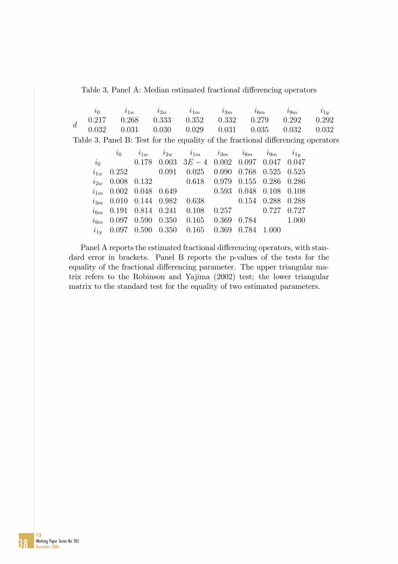
Table 3, Panel A: Median estimated fractional di¤erencing operators

i0 i1w i2w i1m i3m i6m i9m i1y

d0:2170:032

0:2680:031

0:3330:030

0:3520:029

0:3320:031

0:2790:035

0:2920:032

0:2920:032

Table 3, Panel B: Test for the equality of the fractional di¤erencing operators

i0 i1w i2w i1m i3m i6m i9m i1yi0 0:178 0:003 3E � 4 0:002 0:097 0:047 0:047i1w 0:252 0:091 0:025 0:090 0:768 0:525 0:525i2w 0:008 0:132 0:618 0:979 0:155 0:286 0:286i1m 0:002 0:048 0:649 0:593 0:048 0:108 0:108i3m 0:010 0:144 0:982 0:638 0:154 0:288 0:288i6m 0:191 0:814 0:241 0:108 0:257 0:727 0:727i9m 0:097 0:590 0:350 0:165 0:369 0:784 1:000i1y 0:097 0:590 0:350 0:165 0:369 0:784 1:000

Panel A reports the estimated fractional di¤erencing operators, with stan-dard error in brackets. Panel B reports the p-values of the tests for theequality of the fractional di¤erencing parameter. The upper triangular ma-trix refers to the Robinson and Yajima (2002) test; the lower triangularmatrix to the standard test for the equality of two estimated parameters.


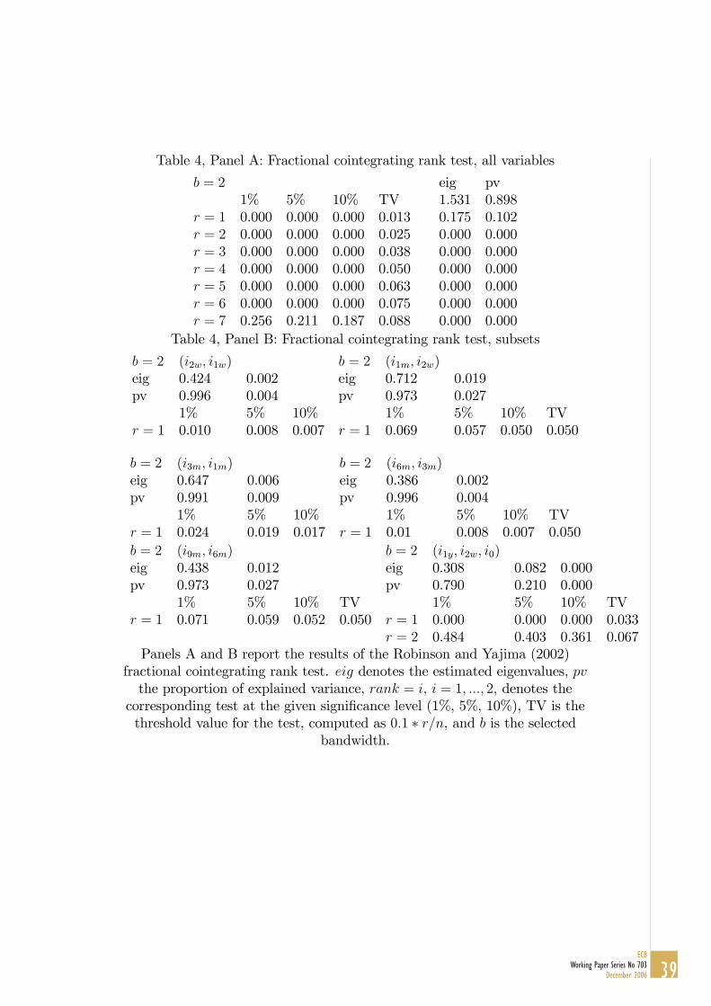
Table 4, Panel A: Fractional cointegrating rank test, all variables

b = 2 eig pv1% 5% 10% TV 1.531 0.898

r = 1 0.000 0.000 0.000 0.013 0.175 0.102r = 2 0.000 0.000 0.000 0.025 0.000 0.000r = 3 0.000 0.000 0.000 0.038 0.000 0.000r = 4 0.000 0.000 0.000 0.050 0.000 0.000r = 5 0.000 0.000 0.000 0.063 0.000 0.000r = 6 0.000 0.000 0.000 0.075 0.000 0.000r = 7 0.256 0.211 0.187 0.088 0.000 0.000

Table 4, Panel B: Fractional cointegrating rank test, subsets

b = 2 (i2w; i1w) b = 2 (i1m; i2w)eig 0.424 0.002 eig 0.712 0.019pv 0.996 0.004 pv 0.973 0.027

1% 5% 10% 1% 5% 10% TVr = 1 0.010 0.008 0.007 r = 1 0.069 0.057 0.050 0.050

b = 2 (i3m; i1m) b = 2 (i6m; i3m)eig 0.647 0.006 eig 0.386 0.002pv 0.991 0.009 pv 0.996 0.004

1% 5% 10% 1% 5% 10% TVr = 1 0.024 0.019 0.017 r = 1 0.01 0.008 0.007 0.050b = 2 (i9m; i6m) b = 2 (i1y; i2w; i0)eig 0.438 0.012 eig 0.308 0.082 0.000pv 0.973 0.027 pv 0.790 0.210 0.000

1% 5% 10% TV 1% 5% 10% TVr = 1 0.071 0.059 0.052 0.050 r = 1 0.000 0.000 0.000 0.033

r = 2 0.484 0.403 0.361 0.067Panels A and B report the results of the Robinson and Yajima (2002)

fractional cointegrating rank test. eig denotes the estimated eigenvalues, pvthe proportion of explained variance, rank = i; i = 1; :::; 2; denotes the

corresponding test at the given signi�cance level (1%, 5%, 10%), TV is thethreshold value for the test, computed as 0:1 � r=n, and b is the selected

bandwidth.

39ECB


Table 5, Panel A: Estimated (unidenti�ed) cointegrating vectors

CV1 CV2 CV3 CV4 CV5 CV6i0 �0:337 �0:113 0:946 0:144 �0:978 0:527i1w �0:240 �1:280 �0:829 0:216 �0:457 �0:214i2w �1:245 1:000 �0:017 �0:319 �0:033 �0:640i1m 1:000 0:354 0:121 �0:178 �1:326 0:014i3m 0:103 0:832 �0:188 1:000 0:492 0:329i6m 0:216 �0:750 1:000 0:106 1:054 �0:498i9m �1:053 �0:375 0:009 �0:205 0:240 1:000i1y 0:821 0:277 �0:257 0:561 1:000 0:538C20 1:000 1:000 1:000 1:000 1:000 1:000T0 0:000 0:000 0:000 0:000 0:000 0:000T1 0:999 0:999 0:999 0:999 0:999 0:999

b0:189(0:029)

0:150(0:029)

0:149(0:029)

0:236(0:029)

0:238(0:029)

0:185(0:029)

Table 5, Panel B: Estimated (identi�ed) cointegrating vectors

CV1 CV2 CV3 CV4 CV5 CV6

i0 0 0 0 0�0:603(0:126)

0

i1w 0�0:992(0:064)

0 0 0 0

i2w�1:459(0:103)

1 0 0�0:695(0:163)

0

i1m 1 0 0�0:496(0:051)

0 0

i3m 0 0�1:359(0:085)

1 0 0

i6m 0 0 1 0 0�0:833(0:083)

i9m 0 0 0 0 0 1i1y 0 0 0 0 1 0C20 0:875 0:984 0:983 0:945 1:000 0:833T0 0:000 0:000 0:000 0:000 0:000 0:000T1 0:974 0:996 0:996 0:988 0:999 0:964


Table 5, Panel C: Loading matrix

i0 i1w i2w i1m

CV10:331

(�0:03 - 0:92)0:258

(�0:26 - 0:74)0:458�

(0:06 - 0:90)0:107

(�0:40 - 0:55)

CV20:079

(�0:47 - 0:59)0:699�

(0:23 - 1:15)�0:032

(�0:50 - 0:36)0:099

(�0:30 - 0:55)

CV3�1:082�

(�2:01 - � 0:52)0:728�

(0:02 - 1:62)0:141

(�0:49 - 0:81)�0:077

(�0:76 - 0:73)

CV40:192

(�0:50 - 1:06)�0:337

(�1:12 - 0:33)�0:101

(�0:74 - 0:43)0:688�

(0:14 - 1:35)

CV50:066

(�0:18 - 0:41)0:017

(�0:31 - 0:31)�0:040

(�0:30 - 0:25)0:295�

(0:01 - 0:64)

CV6�0:442

(�1:32 - 0:30)�0:549

(�1:29 - 0:18)0:131

(�0:62 - 0:76)�0:340

(�1:18 - 0:38)

Table 5, Panel D: Loading matrix

i3m i6m i9m i1y

CV10:125

(�0:20 - 0:52)0:174

(�0:09 - 0:46)0:251

(�0:11 - 0:53)0:043

(�0:23 - 0:28)

CV20:047

(�0:28 - 0:47)�0:020

(�0:28 - 0:23)�0:228

(�0:56 - 0:09)�0:137

(�0:43 - 0:05)

CV30:171

(�0:48 - 0:74)�0:505�

(�1:01 - � 0:15)0:329

(�0:12 - 0:78)0:257

(�0:05 - 0:77)

CV40:191

(�0:48 - 0:64)0:192

(�0:18 - 0:67)0:294

(�0:06 - 0:86)0:159

(�0:14 - 0:56)

CV50:079

(�0:16 - 0:28)�0:101

(�0:27 - 0:08)0:019

(�0:17 - 0:20)�0:167�

(�0:32 - � 0:02)

CV6�0:678�

(�1:34 - � 0:11)0:320

(�0:13 - 0.73)�0:569�

(�1:01 - � 0:16)�0:173�

(�0:60 - 0:21)

Panel A reports the unidenti�ed estimated cointegrating vectors, Panel Breports the identi�ed estimated cointegrating vectors with Christensen andNielsen (in press) asymptotic standard error in parenthesis. C20 is the

estimated simple or multiple square coherence at the zero frequency; T0 andT1 denote the p-values of the zero and unitary squared coherence at thezero frequency test, respectively; b is the estimated fractional di¤erencingparameter for the cointegrating vectors. Panels C and D report the

estimated median loadings, with 95% con�dence intervals in parenthesis.��denotes rejection of the null of zero coe¢ cient at the 5% level.

41ECB


Table 6: Persistent-Non Persistent decomposition

dp dnp m f1 f2

i00:353(0:071)

0:020(0:049)

50:127(0:056)

�0:232(0:066)

i1w0:290(0:061)

0:000(0:022)

420:618(0:059)

�0:292(0:054)

i2w0:281(0:059)

0:084(0:065)

630:646(0:027)

�0:295(0:006)

i1m0:300(0:062)

0:014(0:093)

1210:965(0:008)

0:119(0:007)

i3m0:282(0:057)

0:076(0:090)

730:533(0:062)

0:066(0:031)

i6m0:316(0:067)

0:066(0:065)

640:402(0:016)

0:284(0:034)

i9m0:290(0:062)

0:083(0:062)

830:317(0:036)

0:369(0:032)

i1y0:287(0:061)

0:069(0:091)

900:246(0:028)

0:078(0:026)

pv0:635(0:029)

0:126(0:007)

The table reports the estimated fractional di¤erencing operator for theestimated persistent (p) and non-persistent (np) components, the optimaltrimming ordinate (m), and the estimated factor loading matrix (f1; f2),with the proportion of total variance (pv) explained by each factor.

Standard errors are reported in brackets.


Table 7: Forecast error variance decomposition

1- day �i0 �i1w �i2w �i1m �i3m �i6m �i9m �i1yi0 96:58 1:11 0:78 0:06 0:49 0:17 0:30 0:05i1w 3:05 94:09 0:02 0:28 0:04 0:07 0:05 0:05i2w 3:02 19:51 76:32 0:55 0:05 0:14 0:04 0:06i1m 1:64 13:59 7:21 76:26 0:12 0:33 0:05 0:07i3m 1:22 2:71 3:11 8:69 83:55 0:04 0:14 0:07i6m 0:15 3:42 0:65 4:18 3:18 86:34 1:28 0:26i9m 0:14 1:75 0:23 3:26 1:87 14:01 78:40 0:04i1y 0:25 2:58 0:69 3:55 0:61 6:22 10:73 74:77



20- day �i0 �i1w �i2w �i1m �i3m �i6m �i9m �i1yi0 87:61 3:21 2:76 1:13 1:28 1:18 1:26 0:27i1w 3:21 87:73 4:15 1:90 0:53 0:35 0:78 0:26i2w 3:36 18:76 72:36 2:76 0:45 0:54 0:40 0:29i1m 2:14 13:12 7:02 72:48 2:15 0:74 0:72 0:32i3m 1:78 2:91 3:70 8:74 79:56 0:50 1; 04 0:41i6m 0:49 4:71 1:03 6:33 4:38 79:90 1:73 0:49i9m 0:47 2:29 0:86 4:49 2:25 16:10 72:61 0:32i1y 1:58 3:85 1:06 4:88 0:91 6:25 9:97 70:86

The Table reports the median forecast error variance decomposition.

43ECB


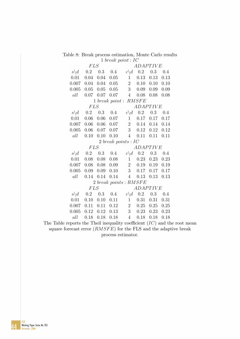
Table 8: Break process estimation, Monte Carlo results1 break point : IC

FLS ADAPTIV Esnd 0:2 0:3 0:40:01 0:04 0:04 0:050:007 0:04 0:04 0:050:005 0:05 0:05 0:05all 0:07 0:07 0:07

cnd 0:2 0:3 0:41 0:13 0:13 0:132 0:10 0:10 0:103 0:09 0:09 0:094 0:08 0:08 0:08

1 break point : RMSFEFLS ADAPTIV E

snd 0:2 0:3 0:40:01 0:06 0:06 0:070:007 0:06 0:06 0:070:005 0:06 0:07 0:07all 0:10 0:10 0:10

cnd 0:2 0:3 0:41 0:17 0:17 0:172 0:14 0:14 0:143 0:12 0:12 0:124 0:11 0:11 0:11

2 break points : ICFLS ADAPTIV E

snd 0:2 0:3 0:40:01 0:08 0:08 0:080:007 0:08 0:08 0:090:005 0:09 0:09 0:10all 0:14 0:14 0:14

cnd 0:2 0:3 0:41 0:23 0:23 0:232 0:19 0:19 0:193 0:17 0:17 0:174 0:13 0:13 0:13

2 break points : RMSFEFLS ADAPTIV E

snd 0:2 0:3 0:40:01 0:10 0:10 0:110:007 0:11 0:11 0:120:005 0:12 0:12 0:13all 0:18 0:18 0:18

cnd 0:2 0:3 0:41 0:31 0:31 0:312 0:25 0:25 0:253 0:23 0:23 0:234 0:18 0:18 0:18

The Table reports the Theil inequality coe¢ cient (IC) and the root meansquare forecast error (RMSFE) for the FLS and the adaptive break

process estimator.


45ECB


Figure 1: Plots 1-6: log realized standard deviations: actual series and FLScandidate break processes (overnight rate (i0), one-week rate (i1w),two-week rate (i2w), one-month rate (i1m), three-month rate (i3m), sixmonth rate (i6m), nine month rate (i9m), twelve-month rate (i1y)). Plots

7-12 FLS (FLS) and adaptive (A) candidate break processes.


Figure 2: Persistent factors with 95% con�dence bounds.

Figure 3: Persistent components (with 95% con�dence bounds) and actualseries.

47ECB


Figure 4: Impulse response functions; unitary overnight rate shock.

Figure 5: Impulse response functions; unitary one-week rate shock.


Figure 6: Impulse response functions; unitary two-week rate shock.

Figure 7: Impulse response functions; unitary one-month rate shock.

49ECB


Figure 8: Impulse response functions; unitary three-month rate shock.

Figure 9: Impulse response functions; unitary six-month rate shock.


Figure 10: Impulse response functions; unitary nine-month rate shock.

Figure 11: Impulse response functions; unitary one-year rate shock.

51ECB


European Central Bank Working Paper Series

For a complete list of Working Papers published by the ECB, please visit the ECB’s website(http://www.ecb.int)

672 “Understanding inflation persistence: a comparison of different models” by H. Dixon and E. Kara,September 2006.

673 “Optimal monetary policy in the generalized Taylor economy” by E. Kara, September 2006.

674 “A quasi maximum likelihood approach for large approximate dynamic factor models” by C. Doz,D. Giannone and L. Reichlin, September 2006.

675 “Expansionary fiscal consolidations in Europe: new evidence” by A. Afonso, September 2006.

676 “The distribution of contract durations across firms: a unified framework for understanding andcomparing dynamic wage and price setting models” by H. Dixon, September 2006.

677 “What drives EU banks’ stock returns? Bank-level evidence using the dynamic dividend-discountmodel” by O. Castrén, T. Fitzpatrick and M. Sydow, September 2006.

678 “The geography of international portfolio flows, international CAPM and the role of monetarypolicy frameworks” by R. A. De Santis, September 2006.

679 “Monetary policy in the media” by H. Berger, M. Ehrmann and M. Fratzscher, September 2006.

680 “Comparing alternative predictors based on large-panel factor models” by A. D’Agostino andD. Giannone, October 2006.

681 “Regional inflation dynamics within and across euro area countries and a comparison with the US”by G. W. Beck, K. Hubrich and M. Marcellino, October 2006.

682 “Is reversion to PPP in euro exchange rates non-linear?” by B. Schnatz, October 2006.

683 “Financial integration of new EU Member States” by L. Cappiello, B. Gérard, A. Kadareja andS. Manganelli, October 2006.

684 “Inflation dynamics and regime shifts” by J. Lendvai, October 2006.

685 “Home bias in global bond and equity markets: the role of real exchange rate volatility”by M. Fidora, M. Fratzscher and C. Thimann, October 2006

686 “Stale information, shocks and volatility” by R. Gropp and A. Kadareja, October 2006.

687 “Credit growth in Central and Eastern Europe: new (over)shooting stars?”by B. Égert, P. Backé and T. Zumer, October 2006.

688 “Determinants of workers’ remittances: evidence from the European Neighbouring Region”by I. Schiopu and N. Siegfried, October 2006.


689 “The effect of financial development on the investment-cash flow relationship: cross-countryevidence from Europe” by B. Becker and J. Sivadasan, October 2006.

690 “Optimal simple monetary policy rules and non-atomistic wage setters in a New-Keynesianframework” by S. Gnocchi, October 2006.

691 “The yield curve as a predictor and emerging economies” by A. Mehl, November 2006.

692 “Bayesian inference in cointegrated VAR models: with applications to the demand foreuro area M3” by A. Warne, November 2006.

693 “Evaluating China’s integration in world trade with a gravity model based benchmark”by M. Bussière and B. Schnatz, November 2006.

694 “Optimal currency shares in international reserves: the impact of the euro and the prospects forthe dollar” by E. Papaioannou, R. Portes and G. Siourounis, November 2006.

695 “Geography or skills: What explains Fed watchers’ forecast accuracy of US monetary policy?”by H. Berger, M. Ehrmann and M. Fratzscher, November 2006.

696 “What is global excess liquidity, and does it matter?” by R. Rüffer and L. Stracca, November 2006.

697 “How wages change: micro evidence from the International Wage Flexibility Project”by W. T. Dickens, L. Götte, E. L. Groshen, S. Holden, J. Messina, M. E. Schweitzer, J. Turunen,and M. E. Ward, November 2006.

698 “Optimal monetary policy rules with labor market frictions” by E. Faia, November 2006.

699 “The behaviour of producer prices: some evidence from the French PPI micro data”by E. Gautier, December 2006.

700 “Forecasting using a large number of predictors: Is Bayesian regression a valid alternative toprincipal components?” by C. De Mol, D. Giannone and L. Reichlin, December 2006.

701 “Is there a single frontier in a single European banking market?” by J. W. B. Bos andH. Schmiedel, December 2006.

702

703 “Comovements in volatility in the euro money market” by N. Cassola and C. Morana,December 2006.

“Comparing financial systems: a structural analysis” by S. Champonnois, December 2006.

ISSN 1561081-0

9 7 7 1 5 6 1 0 8 1 0 0 5

Comovements in volatility in the euro money market

Documents

Transcript of Comovements in volatility in the euro money market