EUROPEAN COMMISSION

The euro and prices: changeover-related inflation and price convergence in the euro area

Jan-Egbert Sturm, Ulrich Fritsche, Michael Graff, Michael Lamla, Sarah Lein, Volker Nitsch, David Liechti and Daniel Triet

Economic Papers 381| June 2009

EUROPEAN ECONOMY

Economic Papers are written by the Staff of the Directorate-General for Economic and Financial Affairs, or by experts working in association with them. The Papers are intended to increase awareness of the technical work being done by staff and to seek comments and suggestions for further analysis. The views expressed are the author’s alone and do not necessarily correspond to those of the European Commission. Comments and enquiries should be addressed to: European Commission Directorate-General for Economic and Financial Affairs Publications B-1049 Brussels Belgium E-mail: Ecfin-Info@ec.europa.eu This paper exists in English only and can be downloaded from the website http://ec.europa.eu/economy_finance/publications A great deal of additional information is available on the Internet. It can be accessed through the Europa server (http://europa.eu ) KC-AI-09-381-EN-N ISSN 1725-3187 ISBN 978-92-79-11192-1 DOI 10.2765/39024 © European Communities, 2009

Content

E c ti summary..................................................................................................1 xe u ve1. Survey and analysis of price developments at the euro changeover..................2 2. The impact of price developments at the euro changeover on different types of households...............................................................................................4 3. Perceived inflation ....................................................................................................................7 4. Cross-border convergence of prices since the euro changeover....................... 10 5. Policy advice ............................................................................................................................. 13 a) Survey and analysis of price developments

at the euro changeover.................................................................................. 17 Summary ............................................................................................................................................... 17 ..................................... 20 a.0) Introduction......................................................................................... a.1) Construction of the HICP..................................................................................................... 20 a.2) A first test to identify unusual movements in the prices at the introduction of the euro.......................................................................................... 22 a.3) Graphical analysis of products that exhibit significant price changes during the cash changeover ............................................................................................... 25 a.4) Graphical analysis of countries that exhibit significant price changes during the cash changeover ............................................................................................... 31 a.5) Yearly and Monthly Price Change Analysis of the Euro Changeover............... 31 a.5.1) Yearly Price Change Analysis.................................................................................32 a.5.2) Monthly Price Change Analysis.............................................................................39 a.6) Out of Pocket Consumption................................................................................................ 45 a.7) Conclusion ................................................................................................................................. 50 References ............................................................................................................................................ 50 Appendix ............................................................................................................................................... 51 b) The impact of price developments at the euro changeover

on different types of households ............................................................... 55 Summary ............................................................................................................................................... 55 b.0) Introduction.............................................................................................................................. 57 b.1) Survey of the literature on group-specific inflation ................................................ 57 b.2) Construction of consumption baskets for different household types ............. 62 b.2.1) Differences in household-specific basket structures ....................................64 b.2.2) Changes in aggregate consumption structure over time ..........................74 b.3) Simulations of price developments ................................................................................ 77 b.4) Econometric evaluation of price effects for different households .................... 98 b.5) Conclusion ...............................................................................................................................120 References ..........................................................................................................................................122 Appendix .............................................................................................................................................124 Box 1 Sensitivity Analysis: 1999 versus 2005 data vintage................................ 124

iii

iv

a) Comparison of weights of the data sets used in the interim report and the newly published 2005 weights ...................................... 124

b) Differences in inflation rates (distribution)............................................ 125 c) Ireland and Greece: a somewhat deeper look ........................................ 126 Econometric methodology ................................................................................................... 133 The clustering approach of Hobijn and Franses (2000) ......................... 133 The PANIC approach of Bai and Ng (2004).................................................. 134 The unit root tests.................................................................................................... 135

c The phenomenon of perceived inflation...............................................137 ) Summary .............................................................................................................................................137 c.0) Introduction............................................................................................................................140 c.1) Survey of the literature on perceived inflation .......................................................140 c.2) Developments of perceived and actual inflation ....................................................143 c.3) Econometric analysis ..........................................................................................................153 c.3.1) Factors driving the perception jumps: national and panel evidence 153 c.3.2) Household-specific inflation rates and inflation perceptions............... 159 c.4) Perceived Inflation and the Media: A Case Study for Germany ........................166 References ..........................................................................................................................................176 Appendix .............................................................................................................................................178 d Cross-border convergence of prices since the euro changeover..179 ) Summary .............................................................................................................................................179 d.0) Introduction............................................................................................................................183 d.1) Survey of the literature on price level convergence under EMU.....................183 d.1.1) Market integration and prices ........................................................................... 183 d.1.2) Price convergence in the European Union.................................................... 186 d.1.3) The euro effect on prices....................................................................................... 187 d.1.4) Summary ..................................................................................................................... 190 d.2) Price data and descriptive results.................................................................................190 d.3) β-and σ-convergence ..........................................................................................................199 d.3.1) All Products ................................................................................................................ 200 d.3.2) Price convergence of tradables and nontradables .................................... 205 d.3.3) Price convergence of 4 product classifications ........................................... 208 d.3.4) Price convergence by category .......................................................................... 211 d.3.5) Price convergence by product ............................................................................ 217 d.4) Determinants of the Speed of Convergence..............................................................219 References ..........................................................................................................................................222 Appendix .............................................................................................................................................224 Product groups.......................................................................................................................... 224 A differences-in-differences approach............................................................................. 230

1

percentage points for year-on-year inflation rates. The third part of the report focuses on inflation perceptions. Survey data indicates that there has been a sizable gap between measured overall inflation (which was low) and inflation perceptions among the broad public (which were relatively large) after the introduction of the euro. Aiming to further explore this puzzling discrepancy (which was not observed before the euro cash changeover), we perform two types of analyses. First, we relate inflation perceptions to observed differences in price developments across different types of households. Second, we examine other potential reasons for the deviation of perceived inflation from actual inflation. While we find that different individual inflation experiences (based on socioeconomic characteristics) help explaining the “jumps” in perception data, a large part still remains unexplained. Searching for other potential determinants, we find that inflation perceptions are mainly

Executive summary This report examines the effects of the introduction of euro notes and coins (“euro cash changeover”) on consumer prices in the euro area. Various aspects of changeover-related price effects are analysed. Issues of (policy) interest range from a quantification of possible price adjustments due to the cash changeover, to potential welfare implications of diverging inflation rates due to differences in household consumption patterns, and the effects of the common currency on the geographical dispersion of prices. The report comprises five parts. We begin by describing price developments at the time of the euro cash changeover. This section aims to identify price anomalies that, potentially, may have been caused by the conversion of prices from national currencies to the euro. Applying various statistical tests, we find that aggregate inflation rates were largely unaffected by the introduction of the euro. For some product groups, however, we observe significant price increases during the period of the euro cash changeover; these categories are mainly in the service sector. We also find considerable differences in product-level price developments across countries. The largest price effects are identified for Finland, where unusual price movements have increased the inflation rate by 0.27 percentage points, while the smallest effects are estimated for Italy with an increase of only 0.004 percentage points. Above that there are countries which do not suffer from any cash changeover related effect at all (e.g., Portugal). In the second part of the report, we examine the effects of price developments at the euro changeover on different types of households. For this purpose, we construct, based on observed differences in consumption patterns, hypothetical consumption baskets for various types of households along various socioeconomic characteristics. In a next step, we confront the observed product-level price movements at the time of the euro cash changeover with the new consumption baskets; this approach allows a quantification of the extent to which changeover-related price changes have affected various household types differently. We find that differences in inflation rates across different types of households are small. Our calculations suggest that deviations of household group-specific inflation rates from the overall HICP rate are in the range of 0.1 to 0.2

2

and taxes). In order to distinguish between normal and exceptional inflation rates, we first compute the difference in the monthly price index over various intervals. These price changes are computed separately for countries and products; the intervals range from 1 month to 6 months. The resulting average inflation rates may then serve as useful benchmark to which we compare price changes at the time of the euro cash changeover. Interestingly, for the majority of products, we observe no extraordinary increase in consumer prices at

driven by lagged perceptions, inflation expectations and actual inflation. Interestingly, a price index of frequently bought items does not outperform an inflation measure based on the HICP in predicting inflation perceptions. Also, the euro cash changeover had a significant effect on those structural relationships, increasing, for instance, the importance of inflation expectations at the cost of the impact of actual inflation. Furthermore, media coverage matters strongly for inflation perceptions. In the fourth part of the report, we examine the effect of the euro on the dispersion of prices across countries. In principle, the introduction of euro notes and coins can be expected to have lowered cross-country price differentials. Prices displayed in a common metric allow easier comparisons, thereby possibly providing better incentives for goods arbitrage. In practice, however, we find no evidence of euro-area specific price convergence after the euro cash changeover. We examine price levels for 224 product groups. In order to control for price developments unrelated to the euro, we compare changes in price differences within EMU to changes in price differentials for other groups of countries, including European Union member countries that have kept their national currency. Applying various econometric techniques, we find that price differentials have generally declined over time across European countries and are relatively smaller for EMU member countries. However, we find no structural change in cross-country price patterns due to the introduction of the euro. Finally, based on our empirical results, we derive some policy implications in section 5 of this executive summary. These policy conclusions may be of particular relevance for countries currently considering the adoption of the euro. 1. Survey and analysis of price developments

at the euro changeover

Consumer price developments in euro area member states We begin our analysis by reviewing consumer price developments in euro area member countries in the period before and after the introduction of euro notes and coins. More specifically, we aim to identify possible changes in consumer prices that can be (directly) related to the euro cash changeover. For this purpose, it is not just sufficient to identify unusual price developments at the time of the introduction of the euro; it is also important to distinguish euro-related price changes from price changes that occurred independently of the cash changeover. To deal with these issues, we apply a battery of statistical tests; we often discuss results only when they turn out to be significant in all of these tests. Also, we discard product groups where price increases were likely driven by other factors (such as energy prices, bad weather or changes in administered prices

3

Identification of price increases due eover at the level of the member state Combining our results from various techniques and different levels of aggregation allows identifying the effect of the euro changeover on inflation. For consistency, we include only price movements that were significantly different in all of the statistical tests that we apply. In addition, price dynamics (trends) have been removed. Therefore, our estimate can be interpreted as a lower bound result. For the euro area, we find that the euro cash changeover has raised inflation by 0.05 percentage points; this comes close to the estimate of 0.09 provided by Eurostat (press release 69/03). If we consider all product groups that exhibit a significant change in prices in at least one of our statistical tests, the price effect of the euro cash changeover increases to about 0.23 percentage point; we consider this result as the upper bound estimate.

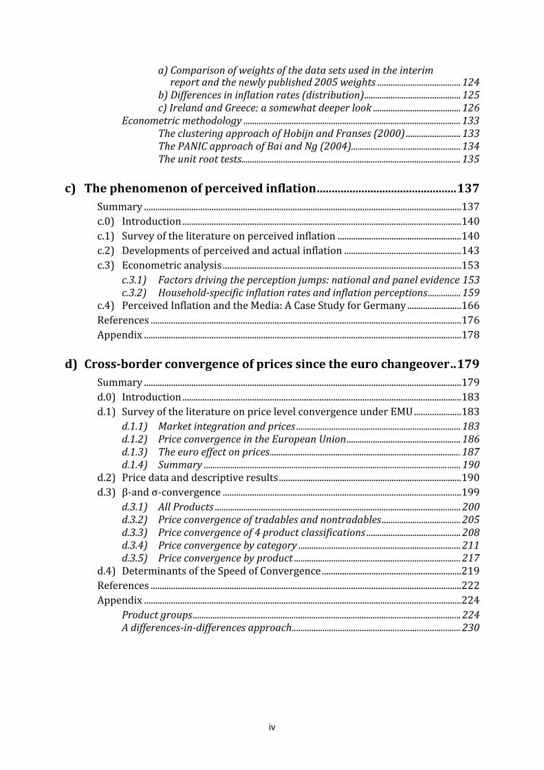
the time of the introduction of the euro. However, significant price increases are found for services; these categories include “catering services”, “cleaning, repair and hire of clothing”, “hairdressing salons and personal grooming establishments”, “restaurants, cafés and the like”, “recreational and sporting services” and “operation of personal transport equipment”. Reviewing the results in more detail, there are also considerable differences across countries. For example, Germany exhibits strong increases in prices for “catering services” and “cleaning, repair and hire of clothing”, which are not observed in, say, Ireland. Overall, prices in the service sector appear to have risen particularly strongly in France and Germany. Comparison of price developments with historical inflation patterns Next, we compare price developments in January 2002 with a counterfactual price measure that is represented by the moving average of price changes. Moving averages are a very flexible tool to capture trends and thereby identify structural breaks; moving averages are computed over various intervals. Interestingly, the largest deviation of euro area inflation from its moving average is in mid-2001, mainly due to a rise in energy prices. From this perspective, the euro cash changeover has not been associated with extraordinary price movements, though practically all EMU member countries, except Ireland, still show unusually strong price increases at the beginning of 2002. These price changes appear to have been more pronounced in EMU member countries than in countries outside EMU. Again, we perform a similar analysis for individual product groups at country level, broadly confirming our earlier results. We also compute a consumption basket of out-of-pocket expenditures that captures prices of frequently bought items. Following the definition provided by the European Central Bank (ECB), this basket includes the categories “food and non-alcoholic beverages”, “alcoholic beverages, tobacco and narcotics”, “non-durable household goods”, “fuels and lubricants for personal transport equipment”, “transport services”, “postal services”, “restaurants and hotels”, and “hairdressing salons and personal grooming establishments”. However, in contrast to other results (most notably Brachinger [2006]), we do not find evidence of unusually strong out-of-pocket inflation in EMU countries during the cash changeover at the beginning of 2002. There appears to be a significant increase in out-of-pocket inflation rates in Germany and France, but rates have been already unusually high during the course of 2001 in these countries.

to the euro chang

4level. Reviewing household consumption baskets, we find some remarkable differences both within countries and across countries. The cross-country differences might be due to differences in consumer preferences, the institutional structure (social security system,

Reviewing estimates for individual countries, we find the largest impact of the euro cash changeover on inflation in Finland, where unusual price movements have increased inflation by about 0.27 percentage points, while the lowest effect is observed in Italy with an increase in the inflation rate by only 0.004 percentage points. Above that there are countries which do not suffer from any cash changeover related effect at all (e.g., Portugal). 2. The impact of price developments at the euro changeover

on different types of households

Survey of the literature on determinants of household consumption Based on our findings for euro-related price changes at the product level, we next analyse the potential welfare effects of these price developments. In particular, we aim to identify the effects of these price changes on households with different socioeconomic characteristics. For this purpose, we define household type-specific consumption baskets and subsequently perform price simulations by combining the newly constructed baskets with actual price data. We begin this section with a brief survey of the relevant literature. Unfortunately, the literature on the determinants of household consumption appears to be underdeveloped. The main contributions date back to the late 1970s and early 1980s when the global increase in inflation that was associated with the dramatic rise in oil prices led to growing concerns about the effects of rising prices on (especially) poor and elderly people. General findings of this literature are that within-group differences in inflation rates are often more pronounced than differences in inflation between groups. Also, there is some evidence that certain groups – most notably, low-income households, old-age households, single-person households – may be, under some circumstances, exposed to somewhat higher inflation, but there is little evidence for “systematic” exposure (since deviations from headline inflation are temporary). Most of the literature refers to results for the United States; studies for European countries are rare. Construction of hypothetical consumption baskets for different household types To construct inflation rates according to household characteristics, we explore data from the “Household Budget Survey” provided by Eurostat. This data set describes the spending structure according to certain household characteristics (employment status of the reference person, the number of active persons, income quintile, type of household, and age of reference person) in 1999. The information on expenditure patterns is merged, at a later stage, with corresponding price data, taken from the price indices of good categories according to COICOP (Classification of individual consumption by purpose)-2 level in the “Harmonized Index of Consumer Prices” (HICP) on a national

5

inflation. Interestingly, an increase in the dispersion of household-specific inflation rates is observable for a number of European countries at the time of the euro cash changeover (i.e., in 2001/2002). However, it is unlikely that this increase is related to the changeover (alone) since similar effects are also observable for some non-EMU

tax system, government-financed benefits), the income distribution, and the general level of economic development of the countries. For Spain, Greece, Portugal, Ireland and the United Kingdom, we also observe sizable within-country differences in consumption baskets. The reasons for these discrepancies may be country-specific, ranging from a more dispersed income and wealth distribution (incl. housing and owner-occupied dwellings) to expenditure-related features of catching-up growth. In Ireland, the United Kingdom and Spain, the differences are particularly pronounced for “housing, electricity, gas and fuels”. When measured as fractions of the overall budget, most of the differences in expenditure structures are (almost by definition) small. A general observation is that poorer households (i.e., households at the lower end of the income distribution, single households and households of unemployed/ retired persons) spend a higher proportion of income in lower COICOP categories, such as food, clothing and housing. In contrast, higher income households and households with more active persons in terms of labour market participation spend higher fractions of their income in higher COICOP categories, such as recreation and culture. We also examine changes in the aggregate consumption structure over the last decade. We find consistent evidence that the portion spent on “food (incl. non-alcoholic beverages)” and “alcoholic beverages and tobacco” is steadily declining in Europe. Similarly, the share spent on “clothing and footwear” has decreased, while the expenditure shares for “housing, electricity, gas and fuels” and “transport” were roughly constant – perhaps partly reflecting the increase in oil prices over the last decade. Balancing the declines, the shares of expenditure spent on “health” are rising in most European countries, although the category’s weight is still low on aggregate level. Also, in a number of countries, the share spent on “hotel and restaurant services” has increased. In sum, there has been a general tendency towards increases in expenditures in service-related COICOP categories which cover goods and services that are often more heavily consumed by households with higher incomes. Simulations of price developments In a next step, we match the consumption baskets with product-level price data to compute household-specific inflation rates. Our calculations suggest that deviations of household group-specific inflation rates from the overall HICP rate are small, somewhere in the range of 0.1 to 0.2 percentage points for yearly inflation rates. Although there is evidence that low-income households, households with no active persons in the labour market, unemployed, single households and pensioners are the population groups most strongly affected by higher inflation, the difference is, on average, very moderate. In fact, if we use a simple statistical procedure to define a significance bound, inflation for these types of households is not significantly different from average inflation. In contrast, higher income households, households with several active persons on the labour market and younger persons appear to be less affected by

6

changeover-related effect might have been at work. • For the third group of countries (Netherlands, Finland, Sweden, UK, and most pronouncedly Ireland), the general tendency that poor and elderly faced a higher inflation holds, but the size of the effect is somewhat stronger. The effect is about twice as high as in the first group of countries (and for Ireland even about three to four times as high). The most obvious explanation for these price

countries (United Kingdom, Sweden). Most notably, comparing our results for household-specific inflation rates with changeover-related price changes identified in the first part of the report, we are not able to confirm that households with higher shares of expenditures in categories which are most probably hit by changeover-related price increases, suffer from generally higher inflation rates. Evaluation of price effects for different households Apart from the small magnitude of deviations from average consumer price developments, it is interesting (and also comforting) to note that there is no evidence of a clustering or a lasting divergence of group-specific inflation rates from average inflation; this result holds irrespective of whether we use the aggregate inflation rate (HICP) or the ‘common component’ as benchmark (with the notable exception of United eKingdom). Hence, ther are no large accumulated price differentials. More specifically, we have accumulated the inflation differentials over different time horizons (1997–2006, 1999–2006, 2002–2006), aiming to explore possible tendencies in inflationary developments that may have been amplified or dampened after the euro cash changeover. It turns out that, for both EU15 and EMU data, the accumulated differentials are small. Over a 10 years horizon, the differences are far less than 10 percentage points; for EMU as a whole even less than 5 percentage points. There have been certain spikes in inflation for types of households which were already identified as having been more prone to higher inflation: poor, single households without children, elderly people. Other types of households faced somewhat lower inflation than indicated by the HICP: single households with children (possibly due to means-tested assistance), households with more than one active person on the labour market, households with 2 adults and children for example. On average, however, the accumulated effects are quite moderate. The picture is slightly different when we explore price developments at country level. bserve th s eMore specifically, we o ree group of countri s: • In the first group (Belgium, Denmark, Germany, Greece, France, Italy, Luxembourg, Austria), the effects are still moderate but somewhat higher than for the EU15 or EMU. Generally, the same tendencies as above hold: poor and elderly people as well as single households were somewhat more prone to inflation in the last decade. In some countries (for instance, Germany), higher income households also faced a slightly higher inflation than the median household in the sample. • The second group (Spain, Portugal) consists of countries were middle- and higher-income groups faced above-average inflation. Here, indeed, a (mild)

7

patterns might be due to the strong cross-household dispersion in the category “Housing, water, electricity, and fuels”. Reviewing the magnitude of group-specific inflation differentials, the ‘common component’ (i.e., the first principal component when combining correlated variables into one single factor) in panels of all household-specific rates in each countries explains the overwhelming bulk of the variance of group-specific inflation rates in almost all countries. Our estimates indicate that the aggregate HICP inflation rate explains about 97–99% of all variance of household-specific inflation rates. In turn, this finding implies that the part of inflation faced by each household and which is not covered by the aggregate inflation rate is indeed very small. Interestingly, countries with real-estate price booms (United Kingdom, Ireland, Spain) seem to deviate in some tests and in the accumulated inflation differentials 3. Perceived inflation

Survey the literature on perceived inflation A core issue in the discussion about possible effects of the euro changeover on prices is the emergence of a sizable gap between official inflation rates as reported by statistical offices and inflation perceptions of consumers. While both series exhibit a strong and stable correlation in all countries before the introduction of the euro, there is a clear mismatch between both series after the introduction of the euro, mainly driven by a dramatic increase in inflation perceptions (often manifested as a jump in levels). The behaviour of perceived inflation during the euro cash changeover has been already well documented. Several explanations to rationalise the developments in inflation perceptions are presented; these explanations include: • the degree of macroeconomic (il)literacy influences the perception, • price movements of frequently bought products (which have been somewhat higher around the cash changeover) gain a higher attention, • there is an asymmetry in the perception of price increases relative to price decreases, • expected price movements influence actual perception, • complicated conversion rates might influence perceptions, • style and tone of media coverage are important channels of price perceptions (agenda setting). For all these explanations, some supportive evidence has been presented in the literature. Empirical studies typically use micro-level price and survey data; other studies present results from experimental designs. Overall, however, the relative importance of the various potential channels is unknown; for some of the proposed mechanisms, evidence turns out to be generally mixed.

8

Explore empirically reasons for deviation of perceived inflation from actual inflation Next, we investigate potential explanations for the observed jump in perceptions. In particular, we test the impact of explanatory variables proposed in the literature on inflation perceptions in Europe. Our baseline regression explains current inflation perceptions with its own lagged value, the level of inflation expectations, HICP inflation and a dummy variable for the euro cash changeover. Following others, we use a six month lag of expectations. Notably, a 12 month lag produces similar results, though people might have quite short-run memories. As inflation perceptions may have been blurred by inflation expectations, we control for this effect (using again data from the balance statistics). To test for the impact of current inflation, we employ both the HICP index as well as an out-of-pocket index (FROOP). The latter index should reflect that perceptions could be more affected by prices of frequently purchased items. The

Analysis of price differentials by household type and perceived inflation We begin our analysis by examining the dynamics in perceived and actual inflation over the period from 1996 to 2007. Perceived inflation is measured by the EU balance statistics; for actual inflation, we refer to the Harmonised Index of Consumer Prices (HICP) taken from Eurostat. We exclude Luxembourg and Malta because of data restrictions. For reasons of comparison, we use Sweden and the United Kingdom as control group. We find that the balance statistics of inflation perceptions tracks the dynamics of HICP inflation remarkably well for the period from 1996 to 2001; in statistical terms, the distance of the mean of both series displays a stationary relationship. However, there is a measurable break in this relationship at the time of the introduction of the euro. In all EMU member countries, perceived inflation dramatically jumps upwards, implying a shift in levels in the distance between inflation perceptions and HICP inflation rates. While a temporary gap between actual and perceived inflation is not unusual (for instance, similar changes in the distance between both inflation measures can be observed for the United Kingdom in 2000), the magnitude and persistence of the increase in perceived inflation are remarkable. Interestingly, while measures of actual and perceived inflation have converged again in Germany, Italy and the Netherlands, there is a persistent gap between both measures in France, Belgium, Greece and Finland. We also explore whether differences in inflation perceptions are associated with differences in household-specific inflation rates. This is an innovative exercise since previous analyses often just focus on inflation dynamics on the aggregate level. Here, we combine two of our data sets – the household-specific inflation rates that we have computed along the categories available from the HBS data of Eurostat and the balance statistics according to certain socioeconomic characteristics. We find indeed evidence that “jumps” in perceptions are partly explained by differences in individual inflation experience. This finding holds for various types of households (divided by income group, income source and age). More generally, the effect has not only the expected sign; the results also show that the jump in perceptions is considerably lower when the household-specific inflation rate is considered. This result is remarkable since, as noted above, the quantitative difference in inflation rates is small.

9

measure of interest is the euro cash changeover dummy which has the value of zero until 2002 and the value of one afterwards. We use monthly observations from 1998 to 2007. In line with the literature, we find that both the lag of perceptions and current inflation expectations have a significantly positive effect on inflation perceptions. In addition, actual inflation turns out to be a robust determinant of perceptions, except for Italy. A more notable result is that the persistence of inflation perceptions has increased dramatically in almost all countries after 2002. Before the introduction of euro notes and coins, the persistence coefficients ranged from about 0.4 to about 0.8. After the euro cash changeover, the degree of persistence ranges from about 0.6 to 0.7 for Ireland and Austria up to estimates of about 1.0 for Germany, Italy and the Netherlands. This result implies that unexplained shocks to perception are highly persistent. Moreover, the explanatory power of HICP inflation decreases dramatically. Furthermore, there is evidence that in some countries the influence of expectations on perceptions has increased. That is, inflation perceptions by consumers appear to be increasingly affected by their own inflation expectations, while putting less weight on official price statistics. However, the results are not robust across countries; for the Netherlands and Austria, we observe that expectations have become less important. Replacing actual HICP inflation rates with a measure of price changes for out-of-pocket expenditures, the marginal effect of this variable is even smaller than before. Hence, inflation measures which take into account frequently bought items do not outperform official price data for aggregate inflation in terms of explanatory power. Exploration of the role of media reports for perceived inflation To explore the relevance of media reporting for the dynamics in inflation perceptions, we perform a case study analysis for Germany on the role of media coverage for public inflation perceptions. We employ two measures of incoming news on inflation. First, we apply simple count variables that capture how often a specific terminology is mentioned in the media. The count measures are obtained by searching through a standard online database of media articles, LexisNexis. In the practical implementation of this approach, we use two popular terms: “Teuro” – which is in fact a combination of expensive/”teuer” and euro in German and became very popular in the media, as well as the expression “euro introduction”. While the latter phrase has no particular implication for inflation perceptions (since it just reminds the public of a particular event related to their currency), the first term clearly presumes that inflation has been and/or will be rising as it has a clear and negative connotation. Second, we use data from Medientenor, a research institute that analyses media articles (TV and press) and provides careful codification. From this source, we have obtained media data covering statements dealing with inflation which are at least five lines long (in case of printed media) and last at least five seconds (for television broadcasts). The coding is based on the standards of the media content analysis. We are provided with the overall number of reports in that given period and the amount of reports dealing with rising or falling inflation.

10on trade. Overall, the results from this literature are fairly conclusive. There is generally little evidence that price levels among EMU member countries have converged due to the

Interestingly, we find that media reporting intensity and tone have indeed a significant impact on inflation perceptions. There is clear empirical evidence that the “teuro” debate in the media has driven inflation perceptions in Germany. In addition, news on prices materialise in inflation perceptions in an asymmetric manner, with news on rising inflation having on average much larger effects. Considering the economic magnitude of various determinants of inflation perceptions, media news outperform actual inflation numbers, especially in the second half of the sample. Examining the impact of media news according to various socioeconomic characteristics provides no conclusive evidence. In sum, we find empirical support for explanations of the gap between actual and perceived inflation, based on expected price movements, media coverage and the asymmetry of the reaction to price increases. In contrast, there is no evidence that macroeconomic illiteracy or the impact of frequently bought products have affected inflation perceptions. 4. Cross-border convergence of prices since the euro changeover

Survey of the literature on price level convergence under EMU The dispersion of prices across countries is often used as a measure of market integration: large differences in price levels indicate the existence of barriers to trade, while low price differentials suggest functioning goods market arbitrage. As a result, given the strong interest in the extent of market integration, a number of studies have already empirically analysed the effect of the euro on prices. Broadly, there are three groups of recent works that deal with this issue. A first set of papers is mainly concerned with the ‘border effect’, i.e., the finding that prices vary more significantly across borders than for pairs of cities located within the same country, after holding constant for other factors. Since a potential explanation for this discrepancy may be the use of separate national currencies in different countries, these papers aim to identify the effect of sharing a single currency (i.e., membership in a currency union) on price differentials; the formation of EMU provides an almost perfect ‘natural experiment’ to analyse this issue. A second set of papers is mainly concerned with the extent of market integration in the European Union. The formation of the ‘Single European Market’ in 1993 aims to remove, among other things, any remaining barriers to the movement of goods. Analysing the evolution of price dispersion within the European Union then allows tracking the success of these policies; lower barriers to trade should be associated with smaller price differentials. With the introduction of the euro, simply another dimension is added in these studies. Finally, there are a growing number of papers that focus directly on the euro’s effect on prices. Apart from the fact that this is an interesting research question in itself, these papers mainly contribute to the larger literature on the effects of the euro on economic activity. Most notably, this work complements extensive research on the euro’s effects

11

should observe a structural break in this trend (i.e., an acceleration). Summarising our empirical results, we find consistent evidence for β-convergence in price levels. When comparing the magnitude of the estimated coefficients for various country groups and time periods, the speed of convergence seems to have slightly decreased for EMU member countries after the euro cash changeover, while it has increased for non-EU countries in our sample in recent years. An intuitive explanation

introduction of a common currency. For one thing, price dispersion among EMU member countries was already disproportionately low at the time when the euro was adopted. More importantly, most changes in dispersion after the introduction of the euro are also observable for non-EMU countries. The single study that finds significant euro effects on prices is Allington, Kattuman and Waldmann (2005). Since we use essentially the same data set, we discuss their results in more detail, showing that their estimation results are not robust. Analysis of price level convergence per product group Any analysis of price level convergence faces the problem of usable data. In principle, the price data should display the following features: (i) the product definitions should be identical across locations (otherwise prices are hardly comparable); (ii) the price data should be in levels rather than indexes (otherwise only second moments can be analysed); and (iii) the data set should comprise both national and international locations (otherwise it is impossible to identify a ‘border effect’). These types of data are rare. We use a data set provided by Eurostat. This data set reports price levels for 224 product groups; the data are provided as price indices on country level. Since there are also a number of other data problems (e.g., problems related to the compilation of the price information), our price data is far from perfect. To minimize potential biases, we often analyse sub-sets of the available data. We begin our empirical analysis by comparing the levels of product prices across countries. In particular, we aim to analyse whether the cash changeover to the euro has been accompanied by an increase in market integration and, thus, a decline in the dispersion of price levels among member countries of EMU. To test for price convergence, we essentially borrow two econometric techniques from the literature on economic growth. The concept of β-convergence implies a catching-up process in which countries with initially lower price levels experience faster subsequent increases in prices (i.e., higher inflation) than countries with a previously relatively high level of prices. This implication is usually tested empirically by regressing changes in prices on initial price levels. A negative correlation would then indicate that prices grow on age slo taver wer when hey are initially high and vice versa. The second concept, σ-convergence, analyses the evolution of price dispersion over time; convergence implies a decrease in the dispersion of price levels across countries. In our empirical implementation, we test for this type of convergence by regressing the coefficient of variation, which is a standard measure of price dispersion, on a simple time trend variable. If there is convergence, the coefficient on this variable should be significantly negative. If the euro cash changeover has affected price dispersion, we

12

for this finding is that price levels in EMU countries were already very close to each other. In contrast, price levels in non-EU countries (Iceland, Norway and Switzerland) were initially well above the EMU average and, therefore, can be expected to have fallen over time. For σ-convergence, our results indicate a significant decline in price dispersion over the period from 1995 to 2005. Price dispersion has fallen for both EMU member countries and non-EMU members. Interestingly, the pace of reduction in price dispersion remains roughly unchanged for EMU countries after the introduction of the euro, while it has slowed considerably in non-EMU countries. These relatively more favourable developments for countries that have adopted the euro might be interpreted as positive effects of the common currency. However, our estimates of the decline in price dispersion are typically much larger in magnitude for non-EMU countries—an effect that may have become smaller over time. Discussion of price convergence of non-tradable goods We next separate goods and services along various dimensions. For instance, we distinguish between tradable and non-tradable goods and services, expecting that the euro’s price effects have been relatively larger for tradable products. In practice, we find that price convergence has accelerated after the introduction of the euro, but particularly strongly for price of non-tradable goods and services. We also examine price convergence for individual products and various product groups. For product groups, we find consistent evidence of price convergence between EMU member countries for “recreation and culture”. On product level, we find evidence for β- and σ-convergence only for two product categories: “lamb, mutton and goat” and “jewellery, clocks and watches”. Examination of factors that drive the speed of convergence Finally, we explore potential determinants of price differences across countries. More specifically, we regress bilateral price differences, as measured by the mean squared error, on various country pair-specific characteristics and a comprehensive set of country-specific fixed effects. Our structural control variables include the geographic distance (as a proxy for trade frictions), common membership in EMU, differences in labour costs and differences in the share of tradables in the consumption basket. Our results are not particularly encouraging. Similar to most previous studies, we find that distance has a negative effect on price differences (that is, the larger the distance, the higher the bilateral price differential). Also, institutional integration matters; when both countries are (or later become) member of either the EMU or EU in our sample, their price differentials are significantly lower. Most notably, however, EMU membership has no separate effect on price differentials after 2002, implying that price differences within EMU have been already low before the introduction of the euro. Somewhat disappointingly, neither differences in unit labour cost nor differences in the weight of tradables in the consumption basket have a significant effect on the speed of price dispersion.

13

old currency. Second, given that we observe price increases for some goods and services during the euro cash changeover, it appears advisable for consumers to carefully track prices and, if necessary, to adjust their consumption patterns. Increasing the public’s awareness and sensitivity to the likelihood of price-setting behaviour by firms that aims to test upper price limits should raise the price elasticity of demand. Consequently, demand would be shifted to firms that basically comply with the rule that prices after the cash changeover are old prices (in national currency) multiplied by the conversion rate. An information

5. Policy advice This section aims to draw possible policy conclusions from our findings concerning the effects of the euro cash changeover on prices. The lessons may be of particular relevance for countries currently considering the adoption of the euro. More generally, experiences from EMU are potentially of interest for countries aiming to enter or establish other multinational currency unions, thereby facing similar types of problems of ensuring a smooth transition from the national currency to the new common n ort. currency. I the following, we proceed along the lines of the structure of this repWe begin by drawing possible policy recommendations from our analysis of price developments around the time of the euro cash changeover. As reported in part 1 of our report, we find that the introduction of euro notes and coins had no separately identifiable, significant impact on aggregate inflation rates. Consumer price inflation has been, at worst, marginally higher in January 2002 than in previous or subsequent months. According to our computations, the overall price effect ranges from 0.05 to about 0.23 percentage points for inflation in the euro area. Yet, at the disaggregated level, we find that prices of some product groups, mainly in the service sector, exhibit significant price increases during the introduction of euro notes and coins; this pattern is not observed in countries outside the euro area. Also, we find that the euro effect on prices was quite heterogeneous across the EMU member countries. Substantial effects in the above mentioned sectors and types of businesses can be traced in Finland, France and Germany, with largest effects observed for Finland. However, even in Finland, where unusual price movements increased the inflation rate by about 0.26 percentage points, the overall effect is still relatively small. As a result, we hypothesize that the public outrage about price increases after the introduction of the euro has to be attributed to increases in prices of specific goods and services rather than to a general increase in inflation. Based on this assessment, there are two possible policy recommendations: First, regarding the supply side of goods and services, a mandatory dual display of prices may be helpful. The dual display of prices allows consumers to better track and compare the evolution of prices. Interestingly, countries that have used a dual pricing system (such as Austria) appear to have experienced relatively smaller price effects of the introduction of the euro. In practical implementation, the required time span for this system seems to be debatable. Short periods of showing prices in different currencies imply the risk of a simple delay in price adjustments (that is, prices are increased immediately after the period of dual price display has ended). In contrast, long periods (that is, periods exceeding more than one year) imply the risk of continuous public usage of prices in the

14

2002 do not justify specific support measures. Examining the increase in inflation perceptions at the time of the cash changeover, we find, among other results, that changes in prices for out-of-pocket expenses do not outperform changes in the aggregate price index in explaining the increase in perceptions. As a result, our findings question the recent concentration on frequently bought items as the major argument for the jump in perceptions. In contrast, peoples’ perceptions appear to be partly driven by household-specific inflation rates, as defined

campaign might be particularly useful in this respect. The campaign could be supplemented by close institutional monitoring of prices where changeover-related price hikes are most likely to be expected. The monitoring could reveal unusual price movements, subsequently providing information for the general public. In contrast, direct price controls or price stops are not advisable; these tools interfere with market mechanisms and may lead to price jumps directly after the control is lifted. Similarly, businesses should be educated that past experience clearly shows that price increases at the time of the changeover will not go undetected by the general public. Such an information campaign could be supplemented by measures to prevent abuses, es. like fair pricing rules that can be sanctioned by public listings of offenders and/or finIn addition, it should be noted that prices for goods and services (as well as rates and fees) are often adjusted on a yearly basis. In particular, various studies show that a disproportionately large number of price adjustments take place at the beginning of a year. Since it is difficult for consumers to distinguish between “regular” and changeover-related price changes, it would be advisable to perform the changeover on a date which does not correspond to the time when yearly price adjustments are usually performed. From this perspective, the end of the calendar year does not appear to be the preferred time for a changeover. Choosing another date for the changeover makes it considerably easier to identify product groups that try to exploit the changeover for price adjustments. Still, there are other considerations (such as accounting issues) that may justify the decision to perform the changeover on 1 January. For household-specific inflation rates, we find that price changes affect households along various socio-economic characteristics differently, though within-group differences in inflation are often more pronounced than differences in inflation between groups. Although we find that some types of households – low income households, old-age households, and single person households – are exposed to somewhat higher inflation, there is little evidence that higher exposure of specific groups to consumer price inflation is persistent. Consequently, the general fact that we are able to identify household-specific inflation rates does not imply any particular prediction about how .various groups of the population have been affected by the euro cash changeover As a result, targeting of particular socio-economic subgroups appears to be not warranted. Only if there is clear evidence that a specific group of the population is particularly hard hit by changeover-related inflation, compensatory measures could be contemplated. Policies supporting socio-economic groups that, due to inherent consumption patterns, are faring considerably worse than others, should always be on the agenda of socially responsible governments. Yet, experiences from the changeover in

15

in section 2 of the report, indicating that a closer monitoring of household-specific inflation might be useful. In addition, we find that communication towards the public is of major importance. We present convincing evidence that excessive media reporting on rising prices triggered a strong and largely unjustified increase in inflation perceptions. Given the subsequent persistence of high inflation perceptions in some EMU member countries, a proper communications strategy that highlights potential reasons for the possible discrepancy between officially-reported and personally-observed inflation rates appears recommendable. Communication by Eurostat or DG ECFIN could be seen as a complementary instrument to the information provided by the ECB, reinforcing the importance, accuracy and reliability of official inflation figures. Concerning price dispersion, there is little evidence of a changeover-related increase in price convergence. Still, price convergence has continued after the introduction of the euro. In this respect, there seems to be scope for further deepening of the internal market and structural reforms aimed at increasing competition and market openness.

16

17

a) Survey and analysis of price developments at the euro changeover

Summary Part a) examines price changes during the cash changeover and tests to which extent specific price movements can be attributed to the introduction of the euro. In the con-duct of the analysis we execute different statistical tests and identify those product groups that show unusual price movements unconditional of the statistical method ap-plied. As our price data is taken from Eurostat we compare our results with the figures reported in Eurostat (2003). Overall we cannot confirm that there is an euro effect in aggregate inflation rates: infla-tion rates were not significantly higher during the period of the euro cash changeover than usual. Looking at the more disaggregated data – at the product level – , for the ma-jority of expenditure groups no impact can be detected. However, we find that some product groups, mainly in the service sector, exhibit significant price increases during the euro introduction. Specifically, these categories are “Catering services”, “Cleaning, repair and hire of clothing”, “Hairdressing salons and personal grooming establish-ments”, “Restaurants, cafés and the like”, “Recreational and sporting services” and “Op-eration of personal transport equipment”. Note, that we discard product groups where price increases where likely driven by other factors (e.g., energy prices, bad weather and changes in administered prices and taxes). As we consider the movements of all product groups in all countries we also find that the estimated effect of euro introduction is very heterogeneous between the countries that introduced the new currency. For example, especially Germany experienced huge increase in prices for catering services and clean-ing, repair and hire of clothing, which could not be observed in Ireland. Moreover, Ger-many and France which have a major impact on the aggregate show unusual movements in many product groups related to the service sector. An overview of significant price increases in the 2002 period that are robust to different statistical methods are reported in Table a.S.1 by country and product group. For a de-tailed table we refer to the main text (Table a.3). Table a.S.2 shows the estimates for lower and upper bound of the effect of the introduction of the new currency. In the last column we additionally deduct the price movement of vegetables which was substantial for some countries. Note that we intend to identify price movements that were statisti-cally significantly different, unconditional on the method applied. In addition, price dy-namics (trends) have been deducted. For the euro area the impact is therefore smaller (0.05 relative to the official figure [Eurostat, 2003] of 0.09). However, if we would con-sider all product groups that showed significant price movements at least in one statisti-cal test the upper bound would lie at 0.23, close to the corresponding official figure. Comparing countries the largest impact of euro introduction on inflation can be ob-served for Finland, where unusual price movements increased the inflation rate by 0.27 percentage points and the lowest in Italy with only 0.004 percentage points. Above that

18

there are countries which do not suffer from any cash changeover related effect at all (e.g., Portugal). In sum, our findings are in line with the existing literature. Applying various statistical methods to increase the robustness of our findings we confirm the unusual pricing pat-terns in the service sector and find a very low and negligible impact of the Euro intro-duction on the aggregate price index. With respect to the index of frequently bought products we cannot confirm that it shows a substantially different picture, compared to the aggregate index. This implies for part C) that we cannot expect this index to outperform the aggregate price index in terms of explanatory power for inflation perception dynamics. Table a.S.1

Country Product Group Euro Area Cleaning, repair and hire of clothing Repair of audio-visual, photographic and information processing equipment Restaurants, cafés and the like Hairdressing salons and personal grooming establishments Belgium Restaurants, cafés and the like Finland Fruit Refuse collection Other services relating to the dwelling n.e.c. Recreational and sporting services Restaurants, cafés and the like France Cleaning, repair and hire of clothing Repair of audio-visual, photographic and information processing equipment Newspapers and periodicals Restaurants, cafés and the like Hairdressing salons and personal grooming establishments Germany Cleaning, repair and hire of clothing Repair of audio-visual, photographic and information processing equipment Restaurants, cafés and the like Hairdressing salons and personal grooming establishments Ireland Recreational and sporting services Italy Passenger transport by road Netherlands Financial services n.e.c. Spain Motor cycles, bicycles and animal drawn vehicles Other services in respect of personal transport equipment Gardens, plants and flowers Hairdressing salons and personal grooming establishments Sweden Repair of audio-visual, photographic and information processing equipment

19

Table a.S.2 Impact of Euro Cash Changeover on Inflation min max max w/o vegEuro Area 0.0509 0.2273 0.0751 Austria 0.0000 0.1465 0.0188 Belgium 0.0000 0.2919 0.0609 Denmark 0.0000 0.3694 0.3694 Finland 0.2704 0.5016 0.2907 France 0.1029 0.3787 0.1556 Germany 0.0881 0.2151 0.0967 Greece 0.0000 1.1848 0.0000 Ireland 0.0632 0.6925 0.6925 Italy 0.0041 0.0391 0.0391 Luxembourg 0.0000 0.1508 0.1508 Netherlands 0.0114 0.2129 0.2129 Portugal 0.0000 0.0084 0.0000 Spain 0.0113 0.6164 0.0113 Sweden 0.0026 0.3231 0.0676 United Kingdom 0.0000 0.2561 0.1802

20

a.0) Introduction This chapter gives insight into the price developments during the euro cash changeover. The main focus of the chapter will be to depict the price developments in the 12 euro area countries individually, their aggregate (the euro area) as well as in Denmark, Swe-den and the United Kingdom (UK) over the period 1996 to 2006. We will apply a battery of statistical methods to identify unusual price movements. The ultimate goal is to iden-tify price movements that are significantly unusual unconditional of the statistical method applied. We will compare and discuss our findings with previous studies. In section a.1) we illustrate the construction of the HICP. In section a.2) we will conduct our first statistical tests to distil unusual price movements which took place around the introduction of the euro. In section a.3) we take a closer look at the product groups which experience significantly stronger price movements, whereas in section a.4) we fo-cus at the countries that exhibit significantly different price dynamics during the euro cash changeover. In section a.5) we consider three further statistical tests. First, we test year-on-year inflation rates against a benchmark (counterfactual) model. Second, we use two tests to analyse month-on-month inflation rates comparing the observed price movement with the average movement of a “standard” month. We compare the results of all statistical tests and distil which groups show unusual movements independent of the test applied. Finally, in section a.6) we compare the constructed out of pocket index with the aggregate price index. This gives first insight of the relevance of frequent bought items with respect to part c) and its impact on inflation perceptions. a.1) Construction of the HICP The euro area Harmonized Index of Consumer Prices (HICP) is derived from a large va-riety of consumption baskets of different goods and services in the euro area member states. The country weights are constructed by calculating the country shares at euro area private consumption expenditures. Similarly, the HICP for each country is calcu-lated by aggregating the prices of all goods and services contained in a representative consumption basket. The weight for each good/service in the basket is also constructed from calculating the share of private consumption expenditures for this good/service in the country’s aggregate private consumption. Hence, larger countries have a larger weight in the euro area aggregate. For illustration, Figure a.1 and a.2 show the weights of countries and specific products respectively. Country weights: The Euro area HICP is a weighted aggregate of the HICPs of each euro area member country. The weights, as of 2002, are shown in Figure a.1. Especially Ger-many, France, Italy and Spain represent a very large share in that index. Hence, HICP de-velopments in these countries are more reflected in the euro area aggregate HICP than those of Luxemburg or Finland, for example.

Figure a.1 Euro area HICP weights 2002, Source: Eurostat

Item weights: The HICP for a single country is a weighted average of its corresponding product groups. The following picture shows the product groups and their weights for the HICP’s in the different countries. Figure a.2 should help getting an idea of how important a specific product is for the aggregate price index. A very small share of most country’s consumption basket is devoted to education, communication, and health. So, even if we find large price changes in these categories, the overall effect on inflation should be very small. Figure a.2 COICOP Level 2 weights in the EU15 Countries, Source: Eurostat1

21

1 COICOP Level 2 classification: cp01 Food and non-alcoholic beverages, cp02 Alcoholic beverages, tobacco and narcotics, cp03 Clothing and footwear, cp04 Housing, water, electricity, gas and other fuels, cp05 Fur-nishings, household equipment and routine maintenance of the house, cp06 Health, cp07 Transport, cp08 Communications, cp09 Recreation and culture, cp10 Education, cp11 Restaurants and hotels, cp12 Miscel-laneous goods and services.

a.2) A first test to identify unusual price movements at the introduction of the euro The first statistical methodology compares for each product group the one month infla-tion rate until December 2001 with the one month inflation rate at one month past De-cember 2001. We then expand the analysis and redo the same analysis for the two, three, four, five and six month intervals. In order to distinguish between normal and exceptional inflation rates we calculate dif-ferences between two months (e.g. December 2001 index relative to January 2002 in-dex) for the years 1996/1997 until 2005/2006 and consequently form the confidence intervals of the calculated differences for every product group in each country at the 10 percent level. Note that while the 10 percent level seems arbitrary the qualitative impli-cations do not change if we redo this for a different (standard) level of confidence. If we find significantly higher or lower inflation during the 2002 period, this indicates some rather unusual dynamics in the inflation rates of that product group. We begin by counting the number of products that exhibited significantly higher growth rates of prices in January 2002 than during other years and those that showed signifi-cantly lower inflation rates. Figure a.3 shows the difference between the two. A positive number indicates that we observed more price changes that were above normal than those below normal. We observe that the majority of listed product groups exhibit ex-traordinary price increases between December and January. However, even after 6 months there are more product groups that show unusual price jumps.

Figure a.3 Positive – Negative Inflation Differentials for Different Periods in 2001/2002 (Number of product groups)

22

A list comprising all product groups with statistically significant price changes concern-ing 1-, 3- and 6-month observations can be found in Table a.1. The list is sorted alpha-betically by country with the euro area on top and the remainder countries following thereafter. The item baskets for each country are sorted according to the COICOP stan-dard. The grey cells indicate which periods showed significant inflation differentials if

23

we compare inflation dynamics (at 1 to 6 month horizons) before and after the euro cash changeover. Below we report the product groups and countries which exhibit unusual patterns dur-ing the euro cash changeover. We also report the weight of those groups to the overall index in order to capture their relative importance. The groups and countries are se-lected based on the results from analysis described above. The main findings are that there is no overall impact on prices for all product groups in all countries. But there are some product groups, mainly in the service sector, which reveal significant price in-creases during the euro introduction. Furthermore, there are some countries which had higher inflation differentials during the cash changeover than during the other periods measured. A high proportion of significant changes can be found in the service sector such as restaurants or hairdressers, which are significant in a large share of euro area countries, but not in the non-euro area countries. Above that we see also that there are some inflation differentials which are significant over all time horizons considered (e.g. Euro area : Catering Services). Table a.1 Extraordinary price changes during the cash changeover January 2002

Positive 1 3 6 W t eigh Le l ve Good BasketsEuro area 1.88 4 Cleaning, repair and hire of clothing 1.01 4 Repair of audio-visual, photographic and information processing equipment 74.5 3 Catering services 66.6 4 Restaurants, cafés and the like 10.81 4 Hairdressing salons and personal grooming establishments Austria 8.28 4 Fish and seafood 11.73 4 Other medical products; therapeutic appliances and equipment 1.18 3 Social protectionBelgium 5.99 4 Major household appliances whether electric or not 2.3 4 Domestic services and household services 1.42 4 Repair of audio-visual, photographic and information processing equipment 0.79 4 Recreational and sporting servicesDenmark 2.25 4 Other services relating to the dwelling n.e.c.Finland 1.33 3 Food 42.28 4 Fruit 36.97 3 Water supply and miscellaneous services relating to the dwelling 22.44 4 Refuse collection 10.39 4 Other services relating to the dwelling n.e.c. 5.29 4 Heat energy 137.55 4 Repair of household appliances 49.56 4 Medical services; paramedical services 34.36 3 Hospital services 0.11 2 Restaurants and hotels 12.07 3 Catering services 5.72 4 Restaurants, cafés and the likeFrance 3.28 3 Out-patient services 0.78 4 Dental services 4.77 4 Repair of audio-visual, photographic and information processing equipment 1.53 3 Catering services 10.72 4 Restaurants, cafés and the likeGermany 4.3 4 Cleaning, repair and hire of clothing 2.37 4 Solid fuels 10.29 4 Passenger transport by road 148.99 4 Repair of audio-visual, photographic and information processing equipment 140.81 3 Catering services 137.93 4 Restaurants, cafés and the like 15.17 3 Personal care

24

W t Le l Positive 1 3 6 eigh ve Good Baskets 5.45 4 Hairdressing salons and personal grooming establishments Greece 1.24 4 Cleaning, repair and hire of clothing 71.93 4 Passenger transport by railway 56.88 4 Combined passenger transportIreland 1000 4 Other medical products; therapeutic appliances and equipment 167.5 2 Transport 29.12 3 Operation of personal transport equipment 19.63 4 Fuels and lubricants for personal transport equipment 2.54 4 Other purchased transport services 16.07 4 Recreational and sporting services 7.5 3 Other services n.e.c.Italy 71.94 1 All-items HICP 106.71 2 Food and non-alcoholic beverages 26.53 4 Bread and cereals 12.65 4 Vegetables 39.3 4 Other medical products; therapeutic appliances and equipment 176.4 3 Out-patient services 103.8 4 Dental services 1.2 3 Operation of personal transport equipment 8.58 2 Restaurants and hotels 6.73 3 Personal care 4.48 4 Hairdressing salons and personal grooming establishments Luxembourg 22.33 3 Actual rentals for housing 24.88 2 Transport 15.12 3 Operation of personal transport equipment 70.91 4 Insurance connected with healthNetherlands 0.39 4 Food products n.e.c. 3.83 4 Wine 3.05 4 Other medical products; therapeutic appliances and equipment 3.24 3 Hospital services 5.84 3 Other recreational items and equipment, gardens and pets 1.99 2 Education 102.09 2 Restaurants and hotels 93.72 3 Financial services n.e.c. 142.76 3 Other services n.e.c.Portugal 12.27 3 Hospital services 29.34 3 Catering services 1.18 4 Restaurants, cafés and the likeSpain 22.26 4 Other articles of clothing and clothing accessories 0.65 3 Out-patient services 1.02 4 Medical services; paramedical services 9.51 4 Motor cycles, bicycles and animal drawn vehicles 7.54 3 Other recreational items and equipment, gardens and pets 83.34 2 Restaurants and hotels 76.56 3 Catering services 63.34 4 Restaurants, cafés and the likeSweden 51.12 2 Alcoholic beverages, tobacco and narcotics 29.07 3 Alcoholic beverages 11.62 4 Wine 29.07 3 Alcoholic beverages 1.07 4 Repair of audio-visual, photographic and information processing equipment 0.37 4 Other purchased transport services 4.79 4 Equipment for sport, camping and open-air recreation UK 107 2 Housing, water, electricity, gas and other fuels 28 3 Electricity, gas and other fuels 1 2 4 Gas 14 3 Social protection 2 4 Insurance connected with health 22 3 Financial services n.e.c.

25

Negatives

Negative 1 3 6 W eight Le l ve Good BasketsAustria 11.7 4 Other purchased transport services 10.02 2 Education 1 39.28 4 Other insuranceBelgium 30.47 4 Sugar, jam, honey, chocolate and confectionery 24.48 3 Transport services 24.47 2 Recreation and culture 3.6 3 Recreational and cultural services 3.35 4 Cultural servicesDenmark 3.03 4 Heat energy 5.65 4 Medical services; paramedical servicesFinland 6.67 2 Alcoholic beverages, tobacco and narcotics 6.76 4 Beer 13 1 .3 4 Other services in respect of personal transport equipment 7.47 4 Hairdressing salons and personal grooming establishments France 0 4 Heat energy 27.85 3 Glassware, tableware and household utensils 13.27 4 Hairdressing salons and personal grooming establishments Germany 1.75 4 Oils and fats 6.16 4 Passenger transport by airGreece 11.39 4 VegetablesIreland 19.25 4 Furniture and furnishings 1 1.9 4 Domestic services and household services 1.8 4 Medical services; paramedical services 7.1 4 Passenger transport by road 1 4 Canteens 3.6 4 Other insuranceItaly 0.8 4 Gas 4.5 4 Newspapers and periodicalsLuxembourg 0.9 4 Other articles of clothing and clothing accessories 7.8 4 Pharmaceutical products 24.9 4 Dental services 5.55 4 Passenger transport by air 0 .05 3 Postal services 9.17 4 Information processing equipment 2.5 4 Other insurance 66.32 3 Other services n.e.c.Netherlands 19.51 4 Milk, cheese and eggs 6.42 4 Recording mediaSpain 9.07 3 Audio-visual, photographic and information processing equipmentSweden 6.04 4 Pets and related products; veterinary and other services for pets 17.93 3 Newspapers, books and stationery 5.75 4 Books 10.22 4 Newspapers and periodicals 4.05 2 Education 75.47 2 Miscellaneous goods and services 14.25 3 Social protectionUK 9 4 Newspapers and periodicalsa.3) Graphical analysis of products that exhibit significant

price changes during the cash changeover In this part we depict the product groups that turned out to exhibit unusually high price increases in many euro area countries. We show graphically how the prices evolved over the period 1999–2004.

Catering services (CP 111–7.45% of HICP) The euro introduction had its biggest impact on prices in restaurants and cafés. In the countries Germany, Spain, Finland, France, Italy, the Netherlands and Portugal as well as for the euro area aggregate we find a significantly higher inflation rate after the intro-duction than before. Especially for Germany the increase in prices is large compared to previous periods. Given that the size of Germany’s weight in the euro area aggregate is very large, this development is therefore reflected in the aggregate index. A further in-teresting aspect is that this effect is only observable for the countries that adopted the new currency, but not for Denmark, Sweden or the UK.2 Figure a.4 Price developments of catering services (2005=100)

90

92

94

96

98

100

1999 2000 2001 2002 2003 2004

de_cp111_+

80

84

88

92

96

100

1999 2000 2001 2002 2003 2004

ea12_cp111_+

72

76

80

84

88

92

96

100

26

1999 2000 2001 2002 2003 2004

es_cp111_+

86

88

90

92

94

96

98

100

1999 2000 2001 2002 2003 2004

fi_cp111_+

84

86

88

90

92

94

96

98

100

1999 2000 2001 2002 2003 2004

fr_cp111_+

76

80

84

88

92

96

100

1999 2000 2001 2002 2003 2004

it_cp11_

76

+

80

84

88

92

96

100

1999 2000 2001 2002 2003 2004

nl_cp11_+

76

80

84

88

92

96

100

1999 2000 2001 2002 2003 2004

pt_cp111_+

2 While studying the graphs, please take into consideration that the first data point in a year usually repre-sents the prices collected in the mid of January. This means having a steep section just before 2002 indi-cates a big price increase between the mid of December and the mid of January.

Cleaning, repair and hire of clothing (CP 0314–0.18% of HICP) Again the most significant price increase was experienced in Germany and as a conse-quence also for the whole euro area. Besides that only Greece reveals a significant infla-tion differential for 2002 in comparison with the inflation differentials calculated for the other yearly changes. Other countries, like France, the Netherlands and Belgium, show high, but not statistically significant inflation rates at the euro introduction, too. Figure a.5 Price developments of cleaning repair and hire of clothing (2005=100)

93

94

95

96

97

98

99

100

1999 2000 2001 2002 2003 2004

DE_CP0314

88

90

92

94

96

98

100

1999 2000 2001 2002 2003 2004

EA12_CP0314

88

90

92

94

96

98

100

1999 2000 2001 2002 2003 2004

FR_CP0314

76

80

84

88

92

96

100

1999 2000 2001 2002 2003 2004

GR_CP0314

76

80

84

88

92

96

100

1999 2000 2001 2002 2003 2004

NL_CP0314

70

75

80

85

90

95

100

1999 2000 2001 2002 2003 2004

BE_CP0314

27

Hairdressing salons and personal grooming establishments (CP 1211–1.08% of HICP) For hairdressing and related services we identify significant inflation differentials in Germany and the euro area. Besides that, Belgium, Spain and France show also tenden-cies of higher inflation differentials. Figure a.6 Price developments of hairdressing salons and personal grooming establishments (2005=100)

80

84

88

92

96

100

1999 2000 2001 2002 2003 2004

BE_CP1211

90

92

94

96

98

100

1999 2000 2001 2002 2003 2004

DE_CP1211

84

86

88

90

92

94

96

98

100

1999 2000 2001 2002 2003 2004

EA12_CP1211

76

80

84

88

92

96

100

1999 2000 2001 2002 2003 2004

ES_CP1211

86

88

90

92

94

96

98

100

1999 2000 2001 2002 2003 2004

FR_CP1211

28

Repair of audio-visual, photographic and information processing equip-ment (CP 0915–0.1% of HICP) The inflation differentials for repairing electrical consumer goods are significantly dif-ferent in Germany, France, Sweden and the euro area. In addition Portugal and Spain show high but non-significant figures, too. Figure a.7 Price developments of repair of audio-visual, photographic and information processing equipment (2005=100)

86

88

90

92

94

96

98

100

1999 2000 2001 2002 2003 2004

EA12_CP0915

88

90

92

94

96

98

100

1999 2000 2001 2002 2003 2004

DE_CP0915

86

88

90

92

94

96

98

100

1999 2000 2001 2002 2003 2004

ES_CP0915

88

90

92

94

96

98

100

1999 2000 2001 2002 2003 2004

FR_CP0915

76

80

84

88

92

96

100

1999 2000 2001 2002 2003 2004

PT_CP0915

86

88

90

92

94

96

98

100

1999 2000 2001 2002 2003 2004

SE_CP0915

80

84

88

92

96

100

1999 2000 2001 2002 2003 2004

BE_CP0915

29

Operation of personal transport equipment (CP 072–8% of HICP) The evolutions of prices of personal transport equipment seems to be more persistent. While the effect was observable in the whole EU, the following countries show the high-est inflation differentials. Significant results can been found for Ireland, Italy and Lux-embourg. Figure a.8 Price developments of operation of personal transport equipment (2005=100)

76

80

84

88

92

96

100

1999 2000 2001 2002 2003 2004

AT_CP072

76

80

84

88

92

96

100

1999 2000 2001 2002 2003 2004

EA12_CP072

68

72

76

80

84

88

92

96

1999 2000 2001 2002 2003 2004

ES_CP072

76

80

84

88

92

96

100

1999 2000 2001 2002 2003 2004

FI_CP072

76

80

84

88

92

96

100

1999 2000 2001 2002 2003 2004

FR_CP072

65

70

75

80

85

90

95

100

1999 2000 2001 2002 2003 2004

IE_CP072

76

80

84

88

92

96

100

1999 2000 2001 2002 2003 2004

IT_CP072

65

70

75

80

85

90

95

1999 2000 2001 2002 2003 2004

LU_CP072

30

a.4) Graphical analysis of countries that exhibit significant price changes during the cash changeover This section compares the inflation differentials of the aggregated HICP’s of the analysed countries. The only country with a significant different inflation differential with the 6 month difference was Italy. The other countries (France, the UK and the euro area) nev-ertheless show considerable high numbers as well as depicted on the following graph.

Figure a.9 Price developments of all-items HICP (2005=100)

86

88

90

92

94

96

98

100

1999 2000 2001 2002 2003 2004

EA12_CP00

86

88

90

92

94

96

98

100

1999 2000 2001 2002 2003 2004

FR_CP00

IT_CP00 UK_CP00100 100

31

84

86

88

90

92

94

96

98

1999 2000 2001 2002 2003 200491

92

93

94

95

96

97

98

99

1999 2000 2001 2002 2003 2004

Notably this is not the only way to measure the price effects of the euro cash change-over. We therefore implement three additional tests to check whether there have been unusual price adjustments. The results and their implications as well as the comparison of the results of the three statistical tests are presented and discussed in section a.5). a.5) Yearly and Monthly Price Change Analysis of the Euro Change-

over In this section we employ three additional statistical tests to identify price movements. The first concentrates on yearly price changes and compares them with a counterfactual price measure represented by a moving average. The latter two compare the monthly in-flation rates in January with to other monthly inflation rates over last 10 years. We con-duct this analysis for the whole set of accessible product groups in every country. All tests are preferable to the first analysis at the beginning of this section as they compare the current price movements to some kind of benchmark inflation movement.

a.5.1) Yearly Price Change Analysis The first measure looks at the yearly price changes of the single product groups. As these inflation rates vary within a period due to product specific shocks, we have to ac-count for this to find out which movements are driven by the common shock, i.e. the cash changeover, and which movements are driven by idiosyncratic or other aggregate shocks. We control for the current state of the economy by employing a moving average as a benchmark. The moving average representation has the advantage that it is a very flexible tool to capture the trend in inflation if structural breaks are likely to be present. Moreover, we elegantly bypass the still unsolved discussion of the stationarity proper-ties of inflation rates. Note that we used different specification of the moving average which yields very similar results. We define an unusual price change as a price move-ment that is outside a two standard deviations confidence interval. Note that this defini-tion is fairly standard and has no impact on the results as well. In Figure a.10 we depict both series. We see, for instance, that the trend inflation of HICP 2001/2002 in the euro area was comparably high. Figure a.10 Inflation in the Euro Area and Trend Inflation

Figure a.11 shows the difference between the moving average and the HICP in the euro area. Interestingly the largest gap is not at the time of the euro cash changeover but in the middle of 2001. This can be explained by the rise in energy prices. Judging from this perspective the introduction of the euro seems not an unusual event as the aggregate price movement is not extraordinary.

32

Figure a.11 Deviations from Trend Inflation

We start the analysis of the derived measure by looking at the sum of weights of the goods that showed significant deviations from the moving average. In Figure a.12 we show the corresponding graphs. The resulting pictures show how much of the whole HICP is driven by “unusual” price movements. Notably, we also calculate negative devia-tions and incorporate them in our analysis, too. The difference is plotted in a line chart (amount of positive changes subtracted by the amount of negative changes). Particularly, the graph indicates substantial price movements at the beginning of 2001 until the summer of 2001 and again at the end of 2001 until the spring of 2002. These findings can have several causes. For instance high overall inflation may be due to higher energy prices and loser monetary policy after 09/11, price shocks especially in the agri-culture sector in the winter 01/02, taxes on tobacco, and finally, some firms may adjust strategically prices prior to the introduction of the common currency. For this analysis only the latter is of interest. As there is no data available for the former factors, a direct

33

identification is not possible. We see that the biggest share of significant positive differentials of the whole HICP is ob-served in February 2002. This result holds true for almost all countries in the euro area. Comparing all the charts of the different countries gives two major insights. First, practi-cally all EU15 countries, besides Ireland, show unusually higher price changes during 2001 and the beginning of 2002. Second, in countries which adopted the Euro, the price changes at the beginning of 2002 were more pronounced than in 2001. The countries which stayed outside the monetary union tend to show more deviations in inflation rates during 2001. Another observation is that there are a lot more positive deviations than negative ones over the whole data sample. Furthermore, the year 2003 shows sub-stantially more unusual negative deviations from the moving average.

Figure a.12 Deviations from the Moving Average

34

35

36

37

38

As a next step we use the same methodology but focus on the persistence of the price movements in the aftermath of the changeover. We filter out those product groups that showed price developments which were outside the confidence interval in the period from January through March. The following Table a.2 shows the product classes which experienced significant price changes for three consecutive months after January 2002 as well as their weights in the aggregated goods basket ordered by countries. Comparing this table with the three month average of the analysis beforehand (Table a.1) the results are very similar. For instance it identifies “Restaurants, cafés and the like” as a product group where unusual price changes took place in many countries that introduced the euro but not for our control group. While both tables report identical re-sults in Germany, there is only a poor overlap of relevant product groups in France. This highlights the dependency of the statistical test employed. We account for this by apply-ing various methods and compare the outcomes. This will safeguard our analysis with respect to methodological issues. Table a.2 Significant over three consecutive months

Country Weight (‰) Goods Basket (COICOP 4) Euro area 1.88 Cleaning, repair and hire of clothing 66.6 Restaurants, cafés and the like 10.81 Hairdressing salons and personal grooming establishments Austria 3 Insurance connected with the dwelling Belgium 62.57 Restaurants, cafés and the like Denmark 24.47 Heat energy 1.2 Postal services Finland 3.62 Sewerage collection France 61.82 Actual rentals for housing 56.88 Restaurants, cafés and the like Germany 1.42 Cleaning, repair and hire of clothing 4.11 Recording media 36.97 Restaurants, cafés and the like 10.39 Hairdressing salons and personal grooming establishments 2.1 Insurance connected with the dwelling Netherlands 0.39 Financial services n.e.c. Spain 24.49 Electricity 15.15 Maintenance and repair of personal transport equipment 3.18 Other services in respect of personal transport equipment 1.55 Gardens, plants and flowers 2.31 Miscellaneous printed matter; stationery and drawing materials 10.92 Hairdressing salons and personal grooming establishments United Kingdom 5 Spares parts and accessories for personal transport equipment 22 Telephone and telefax equipment and services

39

Note that when we concentrate on different 3 month periods, starting before or after January 2002, there are much less significant movements. This indicates that there has been some rather unusual movement at the beginning of 2002, which might be related to the cash changeover. a.5.2) Monthly Price Change Analysis In the next analysis, inspired by Hobijn, Ravenna and Tambalotti (2006), we check if the price change from January to February 2002 was significantly higher than the average of all monthly inflation rates in January during the analysed time span. To set this into a literature perspective, Hobijn et al. (2006), analyse the euro change-over by checking if the mean of all the price changes in January for a particular product group over all years is significantly different from the mean of all monthly price changes. Afterwards, they report those groups where the monthly inflation rate in January 2002 was significantly different from the mean of all monthly changes within the data sample. The reason for generating an own measure compared to the one month price change ba-sis is that we were not fully confident with the fact that Hobijn et al. compare the differ-ent monthly measures with the mean of all monthly price changes. This might be incon-sistent as it neglects for instance any type of seasonality. The following Table a.3 visualises the results reported by Hobijn et al. (2006), our monthly measure and using the moving average taken from the previous section. The grey shaded cells within the table indicate price changes that turned out to be significant using the specific methodology. The Hobijn et al. (2006) results might often be driven by seasonality, as only a part of the products they have identified can be confirmed by our alternative measures. In Table a.3 we summarise our results and display the similarities and discrepancies of all three measures transparently. There is substantial difference in the product groups identified, however, there are some product groups that come out significant uncondi-tional of the method applied. Those groups are, with a very high level of confidence, driven by the introduction of the new currency. For instance “Cleaning, repair and hire of clothing” or “Restaurants, cafés and the like” have been identified. What our approach also shows is that one has to be very careful using a specific method or judging on one measure alone as differences are present. To conclude, we add all product groups that were significant unconditional on the method applied to show the effect of the introduc-tion of the euro. For the calculation of the overall minimum effect that is identified un-conditional of the method applied we discard those product groups that are highly unlikely to be driven by the introduction of the new currency. Specifically, we exclude those groups that were affected by the following events: bad harvest, changes in taxes and energy prices. From this set of product groups the effect on vegetables due to the bad harvest in 2001 seems most relevant to us as it is significant and substantial in many countries. Note that this is a very conservative value and should be substantially lower than values calculated before by construction. On the positive side those groups identified here suffered almost surely from the introduction of the euro. Doing this we

40

generate a lower bound of 0.05% for the Euro zone with is lower than the official figure of 0.09%.3 The upper bound, however, is very close to the official figure (0.23%). Table a.3 Combined Results of all Statistical Tests applied

Country

Yearly (I12 Month) nflation

Monthly nflation Own)

I(

Monthly nflation Hobijn)

I(

W eight(‰) Goods Basket (COICOP 4) Euro area 25.28 Bread and cereals 11.49 Fruit 15.57 Vegetables 22.41 Tobacco 0.33 Clothing materials 2.29 Other articles of clothing and clothing accessories 1.88 Cleaning, repair and hire of clothing 64.98 Actual rentals for housing 9.32 Services for the maintenance and repair of the dwelling 20.12 Electricity 1.48 Repair of household appliances 4.57 Tools and equipment for house and garden 3.91 Motor cycles, bicycles and animal drawn vehicles 24.72 Maintenance and repair of personal transport equipment 10.03 Other services in respect of personal transport equipment 4.28 Recording media 1.01 Repair of audio-visual, photographic and information processing equipment 0.04 Maintenance and repair of other major durables for recreation and culture 6.24 Gardens, plants and flowers 4.8 Pets and related products; veterinary and other services for pets 10.03 Newspapers and periodicals 66.6 Restaurants, cafés and the like 7.89 Canteens 10.81 Hairdressing salons and personal grooming establishments 2.28 Insurance connected with the dwelling 8.67 Other services n.e.c. Austria 3.05 Fish and seafood 11.89 Vegetables 0.19 Clothing materials 2.24 Refuse collection 4.21 Domestic services and household services 91.41 Restaurants, cafés and the like 3.85 Canteens 3 Insurance connected with the dwelling Belgium 10.04 Fish and seafood 14.96 Vegetables 2.56 Spirits 6.19 Services for the maintenance and repair of the dwelling 5.99 Recreational and sporting services 9.79 Newspapers and periodicals 62.57 Restaurants, cafés and the like 4.74 Insurance connected with the dwelling 2.39 Financial services n.e.c. 3 The official figures we refer to are taken from the following publication: Eurostat 69/03 Annex: Euro Changeover Effects.

41

Yearly 12 Month) nflation

Monthly nflation Own)

Monthly nflation Hobijn)

W OP 4) Country

(I

I(

I(

eight(‰) Goods Basket (COIC 10.87 Other services n.e.c. Denmark 13.8 Vegetables 14.47 Mineral waters, soft drinks, fruit and vegetable juices 43.66 Garments 24.47 Heat energy 9 .66 Other services in respect of personal transport equipment 1.2 Postal services

10.17 Equipment for the reception, recording and reproduction of sound and pic-tures 6.16 Games, toys and hobbies 2.65 Equipment for sport, camping and open-air recreation 15.5 Newspapers and periodicals 9.71 Hairdressing salons and personal grooming establishments 2.88 Jewellery, clocks and watches 4.88 Other personal effects Finland 25.88 Milk, cheese and eggs 12.27 Fruit 14.96 Vegetables 0.79 Cleaning, repair and hire of clothing 1.18 Refuse collection 3.62 Sewerage collection 22.26 Other services relating to the dwelling n.e.c. 0.65 Heat energy 1.02 Repair of household appliances 1.28 Repair of audio-visual, photographic and information processing equipment 3.95 Games, toys and hobbies 9.96 Recreational and sporting services 63.34 Restaurants, cafés and the like France 15.26 Vegetables 1.79 Cleaning, repair and hire of clothing 61.82 Actual rentals for housing 0.69 Carpets and other floor coverings 1.11 Repair of furniture, furnishings and floor coverings 0.85 Repair of household appliances 10.08 Other services in respect of personal transport equipment 2.34 Postal services 6.48 Recording media 1.24 Repair of audio-visual, photographic and information processing equipment 5.05 Gardens, plants and flowers 18.31 Cultural services 8.53 Newspapers and periodicals 56.88 Restaurants, cafés and the like 11.39 Hairdressing salons and personal grooming establishments Germany 20.03 Bread and cereals 3.46 Fish and seafood 9.44 Fruit 11.94 Vegetables 22.69 Tobacco 0.2 Clothing materials 2.35 Other articles of clothing and clothing accessories 1.42 Cleaning, repair and hire of clothing 21.73 Electricity 0.79 Solid fuels

42

ountry

Yearly 12 Month) nflation

Monthly nflation Own)

Monthly nflation Hobijn)

W C

(I

I(

I(

eight(‰) Goods Basket (COICOP 4) 31.96 Furniture and furnishings 5.02 Carpets and other floor coverings 1.25 Repair of household appliances 37.69 Motor cars 27.27 Maintenance and repair of personal transport equipment 2.25 Passenger transport by road 4.11 Recording media 1.33 Repair of audio-visual, photographic and information processing equipment 5.48 Pets and related products; veterinary and other services for pets 7.84 Recreational and sporting services 36.97 Restaurants, cafés and the like 10.39 Hairdressing salons and personal grooming establishments

12.05 Electrical appliances for personal care; other appliances, articles and prod-ucts for personal care 2.1 Insurance connected with the dwelling 4.31 Other services n.e.c. Greece 27.85 Vegetables 2.67 Beer 3.28 Cleaning, repair and hire of clothing 0.78 Passenger transport by railway 4.77 Combined passenger transport 0.25 Postal services Ireland 1.65 Cleaning, repair and hire of clothing 28.7 Actual rentals for housing 15.35 Electricity 4.25 Household textiles 1.21 Repair of household appliances 0.11 Other purchased transport services 20.1 Telephone and telefax equipment and services 3.72 Gardens, plants and flowers 12.07 Recreational and sporting services 23.97 Cultural services 163.45 Restaurants, cafés and the like Italy 29.12 Bread and cereals 19.63 Vegetables 8.7 Mineral waters, soft drinks, fruit and vegetable juices 1.25 Beer 13.37 Non-durable household goods 3.18 Passenger transport by road 6.11 Cultural services 11.9 Newspapers and periodicals 71.14 Restaurants, cafés and the like 7.87 Canteens 27.71 Accommodation services Luxembourg 39.3 Actual rentals for housing 8.3 Household textiles 11.7 Domestic services and household services 58.6 Motor cars 22.6 Maintenance and repair of personal transport equipment 15.8 Telephone and telefax equipment and services 3.7 Recording media 4.5 Pets and related products; veterinary and other services for pets 3.4 Miscellaneous printed matter; stationery and drawing materials

43

ountry

Yearly 12 Month) nflation

Monthly nflation Own)

Monthly nflation Hobijn)

W t ICOP 4) C

(I

I(

I(

eigh(‰) Goods Basket (CO 14.7 Package holidays 73 Restaurants, cafés and the like Netherlands 12.16 Fruit 46.63 Garments 10.48 Household textiles 5.12 Tools and equipment for house and garden 11.6 Domestic services and household services 17.23 Maintenance and repair of personal transport equipment 0.46 Other purchased transport services 3.18 Major durables for indoor and outdoor recreation including musical instru-ments 0.81 Maintenance and repair of other major durables for recreation and culture 47.52 Restaurants, cafés and the like 9.37 Canteens 4.16 Insurance connected with transport 0.39 Financial services n.e.c. Portugal 43.84 Fish and seafood 1.69 Food products n.e.c. 1.29 Spirits 8.6 Wine 24.31 Electricity 10.6 Domestic services and household services 88.35 Motor cars 40.54 Maintenance and repair of personal transport equipment 6.38 Other services in respect of personal transport equipment 0.12 Postal services 3.98 Newspapers and periodicals 93.72 Restaurants, cafés and the like Spain 3.34 Food products n.e.c. 80.87 Garments 20.57 Footwear including repair 13.5 Services for the maintenance and repair of the dwelling 24.49 Electricity 5.55 Household textiles 7.89 Domestic services and household services 2.37 Motor cycles, bicycles and animal drawn vehicles 15.15 Maintenance and repair of personal transport equipment 3.18 Other services in respect of personal transport equipment 0.67 Repair of audio-visual, photographic and information processing equipment 1.55 Gardens, plants and flowers 8.82 Cultural services 2.31 Miscellaneous printed matter; stationery and drawing materials 2.88 Canteens 10.92 Hairdressing salons and personal grooming establishments 1.99 Other personal effects 1.6 Insurance connected with the dwelling 5.2 Insurance connected with transport Sweden 17.94 Vegetables 11.62 Wine 0.71 Gas 2.95 Carpets and other floor coverings 7.33 Tools and equipment for house and garden 18.66 Maintenance and repair of personal transport equipment 2.3 Postal services

44

Country

Yearly 12 Month) nflation

Monthly nflation Own)

Monthly nflation Hobijn)

W t (I

I(

I(

eigh(‰) Goods Basket (COICOP 4) 1.07 Repair of audio-visual, photographic and information processing equipment 17.11 Cultural services 6.31 Canteens 3.23 Insurance connected with the dwelling Udnited King-om 4 Fish and seafood 17 Vegetables 5 Spirits 8 Services for the maintenance and repair of the dwelling 12 Gas 42 Motor cars 5 Spares parts and accessories for personal transport equipment 7 Other services in respect of personal transport equipment 22 Telephone and telefax equipment and services 23 Cultural services 11 Canteens

a.6) Out of Pocket Consumption In order to analyse the inflation perception effect of the euro introduction we calculate the yearly inflation rates for the so called out of pocket expenses and compare them with the HICP inflation rate. This is especially important for section c), which looks at the in-flation perceptions of consumers. This analysis is inspired by the work of Brachinger (2006) who states that more frequently bought items influence individuals’ inflation perception more than less frequently bought items. In the following we show for each euro area country a graph comparing the inflation from the out-of-pocket consumption basket with the HICP basket. asket consists of the following goods: The calculated out of pocket consumption b • Food and non-alcoholic beverages d narcotics • Alcoholic beverages, tobacco an • Non-durable household goods s for personal transport equipment • Fuels and lubricant • Transport services • Postal services • Restaurants and hotels airdr g • H essing salons and personal rooming establishments This is in line with the definition of the out-of-pocket consumption described in the ECB’s Monthly Bulletin October 2003 (p. 25). We do not find unusually high deviations from out-of-pocket inflation in the Euro area countries during the cash changeover in the beginning of 2002. In Germany and France there appears to be a significant increase in out of pocket inflation rates, which, however is not unique for 2002; these happen also in the course of 2001. Thus it is not obvious that only the prices in the frequently brought items were driving the increase in the

45

price level. We will deal with the impact of the frequent bought items in more detail in section c). Given the graphical judgement those groups should are not obviously drivers of inflation and therefore should not outperform the aggregate HICP in terms of explana-ory power for the inflation perceptions of the public. t

Figure a.13 HICP and Index of frequently bought items

46

47

48

49

50

a.7) Conclusion In order to ensure the robustness of our results, we apply a battery of statistical tests and compare their outcomes. This allows us to identify unusual movements of prices unconditional of the method applied. With this approach we are able to confirm the out-comes of earlier studies that show that mainly the service sector exhibits unusual price movements at the introduction of the new currency. With respect to the overall effect the introduction of the euro induced at least a rise of 0.05% inflation and not more that 0.23%. Note that the effect is quite heterogeneous within the euro zone. With respect to frequently bought items we cannot confirm that they behave differently with respect to the overall index. This has consequences for Part c) of this study. It is unlikely that the index constructed out of frequently bought item will outperform the overall index in terms of explanatory power for the index of perceived inflation.

References Brachinger, Hans W. (2006): Euro or ‘Teuro’? The Euro-induced Perceived Inflation in Germany”. Department of Quantitative Economics Working Paper No. 5. Univer-sity of Fribourg. Eurostat (2003): Euro Indicators News Release 69/2003 Annex: Euro Changeover Effects. Hobijn, Bart, Federico Ravenna and Andrea Tambalotti (2006):”Menu Costs at Work: Restaurant Prices and the Introduction of the Euro,” Quarterly Journal of Eco-nomics, 121(3), 1103–1131.

51

Appendix

List COICOP cp00 All-items HICP cp01 Food and non-alcoholic beverages cp011 Food cp0111 Bread and cereals cp0112 Meat cp0113 Fish and seafood cp0114 Milk, cheese and eggs cp0115 Oils and fats cp0116 Fruit cp0117 Vegetables cp0118 Sugar, jam, honey, chocolate and confectionery cp0119 Food products n.e.c. cp012 Non-alcoholic beverages cp0121 Coffee, tea and cocoa cp0122 Mineral waters, soft drinks, fruit and vegetable juices cp02 Alcoholic beverages, tobacco and narcotics cp021 Alcoholic beverages cp0211 Spirits cp0212 Wine cp0213 Beer cp022 Tobacco cp03 Clothing and footwear cp031 Clothing cp0311 Clothing materials cp0312 Garments cp0313 Other articles of clothing and clothing accessories cp0314 Cleaning, repair and hire of clothing cp032 Footwear including repair cp04 Housing, water, electricity, gas and other fuels cp041 Actual rentals for housing cp043 Maintenance and repair of the dwelling cp0431 Materials for the maintenance and repair of the dwelling cp0432 Services for the maintenance and repair of the dwelling cp044 Water supply and miscellaneous services relating to the dwelling cp0441 Water supply cp0442 Refuse collection cp0443 Sewerage collection

52

cp0444 Other services relating to the dwelling n.e.c. cp045 Electricity, gas and other fuels cp0451 Electricity cp0452 Gas cp0453 Liquid fuels cp0454 Solid fuels cp0455 Heat energy cp05 Furnishings, household equipment and routine maintenance of the house cp051 Furniture and furnishings, carpets and other floor coverings cp0511 Furniture and furnishings cp0512 Carpets and other floor coverings cp0513 Repair of furniture, furnishings and floor coverings cp052 Household textiles cp053 Household appliances cp0531_532 Major household appliances whether electric or not and small electric household appliances cp0533 Repair of household appliances cp054 Glassware, tableware and household utensils cp055 Tools and equipment for house and garden cp056 Goods and services for routine household maintenance cp0561 Non-durable household goods cp0562 Domestic services and household services cp06 Health cp061 Medical products, appliances and equipment cp0611 Pharmaceutical products cp0612_613 Other medical products; therapeutic appliances and equipment cp062 Out-patient services cp0621_623 Medical services; paramedical services cp0622 Dental services cp063 Hospital services cp07 Transport cp071 Purchase of vehicles cp0711 Motor cars cp0712_713_714 Motor cycles, bicycles and animal drawn vehicles cp072 Operation of personal transport equipment cp0721 Spares parts and accessories for personal transport equipment cp0722 Fuels and lubricants for personal transport equipment cp0723 Maintenance and repair of personal transport equipment cp0724 Other services in respect of personal transport equipment cp073 Transport services cp0731 Passenger transport by railway

53

cp0732 Passenger transport by road cp0733 Passenger transport by air cp0734 Passenger transport by sea and inland waterway cp0735 Combined passenger transport cp0736 Other purchased transport services cp08 Communications cp081 Postal services cp082_83 Telephone and telefax equipment and services cp082 Telephone and telefax equipment cp083 Telephone and telefax services cp09 Recreation and culture cp091 Audio-visual, photographic and information processing equipment cp0911 Equipment for the reception, recording and reproduction of sound and pictures cp0912 Photographic and cinematographic equipment and optical instruments cp0913 Information processing equipment cp0914 Recording media cp0915 Repair of audio-visual, photographic and information processing equip-ment cp092 Other major durables for recreation and culture cp0921_922 Major durables for indoor and outdoor recreation including musical in-struments cp0923 Maintenance and repair of other major durables for recreation and culturecp093 Other recreational items and equipment, gardens and pets cp0931 Games, toys and hobbies cp0932 Equipment for sport, camping and open-air recreation cp0933 Gardens, plants and flowers cp0934_935 Pets and related products; veterinary and other services for pets cp094 Recreational and cultural services cp0941 Recreational and sporting services cp0942 Cultural services cp095 Newspapers, books and stationery cp0951 Books cp0952 Newspapers and periodicals cp0953_954 Miscellaneous printed matter; stationery and drawing materials cp096 Package holidays cp10 Education cp11 Restaurants and hotels cp111 Catering services cp1111 Restaurants, cafés and the like cp1112 Canteens cp112 Accommodation services

54

cp12 Miscellaneous goods and services cp121 Personal care cp1211 Hairdressing salons and personal grooming establishments cp1212_1213 Electrical appliances for personal care; other appliances, articles and products for personal care cp123 Personal effects n.e.c. cp1231 Jewellery, clocks and watches cp1232 Other personal effects cp124 Social protection cp125 Insurance cp1252 Insurance connected with the dwelling cp1253 Insurance connected with health cp1254 Insurance connected with transport cp1255 Other insurance cp126 Financial services n.e.c. cp127 Other services n.e.c.

55coholic beverages and tobacco, is steadily declining all over Europe. • Second, the share spent on clothing and footwear decreases, while the expendi-ture share for housing, electricity, gas and fuels is roughly constant – perhaps reflecting to an extent the increase in oil prices over the analysed time period. The share spent on transport is also roughly constant.

b) The impact of price developments at the euro changeover on different types of households

Summary The literature survey reveals that the number of studies on these issues is quite limited. Main contributions stem from the late 1970s and early 1980s, when the global increase in inflation after the second oil price shock raised concern about the effects on the poor and the elderly people especially. In general, the authors find that within-group differen-ces are generally more pronounced than differences in inflation between groups, but al-so find some evidence for persistence. In general, there is some evidence that episodes can be found, where certain groups – low income households, old-age households, single households – are exposed to somewhat higher inflation but there is little evidence for "systematic" exposure. Most of the literature is based on evidence from the United Sta-tes, investigations for continental European countries are somewhat seldom. In sum, the literature on household-specific inflation does not imply any specific prediction about how particular population groups have been affected by the euro changeover. Regarding differences in household consumption baskets within countries but also acros o s c untries, our own analysis reveals, that: • There are differences in the various household-specific consumption baskets across Europe – but they are small when measured as fractions of the overall budget. The reasons for these discrepancies may differ across countries – catch-ing-up growth on the one hand and a more dispersed income and wealth distri-bution (incl. housing and owner-occupied dwellings) on the other hand. • Broadly, households at the lower end of the income distribution, single house-holds and households of unemployed/ retired persons spend a higher propor-tion of income in the lower COICOP categories, while higher income households or equivalently households with more active persons in terms of labour market participation, spend higher fractions of their income in higher COICOP catego-ries. • In countries like Ireland, the United Kingdom and also Spain the differences are quite pronounced in consumption baskets with respect "Housing, water, elec-tricity, gas". Regarding changes in the aggregate consumption structure over the last decade we ob-serve a general tendency towards "higher" COICOP categories over time. More specifi-ally: c • First, the portion spent on food (incl. non-alcoholic beverages), but also on al-

56

• Third, the shares spent on health are increasing in most countries – but still the weight is low on an aggregate level. • Fourth, in a number of countries, the share spent on hotel and restaurant ser-vices has increased. inRegard g the differences in household-specific inflation rates, we observe: • In general, the differences of household-group specific rates to the overall HICP rate are small – in the range 0.1 to 0.2 for rates against the previous year. • There was an increase in dispersion of household-specific rates observable for a number of countries in 2001/2002 – but this can not be related to the changeover alone since non-Euro area countries (United Kingdom, Sweden) ex-nperienced a increase in dispersion as well. • In general, inflation affected low-income households, single households and elderly people somewhat harder than the median consumer. However, these differences in general were quite small. (Panel regression results show, that certain household types across Europe seem to have faced a somewhat higher in-flation rate – an effect which is statistically significant but small in scope). • The results of the econometric tests so far do neither point to clustering nor to a lasting divergence of group-specific inflation rates from either the aggregate inflation rate (HICP) or the ’common component’ (with the notable exception of United Kingdom). This indicates that there is no lasting or even increasing di-vergence. • The calculation of accumulated differences showed, that with the exception of some Nordic and Anglo-Saxon countries the differences are quite moderate over a 5 to 10 years horizon. Nevertheless, there is evidence that in the period under investigation the poor and the elderly faced a somewhat higher inflation. The evidence, however, is not limited to Euro area countries and the cash changeover event can therefore not blamed for that. Food, energy and housing prices seem to be the main driver. In the “outlier” countries Ireland and UK, the house-price-boom related inflation factors might be at the root of astonishingly high accumulated inflation differentials over the last decade. • Furthermore, the ’common component‘ (the first principal component) in pan-els of all household-specific rates in each countries explains the overwhelming bulk of the variance in the panel of group-specific inflation rates in almost all countries. This indicates that the aggregate HICP inflation explains about 97–99% of all variance of household-specific inflation rates. In turn that implies that the part of inflation each household faces and which is not covered by the aggregate inflation is indeed very small. • Interestingly, countries with real-estate price booms (United Kingdom, Ireland, Spain) seem to deviate in some tests and in the accumulated inflation differen-tials

57

b.0) Introduction This section addresses the effects of the euro cash changeover on different types of households. Section b.1) provides a detailed review of the literature on socio-economic differences in the pattern of household consumption. In section b.2), we describe the construction of consumption baskets for various types of households. In section b.3), we confront the observed (product-level) price movements, at the level of the member state, with our household-specific consumption baskets; this comparison allows us to assess the extent to which price changes at the time of the euro changeover have af-fected various household types. Finally, section b.4) discusses econometric results re-garding the testing of several hypothesis outlined in detail below. b.1) Survey of the literature on group-specific inflation The literature on group-specific inflation is closely related to the analysis of differences in the pattern of household consumption that can be attributed to various socio-economic characteristics. More specifically, when the consumption baskets of various types of households differ, households that spend a large share of their expenditure on items with price increases above average CPI increases will be hit harder by inflation than others. Since, in reality, consumption patterns vary, this is exactly what most of the surveyed studies find. However, no clear picture emerges regarding the question whether group-specific price increases are persistent and regularly affect the same types of households, or whether price increases are rather random. For our purposes, this distinction is important, as random price increases that affect subgroups of the population unexpectedly are likely to be perceived as unusual, and individuals will tend to attribute them to some external factors. Accordingly, groups that persistently experi-ence higher (or lower) inflation rates than conventional CPI inflation have little reason to attribute them to any particular event, whereas non-persistent price increases that happen during, say, a currency changeover are likely to be related to this particular event. Obviously, household-specific inflation rates are an important issue with large relevance for economic policymaking, affecting e.g. wage and price settings and indexations as well as policies directed at particular groups of the population such as the poor. We would hence expect that extensive empirical research has been devoted to this topic, but unfor-tunately the number of relevant studies is surprisingly small. This is probably due to the extensive data requirements needed for such an exercise; the data needs to match de-tailed information on price movements for individual consumption categories with ex-penditure patterns of households broken down along a number of socio-economic vari-ables. Thus, while we do not aim to summarize the whole literature, we provide a fairly representative overview of studies that – in terms of methodology or inter-temporal

58

(

coverage – are closest related to our own endeavour, i.e. the identification and quantifi-cation of group-specific inflation rates during the euro changeover.4 A useful introduction is the textbook by Magrabi, Chung, Cha and Yang (1991) which de-livers a detailed instruction to describe patterns and trends of consumption. The analy-sis is illustrated by decomposing consumption across major consumption categories and various subgroups of the US population, including the elderly, children, the poor, hus-band-wife families, employed wife families, single-parent families, single consumers, and rural-urban households. The fact, that inflation (and relative price changes) affect subgroups of consumers in dif-ferent ways is documented in a number of seminal papers. Michael (1979) shows that between 1967 and 1974, US households with low incomes, low levels of education as well older-aged households experienced higher than average inflation. Yet, according to this study, the differences were not persistent, suggesting that "in the long run no par-ticular group of consumers suffers disproportionately from inflation" (Michael, 1979: 45). Hagemann (1982) updates Michael's study for the period from 1972 to 1982. He finds that some components of consumption, especially food-at-home, energy as well as medi-cal services, had price increases higher than average, implying that groups of consumers that devote a relatively large share of their expenditure on these items, experienced higher than average inflation. Based on this result, Hagemann identifies a number of population groups partitioned by various socio-economic variables (income, age, family type and size, education, ethnicity as well as location) that experienced group-specific price increases. Though Hagemann (1982) – as Michael (1979) before him – finds that within-group differences are generally more pronounced than differences in inflation between groups, he also finds some evidence for persistence. In particular, his results suggest that one-parent families headed by a male and households consisting of a hus-band and a wife with children suffered most from inflation from 1972 to 1982. A few years ago, the US Bureau of Labor Statistics has constructed experimental price indices for elderly as well as for poor people. The main findings from these exercises are that for elderly people consumer prices rose somewhat faster than the average from 1987 to 1993, which is due to their larger share of expenditure for medical care (Amble and Stewart, 1994), whereas the poor faced very similar trends as the general popula-tion (Garner et al., 1996). Recently, Hobijn and Lagakos (2005) have computed group-specific 1987–2001 US infla-tion rates for different parts of the population, e.g. poor vs. non-poor, whites vs. blacks and younger vs. elderly people. Their approach is to match the US Consumer Expendi-ture survey categories with corresponding CPI categories. Like Amble and Stewart 1996), they find that the cost of living has increased above average for elderly people 4 For a recent, less focussed (and therefore more extensive) overview, see Noll (2007).

59

e

due to above average price increases for health expenditures. Moreover, poorer house-holds were negatively affected by increasing prices for petrol, which represents a rela-tively large share of their total expenditure. Finally, Hobijn and Lagakos (2005) find that household-specific inflation is characterised by a low degree of persistence. As a result, they argue that the CPI remains a useful measure for the cost of living for all groups, which confirms Michael's (1979) earlier conclusion.5 In another study, Idson and Miller (1997) exploit US Consumer Expenditure Surveys reaching back to 1960 and find that household inflation is monotonically decreasing with the level of education. This result turns out to be reasonably robust and is mainly due to the different shares of expenditure for fuel and energy, where price increases verall CPhave been larger than o I inflation. Two recent studies by Chiru (2005a, 2005b) also refer to North America. Chiru com-pares group-specific inflation rates in Canada between 1992 and 2004, experienced by (a) the top and the bottom household income quintiles and (b) seniors aged 65 and above vs. the rest of the population. Chiru finds that the low-income group was facing slightly higher inflation over this 13-year interval. Yet, a decomposition of relative price changes over time reveals considerable differences. Initially, the low-income group ex-perienced lower inflation for about two years. Thereafter, however, the group-specific price increases started to accelerate and exceed those for better-off households. With respect to age, Chiru finds that seniors were confronted with price increases slightly lar-ger than for the rest of the population. As these findings are to some degree due to items like rent and heating, it is not surprising that the results vary considerably across Cana-dian regions. Apart from these analyses related to evidence from the US and Canada, a number em-pirical studies have also been conducted for other regions, notably for European coun-tries. We discuss these studies in turn. Livada (1990) analyses household-specific inflation rates in Greece between 1981 and 1987 and finds that well-off single households as well as childless couples experienced the highest inflation during this period. This is a striking finding. If this inflation pattern is a persistent phenomenon, it would lead, ceteris paribus, to decreasing inequality in real terms, whereas most other studies find inflation biases against household types that tend to be poorer than the average household, implying a worsening income distribu-tion. Crawford and Smith (2002) compute group-specific inflation rates for the UK between 1976 and 2000. They find that headline inflation does not adequately reflect the experi-nce of the majority of households. In particular, over the full period, inflation rates for 5 It should be mentioned that the work by Hobijn and Lagakos (2005) is one of the prime references for the view that group-specific inflation rates are transitory and thus do not impair the validity of economy-wide CPI measures to reflect the impact of inflation on consumer's purchasing power.

60

only 1/3 of the households fell into a range of 1 percentage point around the average rate, while in 1989, the share was as low as 9 per cent. Moreover, their results imply persistent differences in inflation, where non-pensioners, mortgage-payers as well as employed and childless households are affected by above-average inflation. This finding of persistence is in stark contrast to most other studies; it is particularly noteworthy since Crawford and Smith’s (2002) analysis covers a relatively long time period. Brewer, Goodman and Leicester (2006) conduct another study that is based on UK data. They look at the distribution of income along with inequality in spending. While their fo-cus is mainly on poverty, Brewer, Goodman and Leicester also report an interesting ob-servation, finding a significant difference between household expenditures and imputed consumption of housing. More specifically, they find that in countries where many re-tired people live in owner-occupied dwellings (like the UK) with no outstanding mort-gages, expenditure for and consumption of housing may differ considerably. This implies that inflation experienced by individuals is related to their life cycle since housing prices are likely to affect the elderly less than other age groups. Finally, we turn to some studies that focus on Germany. Noll and Weick (2004) examine data from the 2002 wave of the German Socio-economic Panel to identify some typical characteristics of elderly people. For our purposes, the most notable result is that – un-surprisingly – elderly people are less likely to own a car; on the other hand, seniors are devoting a larger share of their ‘income’ to health-related expenditures. Noll and Weick (2006; 2007) exploit data from the 1983, 1993, 1998 and 2003 waves of the German Income and Expenditure Survey to analyse income and expenditure pat-terns. They find that inequality is more pronounced in income than in consumption and report a narrowing gap between income groups as well as between former East and West Germany over time. Still, there remain significant differences with regard to age, income position and household type. Moreover, Noll and Weick confirm Engel's law by showing that, in the long run, households that are growing wealthier devote a diminish-ing share of their expenditure to food, clothing and the like, while housing, transport, communication and expenses related to leisure time gain more weight. Rippin (2006) also utilises data from the German Income and Expenditure Survey. Drawing on the 1998 and 2003 waves, she finds that group-specific inflation was lowest for families with one and more children, students, persons under the age of 25 as well as for higher income groups. She concludes that this result is mainly driven by relatively low tobacco consumption and the relatively low share of energy in the group-specific consumption baskets as well as by large shares for IT related expenditure. Rippin em-phasises, however, that these findings may vary considerably across time and space. As a result, it would not be justified to claim that inflation in Germany is a (persistent) group-specific phenomenon. Having surveyed a number of studies, two conclusions appear to emerge immediately. First, practically all studies report significant differences in group-specific inflation rates. Second, the group-specific rates of inflation tend to vary considerably across space and time.

61

the average. Accordingly, to identify group-specific inflation rates during the euro changeover, we follow previous studies in constructing consumption baskets for different household types and computing the corresponding price indices. In contrast to previous work, we focus particularly on evidence from the euro changeover; that is, our sample comprises countries that have adopted the euro, and the period of interest is centered on the win-ter of 2002/3. Following the literature, we initially rely on Laspeyres-type indices which do not reflect any substitution across product categories which may be caused by changes in relative prices. Therefore, these indices quantify the upper bound of inflation

The empirical literature is less conclusive, in contrast, on the persistence of group-specific rates of inflation. While most studies argue that there is no (or, at best, little) evidence of persistence, some find persistent trends. In view of the variety of results in combination with the fact that the time period covered by most studies is often not more than a decade, it is fair to conclude that the question in how far the average (or ’typical‘) consumer captured by the CPI is representative for different types of households for ex-tended periods of time remains an open issue. Yet, there is little doubt that for shorter time spans of one or a few years, different types of households can be subject to signifi-cant and economically substantial differences in the rate of inflation. Given that the time span around the euro changeover is rather short, we feel safe to con-clude that price changes that have occurred during that period will have affected various groups of households differently. The body of empirical work that is based on pre-2002 data, however, provides little guidance for predicting which types of households in Europe have experienced higher or lower than average rates of inflation during the win-ter of 2002/3. Finally, we briefly discuss some methodological issues. Most of the studies in the litera-ture refer to Laspeyres-type indices; that is, they do not account for the substitution of goods that are getting relatively more expensive. More importantly, the inclusion or ex-clusion of expenses or imputed consumption of owner-occupied dwellings remains an unsettled issue. Since some European countries have experienced a pronounced and ex-tended rise of housing prices in recent years, an inclusion of related expenses will, ce-teris paribus, lead to higher inflation rates for the affected groups of the population. Even if it is argued that housing represents to some degree an investment rather than pure consumption, households that buy into a buoyant market are still worse off in that they will have less disposable income for other expenses. Accordingly, households can be expected to have a rather broad perception of inflation that includes expenses for housing (Del Giovane and Sabbatini, 2006; Döhring and Mordonu, 2007). In sum, since we cannot readily identify persistent patterns of group-specific inflation, the literature on household-specific inflation does not imply any specific prediction about how particular population groups have been affected by the euro changeover. In-stead, an appropriate answer to this question will have to rely on the analysis of empiri-cal data for the relevant time period. Generally, groups of consumers that are character-ised by expenditure shares that deviate substantially from the consumption basket of the CPI will experience inflation that deviates from CPI inflation to the extent that price movements in consumption categories where they reveal untypical patterns differs from

62

rather than providing a point estimate of the true price increases faced by a typical household. Hence, we base our analyses not only on Laspeyres-type indices. Moreover, we devote due attention to the question of how to reflect the cost of owner-occupied dwellings. In the following, we turn to our empirical exercises. b.2) Construction of consumption baskets for different

household types In a first step, we construct household type specific inflation rates based on group-specific consumption baskets. To construct the time series, we rely on two sources: the "Household Budget Survey" data as published by Eurostat and the basket structures un-derlying the "Harmonized Index of Consumer Prices" (HICP) on a national level. Both data sets will be combined later (see description below for details). Specifically, to construct inflation rates according to household characteristics, we rely on the following data: • price indices of good categories according to COICOP 2 level (due to limited availability of more disaggregated data for all EU 15 countries) • the spending structure according to certain characteristics (employment status of reference person, age, household size, number of children, income source) in 1999 • the spending structure on the aggregate level, annual data 1998 to 2006 The inflation series are constructed using a chained Laspeyres index; that is, in contrast to traditional Laspeyres index calculations where the expenditure weights are held con-stant for all periods, the weights are adjusted for every year which helps minimizing possible failures due to underestimated substitution effects. This approach is in line with ithe computat on of the HICP. However, as the household-specific consumption baskets are available for only two years, 1994 and 1999, there is a data problem. A possible solution is the use of HICP data which provides information about the changes in the aggregate (representative, median) basket. Therefore, we have opted for a two-folded procedure. On the one hand, we apply changes in the baskets in the aggregate level. On the other hand, we keep the relative distance of household-specific baskets to the overall basket constant at the 1999 level (the only point in time for which we can empirically investigate the differences in con-sumption baskets due to data availability). More precisely, in the first step, we track the evolution of the HICP expenditure weights over time and apply the observed changes on the 1999 weights of the characteristics group. In the second step, those weights are applied on the respective price changes of the concerned goods basket and summed up to compute the inflation rate. Thereby, we obtain inflation rates for the different household characteristics in the different coun-tries. The formula describing the computation is as follows:

∑∑ =

=

−−−

=n

iji

i

in

iji

LCj t

tptp

ttP 1 1999,

1 1999,/ )1()1( )()1(1)( ω

ω

with: )1999()1999( )1()1( 1999,1999, jiHCPIi

HCPIi

ji

tt ω

ωωω −=− . a t … time in years nd i … goods in basket ld group j … househo … P price ϖ … weight It should be noted, that while we use monthly price data for the calculations, the weights are always valid for one year. By using the formula above, we derive the annual inflation rates for each month between 1997 and 2006 for the different household groups within the different countries. Any household-specific inflation rate is therefore driven by one of the following three distinctive factors: 1. The deviation of household-group specific weights in the baskets from the av-erage basket, i.e. different weighting schemes. 2. The individual prices of good categories (see section a) influence individual in-flation rates differently via the differing weighting schemes. 3. The change in the average basket itself over time (chain-index) influences all in-flation rates. By way of construction, however, we are not able to investigate possible substitution effects due to the fact that we keep the relative basket po-sition of a certain household type fixed. In the following, we analyze differences in household-specific baskets in 1999 as well as changes in the aggregate structure from 1999 to 2006. Then we turn to the analysis of household-specific inflation rates.6

63 6 In a separate subsection in the appendix to this section we analyse the sensitivity of results with regard to the recently published 2005 data vintage.

64

b.2.1) Differences in household-specific basket structures As outlined above, the deviation of household-group specific weights in the baskets from the average basket is an important factor which drives differences across socio-economic group-specific inflation rates. The following categories of household characteristics were considered for the investiga-tion:7 • by employment status of the reference person (manual workers in industry and services, non-manual workers in industry and services, self-employed, unem-ployed, retired, inactive population) s (0, 1, 2, 3 and more) • by number of active person • by income quintile (1 to 5) • by type of households (single person, single parent with dependent children, two adults, two adults with dependent children, three or more adults, three or more adults with dependent children) • age of reference person (less than 30, 30 to 44 years, 45 to 59 years, 60 years and older) To make the trends comparable and easy to interpret, we calculate the differences in the 1999 baskets to the basket underlying aggregate consumption. Since the baskets are normalized to one thousand, a 100 point positive deviation from the average implies that an extra 10 percentage points equivalent of the household-specific consumption expenditures is spent on this specific goods category compared to an average household. More generally, small deviations imply that the consumption basket of the respective ly stronger differences. household is very close to the average, large deviations impThe results are plotted on the following pages (Figure b.1a ). In gener l, we observe some broad tendencies: 1. The differences in the various household-specific consumption baskets across Europe are remarkable. This might be due to differences in the institutional structure (social security system, tax system, government-financed benefits), the income distribution, consumer preferences and the general level of devel-opment of the countries. In general, the large and established EU member coun-tries (Germany, France, Italy) as well as some smaller countries show less pro-nounced within-country differences than Spain, Greece, Portugal, Ireland and United Kingdom. The reasons for these discrepancies may differ across coun-tries – catching-up growth on the one hand and a more dispersed income and 7 Two further categories were not considered due to the limited availability of data for a reasonable set of countries, namely the degree of urbanization and the primary income source of households.

65

wealth distribution (incl. housing and owner-occupied dwellings) on the other hand. 2. Broadly, households at the lower end of the income distribution, single house-holds and households of unemployed/ retired persons spend a higher propor-tion of income in the lower COICOP categories, while higher income households or equivalently households with more active persons in terms of labour market participation, spend higher fractions of their income in higher COICOP catego-ries. 3. In countries like Ireland, the United Kingdom and also Spain, the differences in consumption baskets with respect to the category "Housing, water, electricity, gas" are quite remarkable. 4. There is a general shift towards higher COICOP category numbers – according to the ordering of the respective categories – over time (as shown for all coun-tries in figure b.1, a–q, below). This shift might be due to an unevenly distrib-uted increase in income in the recent decade (i.e., a shift of the median house-hold income towards higher income with more sophisticated consumption structures). We discuss this observation in more detail below. There is an interesting feature in the construction of the aggregate (median) consump-tion basket. As can be seen from the figures, the ’representative‘ household is in almost all countries very close to either: • a household with 1 active person, me distribution), • a household in the fourth quintile (60–80% in the inco • a household with 2 adults and no dependent children. The data so far point to a certain ’middle-class‘ bias in the construction of the represen-tative household consumption basket. In other words: the more different the households are from the country’s "Idealtypus" as defined above in their own socio-economic char-cteristics, the more pronounced are the differences in individual inflation rates. a

Figure b.Differenca) EU15 1

es in household-specific baskets compared to aggregate consumption

b) Euro area

-180

-120

-60

0

60

120

180

socW

ork

socE

mp

socF

ree

socU

nemp

socR

etir

socIn

act

actPers

0

actPers

1

actPers

2

actPers

3qu

int1qu

int2qu

int3qu

int4qu

int5

hhSing

hhSing

Ch

hh2A

du

hh2A

duCh

hh3A

du

hh3A

duCh

age0

_29

age3

0_44

age4

5_59

age6

0_

Food, and non-alcoholic beverages Alcoholic beverages and tobacco

Clothing and footwear Housing, water, electricity, gas and other fuels

Furnishings, household equipment and maintenance of house Health

Transport Communication

Recreation and culture Education

Hotels, cafes and restaurants Miscellaneous goods and services

-180

-120

-60

0

60

120

180

socW

ork

socE

mp

socF

ree

socU

nemp

socR

etir

socIn

act

actPers

0

actPers

1

actPers

2

actPers

3qu

int1qu

int2qu

int3qu

int4qu

int5

hhSing

hhSing

Ch

hh2A

du

hh2A

duCh

hh3A

du

hh3A

duCh

age0

_29

age3

0_44

age4

5_59

age6

0_

Food, and non-alcoholic beverages Alcoholic beverages and tobacco

Clothing and footwear Housing, water, electricity, gas and other fuels

Furnishings, household equipment and maintenance of house Health

Transport Communication

Recreation and culture Education

Hotels, cafes and restaurants Miscellaneous goods and services

66

c) Belgium

d) Denmark

-180

-120

-60

0

60

120

180

socW

ork

socE

mp

socF

ree

socU

nemp

socR

etir

socIn

act

actPers

0

actPers

1

actPers

2

actPers

3qu

int1qu

int2qu

int3qu

int4qu

int5

hhSing

hhSing

Ch

hh2A

du

hh2A

duCh

hh3A

du

hh3A

duCh

age0

_29

age3

0_44

age4

5_59

age6

0_

Food, and non-alcoholic beverages Alcoholic beverages and tobacco

Clothing and footwear Housing, water, electricity, gas and other fuels

Furnishings, household equipment and maintenance of house Health

Transport Communication

Recreation and culture Education

Hotels, cafes and restaurants Miscellaneous goods and services

-180

-120

-60

0

60

120

180

socW

ork

socE

mp

socF

ree

socU

nemp

socR

etir

socIn

act

actPers

0

actPers

1

actPers

2

actPers

3qu

int1qu

int2qu

int3qu

int4qu

int5

hhSing

hhSing

Ch

hh2A

du

hh2A

duCh

hh3A

du

hh3A

duCh

age0

_29

age3

0_44

age4

5_59

age6

0_

Food, and non-alcoholic beverages Alcoholic beverages and tobacco

Clothing and footwear Housing, water, electricity, gas and other fuels

Furnishings, household equipment and maintenance of house Health

Transport Communication

Recreation and culture Education

Hotels, cafes and restaurants Miscellaneous goods and services 67

e) Germany

-180

-120

-60

0

60

120

180

socW

ork

socE

mp

socF

ree

socU

nemp

socR

etir

socIn

act

actPers

0

actPers

1

actPers

2

actPers

3qu

int1qu

int2qu

int3qu

int4qu

int5

hhSing

hhSing

Ch

hh2A

du

hh2A

duCh

hh3A

du

hh3A

duCh

age0

_29

age3

0_44

age4

5_59

age6

0_

Food, and non-alcoholic beverages Alcoholic beverages and tobacco

Clothing and footwear Housing, water, electricity, gas and other fuels

Furnishings, household equipment and maintenance of house Health

Transport Communication

Recreation and culture Education

68

Hotels, cafes and restaurants Miscellaneous goods and services f) Ireland

-180

-120

-60

0

60

120

180

socW

ork

socE

mp

socF

ree

socU

nemp

socR

etir

socIn

act

actPers

0

actPers

1

actPers

2

actPers

3qu

int1qu

int2qu

int3qu

int4qu

int5

hhSing

hhSing

Ch

hh2A

du

hh2A

duCh

hh3A

du

hh3A

duCh

age0

_29

age3

0_44

age4

5_59

age6

0_

Food, and non-alcoholic beverages Alcoholic beverages and tobacco

Clothing and footwear Housing, water, electricity, gas and other fuels

Furnishings, household equipment and maintenance of house Health

Transport Communication

Recreation and culture Education

Hotels, cafes and restaurants Miscellaneous goods and services

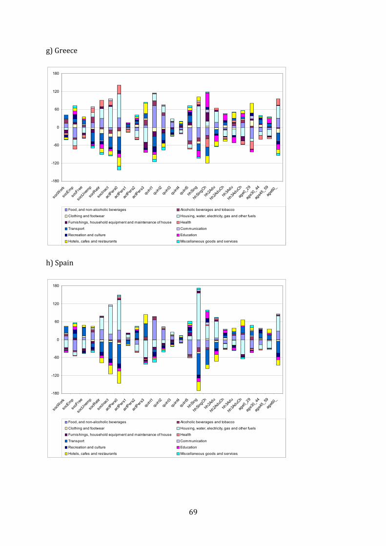
g) Greece

-180

-120

-60

0

60

120

180

socW

ork

socE

mp

socF

ree

socU

nemp

socR

etir

socIn

act

actPers

0

actPers

1

actPers

2

actPers

3qu

int1qu

int2qu

int3qu

int4qu

int5

hhSing

hhSing

Ch

hh2A

du

hh2A

duCh

hh3A

du

hh3A

duCh

age0

_29

age3

0_44

age4

5_59

age6

0_

Food, and non-alcoholic beverages Alcoholic beverages and tobacco

Clothing and footwear Housing, water, electricity, gas and other fuels

Furnishings, household equipment and maintenance of house Health

Transport Communication

Recreation and culture Education

69

Hotels, cafes and restaurants Miscellaneous goods and services h) Spain

-180

-120

-60

0

60

120

180

socW

ork

socE

mp

socF

ree

socU

nemp

socR

etir

socIn

act

actPers

0

actPers

1

actPers

2

actPers

3qu

int1qu

int2qu

int3qu

int4qu

int5

hhSing

hhSing

Ch

hh2A

du

hh2A

duCh

hh3A

du

hh3A

duCh

age0

_29

age3

0_44

age4

5_59

age6

0_

Food, and non-alcoholic beverages Alcoholic beverages and tobacco

Clothing and footwear Housing, water, electricity, gas and other fuels

Furnishings, household equipment and maintenance of house Health

Transport Communication

Recreation and culture Education

Hotels, cafes and restaurants Miscellaneous goods and services

i) France

-180

-120

-60

0

60

120

180

socW

ork

socE

mp

socF

ree

socU

nemp

socR

etir

socIn

act

actPers

0

actPers

1

actPers

2

actPers

3qu

int1qu

int2qu

int3qu

int4qu

int5

hhSing

hhSing

Ch

hh2A

du

hh2A

duCh

hh3A

du

hh3A

duCh

age0

_29

age3

0_44

age4

5_59

age6

0_

Food, and non-alcoholic beverages Alcoholic beverages and tobacco

Clothing and footwear Housing, water, electricity, gas and other fuels

Furnishings, household equipment and maintenance of house Health

Transport Communication

Recreation and culture Education

70

Hotels, cafes and restaurants Miscellaneous goods and services j) Italy

-180

-120

-60

0

60

120

180

socW

ork

socE

mp

socF

ree

socU

nemp

socR

etir

socIn

act

actPers

0

actPers

1

actPers

2

actPers

3qu

int1qu

int2qu

int3qu

int4qu

int5

hhSing

hhSing

Ch

hh2A

du

hh2A

duCh

hh3A

du

hh3A

duCh

age0

_29

age3

0_44

age4

5_59

age6

0_

Food, and non-alcoholic beverages Alcoholic beverages and tobacco

Clothing and footwear Housing, water, electricity, gas and other fuels

Furnishings, household equipment and maintenance of house Health

Transport Communication

Recreation and culture Education

Hotels, cafes and restaurants Miscellaneous goods and services

k) Luxemburg

-180

-120

-60

0

60

120

180

socW

ork

socE

mp

socF

ree

socU

nemp

socR

etir

socIn

act

actPers

0

actPers

1

actPers

2

actPers

3qu

int1qu

int2qu

int3qu

int4qu

int5

hhSing

hhSing

Ch

hh2A

du

hh2A

duCh

hh3A

du

hh3A

duCh

age0

_29

age3

0_44

age4

5_59

age6

0_

Food, and non-alcoholic beverages Alcoholic beverages and tobacco

Clothing and footwear Housing, water, electricity, gas and other fuels

Furnishings, household equipment and maintenance of house Health

Transport Communication

Recreation and culture Education

71

Hotels, cafes and restaurants Miscellaneous goods and services l) Netherlands

-180

-120

-60

0

60

120

180

socW

ork

socE

mp

socF

ree

socU

nemp

socR

etir

socIn

act

actPers

0

actPers

1

actPers

2

actPers

3qu

int1qu

int2qu

int3qu

int4qu

int5

hhSing

hhSing

Ch

hh2A

du

hh2A

duCh

hh3A

du

hh3A

duCh

age0

_29

age3

0_44

age4

5_59

age6

0_

Food, and non-alcoholic beverages Alcoholic beverages and tobacco

Clothing and footwear Housing, water, electricity, gas and other fuels

Furnishings, household equipment and maintenance of house Health

Transport Communication

Recreation and culture Education

Hotels, cafes and restaurants Miscellaneous goods and services

m) Austria

-180

-120

-60

0

60

120

180

socW

ork

socE

mp

socF

ree

socU

nemp

socR

etir

socIn

act

actPers

0

actPers

1

actPers

2

actPers

3qu

int1qu

int2qu

int3qu

int4qu

int5

hhSing

hhSing

Ch

hh2A

du

hh2A

duCh

hh3A

du

hh3A

duCh

age0

_29

age3

0_44

age4

5_59

age6

0_

Food, and non-alcoholic beverages Alcoholic beverages and tobacco

Clothing and footwear Housing, water, electricity, gas and other fuels

Furnishings, household equipment and maintenance of house Health

Transport Communication

Recreation and culture Education

72

Hotels, cafes and restaurants Miscellaneous goods and services n) Portugal

-180

-120

-60

0

60

120

180

socW

ork

socE

mp

socF

ree

socU

nemp

socR

etir

socIn

act

actPers

0

actPers

1

actPers

2

actPers

3qu

int1qu

int2qu

int3qu

int4qu

int5

hhSing

hhSing

Ch

hh2A

du

hh2A

duCh

hh3A

du

hh3A

duCh

age0

_29

age3

0_44

age4

5_59

age6

0_

Food, and non-alcoholic beverages Alcoholic beverages and tobacco

Clothing and footwear Housing, water, electricity, gas and other fuels

Furnishings, household equipment and maintenance of house Health

Transport Communication

Recreation and culture Education

Hotels, cafes and restaurants Miscellaneous goods and services

o) Finland

-180

-120

-60

0

60

120

180

socW

ork

socE

mp

socF

ree

socU

nemp

socR

etir

socIn

act

actPers

0

actPers

1

actPers

2

actPers

3qu

int1qu

int2qu

int3qu

int4qu

int5

hhSing

hhSing

Ch

hh2A

du

hh2A

duCh

hh3A

du

hh3A

duCh

age0

_29

age3

0_44

age4

5_59

age6

0_

Food, and non-alcoholic beverages Alcoholic beverages and tobacco

Clothing and footwear Housing, water, electricity, gas and other fuels

Furnishings, household equipment and maintenance of house Health

Transport Communication

Recreation and culture Education

73

Hotels, cafes and restaurants Miscellaneous goods and services p) Sweden

-180

-120

-60

0

60

120

180

socW

ork

socE

mp

socF

ree

socU

nemp

socR

etir

socIn

act

actPers

0

actPers

1

actPers

2

actPers

3qu

int1qu

int2qu

int3qu

int4qu

int5

hhSing

hhSing

Ch

hh2A

du

hh2A

duCh

hh3A

du

hh3A

duCh

age0

_29

age3

0_44

age4

5_59

age6

0_

Food, and non-alcoholic beverages Alcoholic beverages and tobacco

Clothing and footwear Housing, water, electricity, gas and other fuels

Furnishings, household equipment and maintenance of house Health

Transport Communication

Recreation and culture Education

Hotels, cafes and restaurants Miscellaneous goods and services

q) United Kingdom

-180

-120

-60

0

60

120

180

socW

ork

socE

mp

socF

ree

socU

nemp

socR

etir

socIn

act

actPers

0

actPers

1

actPers

2

actPers

3qu

int1qu

int2qu

int3qu

int4qu

int5

hhSing

hhSing

Ch

hh2A

du

hh2A

duCh

hh3A

du

hh3A

duCh

age0

_29

age3

0_44

age4

5_59

age6

0_

Food, and non-alcoholic beverages Alcoholic beverages and tobacco

Clothing and footwear Housing, water, electricity, gas and other fuels

Furnishings, household equipment and maintenance of house Health

Transport Communication

Recreation and culture Education

Hotels, cafes and restaurants Miscellaneous goods and services Note: The abbreviations used in the figures above and other figures are explained in detail in the Appendix (tables b.A.1-3, pp. 132f.). At this stage, we can form a hypothesis: looking at disaggregated data in section a), we find that prices of some product groups, mainly in the service sector, exhibit significant price increases during the euro introduction. Specifically, these categories are “Catering services”, “Cleaning, repair and hire of clothing”, “Hairdressing salons and personal grooming establishments”, “Repair of audio-visual, photographic and information proc-essing equipment” and “Operation of personal transport equipment”. Therefore, house-holds with a "larger-than-average" weight in these categories – typically higher-income households, households with several active persons involved in the labour market – should be prone to cash changeover related inflation effects. b.2.2) Changes in aggregate consumption structure over time Shifts in the aggregate consumption structure influence household-specific inflation rates, too. Figure b.2 plots the fractions of different categories according to the relatively rough COICOP level 2 classification (see appendix) in all countries under investigation to make general trends visible (in per mille the weights always sum up to 1000).

74

There are several common trends all over Europe and some (minor) exceptions: • First, the portion spent on food (incl. non-alcoholic beverages), but also on al-coholic beverages and tobacco, is steadily declining all over Europe. A common trend behind this seems to be the steady increase of average per capita income in most countries, intensified by a shift in preferences towards a more healthy lifestyle in a couple of countries.

75

• Second, the share spent on clothing and footwear decreases, while the expendi-ture share for housing, electricity, gas and fuels is roughly constant – perhaps reflecting to an extent the increase in oil prices over the analysed time period. The share spent on transport is also roughly constant. • Third, the shares spent on health are increasing in most countries – but still the weight is low on an aggregate level. • Fourth, in a number of countries, the share spent on hotel and restaurant ser-vices has increased.

Figure b.2 Weights for the 12 COICOP groups in aggregate consumption over time for EU 15 and Euro area member

76

0

200

400

600

800

1000

96 97 98 99 00 01 02 03 04 05 06

AT_C P1AT_C P2AT_C P3AT_C P4

AT_C P5AT_C P6AT_C P7AT_C P8

AT_C P9AT_C P10AT_C P11AT_C P12

0

200

400

600

800

1000

96 97 98 99 00 01 02 03 04 05 06

BE_C P1BE_C P2BE_C P3BE_C P4

BE_C P5BE_C P6BE_C P7BE_C P8

BE_C P9BE_C P10BE_C P11BE_C P12

0

200

400

600

800

1000

96 97 98 99 00 01 02 03 04 05 06

D E_C P1D E_C P2D E_C P3D E_C P4

D E_C P5D E_C P6D E_C P7D E_C P8

D E_C P9D E_C P10D E_C P11D E_C P12

0

200

400

600

800

1000

96 97 98 99 00 01 02 03 04 05 06

D K_C P1D K_C P2D K_C P3D K_C P4

D K_C P5D K_C P6D K_C P7D K_C P8

D K_C P9D K_C P10D K_C P11D K_C P12

0

200

400

600

800

1000

96 97 98 99 00 01 02 03 04 05 06

EA_C P1EA_C P2EA_C P3EA_C P4

EA_C P5EA_C P6EA_C P7EA_C P8

EA_C P9EA_C P10EA_C P11EA_C P12

0

200

400

600

800

1000

96 97 98 99 00 01 02 03 04 05 06

ES_C P1ES_C P2ES_C P3ES_C P4

ES_C P5ES_C P6ES_C P7ES_C P8

ES_C P9ES_C P10ES_C P11ES_C P12

0

200

400

600

800

1000

96 97 98 99 00 01 02 03 04 05 06

EU 15_C P1EU 15_C P2EU 15_C P3EU 15_C P4

EU 15_C P5EU 15_C P6EU 15_C P7EU 15_C P8

EU 15_C P9EU 15_C P10EU 15_C P11EU 15_C P12

0

200

400

600

800

1000

96 97 98 99 00 01 02 03 04 05 06

FI_C P1FI_C P2FI_C P3FI_C P4

FI_C P5FI_C P6FI_C P7FI_C P8

FI_C P9FI_C P10FI_C P11FI_C P12

0

200

400

600

800

1000

96 97 98 99 00 01 02 03 04 05 06

FR _C P1FR _C P2FR _C P3FR _C P4

FR _C P5FR _C P6FR _C P7FR _C P8

FR _C P9FR _C P10FR _C P11FR _C P12

0

200

400

600

800

1000

96 97 98 99 00 01 02 03 04 05 06

GR _C P1GR _C P2GR _C P3GR _C P4

GR _C P5GR _C P6GR _C P7GR _C P8

GR _C P9GR _C P10GR _C P11GR _C P12

0

200

400

600

800

1000

96 97 98 99 00 01 02 03 04 05 06

IE_C P1IE_C P2IE_C P3IE_C P4

IE_C P5IE_C P6IE_C P7IE_C P8

IE_C P9IE_C P10IE_C P11IE_C P12

0

200

400

600

800

1000

96 97 98 99 00 01 02 03 04 05 06

IT_C P1IT_C P2IT_C P3IT_C P4

IT_C P5IT_C P6IT_C P7IT_C P8

IT_C P9IT_C P10IT_C P11IT_C P12

0

200

400

600

800

1000

96 97 98 99 00 01 02 03 04 05 06

LU _C P1LU _C P2LU _C P3LU _C P4

LU _C P5LU _C P6LU _C P7LU _C P8

LU _C P9LU _C P10LU _C P11LU _C P12

0

200

400

600

800

1000

96 97 98 99 00 01 02 03 04 05 06

N L_C P1N L_C P2N L_C P3N L_C P4

N L_C P5N L_C P6N L_C P7N L_C P8

N L_C P9N L_C P10N L_C P11N L_C P12

0

200

400

600

800

1000

96 97 98 99 00 01 02 03 04 05 06

PT_C P1PT_C P2PT_C P3PT_C P4

PT_C P5PT_C P6PT_C P7PT_C P8

PT_C P9PT_C P10PT_C P11PT_C P12

0

200

400

600

800

1000

96 97 98 99 00 01 02 03 04 05 06

SE_C P1SE_C P2SE_C P3SE_C P4

SE_C P5SE_C P6SE_C P7SE_C P8

SE_C P9SE_C P10SE_C P11SE_C P12

0

200

400

600

800

1000

96 97 98 99 00 01 02 03 04 05 06

U K_C P1U K_C P2U K_C P3U K_C P4

U K_C P5U K_C P6U K_C P7U K_C P8

U K_C P9U K_C P10U K_C P11U K_C P12

77

b.3) Simulations of price developments We compute household-specific price indices for all categories for which this is reasona-bly possible (filling empty cells by adding-up constraints if this is possible). Overall, we end up with 363 time series. To keep the headers of the time series short in presentation and calculation, we use a system of descriptors where the first part (SOC, ACT, QUINT, HH, … ) refers to the household categories we use (see section b.2.1), whereas the sec-ond part refers to subcategories. A complete overview of all time series and a list of de-scriptors can be found in the appendix. In this section, we analyse household-specific inflation rates expressed as deviations from the overall inflation rate as measured by the aggregate consumer price level (in percentage points). This procedure is in line with the hypothesis that household-specific effects matter insofar as certain households are affected differently from the median household (whose consumption pattern should provide the basis for the construction of a representative basket; see section b.2.1 for the implicit ‘middle-class’ bias observable in the data). Overall, we find that the inflation rates are quite similar in the overwhelm-ing majority of countries and deviations appear to be low. To get an impression how large the deviations are across Europe and whether developments for Euro area coun-tries differ from those in non-Euro area countries, we present cross-household-type standard deviations for each country at any point in time on the same scale (left); figures are shown below:8

8 One could argue that our 25 categories do not cover the income distribution or socio-economic charac-teristics of a country in a representative way. However, since we use the same categories for all countries, the error should not matter much.

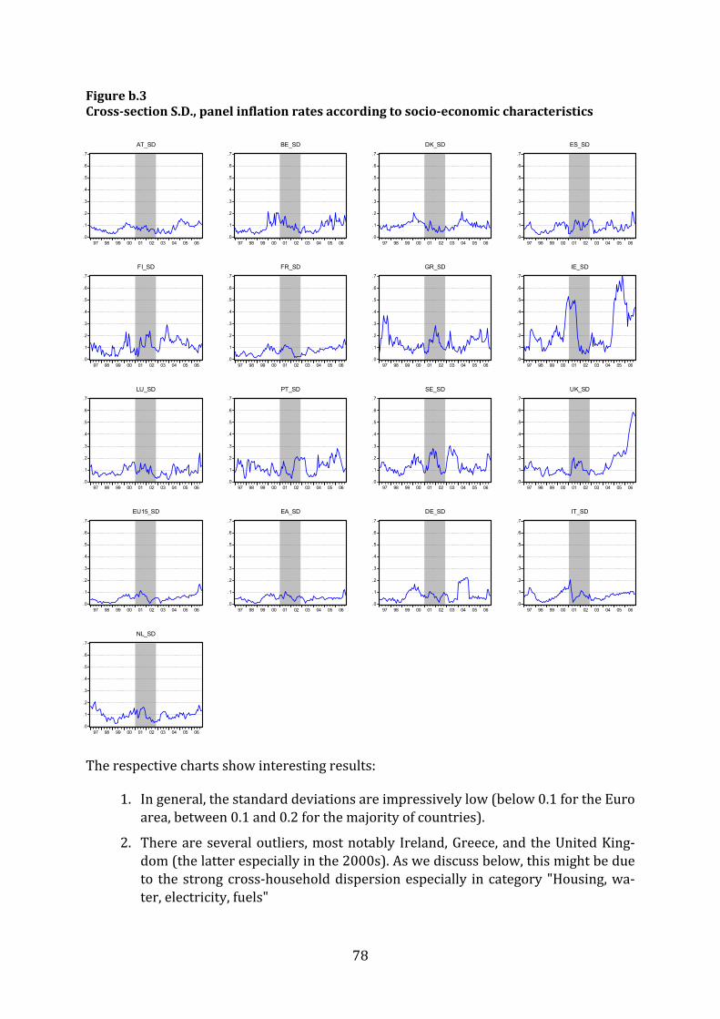
Figure b.3 Cross-section S.D., panel inflation rates according to socio-economic characteristics

.0

.1

.2

.3

.4

.5

.6

.7

97 98 99 00 01 02 03 04 05 06

AT_SD

.0

.1

.2

.3

.4

.5

.6

.7

97 98 99 00 01 02 03 04 05 06

BE_SD

.0

.1

.2

.3

.4

.5

.6

.7

97 98 99 00 01 02 03 04 05 06

DK_SD

.0

.1

.6

78

.2

.3

.4

.5

.7

97 98 99 00 01 02 03 04 05 06

ES_SD

.0

.1

.2

.3

.4

.5

.6

.7

97 98 99 00 01 02 03 04 05 06

FI_SD

.0

.1

.2

.3

.4

.5

.6

.7

97 98 99 00 01 02 03 04 05 06

FR_SD

.0

.1

.2

.3

.4

.5

.6

.7

97 98 99 00 01 02 03 04 05 06

GR_SD

.0

.1

.2

.3

.4

.5

.6

.7

97 98 99 00 01 02 03 04 05 06

IE_SD

.0

.1

.2

.3

.4

.5

.6

.7

97 98 99 00 01 02 03 04 05 06

LU_SD

.0

.1

.2

.3

.4

.5

.6

.7

97 98 99 00 01 02 03 04 05 06

PT_SD

.0

.1

.2

.3

.4

.5

.6

.7

97 98 99 00 01 02 03 04 05 06

SE_SD

.0

.1

.6

.2

.3

.4

.5

.7

97 98 99 00 01 02 03 04 05 06

UK_SD

.0

.1

.2

.3

.4

.5

.6

.7

97 98 99 00 01 02 03 04 05 06

EU15_SD

.0

.1

.2

.3

.4

.5

.6

.7

97 98 99 00 01 02 03 04 05 06

EA_SD

.0

.1

.2

.3

.4

.5

.6

.7

97 98 99 00 01 02 03 04 05 06

DE_SD

.0

.1

.6

.2

.3

.4

.5

.7

97 98 99 00 01 02 03 04 05 06

IT_SD

.0

.1

.2

.3

.4

.5

.6

.7

97 98 99 00 01 02 03 04 05 06

NL_SD

T espective charts show interesting results: 1. In general, the standard deviations are impressively low (below 0.1 for the Euro he rarea, between 0.1 and 0.2 for the majority of countries). 2. There are several outliers, most notably Ireland, Greece, and the United King-dom (the latter especially in the 2000s). As we discuss below, this might be due to the strong cross-household dispersion especially in category "Housing, wa-ter, electricity, fuels"

79

3. There is an increase in the dispersion of inflation rates around 2001/2002. However, this increase is also visible in Sweden and United Kingdom as well, suggesting a non-Euro related explanation. (For instance, food prices increased outh of Europe, oil price increase etc.). in 2001 due to bad harvests in the sLet us now turn to a more detailed analysis: • First, the left graph of Figure b.4 shows a complete overview of all deviations from the HICP for all countries over time to get an impression for the phe-nomenon across countries and across time. • Second, to get an idea for which socio-economic factors the deviations are more pronounced and to find out whether there are individual inflation rates which differ systematically, an easy-to-interpret graphical tool is used, the Box-Whisker-Plot.9 The Box-Whisker-Plot summarizes information on the distribu-tion of the respective series (first, second, and even third moments) and makes a panel of distributions comparable. For the overall sample, this plot is shown in the middle of Figure b.4. • Third, to analyze the effects around the euro changeover, we use again the Box-Whisker-Plots but only for the period from 2001m1 to 2002m12 (to cover the period before the changeover, which many people claim to be ’infected‘ as well).

9 The median is plotted by a line in the centre of a box together with shaded areas denoting a significance area, a box denoting the borders to the first and third quartile, and a whisker denoting the inner fences (1.5 times the interquartile range). Data points with a circle denote near outliers, stars indicate a far out-lier.

Figure b.4 s from HICP (left), Box-Whisker-plots (full sample, middle) and Box-Whisker-plot (2001–2002, right) Deviationa) EU 15

-.3

-.2

-.1

.0

.1

.2

.3

.4

97 98 99 00 01 02 03 04 05 06

EU15_SOCWORKEU15_SOCFREEEU15_SOCINACTEU15_ACTPERS0EU15_ACTPERS1EU15_ACTPERS2EU15_ACTPERS3

EU15_QUINT1EU15_QUINT2EU15_QUINT3EU15_QUINT4EU15_QUINT5EU15_HHSINGEU15_HHSINGCH

EU15_HH2ADUEU15_HH2ADUCHEU15_HH3ADUEU15_AGE0EU15_AGE30EU15_AGE45EU15_AGE60

-.3

-.2

-.1

.0

.1

.2

.3

.4

EU

15_SOC

WO

RK

EU

15_SOC

FRE

EE

U15_SO

CIN

ACT

EU

15_ACTP

ER

S0

EU

15_ACTP

ER

S1

EU

15_ACTP

ER

S2

EU

15_ACTP

ER

S3

EU

15_QU

INT1

EU

15_QU

INT2

EU

15_QU

INT3

EU

15_QU

INT4

EU

15_QU

INT5

EU

15_HH

SIN

GE

U15_H

HS

ING

CH

EU

15_HH

2AD

UE

U15_H

H2A

DU

CH

EU

15_HH

3AD

UE

U15_AG

E0

EU

15_AGE

30E

U15_AG

E45

EU

15_AGE

60 -.12

-.08

-.04

.00

.04

.08

.12

EU

15_SO

CW

OR

KE

U15_S

OC

FRE

EE

U15_S

OC

INA

CT

EU

15_AC

TPE

RS

0E

U15_A

CTP

ER

S1

EU

15_AC

TPE

RS

2E

U15_A

CTP

ER

S3

EU

15_QU

INT1

EU

15_QU

INT2

EU

15_QU

INT3

EU

15_QU

INT4

EU

15_QU

INT5

EU

15_HH

SIN

GE

U15_H

HS

ING

CH

EU

15_HH

2AD

UE

U15_H

H2A

DU

CH

EU

15_HH

3AD

UE

U15_A

GE

0E

U15_A

GE

30E

U15_A

GE

45E

U15_A

GE

60

80

b) Euro area

-.3

-.2

-.1

.0

.1

.2

.3

97 98 99 00 01 02 03 04 05 06

EA_SOCWORKEA_SOCFREEEA_SOCINACTEA_ACTPERS0EA_ACTPERS1EA_ACTPERS2EA_ACTPERS3EA_QUINT1

EA_QUINT2EA_QUINT3EA_QUINT4EA_QUINT5EA_HHSINGEA_HHSINGCHEA_HH2ADUEA_HH2ADUCH

EA_HH3ADUEA_HH3ADUCHEA_AGE0EA_AGE30EA_AGE45EA_AGE60

-.3

-.2

-.1

.0

.1

.2

.3

EA

_SO

CW

OR

KE

A_S

OC

FREE

EA

_SO

CIN

AC

TE

A_A

CTPE

RS

0E

A_A

CTPE

RS

1E

A_A

CTPE

RS

2E

A_A

CTPE

RS

3E

A_Q

UIN

T1E

A_Q

UIN

T2E

A_Q

UIN

T3E

A_Q

UIN

T4E

A_Q

UIN

T5E

A_H

HS

ING

EA

_HH

SIN

GC

HE

A_H

H2AD

UE

A_H

H2AD

UC

HE

A_H

H3AD

UE

A_H

H3AD

UC

HE

A_A

GE

0E

A_A

GE

30E

A_A

GE

45E

A_A

GE

60 -.10

-.05

.00

.05

.10

.15

EA_SO

CW

OR

KE

A_SOC

FREE

EA_SO

CIN

AC

TE

A_ACTP

ERS

0E

A_ACTP

ERS

1E

A_ACTP

ERS

2E

A_ACTP

ERS

3E

A_QU

INT1

EA_Q

UIN

T2E

A_QU

INT3

EA_Q

UIN

T4E

A_QU

INT5

EA_H

HSIN

GE

A_HH

SING

CH

EA_H

H2A

DU

EA_H

H2A

DU

CH

EA_H

H3A

DU

EA_H

H3A

DU

CH

EA_AG

E0E

A_AGE30

EA_AG

E45E

A_AGE60

81

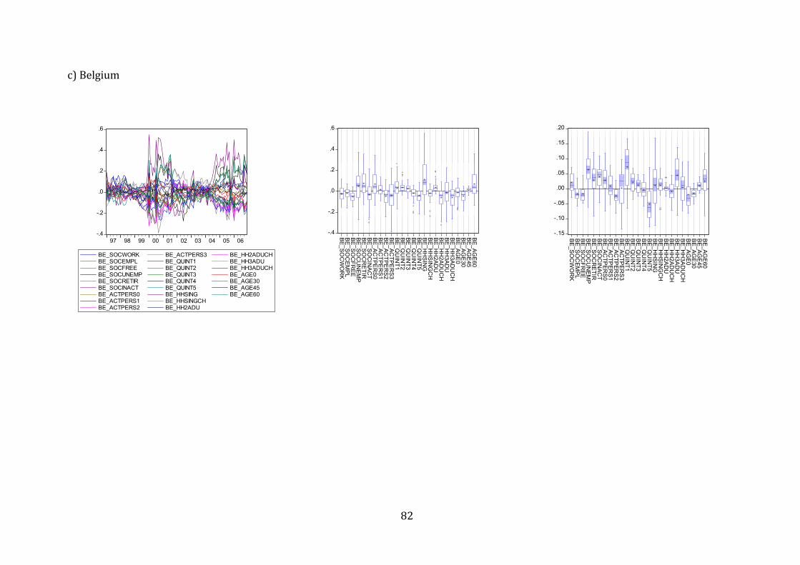
c) Belgium

-.4

-.2

.0

.2

.4

.6

97 98 99 00 01 02 03 04 05 06

BE_SOCWORKBE_SOCEMPLBE_SOCFREEBE_SOCUNEMPBE_SOCRETIRBE_SOCINACTBE_ACTPERS0BE_ACTPERS1BE_ACTPERS2

BE_ACTPERS3BE_QUINT1BE_QUINT2BE_QUINT3BE_QUINT4BE_QUINT5BE_HHSINGBE_HHSINGCHBE_HH2ADU

BE_HH2ADUCHBE_HH3ADUBE_HH3ADUCHBE_AGE0BE_AGE30BE_AGE45BE_AGE60

-.4

-.2

.0

.2

.4

.6

BE

_SO

CW

OR

KB

E_S

OC

EM

PL

BE

_SO

CFR

EE

BE

_SO

CU

NE

MP

BE

_SO

CR

ETIR

BE

_SO

CIN

AC

TB

E_A

CTP

ER

S0

BE

_AC

TPE

RS

1B

E_A

CTP

ER

S2

BE

_AC

TPE

RS

3B

E_Q

UIN

T1B

E_Q

UIN

T2B

E_Q

UIN

T3B

E_Q

UIN

T4B

E_Q

UIN

T5B

E_H

HS

ING

BE

_HH

SIN

GC

HB

E_H

H2A

DU

BE

_HH

2AD

UC

HB

E_H

H3A

DU

BE

_HH

3AD

UC

HB

E_A

GE

0B

E_A

GE

30B

E_A

GE

45B

E_A

GE

60 -.15

-.10

-.05

.00

.05

.10

.15

.20

BE

_SO

CW

OR

KB

E_S

OC

EMP

LB

E_S

OC

FREE

BE

_SO

CU

NEM

PB

E_S

OC

RETIR

BE

_SO

CIN

AC

TB

E_A

CTP

ERS

0B

E_A

CTP

ERS

1B

E_A

CTP

ERS

2B

E_A

CTP

ERS

3B

E_Q

UIN

T1B

E_Q

UIN

T2B

E_Q

UIN

T3B

E_Q

UIN

T4B

E_Q

UIN

T5B

E_H

HS

ING

BE

_HH

SIN

GC

HB

E_H

H2A

DU

BE

_HH

2AD

UC

HB

E_H

H3A

DU

BE

_HH

3AD

UC

HB

E_A

GE

0B

E_A

GE

30B

E_A

GE

45B

E_A

GE

60

82

d) Denmark

-.6

-.4

-.2

.0

.2

.4

97 98 99 00 01 02 03 04 05 06

DK_SOCWORKDK_SOCEMPLDK_SOCFREEDK_SOCUNEMPDK_SOCRETIRDK_SOCINACTDK_ACTPERS0DK_ACTPERS1DK_ACTPERS2

DK_ACTPERS3DK_QUINT1DK_QUINT2DK_QUINT3DK_QUINT4DK_QUINT5DK_HHSINGDK_HHSINGCHDK_HH2ADU

DK_HH2ADUCHDK_HH3ADUDK_HH3ADUCHDK_AGE0DK_AGE30DK_AGE45DK_AGE60

-.6

-.4

-.2

.0

.2

.4

DK

_SO

CW

OR

KD

K_S

OC

EM

PLD

K_S

OC

FRE

ED

K_S

OC

UN

EM

PD

K_S

OC

RE

TIRD

K_S

OC

INAC

TD

K_A

CTP

ER

S0D

K_A

CTP

ER

S1D

K_A

CTP

ER

S2D

K_A

CTP

ER

S3D

K_Q

UIN

T1D

K_Q

UIN

T2D

K_Q

UIN

T3D

K_Q

UIN

T4D

K_Q

UIN

T5D

K_H

HSIN

GD

K_H

HSIN

GC

HD

K_H

H2A

DU

DK

_HH

2AD

UC

HD

K_H

H3A

DU

DK

_HH

3AD

UC

HD

K_A

GE0

DK

_AG

E30D

K_A

GE45

DK

_AG

E60 -.3

-.2

-.1

.0

.1

.2

DK

_SO

CW

OR

KD

K_S

OC

EM

PLD

K_S

OC

FRE

ED

K_S

OC

UN

EM

PD

K_S

OC

RE

TIRD

K_S

OC

INAC

TD

K_A

CTP

ER

S0D

K_A

CTP

ER

S1D

K_A

CTP

ER

S2D

K_A

CTP

ER

S3D

K_Q

UIN

T1D

K_Q

UIN

T2D

K_Q

UIN

T3D

K_Q

UIN

T4D

K_Q

UIN

T5D

K_H

HSIN

GD

K_H

HSIN

GC

HD

K_H

H2A

DU

DK

_HH

2AD

UC

HD

K_H

H3A

DU

DK

_HH

3AD

UC

HD

K_A

GE0

DK

_AG

E30D

K_A

GE45

DK

_AG

E60

83

e) Germany

-.4

-.3

-.2

-.1

.0

.1

.2

.3

.4

.5

97 98 99 00 01 02 03 04 05 06

DE_SOCWORKDE_SOCFREEDE_SOCUNEMPDE_SOCINACTDE_ACTPERS0DE_ACTPERS1DE_ACTPERS2DE_ACTPERS3

DE_QUINT1DE_QUINT2DE_QUINT3DE_QUINT4DE_QUINT5DE_HHSINGDE_HHSINGCHDE_HH2ADU

DE_HH2ADUCHDE_HH3ADUDE_HH3ADUCHDE_AGE0DE_AGE30DE_AGE45DE_AGE60

-.4

-.3

-.2

-.1

.0

.1

.2

.3

.4

.5

DE

_SO

CW

OR

KD

E_S

OC

FRE

ED

E_S

OC

UN

EM

PD

E_S

OC

INAC

TD

E_A

CTP

ER

S0D

E_A

CTP

ER

S1D

E_A

CTP

ER

S2D

E_A

CTP

ER

S3D

E_Q

UIN

T1D

E_Q

UIN

T2D

E_Q

UIN

T3D

E_Q

UIN

T4D

E_Q

UIN

T5D

E_H

HSIN

GD

E_H

HSIN

GC

HD

E_H

H2A

DU

DE

_HH

2AD

UC

HD

E_H

H3A

DU

DE

_HH

3AD

UC

HD

E_A

GE0

DE

_AG

E30D

E_A

GE45

DE

_AG

E60 -.15

-.10

-.05

.00

.05

.10

.15

DE

_SO

CW

OR

KD

E_S

OC

FRE

ED

E_S

OC

UN

EM

PD

E_S

OC

INAC

TD

E_A

CTPE

RS

0D

E_A

CTPE

RS

1D

E_A

CTPE

RS

2D

E_A

CTPE

RS

3D

E_Q

UIN

T1D

E_Q

UIN

T2D

E_Q

UIN

T3D

E_Q

UIN

T4D

E_Q

UIN

T5D

E_H

HS

ING

DE

_HH

SIN

GC

HD

E_H

H2AD

UD

E_H

H2AD

UC

HD

E_H

H3AD

UD

E_H

H3AD

UC

HD

E_A

GE

0D

E_A

GE

30D

E_A

GE

45D

E_A

GE

60

84

f) Ireland

-1.0

-0.5

0.0

0.5

1.0

1.5

2.0

97 98 99 00 01 02 03 04 05 06

IE_SOCWORKIE_SOCEMPLIE_SOCFREEIE_SOCUNEMPIE_SOCRETIRIE_SOCINACTIE_ACTPERS0IE_ACTPERS1IE_ACTPERS2

IE_ACTPERS3IE_QUINT1IE_QUINT2IE_QUINT3IE_QUINT4IE_QUINT5IE_HHSINGIE_HHSINGCHIE_HH2ADU

IE_HH2ADUCHIE_HH3ADUIE_HH3ADUCHIE_AGE0IE_AGE30IE_AGE45IE_AGE60

-1.0

-0.5

0.0

0.5

1.0

1.5

2.0

IE_SO

CW

OR

KIE

_SOC

EM

PL

IE_SO

CFR

EEIE

_SOC

UN

EMP

IE_SO

CR

ETIR

IE_SO

CIN

AC

TIE

_ACTP

ER

S0

IE_AC

TPE

RS

1IE

_ACTP

ER

S2

IE_AC

TPE

RS

3IE

_QU

INT1

IE_Q

UIN

T2IE

_QU

INT3

IE_Q

UIN

T4IE

_QU

INT5

IE_H

HS

ING

IE_H

HS

ING

CH

IE_H

H2A

DU

IE_H

H2A

DU

CH

IE_H

H3A

DU

IE_H

H3A

DU

CH

IE_AG

E0

IE_AG

E30

IE_AG

E45

IE_AG

E60

-.8

-.6

-.4

-.2

.0

.2

.4

IE_SO

CW

OR

KIE

_SOC

EM

PL

IE_SO

CFR

EEIE

_SOC

UN

EMP

IE_SO

CR

ETIR

IE_SO

CIN

AC

TIE

_ACTP

ER

S0

IE_AC

TPE

RS

1IE

_ACTP

ER

S2

IE_AC

TPE

RS

3IE

_QU

INT1

IE_Q

UIN

T2IE

_QU

INT3

IE_Q

UIN

T4IE

_QU

INT5

IE_H

HS

ING

IE_H

HS

ING

CH

IE_H

H2A

DU

IE_H

H2A

DU

CH

IE_H

H3A

DU

IE_H

H3A

DU

CH

IE_AG

E0

IE_AG

E30

IE_AG

E45

IE_AG

E60

85

g) Greece

-1.2

-0.8

-0.4

0.0

0.4

0.8

97 98 99 00 01 02 03 04 05 06

GR_SOCWORKGR_SOCEMPLGR_SOCFREEGR_SOCUNEMPGR_SOCRETIRGR_SOCINACTGR_ACTPERS0GR_ACTPERS1GR_ACTPERS2

GR_ACTPERS3GR_QUINT1GR_QUINT2GR_QUINT3GR_QUINT4GR_QUINT5GR_HHSINGGR_HHSINGCHGR_HH2ADU

GR_HH2ADUCHGR_HH3ADUGR_HH3ADUCHGR_AGE0GR_AGE30GR_AGE45GR_AGE60

-1.2

-0.8

-0.4

0.0

0.4

0.8

GR

_SO

CW

OR

KG

R_S

OC

EM

PLG

R_S

OC

FRE

EG

R_S

OC

UN

EM

PG

R_S

OC

RE

TIRG

R_S

OC

INAC

TG

R_A

CTP

ER

S0G

R_A

CTP

ER

S1G

R_A

CTP

ER

S2G

R_A

CTP

ER

S3G

R_Q

UIN

T1G

R_Q

UIN

T2G

R_Q

UIN

T3G

R_Q

UIN

T4G

R_Q

UIN

T5G

R_H

HSIN

GG

R_H

HSIN

GC

HG

R_H

H2A

DU

GR

_HH

2AD

UC

HG

R_H

H3A

DU

GR

_HH

3AD

UC

HG

R_A

GE0

GR

_AG

E30G

R_A

GE45

GR

_AG

E60 -1.2

-0.8

-0.4

0.0

0.4

0.8

GR

_SO

CW

OR

KG

R_S

OC

EM

PLG

R_S

OC

FRE

EG

R_S

OC

UN

EM

PG

R_S

OC

RE

TIRG

R_S

OC

INAC

TG

R_A

CTP

ER

S0G

R_A

CTP

ER

S1G

R_A

CTP

ER

S2G

R_A

CTP

ER

S3G

R_Q

UIN

T1G

R_Q

UIN

T2G

R_Q

UIN

T3G

R_Q

UIN

T4G

R_Q

UIN

T5G

R_H

HSIN

GG

R_H

HSIN

GC

HG

R_H

H2A

DU

GR

_HH

2AD

UC

HG

R_H

H3A

DU

GR

_HH

3AD

UC

HG

R_A

GE0

GR

_AG

E30G

R_A

GE45

GR

_AG

E60

86

h) Spain

-.6

-.4

-.2

.0

.2

.4

.6

97 98 99 00 01 02 03 04 05 06

ES_SOCWORKES_SOCEMPLES_SOCFREEES_SOCUNEMPES_SOCRETIRES_SOCINACTES_ACTPERS0ES_ACTPERS1ES_ACTPERS2

ES_ACTPERS3ES_QUINT1ES_QUINT2ES_QUINT3ES_QUINT4ES_QUINT5ES_HHSINGES_HHSINGCHES_HH2ADU

ES_HH2ADUCHES_HH3ADUES_HH3ADUCHES_AGE0ES_AGE30ES_AGE45ES_AGE60

-.6

-.4

-.2

.0

.2

.4

.6

ES

_SO

CW

OR

KE

S_S

OC

EM

PL

ES

_SO

CFR

EE

ES

_SO

CU

NE

MP

ES

_SO

CR

ETIR

ES

_SO

CIN

AC

TE

S_A

CTP

ER

S0

ES

_AC

TPE

RS

1E

S_A

CTP

ER

S2

ES

_AC

TPE

RS

3E

S_Q

UIN

T1E

S_Q

UIN

T2E

S_Q

UIN

T3E

S_Q

UIN

T4E

S_Q

UIN

T5E

S_H

HS

ING

ES

_HH

SIN

GC

HE

S_H

H2A

DU

ES

_HH

2AD

UC

HE

S_H

H3A

DU

ES

_HH

3AD

UC

HE

S_A

GE

0E

S_A

GE

30E

S_A

GE

45E

S_A

GE

60 -.4

-.3

-.2

-.1

.0

.1

.2

.3

ES_SO

CW

OR

KE

S_SOC

EM

PL

ES_SO

CFR

EEE

S_SOC

UN

EMP

ES_SO

CR

ETIR

ES_SO

CIN

AC

TE

S_ACTP

ER

S0

ES_AC

TPE

RS

1E

S_ACTP

ER

S2

ES_AC

TPE

RS

3E

S_QU

INT1

ES_Q

UIN

T2E

S_QU

INT3

ES_Q

UIN

T4E

S_QU

INT5

ES_H

HS

ING

ES_H

HS

ING

CH

ES_H

H2A

DU

ES_H

H2A

DU

CH

ES_H

H3A

DU

ES_H

H3A

DU

CH

ES_AG

E0

ES_AG

E30

ES_AG

E45

ES_AG

E60

87

i) France

-.3

-.2

-.1

.0

.1

.2

.3

.4

97 98 99 00 01 02 03 04 05 06

FR_SOCWORKFR_SOCEMPLFR_SOCFREEFR_SOCUNEMPFR_SOCRETIRFR_SOCINACTFR_ACTPERS0FR_ACTPERS1FR_ACTPERS2

FR_ACTPERS3FR_QUINT1FR_QUINT2FR_QUINT3FR_QUINT4FR_QUINT5FR_HHSINGFR_HHSINGCHFR_HH2ADU

FR_HH2ADUCHFR_HH3ADUFR_HH3ADUCHFR_AGE0FR_AGE30FR_AGE45FR_AGE60

-.3

-.2

-.1

.0

.1

.2

.3

.4

FR_SO

CW

OR

KFR

_SO

CE

MP

LFR

_SOC

FREE

FR_SO

CU

NEM

PFR

_SOC

RE

TIRFR

_SOC

INA

CT

FR_AC

TPER

S0

FR_AC

TPER

S1

FR_AC

TPER

S2

FR_AC

TPER

S3

FR_Q

UIN

T1FR

_QU

INT2

FR_Q

UIN

T3FR

_QU

INT4

FR_Q

UIN

T5FR

_HH

SIN

GFR

_HH

SIN

GC

HFR

_HH

2AD

UFR

_HH

2AD

UC

HFR

_HH

3AD

UFR

_HH

3AD

UC

HFR

_AGE

0FR

_AGE

30FR

_AGE

45FR

_AGE

60 -.15

-.10

-.05

.00

.05

.10

.15

FR_S

OC

WO

RK

FR_S

OC

EMP

LFR

_SO

CFR

EEFR

_SO

CU

NEM

PFR

_SO

CR

ETIRFR

_SO

CIN

AC

TFR

_AC

TPER

S0

FR_A

CTP

ERS

1FR

_AC

TPER

S2

FR_A

CTP

ERS

3FR

_QU

INT1

FR_Q

UIN

T2FR

_QU

INT3

FR_Q

UIN

T4FR

_QU

INT5

FR_H

HS

ING

FR_H

HS

ING

CH

FR_H

H2A

DU

FR_H

H2A

DU

CH

FR_H

H3A

DU

FR_H

H3A

DU

CH

FR_A

GE

0FR

_AG

E30

FR_A

GE

45FR

_AG

E60

88

j) Italy

-.3

-.2

-.1

.0

.1

.2

.3

.4

97 98 99 00 01 02 03 04 05 06

IT_SOCWORKIT_SOCFREEIT_SOCUNEMPIT_SOCRETIRIT_SOCINACTIT_ACTPERS0IT_ACTPERS1IT_ACTPERS2

IT_ACTPERS3IT_QUINT1IT_QUINT2IT_QUINT3IT_QUINT4IT_QUINT5IT_HHSINGIT_HHSINGCH

IT_HH2ADUIT_HH2ADUCHIT_HH3ADUIT_HH3ADUCHIT_AGE0IT_AGE30IT_AGE45IT_AGE60

-.3

-.2

-.1

.0

.1

.2

.3

.4

IT_SO

CW

OR

KIT_S

OC

FRE

EIT_S

OC

UN

EM

PIT_S

OC

RE

TIRIT_S

OC

INA

CT

IT_AC

TPE

RS

0IT_A

CTP

ER

S1

IT_AC

TPE

RS

2IT_A

CTP

ER

S3

IT_QU

INT1

IT_QU

INT2

IT_QU

INT3

IT_QU

INT4

IT_QU

INT5

IT_HH

SIN

GIT_H

HS

ING

CH

IT_HH

2AD

UIT_H

H2A

DU

CH

IT_HH

3AD

UIT_H

H3A

DU

CH

IT_AG

E0IT_A

GE30

IT_AG

E45IT_A

GE60

-.3

-.2

-.1

.0

.1

.2

.3

.4

IT_SO

CW

OR

KIT_S

OC

FRE

EIT_S

OC

UN

EM

PIT_S

OC

RETIR

IT_SO

CIN

AC

TIT_A

CTP

ERS0

IT_AC

TPER

S1IT_A

CTP

ERS2

IT_AC

TPER

S3IT_Q

UIN

T1IT_Q

UIN

T2IT_Q

UIN

T3IT_Q

UIN

T4IT_Q

UIN

T5IT_H

HS

ING

IT_HH

SIN

GC

HIT_H

H2A

DU

IT_HH

2AD

UC

HIT_H

H3A

DU

IT_HH

3AD

UC

HIT_A

GE

0IT_A

GE

30IT_A

GE

45IT_A

GE

60

89

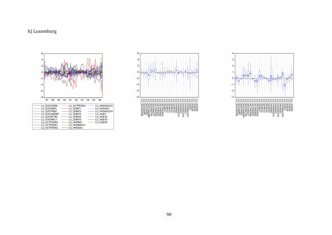
k) Luxemburg

-.8

-.6

-.4

-.2

.0

.2

.4

.6

97 98 99 00 01 02 03 04 05 06

LU_SOCWORKLU_SOCEMPLLU_SOCFREELU_SOCUNEMPLU_SOCRETIRLU_SOCINACTLU_ACTPERS0LU_ACTPERS1LU_ACTPERS2

LU_ACTPERS3LU_QUINT1LU_QUINT2LU_QUINT3LU_QUINT4LU_QUINT5LU_HHSINGLU_HHSINGCHLU_HH2ADU

LU_HH2ADUCHLU_HH3ADULU_HH3ADUCHLU_AGE0LU_AGE30LU_AGE45LU_AGE60

-.8

-.6

-.4

-.2

.0

.2

.4

.6

LU_S

OC

WO

RK

LU_S

OC

EM

PL

LU_S

OC

FRE

ELU

_SO

CU

NE

MP

LU_S

OC

RE

TIRLU

_SO

CIN

AC

TLU

_AC

TPE

RS0

LU_A

CTP

ER

S1LU

_AC

TPE

RS2

LU_A

CTP

ER

S3LU

_QU

INT1

LU_Q

UIN

T2LU

_QU

INT3

LU_Q

UIN

T4LU

_QU

INT5

LU_H

HSIN

GLU

_HH

SING

CH

LU_H

H2A

DU

LU_H

H2A

DU

CH

LU_H

H3A

DU

LU_H

H3A

DU

CH

LU_A

GE0

LU_A

GE30

LU_A

GE45

LU_A

GE60

-.3

-.2

-.1

.0

.1

.2

.3

.4

LU_S

OC

WO

RK

LU_S

OC

EM

PL

LU_S

OC

FRE

ELU

_SO

CU

NE

MP

LU_S

OC

RE

TIRLU

_SO

CIN

AC

TLU

_AC

TPE

RS0

LU_A

CTP

ER

S1LU

_AC

TPE

RS2

LU_A

CTP

ER

S3LU

_QU

INT1

LU_Q

UIN

T2LU

_QU

INT3

LU_Q

UIN

T4LU

_QU

INT5

LU_H

HSIN

GLU

_HH

SING

CH

LU_H

H2A

DU

LU_H

H2A

DU

CH

LU_H

H3A

DU

LU_H

H3A

DU

CH

LU_A

GE0

LU_A

GE30

LU_A

GE45

LU_A

GE60

90

l) Netherlands

-.5

-.4

-.3

-.2

-.1

.0

.1

.2

.3

.4

97 98 99 00 01 02 03 04 05 06

NL_SOCWORKNL_SOCEMPLNL_SOCFREENL_SOCRETIRNL_SOCINACTNL_ACTPERS0NL_ACTPERS1NL_ACTPERS2

NL_ACTPERS3NL_QUINT1NL_QUINT2NL_QUINT3NL_QUINT4NL_QUINT5NL_HHSINGNL_HHSINGCH

NL_HH2ADUNL_HH2ADUCHNL_HH3ADUNL_AGE0NL_AGE30NL_AGE45NL_AGE60

-.5

-.4

-.3

-.2

-.1

.0

.1

.2

.3

.4

NL_S

OC

WO

RK

NL_S

OC

EMPL

NL_S

OC

FRE

EN

L_SO

CR

ETIR

NL_S

OC

INAC

TN

L_AC

TPE

RS0

NL_A

CTP

ER

S1N

L_AC

TPE

RS2

NL_A

CTP

ER

S3N

L_QU

INT1

NL_Q

UIN

T2N

L_QU

INT3

NL_Q

UIN

T4N

L_QU

INT5

NL_H

HS

ING

NL_H

HS

ING

CH

NL_H

H2A

DU

NL_H

H2A

DU

CH

NL_H

H3A

DU

NL_A

GE

0N

L_AG

E30

NL_A

GE

45N

L_AG

E60

-.5

-.4

-.3

-.2

-.1

.0

.1

.2

.3

.4

NL_S

OC

WO

RK

NL_S

OC

EM

PLN

L_SO

CFR

EE

NL_S

OC

RE

TIRN

L_SO

CIN

ACT

NL_A

CTP

ER

S0N

L_AC

TPE

RS1

NL_A

CTP

ER

S2N

L_AC

TPE

RS3

NL_Q

UIN

T1N

L_QU

INT2

NL_Q

UIN

T3N

L_QU

INT4

NL_Q

UIN

T5N

L_HH

SIN

GN

L_HH

SIN

GC

HN

L_HH

2AD

UN

L_HH

2AD

UC

HN

L_HH

3AD

UN

L_AG

E0

NL_A

GE

30N

L_AG

E45

NL_A

GE

60

91

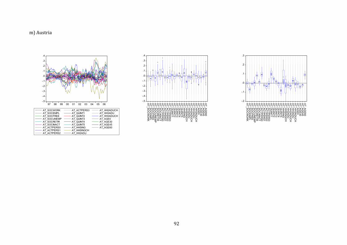
m) Austria

-.5

-.4

-.3

-.2

-.1

.0

.1

.2

.3

.4

97 98 99 00 01 02 03 04 05 06

AT_SOCWORKAT_SOCEMPLAT_SOCFREEAT_SOCUNEMPAT_SOCRETIRAT_SOCINACTAT_ACTPERS0AT_ACTPERS1AT_ACTPERS2

AT_ACTPERS3AT_QUINT1AT_QUINT2AT_QUINT3AT_QUINT4AT_QUINT5AT_HHSINGAT_HHSINGCHAT_HH2ADU

AT_HH2ADUCHAT_HH3ADUAT_HH3ADUCHAT_AGE0AT_AGE30AT_AGE45AT_AGE60

-.5

-.4

-.3

-.2

-.1

.0

.1

.2

.3

.4

AT_S

OC

WO

RK

AT_S

OC

EMPL

AT_S

OC

FRE

EA

T_SO

CU

NE

MP

AT_S

OC

RE

TIRA

T_SO

CIN

AC

TA

T_AC

TPE

RS0

AT_A

CTP

ER

S1A

T_AC

TPE

RS2

AT_A

CTP

ER

S3A

T_QU

INT1

AT_Q

UIN

T2A

T_QU

INT3

AT_Q

UIN

T4A

T_QU

INT5

AT_H

HSIN

GA

T_HH

SING

CH

AT_H

H2A

DU

AT_H

H2A

DU

CH

AT_H

H3A

DU

AT_H

H3A

DU

CH

AT_A

GE0

AT_A

GE30

AT_A

GE45

AT_A

GE60

-.2

-.1

.0

.1

.2

.3

AT_S

OC

WO

RK

AT_S

OC

EMPL

AT_S

OC

FRE

EA

T_SO

CU

NE

MP

AT_S

OC

RE

TIRA

T_SO

CIN

AC

TA

T_AC

TPE

RS0

AT_A

CTP

ER

S1A

T_AC

TPE

RS2

AT_A

CTP

ER

S3A

T_QU

INT1

AT_Q

UIN

T2A

T_QU

INT3

AT_Q

UIN

T4A

T_QU

INT5

AT_H

HSIN

GA

T_HH

SING

CH

AT_H

H2A

DU

AT_H

H2A

DU

CH

AT_H

H3A

DU

AT_H

H3A

DU

CH

AT_A

GE0

AT_A

GE30

AT_A

GE45

AT_A

GE60

92

n) Portugal

-.8

-.6

-.4

-.2

.0

.2

.4

.6

97 98 99 00 01 02 03 04 05 06

PT_SOCWORKPT_SOCEMPLPT_SOCFREEPT_SOCUNEMPPT_SOCRETIRPT_SOCINACTPT_ACTPERS0PT_ACTPERS1PT_ACTPERS2

PT_ACTPERS3PT_QUINT1PT_QUINT2PT_QUINT3PT_QUINT4PT_QUINT5PT_HHSINGPT_HHSINGCHPT_HH2ADU

PT_HH2ADUCHPT_HH3ADUPT_HH3ADUCHPT_AGE0PT_AGE30PT_AGE45PT_AGE60

-.8

-.6

-.4

-.2

.0

.2

.4

.6

PT_S

OC

WO

RK

PT_S

OC

EMPL

PT_S

OC

FRE

EP

T_SO

CU

NE

MP

PT_S

OC

RE

TIRP

T_SO

CIN

AC

TP

T_AC

TPE

RS0

PT_A

CTP

ER

S1P

T_AC

TPE

RS2

PT_A

CTP

ER

S3P

T_QU

INT1

PT_Q

UIN

T2P

T_QU

INT3

PT_Q

UIN

T4P

T_QU

INT5

PT_H

HSIN

GP

T_HH

SING

CH

PT_H

H2A

DU

PT_H

H2A

DU

CH

PT_H

H3A

DU

PT_H

H3A

DU

CH

PT_A

GE0

PT_A

GE30

PT_A

GE45

PT_A

GE60

-.8

-.6

-.4

-.2

.0

.2

.4

.6

PT_S

OC

WO

RK

PT_S

OC

EMPL

PT_S

OC

FRE

EP

T_SO

CU

NE

MP

PT_S

OC

RE

TIRP

T_SO

CIN

AC

TP

T_AC

TPE

RS0

PT_A

CTP

ER

S1P

T_AC

TPE

RS2

PT_A

CTP

ER

S3P

T_QU

INT1

PT_Q

UIN

T2P

T_QU

INT3

PT_Q

UIN

T4P

T_QU

INT5

PT_H

HSIN

GP

T_HH

SING

CH

PT_H

H2A

DU

PT_H

H2A

DU

CH

PT_H

H3A

DU

PT_H

H3A

DU

CH

PT_A

GE0

PT_A

GE30

PT_A

GE45

PT_A

GE60

93

o) Finland

-.8

-.6

-.4

-.2

.0

.2

.4

.6

97 98 99 00 01 02 03 04 05 06

FI_SOCWORKFI_SOCEMPLFI_SOCFREEFI_SOCUNEMPFI_SOCRETIRFI_SOCINACTFI_ACTPERS0FI_ACTPERS1FI_ACTPERS2

FI_ACTPERS3FI_QUINT1FI_QUINT2FI_QUINT3FI_QUINT4FI_QUINT5FI_HHSINGFI_HHSINGCHFI_HH2ADU

FI_HH2ADUCHFI_HH3ADUFI_HH3ADUCHFI_AGE0FI_AGE30FI_AGE45FI_AGE60

-.8

-.6

-.4

-.2

.0

.2

.4

.6

FI_SO

CW

OR

KFI_S

OC

EMPL

FI_SO

CFR

EE

FI_SO

CU

NE

MP

FI_SO

CR

ETIR

FI_SO

CIN

AC

TFI_A

CTP

ER

S0

FI_AC

TPE

RS

1FI_A

CTP

ER

S2

FI_AC

TPE

RS

3FI_Q

UIN

T1FI_Q

UIN

T2FI_Q

UIN

T3FI_Q

UIN

T4FI_Q

UIN

T5FI_H

HS

ING

FI_HH

SIN

GC

HFI_H

H2A

DU

FI_HH

2AD

UC

HFI_H

H3A

DU

FI_HH

3AD

UC

HFI_A

GE

0FI_A

GE

30FI_A

GE

45FI_A

GE

60 -.3

-.2

-.1

.0

.1

.2

.3

.4

FI_SO

CW

OR

KFI_S

OC

EM

PLFI_S

OC

FRE

EFI_S

OC

UN

EM

PFI_S

OC

RETIR

FI_SO

CIN

AC

TFI_A

CTP

ERS0

FI_AC

TPER

S1FI_A

CTP

ERS2

FI_AC

TPER

S3FI_Q

UIN

T1FI_Q

UIN

T2FI_Q

UIN

T3FI_Q

UIN

T4FI_Q

UIN

T5FI_H

HS

ING

FI_HH

SIN

GC

HFI_H

H2A

DU

FI_HH

2AD

UC

HFI_H

H3A

DU

FI_HH

3AD

UC

HFI_A

GE

0FI_A

GE

30FI_A

GE

45FI_A

GE

60

94

p) Sweden

-.8

-.6

-.4

-.2

.0

.2

.4

.6

.8

97 98 99 00 01 02 03 04 05 06

SE_SOCWORKSE_SOCEMPLSE_SOCFREESE_SOCUNEMPSE_SOCRETIRSE_SOCINACTSE_ACTPERS0SE_ACTPERS1SE_ACTPERS2

SE_ACTPERS3SE_QUINT1SE_QUINT2SE_QUINT3SE_QUINT4SE_QUINT5SE_HHSINGSE_HHSINGCHSE_HH2ADU

SE_HH2ADUCHSE_HH3ADUSE_HH3ADUCHSE_AGE0SE_AGE30SE_AGE45SE_AGE60

-.8

-.6

-.4

-.2

.0

.2

.4

.6

.8

SE

_SO

CW

OR

KS

E_S

OC

EM

PL

SE

_SO

CFR

EE

SE

_SO

CU

NE

MP

SE

_SO

CR

ETIR

SE

_SO

CIN

AC

TS

E_A

CTP

ER

S0

SE

_AC

TPE

RS

1S

E_A

CTP

ER

S2

SE

_AC

TPE

RS

3S

E_Q

UIN

T1S

E_Q

UIN

T2S

E_Q

UIN

T3S

E_Q

UIN

T4S

E_Q

UIN

T5S

E_H

HS

ING

SE

_HH

SIN

GC

HS

E_H

H2A

DU

SE

_HH

2AD

UC

HS

E_H

H3A

DU

SE

_HH

3AD

UC

HS

E_A

GE

0S

E_A

GE

30S

E_A

GE

45S

E_A

GE

60 -.3

-.2

-.1

.0

.1

.2

.3

.4

SE_SO

CW

OR

KS

E_SOC

EM

PL

SE_SO

CFR

EES

E_SOC

UN

EMP

SE_SO

CR

ETIR

SE_SO

CIN

AC

TS

E_ACTP

ER

S0

SE_AC

TPE

RS

1S

E_ACTP

ER

S2

SE_AC

TPE

RS

3S

E_QU

INT1

SE_Q

UIN

T2S

E_QU

INT3

SE_Q

UIN

T4S

E_QU

INT5

SE_H

HS

ING

SE_H

HS

ING

CH

SE_H

H2A

DU

SE_H

H2A

DU

CH

SE_H

H3A

DU

SE_H

H3A

DU

CH

SE_AG

E0

SE_AG

E30

SE_AG

E45

SE_AG

E60

95

96

q) United Kingdom

-1.0

-0.5

0.0

0.5

1.0

97 98 99 00 01 02 03 04 05 06

UK_SOCWORKUK_SOCEMPLUK_SOCFREEUK_SOCUNEMPUK_SOCRETIRUK_SOCINACTUK_ACTPERS0UK_ACTPERS1UK_ACTPERS2

UK_ACTPERS3UK_QUINT1UK_QUINT2UK_QUINT3UK_QUINT4UK_QUINT5UK_HHSINGUK_HHSINGCHUK_HH2ADU

UK_HH2ADUCHUK_HH3ADUUK_HH3ADUCHUK_AGE0UK_AGE30UK_AGE45UK_AGE60

-1.0

-0.5

0.0

0.5

1.0

UK

_SO

CW

OR

KU

K_S

OC

EM

PLU

K_S

OC

FRE

EU

K_S

OC

UN

EM

PU

K_S

OC

RE

TIRU

K_S

OC

INAC

TU

K_A

CTP

ER

S0U

K_A

CTP

ER

S1U

K_A

CTP

ER

S2U

K_A

CTP

ER

S3U

K_Q

UIN

T1U

K_Q

UIN

T2U

K_Q

UIN

T3U

K_Q

UIN

T4U

K_Q

UIN

T5U

K_H

HSIN

GU

K_H

HSIN

GC

HU

K_H

H2A

DU

UK

_HH

2AD

UC

HU

K_H

H3A

DU

UK

_HH

3AD

UC

HU

K_A

GE0

UK

_AG

E30U

K_A

GE45

UK

_AG

E60 -.4

-.3

-.2

-.1

.0

.1

.2

.3

UK

_SO

CW

OR

KU

K_S

OC

EM

PL

UK

_SO

CFR

EE

UK

_SO

CU

NE

MP

UK

_SO

CR

ETIR

UK

_SO

CIN

AC

TU

K_A

CTP

ER

S0

UK

_AC

TPE

RS

1U

K_A

CTP

ER

S2

UK

_AC

TPE

RS

3U

K_Q

UIN

T1U

K_Q

UIN

T2U

K_Q

UIN

T3U

K_Q

UIN

T4U

K_Q

UIN

T5U

K_H

HS

ING

UK

_HH

SIN

GC

HU

K_H

H2A

DU

UK

_HH

2AD

UC

HU

K_H

H3A

DU

UK

_HH

3AD

UC

HU

K_A

GE

0U

K_A

GE

30U

K_A

GE

45U

K_A

GE

60

97

Looking at the Box-Whisker-Plots for the overall period, we observe the following: 1. In the majority of countries, low-income households, households with no active persons in the labour market, unemployed, single households and pensioners are the population groups most strongly affected by higher inflation, though the difference is, on average, rather small. In fact, if the box of the Box-Whisker-Plot is taken as a strong and simple significance bound, inflation for these types of households is not different from average inflation.10 In contrast, higher income households, households with several active persons on the labour market and younger persons are less affected by inflation. 2. This observation holds for the majority of countries in the Euro area but is simi-larly true for the non-Euro area countries as well. However, there are a few no-table exceptions, with Portugal being the most prominent one. Looking at the Box-Whisker-Plots for the period 2001/2002, the picture is as follows: 1. Overall, the effect on inflation dispersion appears to be more pronounced than for the full sample. Again, the low-income, non-working groups or households with retired persons are the most strongly affected households. This conclusion holds for all large EMU countries but also for a number of smaller countries (Germany, France, Italy, Netherlands, Luxembourg, Austria, Belgium). Interest-ingly, a similar pattern is observable for Denmark, Sweden and Finland, which points to non-changeover related reasons. 2. There are a few countries where the opposite is true: Spain, Ireland and Greece among the EMU member countries and the United Kingdom. Here, high-income households seem to be affected more by price changes relative to the median household. The main reason can be probably found in the development of ahouse nd real-estate prices, affecting types of households differently. 3. There is a special effect in Germany (2003/2004) which mainly reflects the change in the financing of the ’health reform‘ in Germany so that individuals suddenly have to pay a 10€ fee each quarter at the doctor's. In practice, this is booked as a dramatic increase in household expenditures in the category ‘health’ but hits different types of household quite differently. Since it is a one-time effect, we do not discuss this aspect in detail.

10 The box of the Box-Whisker plot shows the range of the interquartile range. This is a robust measure of variance and by definition contains only the middle-50-percent of the distribution mass. A regular signifi-cance test would include at least 95 percent. Therefore the criterion is much stronger than typical signifi-cance tests. If the hypothesis has to be rejected by the graphical test it clearly will be rejected with any other test.

4. Regarding the question if these effects can be attributed to changeover-related inflation, we are not able to confirm that those kind of households with higher shares of their expenditures in those categories which are hit by cash change-over-related price increases, show higher inflation rates in general. In contrast, in most countries it is just the opposite: those in low-income categories suffered more. This raises doubts in the hypothesis that the temporarily higher inflation after 2002 might be due to the cash changeover effect.

98

ary around a mean of zero)? The investigation of differences might overshadow the fact, that even if differences in in-flation rates are small, accumulated differences over several years might be non-negligable. How large are the accumulated differences?Question (1) is tested using two approaches. One of them is the approach developed by Hobijn and Franses (2000) which has recently also been applied by Busetti, Forni, Harvey, and Venditti (2006) to test for

b.4) Econometric evaluation of price effects for different households As we have discussed so far, there are several categories of goods whose prices were es-pecially hard hit by the Euro changeover. Furthermore, differences in the consumption basket across socio-economic groups are detectable. Overall, the picture is in line with the results from previous studies. Besides that there are ’general‘ trends at work, shift-ing the weights of certain categories in the aggregate basket which can either dampen or aggravate certain changeover-related price shifts. In the following, we analyse a number of issues in more detail applying rigorous econo-metric techniques. e cl sW as ify the questions as follows: 1. Can we identify certain inflation clusters or clubs across the socio-economic groups, i.e., can we identify ’groups‘ of households with ’similar‘ inflation rate behaviour? Is there any sign that the variance of household-group specific infla-tion across countries – measured as a difference to the aggregate inflation rate – shows signs of systematic behaviour (put differently: are certain types of households more prone to higher variation of inflation). 2. Is there a common driving force behind all individual inflation rates in each country? 3. If the answer to question 2 is "yes", how is the behaviour of the cross-section variance in the panel of household-specific inflation rates which is not ex-plained by the common component (the main driving force for the variation in the panel)? 4. How do the idiosyncratic components (i.e., the part of the household-specific in-flation rate which is not covered by the common component) behave in the long-run. To put it another way: Are there any household-specific inflation rates which diverge from the common component in the longer-run and show no sign of mean-reversion (formally: are the idiosyncratic components station-

clubs in the national inflation rates in the Euro area. This is used to test if there are cer-tain clusters within each country. Furthermore, we employ as a second approach panel

99

regression techniques to test for similarities across countries. Questions (2) to (4) are tested using the PANIC approach (‘Panel Analysis of Nonstation-arity in Idiosyncratic and Common components’) that has been recently developed by Bai and Ng (2001, 2004) to decompose non-stationary panels and panel unit-root tests (here, for reasons of simplicity, we rely on those tests where a test statistic for the model without a constant is easily available). A more detailed description and technical outline of the applied econometric methods can be found in the appendix. We turn directly to the results which we sort along the questions raised above. Question 1: Can we identify "clusters" in household-specific inflation rates as well as in the variance of inflation? In a first step, we analyze whether we can find a systematic pattern in household-specific inflation rates, i.e., can we identify ’groups‘ of households with ’similar‘ inflation rate behaviour within each country. n I le b.1 the results are shown which can be summarized as follows: 1. The number of clusters is high; there are many "clusters" that consist of only one time series. This finding is in line with the hypothesis that systematic clus-

Tab tering does not seem to play any role here. 2. The groups of households which were previously identified as groups affected by higher-than-average inflation are not systematically clustered. To visualize this result, we use red colour for the ’typical‘ low-income household groups (unemployed, inactive persons, no active person in the labour market, single households, old-age, first quintile). As one can easily observe, there are no sys-tematic patterns (with a few exceptions).

100

Table b.1 Results of clustering procedures

Cluster Country 1 2 3 4 5 6 7 8 9 10 11 12 EU15 SOCWORK SOCFREE ACTPERS3 QUINT1 QUINT2

SOCINACT QUINT4 QUINT5 HH2ADU HH3ADU MIC1999 ACTPERS1 QUINT3 AGE45_59

MAC2000 HHSINGCH HH2ADUCH ACTPERS2 AGE0_29 AGE30_44

ACTPERS0 HHSING AGE60_ Euro area MIC1999 SOCWORK QUINT3 HHSING AGE45_59

SOCFREE SOCINACT ACTPERS1 ACTPERS2 QUINT2 QUINT4 QUINT5 HH3ADU HH3ADUCH

MAC2000 HHSINGCH AGE0_29 ACTPERS0 ACTPERS3 HH2ADU

QUINT1 HH2ADUCH AGE30_44 AGE60_ Belgium MAC2000 ACTPERS0 QUINT2 HHSING HH2ADU AGE60_

ACTPERS2 ACTPERS3 QUINT5 HHSINGCH AGE30_44

SOCUNEMP ACTPERS1 QUINT1 QUINT3 AGE45_59 MIC1999 SOCEMPL HH3ADU AGE0_29

SOCFREE SOCINACT HH2ADUCH HH3ADUCH SOCWORK QUIN RETIR T4 SOC Denmark QUINT2 QUINT4 HH2ADUCH HH3ADU AGE45_59

SOCFREE QUINT1 HHSINGCH AGE0_29 SOCEMPL SOCUNEMP ACTPERS3 AGE30_44

SOCWORK QUINT3 QUINT5 HHSING MIC1999 ACTPERS2 HH2ADU MAC2000 SOCINACT AGE60_ ACTPERS0 ACTPERS1 HH3ADUCH SOCRETIR

101

ADU

Germany SOCFREE ACTPERS3 QUINT4 HH2ADUCH AGE45_59 SOCUNEMP SOCINACT ACTPERS1 HHSING

MIC1999 ACTPERS2 HH2ADU SOCWORK QUINT3 AGE30_44

QUINT1 QUINT2 AGE0_29 QUINT5 HH3ADUCH AGE60_ MAC2000 HHSINGCH ACTPERS0 H3

Ireland SOCFREE ACTPERS2 QUINT3 AGE30_44 SOCUNEMP SOCINACT HH2ADU AGE60_

SOCEMPL ACTPERS3 HHSINGCH HH2ADUCH QUINT1 QUINT2 QUINT5 HH3ADU

MAC2000 SOCRETIR HHSING MIC1999 SOCWORK QUINT4 ACTPERS1 AGE0_29 AGE45_59 HH3ADUCH ACTPERS0

Greece SOCWORK SOCEMPL ACTPERS2 AGE0_29 SOCFREE HH3ADU AGE45_59

SOCUNEMP QUINT2 QUINT5 SOCRETIR HHSINGCH HH2ADU

QUINT1 HH2ADUCH AGE30_44 SOCINACT ACTPERS0 QUINT3 QUINT4 HHSING AGE60_ MIC1999 ACTPERS1 HH3ADUCH ACTPERS3 MAC2000 Spain MAC2000 SOCUNEMP HH3ADUCH AGE0_29

QUINT4 QUINT5 HH2ADUCH AGE30_44 SOCINACT HHSING HH2ADU AGE60_

SOCEMPL SOCRETIR ACTPERS1 SOCFREE QUINT2 QUINT3

SOCWORK HH3ADU AGE45_59 ACTPERS2 QUINT1 ACTPERS3 ACTPERS0 MIC1999 HHSINGCH France SOCUNEMP QUINT1 QUINT2 QUINT3 HH3ADU AGE60_

SOCINACT HHSING HH2ADUCH AGE0_29 AGE30_44 MIC1999 QUINT4 AGE45_59

MAC2000 ACTPERS0 ACTPERS3 QUINT5 HHSINGCH SOCRETIR HH2ADU SOCEMPL SOCFREE SOCWORK HH3ADUCH ACTPERS1 ACTPERS2

102

PERS2

Italy ACTPERS0 QUINT5 HHSING HH2ADU AGE60_ SOCFREE HH3ADU AGE30_44 AGE45_59

MAC2000 ACTPERS3 QUINT1 SOCRETIR SOCINACT QUINT4

SOCUNEMP HH3ADUCH AGE0_29 QUINT2 HHSINGCH HH2ADUCH

MIC1999 ACTPERS1 QUINT3 SOCWORK ACTLuxemburg SOCWORK SOCFREE ACTPERS1 QUINT1 HH3ADUCH

MAC2000 QUINT2 QUINT3 QUINT4 HH2ADU ACTPERS2 ACTPERS3 HHSINGCH HH2ADUCH

SOCEMPL SOCUNEMP AGE0_29 HHSING HH3ADU MIC1999 AGE45_59 SOCRETIR SOCINACT QUINT5 AGE30_44 AGE60_ 0 ACTPERSNetherlands SOCRETIR ACTPERS0 HHSING

SOCFREE QUINT1 HH2ADU MIC1999 ACTPERS1 QUINT3

QUINT4 QUINT5 HHSINGCH SOCEMP HH2ADUCH AGE0_29

ACTPERS2 HH3ADU AGE30_44 AGE60_ QUINT2 SOCWORK AGE45_59 SOCINACT Austria MIC1999 SOCWORK SOCINACT QUINT1 QUINT4 HH3ADUCH

ACTPERS1 ACTPERS3 QUINT2 HH2ADUCH AGE0_29

ACTPERS2 QUINT5 HH2ADU AGE30_44 AGE45_59 SOCFREE SOCRETIR QUINT3 HH3ADU

MAC2000 SOCEMPL SOCUNEMP ACTPERS0 HHSING HHSINGCH AGE60_ Portugal SOCUNEMP ACTPERS1 QUINT2 HH2ADU

ACTPERS0 QUINT1 HHSING HHSINGCH QUINT5 HH2ADUCH HH3ADU HH3ADUCH

SOCEMPL ACTPERS2 ACTPERS3 SOCWORK SOCFREE QUINT4 AGE45_59 AGE60_ MAC2000 AGE0_29 MIC1999 QUINT3 SOCRETIR AGE30_44 SOCINACT

103

0

Finland QUINT1 QUINT3 HHSINGCH HH3ADU AGE45_59 SOCWORK SOCINACT HH2ADUCH HH3ADUCH

QUINT2 HHSING HH2ADU MIC1999 SOCUNEMP QUINT5

ACTPERS2 ACTPERS3 AGE30_44 SOCEMPL SOCFREE ACTPERS1 QUINT4 MAC2000 AGE0_29 SOCRETIR AGE60_ ACTPERSSweden ACTPERS0 ACTPERS1 QUINT2 QUINT3 HHSING HHSINGCH

MAC2000 SOCEMPL SOCINACT ACTPERS2 AGE30_44 ACTPERS3 QUINT5 HH2ADUCH AGE0_29

SOCWORK QUINT1 HH2ADU MIC1999 QUINT4 HH3ADU SOCFREE HH3ADUCH SOCUNEMP AGE60_ AGE45_59 SOCRETIR

United Kingdom SOCUNEMP ACTPERS1 HH3ADU AGE60_ SOCEMPL QUINT1 HH2ADU

MAC2000 ACTPERS2 QUINT2 ACTPERS3 QUINT3 AGE0_29

ACTPERS0 QUINT5 AGE45_59 SOCFREE SOCINACT HHSING

SOCWORK HH2ADUCH AGE30_44 SOCRETIR QUINT4 HHSINGCH MIC1999 HH3ADUCH MIC1999… Aggregate basket based on micro-data, MAC2000…HICP basket

In a second step, we run the following regression: we regress the difference of each household-specific inflation rate (i) to the respective HICP for a number of countries (j)

tjiY ,, on a constant

104

α and a number of Dummies 1−iD . The estimations were performed in a simple pooled regression, the constant and coefficients on the dummies are re-stricted to be the same across countries, we are therefore searching for similar effects across countries – using the efficiency gains from panel regression.11 The regression re-sults can be understood in the following way. Since the number of dummies is smaller than the number of household-specific rates, we implicitly normalize the results to that missing rate. This base rate here was chosen to be the criterion "inactive" (which is automatically done by the procedure used here and in fact is not relevant for the overall result). We therefore ask: are certain households on average significantly different with regard to their inflation rate they face – measured against a somewhat arbitrarily chosen base rate. Negative and significant coefficients indicate that the rates are significantly lower and vice versa.

11 We also checked for robustness by using a fixed-effect model with and without time dummies as well. The results are similar.

105

Table b.2 Panel regression results (level)

Identifier C oefficient

Implied average

deviation from HICP

(across all countries) actPers0 0 .0541*** 0.139 actPers1 -0.0131 0.071 actPers2 -0.0341** 0.050 actPers3 - 0.0389*** 0.046 age0_29 -0.0317** 0.053 age30_44 - 0.0321** 0.052 age45_59 -0.0166 0.068 age60_ 0 .0572*** 0.142 hh2Adu 0.00551 0.090 hh2AduCh - 0.0398*** 0.045 hh3Adu -0.00800 0.076 hh3AduCh -0.310*** -0.226 hhSing 0.0582*** 0.143 hhSingCh -0 * .0485** 0.036 quint1 -0.0180 0.066 quint2 -0.00632 0.078 quint3 -0.00151 0.083 quint4 - 0.00853 0.076 quint5 -0.0116 0.073 socEmp -0.490*** -0.406 socFree -0.0260* 0.058 socRetir -0.265*** -0.181 socUnemp - 0.377*** -0.293 socWork -0.0172 0.067 In general, this exercise confirms the findings of the previous analysis. First of all, sys-tematic differences are small (indeed very small). Some exceptions can be found within the employment status categories: here we find systematic differences across Europe of the size of about half a percentage point. However, this is by far the largest deviation – all other deviations – even if they are significant – are quite small. Furthermore, the analysis reveals the pattern described above: people falling in certain categories – across Europe – seem to face a slightly lower inflation rate than the chosen baseline rate over the investigation period. This is true for households with persons ac-tive on the labour market, households of a younger age, households with two or three adults and children but even for single households with children. In contrast, older age households, single households, households with no active persons face a somewhat higher inflation. To illustrate the size of the effect, we calculated the implied average de-viation of the respective group from the HICP as a benchmark over the ten years aver-age. As can be seen, the highest effects for the categories "no active persons" and "age

above 60" with an inflation rate which is across Europe on average of 0.14 percentage points higher. On the other side, people falling in the category "non-manual worker" faced a lower inflation rate – which indeed is remarkably low (0.4 percentage points on average). But also the "unemployed" in the categorical definition of the household-specific baskets

106

faced a lower inflation rate on average in Europe. In a second exercise, we also checked for systematic differences in the variance of infla-tion across Europe. We did the same regression exercise with the only difference that the dependent variable was calculated as the standard deviation of the respective differ-ence between the household-specific rate and the HICP. The question therefore is: do households face fluctuations of different order around the HICP? As a benchmark we re-fer to the category "unemployed". Table b.3 Panel regression results (S.D.)

Identifier C toefficien Implied S.D.actPers0 0.00387 0.186actPers1 -0.0436*** 0.138actPers2 -0.0587*** 0.123actPers3 -0.0636*** 0.118age0_29 -0.0367*** 0.145age30_44 -0.0547*** 0.127age45_59 -0.0567*** 0.125age60_ -0.0103*** 0.172hh2Adu -0.0342*** 0.148hh2AduCh -0.0628*** 0.119hh3Adu -0.0539*** 0.128hh3AduCh -0.0433*** 0.139hhSing 0.0166*** 0.199hhSingCh -0.0324*** 0.150quint1 -0.0343*** 0.148quint2 -0.0437*** 0.138quint3 -0.0468*** 0.135quint4 -0.0494*** 0.133quint5 -0.0260*** 0.156socEmp -0.00839** 0.174socFree -0.0517*** 0.130socInact -0.01 1***1 0.171socRetir 0.0251*** 0.207socUnemp 0.182socWork -0.0588*** 0.123 The answer is again yes and no. On the one hand almost all coefficients are significant which indicates that the differences in volatility are almost all significant. However when it comes to the volatility implied by these coefficients, the differences are of course visi-ble but probably not as large as some people might expect. There is a number of low volatility categories – these are the some further above described as being close to the "median" household, i.e. households with 2 adults and one child, households in the mid-

dle age, households with two or three active persons. On the other end of the spectrum, we see the retired, unemployed, older-age households which seem to face a somewhat higher volatility in the inflation rates. However the range is from 0.1 to 0.2 – which in it-self is not a very large number.

107

Question 2: Is there a common driving force behind household-specific inflation rates? Our results indicate that there is indeed one common driving force which explains, in all countries, between 97 to 99% of the variation in each panel when principal component analysis is applied to the changes in inflation rates (a typical procedure to avoid mis-specification due to non-stationarity issues). Table b.4 Variance proportion in the panel of changes in household-specific inflation, explained by the first two common factors.

Variance

proportion of…

Country 1s rt facto 2n ord factEU15 0.993 0.005Euro area 0.992 0.006Belgium 0.989 0.008Denmark 0.981 0.012Germany 0.985 0.008Ireland 0.981 0.016Greece 0.982 0.012Spain 0.985 0.010France 0.992 0.005Italy 0.983 0.014Luxemburg 0.996 0.003Netherlands 0.984 0.012Austria 0.991 0.005Portugal 0.977 0.017Finland 0.974 0.021Sweden 0.982 0.014United Kingdom 0.976 0.017 The result is impressive. It is in line with the observation that deviations from the aggre-gate consumer price changes are very small in most countries most of the time. How-ever, this finding also implies that there is little evidence for persistent and lasting de-viations from the common trend in inflation observable in the data. Question 3: How large is the cross-section variance in the panel of household-specific infla-tion rates, which is not driven by the common factor? Is there a change in the dispersion over time? Both questions can be answered applying the procedure by Bai and Ng (2004). The proce-dure is explained in more detail in the appendix. Briefly, we decompose the changes in the time series into the effect of the common component and the idiosyncratic components and accumulate the results to draw conclusions for the inflation rates.

Figure b.5 gives an impression of the standard deviations across households for each country at any time in the sample, measured by the idiosyncratic components from the Bai and Ng (2004) procedure. Figure b.5 is roughly comparable to Figure b.3; the main difference is that here the reference series for calculating the standard deviation is not the deviation of each individual inflation rate from the aggregate inflation but from the first principal component inherent in all inflation rates. Figure b.5 Cross-section S.D. of idiosyncratic components

.0

.1

.2

.3

.4

.5

.6

97 98 99 00 01 02 03 04 05 06

AT_SD

.0

.1

.2

.3

.4

.5

.6

97 98 99 00 01 02 03 04 05 06

BE_SD

.0

.1

.2

.3

.4

.5

.6

97 98 99 00 01 02 03 04 05 06

DK_SD

.0

.1

.5

.4

.3

.2

.6

108

97 98 99 00 01 02 03 04 05 06

ES_SD

.0

.1

.2

.3

.4

.5

.6

97 98 99 00 01 02 03 04 05 06

FI_SD

.0

.1

.2

.3

.4

.5

.6

97 98 99 00 01 02 03 04 05 06

FR_SD

.0

.1

.2

.3

.4

.5

.6

97 98 99 00 01 02 03 04 05 06

GR_SD

.0

.1

.5

.4

.3

.2

.6

97 98 99 00 01 02 03 04 05 06

IE_SD

.0

.1

.2

.3

.4

.5

.6

97 98 99 00 01 02 03 04 05 06

LU_SD

.0

.1

.2

.3

.4

.5

.6

97 98 99 00 01 02 03 04 05 06

PT_SD

.0

.1

.2

.3

.4

.5

.6

97 98 99 00 01 02 03 04 05 06

SE_SD

.0

.1

.2

.3

.4

.5

.6

97 98 99 00 01 02 03 04 05 06

UK_SD

.0

.1

.2

.3

.4

.5

.6

97 98 99 00 01 02 03 04 05 06

EU15_SD

.0

.1

.2

.3

.4

.5

.6

97 98 99 00 01 02 03 04 05 06

EA_SD

.0

.1

.2

.3

.4

.5

.6

97 98 99 00 01 02 03 04 05 06

DE_SD

.0

.1

.5

.4

.3

.2

.6

97 98 99 00 01 02 03 04 05 06

IT_SD

.0

.1

.2

.3

.4

.5

.6

97 98 99 00 01 02 03 04 05 06

NL_SD

As one can see, the picture is roughly similar: The standard deviation is low for most countries (maybe a bit higher than in the previous experiment). More notably, the in-crease in dispersion around 2001/2002 that is detectable for several countries can also

be found in Sweden and UK. The variance seems to be fairly stationary for most coun-tries – a fact we will test rigorously later.

109

Question 4: Are the idiosyncratic components stationary?In a next step, we proceed by testing the stationarity of the idiosyncratic components around a mean of zero using panel unit root tests (as explained in more detail in the ap-

pendix). The overall result points to strong evidence for stationarity around a mean of zero: This finding is in line with the hypothesis that deviations from the common component are non-systematic in the long run, mean-reverting and do not last forever. In most coun-tries, it seems to be indeed a largely non-systematic phenomenon which groups are hit by certain inflation shocks. The major exception is evidence for the United Kingdom where the house price and real-estate price boom of the past decade seems to have led to a long-lasting decoupling of certain household-specific inflation rates from the common trend. To some extent, such eatures are also present in Greece and Spain, though far less pronounced. f

110

Table b.5 Unit Root-Tests of idosyncratic components Test Levin, Lin & Chu Breitung AD her Ch ) F (Fis i-Square PP her Chi ) (Fis Square Country at. ue at. ue at. ue at. uSt p-val St p-val St p-val St p-val e EU15 -7.143 0.000 -2.061 0.020 100.998 0.000 83.055 0.000 Euro area -8.089 0.000 -3.764 0.000 121.534 0.000 115.280 0.000 Belgium -8.807 0.000 -6.842 0.000 164.685 0.000 234.952 0.000 Denmark -9.541 0.000 -4.746 0.000 167.249 0.000 160.211 0.000 Germany -8.676 0.000 -5.487 0.000 131.182 0.000 136.860 0.000 Ireland -7.900 0.000 -5.814 0.000 136.794 0.000 150.291 0.000 Greece -4.334 0.000 -0.045 0.482 70.630 0.029 68.877 0.040 Spain -5.360 0.000 -0.028 0.489 118.944 0.000 109.100 0.000 France -7.413 0.000 -3.249 0.001 113.195 0.000 127.968 0.000 Italy -9.271 0.000 -4.842 0.000 160.247 0.000 154.174 0.000 Luxemburg -6.053 0.000 -2.968 0.002 121.829 0.000 130.664 0.000 Netherlands -7.924 0.000 -4.589 0.000 123.260 0.000 126.775 0.000 Austria -7.957 0.000 -4.322 0.000 137.478 0.000 154.908 0.000 Portugal -7.935 0.000 -4.390 0.000 147.274 0.000 156.200 0.000 Finland -11.139 0.000 -5.969 0.000 195.640 0.000 196.530 0.000 Sweden -8.385 0.000 -2.615 0.005 130.584 0.000 157.158 0.000 United Kingdom 3.265 1.000 -3.232 0.001 14.302 1.000 18.157 1.000

111

age point in Spain. • For the third group (Netherlands, Finland, Sweden, UK, and mostly pronounced Ireland), the general tendency, that poor and elderly faced a higher inflation, holds similar to the first group, but the size of the effect is more pronounced. The effect is on average about twice as high as in the first group for most coun-tries. The effect is about three to four times as high for Ireland. The most obvi-ous explanation stems from the above-mentioned observation that in Ireland, this might be due to the strong cross-household dispersion especially in cate-gory "Housing, water, electricity, fuels".

Question 5: How large are the accumulated inflation differentials? Even if the differences between household-specific inflation rates are in general small and econometric procedures typically do reject the hypothesis that these differences are lasting, it might be interesting for policy makers however to see how large the accumu-lated differences over the last decade were. Even more interesting, such a calculation makes national differences possibly more pronounced and visible. We therefore accu-mulated the inflation differentials for different time horizons (1997–2006, 1999–2006, 2002–2006) with the idea to see if certain tendencies have been amplified or dampened after the cash changeover. To have a better interpretation of the data, the accumulated differences are re-scaled in such a way that they now reflect the percentage point differ-ences in price levels between the HICP and the respective price level for different household groups. First and foremost, looking at EU15 or Euro area data, the accumulated differentials are small. Over a 10 years horizon, the differences are far less than 1 percentage points (for the Euro area as a whole even less than 0.5 percentage points). Certain spikes point to these types of households which were already identified above as having been more prone to higher than average inflation – poor, single households without children, eld-erly. Other types of households faced somewhat lower inflation than the HICP indicated, single households with children (possibly due to means-tested assistance), households with more than one active person on the labour market, households with 2 adults and children for example. On average, the accumulated effect for Europe as a whole is quite moderate. The picture is different if we look at member state levels. We observe three groups of countries. • In the first group (Belgium, Denmark, Germany, Greece, France, Italy, Luxem-burg, Austria) the effects are small but somewhat higher than for the EU15 or the Euro area. In general, the tendencies explained above hold: poor and elderly people as well as single households were somewhat more prone to inflation in the last decade. In general, however, the effect is quite small. In some of these countries – Germany, e.g., – higher income households also faced a slightly higher inflation than the median household over the sample. • The second group (Spain, Portugal) consists of countries were middle- and higher income groups faced higher inflation over the sample. Here indeed, a (mild) cash changeover effect might be at work. The effect is in the range of 1–1.5 percentage points over the entire period for Portugal and below 1 percent-

112

Figure b.6Accumulaa) EU 15

ted differences to HICP (socio-economic groups)

b) Euro area -1

-0.8

-0.6

-0.4

-0.2

0

0.2

0.4

0.6

0.8

1

Sum 1997-2006

Sum 1999-2006

Sum 2002-2006

-1

-0.8

-0.6

-0.4

-0.2

0

0.2

0.4

0.6

0.8

1

Sum 1997-2006

Sum 1999-2006

Sum 2002-2006

113

c) Belgium

-5

-4

-3

-2

-1

0

1

2

3

4

5

Sum 1997-2006

Sum 1999-2006

Sum 2002-2006

d) Denmark

-5

-4

-3

-2

-1

0

1

2

3

4

5

Sum 1997-2006

Sum 1999-2006

Sum 2002-2006

114

e) Germany

f) Ireland -5

-4

-3

-2

-1

0

1

2

3

4

5

Sum 1997-2006

Sum 1999-2006

Sum 2002-2006

-5

-4

-3

-2

-1

0

1

2

3

4

5

Sum 1997-2006

Sum 1999-2006

Sum 2002-2006

115

g) Greece

h) Spain -5

-4

-3

-2

-1

0

1

2

3

4

5

Sum 1997-2006

Sum 1999-2006

Sum 2002-2006

-5

-4

-3

-2

-1

0

1

2

3

4

5

Sum 1997-2006

Sum 1999-2006

Sum 2002-2006

116

i) France

j) Italy -5

-4

-3

-2

-1

0

1

2

3

4

5

Sum 1997-2006

Sum 1999-2006

Sum 2002-2006

-5

-4

-3

-2

-1

0

1

2

3

4

5

Sum 1997-2006

Sum 1999-2006

Sum 2002-2006

117

k) Luxemburg

l) Netherlands -4

-3

-2

-1

0

1

2

3

4

5

Sum 1997-2006

Sum 1999-2006

Sum 2002-2006

-5

-5

-4

-3

-2

-1

0

1

2

3

4

5

Sum 1997-2006

Sum 1999-2006

Sum 2002-2006

118

m) Austria

n) Portugal -4

-3

-2

-1

0

1

2

3

4

5

Sum 1997-2006

Sum 1999-2006

Sum 2002-2006

-5

-5

-4

-3

-2

-1

0

1

2

3

4

5

Sum 1997-2006

Sum 1999-2006

Sum 2002-2006

119

o) Finland

p) Sweden -4

-3

-2

-1

0

1

2

3

4

5

Sum 1997-2006

Sum 1999-2006

Sum 2002-2006

-5

-5

-4

-3

-2

-1

0

1

2

3

4

5

Sum 1997-2006

Sum 1999-2006

Sum 2002-2006

q) United Kingdom

-5

-4

-3

-2

-1

0

1

2

3

4

5

Sum 1997-2006

Sum 1999-2006

Sum 2002-2006

b.5) Conclusion We can draw the following conclusions: 1. Household types differ in the weighting schemes as measured by their con-not sumption baskets. It is a priori clear whether these differences lead to a pronounced and lasting deviation of group-specific inflation rates from a ’rep-resentative‘ basket. 2. The empirical evidence reveals that the differences are the more pronounced he m r socio-economic characteristics from ’m iat o e different households are in theira ed n‘ household. A country’s median household is in almost all cases very close to either: • a household with 1 active person, • a household in the fourth quintile (60–80% in the income distribution), or • a household with 2 adults and no dependent children. 3. In the majority of countries, low-income households, households with no active persons in the labour market, unemployed, single households and pensioners are the groups most strongly affected by higher inflation, although the effect is, 120

on average, small. In contrast, higher income households, households with sev-eral active persons on the labour market and younger persons are less affected by inflation.

121

4. The euro changeover in 2002 is accompanied by an increase in inflation disper-sion. This increase, however, is neither very pronounced when compared to other episodes nor is it obvious that there is a clear causality to the changeover (Sweden and UK show an increase in dispersion of similar magnitude). 5. The results of the econometric tests so far do neither point to clustering nor to a lasting divergence (non-stationarity) of group-specific inflation rates from ei-ther the aggregate inflation rate (HICP) or the ’common component’. Further-more, the ’common component‘ (the first principal component) explains the overwhelming bulk of the variance in the panel of group-specific inflation rates in almost all countries. 6. The calculation of accumulated differences showed, that with the exception of some Nordic and Anglo-Saxon countries the differences are quite moderate over a 5 to 10 years horizon. Nevertheless, there is evidence that in the period under investigation the poor and the elderly faced a somewhat higher inflation. The evidence, however, is not limited to Euro area countries and the cash changeover event can therefore not be blamed to be responsible for that evi-dence. Food, energy and housing prices seem to be the main driver. In the “out-lier” countries Ireland and UK, the house-price-boom related inflation factors might be at the root of astonishingly high accumulated inflation differentials over the last decade. 7. Interestingly, countries with real-estate price booms (United Kingdom, Ireland, Spain) seem to deviate in some tests. This should be further investigated but is beyond the questions raised in this report.

122September: 32–42. Hagemann, Robert P. (1982): The Variability of Inflation Rates across Household Types, Journal of Money, Credit and Banking, 14, 494–510.

References Amble, Nathan and Stewart, Kenneth (1994): Experimental Price Index for Elderly Con-sumers, Monthly Labor Review, May: 11–16. Bai, Serena and Bai, Jushan (2001): A PANIC Attack on Unit Roots and Cointegration, Boston College Working Papers in Economics 519, Boston College Department of Economics. Bai, Serena and Bai, Jushan (2002): Determining the numbers of factors in approximate factor models, Econometrica, 2002, 70, 191–221. Bai, Serena and Bai, Jushan (2004): A PANIC Attack on Unit Roots and Cointegration, Econometrica, 2004, 72, 1127–1177. Breitung, Jörg (2000): The Local Power of Some Unit Root Tests for Panel Data,” in B. Baltagi, ed., Nonstationary Panels, Panel Cointegration, and Dynamic Panels, Vol. 15 of Advances in Econometrics, Amsterdam: JAI Press, pp. 161–178. Brewer, Mike, Goodman, Alissa and Leicester, Andrew (2006): Household Spending in Britain. What Can it Teach us about Poverty? Joseph Rowntree Foundation, York. Busetti, Fabio, Forni, Lorenzo, Harvey, Andrew and Venditti, Fabrizio (2006): Inflation convergence and divergence within the European Monetary Union, ECB Work-ing Paper Series 574, European Central Bank 2006. Chiru, Radu (2005a): Does Inflation Vary with Income? Statistics Canada, Analytical Pa-per No. 11-621-MIE2005-30. Chiru, Radu (2005b): Is Inflation Higher for Seniors? Statistics Canada, Analytical Paper No. 11-621-MIE2005-27. Choi, In (2001): Unit Root Tests for Panel Data, Journal of International Money and Fi-nance, 2001, 20, 249–272. Crawford, Ian and Smith, Zoë (2002): Distributional Aspects of Inflation, Institute for Fiscal Studies, Commentary 90, London. Del Giovane, Paolo and Sabbatini, Roberto (2006): Perceived and Measured Inflation Af-ter the Launch the Euro: The Gap in Italy, Giornale degli Economisti e Annali di Economia, 65, 2: 155–192. Dickey, David A. and Fuller, Wayne A. (1979): Distribution of the Estimators for Autore-gressive Time Series with a Unit Root, Journal of the American Statistical Asso-ciation, 74, 427–431. Döhring, Björn and Mordonu, Aurora (2007): What Drives Inflation Perceptions? Euro-pean Commission, Economic Papers No. 284, July. Garner, Thesia, Johnson, David and Kokoski, Mary (1996): An Experimental Consumer Price Index for the Poor, Monthly Labor Review,

Hobijn, Bart and Lagakos, David (2005): Inflation Inequality in the United States, Review

123

of Income and Wealth, 51, December: 581–606. Hobijn, Bart and Franses, Phillip Hans (2000): Asymptotically perfect and relative con-vergence of productivity, Journal of Applied Econometrics, 2000, 15: 59–81. Idson, Todd and Miller, Cynthia (1997): The Implications of Demographic-Specific Infla-tion Rates for Trends in Real Educational Wage Differentials, Journal of Business & Economic Statistics, 15, 4: 464–469. Kwiatkowski, Denis, Phillips, Peter C., Schmidt, Peter C.B. and Shin, Yongcheoul (1992): Testing the null hypothesis of stationarity against the alternative of a unit root, Journal of Econometrics, 1992, 54, 159–178. Levin, Andrew, Lin, Chien-Fu and Chu, Shia-Shang (2002): Unit root tests in panel data: Asymptotic and finite sample properties, Journal of Econometrics, 108, 1–24. Livada, Alexandra (1990): The Distribution of Household Inflation: The Greek Experi-ence, Bulletin of Economic Research, 43, 3: 175–196. Maddala, G. S. and Wu, Shaowen (1999): A Comparative Study of Unit Root Tests with Panel Data and A New Simple Test, Oxford Bulletin of Economics and Statistics, 61, 631–52. Magrabi, Frances M., Chung, Young Sook, Cha, Sanghee Sohn and Yang, Se-Jeong (1991): The Economics of Household Consumption, Praeger, New York. Michael, Robert T. (1979): Variation across Households in the Rate of Inflation, Journal of Money, Credit, and Banking, 11: 32–46. Noll, Heinz-Herbert (2007): Household Consumption, Household Incomes and Living Standards. A Review of Related Recent Research Activities, mimeo, GESIS-ZUMA, Mannheim. Noll, Heinz-Herbert and Weick, Stefan (2006): Strukturen des privaten Verbrauchs in Deutschland: Ungleichheiten und temporärer Wandel, in: Karl-Siegbert Rehberg (ed.) Soziale Ungleichheit, Kulturelle Unterschiede, Campus, Frankfurt am Main: 407–423. Noll, Heinz-Herbert and Weick, Stefan (2007): Einkommensarmut und Konsumarmut – unterschiedliche Perspektiven und Diagnosen, Informationsdienst Soziale Indi-katoren, 37, January: 1–6. Phillips, Peter C.B. and Perron, Pierre (1988): Testing for a Unit Root in Time Series Re-gression, Biometrika, 75, 335–346. Rippin, Franziska (2006): Gibt es gruppenspezifische Inflation? Eine Sensitivitätsanalyse mit Hilfe der Einkommens- und Verbrauchsstichprobe, Master-Thesis, Univer-sity of Erfurt.

124

Appendix

Box 1 Sensitivity Analysis: 1999 versus 2005 data vintage During the period, when the final report was prepared, Eurostat made a number of newly calculated household-specific consumption baskets available. The actual wave of data now refers to 2005. We therefore used the new wave of COICOP-based consump-tion baskets (the weights), to perform a sensitivity analysis on how this might affect the calculation of household-specific inflation rates. a) Comparison of weights of the data sets used in the interim report

and the newly published 2005 weights As a first exercise, we compared the weights used so far (see above) with the new weights based on the 2005 wave. So far, we used a hypothetical consumption basket which on the one hand follows the changes of the weights as measured for the aggregate consumer over time – therefore the weights for the aggregate or representative con-sumer follows the HICP chain index – and on the other hand kept the relative distance of the household-specific weights to the aggregate consumer constant at its 1999 position. The new data set gives now more detailed information for 2005, so we can evaluate the error. A first inspection of the new data, however shows, that the data are preliminary and far from being complete. We therefore decided to leave out all the categories with obvious problems – this was relevant for Italy, Euro area, EU 15, Sweden, Luxembourg and espe-cially for the age categories. We then computed the differences in weights.

125

Figure b.A.1 Euro area: Differences in weights between 1999 and 2005 (as a fraction of 1000)

Remind that the basket weights are measured as a fraction of 1000. That implies that the highest observable deviation in the basket structure is less than 50 per mille or 5 per cent in the basket. To save space we do not report all. Closer inspection reveals that in the majority of countries the deviations are even smaller than the reported ones, the ma-jor outliers with slightly higher differences are Ireland, Greece and Portugal. The differ-ences in large Euro area countries like Spain, France are small; Germany as the largest country in terms of GDP weight is somewhere in the middle range. To sum up, from the differences in weights, we would not expect to see large differences in inflation rates.

-200

-150

-100

-50

0

50

100

150

200

socW

ork

socE

mp

socF

ree

socU

nemp

socR

etir

socIn

act

actPers

0

actPers

1

actPers

2

actPers

3qu

int1qu

int2qu

int3qu

int4qu

int5

hhSing

hhSing

Ch

hh2A

du

hh2A

duCh

hh3A

du

hh3A

duCh

Food, and non-alcoholic beverages Alcoholic beverages and tobacco

Clothing and footwear Housing, water, electricity, gas and other fuels

Furnishings, household equipment and maintenance of house Health

Transport Communication

Recreation and culture Education

Hotels, cafes and restaurants Miscellaneous goods and services

b) Differences in inflation rates (distribution) As a second exercise, we did an experiment: For all household-specific characteristics, where we were able to get the weights, we calculated a household-specific index with constant 1999 weight and another one with constant 2005 weights. Both indices are somehow "imperfect" but by comparing both results, we can assess the scope for errors. This gives a total of 373 time series. We compute the differences in the results and graph the maximum, the minimum and the median (which should be less influenced by out-liers).

126

Figure b.A.2 Differences in household specific inflation rates (distributional aspects)

Measured by the median the deviation is positive in general. However, for the median of the difference in all possible household-specific inflation rates, the effect is very small (0.1 – 0.2, rate against previous year). The remarkable outliers in 2001 and 2005 (1.5 to 2 percent) are mainly due to differences on household-specific basket in Ireland and (to a far smaller extent) in Greece.

-1

-0.5

0

0.5

1

1.5

2

2.5

1997

m01

1997

m05

1997

m09

1998

m01

1998

m05

1998

m09

1999

m01

1999

m05

1999

m09

2000

m01

2000

m05

2000

m09

2001

m01

2001

m05

2001

m09

2002

m01

2002

m05

2002

m09

2003

m01

2003

m05

2003

m09

2004

m01

2004

m05

2004

m09

2005

m01

2005

m05

2005

m09

2006

m01

2006

m05

2006

m09

maxminmedian

c) Ireland and Greece: a somewhat deeper look The obvious question arises: what might be behind the shifts in baskets which explain the deviations in Ireland and Greece. First of all, let's have a look at the shifts in baskets. These changes are by far most pronounced in the case of Ireland.

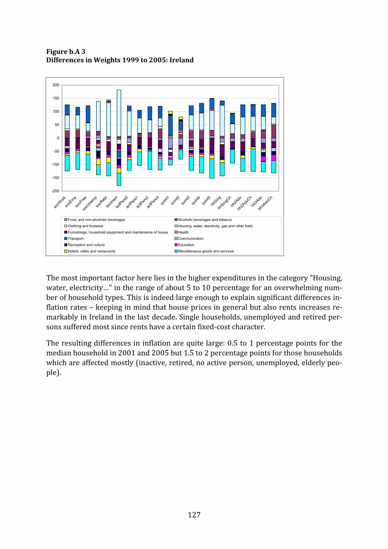
127

Figure b.A 3 Differences in Weights 1999 to 2005: Ireland

The most important factor here lies in the higher expenditures in the category "Housing, water, electricity…" in the range of about 5 to 10 percentage for an overwhelming num-ber of household types. This is indeed large enough to explain significant differences in-flation rates – keeping in mind that house prices in general but also rents increases re-markably in Ireland in the last decade. Single households, unemployed and retired per-

-200

-150

-100

-50

0

50

100

150

200

socW

ork

socE

mp

socF

ree

socU

nemp

socR

etir

socIn

act

actP

ers0

actP

ers1

actP

ers2

actP

ers3

quint

1qu

int2

quint

3qu

int4

quint

5

hhSing

hhSing

Ch

hh2A

du

hh2A

duCh

hh3A

du

hh3A

duCh

Food, and non-alcoholic beverages Alcoholic beverages and tobacco

Clothing and footwear Housing, water, electricity, gas and other fuels

Furnishings, household equipment and maintenance of house Health

Transport Communication

Recreation and culture Education

Hotels, cafes and restaurants Miscellaneous goods and services

sons suffered most since rents have a certain fixed-cost character. The resulting differences in inflation are quite large: 0.5 to 1 percentage points for the median household in 2001 and 2005 but 1.5 to 2 percentage points for those households which are affected mostly (inactive, retired, no active person, unemployed, elderly peo-ple).

128

Figure b.A 4 Differences in inflation rates as implied by different weights (1999/2005): Ireland

-1

-0.5

0

0.5

1

1.5

2

2.5

1997

m01

1997

m04

1997

m07

1997

m10

1998

m01

1998

m04

1998

m07

1998

m10

1999

m01

1999

m04

1999

m07

1999

m10

2000

m01

2000

m04

2000

m07

2000

m10

2001

m01

2001

m04

2001

m07

2001

m10

2002

m01

2002

m04

2002

m07

2002

m10

2003

m01

2003

m04

2003

m07

2003

m10

2004

m01

2004

m04

2004

m07

2004

m10

2005

m01

2005

m04

2005

m07

2005

m10

2006

m01

2006

m04

2006

m07

2006

m10

socWork socEmp socFree socUnemp socRetir socInact actPers0 actPers1 actPers2actPers3 quint1 quint2 quint3 quint4 quint5 hhSing hhSingCh hh2Aduhh2AduCh hh3Adu hh3AduCh age0_29 age30_44 age45_59 age60_

Next, we turn to the case of Greece. This is interesting as a country in catching-up but n Ireland. without a house price boom of the magnitude as iAgain, we inspect the changes in basket weights: Figure b.A 5 Differences in Weights 1999 to 2005: Greece

-200

-150

-100

-50

0

50

100

150

200

socW

ork

socE

mp

socF

ree

socU

nemp

socR

etir

socIn

act

actP

ers0

actP

ers1

actP

ers2

actP

ers3

quint

1qu

int2

quint

3qu

int4

quint

5

hhSing

hhSing

Ch

hh2A

du

hh2A

duCh

hh3A

du

hh3A

duCh

Food, and non-alcoholic beverages Alcoholic beverages and tobacco

Clothing and footwear Housing, water, electricity, gas and other fuels

Furnishings, household equipment and maintenance of house Health

Transport Communication

Recreation and culture Education

Hotels, cafes and restaurants Miscellaneous goods and services

129

In the case of Greece, we observe the shift towards "higher" COICOP categories, namely "Hotels, Cafes and Restaurants", "Recreation and Culture", "Health", "Clothing and "Footwear" across all household types. The reason behind that might be found in the remarkable increase of GDP per capita level as well as demand elasticities which might reflect national characteristics. Interestingly, expenditures for food decreases, as well as for communication (the latter one is a fact observable in most countries due to strong competition effects) but also expenditures for "Housing, Electricity, …". This is in stark contrast to the results in Ireland. The resulting differences in inflation rates are smaller than in Ireland. Figure b.A 6 Differences in inflation rates as implied by different weights (1999/2005): Greece

The distribution of households affected by somewhat higher inflation is less clear than in Ireland. Higher-income households, households with 3 active persons and unemployed – all face a higher inflation rate. The fact that households at the higher end of the income distribution are affected speaks clearly in favour of a "catching-up-cum-shift-towards-

-0.8

-0.6

-0.4

-0.2

0

0.2

0.4

0.6

0.8

1

1997

m01

1997

m04

1997

m07

1997

m10

1998

m01

1998

m04

1998

m07

1998

m10

1999

m01

1999

m04

1999

m07

1999

m10

2000

m01

2000

m04

2000

m07

2000

m10

2001

m01

2001

m04

2001

m07

2001

m10

2002

m01

2002

m04

2002

m07

2002

m10

2003

m01

2003

m04

2003

m07

2003

m10

2004

m01

2004

m04

2004

m07

2004

m10

2005

m01

2005

m04

2005

m07

2005

m10

2006

m01

2006

m04

2006

m07

2006

m10

socWork socEmp socFree socUnemp socRetir socInact actPers0 actPers1 actPers2actPers3 quint1 quint2 quint3 quint4 quint5 hhSing hhSingCh hh2Aduhh2AduCh hh3Adu hh3AduCh age0_29 age30_44 age45_59 age60_

more-sophisticated-good-categories" effect. As a result of this exercise – and keeping the incompleteness of the recent wave of data in mind – we decided to stick to the old data set for the final report.

130

Table b.A.1 Description of COICOP Categories

Category Description c beveragecp1 Food, and non-alcoholi s cp2 Alcoholic beverages and tobacco cp3 Clothing and footwear g, water, electricity, gas and other fuels s, household equipment and maintenance of house cp4 Housincp5 Furnishingcp6 Health cp7 Transport ation cp8 Communiccp9 Recreation and culture cp10 cp11 cp12 Education Hotels, cafes and restaurants Miscellaneous goods and services Table b.A.2 Country codes

Code Country AT Austria BE Belgium DE Germany ark DK DenmEA 5 Euro area untries ES Spain EU1 EU15 coFI FinlandFR France e GR GreecIE Ireland IT Italy rg ds LU LuxembunNL NetherlaPT SE UK Portugal Sweden United Kingdom

131

Table b.A.3 Identifiers for socio-economic characteristics

Consumption struc-re… tu

Descriptor (level 1)

Descriptor (level 2) by employment status SOC manual worker WORK non-manual worker EMPL self-employed FREE unemployed UNEMP retired RETIR inactive INACT by number of active ersons p ACT zero 0 one 1 two 2 three and more 3 by income quintile QUINT first 1 second 2 third 3 fourth 4 fifth 5 by household type HH single person SING single parent with dependent children SINGCH two adults 2ADU two adults with dependent children 2ADUCH three or more adults 3ADU three or more adults w. dep. hildren c 3ADUCH by age of reference erson p less than 30 0_29 30 to 44 years 30_44 45 to 59 years 45_59 60 years and older 60_

132

Table b.A.4 Availability of data according to household characteristics (using additive constraints to fill gaps)

CountryEuropean Union (15) Euro area Belgium Denmark Germany Ireland Greece Spain France Italy Luxemburg Netherlands Austria Portugal Finland Sweden United Kingdom

Consumption structure… Descriptor (level 1) Descriptor (level 2)by employment status SOC

manual worker WORKnon-manual worker EMPL X X X Xself-employed FREEunemployed UNEMP X X X Xretired RETIR X X Xinactive INACT

by number of active persons ACTzero 0one 1two 2three and more 3

by income quintile QUINTfirst 1second 2third 3fourth 4fifth 5

by household type HHsingle person SINGsingle parent with dependent children SINGCHtwo adults 2ADUtwo adults with dependent children 2ADUCHthree or more adults 3ADUthree or more adults w. dep. children 3ADUCH X

by age of reference personless than 30 0_2930 to 44 years 30_4445 to 59 years 45_5960 years and older 60_

133

Econometric methodologyIn the following, we outline the specific approaches used to test the behaviour of the time series econometrically.

The clustering approach of Hobijn and Franses (2000) The New Growth Theory allows for the possibility, that countries may not converge to the same level of per capita GDP, productivity or prices but instead sub-groups may form convergence clubs. Hobijn and Franses (2000) propose an algorithm for the identi-fication of convergence clubs based on multivariate stationarity tests. The procedure has recently been applied to regional EMU inflation rates (Busetti et al., 2006). Applying the algorithm using a version of stationarity test which does not allow for an intercept is equivalent to identifying clusters around the same mean (Busetti et al., 2006, p. 15). The procedure has the nice feature that it is independent of the ordering of the series. It is however, not invariant to the number of series in that sense that including additional se-ries may change the composition of clusters. The clustering algorithm (Hobijn and Franses, 2000, Busetti et al., 2006) is applied to a panel of all possible bivariate differentials in ULC growth rates and can be described as follows:12 1. Denote ik as a set of indices of variables in cluster *, nii ≤ , where *nn ≤ de-notes the number of clusters. Define *P as a significance level for the inclusion in the clu . Proc{ nk =

of a series eed with the following steps. e sster 2. Initializ } ,...,1, niii == o that each country/ variable is a cluster. 3. For all *, n

*ji ≤ , such that ji < perform a test whether ji kk ∪ form a cluster ac-cording to the criterion of a multivariate stationarity test on the contrast (here: by means of a multivariate version of the Kwiatkowski et al. (1992) test) and let

jiP , the resulting p-value of the test. Decide: If *, PP ji > for all ji , then go to the end of the procedure. 4. Replace cluster i by ji kk ∪ and drop jk where k ji , i, j correspond to the most likely cluster (maximum p-value of the previous step); replace the number of clusters by 1* −n and go one step back. 5. The resulting n∗ clusters are labelled “convergence clubs” (convergence to a common mean)) 6. The procedure proceeds in testing for relative convergence (convergence to a stationary distance) by applying the same procedure with different p-values. 12 We did not experiment with bandwidth for the multivariate KPSS test as in the paper by Hobijn and Franses (2000) but used the proposed value instead.

The PANIC approach of Bai and Ng (2004) Bai and Ng (2004) suggest a very useful approach to test for panel unit roots in the pres-ence of stationary or nonstationary common components, known as PANIC – Panel Analysis of Nonstationarity in the Idiosyncratic and Common components. The PANIC approach allows both idiosyncratic and common components to be integrated of order one, which makes it very flexible in testing panel unit roots. Since we investigate growth rates of prices, we assume a model with an intercept but without linear trend and fol-lowing the notation of Bai and Ng (2004) our model is:

FcX ++= 'λ ittiiit e

where itX are Ni ,...,1= observed household-specific inflation rates, tF is an unobserved vector of common factors and ite are unit specific idiosyncratic components. Both tF and ite are allowed to be I(1) and for this reason the model has to be estimated in differ-ences, where itit Xx Δ= , tt Ff Δ= , and itit ez Δ= , so we estimate the model: z+ ittit fx =

using the method of principal components. However, we standardize the first differ-ences before estimating in order to avoid possible distortions by volatile series in calcu-lating principal components, see Bai and Ng (2001). In particular, we divide di enced tim ries by their empirical cross-sectional standard deviations. Estimated mmon fact and idiosyncratic components are then obtained via cumulating for and .

'λ ffere se coors Tt ,...,2=,...,1 Ni =

∑=

=t

sisit ze 2 ˆˆ

∑=t

sit fF ˆˆ=s 2where iiitit fxz ˆˆˆ 'λ−= are estimated residuals. Bai and Ng (2004) show that estimated fac-tors and idiosyncratic components are consistent, in particular )1(ˆ 2/12/1

pitit oeTeT += −− and )1(ˆ 2/12/1ptt oHFTFT += −− , where

H is a full rank matrix. This rate of convergence is fast enough to leave the asymptotic distribution of the ADF-test unchanged, if applied to estimated series tF and ite . So we can apply the univariate ADF-test as well as pooled unit root tests to estimated factors and idiosyncratic components respectively. Another important issue is determining the number of factors in PANIC framework. Bai and Ng (2002) suggest some information criteria. But accordingly to Bai and Ng (2002) our sample size is too small to work with the suggested criteria. Therefore we calculated fractions of total variation in the differenced data. In all cases we found one dominating factor and therefore restricted the number of common factors to one.

134The unit root tests It is well known in the literature, that panel unit tests in a lot of cases have more power than individual tests. The panel unit root tests were performed using EViews 5.1 and the

respective standard settings with regard to lag length (BIC) and bandwidth selection

135

(Newey-West using Bartlett kernel) were taken. More specifically, we applied: • Tests based on a common unit root process: here the methods of Levin et al. (2002) and Breitung (2000) were considered. • Tests based on individual unit roots: here an augmented Dickey and Fuller (1979) test and the Phillips and Perron (1988) test in panel versions as pro-posed by Maddala and Wu (1999) and Choi (2001) were considered.

mechanisms, evidence turns out to be generally mixed. We begin our analysis by examining the dynamics in perceived and actual inflation over the period from 1996 to 2007. Perceived inflation is measured by the EU balance statistics; for actual inflation, we refer to the Harmonised Index of Consumer Prices (HICP) taken from Eurostat. For reasons of comparison, we use Sweden and the United Kingdom as control group. We find that the balance statistics of inflation perceptions tracks the dynamics of HICP inflation remarkably well for the period from 1996 to 2001; in statistical terms, the distance of the mean of both series displays a stationary relationship. However, there is a measurable break in this relationship at the time of the introduction of the euro. In all EMU member countries, perceived inflation dramatically jumps upwards, implying a shift in levels in the distance between inflation perceptions and HICP inflation rates. While a temporary gap between actual and perceived inflation is not unusual (for instance, similar changes in the distance between both inflation measures can be observed for the United Kingdom in 2000), the magnitude and persistence of the increase in perceived inflation are remarkable. Interestingly, while measures of actual and perceived inflation have converged again in Germany, Italy and the Netherlands, there is a persistent gap between both measures in France, Belgium, Greece and Finland. 137

c) The phenomenon of perceived inflation

Summary A core issue in the discussion about possible effects of the euro changeover on prices is the emergence of a sizable gap between official inflation rates as reported by statistical offices and inflation perceptions of consumers. The behaviour of perceived inflation during the euro cash changeover has been already well documented. Several explanations to rationalise the developments in inflation perceptions are presented; these explanations include: • the degree of macroeconomic (il)literacy influences the perception, • price movements of frequently bought products (which have been somewhat higher around the cash changeover) gain a higher attention, • there is an asymmetry in the perception of price increases relative to price decreases, • expected price movements influence actual perception, • complicated conversion rates might influence perceptions, • style and tone of media coverage are important channels of price perceptions (agenda setting). For all these explanations, some supportive evidence has been presented in the literature. Empirical studies typically use micro-level price and survey data; other studies present results from experimental designs. Overall, however, the relative importance of the various potential channels is unknown; for some of the proposed

We also explore whether differences in inflation perceptions are associated with differences in household-specific inflation rates. We find indeed evidence that “jumps” in perceptions are partly explained by differences in individual inflation experience. This finding holds for various types of households (divided by income group, income source and age). The effect has not only the expected sign; the results also show that the jump is considerably lower when the household-specific inflation rate is considered. This result t ivis remarkable since, as noted above, the quan itat e difference in inflation rates is small. Next, we investigate potential explanations for the observed jump in perceptions. In particular, we test the impact of explanatory variables proposed in the literature on inflation perceptions in Europe. Our baseline regression explains current inflation perceptions with its own lagged value, the level of inflation expectations, HICP inflation and a dummy variable for the euro cash changeover. As inflation perceptions may have been blurred by inflation expectations, we control for this effect (using again data from the balance statistics). To test for the impact of current inflation, we employ both the HICP index as well as an out-of-pocket index (FROOP)13. In line with the literature, we find that both the lag of perceptions and current inflation expectations have a significantly positive effect on inflation perceptions. In addition, actual inflation turns out to be a robust determinant of perceptions, except for Italy. A more notable result is that the persistence of inflation perceptions has increased dramatically in almost all countries after 2002. Before the introduction of euro notes and coins, the persistence coefficients ranged from about 0.4 to about 0.8. After the euro cash changeover, the degree of persistence ranges from about 0.6 to 0.7 for Ireland and Austria up to estimates of about 1.0 for Germany, Italy and the Netherlands. This result implies that unexplained shocks to perception are highly persistent. Moreover, the explanatory power of HICP inflation decreases dramatically. Furthermore, there is evidence that in some countries the influence of expectations on perceptions has increased. That is, inflation perceptions by consumers appear to be increasingly affected by their own inflation expectations, while putting less weight on official price statistics. However, the results are not robust across countries; for the Netherlands and Austria, we observe that

138

expectations have become less important. To explore the relevance of media reporting for the dynamics in inflation perceptions, we perform a case study analysis for Germany on the role of media coverage for public inflation perceptions. We employ two measures of incoming news on inflation. First, we apply simple count variables that capture how often a specific terminology is mentioned in the media. The count measures are on the one hand obtained by searching through a standard online database of media articles, LexisNexis. Second, we use data from Medientenor, a research institute that analyses media articles (TV and press) and provides careful codification. From this source, we have obtained media data covering statements dealing with inflation which are at least five lines long (in case of printed media) and last at least five seconds (for television broadcasts). The coding is based on the standards of the media content analysis. We are provided with the overall number of eports in that given period and the amount of reports dealing with rising or falling r

13 See: http://epp.eurostat.ec.europa.eu/cache/ITY_OFFPUB/KS-SF-09-015/EN/KS-SF-09-015-EN.PDF

inflation. Interestingly, we find that media reporting intensity and tone have indeed a significant impact on inflation perceptions. There is clear empirical evidence that the “teuro” debate in the media has driven inflation perceptions in Germany. In addition, news on prices materialise in inflation perceptions in an asymmetric manner, with news n having on avon rising inflatio erage much larger effects. Considering the economic magnitude of various determinants of inflation perceptions, media news outperform actual inflation numbers, especially in the second half of the sample. Examining the impact of media news according to various socioeconomic characteristics provides no conclusive evidence. In sum, we find empirical support for explanations of the gap between actual and perceived inflation, based on expected price movements, media coverage and the asymmetry of the reaction to price increases. In contrast, there is no evidence that macroeconomic illiteracy or the impact of frequently bought products have affected inflation perceptions.

139

c.0) Introduction Part c) sheds light on the phenomenon of perceived inflation. It touches upon results presented in parts a) and to a lesser extent b). It comprises a literature review which is presented in section c.1). The developments of realised inflation and inflation perception are depicted and analyzed on an aggregate level in section c.2). To explore the reasons for the developments presented in section c.2), an econometric analysis is offered in section c.3). The analysis consists mainly of three parts. First, a panel study as well as individual country regressions (c.3.i) are presented to investigate determinants put forward in the recent literature to be key drivers of inflation perceptions. In the next section we will explore the connection between household-specific inflation rates (section b) and inflation perception in more detail (section c.3.ii). Third, a case study (c.3.iii) for Germany is executed which specifically analyses the role media plays in driving and shifting inflation perceptions. c.1) Survey of the literature on perceived inflation A central aspect in the discussion about possible effects of the euro changeover is the occurrence of the wedge between inflation and inflation perceptions of the consumers in the aftermath of the introduction of the new currency. While both series exhibit a strong and stable correlation in all countries before the euro introduction, a clear mismatch between both series emerges after the introduction of the euro mainly driven by an explosive rise in inflation perceptions – often manifested as a level jump. The behaviour of perceived inflation during the euro cash changeover has been well documented by Ehrmann (2006) as well as Döhring and Mordonu (2007). Although perceived inflation is not a well-defined concept, there are several reasons why one should care about any distortions in the perceptions of the public. Stix (2006) raises several arguments of them we highlight two. First, increased price perceptions might have real effects if the overestimation of price increases leads to an underestimation of the purchasing power of households and yields into a reduction in spending (see for instance Hofman et al., 2006). Moreover, inflation perceptions might feed into inflation expectations. Deteriorations in inflation expectation in turn would have consequences for wage claims and investment decisions. Evidence for a possible spillover from inflation perceptions to inflation expectations is provided by Fluch and Stix (2005). This view was recently supported by the survey of the Bank of England and the study by Blanchflower and Kelly (2008), who conclude that price expectations are influenced by past inflation experience. Acknowledging the relevance of inflation perceptions and observing a structural break in the formerly tight relationship between perceived and actual inflation, the strong rise in inflation perception and its persistence for some euro countries gave rise to an p

140

extensive search and debate on the driving forces of inflation erception. Several explanations to rationalise the developments in inflation perceptions are presented in Fluch and Stix (2005), Eife and Coombs (2007) as well as Del Giovane and Sabbatini (2006). The following explanations are presented:

141

perceptions. A further explanation – which is closely linked to the above-mentioned theoretical arguments – is stated by Traut-Mattausch et al. (2004). The authors present

• the degree of macroeconomic (il)literacy influences the perception, • price movements of frequently bought products (somewhat higher around the cash changeover) gain a higher attention, • there is an asymmetry in the perception of price increases relative to price decreases, • expected price movements influence actual perception, • complicated conversion rates might influence perceptions, tone of media coverage • style and are important channels (agenda setting). With respect to macroeconomic literacy several studies provide evidence that people have difficulties assessing macroeconomic figures. Del Giovanne et al. (2008) conclude using survey data on consumers for Italy that a low degree of literacy on inflation and inaccurate price recall are significant in explaining extreme perceptions. Related to the literacy of macroeconomic figures is the ability to recall past prices. Cestari et al. (2007) demonstrate the limited capabilities of Italian consumers in recalling past price movements and argue that this might lead to distortions in inflation perceptions. Overall they referred to price far before the euro introduction using them still as a benchmark. Very recently, Blanchflower and Kelly (2008) in a study of report a widespread “illiteracy” and “innumeracy” among the general public. Two explanations for a “perception miracle” are embedded in the study by Brachinger (2006) and underlie the construction of his index of “perceived inflation” on behalf of the German Statistical Office. They are based on the works by Kahneman and Tversky (1979) and Burgoyne at al. (1999). The first argue that goods that are bought more frequently receive a greater attention than price changes in less frequent bought product groups. The latter argue that especially price increases are received more powerfully. The empirical evidence is mixed: based on micro data, Stix (2006) shows that people which are confronted with price increase on frequently purchased goods, who hold expectations on price increases and who still convert all prices into their old currency, have significantly higher inflation perceptions. Above that he argues the increase in perception due to the euro cash changeover is more persistent if people meet these characteristics (expectations of future price increases and conversion into old currency). A recently published study using results from experiments in Berlin (Jungermann et al., 2007) supports at least the theoretical arguments underlying the index constructed by Brachinger (2006). There is evidence that people perceive price increases and decreases er l adifferently and that frequently bought goods receive a high evel of ttention. On the other hand, Aucremanne et al. (2007) find little empirical evidence that per-ceptions are especially driven a frequent bought goods and services. Further evidence against the "Brachinger hypothesis" is provided by Döhring and Mordonu (2007). In their study they show that the newly created out-of-the-pocket expenditure HICP index does not perform any better as the all-items HICP index in explaining inflation

142

and push away consumer expectations from the best possible conjecture. All the channels mentioned above are likely to be conditional on socioeconomic characteristics. Socioeconomic characteristics affect the consumption basket, the degree of macroeconomic literacy, individual inflation expectations and thereby move inflation perceptions and their accuracy. For instance low income households might face a higher proportion of "out-of-pocket" expenditures due to their consumption baskets, therefore these households are more prone to effects via price increases in certain retail sectors (food, transportation…). As the results from section b) showed, low income households were to some extent more prone to price increases in a majority of countries during the cash changeover. There are furthermore several studies that argue that there is substantial difference in assessing inflation perceptions between socioeconomic groups – which go clearly beyond the effects attributable to differences in consumption baskets. See for instance Bryan and Venkatu (2001) who show a clear gap in figures of guessed actual inflation for the US. Palmqvist and Strömberg (2004) prove that similar patterns

experimental evidence that links high inflation perceptions to the existence of a priori expectations of price increases before the cash changeover. Following their line of argumentation people selectively update only the share of information that complements their own expectations. Thus, if they expect prices to rise, they will most likely focus on and react to upward price movements. This argumentation finds support in the micro level study for Austria by Stix (2006) and – to some extent – by the results of Döhring and Mordonu (2007). A further explanation is directly linked to the euro introduction itself explains the cross country differences in the dynamics of perceptions by the different conversion rates. While the earlier arguments had some type of behavior in mind which is sometimes regarded as not in line with classical "rational expectation" approaches, the upcoming proposition assumes rational agents in the traditional sense but imputes that they have difficulties in information acquisition and processing. Agents might have problems with the different conversion rate and furthermore information provided might have a certain slant. Ehrmann (2006) argues that conversion rates matter for the reaction in perceived inflation. He observes that countries with least complicated conversion rates had lower inflation rates than countries which conversion rates were larger than 100. Finally, Kooremann et al. (2004) observe an increase in donations. This effect can be related to the phenomenon of "money illusion". Dziuda and Mastrobuoni (2006) find that the longer people stick to converting the euro prices into their old currency the more likely it is that they will overestimate current inflation. The obvious explanation for this phenomenon is that they neglect price increases that would have had happen if they had stick to their old currency. In addition to all mentioned effects, the style and tone of media reporting might induce distortionary effects. Del Giovanne et al. (2007) highlight, that media reporting might a huge proportion of the observable jump in perceptions. Lamla and Rupprecht (2008) analyse the impact of media reporting on consumers’ inflation expectations. They find that media reporting deteriorated the gap between professional expectations and inflation expectations of consumers during the cash changeover period 2002. This effect is likely to be driven by a media bias. In order to gain attention and increase their returns media agencies concentrate on certain events negative events, e.g., high inflation

143

U.K. as countries within the EMU that have not adopted the euro. The following patterns can be observed. This balance statistics track the dynamics of HICP inflation remarkably well in the period from 1996–2001 – the distance of the mean

exist for Sweden. In particular they find a u-shaped relationship between inflation perception and age as well as income. People up to midst of their lifetime improve their inflation expectation which deteriorates when they become elderly. They show that a similar pattern emerges not only for inflation perceptions but also for inflation expectations. Aucremanne et al. (2007) find no significant difference in the response to the cash changeover between different groups. However, they did not possess the data necessary to test this hypothesis in a detail. Moreover, both Stix (2006) and Dziuda and Mastrobuoni (2006) argue that household income, education level or age are factors determining changeover-induced inflation perceptions. Malgarini (2007) enriches this discussion by offering insights on the relationship between personal characteristics and the overestimation of inflation. He shows that in line with the aforementioned studies socioeconomic characteristics matter for the degree of overestimation of inflation figures. He notes that the degree of overestimation is lower the higher the level of education is. Furthermore, he shows that more optimistic respondents are prone to a lower degree of overestimation. Blanchflower and Kelly (2008) report very high "non-response" rates to inflation perceptions in surveys among the least educated, females, poorest and younger individuals. Furthermore, groups with "biased" perceptions form "biased" expectations as well. As Blinder and Krueger (2004) – in a survey for the US – show, people receive the bulk of information from media usage (TV mainly, with a large distance followed by newspapers), but do not actively search for information on economic issues. People with higher income as well as higher education are in general better informed. Furthermore, ideology plays a large role in the formation of public beliefs. This finding was recently reinforced in a survey by the University of Michigan (Curtin, 2007). Therefore the different usage structure of media by different household types might play an important role in explaining differences in perceptions. Information processing capacities – which are possibly not independent from educational status – are stressed as a further source of differing perceptions in the literature, see Sims (2003). With respect to inflation expectations, Inoue et al. (2006) provide evidence that the response of consumers’ expectations on news on inflation depend on the level of education. Bryan and Palmqvist (2005) test the near rationality of inflation expectations between countries using micro-level data. Summing up, the literature suggests that higher educated and high income individuals are less prone to deviations from HICP figures. c.2) Developments of perceived and actual inflation In this section we provide a descriptive overview with respect to the relationship between perceived and actual inflation in the Euro area. Upcoming figures depict the dynamics of perceived and actual inflation over one decade. Perceived inflation is measured by the EU balance statistics and for actual inflation we refer to the Harmonised Index of Consumer Prices (HICP) as taken from Eurostat. We include all data available. Therefore, Luxembourg and Malta have been excluded due to data restrictions. For reasons of comparison we consider additionally Sweden and the

144

of both series show a stationary relationship. However, for all countries of the first cohort, a mismatch between observed and perceived inflation starting at the time of the euro introduction can be observed. In all euro countries perceived inflation dramatically moves upwards and there is a level shift in the distance between perception and HICP. Consequently the monetary union average (EU-12) reveals a similar pattern.14 While a gap between HICP and perceived inflation as such is not a extraordinary event as can be seen both for countries that have adopted the euro and those that stayed out of the monetary union, see for instance the U.K. in the year 2000. The high increase which can be measured for all euro countries in the aftermath of the euro introduction and especially the persistence of the level of perceived inflation observable for several countries are substantial. Convergence between both measures can be observed in Germany, Italy and the Netherlands but persistence in the gap can be monitored in France, Belgium, Greece and Finland. For an excellent overview see also Ehrmann (2006) as well as Döhring and Mordonu (2007). Using statistical methods, Döhring and Mordonu (2007) find a substantial (and statistically significant) break in the co-movement of both series after the euro introduction. Similarly Lein and Maag (2008) observe that there is a substantial heterogeneity between countries in that by how much actual inflation and perceived inflation are correlated. They also note that the precision of the assessment of inflation figures – i.e. the correlation between both figures – deteriorates if one considers the post euro phase. Looking at the comparison group, there is no substantial mismatch observable between both series. Thus, the majority of the increase in perception can be attributed to direct or indirect effects of the introduction of the euro. Notably, both Sweden and the U.K. show a rise in perceptions although not adopting the new currency. However, this may be evidence that some other issues besides the introduction of the new currency contributed to a rise in perceptions. Some of them we already touched upon in part a). Those are for instance shocks to oil and gas prices but also a bad harvest that has affected food prices. They might likely have driven the perceptions of all European countries. For a robustness analysis we also transform the qualitative data into quantitative inflation figures. The perceived inflation rates are calculated using the method suggested by Carlson and Parkin (1975). This approach has lately been also applied by Forsells and Kenny (2005) as well as Lein and Maag (2008). All authors rely on a normal distribution to infer the absolute inflation numbers.15 The resulting figures which are not presented here exhibit a very high correlation with the original balance statistics (.95) and the qualitative conclusions are equivalent to the original figures. 14 For Italy the sharp increase seems to kick in with some delay. 15 Although the quantification of the qualitative data has been criticized it has been applied by various institutions as for instance the Bundesbank.

Figure c.1 Inflation and perceptions of countries that adopted the euro

−50

0

50

Per

ceiv

ed In

flatio

n

0

2

4

6

HIC

P

1996m1

1998m1

2000m1

2002m1

2004m1

2006m1

2008m1

Time

2002HICPPerceived Inflation

AT

0

20

40

60P

erce

ived

Infla

tion

0

2

4

6

HIC

P

1996m1

1998m1

2000m1

2002m1

2004m1

2006m1

2008m1

Time

2002HICPPerceived Inflation

BE

145

10

20

30

40

50

60

Per

ceiv

ed In

flatio

n

0

2

4

6

HIC

P

1996m1

1998m1

2000m1

2002m1

2004m1

2006m1

2008m1

Time

2002HICPPerceived Inflation

CY

0

20

40

60

80

Per

ceiv

ed In

flatio

n

0

2

4

6

HIC

P

1996m1

1998m1

2000m1

2002m1

2004m1

2006m1

2008m1

Time

2002HICPPerceived Inflation

DE

146

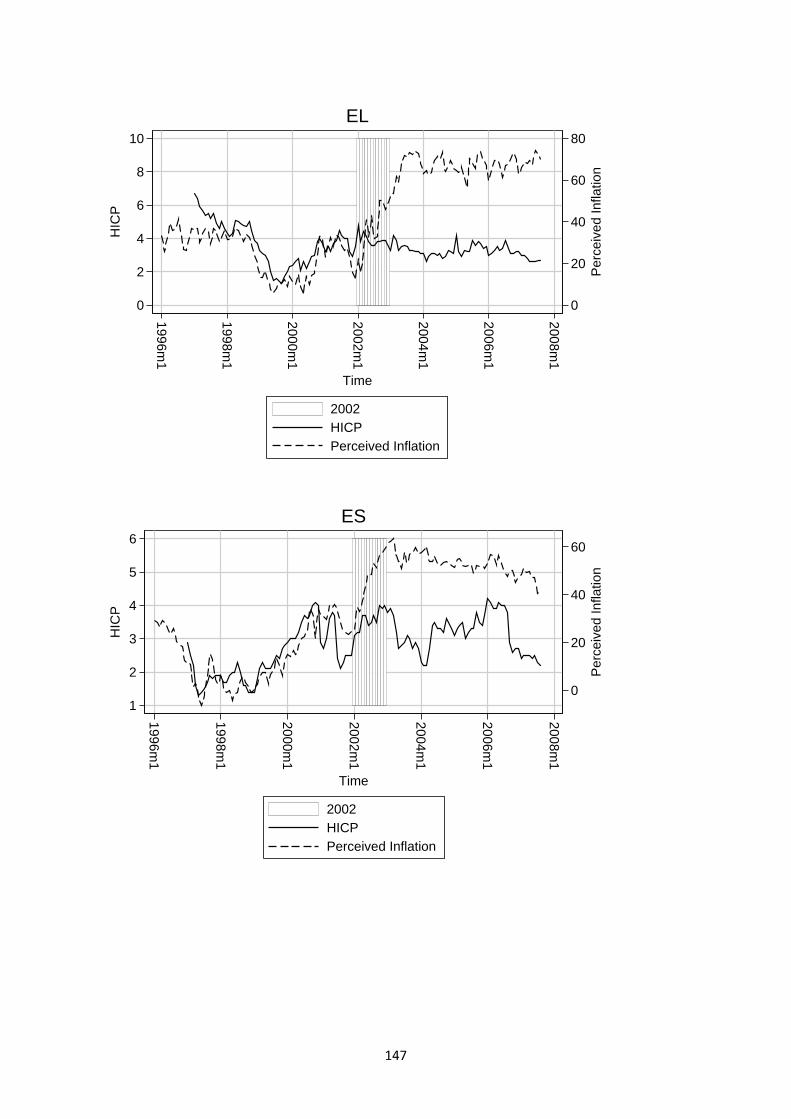
0

20

40

60

80

Per

ceiv

ed In

flatio

n

0

2

4

6

8

10

HIC

P

1996m1

1998m1

2000m1

2002m1

2004m1

2006m1

2008m1

Time

2002HICPPerceived Inflation

EL

0

20

40

60

Per

ceiv

ed In

flatio

n

1

2

3

4

5

6

HIC

P

1996m1

1998m1

2000m1

2002m1

2004m1

2006m1

2008m1

Time

2002HICPPerceived Inflation

ES

147

−60

−40

−20

0

Per

ceiv

ed In

flatio

n

0

2

4

6

HIC

P

1996m1

1998m1

2000m1

2002m1

2004m1

2006m1

2008m1

Time

2002HICPPerceived Inflation

FI

−20

0

20

40

60

Per

ceiv

ed In

flatio

n

0

2

4

6

HIC

P

1996m1

1998m1

2000m1

2002m1

2004m1

2006m1

2008m1

Time

2002HICPPerceived Inflation

FR

148

0

20

40

60

80

Per

ceiv

ed In

flatio

n

0

2

4

6

HIC

P

1996m1

1998m1

2000m1

2002m1

2004m1

2006m1

2008m1

Time

2002HICPPerceived Inflation

IE

0

20

40

60

80

Per

ceiv

ed In

flatio

n

1

2

3

4

5

6

HIC

P

1996m1

1998m1

2000m1

2002m1

2004m1

2006m1

2008m1

Time

2002HICPPerceived Inflation

IT

149

0

20

40

60

80

Per

ceiv

ed In

flatio

n

1

2

3

4

5

6

HIC

P

1996m1

1998m1

2000m1

2002m1

2004m1

2006m1

2008m1

Time

2002HICPPerceived Inflation

NL

0

20

40

60

Per

ceiv

ed In

flatio

n

0

2

4

6

8

10

HIC

P

1996m1

1998m1

2000m1

2002m1

2004m1

2006m1

2008m1

Time

2002HICPPerceived Inflation

SI

150

0

20

40

60

Per

ceiv

ed In

flatio

n

1

2

3

4

5

6

HIC

P

1996m1

1998m1

2000m1

2002m1

2004m1

2006m1

2008m1

Time

2002HICPPerceived Inflation

EA

151

Figure c.2 Inflation and perception, comparison group, non euro adopting countries

−40

−30

−20

−10

Per

ceiv

ed In

flatio

n

0

2

4

6

HIC

P

1996m1

1998m1

2000m1

2002m1

2004m1

2006m1

2008m1

Time

2002HICPPerceived Inflation

SE

−20

−10

0

10

20P

erce

ived

Infla

tion

0

2

4

6

HIC

P

1996m1

1998m1

2000m1

2002m1

2004m1

2006m1

2008m1

Time

2002HICPPerceived Inflation

UK

152

153

c.3) Econometric analysis In this section we are going to investigate somewhat deeper the reasons for perception jumps. In a first section, we are going to extend the approach by Döhring and Mordonu (2007) by looking at factors driving expectations (section c.3.i.). In contrast to Döhring and Mordonu (2007), here the focus is on panel as well as national level. In the next section we will explore the connection between household-specific inflation rates (section b) and inflation perception in more detail (section c.3.ii). This is done in a panel framework for all Euro area countries. Furthermore, we use a case study for Germany to discuss the relationship between media reporting and inflation perception jumps. Due to limited data availability in this field, the latter issue is investigated for German data only, where the project team had access to a quite unique and rich data set on media reports (tone and volume, see section c.3.iii). c.3.1) Factors driving the perception jumps: national and panel evidence This section tests the impact of explanatory variables proposed in the literature over- view on inflation perceptions. Our starting regression rests on the proposed testing setup by Döhring and Mordonu (2007). We estimate the current perception with its own lag value, inflation expectations, HICP inflation and a dummy variable controlling for the euro cash changeover. As inflation perceptions may have been blurred by inflation expectations we employ inflation expectations. For both series, we rely on the balance statistics data. Following Forsells and Kenny (2004), we use a six month lag of expectations. Notably a 12 month lag produces similar results. However, people might have a quite short-run memory. To test for the impact of current inflation we employ both the HICP index as well as an out of pocket index (FROOP). The latter index should reflect that perceptions could be more affected by prices of frequently purchased items. The dummy variable is constructed according to Döhring and Mordonu (2007). It has the value of zero until 2002 and the value of one afterwards. We use monthly observations from 1998 to 2007. The results of the initial regressions are presented in Tables c.1 and c.2 as well as in igures c.3 and c.4. F

Table c.1 Inflation perception drivers (HICP)

Full Sample

E n re ... stimatio sults for Variable Belgium Germany Ireland Greece Spain France Italy Netherlands Austria Finland All Euro L.perception 0.830*** 0.953*** 0.804*** 0.870*** 0.840*** 0.863*** 0.902*** 0.934*** 0.793*** 0.654*** 0.913*** L6.expectation 0.004 0.089*** -0.123*** -0.060 0.021 0.081** 0.059* 0.009 0.001 -0.005 0.013 Hicp 2.007*** 1.836*** 2.423*** 1.519*** 2.140*** 2.388*** 2.203 1.680*** 3.928*** 1.845*** 1.416*** Changeoverdummydoehring 2.007*** 1.836*** 2.423*** 1.519*** 2.140*** 2.388*** 2.203 1.680*** 3.928*** 1.845*** 1.416*** Constant 0.516 -3.639*** 2.288* -0.589 -2.704** -2.908*** -3.547 -2.862*** -6.056*** -7.998*** -1.828***Observations 122 122 122 122 122 122 122 122 122 122 1220 <2002 L.perception 0.662*** 0.819*** 0.810*** 0.710*** 0.678*** 0.806*** 0.882*** 0.421*** 0.442*** 0.628*** 0.834*** L6.expectation 0.175 -0.044 -0.084 -0.098* 0.198** 0.068 0.036 0.319** 0.266*** -0.146*** -0.012 Hicp 4.295*** 4.684*** 2.459*** 3.247*** 3.723*** 4.813*** 2.209 3.636*** 8.406*** 3.555*** 2.428*** Constant -1.960 -0.146 0.937 -1.572 -5.351*** -5.875*** -2.778 -5.627** -18.107*** -9.782*** -2.471***Observations 54 54 54 54 54 54 54 54 54 54 540 >2002 L.perception 0.853*** 0.981*** 0.629*** 0.878*** 0.833*** 0.684*** 0.930*** 0.955*** 0.742*** 0.539*** 0.935*** L6.expectation -0.006 0.098*** -0.289*** -0.018 -0.006 0.013 0.082* 0.025 -0.061 0.060*** 0.042*** Hicp 0.370 1.989* 2.891*** 0.924 1.329** -0.392 2.169 2.184* 1.028 1.737*** 1.300*** Constant 6.943** -4.445 14.324*** 5.593 4.693 15.276*** -1.580 -3.280*** 9.089** -4.936*** -0.725 Observations 68 68 68 68 68 68 68 68 68 68 680 *** p<0.01, ** p<0.05, * p<0.1

154

155

Table c.2 Inflation perception drivers (FROOP)

Full Sample E n re .. stimatio sults for .Variable Belgium Germany Ireland Greece Spain France Italy Netherlands Austria Finland All Euro L.perception 0.839*** 0.951*** 0.853*** 0.902*** 0.817*** 0.891*** 0.898*** 0.949*** 0.808*** 0.642*** 0.921*** L6.expectation -0.014 0.093*** -0.053 -0.049 0.034 0.076* 0.061* 0.027 0.063 0.013 0.024*** Froop 1.991*** 1.762*** 1.562*** 1.195** 1.425*** 1.359*** 1.259 1.276*** 2.109*** 1.470*** 0.970*** Changeoverdummydoehring 4.019*** 1.031 2.579*** 5.335*** 4.594*** 4.206*** 2.964** 2.091** 6.819*** 4.313*** 2.313*** Constant 0.143 -4.592*** -0.211 -1.605 -1.043 -2.829*** -1.359 -2.988*** -5.413*** -8.077*** -1.866***Observations 126 126 126 126 126 126 126 126 126 126 1405 <2002 L.perception 0.720*** 0.825*** 0.861*** 0.940*** 0.646*** 0.816*** 0.942*** 0.547*** 0.540*** 0.583*** 0.839*** L6.expectation 0.070 -0.048 -0.043 -0.101* 0.189* 0.078 0.025 0.367** 0.292*** -0.091** -0.002 Froop 4.121*** 3.428*** 2.044*** 1.334** 2.528*** 2.992*** -0.038 2.023*** 4.597*** 2.717*** 2.098*** Constant -2.505 -0.459 -2.844 -1.234 -2.541* -6.394*** 0.979 -6.049** -14.918*** -10.215*** -3.051***Observations 54 54 54 54 54 54 54 54 54 54 547 >2002 L.perception 0.874*** 0.984*** 0.650*** 0.893*** 0.818*** 0.856*** 0.916*** 0.971*** 0.850*** 0.569*** 0.932*** L6.expectation -0.012 0.104*** -0.246*** -0.020 0.006 0.061 0.079** 0.041 0.036 0.073*** 0.050*** Froop 1.094** 1.854*** 1.841*** 0.839 1.150*** 0.498 1.498 1.647** 1.056 1.202*** 0.808*** Constant 4.501 -5.297*** 14.879*** 4.891 5.136* 5.194 0.238 -2.731** 2.901 -4.712*** -0.089 Observations 72 72 72 72 72 72 72 72 72 72 858 *** p<0.01, ** p<0.05, * p<0.1

Figure c.3 nse of inflation perceptions after one S.D. shock (HICP) Impulse respoa) before 2002

b) after 2002

156

Figure c.4 nse of inflation perceptions after one S.D. shock (FROOP) Impulse respoa) before 2002

b) after 2002

157

158

Overall, our results are in line with the literature. Table c.1 contains the basic specification with HICP for all countries estimated individually and as a panel. In the upper part of the table, we present the results for a model with the changeover dummy – which captures the perception jump as a break in the constant of the model. The middle and lower part of the table contain results for period before and after 2002 – to control if certain slope coefficients change. In general, the own lag of perceptions (descriptor = l.perception) is highly significant in almost all cases and shows that the perception are strongly correlated over time. The range of the coefficient varies from 0.4 to 0.8 in the basic model with HICP and from 0.6 to close to one in the model with FROOP. Moreover, expectations (descriptor = l6.expectation) affect perceptions significantly in a number of cases. However this effect seems to differ across countries and – more importantly – across time. In addition inflation (descriptor = hicp) is a robust determinant of perceptions in almost all cases except Italy if we consider the full sample. There are some remarkable features in the regression results: first of all, the persistence of perception increased dramatically in almost all countries after 2002 compared to the pre-2002 values. Before 2002, the persistence coefficients ranged from 0.4 to 0.8 roughly. The degree of persistence after 2002 now ranges from 0.6 and 0.7 (Ireland and Austria) to the estimates of Germany, Italy and Netherlands with coefficient estimates around 1. This implies, that unexplained perception shocks are very persistent – even close to be of infinite impact.16 Secondly, the explanatory power of HICP decreases dramatically. The perceptions are now somehow anchored to HICP figures in Germany, Ireland, Spain and Finland – but not in all the other countries. Furthermore, there is evidence that in some countries the role of expectations for the explanation of perception increased. Consumers seem to be affected by their own expectations and in put less weight on official figures. However, the results are not robust. In the Netherlands and Austria, we observe the counteracting effect – i.e. expectations become less important. In Table c.2 we replace the HICP with the index representing the out of pocket price dynamics (descriptor = froop). As the results show the index is significant but the marginal effect is now smaller in most cases and on average. This is confirmed by the panel results for the periods before and after 2002. Thus we cannot infer that the out of pocket expenditures contributed more to the rise in the inflation perceptions than the all-item HICP index – or could be regarded as the main source for the jump in perceptions. In the second set of regressions we also observe the one of the trends as explained before. The degree of persistence increased a lot in almost all countries. However, the degree of anchoring to the inflation measure – here FROOP – is higher (even if the marginal effect on average was somewhat lower). 16 A coefficient estimate of 1 would imply that each shock to perception has an infinite impact on the development of perceptions.

To illustrate the differences across countries and across time, we used the following visualisation. We multiplied the estimated coefficient with the standard deviation of the specific variable. Thus, the resulting figures show the contribution of each variable to inflation perception after a "standardised" shock of a one unit standard deviation for each country and for both periods. As we observe, the lagged value has the highest sistence of impact. It can be regarded as a measure of per perception. In general, we can observe three trends – different in size and in some cases less pronounced: first, the importance of perception shocks increased, second, the importance of inflation measures decreased, third the effect of expectations on perceptions is ambiguous. One important variable which may have also contributed to the sharp rise in inflation perceptions has been neglected so far. Del Giovanne argues that exceptional media coverage could be an important determinant explaining the jump in perceptions. The case study on Germany will shed light on the importance of media reporting for the .iii). dynamics of inflation perceptions. This exercise will be conducted in section c.3In the upcoming section we will focus on the household-specific inflation rate. c.3.2) Household-specific inflation rates and inflation perceptions As discussed in the introductory section, jumps in perceived inflation on an aggregate level can be explained by a variety of factors. The determinants that might have contributed to the sharp increase of inflation perceptions are: price movements in frequently bought products, an asymmetry in the perception of price increases relative to price decreases, macroeconomic illiteracy, the (in)ability to recall past prices, ex ante price expectations and finally, increased visibility of the issue due to higher media coverage. Our data set allows for an interesting exercise: to what extent do jumps in perceptions mirror observable inflation dynamics on a household specific level? This is a piece of information which is lost if we only analyze the inflation dynamics on an aggregate level. In a first step, we therefore have to merge two of our data sets – the household-specific inflation rates as explained in section b) along the categories available from the HBS data of Eurostat and the balance statistics according to certain socioeconomic characteristics. Unfortunately, the classification differs. We decided to focus on three categories were a “matching” was reasonable, namely age, employment status and income distribution. Details are given in Table c.3. In case of age categories, matching was quite frictionless as well as for certain employment status categories. In case of income, we decided to focus on the lower and upper categories and left out a category in the middle (Eurostat classification). This is justified as the aggregate inflation turns out to be very close to the inflation faced by someone in the middle of the income distribution.

159

160

Table c.3 Categories for merging the data sets

Eurost egory at-Cat Household-Survey Category

Merged Category

0 – 29 16-29 Age = 1 30 – 44 30-49 Age = 2 45 – 59 50-64 Age = 3 By age

60+ 65+ Age = 4 manual worker Ski rs lled manual worke SocWork non-manual worker Clerical and office employees SocEmpl self-employed Self employed and professional SocFree

By employment

unemployed U nemployed SocUnemp By income 1st quintile 1st quartile Q1 2nd quintile 2 quartile nd Q2 4th quintile 3rd quartile Q3 5th quintile 4th quartile Q4 To shed light on the issue on how household's perception on inflation is affected either by the aggregate index or a household-specific inflation rate, we used the following ”thought experiment”: As Döhring and Mordonu (2007) showed, the data for most countries display a remarkable jump in perceptions, which can statistically be tested for by introducing a step dummy. By using the index of frequently bought goods on a macro level the authors were not able to confirm that this explains much of the observable jump. Instead of looking at the aggregate data, for each household type we test, how much of the jump remains unexplained (is explained by the dummy only). On the one hand we do so by using the household-specific inflation rate, on the other hand we use the information from the aggregate inflation rate.17 The differences should show up in different coefficients for the dummy. In the case the dynamics of the household-specific rate explains the ”jump”, the dummy variable will turn out to be significant. In case the dynamics of the household-specific rate do not explain much more than the development of the aggregate inflation rate, the differences should be of minor importance. In a fixed-effect panel regression across all EMU member states and for each household-specific category we regress the household-specific perception on the household specific inflation and the step dummy (model [1] in the table). This exercise is repeated with the 17 We avoided using both time series in the same regression due to the high level of multicollinearity involved here.

161

aggregate inflation rate as a regressor and including the step dummy again (model [2] in the table).18 The results can be interpreted as follows: There is indeed some evidence, that the "jumps" in perception data (balance statistics) can be partly explained by different individual inflation experience. That holds for several household groups (2nd and 4th income group, unemployed as well as self employed, first and third age category) and in general the effect has the expected sign, the results tend to show that if the "right" inflation rate is considered, the jump will be considerably lower. This is in line with the observation from section b) that certain socioeconomic categories faced a somewhat different inflation dynamic around the euro cash changeover. However, the exercise reveals another important point: still, there remains a huge part n the jump unexplained for most socioeconomic categories. i

18 The estimates are based on up to 17995 Observations covering the period 1997-2006.

Table c.4 Regression results fixed-effects model: income classes (Q1,…Q4)

Endogenous variable = PERCEPTION Q1 Q2 Q3 Q4 [1] [2] [1] [2] [1] [2] [1] [2] Specific inflation (INFL) 5.93*** 6.46*** 7.20*** 7.57*** (0.36) (0.38) (0.39) (0.42) Aggregate inflation (MAC2000) 7.07*** 7.44*** 7.77*** 8.54*** (0.39) (0.41) (0.42) (0.46) Cash changeover –Dummy 16.65*** 17.17*** 18.56*** 24.65*** 21.19*** 18.51*** 13.41*** 19.84*** (1.31) (1.29) (1.41) (1.38) (1.36) (1.37) (1.46) (1.49) Difference between dummy coefficients [1] versus [2] 0.52 6.09 6.43 -2.68 Note: Fixed effects regression with robust standard errors. Dependent Variable is PERCEPTION. Robust standard errors in parentheses. * significant at 10% level; ** significant at 5% level and *** significant at 1% level.

162

Table c.5 Regression results fixed-effects model: employment classes (SocEmp,…, SocWork)

Endogenous variable = PERCEPTION SocEmp SocFree SocUnemp SocWork [1] [2] [1] [2] [1] [2] [1] [2] Specific inflation (INFL) 7.25*** 8.10*** 4.22*** 7.52*** (0.44) (0.44) (0.47) (0.47) Aggregate inflation (MAC2000) 7.42*** 8.70*** 5.66*** 8.03*** (0.44) (0.47) (0.52) (0.50) Cash changeover -Dummy 30.14*** 28.38*** 20.60*** 25.88*** 14.18*** 25.47*** 25.68*** 23.45*** (1.66) (1.47) (1.59) (1.59) (1.72) (1.68) (1.61) (1.67) Difference between dummy coefficients [1] versus [2] -1.76 5.27 11.29 -2.23 Note: Fixed effects regression with robust standard errors. Dependent Variable is PERCEPTION. Robust standard errors in parentheses. * significant at 10% level; ** significant at 5% level and *** significant at 1% level.

163

164

Table c.6 Regression results fixed-effects model: age classes (1,…4)

Endogenous variable = PERCEPTION Age = 1 Age = 2 Age = 3 Age = 4 [1] [2] [1] [2] [1] [2] [1] [2] Specific inflation (INFL) 5.83*** 7.23*** 7.42*** 6.38*** (0.40) (0.40) (0.37) (0.35) Aggregate inflation (MAC2000) 6.30*** 7.65*** 8.22*** 8.16*** (0.44) (0.43) (0.39) (0.39) Cash changeover -Dummy 11.76*** 28.74*** 19.91*** 27.34*** 14.58*** 28.58*** 24.54*** 25.39*** (1.40) (1.42) (1.43) (1.44) (1.24) (1.25) (1.29) (1.24) Difference between dummy coefficients [1] versus [2] 16.99 7.43 14.00 0.86 Note: Fixed effects regression with robust standard errors. Dependent Variable is PERCEPTION. Robust standard errors in parentheses. * significant at 10% level; ** significant at 5% level and *** significant at 1% level.

In the next step, we estimate the average effect across all countries and all groups of household making use of a fixed-effects panel regression with a lagged perception variable.19 For the sake of readability do not report the whole bunch of dummies here but focus instead of the change in the coefficient in the dummy explaining the perception "jump" in 2002.20 Model (1) again makes use of the household-specific inflation rates, whereas model (2) employs the aggregate inflation numbers. By looking at the results, we can guess the average effect of using the household-specific inflation on the perception jump. The value of the coefficient falls by about 45 percent – so about half of the perception jump could be attributed to the specific experience around the cash changeover when assuming that households observe the correct inflation according to their official basket weights. This is an interesting result. The differences in the individual baskets according to socio-economic characteristics are not very large in scope, however, the differences in the resulting inflation seem to deliver a non-negligible amount of explanatory power for the perception jump. Table c.7 Regression results fixed-effects model: average effects

Endogenous variable = PERCEPTION Model [1] Model [2] Lagged Perception 0 .834*** 0.832*** (0.005) (0.005) Specific inflation (INFL) 1 .590*** (0.075) Aggregate inflation (MAC2000) 1.830*** (0.082) Cash changeover-Dummy 2.852*** 5.122*** (0.293) (0.235) Difference between dummy coefficients [1] versus [2] -2.270 Note: Fixed effects regression with robust standard errors. Dependent Variable is PERCEPTION. Robust standard errors in parentheses. * significant at 10% level; ** significant at 5% level and *** significant at 1% level.

19 As the Hurwicz bias converges with O(1/T) with T being the time dimension (120) we used standard fixe e. 165

d effects estimation instead of the Arellano-Bond type procedur20 We include year, country and socioeconomic group fixed-effects.

166

c.4) Perceived Inflation and the Media: A Case Study for Germany As explained above, one important variable which may have also contributed to the sharp rise in inflation perceptions has been neglected so far in our analysis. Del Giovanne argues that exceptional media coverage could be an important determinant explaining the jump in perceptions. Can we confirm this? To answer this question we have to rely on data on incoming news on inflation which in a disaggregated level is only available for Germany. We employ two different sources and will thus be able to give a genuine assessment. First, we employ simple count variables that capture how often a specific terminology is mentioned in the media. The count measures are obtained by searching through LexisNexis, an online database of media articles. We use two popular terms. First, we count the articles using the term “Teuro” – which is in fact a combination of expensive/”teuer” and euro in German and became very popular (descriptor = teuro). In a similar manner, we count the expression “euro Introduction” (euro). While the latter has no particular implication for inflation perceptions as it just reminds the public of a particular event related to their currency, the first clearly presumes that inflation has been and/or will be rising as it has a clear and negative tconnota ion. Second, we rely on data from Medientenor, a research institute that analyses media articles (TV and press) and codes them carefully. They provide us with media data covering statements dealing with inflation which are at least five lines long in case of printed media and last at least five seconds for television broadcasts. The coding is based on the standards of the media content analysis. The data contain different specifications. We are provided with the overall number of reports in that given period and the amount of reports dealing with rising or falling inflation.21 Figures c.5–9 provide an overview on the dynamics of our variables in focus. An important issue is how media coverage is related to current inflation. Figure c.5 depicts the HICP together with amount on reporting on the topic inflation (descriptor = SumAll). We can observe that in times where inflation was high the coverage intensity in the media was high. See for instance mid 2001 where due to bad weather prices of vegetables substantially increased, inflation jumped up and media coverage followed. Another example is the introduction of the euro in January 2002. Interestingly, we can simultaneously observe that there can be high media coverage without high inflation being present. Examples for this phenomenon can be found in mid 2002 as well as in the beginning of 2003. Thus, media coverage does not necessarily comove with inflation.

21 In detail following news sources are analysed: Daily press: Frankfurter Allgemeine Zeitung, Welt, Süddeutsche Zeitung, Frankfurter Rundschau, Tageszeitung, Bild, Neue Züricher Zeitung, Berliner, Volksstimmer, Sächsische, Westdeutsche Allgemeine Zeitung, Kölner Stadt-Anzeiger, Rheinischer Merkur; daily TV- News: ARD Tagesschau, Tagesthemen, ZDF Heute, Heute Journal, RTL Aktuell, SAT.1 18:30, ProSieben Nachrichten; weekly Press: Spiegel, Focus, Die Woche, Wochenpost, Welt am Sonntag, Bild am Sonntag, Die Zeit.

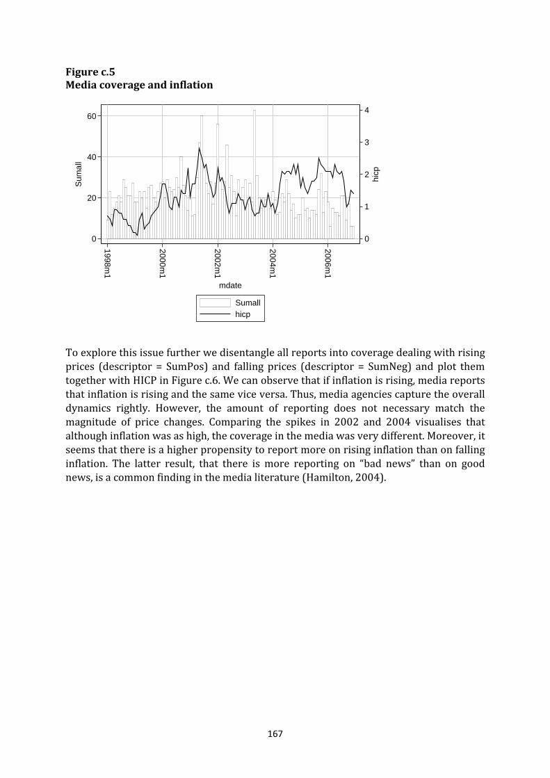
Figure c.5 Media coverage and inflation

0

1

2

3

4

hicp

0

20

40

60

Sum

all

1998m1

2000m1

2002m1

2004m1

2006m1

mdate

Sumallhicp To explore this issue further we disentangle all reports into coverage dealing with rising prices (descriptor = SumPos) and falling prices (descriptor = SumNeg) and plot them together with HICP in Figure c.6. We can observe that if inflation is rising, media reports that inflation is rising and the same vice versa. Thus, media agencies capture the overall dynamics rightly. However, the amount of reporting does not necessary match the magnitude of price changes. Comparing the spikes in 2002 and 2004 visualises that although inflation was as high, the coverage in the media was very different. Moreover, it seems that there is a higher propensity to report more on rising inflation than on falling inflation. The latter result, that there is more reporting on “bad news” than on good news, is a common finding in the media literature (Hamilton, 2004).

167

Figure c.6 Media coverage and inflation (positive versus negative news)

0

1

2

3

4

hicp

−20

0

20

40

1998m1

2000m1

2002m1

2004m1

2006m1

mdate

SumPosSumNeghicp As our main variable in focus is inflation perception we now plot the media data (descriptor = SumAll) against the inflation perception series in Figure c.7. As we can see there are some incidences where high coverage is correlated with substantial increases in the perception measure for instance 2001 and 2002. However, the high coverage in the beginning of 2003 is followed by a decrease in inflation perceptions. To analyse the issue further we disentangle the amount of reporting into news on rising (descriptor = SumPos) and falling inflation (descriptor = SumNeg) as shown in Figure c.8. While the increases in 2001 and 2002 are driven by reporting on rising inflation indeed the fall in 2003 is triggered by news on falling inflation. As the impact on inflation perceptions seems to be rather asymmetrically distributed, we decided to include the media variables into our regression setup separately.

168

Figure c.7 Media coverage (amount) and perceptions

0

20

40

60

80

Per

cept

ion

0

20

40

60

Sum

all

1998m1

2000m1

2002m1

2004m1

2006m1

mdate

SumallPerception

Figure c.8 Media coverage (tone) and perceptions

0

20

40

60

80

Per

cept

ion

−20

0

20

401998m

1

2000m1

2002m1

2004m1

2006m1

mdate

SumPosSumNegPerception

169

Finally, we employ the measure extracted from the LexisNexis database and counting the articles containing the wording “teuro” and “euro changeover“. Figure c.9 shows the relationship between teuro and inflation perceptions. The sharp rise in inflation perception corresponds with the repeatedly wording of “teuro”. Figure c.9 Teuro and perceptions

0

20

40

60

80

Per

cept

ion

0

50

100

150

200

Teu

ro

1998m1

2000m1

2002m1

2004m1

2006m1

mdate

TeuroPerception We start the formal econometric analysis with the setup of the entry regressions from section c.3.i and include our media variables systematically (table c.2). In column (1) we add both count variables. While the regressors from the entry regressions remain stable, the variable accounting for the “teuro” debate has a significant positive impact on inflation perceptions. This is reasonable as there the main message of those articles was indeed to ”warn” the public of rising prices with respect to the introduction of the euro. Notably the discussion on the euro introduction itself reveals no such impact. As the HICP becomes insignificant, this implies that people obtain their information from the media and the inflation figure itself does not have significant additional information

170

value (see Curtin, 2007 and Blinder and Krueger, 2004). In column (2) we introduce media variables that capture, how much articles report rising inflation and how much report falling inflation. Notably, only news on rising inflation seems to matter for the public as it increases the perceptions – there is a clear asymmetry. Furthermore, HICP does not add any explanatory power if media variables are included. Thus, all necessary information is provided by media agencies which explain the figure and draw implications. Note that this result is not influenced by multicollinearity among the regressors as the correlation between the regressors is well below 0.6. In columns (3) and (4) we split the sample again. Interestingly, media had no explanatory power before the introduction of the euro. Obviously there was no

additional information provided by media companies that could not also be inferred by looking at the index figure of the HICP. In harsh contrast, after the introduction of the euro, consumers heavily relied on their past expectations as well as on the information provided by the media. This is in line with "agenda-setting approaches" which would imply a threshold effect – once the reporting on a certain topic achieves certain e "issue" and remains visible foint nsity, it is perceived as an r a longer time. In column (5) we address the endogeneity issue between perceptions and media reporting. One might argue that agencies might cater to the prejudice of their readers and therefore react to inflation perceptions. For this purpose we employ three stage least squares (3SLS) techniques, instrumenting the media variables with their own lags.22 Notably the results are unaffected and the coefficient estimate even increases in its magnitude. Table c.8 Media and perceptions

(1) (2) (3) (4) (5) <2002 >2002 3SLS

L.Perception 0.891*** 0.925*** 0.775*** 0.939*** 0.927***(0.032) (0.025) (0.069) (0.036) (0.024)

L6.Expectation 0.161*** 0.162*** 0.002 0.166*** 0.171***(0.050) (0.039) (0.082) (0.038) (0.050)

hicp 2.494*** 0.547 4.969*** 1.005 0.002(0.716) (0.570) (1.547) (0.983) (1.050)

teuro 0.036***(0.013)

euro 0.002(0.025)

sumpos 0.169** 0.058 0.190*** 0.251**(0.082) (0.108) (0.068) (0.122)

sumneg -0.054 -0.083 0.078 -0.182(0.081) (0.100) (0.131) (0.203)

changeoverdummydoehring 1.646 2.888** 2.950**(1.575) (1.104) (1.184)

Constant -5.293*** -4.770*** -0.725 -3.854 -4.255**(1.738) (1.423) (2.403) (2.409) (1.764)

Observations 101 102 42 60 102Robust standard errors in parentheses*** p<0.01, ** p<0.05, * p<0.1 Similar to the exercise performed for the entry regression, we report the impact of each variable on inflation perceptions based on the impulse of a shock of one unit standard eviation. While Figure c.10 seems very similar to Figure c.3 it contains on interesting d

171

22 The method 3SLS is similar to two-stage least squares (2SLS/TSLS) but involves an estimation of the variance-covariance matrix. Similar as in seemingly unrelated regression (SUR) models, the 3SLS makes use of the cross-equations correlation of the disturbances. Thus, in comparison to 2SLS, 3SLS is more efficient, a relative advantage that increases with the strength of the interrelations among the error terms. 3SLS is equivalent to a GMM approach if the errors are homoscedastic.

further feature. The response to the “positive news” (= increasing inflation) variable is found to be much higher compared to the remaining explanatory variables. Thus, not only are media reports statistically significant but also economically important as the outreach any other variable put into this regression. Figure c.10 Impulse response of inflation perceptions after one S.D. shock

0

2

4

6

8

10

12

14

16

18

20

Perception Expectation hicp sumpos sumneg To fully account for the dynamics between the different variables, especially perceived inflation and media, we employ a vector autoregression (VAR) setup. As variables that are endogenous we define perceived inflation and the media variables. Exogenous variables are the six-month lag of expectations, HICP and the changeover dummy. We also tested monthly as well as yearly dummies. Notably, monthly dummies have no effect. We use four lags since the common lag selection criteria were inconclusive. Results are presented in Tables c.9 and c.10. Table c.9 shows the regression estimates while in Table c.10 the associated Granger causality tests are presented. From Table c.10 we can extract that lagged media variable significantly affects perceptions but the reverse causality link is not statistically significant. This implies that although reverse causality might be rational and present it does not drive our results as the main channel is the link from media to inflation perceptions.

172

Table c.9 Vector Autoregression

(1) (2) (3) Perception sumpos sumneg

L.Perception 0.803*** 0.311* -0.154(0.105) (0.161) (0.118)

L2.Perception 0.199 -0.228 -0.013(0.135) (0.207) (0.152)

L3.Perception 0.087 0.055 0.173(0.136) (0.209) (0.153)

L4.Perception -0.144 -0.067 -0.004(0.100) (0.154) (0.113)

L.sumpos 0.126* 0.378*** 0.099(0.066) (0.102) (0.074)

L2.sumpos -0.102 -0.437*** 0.148*(0.071) (0.110) (0.080)

L3.sumpos -0.038 0.115 -0.076(0.072) (0.110) (0.081)

L4.sumpos -0.102* -0.287*** 0.125*(0.061) (0.094) (0.069)

L.sumneg -0.121 -0.179 0.406***(0.097) (0.149) (0.109)

L2.sumneg 0.104 0.267* -0.059(0.105) (0.161) (0.118)

L3.sumneg -0.113 -0.125 -0.016(0.105) (0.161) (0.118)

L4.sumneg 0.129 -0.067 0.148(0.099) (0.151) (0.111)

L6.Expectation 0.183*** 0.088 0.075(0.049) (0.076) (0.055)

changeoverdummydoehring 1.765 -5.160*** 0.568(1.173) (1.803) (1.318)

hicp 2.367*** 7.089*** -2.745***(0.836) (1.285) (0.940)

Constant -5.947*** -1.473 2.114(1.704) (2.619) (1.915)

Observations 102 102 102Standard errors in parentheses*** p<0.01, ** p<0.05, * p<0.1

Table c.10

Equation Excluded F df df_r Prob > FPerception sumpos 2.513013 4 86 0.047426Perception sumneg 0.972532 4 86 0.426892Perception ALL 2.213312 8 86 0.033987sumpos Perception 1.528253 4 86 0.201143sumpos sumneg 0.971349 4 86 0.427536sumpos ALL 1.174841 8 86 0.323649sumneg Perception 0.893416 4 86 0.471559sumneg sumpos 2.59415 4 86 0.041989sumneg ALL 1.684462 8 86 0.113721

173

Finally, we condition the results on the socioeconomic characteristics of the respondents. Results are presented in Table c.11. Variable Definitions are reported in the Appendix. The regressions represent mainly regressions estimated in Tables c.1 and c.2 – the main difference being that we use balance statistics calculated for certain groups separately. Note that we refrain from considering employment characteristics and focus on gender, earnings, education and age. While earlier studies have been quite clear that the uneducated, poor and older people have problems inferring the accurate inflation rate our results are less clear cut. Formally, there is no statistically different response. Nevertheless, some patterns emerge. For instance, the more educated people are the stronger is the link between HICP and inflation perceptions. Those groups also react to news on the "teuro" as well to news on rising inflation. On the positive side this implies that they strongly update on existing statistical figures. On the negative side, especially in the aftermath of the euro introduction they also reacted strongly to media reporting. With respect to gender, the estimated coefficients are very similar independent of the regression setup. With respect to income and age no linear trend is observable. Concerning age it seems that there is some inverted u-shape relationship between information income and perceptions. Those active in the workforce seem to respond stronger to news on inflation and published inflation numbers. Concerning income those in the 3rd income quartile respond most to news on inflation as well as HICP. These results are partly surprising as one could have expected that for instance most educated people would have not responded to the “teuro” debate.

174

(1)(2)

(3)(4)

(5)(6)

(7)(8)

(9)(10)

(11)(12)

(13)(14)

detot5

bsmdere15b

smdere25bs

mdere35bsm

dere45bsmd

eed15bsmde

ed25bsmdee

d35bsmdeag15

bsmdeag25b

smdeag35bs

mdeag45bs

mdemal5bsm

defem5bsm

hicp1.826*

**1.898*

*1.763*

2.031**

1.718*1.516*

*2.039*

*2.778*

*1.425*

*2.085*

*1.976*

*1.504*

*1.847*

**1.822*

*(0.686

)(0.906)

(0.946)

(1.005)

(0.902)

(0.648)

(0.789)

(1.382)

(0.639)

(0.850)

(0.779)

(0.737)

(0.693)

(0.748)

changeover

0.9351.009

1.5011.536

1.5620.926

1.3410.494

1.4711.095

1.3451.065

1.0121.109

(1.153)(

1.316)(1.471

)(1.595

)(1.451

)(1.255

)(1.250

)(1.859

)(1.345

)(1.325

)(1.188

)(1.379

)(1.166

)(1.282

)hicp

2.494***2

.689***2.950*

**3.282***

2.315**2

.158***2.853*

**3.724*

*2.012*

**2.804*

**2.887*

**2.224*

**2.591*

**2.494*

**(0.716

)(0.974)

(1.050)

(1.064)

(0.993)

(0.689)

(0.826)

(1.470)

(0.656)

(0.900)

(0.804)

(0.804)

(0.713)

(0.802)

teuro0.036*

**0.042*

*0.075**

0.067***

0.039*0.035*

*0.045*

**0.072*

**0.036*

0.042***

0.054***

0.029**

0.038***

0.040***

(0.013)(

0.021)(0.030

)(0.021

)(0.020

)(0.015

)(0.016

)(0.027

)(0.019

)(0.015

)(0.019

)(0.014

)(0.014

)(0.015

)euro

0.002-0.007

0.0230.026

0.0130.014

-0.0080.052

-0.0070.005

0.021-0.010

-0.0000.007

(0.025)(

0.023)(0.031

)(0.035

)(0.038

)(0.023

)(0.027

)(0.041

)(0.026

)(0.025

)(0.028

)(0.035

)(0.033

)(0.026

)change

over1.646

1.9621.133

2.2902.497

2.0821.669

0.6632.031

1.8212.416

1.2661.909

1.623(1.575

)(1.508)

(2.112)

(1.870)

(1.896)

(1.632)

(1.687)

(2.410)

(1.693)

(1.740)

(1.562)

(1.992)

(1.642)

(1.633)

hicp0.547

0.9350.195

0.7070.216

0.5170.664

0.5080.174

1.1370.321

0.2490.347

0.768(0.570

)(0.770)

(1.092)

(0.994)

(0.883)

(0.677)

(0.692)

(1.280)

(0.650)

(0.734)

(0.742)

(0.851)

(0.647)

(0.650)

sumpos

0.169**

0.1540.202*

0.213**

0.184*0.160*

*0.186*

*0.236

0.189**

0.1380.219*

**0.151*

0.192**

0.155*(0.082

)(0.095)

(0.103)

(0.097)

(0.108)

(0.073)

(0.089)

(0.163)

(0.083)

(0.094)

(0.077)

(0.089)

(0.081)

(0.089)

sumneg

-0.0540.002

-0.0530.003

-0.076-0.013

-0.038-0.175

0.007-0.029

-0.065-0.107

-0.078-0.015

(0.081)(

0.101)(0.127

)(0.115

)(0.118

)(0.076

)(0.094

)(0.162

)(0.106

)(0.093

)(0.088

)(0.114

)(0.081

)(0.095

)change

over2.888*

*3.069**

3.138*3.868*

*3.527*

*3.237***

3.136**

2.1213.209*

*3.169*

*3.665*

**2.648*

3.077***

2.994**

(1.104)(

1.245)(1.625

)(1.497

)(1.406

)(1.178

)(1.245

)(1.891

)(1.346

)(1.260

)(1.205

)(1.466

)(1.156

)(1.234

)<2002 hicp

4.969***6

.499***4.142

5.517**7

.065***4.899*

**5.587*

**7.036*

*4.922*

**6.547*

**5.060*

**4.109*

4.513***

5.868***

(1.547)(

1.640)(2.501

)(2.592

)(1.992

)(1.375

)(1.747

)(3.187

)(1.604

)(1.761

)(1.758

)(2.233

)(1.520

)(1.713

)sumpo

s0.058

0.0680.040

0.1060.029

0.0520.052

0.0200.012

0.0420.115

-0.0090.061

0.054(0.108

)(0.130)

(0.153)

(0.131)

(0.118)

(0.099)

(0.102)

(0.206)

(0.102)

(0.118)

(0.098)

(0.103)

(0.094)

(0.120)

sumneg

-0.083-0.013

-0.171-0.159

-0.131-0.037

-0.102-0.199

-0.077-0.009

-0.146-0.195

-0.1510.004

(0.100)(

0.120)(0.188

)(0.135

)(0.145

)(0.098

)(0.107

)(0.192

)(0.124

)(0.110

)(0.122

)(0.139

)(0.095

)(0.122

)>=2002 hicp

1.0050.719

-0.2811.784

0.0010.328

1.2950.118

0.2271.642

0.3230.685

0.9460.832

(0.983)(

1.537)(1.849

)(1.681

)(1.642

)(1.255

)(1.290

)(2.308

)(0.924

)(1.461

)(1.298

)(1.092

)(1.064

)(1.142

)sumpo

s0.190*

**0.136*

0.273***

0.209*0.261*

*0.160*

0.220***

0.365***

0.228***

0.1190.255*

**0.222*

**0.246*

**0.144*

(0.068)(

0.080)(0.094

)(0.112

)(0.110

)(0.088

)(0.072

)(0.124

)(0.064

)(0.106

)(0.075

)(0.080

)(0.071

)(0.072

)sumne

g0.078

0.1440.196

0.227-0.003

0.1330.136

-0.1370.251

0.1190.032

0.0090.029

0.150(0.131

)(0.202)

(0.189)

(0.189)

(0.180)

(0.130)

(0.151)

(0.284)

(0.172)

(0.149)

(0.131)

(0.176)

(0.116)

(0.170)

Tab

le c

.11

So

cioe

con

omic

ch

arac

teri

stic

s an

d in

flat

ion

per

cep

tion

s

175

References Aucremanne, Luc, Collin, Marianne, and Thomas Stragier (2007): “Assessing the gap between observed and perceived inflation in the euro area: is the credibility of the HICP at stake?”, National Bank of Belgium Working papers series, No. 122, April. Blanchflower, David G. and Roger Kelly (2008): Macroeconomic Literacy, Numeracy and the Implications for Monetary Policy, Working Paper. Blinder, Alan and Krueger, Alan B. (2004): What Does the Public Know about Economic Policy, and How Does It Know It?, CEPS Working Paper 99. Brachinger, Hans W. (2006): Euro or ‘Teuro’? The Euro-induced Perceived Inflation in Germany”. Department of Quantitative Economics Working Paper No. 5. University of Fribourg. Bryan, Michael F. and Palmqvist, Stefan (2005): Testing Near-Rationality Using Detailed Survey Data, Working Paper 0502, Federal Reserve Bank of Cleveland. Bryan, Michael F. and Venkatu, Guhan (2001): The Demographics of Inflation Opinion Surveys, Economic Commentary, Federal Reserve Bank of Cleveland. Burgoyne, Carole B., Routh, D. A. and Ellis, A.-M. (1999): The Transition to the Euro: , 22. Some Perspectives from Economic Psychology. Journal of Consumer PolicyCarlson, John A. and Parkin, J, Michael, (1975): Inflation expectations. Economica, 42(166):123–138. eo. Curtin, Richard (2007): What U.S. Consumers Know About Economic Conditions, mimCestari, Vincenzo, Del Giovane, Paolo, and Clelia Rossi-Arnaud (2007): “Memory for prices and the euro cash changeover: an analysis for cinema prices in Italy”, Banca d’Italia, Temi di Discussione, 619, February. Del Giovane, Paolo and Sabbatini Roberto (2006): Perceived and measured inflation after the launch of the euro: explaining the gap in Italy, Giornale degli Economisti e Annali di Economia, 65 (2), 155–192. Del Giovane, Paolo, Silvia Fabiani and Roberto Sabbatini (2008): What's behind "inflation perceptions"? A survey-based analysis of Italian consumers. Bank of Italy Temi di Discussione (Working Paper) No. 655 Döhring, Björn and Mordonu, Aurora (2007): What Drives Inflation Perceptions? A

176

No 458. Ehrmann, Michael (2006): Rational Inattention, Inflation Developments and Perceptions after the Euro Cash Changeover. Working Paper 588, European Central Bank.

Dynamic Panel Data Analysis, Economic Papers 284. Dziuda, Wioletta and Mastrobuoni, Giovanni (2006): The Euro Changeover and Its Effects on Price Transparency and Inflation, Collegio Carlo Alberto Working Paper. Eife, Thomas A. and Coombs, W. Timothy (2007): Coping with People’s Inflation Perceptions During a Currency Changeover, Heidelberg Discussion Paper Series

Fluch, Manfred and Stix, Helmut (2005): Perceived Inflation in Austria – Extent, Explanations, Effects, Monetary Policy & the Economy (3): 22–47. Forsells, Magnus and Kenny, Geoff (2004): Survey Expectations, Rationality and the Dynamics of Euro Area Inflation, Journal of Business Cycle Measurement and Analysis, 1 (1): 13–41. Hamilton, James T. (2004): All the News That’s Fit to Sell: How the Market Transforms Information into News. Princeton University Press, Princeton, N.J. Hofmann, Eva, Kamleitner, Bernadette, Kirchler, Erich. and Schulz-Hardt, Stefan (2001): Kaufkraftschwund nach der Währungsumstellung: Zur erwartungsgeleiteten Wahrnehmung des (T)Euro, Wirtschaftspsychologie 1. Inoue, Atsushi, Kilian, Lutz and Kiraz, Fatma B. (2006): Do Actions Speak Louder than Words? Household Expectations of Inflation Based on Micro Consumption Data, CEPR Discussion Paper 5790. Jungermann, Helmut, Hans W. Brachinger, Julia Belting, Katarzyna G. and Elisabeth Zacharias (2007): The Euro Changeover and the Factors Influencing Perceived Inflation, Journal of Consumer Policy, 30:405–419. Kahnemann, Daniel and Tversky, Amos (1979): Prospect Theory: An Analysis of Decision under Risk, Econometrica. Lamla, Michael and Lein, Sarah. (2008): The Role of Media for Consumers' Inflation Expectation Formation, KOF Working Paper No 201. Lein, Sarah and Maag, T. (2008): The Stickiness of Inflation Perceptions: Some Evidence for European Countries, KOF ETH Zurich. Malgarini, Marco (2007): “Quantitative inflation perceptions and expectations of Italian consumers”, ISAE, mimeo. Palmqvist, Stefan and Lena Strömberg (2004): Households’ inflation opinions – a tale of two surveys, Sveriges Riksbank Economic Review 2004:4. Sims, Christopher (2003): Implications of Rational Inattention, Journal of Monetary Economics, 50 (3):665–690. Stix, Helmut (2006): Perceived Inflation and the Euro: Why High? Why Persistent? Beitrag zur Jahrestagung der European Economic Association. Wien. Traut-Mattausch, Eva, Schulz-Hardt, Stephan, Greitemayer, Tobias and Frey, Dieter (2004): Expectancy Confirmation in Spite of Disconfirming Evidence: The Case of Price Increases Due to the Introduction of the Euro, European Journal of Social Psychology, No. 34, 739–760.

177

Appendix

Table c.A.1 Definition socioeconomic characteristics

Socio Economic CharacteristicsCode Consumer categories

TOT Total of the sample

Income of the HouseholdRE1 1st QuartileRE2 2nd QuartileRE3 3rd QuartileRE4 4th Quartile

Education of respondentED1 PrimaryED2 SecondaryED3 Further

Age of respondentAG1 16-29AG2 30-49AG3 50-64AG4 65+

Sex of respondentMAL MaleFEM Female

Table c.A.2 Country Abbreviations

178

Code Country Name

EA Euro areaAT AustriaBE BelgiumCY CyprusDE GermanyEL GreeceES SpainFI FinlandFR FranceIE IrelandIT ItalyNL NetherlandsSI Slovenia SE SwedenUK United Kingdom

179analyse each product group separately We summarise our results in the following Table d.S.1. A “X” means that we find evidence for convergence in the respective group and country aggregate. We conclude

d) Cross-border convergence of prices since the euro changeover

Summary We begin our empirical analysis by comparing the dynamics of product prices across countries. In particular, we aim to analyse whether the changeover to the euro has been accompanied by an increase in market integration and, thus, a decline in price dispersion among member countries of EMU. To do so, we essentially borrow two econometric techniques from the literature on economic growth to estimate the extent of convergence. The concept of β-convergence implies that countries with a lower initial level of prices experience faster subsequent increases in the price level (i.e., higher inflation). This implication is usually tested by regressing the change in prices on the initial price level. A negative correlation would then indicate that prices grow on average slower when they are initially high and vice versa. The second concept, σ-convergence, implies a decrease in the dispersion of price levels across countries. We test for this type of convergence by regressing a measure of price dispersion on a trend variable. Again, we would expect a negative coefficient if there is evidence of σ- price convergence. Whereas beta convergence only implies that countries with initially low price levels grow faster, σ- convergence implies that the countries´ prices converge to the same level. Hence, β-convergence is the weaker concept, in the sense that we could find β-convergence, i.e. countries with high price levels experience lower growth rates of price levels and countries with low price levels experience high growth rates, but that they do not converge to the same price level, which means that we do not observe sigma convergence. On the other hand, if we observe that price dispersion decreases (σ-convergence), we must also observe β-convergence. Thus, σ-convergence implies β-c s convergence, but not vi e ver a. We disaggregate the data in several ways. We distinguish three dimensions of disaggregation: First, we look at the country aggregate dimension (that is, we analyse EMU countries and non-EMU countries separately). If we find convergence in EMU but also in non-EMU countries, we do not treat the convergence as a result of the euro introduction, because it might be due to other factors, which also affect non-EMU countries. Second, we look at the time dimension. For β-convergence, we take the period 2001 as the initial price level and analyse whether we find evidence for β-convergence after the euro cash changeover in January 2002. Third, we look at the aggregation of the product groups to compare whether some product groups might show more or less convergence than others. We first aggregate all products together and then disaggregate the products into different groups and, finally,

180

that we find evidence for a euro changeover induced convergence if (i) we find convergence after 2001 for β-convergence and significantly faster convergence after 2001 in the case of σ-convergence; (ii) we do not find convergence for the respective product group in non-EMU countries and (iii) as σ-convergence implies β-convergence but not vice versa, we consider evidence for σ-convergence as robust only if there is also evidence for β-convergence for the respective product group. Looking at the summary table, we see that for the aggregation over all products, we find no evidence for convergence due to the euro cash changeover. The same is true for tradables and nontradables. For perishable foods we find evidence for β-convergence in EMU after 2001. For the category communication we also find β-convergence for the EMU. The category “recreation and culture” shows both β-and σ-convergence in the case of EMU countries, but only β-convergence in non-EMU countries. Hence, according to our definition of euro induced price convergence, σ-convergence is special in this category for EMU countries. We also find β-convergence in “housing”. However, the change in housing prices might largely drive that result, which is rather unlikely to be related to the euro introduction. For the single product groups we find evidence for σ-and β-convergence only for the products “lamb, mutton and goat” and “jewellery, clocks and watches”. Evidence for β-convergence can be found in the product groups “fresh milk” ,”tobacco”, “bedroom furniture”, “small electric household appliances”, “domestic services (non-tradable)” and “motor cars with petrol engine of cubic capacity of less than 1200cc”. Hence, our results do not support that price dispersion has significantly decreased due to the introduction of a single currency for most product groups, with a few exceptions listed above. However, one should bear in mind that the period for analysis is still relatively short: after the euro introduction we have only four years of observations. Hence, we might have to obtain more data to find more statistical evidence for price convergence.

181

Table d.S.1

EMU Non-EMU

Group β-convergence,after 001 2 σ-convergence,after 001 2 β-convergence, after 001 2 σ-convergence,after 001 2All X X Tradable X X Nontradable X X Alcohol an(at) d tobacco X Electrical appliances (ea) Food: non-perishable (fn) X Food: perishable (fp) X Alcoholic X Clothing Communication X Education X Food X Furnishings Health Housing X X Misc. Recreation X X X Restaurants Transport Other cereals d (except rice) anflour (1101112) X Pasta products (1101115) X Lamb, mutt(1101123) on, goat X X Fresh milk (1101141) X Tobacco (1102211) X Children’s and infant’s clothing (1103123) X X Actual rentals for housing (1104111) X X Bedroom furn(1105112) iture X Small electric plian-household apces (1105321) X Non-durable household goods (1105611) X

182

Domestic service(1105621) s X Motor cars with petrol engine less than 1200cc (1107112) X Books (1109511) X Pubs, bars, cafés, tea rooms and thelike (1111112) X Jewellery, clocks nd watches 1112311) a( X X

183d.1.1) Market integration and prices The literature on the ‘border effect’ in prices begins with a puzzling empirical finding. In a path-breaking study, Engel and Rogers (1996) explore consumer price data from 23

d.0) Introduction In this chapter, we analyse the extent of cross-border price convergence among EMU member countries after the introduction of the euro. The chapter is organised as follows. Section d.1) reviews the existing literature. In Section d.2), we briefly describe the price data that we use in our empirical analysis. Section d.3) applies various standard techniques to examine prices level convergence for up to 224 product groups. Finally, we examine possible factors that drive the speed of price convergence. In an appendix, we also provide a set of preliminary results of a differences-in-differences analysis to identify (directly) a possible effect of the euro cash changeover on price dispersion. d.1) Survey of the literature on price level convergence under EMU A number of studies have already empirically analysed the effect of the euro on prices. Broadly, there are three groups of recent works that deal with this issue. A first set of papers is mainly concerned with the ‘border effect’, i.e., the finding that prices vary more significantly across borders than for pairs of cities located within the same country, after holding constant for other factors. Since a potential explanation for this discrepancy may be the use of separate national currencies in different countries, these papers aim to identify the effect of sharing a single currency (i.e., membership in a currency union) on price differentials. In this respect, the formation of EMU provides an almost perfect ‘natural experiment’ to analyse this issue. A second set of papers is mainly concerned with the extent of market integration in the European Union. The formation of the ‘Single European Market’ in 1993 aims to remove, among other things, any remaining barriers to the movement of goods. Analysing the evolution of price dispersion within the European Union then allows tracking the success of these policies; lower barriers to trade should be associated with smaller price differentials. With the introduction of the euro, simply another dimension is added in these studies. In contrast to other work that often explores price convergence for a broad range of products, most of the papers in this strand of the literature analyse the price differentials on a particular product market (of interest), such as the European car market. Finally, there are a growing number of papers that focus directly on the euro’s effect on prices. Apart from the fact that this is an interesting research question in itself, these papers mainly contribute to the larger literature on the effects of the euro on economic activity. Most notably, this work complements extensive research on the euro’s effects on trade. In the following, we discuss these strands of the literature in more detail.

184

s

North American cities (of which 14 cities were located in the United States, while the remaining 9 cities were located in Canada) for 14 disaggregated product categories. Since Engel and Rogers (1996) examine price indexes, they do not observe price differentials directly, but instead compute the bilateral price volatility (i.e., the standard deviation of the two-month difference in the log of the price in location i relative to the price of the good in location j) for any pair of cities. Not surprisingly, Engel and Rogers (1996) find that a significant part of the observed variation in prices is explained by the geographical distance between cities; cities that are further apart tend to display larger price variabilities. More importantly, however, Engel and Rogers (1996) also find that consumer prices were significantly more variable (by a huge margin) for pairs of cities located across the U.S.-Canadian border than for pairs of cities located within the same country, even after controlling for the effect of distance. As a result, Rogoff (1996, p. 665) concludes that “[i]nternational goods markets are highly integrated, but not yet nearly as integrated as domestic goods markets”. Puzzled by the Engel and Rogers (1996) finding, a number of authors have aimed to analyse international price differentials in more detail. A major difficulty for this type of analysis is the availability of usable data. In principle, the price data should display the following features: (i) the product definitions should be identical across locations (otherwise prices are hardly comparable); (ii) the price data should be in levels rather than indexes (otherwise only second moments can be analysed); and (iii) the data set should comprise both national and international locations (otherwise it is impossible to identify a ‘border effect’). One of the rare data sets that meet all of those requirements is the City Data database which is compiled by the Economist Intelligence Unit (EIU). This database contains price information for 160 (well-defined) products and services across 123 cities in 79 countries.22 Based on this information, the bilateral price differential can be easily computed for any pair of cities. Potential determinants of price dispersion are then analysed in a gravity-type regression that includes controls for, among others, cities located in the same country, bilateral distance, common language and historical links. Most importantly, since some of the cities in the EIU database are located in countries that are member of the same currency union, the regression framework allows identifying the effect of using a single currency on price differentials.23 Parsley and Wei (2001) apply this approach to exploit a sub-set of the EIU data. Their ample includes only one city per country (except for the United States) and (potential) 22 The EIU markets this database mainly for marketing managers (who need to compare operational costs and pricing policies where they do business), business travellers (in order to determine costs of overseas visits), and human resources officers (who need to design compensation packages for expatriate staff). ts to record price levels; Prices are collected twice a year by local researchers who physically visit outlesee: http://www.eiu.com/site_info.asp?info_name=ps_cityData&entry1=psNav&rf=0. 23 Apart from cities in EMU member countries, the City Data database comprises cities in member countries of the CFA franc zone (Cameroon, Cote d’Ivoire, Gabon, Senegal) as well as some dollarized countries (Ecuador, Panama).

185

traded goods for which more than 70 percent of the observations are non-missing; in total, their sample comprises prices for 95 goods and 83 cities for the period from 1990 to 2000. Parsley and Wei (2001) briefly discuss possible measures of price dispersion. For illustration, they display absolute percentage price deviations for a small group of selected goods and city pairs.24 In their empirical analysis, however, they use the standard deviation of the (good-specific and time-specific de-meaned) price differential as dependent variable. In particular, they note that the variation in the absolute price differential provides no useful information as long as the differential is less than the cost of arbitrage so that they focus instead on the dispersion of the price differential, arguing that any movement toward market integration should reduce the no-arbitrage range. Parsley and Wei (2001) find that, on average, currency arrangements significantly reduce the dispersion of relative prices, even after controlling for the effect exchange rate variability. Parsley and Wei distinguish for the effects of various currency arrangements, including the adoption of the euro. Not surprisingly, they find the strongest reduction in price dispersion for cities located within the United States (thereby reflecting the ‘border effect’). Considerably smaller though still significant effects are reported for ‘hard pegs’ (which are, in the Parsley and Wei sample, essentially currency board linkages to the US dollar) and the euro area. The point estimates suggest that membership in these arrangements is associated with a reduction in price dispersion by about 3 percent. Membership in the CFA franc zone, in contrast, has no measurable effect on price dispersion. Parsley and Wei (2001) also provide extensive sensitivity checks of their results. Two findings appear particularly noteworthy. First, the euro effect disappears once the year fixed effects are replaced with a trend dummy; that is, there is a considerable decline in price dispersion among EMU member countries already before the formation of EMU, with no separate effect after the adoption of the euro (though it should be noted that Parsley and Wei have only two years of data from EMU). Second, the results are robust to variations in the measure of price dispersion. Parsley and Wei substitute the standard deviation of the differences in prices with the difference between the 75th and the 25th percentile of the distribution of percentage price differences and the standard deviation of the absolute differences in prices. For both perturbations, the main findings remain qualitatively unchanged. Another paper that exploits the EIU data to examine the effect of currency arrangements on prices is Isgut (2004). The setup is basically identical to Parsley and Wei (2001), except that Isgut explores the dispersion of prices for a larger number of goods and cities, but one year (2001) only. The results are basically similar to the findings in Parsley and Wei (2001). Sharing the same currency leads to a reduction of about 3 percent in the standard deviation of log price differences across city pairs, which represents about one third of the ‘same country’ effect. In contrast to Parsley and Wei, however, Isgut (2004) finds, among the currency areas in his sample, the strongest effect or the use of the euro (on the order of around 5 percent), which may be due to the arger number of cities from EMU countries in his sample. Interestingly, Isgut also fl 24 The percentage price difference for a given city pair i,j and a given product k at time t is defined as: Qij,k,t = ln Pi,k,t – ln Pj,k,t, where Pi,k,t denotes the US dollar price of good k in city i at time t.

186

the establishment of the EMU. Similar to Goldberg and Verboven (2004), Gil-Pareja and Sosvilla-Rivero (2008) extend earlier work on price convergence in the European car market (Sosvilla-Rivero and Gil-Pareja, 2004) to analyse the evolution of price dispersion in the EMU. Gil-Pareja and Sosvilla-Rivero use essentially the same car price data as Goldberg and Verboven, but include more recent data (covering the period until 2005) and use the coefficient of

provides a comparison of price differentials for tradables and nontradables. As expected, he finds no effect of currency arrangements on the dispersion of prices for nontradables, although other determinants, such as the bilateral distance between cities, are still found to be significant. d.1.2) Price convergence in the European Union A sizable literature is mainly concerned with the extent of market integration in the European Union. These papers typically focus on deviations from the Law of One Price for individual markets; they can easily be extended to cover also market integration in EMU. A case in point is the series of papers by Goldberg and Verboven (2004, 2005) on the European car market. In Goldberg and Verboven (2004), the authors examine car price data for about 90 models sold during the period 1993 to 2003 in the 15 member countries of the European Union (at the time of publication); the data are collected bi-annually by the European Commission. In order to identify the impact of the euro on cross-country price dispersion, they examine the absolute values of the (pre-tax car) price differences relative to the Netherlands. They employ a difference-in-differences analysis; that is, they examine the change in the price difference for EMU member countries after the introduction of the euro, using (the three) non-participating EU countries as control group. Goldberg and Verboven (2004) find that price differentials in EMU member countries over the whole sample period (1993–2003) were on average lower by about 6 percent compared to price differentials of non-EMU member countries, perhaps reflecting lower exchange rate volatility among EMU members even before the introduction of the euro. More importantly, Goldberg and Verboven find that price differentials have decreased by about 1.4 percent after the launch of the monetary union in 1999, while price differentials in non-EMU countries have marginally increased (by about 0.5 percentage points). A different, much more diverse picture emerges when the periods of monetary union (1999–2001) and currency union (2002–2003) are examined separately. While price differentials within EMU appear to have continuously declined over both periods, price differentials in non-EMU member countries have widened until 2001 and then reverted back to the pre-1999 levels in the last two years of the sample. Moreover, price movements in non-EMU member countries are entirely driven by the experiences of the United Kingdom and Sweden; for Denmark, price dispersion has declined in both sub-periods, suggesting that also non-members can benefit from the monetary union (by fixing their exchange rate to the new currency). In a dynamic specification, where the dependent variable is the first difference of the log-price difference relative to the Netherlands, Goldberg and Verboven (2004) find that EMU member countries display on average a higher speed of convergence than non-EMU members; that is, after a temporary shock, intra-EMU price differentials revert back to their long-term levels faster than price differentials that involve non-EMU members. Still, there is no measurable difference in the change of the speed of convergence after

187EMU countries, and controlling for other factors that may affect price dispersi n. Rogers (2007) is a recent update of the analysis in Engel and Rogers (2004). In particular, Rogers provides three extensions. First, another year of data (2004) is added. Second, the measure of dispersion is the standard deviation of a price index that is a

variation (i.e., the ratio of the standard deviation to the mean) as their measure of price dispersion. Applying the concept of σ-convergence, this measure is then regressed on a simple time trend; the regression is performed, individually for 45 car models, for different samples of countries and periods. Comparing the estimated coefficients, Gil-Pareja and Sosvilla-Rivero (2008) find a measurable difference in the patterns of price convergence between EU and EMU member countries before the establishment of EMU, with (future) EMU member countries displaying convergence, while there is no sizable reduction in price dispersion for EU countries as a whole. After the formation of EMU, in contrast, there is evidence of price convergence for both groups of countries. However, if anything, there is more evidence of convergence among the EU than among EMU countries, which may be partly explained by the much larger dispersion of prices within the European Union at the beginning of the period. As a result, Gil-Pareja and Sosvilla-Rivero (2008, p. 249) conclude that “the decline in price dispersion cannot be attributed, at least only, to the euro.” Price differentials for another product, TV sets, have been analysed by Imbs, Mumtaz, Ravn and Rey (2004); they have bi-monthly data on regional selling prices of TV sets in 15 European countries for the period from 1999 to 2002 as well as information on the characteristics of these TV sets, such as screen size, tube dimension, and the brand. Based on this information, they compute a measure of quality-adjusted prices and the cross-sectional variance of this measure over time (i.e., σ-convergence). Imbs, Mumtaz, Ravn and Rey (2004) report two notable findings. First, price dispersion is systematically lower within EMU than among non-EMU members. Second, there is no marked change in price dispersion over the sample period. Taken together, the results indicate that price convergence between EMU countries has already taken place before the introduction of the euro. d.1.3) The euro effect on prices In view of the strong interest in the impact of the euro on various aspects of economic activity, a growing number of studies have also explicitly focussed on the effects of the euro on the cross-country dispersion of prices. An early paper in this type of literature is Engel and Rogers (2004) who analyse the city price data from EIU. Their sample includes price data for 139 goods (of which 101 are classified as tradable) from 25 cities in 17 European countries (of which 18 cities are located in the 11 founding member countries of EMU) for the period from 1990 to 2003; the measure of price dispersion is the (good-specific) mean squared error of the price differential over all city pairs located in different countries. Reviewing the evolution of price differences among countries that have become a member of EMU, Engel and Rogers (2004) find evidence of considerable price convergence; for 72 of the 101 tradable goods in their sample, price dispersion has declined from 1990 to 2003. However, most of this change has occurred from 1990 to 1994, while there has been a slight increase in price dispersion since 1998 (i.e., after the formation of EMU). This finding is robust to a large number of perturbations, including the analysis of non-traded goods, a focus on the DM bloc, the inclusion of cities in non-o

188

in the same currency, though there is (again) n time effect. Baye, Gatti, Kattuman and Morgan (2006) examine retail prices from Kelkoo, an internet-based price-listing service. Specifically, they have downloaded weekly firm and price information for 28 well-selling products from Kelkoo sites in seven EU countries (of which four are also member of EMU) for the period from October 25, 2001 to June 7,

simple average of de-meaned prices in a particular group of items (e.g., non-tradables). Third, Rogers compares price dispersion in the EMU and the United States. In spite of those modifications, however, the main findings remain basically unchanged. There is strong evidence of price level convergence, especially in the early 1990s. Interestingly, trade goods price dispersion in Europe appears to be quite close, and maybe even below, that of the United States. The main contribution of several other papers in this literature is the identification and use of new, sometimes highly original data on pricing behaviour and price dispersion in Europe. For instance, Foad (2007) exploits the per diem rates published by the US State Department for employees living abroad; the data set covers monthly price observations for two categories (‘lodging’, ‘meals and incidental expenses’) from January 1995 through December 2002 for 201 cities in 16 countries. Foad finds that cross-border price volatility between EMU member countries has been largely unaffected by the introduction of the euro, with somewhat more encouraging results for large EMU member countries where bilateral volatilities have significantly fallen. Parsley and Wei (2008) have identified another source for detailed price level data, Mercer Human Resource Consulting. The data set is, in principle, identical with the EIU data, covering prices of more than 200 items for 257 cities. In contrast to EIU, however, Mercer reports data twice a year and for three types of (low-, medium-, and high-price) outlets. In their analysis, Parsley and Wei focus on small subset of goods and services, exploring prices of the (10) ingredients and the aggregate price of a McDonald’s Big Mac meal; see also Parsley and Wei (2007). They find no clear shift in price dispersion around the time of the introduction of the euro or thereafter. Price dispersion is uniformly lower among EMU member countries than among non-members (already before the introduction of the euro). After the introduction of the euro, prices have apparently converged in both groups of countries. Mathä (2003, 2005) explores price data on 92 products in 6 different supermarkets in the surrounding region of Luxembourg. The supermarkets are located in 4 EMU member countries (Luxembourg, Belgium, France, Germany), thereby allowing for different currencies; the prices are collected at four times (October 2001, December 2001, February 2002, April 2002), thereby allowing identifying the effect of the euro. The results show that the price differential between Belgium and Luxembourg, two countries that were already in a monetary union since 1921, is significantly lower than for other cross-border pairs in the sample; price dispersion is lower by on average about 2.2 percentage points (or about 17 percent of observed cross-border price differences). In contrast, there is no measurable change in price dispersion over time (i.e., no identifiable effect of the euro changeover), which may be possibly due to the short sample period and the small sample size. Using the same data set, Friberg and Mathä (2004) find that prices are more likely to be identical if prices are psychological and set o

189

convergence. The paper that is most closely related to the analysis provided in this study is Allington, Kattuman and Waldmann (2005). These authors explore Eurostat data on comparative price levels for individual consumption expenditures in 200 product groups for the 15 EU countries over the period from 1995 to 2002. To measure price dispersion, they compute the coefficient of variation (which is the standard deviation of a series divided by its mean); results are derived from a difference-in-differences analysis. In contrast to a standard differences-in-differences framework that includes controls for the treatment group, the treatment period and an interaction term, Allington, Kattuman and Waldmann (2005) also examine time trends. Indeed, their results are mainly driven by those trend variables. In particular, their benchmark specification suggests that price dispersion among EMU countries is significantly lower over the full sample period (including the pre-euro period), while there is no measurable shift in price dispersion after the introduction of the euro. The estimated coefficients on the trend variables, in contrast, indicate a decline in price dispersion among European countries, which is significantly stronger for non-EMU countries than EMU countries, but there is a significant downward shift in the time trend for EMU countries (relative to non-EMU

2002. Based on this data, Baye, Gatti, Kattuman and Morgan (2006) explore the percentage difference between EMU and non-EMU prices (using both the difference in average prices as well as the difference in minimum prices). Strikingly, they observe a gradual increase in the price differentials over time; while the price difference is initially negative, meaning that prices in the EMU are lower than those in non-EMU countries, the price differential turns positive after the euro changeover. This finding is confirmed in a difference-in-differences regression analysis. The introduction of the euro is associated with an increase in average prices in EMU countries by 3 percent and average minimum prices by 7 percent. An explanation for this result may be greater competition which may have led firms to raise average prices to capture rents from their loyal customers. Lutz (2003) applies even four different data sets (most of which have been applied previously in the literature dealing with the law of one price) to examine the impact of the euro on price dispersion. Specifically, the data sets are (i) the prices of McDonald’s Big Mac as compiled and published by The Economist; (ii) the cover price of The Economist; (iii) pre-tax car prices compiled by the European Commission; and (iv) prices of various goods and services compiled by the Swiss bank UBS. The data differ in various respects, such as frequency, geographical coverage, and the time span that is covered. Still, applying a difference-in-difference analysis, Lutz (2003) finds that EMU has not led to a widespread narrowing of price differences. Another study that uses multiple data sets is Wolszczak-Derlacz (2006). On an aggregate level, she computes a price index (‘comparative price level’) by dividing the ‘purchasing power parity’ (the quantity of national currency units that is necessary to buy a standard unit of goods and services) by the nominal exchange rate of the national currency to the euro. On a disaggregate level, she exploits city price data from EIU. In practice, it turns out that the empirical results do not differ sizably across both data sets. There is evidence of β-convergence among prices in European countries, but no evidence of σ-

190

2

countries) after the introduction of the euro in 1999. This trend change in price dispersion has been particularly notable for tradable products. Earlier reviews of the literature are provided in Allington, Kattuman and Waldmann (2005) and Baldwin (2006). d.1.4) Summary There is generally little evidence that price levels among EMU member countries have converged due to the introduction of a common currency. For one thing, price dispersion among EMU member countries was already disproportionately low at the time when the euro was adopted. More importantly, most changes in dispersion after the introduction of the euro are also observable for non-EMU countries. The single study that finds significant euro effects on prices is Allington, Kattuman and Waldmann (2005). Since we use essentially the same data set, we discuss their results in more detail in the appendix. d.2) Price data and descriptive results An important feature of any study of price convergence is the structure of the underlying data. Our empirical analysis is based on price level data provided by Eurostat. The price data were compiled by Eurostat, in cooperation with national statistical offices, for the Eurostat-OECD comparison program. This data set is the most detailed level of price information that is currently available at Eurostat; it is an updated version of the data set analysed in Allington, Kattuman and Waldmann (2005). Given its purpose of collection, the price data display a number of notable features. First, the price information is provided for 224 product groups (labelled ‘basic headings’) according to the United Nations “Classification of Individual Consumption According to Purpose”. That is, the price levels generally refer to baskets of goods and services, not individual products. Also, prices for some of these product groups were not collected directly, but instead imputed from other product groups for which price information was readily available (so called ‘reference groups’)..25 We (often) exclude those product groups with imputed prices and, more generally, focus in our empirical analysis on the (147) product groups that refer to ‘individual consumption expenditure by households’ (product codes 11…). Second, the data is provided as a comparative price level index. That is, annual national price levels are not given in currency terms, but harmonized relative to the (geometric) average of the EU15 (1995–2003) and the EU25 (2004–005)26; index values larger than 1 indicate price levels above EU average, while indices 25 An example is ‘prostitution’ (code 1112211). For this product group, prices are derived from the PPPs for household final consumption expenditure on the domestic market, excluding all basic headings under health and education and all basic headings with reference PPPs; see the “EUROSTAT − OECD Methodological manual on purchasing power parities”. 26 Note that we have rebased the data for 2004 and 2005 in order to make the results comparable over time.

191

below 1 indicate prices lower than the EU average. Third, the data covers the period from 1995 to 2005 on an annual basis. However, the raw price information for individual product groups is collected at much lower frequencies; prices are typically collected every three years on a rotating basis across product groups (with two collection dates in each year so that at each date about one sixth of the products are covered). Prices in between the collection dates are simply extrapolated with the respective monthly consumer price index. Fourth, the number of countries for which price information are available increases over time; the number of countries gradually increases from 18 in 1995 to 33 in 2005. In order to explore a balanced sample, we analyse price developments for the 18 countries for which price information in the first year of the sample is available.27 This approach also helps minimizing potential problems from price effects of EU accession or the catch-up process of Central and Eastern European economies. In our empirical analysis, we often explore price developments for various groups of countries. More specifically, we examine the dispersion of prices for the following country groups: • DM bloc: Austria, Belgium, Germany, Luxembourg, the Netherlands, Denmark • EMU11: Austria, Belgium, Finland, France, Germany, Ireland, Italy, Luxembourg, the Netherlands, Portugal, Spain • EMU12: Austria, Belgium, Finland, France, Germany, Greece, Ireland, Italy, Luxembourg, the Netherlands, Portugal, Spain d Kingdom • Non-EMU: Denmark, Sweden, the Unite • Non-EU: Iceland, Norway, Switzerland Frequently, we merge the two groups of countries in our sample that have not adopted the euro (Non-EMU, Non-EU) to a single group: Non-EMU6. Our benchmark measure of price dispersion is the coefficient of variation (CV), which is defined as the standard deviation of prices (for a given group of countries) divided by its respective mean value. For illustration, Figure d.1 displays the coefficient of variation for various country groups. Figure d.2 provides analogous graphs for individual product categories.

27 The countries are: Austria, Belgium, Finland, France, Germany, Greece, Ireland, Italy, Luxembourg, the Netherlands, Portugal, Spain, Denmark, Sweden, the United Kingdom, Iceland, Norway, and Switzerland. We ignore price information for: Bulgaria, Croatia, Cyprus, Czech Republic, Estonia, Hungary, Latvia, Lithuania, Macedonia, Malta, Poland, Romania, Slovakia, Slovenia, and Turkey.

Figure d.1 The evolution of the coefficient of variation of national price levels for different country groups

All 224 Items

0

10

20

30

40

50

60

1995 1996 1997 1998 1999 2000 2001 2002 2003 2004 2005

DMZone EMU11 NonEMU (but EU) NonEU All Products

0

10

20

30

40

50

60

1995 1996 1997 1998 1999 2000 2001 2002 2003 2004 2005

DMZone EMU11 NonEMU (but EU) NonEU

192

Figure d.2 The evolution of the coefficient of variation of national price levels for individual product categories

Food and non-alcoholic beverages

0

10

20

30

40

50

60

1995 1996 1997 1998 1999 2000 2001 2002 2003 2004 2005

DMZone EMU11 NonEMU (but EU) NonEU

193

Alcoholic beverages, tobacco and narcotics

0

10

20

30

40

50

60

1995 1996 1997 1998 1999 2000 2001 2002 2003 2004 2005

DMZone EMU11 NonEMU (but EU) NonEU

Clothing and footwear

0

10

20

30

40

50

60

1995 1996 1997 1998 1999 2000 2001 2002 2003 2004 2005

DMZone EMU11 NonEMU (but EU) NonEU

Housing, water, electricity, gas

0

10

20

30

40

50

60

1995 1996 1997 1998 1999 2000 2001 2002 2003 2004 2005

DMZone EMU11 NonEMU (but EU) NonEU

194

Furnishings, household equipment

0

10

20

30

40

50

60

1995 1996 1997 1998 1999 2000 2001 2002 2003 2004 2005

DMZone EMU11 NonEMU (but EU) NonEU

Health

0

10

20

30

40

50

60

1995 1996 1997 1998 1999 2000 2001 2002 2003 2004 2005

DMZone EMU11 NonEMU (but EU) NonEU

195

Transport

0

10

20

30

40

50

60

1995 1996 1997 1998 1999 2000 2001 2002 2003 2004 2005

DMZone EMU11 NonEMU (but EU) NonEU

Communication

0

10

20

30

40

50

60

1995 1996 1997 1998 1999 2000 2001 2002 2003 2004 2005

DMZone EMU11 NonEMU (but EU) NonEU

196

Recreation and culture

0

10

20

30

40

50

60

1995 1996 1997 1998 1999 2000 2001 2002 2003 2004 2005

DMZone EMU11 NonEMU (but EU) NonEU

Education

0

10

20

30

40

50

60

1995 1996 1997 1998 1999 2000 2001 2002 2003 2004 2005

DMZone EMU11 NonEMU (but EU) NonEU

197

Restaurants and hotels

0

10

20

30

40

50

60

1995 1996 1997 1998 1999 2000 2001 2002 2003 2004 2005

DMZone EMU11 NonEMU (but EU) NonEU Miscellaneous goods and services

0

10

20

30

40

50

60

1995 1996 1997 1998 1999 2000 2001 2002 2003 2004 2005

DMZone EMU11 NonEMU (but EU) NonEU

198

n 199

Similar to Allington, Kattuman and Waldmann (2005), we find that differences in price dispersion across country groups are relatively small. In fact, price dispersion often appears to be larger for EMU member countries than for countries outside the euro area (non-EMU). While price dispersion appears to have decreased for both country groups (based on the subset of products for individual consumption expenditures by households), there has been a particularly large decline in the coefficient of variation for EU member countries that have not adopted the euro at the beginning of the sample period. This trend has come to an end in the year 2000 (and has slightly reversed since then) so that the dispersion of prices is almost identical for both groups of countries at ithe end of the sample per od. Two other observations are noteworthy. First, there is considerable variation in the evolution of price dispersion across product categories. For some categories, such as ‘food and non-alcoholic beverages’, price dispersion is generally low, and there is little variation in price dispersion over time and across country groups in our sample. For other categories, however, there are clear trends in price dispersion. For instance, price differentials for ‘education’ appear to have fallen over time for the three non-EMU member countries in our sample, but gradually increased for ‘alcoholic beverages, tobacco and narcotics’. For the EMU11 and DM bloc country groups, price dispersion in the category ‘housing, water, electricity and gas’ is relatively large, compared to other categories. Second, we find consistent evidence that price dispersion between (former) member countries of the DM bloc is often below that of EMU member countries. This difference, however, has become smaller over time so that, in most cases, there is no longer an observable difference in price dispersion at the end of the sample period. d.3) β-and σ-convergence We begin our empirical analysis by comparing the levels of product prices across countries. In particular, we aim to analyse whether the changeover to the euro has been accompanied by an increase in market integration and, thus, a decline in price dispersion among member countries of EMU. To do so, we essentially borrow two econometric techniques from the literature on economic growth to estimate the extent of price convergence. The concept of β-convergence implies that countries with lower prices experience faster subsequent increases in the price level (i.e., higher inflation) than countries with an initially relatively high level of prices. This implication is usually tested empirically by regressing changes in prices on initial price levels. A negative correlation would then indicate that prices grow on average slower when they are initially high and vice versa. The second concept, σ-convergence, implies a decrease in the dispersion of price levels across countries. We test for this type of convergence by regressing a measure of price dispersion on a trend variable. Again, we would expect a egative coefficient if there is evidence of price convergence.28

28 For a recent application of these concepts, see Chen, Choi and Devereux (2008).

d.3.1) All Products

β-convergence We first analyse whether we find evidence of β-convergence among the 18 countries for which we have obtained price level data from Eurostat. As mentioned before, β-convergence implies that the growth rate of price levels is negatively related to the nitial price gap vis-à-vis a comparison country. Our estimation equation is: i , ,1995k kij t ij i i j j t t

i j tP P country product yearβ α α α+ + +∑ ∑ ∑ Δ = where Pij,t is the comparative price level of product j in country i at time t=1996,…,2005, and country, product and year are dummies for each country, product and year, espectively. Initially, we estimate this equation using simple pooled OLS.r 29

Table d.1 β-Convergence, 1995–2005

All EMU12 Non-

EMU6 All EMU12 Non-

EMU6

Initial price level, 1995 -0.0173 -0.0347 -0.0246 -0.0315 -0.0336 -0.0371 (5.37)** (8.26)** (4.23)** (9.00)** (7.89)** (5.37)** Country Fixed Effects No No No Yes Yes Yes Product Fixed Effects No No No Yes Yes Yes Year Fixed Effects No No No Yes Yes Yes Observations 26280 17520 8760 26280 17520 8760 R-squared 0.01 0.01 0.00 0.25 0.29 0.23 Note: Pooled OLS regression with robust standard ifference of the comparative price level (ΔPij). Ab significant at 5% level; ** significant at 1% level. errors. Dependent variable is the first solute value of t-statistics in parentheses. d*

200 29 The model applied here follows the panel growth literature, where the initial level of GDP per capita is time invariant as explanatory variable. An alternative approach would be regressing the annual change in price levels on the price level in the previous period, as pursued, for instance, in Dreger et al (2007). However, preliminary checks indicate various econometric problems with this approach.

201

The results are reported in Table d.1. The first three columns are estimated with all α’s set to zero. The three columns on the right of Table d.1 include the full set of fixed effects. As shown, we obtain for all specifications a significantly negative coefficient; coefficients are even of roughly similar magnitude when fixed effects are included. This finding provides clear evidence of (β-) convergence. When running the same regression for the years 2002–2005 with the (pre-cash changeover) price level in 2001 as initial price level, we find that the β-coefficient has somewhat increased in magnitude for all country groups compared to the previous result (when controlling for fixed effects). However, again there appear to be only marginal differences in the magnitude of the estimated coefficients. These results are eported in Table d.2. r Table d.2 β-Convergence, 2001–2005

All EMU12 Non-

EMU6 All EMU12 Non-

EMU6

Initial price level, 2001 0.0004 -0.0294 - 0.0054 -0.0469 -0.0442 -0.0656 (0.07) (3.16)** (0.48) (7.54)** (5.30)** (5.79)** Country Fixed Effects No No No Yes Yes Yes Product Fixed Effects No No No Yes Yes Yes Year Fixed Effects No No No Yes Yes Yes Observations 10512 7008 3504 10512 7008 3504 R-squared 0.00 0.00 0.00 0.37 0.39 0.37 Note: Pooled OLS regression with robust standard ifference of the comparative price level (ΔPij). Abs significant at 5% level; ** significant at 1% level. errors. Dependent variable is the first olute value of t-statistics in parentheses. d* Taken at face value, these estimates suggest that β-convergence might have increased after the introduction of the euro. In order to explore this result in more detail, we split the sample period in two sub-samples of equal length: the pre-euro sample from 1995 to 1999, where 1995 is the initial level, and the sample capturing the period in the aftermath of the euro changeover, where 2001 is defined as the initial level, and we look at the convergence during 2002–2005. For convenience, we also provide separate results for a larger number of country groups. 30

30 In principle, results should be identical to estimates reported in Table d.2. However, for this exercise, we explore the full sample of products, including price indices for net purchases abroad.

202

Results for the first period are reported in Table d.3. Table d.4 is the analogue for the latter period. After controlling for fixed effects (columns 6–10), the coefficients on the initial price level are still negative and significant in both sub-periods. Hence, we find consistent evidence for β-convergence. When comparing the magnitude of the coefficients, the speed of convergence seems to have decreased somewhat in the EMU and EU sample and increased in the non-EU sample after the introduction of the Euro. This might be due to the fact that the EMU countries’ price levels were already very close to each other, whereas the non-EU countries Iceland, Norway and Switzerland had initial price levels well above those of the EMU members. Therefore, it can be expected that the prices in countries with initially very high price levels fall faster than those of the EMU ountries. c

203

Table d.3 β-Convergence, 1995–1999

All EMU12 EU15 NonEMU NonEU All EMU12 EU15 NonEMU NonEU

Initial price level, 1995 -0.0566 -0.077 -0.0675 -0.0709 -0.0623 -0.0577 -0.0679 -0.064 -0.0489 -0.0564 (18.06)** (19.01)** (18.55)** (12.77)** (8.09)** (15.07)** (14.00)** (14.46)** (6.57)** (5.13)** Observations 10584 7056 8820 3528 1764 10584 7056 8820 3528 1764 R-squared 0.03 0.05 0.04 0.04 0.04 0.08 0.07 0.08 0.1 0.15 Country Fixed Effects No No No No No Yes Yes Yes Yes Yes Product Fixed Effects No No No No No Yes Yes Yes Yes Yes Year Fixed Effects No No No No No Yes Yes Yes Yes Yes Note: Pooled OLS regression with robust standard errors. Dependent variable is the first difference of the comparative price level (ΔPij). Absolute value of t-statistics in arentheses. * significant at 5% level; ** significant at 1% level. Table d.4 β-Convergence, 2001–2005

All EMU12 EU15 NonEMU NonEU All EMU12 EU15 NonEMU NonEU

Initial price level, 2001 0.0008 -0.0295 -0.0119 -0.0041 -0.031 -0.0465 -0.0441 -0.0417 -0.0654 -0.0688 -0.13 (3.18)** -1.56 -0.37 (2.03)* (7.51)** (5.30)** (5.85)** (5.78)** (4.01)** Observations 10584 7056 8820 3528 1764 10584 7056 8820 3528 1764 R-squared 0.00 0.00 0.00 0.00 0.00 0.38 0.4 0.4 0.4 0.4 Country Fixed Effects No No No No No Yes Yes Yes Yes Yes Product Fixed Effects No No No No No Yes Yes Yes Yes Yes Year Fixed Effects No No No No No Yes Yes Yes Yes Yes Note: Pooled OLS regression with robust standard errors. Dependent variable is the first difference of the comparative price level (ΔPij). Absolute value of t-statistics in arentheses. * significant at 5% level; ** significant at 1% level.

σ-convergence The second concept, σ-convergence, implies a decrease in the dispersion of price levels across countries. As a measure of dispersion we employ the coefficient of variation (as discussed in the previous section). We initially compute the price dispersion by including all goods and services, without distinguishing by product group or tradability. The results should therefore be taken with a pinch of salt. In the next part of this chapter, we show that the dispersion of prices evolves quite differently when looking at different groups of goods separately. To determine whether the dispersion of price levels has decreased over time, we follow Dreger et al. (2007) and regress the coefficient of variation of prices among EMU countries on a time trend. To control for the effect of the euro cash changeover, we interact the trend with a dummy variable that is equal to 1 for the years 2002–2005 and ero otherwise. We estimate the following equation: z

204

,, 1 2kg t j

jtrend trend euro product j g tβ β α ε= + × + +∑ CV where k

tgCV , is the coefficient of variation for group g (EMU or non-EMU/non-EU) at time t for product k. The estimation results are reported in Table d.5. In column 1 we show the estimates for the group of EMU member countries. The time trend has the expected (negative) sign, and it is significantly different from zero. However, when interacting the trend with the dummy for the period after the euro cash changeover (column 2), and estimating the model with a trend and the interaction term, we find that the interaction term is not statistically significant. This indicates that the introduction of the euro did not significantly affect the pace of σ-convergence. Column 3 tabulates results for the 6 non-EMU countries in our sample. Similar to our findings for EMU countries, there is a significant downward trend in price dispersion over the period from 1995 to 2005. The size of the coefficient is even larger than for the EMU sample. However, when interacting the time trend with the dummy for 2002–2005, we find a positive and significant coefficient for the interaction term (see column 4). This implies that the downward trend has been reduced significantly for the non-EMU members after 2002; the coefficient on the time trend is -0.41 before the introduction of the euro and only -0.25 afterwards. Thus, we find that price dispersion has declined over the period from 1995 to 2005, both between EMU member countries and between non-EMU members. While the pace of reduction in price dispersion remains roughly unchanged for EMU countries after the introduction of the euro, the pace of reduction in price dispersion slows considerably in non-EMU countries. This could be due to the effect of the euro. However, as noted before, it might be sensible to distinguish the goods in the sample according to product categories or tradability, as the results might be driven by a large heterogeneity across goods.

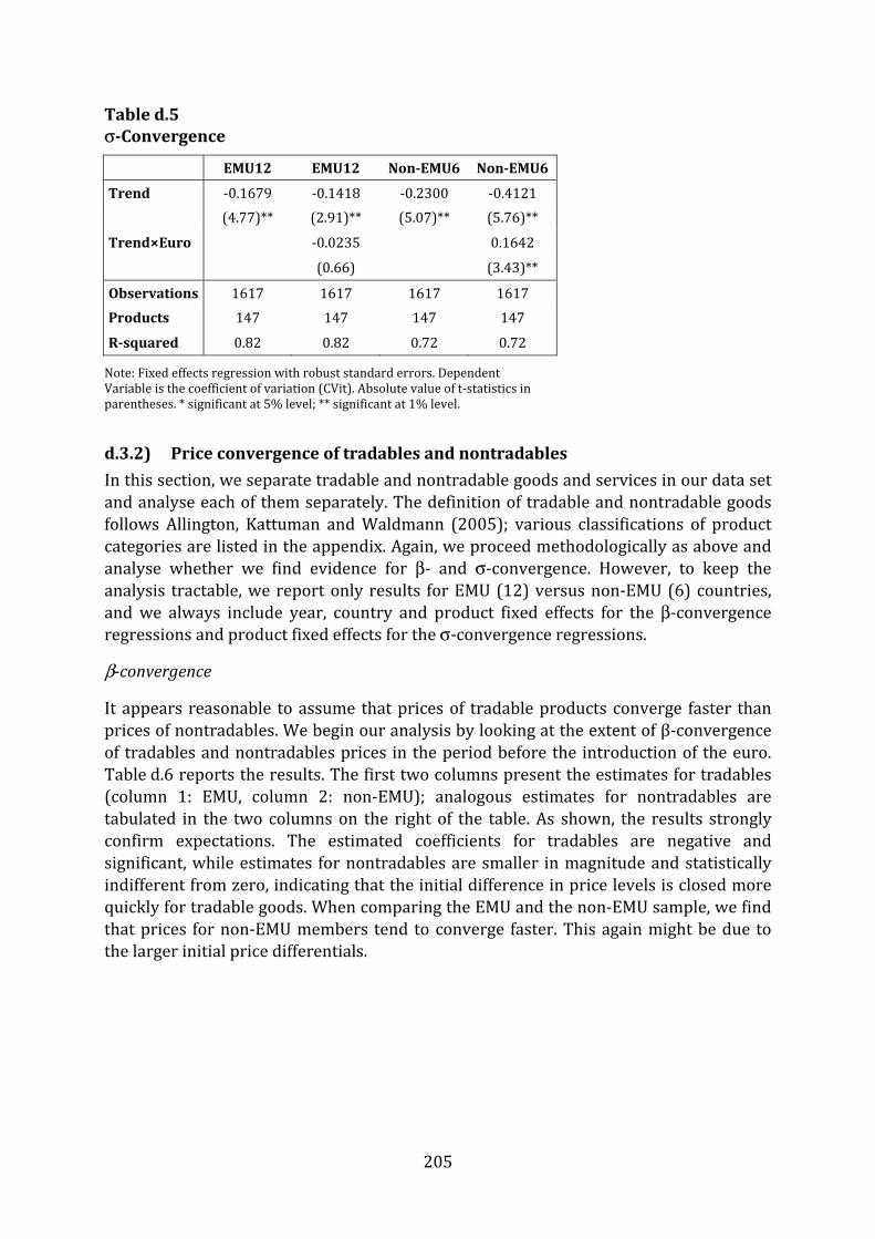
205

Table d.5 σ-Convergence

EMU12 EMU12 Non-EMU6 Non-EMU6

Trend -0.1679 -0.1418 -0.2300 -0.4121 (4.77)** (2.91)** (5.07)** ( 5.76)**Trend×Euro - 0.0235 0.1642 (0.66) (3.43)** Observations 1617 1617 1617 1617 Products 147 147 147 147 R-squared 0.82 0.82 0.72 0.72 Note: Fixed effects regression with robust standard errors. Depeariable is the coefficient of variation (CVit). Absolute value of t-arentheses. * significant at 5% level; ** significant at 1% level. ndent statistics in Vp

d.3.2) Price convergence of tradables and nontradables In this section, we separate tradable and nontradable goods and services in our data set and analyse each of them separately. The definition of tradable and nontradable goods follows Allington, Kattuman and Waldmann (2005); various classifications of product categories are listed in the appendix. Again, we proceed methodologically as above and analyse whether we find evidence for β- and σ-convergence. However, to keep the analysis tractable, we report only results for EMU (12) versus non-EMU (6) countries, and we always include year, country and product fixed effects for the β-convergence regressions and product fixed effects for the σ-convergence regressions. β-convergence It appears reasonable to assume that prices of tradable products converge faster than prices of nontradables. We begin our analysis by looking at the extent of β-convergence of tradables and nontradables prices in the period before the introduction of the euro. Table d.6 reports the results. The first two columns present the estimates for tradables (column 1: EMU, column 2: non-EMU); analogous estimates for nontradables are tabulated in the two columns on the right of the table. As shown, the results strongly confirm expectations. The estimated coefficients for tradables are negative and significant, while estimates for nontradables are smaller in magnitude and statistically indifferent from zero, indicating that the initial difference in price levels is closed more quickly for tradable goods. When comparing the EMU and the non-EMU sample, we find that prices for non-EMU members tend to converge faster. This again might be due to the larger initial price differentials.

206

Table d.6 β-Convergence, 1995–1999

Tradable Nontradable

EMU12 Non-EMU EMU NonEMU

Initial price level, 1995 -0.0413 -0.0735 - 0.0107 - 0.0041 (5.52)** (6.26)** (0.69) (0 ) .21Country Fixed Effects Yes Yes Yes Yes Product Fixed Effects Yes Yes Yes Yes Year Fixed Effects Yes Yes Yes Yes Observations 5460 2730 2280 1140 R-squared 0.28 0.23 0.49 0.54 Np ote: Pooled OLS regression with robust standard errors. Dependent variable is the first difference of the comparative rice level (ΔPij). Absolute value of t-statistics in parentheses. * significant at 5% level; ** significant at 1% level. We redo the estimation above also for the period after the euro cash changeover. Results are reported in Table d.7. Our results suggest that the speed of convergence has increased for EMU member countries; the absolute value of the coefficient for tradables has increased from 0.04 to 0.08. Interestingly, this is not the case for the non-EMU members. This result suggests that indeed the euro might have had a small effect on price convergence, increasing the speed of convergence in tradables. When looking at nontradable goods only (columns 3 and 4) we find that the speed of convergence of nontradables has also increased after the introduction of the euro. This, however, is also true for non-EMU countries. The size of the coefficients indicates that the speed of convergence in nontradable goods prices is significantly higher for EMU countries than for non-EMU countries. Table d.7 β-Convergence, 2001–2005

Tradable Nontradable

EMU N onEMU EMU N onEMU

Initial price level, 2001 -0.0787 -0.0686 -0.0931 -0.0558 (13.20)** (5.59)** (7.75)** (3.54)**

Country Fixed Effects Yes Yes Yes Yes Product Fixed Effects Yes Yes Yes Yes Year Fixed Effects Yes Yes Yes Yes Observations 5460 2730 2280 1140 R-squared 0.06 0.10 0.05 0.14 Np ote: Pooled OLS regression with robust standard errors. Dependent variable is the first difference of the comparative rice level (ΔPij). Absolute value of t-statistics in parentheses. * significant at 5% level; ** significant at 1% level.

207

σ-convergence In this section, we extend our analysis of σ-convergence, allowing for differences across tradable and nontradable goods. As before, we employ the tradability definition of Allington, Kattuman and Waldmann (2005). We compute the coefficients of variation for each country and year for tradable goods prices and nontradable goods prices. We then proceed as above regressing the coefficients of variation on a time trend and the interaction of the time trend with a dummy variable that is equal to 1 after 2002 and zero otherwise. In Table d.8, we report the estimates for the tradable goods. For the EMU sample we can confirm a significant reduction of price dispersion for tradable goods during the period 1995–2005. Again, there is no change in the pace of σ-convergence after the introduction of the euro coins and notes. For the non-EMU countries, the downward trend becomes significant when controlling for the 2002–2005 period. It has about the same size as the coefficient for the EMU. Thus, we cannot find a significant effect of the euro introduction for tradable goods. Table d.8 σ-Convergence, Tradable goods.

EMU EMU Non-EMU Non-EMU

Trend -0.1835 - 0.1021 - 0.0678 -0.1808 (4.98)** (1.72) (1.32) (2.22)*

Trend×Euro - 0.0734 0.1019 (1.82) (1.86)

Observations 1001 1001 1001 1001 Number of products 91 91 91 91 R-squared 0.82 0.82 0.73 0.73 Note: Fixed effects regression with robust standard errors. Dependent Variable is he coefficient of variation (CVit). Absolute value of t-statistics in parentheses. significant at 5% level; ** significant at 1% level. t* In Table d.9, we report the estimates for the nontradable goods. In the first column, we report the coefficient of the trend variable for the whole sample period. Interestingly, we find mild evidence of σ-convergence for the EMU countries. The coefficient on the trend variable is negative and becomes statistically significant, once we control for price changes after the introduction of the euro. The coefficient on the interaction term is positive but insignificant. In columns 3 and 4, we report the estimates for the non-EMU countries. We find a significant downward trend in price dispersion over the period from 1995 to 2005. The pace of convergence has significantly decreased in the period 2002–2005, as indicated by the positive and significant coefficient on the interaction term.

208

Thus, price convergence in nontradable goods is present in EMU countries; the pace of convergence is not significantly different in the period 2002–2005 from the period 1995–2001. When comparing this result to the result from non-EMU member countries, their pace of σ-convergence has slowed down significantly after 2002. Table d.9 σ-Convergence, Non-tradable goods.

EMU EMU Non-EMU Non-EMU

Trend - 0.1247 -0.2536 -0.3392 -0.6647 (1.25) (2.16)* (3.25)** ( 3.98)**

Trend×Euro 0.1163 0.2935 ( 1.23) (2.55)*

Observations 418 418 418 418 Number of products 38 38 38 38 R-squared 0.61 0.62 0.64 0.65 Note: Fixed effects regression with robust standard errors. Dependent Variable is he coefficient of variation (CVit). Absolute value of t-statistics in parentheses. significant at 5% level; ** significant at 1% level. t*

d.3.3) Price convergence of 4 product classifications To further explore the role of tradability for price convergence, we look at four product classifications separately: ‘food: perishable’ (fp), ‘food: nonperishable’ (fn), ‘alcohol and tobacco’ (at), and ‘electrical appliances’ (ea). These product groups can be expected to differ by tradability. For instance, perishable food is assumed to be less tradable than non-perishable food. Similarly, electrical appliances are easily tradable, while alcohol and tobacco, though easily tradable, are marked by high national excise taxes ; see Allington, Kattuman and Waldmann (2005) for a more detailed description. β-convergence We estimate β-convergence – separately for the EMU (12) and non-EMU (6) countries – for the period after the launch of the euro, as this is our main period of interest. In Panel A in Table d.10, we report the results for the EMU countries. Only the product classification ‘perishable food’ shows significant price convergence. In Panel B, we report the estimates for the non-EMU countries. Here, we find evidence that the categories ‘alcohol and tobacco’ and ‘nonperishable food’ converge significantly.

209

Table d.10 001–2005 β-Convergence, 2A: EMU Countries

AT EA FN FP

Initial price level, 2001 0.0126 - 0.0391 0.0015 -0.0156 (1.32) ( 1.52) ( 0.14) ( 1.96)*

Observations 480 720 840 2880 R-squared 0.24 0.08 0.18 0.31 Note: Pooled OLS regression with robust standard errors. Dependent variable is he first difference of the comparative price level (ΔPij). Absolute value of -statistics in parentheses. * significant at 5% level; ** significant at 1% level. tt B: Non-EMU Countries AT EA FN FP

Initial price level, 2001 -0.0743 - 0.0809 -0.07 - 0.0103 (2.34)* (1.24) (2.60)** (0.49)

Observations 240 360 420 1440 R-squared 0.29 0.15 0.2 0.22 Note: Pooled OLS regression with robust standard errors. Dependent variable is he first difference of the comparative price level (ΔPij). Absolute value of -statistics in parentheses. * significant at 5% level; ** significant at 1% level. tt

σ-convergence In Table d.11, we report the corresponding estimates for σ-convergence for the four product categories. In Panel A, we report estimates for the EMU countries. Although there is a significant downward trend for ‘electrical appliances’, there is no evidence that the reduction of price dispersion has changed in the aftermath of the euro introduction. For the control group of non-EMU members, the estimates in Panel B show a similar picture. Here, we find a significant reduction over time in the categories ‘food: perishable’ and ‘alcohol and tobacco’ over the period 1995–2005.

210

Table d.11 σ-Convergence A: EMU Countries AT EA FN FP

Trend - 0.1257 - 0.0994 -0.1991 -0.2841 0.548 0.5929 0.1034 0.0853 (0.55) (0.27) (2.76)** (2.20)* (4.61)** (3.37)** (1.55) (0.81) Trend×Euro - 0.0236 0.0766 - 0.0405 0.0163 (0.11) (0.96) (0.34) (0.24) Observations 44 4 4 66 6 6 77 7 7 264 264 Number of products 4 4 6 6 7 7 24 24 R-squared 0.68 0.68 0.39 0.4 0.84 0.84 0.74 0.74 NAote: Fixed effects regression with robust standard errors. Dependent Variable is the coefficient of variation (CVit). bsolute value of t-statistics in parentheses. * significant at 5% level; ** significant at 1% level. B: Non-EMU Countries AT EA FN FP

Trend 0.8661 1.1311 0.1531 - 0.1075 0.2325 0.4254 -0.226 -0.3709 (4.64)** (5.58)** (1.34) (0.66) (1.14) (1.24) (2.26)* (2.29)* Trend×Euro - 0.2389 0.235 -0.174 0.1307 (1.25) (1.92) (0.75) (1.28) Observations 4 4 44 6 6 66 7 7 77 264 264 Number of products 4 4 6 6 7 7 24 24 R-squared 0.76 0.78 0.43 0.46 0.49 0.49 0.63 0.63 Note: Fixed effects regression with robust standard errors. Dependent Variable is the coefficient of variation (CVit). Absolute value of t-statistics in parentheses. * significant at 5% level; ** significant at 1% level.

211

d.3.4) Price convergence by category In this section, we distinguish the price data by the 12 main product categories. β-convergence In Table d.12, we report the estimates for β-convergence in EMU countries (Panel A) and non-EMU countries (Panel B) after the euro introduction. For EMU countries, we find evidence for beta convergence in the categories ‘communication’, ‘housing, water, electricity, gas’ and ‘recreation and culture’. Divergence can be found in the category ‘miscellaneous goods and services’. In the non-EMU countries, we find that the categories ‘alcoholic beverages, tobacco and narcotics’, ‘food and non-alcoholic beverages’ and ‘recreation and culture’ converge significantly. In the category ‘health’, we find price divergence. σ-convergence Looking at σ-convergence for the different product categories (Table d.13), a faster σ-convergence can be found for EMU member countries in ‘education’ and ‘recreation and culture’ after the introduction of euro coins and notes. For the non-EMU countries, we find that quite a lot of categories show evidence of σ-convergence over the whole sample period: ‘education’, ‘food and non-alcoholic beverages’, ‘furnishings’, ‘health’, housing’, ‘recreation and culture’ and ‘restaurants and hotels’. ‘

212

Table d.12 β-Convergence

β-Convergence, EMU, 2001–2005 Alcoholic

beverages, tobacco

and narcot.

Clothing and

f oot wear Com tionmunica Ed nucatio

Food and non-alcoholic

sbeverage

Furnishings, household equipment

and maintain. Health

Housing, water,

electricity, gas and ot

Misc. goods

and services

Recreation and

culture

Restaurantsand

hotels Transport

Initial price level,2001

0.0127 -0.0264 -0.092 0.029 -0.01 -0.0078 0.0172 -0.0326 0.0403 -0.0186 0.0387 0.0131 (1.55) (1.88) (2.14)* (2.95)** (1.64) (0.43) (1.50) (2.62)** (3.43)** (2.55)* (1.87) (1.50) Observations 600 1200 360 300 4075 1920 840 1080 600 2400 480 1920 R-squared 0.3 0.16 0.18 0.89 0.28 0.21 0.65 0.3 0.2 0.27 0.37 0.21 Note: Pooled OLS regression with robust standard errors. Dependent variable is the first difference of the comparative price level (ΔPij). Absolute value of t-statistics in parentheses. * significant at 5% level; ** significant at 1% level. β-Convergence, Non-EMU, 2001–2005

Alcoholic beverages,

tobacco and narcot

Clothing and

f ootwear Com tionmunica E nducatio

Food and non- alcoholic

b s everage

Furnishings, household equipment

and maintain. Health

Housing, water,

electricity,gas and ot

Misc. goods

and s ervices

Recreationand

culture

Restaurants and

hotels T t ranspor

Initial price level,2001

-0.0582 0.0339 0.026 0.0791 -0.0304 0.0389 0.0524 -0.0449 0.1492 -0.0627 0.0083 0.0229 (2.24)* (1.21) (0.40) (2.77)** (1.96)* (1.49) (2.47)* (1.94) (4.47)** (3.20)** (0.21) (1.15) Observations 300 600 180 300 2040 960 420 660 660 1320 240 1080 R-squared 0.29 0.24 0.18 0.93 0.2 0.25 0.57 0.32 0.36 0.21 0.29 0.23 Note: Pooled OLS regression with robust standard errors. Dependent variable is the first difference of the comparative price level (ΔPij). Absolute value of t-statistics in parentheses. * significant at 5% level; ** significant at 1% level.

213

Table d.13 σ-Convergence

σ-Convergence, EMU Alcoholic beverages,

tobacco and narcot.

Alcoholic beverages,

tobacco and narcot.

Clothing and

footwear

Clothing and

f ootwear Com ion municat Com ation munic E ducation E ducation

Food and non-

alcoholic b s everage

Food and non-

alcoholic b s everage

Trend -0.1198 -0.1123 -0.4846 -0.5215 -1.6676 -1.82 -0.6108 -0.3135 0.1728 0.1405 (0.75) (0.38) (6.28)** (3.54)** (5.49)** (4.06)** (10.71)** (2.22)* (2.96)** (1.55) Trend×Euro -0.0068 0.0333 0.1374 -0.2681 0.0291 -0.04 -0.3 -0.4 (2.81)** -0.5 Observations 55 55 110 110 33 33 55 55 374 374 Number of products 5 5 10 10 3 3 5 5 34 34 R-squared 0.89 0.89 0.88 0.88 0.67 0.67 0.57 0.66 0.75 0.75 Furnishings,

household equipment

and ma

Furnishings, household equipment

and ma Health Health

Housing, water,

electricity, gas and ot

Housing, water,

electricity, gas and ot

Miscellaneous goods and

services

Miscellaneous goods and

services Recreation and culture

Recreation and culture

Trend 0.0345 0.0637 -0.7586 -0.6925 -0.1014 0.1792 -0.2491 -0.3288 -0.3253 -0.1323 (0.31) (0.54) (4.46)** (2.95)** (0.67) (0.81) (3.10)** (2.36)* (4.93)** (1.11) Trend×Euro -0.0263 -0.0596 -0.253 0.0719 -0.174 -0.23 -0.36 -1.64 -0.67 (2.17)* Observations 374 176 176 77 77 121 121 121 242 242 Number of products 34 16 16 7 7 11 11 11 22 22 R-squared 0.75 0.83 0.83 0.69 0.69 0.7 0.7 0.93 0.82 0.82

Restaurants a s nd hotel

Restaurants a s nd hotel Transport Transport

Trend -0.7942 -0.641 0.1051 -0.1039 (2.88)** (1.56) (0.76) (0.73) Trend×Euro -0.1381 0.1885 -0.55 -1.48 Observations 242 242 44 44 Number of products 22 22 4 4 R-squared 0.82 0.83 0.64 0.65

214

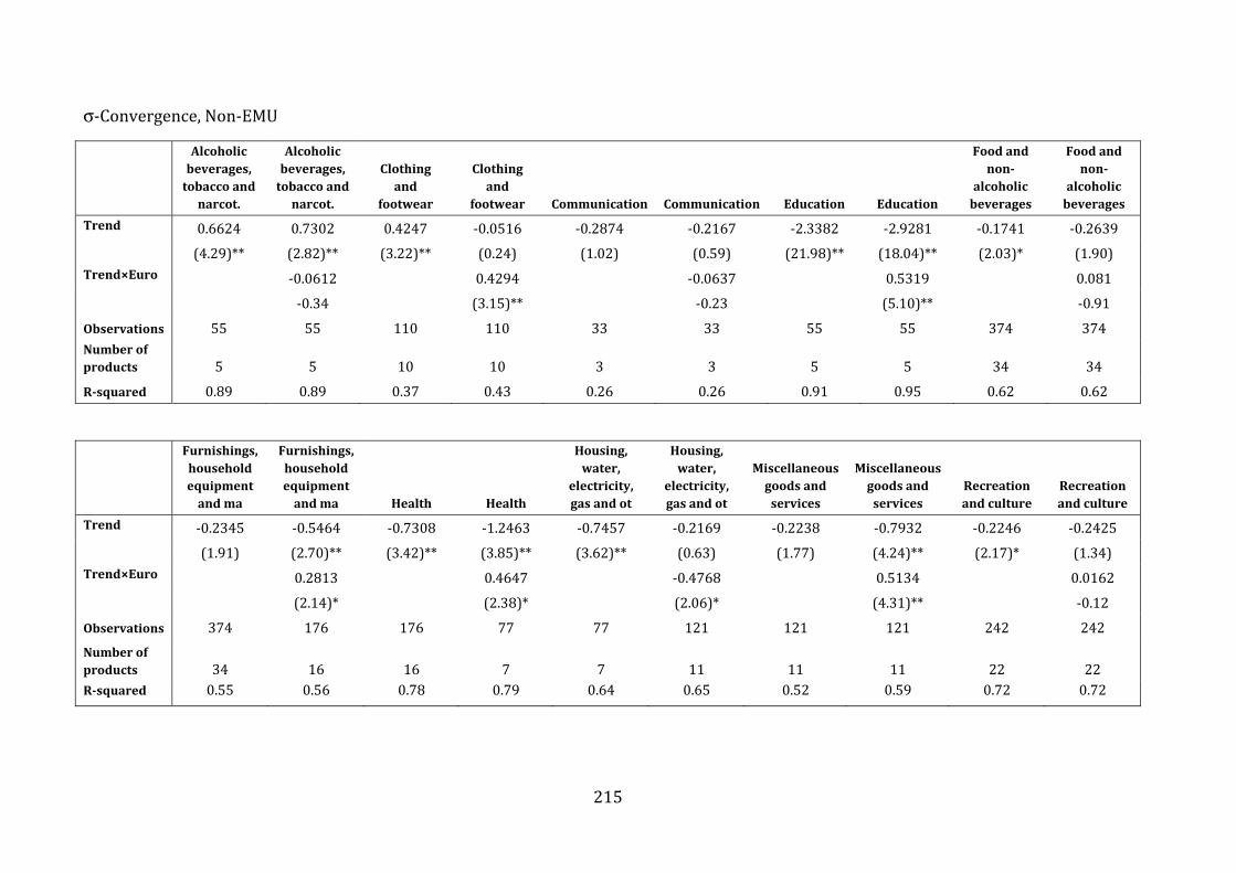
215

σ-Convergence, Non-EMU Alcoholic beverages,

tobacco and narcot.

Alcoholic beverages,

tobacco and narcot.

Clothing and

f ootwear

Clothing and

f ootwear Com ion municat Com ion municat E ducation E ducation

Food and non-

alcoholic b s everage

Food and non-

alcoholic b everages

Trend 0.6624 0.7302 0.4247 -0.0516 -0.2874 -0.2167 -2.3382 -2.9281 -0.1741 -0.2639 (4.29)** (2.82)** (3.22)** (0.24) (1.02) (0.59) (21.98)** (18.04)** (2.03)* (1.90) Trend×Euro -0.0612 0.4294 -0.0637 0.5319 0.081 -0.34 (3.15)** -0.23 (5.10)** -0.91 Observations 55 55 110 110 33 33 55 55 374 374 Number of products 5 5 10 10 3 3 5 5 34 34 R-squared 0.89 0.89 0.37 0.43 0.26 0.26 0.91 0.95 0.62 0.62 Furnishings,

household equipment

and ma

Furnishings, household equipment

and ma Health Health

Housing, water,

electricity, gas and ot

Housing, water,

electricity, gas and ot

Miscellaneous goods and

services

Miscellaneous goods and

services Recreation and culture

Recreation and culture

Trend -0.2345 -0.5464 -0.7308 -1.2463 -0.7457 -0.2169 -0.2238 -0.7932 -0.2246 -0.2425 (1.91) (2.70)** (3.42)** (3.85)** (3.62)** (0.63) (1.77) (4.24)** (2.17)* (1.34) Trend×Euro 0.2813 0.4647 -0.4768 0.5134 0.0162 (2.14)* (2.38)* (2.06)* (4.31)** -0.12 Observations 374 176 176 77 77 121 121 121 242 242 Number of products 34 16 16 7 7 11 11 11 22 22 R-squared 0.55 0.56 0.78 0.79 0.64 0.65 0.52 0.59 0.72 0.72

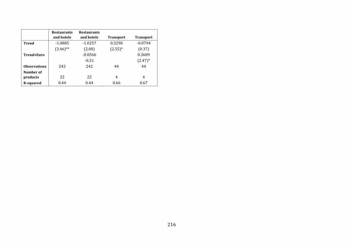
216

Restaurants a s nd hotel

Restaurants a nd hotels Transport Transport

Trend -1.0885 -1.0257 0.3298 -0.0794 (3.46)** (2.00) (2.55)* (0.37) Trend×Euro -0.0566 0.3689 -0.21 (2.47)* Observations 242 242 44 44 Number of products 22 22 4 4 R-squared 0.44 0.44 0.66 0.67

217

d.3.5) Price convergence by product In this section, we present the results for β-convergence for individual product groups. We report only those coefficients that are significant and show convergence after the euro cash changeover. We find evidence for σ- and β-convergence only for two product groups: ‘lamb, mutton and goat’ and ‘jewellery, clocks and watches’. Evidence of β-convergence can be found for the product groups ‘fresh milk’, ‘tobacco’, ‘bedroom furniture’, ‘small electric household appliances’, ‘domestic services (non-tradable)’ and ‘motor cars with petrol engine of cubic capacity of less than 1200cc’. β-convergence

Table d.14 β-Convergence

β-Convergence, EMU, 2001–2005 Product group Initial price level, 2001 Obse ions rvat R-squared 1101123 -0.0776 (2.05)* 120 0.03 1112311 -0.0923 (2.18)* 120 0.04 1105112 -0.0395 (2.23)* 120 0.04 1107112 -0.0836 (2.43)* 120 0.05 1102211 -0.0813 (2.44)* 120 0.05 1101141 -0.1221 (2.49)* 120 0.05 1105621 -0.0727 (2.70)** 120 0.06 1105321 -0.0968 (3.07)** 120 0.07 Note: Pooled OLS regression with robust standard errors. Dependent variable is the first difference of the comparative price level (ΔPij). Absolute value of t-statistics in parentheses. * significant at 5% level; ** significant at 1% level.

β-Convergence, EMU, 2001–2005 Product group Initial price level, 2001 Observations R-squared 1104411 -0.178 (3.22)** 60 0.15 Note: Pooled OLS regression with robust standard errors. Dependent variable is the first difference of the comparative price level (ΔPij). Absolute value of t-statistics in parentheses. * significant at 5% level; ** significant at 1% level.

218

σ-convergence

Table d.15 σ-Convergence after euro introduction

σ-Convergence after euro introduction, EMU Product

group Trend Trend×Euro Observations R-squared 1105611 -0.0021 (2.17) -0.0019 (2.73)* 11 0.87 1101115 0.0027 (0.98) -0.0046 (2.35)* 11 0.48 1103123 -0.0036 (1.44) -0.0068 (3.89)** 11 0.89 1109511 0.0067 (1.83) -0.0119 (4.57)** 11 0.78 1101123 0.0041 (2.02) -0.0128 (8.84)** 11 0.95 1111112 0.0097 (2.13) -0.0158 (4.88)** 11 0.8 1112311 0.0165 (2.70)* -0.0163 (3.76)** 11 0.64 1104111 0.0149 (3.85)** -0.0173 (6.32)** 11 0.84 1101112 0.0141 (6.31)** -0.0190 (12.00)** 11 0.95 NA ote: Fixed effects regression with robust standard errors. Dependent Variable is the coefficient of variation (CVit). bsolute value of t-statistics in parentheses. * significant at 5% level; ** significant at 1% level.

σ-Convergence after euro introduction, Non-EMU Product

group Trend Trend×Euro Obser ions vat R-squared 1103123 0.0330 (3.61)** -0.0406 (6.28)** 11 0.85 1105511 0.0139 (3.25)* -0.0188 (6.21)** 11 0.85 1103212 0.0035 (0.76) -0.0093 (2.87)* 11 0.64 1103111 0.0051 (1.47) -0.0061 (2.46)* 11 0.45 NA ote: Fixed effects regression with robust standard errors. Dependent Variable is the coefficient of variation (CVit). bsolute value of t-statistics in parentheses. * significant at 5% level; ** significant at 1% level.

d.4) Determinants of the Speed of Convergence For the empirical analysis of the evolution of price convergence and its determinants, we essentially follow Bergin and Glick (2007). In order to identify the effect of the euro, we (aim to) control for all other possible determinants of bilateral price differences. In practice, we experiment with a wide range of potential variables, including, for instance, language barriers, and also more unconventional measures such as union density (possibly affecting wages). Our benchmark specification is given by the following quatione 31: ijt

ttt

jjj

iiiijj

tradablei

tradable

jiijijijijijt

yearcountrycountryexrww

ulculceuroEMUEUEMUdistMSE

ελββαα

αααααα

+++++−+

−+×++++=

∑∑∑76

543210 )ln( where untries, • i and j denote co • t denotes time • MSEijt is the mean squared error; the measure of price dispersion between country i and j in year t • ln(dis , t ij) is the log of the distance between the capitals of countries i and j, • EMUij is a dummy that is equal to one if both countries are member of the European Monetary Union, • EUij is a dummy that is equal to one if both countries are member of the EU, • EMUij×euro is an interaction term that interacts the variable EMU with a binary variable that is equal to unity for the years after the Euro introduction and zero otherwise, • ulci denotes the unit labor cost in country i , • wtr ption basket, adable is the weight of tradable goods in country i’s consum • exr is th darde stan deviation of the monthly exchange rate, • cou comprehensive set of country and year dummies and ntryi and yeart are a • εijt is an iid error term. We include the absolute difference in unit labor costs to capture supply side effects on price levels. The weight of tradables is included to capture differences in the onsumption basket in different countries. We would expect that countries with a c 219 31 For another approach to identify determinants of price dispersion, see Crucini, Telmer and Zachariadis (2005) or Beck and Weber (2003).

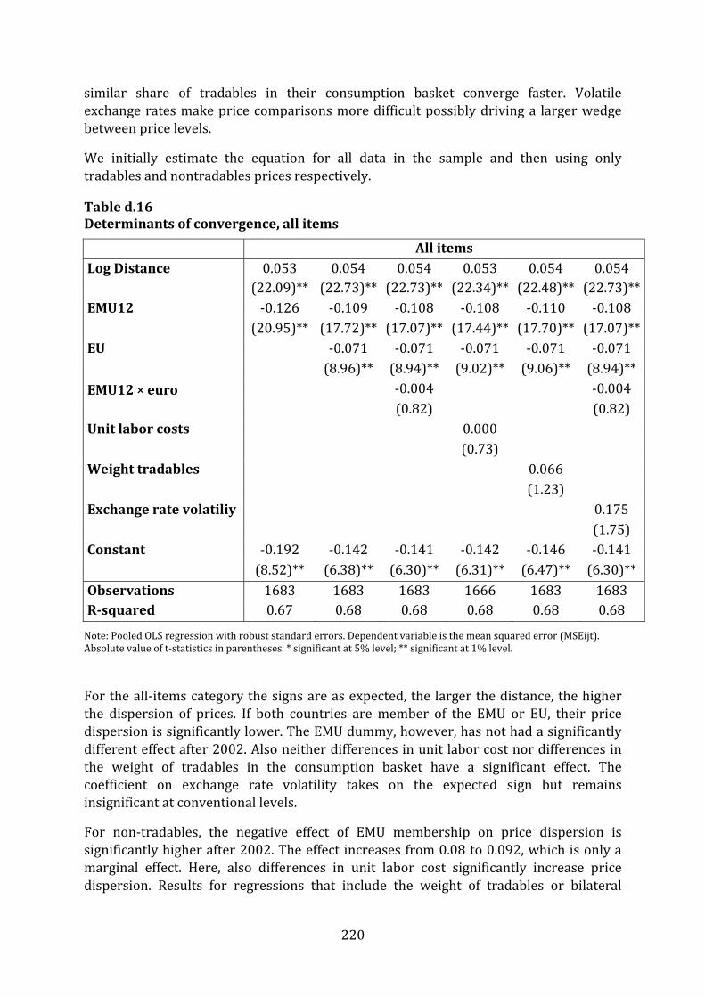
220

similar share of tradables in their consumption basket converge faster. Volatile exchange rates make price comparisons more difficult possibly driving a larger wedge between price levels. We initially estimate the equation for all data in the sample and then using only tradables and nontradables prices respectively. Table d.16 Determinants of convergence, all items

All items Log Distance 0.053 0.054 0.054 0.053 0.054 0.054 (22.09)** (22.73)** (22.73)** (22.34)** (22.48)** (22.73)**EMU12 -0.126 -0.109 -0.108 -0.108 -0.110 -0.108 (20.95)** (17.72)** (17.07)** (17.44)** (17.70)** (17.07)**EU -0.071 -0.071 -0.071 -0.071 -0.071 (8.96)** (8.94)** (9.02)** (9.06)** ( 8.94)**EMU12 × euro -0.004 -0.004 (0.82) (0.82) Unit labor costs 0.000 (0.73) Weight tradables 0.066 (1.23) Exchange rate volatiliy 0.175 (1.75) Constant -0.192 -0.142 -0.141 -0.142 -0.146 -0.141 (8.52)** (6.38)** (6.30)** (6.31)** (6.47)** (6.30)** Observations 1683 1683 1683 1666 1683 1683 R-squared 0.67 0.68 0.68 0.68 0.68 0.68 NAote: Pooled OLS regression with robust standard errors. Dependent variable is the mean squared error (MSEijt). bsolute value of t-statistics in parentheses. * significant at 5% level; ** significant at 1% level. For the all-items category the signs are as expected, the larger the distance, the higher the dispersion of prices. If both countries are member of the EMU or EU, their price dispersion is significantly lower. The EMU dummy, however, has not had a significantly different effect after 2002. Also neither differences in unit labor cost nor differences in the weight of tradables in the consumption basket have a significant effect. The coefficient on exchange rate volatility takes on the expected sign but remains einsignificant at conv ntional levels. For non-tradables, the negative effect of EMU membership on price dispersion is significantly higher after 2002. The effect increases from 0.08 to 0.092, which is only a marginal effect. Here, also differences in unit labor cost significantly increase price dispersion. Results for regressions that include the weight of tradables or bilateral

221

exchange rate volatility as control variables yield insignificant results and, therefore, are unreported. For tradables, our results show that especially the EU membership dummy has a larger effect on price dispersion compared to non-tradable prices. A similarly counterintuitive result is observed for distance; the distance effect on prices is higher for tradables than for nontradables, perhaps questioning the quality of the underlying data. Table d.17 Determinants of convergence, by tradability

Non-Tradables Tradables Log Distance 0.038 0.038 0.038 0.037 0.045 0.047 0.047 0.047 (15.94)** (16.15)** (16.15)** (15.63)** (23.85)** (25.06)** (25.06)** (24.92)**EMU12 -0.090 -0.084 -0.080 -0.082 -0.108 -0.088 -0.090 -0.087 (16.03)** (14.55)** (13.66)** (14.46)** (20.10)** (16.69)** (16.55)** (16.36)**EU -0.028 -0.028 -0.028 -0.084 -0.084 -0.084 (2.86)** ( 2.83)** (2.85)** (9.68)** (9.64)** (9.67)** EMU12 × euro -0.012 0.006 (2.57)* (1.75) Unit labor c. 0.001 -0.001 (2.44)* (1.63) Constant -0.116 -0.097 -0.093 -0.096 -0.186 -0.128 -0.130 -0.128 (5.34)** (4.24)** (4.06)** (4.15)** (10.59)** (7.17)** (7.31)** (7.17)** Observations 1683 1683 1683 1666 1683 1683 1683 1666 R-squared 0.63 0.63 0.63 0.63 0.69 0.71 0.71 0.71 NA ote: Pooled OLS regression with robust standard errors. Dependent variable is the mean squared error (MSEijt). bsolute value of t-statistics in parentheses. * significant at 5% level; ** significant at 1% level.

222

References Allington, Nigel F.B., Kattuman, Paul A. and Waldmann, Florian A. (2005): One Market, One Money, One Price?, International Journal of Central Banking, 1, December: 73–115. Baldwin, Richard, (2006): In or Out: Does It Make a Difference? London, Centre for Economic Policy Research. Baye, Michael R., Gatti, J. Rupert J., Kattuman, Paul A. and Morgan, John. (2006): Did the Euro Foster Online Price Competition? Evidence from an International Price Comparison Site, Economic Inquiry, 44, April: 265–279. Beck, Guenter W. and Weber, Axel A. (2003): How Wide are European Borders? On the Integration Effects of Monetary Unions, Goethe University Frankfurt and Deutsche Bundesbank. Bergin, Paul R. and Glick, Reuven (2007): Global Price Dispersion: Are Prices Converging or Diverging?, Journal of International Money and Finance, 26, September: 703–729. Chen, Lein-Lein, Choi, Seungmook and Devereux, John (2008): Have Absolute Price Levels Converged for Developed Economies? The Evidence Since 1870, 90, February: 29–36. Crucini, Mario J., Telmer, Chris I. and Zachariadis, Marios (2005): Price Dispersion: The Role of Borders, Distance and Location, Vanderbilt University, Carnegie Mellon University, Louisiana State University. Dreger, Christian, Kholodilin, Konstantin, Lommatzsch, Kirsten, Slacalek, Jirka and Wozniak, Przemyslaw (2007): Price Convergence in the Enlarged Internal Market, European Economy Economic Papers 292. Engel, Charles and Rogers, John H. (1996): How Wide is the Border?, American Economic Review, 86, December: 1112–1125. Engel, Charles and Rogers, John H. (2004): European Product Market Integration After the Euro, Economic Policy, July: 347–384. Foad, Hisham S. (2007): Europe Without Borders? The Effect of the Euro on Price Convergence, San Diego State University. Friberg, Richard and Mathä, Thomas Y. (2004): Does a Common Currency Lead to (More) Price Equalization? The Role of Psychological Pricing Points, Economics Letters, 84, August: 281–287. Gil-Pareja, Salvador and Sosvilla-Rivero, Simón (2008): Price Convergence in the European Car Market, Applied Economics, 40, 2: 241–250. Goldberg, Pinelopi K. and Verboven, Frank (2004): Cross-Country Price Dispersion in the Euro Area: A Case Study of the European Car Market, Economic Policy, October: 483–521.

223

Goldberg, Pinelopi K. and Verboven, Frank (2005): Market Integration and Convergence to the Law of One Price: Evidence from the European Car Market, Journal of International Economics, 65, January: 49–73. Imbs, Jean, Mumtaz, Haroon, Ravn, Morton O. and Rey, Hélène (2004): Price Convergence: What’s on TV?, London Business School and Princeton University. Isgut, Alberto E. (2004): Common Currencies and Market Integration across Cities: How Strong is the Link?, in Volbert Alexander, Jacques Mélitz, and George M. von Furstenberg (eds.), Monetary Unions and Hard Pegs: Effects on Trade, Financial Development, and Stability, Oxford, Oxford University Press. Lein, Sarah M. and Volker Nitsch (2008): Pasta, Pets and Prostitution: The Euro’s Effect on Prices, ETH Zurich and Swiss National Bank. Lutz, Matthias (2003): Price Convergence under EMU? First Estimates, Universität St. Gallen Discussion Paper 2003–08. Mathä, Thomas Y. (2003): What to Expect of the Euro? Analysing Price Differences of Individual Products in Luxembourg and its Surrounding Regions, Banque Centrale du Luxembourg Working Paper 8. Mathä, Thomas Y. (2005): Der Euro und Weiterführende Regionale Preiskonvergenz? Resultate aus der ‚Groß-Region’ um Luxemburg, Perspektiven der Wirtschaftspolitik, 6, February: 57–70. Parsley, David C. and Wei, Shang-Jin (2001): Limiting Currency Volatility to Stimulate aper #8468. Goods Market Integration: A Price Based Approach, NBER Working PParsley, David C. and Wei, Shang-Jin (2007): A Prism into the PPP Puzzles: The Micro-Foundations of Big Mac Real Exchange Rates, Economic Journal, 117, October: 1336–1356. Parsley, David C. and Wei, Shang-Jin (2008): In Search of a Euro Effect: Big Lessons from a Big Mac Meal?, Journal of International Money and Finance, forthcoming. Rogers, John H. (2007): Monetary Union, Price Level Convergence, and Inflation: How 96. Close is Europe to the USA?, Journal of Monetary Economics, 50, April: 785–7Rogoff, Kenneth (1996): The Purchasing Power Parity Puzzle, Journal of Economic Literature, 34, June: 647–668. Sosvilla-Rivero, Simón and Gil-Pareja, Salvador (2004): Price Convergence in the European Union, Applied Economics Letters, 11, 1: 39–47. Wolszczak-Derlacz, Joanna (2006): One Europe, One Product, Two Prices: The Price Disparity in the EU, Gdańsk University of Technology.

Appendix

Product groups

Table d.A.1

product-number productname akw category p-group 1101111 Rice 1 Food and non-alcoholic beverages 1101112 Other cereals, flour and other cereal products 1 Food and non-alcoholic beverages 1101113 Bread 1 Food and non-alcoholic beverages fp 1101114 Other bakery products 1 Food and non-alcoholic beverages fp 1101115 Pasta products 1 Food and non-alcoholic beverages fp 1101121 Beef and Veal 1 Food and non-alcoholic beverages fp 1101122 Pork 1 Food and non-alcoholic beverages fp 1101123 Lamb, mutton and goat 1 Food and non-alcoholic beverages fp 1101124 Poultry 1 Food and non-alcoholic beverages fp 1101125 Other meats and edible offal 1 Food and non-alcoholic beverages fp 1101126 Delicatessen and other meat preparations 1 Food and non-alcoholic beverages fp 1101131 Fresh, chilled or frozen fish and seafood 1 Food and non-alcoholic beverages fp 1101132 Preserved or processed fish and seafood 1 Food and non-alcoholic beverages fp 1101141 Fresh milk 1 Food and non-alcoholic beverages fp 1101142 Preserved milk and other milk products 1 Food and non-alcoholic beverages fp 1101143 Cheese 1 Food and non-alcoholic beverages fp 1101144 Eggs and egg-based products 1 Food and non-alcoholic beverages fp 1101151 Butter 1 Food and non-alcoholic beverages fp 1101152 Margarine 1 Food and non-alcoholic beverages fp 1101153 Other edible oils and fats 1 Food and non-alcoholic beverages fp 1101161 Fresh or chilled fruit 1 Food and non-alcoholic beverages fp

2241101162 Frozen, preserved or processed fruit and fruit-based products 1 Food and non-alcoholic beverages fp

product-number productname akw category p-group 1101171 Fresh or chilled vegetables other than potatoes 1 Food and non-alcoholic beverages fp 1101172 Fresh or chilled potatoes 1 Food and non-alcoholic beverages fp 1101173 Frozen, preserved or processed vegetables and vegetable-based 1 Food and non-alcoholic beverages fp 1101181 Sugar 1 Food and non-alcoholic beverages fn 1101182 Jams, marmalades and honey 1 Food and non-alcoholic beverages Fn 1101183 Confectionery, chocolate and other cocoa preparations 1 Food and non-alcoholic beverages fn 1101184 Edible ice, ice cream and sorbet 1 Food and non-alcoholic beverages fp 1101191 Food products n.e.c. 1 Food and non-alcoholic beverages 1101211 Coffee, tea and cocoa 1 Food and non-alcoholic beverages fn 1101221 Mineral waters 1 Food and non-alcoholic beverages fn 1101222 Soft drinks and concentrates 1 Food and non-alcoholic beverages fn 1101223 Fruit and vegetable juices 1 Food and non-alcoholic beverages fn 1102111 Spirits 1 Alcoholic beverages, tobacco and narcotics at 1102121 Wine 1 Alcoholic beverages, tobacco and narcotics at 1102131 Beer 1 Alcoholic beverages, tobacco and narcotics at 1102211 Tobacco 1 Alcoholic beverages, tobacco and narcotics at 1102311 Narcotics 1 Alcoholic beverages, tobacco and narcotics 1103111 Clothing materials 1 Clothing and footwear 1103121 Men's clothing 1 Clothing and footwear 1103122 Women's clothing 1 Clothing and footwear 1103123 Children’s and infant’s clothing 1 Clothing and footwear 1103131 Other articles of clothing and clothing accessories 1 Clothing and footwear 1103141 Cleaning, repair and hire of clothing 2 Clothing and footwear 1103211 Men's footwear 1 Clothing and footwear 1103212 Women's footwear 1 Clothing and footwear 1103213 Children's and infant's footwear 1 Clothing and footwear 1103221 Repair and hire of footwear 2 Clothing and footwear

2251104111 Actual rentals for housing 2 Housing, water, electricity, gas and other fuels

product-number productname akw category p-group 1104211 Imputed rentals for housing 2 Housing, water, electricity, gas and other fuels 1104311 Materials for the maintenance and repair of the dwelling 1 Housing, water, electricity, gas and other fuels 1104321 Services for the maintenance and repair of the dwelling 2 Housing, water, electricity, gas and other fuels 1104411 Water supply 2 Housing, water, electricity, gas and other fuels 1104421 Miscellaneous services relating to the dwelling Housing, water, electricity, gas and other fuels 1104511 Electricity 2 Housing, water, electricity, gas and other fuels 1104521 Gas 2 Housing, water, electricity, gas and other fuels 1104531 Liquid fuels 1 Housing, water, electricity, gas and other fuels 1104541 Solid fuels 1 Housing, water, electricity, gas and other fuels 1104551 Heat energy Housing, water, electricity, gas and other fuels 1105111 Kitchen furniture 1 Furnishings, household equipment and 1105112 Bedroom furniture 1 Furnishings, household equipment and 1105113 Living-room and dining-room furniture 1 Furnishings, household equipment and 1105114 Other furniture and furnishings 1 Furnishings, household equipment and 1105121 Carpets and other floor coverings 1 Furnishings, household equipment and 1105131 Repair of furniture, furnishings and floor coverings 2 Furnishings, household equipment and 1105211 Household textiles 1 Furnishings, household equipment and 1105311 Major household appliances whether electric or not 1 Furnishings, household equipment and ea 1105321 Small electric household appliances 1 Furnishings, household equipment and ea 1105331 Repair of household appliances 2 Furnishings, household equipment and 1105411 Glassware, tableware and household utensils 1 Furnishings, household equipment and 1105511 Major tools and equipment 1 Furnishings, household equipment and 1105521 Small tools and miscellaneous accessories 1 Furnishings, household equipment and 1105611 Non-durable household goods 1 Furnishings, household equipment and 1105621 Domestic services 2 Furnishings, household equipment and 1105622 Household services 2 Furnishings, household equipment and 1106111 Pharmaceutical products 1 Health

2261106121 Other medical products 1 Health

product-number productname akw category p-group 1106131 Therapeutical appliances and equipment 1 Health 1106211 Medical Services 2 Health 1106221 Services of dentists 2 Health 1106231 Paramedical services 2 Health 1106311 Hospital services 2 Health 1107111 Motor cars with diesel engine 1 Transport 1107112 Motor cars with petrol engine of cubic capacity of less than 1200cc 1 Transport 1107113 Motor cars with petrol engine of cubic capacity of 1200cc to 1699cc 1 Transport 1107114 Motor cars with petrol engine of cubic capacity of 1700cc to 2999cc 1 Transport 1107115 Motor cars with petrol engine of cubic capacity of 3000cc and over 1 Transport 1107121 Motor cycles 1 Transport 1107131 Bicycles 1 Transport 1107141 Animal drawn vehicles Transport 1107211 Spare parts and accessories for personal transport equipment 1 Transport 1107221 Fuels and lubricants for personal transport equipment 1 Transport 1107231 Maintenance and repair of personal transport equipment 2 Transport 1107241 Other services in respect of personal transport equipment 2 Transport 1107311 Passenger transport by railway 2 Transport 1107321 Passenger transport by road 2 Transport 1107331 Passenger transport by air 2 Transport 1107341 Passenger transport by sea and inland waterway 2 Transport 1107351 Combined passenger transport Transport 1107361 Other purchased transport services 2 Transport 1108111 Postal services 2 Communication 1108211 Telephone and telefax equipment 1 Communication ea 1108311 Telephone and telefax services 2 Communication 1109111 Equipment for the reception, recording and reproduction of sound 1 Recreation and culture ea

2271109121 Photographic and cinematographic equipment and optical 1 Recreation and culture ea

product-number productname akw category p-group 1109131 Information processing equipment 1 Recreation and culture ea 1109141 Pre-recorded recording media 1 Recreation and culture 1109142 Unrecorded recording media 1 Recreation and culture 1109151 Repair of audio-visual, photographic and information processing 2 Recreation and culture 1109211 Major durables for outdoor recreation 1 Recreation and culture 1109221 Musical instruments and major durables for indoor recreation 1 Recreation and culture 1109231 Maintenance and repair of other major durables for recreation and 2 Recreation and culture 1109311 Games, toys and hobbies 1 Recreation and culture 1109321 Equipment for sport, camping and open-air recreation 1 Recreation and culture 1109331 Gardens, plants and flowers 1 Recreation and culture 1109341 Pets and related products 1 Recreation and culture 1109351 Veterinary and other services for pets 2 Recreation and culture 1109411 Recreational and sporting services 2 Recreation and culture 1109421 Photographic services 2 Recreation and culture 1109422 Other cultural services 2 Recreation and culture 1109431 Games of chance Recreation and culture 1109511 Books 2 Recreation and culture 1109521 Newspapers and periodicals 2 Recreation and culture 1109531 Miscellaneous printed matter, stationery and drawing materials 1 Recreation and culture 1109611 Package holidays Recreation and culture 1110111 Pre-primary and primary education Education 1110211 Secondary education Education 1110311 Post-secondary education Education 1110411 Tertiary education Education 1110511 Education not definable by level Education 1111111 Restaurant services whatever the type of establishment 2 Restaurants and hotels 1111112 Pubs, bars, cafés, tea rooms and the like 2 Restaurants and hotels

2281111121 Canteens 2 Restaurants and hotels

229

product-number productname akw category p-group 1111211 Accommodation services 2 Restaurants and hotels 1112111 Hairdressing salons and personal grooming establishments 2 Miscellaneous goods and services 1112121 Electric appliances for personal care 1 Miscellaneous goods and services 1112131 Other appliances, articles and products for personal care 1 Miscellaneous goods and services 1112211 Prostitution Miscellaneous goods and services 1112311 Jewellery, clocks and watches 1 Miscellaneous goods and services 1112321 Other personal effects 1 Miscellaneous goods and services 1112411 Social protection Miscellaneous goods and services 1112511 Insurance Miscellaneous goods and services 1112611 FISIM Miscellaneous goods and services 1112621 Other financial services n.e.c. Miscellaneous goods and services 1112711 Other services n.e.c. Miscellaneous goods and services 1113111 Net purchases abroad Net purchases abroad Notes: Product groups with akw>0 are included in Allington, Kattuman and Waldmann (2005). ‘1’ denotes that the product is tradable, ‘2’ denotes classification as nontradable.

230

A differences-in-differences approach While most studies find little effect of the euro on prices, there is one study that reports a positive effect of the common currency on price convergence, Allington, Kattuman and Waldmann (2005). In his comprehensive survey of the literature, Baldwin (2006) argues that this “is the best paper in the field to date, in my opinion”. Since we use a basically similar data set, we aim to replicate their results. Following Allington, Kattuman and Waldmann (2005), we have performed a differences-in-differences analysis of the price effects of the euro. More specifically, we have explored regressions of the form: CVg,p,t = α + β1 ·EMU + β2 ·post01 + β3 ·EMU × post01 + γ1 + γ2 τ × EMU + γ3 τ × post01 +γ4 · τ ×·EMU × post01 + Σk δk Γg,t,k + Σj ηj· Θj + eg,p,t The following tables report the set of results. It turns out that Allington, Kattuman and Waldmann’s (2005) findings are not robust. Our benchmark differences-in-differences specification suggests that price dispersion within EMU is on average significantly lower than for other European countries and has generally fallen after the euro cash changeover. However, dispersion has fallen for the full sample so that no separate effect of euro notes and coins on prices is identifiable. Extending the regression specification by including additional control variables leaves the basic result unaffected, especially since the coefficients on the various treatment effects introduced by Allington, Kattuman and Waldmann (2005) take on different signs. A more detailed discussion of the results is provided in Lein and Nitsch (2008). Table d.A.2 Benchmark DiD (EMU12/EU15 plus 3)

Full Sample Goods & Services ( 12 )

Bench-mark

EMU12 0.001 (0.001) -0.013** (0.001) -0.020** (0.001) Post2001 -0.025** (0.001) -0.010** (0.001) -0 .007**(0.002) EMU12 × Post2001 0.008** (0.001) 0.005** (0.002) 0.001 (0.002) # products 224 147 129 # obs. 44352 29106 25542 Adj. R2 0.64 0.63 0.62

231

Table d.A.3 Does specification matter?

Be k nchmar Ad ls d contro A s dd trend

EMU12 -0.020** (0.001) -0.022** (0.002) - 0.017**(0.004) Post2001 -0.007** (0.002) -0.007** (0.002) -0.002 (0.003) EMU12 × Post2001 0.001 (0.002) 0.014** (0.002) 0.028** (0.006) SD (output growth) 0 .008**(0.001) 0.007** (0.001) SD (inflation) 0.001 (0.001) -0.003 (0.002) SD (exchange rates) 0.003** (0.001) 0.003** (0.001) Trend -0.0007 (0.0006) Trend × EMU12 -0.0009 (0.0008) Trend × EMU12 × Post2001

-0.0015* (0.0007) # products 129 129 129 # obs. 25542 25542 25542 Adj. R2 0.62 0.63 0.63