
CMMSE VOLUME IV
338
Proceedings of the 2012 International Conference on Computational and Mathematical Methods in Science and Engineering Murcia, Spain July 2-5, 2012 CMMSE VOLUME IV Editor: J. Vigo-Aguiar Associate Editors: A.P. Buslaev, A. Cordero, M. Demiralp, I. P. Hamilton, E. Jeannot, V.V. Kozlov, M.T. Monteiro, J.J. Moreno, J.C. Reboredo, P. Schwerdtfeger, N. Stollenwerk, J.R. Torregrosa, E. Venturino, J. Whiteman
-
Upload
khangminh22 -
Category
Documents
-
view
1 -
download
0
Transcript of CMMSE VOLUME IV

Proceedings of the 2012 International Conference on
Computational and Mathematical Methods in Science and Engineering
Murcia, Spain
July 2-5, 2012
CMMSE VOLUME IV
Editor: J. Vigo-Aguiar
Associate Editors: A.P. Buslaev, A. Cordero, M. Demiralp, I. P. Hamilton, E. Jeannot, V.V. Kozlov,
M.T. Monteiro, J.J. Moreno, J.C. Reboredo, P. Schwerdtfeger, N. Stollenwerk, J.R. Torregrosa,
E. Venturino, J. Whiteman

@CMMSE Preface- Page ii
ISBN 978-84-615-5392-1
@Copyright 2012 CMMSE Printed on acid-free paper
jvigo
Texto escrito a máquina
Volume I, II & III articles edited with LaTeX
jvigo
Texto escrito a máquina
Volume IV articles edited with Microsoft Word
jvigo
Texto escrito a máquina
jvigo
Texto escrito a máquina
jvigo
Texto escrito a máquina
Front cover: Arab anonymous painting
jvigo
Texto escrito a máquina
"The origin of Algebra"
jvigo
Texto escrito a máquina

Volume IV
Page 1249 of 1573

Page 1250 of 1573

Contents:
Volume I
Volume I............................................................................................................................. 1 Index................................................................................................................................... 3 Principal logarithm of matrix by recursive methods Abderraman Marrero, J.; Ben Taher, R.; Rachidi, M. ...................................................... 19 An extension of the Ikebe algorithm for the inversion of Hessenberg matrices Abderraman Marrero,, J.; Tomeo, V. ............................................................................... 23 Skeletal based programming for Dynamic Programming on GPUs Acosta, A.; Almeida, F. ..................................................................................................... 27 Descriptive and Predictive models of dengue epidemiology: an overview Aguiar, M.; Paul, R; Sakuntabhai, A.; Stollenwerk N.;Uttayamakul, S. ........................... 37 Dynamics of some Parallel Dynamical Systems over Digraphs Aledo, J.A.; Martinez, S.; Valverde, J.C. .......................................................................... 49 Parallel Dynamical Systems over Special Digraph Classes Aledo, J. A.; Valverde, J. C. ............................................................................................. 54 Modeling power performance for master-slave applications Almeida, F.; Blanco, V.; Ruiz, J. ...................................................................................... 57 The solution of Block-Toeplitz linear systems of equations in multicore computers Alonso, P.; Argüelles, D.; Ranilla, J.; Vidal, A. M. ............................................................ 69 CMB Maps: a Bayesian technique Alonso, P.; Argüeso, F.; Cortina, R.; Ranilla, J.; Vidal, A. M. .......................................... 75 Least squares problem and QR decomposition of Vandermonde matrices Alonso, P.; Cortina, R.; Martínez-Zaldívar, F. J.; Vidal, A. M. ......................................... 82
Page 1251 of 1573

Collaborative work in Mathematics with a wiki Alonso, P.; Gallego, R. ..................................................................................................... 92 A self-adjusting algorithm for solitary wave simulations Alonso-Mallo, I.; Reguera, N. ........................................................................................... 98 Linking formal and informal ubitiquous learning schemes using m-learning and social networking Álvarez-Bermejo, J. A.; Belmonte Ureña, L. J.; Bernal Bravo, C. .................................. 102 Hierarchical approaches for multicast based on Euclid’s algorithm Álvarez-Bermejo, J.A.; Antequera, N.; Lopez-Ramos, J.A. ........................................... 110 Effects Of Diffusion And Transmembrane Potential On Current Through Ionic Channels Andreucci, D.; Bellaveglia, D.; Cirillo, E. N. M.; Marconi, S. .......................................... 118 A simple meta-epidemic model Barengo, M.; Lennaco, I.; Venturino, E. ......................................................................... 122 Tracing the Power and Energy Consumption of the QR Factorization on Multicore Processors Barreda, M.; Catalán, S.; Dolz, M.F.; Mayo, R.; Quintana-Ortí, E. S. ............................ 134 Increasing the exactness of spline quasi-interpolants Barrera, D.; Guessab, A.; Ibáñez, M. J.; Nouisser, O. ................................................... 143 A new more consistent Reynolds model for piezoviscous hydrodynamic lubrication problems in line contact devices Bayada, G.; Cid, B.; García, G.; Vázquez, C. ................................................................ 147 Taking Care of the Singularities in the Probabilistic Evolutionary Quantum Expectation Value Dynamics Baykara, N. A.; Demiralp, M. ......................................................................................... 153 Real-time optimization of wind farms and fixed-head pumped-storage Bayón, L.; Grau, J.M.; Ruiz, M.M.; Suárez, P.M. ........................................................... 157 A metapopulation model of competition type Belocchio, D.; Gimmelli, G.; Marchino, A.; Venturino, E. ............................................... 163 On Optimal Allocation of Redundant Components for Systems of Dependent Components Belzunce Torregrosa, F.; Martínez Puertas, H.; Ruíz Gómez, J.M. .............................. 173 Fixed point techniques and Schauder bases to approximate the solution of the nonlinear Fredholm-Volterraintegro-differential equation Berenguer, M.I.; Gámez, D.; López Linares, A.J. .......................................................... 177 Job Scheduling in Hadoop Non-dedicated Shared Clusters Bezerra, A.; Hernández, P.; Espinosa, A.; Moure, J.C. ................................................. 184 Ordering and Allocating Parallel Jobs on Multi-Cluster Systems Blanco, H.; Lladós, J.; Guirado, F.; Lérida, J.L. ............................................................. 196
Page 1252 of 1573

Load Balancing Algorithm for Heterogeneous Systems Bosque, J.L.; Robles, O.D.; Toharia, P.; Pastor, L. ....................................................... 207 Freezing in Gold Nanoclusters Bowles, R.K.; Asuquo, C.C. ........................................................................................... 219 Cluster Model of Total-Connected Flow with Local Information Buslaev, A.P.; Yashina, M.V. .......................................................................................... 225 On algebraic properties of residuated multilattices and the adequate definition of filter Cabrera, I.P.; Cordero, P.; Gutiérrez, G.; Martínez, J.; Ojeda-Aciego, M. ..................... 233 Graph operations and Lie algebras Cáceres, J.; Ceballos, M.; Núñez, J.; Puertas, M.L.; Tenorio, A.F. ............................... 240 Ecoepidemics with group defense and infected prey protected by the herd Cagliero, E.; Venturino, E. ............................................................................................. 247 Applications of quantum thermal baths in vibrational spectroscopy Calvo, F. ......................................................................................................................... 267 Application of Auto-Tuning Techniques to High-Level Linear Algebra Shared-Memory Subroutines Cámara, J.; Cuenca, J.; Giménez, D.; Vidal, A.M. ......................................................... 268 Observable variables and identifiability for chemical systems Cantó, B.; Cardona, S.C.; Coll, C.; Navarro-Laboulais, J.; Sánchez, E. ....................... 275 A new high-order well-balanced central scheme for 2D shallow water equations Capilla, M.T.; Balaguer-Beser, A. .................................................................................. 279 A faster than real-time simulator of motion platforms Casas, S.; Olanda, R.; Fernández, M.; Riera, J.V. ........................................................ 291 Sobolev orthogonal polynomials on the unit circle: Hessenberg matrices and zeros Castillo, K.; Garza, L.E.; Marcellán, F. ........................................................................... 303 Analytical solvent accessible surface area calculation on GPUs Cepas-Quiñonero, E.; Koehl, P.; Pérez-Sánchez, H.; García, J.M. .............................. 307 A family of optimal fourth-order iterative methods and its dynamics Chicharro, F.; Cordero, A.; Torregrosa, J.R. .................................................................. 310 Uniform convergence of the Crank-Nicolson and central differences scheme for 1D parabolic singularly perturbed reaction-diffusion problems Clavero, C.; Gracia, J.L.; Lisbona, F. ............................................................................. 318 A key agreement protocol for distributed secure multicast on a non-commutative ring Climent, J.J.; Lopez-Ramos, J.A.; Navarro, P.R.; Tortosa, L. ....................................... 329 High Order Schemes for Solving Nonlinear Systems of Equations Cordero, A.; Torregrosa, J.R.; Vassileva, M.P. .............................................................. 336
Page 1253 of 1573

Cycles of period two in the family of Chebyshev-Halley type methods Cordero, A.; Torregrosa, J.R.; Vindel, P. ....................................................................... 344 Modelling the dynamics of the students’ academic performance in the German region of North Rhine-Westphalia Cortés, J.C.; Ehrhardt, M.; Sánchez-Sánchez, A.; Santonja, F.J.; Villanueva, R.J. ...... 353 Quadratic B-splines on criss-cross triangulations for solving elliptic diffusion-type problems Cravero, I.; Dagnino, C.; Remogna, S. .......................................................................... 365 Image filtering with generalized fractional integrals Cuesta, E.; Durán, A.; Kirane, M.; Malik, S.A. ............................................................... 377 Modelling parameterized shared-memory hyperheuristics for auto-tuning Cutillas-Lozano, J.M.; Giménez, D.; Cutillas-Lozano, L.G. ............................................ 389 Evaluating the impact of cell renumbering of unstructured meshes on the performance of finite volume GPU solvers de la Asunción, M.; Mantas, J. M.; Castro, M. J. ........................................................... 401
Page 1254 of 1573

Contents:
Volume II
Volume II ....................................................................................................................... 413 Index............................................................................................................................... 415 Regional sensitivity analysis of the EEG sensors through Polynomial Chaos De Staelen, R.H.; Crevecoeur, G.; Goessens, T. .......................................................... 431 Leading Order Asymptotics in the Goldbeter-Koshland Switch Dell'Acqua, G. ................................................................................................................ 439 Quantum Expected Value Dynamics in Probabilistic Evolution Perspective Perspective Demiralp, M. .................................................................................................................. 449 DDMOA: Descent Directions based Multiobjective Algorithm Denysiuk, R.; Costa, L.; Espírito Santo, I. ...................................................................... 460 1/n Turbo Codes with Maximal Effective Distance over any Finite Fields from Linear System Point of View Devesa, A.; Herranz, V.; Perea, C. ................................................................................ 472 Heat treatment of a steel rack: modeling and numerical simulation Díaz Moreno, J.M.; García Vázquez, C.; González Montesinos, M.T.; Ortegón Gallego, F.; Viglialoro, G. ............................................................................................................. 480 Computations of solitary waves of generalized Benjamin-type equations Dougalis, V.A.; Durán, A.; Mitsotakis, D.E. .................................................................... 487 A Generalized Additive Neural Network Architecture for Predictive Data Mining du Toit, T.; Kruger, H. ..................................................................................................... 498 Towards a Many-Core Lyapack Library Dufrechou, E.; Ezzatti, P.; Quintana-Ortí, E.S.; Remón, A. ........................................... 510 An e-tutor using webMathematica Escoriza-López, J.; López-Ramos, J.A.; Peralta, J. ...................................................... 515
Page 1255 of 1573

Confidence Bandson Normal ProbabilityPlots Estudillo-Martínez, M.D.; Castillo-Gutiérrez , S.; Lozano-Aguilera, E. .......................... 525 On Kantorovich's conditions for Newton's method Ezquerro, J.A.; González, D.; Hernández, M.A. ............................................................ 529 Construction of hybrid iterative methods with memory Ezquerro, J.A.; Hernández, M.A.; Romero, N.; Velasco, A.I. ........................................ 533 Performance Characterization of Mobile Phones in Augmented Reality Marker Tracking Fernández, V.; Orduña, J.M.; Morillo, P. ........................................................................ 537 Non singular discretizations of the Heisenberg optimal control problem Fernández Martínez, A.; García Pérez, P.L. .................................................................. 550 Some new techniques in the approximation of special functions Ferreira, C.; Lopez, J.L.; Perez Sinusia, E.; Pagola, P. ................................................. 553 Memory effect in space and time in non Fickian diffusion phenomena Ferreira, J.A.; Pena, G, .................................................................................................. 554 An unexpected convergence behavior in diffusion phenomena in porous media Ferreira, J.A.; Pinto, L. ................................................................................................... 561 Resolution of elliptic PDE's using interpolating minimal energy C1-surfaces on Powell-Sabin triangulations Fortes, M.A.; González, P.; Ibáñez, M.J.; Pasadas, M. ................................................. 573 Approximation of patches by Cr-finite elements of Powell-Sabin type Fortes, M.A.; González, P.; Palomares, A.; Pasadas, M. .............................................. 577 GPU-based 3D Wavelet Transform Galiano, V.; Lopez, O.; Malumbres, M.P.; Migallón, H. ................................................. 580 Fast and In-place Computation Parallel 3D Wavelet Transform Galiano, V.; López, O.; Malumbres, M.P.; Migallón, H. ................................................. 591 General mixed variational formulations and their Galerkin schemes Garralda-Guillem, A.I.; Ruiz Galan, M. .......................................................................... 603 A generalized finite difference method for solving the monodomain equation in electrocardiology Gavete, M.L.; Vicente, F.; Gavete, L.; Ureña, F.; Benito, J.J. ........................................ 611 Evolution towards critical fluctuations in a system of accidental pathogens Ghaffari, P.; Stollenwerk, N............................................................................................. 622 Diffusion of active ingredients in textiles – a three step multiscale model Goessens, T.; Malengier, B.; Pei Li, P.; De Staelen, R.H. ............................................. 632 High performance programming in the Cell processor: Application to fluid simulation González, C.H.; Fraguela, B.B.; Andrade, D.; Rodríguez, J.A.; Castro, M.J. ................ 638
Page 1256 of 1573

Non-parametric Bayesian inference through MCMC method for Y-linked two-sex branching processes with blind choice González, M.; Gutiérrez, C.; Martínez, R. ...................................................................... 650 Analysis of a non-uniformly elliptic nonlinear coupled parabolic-elliptic system arising in steel hardening González Montesinos, M.T.; Ortegón Gallego, F. ......................................................... 658 A Numerical Study of a Nonlinear Hanging String with a Tip Mass González-Santos, G.; Vargas-Jarillo, C. ........................................................................ 663 Some mathematical problems of car-following model Gorodnichev, M.G. ......................................................................................................... 673 Model selection to study the dynamics of the cocaine consumption in Spain using a bayesian approach Guerrero, F.; Santonja, F.J.; Rubio, M.; Villanueva, R.J.; Cortés, J.C. ......................... 678 Empowering Fluctuation Free Approximation via Contour Integration: Circular Contours Gürvit, E.; Baykara, N.A.; Demiralp, M. ......................................................................... 688 A Fixed Domain Method for Diffusion Processes in Free Boundary Problems Gusev, S.A. ..................................................................................................................... 699 A factorization method for elliptic BVP Henry, J.; Louro, B.; Soares, M.C. ................................................................................. 709 A modification of Kurchatov's method Hernández, M.A. Rubio, M.J. ......................................................................................... 715 Truncation Approximants to Probabilistic Evolution for ODEs Having Two Diagonal Banded Evolution Matrices Under Initial Conditions: Simple Case Hunutlu, F.; Baykara, N.A.; Demiralp, M. ....................................................................... 720 Log-concavity and log-convexity for series in gamma ratios Karp, D. .......................................................................................................................... 732 Bifurcation analysis of a family of multi-strain epidemiology models Kooi, B.W.; Aguiar, M.; Stollenwerk, N. ......................................................................... 733 Metropolis Traffic Modeling: from Intelligent Monitoring through Physical Representation to Mathematical Problems Kozlov, V.V.; Buslaev, A.P. ............................................................................................ 750 An algorithm for computing involutory matrices K for K,s+1-potent matrices Lebtahi, L.; Romero, O.; Thome, N................................................................................. 757 The Number of Degrees of Freedom of Multi-Dimensional Band-Limited Functions Levitina, T. ...................................................................................................................... 761 A note on the developments of the planetary theories using Sundman generalized anomalies as temporal variables López Ortí, J.A.; Agost Gómez, V.; Barreda Rochera, M. ............................................. 769
Page 1257 of 1573

A Least-Squares Approach for Testing the Slater Condition in Semidefinite Programs Macedo, E.; Sá Esteves, J. ............................................................................................ 773 Local asymptotics for a family of Sobolev type orthogonal polynomials Mañas, J.F.; Marcellán, F.; Moreno-Balcázar, J.J. ........................................................ 785 Calibration Estimators for Poverty Measures Martínez Puertas, S.; Martínez Puertas, H.; Arcos Cebrian, A. ..................................... 792 Quantile Estimation by Optimum Calibration Points Martínez Puertas, S.; Martínez Puertas, H.; Arcos Cebrian, A. ..................................... 797 Calibrations Estimators for Population Proportions based on Logit Model Martínez Puertas, S.; Rueda García, M.M.; Arcos Cebrian, A.; Martínez Puertas, H. .. 802 Second order models for fluid film lubrication Marusic, S.; Marusic-Paloka, E.; Pazanin, I. .................................................................. 807
Page 1258 of 1573

Contents:
Volume III
Volume III ..................................................................................................................... 813 Index............................................................................................................................... 815 Stochastic models in population biology: From dynamic noise to Bayesian description and model comparison for given data sets Mateus, L.; Zambrini, J.C.; Stollenwerk, N. .................................................................... 831 Improvement of a filters method in a derivative free optimization Matias, J.; Mestre, P.; Correia, A.; Serodio, C. .............................................................. 841 Inexact Restoration approaches to solve Mathematical Program with Complementarity Constraints Melo, T.; Monteiro, M.T.T.; Matias, J. ............................................................................ 852 Accelerating the KRX Algorithm for Anomaly Detection in Hyperspectral Data on GPUs Molero, J.M.; Garzón, E.M.; García, I.; Quintana, E.S.; Plaza, A. ................................. 860 On Fuzzy Correct Answers and Logical Consequences in Multi-Adjoint Logic Programming Moreno, G.; Penabad, J.; Vázquez, C. .......................................................................... 864 SSE: Similarity-based Strict Equality for Multi-Adjoint Logic Programs Moreno, G.; Penabad, J.; Vázquez, C. .......................................................................... 876 Joule Heating effect in the simulation of unipolar single layer organic devices Morgado, L.F.; Alcácer, L.; Morgado, J. ......................................................................... 888 Analysis of Nonlinear Functional Fractional Differential Equations. Morgado, M.L.; Ford, N.J. .............................................................................................. 892 Mathematical modeling of cylindrical electromagnetic vibration energy harvesters Morgado, M.L.; Morgado, L.F.; Henriques, E.; Silva, N.; Santos, P.; Santos, M.P.S.; Ferreira, J.A.; Reis, M.; Morais, R. ................................................................................. 900
Page 1259 of 1573

Applications and Comparisons of PDEs Filtering Methods on Medical Images and 2D Turbulence Nabil, T.; Abdel Kareem, W.; Izawa, S.; Fukunishi, Y. ................................................... 909 A fully distributed authentication model for the CoDiP2P peer-to-peer computing platform Naranjo, J.A.M.; Cores, F.; Casado, L.G.; Guirado, F. .................................................. 923 MSA score accuracy analysis based on genetic algorithms Orobitg, M.; Cores, F.; Guirado, F. ................................................................................ 935 Simulation of mercury melting-a hard nut to crack Pahl, E.; Calvo, F.; Wiebke, J.; Wormit, M.; Schwerdtfeger, P. ..................................... 947 ROSA Analyser: A new tool for fully automatize analyzing processes of ROSA Pardo, R.; Pelayo, F.L. ................................................................................................... 951 Analysis of iterative processes in two dimensional finite element modeling Pérez, A.; Navarro, J.F. .................................................................................................. 957 Problem Based Learning in Cross Culture Project for Web Programming Piedra-Fernandez, J.A.; Fernández-Martínez, A. .......................................................... 966 On algorithms and software for traffic intelligent systems using SSSR mobile devices system Provorov, A. .................................................................................................................... 976 Local Search Effect on Nonmonotone Combined Global and Local Searches for Nonlinear Inequalities and Equalities Ramadas, G.C.V.; Fernandes, E.M.G.P. ....................................................................... 982 Parallel Implementation of a Fixed-Complexity MIMO Detector on a Multi-Core System Ramiro, C.; Roger, S.; Gonzalez, A.; Almenar, V.; Vidal, A.M. ..................................... 994 A rational Falkner method for solving special second order IVPs Ramos, H.; Lorenzo, C. ................................................................................................ 1003 Oil and US dollar exchange rate dependence: A detrended cross-correlation approach Reboredo, J.C.; Rivera-Castro, M................................................................................. 1014 An Early Evaluation of the OpenACC Standard Reyes, R.; López, I.; Fumero, J.J.; de Sande, F. ......................................................... 1024 Signal timing for fully actuated control by global optimization and complementarity Ribeiro, I.M.; Simões, M.L. ........................................................................................... 1036 Mosquitos donot matter dynamically in some vector borne disease epidemiologies Rocha, F.; Aguiar, M.; Souza, M.; Stollenwerk, N. ...................................................... 1047 Modeling and Optimal Control Applied to a Vector Borne Disease Rodrigues, H.S.; Monteiro, M.T.T.; Torres, D.F.M. ...................................................... 1063
Page 1260 of 1573

Multi-scale models for drug resistant tuberculosis Rodrigues, P.; Rebelo, C.; Gomes, M.G.M. ................................................................. 1071 A new approach for adaptive linear discrimination in brain computer interfaces Rodríguez-Bermúdez, G.; García-Laencina, P.J.; Roca-González, J. ........................ 1083 A Bicriterion Server Allocation Problem for a Queueing Loss System Sá Esteves, J. .............................................................................................................. 1087 Numerical Methods for the Computation of Stability boundaries for Structured population models Sánchez, J.; Getto, P.; de Roos, A.M.; Lessard, J.P. .................................................. 1094 Input-Output Systems in the Study of Dichotomy and Trichotomy of Discrete Dynamical Systems Sasu, A.L.; Sasu, B. ..................................................................................................... 1096 A Comparative Study on the Dichotomy Robustness of Discrete Dynamical Systems Sasu, B.; Sasu, A.L. ..................................................................................................... 1099 CRYSCOR, a program for post Hartree-Fock calculations on periodic systems Schütz, M. ..................................................................................................................... 1101 Parallelization of the interpolation process in the Koetter-Vardy soft-decision list decoding algorithm Simarro-Haro, M.A.; Moreira, J.; Fernández, M.; Soriano, M.; González, A.; Martínez-Zaldívar, F.J. ................................................................................................................ 1102 Numerical simulation of a receptor-toxin-antibody interaction Skakauskas, V.; Katauskis, P.; Skvortsov, A. .............................................................. 1111 Fractional calculus and superdiffusion in epidemiology: shift of critical thresholds Skwara, U.; Martins, J.; Ghaffari, P.; Aguiar, M.; Boto, J.; Stollenwerk, N. ................. 1118 Completed Richardson Extrapolation for Option Pricing Tangman, D.Y. ............................................................................................................. 1130 Parallelization and Performance Analysis of a Brownian Dynamics Simulation using OpenMP Teijeiro, C.; Sutmann, G.; Taboada, G.L.; Touriño, J. ................................................. 1143 Forward-Backward Differential Equations: Approximation of Small Solutions Teodoro, M.F.; Lima, P.M.; Ford, N.J.; Lumb, P.M. ..................................................... 1155 Measuring the Impact of Configuration Parameters in CUDA Through Benchmarking Torres, Y.; González-Escribano, A.; Llanos, D.R. ....................................................... 1161 A Factorized Novel Bound Analysis For Multivariate Data Modelling: Interval Factorized HDMR Tunga, B.; Demiralp, M. ............................................................................................... 1173 Probabilistic Evolution of the State Variable Expected Values in Liouville Equation Perspective, for a Many Particle System Interacting Via Elastic Forces Tunga, B.; Demiralp, M. ............................................................................................... 1186
Page 1261 of 1573

Solution for a two-dimensional Lamb´s problem using GFDM Ureña, F.; Benito, J.J.; Gavete, L.; Salete, E.; Alonso, A. ........................................... 1198 A not so common boundary problem related to the membrane equilibrium equations Viglialoro, G.; Murcia, J. ............................................................................................... 1206 Strategy for selecting the frequencies in trigonometrically-fitted Störmer/Verlet type methods Vigo-Aguiar, J.; Ramos, H. .......................................................................................... 1212 The method of increments: an extension to the multi-refererence treatment in metals Voloshina, E.; Paulus, B. .............................................................................................. 1223 Exponential time differenting schemes for reaction-diffusion problems Wade, B. A. .................................................................................................................. 1227 File fragment classification: An application of a neural network and linear programming based discriminant model Wilgenbus, E.; Kruger, H.; du Toit, T. .......................................................................... 1237
Page 1262 of 1573

Contents:
Volume IV
Volume IV.................................................................................................................... 1249 Index............................................................................................................................. 1251 Mathematical model to predict the effects of pregnancy on antibody response during viral infection Abdulhafid, A.; Andreansky, S.; Haskell, E.C. ............................................................. 1267 Models for copper(I)-binding sites in proteins Ahte, P.; Eller, N.A.; Palumaa, P.; Tamm, T. ............................................................... 1275 Comparison of eigensolvers efficiency in quadratic eigenvalue problems Aires, S.M.; d' Almeida, F.D. ........................................................................................ 1279 An efficient and reliable model to simulate elastic, 1-D transversal waves Alcaraz, M.; Morales, J.L.; Alhama, I.; Alhama, F. ....................................................... 1284 Density driven fluid flow and heat transport in porous: Numerical simulation by network method Alhama, I.; Canovas, M.; Alhama, F. ........................................................................... 1290 Tilted Bianchi Type IX Cosmological Model in General Relativity Bagora(Menaria), A.; Purohit R..................................................................................... 1298 Catalytic reactions of free gold and palladium clusters in an ion trap Bernhardt, T.M. ............................................................................................................. 1309 Prediction of Stable Low Density Materials Inspired by Nanocluster Building Block Assembly Bromley, S.T. .............................................................................................................. 1314 Numerical Methods for the Intrinsic Analysis of Fluid Interfaces: Applications to Ionic Liquids Cordeiro, M.N.D.S.; Jorge, M. ...................................................................................... 1318 Mathematical Model for Food Gums Using Non-Integer Order Calculus David S. A.; Katayama, A.H.; de Oliveira, C. ............................................................... 1321
Page 1263 of 1573

Improving Metadata Management in a Distributed File System Díaz, A.F.; Anguita, M.; Ortega, J. ............................................................................... 1333 Computational soft modeling of video images of a gas-liquid transfer experiment Ferreira, M.M.C.; Gurden, S.P.; de Faria, C.G ............................................................ 1337 A Direct Algorithm for Finding Nash Equilibrium Gao, L.S. ...................................................................................................................... 1338 Pole: A Planning Tool to Maximize the Network Lifetime in Wireless Sensor Networks Garcia-Sanchez, A.J.; Garcia-Sanchez, F.; Rodenas-Herraiz, D.; Garcia-Haro, J. .... 1345 Gallium Clusters: from superheating to superatoms Gaston, N.; Schebarchov, D.; Steenbergen, K.G. ....................................................... 1357 Born Oppenheimer DFT molecular dynamics and DFT-MD methods for biomolecules Goursot, A.; Mineva, T.; Salahub, D.R. ........................................................................ 1361 The Optimum Performance of Air-conditioning, Ventilation and Heat Insulation Systems of Crew and Passenger Cabins of Airplanes Gusev, S.A.; Nikolaev, V.N. .......................................................................................... 1366 Atomistic Simulations of Functional Gold Nanoparticles in Biological Environment Heikkilä, E.; Gurtovenko, A.A.; Martinez-Seara, H.; Vattulainen, I.; Häkkinen, H.; Akola, J. ....................................................................................................................... 1376 A general purpose non-linear optimization framework based on Particle Swarm Optimization Izquierdo, J.; Montalvo, I.; Herrera, M.; Pérez-García, R. ........................................... 1385 Quantum-chemical studies of organic molecular crystals - structure and spectroscopy Jacob, C.R.; Tonner, R. ............................................................................................... 1397 Computational study of solids irradiated by intense x-ray free-electron lasers Kitamura, H. ................................................................................................................. 1402 Computational Methods for Problems of Viscoelastic Solid Deformation with Application to the Diagnosis of Coronary Heart Disease Kruse, C.; Maischak, M.; Shaw, S.; Whiteman, J.; Greenwald, S.; Brewin, M.; Birch, M.; Banks, H.T.; Kenz, Z.; Hu, S. ....................................................................... 1412 Modeling Earthen Dikes: Sensitivity Analysis and Calibration of Soil Properties Based on Sensor Data Krzhizhanovskaya, V.V.; Melnikova, N.B...................................................................... 1414 Modeling of the Charge Density for Long and Short Channel Double Gate MOSFET Transistor Latreche, S.; Smali B. .................................................................................................. 1425 Effective rate constants for nanostructured heterogeneous catalysts Lund, N.; Zhang, X.Y.; Gaston, N.; Hendy, S.C............................................................ 1436
Page 1264 of 1573

A Fast Recursive Blocked Algorithm for Dense Matrix Inversion Mahfoudhi, R.; Mahjoub, Z............................................................................................ 1440 Data Mining with Enhanced Neural Networks Martínez, A.; Castellanos, A.; Sotto, A.; Mingo, L.F. ................................................... 1450 Numerical methods for unsteady blood flow interaction with nonlinear viscoelastic arterial vessel wall Mihai, F.; Youn, I.; Seshaiyer, P. ................................................................................. 1462 A mathematical model for the Container Stowage and Ship Routing Problem Moura, A.; Oliveira, J.; Pimentel, C. ............................................................................. 1473 Dimensional control of tunnels using topographic profiles: a functional approach Ordóñez, C.; Argüelles, R.; Martínez, J.; García-Cortés, S. ........................................ 1485 Dynamic Analysis of Orthotropic Plates and Bridges Structure to Moving Load Rachid, L.; Meriem, O. ................................................................................................. 1492 Optimal control strategies of Aedesaegypti mosquito population using the sterile insect technique and insecticide Rafikova, E.; Rafikov, M.; Mo Yang, H. ........................................................................ 1504 Determining the thermal properties of drill cuttings using the point source method: Thermal model and experiment procedure Rey-Ronco, M.A.; Alonso-Sánchez, T.; Coppen-Rodríguez, J.; Castro-Gª, M.P. ....... 1509 Electron Transfer and Other Reactions in Proteins – Towards an Understanding of the Effects of Quantum Decoherence Salahub, D.R................................................................................................................. 1521 Travelling wave solutions for ring topology neural fields Salomon, F.; Haskell, E.C. ........................................................................................... 1523 High-Pressure Simulations – Squeezing the Hell out of Atoms Schwerdtfeger, P.; Biering, S.; Hasanbulli, M.; Hermann, A.; Wiebke, J.; Wormit, M.; Pahl, E..................................................................................................................... 1532 GA algorithm for generating geometric random variables of order k Shmerling, E. ................................................................................................................ 1534 Data analysis of photometric observations by HDAC onboard Cassini: 3D mapping and in-flight calibrations Skorov, Y.;Reulke, R.; Keller, H.U.; Glassmeier, K.H. ................................................. 1538 The transport properties of the near-surface porous layers of a commentary nucleus: Transition-probability and effective thermal conductivity Skorov, Y.; Schmidt, H.; Blum, J.; Keller, H.U. ............................................................ 1543 Dynamics of Conformational Modes in Biopolymers Stepanova M; Potapov A. ............................................................................................ 1547
Page 1265 of 1573

Classification of Workers according to their Risk of Musculoskeletal Discomfort using the K-Nearest Neighbour Technique Suárez Sánchez, A.; de Cos Juez, F.J.; Iglesias Rodríguez, F.J.; Sánchez Lasheras, F.; García Nieto, P.J. ................................................................................... 1548 On the Problem of Efficient Search of the Entire Set of Suboptimal Routes in a Transportation Network Valuev, A. ..................................................................................................................... 1560 Reactions of Aun
+ (n = 1-4) with SiH4 and Finite Temperature Simulations of Aun (n = 24-40) Vey, J.; Hamilton, I.P. ................................................................................................... 1564 Computer vision algorithmization and intelligent traffic monitoring Vinogradov, A. .............................................................................................................. 1567
Page 1266 of 1573
jvigo
Texto escrito a máquina
Addendum A viability analysis for a stock/price model Jerry C. and Raissi N......................................................................................................1574
jvigo
Texto escrito a máquina
jvigo
Texto escrito a máquina
jvigo
Texto escrito a máquina
jvigo
Texto escrito a máquina
jvigo
Texto escrito a máquina

Proceedings of the 12th International Conference on Computational and Mathematical Methods in Science and Engineering, CMMSE2012 La Manga, Spain, July, 2-5, 2012
Mathematical model to predict the effects of pregnancy
on antibody response during viral infection
Adam Abdulhafid1, Samita Andreansky
2,
and Evan C Haskell1
1Division of Math, Science, and Technology, Farquhar College of Arts
and Sciences, Nova Southeastern University, Ft Lauderdale FL 33314 2 Department of Pediatrics, Microbiology and Immunology and Medicine,
University of Miami Miller School of Medicine, Miami FL 33136
emails: [email protected], [email protected],
Abstract
The adaptive immune system has a humoral response where
memory B cells are formed for the rapid deployment of antibody
to clear the virus from the host system. We develop a model for
primary and secondary infections by acute virus and compare
the results of the model for both immunocompetent individual
and an immune system that has been suppressed by pregnancy.
Key words: humoral immune response, pregnancy, acute virus
infection, influenza A, immunology
1. Introduction
The complexity of biology creates a need for new tools and techniques in
mathematics to understand how each level is a part of the whole[1]. In this study
we used the principles of mathematical modeling to determine the way in which
the adaptive response, specifically the antibody secreted by the B cells behaves to
acute virus infections such as Influenza A. Influenza A virus is a respiratory
pathogen and causes severe morbidity in young and elderly. The clearance of
Influenza A virus requires both innate and adaptive immunity and are performed
by specialized cells of the immune system. These two compartments are highly
integrated as the ultimate nature of adaptive immunity is shaped the innate
immune effectors. During Influenza A infection the first wave of antiviral
Page 1267 of 1573

A Abdulhafid, S Andreansky, and E Haskell
response is provided by the innate cells such as natural killer cells, mast cells,
macrophages and dendritic cells. This is followed swiftly by the adaptive
immunity which is characterized by the production of antibody by B cells and
virus-specific CD4 and CD8 T cells. CD4 T cells secrete cytokines that B and
CD8 T cells and are therefore termed as helper T cells. Adaptive immunity is not
only required for the efficient clearing of the virus during primary infection, but is
also the key player in the memory specific immunity when the host is re-infected
with the same strain of the influenza A virus[5].
2. Immune Response Model
We primarily focused on developing a mathematical model to predict how a virus
infection will modulate the outcome of the host under two separate scenarios: a)
when the host is immunocompetent and b) when the host is immunosuppressed
during pregnancy. Pregnancy causes immune alterations and is associated with
weakened immune activity by both T and B cells[6]. Studies have shown that
women in the second and third trimester are prone to severity of influenza virus
infections [4]. In our system we only considered antibody production and the
effect of CD4+ T cells on B cells during the primary infection. In the first
challenge to the immune system by an infectious agent a memory of the pathogen
is formed in the B Cells through CD4+ T cell activation. Then in latter challenges
the B Cells are able to rapidly produce antibody in response to the subsequent
infection with the same virus.
The adaptive immune response model is broken into two different stages, a model
for the primary infection and a model for secondary infections. In the primary
infection model there are four variables contributing to the dynamics of the
antibody response. When the virus is productively infective, defined by having a
basic reproduction number greater than one, it will trigger the adaptive immune
response. In the adaptive immune response, CD4+ T cells are activated by
interaction with the virus. The CD4+ T cells then activate B cells that interact with
virus. Antibody is produced from the B cell population.
The notation used in the primary infection model includes the virus population
that creates the infection, cells that recognize and react to the virus presence, and
antibody that neutralizes the virus:
Vp(t) acute virus population
Cp(t) CD4+ T cell population
Bp(t) B cell population
Ap(t) antibody population
Page 1268 of 1573

Model of antibody response during viral infection
In secondary infections where the pathogen challenges the system after a memory
of the virus has been formed, the CD4+ process is no longer necessary to clear the
infection and we are able to reduce the model to three variables that contribute to
the response dynamics. The B cell population in this infection is a memory B cell
response that has already been previously activated by CD4+ T cells. This means
that the B cells need to only interact with the virus in order to be reactivated. The
notation used for secondary infections includes the virus, B cell, and antibody
populations:
Vs(t) acute virus population
Bs(t) B cell population
As(t) antibody population
To develop the model we make the following reasonable assumptions:
1. During each challenge by the infection the virus population is assumed to
be productively infective; which means that the basic reproduction number
R0 in the basic reproductive model is greater than one;
2. Virus population grow to a carrying capacity at an intrinsic growth rate as
determined from the basic reproductive model in the absence of an
immune response;
3. All virions are within the lungs of the infected individual;
4. The immune response is coming from the bronchus associated lymphoid
tissue (BALT);
5. the only immune response is the adaptive humoral response, or the
antibody response;
Assumptions 1 and 2 allow us to simplify our model by replacing the basic
reproductive mechanisms with a simple logistic growth equation for V(t) as
shown in equation (Veq). Assumptions 3 and 4 mean that there is no egress of B
cells so that once the memory B cell is formed it is always available. Assumption
5 is made in order to keep focus on just the function of the humoral response
without the confounding influence of the innate and CD8+ T cell responses.
The model system for the primary infection is:
1
–
–
– –
The parameters for this model are as described in Table 1.
Page 1269 of 1573

A Abdulhafid, S Andreansky, and E Haskell
Parameter Meaning Immunocompetent
Behavior Value
r the rate that virus grows 0.0561
K carrying capacity of the virus
population
320
p rate constant of antibody
neutralization of virions
primary-0.0045
secondary-0.0055
α constant growth rate of CD4+ T
cells
0.045
γ interaction and proliferation rate of
CD4+ T cells with virions
0.000093
δc death rate of CD4+ T cells 0.015
β constant growth rate of B cells 0.055
ε interaction and proliferation rate of
B cells with CD4+ T cell and
virions
0.0000075
ζ Interaction and proliferation rate of
B cells with virions, secondary
infection
0.0035
δb death rate of B cells 0.015
f B cell dependent growth rate of
antibody
0.075
s clearance rate of antibody due to
interaction with virions
0.006
h nonspecific clearance rate of
antibody
primary-0.023
secondary-0.0023
Table 1: Summary of the parameters used in the model and their meaning in the
adaptive immune system. Values given for normal adaptive immune system
function are adapted from [3].
For secondary infections, we use the following reduced model:
1
– δ
– –
Notice that the equation for B cells in the secondary infection has no CD4+ T cell
term. Maintenance of B cell memory and long-term antibody production can
occur without CD4+ T cell interaction[2]. In the secondary infection antibody
production by the B cells is more efficient, which means that there is a decrease in
nonspecific clearance. Antibody produced in the secondary infection neutralize
Page 1270 of 1573

Model of antibody response during viral infection
virus more efficiently than in the primary infection; therefore the rate of antibody
neutralization of the virus, p, is larger.
3. Immunocompetent Humoral Response
In the model we see that the humoral response is able to control the primary
infection independent of an innate immune response and a CD8+ adaptive
immune response. In figure 1 we explore the response of an immunocompetent
system to the primary infection. Figure 1a shows that it takes approximately two
and a half weeks to clear the infection, which is typical of acute virus infections.
The virus is near or at its carrying capacity indicative of a diseased state for about
one week which coincides with the normal disease state of acute virus infections.
Figure 1b shows B cell and antibody production. As the system enters the
diseased state B cell production becomes pronounced generating an antibody
response that efficiently clears the virus.
In immunocompetent systems, secondary infections are rapidly cleared by
antibody production initiated by memory B cell activation and proliferation[2]. In
figure 2 we demonstrate this rapid clearance of secondary infections by the
model. In figure 2 we see that a secondary infection is controlled in about half of
the time of the primary infection. Figure 2a shows that the virus is cleared in less
than half the time it takes the humoral system to form the memory and clear the
primary infection. While the virus is able to persist for nearly a week, the virus
does not impose a danger to the individual. The system never enters the diseased
state, reaching only about one third of the viral load as in the primary infection.
Figure 2b demonstrates that with the prior formation of memory B cells, the
antibody is produced much more efficiently and in significantly greater density.
We also note that the presence of antibody beyond equilibrium amounts persists
for an extended period. This is the normal humoral response to secondary
infections[2].
Figure 1: Demonstration of model results for primary infection of the
immunocompetent system. Panel (a) shows the viral load, and panel (b) shows the
B cell (solid line) and Antibody (dashed line) densities.
(a) (b)
Page 1271 of 1573

A Abdulhafid, S Andreansky, and E Haskell
Figure 2: Demonstration of model results for secondary infections of the
immunocompetent system. Panel (a) shows the viral load, and panel (b) shows the
antibody density.
4. Pregnant Immunocompromised Humoral Response
In the model of a pregnancy the immune system suppression is characterized by
the antibody being diverted away from the mother and towards the fetus. This
provides protection for the fetus from infections while leaving the mother less
protected to secondary infections. This is represented in the model by increasing
the nonviral antibody clearance rate h to h=0.028 for the primary infection and to
h=0.0028 for the secondary infection.
In figure 3 we explore the response of the pregnant system to the primary
infection. Once there is sufficient antibody production the virus is rapidly cleared
Figure 3: Demonstration of model results for primary infection of the pregnant
system. Panel (a) shows the viral load, and panel (b) shows the B cell (solid line)
and antibody (dashed line) densities.
(a) (b)
(a) (b)
Page 1272 of 1573

Model of antibody response during viral infection
Figure 4: Demonstration of model results for secondary infections of the pregnant
system. Panel (a) shows the viral load, and panel (b) shows the antibody density.
as in the immunocompetent case. However as seen in figure 3a the primary
infection remains in the diseased state for approximately two days longer than in
the immunocompetent system. Figure 3b demonstrates the mechanisms of this
increased duration of the disease state. Owing to the redirection of antibody to the
fetus, B cell production is slowed by the enhanced presence of virus from the
reduced ability to clear the virus. With the slower B cell proliferation, sufficient
antibody production occurs about two days later than that shown in figure 1b of
the immuocompetent system.
Figure 4 demonstrates the response of the model in the imunocompromised
system of pregnancy to a secondary infection. The clearance of the infection is
not as rapid as in the immunocompetent case shown in figure 2. A secondary
infection of the pregnant system seen in figure 4a lasts for about four days longer
than the immunocompetent system and the infection reaches a diseased state for
around two days. In the immunocompetent system the humoral response is able to
keep the disease state from being achieved by acute virus infections. This disease
state is able to be achieved due to the delay in antibody production relative to the
immunocomptent case. Figure 4b shows the antibody production becoming
sufficient approximately four days after production of the immunocompetent
system seen in figure 2b.
5. Discussion
We developed a mathematical model to predict the length of time required by
antibody produced to clear a pathogen during initial and secondary infections. We
compared a healthy immune system to that of a pregnant individual. It is known
that during pregnancy there is increased disease severity to influenza A virus
during second and third trimester, indicating that an immunosuppressive
environment may contribute to the susceptibility to infectious pathogens. In each
(b) (a)
Page 1273 of 1573

A Abdulhafid, S Andreansky, and E Haskell
system we see the expected lengthy first infection as a memory is developed by
the B cells. In the immunocompetent system, once the memory is formed
secondary infections are met swiftly and cleared efficiently. This swift and
efficient clearance prevents the pathogen from doing great harm to the individual.
In the pregnant system the immune system is suppressed, and we see the primary
infection persists longer. When the memory is formed secondary infections are
cleared less swiftly and with less efficiency than in the immunocompetent system.
The infection is eventually cleared, but the individual could potentially be harmed
noticeably by the pathogen.
Individuals are given inactivated influenza virus vaccines to generate humoral
immunity during influenza season which is boosted every year to handle
reinfection from the same pathogen.This is quite successful in immunocompetent
individuals. The model tells us that when there is a memory formed by a pregnant
woman there is a less efficient repelling of the invading pathogen upon secondary
infection. This indicates that a vaccination regimen for pregnant women won’t be
as effective as it is for immunocompetent individuals. During the length of the
pregnancy the woman’s humoral immune response will not fully prevent the
disease state. This does not mean that vaccination should not be done for pregnant
women, since there is still a clearance of the pathogen quicker than when the
pregnant woman encounters the pathogen for the first time. There is a benefit to
vaccination for pregnant women, but it is tempered by the fact that it will not be
as great as for an immunocompetent individual.
References:
[1] J E Cohen, "Mathematics is biology's next microscope, only better; Biology is
mathematics' next physics, only better," PLOS Biol, vol. 2, no. 12, pp. 2017-
2023, 2004.
[2] T Domer and A Radbruch, "Antibodies and B cell memory in viral immunity,"
Immunity, vol. 27, pp. 384-392, 2007.
[3] B Hancioglu, "A dynamical model of human immune response to influenza A
virus infection," J Theor Biol, vol. 246, pp. 80-86, 2007.
[4] S L Klein, C Passaretti, M Anker, P Alukoya, and A Pekosz, "The impact of
sex, gender and pregnancy on 2009 H1N1 diseas," Biol Sex Differ, vol. 1, no.
5, pp. doi:10.1186/2042-6410-1-5, Nov 2010.
[5] J H Kreijtz, R A Fouchier, and G F Rimmelzwaan, "Immune response to
influenza virus infection," Virus Res, vol. 162, pp. 19-30, Dec 2011.
[6] M Pazos, R S Sperling, T M Moran, and T A Kraus, "The influence of
pregnancy on systemic immunity," Immunol Res, Mar 2012.
Page 1274 of 1573

Proceedings of the 12th International Conference on Computational and Mathematical Methods in Science and Engineering, CMMSE2012 La Manga, Spain, July, 2-5, 2012
Models for copper(I)-binding sites in proteins
Priit Ahte1, Neeme-Andreas Eller
1, Peep Palumaa
1 and
Toomas Tamm2
1 Department of Gene Technology, Tallinn University of Tehcnology
2 Department of Chemistry, Tallinn University of Technology
emails: [email protected], [email protected]
Abstract
Use of copper-sulfur clusters and short oligomeric models for copper(I) binding sites in proteins is illustrated via specific examples. Structures of the sites and binding energetics can be derived from DFT calculations on the small model systems. Key words: copper binding proteins, cluster models, DFT
1. Introduction
Copper is an element essential to the majority of biological species. Most of copper in living organisms is present in the form of copper(I). This form of copper is the only bioavailable singly charged cation which is a good Lewis acid at the same time. Copper(I) in living matter is primarily bound to sulfur-containing motifs, such as glutathione, or cysteine residues in proteins. The concentration of free copper in living cells is extremely low. Copper transport is tightly controlled and copper ions are believed to be passed directly from protein to protein. A typical copper binding site in proteins involves several sulfur containing sites, often in the form of a Met-X-Cys-X-X-Cys motif. Even larger number of sulfur centers is present in proteins like the yeast copper sensor Ace1, copper chaperone for cytochrome-c oxidase Cox17, and many others[1]. In these, a tetracopper-hexathiolate cluster is found. Proteins containing dicopper- tetrathiolate clusters are also known. Experimental studies of polycopper thiolate clusters include X-ray protein structures with or without bound copper, as well as EXAFS measurements of copper-sulfur distances for proteins which have not yielded suitable monocrystals.
Page 1275 of 1573

MODELS FOR COPPER BINDING PROTEINS
Energetic aspects of copper-protein complex formation have been mostly studied via computational chemistry approaches. This presentation reviews our earlier work on cluster models of copper(I) binding sites containing multiple sulfur atoms[1,2], and includes some previously unpublished research on computations of protein-copper binding energies using an oligomeric model of the binding site.
2. Cluster models
Density-functional theory in combination with continuum models environmental (solvent and protein) effects was used to model polycopper-thiolate clusters with the aim of finding stable structures and relative energies. A selection of [Cux(SMe)y]
n- (x ≤ 5, y ≤ 6) geometries was constructed and the relative energies
computed at the BP86/TZVPP level including COSMO model for environmental effects (ε=8 and ε=78.5) and vibrational corrections at room temperature to yield ΔG. All energies were calculated relative to a [Cu(SMe)2]
- reference system
representing copper bound to low-molecular substrate such as glutathione. For the majority of systems studied, the energy of formation of the clusters (with reference to the [Cu(SMe)2]
- system) is negative, indicating that cooperativity
plays an important role in the copper binding proteins. Also, due to decrease of number of species in the cluster formation, leads to large entropy effects in the cluster formation. Among the tetrathiolate Cu(I)S4 clusters investigat-ed, the biologically relevant [Cu2(SMe)4]
2- (Figure
1) stands out as the most stable structure. Unlike the competing structures, its ΔG of formation from the monomers is negative (-19 kJ/mol) even in the solvent field. All the remaining structures have positive ΔG values. Terminal Cu–S distances are 2.23 Å, bridging Cu–S distances are close to 2.4 Å, and the Cu–Cu distance is 2.69 Å. The hexathiolate clusters are larger than the tetra- thiolate ones and, consequently possess several alter- native geometric structures. A limited conformational search was carried out in order to find the lowest-energy variants. The most stable structure appears to be [Cu4(SMe)6]
2-, characterized by all-bridging thiolates and all-tricoordinated Cu(I)
atoms (Figure 2). The geometry remotely resembles that of adamantane, or that of P4O10.
Figure 1. [Cu2(SMe)4]2-
Page 1276 of 1573

MODELS FOR COPPER BINDING PROTEINS
The [Cu4(SMe)6]2-
system appears to be the most stable one among all the calculated model systems, which supports the hypothesis that cooperative effects play an important role in description of copper transporting proteins. Comparisons of protein sequences, which form hexathiolate or larger copper clusters, (Ace1, Amt1, Mac1, Cox17) does not reveal any conserved motif beyond the simple Cys-X-Cys and Cyx-X-X-Cys fragments. It is therefore implied that nature has discovered the favourable structure independently in the evolution of various copper-containing proteins.
3. Oligomeric models
A more detailed insight into the protein-copper interactions can be achieved via use of oligomeric models for proteins. We picked two sample systems, human Cox17 (a copper chaperone) and human ATP7A (a copper-transporting ATPase), where the copped-binding center consists of amino acid residues which are nearly sequential in the backbone. The other selection criterion was availability of both free and copper-bound protein geometries in the Protein Data Bank. Geometries of amino acid residues making up the copper binding sites were extracted from the PDB files (Figure 3) and subjected to optimization at the B3LYP/6-31G** level with inclusion of water solvent via the PCM model. The geometries of the oligomers did not change significantly in the course of optimization, which serves as an indication that the geometry of the copper binding site is primarily determined by the backbone, as well as the presence or absence of the copper ion. Protein-copper binding energies can be calculated based on the computed ΔE and ΔG values and compared to the experimentally determined equilibrium constants.
4. Conclusions
Density-functional-theory calculations on model systems provide useful insight into copper binding modes and energetics of the copper transporting proteins. The results compare favorably with available experimental data.
Figure 2. [Cu4(SMe)6]2-
Figure 3. Human Cox17 copper binding site model
Page 1277 of 1573

MODELS FOR COPPER BINDING PROTEINS
Acknowledgements This work was supported by Estonian Ministry of Education and Estonian Science Foundation (grant no 8811 to P.P.). Help of dr. Uko Maran (University of Tartu) is gratefully acknowledged. References:
[1] P. AHTE, P. PALUMAA, P AND T. TAMM, Stability and conformation of polycopper-thiolate clusters studied by density-functional approach, J. Phys. Chem. A, 113 (2009) 9157-9164.
[2] P. AHTE, Modeling the stability of polycopper-thiolate clusters, Master’s Thesis, Tallinn University of Technology, (2007).
[3] N-A. ELLER, Calculation of Cu(I)-binding Affinities of Copper Proteins Using Quantum Chemical Approach, Bachelor’s Thesis, Tallinn University of Technology, (2012).
Page 1278 of 1573

Proceedings of the 12th International Conference on Computational and Mathematical Methods in Science and Engineering, CMMSE2012 La Manga, Spain, July, 2-5, 2012
Comparison of eigensolvers efficiency in quadratic eigenvalue problems
1
Sandra M. Aires1, Filomena D. d’ Almeida
2
1 Departamento de Matemática, Instituto Superior de Engenharia do
Porto 2 (CMUP) Centro de Matemática and Faculdade Engenharia da
Universidade Porto
emails: [email protected], [email protected]
Abstract
We compare, in terms of computing time and precision, three different implementations of eigensolvers for the unsymmetric quadratic eigenvalue problem. This type of problems arises, for instance, in structural Mechanics to study the stability of brake systems that require the computation of some of the smallest eigenvalues and corresponding eigenvectors. Key words: eigenproblems, stability, brake systems
1. Introduction
The quadratic eigenvalue problem has many applications in several areas of science and engineering, such as in dynamic analysis of mechanical systems, structural mechanics, fluid dynamics, etc.. The quadratic eigenvalue problem is to find scalars and nonzero vectors ,x y such that:
2 20 , * 0M C K x y M C K (1)
where , e M C K are n n complex (possibly real) matrices and , x y are the
right and left eigenvectors, respectively, corresponding to the eigenvalue [1]. 1 Financial support provided by the European Regional Development Fund through the programme COMPETE and by the Portuguese Government through the FCT – Fundação para a Ciência e a Tecnologia under the project PEst-C/MAT/UI0144/2011.
Page 1279 of 1573

COMPARISON OF QUADRATIC EIGENSOLVERS
Quadratic eigenvalue problems are an important class of nonlinear eigenvalue problems. Mathematically, the usual procedure for these kind of problems is the linearization [1], [2], that is, a transformation of problem (1) into a linear
eigenvalue problem with twice the dimension 2n :
0 , * 0A B z w A B (2)
where,
0 0 ,
0
I IA B
K C M
and
,
x M C yz w
x y
.
We are especially interested in the case where M is the mass matrix, symmetric
and positive definite, C is the damping matrix including not only material
damping effects but also friction induced damping effects, and K is the stiffness matrix that can here be unsymmetric due to friction. This problem arises in structural Mechanics in order to study the stability of brake systems. In this application the matrices involved have very large dimension and, contrarily to the usual applications in mechanical engineering, they are not symmetric positive definite except, possibly, the mass matrix, and so, the usual aim of finding structured linear transformations that maintain the symmetry are not important. In this context it is necessary to study efficient eigensolvers for unsymmetric quadratic problems and its implementations, to take in account the fact that, damping matrix and part of the rigidity matrix being unsymmetric, the eigenvalues and eigenvectors are in general complex. We will consider the following options to solve this unsymmetric quadratic eigenvalue problem
Method A - linearization of the quadratic equation and followed by the QZ method (see [3]) applied to the generalized eigenvalue problem thus obtained;
Method B - application of a technique used in systems modeled by the finite elements method by the software ABAQUS [4]. It consists in solving first the symmetric problem where the damping matrix is ignored, by the Lanczos method (see [6])to get a projecting subspace spanned by these eigenvectors and then project the whole problem into this subspace and solve the resulting problem which is approximately a standard eigenproblem, by QZ or QR methods [3].
Method C - solution of the initial quadratic problem directly by the MatLab routine “polyeig” ( see [5] and [1]).
Page 1280 of 1573

COMPARISON OF QUADRATIC EIGENSOLVERS
When the problems are of very large dimension, instead of methods like QZ and QR that compute all the eigenvalues we can use Arnoldi’s method to get only some of the smallest eigenvalues and associated eigenvectors (see [7] and [8]).
2. Numerical Results
We present here comparative results of Methods A, B and C on a test problem created artificially where the matrices C and K of Eq. (1) are random unsymmetric matrices with values between 0 and 1, and M ( in Eq. (1)) is
symmetric positive definite matrix. We used matrices of dimension 500n and
1000n , the linearized eigenproblems have hence dimensions 1000 and 2000 respectively. These results concern the total computation times and the accuracy of the eigenvalues. During the conference, results on a real life finite element model will be presented. Method A and Method B use the rotine “eig” from MatLab for the QZ-method (dense version) and the rotine “eigs” for Arnoldi’s method (sparse version). When we apply Arnoldi’s method, the rotines only compute the smallest ten eigenvalues. Method C uses the rotine “polyeig” from MatLab. The results are shown in Table2.1. Table2. 1 Computation time, in seconds, of Method A with QZ-method, Method A with Arnoldi’s
method, Method B with QZ-method, Method B with Arnoldi’s method and Method C.
n=500 n=1000
Method A 8.2525 122.0864
Method A+Arnoldi 0.2652 0.3276
Method B 9.6721 136.7505
Method B+Arnoldi 2.1996 13.7593
Method C 18.2677 200.6017 To assess the accuracy of the eigenvalues obtained by the sparse version with Arnoldi’s method in comparison to the dense version with method QZ the inf norm of the relative difference of the corresponding values obtained by both
versions was computed. This is of the order of 1510 . They are plotted in Fig. 2.1.
Page 1281 of 1573

COMPARISON OF QUADRATIC EIGENSOLVERS
-0.2 -0.15 -0.1 -0.05 0 0.05 0.1 0.15 0.2-0.5
-0.4
-0.3
-0.2
-0.1
0
0.1
0.2
0.3
0.4
0.5
QZ method
Arnoldi method
Fig.2.1 All eigenvalues computed by Method A with QZ-method and the smallest ten eigenvalues
computed by Method A with Arnoldi’s method, with matrices of dimension 500n
2. Conclusions
In Table 2.1 we can observe that there is a great reduction in computing time when using the Arnoldi’s Method instead of QZ, in Methods A and B, but of course, in this case we are only computing 10 eigenvalues and eigenvectors. The technique used in the ABAQUS – Brake Squeal Web Seminar is not so interesting in terms of computing time especially when we only want a few eigenelements. The black box type routine used in Method C is clearly much more time consuming. References:
[1] F. TISSEUR, K. MEERBERGEN, The Quadratic Eigenvalue Problem, SIAM, vol. 43, No. 2, pp.235-286, 2001
[2] I. GOHBERG, P.LANCASTER AND L. RODMAN, Matrix polynomials, Academis Press, New York, 1982
[3] G. W. STEWART, Introduction to matrix computations, Academic Press New York, 1973
[4] ABAQUS – Brake Squeal Web Seminar, Updated capabilities in brake squeal, February 2006
[5] MATLAB (General Release Notes for R2012a), The MathWorks, 2012.
Page 1282 of 1573

COMPARISON OF QUADRATIC EIGENSOLVERS
[6] G. GOLUB, C. VAN LOAN, Matrix Computations, The Johns Hopkins University Press, Baltimore and London, third edition, 1996.
[7] Y. SAAD, Numerical Methods for large Eigenvalue Problems – 2nd edition, SIAM, 2011.
[8] R. B. LEHOUCQ, D. C. SORENSeN, C. YANG, ARPACK Users' Guide: Solution of Large Scale Eigenvalue Problems with Implicitly Restarted Arnoldi Methods, Philadelphia: SIAM, 1998.
Page 1283 of 1573

Proceedings of the 12th International Conference on Computational and Mathematical Methods in Science and Engineering, CMMSE2012 La Manga, Spain, July, 2-5, 2012
An efficient and reliable model to simulate elastic,
1-D transversal waves
M. Alcaraz1, J. L. Morales2, I. Alhama2 and F. Alhama2
1PH. D. student. UPCT, 2Network Simulation Research Group, Applied Physics Department.
UPCT,
emails: [email protected], [email protected]
Abstract For the first time, a numerical model based on network method has been developed to simulated the 1-D, transversal wave equation. Spatial coordinate is discretized but time remains as a continuous variable due to the use of lineal electric components (inductors and capacitors) to implement successive derivative terms in the model. The design of the model is very simple and requires few programming rules; it is run in a suitable circuit simulation code to obtain the exact solution of the model. Errors are only due the size of the grid. Key words: Wave equation, Numerical simulation, Network model, Electrical analogy
1 Introduction Electric analogy, in which network simulation method [1] is based, is far beyond the scope of educational proposes and has been used extensively to simulated non-linear engineering processes in the last decade, for example heat transfer [2], fluid and solute transport [3], elastostatic [4] and others [5]. In this communication a simple and efficient model is proposed for the simulation of 1-D, transversal elastic waves. The start point for the design of the model is the finite-difference differential equation that results from the spatial discretization of the mathematical model, retaining time as a continuous variable. Each term of the equation is implemented
Page 1284 of 1573

NUMERICAL SOLUTION OF DENSITY-DRIVEN FLOW BY NETWORK METHOD
by a basic electrical component that is electrically connected to the others in such a way that a current balance is established according to the topology of the equation. To this end, auxiliary circuits are required to implement the successive derivative lineal terms by capacitors or, their dual components, inductors, making use of the lineal relations between the voltage and the electric current in these components. Since only few different terms appear in the equation, few rules are needed to the design. However, thanks to the powerful algorithms implemented in the modern circuit simulation codes, the numerical result is the solution of the circuit, any numerical errors being due to the size of the mesh grid. In non-linear problems (for example, in phase-change moving-boundary problems) errors are reduced up to 0.5% with 50 volume elements. In this communication a detailed explanation of the design of a model to simulate 1-D, transversal elastic wave equation is carried out. It is run in a suitable code, such as Pspice [6] with relatively low computational time. No other mathematical manipulations are required by the user. The widespread use of Pspice and its new versions attests to the applicability of the program to a large variety of circuit simulation problems and provides a valuable base of experience that demonstrates the advantages of the powerful, efficient and reliable numerical algorithms that are implemented in the program.
2 The mathematical and network models The governing (hyperbolic) equation is (2/t2) = a2(2/x2) (1) where we assume that the displacement is only function of y, = (y), and the waves propagates in the direction of x, a2 is a positive constant. The source of excitation will be an arbitrary displacement of one or two points of the medium while boundary conditions are assumed to be a null displacement. The start point for the design of the network model is the finite difference differential equation resulting from the special discretization of governing equation (1). In the network analogy, we assume that the electric potential of the model is equivalent to the displacement or perturbation, . Using the nomenclature of Figure 1 for a volume element of the domain, this equation is
Figure 1. Nomenclature of the volume element
Page 1285 of 1573

NUMERICAL SOLUTION OF DENSITY-DRIVEN FLOW BY NETWORK METHOD
(2/t2) = a2[(i+x/2 - i)/(x/2)]out - [(i - i-x/2) /(x/2)]in/x (2) Each one of the three terms of equation (3) is an electric current that balances with the other currents in a common node, as described by the topology of the equation. a2[/(x/2)]out/x and -a2[/(x/2)]in/x (the linear terms of the equation), are implemented in the model by resistors between the central and output nodes and between the input and central nodes, respectively, of the volume element. Using the Ohm law, the values of the resistors are Rinput = Routput = (x)2/(2a2) On the other hand, the current of the term (2/t2) is implemented using auxiliary circuits as follows. Firstly, the first derivative of the perturbation is obtained by the components Ea, Ca and the null battery Vnull,a. E1 is a (voltage-controlled) voltage-source whose input (i) is that at the common node of the main circuit; its output, also i, is applied to the capacitor of capacitance unity, so that the current through it is given by ICa= di/dt. This current crosses the battery which acts as an ammeter. The new auxiliary circuit formed by Fa y La, forced the current ICa to cross through a coil of inductance unity. Fa is a (current-controlled) current source controlled by the current of the battery (ICa), whose output current is just ICa. In this way, the voltage through the coil is given by VLa = La(dILa/dt) = La(dICa/dt) = (d2i/dt2) (4) Since this is the current to be balance in equation (3), a new (voltage-dependent) current-source, Ga, connected to the common model of the main circuit, whose input voltage and output current are the same (d2i/dt2), satisfies the required balance. The complete network model is shown in Figure 2.
Figure 2. Network model of the wave equation (1)
Page 1286 of 1573

NUMERICAL SOLUTION OF DENSITY-DRIVEN FLOW BY NETWORK METHOD
Boundary conditions of Dirichlet, Neumann or other type are easily implemented by simple electrical components [1]. As has been shown, the design of the network model is relatively simple and requires the knowledge of very few rules. Once the model has been obtained, it is run without other mathematical manipulations in a suitable code such as Pspice. Thanks to the powerful computational (numerical) algorithms implemented in such codes, the simulation nearly reproduces the exact solution of the model so that the errors are only due to the chosen grid size.
4. Simulation and results Geometrical and characteristic parameters have been used to simulate transversal waves in soils. The length of the medium is L = 5000 m, while the value of the parameter a, a=(/)1/2, is related to a transversal elasticity coefficient = 5E8 N/m2 and a density =3E3 kg/m3; so, a=408.25 m/s. On the other hand, 70 volume elements of 71.42 m width have been chosen. Finally, the simulation has been carried out by fixing the ends of the medium and applying a perturbation on one or two points. For a local perturbation of =0.1m, at the point x=178.57, Figure 3 shows the perturbations at the points x=35.71, 178.57 and 2464.29, centres of the volume elements 1, 3 (where the excitation is applied) and 35, as a function of the time. The figure shows both the delay in the arriving of the excitation and the effect of reflexion. A picture showing the instantaneous perturbation of the medium at two instants, t= 5 and 10 s is shown in Figure 4.
Figure 3. Perturbation at the points x=35.71, 178.57 and 2464.29
Page 1287 of 1573

NUMERICAL SOLUTION OF DENSITY-DRIVEN FLOW BY NETWORK METHOD
a) b) Figure 4. Perturbation at the centre of the 70 volume elements at t= 5 (a) and 10 (b) s
For the same boundary conditions but applying a perturbation of value = 0.1 m at two locations, x= 178.57 and 607.07 (centre of the ninth volume element), Figures 5 and 6 show the time dependent perturbations at three points and the picture of the instantaneous perturbation at t = 5 and 10 s, respectively.
Figure 5. Perturbation at the points x=35.71, 178.57 and 2464.29
Page 1288 of 1573

NUMERICAL SOLUTION OF DENSITY-DRIVEN FLOW BY NETWORK METHOD
a) b)
Figure 6. Perturbation at the centre of the 70 volume elements at t= 5 (a) and 10 (b) s
References:
[1] C. F. GONZÁLEZ FERNÁNDEZ, Heat Transfer and the Network Simulation Method, J. Horno Ed. Research Signpost, Kerala, 2002.
[2] J. P. LUNA ABAD, F. ALHAMA AND A. CAMPO. Optimization of longitudinal rectangular fins through the concept of relative inverse admittance. Heat Transfer Engineering 31 (5) 395-401 (2010).
[3] I. ALHAMA, A. SOTO AND F. ALHAMA. GONZÁLEZ FERNÁNDEZ. Simulation of flow and solute coupled 2-D problems with velocity-dependent dispersion coefficient based on the network method. Hydrological Process. DOI: 10.1002/hyp.8475.
[4] J. L. MORALES, J.A. MORENO Y F. ALHAMA, New additional conditions for the numerical uniqueness of the Boussinesq and Timpe solutions of elasticity problems. Int. J. of Computer Mathematics, dx.doi.org/10.1080/00207160.2012.667088 (2012).
[5] F. ALHAMA, F. MARÍN AND J.A. MORENO. An efficient and reliable model to simulate microscopic mechanical friction in the Frenkel-Kontorova-Tomlinson model. Computer Physics Communications. 182 (2011) 2314-2325 (2011).
[6] PSPICE 6.0, Microsim Corporation Fairbanks, Irvine, California 92718, (1994).
Page 1289 of 1573

Proceedings of the 12th International Conference on Computational and Mathematical Methods in Science and Engineering, CMMSE2012 La Manga, Spain, July, 2-5, 2012
Density driven fluid flow and heat transport in porous:
Numerical simulation by network method
I. Alhama1, M. Cánovas
2 and F. Alhama
3
1Network Simulation Research Group, Applied Physics Department.
UPCT, First and Third Authors 2PH. D. student. UPCT, Second Author
emails: [email protected], [email protected]
Abstract
A numerical network model for the simulation of density-driven flows induced by thermal gradients in 2-D domains is designed. The explanation of the model is described step by step from the finite-difference differential equations derived from the mathematical model; time remains as a continuous variable. Thanks to the possibility of using a special kind of component defined in the libraries of the circuit simulation software, named controlled-source, the design is relatively simple and needs very few rules, since this component is capable of implementing any kind of non-linearity or coupling between equations. Linear or non-linear boundary conditions are also directly implemented. The model is applied for the solution of Bénard-type flows with the emergence of convective regularly distributed cells into the domain. Key words: Density driven flow, Network method, Bénard-type flow, stream function formulation
1 Introduction
In recent years, the network method has successfully been used for a large number of non-linear problems in different fields of engineering and science, such as het transfer, elasticity, fluid flow and solute transport, mechanical friction and electro-chemical reactions [1-3]. The application of the method follows two steps: the design a the model and its simulation in a suitable code such as Pspice [4]. Since the finite-difference
Page 1290 of 1573

NUMERICAL SOLUTION OF DENSITY-DRIVEN FLOW BY NETWORK METHOD
differential equations of the model are formally equivalent to the equations derived from the spatial discretization of the PDEs of the problem, errors are reduced to that related to the size of the grid mesh. No other mathematical manipulations are required by the user. The widespread use of Pspice and its new versions attests to the applicability of the program to a large variety of circuit simulation problems and provides a valuable base of experience that demonstrates the advantages of the powerful, efficient and reliable numerical algorithms that are implemented in the program. In this work the method is used for the design of a model capable of simulating unsteady coupled problems of fluid flow and heat transport in 2-D domain. Due to the existence of two coupled equations, two separate networks exist, one for the fluid flow and the other for the heat transport. The general purpose model is applied to solve Bérnard-type flows [5] to see the emergence of convective regular cells, a kind of benchmark problems in the computational field of density driven phenomena. Computing times are relatively low for grids that provide sufficient accuracy.
2 The physical and mathematical model
In the field of natural convection through porous media, Bénard-type flow is the cellular convection that may take place through a porous layer heated from below and cooled from above, so that, we look at a large horizontal layer of thickness H with a warm bottom and a cold top, Figure 2.
Figure 1. Geometry and boundary conditions (Bénard´s problem)
Assuming the Boussinesq approximation hypothesis for the small temperature gradients involved, the dimensionless governing equations and boundary conditions, in terms of the stream function and temperature [6], are
t'
T'
y'
T'
x'
ψ'
x'
T'
y'
ψ'
y'
T'
x'
T'2
2
2
2
(1)
x'
'TRa
'
ψ'
'
ψ'2
2
2
2
yx (2)
0,1)(x'T' , 1,1)(x'T' (3)
Page 1291 of 1573

NUMERICAL SOLUTION OF DENSITY-DRIVEN FLOW BY NETWORK METHOD
0y'
)y'(4,T'
y'
)y'(0,T'
(4)
0)0,(x'ψ' , 0,1)(x'ψ' , 0)',0(ψ' y , 0)',4(ψ' y , (5)
00)t,y',(x''T (6)
with Ra=kgH/D the dimensionless Rayleigh number, k the permeability
(m2), the specific heat ratio (dimensionless), g the gravity acceleration (m/s
2),
the fluid density change (kg/m3), the fluid viscosity (kg m
-1s
-1), D the
effective difussivity (m2/s) and H (m) the height of the domain.
3. The network model
The equivalence between thermal and electric variables is defined in the form
j (electric current, W/m2) heat flux density (W/m
2)
V (electric potential, V) temperature (K)
for the heat transport circuit, and
j (electric current, W/m2) flow velocity (m/s)
V (electric potential, V) stream function variable (m2/s)
for the fluid flow circuit. Using the nomenclature of Figure 2, the finite difference differential equation obtained by spatial discretization of equations (1) and (2), with time retained as a continuous variable, are
Figure 2. Nomenclature of the volume element
Δx'
'ΔRa
2
'
Δψ'
2
'
Δψ'
Δy'
Δ
2
'
Δψ'
2
'
Δψ'
Δx'
1 T
yyxx
entsalentsal
(7)
Page 1292 of 1573

NUMERICAL SOLUTION OF DENSITY-DRIVEN FLOW BY NETWORK METHOD
0
2
'
'Δ
2
'
'Δ
y´Δ
Δ
2
'
'Δ
2
'
'Δ
x'Δ
1
y'Δ
'Δ
x'Δ
Δψ'
x'Δ
'Δ
Δy'
Δψ'
t'
'
entsalentsal
x
T
y
T
x
T
x
TTTT (8)
Each term of these equations may be considered as an electric current variable which is interconnected with others according to the algebraic sign in the equation and the equations themselves as the balance of these currents within the volume element. In turn, each network of the volume element is directly connected to adjoining networks to make up the whole medium. Namely
2/Δx'Δx'.
ψ'ψ'j
ji,j,Δx'i
ψ' j,Δx'i
,
2/Δx'Δx'.
ψ'ψ'j
jΔx',iji,
ψ' j,Δx'i
,
2/Δy'Δy'.
ψ'ψ'j
ji,Δy'ji,
ψ' Δy'j,i
,
2/Δy'Δy'.
ψ'ψ'j
Δy'ji,ji,
ψ' Δy'j,i
,
x'
)'T'T(Raj
j'Δx,ijΔx,i
ψ' j,i
, 2/Δx'Δx'.
'T'Tj
ji,j,Δx'i
'T j,Δx'i
,
2/Δx'Δx'.
'T'Tj
j,Δx'iji,
'T j,Δx'i
, 2/Δy'Δy'
'T'Tj
ji,Δy'ji,
'T Δy'j,i
, 2/Δy'Δy'.
'T'Tj
Δy'ji,ji,
'T Δy'j,i
,
Δy'Δx'.
)'T'T)(ψ'ψ'(j
j,Δx'ij,Δx'i'xΔji,'xΔji,
'T,1 ji,
,
Δy'Δx'.
)'T'T)(ψ''(ψj
'xΔji,'xΔji,j,Δx'ij,Δx'i
'T,2ji,
,
td
'dTj
ji,'T,C
equations (7) and (8) can be written as
0jjjjjji,Δy'ji,Δy'ji,j,Δx'ij,Δx'i ψ'ψ'ψ'ψ'ψ'
(9)
0jjjjjjjji,ji,ji,Δy'ji,Δy'ji,jΔx',ijΔx',i 'T,C'T,2'T,1'T'T'T'T
(10)
These equations can be considered as Kirchhoff´s current law at the (i,j) node for the flow velocity and heat flux variables, respectively. The lineal terms are easily
implemented in the model by simple resistors of value R=x'x'/2 and =y'y'/2 and condenser of value unity, respectively (Figure 3), while the non-linear terms
are implemented by three controlled current sources, G´, G1,T´ and G2,T´ whose currents are controlled by the temperature and stream function at the nodes specified by the equations. This information is defined by software in the
specification of the sources. A total number of NM volume elements are connected in series to represent the whole domain. The electrical devices required for the implementation of the boundary conditions of the model are depicted in Figure 4. Finally, the initial condition, equation (7), is implemented by fixing the initial voltage of the condensers at zero. The network model of the complete 2-D
Page 1293 of 1573

NUMERICAL SOLUTION OF DENSITY-DRIVEN FLOW BY NETWORK METHOD
is made by simple electrical connection between adjacent cells and adding the boundary conditions where they applied.
R,i,j+y´
R,i,j--y´
j,i,j+y´
j ,i,j-y´
,i,j+y´
,i,j-y´
R,i-x´.j
R ,i-x´.j j,i-x´.j
j,i+x´.j
,i-x´.j
,i+x´.j
j,i,j
G,i,j
jT,i-x´,j
Rc,i,j+y´
jT,i,j RT,i-x´.j RT,i-x´.j
jT,i+x´,j
RT,i,j-y´ j1,T,i,j
G1,T,i,j
j2,T,i,j
G2,T,i,j
jT,i,j+y´
jT,i,j-y´
Ti,j+y´
Ti+x´,j
Ti,j-y´
Ti-x´,j
CT,i,j
Figure 3. Network model. a) streamfunction variable, b) temperature
Figure 4. Network model for the boundary condition. a) adiabatic condition, b) constant temperature (or stream function) condition
4. Simulation and results
The geometrical, hidrogeological and thermal characteristics are: K (hidraulic
permeability) =1e-14 m2; D (diffusivity) =1e-6 m
2/s; (specific heat ratio,
dimensionless) =2, g (gravitational acceleration) 9.81 m2/s, (viscosity) =2e-4
Page 1294 of 1573

NUMERICAL SOLUTION OF DENSITY-DRIVEN FLOW BY NETWORK METHOD
kg/ms; (flyid density change) =230 kg/m3; L = 2000 m; H = 1000 m;
(simulation time) = 3E12 s. Figure 5 shows, for a length L=2000m, the temperature and stream function patterns with correspond to the emergence a two flow cells that extend to the complete domain.
a)
b)
Figure 5. Temperature (a) and stremfunction (b) patterns (L=2000 m)
The number of recirculation cells does not depend on the total length of the domain; this means that the characteristic length of the cells, resulted from the balance of viscous and buoyancy forces, only depend on the physical parameters. Figure 6 represent the same patterns for a length L=4000. Since the parameters are the same the characteristic length
remains as shown in the figure (four cells). Finally, Figure 7 shows a case (D=1E-5 m
2/s) for which the recirculation cells do not emerge. Two cells are always
formed in absence of convective Bénard-type flow with a negligible velocity of the order of 1E3 times smaller.
Page 1295 of 1573

NUMERICAL SOLUTION OF DENSITY-DRIVEN FLOW BY NETWORK METHOD
a)
b)
Figure 6. Temperature and stremfunction patterns (L = 4000 m)
a) b)
Figura 7. Temperature and stremfunction patterns. D=1e-5 m2/s (L=2000)
References:
[1] C. F. GONZÁLEZ FERNÁNDEZ, Heat Transfer and the Network Simulation Method, J. Horno Ed. Research Signpost, Kerala, 2002.
Page 1296 of 1573

NUMERICAL SOLUTION OF DENSITY-DRIVEN FLOW BY NETWORK METHOD
[2] F. ALHAMA, F. MARÍN AND J.A. MORENO. An efficient and reliable model to simulate microscopic mechanical friction in the Frenkel-Kontorova-Tomlinson model. Computer Physics Communications. 182 (2011) 2314-2325 (2011).
[3] J. L. MORALES, J.A. MORENO Y F. ALHAMA, New additional conditions for the numerical uniqueness of the Boussinesq and Timpe solutions of elasticity problems. Int. J. of Computer Mathematics, dx.doi.org/10.1080/00207160.2012.667088 (2012).
[4] PSPICE 6.0, Microsim Corporation Fairbanks, Irvine, California 92718, (1994)
[5] E. HOLZBECHER, Modeling density-driven flow in porous media. Springer. Berlin (1998).
[6] H. BÉNARD, Les tourbillions cellulaires dans nappe liquid transportant de la chaleur par convections en regime permanent. Rev. Gen Sci. Pures Appl. Bull. Assoc. 11, 1261-1271, 1309-1328 (1900).
Page 1297 of 1573

Proceedings of the 12th International Conference on Computational and Mathematical Methods in Science and Engineering, CMMSE2012 La Manga, Spain, July, 2-5, 2012
Tilted Bianchi Type IX Cosmological Model in General Relativity
Anita Bagora(Menaria)* )1(
Rakeshwar Purohit)2(
1 Department of Mathematics, Jaipur National University, Jaipur 302025(Raj.), India
2 Department of Mathematics and Statistics, University College of Science,
MLS University, Udaipur 313001(Raj.),India
Emails: [email protected], [email protected]
Abstract
Some tilted Bianchi type IX dust fluid cosmological model is investigated. To get a deterministic model we assume that a = b
n (n is constant) between metric potentials and p
= 0. Some physical and geometric properties of the model are also discussed.
Keywords: Bianchi type IX universe, Dust fluid, Tilted cosmological model.
2000 Mathematics Subject Classification: 83C50, 83F05. PACS: 98.80.Jk, 98.80.-k. 1 Introduction Bianchi type IX cosmological models are interesting because these models allow not only expansion but also rotation and shear and in general these are anisotropic. Many relativists have taken keen interest in studying Bianchi type IX universe because familiar solutions like Robertson-Walker universe, the de-sitter universe, the Taub-Nut solutions etc. are of Bianchi type IX space-times. Bianchi type IX universe include closed FRW models. The homogeneous and isotropic FRW cosmological models, which are used to describe standard cosmological models are particular cases of Bianchi type I, V and IX space-times according to the constant curvature of the physical three-space, t=constant, is zero, negative or positive. In these models, neutrino viscosity explains the large radiation entropy in the universe and the degree of isotropy of the cosmic background radiation. The standard cosmological models are too restrictive because of the insistence on the isotropy of the physical three spaces; several attempts have been made to study non-standard cosmological models [1-3]. It is therefore interesting to carry out the detailed studies of gravitational fields, which are described by space-time of various Bianchi types. Vaidya and Patel [4] have studied spatially homogeneous space time of Bianchi type IX and they have outlined a general scheme for the derivation of exact solutions of Einstein’s field equations presence of perfect fluid and pure radiation fields. Krori et al. [5], Chakraborty and Nandy [6] have derived cosmological models of Bianchi type II, VIII and IX. These are many other researchers viz. Uggla, and Zur-Muhlen [7], Burd, Buric and Ellis [8], Kind [9] and Paternoga et al. [10] have studies Bianchi type IX space-time in different context. Bali and Yadav [11] have investigated Bianchi type IX
Page 1298 of 1573

TILTED BIANCHI TYPE IX COSMOLOGICAL MODEL
viscous fluid cosmological models.Pradhan et al. [12] derived Bianchi type IX viscous fluid cosmological models with a varying cosmological constant.
There has been a considerable interest in spatially homogeneous and anisotropic cosmological models in which the fluid flow is not normal to the hypersurface of homogeneity. These are called tilted universes. The general dynamics of tilted cosmological models have been studied by King and Ellis [13], Ellis and King [14]. Bradley and Sviestine [15] in the investigation have shown that heat flow is expected for tilted universes. Mukherjee [16] has investigated Bianchi type I cosmological model with heat flux in general relativity. The tilted cosmological models with heat flux have been investigated by number of authors viz. Banerjee and Sanyal [17], Coley [18], Roy and Prasad [19], Roy and Banerjee [20]. Anita et al. [21, 22] have also investigated Bianchi type I, III tilted cosmological model in different context. In general relativity, a dust solution is an exact solution of the Einstein field equation in which the gravitational field is produced entirely by the mass, momentum and stress density of a perfect fluid which has positive mass energy density but vanishing pressure. Concerning the tilted perfect fluid models, Bradly [23] obtained all tilted and expanding dust self similar cosmologies that are hypersurface homogeneous.Carr [24] classified spherically symmetric self similar dust models. Bagora et al. [25,26] have investigated tilted dust magnetic cosmological models. Motivated by the situations discussed above, in this paper we shall focus upon the problem tilted Bianchi type IX cosmological models with dust fluid and we investigated dust cosmological model. To get the deterministic model, we have assumed supplementary condition a = b
n, where a and b are metric potentials and n is constant. The
physical aspects of the model are also discussed.
2 Field Equations and Solutions We consider the homogeneous anisotropic Bianchi type IX metric in the form
ds2 = dt
2 + a
2(t) dx
2 + b
2(t)dy
2 +(b
2sin
2y + a
2cos
2y) dz
2-2a
2cosy dxdz,
(1)
where a and b are functions of t alone.
The energy-momentum tensor for perfect fluid distribution with heat conduction is given
by Ellis[27] as
j
i
j
i
j
i
j
iij qν+νq+pg+νν)+p(=T ,
(2)
together with
gij i
j = 1 , (3)
qiqj > 0 , (4)
qii = 0 . (5)
Page 1299 of 1573

TILTED BIANCHI TYPE IX COSMOLOGICAL MODEL
Here p is the pressure, the density and qi the heat conduction vector orthogonal
to vi.
The fluid flow vector vi has the components
λcosh 0, 0, ,
a
λsinhsatisfying the
condition (3) and is the tilt angle.
The Einstein’s field equation
j
i
j
i
j
i T8 = Rg2
1R . (=0 c = G = 1)
The field equation for the line element (1) leads to
a
λsinhq2+p+λ)sinh+p(π8 =
b
1
b
a
4
3
b
b+
b
b21
2
24
2
2
2, (6)
πp8 = 4b
a
ab
ba
b
b+
a
a4
2
,
(7)
a
λsinhq2+pλ)cosh+p(π8 =
4b
a
b
1
b
b+
ab
ba21
2
4
2
22
2 ,
(8)
0cosh
sinhqcoshqcoshsinh p)(
2
11
. (9)
where (.) denotes the ordinary differentiation with respect to cosmic time ‘t’. 3 Solutions Of Field Equations
Equations from (6) to (9) are four equations in six unknown a, b, , p, and q1. Thus we require two more conditions to determine complete solution. Firstly we assume that the model is filled with dust of perfect fluid which leads to
p = 0. (10) Secondly, we assumed relation between metric potentials as
a = bn
, (11)
where n is constant. Equations (6) and (8) lead to
)p(π8 = b
a
b
2
ab
ba2
b
b2+
b
b24
2
22
2
. (12)
Using (10) in equation (12), we have
π8 = b
a
b
2
ab
ba2
b
b2+
b
b24
2
22
2 . (13)
Again from equations (6) and (8), we have
Page 1300 of 1573

TILTED BIANCHI TYPE IX COSMOLOGICAL MODEL
0 = 2b
a
ab
ba+
b
b
a
a4
2
. (14)
Using condition (11) in equation (14), we have
4
b-
b
bn+
b
b)1n(
4-2n2
2
. (15)
Page 1301 of 1573

TILTED BIANCHI TYPE IX COSMOLOGICAL MODEL
This leads to
1)2(n
b =
b
f
1n
2nf2f
3n222
, (16)
where )b(fb and ffb .
Equation (16) leads to
)1n2(
b)1n2(K4
b2
1b
2
1n
2n4
2
1n
n
2
2
, (17)
K)1n2(n4b)1n(
b)1n2)(1n(4
1b 221n
2n4
2
1n
1nn2
2
2
2
, (18)
where K is constant of integration. The metric (1) reduces to the form
ysinT(dyTdxTdT
T)1n2(4
1K
TdS 22222n22
1n
2n4
2
1n
n2
2
2
2
ydzdxcosT2dz)ycosT n222n2 , (19)
where b =T. 4 Some Physical and Geometrical Properties
The density for the model (19) is given by
)1n2)(1n(2K)1n2)(1n2(2
b)1n2)(1n(
18 22
1n
2n2n2
2
2
1n
2n4
21n
n2 22
T)1nn2(1nT . (20)
The tilt angle is given by
K)1n2)(1n2(n2T)1n)(1n(2
T)1n(nT)1n2)(1n(2K)1n2)(1n2)(1n(2cosh
21n
2n4
2
1n
2n4
1n
n2
22
2
22
, (21)
.
K)1n2)(1n2(n2T)1n)(1n(2
T)1nn2)(1n(nT)1n2)(1n(2K)1n2)(n1)(1n(2sinh
21n
2n4
2
1n
2n4
21n
n2
22
2
22
Page 1302 of 1573

TILTED BIANCHI TYPE IX COSMOLOGICAL MODEL
(22)
The scalar expansion calculated for the flow vector vi is given by
.K)1n2)(1n2(n2T)1n)(1n()1n(2
T)1n2(K4
T2
13
21n
2n4
2
1n
2n4
2
1n
1nn 2
2
2
1n
2n4
1n
2n2
22
22
T)1n(nT)1n2)(1n2)(1n(2K)1n2)(1n2)(1n(2
.T)1n)(1n2)(1n(6K)1n2()1n2)(2n)(1n(n4 1n
n2
222222
2
)1nn()1n2)(1n2(n4T)1n)(2n()1n(nT 2221n
)2n4(2
221n
2n4 22
1n
2n4
22321n
n2 22
KT)3n2n)(1nn2n)(1n2)(1n2(2KT
.
(23)
The non-vanishing components of shear tensor (ij) and rotation tensor (ij) are given by
.K)1n2)(1n2(n2T)1n)(1n()1n(2
T)1n(nT)1n2)(1n2(K)1n2)(1n2)(1n(2T)1n2(K4
T6
15
21n
2n4
22
1n
2n4
1n
n2
221n
2n4
2
1n
)1nn(11
2
222
2
)1n2(n2T)1n()1n(nK)1n2()1n2)(1n)(1n(n4 21n
)2n4(2
22222
2
1n
n2
321n
2n4
232
22
KT)1n2)(1n2(n4KT)1nn2n)(1n2( , (24)
.K)1n2)(1n2(n2T)1n)(1n()1n(2
T)1n2(K4
T6
15
21n
2n4
22
1n
2n4
2
1n
1nn22
2
2
2
Page 1303 of 1573

TILTED BIANCHI TYPE IX COSMOLOGICAL MODEL
1n
2n4
1n
n2
22
22
T)1n(nT)1n2)(1n2(K)1n2)(1n2)(1n(2
)1n2(n2T)1n()1n(nK)1n2()1n2)(1n)(1n(n4 21n
)2n4(2
22222
2
1n
n2
321n
2n4
232
22
KT)1n2)(1n2(n4KT)1nn2n)(1n2( , (25)
.K)1n2)(1n2(n2T)1n)(1n()1n(2
T)1n2(K4
T6
15
21n
2n4
22
1n
2n4
2
1n
1nn33
2
2
2
1n
2n4
1n
n2
22
22
T)1n(nT)1n2)(1n2(K)1n2)(1n2)(1n(2
2222222n2 K)1n2()1n2)(1n(n4 ysinT)n1(ycosnT2
1n
)2n4(2
221n
n2
1n
2n4
222
222
T)1n()1n(nT.T)1n)(1n2()1n(2
)1n(2T.K)1n2)(1n2(n4ycosTysinT 1n
n2
2232n222
2
1n
2n4
23221n
n2
1n
2n4
222
222
KT)1nn2n()1n2)(1n2(2T.K)1n2()1n(
,
(26)
.K)1n2)(1n2(n2T)1n)(1n()1n(2
T)1n2(K4
T6
15
21n
2n4
22
1n
2n4
2
1n
1nn44
2
2
2
1n
2n4
1n
n2
22
22
T)1n(nT)1n2)(1n2(K)1n2)(1n2)(1n(2
1n
2n4
21n
n2
22
22
T)2nn2)(1n(T)1n2)(1n(2K)1n2)(n1)(1n2(2
)1n2(n2T)1n()1n(nK)1n2()1n2)(1n)(1n(n4 21n
)2n4(2
22222
2
Page 1304 of 1573

TILTED BIANCHI TYPE IX COSMOLOGICAL MODEL
1n
n2
321n
2n4
232
22
KT)1n2)(1n2(n4KT)1nn2n)(1n2(
,
(27)
.K)1n2)(1n2(n2T)1n)(1n()1n(2
T)1n2(K4
T
13
21n
2n4
22
1n
2n4
2
1n
2n142
2
1n
)2n4(2
22222222
2
T)2nn2)(1n()1n(nK)n1()1n2()1n2(n4
)1n2)(1n2(n2T.T)1nn)(1n)(1n2)(1n(2 21n
2n4
1n
n2
222
22
1n
n2
221n
2n4
3
22
T)1n3)(1n2)(1n2(n4KT)1n3n3)(1n(
.
(28)
The rates of expansion Hi in the direction of x, y and z axes are given by
1n
2n4
2
1n
1nn1
2
2TK)1n2(4
T2
nH , (29)
1n
2n4
2
1n
n2
2
2TK)1n2(4
T2
1H , (30)
1n
2n4
2
1n
n3
2
2TK)1n2(4
T2
1H . (31)
The components of fluid flow vector vi and heat conduction vector q
i for the model (19)
are given by
1n
2n4n4
2
1n
2n4
1n
n2
22
12
22
T)1n2)(1n(16
T)1n(nT)1n2)(1n(2K)1n2)(1n)(1n2(2
q
K)1n2)(1n2(n2T)1n)(1n(2
T)1nn2)(1n(T)1n2)(1n(2K)1n2)(n1)(1n2(2
21n
2n4
2
1n
2n4
21n
n2
22
2
22
,
(32)
Page 1305 of 1573

TILTED BIANCHI TYPE IX COSMOLOGICAL MODEL
1n
2n3n3
2
1n
2n4
21n
n2
22
42
22
T)1n2)(1n(16
T)1nn2)(1n(T)1n2)(1n(2K)1n2)(n1)(1n2(2
q
K)1n2)(1n2(n2T)1n)(1n(2
T)1n(T)1n2)(1n(2K)1n2)(n1)(1n2(2
21n
2n4
2
1n
2n4
1n
n2
22
2
22
(33)
K)1n2)(1n2(n2T)1n)(1n(2
T)1nn2)(1n(T)1n2)(1n(2K)1n2)(n1)(1n2(2
T
1v
21n
2n4
2
1n
2n4
21n
n2
22
n
1
2
22
(34)
.
K)1n2)(1n2(n2T)1n)(1n(2
T)1nn2)(1n(T)1n2)(1n(2K)1n2)(1n2)(1n(2v
21n
2n4
2
1n
2n4
21n
n2
224
2
22
(35) 5 Conclusions
The model (19) has point type singularity at T = 0, n > 0 and it has Cigar type singularity
for T = 0, n < 0. The model starts to expand with the big-bang at T = 0 and stops at T =
. The model is expanding, shearing and rotating in general. Since T
Lt0
then,
the model does not approach isotropy for large values of T. The heat conduction vectors
q and q
at initial stage whereas as T = , q
0 and q
0. The x, y and z
components of Hubble parameters Hi as T 0 and Hi 0 as T . In general,the
Page 1306 of 1573

TILTED BIANCHI TYPE IX COSMOLOGICAL MODEL
model is expanding, shearing and rotating. Since T
Lt0
then, the model does not
approach isotropy for large values of T.
Reference
[1] M.A.H. MacCallum, 1979. In General Relativity: An Einstein Centenary Survey, ed. S.W. Hawking, W. Israel, pp. 533-80. Cambridge Univ. Press.
[2] J.V. Narlikar: 1983, Introduction to Cosmology, Jones and Bertlett Publications, Bostan, p. 231. [3] J.V.Narlikar and A.K.Kembhavi: 1980, Fundamental of Cosmic Physics, 6, p. 1 [4] P.C. Vaidya and L.K.Patel, Gravitational fields with space-times of Bianchi type
IX, Pramana-J. Phys. Vol.27, 1&2, (1986), 63-72. [5] K. D. Krori, T. Chaudhury, C. R. Mahanta, and A. Mazumdar, Some exact
solutions in string cosmology, Gen.Rela. and Gravit. ,vol. 22, no. 2 (1990),123–130.
[6] S. Chakraborty and G.C. Nandy, Cosmological studies in Bianchi II, VIII space-time, Astrophys. Space Sci., 198 (1992), 299.
[7] C. Uggla, and H. Zur-Muhlen,compactified and reduced dynamics for locally rotationally symmetric Bianchi type IX perfect fluid models, Class. Quant. Grav., 7 (1990),1365.
[8] A.B.Burd, N.Buric and G.F.R. Ellis , A numerical analysis of chaotic behavior in Bianchi IX models, Gen. Rela. Gravit., 22 (1990),349.
[9] D.H. King, Gravity-wave insights to Bianchi type-IX universes, Phys. Rev. D 44 (1991), 2356.
[10] R. Paternoga and R.Graham, Exact quantum states for the diagonal Bianchi type IX model with negative cosmological constant, Phys. Rev. D 54 (1996),4805-4812.
[11] R. Bali and M.K. Yadav, Bianchi Type-IX viscous fluid cosmological model in general relativity, Pramana -J. Phys. 64,( 2005 ), 187.
[12] Pradhan, A., Srivastav, S.K., Yadav, M.K.: Astrophys. Space Sci., 298, (2005), 419.
[13] A.R. King and G.F.R.Ellis, Tilted homogeneous cosmological models, Comm. Math. Phys., 31 (1973), 209-242.
[14] G.F.R. Ellis and A.R.King, Was the big bang a whimper?, Comm. Math. Phys., 38(1974), 119.
[15] J.M. Bradley and E.Sviestins, Some rotating, time-dependent Bianchi type VIII cosmologies with heat flow, Gen. Rela. Gravit., 16 (1984), 1119.
[16] G. Mukherjee, A Bianchi type I tilted universe, J. Astrophys. and Astronomy, 4 (1983),295.
[17] A. Banerjee and A.K. Sanyal, Irrotational Bianchi V viscous fluid cosmology with heat flux, Gen. Rela. Gravit., 20 (1988), 103.
[18] A.A. Coley, Bianchi V imperfect fluid cosmology,Gen. Rela. Gravit., 22 (1990), 3.
[19] S. R. Roy and A. Prasad, Some L.R.S. Bianchi type V cosmological models of local embedding class one, Gen. Rela. Gravit., 26, (1994), 939.
Page 1307 of 1573

TILTED BIANCHI TYPE IX COSMOLOGICAL MODEL
[20] S.R. Roy and S.K.Banerjee, Bianchi VI0 electric type cosmological models in general relativity with stiff fluid and heat conduction,Gen. Rela. Gravit.,28(1) (1996), 27.
[21] A. Bagora, A tilted homogeneous cosmological model with disordered radiation and heat conduction in presence of magnetic field, EJTP,4(14) (2010), 373.
[22] A. Bagora, Bianchi Type-III stiff fluid cosmological model in general relativity, Astrophys. Space Sci., 319,(2008),155.
[23] M.Bradley, Dust EPL cosmologies, Class. Quant. Grav. 5 (1988), L15. [24] B.J. Carr, Classification of spherically symmetric self-similar dust models, Phys.
Rev. D 62, 4 (2000), 044022. [25] A.Bagora, Tilted Bianchi Type I dust fluid magnetized cosmological model in
general relativity,Turk. J. Phys., 33 (2009),1-11. [26] A.Bagora,Magnetized Dust Fluid Tilted Universe for Perfect Fluid Distribution
in General Relativity, Adv. Studies Theor. Phys., 2( 17) (2008), 817. [27] G.F.R.Ellis,“General Relativity and Cosmology,” R.K. Sachs,Ed., Academic
Press, New York, , pp. 117,1971.
Page 1308 of 1573

Proceedings of the 12th International Conference on Computational and Mathematical Methods in Science and Engineering, CMMSE2012 La Manga, Spain, July, 2-5, 2012
Catalytic reactions of free gold and palladium clusters
in an ion trap
Thorsten M. Bernhardt
Institute of Surface Chemistry and Catalysis, University of Ulm, Albert-Einstein-Allee 47, 89069 Ulm,
E-Mail: [email protected]
Abstract
For the investigation of the energetics and kinetics of elementary bond-breaking and bond-formation processes in heterogeneously catalyzed reactions, free metal clusters can serve as versatile model systems. In this context, temperature dependent reactions of small cationic gold clusters Aux
+ with methane as well as a mixture of
methane and molecular oxygen have been performed in an octopole ion trap under multi-collision conditions and compared with the corresponding reactions on palladium clusters Pdx
+ and binary palladium-goldclusters PdxAuy
+. Binding energies
of methane are determined from kinetic measurements via statistical analysis. Furthermore, among the gold clusters, the dimer Au2
+ is found to be able to
dehydrogenate methane and to convert it into ethylene in a highly selective catalytic reaction. All investigated palladium clusters activate methane under non-selective formation of a variety of dehydrogenated products. Most interestingly, methane dehydrogenation is observed for Pdx
+ and Au2
+ only, if a cluster specific ‘critical
number’ of methane molecules is pre-adsorbed. This emphasizes the importance of cooperative coadsorption effects in the dehydrogenation process on these clusters. Finally, the reaction between Au2
+ and both O2 and CH4 yields a low temperature
product of the stoichiometry Au2(C3H8O2)+ that clearly contains activated O2 and
dehydrogenated methane indicating a possible C-O bond formation process.
Key words: Gas phase reaction kinetics, ion trap mass spectrometry, gold clusters, palladium clusters
Page 1309 of 1573

GOLD AND PALLADIUM CLUSTER CATALYSIS IN AN ION TRAP
1. Introduction
Practical interest in the catalytic activation and conversion of methane into valuable products, such as methanol, formaldehyde, or light olefins, and in particular ethylene, is driven by industrial and economical considerations, and has motivated extensive research aimed at the identification and development of heterogeneous catalyst materials for these processes. However, the required high reaction temperatures and/or the use of highly active reactants to activate the stable C-H bond of methane (bond dissociation energy 440 kJmol
-1) renders a
selective synthesis of the desired products difficult. Consequently, the selective catalytic functionalization of methane poses a longstanding central problem in organometallic chemistry.
Employing ion trap mass spectrometry,[1, 2] our experiments aim to discover new selective catalytic activation reactions employing small mass-selected clusters of gold and palladium. In addition, even more importantly, a molecular understanding of the involved size-dependent catalytic reaction mechanism is aspired. Toward this goal the combination of our gas phase reaction kinetics measurements with first principle calculations performed by Uzi Landman and coworkers are an essential prerequisite.[1, 3-5]
Following this approach it was possible to demonstrate the selective activation of methane on free Au2
+ and on Pd2-4
+.[6] In these catalytic reactions, coadsorption
effects were found particularly important. This applied also to the hydrogen promoted activation of molecular oxygen on Aun
+ clusters.[3, 7] Furthermore, most recent
experiments demonstrate that free gold clusters are also able to coadsorb CH4 and O2
eventually leading to formaldehyde formation at cryogenic temperatures.[8]
2. Experimental
The experimental setup to study methane activation mechanisms and catalytic reactions mediated by small metal cluster cations consists of a variable temperature radio frequency (rf) octopole ion trap inserted into a tandem quadrupole mass spectrometer. Details of the experimental layout are described in detail elsewhere.[9]
The metal cluster cations are produced by a CORDIS (cold reflex discharge ion source)[10] sputtering source. Clusters are mass-selected in a first quadrupole filter. The cluster ion beam containing only clusters of one specific mass then enters the octopole ion trap which is prefilled with about 1 Pa partial pressure of helium buffer gas and a small, well defined fraction of reactants (CH4 and CD4, respectively, or a mixture of CH4 (CD4) and O2). The ion trap enclosure is attached to a helium cryostat that allows for temperature adjustment in the range between 20 K and 300 K. At the applied pressures, thermal equilibration of the clusters with the buffer gas is achieved within a few milliseconds,[9] whereas the cluster ions are stored in the ion trap typically for several seconds. The absolute
Page 1310 of 1573
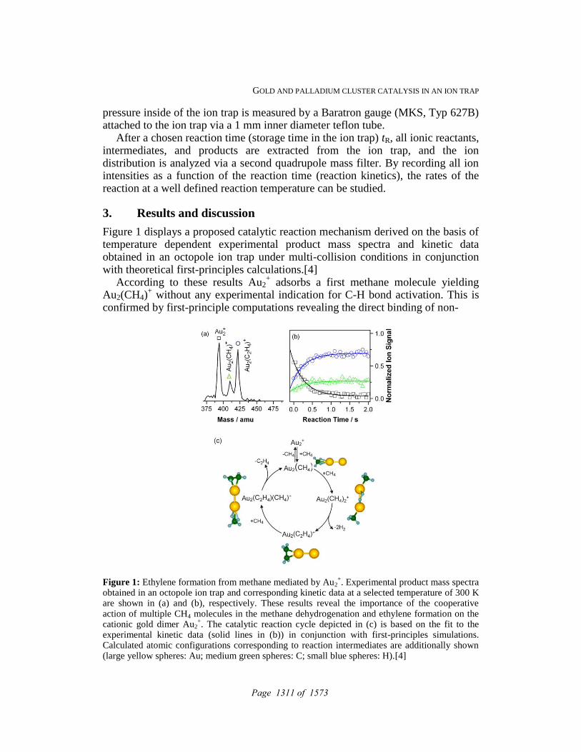
GOLD AND PALLADIUM CLUSTER CATALYSIS IN AN ION TRAP
pressure inside of the ion trap is measured by a Baratron gauge (MKS, Typ 627B) attached to the ion trap via a 1 mm inner diameter teflon tube.
After a chosen reaction time (storage time in the ion trap) tR, all ionic reactants, intermediates, and products are extracted from the ion trap, and the ion distribution is analyzed via a second quadrupole mass filter. By recording all ion intensities as a function of the reaction time (reaction kinetics), the rates of the reaction at a well defined reaction temperature can be studied.
3. Results and discussion
Figure 1 displays a proposed catalytic reaction mechanism derived on the basis of temperature dependent experimental product mass spectra and kinetic data obtained in an octopole ion trap under multi-collision conditions in conjunction with theoretical first-principles calculations.[4]
According to these results Au2+ adsorbs a first methane molecule yielding
Au2(CH4)+ without any experimental indication for C-H bond activation. This is
confirmed by first-principle computations revealing the direct binding of non-
Figure 1: Ethylene formation from methane mediated by Au2
+. Experimental product mass spectra
obtained in an octopole ion trap and corresponding kinetic data at a selected temperature of 300 K are shown in (a) and (b), respectively. These results reveal the importance of the cooperative action of multiple CH4 molecules in the methane dehydrogenation and ethylene formation on the cationic gold dimer Au2
+. The catalytic reaction cycle depicted in (c) is based on the fit to the
experimental kinetic data (solid lines in (b)) in conjunction with first-principles simulations. Calculated atomic configurations corresponding to reaction intermediates are additionally shown (large yellow spheres: Au; medium green spheres: C; small blue spheres: H).[4]
Page 1311 of 1573

GOLD AND PALLADIUM CLUSTER CATALYSIS IN AN ION TRAP
dissociated methane. However, the adsorption of a second CH4 molecule enables the activation and dehydrogenation of both methane molecules under formation of ethylene Au2(C2H4)
+ (see product mass spectrum in Figure 1a) and molecular
hydrogen. This C-H bond activation and subsequent dehydrogenation process was found to be only possible due to the cooperative action of two CH4 molecules. The direct desorption of the formed ethylene from Au2(C2H4)
+ was calculated to
be non-feasible, instead the coadsorption of a third CH4 is necessary yielding the experimentally observed intermediate Au2(C2H4)(CH4)
+. In this complex the
bonding of C2H4 to Au2+ is weakened and activated liberation of ethylene is
possible under thermal multi-collision conditions to close the catalytic reaction cycle by re-formation of Au2(CH4)
+.
A further example, which demonstrates the mutual O-O and C-H bond activation caused by cooperative coadsorption effects, is the reaction between the cationic gold dimer Au2
+ and a mixture of methane and molecular oxygen.[8] The
catalytic mechanism determined for this reaction is depicted in Figure 2. Similar to the above discussed reaction with CH4 only, the first reaction steps are described by the sequential adsorption of two methane molecules. Starting at a reaction temperature below about 270 K, the formation of Au2(CH4)2
+ then
enables the cooperative coadsorption of molecular oxygen yielding Au2(CH4)2O2+
although oxygen adsorption was found to be impossible in the presence of O2 only. Detailed molecular dynamics simulations revealed that the binding of O2 involves charge donation from the Au2(CH4)2
+ complex to the oxygen molecule
leading to O-O bond activation. This reaction mechanism is similar to the previously described mechanism for O-O bond activation on gold cations in the presence of molecular hydrogen.[3] The cooperative interaction of the activated O2 with CH4 finally leads to the activation of the strong C-H bond yielding the intermediate Au2(C3H8O2)
+ that is observed experimentally and shown
Figure 2: Proposed mechanism of the reaction of methane with molecular oxygen mediated by the cationic gold dimer Au2
+. The catalytic cycle was determined on basis of experimental kinetic data
obtained in an octopole ion trap in conjunction with first-principle calculations. Calculated atomic configurations corresponding to reaction intermediates are also depicted (yellow spheres: Au; green spheres: C; red spheres: O, blue spheres: H).[8]
Page 1312 of 1573

GOLD AND PALLADIUM CLUSTER CATALYSIS IN AN ION TRAP
theoretically to comprise formaldehyde and methane. The catalytic cycle is eventually closed by the elimination of two formaldehyde molecules under re-formation of Au2(CH4)
+.[8]
These selected examples emphasize the importance of the cooperative coadsorption concept for bond activation processes in nanocatalysis. This is further confirmed by our experiments with mass-selected palladium clusters in reaction with CD4. Palladium clusters form the smallest dehydrogenated products Pd2(C3D10)
+, Pd3(C4D10)
+, and Pd4(C4D14)
+ suggesting that on Pd2
+
the adsorption of a third CD4 immediately leads to the dehydrogenation, while on Pd3
+ and Pd4
+ four methane molecules are necessary for this reaction.[6] As
a consequence of the reversible reaction between Pd2+ with CD4 as well as of
Pd2(CD4)+ with CD4 it can be concluded that the cooperative action of three
CD4 molecules is mandatory for the dissociation of methane on Pd2+.
Particular advantages of gas phase clusters are their well-defined charge state and size and the possibility for a detailed theoretical investigation of these model systems. However, the latter examples also illustrate their potential to discover new chemical functionalities and here in particular to device strategies in the search for new reagents that enable selective C-H bond activation in small hydrocarbons and direct oxidation of methane with molecular oxygen which has not been achieved so far. Yet, this quest is at the heart of what has been called perhaps the most important scientific and technological challenge of the century:[11] The problem of developing energy resources with low environmental impacts.
References: [1] L.D. Socaciu, J. Hagen, T.M. Bernhardt, L. Wöste, U. Heiz, H. Häkkinen, U.
Landman, J. Am. Chem. Soc. 125 (2003) 10437. [2] S.M. Lang, D.M. Popolan, T.M. Bernhardt, in P. Woodruff (Ed.), Atomic
Clusters: From Gas Phase to Deposited, Elsevier, Amsterdam, 2007. [3] S.M. Lang, T.M. Bernhardt, R.N. Barnett, B. Yoon, U. Landman, J. Am. Chem.
Soc. 131 (2009) 8939. [4] S.M. Lang, T.M. Bernhardt, R.N. Barnett, U. Landman, Angew. Chem. Int. Ed.
49 (2010) 980. [5] S.M. Lang, T.M. Bernhardt, R.N. Barnett, U. Landman, Chem. Phys. Chem. 11
(2010) 1570. [6] S.M. Lang, T.M. Bernhardt, Faraday Disc. 152 (2011) 337. [7] S.M. Lang, T.M. Bernhardt, J. Chem. Phys. 131 (2009) 024310. [8] S.M. Lang, T.M. Bernhardt, R.N. Barnett, U. Landman, J. Phys. Chem. C 115
(2011) 6788. [9] T.M. Bernhardt, Int. J. Mass Spectrom. 243 (2005) 1. [10] R. Keller, F. Nöhmeier, P. Spädtke, M.H. Schönenberg, Vacuum 34 (1984) 31. [11] R.H. Crabtree, Chem. Rev. 110 (2010) 575.
Page 1313 of 1573

Proceedings of the 12th International Conference on Computational and Mathematical Methods in Science and Engineering, CMMSE2012 La Manga, Spain, July, 2-5, 2012
Prediction of Stable Low Density Materials Inspired by Nanocluster Building Block Assembly
Stefan T. Bromley1,2
1 Departament de Química Física and Institut de Química Teòrica i Computacional, Universitat de Barcelona, E-08028 Barcelona, Spain
2 Institució Catalana de Recerca i Estudis Avançats (ICREA), E-08010 Barcelona, Spain
email: [email protected]
Key words: Nanoclusters, Nanostructured Materials, Computaional Materials Science, Materials Design, Inorganic Materials
1. Introduction
The bottom-up approach to the design and understanding of new materials lies at the heart of the philosophy driving much of current nanotechnological research. One natural choice for nanoscale building units is well-defined nanoclusters that intrinsically display unusually high stability in vacuum. Cluster beams produced from bulk materials often yield the formation of certain clusters that are particularly favoured over others. Such “magic” clusters typically display relatively high symmetry and a large excess energetic stability over other cluster isomers of the same and similar composition. Numerous experiments have demonstrated the deposition of gas phase clusters, although due to the significant distribution of cluster size/type and the natural tendency of many cluster to coalesce the resulting deposited phase is typically amorphous. To exert some control over the structural stability of the synthesised material, “self-elected” magic clusters exhibiting strong and/or directional bonding would appear to particularly good candidates for nanoscale building blocks. Employing both global optimisation algorithms and ab initio quantum mechanical calculations, the computational approach to progress from nanoscale clusters to bulk materials is described with a number of concrete examples for a number of inorganic materials. Comparing with other known phases we find that many of our new nanocluster–based materials polymorphs are maginally
Page 1314 of 1573
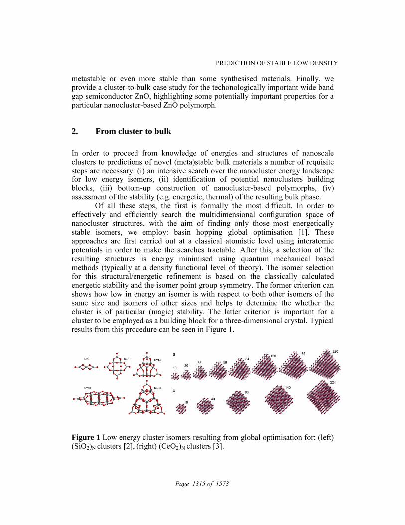
PREDICTION OF STABLE LOW DENSITY
metastable or even more stable than some synthesised materials. Finally, we provide a cluster-to-bulk case study for the techonologically important wide band gap semiconductor ZnO, highlighting some potentially important properties for a particular nanocluster-based ZnO polymorph.
2. From cluster to bulk
In order to proceed from knowledge of energies and structures of nanoscale clusters to predictions of novel (meta)stable bulk materials a number of requisite steps are necessary: (i) an intensive search over the nanocluster energy landscape for low energy isomers, (ii) identification of potential nanoclusters building blocks, (iii) bottom-up construction of nanocluster-based polymorphs, (iv) assessment of the stability (e.g. energetic, thermal) of the resulting bulk phase. Of all these steps, the first is formally the most difficult. In order to effectively and efficiently search the multidimensional configuration space of nanocluster structures, with the aim of finding only those most energetically stable isomers, we employ: basin hopping global optimisation [1]. These approaches are first carried out at a classical atomistic level using interatomic potentials in order to make the searches tractable. After this, a selection of the resulting structures is energy minimised using quantum mechanical based methods (typically at a density functional level of theory). The isomer selection for this structural/energetic refinement is based on the classically calculated energetic stability and the isomer point group symmetry. The former criterion can shows how low in energy an isomer is with respect to both other isomers of the same size and isomers of other sizes and helps to determine the whether the cluster is of particular (magic) stability. The latter criterion is important for a cluster to be employed as a building block for a three-dimensional crystal. Typical results from this procedure can be seen in Figure 1.
Figure 1 Low energy cluster isomers resulting from global optimisation for: (left) (SiO2)N clusters [2], (right) (CeO2)N clusters [3].
Page 1315 of 1573

PREDICTION OF STABLE LOW DENSITY
The transition from potential cluster building blocks to crystalline polymorph then follows by identifying crystal space groups compatible with the point group symmetry (i.e. the building block directional connectivity). Within these symmetry constraints one can then search for crystal structure types (e.g. via data mining hypothetical/experimental crystal structure databases) to use as topological templates to construct cluster-based materials. In Figure 2 we show two examples of this step.
Figure 1: Magic cluster based materials: (left) (SiO2)8 magic nanoclusters to nanoporous silica polymorph [4], (right): highly symmetric (ZnO)12 clusters to nanocage-based ZnO polymorph (SOD-ZnO) [5]. Once constructed, the cluster-based materials are evaluated with respect to their energetic, mechanical and thermal stability using periodic density functional calculations using the VASP code [6].
3. From cluster to bulk: ZnO case study
A possible alternative strategy to control optical/electronic properties of ZnO is not to induce modifications to the standard wurtzite crystal structure, but to attempt to change its polymorphic form. ZnO can exist in the zincblende structure, undergoes a transition to the rocksalt phase at ~9GPa and has been prepared as the h-BN structure in thin films. Recently we have predicted that the polymorphism is ZnO is likely to be much more wide-ranging [7], potentially allowing one to choose the properties of interest by changes in the crystal structure. Of all the new stable low density ZnO polymorphs, we predict one nanoporous structure, analogous to the silicate zeolite sodalite (SOD-ZnO) [3], to be particularly thermodynamically stable under appropriate conditions [8]. Via accurate electronic structure calculations we show that such low-density nanoporous ZnO polymorphs have surprising new properties suitable for extending the range of current ZnO applications. We specifically highlight the
Page 1316 of 1573

PREDICTION OF STABLE LOW DENSITY
prospective role of a cluster-inspired nanoporous ZnO polymorphs may have in hydrogen purification applications due to a novel multi-centre bond assisted transport mechanism [8] (see Figure 3).
Figure 3 Hydrogen atom transport through SOD-ZnO: (left) charge density of the H1s-Zn4s multicentre bond, (right) low barrier trajectory for H atoms to pass through the material. References:
[1] D. J. WALES AND J. P. K. DOYE, J. Phys. Chem. A 101 (1997) 5111. [2] S. T. BROMLEY, E. FLIKKEMA, Phys. Rev. Lett. 95 (2005) 185505. [3] A. MIGANI , K. M. NEYMAN, S. T. BROMLEY, Chem. Commun., 48
(2012) 4199. [4] J. C. WOJDEL, M. A. ZWIJNENBURG, S. T. BROMLEY, S. T. Chem.
Mater. 18 (2006) 1464. [5] J. CARRASCO, F. ILLAS, S. T. BROMLEY, Phys. Rev. Lett. 99 (2007)
235502. [6] G. KRESSE, J. HAFNER, Phys. Rev. B 47 (1993) 558.; G. KRESSE, J.
FURTHMÜLLER, Phys. Rev. B 54 (1996) 11169. [7] M. A. ZWIJNENBURG, F. ILLAS, S. T. BROMLEY, Phys. Rev. Lett.
104 (2010) 175503. [8] D. STRADI, F. ILLAS, S. T. BROMLEY, Phys. Rev. Lett. 105 (2010)
045901.
Page 1317 of 1573
Proceedings of the 12th International Conference on Computational and Mathematical Methods in Science and Engineering, CMMSE2012 La Manga, Spain, July, 2-5, 2012
Numerical Methods for the Intrinsic Analysis of Fluid Interfaces: Applications to Ionic Liquids
M. Natália D.S. Cordeiro 1 and Miguel Jorge
2
1 REQUIMTE, Faculdade de Ciências da Universidade do Porto, Rua
do Campo Alegre, 687, 4169-007 Porto, Portugal 2 LSRE/LCM – Laboratory of Separation and Reaction Engineering,
Faculdade de Engenharia da Universidade do Porto, Rua Dr. Roberto Frias, 4200-465 Porto, Portugal
emails: [email protected], [email protected]
Abstract
Key words: fluid interfaces, Molecular Dynamics simulations,
intrinsic analysis methods, ionic liquids surface
Starting by a general introduction on fluid interfaces, a quick review of the insights that have been obtained by applying molecular simulation methods to gather a detailed understanding of the structure and dynamic properties of such systems will be given. Special emphasis will be paid to the present available numerical methods that allow for an intrinsic analysis of fluid interfaces. We critically compare methods for identifying the true set of interfacial molecules and the calculation of density profiles, based on their reliability, robustness, and speed of computation. On the basis of this comparison, we propose a fast and accurate protocol to be routinely used for intrinsic surface analyses in computer simulations.[1,2] Then we give some numerical results to demonstrate the accuracy and efficiency of the proposed protocol forward probing the interfacial surface of room-temperature ionic liquids (IL). Specifically, we applied for the first time our proposed intrinsic analysis method, coupled with bivariate orientation analysis, to an IL surface (the room-temperature liquid/vapour interface of 1-nbutyl-3-methylimidazolium hexafluorophosphate, BMIM-PF6), demonstrating the broad spectrum of information one can obtain by
Page 1318 of 1573

INTRINSIC ANALYSIS OF FLUID INTERFACES
using these techniques. Our results suggest that experimental data should be reinterpreted considering a distribution of molecular orientations, rather than assuming a single preferred arrangement. The obtained results helped us resolving existing conflicts between simulations and experiments, and demonstrate the importance of intrinsic analysis techniques in the study of fluid interfaces.[3,4]
Molecule-fixed coordinate frame for the orientation studies of BMIM-PF6
Page 1319 of 1573

INTRINSIC ANALYSIS OF FLUID INTERFACES
The three most important molecular orientations of the BMIM cations
Acknowledgements This work is supported by projects PTDC/EQU-FTT/104195/2008, PEst-C/EQB/LA0020/2011 and Pest-C/EQB/LA0006/2011, financed by FEDER through COMPETE - Programa Operacional Factores de Competitividade and by FCT - Fundação para a Ciência e a Tecnologia..
References:
[1] M. JORGE, P. JEDLOVSZKY, M.N.D.S. CORDEIRO, A Critical assessment of methods for the intrinsic analysis of liquid interfaces. 1. Surface site distributions, J. Phys. Chem. C 114 (2010) 11169-11179.
[2] M. JORGE, G. HANTAL, P. JEDLOVSZKY, M.N.D.S. CORDEIRO, A critical assessment of methods for the intrinsic analysis of liquid interfaces. 2. Density profiles, J. Phys. Chem. C 114 (2010), 18656-18663.
[3] G. HANTAL, M.N.D.S. CORDEIRO, M. JORGE, What does an ionic liquid surface really look like? Unprecedented details from molecular simulations, Phys. Chem. Chem. Phys. 13 (2011) 21230-21232.
[4] G. HANTAL, I. VOROSHYLOVA, M.N.D.S. CORDEIRO, M. JORGE, A systematic molecular simulation study of ionic liquid surfaces using intrinsic analysis methods, Phys. Chem. Chem. Phys. 14 (2012), 5200-5213.
Page 1320 of 1573

Proceedings of the 12th International Conference on Computational and Mathematical Methods in Science and Engineering, CMMSE2012 La Manga, Spain, July, 2-5, 2012
Mathematical Model for Food Gums Using Non-Integer
Order Calculus
S. A. David1, A. H. Katayama
1 and C. Oliveira
2
1 Department of Basic Sciences, University of São Paulo - Brazil
2 Faculty of Energy Engineering, Fed. University of Dourados- Brazil
emails: [email protected] , [email protected], [email protected]
Abstract Fractional order calculus can represent systems with high-order dynamics
and complex nonlinear phenomena using few coefficients, since the arbitrary
order of the derivatives provides an additional degree of freedom to fit a
specific behavior. Numerous mathematicians have contributed to the history
of fractional calculus by attempting to solve a fundamental problem to the
best of their understanding. Each researcher sought a definition and therefore
different approaches, which has led to various definitions of differentiation
and antidifferentiation of non-integer orders that are provenly equivalent.
Although all these definitions may be equivalent, from one specific
standpoint, i.e., for a specific application, some definitions seem more
attractive. Furthermore, it is well known that food gums are complex
carbohydrates that can suit for a wide variety of functions in the context
of food engineering. The viscoelastic behavior of food gums is crucial for
these applications and formulations of new or improved food products.
Small progress has been made to understand the viscoelastic behavior of
food gums and there are few studies in the literature about these models. In
this paper, we applied the Riemann-Liouville approach and the Fourier
transform in order to obtain a fractional derivative model to make a
quantitative description of the viscoelastic properties behavior for a food
gum. The results reveal that the fractional model shows good simulation
capability and can be an attractive means for predicting and to elucidate the
dynamic viscoelastic behavior of food gums.
Key words: Fractional Calculus, Food Gums, Viscoelasticity
MSC2000: 47E99, 34B60
Page 1321 of 1573

Mathematical Model of Food Gums Using Fractional Order Calculus
1.Introduction
It is known that, historically, fractional calculus (FC) is the subarea of Science
that investigates and applies the concepts that involve derivatives of non-integer
order. However, until recently, applications involving derivatives and integrals of
non-integer order did not advance at the same pace as calculus of integer order.
Nevertheless, in the last few years, scientific and technological advances have
sparked renewed interest in this field of research. Many research centers,
particularly in Europe and the United States, have worked with FC applications
in, for example, physics, chemistry, wave diffusion and propagation, biology,
electromagnetism, image processing, and others.
With regard to its applications in food engineering, this area can be considered to
be practically untouched by this mathematical tool. That, allied to the fact that
food gums are complex carbohydrates with a variety of functions in the context of
food engineering, has motivated this project. Food gums are useful in the
production of many foods, e.g., in the design and modification of the texture of
the product. The viscoelastic behavior of food gums is crucial for applications that
involve new or improved formulations of food products.
In essence, the models thus developed can considered to comprise two parts: one
that involves the viscous behavior and another that involves the elastic behavior.
Few studies about these models are available in the literature, and therefore the
goal of this work is to use fractional calculus as a tool to model and simulate the
viscoelastic behavior of food gums.
2. Literature Review of Support
2.1 Food Gums
Gums present important properties for the food industry, such as thickeners of
aqueous solutions, dispersing agents, emulsion and suspension stabilizers,
stabilizers of room temperature, rheological and pseudoplastic properties, and
compatibilizers of food ingredients [16].
Gums are complex carbohydrates with various rheological properties that result in
viscoelastic behavior. According to Luvielmo et al. [16], xanthan gum solutions,
for example, are non-Newtonian fluids that are highly pseudo-plastic, i.e., their
viscosity decreases as the strain rate of the fluid increases. However, according to
Salah and Besbes [19], in 1978, Whitcomb and Macosko [20] investigated the
rheology of aqueous solutions of xanthan gum over a wide range of shear rates
and found that the solution behaves like a Newtonian fluid when sufficiently
diluted and at low shear rates. Studies conducted by Lopes da Silva et al. [15] and
Page 1322 of 1573

Mathematical Model of Food Gums Using Fractional Order Calculus
Kobayashi and Nakahama [13] presented positive results that increased the
understanding of the viscoelastic behavior of food gums. Understanding this
behavior by means of theoretical mechanisms can provide guidelines to relate the
behavior with the composition and structure. However, much remains to be
investigated through modeling and simulation of such gums in order to obtain
information to enable the right choice of this food ingredient. Moreover, such
investigations may lead to the discovery of solutions to further enhance the
attractiveness of food products that use such gums.
2.2 Fractional Calculus – Origins
The theory of fractional calculus dates back to the birth of the theory of
differential calculus, but its inherent complexity delayed the application of its
associated concepts. In fact, fractional calculus is a natural extension of classical
mathematics. Since the inception of the theory of differential and integral
calculus, mathematicians such as Euler and Liouville developed their ideas about
the calculation of non-integer order derivatives and integrals. Perhaps the subject
would be more aptly called “integration and differentiation of arbitrary order.”
The best-known definitions and gained more popularity in the scientific
definitions were the Riemann-Liouville and Grünwald-Letnikov [17]. Caputo[4]
reformulated the definition of fractional derivative given by the Riemann-
Liouville initial conditions so as to incorporate the integer order to solve
differential equations of fractional order. Many of the theories applied to the study
of (FC) has been developed in the second half of the nineteenth
century and, therefore, only in the twentieth century is that there have been
some applications of this theory in science and engineering areas.
Within this context, this topic can be considered "new", since there are about
thirty years held the first conference on the subject and the first
book entirely devoted to this subject was published in 1974 by K. B. Oldham and
J. Spanier [17]. Today, the list of texts and papers that refer to concepts and
applications of (FC) in several areas, for instance, control theory, diffusion
processes, electricity, modal analysis, among others, has already reached a high
number [1-3,6-10].
2.3 Fractional Calculus – Fundamentals
Numerous mathematicians have contributed to the history of fractional calculus
by attempting to solve a fundamental problem to the best of their understanding.
Each researcher sought a definition and therefore different approaches, which has
led to various definitions of differentiation and antidifferentiation of non-integer
orders that are provenly equivalent [17,18].
Page 1323 of 1573

Mathematical Model of Food Gums Using Fractional Order Calculus
Although Leibniz (1695), Euler (1730) andLaplace (1812) hadalready wondered a
bout the non-integer order derivatives, a first discussion about fractional
order calculus has been described by Lacroix in 1819,[18].Then, we
present this and other settings most recurrent and important:
i)Lacroix:
Lacroix expressed the nth derivative (for n ≤ m) in terms of Legrende’s symbol Г
for the generalized factorial. Recalling that
0
1 dteta ta (1)
and starting, for instance, with the function y = xm
, Lacroix expressed it as
follows:
nmnm
n
n
xnm
mx
nm
m
xd
yd
)1(
)1(
!)(
! (2)
ii) Liouville:
It was Liouville who engaged in the first major study of fractional calculus.
Liouville’s first definition of a derivative of arbitrary order ν involved an infinite
series. Here, the series must be convergent for some ν. Liouville’s second
definition succeeded in giving a fractional derivative of x -a
whenever both x and
are positive. Based on the definite integral related to Euler’s gamma integral, the
integral formula can be calculated for x –a
.
a
a
xa
a
xd
xd
)(
)(1 (3)
In order to verify this, one can note that:
0
1 dueu uxa (4)
if we change the variables t = x u , then
0
1
1
11
0
1 111dtet
xdt
xe
xx
tdt
xe
x
tdueu ta
a
t
a
at
a
uxa (5)
Thus,
0
1
0
1 1dtet
xdueu ta
a
uxa (6)
However, in accordance with equation (1), this yields the integral formula:
0
11dueu
ax uxaa
(7)
Page 1324 of 1573

Mathematical Model of Food Gums Using Fractional Order Calculus
Consequently, by assuming that axax eaedx
d
for any >0, then,
aa
a
xa
ax
a
a
xd
xd
)(
)(1
)(
)( (8)
The 1 term in the latter equation suggests the need to expand the theory to
include complex numbers.
Indeed, in terms of contemporary definitions, the modern theory of fractional
calculus is intimately connected with the theory of operators. In classical calculus,
the symbol n
xD is often used for the nth derivative operator (for n ≥ 0) while, less
commonly, 1
xD is used for the anti-derivative (or integral) operator.
A convenient notation described in [18] was the following: if υ is a positive real
number, )(xfDxc
denotes differentiation of order υ of the function f along the x-
axis. Similarly, the operator )(xfDxc
will denote integration of order υ of the
function f along the x-axis. Fractional calculus still lacks a geometric
interpretation of integration or differentiation of arbitrary order. Hence, the
subscripts c and x are called here terminals of integration instead of limits of
integration. This avoids unnecessary confusion.
iii) Riemann-Liouville:
Riemann-Liouville presented another definition of integration of arbitrary order >0 :
x
c
xc dttftxxfD11
)(
(9)
Let m where, for convenience, m is considered the smallest integer larger
than υ and 0 < ρ ≤ 1. Observe that,
)()( xfDxfD m
xcxc
(10)
Thus
)()( xfDdx
dxfD xcm
mm
xc
(11)
and consequently,
x
c
m
m
xcm
m
dttftxdx
dxfD
dx
d 11)(
(12)
or yet,
x
c
m
m
m
xc dttftxmdx
dxfD
11)(
(13)
Page 1325 of 1573

Mathematical Model of Food Gums Using Fractional Order Calculus
iv) Cauchy:
Cauchy’s definition, which is recognized as one that preserves some
important frequency properties [13], is expressed as follows:
d
tff
nt
)(
)()(
1
0
)(
(14)
v) Caputo:
In order to present Caputo’s fractional derivative, let m be the smallest integer that
exceeds α, thus enabling Caputo’s fractional derivative of order α > 0 to be
defined as follows:
t
m
m
dt
f
mtfD
0
1
)(
*)(
)(1)(
, m-1<α< m (15)
Although all these definitions may be equivalent, from one specific standpoint,
i.e., for a specific application, some definitions seem more attractive. In the
section 3, one can note the mathematical model involving the viscoelastic
behavior of food gums in the context of fractional order calculus.
3. Fractional Calculus - Modeling
It is a well-known fact that, for Newtonian viscous fluids, then following
relationship is applicable:
dt
dk
(16)
where is the shears stress, is the shear strain, is the shear strain rate , is
the viscosity and k is a constant. It is also well known that for elastic bodies
(Hookean):
0
0
dt
dkG
(17)
where is the shears stress , is the shear strain, G is the elastic modulus and k
is a constant. For a material that is neither a Hookean solid nor a Newtonian fluid,
one can think about following relationship:
dt
dk (18)
where k is a constant, 10 , is the shear stress and is the shear strain.
Based on the last equation that describes a linear viscoelastic behavior and by
applying the Boltzmann superposition principle using a fractional derivative
operator, the Eq. (18) has the following form:
n
n
dt
dk
N
n
n
1
(19)
Page 1326 of 1573

Mathematical Model of Food Gums Using Fractional Order Calculus
The Eq.(19) can be rewritten in terms of fractional derivative (Riemann-Liouville
approach), as follows:
)]([1
tDk n
N
n
n
(20)
The Eq. (20) will be investigated in order to describes a linear viscoelastic
behavior of a food gum in terms of fractional derivative. The theory of fractional
derivatives and Laplace transformers would be employed to manipulate these
material functions that need to be obtained.
With this fact in mind, one can write the fractional operator such as:
t
dtt
ttx
dt
dtxD
0
''
)'(
1
1)]([
(21)
with, .
The Leibniz rule may be used to differentiate the integral in Eq. (21) and
provides:
t
xttx
ttdt
dtxD
t
)1(
)0()'(
'
1
1
1)]([
0
(22)
By applying the Laplace transform to Eq. (22), the following expression is
obtained:
)]([ txD
[ ( ) ( )] ( )
(23)
Assuming that x(0) = 0 for all t<0 , Eq.(23) can then simplified to:
)]([ txD ( ) (24)
Now, by applying the Fourier transform to Eq.(24), a useful relationship is
produced as follows:
)]([ txD ( ) ( ) (25)
By applying Eq. (25) to Eq. (20), the following expression results:
)()()(1
nikN
n
n (26)
where )( and )(
means the complex stress and complex strain,
respectively, nk and na are constants and is the angular frequency.
The Eq. (26) is impractical because it involves a lot of constants. However, the
first two terms on the right side of Eq. (26) are chosen for approximation of
material function. Thus,
)(])()([)( 21
21 ikik (27)
where 1k , 2k , 1a and 2a are parameters of a simplified model.
In accordance to the theory of linear viscoelasticity, the complex modulus )(G ,
is defined as the ratio of complex stress to complex strain:
Page 1327 of 1573

Mathematical Model of Food Gums Using Fractional Order Calculus
)(
)()(
G (28)
By inserting Eq.(27) into Eq.(28) and after some algebraic manipulation, a
frequency-dependent complex modulus is obtained and by decomposing into real
and imaginary parts, the following expression is produced:
)(")(')( GiGG (29)
where,
)2
cos()2
cos()(' 221121 akakG
aa
(30)
)2
sin()2
sin()(" 221121 akakG
aa
(31)
The dynamic viscosity, ( ), and the out-of-phase component of the complex
viscosity, ( ), can be obtained by the following relationships:
)2
sin()2
sin()("
)( 2
1
21
1
1
' 21 akakG aa
(32)
)2
cos()2
cos()('
)(" 2
1
21
1
121 akak
G aa
(33)
The equations (30) ~ (33) can be used to simúlate a linear viscoelastic behavior of
a food gum since the constants in these equations be known.
With this fact in mind, we chosen a set of constants in order to investigate, by
means of numerical simulation, the viscoelastic behavior of the system. Some
results are presented in the next section.
4. Numerical simulation results
The table 1 shows the simulations cases with the model parameters.
1 10 100
0,01
0,1
1
10
100
Sto
rag
e a
nd
Lo
ss M
od
ulu
s, G
' an
d G
" [d
yn
/cm
²]
Storage Modulus
Loss Modulus
Frequency w [rad/s]
Fig.1: Case (a)
100
101
102
10
5
0
-5
Dynamic Viscosity n'
Out-of-phase Complex Viscosity
Dyn
am
ic V
isco
sity n
'
Frequency w [rad/s ]
Fig.2: Case (a)
Page 1328 of 1573

Mathematical Model of Food Gums Using Fractional Order Calculus
100
101
102
1
10
100
1000
Sto
rag
e a
nd
Lo
ss M
od
ulu
s, G
' an
d G
" [d
yn
/cm
²]
Storage Modulus
Loss Modulus
Frequency w [rad/s]
Fig.3: Case (b)
100
101
102
2,5k
2,0k
1,5k
1,0k
500,0
0,0
-500,0
-1,0k
-1,5k
Dynamic Viscosity n'
Out-of-phase Complex Viscosity
Dyn
am
ic V
isco
sity n
'
Frequency w [rad/s ]
Fig. 4: Case (b)
100
101
102
1
10
100
1000
Storage Modulus
Loss Modulus
Sto
rag
e a
nd
Lo
ss M
od
ulu
s, G
' an
d G
" [d
yn
/cm
²]
Frequency w [rad/s]
Fig 5: Case (c)
100
101
102
3k
2k
1k
0
-1k
-2k
Dynamic Viscosity n'
Out-of-phase Complex ViscosityD
yn
am
ic V
isco
sity n
'
Frequency w [rad/s ]
Fig. 6: Case (c)
10-2
10-1
100
101
102
10
100
1000
10000 Storage Modulus G'
Loss Modulus G"
Sto
rag
e a
nd
Lo
ss M
od
ulu
s, G
' an
d G
'' [d
yn
/cm
²]
Frequency w [rad/s ]
Fig. 7: Case (d)
100
101
102
4,0k
3,5k
3,0k
2,5k
2,0k
1,5k
1,0k
500,0
0,0
-500,0
-1,0k
-1,5k
-2,0k
Dynamic Viscosity n'
Out-of-phase Complex Viscosity
Dyn
am
ic V
isco
sity n
'
Frequency w [rad/s ]
Fig. 8: Case (d)
Page 1329 of 1573

Mathematical Model of Food Gums Using Fractional Order Calculus
Table 1 – Model parameters for the fractional calculus model
Case Concentration G’and G” a1 a2 k1 k2
(a) 0,5%
G’
G”
0,3444
0,1622
0,3430
0,1760
17,6
17,6
-15,8
-15,8
(b) 1,0%
G’
G”
0,1838
0,1313
0,1842
0,1318
37,0
-289,0
190
603
(c) 2,0%
G’
G”
0,2839
0,1380
0,2304
0,1382
-347
-94
655
484
(d) 4,0%
G’
G”
0,2296
0,1123
0,1646
0,1123
-407
-3992
1249
5035
5. Discussion and conclusions
In this article, we have investigated the concentrations dependencies of dynamic
viscoelastic behavior of a food gum using a fractional calculus model. The
fractional calculus was employed to make a quantitative description of the
viscoelastic behaviour. In conclusion, fractional calculus may be an alternative
and attractive means for predicting a linear viscoelastic behavior of food gums,
mainly, storage modulus (G’) and dynamic viscos ity (η’) versus frequency (ω),
for different concentration of food gum solution. We outline that the model
parameters for the numerical simulations were obtained from the experimental
data in the literature and a future research should be realized in order to verify real
physical meaning for the model parameters.
Acknowledgments:
This project was supported by São Paulo Research Foundation (FAPESP) through
grants no 2010/15824-0 and by a fellowship of the Dean’s Office for Research of
the University of São Paulo (USP).
References:
[1] Bagley, R. L., “Power law and fractional calculus model of viscoelasticity,
AIAA J. 27 ,1414-1417, (1989).
[2] Bohannan, G. W., “Analog fractional order controller in temperature and
motor control applications” , Journal of Vibrations and Control, Vol.14, pp. 1487-
1498, (2008).
Page 1330 of 1573

Mathematical Model of Food Gums Using Fractional Order Calculus
[3] Catania, G. et al. ,” A condensation technique for finite element dynamic
analysis using fractional derivative viscoelastic models “, Journal of vibration and
control, vol.14, pp. 1573-1586, (2008).
[4] Caputo, M. “Distributed order differentia equations modeling dieletric
induction and diffusion”, Fractional calculus and applied analysis, 4(4), 421-442
(2001).
[5] Caputo, M., Mainardi,F.,”Linear models of dissipation in anelastic solids”,
Rivista del NuovoCimento (SeriesII) 1, 161-198 (1971).
[6] David, S.A.,.“Investigation about fractional calculus in financial markets”. In
Proc: 7 th International Conference on Mathematical Methods in Science and
Engineering” – Chicago – IL -USA ( 20/06/2007 a 23/06/2007).pp. 148-154.
[7] David, S. A.; Linares, J. L.; Pallone, E. M. J. A. Fractional order calculus:
historical apologia, basic concepts and some applications.RevistaBrasileira de
Ensino de Física, v. 33, p. 4202, (2011).
[8] Dickinson, E. Hydrocolloids at interfaces and the influence on the properties
of dispersed systems.Food Hydrocolloids, 17,25–39, (2003).
[9] Espíndola,J.J., et al. “ Design of optimum systems of viscoelastic vibration
absorbers with a Frobenius norm objective function”, Journal of the Brazilian
Society of Mech. Eng. , vol. XXXI, no 3 , pp. 210-219, (2009).
[10] Espíndola,J.J., Bavastri,C. A., Lopes, E.M.O. , “ Design of optimum systems
of viscoelastic vibration absorbers for a given material based on the fractional
calculus model”, Journal of vibration and control, vol. 14, (2008).
[11] Herzallah, M. A. E., Baleanu, D., “Fractional-Order Variational Calculus
with Generalized Boundary Conditions”, Advances in Difference Equations,
Hindawi Publishing Corporation, doi:10.1155/2011/357580 , (2011).
[12] Kayacier, A.; Dogan, M. Rheological properties of some gums-salep mixed
solutions. Journal Of Food Engeneering, Kayseri, Turquia, p. 261-265. 08dez.
2004.
[13] Kobayashi, M.; Nakahama, N. Rheological properties of mixed gels.J.
Texture Studies 17, 161-174, (1986).
[14] Liu, S. H. “Fractal Model for the ac Response of a Rough Interface”,
Physical Review Letters.Vol.55 no. 5, pp. 529-532, July (1985).
[15] Lopes da Silva, J. A.; Gonçalves, M. P.; Rao, M. A. Viscoelastic behavior of
mixtures of locust bean gum and pectin dispersions.JournalofFoodEng., 18, 211-
228, (1993).
[16] Luvielmo, M. M.; Scamparini, A. R. P. Goma xantana: produção,
recuperação, propriedades e aplicação. Estudos tecnológicos – Vol. 5, nº1: 50-67,
(2009).
[17] Oldham,K.B.,Spanier, J., “The fractional calculus”, Academic Press, New
York, 1974.
[18] Ross Bertram , “Fractional Calculus”, Mathematics Magazine, vol. 50, no. 3,
pp. 115-122, Maio (1977).
Page 1331 of 1573

Mathematical Model of Food Gums Using Fractional Order Calculus
[19] Salah, R. B.; Besbes, S.; Chaari, K.; Rhouma, A.; Attia, H.; Deroanne, C.;
Blecker, C. Rheological and physical properties of date juice palm by-product
(Phoenix dactylifera L.) and commercial xanthan gums. Journal of Texture
Studies, p. 125-138. (2010).
[20] Whitcomb, P.J.; Macosko, C.W. Rheology of xanthan gum.J. Rheology 22,
493–505, (1978).
Page 1332 of 1573

Proceedings of the 12th International Conference on Computational and Mathematical Methods in Science and Engineering, CMMSE2012 La Manga, Spain, July, 2-5, 2012
Improving Metadata Management in a Distributed File System
Antonio F. Díaz, Mancia Anguita, Julio Ortega Department of Computer Architecture and Technology
University of Granada, Spain
emails: [email protected], [email protected], [email protected]
Abstract
Distributed file systems are good solutions in cluster storage for applications with extensive data computing. A challenge is how to efficiently organize data and metadata in order to provide a scalable solution with global high performance. In fact, metadata management is a key factor to achieve high access rates. We have developed a distributed file system (AbFS) to evaluate different algorithms to manage all file system operations. In this paper, we describe a new metadata management implemented in AbFS to improve scalability while maintaining good performance compared with other file systems. Key words: Distributed File Systems, metadata management
1. In tr oduction
Applications in high performance computing usually require file systems able to process big amount of data, so data servers could be severe bottlenecks. Also, it has been shown that metadata transactions account for more than 50 percent of all file system operations [1]. An optimized metadata management able to distribute requests among different servers can improve the overall performance. In recent years, different metadata management approaches have been developed to solve the partitioning problem of the namespace and inodes. Vesta, InterMezzo and Lustre [2] utilize hash-based mapping to achieve load balance and execute fast queries. Other solutions are dynamic tree partition and Bloom Filter-based [3] that can offer good performance. In this paper, we propose a hierarchical model to manage all the information related to data storage: meta-metadata information to distribute the metadata information among the storage space with a hybrid model and information about the data of the application.
Page 1333 of 1573

2. AbFS 0.2 Design
AbFS 0.2 is designed as a client-server system with a hierarchical model of 3 levels to control how and where to store all the file system data: meta-metadata, metadata and data. The meta-metadata daemon manages all resources, network interfaces, and volumes and determines how and where to store information. The global storage space is divided in chunks of data that can store metadata or data. AbFS stripes metadata and data across all volumes available (Fig. 1). The meta-metadata daemon runs in every server and synchronizes the changes in a quorum based model. Also, each server controls blocks used by files and stripped them across different volumes. In this way, the data from a file can be stored in different data servers.
Fig1. Meta-metadata distribution.
The metadata server is responsible to store metadata information from files and directories. Previous AbFS version 0.1, in [4] it is used a hash and subhash model which gave good results until about 4 million files in a file system. Hash techniques are fast with a moderate number of elements but its performance is low in large file system due to the sequential search inside each subhash. The new metadata approach here proposed combine hash and B+ trees. Hash distributes accesses among multiple medatata servers like previous version, using a partition based in name and parent inode numbers. Each metadata server store metadata in two B+ trees, that improve performance due to its O(log n) complexity. This new approach simplifies data distribution among servers and takes advantage of B+ tree speed. Moreover, servers include new metadata memory cache to improve performance. AbFS v0.2 stores name entries and inode in two different tables, that provide better hardware link support, inode delete operations and directory related operations. Previous version used a delegation table to distribute the name space with variable size depending of the number of servers. The new delegation table has a fixed size and stores the server with the information instead of the physical location. This approach reduces the migration performance penalty when the number of server
Page 1334 of 1573

grows. In AbFS v0.1, inodes had links with brothers and parents but, in the new version, directories just have to know if a directory has entries in another server. This is necessary to be sure that a directory is empty when it receives a remove operation. Metadata is stored in two tables to store lookup entries and inode information, respectively, as Figure 2 shows.
Fig.2 Hash/sub-hash metadata distribution in AbFS 0.1 and hash/B+/B+ approach in
AbFS 0.2.
Information stored in the lookup table is indexed by the tuple (Parent inode number, name), so it does not need extra information to index. Each entry stores the inode number related to the name. Also, this table is used to obtain the entries in a directory to process readdir operations. The second table stores inodes and is index by inode number. Changes in directories and files affect only to this table. Both tables have their own memory cache to speed up operations. In the new version, inode numbers and positions are now dynamic. The proposed model with metadata server in the user space performs very well. Metadata operations in the user space (e.g. create a file or a directory) are not penalized because each operation does not need a kernel call as other file systems need, in order to create another entry at lower level (ext3 or ext4). Most storage devices have slow response time so metadata operations in file system have to work asynchronously to achieve good performance. AbFS 0.2 implements servers in user space using complex cache mechanisms with parallel access.
3. Per formance Results
AbFS 0.1(server and client) was implemented in kernel space and AbFS 0.2 in user space (server) and in kernel space (client). To measure AbFS medatada performance, we have used mdtest in a cluster with two and four servers and up to 16 processes in 8 client nodes. Figure 3 shows files and directories creation performance (operations per seconds) for AbFS 0.1, 0.2 and Lustre with small number of files.
Page 1335 of 1573

Fig3. Metadata operations compared.
Fig3. Files and directories creation performance (operations per seconds) for AbFS 0.2, AbFS 0.1 and Lustre.
Fig. 4 shows the time for creating large number of files. AbFS 0.1 and 0.2 have similar latencies with small number of files, but AbFS 0.2 outperform AbFS 0.1 when a large number of files is created. Creation time increase with file numbers, but the B+ tree implementation of AbFS 0.2 improves the performance compared with the sub-hash AbFS 0.1 implementation for large number of files. Fig.4 Scalability of AbFS 0.2
4. Conclusions and Future Work
We have developed a new version of the distributed file system. AbFS 0.2 provides good performance compared with other file systems. Now, we are including new features to improve its scale behavior and its robustness.
5. Acknowledgments
The authors would like to thank FCSCL (Fundación Centro de Supercomputación de Castilla y León) for giving access to a cluster of its supercomputer Calendula. This work was partially funded by the project IPT-2011-1728-430000. References:
[1] D. Roselli, J.R. Lorch, and T.E. Anderson, “A Comparison of File System Workloads,” Proc. Ann. USENIX Technical Conf., 2000.
[2] P.J. Braam, “Lustre Whitepaper,” http://www.lustre.org, 2005. [3] Hua Y et al (2011) Supporting Scalable and Adaptive Metadata
Management in Ultralarge-Scale File Systems. IEEE Trans on Parallel and Distrib Syst 22(4):580-93
[4] Díaz, AF, Anguita M, Nieto E, Camacho HE and Ortega J, "A metadata management implementation for a symmetric distributed file system," in Proceedings of the 11th International Conference on Mathematical Methods in Science and Engineering, Alicante, 2011, pp. 1289-1297.
Page 1336 of 1573

Proceedings of the 12th International Conference on Computational and Mathematical Methods in Science and Engineering, CMMSE2012 La Manga, Spain, July, 2-5, 2012
COMPUTATIONAL SOFT MODELING OF VIDEO IMAGES OF A GAS-LIQUID TRANSFER
EXPERIMENT
Márcia M. C. Ferreira, Stephen P. Gurden, Cristiano G. de Faria
Institute of Chemistry, University of Campinas- UNICAMP, Campinas, SP, Brazil [email protected]
Abstract The use of chemical imaging is a developing area which has potential benefits for chemical systems where spatial distribution is important. In this work, the principal component analysis (PCA) and the regression method of partial least squares (PLS) were used to explore and to model the video images recorded during a laboratory experiment to investigate the distribution of carbon dioxide dissolved within a diffusion tank containing saline water. The experimental data was available as a movie stored on video tape. In order to perform the data analysis, it was necessary to transform the raw data into a form suitable for computational analysis. This involved digitization and reconciliation.
After reconciliation, a data array of size 300 600 3 52 was generated. Since the CO2 dissolution is related to the color of the solution, the main idea was to transform the multivariate color images, pixel by pixel, into univariate pH maps. In order to correct for intensity differences due to the uneven background illumination, pixelwise normalization was used prior to PLS modeling, in which each pixel was scaled to unit length: It was found that the pH map gives a more accurate representation of the differences in pH throughout the tank than is possible by a simple visual inspection of the original color image. The pH map is also more efficient than the principal component analysis (PCA) representation because it is a univariate representation of the one characteristic of specific interest: pH. The advantage of using this approach is that the Mapping reduces the wavelength mode of a multivariate image – from three to one in the case studied here – whilst retaining the full spatial detail.
Page 1337 of 1573

Proceedings of the 12th International Conference on Computational and Mathematical Methods in Science and Engineering, CMMSE2012 La Manga, Spain, July, 2-5, 2012
A Direct Algorithm for Finding Nash Equilibrium
Lun Shan Gao
THALES CANADA, 105 Moatfield Drive, Toronto, ON., CANADA
Email: [email protected]
Abstract
This study describes the relationship between the expected average payoffs of a two-person general-sum game and the fuzzy average of two linguistic values. A new algorithm for calculating Nash equilibria is introduced. The new algorithm transforms finding Nash equilibrium to solving linear equations
Key words: two-person general-sum game, mixed strategy, expected average payoff, linguistic variable, the fuzzy average, triangular fuzzy number, consequence matrix
1. Introduction
Paper [6] has discussed the application of the fuzzy average to two-person zero sum game theory. This study is an extension of paper [6].
For a given game in normal form, computing Nash equilibrium is a fundamental problem for algorithmic game theory. In two-person game theory, the expected average payoff is
defined as AqpTfor a player who has game matrix A . The expected average payoff is a
function of p and q , we denote it as ),( qpf . Finding Nash equilibrium is to find mixed
strategies p and q at where the function ),( qpf reaches its maximum value. If each
element in p and q is described with a probability density function (PDF for short), and
the PDFs are concave functions in R , finding the maximum values of function ),( qpf is
equivalent to solve the following equations.
0),( pqpf , 0),( qqpf .
However, it is usually complicated to solve the two equations, when p and q are a set of
PDFs respectively. It has been proven that finding Nash equilibria with traditional algorithms is intractable [11].
In this paper, instead of discussing the complexity of computing Nash equilibrium, we introduce a new algorithm to calculate Nash equilibria. The idea is to find the maximum
value of function ),( qpf . But instead of using PDFs, p and q are represented with a set
of triangular fuzzy numbers (TFNs for short), respectively. This paper includes the following sections. Section 2 gives brief reviews of the fuzzy average; Section 3 describes that an expected average payoff is identical to the fuzzy average; Section 4 gives the algorithm; Section 5 shows examples; Section 6 gives the conclusion.
Page 1338 of 1573

A DIRECT ALGORITHM FOR FINDING NASH EQUILIBRIUM
2. The Fuzzy Average
The fuzzy average [7] is defined as the average of values of a linguistic variable [17]. A linguistic variable is usually defined as (x, T(x), U, G, M), where x denotes the symbolic name; T(x) is a set of linguistic values that x can take; U is the physical domain that defines certain value; G is a syntactic rule which generates the values in T(x); and M is a mapping from the set T(x) to a set of fuzzy sets which are defined on U.
Let us consider the average of two values of a linguistic variable. Suppose that
),),(,( 1,11 MGUxTx and ),,),(,( 222 MGUyTy are two values of a linguistic variable
),,),(,( MGUxTx ,
where
,...,)( 211 mxxxxT , .,...,)( 212 nyyyyT
,...,,)(:)( 2111 mCCCxTxM , ,...,)(:)( 2122 nDDDyTyM .
),...1( miCi and ),...,1( njDj are TFNs which are defined on U. Without lose
generality, we suppose ]1,0[U . The fuzzy average is defined as follows.
ijm
i
n
j
DC ryxyxf ji 1 1
, )()()( (2.1)
where x U and y U; )(xiC and )(yjD are the membership functions of iC and
jD respectively; Rrij is the element of the consequence matrix.
For given x and y, )(xiC and )(yjD are required to satisfy (2.2) and (2.3).
),...1(0)( mixCi ,
m
i
Ci x1
)( = 1, (2.2)
),...1(0)( njyDj ,
n
j
Dj y1
)( = 1. (2.3)
Paper [6] has proved that (2.2) and (2.3) are satisfied when the mapping )(1 xM and
)(2 yM are fuzzy uniform mapping.
3. The Fuzzy Average and Expected Average Payoffs
Consider a bimatrix game (that is, two-person general-sum game with a finite number of
pure strategies) with nm payoff matrices )( ijaA and )( ijbB to player and ,
respectively. Let 1m probability vector p be a mixed strategy of player , 1n
probability vector q be a mixed strategy of player . Nash equilibrium for such a game is a point ),( 00 qp that satisfies the following relations:
00 Aqp T =
m
i
iiT
p
ppAqp1
0;1|max
00 Bqp T =
n
i
iiT
q
qqBqp1
0;1|max
Page 1339 of 1573

A DIRECT ALGORITHM FOR FINDING NASH EQUILIBRIUM
where
m
i
n
j
jijiT qapAqp
1 1
(3.1)
m
i
n
j
jijiT qbpBqp
1 1
(3.2)
are expected average payoffs of player and player , respectively.
Theorem 3.1.
For a two-person general-sum game, the fuzzy average (2.1) is identical to the expected average payoffs (3.1) or (3.2), if and only if the following is true.
(1) payoff matrix A or B is replaced with the consequence matrix )( ijr ,
(2) p and q are replaced with )(xiC and )(yjD , respectively,
(3) )(xiC and )(yjD satisfy (2.2)and (2.3), respectively.
Proof. According to the commutative and associative properties, (3.1) becomes
m
i
n
j
jiji qap1 1
=
m
i
n
j
ijji aqp1 1
)( (3.3)
for )(xiC and )(yjD satisfy (2.2)and (2.3), respectively, if we replace ip with )(xiC ,
jq with )(yjD and matrix A with consequence matrix )( ijr , then (3.3) is identical to the
fuzzy average (2.1). Therefore, (3.1) is equivalent to (2.1). Similarly, (3.2) is identical to (2.1).
For we distinguish the fuzzy averages of player and player in this paper, we use
)( , yxfA and )( , yxfB to represent the fuzzy average for player and player ,
respectively.
Theorem 3.2.
The fuzzy average )( , yxfA ( )( , yxfB ) has at least one maximum value in U, if function
)( , yxfA ( )( , yxfB ) is partial differentiable in U, and there exist UyUx 11 , which
satisfy (3.4) ((3.5)).
0),(
0),(
yyxf
xyxf
A
A
(3.4)
0),(
0),(
yyxf
xyxf
B
B
(3.5)
Proof: For ),( 11 yx is the solution of (3.4), )( 1,1 yxfA has an extremum value at ),( 11 yx .
On the other hand, since )(xiC is a concave function in U, for any UxUx 21 , and
]1,0[t , we have,
)()1()())1(( 2121 xtxtxttx CiCiCi
))1(( ,21 yxttxfA = ijn
i
m
j
DC ryxttx ji 1 1
21 )())1((
ijm
i
n
j
DCiCi ryxtxt j 1 1
21 )())()1()(( = ),()1(),( 21 yxftyxtf AA .
Page 1340 of 1573

A DIRECT ALGORITHM FOR FINDING NASH EQUILIBRIUM
Therefore, )( , yxfA is x concave. Similarly, one can prove that )( , yxfA is y concave as
well. That is, )( , yxfA is a concave function in U. Thus, )( , yxfA has a maximum value
at ),( 11 yx .
Theorem 3.3.
If ),( 00 yx is a solution of (3.4), and ),( 11 yx is a solution of (3.5), and
m
i
Ci x1
0 1)( ,
m
i
Ci x1
1 1)( ,
n
j
Dj y1
0 1)( and
n
j
Dj y1
1 1)( , then
))(),(( 00 yx DC and ))(),(( 11 yx DC are the mixed Nash equilibria of player and
player respectively, where
))()...(),(()( 002010 xxxx CmCCC , ))()...(),(()( 002010 yyyy DnDDD ;
))()...(),(()( 112111 xxxx CmCCC , ))(),...(),(()( 112111 yyyy DnDDD .
Proof. Since ),( 00 yx satisfies (3.4), according to Theorem 3.2, ),( 00 yxfA is a maximum
value of ),( yxfA . Similarly, ),( 11 yx satisfies (3.5), ),( 11 yxfB is a maximum value
of ),( yxfB . Based on the definition of Nash equilibrium, ))(),(( 00 yx BA and
))(),(( 11 yx BA are the Nash equilibria of player and player respectively.
4. The Algorithm
The algorithm in this paper is the extension of the fuzzy average applying to two-person zero-sum game [6]. As mentioned in previous section, each action which is taken by a player can be mapped into a possible range in the real number set. The possible range is represented with a TFN. That is, each action which is taken by a player is mapped into a TFN. The mean values of TFNs for player 1 divide the domain U into m-1 partitions; the mean values of TFNs for player 2 divide the domain U into n-1 partitions.
In order to calculate (3.4) and (3.5), the fuzzy average such as the average payoff function is required to be differentiable in U. However it is clear that the fuzzy average is not differentiable at the mean value of each TFN, but it can be differentiable within each partition which is divided by the mean values of TFNs.
The algorithm is as follows.
4.1. Define appropriate mappings )(1 xM and )(2 yM ;
4.2 Calculate (3.4) and (3.5) in each partition;
4.3. Solve linear equations for x and y respectively;
4.4. Find a maximum value in each partition;
4.5. Find the maximum value by comparing all the local maximum values.
Page 1341 of 1573

A DIRECT ALGORITHM FOR FINDING NASH EQUILIBRIUM
Readers may have the following questions. (1) Does Nash equilibrium depend on the
mapping? Namely, does the maximum value of )( , yxfA depend on the mapping? (2) Does
not )( , yxfA have a maximum value at a mean value of a TFN?
Nash equilibrium does not depend on the mapping because the solutions of (3.4) are
unique if )( , yxfA is differentiable in U. If )( , yxfA just has a maximum value at a divided
point, it is possible to miss the maximum value. However, that can be easily verified by
calculating )( , yxfA at the divided point.
5. Examples
Example 1. Consider a game with the following bimatrix.
)2,2
3()2
1,3()2,1(
)1,2()3,0()1,4(
By using traditional algorithm [5], the Nash equilibrium ),( ** qp is )74,73(* p and
)7
12
7
6,
7
1
7
5,(* xx
xq for ]2
1,0[x , the corresponding expected payoffs are,
74712*1 xv , 711*
2 v .
By solving (3.4) using the new algorithm, one can find the two Nash equilibria of
player as follows,
)0,,())(),(),((
),())(),((
21
21
413
412
411
32
31
322
321
DDD
CC
and
),,0())(),(),((
),())(),((
76
71
14133
14132
14131
74
73
742
741
DDD
CC
By solving (3.5), one can find the two Nash equilibrium of player as follows,
)0,,())(),(),((
),())(),((
72
75
713
712
711
74
73
742
741
DDD
CC
and
),,0())(),(),((
),())(),((
75
72
763
762
761
74
73
742
741
DDD
CC
The expected payoffs of player and player are as follows.
2),(4
13
2 Af ,7
1214
137
4 ),( Af ,7
117
17
4 ),( Bf ,7
117
67
4 ),( Bf , respectively.
Example 2. The Prisoner’s Dilemma. Consider the game with bimatrix
defectcooperate
defect
cooperate
)1,1()0,4(
)4,0()3,3(
Page 1342 of 1573

A DIRECT ALGORITHM FOR FINDING NASH EQUILIBRIUM
This bimatrix game does not have mixed strategy.
By using the new algorithm, one will realize that either (3.4) or (3.5) do not have a solution in this case. That tells us the following.
Proposition 5.1. For a finite bimatrix game, if (3.4) and (3.5) do not have a solution, then the bimatrix game does not have a mixed Nash equilibrium. It only has pure Nash equilibrium.
6. Conclusion
This paper has described a new algorithm for calculating Nash equilibria. Throughout the examples in section 5, it is clear that the new algorithm is efficient. It is simpler than Lemke-Howson algorithm.
When the distribution profile is represented with a set of TFNs, the new algorithm has exchanged the Nash equilibrium problem to solving linear equations in partition domains.
The application of the fuzzy average to two-person general-sum game can be extended to n-person non-cooperative game theory. This will be discussed in future study. By using computer, the new algorithm can solve large scale problems. This will be discussed in future study as well. Furthermore, one future study is to prove that the new algorithm is P-complete.
References:
[1]. AUBIN, J.P Mathematical Methods of Game and Economic Theory, North-Holland, Amsterdam, 1979
[2]. AUBIN, J.P ‘Fuzzy Core and Equilibrium of games Defined in Strategic form’, In: Ho, Y.C and Mitter, S.K: Directions in Large-Scale Systems, Plenum, New York, pp. 371-388, 1976
[3]. ARFI, B ‘Linguistic Fuzzy Logic Methods in Social Sciences’, STUDFUZZ 253, pp. 63-103.
[4]. DASKALAKIS, C, GOLDBERG, P and PAPADIMITRIOU, C 2006 ‘The Complexity of Computing a Nash Equilibrium’, STOC
[5]. FERGUSON, T.S, Mathematical Statistics- A Decision-Theoretic Approach, Academic Press, New York, 1967
[6]. GAO, L.S, ‘The discussion of Applications of the Fuzzy Average to Matrix Game Theory’, The proceeding of CCECE2012, 2012
[7]. GAO, L.S, ‘The Fuzzy Arithmetic Mean’, Fuzzy Sets and Systems, 107, pp. 335-348, 1999
[8]. GAO, L.S, ‘Studies on Application of Fuzzy Averaging in Numerical Analysis’, PhD thesis, Chiba University, Japan, 1995
[9]. GAO, L.S and KAWARADA, H, ‘Application of Fuzzy Average to Curve and Surface Fitting’, Proceeding of FUZZ-IEEE/IFES’1995
Page 1343 of 1573

A DIRECT ALGORITHM FOR FINDING NASH EQUILIBRIUM
[10]. KAUFMANN, A and GUPTA, M.M, Fuzzy Mathematical Models in Engineering and Management Science, Elsevier, Amsterdam, 1998
[11]. NISAN, N, ROUGHGARDEN, T, TARDOS, E and VAZIRANI, V.V, Algorithmic Game Theory, Cambridge University Press, 2007
[12]. NISHIZAKA, I and SAKAWA, M, ‘Equilibrium Solutions in Multi-objective Bimatrix Games with Fuzzy Payoffs and Fuzzy Goals’, Fuzzy Sets and Systems, 111:96-116, 2003
[13]. ORLOVSKI, S.A, ‘Fuzzy Goals and Sets of Choices in Two-Person Games’, Multiperson Decision Making Models using Fuzzy Sets and Possibility Theory, Kluwer Academic Publishers, Dordrecht, pp. 288-297, 1990
[14]. PELSCHUS, F and ZAVADSKAS, E.K, ‘Fuzzy Matrix Games Multi-Criteria Model for Decision-Making in Engineering’, INFORMATICA, Vol. 16, No. 1, pp107–120, 2005
[15]. WU, S.H and SOO, V.W, ‘Fuzzy Game Theoretic Approach to Multi-Agent Coordination’, T. Ishida: PRIMA’98, LNAI1599, pp. 76-87, 1999
[16]. ZHAO, J, , ‘The Equilibria of a Multiple Objective game’, Int. J. Game Theory, 20, pp. 171-182, 1991
[17]. ZIMMERMANN, H.J, Fuzzy Sets, Decision Making, and Expert Systems, Kluwer Academic, Boston, 1986
[18]. ZIMMERMANN, H.J, Fuzzy Set Theory and Its Application, 2nd
, Kluwer Academic Publishers, Boston, 1991
Page 1344 of 1573

Proceedings of the 12th International Conference on Computational and Mathematical Methods in Science and Engineering, CMMSE2012 La Manga, Spain, July, 2-5, 2012
Pole: A Planning Tool to Maximize the Network Lifetime in Wireless Sensor Networks
Antonio-Javier Garcia-Sanchez, Felipe Garcia-Sanchez, David Rodenas-Herraiz, Joan Garcia-Haro
Department of Information and Communication Technologies, Universidad Politécnica de Cartagena, (UPCT), Campus Muralla del
Mar, E-30202, Cartagena, Spain
emails: [email protected], [email protected], [email protected], [email protected]
Abstract
Network Lifetime is a crucial metric in the design of Wireless Sensor Networks (WSNs). They consist of hundreds or thousands of low-cost unmanned wireless nodes, the WSNs are mainly used to monitor outdoor scenarios (agriculture, forest, industry, etc.) over a large-period of time. However, nodes are energy constrained, which has a negative impact on both the node operation time and the network lifetime. To alleviate this effect, we propose a network planning tool, named Pole, intended to study the network lifetime metric extension, until the network operation made by the still alive wireless nodes is unfeasible. To this end, Pole combines a twofold procedure: (i) an optimization-based method to maximize network lifetime and (ii) an iterative process guaranteeing connectivity (that is satisfying at least a path between any arbitrary pair source-destination). Finally, Pole has been intensively evaluated and their outcomes are presented and discussed. Key words: Wireless Sensor Networks, Network Lifetime, Optimization, Network Planning Tool
Page 1345 of 1573

POLE: A PLANNING TOOL TO MAXIMIZE THE NETWORK LIFETIME IN WSNS
1. Introduction
Wireless Sensor Networks (WSNs) are formed by multiple unassisted embedded devices (nodes) which transmit data collected from different on-board physical sensors (temperature, humidity, pressure, etc.). The main advantage of WSNs is their ability to monitor large areas at low-cost, by deploying hundreds or thousands of resource-constrained nodes (memory, processing capability and energy- constrained), mainly, in outdoor scenarios (agriculture, forest, industry, etc.). In WSNs, energy limitations negatively impact on both the node operation time and the network lifetime. To alleviate this shortcoming, the appropriate cooperation among all network nodes is a crucial issue. The usual approach is that nodes work in a duty cycle (ON-OFF periods), where they perform their operations during the ON period of the cycle and then switch to the OFF (sleep) mode, therefore saving energy. Optimization techniques have usually been applied as useful network planning tools to learn the best cooperation among nodes. These techniques adjust the number of messages that must be dispatched by each node with the aim of decreasing its power consumption, and, as a consequence, extending the network lifetime. A longer network lifetime may pave the way to new WSNs-based services or to a better performance for existing WSNs applications. In this sense, several recent works may be found in the scientific literature [1-5]. Analyzing these works, we observed that the network lifetime is calculated as the time period during which the network operates until a node depletes its battery. However, the work in [6] defines a node -denoted as sink- that is able to establish, when a node fails, new communication paths to extend network lifetime. To this end, a complex algorithm is proposed for tree-based topologies, a particular mesh scenario, where a few nodes (called cluster-heads) are selected to transmit information to the sink. In [6], the authors point out that the network lifetime is only influenced by the energy consumption of the cluster-heads, because they handle all network traffic, thus consuming more energy than any other node (therefore cluster-heads become bottleneck nodes). In contrast, the idea behind our work is that any node is able to search different paths to the destination sink, alleviating the sink of this task and distributing the network traffic among all network nodes. Thus, our work applies to any mesh topology, where also each intermediate node fairly balances its traffic load (the total amount of messages handled by that node during a time unit period) among the nodes in its vicinity (neighbor nodes), maximizing the lifetime objective. In this paper we present and evaluate our planning tool for mesh networks (Pole) to maximize the network lifetime and to achieve a fair balancing of the traffic load. Network lifetime is computed by means of an iterative procedure, where each iteration is an independent stage that starts with a network planning to maximize network lifetime and finalizes when a node fails per depletion of its
Page 1346 of 1573

POLE: A PLANNING TOOL TO MAXIMIZE THE NETWORK LIFETIME IN WSNS
battery (dead node). The last iteration is reached when the number of dead nodes is such that an active node becomes isolated, that is, there is not any path through any neighbor node that communicates this isolated node with the sink. Finally, the total lifetime is calculated as the sum of the network lifetimes obtained by each iteration. The rest of the paper is organized as follows. Section 2 formulates and solves the optimization problem by using linear programming, presenting in turn the planning tool proposed. Section 3 shows and comparatively discusses the performance evaluation results obtained from our analysis. Finally, Section 4 concludes.
2. Problem Formulation: The Pole planning tool
As it can be noted from the previous discussion, network lifetime is a key issue that fully affects the development of new WSNs applications and/or the operation/performance of already existing deployments. Thus, prolonging the network lifetime implies an important contribution in WSNs field. In this context, we propose a procedure based on maximizing the network lifetime metric by appropriately involving all network nodes. When a node depletes its battery, our solution re-designs the network so that a dead node does not affect data transmission of the remaining nodes with the destination (sink) node. Thereby, the network will still continue their operation, thus extending its lifetime. Our contribution consists of designing a planning tool for arbitrary mesh networks called Pole. To facilitate its understanding, we have divided the operation of Pole into the following stages: 1. Maximizing the network lifetime from the initial amount of node’s energy
(initial node power level). Pole generates all the possible paths from any network node to the destination sink through the intermediate/routing nodes closer to the sink. In addition, Pole guarantees a balanced traffic load per link. This means that the messages dispatched by a node are fairly distributed by each connecting link with its neighbors.
2. When a node fails (dead node by depletion of its battery), Pole finishes the current iteration and calculates the network lifetime. If all remaining network nodes have at least a path to transmit their data to the sink, Pole starts a new iteration. The objective is again to plan the network, balancing the new traffic loads per link and maximizing the network lifetime objective but now discarding dead nodes and taking into account the current residual battery level of still active nodes.
3. Finally, the algorithm ends its operation when a node is isolated, that is,
this node is not able to establish any link with the nodes in its vicinity.
Page 1347 of 1573

POLE: A PLANNING TOOL TO MAXIMIZE THE NETWORK LIFETIME IN WSNS
To this end, a linear programming (LP) optimization is applied from iteration 1 (and, if appropriate, subsequent iterations) having into account the following assumptions: (i) Random mesh topologies are selected, (ii) the information flows from any node to a unique sink or base station (in our case, a special node denoted by number 1 without energy limitations) and (iii) any node may transmit data to their neighbors in coverage closer to the sink. Under these assumptions, the LP formulation for our model is as follows:
Maximize TNETWORK (2) Subject to: ijth >0, TNETWORK >0, jiNji ,),( (3)
ji
N
jijij Rth
1
+ ij
N
jjiji Rth
1
jiiNi ,1,
(4)
ji
N
jijijtx RthE
1
+ ij
N
jjijirx RthE
1
+ sidualEReNETWORK
source
T
E ;
0,,1, sourceEjiiNi (5)
ijth (6)
Where:
Parameter Description N Number of nodes of the WSN
ijth Achieved throughput of the link ij. Throughput is a metric which defines the bits per second (b/s) transmitted by node i to its neighbour node j (see Figure 1)
ij Parameter indicating the existence of a link between nodes i and j. If ij =1, there is a link; otherwise ij =0
jiR When a message is transmitted to a node, this parameter indicates if this node is nearer to the sink than transmitter one. If jiR =1, the
node selected is nearer to the sink; otherwise jiR =0
Node transmission bit rate (bits per second, b/s) Maximum WSN transmission bitrate (bits per second, b/s) TNETWORK Network lifetime
Page 1348 of 1573

POLE: A PLANNING TOOL TO MAXIMIZE THE NETWORK LIFETIME IN WSNS
txE Energy consumed by the transmission of a message in joules per bit
rxE Energy consumption to receive a message in joules per bit
sidualERe Energy consumed in the time periods where there is no messages transmission/reception. It is expressed in joules per second.
sourceE Initial energy for the node i in joules
Table 1. Description of each parameter for the LP model under study
Table 1 shows the parameters employed in the LP problem formulation. Expressions (1) to (5) are the objective functions and inequality/equality constraints for the network lifetime maximization problem:
Expression (2) avoids any throughput and lifetime lower than zero. They are not valid values.
Expression (3) represents the throughput conservation for each node, i.e. the summation of the outgoing throughput plus the incoming throughput of a node i must be less than or equal to the maximum transmission data rate offered by the node.
Expression (4) models the energy constraints of a node. Expression (5) limits the achieved throughput per link to the maximum
transmission rate (250 kbps) specified by the IEEE 802.15.4 [7], standard de facto of WSNs.
Node i
Node1
Node2
Node j
Nodek
Linki1
Linki2
Linkij
Linkik
Figure 1. Links and achieved throughputs for node i and its neighbors
Page 1349 of 1573

POLE: A PLANNING TOOL TO MAXIMIZE THE NETWORK LIFETIME IN WSNS
On the other hand, expressions (1)-(5) obtain the value of the balanced throughput per link ( ijth ). These values are introduced into the next equation (6) to calculate
the balancing traffic load per link:
Traffic Loadij = 100
1
kz
ziz
ij
th
th ijth > izth >0 jiNji ,),( (6)
Where
mz
zizth
1
is the total throughput generated by node i. It is calculated as the
sum of the achieved throughputs of all links that connect i with its neighbors (see Figure 1). The optimization process finalizes when one or more nodes reach their energy-constrained capabilities. Under these conditions, the planning tool runs the iterative algorithm 1 below (pseudocode): Algorithm 1 (1) Do for each node i jiiNi ,1,
(1.1) If there is not any node j that satisfies ( 1 ij and jiR =1 ), this
means that there is not an available path between node i and the sink. (1.2) else there is an available path. (2) Do while the TLifetime changes, (2.1) if all active network nodes have a path to the sink. (2.1.1) Update TLifetime as TLifetime + TNETWORK
(2.1.2) In the first iteration update:
Enode = Esource-[ ji
N
jijijtx RthE
1
+ ij
N
jjijirx RthE
1
+ sidualERe ] TNETWORK
In the remaining iterations update:
Enode= Enode -[ ji
N
jijijtx RthE
1
+ ij
N
jjijirx RthE
1
+ sidualERe ] TNETWORK.
(2.1.3) Run steps (1)-(5) of the LP optimization but substituting in the equation (4) the parameter Esource by Enode.
Page 1350 of 1573

POLE: A PLANNING TOOL TO MAXIMIZE THE NETWORK LIFETIME IN WSNS
(2.2) else there is an available path, the current value TLifetime is the total value of the network lifetime. End algorithm In algorithm 1, step 1 discovers the existence of isolated nodes. These nodes lack links with its vicinity into its coverage range. In contrast, if all active networks nodes have a path to the sink, step 2.1 runs the LP problem again, obtaining the traffic load per link and optimizing the network lifetime. In each iteration, before executing the LP part, the current value of the node’s energy (Enode) is introduced into equation (4) (the residual battery level of the node). Finally, if a node becomes isolated, step 2.2 presents the total network lifetime (TLifetime) as the sum of TNETWORK of all the Pole iterations.
3. Numerical Results
To conduct the evaluation, different WSN random topologies formed by a fixed number of nodes (ranging from 16 to 99 nodes) were selected. Links are established when the distance between neighbor nodes is less than or equal to 100 meters (usual coverage distance of wireless nodes on direct vision). Furthermore, the network coordinator is the sink/base station node appointed to receive all network data. As any other network node, the coordinator was randomly placed at the network and labeled as node 1. The remaining network nodes deliver information to the coordinator. Additionally, we have considered that all nodes dispatch sensing data at constant rates of 1 message per second. Finally, Table 2 shows the values of parameters employed in our evaluation.
Parameter Value N Networks formed by 16, 49 and 99 nodes 256 bits per second 250 kbits per second
txE 6103048.0 joules per bit
rxE 6103324.0 joules per bit
sidualERe 61060 joules per second.
sourceE 64800 joules
Table 2. Value of each parameter employed in our numerical evaluation Figures 2 and 3 depict two topologies formed by 16 and 99 nodes, respectively. In both scenarios, the first nodes that deplete their batteries are neighbors of the sink. They concentrate the greater amount of messages of the network, and, as a consequence, they consume more energy than the remaining nodes in the processes of transmission and reception of messages. Both figures also verify the operation of the Pole planning, extending the network lifetime until one
Page 1351 of 1573

POLE: A PLANNING TOOL TO MAXIMIZE THE NETWORK LIFETIME IN WSNS
intermediate node is not able to connect with any neighbor node. For instance, Figure 2 shows how node 11 is the first node failing that is depleting its battery. When it occurs, nodes transmitting to node 11 must switch their transmissions to other neighbor nodes in coverage. In particular, neighbor nodes 6, 8 and 10 switch to nodes 4 and 9 to continue with their data transmissions to the sink. The process follows until node 12 is dead. Then, a significant amount of network nodes are isolated. As a consequence, there is not a path between these nodes and the sink, the dispatching of their sensing data being unfeasible. Under the same circumstances and to the best of our knowledge, most of the works that deal with the same topic would finalize its process when node 11 has fallen. In comparison with these works, our design implies extending the network lifetime about 27% in the case of the 16 nodes topology, and 71% in the case of 99 nodes.
0%20507090100%
0%20507090100%
0%20507090100%
0%20507090100%
(1) (2)
(3) (4)
0%20507090100%
0%20507090100%
0%20507090100%
0%20507090100%
0%20507090100%
0%20507090100%
0%20507090100%
0%20507090100%
(1) (2)
(3) (4)
Figure 2.Topology of 16 nodes. Subfigures (1)-(4) show the sequence of the traffic load balancing and the increasing of the Network lifetime metric
Page 1352 of 1573

POLE: A PLANNING TOOL TO MAXIMIZE THE NETWORK LIFETIME IN WSNS
0%20507090100%
0%20507090100%
(1) (2)
0%20507090100%
0%20507090100%
0%20507090100%
0%20507090100%
(1) (2)
Figure 3. Network lifetime and % traffic load results obtained for a topology of 99 nodes
Figure 4 shows a network made by 49 nodes. The singularity of this topology is in the location of the nodes. On the one hand, a high node density monitors a given area, which is placed remotely from the sink. On the other hand, the information generated by this zone is dispatched to the sink thanks to a few intermediate nodes. Thus, they centralize the transmission of sensing data, resulting in greater energy consumption than the remaining nodes, and becoming the network bottleneck. Finally, Figure 5 shows a high density of nodes in the proximity of the sink. In this case, Pole assures a balancing of messages on the entire network. To this end, each node fairly distributes its traffic load through the links with its neighbors, what leads to maximize the network lifetime. Considering this scenario, there is not a pattern for the death of the nodes, that is, any network node can be the following in depleting its battery.
0%20507090100%
0%20507090100%
(1) (2)
0%20507090100%
0%20507090100%
0%20507090100%
0%20507090100%
(1) (2)
Figure 4. Network lifetime and percentage of traffic load outcomes obtained by a topology of 49 nodes. Subfigure (1) shows results when node 13 depletes its battery. Subfigure (2) shows results
when node 4 fails (its battery depletes) and, as a consequence, the operation of the network finalizes
Page 1353 of 1573

POLE: A PLANNING TOOL TO MAXIMIZE THE NETWORK LIFETIME IN WSNS
(1)
(2)
(3)
(4) (8
)(5
)(6
)(7
)
(12)
(11
)(1
0)
(9)
(13)
(14
)
Figure 5. Scenario with a high node density. Sequence of subfigures (1)-(14) depicts the increase
of Network lifetime and the balancing of traffic load
Page 1354 of 1573

POLE: A PLANNING TOOL TO MAXIMIZE THE NETWORK LIFETIME IN WSNS
4. Conclusions and Future Research
In this paper, we propose a network planning tool whose main contribution is to extend the network lifetime of a WSN deployment. This tool, named Pole, is based on an iterative maximization process for the metric network lifetime. In comparison with other similar algorithms designed for optimizing the lifetime until the first node dies, Pole takes advantage of extending the network lifetime while all the nodes still alive have a path to the sink. Additionally, our tool achieves a fair balancing of the traffic load per link, what leads to coordinate the entire network nodes with the goal of saving their power consumptions. Our future research in this field is aimed at further improving our mathematical optimization model, including new objectives and constraints. For instance, the optimization of the node positions within the deployment area could provide a larger energy saving. On the other hand, the inclusion of new constraints aimed at estimating the ratio of dead nodes on the sensed area will help in gaining insight into the feasibility of the network. Acknowledgements This research has been supported by the MICINN/FEDER project grant TEC2010-21405-C02-02/TCM (CALM). It is also developed in the framework of “Programa de Ayudas a Grupos de Excelencia de la Región de Murcia, de la Fundación Séneca, Agencia de Ciencia y Tecnología de la RM”. References:
[1] Y. T. HOU, Y. SHI, and H. D. SHERALI, Rate Allocation and Network Lifetime Problems for Wireless Sensor Networks, IEEE/ACM Transactions on Networking, vol. 16, no. 2, pp. 321-334, Apr. 2008.
[2] L. SHU, M. HAUSWIRTH, Y. ZHANG, J. MA, G. MIN and Y. WANG, Cross Layer Optimization for Data Gathering in Wireless Multimedia Sensor Networks within Expected Network Lifetime, Journal of Universal Computer Science, 16 (2010) 1343-1367.
[3] V. MHATRE and C. ROSENBERG, Energy and cost optimizations in wireless sensor networks: A survey, Performance evaluation and planning methods for the next generation Internet. Springer, 2005, pp. 227-248.
[4] A. MUNIR and A. GORDON-ROSS, Optimization Approaches in Wireless Sensor Networks, Sustainable Wireless Sensor Networks (2010) 313-338.
[5] M. X. CHENG, X. GONG, L. CAI, and X. JIA, Cross-Layer Throughput Optimization With Power Control in Sensor Networks, IEEE Transactions on Vehicular Technology, 60 (2011) 3300-3308.
[6] F. V. C. MARTINS, E. G. CARRANO, E. F. WANNER, R. H. C. TAKAHASHI, and G. R. MATEUS, A Hybrid Multiobjective Evolutionary Approach for
Page 1355 of 1573

POLE: A PLANNING TOOL TO MAXIMIZE THE NETWORK LIFETIME IN WSNS
Improving the Performance of Wireless Sensor Networks, IEEE Sensors Journal, 11 (2011) 545-554.
[7] IEEE Standard for Information Technology-Telecommunications and Information Exchange Between Systems-Local and Metropolitan Area Networks- Specific Requirements Part 15.4: Wireless Medium Access Control (MAC) and Physical Layer (PHY) Specifications for Low-Rate Wireless Personal Area Networks (WPANs), IEEE Std 802.15.4-2006 (Revision of IEEE Std 802.15.4-2003), pp. 1-305, 2006.
Page 1356 of 1573

Proceedings of the 12th International Conferenceon Computational and Mathematical Methodsin Science and Engineering, CMMSE2012La Manga, Spain, July, 2-5, 2012
Gallium Clusters: from superheating to superatoms
N. Gaston1*, D. Schebarchov1, and K. G. Steenbergen2
1 MacDiarmid Institute for Advanced Materials and Nanotechnology, Industrial Research Ltd, New Zealand
2 School of Chemical and Physical Sciences, Victoria University of Wellington, New Zealand
*Corresponding author: Email [email protected]
Abstract
We present the results of first-principles studies of the electronic structure of gallium clusters, the relationship between the electronic structure and the geometric structures of the clusters, and relate this to the polymorphism of the bulk metal.
Key words: gallium, metal clusters, superheating, superatoms
1. Introduction
Gallium is a highly polymorphic element with a rich phase diagram, a challenge to theory. A considerable body of work shedding light on how the different phases of gallium come about has been generated by synthetic chemists, who have successfully isolated and characterised a range of metastable gallium cluster compounds [1]. We rationalise these metastable clusters through a detailed assessment of the underlying electronic structure [2].We have investigated two distinct classes of cluster; close-packed, as would be typical for a bulk metal, and a second class with a hollow icosahedral centre. Somewhat surprisingly, our analysis of the electronic structure provides evidence for a clear relationship between these icosahedral motifs and the ground-state phase of bulk gallium metal. The set of gallium clusters considered here exhibits a clear trend, demonstrating how local structure, ligand- and crystal-field effects can systematically alter the superatom electron shell structure in clusters.
Page 1357 of 1573

GALLIUM CLUSTERS: FROM SUPERHEATING TO SUPERATOMS
2. Superheating gallium clusters
The experimental discovery of superheating in gallium clusters [3] contradicted the clear and well-demonstrated paradigm that the melting temperature of a particle should decrease with its size [4]. The observed extremely sensitive dependence of melting temperature on size goes to the heart of cluster science, and the interplay between the effects of electronic and geometric structure [5]. In the case of gallium, the extreme polymorphism displayed by the bulk metal introduces additional complications. We have used our understanding of the dimeric bulk structure of gallium to elucidate the patterns of bonding in the clusters, which also display dimeric structural motifs for small sizes. In particular, we consider the implications of the generally linear relationship of melting temperature and cohesive energy for elemental solids, which is that the low melting temperature of gallium corresponds to the melting of a molecular solid. We explore the nature of both inter- and intra-molecular bonding of the Ga2 dimer and relate this to structures of the small clusters, and their melting behaviour. We present results of a parallel tempering molecular dynamics study of the melting behaviour of small gallium clusters, and compare the influence of small-core vs large-core pseudopotential, charge, and structural isomer on the description of melting. We consider the relationship between electronic and geometric structure in these small clusters, and relate this to the well-known polymorphism displayed by elemental gallium in the bulk.
Fig. 1. The electronic structure of metalloid gallium clusters corresponds to jellium-like closed electronic shells.
Page 1358 of 1573

GALLIUM CLUSTERS: FROM SUPERHEATING TO SUPERATOMS
Fig. 2: We observe distinct melting behaviours of neutral and cationic clusters.
As shown in Fig. 2, the specific heat curves obtained for cationic clusters are clearly distinct from those obtained for the neutral clusters. By exploring the melting behaviours of different structural isomers, we are able to determine to what effect these differences are due to isomeric structure, and the effect of charge.
Acknowledgements
This work has been supported by the Marsden Fund of the Royal Society of New Zealand under contract IRL0801. We also thank the BlueFern supercomputer team at the University of Canterbury for technical support and computer time. Use of the Center for Nanoscale Materials was supported by the U. S. Department of Energy, Office of Science, Office of Basic Energy Sciences, under Contract No. DE-AC02-06CH11357.
References:
[1] Schnepf and Schnöckel. Angew. Chem. Int. Ed. 41, 3532-3554 (2002) [2] D. Schebarchov and N. Gaston, Phys. Chem. Chem. Phys. 13, 21109-
21115 (2011)
Page 1359 of 1573

GALLIUM CLUSTERS: FROM SUPERHEATING TO SUPERATOMS
[3] G. A. Breaux, R. C. Benirschke, T. Sugai, B. S. Kinnear, and M. F. Jarrold, Phys. Rev. Lett. 91, 215508 (2003)
[4] P. Pawlow, Z. Phys. Chem. 65, 1 (1909)[5] M. Schmidt, R. Kusche, B. von Issendorff, and H. Haberland, Nature 393,
238 (1998)
Page 1360 of 1573

Proceedings of the 12th International Conference on Computational and Mathematical Methods in Science and Engineering, CMMSE2012 La Manga, Spain, July, 2-5, 2012
Born Oppenheimer DFT molecular dynamics and DFT-MD methods for biomolecules
A. Goursot1, T. Mineva1 and D.R. Salahub2
1 ICGM, UMR5253, Ecole de Chimie de Montpellier, France 2 Departmentof Chemistry, University of Calgary, Canada
Emails:[email protected], [email protected],
Abstract
BOMD-MD (QM/MM) methodologies have been applied to glycine in water. These developments have been implemented in the deMon2k program. The intramolecular proton transfer has been observed during the dynamics at 300K and the calculated free energy changes of the reaction path are in good agreement with experimental values and competitive with AIMD results. Key words: DFT, BOMD-MD, QM/MM-MFEP MSC2000: AMS Codes (optional)
1. Introduction
Atomistic simulations of biomolecules remain one of the challenges of present day computational chemistry and biophysics. In such simulations one of the main difficulties is to both give an accurate description of the structural and energetical aspect of the biochemical processes, while simulating very large systems for the lengths of time relevant to the studied problems. If one is particularly concerned by properties strongly related with electronic structure accuracy, such as bond breaking/making, transition metal sites, magnetic properties and sufficiently accurate energetic (for example relative energies of different conformers), the choice of methods is restricted to methods based on the calculation of the full electronic structure of the system. These electronic structure, or quantum mechanical (QM) methods, are usually based on the Density Functional Theory (DFT). Despite the large development of computer and code performances, the size of the biosystem remains unfortunately limited to about 1000 atoms for geometry optimization and 150 atoms for reasonably long dynamics. Moreover, taking into account the solvent, when a global treatment is not sufficient, is still increasing the computational demand. Hybrid methods where the system is partitioned into a
Page 1361 of 1573

BOMD-MD FOR BIOMOLECULES
chemically active part, treated by first-principles QM methods and a larger environment, assumed to be chemically inert, which is modeled by a classical molecular mechanics (MM), have been introduced in the late 70s and have incorporated technological improvements along the years. They have been shown successful for studying chemical reactions in solution, catalytic and biological systems, including enzymatic reactions [1-3]. This hybrid QM/MM methodology looks particularly attractive for reproducing solvent effects when a discrete representation of the solvent molecules is needed, which is the case in most biosystems and processes of our interest. In fact, comparison of full QM and QM/MM results for sufficiently small peptides in water have been recently performed, including eventually an analysis of full MM results [4,5]. These comparative studies led to the following main conclusions: (i) the solvation pattern around most groups of the dipeptides are similarly described by the three methods; (ii) solvation patterns around terminal -CO2- and -NH3
+ groups are poorly reproduced in MM simulations; (iii) solvation patterns of the full QM results are well reproduced, at a lower cost, by the QM/MM calculation involving MM waters; (iv) DFT/MD computed chiroptical properties of a solvated glycine molecule are comparable to those obtained with the much more expensive coupled cluster CC2 method. The QM/MM methodology is also powerful in providing accurate structural and free energy changes in solution at a moderate computational cost for relatively large models treated with a QM method in the presence of a solvent calculated explicitly using an MM approach. Several simulation techniques based on ab initio quantum mechanics have been proposed in this purpose. In particular, the QM/MM-FE was proposed for the simulation of enzymatic reaction processes [6,7]. In this method, the dynamics of the QM and MM systems, are assumed to be independent of each other, although the two sub-systems are energetically interacting, and the QM subsystem motions are supposed harmonic. In order to avoid the dependency of the reaction path on the choice of the initial conformation, the reaction path is thus calculated on the potential of mean force (PMF) surface of the QM/MM system, yielding the QM/MM minimum free-energy path (QM/MM-MFEP) [7]. The free-energy gradients are used to perform the path optimization on the free energy surface.
2. BOMD/MD for glycine in water
The QM/MM-MFEP method is easily combined with the deMon2k [8] program that includes MM and QM/MM energy and gradient evaluations inside the program core. The QM/MM-MFEP method using this deMon2k version has been tested on glycine in aqueous solution, namely the path from neutral to zwitterionic glycine in a water droplet (53 and 182 water molecules). The glycine molecule is the QM subset surrounded by SPC MM waters.
Page 1362 of 1573

BOMD-MD FOR BIOMOLECULES
Being an amino acid prototype, glycine solvation in water has been studied in the literature using different methods and aiming at different goals. Indeed, neutral glycine only exists in the gas phase, whereas its zwitterionic form is mainly present in water solution [9]. Statistical averaging from finite-temperature simulations have been performed using MM, QM/MM and full QM methods and continuum solvent model. In most studies detailed hydration shells and solute – solvent interactions of the zwitterionic form are investigated. The free energy difference, ∆G, between neutral and zwitterionic solvated species has been also studied, despite the fact that neutral aqueous glycine is not observed experimentally. Full QM simulations using the Car and Parrinello (CPMD) approach [10] showed variable hydration numbers along the proton transfer path and led to a zwitterion – neutral glycine ∆G of 11.2 kcal/mol and a proton transfer barrier, ∆G*, of 12.7 kcal/mol. The advantage of performing the dynamics of the peptide, in a full QM or in a QM/MM calculation is to provide the reaction path and the barrier estimate. Combining the experimental barrier value of 14.3 kcal/mol for the zwitterion to neutral glycine reaction and the experimental energy difference between the neutral and zwitterionic conformations, one concludes that the experimental neutral glycine ∆G* is at about 7 kcal/mol. The full QM CPMD calculations lead thus to an under-estimated free energy barrier of 1.5 kcal/mol for the neutral glycine. We applied the QM/MM-MFEP methodology to glycine embedded in 53 MM waters. First, the neutral glycine was located into a spherical droplet of 53 waters, cut from a drop of 2500 waters equilibrated at 300K. The glycine molecule BOMD was performed using the DFT methodology (PBE98-LYP-D, DZVP/GEN-A2 bases), whereas the MD of the water molecules was using the SPC force-field.. The system was left evolve at 300K using a Nose-Hover thermostat in the NVT ensemble. After about 100 ps, the proton of the Ha acidic glycine moved to N. As also mentioned in the CPMD study [10], a decrease of the water coordination to glycine was observed before and during the transfer (2 water bonds to the acidic OH and to the N atom moved farther). The proton transferred directly to the amine N without any intermediate bonding with water. The reaction path was divided into 6 steps and the reaction coordinate along this path was chosen to be the distance between the acidic proton Ha to the amine nitrogen N. The calculated free energy changes from neutral to zwitterionic glycine is obtained from the calculation of the potential of mean force of the proton transfer in water, with the contribution of the water degrees of freedom being ensemble-averaged out. The optimization of the proton transfer is carried out in a discretized representation, using the free-energy perturbation formula for the chain of conformations (steps).
,
1( ) exp( ( , ) ( ) )
ref MMQM ref QM MM ref MM
E rA r A Ln E r r E rβ
β = − − −
Page 1363 of 1573

BOMD-MD FOR BIOMOLECULES
where Eref(rMM) is the total energy of the system expressed in terms of the coordinates of the QM and MM sub-systems, at the QM reference geometry. The QM geometry and the MM ensemble are mutually dependent. The first QM geometry (step 0) is set as the reference point on the PMF. Its free energy is Aref. The Eref(rMM) values for each step were obtained from optimizing the full QM/MM system keeping the constraint of the H…N distance fixed for every step from 1 to 4. Finally sampling of the MM space was provided by about 40 ps MM water dynamics keeping frozen the full QM subsystem at the reference geometry of the step. It has been verified that doubling this MM sampling time did not change the A – Aref values. In order to take into account the sensitivity of the energetic results with respect to the orbital basis set extension, the Eref(rMM) values obtained from DZVP/GEN-A2 calculations were followed by one single point energy calculation with the cc-pVTZ basis and the auxiliary GEN-A2* set including up to g functions. The calculated zwitterionic - neutral free energy difference of 10.2 kcal/mol is intermediate between the experimental (7.3) and CPMD (11.2) values. The calculated free energy barrier height from zwitterionic glycine is 16.2 kcal, whereas the value of the barrier height from neutral glycine is 6.2 kcal/mol, in much better agreement with experiment (7.0) than CPMD (1.5). These results are quite encouraging for future work on large peptide models in water. References:
[1] M. SULPIZI, U. RÖTHLISBERGER, A. LAIO, A. CATTANEO, P. CARLONI, A Comparative Theoretical Study of Dipeptide Solvation in Water, Biophys J. 82 (2002) 1749-1759.
[2] M. TOPF, P. VARNAI, W.G. RICHARDS, Ab Initio QM/MM Dynamics Simulation of the Tetrahedral Intermediate of Serine Proteases: Insights into the Active Site Hydrogen-Bonding Network, J. Am. Chem. Soc. 124 (2002) 14780-14788.
[3] M. WANG , Z. LU., W. YANG, Transmission Coefficient Calculation for Proton Transfer in Triosephosphate Isomerase on the Reaction Path Potential Generated from ab initio qm/mm Calculations, J. Chem. Phys., 121 (2004) 101-107
[4] H. HUGOSSON, A. LAIO, P. MAURER, U. ROTHLISBERGER, A comparative theoretical study of dipeptide solvation in water, J. Comput. Chem. 27 (2006) 672-684.
[5] M.D. KUNDRAT, J. AUTSCHBACH, Modeling of the chiroptical response of chiral amino acids in solution using explicit solvation and molecular dynamics, J. Chem. Theory Comput. 4 (2008) 1902–1914.
Page 1364 of 1573

BOMD-MD FOR BIOMOLECULES
[6] Y. ZHANG, H.LIU, W. YANG, Free energy calculation on enzyme reactions with an efficient iterative procedure to determine minimum energy paths on a combined ab initio QM/MM potential energy surface, J. Chem. Phys. 112 (2000) 3483-3492.
[7] H. HU, Z. LU, W.YANG, QM/MM minimum free-energy path: Methodology and application to triosephosphate isomerase, J. Chem. Theory Comput. 3 (2007) 390-406.
[8] A.M. KÖSTER, P. CALAMINICI , M.E. CASIDA, V.D. DOMINGUEZ, FLORES-MORENO, G. GEUDTNER, A. GOURSOT, T. HEINE, A. IPATOV, F. JANETZKO, J.M. DEL CAMPO, J.U. REVELES, A. VELA, B. ZUNIGA AND D.R. SALAHUB , deMon2k, Version 2, The deMon developers, Cinvestav, Mexico City (2006).
[9] G. WADA , E. TAMURA , M. OKINA , M. NAKAMUA , On the ratio of zwitterion form to uncharged form of glycine at equilibrium in various aqueous media, Bull. Chem. Soc. Jpn 55 (1982) 3064-3067.
[10] K. LEUNG, S.B. REMPE, Ab initio molecular dynamics study of glycine intramolecular proton transfer in water, J. Chem. Phys. 122 (2005) 184506 (12p).
Page 1365 of 1573

Proceedings of the 12th International Conference on Computational and Mathematical Methods in Science and Engineering, CMMSE2012 La Manga, Spain, July, 2-5, 2012
The Optimum Performance of Air-conditioning, Ventilation and Heat Insulation Systems of Crew and
Passenger Cabins of Airplanes
Sergey A. Gusev, Vladimir N. Nikolaev
Institute of Computational Mathematics and Mathematical Geophysics Siberian Branch of Russian Academy of Sciences,
S.A. Chaplygin Siberian Aeronautical Research Institute
emails: [email protected], [email protected]
Abstract
The method for determination of an aircraft compartment thermal condition, based on a mathematical model of a compartment thermal condition was developed. Development of solution techniques for solving heat exchange direct and inverse problems and for determining confidence intervals of parametric identification estimations was carried out. The required performance of air-conditioning, ventilation systems and heat insulation depth of crew and passenger cabins were received.
Key words: mathematical model, thermal state, direct and inverse problem, air-conditioning and ventilation systems, temperature, aircraft
To find right solutions to various research problems in aircraft design and service, including the problem of effectiveness evaluation of air-conditioning, ventilation and heat insulation systems, it is required to determine thermal state of compartments.
A symbolic model of the system of a pressurized heat insulated compartment with air-conditioning systems and not pressurized and not insulated compartments can be represented by a system of one-dimensional equations of an insulating lining, windows and ordinary difference equations of convective heat transfer of the inner surface of the heat insulation of the lining and inner surface of the lining in not insulated compartments, seats, on-board equipment.
The equations of heat exchange of coverings we will present in the form of the one-dimensional equations of heat conductivity describing process of heat transfer in a multilayered structure:
Page 1366 of 1573

AIR-CNDITIONING, VENTILATION AND HEAT INSULATION SYSTEMS
;0,)),(()( ,, lxTTxTxC xxcvcvcvtcvcv (1)
;0),(
)),()(()(),(
4
,,0
,,,
xtTFc
QxtTtTFtTFTx
cvoutcvoutcv
outcvcvecvoutcvxcvcvcvcv
(2)
;;)(/
)),()(()(),(
,
4
,,0
44
,
,,
lxQtTFcTTg
xtTtTFtTFTx
incvcvincvincvj
msjcvj
cvaircvincvxcvcvcvcv
(3)
,0),(),0( 0 lxxTxTcv (4)
where ,)( icv CxС cviicvcv TTx 1,0,),( at ),1,,1(,1 kilxl ii
,)( kcv CxС cvkkcvcv TTx 1,0,),( at kk lxl 1 ,
i.e. factors cvC , cv depend on in what layer heat transfer is being considered.
Thus .0 10 llll k
In the equations (1) - (4) the following designations are used:
)(xCcv - a volume thermal capacity of a multilayered structure (product of a
specific thermal capacity on relative density); ),( Tlcv - heat conductivity
coefficient of a multilayered structure; outcv,α – heat exchange coefficient in an
outer surface of a covering; incv,α - heat exchange coefficient in an internal
surface of a covering; cvF - the covering area at outer and internal heat exchange;
outcvQ , - thermal energy of external sources; 0c - Stefan-Boltzmann constant
function; incv,ε - radiation emissivity factor of an internal surface of a covering; m
- quantity of blocks in a compartment; cvjg , - factor of a radiant exchange of
system: j -element of a compartment - a covering; eT - restoration temperature; t
- time; airT - temperature of the air environment in a compartment or regarding a
compartment; ),( txTcv - temperature of a multilayered structure; Tref - reference
temperature; jT - temperature of j - element of a compartment; xcvT , - first
derivative cvT on x ; xxcvT ,, - second derivative cvT on x ; l - a thickness of a
multilayered structure, εcov, out - radiation emissivity factor of external surface of a covering.
Heat exchange coefficient outcv,α an outer surface of a covering and heat
exchange coefficient incv,α in an internal surface of a covering we will calculate
by techniques, according to those described in [1] and [2].
Page 1367 of 1573

AIR-CNDITIONING, VENTILATION AND HEAT INSULATION SYSTEMS
The equations of heat exchange in pressurized heat-insulated partitions between pressurized heat-insulated compartments and not pressurized heat-insulated ones we will present in the form of one-dimensional equations of heat conductivity:
lxTTxTxC xxblblbltblbl 0,)),(()( ,, (5)
;0,)(/
)),()(()(),(
4
,,0
44
,,,
,,,,,
xtTFcTTg
xtTtTFtTFTx
jbluprbluprblmsjbluprblj
bluprairuprbluprblxbluprblblbl
(6)
;,)(/
)),()(()(),(
4
,,0
44
,,,
,,,,,
lxtTFcTTg
xtTtTFtTFTx
jblprblprblmsjblprblj
blprairprblprblxblprblblbl
(7)
,0),(),0( 0 lxxTxTbl (8)
where bliiblblibl TTxCxC 1,0,),(,)( at ),1,,1(,1 kilxl ii
,)( kCxC blkkblbl TTx 1,0,),( at .1 kk lxl
i.e. factors C, λ depend on in what layer heat transfer is being considered. In the equations (5) - (8) the following designations are used: C(x) - a volume thermal capacity of a multilayered partition (product of a specific thermal capacity on relative density); λ(l, T) - heat conductivity factor of a multilayered partition;
uprbl, - heat exchange coefficient of surfaces of a partition from not pressurized
compartment; prbl, r - heat exchange coefficient of surfaces of a partition from
a pressurized compartment; prbluprbl FF ,, , - the partition area at convective heat
transfer exchange; Tair, unp - air temperature in an unpressurized compartment; Tair,
pr - temperature of the air environment in pressurized heat-insulated compartment
or regarding a compartment; Т(l, T) - temperature of a multilayered partition; tblT ,
- first derivative blT on t ; xblT , - first derivative blT on x; xxblT ,, - second
derivative blT on x; l - thickness of a multilayered partition; uprbl, - radiation
emissivity factor of a surface of a partition from unpressurized compartment;
prbl, - degree of blackness of radiation of a surface of a partition from a tight
compartment; uprnjg ,, - factor of a radiant exchange of system: i-th element of a
compartment - a partition from unpressurized compartment; prnjg ,, r - factor of a
radiant exchange of system: j - element of a compartment - a partition from a pressurized compartment; Fpar, unp - the partition area at a radiant exchange from unpressurized compartment; Fpar, pr - the partition area at a radiant exchange from a pressurized compartment. Heat-exchange coefficient αcov, pr of a partition surface on the part of no pressurized compartment and heat exchange coefficient αpar, pr of a partition surface on the part of a pressurized compartment we calculate according to the techniques described in [1] and [2].
Page 1368 of 1573

AIR-CNDITIONING, VENTILATION AND HEAT INSULATION SYSTEMS
The equation of heat exchange of the onboard equipment we will present in the form of an ordinary differential equation describing its convective and radiant heat exchange
,///)(/
/)(/))((/)(
4
0
44
,
44
,,,,
mmmmmmm
msjmmj
rfwinmmwinmairmmairmairtm
CQTCFcTtTCg
TtTCgTtTCFtT
(9)
where mT - temperature of m - onboard equipment; tmT , - first derivative mT on t ;
winT - window temperature; mair, – heat exchange coefficient m - onboard
equipment; mairF , - the area of m - onboard equipment at конвективном heat
exchange; mC - a thermal capacity of i - onboard equipment; mwing , - factor of a
radiant exchange of system: a window - m - block of the onboard equipment; mjg ,
- factor of a radiant exchange of system: j - element of a compartment - m - block
of the onboard equipment; m - degree of blackness of radiation of m - block;
mQ - energy of a thermal emission or heat absorption of m - onboard equipment
from a central air and transformed from electric energy. Heat exchange coefficient αair, i of the onboard equipment at convective heat exchange we will calculate using the technique described in [3]. The equation of heat exchange of a person we will present in the form of an ordinary differential equation describing its convective and radiant heat exchange
,///)(/
/)(/))((/)(
4
0
44
,
44
,,,,
rrrrrrr
msjrrj
rfwinrrwinrairrrairrairtr
CQTCFcTtTCg
TtTCgTtTCFtT
(10)
where rT - temperature of r - person; trT , - first derivative rT on t; rair, - Heat
exchange coefficient of a person; rairF , - the area of the person at convective heat
exchange; rC - a thermal capacity of a person; rQ - energy of a thermal emission
of a person; rwing , - factor of a radiant exchange of system: a window - the
person; rjg , - factor of a radiant exchange of system: j - element of a
compartment - the person; r - degree of blackness of radiation of a person.
Heat exchange coefficient rair, of a person at convective heat exchange we will
calculate by the technique described in [2]. The equation of heat exchange of cargo we will present in the form of the ordinary differential equation describing its convective and radiant heat exchange
,///)(/
/)(/))((/)(
4
0
44
,
44
,,,,
ppppppp
rfsjppj
rfwinppwinpairppairpairtp
CQTCFcTtTCg
TtTCgTtTCFtT
(11)
Page 1369 of 1573

AIR-CNDITIONING, VENTILATION AND HEAT INSULATION SYSTEMS
where pT - temperature of p - cargo; tpT , - first derivative pT on t; pair, – heat
exchange coefficient of cargo; pairF , - the cargo area at convective heat exchange;
pC - a cargo thermal capacity; pQ - energy of a thermal emission or heat
absorption of cargo; pwing , - factor of a radiant exchange of system: a window -
cargo; pjg , - factor of a radiant exchange of system: j - element of a compartment
- cargo; p - degree of blackness of radiation of p - cargo.
Heat exchange coefficient pair, cargo at convective heat exchange we will
calculate by the technique described in [2].
The equation of heat exchange of designs we will present in the form of an ordinary differential equation describing its convective-radiant heat exchange
,///)(/
/)(/))((/)(
4
0
4
ref
4
,
4
ref
4
,,,,
sssssss
jssj
winsswinsairssairsairts
CQTCFTtTCG
TtTCGTtTCFtT
(12)
where sT - temperature of s - design; tsT , - first derivative sT on t; sair, – heat
exchange coefficient designs; sairF , - the design area at convective heat exchange;
sC - a design thermal capacity; sQ - energy of a thermal emission or heat
absorption of a design from a central air and (or) transformed from electric
energy; swinG , - factor of a radiant exchange of system: a window - s - design;
sjG , - factor of a radiant exchange of system: j - element of a compartment - s -
design; s - degree of blackness of radiation of s - design.
Heat exchange coefficient sair, designs at convective heat exchange we will
calculate by the technique described in [2]. The equation of heat exchange of the air environment in a pressurized compartment we will present in the form of an ordinary differential equation describing convective heat exchange of an internal surface of a thermal protection of a covering of the onboard equipment, people, armchairs, luggage or cargo and enthalpy transfer from the air conditioning system:
Page 1370 of 1573

AIR-CNDITIONING, VENTILATION AND HEAT INSULATION SYSTEMS
),(/))((/)((
)/))((/)((
)/))((/)((
)/))((/)((
)),((/)(
)),((/)(
,,,,
,,,
,,,
,,,
,,,,,
,,,,,,,,,
prairstmairstmpj
prairjairjairjair
airmm
prairmairmairmair
airpp
prairpairpairpair
airrr
prairrairrairrair
prairprblprblairprblprbl
prairprcvprincvairprincvincvtprair
TTCGcTtTCFt
CQTtTCFt
CQTtTCFt
CQTtTCFt
TtlTCFt
TtlTCFtT
(13)
where tairT , - first derivative airT on t; stmG - the expense of air following from a
central air; stmT - temperature of air following from a central air; princvT ,, -
temperature of an internal surface of a covering in a pressurized compartment. The thermal capacity of air Cair is defined on expression
),( airairstmairpair VtGcС (14)
where air - air density in a compartment; t - an interval of digitization of time
at the decision of system of the differential equations; airV - air volume in a
compartment. The equation of heat exchange of the air environment in a no heat-insulated unpressurized compartment we will present in the form of an ordinary differential equation describing convective heat exchange of an internal surface of a covering, of a surface of heat-insulated pressurized partition and cargo.
.))((/(
)/))((/(
)/))((/(
)),((/)(
)),((/)(
,,,
,,,
,,,
,,,,,
,,,,,,,,,
j
uprairmairjairjair
airm
m
uprairmairmairmair
airp
p
uprairpairpairpair
uprairprblprblairprblprbl
uprairuprcvuprincvairuprincvinairtuprair
TtTCF
CQTtTCF
CQTtTCF
TtlTCFt
TtlTCFtT
(15)
The factor of a radiant exchange in the equations (3), (6), (7), (9) - (12) is defined by Monte-Carlo method [4]. For forward and inverse modelling of a thermal condition of compartments, the equation for a covering is sampled on a spatial variable based on Galerkin’s method using piecewise-linear basis. As a result of application of this method the solution of the equations (1) - (8) is reduced to the numerical solution of system of ordinary differential equations where unknown values are ones of temperature in knots of the set grid on a piece [0, lz]. The ordinary differential equations received thus for multilayered structures (1) - (8), the equations for the onboard equipment (9), passengers (10), cargo (11), structures (12) and air system (13),
Page 1371 of 1573

AIR-CNDITIONING, VENTILATION AND HEAT INSULATION SYSTEMS
(15) make one system of ordinary differential equations which generally can be
written down in the following way:
,;,,);,0()),,(( rS
ttt RRYFYYtttYFY (16)
where T
i TTTT ],,,,[ 21 Y - a vector of parameters of a thermal condition of a
compartment; tY - a vector of first derivatives Y on t; T],,,[ 521 - a
vector of factors of model; T - the top index designating operation of transposing. Let the vector of measured parameters of system (16) T
iZZZZ ],,,[ 21 be the
function from the solution of system (16) )(YZZ . The problem to evaluate factors models is reduced to minimisation of the weighed sum of squares no viscous between measured in a course of experiment
by values Z* to the corresponding values )),(( tYZ , received in calculating on
the model equations:
N
k
S
ikiikik tYZZ
1 1
2*
,, ,))),((()( (17)
where ik , - weight factors; kt - time moments at k = 1,…, N.
As it has been noted in [4], for minimisation of function (17) it is expedient to use Broаden-Fletcher-Goldfarb-Shenno’s quasi-Newton method in a combination to Newton's method which is realised according to the formula:
)(1 jjjj Sb , (18)
where jb - the factor characterising length of a step on j - iterations; S - the
parameter specifying a direction of search of a vector of the valid values of
factors .
Next direction S of search of j vector in this algorithm is defined from system of the equations:
)()(2
jj , (19)
where )(2 rr - the Hess matrix representing a square matrix of the second
private derivatives of function on a vector 0 :
Initial matrix )(2
k in the equation (19) has been accepted by the individual.
For the decision of system of the equations (19) matrix )(2
j is represented
in the factorized to the form:
),()()()(2j
Tjjj LDL , (20)
where )( jL - low triangle matrix with an individual diagonal; )( jD - a
diagonal matrix.
Matrixes )( jL , )( jD receive decomposition Holessky matrixes )(2
j
on the algorithm described in [5].
Page 1372 of 1573

AIR-CNDITIONING, VENTILATION AND HEAT INSULATION SYSTEMS
For the decision of the equation (16) it is offered to use the following numerical scheme of Rosenbrock type of the second order of approximation for on-line systems [7]
;)1( 211 KaaKYY nn
(21)
),,()),,(( 1
1 hatYtYhaIhK nnnnY
; (22)
,2/11
);,2,,()),,(( 1
1
2
a
hatKatYtYhaIhK nnnnnY
(23)
where 1, nn YY
- the decision of the system received on n - and (n + 1) iterations,
accordingly;
- the right part of system; Y
– Jacobi matrix; I - an individual
matrix; h - an integration step.
Confidential intervals of estimations of factors nonlinear mathematical model of a thermal condition of a compartment of a kind (16) can be defined with the
help dispersion matrix Ρ (Θ) errors of estimations required factors of model (the last characterise deviations of the calculated factors of model from the valid values). The method of displaying of joint confidential area of estimations on co-ordinate axes of space of factors [8] is thus used. As object of research the prototype of Brazilian main plane Embraer 190 has been accepted. Researches were spent according to Norms of flight validity Federal Aviation Regulations part 25, USA. The basic criterion is achievement of temperature 290.15 – 298.15 K in a cabin of crew and salons of passengers no more, than through 1200 seconds with the ambassador of launch under condition of land preparation. For cold type of a climate air reference temperature should correspond 283.15 K, for extreme warm dry – 315.15 K. Temperature of all elements of no pressurized compartments is 228.15 K and 323.15 K. Temperature air on an exit from air central air in flight should not be more low 276.15 K and above 333.15 K. There are 21 and 106 passengers accordingly. Mass velocity of the air flow in pressurized heat insulated compartment was accepted as equal to 0.4 kg / (м
2 s), for no pressurized compartments was
calculated using the technique described in [9]. Parametrical identification or evaluation of a vector of factors Θ models of a thermal condition (1) - (13), (15) was spent on algorithm (17), (18). Vector of factors of model
TGGlll ],,,,,[ 21521 (24)
includes required central air characteristics (the expense on an exit of a central air
1G and 2G ) and values of a thickness of a thermal protection of a cabin of crew
and salon of passengers 521 ,,, lll ).
Page 1373 of 1573

AIR-CNDITIONING, VENTILATION AND HEAT INSULATION SYSTEMS
Estimations of factors of model for cold and extreme warm dry climate types are
accordingly equal to:
= [0.062 0,058 0.043 0.039 0.050 0.090 0.761] T;
= [0.072 0.062 0.046 0.035 0.042 0.083 0.862] T.
Absolute confidence intervals of the estimated coefficients Θ errors make at
confidential probability p = 0.99 accordingly
Δ Θ = [0.0001 0.0008 0.0006 0.0007 0.0009 0.0014 0.0122] T;
Δ Θ = [0.0009 0.0009 0.0007 0.0008 0.0007 0.0016 0.0137] T.
Thus, the mathematical model of a thermal condition of compartments of the main plane is developed; working out of methods of the decision of direct and return problems of heat exchange and definition of confidential intervals of estimations of parametrical identification is passed; are received required characteristics of a central air conditioning and ventilation system, and also thickness of a thermal protection in a crew cabin and passenger salon of a prototype of Brazilian plane Embraer 190.
References:
[1] G. I. Voronin. Aircraft Air Conditioning Equipment. - М: Mechanical
engineering, 1973. – 443p.
[2] G. N. Dulnev, N.N.Tartakovsky. Thermal Modes of Electronic Equipment. - L: Energy, 1971. – 248p.
[3] G. N. Dulnev, B.V.Polshchikov, A.Y.Potyagaylo. Algorithm of Hierarchical Modelling of Heat Exchange Processes in Radio-Electronic Complex //Radio Electronics. 1979. - 11. - S.49-54.
[4] V.N.Nikolaev, S.A..Gusev, O.A.Mahotkin. Mathematical Modelling of convective-radiant Heat Exchange of Aircraft Nonpressurized Compartments // Calculation on Durability of Airframe Elements. Issue: Aircraft Durability: Collection of Scientific and Technical Articles/ Novosibirsk: SibNIA.-1996 - Issue 1. - 98-108pp.
[5] P.Gill, E.Murray. Quasi-Newton Methods for Unconstrained Optimization // Journal of the institute of mathematics and its applications. - 1971. - v.9, 1. - p. 91-108.
[6] D. McKracken, U.Dorn. Numerical Methods and FORTRAN Programming / Ред. V.M.Najmark; translated from English – issue 2, ster. - М: Mir, 1977. – 584p.
Page 1374 of 1573

AIR-CNDITIONING, VENTILATION AND HEAT INSULATION SYSTEMS
[7] S.S.Artemev, G. V. Demidov, E.A.Novikov. Minimisation of Ravine Functions by Numerical Methods to Solve Rigid Equations. - Novosibirsk, 1980. – 13p. - (CC Academy of Science USSR, 74).
[8] V.N.Nikolaev, D.F.Simbirsky. Confidence Intervals of Results of Parameter Identification of Heat Exchange Processes of the Airplane Onboard Equipment // Research Methods and Tools of external influencing factors for the Aircraft Onboard Equipment. / Novosibirsk: SibNIA.-1991 – Issue 2. - 11-15pp.
[9] V.N.Nikolaev. Performance and Theoretical Methods to Define Parameters of Heat Exchange of the Onboard Equipment of a Fighter Aircraft //Algorithms and Software Support of Research of External Influences upon the Onboard Equipment of Airplanes and Helicopters. Issue: Aircraft Equipment: Research Digest / Novosibirsk: SibNIA .-1989.-Iss. 4.- 17-26pp.
Page 1375 of 1573

Proceedings of the 12th International Conference on Computational and Mathematical Methods in Science and Engineering, CMMSE2012 La Manga, Spain, July, 2-5, 2012
Atomistic Simulations of Functional Gold Nanoparticles in Biological Environment
Elena Heikkilä1, Andrey A. Gurtovenko2, Hector Martinez-Seara1, Ilpo Vattulainen1, Hannu Häkkinen3,
and Jaakko Akola1,3 1 Department of Physics, Tampere University of Technology, Finland
2 Institute of Macromolecular Compounds, Russian Academy of Sciences, St. Petersburg, Russia
3 Departments of Physics and Chemistry, University of Jyväskylä, Finland
email: [email protected]
Abstract
Charged monolayer-protected gold nanoparticles (AuNPs) have been studied in aqueous solution w/o lipid bilayer(s) by performing atomistic molecular dynamics simulations at physiological temperature (310 K). Particular attention has been paid to electrostatic properties that modulate the formation of a nanoparticle complex together with surrounding ions and water. We focus on Au144 nanoparticles that comprise a nearly spherical Au core (diameter ∼2 nm), a passivating Au−S interface, and functionalized alkanethiol chains. Cationic and anionic AuNPs have been modeled with amine and carboxyl terminal groups and Cl−/Na+ counterions, respectively. The radial distribution functions show that the side chains and terminal groups have significant flexibility. The orientation of water is distinct in the first solvation shell, and AuNPs cause a long-range effect in the solvent structure. The results highlight the importance of long-range electrostatic interactions, and they suggest that electrostatics is one of the central factors in complexation of AuNPs with other nanomaterials and biological systems. The effects of electrostatics as water-mediated interactions are relatively long-ranged, which likely plays a role in, e.g., the interplay between nanoparticles and lipid membranes that surround cells. Key words: gold nanoparticles, molecular dynamics
Page 1376 of 1573

FUNCTIONAL GOLD NANOPARTICLES IN BIOLOGICAL ENVIRONMENT
1. Introduction Nanoparticles (NPs) have many interesting properties, as they bridge the gap between bulk materials and atomic or molecular structures [1,2]. Typically, the physical properties of bulk materials do not depend on the size of the sample, while at the nanoscale size-dependent properties are frequently encountered. Two contributing factors for the size dependence are (a) number of surface atoms whose percentage reduces as the NP size increases toward the bulk limit and (b) quantum confinement effects at the smallest length scales (<10 nm) where the electronic structure plays a significant role in determining the composition, stability, structure, and function of NPs [3,4]. Several nanoparticles are used in biochemistry and nanomedicine for drug delivery, diagnostics, therapeutics, and bioimaging. AuNPs are one type of nanoagents that are being employed for such purposes, and they have nowadays a variety of useful applications in these fields. Meanwhile, according to recent experimental findings, AuNPs may also have cytotoxic properties (among other particle types) [5,6]. In this context, the interaction between NPs and cell membranes is very relevant, since all trafficking between the cell interior and the extracellular space takes place through the cell membrane. Interactions of charged or polar NPs with the cell membrane are expected to be strong and long-ranged. This view is quite relevant, since NPs are often layered (protected, passivated) for medical applications, and, e.g., grafting polar surface groups onto AuNPs affects their water solubility and ability to penetrate cell membranes [5]. Extracellular positively charged NPs (e.g., SiO2, TiO2, AuNPs) have also been reported to intrude through cell membranes, and, in some cases, to cause a large-scale cell death in comparison with the negatively charged particles which remain on the extracellular side. It has been concluded that, among other factors, such as NP size/ shape and hydrophobicity of grafted side chains, toxicity of nanoparticles depends on the sign of charge [6,7]. A particularly suitable strategy to gain a better understanding of NP properties in aqueous and biological environments is to employ atomic-scale computer simulations to characterize the properties of the commonly used nanomaterials. Our group has performed a series of MD simulations for monolayer-protected AuNPs in aqueous solution with functionalized (charged) alkanethiol side groups [Au144(SR)60, where R = C11H22 + amine/carboxylate terminal group] to study their structural and dynamical properties, and the interaction with solvent (water, counterions). The results for the aqueous environment are reported thoroughly in Ref. [8] and reviewed in this article. Both the cationic and anionic AuNPs were simulated over an extensive period of 200 ns, allowing us to compare the two cases on equal footing and without considerable concerns of sufficient sampling. The nanoparticle composition corresponds to one of the most ubiquitous synthesized AuNP sizes (29 kDa, core diameter ∼2 nm), matching also its mass-
Page 1377 of 1573

FUNCTIONAL GOLD NANOPARTICLES IN BIOLOGICAL ENVIRONMENT
spectrometrical analysis for Au144(SR)60 [9]. Also, the AuNP structure incorporates the common structural details reported for several cluster sizes in this size regime (d ≤ 2 nm) [3,10]. The structural model of Au144(SR)60 is based on the recent theoretical model in Ref. [11] which was shown to be in very good agreement with the experimental X-ray powder diffraction measurements, and the AuNP electronic structure is consistent with the chemical voltammetry measurements and optical properties [9,12].
2. Methods
Figure 1. Visualization of the cationic AuNP with terminal amine groups (left), and the radially integrated electrostatic potentials (and charge in the inset) for 200-ns trajectories of both AuNPs (right, from Ref. [8]). All MD simulations were performed by using the GROMACS package (version 4.0.5) [13], and the details are reported in Ref. [8]. Monolayer-protected gold nanoparticles (AuNPs) of 144 Au atoms have been modeled with functionalized alkanethiol side groups (undecanyl chain, R = C11H22, and a terminal group). The alkanethiol chains are modeled on the basis of the united atom concept that describes a CH2 group as a single “united” bead. The rigid 114-atom gold core possesses a nearly-spherical polyhedral geometry (rhombicosidodecahedron) based on the previous theoretical suggestion [11]. The monolayer covering the Au core consists of 30 “oxidized” surface gold atoms and 60 alkylthiol ligands (SR−, with R = C11H22) with polar terminal groups, and two ligands attached to each surface gold atom. Two types of Au nanoparticles were prepared: one with a terminal amine group (NH3
+, Figure 1) and the other with a carboxylic group (COO−) attached to each hydrocarbon chain. The molecular formulas of the corresponding particles can be represented as Au144(SRNH3
+)60 and Au144(SRCOO−)60 for AuNP+ and AuNP−, respectively.
Page 1378 of 1573

FUNCTIONAL GOLD NANOPARTICLES IN BIOLOGICAL ENVIRONMENT
The simulation box dimensions were adjusted for all systems to 7.06 × 7.06 × 7.06 nm3. After placing the AuNP inside the box, the box was filled with water, and 60 counterions were added for each AuNP: Cl− ions for AuNP+ and Na+ ions for AuNP−. The chosen system size was confirmed to be consistent with the water density at the given temperature. The overall number of atoms in the simulated systems was around 33 000. We employ the well-known united-atom force-field by Berger et al. [14] for the alkythiol side groups. The force-field is essentially a mixture of OPLS (nonbonded interactions) and GROMOS (bonded interactions) force-fields. The corresponding OPLS-compatible Lennard-Jones parameters for Au atoms were taken from Ref. [15]. Partial charges of the AuNP core (144 Au and 60 S atoms) were evaluated from the density functional (DF) calculations of Ref. [11] by using electron density and the method of Bader charges. The rigidity of the NP core was preserved by introducing a number of virtual constant bonds and constraint potentials between Au atoms of the core. Additional bonds and constraint potentials were set for the Au−S interface structure in order to maintain the correct geometry of the NP interior. Water molecules were represented using the SPC model. Prior to actual simulations, the systems were energy minimized and equilibrated by short 20 ns MD runs. The production simulations were performed over a period of 200 ns for each AuNP. The time step was set to 1 fs, and the neighbor list (cutoff 1.0 nm) was updated for every frame. The simulations were performed both in the NVT and NPT ensembles for 200 ns, respectively. The variable cell size in NPT resulted in 0.02−0.03 nm changes in the simulation box dimensions (7.06 nm). However, most of the analysis was performed using the NVT simulation data (constant simulation box size) for practical reasons, mainly due to determination of the electrostatic potential where a constant system size is most appropriate.
3. Results The results of our work on AuNPs in aqueous environment are profoundly discussed in Ref. [8]. The electrostatic potential (ESP) and the radially integrated charge of the AuNP solutions are presented in Figure 1. Both particles comprise the same Au114 core and Au−S interface, and they essentially display the same distribution of accumulated charge in the core region (<1 nm, Figure 1, inset). Small differences can be detected due to the mobility of the interfacial Au and S atoms. Between 1.0 and 1.3 nm, a small flat region is observed accounting to the neutral carbons (united atoms) of the alkyl chain. After this, the COO− and NH3
+ terminal groups start to contribute, and the graphs substantially differ. ESP analysis shows that in the AuNP− system the counterions (Na+) are likely to accumulate around 2.0 nm from the AuNP center, where an ESP minimum is
Page 1379 of 1573
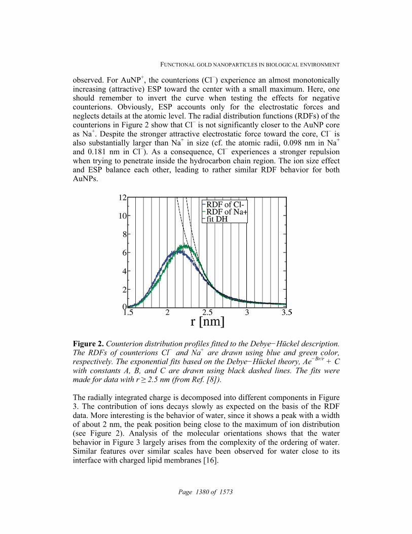
FUNCTIONAL GOLD NANOPARTICLES IN BIOLOGICAL ENVIRONMENT
observed. For AuNP+, the counterions (Cl−) experience an almost monotonically increasing (attractive) ESP toward the center with a small maximum. Here, one should remember to invert the curve when testing the effects for negative counterions. Obviously, ESP accounts only for the electrostatic forces and neglects details at the atomic level. The radial distribution functions (RDFs) of the counterions in Figure 2 show that Cl− is not significantly closer to the AuNP core as Na+. Despite the stronger attractive electrostatic force toward the core, Cl− is also substantially larger than Na+ in size (cf. the atomic radii, 0.098 nm in Na+ and 0.181 nm in Cl−). As a consequence, Cl− experiences a stronger repulsion when trying to penetrate inside the hydrocarbon chain region. The ion size effect and ESP balance each other, leading to rather similar RDF behavior for both AuNPs.
Figure 2. Counterion distribution profiles fitted to the Debye−Hückel description. The RDFs of counterions Cl− and Na+ are drawn using blue and green color, respectively. The exponential fits based on the Debye−Hückel theory, Ae−Br/r + C with constants A, B, and C are drawn using black dashed lines. The fits were made for data with r ≥ 2.5 nm (from Ref. [8]). The radially integrated charge is decomposed into different components in Figure 3. The contribution of ions decays slowly as expected on the basis of the RDF data. More interesting is the behavior of water, since it shows a peak with a width of about 2 nm, the peak position being close to the maximum of ion distribution (see Figure 2). Analysis of the molecular orientations shows that the water behavior in Figure 3 largely arises from the complexity of the ordering of water. Similar features over similar scales have been observed for water close to its interface with charged lipid membranes [16].
Page 1380 of 1573

FUNCTIONAL GOLD NANOPARTICLES IN BIOLOGICAL ENVIRONMENT
One of the exciting topics in electrolyte solutions concerns the distribution of ions around other charged objects. In the present case with counterions, the proper theoretical context is given by the (mean-field) Debye−Hückel (DH) theory, where for counterions around a charged particle, one combines the Poisson equation to specify the electrostatic potential of an ion with the Boltzmann equation for charge distribution. In radial symmetry, the Debye−Hückel description for the counterion distribution around a charged NP reads as Ae−Br/r + C, where A, B, and C are (positive) constants. Here, the constant C is included due to finite system size. However, the most relevant parameter for our purposes is 1/B = κ, known as the Debye screening length.
Figure 3. Radially integrated charge in AuNP solutions decomposed into the different components (from Ref. [8]). As our data for counterion distributions were fitted to the DH description, the agreement was found to be very good although the number of ions was limited to
Page 1381 of 1573

FUNCTIONAL GOLD NANOPARTICLES IN BIOLOGICAL ENVIRONMENT
60 to neutralize the functional groups of the AuNP. The contact life-times between ions and the AuNP are rapid, and the diffusion of ions is also fast, indicating that the statistics during the 200 ns simulations for the ion distributions are quite substantial. The deviations between the ion distribution data and the DH descriptions emerge around 2.4 nm from the AuNP center of mass, which can be considered as an approximate location for the interface (often called a double layer) between NP-bound and loosely associated counterions, the latter being able to move rather freely in the system despite the presence of the NP. The fits shown in Figure 2 yield values of 0.27 and 0.20 nm for the Debye length in AuNP+ and AuNP−, respectively. These lengths are 1 order of magnitude smaller than the NP size, which implies that the assumptions of the Smoluchowski theory for zeta potential determination are valid in the present case.
Figure 4. Zeta potential. ESPs of AuNP+ and AuNP– are drawn using black and red lines, respectively (from Ref. [8]). Let us assume that 2.4 nm is a safe (that is likely too large) estimate for the position of the interface between NP-bound and loosely bound ions. In this case, ESP gives an approximate estimate for the zeta potential: 26 mV for AuNP+ and −59 mV for AuNP−. The different numbers highlight that cationic and anionic AuNPs respond to an external field with different strengths. Further, even if our assumption of the location of the interface were partly inaccurate, we can still conclude that the zeta potential in the present systems without salt is about 25
Page 1382 of 1573

FUNCTIONAL GOLD NANOPARTICLES IN BIOLOGICAL ENVIRONMENT
mV, or larger than this value, which is often considered as a threshold value for coagulation/aggregation. Further, if there were salt, the Debye length would decrease for increasing ion concentration, which would show up as an increase in the zeta potential. Recent experimental data by Verma et al. for AuNPs protected by a number of different organic ligands is in agreement with this view, since they found the (absolute value of) zeta potential to vary between ∼31 and 38 mV [5]. Our analysis predicts that the AuNPs considered in this work do not coagulate.
4. Conclusions This article reviews our recent work on AuNPs in aqueous environment [8]. Our results highlight the importance of electrostatics and the nanoparticle−solvent interface in determining the properties of AuNPs. The results provide insight into the properties of charged and functionalized NPs in aqueous surroundings. Considering that the model used in this work is particularly realistic and is in agreement with a wide range of experiments, its predictions for AuNPs are expected to be highly useful in follow-up considerations of NP effects on biological systems. Our data show that NPs of this type cannot be considered as distinct bodies, but they form complexes together with the ions and solvent molecules surrounding them due to long-range interactions. This implies that in NP solutions there are interactions between the nanoparticles due to the ordering effects of water and ions around the NPs, which give rise to long-range solvent-mediated interactions that complement those due to hydrodynamics (conservation of momentum). The significance of these effects is stressed by the fact that nanomaterials in biological environments are rarely pristine neutral particles, as instead (synthetic) NPs under these conditions are usually charged or polar. The present results may therefore have generic interest especially in biological situations where synthetic nanomaterials interact with and aim to access cells. The main barrier that they need to overcome is the cell membrane characterized by a membrane potential coupled to a cloud of salt ions. Therefore, the central issue that is worth clarifying is the interaction between NP complexes and cell membranes. On the basis of our results, the characteristic length over which charged AuNPs may affect biological molecules or complexes (such as lipid membranes) in terms of water-mediated interactions is at least ∼10 nm. Depending on the NP charge and the molecular composition of the membrane, the reorganization of the lipid membrane system that results from this interplay is expected to vary. We continue our work on AuNPs in this direction.
Page 1383 of 1573

FUNCTIONAL GOLD NANOPARTICLES IN BIOLOGICAL ENVIRONMENT
References:
[1] M. DANIEL AND D. ASTRUC, Chem. Rev. 104 (2004) 293-346. [2] R. W. MURRAY, Chem. Rev. 104 (2008) 2688-2720. [3] M. WALTER, J. AKOLA, O. LOPEZ-ACEVEDO, P. JADZINSKY, G. CALERO,
C. ACKERSON, R. WHETTEN, H. GRÖNBECK, AND H. HÄKKINEN, Proc.Natl. Acad. Sci. U.S.A. 105 (2008), 9157−9162.
[4] O. LOPEZ-ACEVEDO, K.A. KACPRZAK, J. AKOLA, AND H. HÄKKINEN, Nat. Chem. 2010, 2, 329−334.
[5] A. VERMA, O. UZUN, Y. HU, Y. HU, H.-S. HAN, N. WATSON, S. CHEN, D.J. IRVINE, AND F. STELLACCI, Nat. Mater. 7 (2008), 588−595.
[6] P.R. LEROUEIL, S.A. BERRY, K. DUTHIE, G. HAN, V.M. ROTELLO, D.Q. MCNERNY, J.R. BAKER JR., B.G. ORR, AND M.M. BANASZAK HOLL, Nano Lett. 8 (2008), 420−424.
[7] R.R. ARVIZO, O.R. MIRANDA, M.A. THOMPSON, C.M. PABELICK, R. BHATTACHARYA, J.D. ROBERTSON, V.M. ROTELLO, Y.S. PRAKASH, AND P. MUKHERJEE, Nano Lett. 10 (2010), 2543−2548.
[8] E. HEIKKILA, A.A.GURTOVENKO, H. MARTINEZ-SEARA, H. HÄKKINEN, I. VATTULAINEN, AND J. AKOLA, J. Phys. Chem. C. 116 (2012), 9805-9815
[9] N. CHAKI, Y. NEGISHI, H. TSUNOYAMA, Y. SHICHIBU, AND T. TSUKUDA, J. Am. Chem. Soc. 130 (2008), 130, 8608−8610.
[10] J. AKOLA, M. WALTER, R. WHETTEN, H. HÄKKINEN, AND H. GRÖNBECK, J. Am. Chem. Soc. 130 (2008), 130, 3756−3757.
[11] O. LOPEZ-ACEVEDO, J. AKOLA, R. WHETTEN, H. GRÖNBECK, AND H. HÄKKINEN, J. Phys.Chem.C 113 (2009), 5035−5038.
[12] J.F. HICKS, D.T. MILES, AND R.W. MURRAY, J. Am. Chem. Soc. 124 (2002), 13322−13328.
[13] D. VAN DER SPOEL, E. LINDAHL, B. HESS, G. GROENHOF, A.E. MARK, AND H.J.C. BERENDSEN, J. Comput. Chem. 26 (2005), 1701−1718.
[14] H.J.C. BERENDSEN, D. VAN DER SPOEL, AND R. VAN DRUNEN, Comput. Phys. Commun. 91 (1995), 43−56.
[15] H. HEINZ, R.A. VAIA, B.L. FARMER, AND R.R. NAIK, J. Phys. Chem. B 112 (2008), 17281−17290.
[16] A.A. GURTOVENKO, M. PATRA, M. KARTTUNEN, AND I. VATTULAINEN, Biophys. J. 86 (2004), 3461−3472.
Page 1384 of 1573

Proceedings of the 12th International Conference on Computational and Mathematical Methods in Science and Engineering, CMMSE2012 La Manga, Spain, July, 2-5, 2012
A general purpose non-linear optimization framework based on Particle Swarm Optimization
J. Izquierdo1, I. Montalvo2, M. Herrera1 and R. Pérez-García1
1 FluIng-IMM, Universitat Politècnica de València, Valencia, Spain 2 3SConsult GmbH, Karlsruhe, Germany
emails: [email protected], [email protected],
[email protected], [email protected]
Abstract Classical methods of optimization show various limitations when dealing with many real-world engineering problems. Typically these problems are non-linear, large-scale combinatorial, non-convex, multi-objective optimization problem, involving various types of decision variables and many complex implicit constraints. In this paper we provide a synergetic association between swarm intelligence and multi-agent systems, which results in a powerful collaborative system for finding solutions to complex optimization problems. After showing its ability to find the global optimum for three well-known benchmark test functions, we consider the design of a real water distribution system, a truly complex problem with hundreds of dimensions. Key words: particle swarm optimization, optimal design, water distribution systems
1. Introduction Many real-world engineering problems can be cast as optimization problems (OPs). However, classical optimization methods (OMs) involve the use of gradients or higher-order derivatives of the fitness function, and are not well suited for many real-world problems since they are unable to deal with highly-dimensional, multimodal, and strongly non-linear problems; while, at the same time, are bound to process inaccurate, noisy, complex and mixed continuous-discrete data. As a consequence, in many fields of science and engineering, the OMs employed have conditioned the way in which real OPs have been
Page 1385 of 1573

NON-LINEAR OPTIMIZATION FRAMEWORK BASED ON PSO
approached. Consciously or unconsciously, problems have been adapted to the OMs in use. Robust OMs are often required to generate suitable results. Recently, many researchers have embarked on the implementation of various evolutionary algorithms (EAs). EAs are derivative-free global search algorithms able to obtain good solutions for various real-world OPs. In this paper we specifically refer to particle swarm optimization (PSO) [1], an EA based on swarm intelligence. A PSO-based environment has been developed by the authors [2] that takes ideas from a multi-agent philosophy, and crystallizes on a platform where different kinds of agents may interact and co-operate in the solution of a given OP [3-6]. First, we concisely describe a variant of PSO developed by the authors and endow it with a multi-agent (MA) approach. Then, the developed framework is tested with three well-known benchmark functions in the literature. Finally, we provide a succinct description of the various objectives and constraints involved in the water distribution network (WDN) optimal design problem, and provide the solution for two case studies, which consider real-world WDNs.
2. Swarm intelligence and MA approach for multi-objective OPs We describe a synergetic combination of swarm intelligence principles and MA system properties aimed at solving general multi-objective problems.
2.1 PSO approach In single-objective PSO a group of M particles are considered. The ith particle, Xi, is associated with its location in a d-dimensional subset, S Rd, where d is the number of problem variables. Any set of values of the d variables determines the particle location and represents a candidate solution for the optimization problem:
Find )(min XFSX
, subject to appropriate constraints,
where F is a scalar fitness function associated with the problem, a minimization problem without loss of generality. The optimal solution is then searched for by iteration starting from a random set of particles. The performance of each particle is measured using this fitness function, according to the problem in hand. During the process, each particle i is associated at each iteration, t, with three vectors:
its current position, Xi = (xi1… xid); its best so-far position, Yi = (yi1… yid) = argmin(F(Xi(t)), F(Xi(t-1))); and its flight velocity Vi = (vi1… vid), which makes it evolve.
The particle in the best position, Y* = argminF(Xi(t), i = 1,…, M, is identified for every iteration. At each generation, the velocity of each particle is updated in a
Page 1386 of 1573

NON-LINEAR OPTIMIZATION FRAMEWORK BASED ON PSO
process based on its recent trajectory, its best encountered position, the best position encountered by any particle, and a number of parameters:
Vi ← Vi + c1 rand( ) (Yi - Xi) + c2 rand( ) (Y* - Xi). (1)The parameters in (1) are as follows: is a factor of inertia suggested in [7] that controls the impact of the velocity history on the new velocity; c1 and c2 are two positive acceleration constants, called the cognitive and social parameters, respectively; rand( ) represents a function that creates random numbers between 0 and 1; two independent random numbers enter equation (1). In each dimension, velocities are clamped to minimum and maximum velocities,
Vmin Vij Vmax, (2)in order to control excessive roaming by particles outside the search space. They determine the resolution with which regions between the present position and the target (best so far) positions are searched. Usually, Vmin is taken as -Vmax. Finally, the position of each particle is updated every generation:
Xi ← Xi + Vi. (3)This is the standard PSO algorithm, which is applicable to continuous systems. The authors have endowed this algorithm with three new features that consider mixed variables, enriched diversity, and self-adapting parameters. Mixed variables. Several approaches have been put forward to tackle discrete problems with PSO. The approach we propose for discrete variables involves just the use of the integer part of the discrete velocity components. According to this simple idea, expression (1) will be replaced by
Vi ← fix(Vi + c1 rand( ) (Yi - Xi) + c2 rand( ) (Y* - Xi)), (4)for discrete variables, where fix() is a function that takes the integer part of its argument. Observe that the new velocity discrete values must be controlled by suitable bounds as in (2). In [4], it was found that using different velocity limits for discrete and continuous variables produces improved results. Enriched diversity. The main drawback of PSO is the difficulty in maintaining acceptable levels of population diversity while balancing local and global searches; and as a result, suboptimal solutions are prematurely obtained [8]. In general, the random character that is typical of evolutionary algorithms adds diversity to the manipulated populations. Yet, in PSO these random components are unable to add sufficient diversity and frequent collisions of particles in the search space, especially with the leader, Y*, can be detected – as shown in [5]. This causes the effective size of the population to fall, and the algorithm’s effectiveness is consequently impaired. In [9] a few of the best particles are checked for collisions; and colliding particles are randomly re-generated. This re-generation has been shown to avoid premature convergence as it prevents clone populations from dominating the search. The inclusion of this procedure into PSO
Page 1387 of 1573

NON-LINEAR OPTIMIZATION FRAMEWORK BASED ON PSO
increases diversity; as well as improves convergence characteristics and the quality of the final solutions.
Self-adaptive parameters. The role of in (1) and (4) is considered critical for the convergence behavior of the PSO algorithm. To ease the balancing of global and local searches, is usually allowed to adaptively decrease with time – it initially emphasizes global search, and then increasingly prioritizes local searches [10,11]. In contrast, we incorporate the acceleration coefficients and the clamping velocities into the optimization problem [6]. Each particle is allowed to self-adaptively set its own parameters by using the same process used by PSO – and given by expressions (1) or (4), and (3). To this end, these three parameters are considered as three new variables that are incorporated into the position vector Xi. In general, if d is the dimension of the problem, and p is the number of self-adapting parameters, the new position vector for particle i will be:
Xi = (xi1, …, xid, xid+1, …, xid+p). (5) These new variables do not enter the fitness function, but rather they are manipulated by using the same mixed individual-social learning paradigm used in PSO. Also, Vi and Yi increase their dimension, correspondingly. By using expressions (1) or (4), and (3), each particle is additionally endowed with the ability to self-adjust its parameters by taking into account the parameters it had at its best position in the past; as well as the parameters of the leader, which facilitated this best particle’s move to its privileged position.
2.2 Multi-objective PSO The emergent behavior of a PSO swarm is strongly reminiscent of the philosophy behind the multi-agent paradigm [12]. In an MA system each agent has a limited capacity and incomplete information to solve a problem – and therefore has a limited view of the solution. Each agent acting alone cannot solve the problem in its entirety, but a group of agents, with the coexistence of different views, is better able to find a solution by interacting together. This idea can be clearly extrapolated to the case of multi-objective optimization, since the result of the many interactions occurring within an MA system is improved performance. A departure from the standard behavior of particles in PSO was performed [2]. In addition to using the concept of Pareto dominance, various other aspects must also be re-stated. We then re-define the concept of leadership, adopt a normalization procedure, and propose two mechanisms to enrich the Pareto front. Leadership. The most natural option is to select as leader the closest particle to the so-called utopia point in the objective space. The utopia point is the point in the objective space with the best values for every objective. The utopia point is an unknown point since the best value for every objective is something unknown at the start (and perhaps during the whole process). Accordingly, we use a dynamic
Page 1388 of 1573

NON-LINEAR OPTIMIZATION FRAMEWORK BASED ON PSO
approximation of this utopia point, termed the singular point, which is updated with the best values found so far during the evolution of the algorithm [13]. Normalization. Since objectives are expressed in different units, regularisation for evaluating distances in the objective space is needed. Once a regularisation mechanism has been enforced, the Euclidean distance is used to establish the distance between any two objective vectors. Note that the worst and best objective values are updated while the solution space is explored. Pareto front enrichment. Arguably, the most interesting solutions are located near the singular point. Yet, unbalanced Pareto fronts may develop with respect to the singular point. Consequently, poorly detailed sections on the Pareto front may appear that may be worth exploring. It seems plausible that problem complexity is the cause of this asymmetry in many real-world, multi-objective OPs. It is not easy to find a general heuristic rule for deciding which parts of the Pareto front should be more closely represented. Those decisions are strongly dependent on the problem itself, and on the people solving the problem. In fact, additional information is always needed for making final decisions in the real-world [14]. This information can be established a priori, for example when objectives are represented in only one weighted expression. Additional information can also be used at the end for deciding which solution from a Pareto front should be selected. As a third possibility, additional information can be used during the search process; in our case this idea is implemented for deciding which regions of the Pareto front are worth exploring. We describe here one approach based on dynamic population increase to raise the Pareto front density, and another approach that adds swarms to complete poorly represented areas of the front. In the first approach, during the search process, swarms are able to increase their populations autonomously in order to better define the Pareto front: an agent whose solution belongs to the Pareto front may, on its evolution, find another solution belonging to the front. Then, a new clone of the agent is placed where the new solution is found, thus increasing the density of solutions on the Pareto front. In the second approach, the concept of a singular point is extended to any desired point in the objective space. This is performed by users, which are allowed to add new swarms for searching in desired regions of the objective space. The combination of various swarms within the same algorithm is efficient because it conducts a neighborhood search in which each of the swarms specializes, and the best improvement step in terms of Pareto optimality is followed to yield a new solution. The practice of incorporating different search mechanisms also reduces the probability of the search becoming trapped in local optima.
Page 1389 of 1573

NON-LINEAR OPTIMIZATION FRAMEWORK BASED ON PSO
3. Testing with three benchmarking functions Various nonlinear benchmark functions are commonly used in literature. We consider here three of them: the Griewark, Rastrigin and Rossenbrock functions with 30 variables are checked for optimization. These functions, their domains and their optima (zero for the three of them) can be found in [15]. The maximum number of generations is set to 2000 and the population size to 100. Populations are symmetrically initialized. The algorithm was executed in 50 independent runs. The mean fitness values of the best particle found for the 50 runs for the three functions, which slightly improve the results given in [15], are listed in Table 1.
Table 1. Mean optimum values for the three considered functions Function Rosenbrock Rastrigin Griewark
Mean values 0.12 2.43 0.0002
4. Testing with a real-world problem We briefly describe some of the objectives involved in the design of a WDN. Then, we show through two real case-studies that the described multi-objective model exhibits great robustness and good explanatory outcomes.
4.1 Problem definition Various objectives may be considered in the WDN optimal design problem. Cost of components Apart from the basic variables of the problem, which are the diameters of the new pipes, additional variables that depend on the design characteristics of the system may be required: storage volume, pump head, type of rehabilitation to be carried out for various parts of the network, etc. The correct approach to assess the costs for each element is important when defining the objective function, which has to be fully adapted to the problem under consideration in terms of design, enlargement, rehabilitation, operational design, etc. It is also important that the objective function reflects with utmost reliability the total cost of the system during its lifetime. For the sake of simplicity, we only consider here the cost related to the L pipes of the network, which includes the cost of new pipes, Lnew, and the cost of rehabilitated pipes, Lreh. This function, besides contributing most of the total cost, exhibits the characteristics we are interested in underlining. Costs corresponding to other elements, typically non-linear, are just new terms to be added within this fitness function (see [16], for example). The cost of the pipes is expressed as
L
iii lDcDC
1)()( , (6)
the sum extended to all individual pipes. D = (D1, …, DL)t is the vector of the pipe diameters. The costs per meter, depending on the diameter of pipe i, Di, is given
Page 1390 of 1573

NON-LINEAR OPTIMIZATION FRAMEWORK BASED ON PSO
by c(Di); li is the i-th pipe length. Note that Di is chosen from a discrete set of commercially available diameters, and c(.) is a non-linear function of diameter. There are various rehabilitation options: no rehabilitation, relining, duplication, and replacement are the most usual. Rehabilitation costs are also non-linear. Working conditions or scenarios The working conditions for a WDN depend on the values adopted by two types of variables, namely, demand models and roughness coefficient values. Typically, independent random variables are used to model both types of variables. Under the assumption that design is made to work for Ndm demand models and Nrc sets of roughness coefficient values, the design is performed for Nwc = NdmNrc
working conditions. These conditions have individual probabilities, kPwc , k = 1, …, Nwc, given by the product of the corresponding probabilities regarding demand models and roughness values. In the case of inclusion of the operational costs of the network along a certain temporal horizon, the necessary amortization rates must be considered. In this case, the objective cost function, omitting for simplicity the independent variables, may be represented by
k
k C Ca Ca C a CaPC OpertanktankvalvvalvpumppumppipepipewcNet . (7)
Values axxx correspond to amortization rates, Cpipe is given by expression (6), and the costs of pumps, tanks, valves, and operation (not detailed in this paper, as stated), are also considered. Observe that, in general, CNet is a non-linear, partially stochastic function depending on continuous, discrete, and binary variables. Hydraulic constraints Analyzing pressurized water systems is a mathematically complex task, especially for the large systems found in even medium-sized cities, since it involves solving many nonlinear simultaneous equations. Several formulations are available (see, for example, [17]). One formulation considers the N − 1 continuity equations, which are linear, plus the L energy equations, typically non-linear:
LkqqRHH
NiQq
kkkkk
iiNj
ij
,...,1
1,..,1,
21
. (8)
N is the number of demand junctions and L is the number of lines in the system. Ni is the number of nodes directly connected to node i; Qi is the demand associated to node i; k1 and k2 represents the end nodes of line k, which carries an unknown flowrate qk and is characterized by its resistance Rk, which depends on the diameter Dk and on qk through the Reynolds number (the non-linearity of the energy equations arises not only from the quadratic term, but also from the functions Rk = Rk(Dk,qk)). Hk1 and Hk2, piezometric heads at nodes k1 and k2, are unknown for consumption nodes and are given for fixed head nodes. The complete set of equations may be written, by using block matrix notation as
Page 1391 of 1573

NON-LINEAR OPTIMIZATION FRAMEWORK BASED ON PSO
Q
HA
H
q
A
AqA f10t12
1211
0
)(, (9)
where A12 is the connectivity matrix describing the way demand nodes are connected through the lines. Its size is L × Np, Np being the number of demand nodes; q is the vector of the flowrates through the lines; H the vector of unknown heads at demand nodes; A10 describes the way fixed head nodes are connected through the lines and is an L × Nf matrix, Nf being the number of fixed head nodes with known head Hf, and Q is the Np-dimensional vector of demands. Finally, A11(q) is an L × L diagonal matrix, with elements iiiiiii qABqRa / , (10)
with Ri being the line resistance, and Ai, Bi coefficients characterizing a potential pump. System (9) is a non-linear problem, whose solution is the state vector x = (qt, Ht)t (flowrates through the lines and heads at the demand nodes). Since most water systems involve a huge number of equations and unknowns, system (9) is usually solved using some gradient-like technique. We use EPANET2 [18], of widespread use around the world. Satisfaction of demand quality WDN design is typically performed subject to achieve an adequate service level, most of the times, a certain minimum pressure level at each node of the system. Other constraints include maximum pipe flow velocities and minimum concentrations of chlorine, for example. There are various ways of expressing lack of compliance with pressure, velocity, disinfectant, etc., conditions. For example, an objective function considering pressure and velocity constraints given by minimum values of node pressures and pipe velocities, may be given by
),()()()( min1
minmin1
min i
L
iij
N
jj vvvvHppppHP
(11)
where all the functions involved depend on D through the hydraulic model, and H is the step Heaviside function. Parameters and help normalize the impact of the different scales between pressure and velocity, and this enables a more meaningful aggregation of various types of constraint violation, and can also be used to balance the importance of one over the other. Extensions of (11) may be provided to consider maximum bounds and also additional objectives, such as limiting the level of chlorine in each pipe in the case of a water quality OP. Reliability and tolerance WDNs are almost always designed with loops so as to provide alternative, redundant paths from the source to every network node. This reduces the number of affected consumers when a pipe is withdrawn from service. Redundancy includes two important concepts: firstly, the connectivity necessary to provide alternative flow paths to each node; and secondly, the provision of an adequate
Page 1392 of 1573

NON-LINEAR OPTIMIZATION FRAMEWORK BASED ON PSO
flow capacity (diameter) for those paths [19]. The concept of redundancy is closely related to reliability [19, 20]. The concept of reliability was introduced to quantitatively measure the possibility of maintaining an adequate service for a given period. An explicit formulation of these concepts in probabilistic terms and their further integration implies considerable mathematical and algorithmic complexity. Thus, although numerous WDN reliability quantification schemes exist [19, 20], most are computationally expensive. As an example, a simple reliability formulation as in [17, 21] only considers pipe failures. Considering an average time for the duration of pipe failure, reliability R is defined as:
L
k k
knfreq pfqpf q
qR
10
1, (12)
where qreq is the total required network demand (the sum of all demands); qnf , the total flow delivered to the network when there are no failures; pf0 the probability of the whole network working without failure; qk the total flow delivered to the network when pipe k fails, and pfk is the failure probability of pipe k. Again, R is a function of D, the vector of diameters, through the hydraulic model.
4.2 Case studies and results The optimization problem may be addressed as a single or as a multi-objective problem. For a single objective approach an objective is selected, while others are introduced as ‘suitable’ penalty costs. For example, the following fitness function RPCDF )( , (13)
considers the piping costs, C, and penalty terms P, that considers the lack of compliance with some required minimum pressure level, and R, regarding the lack of reliability. and are ‘suitable’ penalty factors.
Figure 1. Sectors of a WDN in a Latin American capital and the design solutions
Page 1393 of 1573

NON-LINEAR OPTIMIZATION FRAMEWORK BASED ON PSO
A single objective problem One sector of the WDN of a Latin American capital (see the layout in Figure 1, left) is considered. This sector is fed by a tank (in red), and has 294 lines amounting to 18.337 km of pipe and 240 nodes consuming 81.53l/s in total. So, the dimension of the problem is 294. Figure 1 (left) also presents the solution obtained by using (13). Line colors represent pipe diameters. The formulation we consider here aims at minimizing the cost of a new network with the diameters of the pipes as design variables, while satisfying a minimum pressure in all the nodes and, at the same time, providing a certain amount of enforced reliability. The reliability scenarios considered here follow the approach of closing by turn all the pipes of a specific design to check if all the constraints are fulfilled by a design subjected to these circumstances. If the test is negative the design is penalized. In this way, designs will develop increasing reliability. To undergo those tests, the system must be analyzed for any of those specific ‘closures’. Only solutions assessed as being feasible by EPANET2 are considered. A multi-objective analysis We present the case-study of a different sector of the same WDN (Figure 1, right). The design involves the three objectives described above in a multi-objective solution: minimizing the investment cost, the lack of pressure at demand nodes, and the additional costs because of reliability problems. This network, also fed by a tank (blue box), has 132 lines and 104 consumption nodes; its total length being 9.055km, and the total consumed flowrate amounting to 47.09l/s. So, this three-objective problem is 132-dimensional. In Figure 2 a bi-dimensional (cost against lack of pressure) representation of the approximated Pareto front that considers the three mentioned objectives is presented. Two swarms can be identified (blue and red points) that build the three-dimensional Pareto front of this problem. Observe that the representation is a projection in two dimensions of points in the real Pareto front, which is a surface in a three-dimensional space.
Figure 2. Approximated Pareto front for a real-world network
Lack of pressure. Lima sector.
Cost $
Page 1394 of 1573

NON-LINEAR OPTIMIZATION FRAMEWORK BASED ON PSO
Plenty of enriched information that helps the decision-making process is provided by this type of representation of the Pareto front. For example, it becomes evident, as expected, that after some point, the rate at which the minimum pressure can be increased in the network is much lower than the rate at which initial investment costs must be increased to achieve the desired pressure level.
5. Conclusions The development of a multi-objective optimization framework enables the combination of economic, engineering, and policy viewpoints when searching for a solution to a problem. For example, the relationship between the initial investment cost and the minimum pressure in the network may help decide, among other factors, which pressure would be better to use for the final solution. In this case (in which there is a limited budget to implement the design) the decision-maker has at his or her disposal a clear guideline to assess how much the quality may be improved if the budget is increased by a certain amount. This is an added value of the multi-objective approach when solving the problem of optimal design of WDNs. Decision makers are thus provided with a set of informed solutions to select the best design with regard, for example, to available resources and/or other criteria. Acknowledgments Thanks to the support of the project IDAWAS, DPI2009-11591, of the Dirección General de Investigación of the Ministerio de Educación y Ciencia, and ACOMP/2010/146 of the Conselleria d‘Educació of the Generalitat Valenciana. References:
[1] J. KENNEDY AND R. C. EBERHART, Particle swarm optimization, Proc. of the IEEE International Conf. on Neural Networks, Piscataway, NJ, (1995), 1942-1948.
[2] I. MONTALVO, Optimal Design of Water Distribution Systems Using Agent Swarm Optimization, Doctoral dissertation. Universitat Politècnica de València, Valencia, Spain, 2011.
[3] I. MONTALVO, J. IZQUIERDO, R. PÉREZ AND M. M. TUNG, Particle Swarm Optimization applied to the design of water supply systems, Comput. Math. Appl. 56(3) (2007) 769–776.
[4] J. IZQUIERDO, I. MONTALVO, R. PÉREZ AND V. S. FUERTES, Design optimization of wastewater collection networks by PSO, Comput. Math. Appl. 56(3) (2007) 777–784.
[5] I. MONTALVO, J. IZQUIERDO, R. PÉREZ, R. AND P. L. IGLESIAS, A diversity-enriched variant of discrete PSO applied to the design of Water Distribution Networks, Eng. Optimiz. 40(7) (2008) 655-668.
[6] I. MONTALVO, J. IZQUIERDO, R. PÉREZ AND M. HERRERA, Improved performance of PSO with self-adaptive parameters for computing the
Page 1395 of 1573

NON-LINEAR OPTIMIZATION FRAMEWORK BASED ON PSO
optimal design of Water Supply Systems, Eng. Appl. Artif. Intel. 23(5) (2010) 727-735.
[7] Y. F. SHI AND R. C. EBERHART, A modified particle swarm optimizer, IEEE Int. Conf. Evol. Comp. (1998) 69–73.
[8] Y. DONG, B. X. J. TANG AND D. WANG, An application of swarm optimization to nonlinear programming, Comput. Math. Appl. 49(11-12) (2005) 1655–1668.
[9] M. HERRERA, J. IZQUIERDO, I. MONTALVO AND R. PÉREZ-GARCÍA. Injecting diversity into particle swarm optimization. Application to water distribution system design, Adv. Comp. Sci. Eng. 6(2) (2011) 159-179.
[10] Y. F. SHI AND R. C. EBERHART, Empirical study of particle swarm optimization, Proc. IEEE Congr. Evol. Comp. (1999) Washington DC.
[11] Y. X. JIN, H. Z. CHENG, J. I. YAN AND L. ZHANG, New discrete method for particle swarm optimization and its application in transmission network expansion planning, Electr. Pow. Syst. Res. 77(3-4) (2007) 227-233.
[12] M. WOOLDRIDGE, An Introduction to Multiagent Systems, John Wiley & Sons, 2002.
[13] I. MONTALVO, J. IZQUIERDO, S. SCHWARZE AND R. PÉREZ-GARCÍA, Multi-objective particle swarm optimization applied to water distribution systems design: An approach with human interaction, Math. Comput. Model. 52 (2010) 1219-1227.
[14] C.A. COELLO-COELLO, G.B. LAMONT AND D.A. VAN VELDHUIZEN, Evolutionary Algorithms for Solving Multi-Objective Problems, Springer, 2007.
[15] Y. JIANG, F. HU, C. HUANG, W. XIANING, An improved particle swarm optimization algorithm, Appl. Math. Comput. 193 (2007) 231-239.
[16] A. S. MATÍAS, Diseño de redes de distribución de agua contemplando la fiabilidad, mediante algoritmos genéticos, Ph.D. thesis, Universitat Politècnica de València, Valencia, Spain, 2003.
[17] J. IZQUIERDO, R. PÉREZ AND P. L. IGLESIAS, Mathematical models and methods in the water industry, Math. Comput. Model. 39 (2004) 1353–1374.
[18] L. A. ROSSMAN, EPANET 2 User's Manual, Cincinati (IN), Environmental Protection Agency, 2000.
[19] J. B. MARTÍNEZ, Cost and reliability comparison between branched and looped water supply networks, J. Hydroinform. 12(2) (2010) 150-160.
[20] I. C. GOULTER, T. M. WALSKI, L. W. MAYS, A. B. A. SEKARYA, R. BOUCHART AND Y K. TUNG, Reliability analysis for design, in: Water distribution systems handbook, L.W. Mays, ed., McGraw-Hill, New York, 2000.
[21] P. KALUNGI AND T. T. TANYIMBOH, Redundancy model for water distribution systems, Reliab. Eng. Syst. Safe. 82(3) (2003) 275-286.
Page 1396 of 1573

Proceedings of the 12th International Conference on Computational and Mathematical Methods in Science and Engineering, CMMSE2012 La Manga, Spain, July, 2-5, 2012
Quantum-chemical studies of organic molecular crystals –
structure and spectroscopy
Christoph R. Jacob1 and Ralf Tonner
2
1 Center for Functional Nanostructures, Karlsruhe Institute of Technology (KIT) ,
Wolfgang-Gaede-Str. 1a, 76131 Karlsruhe, Germany 2 Fachbereich Chemie and Materials Sciences Center, Philipps-Universität
Marburg, Hans-Meerwein-Straße, 35043 Marburg, Germany
email: [email protected], [email protected]
Abstract
Organic molecular crystals are of current interest because of their
optoelectronic properties. Structural and spectroscopic properties can be
analysed with density-functional theory (DFT) based methods given that
dispersion interactions are taking into account. Single-molecule, cluster, and
crystal approaches are compared here and a mode-localization procedure is
applied. In this presentation, perfluoropentacene is investigated in detail and
other organic crystals are presented as well.
Key words: Density-functional theory, dispersion interactions, molecular
crystals, computational spectroscopy, mode localization
1. Introduction
Molecular crystals play a major role in the field of organic electronics mostly due to their
optoelectronic properties. Theoretical modelling of these properties thus necessitates an
accurate description of the molecular structure and packing in these crystals. Results from
computations can on the one hand be validated by comparison of structural data to results
from X-ray or neutron diffraction data or on the other hand to spectroscopic properties. In
particular, simulation of infrared (IR) measurements is of interest here since it is one of the
most common spectroscopic techniques in material science.
Density-functional theory (DFT) has become the preferred method for ab initio-investigations
of solid state materials and surfaces in the last decades.[1] Intriguingly, this is so despite the
well-known shortcoming of present-day exchange-correlation (XC) functionals with respect
to the description of long-range dispersion interactions.[2] Empirically, these non-covalent
interactions can be understood as the attractive part of the van der Waals (vdW) potential
between moieties not directly bonded to each other.[3] The main reason for this failure has
been identified in the wrong long-range behaviour of current XC-functionals and several
approaches have been developed to correct for this error.[3-4] It was concluded that a proper
description of dispersion interactions is not only necessary for molecular systems but also for
condensed matter and especially for non-covalently bound molecular crystals due to the
known overestimation of lattice parameters associated with GGA functionals.[5]
Page 1397 of 1573

QUANTUM-CHEMICAL STUDIES OF ORGANIC MOLECULAR CRYSTALS
For the investigation of realistic systems with large unit cells semiempirical approaches like
the a posteriori dispersion-correction scheme by Grimme (DFT-D)[6] or Tkatchenko and
Scheffler[7] were developed. These schemes add atomic pairwise correction terms to the DFT
energy based on dispersion coefficients for atoms and derive the correct long-range behaviour
of these interactions. The DFT-D scheme will be applied here to derive accurate structures of
the molecular crystals under investigation.
The simulation of spectroscopic data is usually carried out in the single-molecule
approximation. Alternatively, cluster calculations can be performed to simulate the crystal
environment in a non-periodic approach. Computed spectra for clusters can then be analysed
and related to single-molecule calculations with the help of an analysis in terms of localized
modes.[8] This can help in identifying the scope and limitations of this approach.
2. Methods
Molecules and Cluster
Geometry optimizations without symmetry constraints have been carried out for the
molecules using the Gaussian09 optimizer[9] in combination with Turbomole6[10] energies
and gradients. Several density functionals (PBE, BP86 and B3LYP) were employed as well as
an ab initio method (MP2) together with the def2-suite of basis sets (SVP, TZVPP and
QZVPP) developed by Weigend et al[11] applying the resolution of identity approximation.
Harmonic vibrational spectra were derived by calculating the Hessian matrix analytically.
Analysis of the vibrational spectra of the PFP7-cluster model was carried out with the aid of a
recently described localization procedure.[8]
Molecular Crystals
This part of the study employed the Vienna Ab Initio Simulation Package (VASP 5.2)[12]
applying periodic boundary conditions (PBC). Several density functionals were tested for
their performance. The projector-augmented wave (PAW) method[13] was used. Structural
optimization was performed starting from the experimental crystal structures by means of a
conjugate-gradient or quasi-Newton algorithm for ionic positions and cell parameters.
Harmonic vibrational frequencies at the -point of the molecular crystal were calculated
through building up the force constant matrix in a density-functional perturbation theory
(DFPT) approach. IR intensities were calculated with an approach originally formulated by
Giannozzi and Baroni as implemented in VASP for the PAW formalism.[14] More details can
be found in Ref. [15].
Dispersion effects have been considered by the scheme proposed by Grimme in the D2
formulation[6a] as implemented in VASP[5b] and the more recent D3 formulation.[16]
3. Results
Structural and spectroscopic properties of perfluoropentacene (PFP) were investigated in a
single-molecule approximation, a cluster approach, and by employing the periodicity of the
molecular crystal. As shown in Fig. 1, the agreement between experiment and theory for the
IR spectrum is very good. Especially the observed vibrational Davydov splittings (i.e. the
splittings of vibrational bands in a crystal due to the occurrence of more than one molecule in
the unit cell) can be described based on the computations.[15]
Page 1398 of 1573

QUANTUM-CHEMICAL STUDIES OF ORGANIC MOLECULAR CRYSTALS
Table 1. Experimental (single crystal x-ray[17]) and computed structural
parameters (in degrees and Å) and unit cell volume (V) for molecular crystal of PFP
with and without dispersion correction.
a b c V V[a]
Exp. 15.51
(1)
4.490
(4)
11.449
(11) 90
91.567
(13) 90
797.0
(13)
PBE-D3 15.564 4.431 11.506 90 91.122 90 793.4 -0.5%
PBE-D2 15.546 4.356 11.352 90 91.490 90 768.4 -3.6%
PBE 15.678 4.727 11.927 90 90.416 90 883.9 +10.9% rPBE-D3 15.648 4.453 11.581 90 91.084 90 806.8 +1.3%
[a] deviation from experimental volume
The focus in the present study is on the comparison of the three computational approaches
towards structural details and spectroscopic signatures. While the molecular structure of the
PFP molecule is reproduced by different methods with an accuracy of approx. 0.01 Å (RMS
w.r.t. X-ray data), the reproduction of the lattice parameters proves to be more difficult. As
can be seen in Table 2, the GGA functional (PBE) overestimates the unit cell volume by
approximately 10% which is a general phenomenon in non-covalently bound crystals.[5a]
Only the addition of a dispersion correction scheme gives the correct bulk structure with
subtle differences for the different approximations.
Figure 1 IR-spectrum of PFP from experiment (black), single-
molecule approximation (PBE/def2-TZVPP, blue) and molecular
crystal calculation (PBE-D2, red).[15]
In between the single-molecule approximation and the calculation of spectra for the molecular
crystal is the possibility to employ a cluster approach. To this end, a PFP7-cluster was
optimized and the vibrational spectrum analysed. The inherent mode coupling leads to a
complicated spectrum which is hard to analyse in detail (Fig. 2a). Employing a localization
procedure, we could analyse the effect of the non-periodic surrounding on the vibrational
spectrum of the central molecule (Fig. 2b). This method makes it possible to separate the
direct effect of the surrounding molecules on the molecular vibrations from the coupling of
the vibrations on different molecules (i.e. Davydov splittings).
Page 1399 of 1573

QUANTUM-CHEMICAL STUDIES OF ORGANIC MOLECULAR CRYSTALS
In this contribution, the structural and spectroscopic details of the investigations for PFP will
be highlighted within the single-molecule approximation, a molecular cluster and employing
the full crystal surrounding. Further work will include structural and energetic investigations
of another example of molecular semiconductors (NTCDA = 1,4,5,8-Naphthalene-
tetracarboxylic dianhydride) and a hydrogen-bonded crystal (-(trifluoromethyl)-lactic
acid).[18]
2. Acknowledgments
We thank the experimental collaborators on the PFP project T. Breuer, P. Jakob and G. Witte
(Marburg) as well as M. Celik (Stuttgart) for initial work on the subject.
3. References
[1] J. HAFNER, Ab-initio simulations of materials using VASP: Density-functional theory
and beyond, J. Comput. Chem. 29, (2008) 2044-2078.
[2] A. GROSS, Theoretical Surface Science - A Microscopic Perspective; Springer
Verlag: Berlin, Heidelberg, 2009.
[3] S. S, Density functional theory with London dispersion corrections, WIREs Comput.
Mol. Sci. 1, (2011) 211-228.
[4] A. TKATCHENKO, L. ROMANER, O. T. HOFMANN, E. ZOJER, C. AMBROSCH-
DRAXL, M. SCHEFFLER, Van der Waals Interactions Between Organic Adsorbates
and at Organic/Inorganic Interfaces, MRS Bull. 35, (2010) 435-442.
[5] a) T. TODOROVA, B. DELLEY, Molecular Crystals: A Test System for Weak
Bonding, J. Phys. Chem. C 114, (2010) 20523-20530; b) T. BUČKO, J. HAFNER, S.
LEBEGUE, J. G. ANGYÁN, Improved Description of the Structure of Molecular and
Layered Crystals: Ab Initio DFT Calculations with van der Waals Corrections, J.
Phys. Chem. A 114, (2010) 11814-11824.
[6] a) S. GRIMME, Semiempirical GGA-type density functional constructed with a long-
range dispersion correction, J. Comput. Chem. 27, (2006) 1787-1799; b) S.
GRIMME, J. ANTONY, S. EHRLICH, H. KRIEG, A consistent and accurate ab
initio parametrization of density functional dispersion correction (DFT-D) for the 94
elements H-Pu, J. Chem. Phys. 132, (2010) 154104.
[7] A. TKATCHENKO, M. SCHEFFLER, Accurate Molecular Van Der Waals
Interactions from Ground-State Electron Density and Free-Atom Reference Data,
Phys. Rev. Lett. 102, (2009) 073005.
Figure 2. Normal-mode spectrum (left) and modes localized on central molecule (right) for PFP7-cluster (BP86-D2/def2-
SVP)(middle).
Page 1400 of 1573

QUANTUM-CHEMICAL STUDIES OF ORGANIC MOLECULAR CRYSTALS
[8] a) C. R. JACOB, M. REIHER, Localizing normal modes in large molecules, J. Chem.
Phys. 130, (2009) 084106; b) C. R. JACOB, S. LUBER, M. REIHER, Analysis of
Secondary Structure Effects on the IR and Raman Spectra of Polypeptides in Terms of
Localized Vibrations, J. Phys. Chem. B 113, (2009) 6558-6573.
[9] M. J. FRISCH, G. W. TRUCKS, H. B. SCHLEGEL, G. E. SCUSERIA, J. A. POPLE,
et al., Gaussian Inc., Gaussian 09, Revision C.01, Wallingford CT, 2009.
[10] R. AHLRICHS, M. BÄR, M. HÄSER, H. HORN, C. KÖLMEL, Electronic structure
calculations on workstation computers: the program system TURBOMOLE, Chem.
Phys. Lett. 162, (1989) 165-169.
[11] F. WEIGEND, R. AHLRICHS, Balanced basis sets of split valence, triple zeta
valence and quadruple zeta valence quality for H to Rn: Design and assessment of
accuracy, Phys. Chem. Chem. Phys. 7, (2005) 3297-3305.
[12] G. KRESSE, J. FURTHMÜLLER, Efficient iterative schemes for ab initio total-
energy calculations using a plane-wave basis set, Phys. Rev. B 54, (1996) 11169-
11186.
[13] a) P. E. BLÖCHL, Projector augmented-wave method, Phys. Rev. B 50, (1994)
17953-17979; b) G. KRESSE, D. JOUBERT, From ultrasoft pseudopotentials to the
projector augmented-wave method, Phys. Rev. B 59, (1999) 1758-1775.
[14] M. GAJDOS, K. HUMMER, G. KRESSE, J. FURTHMÜLLER, F. BECHSTEDT,
Linear optical properties in the projector-augmented wave methodology, Phys. Rev. B
73, (2006) 045112.
[15] T. BREUER, M. CELIK, P. JAKOB, R. TONNER, G. WITTE, Vibrational Davydov-
Splittings and Collective Mode Polarizations in Oriented Organic Semiconductor
Crystals, J. Phys. Chem. C, (2012) submitted.
[16] J. MOELLMANN, S. EHRLICH, R. TONNER, S. GRIMME, A DFT-D Study of
Structural and Energetic Properties of TiO2 modifications, J. Phys.: Condens. Matter,
(2012) in print.
[17] Y. SAKAMOTO, T. SUZUKI, M. KOBAYASHI, Y. GAO, Y. FUKAI, Y. INOUE, F.
SATO, S. TOKITO, Perfluoropentacene: High-performance p-n junctions and
complementary circuits with pentacene, J. Am. Chem. Soc. 126, (2004) 8138-8140.
[18] R. TONNER, V. A. SOLOSHONOK, P. SCHWERDTFEGER, Theoretical
investigations into the enantiomeric and racemic forms of -(trifluoromethyl)lactic
acid, Phys. Chem. Chem. Phys. 13, (2011) 811-817.
Page 1401 of 1573

Proceedings of the 12th International Conference on Computational and Mathematical Methods in Science and Engineering, CMMSE2012 La Manga, Spain, July, 2-5, 2012
Computational study of solids irradiated by intense x-ray free-electron lasers
Hikaru Kitamura
Department of Physics, Kyoto University, Kyoto 606-8502, Japan
email: [email protected]
Abstract Quantum-chemical and statistical methods to simulate elementary processes in solids interacting with an intense x-ray free-electron laser (XFEL) pulse are presented. Cluster-model calculations reveal that multiple core holes created through photoexcitation can modify the entire electronic structure of the system considerably. The cluster model is combined with the density-matrix equation to analyze femtosecond dynamics of electronic excitation, collisional relaxation, and photoabsorption edge shifts. We also mention solid-state energy-band calculations of photoabsorption coefficients for a simple metal over a wide range of photon energies. Key words: XFEL, photoabsorption, core-electron excitation
1. Introduction X-ray free-electron laser (XFEL) [1-3], a new light source producing intense and coherent x-rays with femtosecond pulse duration, is becoming available for experiments to probe microscopic structures and ultrafast dynamics in atoms, molecules, clusters and bulk materials. It is of considerable significance to elucidate microscopic interactions of solids with an intense XFEL pulse by means of quantum-statistical theories and computer simulations. The XFEL pulse is intense and its photon energy can be tuned at the excitation energy of a particular inner-shell; we may thus excite many core electrons resonantly, realizing a nonequilibrium solid that contains multiple core holes and extra conduction electrons. The lifetime of a core hole may be limited mainly by the Auger decay [4] and the radiative decay [5], where the latter may be prevalent
Page 1402 of 1573

SOLIDS IRRADIATED BY INTENSE XFEL
in heavier elements [6]. The electrons excited to the conduction band undergo relaxation through scattering with the other conduction electrons [7]. Excess kinetic energies of the electrons can also be transferred to ions through electron-phonon coupling [8], which might eventually lead to a destruction of the crystalline order. This paper presents recent developments of quantum-statistical methods to simulate those elementary processes in simple metallic solids interacting with an XFEL pulse.
2. Cluster model To begin with, we investigate how the electronic structure of a solid is modified when many core electrons are simultaneously excited to the conduction band. For this purpose, quantum-chemical electronic-structure calculations in the unrestricted Hartree-Fock (UHF) approximation have been performed for a model Li9 cluster arranged in a body-centered cubic (bcc) configuration [9].
−0.6−0.5−0.4−0.3−0.2−0.1
0
0 5 10 15 20 25 30 35−3.8−3.6−3.4−3.2
−3−2.8−2.6−2.4
ρ(ε) (states/hartree/atom)
ε (h
artre
e)
Li9 DOS, ground state
HOMO = −0.123
−0.6−0.5−0.4−0.3−0.2−0.1
0
0 5 10 15 20 25 30 35−3.8−3.6−3.4−3.2
−3−2.8−2.6−2.4
ρ(ε) (states/hartree/atom)
ε (h
artre
e)
Li9 DOS, hollow−atom state
HOMO = −0.262
FIGURE 1: Density of states for a Li9 cluster in the ground state (left panel) and a neutral K-shell excited state with one 9 core holes (right panel). In Figure 1, the electronic density of states () for the ground state is compared with that for a neutral excited state with one core hole per atom. It can be observed that the entire energy levels are lowered as a result of excitation, which implies that the core holes localized at each atomic site produce strong attractive fields to the surrounding electrons. It turns out that the core levels (shown in
Page 1403 of 1573

SOLIDS IRRADIATED BY INTENSE XFEL
lower panels) are lowered more drastically than the valence levels (upper panels), leading to an enhancement of the core-valence energy gap [9,10]; it gives rise to a blue shift of the K-edge that we shall demonstrate in Sec. 3.2.
3. Density-matrix equation To compute dynamics of electrons in the presence of a laser field, we combine the UHF cluster calculation is with the density-matrix equation [11,12] as follows: (i) One-electron wave functions ( )k r and the corresponding energies k
are computed through the UHF equations without a laser field. Here, k and refer to an index of one-electron states and spin, respectively. (ii) Electronic transitions between a set of states k and k’ after an onset of the laser pulse are computed through the Heisenberg equation of motion for the one-electron density matrix, †
kk kkc c , as
,kkkki H
t
. (1)
Here, †
kc and kc refer to the creation and annihilation operators of an electron in state (k,), denotes an expectation value; H is a total Hamiltonian, which is a sum of the UHF Hamiltonian, the electron-electron interaction term beyond and UHF approximation, and the electron-laser interaction term. Dynamical shifts of energy levels can also be analyzed through Eq. (1). We note that it is impossible to solve Eq. (1) exactly, because the electron-electron interaction term in H produces a two-electron density matrix 1 1 2 1 3
† †k k k kc c c c ,
which in turn depends on higher-order density matrices [12]. A crude way of truncating such a hierarchy of correlation is the Born approximation with exchange [11,12], which is adopted in this work. We remark, however, that validity of such an approximation is not ensured for core-level excitation where electron-hole correlation is strong.
3.1. Energy-level shift An onset of photoexcitation gives rise to a creation of core holes and hence the orbital energy ( )k t may deviate from the initial ground-state value k
. Analysis of Eq. (1) within the UHF approximation yields [11]
Page 1404 of 1573

SOLIDS IRRADIATED BY INTENSE XFEL
11 1 1 1 1 11 1
1 1
occ( ) ( )k k kk k k k kkkk kk
t V V f t
. (2)
Here,
1 2 1 1 2 21 2 3 4 1 2 3 4
2* *
1 2 1 1 2 21 2
( ) ( ) ( ) ( )k k k k k k k ke
V d d r r r r r r
r r (3)
is the Coulomb matrix element, k kkf represents the population of state
(k,); occ 1k if state (k, ) is occupied in the ground state and occ 0k otherwise. Test calculation for a lithium dimer illustrated in Fig. 2 indicates that Eq. (2) may produce approximate orbital energies in a core-excited state without solving the UHF equations explicitly. In a bulk metal, additional contribution from electron screening to the energy-level shift should be considered [10] through the correlation part of the two-electron density matrix.
−10
−8
−6
−4
−2
−110−100−90−80−70−60−50
α β α β
Li (1s22s) Li*(1s2s2)
numerical ( )model ( )
ε k (e
V)
∼
1s
2s
FIGURE 2: Orbital energies of a Li2 molecule in 1s22s ground state and 1s2s2 excited state. The solid lines represent numerical solutions to the UHF equations; the dotted lines are approximate results obtained through Eq. (2). The symbols and designate up-spin and down-spin states, respectively.
3.2. Rate equation So far as the time scale of population change is slower than that of the oscillating laser field, we may invoke the Markov approximation; Eq. (1) can thus be reduced to a rate equation [11],
abs emi
( )
( ) ( ; ) ( ; ) ( ) ( )kkk kk k k
k k
f t It t f t f t
t
Page 1405 of 1573

SOLIDS IRRADIATED BY INTENSE XFEL
in out1 ( ) ( )
( ) ( )k k
k k
f t f t
t t
. (4)
Here, I and denote the intensity and the frequency, respectively, of the laser pulse. The time-resolved photoabsorption cross-section associated with transition of an electron from initial state k’ to final state k is given as
22
abs2 2 2e
( )4( ; )3 ( ( ))
kkkk
kk
et
c m t
p
, (5)
where me refers to the electron mass, ( )kk
p represents the matrix element of the
electron momentum operator, ( )kk t denotes the excitation energy between the initial and final states including their energy-level shifts, and is a phenomenological parameter accounting for energy-level broadening. Similar expression can be obtained for the emission cross-section, emi ( ; )kk t . The
quantities in ( )k t and out ( )k t are incoming and outgoing rates, respectively, of an electron in state (k, ) due to collisional processes such as the Auger decay and intraband collision. Figure 3 illustrates a change of photoabsorption K-edge spectra of lithium irradiated by a laser pulse with = 60 eV, I = 1014 W/cm2, and the pulse width of 40 fs. Numerical results have been obtained through solutions to Eq. (4) for a model Li24 cluster through the UHF method with the aid of the NDDO (neglect of diatomic differential overlap) approximation [11]. The photoabsorption coefficient has been evaluated in accordance with Eq. (5) as
absatomabs ( ; ) ( ; ) ( ) ( )kk k k
kk
nt t f t f t
N
(6)
with N (= 24) being the cluster size; natom denotes the atomic density in the solid. It can be observed that the position of the K-edge shifts to high-energy side, leading to a reduction of abs() at = . The edge shift is a consequence of the enhancement of the band gap associated with photoexcitation; about 12% of 1s electrons have been excited to the conduction band in this example. Such an absorption saturation leads to ultrafast switching of an FEL pulse passing through the target [13], which was demonstrated through N-shell excitation of a Sn target by Yoneda et al. [14] using a vacuum ultra-violet (VUV) FEL .
Page 1406 of 1573

SOLIDS IRRADIATED BY INTENSE XFEL
In the cluster model, the number of atoms is finite so that the resultant one-electron energy spectrum may become too sparse to reproduce the observed energy bands or photoabsorption spectra of real solids [15]. In the next section, we shall present an alternative approach based on the solid-state theory.
50 60 70 800
0.5
1
1.5
2
2.5
0
1
2
3
4
5
6
hω (eV)
κ abs
(ω)/n
atom
(10−1
8 cm2 /a
tom
)
−
t=40fs
t=0
experiment(arbitrary units)
FIGURE 3: Photoabsorption cross-section of lithium excited by a laser pulse with = 60 eV and I = 1014 W/cm2. The dotted curve represents the initial spectrum; the solid curve is the spectrum at 40 fs after an onset of the laser pulse. The dashed curve depicts the experimental spectrum in the ground state by Haensel et al. [15] in arbitrary units (right axis).
4. Solid-state band calculation We have recently performed electronic band-structure calculations of photoabsorption cross-sections of Na metal in the ground state for photon energies of 20-2000 eV. The conduction-band wavefunctions n,k(r), characterized by wave vector k and band index n, have been expanded in terms of the orthogonalized plane waves (OPWs) OPW ( )k+G r , with G denoting the reciprocal lattice vector [16]. Since an x-ray can excite an electron to an energy on the order of keV, the cut-off value of G has been set as large as 11.8 au (i.e., 2G2/2me = 1890 eV). The core-electron wavefunctions have been approximated by the published Hartree-Fock data for isolated atoms [17], neglecting overlap of neighboring cores. The one-electron potential has been evaluated approximately by summing up the electron-screened Hartree potentials of ion cores and exchange energies of uniform electron gas. The wavefunctions have been
Page 1407 of 1573

SOLIDS IRRADIATED BY INTENSE XFEL
sampled at 84 k-points in the irreducible Brillouin zone with the aid of the tetrahedral method [18,19].
102 10310−3
10−2
10−1
100
101
hω (eV)
cros
s−se
ctio
n (1
0 −18 cm
2 /ato
m)
−
NIST
NOPW=1
FIGURE 4: Photoabsorption cross-sections of Na metal. The solid curve is the result of the full band calculation; the dotted curve is the corresponding result in the single-OPW approximation. The dot-dashed curve represents NIST database [20]. Photoabsorption cross-sections can be computed through equations analogous to (5) and (6), where index k is now replaced by k, n. Preliminary results are displayed in Fig. 4 for a photon energy above the LII,III-edge. For a comparison, the corresponding result in the single-OPW approximation, OPW( ) ( )k kr r , is indicated. We find that the cross-section in the single-OPW approximation agrees well with the NIST database [20] for an energy range of about 200-1000 eV, but it predicts a spurious dip in the spectrum above the K-edge ( 1200-1500 eV), as already pointed out separately in atomic physics [21]. As the size of the OPW basis increases, the dip tends to be diminished, whereas the cross-section below the K-edge turns out to be reduced. Moreover, the entire spectrum exhibits rapid oscillations due to a discontinuity of the band structure at the Brillouin-zone edge. Current databases on x-ray absorption spectra of solids [20,22] are compilations of existing experimental data and theoretical atomic photoionization cross-sections, where solid-state effects are ignored in the latter. Solid-state approach to x-ray spectra of simple metals was reported previously [23], but it focused mainly on the shape of the spectra close to the absorption edge, where electron-hole many-body correlations come into play. Systematic solid-state calculations
Page 1408 of 1573

SOLIDS IRRADIATED BY INTENSE XFEL
of absolute photoabsorption cross-sections over a wide range of photon energies are necessary to check the consistency with the existing databases.
5. Concluding remarks Cluster-model electronic-structure calculations and density-matrix equations have been presented to simulate electronic structures and femtosecond dynamics in multiple core-level photoexcitation of solids. Numerical results have been demonstrated for lithium irradiated by VUV FEL. It has been shown that strongly localized core holes can induce rapid shifts of energy levels and absorption saturation, with possible applications to nonlinear photonics. In order to extend those calculations to heavier elements and higher photon energies, solid-state band-structure calculations of absolute x-ray absorption cross-sections for simple metals are under way; preliminary results for Na solid have been presented.
Acknowledgments The author is grateful to Dr. H. Yoneda for pertinent discussions. This work was supported in part by a Grant-in-Aid for Promotion of Utilization of X-Ray Free-Electron Lasers and Grant-in-Aid for Scientific Research, provided by the Japanese Ministry of Education, Culture, Sports, Science and Technology. References:
[1] M. YABASHI AND T. ISHIKAWA eds., XFEL/SPring-8 Beamline Technical Design Report Ver. 2.0, RIKEN/JASRI, 2010.
[2] J. ARTHUR et al., Linac Coherent Light Source (LCLS) Conceptual Design Report, SLAC-R593, Stanford, 2002.
[3] M. ALTARELLI et al. eds., The European X-Ray Free-Electron Laser Technical Design Report, DESY 2006-097, 2007.
[4] V.O. KOSTROUN, M.H. CHEN AND B. CRASEMANN, Atomic Radiationless Transition Probabilities to the 1s State and Theoretical K-Shell Fluorescence Yields, Phys. Rev. A 3 (1971) 533-545.
[5] J.H. SCOFIELD, Radiative Decay Rates of Vacancies in the K and L Shells, Phys. Rev. 179 (1969) 9-16.
[6] A. KOTANI AND Y. TOYOZAWA, Theoretical Aspects of Inner-Level Spectroscopy, in Synchrotron Radiation, ed. C. Kunz, Springer-Verlag, Berlin (1979) 169-229.
Page 1409 of 1573

SOLIDS IRRADIATED BY INTENSE XFEL
[7] P.M. ECHENIQUE, J.M. PITARKE, E.V. CHULKOV AND A. RUBIO, Theory of inelastic lifetimes of low-energy electrons in metals, Chem. Phys. 251 (2000) 1-35.
[8] A.P. HORSFIELD, D.R. BOWLER, H. NESS, C.G. SÁNCHEZ, T.N. TODOROV AND A.J. FISHER, The transfer of energy between electrons and ions in solids, Rep. Prog. Phys. 69 (2006) 1195-1234.
[9] H. KITAMURA, Multiple K-shell excitation of lithium clusters: Implications for hollow-atom solids, Chem. Phys. Lett. 475 (2009) 227-231.
[10] H. KITAMURA, Band-gap enhancement in core-excited metals, Europhys. Lett. 94 (2011) 27005 (6pp).
[11] H. KITAMURA, Rate equation for intense core-level photoexcitation and relaxation in metals, J. Phys. B: At. Mol. Opt. Phys. 43 (2010) 115601 (10pp).
[12] F. ROSSI AND T. KUHN, Theory of ultrafast phenomena in photoexcited semiconductors, Rev. Mod. Phys. 74 (2002) 895-950.
[13] H. KITAMURA, Rapid energy-level shifts in metals under intense inner-shell photoexcitation, High Ene. Dens. Phys. 8 (2012) 66-70.
[14] H. YONEDA, Y. INUBUSHI, T. TANAKA, Y. YAMAGUCHI, F. SATO, S. MORIMOTO, T. KUMAGAI, M. NAGASONO, A. HIGASHIYA, M. YABASHI, T. ISHIKAWA, H. OHASHI, H. KIMURA, H. KITAMURA AND R. KODAMA, Ultra-fast switching of light by absorption saturation in vacuum ultra-violet region, Opt. Express 17, (2009) 23443-23448.
[15] R. HAENSEL, G. KEITEL, B. SONNTAG, C. KUNZ AND P. SCHEREIBER, Photoabsorption Measurement of Li, Be, Na, Mg, and Al in the XUV Range, Phys. Stat. Sol. A2 (1970) 85-90.
[16] T.O. WOODRUFF, The Orthogonalized Plane-Wave Method, Sol. State Phys. 4 (1957) 367-411.
[17] E. CLEMENTI AND C. ROETTI, Roothaan-Hartree-Fock Atomic Wavefunctions: Basis Functions and Their Coefficients for Ground and Certain Excited States of Neutral and Ionized Atoms, Z54, At. Data Nucl. Data Tables 14 (1974) 177-478 .
[18] D. ZAHARIOUDAKIS, Tetrahedron methods for Brillouin zone integration, Comp. Phys. Comm. 157 (2004) 17-31.
[19] G. LEHMANN AND M. TAUT, On the Numerical Calculation of the Density of States and Related Properties, Phys. Stat. Sol. (b) 54 (1972) 469-477.
[20] C.T. CHANTLER, Theiretical Form Factor, Attenuation and Scattering Tabulation for Z = 1-92 from E = 1-10 eV to E = 0.4-1.0 MeV, J. Phys. Chem. Ref. Data 24 (1995) 71-184.
[21] R.S. WILLIAMS AND D.A. SHIRLEY, Comparison of final state approximations in the calculation of total and differential photoemission cross sections of neon, J. Chem. Phys. 66 (1977) 2378-2386.
Page 1410 of 1573

SOLIDS IRRADIATED BY INTENSE XFEL
[22] B.L. HENKE, E.M. GULLIKSON AND J.C. DAVIS, X-Ray Interactions: Photoabsorption, Scattering, Transmission, and Reflection at E = 50-30000 eV, Z = 1-92, At. Data Nucl. Data Tables 54 (1993) 181-342.
[23] P.H. CITRIN, G.K. WERTHEIM AND M. SCHLÜTER, One-electron and many-body effects in x-ray absorption and emission edges of Li, Na, Mg, and Al metals, Phys. Rev. B 20 (1979) 3067-3114.
Page 1411 of 1573

Proceedings of the 12th International Conference on Computational and Mathematical Methods in Science and Engineering, CMMSE2012 La Manga, Spain, July, 2-5, 2012
Computational Methods for Problems of Viscoelastic Solid Deformation with Application to the Diagnosis of Coronary Heart
Disease
Carola Kruse, Matthias Maischak, Simon Shaw, John Whiteman¹,S
Greenwald, M Brewin², M Birch³, HT Banks, Z Kenz, S Hu 4 ¹BICOM, Brunel University, UK
²Blizard Institute, Barts and The London School of Medicine and Dentistry, Queen Mary, University of London, UK
³Clinical Physics, Barts and the London National Health Service Trust, UK 4 Center for Research into Scientific Computation, North Carolina State
University, USA Emails: [email protected], [email protected],
[email protected], [email protected]
Many solid materials, including much human tissue, deform viscoelastically. This talk will begin with a review of models for viscoelastic deformation and their discretisation using finite element techniques, developed by the BICOM group and collaborators in recent years. A major problem, for people in developed countries, but increasingly also elsewhere, is that of coronary heart disease (CHD) due to the presence of stenosis in coronary arteries. As plaque builds up in a coronary artery blood flow past the stenosed region becomes turbulent and creates abnormal variations in wall shear stresses. These shears drive low amplitude acoustic shear waves through the soft tissue in the thorax which appear at the chest wall and can be measured non-invasively by placing sensors on the skin. This acoustic surface signature has the potential to provide a cheap non-invasive means of diagnosing CHD. An interdisciplinary project exploiting the use of computational modelling in the diagnosis of CHD is in an initial stage. In this biomedical physicists are building cylindrical chest phantoms from tissue mimicking (viscoelastic) agarose gel which will simulate the process described above in a wet lab environment. In parallel, dry lab forward and inverse solver software is being built with the ultimate aim of being able to localize the stenosis in silico. The wet lab results will be used to provide input parameters to the software as well as, at a later stage, to validate it.
Page 1412 of 1573

VISCOELASTIC SOLID DEFORMATION
Axial symmetry of the phantom is being exploited for this first stage of the modelling. This talk describes the construction of the forward solver in the resulting 2D axial cross section. For this we consider a two-dimensional space-time ‘viscodynamic’ problem using a wave equation incorporating Zener (also known as a ‘standard linear solid’ or ‘Maxwell solid’) and Kelvin-Voigt models for viscoelasticity. We use a high order spectral finite element method in space and high order discontinuous Galerkin finite element discretization in time using normalized antiderivatives of Legendre polynomials. This choice allows the decoupling of the linear system following the technique of [T Werder et al., Comp Meth Appl Mech Engr 190: 6685 – 6708, 2001]. We present results illustrating the effect of this with respect to accuracy and convergence.
Page 1413 of 1573

Proceedings of the 12th International Conference on Computational and Mathematical Methods in Science and Engineering, CMMSE2012 La Manga, Spain, July, 2-5, 2012
Modeling Earthen Dikes: Sensitivity Analysis and Calibration of Soil Properties Based on Sensor Data
V.V. Krzhizhanovskaya1,2, N.B. Melnikova1,2
1 National Research University ITMO, Russia 2 University of Amsterdam, The Netherlands
emails: [email protected]
Abstract
A mathematical model of earthen dike behavior under dynamic hydraulic load describes a coupled fluid-structure interaction system. Transient flow through porous media is modeled by Richards equation with Van Genuchten model for water retention in partially saturated soil around the phreatic surface. Structural stability analysis is based on Drucker-Prager elastic perfectly plastic material model. We show the results of sensitivity analysis of porous flow dynamics to soil permeability; and calibration of soil properties based on sensor data from a real sea dike. Key words: dike, stability, flow in porous media, Richards equation, sensitivity analysis, calibration, soil permeability MSC2000: 76S05
1 Introduction Regular floods pose a serious threat to human life, valuable property and city infrastructure. Many international projects are aimed at the development of flood protection systems [1], including the UrbanFlood European project [2] that unites the work on monitoring dikes with sensor techniques [3], physical study of dike failure mechanisms [4], and software development for dike stability analysis [5], [6], simulation of dike breaching, flood, and city evacuation [7], [8], [9]. Most of the flood defenses are based on earthen dikes and levees. Their stability is of utmost importance for flood prevention. One of the goals of the UrbanFlood project was the development of the Virtual Dike computational model for
Page 1414 of 1573

MODELING DIKES: SENSITIVITY ANALYSIS AND CALIBRATION BASED ON SENSOR DATA
advanced research into dike stability and failure mechanisms [6], and for training the artificial intelligence module on simulated dike instabilities [5]. In numerical analysis of stability of an earthen dike under dynamically changing hydraulic loads, water pressure inside the dike contributes to the total stresses in the dike. The dynamics of pore pressure can provide important engineering information on the safety of the dike. Abnormal distribution of pore pressures may indicate the onset of dike macro-instability or piping. Sea tides or changing river levels influence the position of phreatic surface. Moving water table creates the zones with partially saturated soils. Resistance of porous media to the flow is modeled by Darcy’s law suitable for low velocities [10]. A problem of unconfined porous flow dynamics can be modelled either by Darcy’s equation on a moving mesh, adjusting the domain boundary position to coincide with the surface of zero pore pressure [11], or by using stationary mesh and solving Richards equation with non-linear rheological properties of the media depending on the effective water content. These non-linear properties can be modeled by classical models of Van Genuchten [13] or Brookes and Corey model [14], as well as by some approximations [12] simplified for faster numerical convergence. In this work we used Richards equation with Van Genuchten model, in order to perform simulations on a fixed mesh. A real dike is a heterogeneous porous media with unknown distribution of soil parameters. This paper presents numerical analysis of sensitivity of the porous flow simulation to the variation of soil permeability. Calibration of soil properties for the tidal groundwater flow is often performed by tidal method [15], [16], based on one-dimensional analytical models of half-infinite or finite aquifers. The method is suitable for aquifers with low elevation of phreatic surface with respect to the average depth. A more accurate way that works well for high amplitude of water level variation is direct numerical simulation. In present work, both analytical and numerical approaches have been tested and compared. Sensitivity analysis and calibration of soil properties have been performed for the LiveDike, a sea dike in Groningen, the Netherlands, equipped with a number of pore pressure sensors installed in four cross-sections (Figure 1). The height of the dike is 9 m, the width is about 60 m, the length is about 300 m. The remainder of this paper is organized as follows: Section 2 describes the mathematical model of dike behavior under dynamic hydraulic load; Section 3 gives model implementation details; Section 4 presents the results of sensitivity analysis and calibration of soil properties; and Section 5 concludes the paper.
Page 1415 of 1573

V.V. KRZHIZHANOVSKAYA, N.B. MELNIKOVA
Figure 1. (a) Location of the LiveDike, sea dike near Groningen, The Netherlands;
(b) LiveDike cross-sections with marked sensor locations
2 Mathematical model of dike behavior under hydraulic load Dike stability analysis requires solving a coupled fluid-structure interaction problem that was described in detail in [6]. Due to the page limit, here we describe only the fluid sub-model. It calculates the contribution of water pressure inside the dike to the total load calculated in the structural dynamics sub-model. The problem of flow through porous media is described by the pressure-based form of Richards equation [10], taking into account wetting and drying of the area above phreatic surface:
tgypkK
tpSC r
Se ∂
∂−=+∇−⋅∇+∂∂+ ερ
μθ )]([)( , (1)
where C=∂θ/∂p is specific moisture capacity, [1/Pa]; eθ = eθ (p) is effective water content; S is storage coefficient, [1/Pa]; p is gauge pressure (relative to atmospheric pressure), [Pa]; t is time, [s]; KS is permeability of saturated media, [m2]; kr=kr(p) is relative permeability of unsaturated soil; μ is dynamic viscosity of water, [Pa·s]; g is standard gravity, [m/s2]; ρ is water density [kg/m3]; y is a coordinate in vertical direction, [m]. The right-hand-side term t∂∂ε is a rate of volume deformation of soil skeleton, calculated by the structural sub-model. In this study, we assume that soil skeleton does not undergo large volume deformations during tidal load and therefore the RHS term is zero. This assumption makes our model one-way coupled, with an independent fluid sub-model.
(b)(a)
Page 1416 of 1573

MODELING DIKES: SENSITIVITY ANALYSIS AND CALIBRATION BASED ON SENSOR DATA
In saturated soil C=0, eθ =1, kr=1, and p≥0. In unsaturated zone, pressures are negative and properties of unsaturated soil (specific moisture capacity and relative permeability) are defined by van Genuchten equations as follows [13]:
0,0,0
)1()(1
/1/1
<⎪⎩
⎪⎨⎧
≥
−−−= p
pm
amC
mm
em
ers θθθθ , (2)
[ ]⎪⎩
⎪⎨⎧
≥<−−=
0,10,)1(1
2/1
ppk
mme
le
rθθ , (3)
where sθ is saturated water content; rθ is residual water content; and eθ is effective water content calculated by
⎪⎪⎩
⎪⎪⎨
⎧
≥
<⎥⎥⎦
⎤
⎢⎢⎣
⎡⎟⎟⎠
⎞⎜⎜⎝
⎛ −+=
−
0,1
0,1
p
pgp
mn
e ραθ , (4)
a, n, m=1-1/n, l are Van Genuchten parameters specific for each type of soil.
Equation (1) with soil properties defined by (2)-(4) is solved with boundary conditions of two possible types: pressure specified at the boundary S1 or normal flow velocity specified at the boundary S2:
sSpp =
1, )]([
2gypkKnV rSSn ρ+∇−⋅= , (5)
where n is a vector normal to the boundary surface. On impermeable walls Vn=0; for rainfall infiltration Vn=Vn(t).
3 Model implementation
3.1. Computational domain and boundary conditions Simulation domain represents a cross-section of the dike (Figure 2a). Boundary conditions for the flow sub-model are the following: At the sea side of the dike (black line on the left of Figure 2a), sea tides are modeled by a harmonic function for pressure dynamics:
])sin([ ythgp amp −⋅= ωρ , (6)
Page 1417 of 1573

V.V. KRZHIZHANOVSKAYA, N.B. MELNIKOVA where amph = 1.5 m is the amplitude of tidal oscillation of sea water level;
T/2πω = is radial frequency of the tidal cycle; tidal period T = 12 hr 25 min; y [m] is a vertical coordinate (y=0 is a reference water level). At the land side of the dike (cyan line on the right of Figure 2a) water level stays at the "NAP" level, a reference sea level in the Netherlands:
gyp ρ−= . (7)
Zero flux boundary condition 0/ =∂∂ np is imposed at the remaining boundaries (magenta lines in Figure 2a).
Figure 2. (a) Simulation domain and boundary conditions. "NAP" is a reference
sea level in the Netherlands (corresponds to y=0). (b) Finite element mesh with refinement area around the phreatic line.
3.2. Computational mesh and implementation details Partial differential equations (1) are solved by the finite element method: the computational domain is discretized into finite elements and original equations are reduced to a system of ordinary differential equations solved by implicit time integration scheme. We used the six-node triangular finite elements with second-order approximation. The mesh was refined in the zone around the phreatic line (see Figure 2b), where flow parameter gradients can be very high. Convergence of the finite element solution on a number of meshes with increasing density and higher order of approximation has been tested. The coarsest mesh that provided the error of less than 0.01% was chosen: 15000 elements of second order approximation. Computational time strongly depends on the amount of non-linearities in the model. The van Genuchten model for unsaturated soil is highly non-linear, and
(a) (b)
Page 1418 of 1573

MODELING DIKES: SENSITIVITY ANALYSIS AND CALIBRATION BASED ON SENSOR DATA
this fact significantly affects the rate of convergence for load regimes with zone saturation and drainage. For a period of 1 day (24 hours), porous flow simulation takes up to 1 hour. Convergence rate can be increased by choosing a less non-linear approximation of water retention curve. Structural sub-model takes about 10 minutes to simulate tidal oscillations of 1 day physical time. Memory demand does not exceed 1 Gb for a 2D problem.
4 Simulation results
4.1. Sensitivity analysis Sensitivity analysis has been performed to study the influence of soil permeability on pore pressure dynamics. Two main parameters can be identified to characterize the dike response to the tidal water load:
1. amplitude of pore pressure oscillations and 2. phase shift between the tidal load and pore pressure oscillations.
2D homogeneous computational domain has been considered. Geometric prototype of the domain is a LiveDike cross-section. The boundary conditions have been described in Section 3: harmonic tidal pressure head (eq. 6) is applied at the seaside; and constant pressure head (eq. 7) is applied at the landside. A number of porous flow simulations have been performed, with values of saturated permeability Ks in the range of 10-7-10-11 m2. Storage coefficient S was constant and equal to 10-7 Pa-1. Distribution of pore pressure amplitudes in a horizontal slice of the dike (at the level y = -6 m) is presented in Figure 3a. For relatively high values of permeability (K = 10-7 ÷ 10-9 m2) pressure amplitude is linear (like in 1D analytical models), with a very small non-linear tail close to the sea-side (left) slope. Non-linear part corresponds to the zone where the flow is
0
0.1
0.2
0.3
0.4
0.5
0.6
0.7
0.8
0.9
1
-30 10 50 90
x
pres
sure
am
plitu
de, P
a
K1E-7K1E-8K1E-9K1E-10K1E-11
1
10
100
1000
-30 10 50 90
x
phas
e sh
ift, m
in
Figure 3. (a) pressure amplitude distribution along the dike.
(b) phase shift distribution along the dike (in logarithmic scale). Data shown in a horizontal slice y = -6 m.
(a) (b)
Page 1419 of 1573

V.V. KRZHIZHANOVSKAYA, N.B. MELNIKOVA essentially 2D and can not be considered one-dimensional: at x<=10 m, water inlet is located both at the vertical boundary and on the under-water slope of the dike (see Figure 2a). At x>=10 m the flow can be treated as one-dimensional, and pressure amplitude distribution corresponds to the analytical solution (not shown in the paper due to the page limit). For permeability K=10-10 m2 and lower, significant non-linearity appears. The analytical model also predicts non-linear profiles of pressure distribution, however the absolute values of pore pressure do not agree with the finite element simulation. For example at K=10-10 m2 analytical pressure amplitude in point x=50 m is 0.5 Pa, while simulated amplitude is 0.2 Pa. Real pore pressure amplitude measured by the sensor "E4" located at x=50 m (see Figure 5) is 0.25 Pa. This corresponds to the permeability value K = 3·10-10 m2 (Figure 4a). Figure 3a clearly shows that pressure amplitude for highly permeable media (like (coarse sands) is insensitive to the actual value of permeability (lines for K=10-7, K=10-8 K=10-9 coincide). The distribution is defined only by the boundary conditions. To the contrary, the phase shift is sensitive to the value of permeability (Figure 3b), therefore phase shift can be calibrated by choosing appropriate Ks to match sensor data: Phase shift between the tide and real sensor "E4" is 30 min, which corresponds to the permeability value Ks = 10-9 m2 (see Figure 4b). Calibration of the LiveDike soil parameters based on this sensitivity analysis is described in the following subsection.
0
0.1
0.2
0.3
0.4
1.00E-111.00E-101.00E-091.00E-081.00E-07
permeability, m**2
rela
tive
pres
sure
am
plitu
de
0
50
100
150
200
250
1.00E-111.00E-101.00E-091.00E-081.00E-07
permeability, m**2
phas
e de
lay,
min
utes
Figure 4. Influence of soil permeability on (a) pressure amplitude and (b) phase
shift in sensor location (50m; -6m)
4.2. Calibration of soil properties The most informative sensor in the LiveDike is "E4" located in saturated zone (coordinates x=50 m, y=-6 m), see Figure 5, Figure 6. In addition, there are two more pressure sensors located in saturated zone: "E3" (also at x=50 m) and "G2" (x=72 m). E3 pressure oscillations are in phase with E4, with relative pressure amplitude 20% from tidal amplitude. G2 relative pressure amplitude is only 7%
(b)(a)
Page 1420 of 1573

MODELING DIKES: SENSITIVITY ANALYSIS AND CALIBRATION BASED ON SENSOR DATA
and that indicates that G2 is installed in a zone with low permeability. The distance between G2 and E3 is only 12 m, but pressure amplitude drops significantly. G2 sensor data allows to locate the outlet vertical boundary of simulation domain close to G2, and to specify a constant water level at zero meters from average sea level.
Figure 5. Cross-section of the LiveDike with sensors shown
-150.0
-50.0
50.0
150.0
28.08.2010 0:00 28.08.2010 12:00 29.08.2010 0:00
540565590615640
28.08.2010 0:00 28.08.2010 12:00 29.08.2010 0:00
265
270
275
280
28.08.2010 0:00 28.08.2010 12:00 29.08.2010 0:00
Figure 6. Top: Tidal sea level measured in LiveDike. Middle: pore pressure dynamics from sensor "E4" (x=50 m). Bottom: pore pressure dynamics from sensor "G2" (x=72 m).
Sea
tides
, cm
Pr
essu
re h
ead,
cm
Pr
essu
re h
ead,
cm
G2
E4
sea
Page 1421 of 1573

V.V. KRZHIZHANOVSKAYA, N.B. MELNIKOVA Pressure amplitude in E4 sensor has been calibrated by tuning appropriate location of the outlet boundary (x=70 m), where specified water table is zero meters from reference level. Phase shift for E4 has been calibrated by choosing Ks=0.9·10-9 m2 and S=10-7 Pa-1 in the zone x<=50 m between the sea and the sensor. The simulation results then perfectly match real sensor data, both for the "training" period shown in Figure 7a and for a long-term simulation shown in Figure 7b. For x>50 m soil parameters were found to be Ks=10-12 m2, S=10-7 Pa-1 to provide low pressure amplitude in sensor G2.
500
520
540
560
580
600
620
640
660
680
27.08.2010 22:12 28.08.2010 10:12 28.08.2010 22:12
pres
sure
hea
d, m
m
1E4 virtualE4
Figure 7. Pore pressure dynamics in sensor E4 with calibrated soil properties.
(a) comparison of real sensor data (light green) with simulation results (black) for a "training period"; (b) the same, for a period of 16 days.
5 Conclusions and future work A mathematical model of earthen dike behavior under dynamic hydraulic load has been developed. Transient flow through porous media was modeled by Richards equation with Van Genuchten model for water retention in partially saturated soil. Sensitivity analysis of porous flow dynamics to soil permeability showed that:
(a)
(b)
Page 1422 of 1573

MODELING DIKES: SENSITIVITY ANALYSIS AND CALIBRATION BASED ON SENSOR DATA
1. Distribution of pore pressure amplitudes across the dike (in horizontal direction from the sea) is close to linear for highly permeable soils (like coarse sands) and is significantly non-linear for non-permeable soils, such as clays.
2. Pressure amplitude for coarse media (Ks~10-9÷10-7 m2 and S=10-7 Pa-1) is insensitive to the value of permeability, and is defined only by boundary conditions.
3. The phase shift is always sensitive to the value of permeability and can be calibrated by choosing appropriate saturated permeability to match sensor data.
4. The results of analytical one-dimensional model qualitatively agree to the finite element simulation results, but the actual parameter values differ.
Soil properties have been calibrated based on the sensor data from a real sea dike. Simulation results with calibrated soil parameters match well experimental data, not only on the "training set" but also for a much longer period of time. This calibrated and validated model is now being integrated in the UrbanFlood early warning system, where the simulation can be run with a real-time input from water level sensors or with predicted high water levels due to the upcoming storm surge or river flood. In the first case, comparison of simulated pore pressures with real data can indicate a change in soil properties or in dike operational conditions (e.g. failure of a drainage pump). In the second case, simulation can predict the structural stability of the dike and indicate the "weak" spots in the dikes that require attention of dike managers and city authorities.
Acknowledgements This work is supported by the EU FP7 project UrbanFlood, grant N 248767; by the Leading Scientist Program of the Russian Federation, contract 11.G34.31.0019; and by the BiG Grid project BG-020-10, # 2010/01550/NCF with financial support from the Netherlands Organisation for Scientific Research NWO. It is carried out in collaboration with AlertSolutions, Deltares, IJkDijk Association, Rijkswaterstaat, Ministerie van Verkeer en Waterstaat, SARA Computing and Networking Services, UvA IBED-CGE, UvA GIS Studio, WaterNet, Waterschap Noorderzijlvest.
References [1] V.V. Krzhizhanovskaya et al. Flood early warning system: design,
implementation and computational modules. Procedia Computer Science, V. 4, pp. 106-115, 2011. http://dx.doi.org/10.1016/j.procs.2011.04.012
[2] UrbanFlood European Seventh Framework Programme project http://www.urbanflood.eu
Page 1423 of 1573

V.V. KRZHIZHANOVSKAYA, N.B. MELNIKOVA [3] A.L. Pyayt et al. Machine Learning Methods for Environmental Monitoring
and Flood Protection. World Academy of Science, Engineering and Technology, Issue 78, pp. 118-124, June 2011. http://www.waset.org/journals/waset/v78/v78-23.pdf
[4] IjkDijk project http://www.ijkdijk.eu [5] A.L. Pyayt et al. Artificial Intelligence and Finite Element Modelling for
Monitoring Flood Defence Structures. Proc. 2011 IEEE Workshop on Environmental, Energy, and Structural Monitoring Systems. Milan, Italy, September 2011, pp. 1-7 http://dx.doi.org/10.1109/EESMS.2011.6067047
[6] N.B. Melnikova, G.S. Shirshov, V.V. Krzhizhanovskaya. Virtual Dike: multiscale simulation of dike stability. Procedia Computer Science, V. 4, pp. 791-800, 2011. http://dx.doi.org/10.1016/j.procs.2011.04.084
[7] N.B. Melnikova et al. Virtual Dike and Flood Simulator: Parallel distributed computing for flood early warning systems. Proc. International Conference on Parallel Computational Technologies (PAVT-2011). Publ. Centre of the South Ural State University, Chelyabinsk, pp. 365-373. http://omega.sp.susu.ac.ru/books/conference/PaVT2011/short/139.pdf
[8] B. Gouldby, V.V. Krzhizhanovskaya, J. Simm. Multiscale modelling in real-time flood forecasting systems: From sand grain to dike failure and inundation. Procedia Computer Science, V. 1, p. 809. http://dx.doi.org/10.1016/j.procs.2010.04.087
[9] A. Mordvintsev, V.V. Krzhizhanovskaya, M. Lees, P.M.A. Sloot. Simulation of City Evacuation Coupled to Flood Dynamics. Proc. of the 6th
International Conference on Pedestrian and Evacuation Dynamics, PED2012. ETH Zurich. 6-8 June 2012 (In print)
[10] J. Bear. Hydraulics of Groundwater, McGraw-Hill, 1979 [11] Gordon A. Fenton, D. V. Griffiths. A mesh deformation algorithm for free
surface problems. International Journal for Numerical and Analytical Methods in Geomechanics. V. 21, Issue 12, pp. 817–824, December 1997.
[12] K.-J. Bathe et al. Finite element free surface seepage analysis without mesh iteration. International Journal for Numerical and Analytical Methods in Geomechanics. V. 3, Issue 1, pp. 13–22, January/March 1979
[13] M.T. van Genuchten. A closed form equation for predicting the hydraulic conductivity of unsaturated soils. Soil Science Society of America Journal, 44: 892-898, 1980
[14] R.H. Brooks, A.T. Corey. Properties of porous media affecting fluid flow, J. Irrig. Drainage Div., ASCE Proc, V. 72 (IR2), pp. 61–88, 1966
[15] A.J. Smith, W.P. Hick. Hydrogeology and aquifer tidal propagation in Cockburn Sound, Western Australia. CSIRO Land and Water. Technical report 6/01. February 2001
[16] J. A. Williams. R. N. Wada. R.-Y. Wang. Model studies of tidal effects on ground water hydraulics. Project Completion Report. 1970
Page 1424 of 1573

Proceedings of the 12th International Conference on Computational and Mathematical Methods in Science and Engineering, CMMSE2012 La Manga, Spain, July, 2-5, 2012
Modeling of the Charge Density for Long and Short
Channel Double Gate MOSFET Transistor
S.Latreche1 and B.Smali
1
1Laboratoire Hyperfréquence & Semi-conducteur (LHS),
Département d’Electronique, Faculté des Sciences de l’Ingénieur,
Université Mentouri Constantine, 25000, Algérie
emails: [email protected], [email protected].
Abstract
In this paper, we present a numerical method to compute the
mobile charge density for long and short channel model of a
Double Gate MOSFET transistor. In the first time, a brief
description of the compact model for long and short channel
device is presented, and the static behavior of the DG MOSFET
is obtained using a relationship between charges and voltages.
The model is based on the formalism EKV developed for the
MOSFET bulk. In second time, to define the explicit solution of
the gate charge density in weak and strong inversion, we use the
Taylor series development. From that, we get an efficient
algorithm that computes the gate/mobile charge density with a
faster computation time, without any iterative procedure and it is
valid for both cases of the transistor. Our results are compared
with the iterative calculation using the Newton-Raphson
method, and especially compared with 2-D numerical
simulations using ATLAS-TCAD software.
Key words: DG MOSFET, Short channel, long channel, EKV
model, Taylor series development, charge density, circuit
simulation.
1. Introduction
In the last few years, the CMOS technology has approached the limit caused by
the quantum and physical effects appears in nanoscale devices [1]. As a solution
to this problem, different architectures were developed: the undoped DG
MOSFET architecture is one of the best candidates for the future integrated
circuits. This structure can offer many advantages such as: an ideal 60 mV/decade
Page 1425 of 1573

COMPUTING THE CHARGE DENSITY OF THE DG MOSFET
subthreshold slope, reduced short channel effects (SCEs), free dopant associated
fluctuation effects [2], [3].
Compact modeling of nanoscale devices is important to describe the relation
between the physical process, geometry and the electrical behavior, especially
important for circuits design applications [4].
Some compact models of the DG MOSFET structure have been presented in the
literature [5, 6, 7]. However, most of them are good for the physical device but
less useful for circuit simulation, because these models are built on complicated
analytical expressions or implicit solutions that need to be numerically solved,
generally an iterative calculation.
In this work, we present a numerical procedure to compute the gate/mobile charge
density for long and short channel model of the DG MOSFET transistor.
In the first part, from 1-D Poisson’s equation of the long channel undoped DG
MOSFET we get a relationship between charges and voltages. The short channel
model is derived from the 2-D Poisson’s equation and the parabolic potential
approximation.
However, the fundamental equation of the model needs an iterative procedure to
calculate the mobile charge density, but this is not suitable for circuit simulation.
In the second part, by applying the Taylor series development in the fundamental
equation of the model in weak and strong inversion, we find a polynomial
equation. From the solution of this polynomial equation, the explicit solution of
the gate charge density in weak and strong inversion is obtained. An efficient
algorithm that computes the mobile/gate charge density without any iterative
calculation and without any problem of time convergence is defined.
Finally, our results obtained using MATLAB environnement are compared with
2-D numerical simulation obtained by Silvaco-ATLAS software. We also achieve
a comparison with the Newton-Raphson method, applying to the fundamental
equation of the model.
2. Compact Model description
In this work, an undoped channel DG MOSFET transistor operates in symmetrical
mode is considered. The studied structure is presented as follows:
Figure.1. Structue of the DG MOSFET where L, W, tsi, and tox are the channel length, channel width,
channel thickness, and oxide thickness respectively.
Page 1426 of 1573
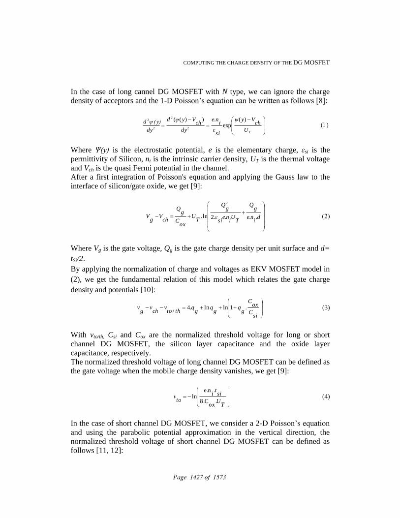
COMPUTING THE CHARGE DENSITY OF THE DG MOSFET
In the case of long cannel DG MOSFET with N type, we can ignore the charge
density of acceptors and the 1-D Poisson’s equation can be written as follows [8]:
TU
chVyψ
siε
ie.n
dy
chVyψd
dy
ψ(y)d )(exp
))((
2
2
2
2
Where Ψ(y) is the electrostatic potential, e is the elementary charge, εsi is the
permittivity of Silicon, ni is the intrinsic carrier density, UT is the thermal voltage
and Vch is the quasi Fermi potential in the channel.
After a first integration of Poisson's equation and applying the Gauss law to the
interface of silicon/gate oxide, we get [9]:
d
ine
gQ
TU
ine
siε
gQ
TU
oxC
gQ
chV
gV ....2ln.
2
Where Vg is the gate voltage, Qg is the gate charge density per unit surface and d=
tSi/2.
By applying the normalization of charge and voltages as EKV MOSFET model in
(2), we get the fundamental relation of this model which relates the gate charge
density and potentials [10]:
siC
oxC
gq
gq
gq
thtov
chv
gv .1lnln.4
/ (3)
With vto/th, Csi and Cox are the normalized threshold voltage for long or short
channel DG MOSFET, the silicon layer capacitance and the oxide layer
capacitance, respectively.
The normalized threshold voltage of long channel DG MOSFET can be defined as
the gate voltage when the mobile charge density vanishes, we get [9]:
TU
sit
toν
.ox
8.C
.i
e.nln (4)
In the case of short channel DG MOSFET, we consider a 2-D Poisson’s equation
and using the parabolic potential approximation in the vertical direction, the
normalized threshold voltage of short channel DG MOSFET can be defined as
follows [11, 12]:
Page 1427 of 1573

COMPUTING THE CHARGE DENSITY OF THE DG MOSFET
l
L
l
L
l
L
l
L
dsν
fφ
biν
toν
thν
sinh
.2sinh
.21
sinh
.2sinh
..2
(5)
Where l is a length that can be defined as follows:
oxt
siε
sit
oxε
oxε
oxt
sit
siε
l..4
.1
.2
..
With vbi and фf are the built in potential between the potential of the source (drain)–substrate junction and the Fermi potential. To define the normalized gate charge density, the relationship between charges
and voltages ((3)) need to be numerically solved for both case long and short
channel DG MOSFET (using the vto in the case of long channel device and vth in
the case of short channel device on the expression (3)).
Considering the drift diffusion transport model, the drain current is obtained by
integrating the mobile charge density in the "x" direction of the channel (from
source to drain) [13]:
dV
sV
chdV
mQ
L
Wμ
dI ..
(6)
Where µ is the constant mobility in channel, W is fixed at 1µm. The mobile charge density per unite surface is defined as follows:
g
Qm
Q .2
After integrating the equation (6) from the source to the drain and achieving the normalization of variables, we get:
mdq
msqsi
C
oxC
mq
oxC
siC
mq
mqi
.2.1ln..2.22
(7)
Finally, the drain current is obtained as follows:
L
W
TU
oxCμi
dsI ....4. 2 (8)
Page 1428 of 1573

COMPUTING THE CHARGE DENSITY OF THE DG MOSFET
3. Numerical procedure
From the expression (3), which relates the potentials and the gate charge density,
we can see that the model is built on an implicit solution. This implicit formulation
is not suitable for circuit simulation and circuit design application.
To compute the mobile charge density without any iterative calculation, the
explicit solution of the gate charge density in a weak and a strong inversion must
be defined.
Before the determination of the gate charge density in a weak and a strong
inversion, we rewrite the fundamental equation of the model (3) with
v (to
vch
vg
v ), si
C
oxC
α and q (g
q ), we obtain [14]:
qαqqv .1.ln.4
(9)
3. 1 Explicit solution of the gate charge density in strong inversion
In this case, the inversion charge density is important (q >> 1). By applying the
Taylor series development to the first order of the term qαq .1.ln around t
qq ,
we get the following expression:
tqα
tqα
tqq
tqq
tqα
tqqv
.1
..21.2.1ln.4
(10)
This expression (10) can be rewrite as the following polynomial equation:
0)]([..4.4 2 vab
tqqvba
tqq
(11)
Where: t
qα
tqα
a.1
)..21.(2
and )).1(ln(
tqα
tqb
Therefore, the expression (11) represents a second order polynomial, where its
solution is given by:
tqa
tq
bav
tq
bavq .2
2
44.2/1
0
(12)
By substituting q0 in qαq .1.ln of the expression (9), we get the explicit solution
of the gate charge density in the strong inversion:
0.1.
0ln.4/1 qαqvqS
(13)
Page 1429 of 1573

COMPUTING THE CHARGE DENSITY OF THE DG MOSFET
3.2 Explicit solution of the gate charge density in weak inversion
In this case, the inversion charge density is very small (q<<1), which implies that
the logarithmic term is dominant compared with the first term in the expression
(9). The expression (9) can be rewritten as follows [14]:
)(ln/1ln qFqv W
(14)
Where))lnΔexp(..1ln()lnΔexp(.4
1)(ln
qqαqt
q
qW
F
and t
qqq lnlnlnΔ
By applying the Taylor series development applied to the first order of the term
)(lnqW
F around 0lnΔ q , we can get:
q
tqα
tq
tqα
tqα
tq
tqα
tq
qW
F lnΔ)).1ln(.4).(.1(
).41(41
).1ln(.4
1)(ln (15)
The substituting of the solution of (15) into (14) let us obtain a new polynomial
expression which is defined as:
0ln.
ln.ln
12ln.1
b
tqv
vaqb
vt
b (16)
Where ).1ln(.4t
qαt
qa and αα
tq
tqαa
b
)1.(4
).1(
The solution of the expression (16) is given by:
ab
tqbv
tqbvq 42)]ln([)ln(.2/1
0ln (17)
After substituting the solution of (17) into the expression qαqqv .1.ln.4 0 ,
the explicit solution of the gate charge density in weak inversion can be written as:
)0
4exp(.4/12/1
)0
4exp(
qvα
qvqW
(18)
After defining the gate charge density in a weak and a strong inversion, a
linearization of the gate charge density and its approximate value is done in both
cases, from that we can get:
).1(10
δKδqq (19)
Page 1430 of 1573

COMPUTING THE CHARGE DENSITY OF THE DG MOSFET
0 0.2 0.4 0.6 0.8 1 1.2 1.40
0.2
0.4
0.6
0.8
1
1.2x 10
-3
Gate voltage [V]
Dra
in c
urr
ent [A
]
Vds=1 V
Vds=0.5 V
Vds=0.2 V
L=1 µmtsi=25 nmtox=2 nm
0 0.2 0.4 0.6 0.8 1 1.2 1.40
0.2
0.4
0.6
0.8
1
1.2x 10
-3
Drain voltage [V]
Dra
in c
urr
ent [A
]
L=1 µmtsi=25 nmtox=2 nm
Vgs=1.4 VVgs=1.4 VVgs=1.4 VVgs=1.4 V
Vgs=1.2 V
Vgs=0.6 V
Where
0
0
0
000
1
214
)1(ln4
qα
qαq
qαqqvδ
With k is a parameter which depends on the operating region of the DG MOSFET
transistor (fixed after numerical experiments, kw = 0.35 for the weak inversion and
ks = 0.13 for the strong inversion).
In order to separate the operating regions of the DG MOSFET transistor (weak and
strong inversion), we use the voltage transition which is defined as following:
)1(ln4
tqα
tq
tq
tv (20)
Where t
q is the transition charge which is fixed after some numerical experiments
at 0.3 for long channel case and 0.12 for short channel device.
4. Results and discussions
(a) (b)
Figure.2. Drain current characteristics: (a) Output characteristic, (b) Transfer characteristic versus drain
and gate voltage
Lines: Our solution; Symbols: Silvaco Atlas-TCAD.
As shown in Fig. 2, for different values of the drain voltage (0.2, 0.5 and 1V) and
the gate voltage (0.6, 1.2 and 1.4V), the drain current for a long channel model of
symmetrical DG MOSFET offer a good agreement with 2-D numerical simulation
using SILVACO Atlas TCAD software.
Page 1431 of 1573

COMPUTING THE CHARGE DENSITY OF THE DG MOSFET
0 0.2 0.4 0.6 0.8 1 1.2 1.40
5
10
15
The n
orm
aliz
ed m
obile
charg
e d
ensity
Gate voltage [V]
Our calculation method
The Newton-Raphson method
Vds=1 V
L=1 µmtox=1.5 nmtsi=30 nm
Figure.3. Comparing the computing mobile charge
density of our method calculation with the
Newton- Raphson one.
Figure.4.The computing mobile charge density
versus the gate voltage with
different silicon thickness.
As shown in Fig. 3, that we also compare our method with the iterative
calculation using the Newton-Raphson method. We can observe a good
agreement with this method, on one hand. But the main advantage of our method
lies in the substantial gain in computation time.
As shown in Fig. 4, for different values of the silicon thickness (10, 20 and
30nm), the mobile charge density have a good behavior from a weak to a strong
inversion and well dependence on the silicon layer thickness.
(a) (b)
Figure.5.The Transfer characteristic: (a) For different channel length, (b) For different oxide thickness.
Lines: Our solution; Symbols: Silvaco Atlas-TCAD.
0 0.2 0.4 0.6 0.8 1 1.2 1.40
0.2
0.4
0.6
0.8
1
1.2
1.4
1.6
1.8
2x 10
-3
Gate voltage [V]
Dra
in c
urr
ent [A
] L=1 µm
L=0.6 µm
tsi=25 nmtox=2 nm
Vds=1 V
0 0.2 0.4 0.6 0.8 1 1.2 1.40
0.5
1
1.5x 10
-3
Gate voltage [V]
Dra
in c
urr
ent [A
] tox=1.5 nm
tox=2 nm
Vds=1 V
tsi=25 nmL=1 µm
0 0.2 0.4 0.6 0.8 1 1.2 1.40
5
10
15
The n
orm
aliz
ed m
obile
charg
e d
ensity
Gate voltage [V]
tsi=10 nm
tsi=20 nm
tsi=30 nmL=1 µmtox=1.5 nm
Vds=1 V
Page 1432 of 1573

COMPUTING THE CHARGE DENSITY OF THE DG MOSFET
0 0.2 0.4 0.6 0.8 1 1.2 1.40
0.002
0.004
0.006
0.008
0.01
0.012
Gate voltage [V]
Dra
in c
urr
en
t [A
]
L=1.2 µm
L=100 nm
tsi=25 nmtox=2 nm
Vds=1 V
This figure show the influence of the channel length (0.6, 1µm) and the oxide
thickness (1.5, 2 nm) on the drain current versus the gate voltage. We can see that
the decreases in the channel length and the oxide thickness are accompanied with
a significant increase in the drain current.
Figure.6. Validation of the computed drain current as a function the gate voltage for long and
Short channel DG MOSFET
. Lines: Our solution; Symbols: Silvaco Atlas-TCAD.
In this last figure, we show the validation of the calculated drain current for long
(1.2 µm) and short (100 nm) channel DG MOSFET with Silvaco software. Good
agreement is also observed.
5. Conclusion
An efficient numerical method to calculate the gate/mobile charge density and the
drain current for long and short channel DG MOSFET model has been presented.
The model describes the static behavior of the long and short channel transistor
and it is continue from weak to strong inversion. The proposed method can
calculate the mobile charge density without any iterative procedure, with a faster
computation time (time simulation) and it is valid for both cases of the device
model.
Our results show a good agreement compared with the iterative calculation using
the Newton-Raphson method, especially, with 2-D numerical simulations from
ATLAS-TCAD (commercial software).
It is showed that the decreases of the technological parameters (channel length and
the oxide thickness) are accompanied, in the case of DG MOSFET structure with
the increase in the drain current.
The normalized equations of the presented model associated with the proposed
method, which compute the mobile charge density for long and short channel
Page 1433 of 1573

COMPUTING THE CHARGE DENSITY OF THE DG MOSFET
transistor give the opportunity for them to be used in circuit simulation. Mixed
mode simulation can be considered.
References:
[1] L. Y. LI, H. M. CHOU, A comparative study of electrical characteristic on
sub-10-nm double-Gate MOSFETs, IEEE Trans. Nanotechnology, vol. 4,
no. 5, pp. 645–647, Sep. 2005.
[2] F. BALESTRA, S. CRISTOLOVEANU, Double-gate silicon-on-insulator
transistor with volume inversion: A new device with greatly enhanced
performance, IEEE Electron Device, vol. EDL-8, no. 9, pp. 410–412,
1987.
[3] F. J. GARCIA-SÁNCHEZ, A. ORTIZ-CONDE, Subthreshold behavior of
undoped DG MOSFETs, IEEE Conf. Electron Devices, Solid-State
Circuits, Dec. 19–21, 2005, pp. 75–80.
[4] N. ARORA, MOSFET Modeling for VLSl Circuit Simulation: Theory and
Practice, World Scientific, 1993, ISBN-13 978-981-256-862-5.
[5] G. BACCARANI, S. REGGIANI, A Compact Double-Gate MOSFET Model
Comprising Quantum-Mechanical and Non-Static Effects, IEEE
Transactions on Electron Devices,vol. 6, no. 8, pp. 1656-1666, 1999.
[6] H. LU, Y. TAUR, An Analytic Potential Model for Symmetric and
Asymmetric DG MOSFETs, IEEE Electron Devices Letters, IEEE Trans.
Electron devices, vol. 53, no. 5, 2006.
[7] L. GE, J. G. FOSSUM, Analytical modeling of quantization and volume
inversion in thin Si-film DG MOSFETs, IEEE Trans. Electron Devices,
vol. 49, no.2, Fev 2006.
[8] Y. TAUR, X. LIANG, A continuous, analytic drain-current model for DG
MOSFETs, IEEE Electron device Letters, vol. 25, no. 2, pp. 107-109,
2004.
[9] J.M. SALLESE, F. KRUMMENACHER, A design oriented charge-based
current model for symmetric DG MOSFET and its correlation with the
EKV formalism, Solid-State Electronics, vol. 49, no. 3, pp. 485-489, 2005.
[10] C. ENZ, F. KRUMMENACHER, An analytical MOS Transistor Model Valid
in All Regions of Operation Dedicated to low voltage and low current
applications, Analog and integrated Circuits and Signal Processing, Vol.
8, pp. 83-114,1995.
[11] Z.H.LIU, Threshold Voltage Model for Deep-Submicrometer MOSFET’s,
IEEE Trans. Electron Devices, vol. 40, no. 1, pp. 86-95, 1993.
Page 1434 of 1573

COMPUTING THE CHARGE DENSITY OF THE DG MOSFET
[12] B.DIAGNE, Explicit compact model for symmetric double-gate MOSFETs
including solutions for small-geometry effects, Solid-State Electronics,
vol.52.pp. 99–106, 2008.
[13] A. AMARA, Planar Double-Gate Transistor from technology to circuit,
Springer, 2009, ISBN-978-1-4020-9341-8.
[14] F. PREÉGALDINY F. KRUMMENACHER, An explicit quasi-static charge-
based compact model for symmetric DG MOSFET, NSTI-Nanotech 2006,
WCM, 2006;3:686, ISB-0-9767985-8-1.
Page 1435 of 1573

Proceedings of the 12th International Conference on Computational and Mathematical Methods in Science and Engineering, CMMSE2012 La Manga, Spain, July, 2-5, 2012
Effective rate constants for nanostructured heterogeneous catalysts
N. Lund1, X. Y. Zhang
2, N. Gaston
1,2 and Shaun C.
Hendy1,2
1MacDiarmid Institute for Advanced Materials and Nanotechnology, School of Chemical and Physical Sciences, Victoria University of
Wellington, Wellington 6140, New Zealand
2Industrial Research Ltd, Lower Hutt 5010, New ZealandFirst
email: [email protected]
Abstract
When reactants are plentiful, the activity by mass of a nanoparticulate catalyst will increase as its surface area increases. Under diffusion-limited conditions, however, the reactant must diffuse to active sites on the catalyst, so a high surface area and a high density of active sites may bring diminishing returns if reactant is consumed faster than it arrives. Here we apply a mathematical homogenisation approach to derive simple expressions for the effective reactivity of a nanostructured catalyst under diffusion limited conditions that relate the intrinsic rate constants of the surface sites presented by the catalyst to an effective rate constant. We show that distinct limiting cases emerge depending on the degree of overlap of the reactant depletion zone about each site. Key words: catalysis, homogenization theory
1. Introduction
There is currently a high level of interest in the use of nanostructured materials for catalysis [1,2]. With precious metal catalysts such as platinum, palladium and gold in high demand, the use of these materials in nanoparticle form can also substantially reduce the cost of the catalyst through the exposure of more surface area for the same volume of material [3]. When reactants are plentiful, the activity by mass of a nanostructured catalyst will increase with its surface area, assuming
Page 1436 of 1573

EFFECTIVE RATE CONSTANTS FOR NANOSTRUCTURED CATALYSTS
that its shape is held constant. However, under diffusion-limited conditions, high surface area and a high density of active sites may bring diminishing returns as active sites consume reactant faster than it arrives. Here we apply a mathematical homogenisation approach [4] to derive simple expressions for the effective reactivity of a nanostructured catalyst under diffusion limited conditions. These expressions relate the intrinsic rate constants of the surfaces presented by the catalyst to an effective rate constant. When highly active catalytic sites, such as step edges or other defects are present, we show that distinct limiting cases emerge depending on the degree of overlap of the reactant depletion zone about each site. In gases, the size of this depletion zone is approximately the mean free path of the gas molecules, so the effective reactivity will depend on the structure of the catalyst on that scale.
2. Theory
We consider a diffusion-limited heterogeneous catalysis reaction scheme. For instance, if we consider the oxidation of a gas Ag on a platinum-group metal catalyst, under conditions where O2 is abundant and readily participates in the reaction while the gas Ag is dilute, then we can restrict ourselves to the following reaction scheme
(1)
(2)
(3)
where Si is a vacant reactive surface site with associated rate constants k1, k2 and k3 respectively. To simplify the analysis, we will assume that step (3), the desorption of the product Bg, occurs much more rapidly than the reaction step (k2
≪ k3) , ignore the desorption of the reactant (i.e. the reverse of step (1)) and assume that step (1), absorption, is the rate limiting reaction step at the surface.
To proceed further, we assume that the diffusion of the gas towards the catalyst is described by a Fickian diffusion equation and that the gas concentration has reached a steady state so that the gas density satisfies
. (5)
Balancing the flux of gas Ag into the site i with the rate of absorption of the gas by mass, we obtain a steady state boundary condition for the gas density near the site:
(6)
Page 1437 of 1573

EFFECTIVE RATE CONSTANTS FOR NANOSTRUCTURED CATALYSTS
where is a length that is approximately the ratio of the mean free path of the
gas Ag to the rate constant k1: .
We are interested in the situation where varies over the surface of the catalyst due to the spatial distribution of active sites with differing values of k1 [5]. In an experiment, one would typically measure a single value keff that represents an effective rate for the whole catalyst. Given the distribution and values of the microscopic parameter k1, it is possible to calculate the macroscopic parameter keff in several limiting cases [6]. In particular, if L is the length scale that describes the distribution of active sites (i.e. if L is the period of a spatially periodic function k1
on the surface of the catalyst) and if , then it can be shown from equations
(5) and (6) that where the angle brackets denote a spatial average.
However, if then .
To interpret these results, it is convenient to assume that there are just two types
of rate constant present on the catalyst surface, say with spacing
L. In the first case above, the active sites are narrowly spaced with respect to
leading to where is the area fraction occupied by the
step sites on the catalyst surface. Thus, in this case, the effective activity of the catalyst is dominated by the activity of the highest activity sites. In contrast, when
the active sites are widely spaced with respect to , we find that
. Thus in the second case, the effective activity of the
catalyst is dominated by the activity of the lowest activity sites.
The two key length scales in this argument are thus the length scale on which the
active sites are distributed, L, and the mean free path of the gas molecules. The mean free path is proportional to the diffusion coefficient of the gas, and so under steady state conditions, it will also be proportional to the size of the region over which the gas Ag is depleted about the active sites. Hence, we can conclude that under diffusion-limited conditions, the effective reactivity of a catalyst will depend on the structure of the catalyst on the scale of the mean free path of the gaseous reactants, which in air, under standard conditions is ~ 100 nm.
References:
[1] H. ZHANG, T. WATANABE, M. OKUMURA, M. HARUTA AND N. TOSHIMA “CATALYTICALLY HIGHLY ACTIVE TOP GOLD ATOM ON
PALLADIUM NANOCLUSTER” NATURE MAT., AVAILABLE ONLINE
DOI:10.1038/NMAT3143, 2011. [2] I. X. GREEN, W. TANG, M. NEUROCK AND J. T. YATES JR, “SPECTROSCOPIC OBSERVATION OF DUAL CATALYTIC SITES DURING
Page 1438 of 1573

EFFECTIVE RATE CONSTANTS FOR NANOSTRUCTURED CATALYSTS
OXIDATION OF CO ON A AU/TIO2 CATALYST” SCIENCE, VOL. 333, PP736-739, AUGUST 2011. [3] V. ZIELASEK, B. JÜRGENS, C. SCHULZ, J. BIENER, M. M. BIENER, A. V. HAMZA AND M. BÄUMER, “GOLD CATALYSTS: NANOPOROUS GOLD
FOAMS” ANGEWANDTE CHEMIE INTERNATIONAL EDITION VOL. 45, PP. 8241–8244, DECEMBER 2006. [4] A. BENSOUSSAN, J. L. LIONS, AND G. PAPANICOLAOU, ASYMPTOTIC
ANALYSIS FOR PERIODIC STRUCTURE, NORTH-HOLLAND, 1978. [5] T. ZAMBELLI, J. WINTTERLIN, J. TROST AND G. ERTL
“IDENTIFICATION OF THE "ACTIVE SITES" OF A SURFACE-CATALYZED
REACTION” SCIENCE, VOL. 273, PP.1688-1690, 1996. [6] S. C. HENDY AND N. J. LUND “EFFECTIVE SLIP BOUNDARY
CONDITIONS FOR FLOWS OVER NANOSCALE CHEMICAL HETEROGENEITIES”, PHYSICAL REVIEW E, VOL. 76, 066313, 2007.
Page 1439 of 1573

Proceedings of the 12th International Conference on Computational and Mathematical Methods in Science and Engineering, CMMSE2012 La Manga, Spain, July, 2-5, 2012
A Fast Recursive Blocked Algorithm for
Dense Matrix Inversion
Ryma Mahfoudhi and Zaher Mahjoub
Department of Computer Science , Faculty of Sciences of Tunis, University of Tunis El Manar, Tunis, Tunisia
emails: [email protected], [email protected]
Abstract
There are several approaches for computing the inverse of a dense square matrix, say A, namely Gaussian elimination, block wise inversion, and LU factorization (LUF). This latter is used in mathematical software libraries such as LAPACK xGETRI and MATLAB inv. The xGETRI method consists, once the two factors L and U are known (where A=LU), in inverting U then solving the triangular matrix system XL = U−1 (i.e. LTXT = (U−1)T, thus X = A−1). Equivalently, one could first invert L, then solve the matrix system UX = L−1 for X. Alternatively, one could invert both L and U, then compute the product X = U−1L−1. Each of these procedures involves at least one triangular matrix inversion (TMI). Thus, we wish the TMI ‘kernel’ to be optimized. On the other hand, the Strassen fast matrix inversion algorithm is known as an efficient approach to solve this problem. We propose in this paper a series of different versions for dense matrix inversion based on the ‘Divide and Conquer’ paradigm. A theoretical performance study permits to establish an accurate comparison between the designed algorithms. Our implementation aims to be used in place of the level 3 BLAS Triangular and Dense Matrix Inversions. Efficient performance could be obtained for large matrix sizes. Key words: BLAS, Divide and Conquer, Matrix Inversion, Strassen method.
Page 1440 of 1573

DENSE MATRIX INVERSION
1. Introduction
Dense Matrix Inversion (MI) is a basic kernel in large and intensive scientific applications. Given its cubic complexity, several works addressed the design of efficient algorithms for solving this problem. Starting from the Strassen and the LU factorization method for MI, our main objective is the design of an efficient algorithm for MI that outperforms the BLAS routines. The remainder of the paper is organized as follows. In section 2, we briefly introduce the divide and conquer (D&C) paradigm, then we detail a theoretical study on Strassen and LU methods in section 3. Afterwards, we present several optimised routines required for MI. Finally, we combine the proposed routines in order to develop efficient algorithms that are implemented and compared.
2. Divide and Conquer Paradigm
There are many paradigms in algorithm design. Backtracking, dynamic programming, and the greedy method to name a few. One compelling type of algorithms is called Divide and Conquer (D&C). Algorithms of this type split the original problem to be solved into (equal sized) subproblems. Once the sub-solutions are determined, they are combined to form the solution of the original problem. When the subproblems are of the same type as the original problem, the same recursive process can be carried out until the subproblem size is sufficiently small. This special type of D&C is referred to as D&C recursion. The recursive nature of many D&C algorithms makes it easy to express their time complexity as recurrences. Consider a D&C algorithm working on an input size n. It divides its input into a (called arity) subproblems of size n/b. The combining and conquering takes f(n) time. The base-case corresponds to n = 1 and is solved in constant time. The time complexity of this class of algorithms can be expressed as follows:
T (n ) = O(1) if n = 1 = aT(n/b) + f (n) otherwise.
Let f(n) = O(nδ) (δ ≥ 0), the master theorem for recurrences can in some instances be used to give a tight asymptotic bound for the complexity [1]:
- a<bδ ⇒ ( ) ( )δnOnT =
- a=bδ ⇒ ( ) ( )nnOnT blogδ=
- a>bδ ⇒ ( ) ( )abnOnT log=
Page 1441 of 1573

DENSE MATRIX INVERSION
3. Strassen Algorithm
Let A, B be n*n real matrices. The number of scalar operations required for computing the matrix product C =AB by the standard method is 2n3=O(n3). In his seminal paper [2], Strassen introduced an algorithm for matrix multiplication, based on the D&C paradigm, whose complexity is onlyOn . This algorithm is based on the block decomposition of both matrix A and its inverse. Let n= 2q (q>1), A is partitioned in 4 submatrices of size k=n/2 as follows:
As to its inverse X = A
, we have :
Where
is the Schur complement of A11 in matrix A. The number of matrix multiplications required for computing blocks X11, X12, X21 and X22 in the block form can be decreased below O(n3) through using the seven temporary matrices R1,..R7 according to the following relations [2]: 1: R1 = A
7: X12 = R3R6 2: R2 = A21R1 8: X21 = R6R2 3: R3 = R1A12 9: R7 = R3X21 (3) 4: R4 = A21R3 10: X11 = R1 - R7 5: R5 = R4 - A22 11: X22 = - R6 6: R6 = R
X11 X12
X22
X =
X21
A11
A12
A21
A22
A = (1)
(2)
Page 1442 of 1573

DENSE MATRIX INVERSION
Formulae (3) can be used for a recursive computation of the matrix inverse X. Both relations 1 and 6 in (3) perform inversions of matrices with smaller sizes (k=n/2). By recursively applying the same formulae on these submatrices, we derive the Strassen method for dense matrix inversion (DMI). Recursion can be continued down to matrices of size 1. The original Strassen DMI algorithm is based on the following two principles:
• P1. In steps 1 and 6, recursively compute the inverses of smaller dimension matrices, and recursion is continued down to size 1;
• P2. Use Strassen matrix-matrix multiplication (MM) method to perform all the matrix multiplications (steps 2-4, 7-9).
Let us denote by inv_Strassen(n) the complexity of this algorithm and let MM(k) be the complexity of multiplying two matrices of size k=n/2 by Strassen algorithm. We get :
inv_Strassen(n) = 2 inv_Strassen (n/2) + 6 MM(n/2) + O(n2) = O(nlogn)+ On + O(n2) = On
4. LU Factorization
As previously mentioned, three methods may be used to perform a DMI through LU factorization (LUF). The first one requires two triangular matrix inversions (TMI) and one triangular matrix multiplication (TMM) i.e. an upper by a lower. The two others require one triangular matrix inversion (TMI) and a triangular matrix system solving (TMSS) with matrix right hand side or equivalently left hand side. Therefore we intend to optimize LUF, TMI, TMM and TMSS kernels.
5. Recursive LU Factorisation
To reduce the complexity of LU factorization, blocked algorithms were proposed in 1974. For a given matrix A of size n, the L and U factors verifying A=LU may be computed as follows:
Page 1443 of 1573

DENSE MATRIX INVERSION
ALGORITHM 1
LUF
Input : A, n*n matrix Output : L : lower triangular matrix, U upper triangular matrix Begin If (n=1) Then L=1; U=A Else /* split matrices into four blocks of sizes n/2
(L1, [U1, U2]) = LUF([A 11 A12])
L3= A21 11 ; H = A22 – L3U2 ; (L4, U4) = LU(H)
Endif End
6. Fast TMI Algorithm
We first recall that the well known standard algorithm (SA) for inverting a triangular matrix (an upper or a lower triangular matrix), say A of size n, consists in solving n triangular systems. The complexity of (SA) is as follows [4]:
SA(n)=n3/3+n2/2+n/6 (4) Using the Divide and Conquer paradigm, Heller proposed in 1973 a recursive algorithm [3-5] for TMI. His main idea consists in decomposing matrix A as well as its inverse B (both of size n) into 3 submatrices of size n/2 (see Figure 1, A being assumed lower triangular). The procedure is recursively repeated until reaching submatrices of size 1. We hence deduce:
, , (5)
Therefore, inverting matrix A of size n consists in inverting 2 submatrices of size n/2 followed by two matrix products (triangular by dense) of size n/2. In [3] Nasri proposed a slightly modified version of the above algorithm. Indeed, since B2=–B3A2 and B1= – 1
121
3−− AAA , let Q= 2
13 AA− . From (5), we deduce:
Page 1444 of 1573

DENSE MATRIX INVERSION
AQ A, BA Q (6)
Fig1. Matrix Decomposition in Heller’s algorithm
Hence, instead of two matrix products needed to compute matrix B2, we have to solve 2 triangular matrix systems of size n/2 i.e. A3Q =A2 and (A1)
T(B2)T= –QT.
We precise that both versions are of n3/3+O(n2) complexity [3]. In [4], we compared a recursive algorithm using matrix multiplication, RAMM, with a recursive algorithm using triangular matrix systems solving, RATMSS. We proved that RATSS is faster and achieved the goal of outperforming of the well known BLAS and LAPACK libraries for triangular matrix inversion. We have to notice that our algorithm benefits from Strassen matrix multiplication algorithm, recursive solvers for triangular systems and the use of BLAS routines in the last level. Algorithm RATMSS may be written as follows:
ALGORITHM 2
RATMSS
Begin If (n=1) Then B1 = 1/A1 ; B3 = 1/A3 Q = A2/A3 ; B2 = -Q/A1 Else /* split matrices into four blocks of sizes n/2 B1 = RATMSS (A1) ; B3 = RATMSS (A3) Q = TMSS(A3, A2) ; B2 = TMSS(A1
T,-QT) Endif End
A1
A2 A3
B1
B2 B3
I1
I2 I3
* =
A B I
Page 1445 of 1573

DENSE MATRIX INVERSION
7. Triangular Matrix System Solving (TMSS)
We now discuss the implementation of solvers for triangular matrix systems with matrix right hand side (or equivalently left hand side). This kernel is commonly named trsm in the BLAS convention. In the following, we will consider, without loss of generality, the resolution of a lower triangular matrix system with matrix right hand side (AX=B). Our implementation is based on a block recursive algorithm to reduce the computation to matrix multiplication [5]-[6]. To optimize this algorithm, we will use a fast Algorithm for dense MM i.e. Strassen algorithm [7]-[8]. In [7] the author reported on the development of an efficient and portable implementation of Strassen's MM algorithm. The optimal number of recursive levels depends on the architecture and must be determined experimentally.
ALGORITHM 3
TMSS
Begin If (n=1) then X = B/A Else /* split matrices into four blocks of sizes n/2
X11 = TMSS(A11,B11) ; X12 = TMSS(A11,B12) X21 = TMSS(A22, B21-MM(A21,X11)) X22 = TMSS(A22, B22-MM(A21,X12))
Endif End
8. Triangular Matrix Multiplication (TMM)
Block wise multiplying an upper triangular matrix by a lower one, can be depicted as follows:
Page 1446 of 1573

DENSE MATRIX INVERSION
Then, to compute the dense matrix C=AB of size n, we need: - Two triangular matrix multiplication (an upper one by a lower one) of size n/2 - Two multiplications of a triangular matrix by a dense matrix (TRMM) of size n/2 - Two Dense matrix multiplication (MM) of size n/2
ALGORITHM 4
TMM
Begin If (n=1) Then C = A*B Else /* split matrices into four blocks of sizes n/2 C1 = TMM(A1,B1)+MM(A2,B3) C2 = TRMM(B4, A2) ; C3 = TRMM(A4,B3) C4 = TMM(A4,B4) Endif End
9. Algorithm TRMM
To perform the multiplication of a triangular matrix by a dense one via block decomposition in halves, one requires four recursive calls and two dense matrix-matrix multiplications (MM). Thus the cost is given by: TRMM(n) = 4TRMM(n/2) + 2MM(n/2). In order to optimize this algorithm, we use, as previously mentioned, a fast algorithm for dense MM i.e. Strassen algorithm. Clearly, if any matrix-matrix multiplication algorithm with On complexity is used, then all algorithms presented before with have the same On complexity.
B1
B3 B4
* =
A B C
A2 A1
A4
A1B1 +
A2B3 A2B4
A4B3 A4B4
Page 1447 of 1573

DENSE MATRIX INVERSION
10. Experimental Study
This section is devoted to the experimental results obtained with our implementation of the different versions for DMI as described above. We precise that we determinate the optimal number of recursive levels for each one. We recall that the optimal number of recursive levels depends on the target architecture and must be determined experimentally. The experiments use BLAS library in the last level. We used the g++ compiler under Ubuntu. Table 1 provides a comparison between Strassen algorithm for DMI (STR), the algorithms based on LU factorization i.e. MILU_1 which requires one TMI and one triangular matrix system solving, MILU_2 requires two TMI and one TMM, and the BLAS routine where we used the routine “dgetri” in combination with the factorization routine “dgetrf” to yield matrix inverse.
TABLE I Timing of matrix inversion (second)
Matrix Size
BLAS STR MILU_1 MILU_2 BLAS
STR
BLAS
MILU_1
BLAS
MILU_2
256 0.01 0.02 0.01 0.01 0.53 1 1 512 0.08 0.05 0.05 0.05 1.60 1.63 1.56 1024 0.90 0.41 0.40 0.45 2.20 2.24 1.99 2048 7.16 1.77 1.74 2.03 4.05 4.12 3.53 4096 62.47 15.24 14.31 15.67 4.10 4.37 3.99 8192 562.21 135.40 128.40 140.39 4.15 4.38 4.00
We precise that in the three last columns, we give the execution times ratios e.g. the ratio 1.63 (row 2, column 7) means that MILU_1 is 1.63 faster than BLAS. We remark that the ratios increase the matrix size i.e. Strassen, MILU_1 and MILU_2 are becoming more and more efficient (improvement factor between 15% and 43%) than BLAS.
11. Conclusion We have achieved the goal of outperforming the efficiency of the well known BLAS and LAPACK libraries for dense matrix inversion (DMI). We have notice that our algorithm benefits from Strassen matrix multiplication algorithm, recursive solvers for triangular systems and the use of BLAS routines in the last level. This performance was achieved through efficient reduction to matrix multiplication where we took care of optimizing the recursive decomposition level and also by reusing the numerical computing libraries as much as possible.
Page 1448 of 1573

DENSE MATRIX INVERSION
This leads us to precise some attracting perspectives we intend to study in the future. We may particularly cite the following points.
- Achieve an experimental study on matrix of larger sizes. - Study the stability of these algorithms
References:
[1] A. FKIRI, Ordonnancement de graphes de type ‘Diviser pour régner’ dans des environnements parallèles homogène et hétérogène, Master thesis, Faculty of sciences of Tunis, 2005.
[2] V. STRASSEN, Gaussian elimination is not optimal. Numer. Math., 13, 354–356, 1969.
[3] W. NASRI AND Z. MAHJOUB, Design and implementation of a general parallel divide and Conquer algorithm for triangular matrix inversion, International Journal of Parallel and Distributed Systems and Networks 5(1), 35–42, 2002.
[4] A. QUARTERONI, R. SACCO AND F. SALERI, Méthodes numériques. Algorithmes, analyse et applications, Springer, 2007.
[5] D. HELLER, A survey of parallel algorithms in numerical linear algebra, SIAM Review 20, 740–777, 1978.
[6] R. MAHFOUDHI, A Fast Triangular Matrix Inversion, World Congress on Engineering, London, 2012 .
[7] B. S. ANDERSEN, F. GUSTAVSON, A. KARAIVANOV , J. WASNIEWSKI AND P. Y. YALAMOV , LAWRA - Linear algebra with recursive algorithms, Lecture Notes in Computer Science, 1823/2000, 629-632, 2000.
[8] J. G. DUMAS, C. PERNET, AND J. L. ROCH, Adaptive triangular system solving, Challenges in Symbolic Computation Software, Dagstuhl Seminar, proceedings, 2006.
[9] H. STEVEN, M. ELAINE, R. JEREMY, T. ANNA, AND T. THOMAS, Implementation of Strassen's Algorithm for Matrix Multiplication, ACM/IEEE conference on Supercomputing, proceedings, 1996.
Page 1449 of 1573

Proceedings of the 12th International Conference on Computational and Mathematical Methods in Science and Engineering, CMMSE2012 La Manga, Spain, July, 2-5, 2012
Data Mining with Enhanced Neural Networks
Ana Martinez1, Angel Castellanos
1, Arcadio Sotto
2 and
Luis F. Mingo3
1 Department of Basic Sciences Applied To Forestry Engineering,
Technical University of Madrid (UPM)
2 Department of Chemical and Environmental Technology, ESCET
Universidad Rey Juan Carlos, Madrid
3 Department of Organization and information Structure
Technical University of Madrid (UPM)
emails: [email protected], [email protected],
[email protected], [email protected]
Abstract
This work presents a new method to solve the nowadays
problems about the symbolic knowledge acquisition from the
weights of a Artificial Neural Network (NN). The relationship
among the knowledge stored in the weights, the performance of
the network and the new implemented algorithm to acquire rules
from the weights is explained. The method has been applied in a
system to obtain rules to forecast the volume of wood for a tree.
The method itself gives a model to follow in the knowledge acquisition with enhanced neural networks.
Key words: artificial neural networks, rule extraction, symbolic rules, data mining
1. Introduction
The main problem that Expert Systems (ES) have is produced by the knowledge
acquisition. Besides, being a time-consuming process that make ES very difficult
to build, the quality of the acquired knowledge also depends on many aspects,
Page 1450 of 1573

DATA MINING WITH ENHANCED NEURAL NETWORKS
such as the availability of the domain experts, their expertise, the relationship
between knowledge engineers, and so on.
In order to build ES and to avoid the bottle-neck in the knowledge acquisition
process, automated learning algorithms can be used, these ones will learn from the
examples that are presented. Among the methods that use learning algorithms are
NNs, So NNs are being applied to the ES technology due to the advantages that
the learning algorithms have [1-5]. NN can be useful for the knowledge base
design [6]. However, one of the disadvantages of NN is that the way of
interpreting the concepts learnt is very difficult [7]. This is due because neural
networks have stored the knowledge in the weights linked to the connections, and
therefore, it is to difficult to explain the concepts in the weights from which neural
networks elaborate the correct output. That is the reason Artificial Intelligence is
performing some research about symbolic knowledge acquisition from a neural
network [8]. Obtained rules of the neural network could give to knowledge
engineering new points of view about the domain and new rules to interpret.
This work presents a new method to solve the nowadays problems about the
symbolic knowledge acquisition from the weights of a NN. The former
corresponds to the framework whose idea is to support knowledge acquisition,
where the optimum way of training the network is related with the knowledge that
can be acquired. The relationship among the knowledge stored in the weights, the
performance of the network and the new implemented algorithm to acquire rules
from the weights is explained.
The prediction volume of wood is presented as an application example, where the
whole method is implemented. The presented model has been successfully applied
and it is a tool that can be added to the processing and control methods available.
The method itself gives a model to follow in the knowledge acquisition with NN.
2. Enhanced Neural Networks
In this work we have used Enhanced Neural Networks. The application of
Enhanced Neural Networks (ENN) [9], when dealing with classification problems,
is more powerful than classical Multilayer Perceptron. These enhanced networks
are able to approximate any function f(x) using n-degree polynomial defined by
the weights in the connections. Multilayer Perceptron MLP is based on the fact
that the addition of hidden layers increases the performance of the Perceptron.
Data sets with a no linear separation can be divided by the neural network and a
more complex geometric interpolation can be achieved, provided that the
activation function of the hidden units is not a linear one.
Page 1451 of 1573

DATA MINING WITH ENHANCED NEURAL NETWORKS
The proposed neural networks ENNs are characterized for having different
weights for each different pattern which is introduced to the neural net [10]. Such
mechanism could be thought as a local interpolation in some specific points of the
function f(x) that the pattern set defines instead of the global interpolation that
MLP networks provide. In order to research this property two neural networks
have been used. The assistant network computes the weights of the main network
depending on the input pattern. That is, each pattern produces a set of weights that
is employed in the main network to output the desired response. The main and
assistant networks share the inputs. Mathematically, the previous idea could be
expressed as , being a weight of the main network and the output
of a neuron in the assistant network. Such idea permits to introduce quadratic
terms in the output equations of the network where they were lineal equations
using Backpropagation Neural Networks BPNN with linear activation functions.
As example we considered the equation (1) of a network ENN 1-1 with an
assistant network 1-2.
Fig. 1 ENN 1-1 Lineal
( ) ( ) ( ) (1)
The degree of the equation is 2, is higher than the degree of Perceptron that is 1. In
this way it is possible approximate some non lineal function without lineal
separation, Perceptron cannot do it.
If there are not hidden layers then the degree of the polynomial is two, which is a
quadratic polynomial in the output of the network. The feature of being able to
increase the degree of the polynomial output, adding more hidden layers, makes
this kind of neural network a powerful tool against the MLP neural networks. A
function could be approximated with a certain error, previously fixed, using a
polynomial of n-degree P(x). The achieved error using this polynomial is bound by
a mathematical expression. Then you only have to compute the successive
derivates of f(x) until a certain degree and to generate the polynomial P(x).
Page 1452 of 1573

DATA MINING WITH ENHANCED NEURAL NETWORKS
We have studied the knowledge extraction algorithms applied to a network with n
inputs. Once trained ENN study the weight matrix of the assistant network in
which the weights have been fixed and that provides the weights of the main
network. Knowledge of the ENN is fixed at the matrix of weights of the assistant
network. These weights are the ones we have applied our knowledge extraction
algorithms, which are presented in the following sections. In order to interpret
these weights applied to each ith column of the weights of the assistant network p-
norm . Obtaining a value that associate to the ith input of main network, for
the set of patterns in the application of our algorithms. We use p-norm defined
by ‖ ‖ (∑| | ) ⁄ (2)
3. Material and Methods
We present a method for extracting knowledge from the weights in a new model of
enhanced neural network ENN. Three different stages have been made: first stages
identifying classes of values of the variable to predict, these classes will be
consistent with the rules and allow grouping of similar characteristics and these
characteristics are reflected in the weights of the trained network. Different
classifications carried out by changing parameters such as amplitude of the output
class, division into outputs classes with the same number of patterns, trying to
improve the learning rate for each trained ENN (explained in subsection 3.1)[11].
A second part, when you are training an ENN, it is possible to know the effect
which each one input is having on the network output. This provides feedback as
to which input channels are the most significant. From there, you may decide to
prune the input space by removing the insignificant channels. This will reduce the
size of the network, which in turn reduces the complexity and the training times
and error (explained in subsection 3.2) [12].
One last stage of processing of rules that identified the behavior of the input
variables (antecedent of the rule) in each output classes (consequents of rules).
Finally, when the rules have been established, Therefore there will be achieved a
control system (explained in subsection 3.3). The model presented has been
successfully applied to the prediction volume of wood. ENNs are thus a useful and
very powerful set of tools that can add to the large number of processing and
control methods available.
First Step: the first stage, this method obtains the consequents or the output in a
rule. First of all, it is necessary a normalization of initial set of training patterns,
input and output variables in the interval [-1, 1] using
min
max min
2( )1
( )newdat
x xX
x x
(3)
This standardized set of patterns is ordered from the smallest to the biggest output.
The first option was to divide the whole range [-1,1] in k output intervals with the
same number of patterns in each interval.
Page 1453 of 1573

DATA MINING WITH ENHANCED NEURAL NETWORKS
A second option was proposed, the output is divided into intervals k units wide,
obtaining 2/k training subsets from each output interval I1..I2/k, where Ii=[-1,-l+k)
... I2/k= (1-k,1] and k=1+3,322log10n [13] and n is the number of patterns.Those
intervals will be the consequents of the extracted rules. For each interval Ii, a
training set Si is considered, which output is Ii. For each training set related to the
output Ii, an independent ENNi is trained, as shown in fig. 2.
Finally we developed a new method, named Bisection Method (BM), which was
provided a better error rate in the training of each interval than the other methods
named, and it is discussed below.
1) Bisection Method (BM)
Once the set of patterns has been sorted, the output is divided in two intervals, and
iteratively division is performed. A first division of the values associated to the
output variable, in two intervals: positive output (0, 1] and negative output [-1, 0).
Two independent neural networks are defined in order to be trained. Each one
neural network is trained with n inputs and only one output. Each one of the two
output intervals are divided in two new classes. This division is performed
iteratively, studying the variation of weights. When in a new division the weights
do not change, then go back to the initial division, and finish the division of the
sets of patterns. A division of the set of training patterns is made according to their
outputs, the output range is divided into intervals, for each output interval Ii, a set
of training Si is considered, an independent neural network is trained, as it is
shown in Fig. 2.
The initial pattern set is classified in several subsets and therefore into several
ENNs. When output intervals are fixed, the consequents of the rules have been
fixed by BM.
Obtaining consequent rules or output intervals Ii for a prediction function:
(1) Standardization of all patterns in the interval [-1,1];
(2) Order the set of patterns from low to high output;
(3) Divide the ordered set of patterns S in n subsets S1…Sn, with SiSj= and
Si=S and Ii= [-1, 1] by (BM) in the previous step and so that in each subset Si
all output values have the same sign. Building one ENNi trained with each Si. The
range Ii covered by the output variable in each Si, determines the consequents rules
that are extracted from each ENNi.
NN 1
[-1..-1+k)
X1
Xp
NN 2/k
(1-k..1
X1
Xp
Set of Rules number 1 Set of Rules number k k2/k
Fig. 2 Set of neural networks
Page 1454 of 1573

DATA MINING WITH ENHANCED NEURAL NETWORKS
2) Second Step: Algorithm to Extract Predictive Variables (EM)
Now, the importance of each input variable must be studied for each different
training network ENNi, taking into account the weights in each one, and so we
must repeat the next algorithm for each one ENNi obtained in the first step. In this
process, antecedents should be chosen in order from biggest to smallest absolute
value of the weights of the connections of input variables, in such way, that each
variable antecedent verifies:
(a) Max |wij| (4)
(b) wijujCi> 0 where Ci = -1,1is the kind of inference negative or positive (5)
It can be studied in which range of allowed values of the input variable, along with
the other variables that contribute to the output, is possible to obtain the whole
output range which is being studied. The range of the variables antecedents would
never be the whole interval [-1, 1], due to the sign of the weights will determine if
the variable will be positive or negative according to in Eq.(5).
For determination of the best set of forecasting variables, in each subset of training
Si with output in Ii:
2.1 Analyze the variation of the values of the input variables for each training
subsets Si, in each ENNi calculating the interval (ij-ij, ij+ij) for each variable uj
in Ii.
2.2 For each ENNi built in step-1, extract important input variables or antecedents,
from it:
We have defined two principal sets: CURRENT and UNKNOWN
1. CURRENT = Wi0 (bias)
,varj
i ju s no used
UNKNOWN W
2. Conditions for Stop: if exist values for aj[-1, 1] such
1
,0 ,var .
( )j
i i j j iu used
W W u f z UNKNOWN
and mini i i iz I z I (4)
(f activation function)
Can Stop
Where ai…aj are input values of the variables ui… uj and ui… ujVARS-USED.
If you want get more input variables for the output class Ii (consequent selected)
go to 2.2.3.
3. Choose a new variable ukVARS-NO-USED such |Wik| is maximum value and
where uk such that CiWik0. It gets a new antecedent for the rule.
4. CURRENT = CURRENT + Wik
UNKNOWN = UNKNOWN - |Wik|
VARS-NO-USED = VARS-NO-USED - (uk )
5. Go to step 2.2.2
3) Third Step: Obtaining rules
Page 1455 of 1573

DATA MINING WITH ENHANCED NEURAL NETWORKS
In the previous step, the antecedent of the rules have been obtained, this is the
most influential input variables for each output interval Ii, each trained ENNi.
When the rule R0 has been formulated, the most important condition has been
given for output in a given interval [-b,-c). The rule obtained is that the weights are
provided, as the most important feature of this interval. If ),[ cbui
and ),[ cbui
are the mean and standard deviation of variable ui in the output range [-b,-c). Then
we take as domain and therefore antecedent for this interval, the values that the
variable ui takes on interval ),( ),[),[),[),[ cbucbucbucbuiiii
.
Thus, we obtain as the first major rule or rule over the output interval [-b,-c)
If ai ),( ),[),[),[),[ cbucbucbucbuiiii
output [-b, - c)= Ij.
Or which is the same: If ai ),(,,,, jijijiji uuuu Ij.
Where i is the number of the input variables and j is the number of output
intervals. In this way we are indicating that in the output range Ij, the most
important variable is the i-th input variable and we are giving the values taken by
the i-th input variable for the output set Ij. Finally, the knowledge extraction for
every net ENNj is made, obtaining a rule or a subset of rules for each output
interval. Each rule Rj corresponds to an output interval. Each output interval has
an associated ENNj, the network has been trained and whose weights define the
variables that must be antecedents of each rule. We enunciate more general rules
with one antecedent or finer rules with more than a single antecedent.
Rk: If ui[a, b) ...uj[c, d) Then IK
If the rule is verified for the extreme values of the interval, you will be checking
for the rest of the values within the range of variation of the antecedent.
Fig. 3 Scheme of Symbolic Knowledge Acquisition
4. Data mining using enhanced Neural Networks
We have studied the behavior of the weights of the network, for a first data set
defining a function exactly. It is a collection of values that define a functional
Page 1456 of 1573

DATA MINING WITH ENHANCED NEURAL NETWORKS
relationship (deterministic) 1,.., ny f x x . If the network is trained in which the
input patterns are the independent variables in the functional relationship and the
output pattern of the network is the dependent variable y. The network learns the
relationship among the variables and the values which constitute the dependent
variable are predicted by ENN. We have studied this case, to check the level of
knowledge stored in the weights. The relationship between the independent
variable and the dependent variable is shown in the values of the weights, some
examples are explained below. A table of values for independent variables and the
corresponding values for the dependent variable is performed. With these data the
network is trained. Table 1 Weights functions
Function Bias Weights X Weights Y
yx 3 -0.0002 0.6201 1.7628
yx 5 -0.0001 0.427 2.003
22 yx -0.6239 1.273 1.273
Table 1 shows as the value of the weights preserves the relationship between the
independent variables, the weight of the variable y is three times that of the
variable x in the first case and in the second case is actually five times the weight
of the variable x the weight value of the variable y, in both cases the variable with
the most influential is the variable y, with different degrees in each case. The
importance of the input variables is reflected in the weights. In the third case, not
working with a linear function, but this is a case in which the behavior of the
variables is symmetrical, both variables influence in the same way in the output
value. With different ENNs have been obtained similar weights. This study has
confirmed that the knowledge of the network, once trained, is stored in the
weights.
We have studied the function f(x, y)=x+y2 and we have generated random patterns
for the variables x and y, then we have observed the behaviour of the weights
changes according to the range of input values. So if we work with values obtained
at random in the interval [1,100] for the input variables x and y the weights
obtained have different characteristics that if we work with values for input
variables in the interval [0, 1]. It seems clear that when a variable takes values in it
[0, 1] and is squared, the value of the variable will decrease, as in this way is
described by the values of the weights for the variable y. However, if the variable
takes values greater than 1 then the variable is greater than being squared. Both
features for the same function are reflected in the weights of the trained networks
for different range of the input variable y (see Table 2 and Table 3).
Page 1457 of 1573

DATA MINING WITH ENHANCED NEURAL NETWORKS
Table 2 The weights function f(x , y)=x+y2 over different range.
Domain input variables Weights x Weights y Mean Square Error
[0, 100) 0.0121 1.3807 0.101
[1, 100] 0.0413 1.6128 0.003
[0, 1] 0.6175 0.6431 0.002
Values obtained with Neurosolution [14]
Working with R the results reflect the same trend.
Table 3 The weights function f(x , y)=x+y
2 over different range.
Domain input variables Weights x Weights y Mean Square Error
[1, 2] 9.838 27.027 0.030
[0.5, 1] 2.776 0.274 0.002
Results obtaining with R (is a free software environment for statistical computing)
All results show that the importance of the input variables change when the range
of input variables change. Yet it is confirmed that the proposed method depends
on:
• First step: divide the set of patterns for its outputs and the study of
interrelationships between the input and output variables. Sometimes, the variation
in the range of the output variable causes changes on the importance of input
variables and then it is necessary to divide the range of the output variable in class,
for a separate study of each output class.
• Second step: study the range and weights of the input variables in each range of
the output variable obtained in the previous step.
• Third Step: extract rules using steps one and two.
5. Example of application
Volume parameter is one of the most important parameters in forest research when
dealing with some forest inventories. Usually, some trees are periodically cut in
order to obtain such parameters using cubical proofs for each tree and for a given
environment. This way, a repository is constructed to be able to compute the
volume of wood for a given area or forests and for a given tree species in different
natural environments. The data set file [15] has been used in order to implement
method explained in the section 3. The example of application is a dataset from
eucalyptus obtained from a region in Spain. The main aim is to detect relationships
between all the variables that are in our study, and also this work seeks to estimate
the wood volume. The input variables considered for the network were diameter,
thickness bark (crust); grow of diameter, height and age. The output variable was
the volume of wood.
The Enhanced ENNs were trained, but in any case learning didn’t improve,
initially tested the whole set. The ratio of error should not be acceptable; the
Page 1458 of 1573

DATA MINING WITH ENHANCED NEURAL NETWORKS
knowledge learned by the network is not good, the error is too large. The
evolutions of the values of the weights, in different division intervals for all
patterns, the first division in positives and negatives outputs in, finally four
networks have been trained for 145 patterns. The error is less when the total
pattern set is divided in subsets and one ENN is trained for each subset of pattern.
In this example, finally 4 neural networks were constructed: one for each set of
patterns S1…S4 obtained, which outputs are I1…I4, .One neural network is trained
for each interval. Now, in each one of the sets of patterns obtained, the most
important input variables, in each one of the subsets is sought, using the algorithm
for extraction (EM). Below, in Table 4 is showed the weights of the four trained
networks obtained in the first phase BM.
In the second step, the method named as EM has been implemented. Now when
the set is divided into four subsets and the weights are observed in each obtained
subset or class, it is possible to detect that the most important input variable is
changing in each class, by the weights in each neural network. The crust appears
as the most important variable followed by height in the first class, in the class two
the most important input variable has changed and now the principal variable is
the diameter and in the third class the same importance for diameter and height
and in the fourth class is the diameter the most important variable again. Weights
are studied when they are stable and do not change.
Table 4 The most important input variables: weights hidden layer over each output interval volume
class Age Diameter Height Crust Active performance
1 -0.147 -0.046 0.705 1.279 MSE = 0.060
2 0.036 0.788 0.596 0.586 NMSE = 0.110
3 0.142 0.670 0.669 0.495 MSE = 0.019
4 -0.181 0.840 0.8248 0.57 NMSE= 0.062
Table 5 Values of the variables in each ENNi. Domain antecedents of rules.
Class Volume Diameter/cm Crust Height/m Age
Average 1 43.39 9.55 8.84 11.9 12.9
Desviation 1 20.7 2.06 4.76 2.32 4.54
Average 2 95.13 13.13 17.4 16.41 12.9
Desviation 2 12.55 1.16 5.16 1.62 4.44
Average 3 161.33 15.61 26.087 19.48 1.4
Desviation 3 25.24 1.27 5.66 2.03 3.38
Average 4 476.87 22.89 69.3 25.88 15.43
Desviation 4 226.21 4.19 30.1 4.33 2.53
Table 5 shows the possible domain of antecedents of the rules. In third step the
solution is a set of rules. Using sections 3.2 and 3.3, the following rules have been
Page 1459 of 1573

DATA MINING WITH ENHANCED NEURAL NETWORKS
obtained from the nets. To apply the rules extracted above to the studied case
about volume of wood. The rules show that the network has learned, and then it is
possible get a good set of rules if there was a good learning ratio in the training
network. For each output interval a set of rules is obtained with one or more
variables as antecedents, so the rules are obtained:
4,13.6 9.5,14.2 22,64If crust height volume
12,14.3 12.4,22.5 82,107If diameter height volume
14.3,16.8 20.4,31.7 136,186If diameter height volume
18.2,27 39,99 250,703If diameter height volume
14.3 20.4 136If diameter height volume
14.3 40 136If diameter crust volume
The problem under study is prediction of volume of wood, and the rules obtained
are useful in order to estimate the amount of wood using typical tree variables and
the Knowledge obtained is compared with other methods such as repository and
with the tree volume tables for a given tree species and for prediction methods as
regression. The results are similar in each case.
6. Conclusions
A new method to extract rules from a neural net has been elaborated, in this way;
the rules obtained will allow completing the knowledge that could be extracted
from an expert when building the knowledge base for an ES. In the proposed
method, a model of neural network Enhanced Neural Network has been used. The
implemented method is effective when the importance or characteristics of
forecasting variables could change depending on the range of forecast variable.
The proposed method has been developed in three parts: a study of the weights in
the enhanced neural network by dividing the pattern set into subsets (BM), so you
get two benefits, the ENN detects a possible change in the importance of the input
variables (for each one of the subsets obtained after the division) and an
improvement in learning rate. In the second part by the algorithm (EM) to obtain
the most important input variables for each subset, and finally in the third part
building for each division obtained a rules database. The output of the net has a
lower mean squared error, thus a more accurate set of rules is obtained. We have
compared the results obtained with rules with other methods as tables of scaling
for trees of this species and statistical forecasting models, in both cases, the results
are similar to those obtained by the proposed method. The advantage ENN is each
new data can be updated and improved the database, more easily and can go to
expand the database of rules obtained.
Page 1460 of 1573

DATA MINING WITH ENHANCED NEURAL NETWORKS
References:
[1] J. HEH, J.C. CHEN, Designing a decompositional rule extraction algorithm
for neural networks with bound decomposition tree, Neural Comput. &
Applic. 17(3) (2008) 297-309.
[2] J.A. MALONE, K.J. MCGARRY, C. BOWERMAN, Rule extraction from
Kohonen neural networks, Neural Comput. & Applic. 15 (2006) 9–17.
[3] R. SETIONO, W. KHENG, J. ZURADA, Extraccion of rules from neural
networks for nonlinear regression, IEEE Trans. Neural Network vol. 13(3)
(2002) 564–577.
[4] R. ANDREWS, S. GEVA, Rule extraction from local cluster neural nets.
Neural Comput.(2002) 47, 1–20
[5] Z. BOGER, H. GUTERMAN, Knowledge extraction from artificial neural
networks models. Proc. IEEE Int. Conf. Systems, Man and Cybernetics
(1997) 3030–3035.
[6] S.M. KAMRUZZAMAN , A. M. JEHAD SARKAR, A new Data Mining scheme
using neural networks, Sensors 2011, 11, 4622-4647;
doi:10.3390/s110504622
[7] E. KOLMAN, M. MARGALIOT, Are artificial neural networks white boxes?
IEEE Trans. Neural Net. 16 (2005) 844–852
[8] H. TSUKIMOTO, Extracting rules from trained neural networks, IEEE Trans.
Neural Network 11 (2000) 377–389
[9] L.F. MINGO, A. MARTINEZ, V. GIMENEZ, J. CASTELLANOS, Parametric
Bivariate surfaces with Neural Networks, Machine Graphics and Vision,
vol. 9, no. 2. (2000) pp. 41-46.
[10] L.F. MINGO, S. ABLAMEYKO, L. ASLANYAN, J. CASTELLANOS, Enhanced
Neural Networks with Time-Delay in Trade Sector, Digital Information
Processing and Control in Extreme Situations. DIPCES 2002, Pp.:202-
208.
[11] A. CASTELLANOS, J. CASTELLANOS, D. MANRIQUE, A. MARTINEZ, A new
approach for extracting rules from a trained neural network, Lect. notes
Comput. Sci. 1323 (1997) 297-302.
[12] A. MARTINEZ, A. CASTELLANOS, C. HERNANDEZ, F. MINGO, Study of
weight importance in NN, Lect. notes Comput. Sci. 1611 (2004) 101-110.
[13] H. A. STURGES, The choice of a class interval, Journal of the American
Statistical Association, Vol. 21, No. 153 (1926), pp. 65-66. DOI:
10.2307/2965501.
[14] Neurodimension.Inc. Software: Neurosolution V. 5.
http://www.neurosolutions.com Accessed 20 June 2010.
[15] Dataset.http://acer.forestales.upm.es/basicas/udmatematicas/matematicas1/datos/Eucaliptos.pdf
(2011). Accessed 10 march 2012.
Page 1461 of 1573
Proceedings of the 12th International Conference on Computational and Mathematical Methods in Science and Engineering, CMMSE2012 La Manga, Spain, July, 2-5, 2012
Numerical methods for unsteady blood flow interaction with nonlinear viscoelastic arterial vessel wall
Felix Mihai2, Inja Youn1 and Padmanabhan Seshaiyer2,* 1 Department of Mathematical Sciences, George Mason University
2 Department of Computer Science, George Mason University
emails: [email protected], [email protected], [email protected]
Abstract
Mathematical modelling and simulation of fluid-structure interaction of multi-physics applications often requires the numerical solution to complex coupled partial differential equations. This may be accomplished by efficient domain decomposition techniques which involve partitioning the global computational domain (on which the coupled process evolves) into several sub-domains on each of which local problems are solved. The solution to the global problem is then constructed by suitably piecing together solutions obtained locally from independently modelled sub-domains. In this paper we develop a multilevel domain decomposition approach for coupled fluid-structure interaction problems applied to a multi-physics application involving atherosclerotic arteries. The model will incorporate both geometric nonlinearity and material nonlinearity as well as visco-elasticity for the arterial wall and a non-axisymmetric plaque that interacts with unsteady blood flow. In particular, these models indicate the generation of recirculation zones at various locations near the plaque which could potentially enhance the risk of the formation of a clot. The importance of the nonlinear and viscoelastic material models that contribute to this is studied in this work. Key words: fluid-structure; multi-physics; viscoelasticity MSC2000: AMS Codes (optional)
* Corresponding Author: Padmanabhan Seshaiyer, Professor, Mathematical Sciences, George Mason University, Fairfax, VA 22030.
Page 1462 of 1573

NUMERICAL METHODS FOR FSI
1. Introduction Fluid-structure interaction of multi-physics applications often involve complex dynamic interactions of multiple physical processes and functionally distinct components. In these applications, the challenge is to understand and develop algorithms that allow the structural deformation and the flow field to interact in a highly non-linear fashion. Not only is the non-linearity in the geometry challenging but in many of these applications the material is non-linear and visco-elastic as well that makes the problem even more complex. Direct numerical solution of the highly non-linear equations governing even the most simplified two-dimensional models of such fluid-structure interaction, requires that both the flow field and the domain shape be determined as part of the solution, since neither is known a priori. Cardiovascular atherosclerotic arteries that often consist of diseased plaques are known to be the leading cause of health risks and mortality. More specifically, narrowing of an artery that can result from a plaque deposit causes severe reduction of the blood flow. Modeling such diseased arteries requires modeling the unsteady blood flow interacting with the compliant arterial vessel wall as well as a plaque in an efficient way. It is well known that the presence of a plaque can significantly alter the characteristics of the blood flow in arteries which can then lead to the development of cardiovascular atherosclerotic disease. In current clinical practice, the degree of the luminal narrowing determines the need to surgically remove an existing plaque [1]. The Doppler ultrasound technique that is currently employed uses the maximum peak systolic and diastolic blood flow velocities as well as the spectral composition of these velocities. Although this technique is in universal clinical use, there have been problems in the use of this technique. Moreover, due to the nature of the associated strong coupling of the plaque with the blood flow and arterial wall, there is a great need to develop coupled models to understand the displacement of the plaque and its interaction with the flow. These often results in recirculation zones around the plaque that lead to the formation of a thrombus, that eventually leads to a heart attack or a stroke. To estimate the stress levels on the plaque surface, fluid structure interaction analysis has emerged as an efficient computational tool that has combined computational fluid dynamics for the blood with structural mechanics of the surrounding elements such as the arterial wall and the plaque [2, 3]. In these papers, the authors conducted a finite element analysis to examine the fluid structure interaction of pulsatile and unsteady flow through a compliant stenotic artery respectively. They both observed complex flow patterns and high shear stress at the throat of the plaque and their results indicated critical plaque stress/strain conditions are influenced by a variety of biomechanical factors.
Page 1463 of 1573

NUMERICAL METHODS FOR FSI
Most of the prior simulations have used a geometrically linear material approximation. There is a lot of evidence and experimental results that suggest that soft tissues undergo large deformations (which cannot be modeled via an infinitesimal deformation) that make them geometric nonlinear structures. Moreover highly nonlinear stress-strain relations, strong anisotropic mechanical properties and significant viscoelastic features [4] make the modeling challenging which is the focus of this work.
2. Model and Governing Equations Consider the multi-physics interaction of a nonlinear visco-elastic structural domain interacting with an unsteady fluid medium. For simplicity of presentation, we consider the following computational model that involves multiple non-linear structural elements (arterial vessel walls and the plaque deposit) that interact with the unsteady blood flow. The computational domain is illustrated in Figure 1.
Figure 1. Computational Domain for the multi-physics problem
Let the computational domain 2ℜ⊂Ω be an open set with global boundary Γ . Let Ω be decomposed into the four disjoint open sets, a fluid subdomain fΩ and three
solid subdomains isΩ , i =1, 2, 3 with respective boundaries fΓ and sΓ . Let j
IΓ , j= 1,2,3, 4 be the interface between the solid and fluid domains. The structural domain consists of two symmetric arterial vessel walls denoted by 21
, ss ΩΩ and a
domain describing the plaque 3sΩ .
2.1 Modelling the unsteady blood flow We model the fluid domain via the unsteady Navier-Stokes equations for an incompressible, isothermal fluid flow written in non-conservative form as:
fΩ
1sΩ
2sΩ
3sΩ
100 mµ
10 mµ
10 mµ
2IΓ 3
IΓ
1IΓ
4IΓ
1sΩ
Page 1464 of 1573

NUMERICAL METHODS FOR FSI
0
)(
=⋅∇
+⋅∇=∇+∇⋅+∂
∂
ff
ffffff
f
u
Fpuut
u
ρ
τρρ (1)
where fu is the fluid velocity, fρ is the fluid density, p is the pressure and fF is
the body forces. The viscous stress tensor )(2)( ff uDu ητ = where η is the dynamic viscosity and the deformation tensor is given by:
( )
∇+∇=
2)(
Tff
f
uuuD µ (2)
The fluid equations are subject to the boundary conditions:
4,3,2,1,,
,.
4,3,2,1,,
=Γ∈∂∂
=
Γ∈⋅=
=Γ∈=
jxtu
u
xntn
jxuu
jI
sf
Nf
jIwallf
τ (3)
where )(2 fuDpIt +−= is the prescribed tractions on the Neumann part of the boundary with n being the outward unit normal vector to the boundary surface of the fluid. Conditions of displacement compatibility and force equilibrium along the structure-fluid interface are enforced. The weak variational formulation of the fluid problem then becomes solving for the fluid velocity fu and pressure p satisfying:
( )
∫
∫∫∫∫ ∫
Ω
ΩΩΩΩ Ω
=Ω⋅∇
Ω⋅∇⋅−Ω⋅∂∂
−Ω⋅+Ω⋅=Ω∇⋅
f
ffff f
f
ffffffff
duq
duudtu
dtdFd
0
φρφρφφφτ(4)
2.2 Modeling the Structure equations The structural domains consists of the arterial vessel walls denoted by 21
, ss ΩΩ and
the plaque 3sΩ . They are modelled via the following equation:
sss
s Ftu
+⋅∇=∂∂
τρ2
2
(5)
where su is the structure displacement, sρ is the structure density, sτ is the solid
stress tensor and 2
2
tus
∂∂
is the local acceleration of the structure. This is solved with
the boundary conditions:
Page 1465 of 1573

NUMERICAL METHODS FOR FSI
4,3,2,1,..
.
=Γ∈+−=
Γ∈=
Γ∈=
jxtnn
xtn
xuu
jI
ISss
NSsss
DS
Dss
ττ
τ (6)
Here D
SΓ and NSΓ are the respective parts of the structural boundary where the
Dirichlet and Neumann boundary conditions are prescribed. Also st are the
applied tractions on NSΓ and I
St are the externally applied tractions to the interface
boundaries 4,3,2,1, =Γ jjI . the unit outward normal vector to the boundary
surface of the structure is sn . The stresses are computed using the constitutive relations that will be described next. Equation (6) enforces the equilibrium of the traction between the fluid and the structure on the respective fluid-structure interfaces. In continuum mechanics, there are two types of non-linearity that often arises in various applications. The first type is related to the constitutive law that dictates how the material responds to applied loads. This leads to a nonlinear relation between the stress sτ and the strain ε . In this work, we consider two different constitutive models for the structural domains that include a linear elastic, a hyperelastic model and a visco-elastic model. The second type of nonlinearity arises when the strain ε varies nonlinearly with respect to the displacement. The total strain tensor for a typical geometrically non-linear model is written in terms of the displacement gradients:
( )sTs
Tss uuuu ∇∇+∇+∇=
21
ε (7)
For small deformations, the last term on the right hand side is omitted to obtain a geometrically linear model. In this work we will consider geometrically nonlinear model (7) combined with both linear and nonlinear constitutive laws. The solid stress tensor sτ is given in terms of the second Piola-Kirchoff stress S :
( )( )ss uIS ∇+⋅=τ (8) For the linear material model we employ the following constitute law relating the stress tensor to the strain tensor: ε:0 CSS += (9) where C is the 4th order elasticity tensor and “:” stands for the double-dot tensor product, 0S and 0ε are initial stresses and strains respectively. A hyperelastic material is defined by its strain energy density function sW that is a function of the state of the strain in the body. For isotropic hyperelastic materials, the elastic strain energy can be written in terms of three invariants. Normally, the
Page 1466 of 1573

NUMERICAL METHODS FOR FSI
elastic deformation tensor is used (given by elF ) along with the elastic right
Cauchy-Green deformation tensor given by elTelel FFC = . One can then obtain the
elastic Green-Lagrange strain tensor as ( )ICelel −=21ε where I is the identity
tensor. To describe a compressible model, we also require the elastic volume ratio defined by )det( elel FJ = . For the hyperelastic nonlinear material model, we employ the compressible neo-Hookean model:
( ) ( ) ( )[ ]21 log21
log321
elels JJIW λµµ +−−= ε∂
∂= sW
S (10)
For viscoelasticity we use a linear viscoelastic solid whose total stress tensor is given by ds spI +−=τ . The general linear dependence of the stress deviator on the strain history can be expressed by the integral:
tdt
ttst
dd ′
′∂∂
′−Γ= ∫0
)(2ε
(11)
where the function )(tΓ is called the relaxation shear modulus function that can be found by measuring the stress evolution in time when the material is held at constant strain. The relaxation function is approximated in a Prony series. The weak variational form of the structural equations then becomes: Find the structure displacement su such that:
( )∫∫∫∫ ∫ΓΩΓΩ Ω
Γ⋅⋅−−Ω⋅∂∂
−Γ⋅+Ω⋅=Ω⋅If
Nsf f
dntdtu
dtdFd sfIssssssssssss φτφρφφετ
2
2
(12) 2.3 Modeling the coupled fluid-structure system In order to account for the changing nature of the fluid and solid sub-domains, one must define a dynamic mesh for the space discretization. However, to avoid extreme distortion, we choose to move the mesh independently of the fluid velocity in the interior of the fluid domain. Such a scheme, called arbitrary Lagrangian-Eulerian (ALE) formulation, is commonly applied when studying fluid-structure interaction [5, 6]. This choice allows us to use a Lagrangian framework for modelling the structure and a mixed formulation for modelling the fluid. In particular, we express the time derivatives as functions of Lagrangian reference coordinates, while the derivatives with respect to space are left as
Page 1467 of 1573

NUMERICAL METHODS FOR FSI
functions of the fixed Eulerian coordinates. To do this we define a mesh velocity w that describes the velocity of the mesh nodes as a time derivative of the deformation function. The ALE formulation for the fluid equation then becomes:
( ) Fpuwut
uxdxf
L
ff +∇=∇+
∇−+
∂
∂τρ ..
where L is the Lagrangian coordinate, and x the Eulerian coordinate. 2.4 Finite element discretization Let the domain Ω be partitioned into m non-overlapping sub-domains m
ii
1 =Ω such that the intersection of any two sub-domains is empty, a vertex, or a collection of edges of the respective domains. In the latter case, we denote this interface by ijΓ which consists of individual common edges from the domains iΩ and jΩ . Over each subdomain, a fully coupled system is solved for the solution variables, namely, the velocity, the pressure, the stress vector and the structural displacements. The solution to the associated fluid-structure interaction problem is then achieved via an iterative strategy, where the systems of equations (11)-(12) along with the continuity equation are solved separately and in succession, always using the latest information, until convergence is reached. 3. Numerical Results In this section, we will present the performance of the coupled algorithm applied to the model problem presented. In all our experiments, the blood is modelled to enter the artery from the left side via a Poiseuille parabolic profile whose amplitude is time dependent (in order to simulate a cardiac beat). In particular, we model the mean inlet velocity via:
0016.007.0 24
2max
+−=
tt
tuumean (13)
where maxu = 3.33 cm/sec. The time dependence is taken from [7]. The channel height of the artery as indicated before was chosen to be 100 mµ . The fluid density and the dynamic viscosity were chosen to mimic blood properties to be 3kg/m1050=fρ and secPa004.0=fµ respectively. For modelling the structure, we consider three separate cases. Case I: Materially linear and geometrically linear (MLGL) In this model we consider the arterial wall and the plaque to be modelled as geometrically linear and materially linear. Hence the strain tensor is calculated as
( )Tss uu ∇+∇=
21
ε and the isotropic solid stress tensor is expressed in terms of
Page 1468 of 1573

NUMERICAL METHODS FOR FSI
the second Piola-Kirchoff stress S as in (8) and (9). The values of density, Young’s modulus and Poisson’s ratio of the solid were chosen to be 3/1000 mkgs =ρ , 45.0andPa106 == νE respectively. Case II: Materially linear and geometrically nonlinear (MLGN) In this model, we consider the arterial wall and the plaque to be both modelled as geometrically nonlinear and materially linear. In particular, we let the strain tensor to account for the geometric nonlinearity through the quadratic term in
( )sTs
Tss uuuu ∇∇+∇+∇=
21
ε . The material model is chosen to be the same as in
case I. Case III: Materially nonlinear and geometrically nonlinear (MNGN) In this model, we consider the arterial wall and the plaque to be modelled as geometrically nonlinear as in Case II. However, the material is now considered to be hyperelastic compressible neo-Hookean model. We also choose the arterial wall properties to be different from the properties of the plaque. In particular we choose the following values for the arterial wall properties
Pa1045.3,Pa101.3,kg/m1000 563 ×=×== µλρ s and for the plaque we choose
Pa32
20,Pa102.6,kg/m1000 63 µµλµρ −=×==s
In order to be consistent in the values, we choose the Young's modulus and Poisson ratio values to correspond to the values of the Lame constants:
)21)(1(
,)1(2 νν
νλν
µ−+
=+
=EE
The prescribed inlet velocity profile attains a maximum value at about t=0.215 sec. The velocity and stress distributions at four different times are presented in figure 2 for the MNGN model. The maximum values of the von Mises stress and the velocity values for each of these simulations is illustrated in figure 3 and figure 4. Both the multi-physics simulations as well as the maximum values clearly show the importance of including the nonlinear effects in the material and the geometry. The values clearly indicate that the nonlinearity of the geometry increases the value of the stresses and the maximum velocity. These also create multiple recirculation zones with the model in MNGN creating vortex formation (see figure 2) which could potential lead to very high shear stresses near the throat of the plaque. The later can induce thrombosis which can totally block blood flow to the heart or brain. Detection and quantification of such vortices is very valuable and can serve as the basis for surgical intervention.
Page 1469 of 1573

NUMERICAL METHODS FOR FSI
Figure 2: The surface von Mises Stress along with streamlines of spatial velocity field shown at times t=0.1sec (top-left), t=0.215 sec (top-right), t=0.3 sec (bottom-left) and t=4 sec (bottom-right) for the MNGN model.
Figure 3: Comparison of the maximum Von Mises Stresses for all three models
Page 1470 of 1573

NUMERICAL METHODS FOR FSI
Figure 4: Comparison of the maximum velocity for all three models
4. Conclusion In this paper, we presented the mathematical modeling and simulation of a
fluid-structure interaction algorithm applied to a multiphysics application involving atherosclerotic arteries. The model incorporated both geometric nonlinearity and material nonlinearity for the arterial wall and the plaque that interacted with unsteady blood flow. The results clearly indicate the generation of recirculation zones at various locations near the plaque which could potentially enhance the risk of the formation of a clot. Three separate models were considered in this work and their influence on the behavior of the plaque was studied. The results indicate that a plaque modeled as a materially nonlinear and geometrically nonlinear shows evidence of recirculation that is different from those that are modeled using linear models. Such studies are essential to get a good insight into the risk of rupture of a plaque. In this work, we considered the flow to be Newtonian. In the future study we
plan to consider effects of non-Newtonian rheological properties incorporated along with this materially and geometrically nonlinear model developed and presented in this paper. Moreover, the current study needs to be extended to incorporate the visco-elastic wall. Once we have an effective model, then one must develop effective parameter estimation techniques to quantify the biomechanical factors in the model better.
Page 1471 of 1573

NUMERICAL METHODS FOR FSI
References:
[1] P.M. ROTHWELL ET. AL., Analysis of pooled data from the randomized controlled trials of endarterectomy for symptomatic carotid stenosis, Lancet 361 (2003) 107-116.
[2] M. BATHE AND R. D. KAMM, A fluid-structure interaction finite element analysis of pulsatile blood flow through a compliant stenotic artery, ASME Journal of Biomechanical Engineering, 121 (1999) 361-369.
[3] D. TANG ET. AL., Effect of a lipid pool on stress/strain distributions in stenotic arteries: 3D fluid-structure (FSI) models, Journal of Biomechanical Engineering, 126 (2004) 363-370.
[4] FUNG YC., Biomechanics: Mechanical Properties of Living Tissues, New York, Springer, 1993.
[5] J. DONEA, S. GIULIANI, J.P. HALLEUX, An arbitrary Lagrangian-Eulerian finite element method for transient dynamic fluid-structure interactions, Computer Methods in Applied Mechanics and Engineering, 33 (1982) 689-723.
[6] E.W. SWIM AND P. SESHAIYER, A nonconforming finite element method for fluid-structure interaction problems, Comput. Meth. Appl. Mech. Eng., 195 (2006) 2088-2099.
[7] ZHI-YONG LI, SIMON P.S. HOWARTH, TJUN TANG, JONATHAN H. GILLARD. How Critical Is Fibrous Cap Thickness to Carotid Plaque Stability? A Flow Plaque Interaction Model. Stroke 37 (2006) 1195-1196.
Page 1472 of 1573

Proceedings of the 12th International Conference on Computational and Mathematical Methods in Science and Engineering, CMMSE2012 La Manga, Spain, July, 2-5, 2012
A mathematical model for the Container Stowage and Ship Routing Problem
Ana Moura1, Jorge Oliveira1 and Carina Pimentel1
1 Department of Economics, Management and Industrial Engineering, University of Aveiro
emails: [email protected], [email protected],
Abstract
The main goal of this paper is to present a mathematical model for a fleet of containerships with no pre-defined routes, considering demands and delivery deadlines. The short sea shipping is a very complex problem that belongs to the class of routing problems, more precisely, to the Capacitated Vehicle Routing Problem with deadlines and Loading Constraints. In this problem two major decisions must be made: which ports should be visited by each vessel and the related visit sequence, and where to load the containers in vessels in order to prevent overstowing. A mixed integer programming model for the problem is presented and solved. This mathematical formulation intends to contribute to a better management of small fleets of containerships in order to reduce transportation time and delivering costs. Keywords: Mixed Integer Programming, Container Stowage Problem, Vehicle Routing Problem
1. Introduction
Vessels have always been used as means of transport between European ports and, to this day, short sea shipping is responsible for a significant part of all freight moved within the European Union borders. About 70% of international trade cargo is transported by sea in containers. Shipping in Europe represents 40% of intra-community exchanges, which means that a large part of cargo transportation is done over short distances [1]. Maritime transport has lower freight rates compared with air transportation. Moreover, the number of accidents and pollution levels are lower when compared with other means of transport [2].
Page 1473 of 1573

A MATHEMATICAL MODEL FOR CSSRP
The advantages of short sea shipping are well known and recognized by EU member states: it is environmentally sound; it contributes to road safety; it has low infrastructure costs (the sea itself is the “motorway”); and it can reach most of Europe’s “peripheral” regions. Nonetheless, there are also some downsides, namely: the bureaucracy attached to customs; port services costs and efficiency; travel duration; inflexibility of routes; and dependency on environmental factors. This work intends to contribute to a better management of small fleets of containerships in order to reduce transportation costs. The main goal of this work is to present a mixed integer linear programing (MIP) model for a fleet of containerships with capacity constraints, ports deadlines and no pre-defined routes. The routes are planed depending on: distances, demands and delivery deadlines of each port. Besides, the routes are interconnected with the containers loading distribution in order to prevent overstowing. According to these challenges, two different kinds of optimization problems must be dealt with, in an integrated manner: the Vessels Routing Problem with Time Deadlines and the Container Stowage Problem. We named the integration of these two problems as the Container Stowage and Ship Routing Problem (CSSRP). The CSSRP has received little attention in the literature. All the approaches we were able to find have only considered the ships’ container stowage problem, sometimes with port deliveries considerations, given a predefined port visiting route. Nevertheless, as far as we know there is no work in the literature dealing with the Container Stowage Problem (CSP) and the well-known Vehicle Routing Problem (VRP) with deadlines in an integrated way. The remainder of the paper is structured as follows: section 2 consists of a review of the relevant literature; in section 3 we introduce the CSSRP, where constrains and problem characteristics are explained; in section 4 a mixed integer programming model is presented; section 5 is dedicated to the discussion of some preliminary results, considering some generated problem instances, and to the analysis of the model performance; to conclude, we summarize some global remarks and suggestions for future work in the last section (section 6).
2. Literature Review
The Container Stowage Problem, also known as the Master Bay Problem, is a NP – hard problem [3] and is concerned with the task of determining the arrangement of containers in a containership. The CSP can be explained as an assignment problem where a set of containers with a given port destination, each one with different characteristics, must be assigned to slots in a vessel aiming to minimize the transportation cost. In each port there are several handling operations that may force some containers to be moved and rearranged. These handling operations are due to several reasons: the containers reached their destination port; the vessel stability must be ensured; overstowing situations must be overcome. An overstow occurs when there are containers that must be moved because they block the
Page 1474 of 1573

A MATHEMATICAL MODEL FOR CSSRP
access to other containers that have to be unloaded. In each port, the handling operations have an associated cost that must be minimized. Later on this cost will be detailed. Besides, there are other aspects that may have to be considered too in CSP: (i) the sequence of visiting ports; (ii) the time limit to deliver the containers demanded in each port; (iii) the capacity of vessels; (iv) the stability of the containership (horizontal and cross stability); (v) weight constraints, when containers are stacked above each other and on decks; (vi) accessibility constraints; (vii) mixture constraints, when containers of different sizes are stacked together and (viii) the existence of special containers, that need, for example, electricity supply or have hazardous cargo, etc. There are also the so called “operation factors” that may have to be considered, such as speed of the vessel, autonomy, behaviour when travelling in rough weather, etc. Since the late 80’s there were several works published about the CSP. To the best of our knowledge Aslidis [4] was the first author to solve the stack overstowage problem using a dynamic programming algorithm, with the kernel of the arrangement policy, an approach that was widely adopted in later works. Avrirel and Penn [5] proposed the Whole Columns Heuristic Procedure to find the optimal solution for a stowage problem in a single rectangular bay with only accessibility constraints. This heuristic requires solving a MIP model after some pre-processing of the data. This method was proven to be limited because of the large number of binary variables and constraints needed to the formulation. Later on, Avriel et al. [6] developed the Suspensory Heuristic Procedure that gives very satisfactory results in a short computation time. Nonetheless, the method proved to be very inflexible as far as the implementation of constraints is concerned. Binary linear programming formulations for the CSP with stability constraints, weight constraints, accessibility constraints, etc., can be found in [7], [8] and [9]. In all of these works, the authors conclude that it is impossible to obtain optimal solutions through MIP for these problems with additional constraints. Several searching methods such as Genetic Algorithms (GA) [10], [11] and Tabu Search [12] have also been applied to CSP. The advantage of using heuristic and meta-heuristic approaches to deal with this kind of problem has been proved with these works. Wilson and Roach in [13] and later on in [12], presented a two-phase method. In the first stage containers are grouped by destination using a Branch-and-Bound search algorithm, aiming to reduce overstows and hatch movements at the next port-of-destination, constrained by stability and segregation of cargo requirements. After that, in the second stage, a Tabu Search approach is applied to the generalized solution, trying to move the containers and assigning them to a specific slot, in order to reduce re-handles, bearing in mind the stability constraints. One drawback of this approach is that it allows the container stacking over bay hatches. As far as ship routing and scheduling are concerned, Christiansen and Nygreen [14] presented an optimization-based solution approach for a real ship planning
Page 1475 of 1573

A MATHEMATICAL MODEL FOR CSSRP
problem, which the authors called Inventory Pickup and Delivery Problem with Time Windows (IPDPTW). The mathematical programming model was solved using Dantzig –Wolfe decomposition, imposing the original formulation into a sub-problem for each harbour and each ship. The linear programming relaxation of the master problem is solved by column generation, where the columns represent ship routes or harbour visit sequences. In order to make the integer solution optimal, the iterative solution process is embedded in a Branch-and-Bound search to obtain the integer optimal solution. Later on, Agarwal and Ergun [15] presented an integrated MIP model to solve the ship scheduling and cargo-routing problems simultaneously. In this work a greedy heuristic, a column generation based algorithm and a two phase algorithm were developed. This approach is able to generate good schedules for ships. The first time that the CSP was compared to another well-known problem – the Bin Packing Problem - was by Wei-Ying et al. [16]. In this work the CSP is regarded as a packing problem, were the ship-bays on the board of vessels are regarded as bins, the number of slots at each bay is regarded as capacities of the bins, and containers with different characteristics are treated as items to pack. A two stage approach was developed: in the first stage two objective functions were considered, one to minimize the number of bays packed by containers and the other to minimize the number of overstows. Then the containers assigned to each bay at first stage are allocated to special slots in the second stage, applying a Tabu Search heuristic and constraints like weight, stability and overstows are considered. Despite that, very little work has been done to integrate ship routing problems with time deadlines with the container stowage problem, although those two problems are naturally related. When we integrate these two problems we have a similar problem to the Vehicle Routing and Loading Problem (VRLP) that is an integration of Vehicle Routing Problem and Three-dimensional Loading Problems. The study of VRLP only started in 2006 and since then some work has been done. Gendreau et al. [17] and Moura and Oliveira [18] were the first authors to formulate the three-dimensional VRLP, to suggest solution methods and to introduce benchmark instances. Moura and Oliveira [18] considered a mathematical formulation to the VRLP with Time Windows and presented two approaches (a so called hierarchical approach and a sequential approach) to solve it.
3. The CSSRP problem
In the CSSRP problem we have to deal with two important operational decisions: (1) determine which ports should be visited by each vessel and when and (2) determine which containers to load and unload, as well as how to stow them on board when considering all the delivery requirements and Last-In-First-Out (LIFO) strategies. The goal is to determine the visiting sequence of ports and to
Page 1476 of 1573

A MATHEMATICAL MODEL FOR CSSRP
prevent overstowing of containers, while minimizing the total distribution cost. In the short sea shipping, the main costs are related to the containers handling in the ports. So the position of the containers on the vessels is crucial to reduce re-handles. It is well known that the ship’s stowage plan influences port handling. So, let us assume that a shift movement is performed when a container overstow situation occurs. Shiftings are a time consuming activity, hence the arrangement of containers on board is crucial to achieve operational efficiency by reducing the number of shifting’s. In fact, the cost and time consumed in each port depends on the stowage plan. It is easy to understand that when a shift is performed the container is always loaded in a different slot. In this problem the cargo rearrangement must have to be considered, because at each port, several containers are moved, forcing the rearrangement of the stowage plan, since there are:
• Containers that are unloaded because they reached their destination; • Shift movements, when a container have to be moved because it is
blocking the access to other containers that have to be unloaded; Other costs related to ports are taxes and utilization costs. There are also costs related with the vessels, for example the cost of travel operation that depends on the cost of the fuel/miles and the cost of vessel utilization that depends on crew member per day. In order to reduce the global short sea distribution cost we compute an optimal route that minimizes the distribution costs and the number of overstows. To accomplish this, the LIFO strategy is considered when the routes are computed. We note that the number of overstows depends of the route visiting sequence, which is part of the decision making process.
One distinguishes between constraints related to ports (routing constraints), constraints related to vessels (loading constraints) and those that are related to both (routing and loading constraints).
The Routing constraints: (C1) Deadline constraint. Deadline limits can be modelled as linear
vehicle routing constraints, where the arrival time of the vessel to a port to deliver the containers must be less than or equal to the port deadline.
The Loading constraints: (C2) Weight constraint. Weight limits can be modelled as linear knapsack
constraints, where the sum of the weights of the loaded containers must be smaller or equal to the vessel capacity;
(C3) Positioning constraints, related to containers placement on vessel slots, were containers are to be loaded above another container or directly on the vessel floor;
The Routing and Loading constraints: (C4) Overstow constraints, which are directly related with the LIFO
strategy.
Page 1477 of 1573

A MATHEMATICAL MODEL FOR CSSRP
The challenge of combining vessels routing with time deadlines and the container stowage planning, and applying them to real problems will be tackled in this study and it is the main contribution of the present work.
4. CSSRP Mixed Integer Programming Model
In this section a mixed integer linear programming model, to improve the flexibility of short sea shipping and to increase its competitiveness with other means of freight transport, is presented. A mathematical model was developed to manage a fleet of two or more vessels which transport cargo to several ports, bearing in mind the cargo loading and delivery deadlines. A conceptual definition will be made to explain the MIP model. In this section a step-by-step evolution from a basic ship routing problem and container stowage problem into a more complex one, the CSSRP, will be presented. The data of the model was divided in four groups that are presented in the following text.
Ports data: Each port is in a different geographical location and is represented by a set of nodes in a direct graph ),( APG , where ,...,1 pP = represents the set of ports and
,,:),( jiPjijiA ≠∈= the set of edges in G. The length of each arc ijd
corresponds to the distance between port i and j in miles. iku is the visiting cost in
euros in port i by vessel k , that depends on taxes and utilization costs of each
port. Let us assume that the initial port for vessel departure is port one and the visiting cost in this port is also considered.
Vessels data The vessel’s data is concerned to its characteristics: vV ,...,1= is the set of vessels. In order to simplify the problem, let us assume that the travel velocity (
kvel ) is constant throughout all the travel distance. We must also consider: a cost
of the traveling operation kc (per unit distance, in euros) that depends on the cost
of fuel/miles; and a vessel utilization cost kuc that depends on crew member
number (per day, in euros). kQ is the capacity of the vessel k and ikt is the service
time of vessel k in porti .
Containers data In this work all the containers have standard dimensions in TEU’s. The initial port has a set of containers that must be delivered piCp αα ,...,= . Each port has a
given demand iα defined by the number of containers going to port i. Moreover,
and for the sake of simplicity, each demand is characterized by its total weight ( iq ) and a deliver deadline (idl ).
Page 1478 of 1573

A MATHEMATICAL MODEL FOR CSSRP
Loading/Slots data Let us consider a single bay associated with a matrix kT of slots, each slot being
positioned in a row Zz ,...,1= where the first row is the first one on the top of
the matrix and in a column Xx ,...,1= were the first column is the first one on the left of the matrix. For the sake of simplicity, each slot corresponds to a set of containers iα to be shipped to port i. The transportation matrix is feasible if the
total capacity required to stow the containers for the several destinations is not greater than the capacity of the ship. As said before, the cost of each movement (load or unload) is very important in the objective function, so αm represents the
cost incurred for moving a load positioned in a given slot. Note that a shift involves one load and one unload. Being so, in each shift a cost of two times αm
is incurred.
The MIP model In order to build the MIP model, several decision variables were considered. Some of them exclusively related to the routing problem, others to the container stowage problem and other ones that connect these two problems. As in the typical VRP, this model considers a set of binary variables, ijkx which
indicate whether or not the vessel k traverse arc ),( ji . The vessel must arrive to
ports within a given deadline, so iks are the decision variables that give us the
arrival time of vesselk to porti . Let us consider another set of binary variables
ijky that assume value one if the vessel k visits port i after visiting port j and
assume value zero if not. This variable is needed to indicate the ports’ visiting sequence and so to allow the placement of the containers according to the LIFO strategy. In addition, another set of binary variables, kizxδ , should be used to determine in
which slot (z, x) of the vessel k are positioned the containers for a given port i. This decision variable is needed in order to integrate the routing and the stowing problems and to guarantee that the demands are well placed inside the vessel. Another set of decision variables are used to determine the number of shifts. ijkβ
equals to one if the demands of ports i and j placed in vessel k cause overstowing.
××++++∑ ∑∑ ∑∑∑∑
= = ≠=≠∧==
p
1i
v
1k
p
1i
p
ij,1jijk3
v
1kk1k2
p
ij1jijkjkijkijkkij
v
1k1 )m2w(sucw)mxuxxcd(wMin
f f
βαα (1)
s.t.
Page 1479 of 1573
A MATHEMATICAL MODEL FOR CSSRP
Routing constraints:
1,1 1
=∑ ∑≠= =
p
jii
v
kijkx Pj ∈≠∀ 1 (2)
1,1 1
=∑ ∑≠= =
p
ijj
v
kijkx Pi ∈≠∀ 1 (3)
0)(,1
=−∑≠=
p
jiijikijk xx Vk ∈∀ , Pj ∈∀ (4)
11
1 ≤∑=
p
jjkx Vk ∈∀ (5)
( )ijkjkk
ijikik xMs
vel
dts −+≤++ 1 Vk ∈∀ , Pji ∈∀ , (6)
iik dls ≤ Vk ∈∀ , Pi ∈∀ (7)
Loading Constraints:
k
p
ii
p
jjiki Qxq ≤∑ ∑
≠= =1,1 1
Vk ∈∀ (8)
11 1 1
=∑∑∑= = =
v
k
Z
z
X
xkizxδ
1, ≠∈∀ iPi (9)
11
≤∑p
ikizx
f
δ
Vk ∈∀ , kTxz ∈∀ , (10)
∑≠
≤p
ij,1jkjpxkizx
f
δδ Vk ∈∀ , 1, ≠∈∀ iPi , zpTxpz k f,,, ∈∀ (11)
Routing and Loading constraints:
∑∑∑∑= =≠==
+≤+Z
z
X
xkjzx
p
jlljlk
p
iijk xx
1 1,11
1 δ
Vk ∈∀ , 1, ≠∈∀ jPj (12)
ijkjkik yMss ×≤− Vk ∈∀ , jijiPji ≠≠≠∈∀ ,1,1,, (13)
jikkjpxkizxijky βδδ +≤++ 2 Vk ∈∀ , jijiPji ≠≠≠∈∀ ,1,1,, ,
zpTxpz k f,,, ∈∀ (14)
1,0∈ijkx , 1,0∈ijky ,
1,0∈kizxδ , 1,0∈ijkβ , 0≥iks
The CSSRP MIP model minimizes the route cost and the number of shifts (1). A weight is assigned to each component of the objective function components:
321 ,, www . The concrete values of these weights will depend on the practical
application under consideration and on the importance given by the decision-maker to each component. In most cases, since total cost is usually the objective,
Page 1480 of 1573

A MATHEMATICAL MODEL FOR CSSRP
these constants will simply be equal to 1. The first set of constraints is related to the routing problem. Constraints (2), (3) and (4) are the flow conservation constraints. Equation (2) and (3) ensures that every port is visited only by one vessel. Equation (4) ensures that if a vessel arrives to a port it also leaves the same port. Equation (5), ensures that if a vessel is used, it must begin its route in port one. Constraint C1 (section 3), is achieved with equations (6) and (7). Those ensure the feasibility on time scheduling defining the vessel setup time and the deadline constraint for serving a port, respectively. Constraint (6) guarantees that the port’s service does not begin before the vessel arrives into the port. M is a Big-M constant. The service time depends on the required time for a vessel to travel a given distance and the summation of the service time in each previously visited port (if the actual port is not the first port visited). Constraint (7) guarantees that each container deadline is not violated. For simplicity, all containers with the same destination have the same deadline. The following set of constraints is related to Loading Constraints. Constraint C2 (section 3) is defined by equation (8) and states that the total demand on a route cannot exceed the vessel capacity. Constraints C3, in section 3, are defined by the next three equations. Equation (9) ensures that the demand of a given port is placed in only one vessel and slot, and equation (10) guaranties that each slot of a given vessel only takes at most one demand. Constraints (11) ensure that if a demand is placed in a given slot then the slot below it must be occupied. The two problems (route planning and container stowage) are integrated through equation (12), that binds the container loading variables to the vehicle routing problem variables, i.e., if a vessel visits a given port then the port demand must be placed inside that vessel. To guarantee the LIFO strategy and to minimize the number of shifts (Routing and Loading Constraint (C4), section 3), two more equations are needed. Those are the last set of constraints, named overstowing constraints. Equation (13) defines a port positioning in the route sequence. This equation is needed in order to determine the number of shifts performed (if any) to unload all the demands placed in a given vessel. Combining this equation with equation (14) the LIFO rule is assumed. This equation (14) ensures that if a demand is placed in a slot above another demand with earlier destination (in the route sequence), then there is an overstow. When an overstow occurs, then a shift movement must be performed.
5. Preliminary Results
As mentioned in section 1, the main goal in this work is to solve the short sea shipping problem, so that the presented model can be applied to real-life problems. The problem instances used to validate the model were developed based on the available data of a short sea distribution problem presented in Martins et al. [11]
Page 1481 of 1573

A MATHEMATICAL MODEL FOR CSSRP
(Figure 1). Because the problem we are dealing has some differences, some adjustments to the data were made. Unlike in [11], in our problem the vessel is loaded in the first port and in the other ports there are only unloading movements. Also, in order to prove the robustness of the model, bigger instances were generated. As in [11] the problem was simplified assuming that: all port tariffs are the same; the fuel consumption and speed is always the same and independent of the cargo. The problem instances differ in the number of ports (
15,10,5 === PPP ). For the instances with five and fifteen ports we considered only two vessels. For the instances with ten ports, the number of vessels can be equal to two, three or four. Each instance has a fixed capacity kQ for all vessels
and the total weight of the ports’ demand ∑=
p
iiq
2
is bigger than the capacity of each
vessel. This means that it is always needed more than one vessel to deliver all the demands.
Figure 1 - Real example of short sea shipping
All the ports have narrow deadlines idl . All three objective function weights
321 ,, www were considered equal to one, because we assume that the total
distance, total travel time and number of overstows have the same importance to the total distribution cost. The problem instances were solved by CPLEX software, and the experiments were run on an Intel CORE i7 vPro 2,2GHz with 8Gb of memory. Figure 2, shows the solution obtained for an example with fifteen ports and two vessels in which the computational time was equal to 957,85 seconds. Besides this problem instance has 1.657 variables and 10.388 constraints.
Figure 2 - Solution to fifteen ports and two vessels
Table 1 presents some computational results for the four different generated problem instances.
Page 1482 of 1573

A MATHEMATICAL MODEL FOR CSSRP
Table 1 - Computational results
For the set of tested problems the model always achieves the optimal solution without overstows. The computational time increases with the number of vessels and the number of ports. For the problems with two vessels, increasing the number of ports results in a significant increase of the computation time, as can be seen comparing the results when the number of ports is increased from 5 to 10 (in Table 1) and from 10 to 15 (Table 1 and Figure 2). Nevertheless, the increasing of the computation time, when varying the number of vessels but maintaining the number of ports, is not so significant. Although the real short sea shipping problem we are dealing with has only five ports, we also tested the model with bigger instances to analyze the behavior of our MIP model.
6. Conclusions
In this work a Mixed Linear Programing model to the CSSRP was presented. This problem could be approached like the integration of two well-known NP-Hard problems: Vehicle Routing Problem and 3-Dimentional Loading Problem. However in CSSRP the demands have deadlines and the containers placement locations are fixed. Besides, in CSSRP it must be decided where to load the demands to a given port in order to reduce the unloading time and prevent overstowings. The CSSRP is also a NP-hard problem. Despite the complexity of the problem and of the presented model, it was proved that it could be applied to real life short sea shipping problems. The formulation was put to proof with several problem tests where each vessel had to visit several different ports and deliver the cargo demands within a given deadline. It is proven that the method always reaches an optimal solution, within a reasonable computational time. However, the problem was simplified considering the vessel’s placement matrix. Testing a more complex matrix is a work in process, where the irregular bays of containerships and the consideration of the demand as individual containers will be considered. Other important constraint we are working on is the stability of loading cargo that guarantees the stability of the ship. References:
[1] T. MARTINS, V. LOBO AND V. VAIRINHOS, Container stowage problem solution for short sea shipping, 14º Congresso da Associação Portuguesa de Análise Operacional, Universidade Nova de Lisboa, Monte da Caparica, September 2009.
[2] R. AGARWAL AND O. ERGUN, Ship scheduling and network design for cargo routing in liner shipping, Journal of Transportation Science 42 (2009) 175-196.
Vessels Ports Objective function Computational Time (sec) Number of variables Number of constraints
5 161560,61 1,65 181 424
10 224295,23 52,82 671 1909
3 10 282647,06 161,87 1006 2850
4 10 330654,72 180,46 1341 3791
2
Page 1483 of 1573

A MATHEMATICAL MODEL FOR CSSRP
[3] M. AVRIEL, M. PENN AND N. SHPIRER, Container ship stowage problem: complexity and connection to the coloring of circle graphs, Discrete Applied Mathematics 103 (2000) 271-279.
[4] A.H. ASLIDIS, Combinatorial algorithms for stacking problems, in PhD dissertation, MIT (2000).
[5] M. AVRIEL AND M. PENN, Exact and approximate solutions of the container ship stowage problem, Computers and Industrial Engineering 25 (1993) 271–274.
[6] M. AVRIEL, M. PENN, N. SHPIRER AND S. WITTEBOON, Stowage planning for container ships to reduce the number of shifts, Annals of Operations Research 76 (1998) 55-71.
[7] R.C. BOTTER AND, M.A. BRINATI , Stowage container planning: a model for getting an optimal solution, Computer Applications in the Automation of Shipyard Operation and Ship Design, VII. North-Holland (1992) 217–229.
[8] D. AMBROSINO, A. SCIOMACHEN AND E. TANFANI , Stowing a containership: the master bay plan problem, Transportation Research Part A 38 (2004) 81-99.
[9] D. AMBROSINO, A. SCIOMACHEN AND E. TANFANI, A decomposition heuristics for the container ship stowage problem, Journal of Heuristics 12 (2006) 211–233.
[10] O. DUBROVSKY, O.G. LEVITIN AND M. PENN, A genetic algorithm with a compact solution encoding for the container ship stowage problem, Journal of Heuristics 8 (2002) 585-599.
[11] T. MARTINS, A. MOURA, A.A. CAMPOS AND V. LOBO, Genetic algorithms approach for containerships fleet management dependent on cargo and their deadlines, IAME 2010: Annual Conference of the International Association of Maritime Economists (2010) Lisboa 7-9 Julho.
[12] I.D. WILSON AND P.A. ROACH, Container stowage planning: a methodology for generating computerized solutions, Journal of the Operational Research Society 51 (2000) 1248-1255.
[13] I.D. WILSON AND P.A. ROACH, Principles of combinatorial optimization applied to container-ship stowage planning, Journal of Heuristics 5(4) (1999) 403-418(16).
[14] M. CHRISTIANSEN AND B. NYGREEN, A method for solving ship routing problems with inventory constraints, Annals of Operational Research 81 (1998) 357-378.
[15] R. AGARWAL AND O. ERGUN, Ship scheduling and network design for cargo routing in linear shipping, Transportation Science 42(2) (2008) 175-196.
[16] Z. WEI-YING, L. YAN AND J.T. ZHUO-SHANG, Model and algorithm for container ship stowage planning based on Bin-packing problem, Journal of Marine Science and Application 4(3) (2005).
[17] M. GENDREAU, M. IORI, G. LAPORTE AND S. MARTELLO, A tabu search algorithm for a routing and container loading problem, Transportation Science 9(3) (2006) 342-350.
[18] A. MOURA AND J.F. OLIVEIRA , An integrated approach to the vehicle routing and container loading problems, Operations Research Spectrum 31 (2009) 775-800.
Page 1484 of 1573

Proceedings of the 12th International Conference on Computational and Mathematical Methods in Science and Engineering, CMMSE2012 La Manga, Spain, July, 2-5, 2012
Dimensional control of tunnels using topographic profiles: a functional approach
Celestino Ordóñez1, Ramón Argüelles
1, Javier Martínez
2
and Silverio García-Cortés1
1 Department of Mining Exploitation and Prospection, University of
Oviedo, 33004 Oviedo, Spain 2 Centro Universitario de la Defensa, Academia Militar de Huesca,
50090 Zaragoza, Spain
emails: [email protected], [email protected], [email protected], [email protected]
Abstract
We propose a new method to study the geometry of tunnels based on comparing topographic profiles considered as curves instead of sets of discrete points. The curves are compared in terms of functional depth, which is a measure of the centrality of a set of curves The proposed methodology was used to analyse the geometric quality of a tunnel by comparing a set of cross-sections of the tunnel measured using a Leica TCRM 1103 robotic total station. This method takes into account uncertainty in the measurements and provides a specific confidence level for the null hypothesis that there are no differences between the profiles. The results obtained demonstrate the usefulness of the method in detecting globally significant differences of the geometry along a tunnel. Key words: Functional outliers, bootstrapping, tunnel inspection
1. Introduction
Geometric control of tunnels using topographic methods is undertaken both in the construction and maintenance phases. Topographical tasks are an essential part of the construction phase in order to establish the status of the works and their
Page 1485 of 1573

DIMENSIONAL CONTROL OF TUNNELS: A FUNCTIONAL APPROACH
conformity to the requirements of the implementation project. In the tunnel servicing phase, geometric control tasks can determine the status of the tunnel and variations with respect to its initial status. A tunnel section obtained by surveying procedures is usually compared with the project, using either isolated profiles obtained using total stations or a complete representation of the entire tunnel surface estimated from point clouds. The point clouds are obtained using terrestrial laser scanners, which can capture a large volume of data on the geometry of the tunnel in a short space of time. Continuous modelling of the entire tunnel is thus possible and cross-sections can be studied at any time [1,2]. Profiles are compared by determining the distance between the observed points and the points the theoretical section. Any detected distances that exceed a certain tolerance at specific points or areas of each profile are evaluated to determine if the discrepancies could prejudice the stability of the tunnel [3,4,5]. We describe a novel method for inspecting tunnels that addresses the problem from a different perspective, making a comparison between profiles as a whole and considering the observations to have errors. This approach avoids possible confusion about specific deformations that may be due to measurement errors rather than to real changes in the tunnel section.
2. Methodology
Constructing the topographical profiles Although the profiles obtained by topographic procedures are defined by discrete points, an effective way to compare them is to fit the points to curves. This approach is based on decomposition into basic functions [6]. Given a set of
observations jx s in a set of pn points,
js , all the observations can be
considered as discrete observations of the function ix s F , i = 1,..,n,
where F is a functional space. These observations are normally subject to noise,
in which case they take the form ij i j ijz x s , where ij is random noise with
zero mean.
In order to estimate the function x t it is considered that 1,..., bnF span ,
where 1,...,k bk n is a set of basis functions. Then we have:
1
( )bn
T
k k
k
x s c s s
c Φ (1)
where 1 ,...,b
T
ns s s Φ .
The smoothing problem consists of solving the following regularization problem:
Page 1486 of 1573

DIMENSIONAL CONTROL OF TUNNELS: A FUNCTIONAL APPROACH
2
1
minpn
j jx F
j
z x s x
(2)
where is a differential operator that penalizes the complexity of the solution and
is a regularization parameter that regulates the intensity of the regularization
[6]. In our particular analysis we used the operator 2
2x x s ds
D , where
min max,s s and D2 is a second-order differential operator.
Considering the expansion in (1), the above problem (2) may be written as:
min ( ) ( )T T c
z c z c c Rc (3)
where 1( ,..., )p
T
nz zz is the vector of observations, 1( ,..., )b
T
nc cc is the vector
of coefficients of the functional expansion, is the p bn n matrix with
elements ( )jk k jt , and R is the b bn n matrix with elements,
2
2 2 2 2
( ), ( ) ( )kl k l k lL
R s s ds
D D D D
The solution to this problem is given by 1
t t
c ΦΦ R Φ z and the selection
of is normally performed using cross-validation. Profile comparison The profiles constructed as described in the previous section can be compared in terms of functional depth criteria [7]. In functional data analysis the concept of depth is related to the measure of the centrality of a given curve within a set of curves. Curves that are far away from the centre of that set have low depth and are considered to be outliers. There are several depth measurements, with the H-modal depth as one of the most popular [7]. The functional mode is defined as the curve most densely surrounded by the other curves in the sample. H-modal depth (HMD) [7] is expressed as:
1
( , )n
i k
n i
k
x xMD x h K
h
(4)
where : R RK is a kernel function, is a norm in a functional space and h
is the bandwidth parameter [7].
One of the most widely used norms for a functional space is 2L , given as:
1/2
2
2( ) ( ) ( ( ) ( ))
b
i j i ja
x s x s x s x s ds (5)
Page 1487 of 1573

DIMENSIONAL CONTROL OF TUNNELS: A FUNCTIONAL APPROACH
Meanwhile, different kernel functions ( )K can also be defined, such as the
truncated Gaussian kernel [7]:
22
( ) exp , 022
sK s s
(6)
Functional outliers are defined as those observations for which
Pr( ( ( )) ) , 1,...,n iMD x s C i n (7)
where is usually 5% or 1% and C is a prefixed percentile of the empirical
distribution of ,nMD x h . As the distribution of the chosen functional depth is
not known, the value for C has to be estimated. Bootstrapping is one the methods used to estimated C [8], and the one we used in this research
3. Case study
Data collection The proposed methodology was applied to the geometric control of a tunnel located in the vicinity of the Science and Technology Building of the University of Oviedo Mieres Campus, built on the former Pozo Barredo mining premises. The tunnel was part of the railway coal loading area. The goal was to determine whether the tunnel section could be considered homogeneous or whether there were some areas with significant deformations. The observations were made using a Leica TCRM1103 robotic total station. Measured were a total of 52 topographic profiles perpendicular to the tunnel axis. Figure 1 shows a point cloud for the surface of the tunnel obtained using a terrestrial laser scanner (TLS). Figure 2 depicts a profile obtained from the measured point cloud.
Page 1488 of 1573

DIMENSIONAL CONTROL OF TUNNELS: A FUNCTIONAL APPROACH
Figure 1. View of the point cloud measured using a TLS inside the tunnel.
Figure 2. Tunnel cross-sectional profile.
4. Results The above methodology was used to determine the homogeneity of a section of the studied tunnel. The smoothing process enabled tunnel profiles to be obtained from discrete observations made using the measuring equipment. Figure 3 shows a set of these profiles obtained using b-splines as basis functions. To determine the functional outliers, C was considered equal to the corresponding percentile at 15% and 0.05 .
Page 1489 of 1573

DIMENSIONAL CONTROL OF TUNNELS: A FUNCTIONAL APPROACH
Figure 3. Profiles obtained using the total station. The broken line represents an
outlier. With these parameters, 51 of the 52 profiles can be considered to be from the same distribution and any small difference between them can be attributed to uncertainty in the measurements rather than to possible deformations. However, one of the profiles, represented by a broken line in Figure 3, is an outlier. As can be observed, this profile has an area which protrudes over the other profiles. The difference is not due, however, to any variation in the section but to an excavation specifically made to accommodate an electrical panel. 5. Conclusions Surveying equipment used to determine the geometry of tunnels typically make specific observations, whereas we describe a method for geometric inspection of tunnels based on a comparison of cross-sectional profiles approximated as curves. These profiles (curves), statistically different from the rest of the profiles, correspond to areas where distortion may be such as to make it necessary to conduct a geotechnical study. This method is primarily useful in studying the quality of the tunnel from an overall rather than local perspective. Furthermore, keeping uncertainty in the
Page 1490 of 1573

DIMENSIONAL CONTROL OF TUNNELS: A FUNCTIONAL APPROACH
observations in mind reduces the risk of classifying as deformed areas that merely differ within the range of the possible from a statistical point of view. Acknowledgment This work is funded by project BIA2011-26915 of the Spanish Ministry of Science and Innovation. References:
[1] SANDRONE, F.; WISSLER, R. Laser scanning images analysis for tunnel inspection. ISRM 2011,1105-1109.
[2] YOON, J. S.; SAGONG, M.; LEE, J. S.; LEE, K. S. 2009. Feature extraction of a concrete tunnel liner from 3D laser scanning data. NDT and E International, 42, 97-105.
[3] GOSLIGA, R.; LINDENBERGH, R; PFEIFER, N. Deformation analysis of a bored tunnel by means of Terrestrial Laser Scanner. International Archives of Photogrametry Remote Sensing and Spatial Information Sciences 2006, XXXVI, 167-172.
[4] LAM, S. Application of terrestrial laser scanning methodology in geometric tolerances analysis of tunnel structures. Tunnelling and Underground Space Technology 2006, 21.
[5] GOLPARVAR-FARD, M.; BOHN, J.; TEIZER, J., SAVARESE, S. & PEÑA-MORA, F. Evaluation of image-based modeling and laser scanning accuracy for emerging automated performance monitoring techniques. Automation in Construction, 2011, 20, 1143-1155.
[6] RAMSAY, J.O; SILVERMAN, B.W. Functional Data Analysis. Springer: New York, 2005.
[7] CUEVAS, A.; FEBRERO, M.; FRAIMAN, R. On the use of bootstrap for estimating functions with functional data. Computational Statistics and Data Analysis 2006, 51, 1063-1074.
[8] FEBRERO, M.; GALEANO, P.; GONZÁLEZ-MANTEIGA, W. Outlier detection in functional data by depth measures, with application to identify a binormal NO levels. Environmetrics 2008, 19, 331-345.
Page 1491 of 1573

Proceedings of the 12th International Conference on Computational and Mathematical Methods in Science and Engineering, CMMSE2012 La Manga, Spain, July, 2-5, 2012
Dynamic Analysis of Orthotropic Plates and Bridges Structure to Moving Load
Lassoued rachid1, Ouchenane Meriem
1
1 Laboratoire des Matériaux et Durabilité des Constructions Faculté
des Sciences de l’Ingénieur Université Mentouri Constantine
emails: [email protected], [email protected]
Abstract
These The vibration problem due to moving force(s) is an important topic in mechanical, civil engineering…, thus, many researchers are interested by the study of this field.
Various structures, ranging from bridges and roads to space vehicles and submarines, are cons tally acted upon by moving masses and, hence, the problem of analysing the dynamic response of elastic structures under the action of moving masses motivate a variety of investigations. The calculation of the frequencies, modes of vibration and displacements represents a major concern for the dynamic analysis of the elastic structures into civil engineering. Indeed, any study of beams, plates, bridge under moving loads, owes as a preliminary interest the determination of its modes of vibration and thus the exact calculation of their displacements. We present in this paper a method to study the behaviour of a bridge under moving loads. The bridge is modelled as an orthotropic rectangular plate with a pair of parallel edges simply supported, excited by a convoy of constant specific forces. These forces can simulate for example the movement of a vehicle or a convoy of train. The study of the free vibration is based on the resolution of the differential equation depending on the mechanical properties of the plates. For the determination of natural frequencies, we develop a computer code using a bisection method with interpolation which precision reached 10
-12. We propose in this analysis the evolution of the response versus the rigidity
structure ratio. This later is subjected to moving loads by using the modal superposition method and the integral convolution. The principal aim of this paper is to analyse the dynamic parameters "displacement, speed, …" of the bridge. The effects of the dimensions plate, the moving speed, spacing between the loads and the frequency of the moving force on the dynamic behaviour of plates are studied in detail. The effect of the eccentricity of the loads, simulating real trajectories, is also analysed according to various speeds and intensities of loading.
Key words: Dynamic, orthotropic plates, moving load, bridges, Materials, Method of bisection.
Page 1492 of 1573

DYNAMIC ANALYSYS OF ORTHOTROPIC PLATES
1. Introduction
An orthotropic plate is defined as it has different elastic properties in two orthogonal directions. Most bridge decks are orthotropic because of shape orthotropy. The dynamic response of an orthotropic plate to moving loads is important in bridge design. Many researchers have studied the vibrations of plates and their displacement because of its importance in engineering applications.
So, there is a particular need for access to highly accurate eigenvalues for plates and beams. For example, Wu and Dai [1] used the transfer matrix method to determine the natural frequencies and mode shapes of a multi-span of beams. They applied the technique of mode superposition to study the dynamic performances of the considered beam subjected to moving loads. Moussu and Nivoiti [2] have determined elastic constants of orthotropic plates by modal analysis. Later, D.J Gorman [3] use a computed method to determine eigen values for a completely free orthotropic plate by using a superposition method. He also [4], use the superposition method to obtain accurate analytical type solutions for the free in-plane vibration of rectangular plates with uniform, symmetrically distributed elastic edge supports acting normal to the boundaries. Wu [5] analyzes, by the method finite elements, the dynamic response of a plate under the influence of various moving loads. Initially of all the continuous real plate was replaced by a discrete system composed of rectangular elements, it deduces the Eigen frequencies from the plate. By using the orthotropic theory of the plates. Jayaraman [6] analyzes numerically, the parameters of the natural frequencies for the orthotropic rectangular plates simply supported on two edges with dimensions parallels and free on the two others, by using an analytical method for a variety of boundary conditions. The transverse free vibration of beam-slabs, type highway, was analyzed, with a modified method based on theory of orthotropic plate, to calculate the eigen frequencies of slabs. The frequencies of slabs are calculated by the empirical relations between the parameters of the plates. This work was realized by Ng and Kulkarni [7]. The free vibration of the orthotropic plates simply supported and free on two sides was studied by Grace and Kennedy [8] by using the orthotropic theory of the plates. In addition, an excellent reference source concerning vibration of such plates may be found in the work of Leissa [9, 10]. We can found exact characteristic equations for rectangular thin plates having two opposite sides simply supported. However, the analysis of thick plates has been presented by Lim and all [11]. In all this above work, the authors have determined initially the free frequencies
in order to predict the dynamic behaviour of the studied structures.
In this paper, this dynamic behavior is analyzed using the orthotropic plate theory
and modal superposition. So, we present an accurate method to calculate the free
vibrations. The strategy presented is based on the bisection method with
interpolation to determine the eigenfrequencies. However, to determine the
corresponding modes, we use a Gauss method.
We present numerical examples for a beam model and a plate one. We applied
Page 1493 of 1573

DYNAMIC ANALYSYS OF ORTHOTROPIC PLATES
this method to study free and forced vibrations of rectangular plates traversed by
moving loads. For this, we develop a numerical procedure based on the
orthotropic plate theory and modal superposition principle. As application of this
work, we study bridge deck modelled as an orthotropic rectangular plate under
moving loads. Computation simulation tests permit to analyze the dynamic
displacement induced by moving loads travelling along the central line or at an
eccentric path on the bridge deck.
2. Formulation of the problem: Case of free vibration
A Schematic of a two dimensional plate is shown in Figure.1. It’s a rectangular plate with its left and right edges simply supported and the other two opposite edges free. If, it’s also solicited by an external load F, the governing equations of motion of this orthotropic plate can be written, according to Huffington and Hoppman [12] as follows:
Figure 1: Considered plate
),,(2
22
4
4
22
4
4
4
tyxFt
wh
t
wC
y
w
yD
yx
w
xyD
x
w
xD
(1)
Where:
)1(12
3
yxxy
xx
hED
)1(12
3
yxxy
y
y
hED
12
3hGD
xy
k )2( kxyxyxy DDD (2)
XD YD : Flexural rigidities of the plate in the direction x and y, and XYD torsional
rigidities
KD : Twisting rigidity of the plate.
XYG : Shear modulus.
: Mass density of plate material.
h : Thickness of the plate.
a
b F(x,
y,z)
y
x
z
Page 1494 of 1573

DYNAMIC ANALYSYS OF ORTHOTROPIC PLATES
:,, tyxw Displacement of plate in the z direction.
Let us note that the side effects (shearing and rotational inertia) are neglected. The resolution of the differential equation governing the movement is obtained by using the modal superposition method and the integral of convolution, by the separation of the temporal and space variables. Thus one expresses the dynamic response in the form of series. The free displacement at the point (x, y) of the plate and at the moment t is expressed in the form of series given by [13]:
1 1
,, )().,(),,(m n
nmnm tqyxUtyxW (3)
Where: xyYyxU mnmnm .sin).(),( ,, , ).sin()( ,, ttq nmnm and a
mm
.
yxU nm ,, is the mode shape, m,n is the natural frequency which correspond to
the mth
mode in the x direction and the nth
mode in the y one. Substituting equation (3) in equation (1), we obtain:
0)(....)(..2)(. 2
4
)2(
2
)4(
yYh
a
mDyY
a
mDyYD mnmnxmnxymny
(4)
According to the properties of the plate, we can obtain:
y
mn CeyY (5)
Then, the routs , [Grace et Kennedy 1985] [8] are as follow:
212
02
2
11
AAA (6)
With:
2
1
a
m
D
DA
y
xy 4
2
a
m
D
DA
y
x yD
h 22
0
(7)
Substituting the expressions 1A , 2A and 0 in the equation (6), we can express
the roots of the considered equation. This later correspond to the resolution of the differential equation in term of the inflexion rigidity in the two directions of the orthotropic plate as well as the torsional rigidity. The analysis of the equation (6) will enable us to release three categories of orthotropic plates defined by the shape of the roots of the considered equation (the boundary conditions are also considered).This classification of the plates will be
Page 1495 of 1573

DYNAMIC ANALYSYS OF ORTHOTROPIC PLATES
primarily based on the mechanical behavior of the structure, depend on the torsion rigidities and the inflection.
)(coh . )sinh( . )(cos .X )sin( .X)(Y 14132221mn yrXyrXyryry mnmnmnmnmnmnmnmn (8)
if 1DDx where 42
1 ... mmnhD
)(coh . )sinh( . )(cosh .X )sinh( .)(Y 3433.12.11mn yrXyrXyryrXy mnmnmnmnmnmnmnmn (9)
if
11
2xy D D
xy
DDD
.
))(sin .
y)cos(.).(sinh( ))(sin .X y)cos(r .).(cosh()(Y
54
534525mn14mn
yrX
rXyryrXyry
mnmn
mnmnmnmnmnmnmn
(10)
if
1
2xyD D
DD
yx
.
The free boundary conditions equation (11) at y=0 and y=b allow to lead to a system of equation. Its resolution permits to determine the coefficients X1mn, X2mn, X3mn and X4mn .
. 0 .D
..D- ,0.
y 3
3
y2
3
xy2
2
2
2
y
w
yx
w
y
wwxy
. 02.D- .D
..D- , 0
..2
2
3
k3
3
y2
3
xy2
3
yx
w
y
w
yx
w
yx
wDk
(11)
The parameters rimn depend on the plate considered and the modes of vibration [14].
y
yxmnxyxymn
D
DDmahDD
amr
.....D 42
y2
1
;
y
yxmnxyxymn
D
DDmahDD
amr
.....D 42
y2
2
y
yxmnxyxymn
D
DDmahDD
amr
.....D 42
y2
3
;
42
4.
...
.21
ma
D
h
DD
D
Da
mry
mn
y
x
y
xymn
42
5.
...
.21
ma
D
h
DD
D
Da
mry
mn
y
x
y
xymn
(12)
The application of the boundary conditions (equation. 11) according to the various cases considered equation (3, 8-10) permits to lead to the system:
Page 1496 of 1573

DYNAMIC ANALYSYS OF ORTHOTROPIC PLATES
[M].[X] =0. (13) M is a matrix which coefficients mij depend on boundary conditions and X is a vector with: [X] = [X1mn X2mn X3mn X4mn ]
T.
To obtain noncommonplace solutions, it is necessary that the determinant of the system will be null. Writing this determinant permit to lead to the frequencies equation. Knowing that the parameters rimn are not independent variables but are
function of the pulsation equations (8-13), the resolution of the frequencies equation is not easy and then requires an adequate data-processing treatment.
We seek to determine the pulsations checking this equation. For that, we develop a code which calculates the eigenvalues of the frequencies equation. It is based on a bisection method with interpolation which precision reaches 10
–12
[15].
This method permit to record the eigenvalues of the frequencies corresponding to
the different mode of vibration Figure.2. For each index m, we find an infinity of
solutions m=1…,. Each solution is then located by a double index rs.
The resolution of the system of equations is done by the inverse power method. This one is very similar to that of Gauss (triangularisation of M), but with a partial optimization of the pivots. Indeed, as for the method of Gauss, some problems of overshoot capacity and numerical errors appeared when the pivots of the matrix M that we triangularise are null or only very small. This method consists then, to replace a null pivot by a very small value (equal to the precision: in our case 10
-5),
to avoid the capacity overshooting. At the end, we normalise the solution obtained. On the other hand, the use of the inverse power procedure permit to have the fundamental modes which correspond to the lowest frequencies. This method [16] has much more importance than the traditional one because it permits to have the smallest eigen values which correspond to the lowest modes of vibration. Those are decisive for the structure stability.
10 20 30 40 50 60 70 80 90
-5
0
5
10
15
20
x 1019
frequency(Hz)
Dete
rmin
ant
10 20 30 40 50 60 70 80 90 100
-4
-3
-2
-1
0
1
2
x 106
frequency(Hz)
Dete
rmin
ant
Figure 2: Evaluation of the free frequencies.
Page 1497 of 1573

DYNAMIC ANALYSYS OF ORTHOTROPIC PLATES
3. Formulation of the problem : Cas of forced vibration
Case of forced vibration stage
When the orthotropic plate is under moving load, we can expressing the force F(x,y,t) as a time step function and the equation (01) can be written as :
))(^()).(^().(21
2
2
4
4
22
4
4
4
tyytxxtpt
wh
t
wC
y
w
yD
yx
w
xyD
x
w
xD ll
L
l
l
(14)
Where Pl(t) is the moving load at a position (x^l(t), y^l(t)) . We consider a convoy of L loads spacing by a constant a1. The substition of the equation (3) in the equation (14) permit to write:
L
lllmnlb
mn
mnmnmnmnmnmn yxUtp
dyyYah
tqtqtq1
0
2
2 )^ ,^().(.
).(..
2)(.)('...2)("
(15)
with:
mnmn h
C
....2
The solution of the equation (15) is obtained in the time domain by the following convolution integral:
t
mnmn
mn
mn dftHM
tq0
).().(.1)( (16)
Where:
b
mnmn dyyYah
M0
2 ).(.2
.. ; 0 t),.sin(.1)( ttH mn
mn
mn
;
L
lllmnlmn yxUtptf
1
)^ ,^().(.)(
We started by evaluating Mmn by using the trapeze method, the result was very satisfactory compared to the Simpson one. The evaluation of qmn (t) was easier by separating the variables t and τ. Then, in the case of only one load, equation (16) can be written as follows:
t t
mnmnmn
mnmn
mnmnmn
mnmn
dftM
dftM
tq0
)..sin().()..cos(..
1)..cos().()..sin(..
1)(
(17)
The calculation of q(t) , which represents the Duhamel integral, requires the
evaluation numerically of both the two integrals present in the equation (17). We
also, choose the trapeze method. After evaluation of q(t), total displacement can
be evaluated according to (03).
4. Results and discussion
Page 1498 of 1573

DYNAMIC ANALYSYS OF ORTHOTROPIC PLATES
Analyze of the free vibration
We consider in this study an isothotropic plate simply supported on two edges and free on the others figure.3.
The physical parameters considered are: Length: fta 36 ,
Width: ftb 12 ,
Height: fth 5.0 ,
Poisson coefficient 3.0 yx ,
Young modulus psfeEE yx 932.4
and 02.021 .
Figure.3. Plate simply supported on two edges and free on the others
The use of the equations (8-13) enables us to have results very satisfactory compared to those of (Wu J.S., Lee .M.L., and Lai, 1987) [5].The values presented in table 1 with * are calculated by Wu J.S.
TABLE 1
The natural pulsations of plate with various spans.
Natural frequencies
(rd/s)
Length (ft)
18 27 36 45 ω1 75.3 75.4
* 33.2 33.2
* 18.6 18.65
* 11.9 11.9
*
ω2 182.8 183*
113.1 113.2*
75.1 75.3*
48.1 48.0*
ω3 305.9 305.7*
134.7 134.8*
82.6 82.8*
65.7 65.8*
ω4 452.6 452.9**
256.1 256.2**
171 171.1**
109.2 109.1**
ω5 545.3 545*
304.7 305.8*
179.4 179.5*
139.3 139.4*
Simply supported
x
y
Fre
e
a
b
F
v
e
M=Fe
Page 1499 of 1573

DYNAMIC ANALYSYS OF ORTHOTROPIC PLATES
The bridge considered simply supported on the two side and the other two opposite edges free.
Is show Figure.4 .The physical parameters are : length ma 7.25 , width mb 30.11 ,
Young modulus 29 /1.2 mNeE , parameters of beam I : cross section of beam 27465.0 mA , 4213.0 mI , me 18.01 , total height of the beam mh 50.11 , between axel
mm 80.1 , Poisson Coefficient 33.0 , mL 75.0
mEC 22.0
mE j 03.0
Section of homogenized beam
Figure 4: Bridge simply supported on the two side and the other two opposite edges free.
In according with the theory of Guyon - Massonet [17], we can simulate the bridge deck as an orthotropic plate whose mechanical characteristics are as follows: The rigidities in the x and y directions of the orthotropic bridge deck can be calculated as:
m
EIEhDx
2
3
112
2
3
112
EhDy
m
hGeGhDD yxy
11
3
13
6
With: 152.01
Coefficient on the equivalent torsional moment of inertia of the I section.
G : Shear modulus Parameter of torsion:
152,0
.21
DP
DP
Where:
xDyD The flexural rigidity (longitudinal and transversal) corresponding to per
unit length.
xyD : Torsional rigidity of beams and diaphragms per unit length.
Parameter of diaphragms:
Ec
Ej
m/2
m
m
L
1,5
0m
4,50m
0,35m
1,15m
1.03
0.29
0.18
0.44
0.18
Page 1500 of 1573

DYNAMIC ANALYSYS OF ORTHOTROPIC PLATES
8146,04 D
P
L
b
Analyze of effet eccentricity of moving load on the dynamic response. Under the influence two various speed “ 10 m/s and 20 m/s”, we can note a
recduction in the dynamic amplitude response when the eccentricity of moving load increases for the points analyzed, the non charged side and the plate center. For the charged side, one observes an increase in the dynamic response.This is
due to the rigidity xyD of the bridge which is more significant than rigidity yD
“Fig.6”.
0 1 2 3 4 5
0,000
0,001
0,002
0,003
0,004
0,005
Am
plitu
de
de
la
ré
po
ns
e d
yn
am
iqu
e
de
la
pla
qu
e o
rth
otr
op
e (
m)
Excentricité de la charge mobile (m)
position a/2 ; b/4 v= 10m/s
position a/2 ; b/4 v= 20m/s
0 1 2 3 4 5
0,003
0,004
0,005
0,006
0,007
0,008
0,009
0,010
0,011
0,012
Am
plitu
de
de
la
ré
po
ns
e d
yn
am
iqu
e
de
la
pla
qu
e o
rth
otr
op
e (
m)
Excentrement de la charge mobile en (m)
position a/2 ; 3b/4 v=10 m/s
position a/2 ; 3b/4 v=20 m/s
Fig.6. Evolution of the dynamic amplitude response function of the eccentricity
of moving load
Analyze under the effect of the moving load convoy.
We consider the effect of the moving load convoy on the dynamic response. This convoy is composed of two moving loads. The intensity of each force is 150000 N, they are spaced of 4m, and the speeds considered are 10m /s and 20m /s. The dynamic response due to an equivalent moving load in intensity. We note that the convoy of load with spacing is not the most unfavorable case "reduction in the dynamic response" for the two cases speed considered. Thus we can conclude that the spacing of the moving loads influences the dynamic response Figure.7a and Figure.7.b.
Page 1501 of 1573

DYNAMIC ANALYSYS OF ORTHOTROPIC PLATES
0 0.2 0.4 0.6 0.8 1 1.2 1.4-1
0
1
2
3
4
5
6
7x 10
-3
Distance normalisée (x/a)
Am
plitu
de d
e la
rép
onse
dyn
amiq
ue d
u ce
ntre
de
la p
laqu
e (m
)
Réponse dynamique du centre de la plaque sous l'influence
d'un convoi de deux forces mobiles
f01=f02=150000N
v=10m/s
0 0.2 0.4 0.6 0.8 1 1.2 1.4
-1
0
1
2
3
4
5
6
7x 10
-3
Distance normalisée (x/a)
Am
plitu
de d
e la
rép
onse
dyn
amiq
ue a
u ce
ntre
de
la p
laqu
e (m
)
Réponse dynamique du centre de la plaque sous l'influence
d'une force mobile
f01=300000
v=10m/s
Figure.7a. Dynamic response under the effect of the moving load convoy function a speed of load. V=10m/s
0 0.2 0.4 0.6 0.8 1 1.2 1.4-1
0
1
2
3
4
5
6
7x 10
-3
Distance normalisée (x/a)
Am
plitu
de d
e la
rép
onse
dyn
amiq
ue d
u ce
ntre
de
la p
laqu
e (m
)
Réponse dynamique du centre de la plaque sous l'influence
d'un convoi de charges mobiles a1=4m
f01=150000N
f02=150000N
v=20m/s
0 0.2 0.4 0.6 0.8 1 1.2 1.4
-1
0
1
2
3
4
5
6
7x 10
-3
Distance normalisée (x/a)
Am
plitu
de d
e la
rép
onse
dyn
amiq
ue d
u ce
ntre
de
la p
laqu
e (m
)
Réponse dynamique du centre de la plaque sous l'influence
d'une force mobile
f01=300000N
v=20m/s
Figure.7b. Dynamic response under the effect of the moving load convoy function a speed of load. V=20m/s
5. Conclusion
A method is proposed to analyze the dynamic behavior of the orthotropic bridge. Smaller torsion rigidity would lead to a greater torsion response at the side of the plate. An equivalent beam model of the plate simulating the bridge, could give an evaluation of the amplification factor dynamic along the central line of the plate, but it would underestimate the responses dynamic at the side of the structure. The principal beams are usually rigidified between them by diaphragms in the bridges, which the structure is composed by beam and plate. The existence of the diaphragms creates point of inflection between the beams, which increases the torsional rigidity of the bridge, which reduces alternatively the dynamic response and the amplitude of the torsional modes. References: [1] J.S. WU, C.W. DAI, Dynamic responses of multi-span non uniform beam
due to moving load, J. Struct. Eng. 113 (1987) 458-474.
Page 1502 of 1573

DYNAMIC ANALYSYS OF ORTHOTROPIC PLATES
[2] F. MOUSSU, M. NIVOITI, Determination of elastic constants of orthotropic plates by a modal analysis/method of superposition, J.S.V, 165 n°1(1993) 149-163.
[3] D.J. GORMAN, HIGHLY, accurate free vibration eigenvalues for the completely free orthotropic plate”, J.S.V, 280, N° 3-5(2005) 1095-1115.
[4] D.J. GORMAN, free in-plane vibration analysis of rectangular plates with elastic support normal to the boundaries, J.S.V, 285 N° 4-5(2005) 941-966.
[5] WU, J. S., DAI, C. W. Dynamic responses of multi-span non uniform beam due to moving loads J. Struct. Eng. 113(1987) 458-74.
[6] JAYARAMAN, G., CHEN, P., AND SNYDER, V. W., free vibrations of rectangular orthotropic plates with a pair of parallel edges simply supported, 34 N°2, (1990) 203-214.
[7] NG , S.F. ,AND KULKARNI, G.G. on the traverse free vibrations of beam-slab type highway bridges J. S.V.21 n°3 (1972),249-261.
[8] GRACE, N. F. AND KENNEDY, J. B, Dynamic analysis of orthotropic plate structures J. Eng. Mech.111, (1985) 1027- 1037.
[9] A.W. LEISSA, Vibrations of plates, NASA SP-160. [10] A.W. LEISSA, The free vibration of rectangular plates, J.S.V,.31, issue 3,
(1973) 257-293. [11] C.W. LIM, Numerical aspects for free vibration of thick plates. Part I :
Formulation and verification, Computer methods in Applied Mechanics and Engineering, 156, issue 1-4 (1998) 15-29.
[12] N.J. HUFFINGTON AND W.H. HOPPMANN, On the transverse vibrations of rectangular orthotropic plates, J.A.M. 25 (1958) 389-395.
[13] F.T.K. AU, M.F. WANG, Sound radiation from forced vibration of rectangular orthotropic plates under moving loads, J.S.V. 281 (2005) 1057-1075.
[14] X.Q. ZHU, S.S. LAW, Identification of vehicle axle loads from bridge dynamic responses J.S.V 236, (2000) 705-724.
[15] R.LASSOUED, M.GUENFOUD, on the free vibration of beams and orthotropic plates I.J.A.M 12 (2007) 55-66.
[16] GUYADER. J. L, vibration des milieux continus, Hermès Sciences Publications, 2002.
[17] GUYON MASSONNET, BARRES, Le calcul des grillages de poutres orthotropes, Dunod, 1966
Page 1503 of 1573

Proceedings of the 12th International Conference on Computational and Mathematical Methods in Science and Engineering, CMMSE2012 Murcia, Spain, 2-5 July 2012
Optimal control strategies of Aedes aegypti mosquito
population using the sterile insect technique and
insecticide
Elvira Rafikova1, Marat Rafikov
1 and Hyun Mo Yang
2
1 Centro de Engenharia, Modelagem e Ciências Sociais Aplicadas
(CECS), Universidade Federal do ABC, Santo André, SP, Brazil 2 Instituto de Matemática, Estatística e Computação Cientifica
(IMECC),UNICAMP, Campinas, SP, Brazil
emails: [email protected], [email protected],
Abstract
In this paper we formulate an infinite-time quadratic functional
minimization problem of A. aegypti mosquitoes population. The
solution of this problem is based on the ideas of the Dynamic
Programming and Lyapunov Stability, using State Dependent
Riccati Equation (SDRE) control method.
Key words: template, instructions
MSC2000: AMS Codes (optional)
Aedes aegypti is a domesticated urban mosquito and is the vector responsible
for the transmission of some infectious deceases. The most common of them is a
dengue disease – a virus infection caused by four distinct but related single-strand
RNA viruses of the family Flaviviridae. Each of them causes a different type of
clinical manifestation of dengue disease, varying from classic form to severe
dengue shock syndrome and the fatal hemorrhagic dengue form. Dengue viruses
cause more human mortality than any other vector-borne disease with 2.5-3
billion people at risk of infection, 50-100 million dengue fever cases, and
250,000-500,000 hemorrhagic dengue cases annually ([4]).
All combative efforts are centered in mosquito population avoiding its
proliferation, and they are classified as chemically–based control of the adult
population like spraying of insecticide in a determined space; chemically–based
control of the larvae; alteration in the environment in order to reduce breeding
Page 1504 of 1573

SUSTAINABLE CONTROL STRATEGIES OF AEDES AEGYPTI MOSQUITO
sites (larvae proliferation sites); and biological control by genetic manipulation of
mosquitoes in order to stop perpetuation of the species. The last type of control
includes the well known sterile insect techniques (SIT). The SIT is a biological
control, firstly presented by Knippling [5]. SIT control is a technique in which
natural male insects are exposed to radiations that eliminate their ability to
fertilize eggs, and, then, they are released in the environment to mate with natural
female population.
Ultra low volume (ULV) method consists of aerial sprays of insecticide for
adult mosquito’s control. Chemical insecticides are sprayed using portable or
truck-mounted machines in order to kill adult insects. Although studies have been
shown that space spraying alone is relatively ineffective as a routine control
strategy ([1]), it should be reserved for use only during an emergency.
Mathematical modeling of mosquito population in order to assist SIT can be
found in [3]. In [6] an optimal control of the A. aegypti population problem was
formulated in terms of Pontryagin Maximum Principle, where a quadratic
functional was minimized in finite time interval. It is known that the application
of the Pontryagin Maximum Principle doesn’t guarantee the long time stability of
the controlled system.
In this paper we formulate an infinite-time quadratic functional minimization
problem of A. aegypti mosquitoes population. The solution of this problem is
based on the ideas of the Dynamic Programming and Lyapunov Stability using
State Dependent Riccati Equation (SDRE) control method.
The mosquito population dynamics model is taken from [3]. It represents the
interaction among four different stages of the natural mosquito population, and a
sterile male mosquito group artificially introduced into the environment as a
control strategy.
The entire aquatic or immature phase of the insect (eggs, larvae and pupae) is
considered as one compartment denoted by A. The natural adult or mature insects
are divided into three compartments, which are denoted as I – unmated female
population (before copulation), F – fertilized female adult population (after
copulation with natural male mosquito), and M – natural male population. The
remaining two compartments are S – sterile male population, and U – females
mated with sterile males resulting in unviable, with dynamics uncoupled from the
rest of the population.
Now, we formulate a control problem where the main goal is to minimize the
fertile female mosquito population, and, consequently, all other mosquito
population compartments are reduced by the action of two different control
techniques: chemical (insecticide spraying) and biological (sterile insect
introduction). Let the insecticide control effort be denoted by , wich affects
only adult phase of the mosquito population, and the sterile male insects release
be represented by . Then the model from [3] with control becomes:
Page 1505 of 1573

SUSTAINABLE CONTROL STRATEGIES OF AEDES AEGYPTI MOSQUITO
(
) ( ) .
( ) .
( ) . (1)
( ) ( ) .
( ) .
In equations (1) the mortality rates of aquatic phase, immature female adults,
fertilized female adults, male adults, sterile male adults and unmated female
adults are represented by , , , , , and , respectively.
Defining the vectors x and u as
TTuuuSMFIAx 21, , (2)
this results in the following system:
BuxxAx )( , (3)
where
( )
[ (
)
( ) ]
and ( )
[ ]
.
For this system, the functional to be minimized can be represented as:
∫ [
]
(4)
where , , , and are main diagonal elements of the matrix Q(x). These
are essentially important parameters and represent the cost of control effort to
minimize specific population compartment. The parameters and are main
diagonal elements of the matrix R(x) and are related to the cost of each control
effort.
The optimization problem of the control of the Aedes aegypti mosquito
population by the sterile insect technique and insecticide can be formulated as:
determination of the strategy u which leads the nonlinear system (3) from a given
initial to a final state
0x (5)
minimizing the cost functional (4) and satisfying constrains:
Page 1506 of 1573

SUSTAINABLE CONTROL STRATEGIES OF AEDES AEGYPTI MOSQUITO
10,0 1 masmas uuu (6)
The formulated control problem was solved by State Dependent Riccati
Equation (SDRE) method [2]. According this method the control u was
determined by
xxPBRu T )(1 , (7)
were a matrix P is a solution of the following state dependent Riccati equation:
0)()()()()()()()()()( 1 xQxPxBxRxBxPxPxAxAxP TT (8)
For this purpose the Matlab software intrinsic lqr function was used. Once
obtaining control u, the system (3) is solved as initial value problem using
numeric, fourth-order Runge-Kutta integrator in Matlab.
The parameter values of the system (3) are taken from [3]: ,
, , , , ,
and .
The numerical simulations in this paper showed that SIT control alone cannot
be a sustainable control strategy due to the lack of their efficacy in mosquito
population reduction and high costs.
The combination of SIT control and insecticide spraying (Fig. 1) is an
alternative to a sustainable mosquito population control.
Fig. 1. (a) Aquatic Population, b) Adult Immature female population, c) Adult
Female Fertilized Population, and d) Natural Male Population.
The numerical simulation of this scenario shows that all four compartments of
natural population are minimized. The great advantage is given by the fact that the
0 30 60 90 120 1500
0.5
1
1.5
2
2.5
3
time
Aqu
atic P
ha
se P
opu
latio
n
0 30 60 90 120 1500
0.05
0.1
0.15
0.2
0.25
time
Unm
ate
d A
du
lt F
em
ale
Po
pu
lati
on
0 30 60 90 120 1500
1
2
3
4
5
time
Fert
iliz
ed
Fe
ma
le P
op
ula
tion
0 30 60 90 120 1500
0.5
1
1.5
2
2.5
3
time
Natu
ral
Male
Po
pula
tion
Page 1507 of 1573

SUSTAINABLE CONTROL STRATEGIES OF AEDES AEGYPTI MOSQUITO
insecticide spayed application must be used only in the first few days and later
can be dramatically decreased, which is attractive in terms of practical
implementation. SIT control is also optimized. In the first days when the
insecticide control is active only small amounts of sterile insects are released,
which reduces cost significantly.
This scenario shows that insecticide must be sprayed at the maximum amount
in the early times, and gradually, but quickly must be decreased. In its turn, sterile
insects must be released in small amount in the early times (when insecticides are
sprayed at maximum amount), which must be increased after the cessation of the
intense application of insecticides. Further, the intensity of the release of sterile
insects must be diminished accompanying the reduction in the mosquito
population.
References
[1] G.G. Clark, P. Reiter, D.J. Gubler. “Aedes aegypti control trials using
aerial ultra-low volume applications.” In: Arbovirus Research in
Australia: Proceedings from the Fifth Symposium, Aug. 28-Sept. 1, 1989.
Ed; MF Uren, J Blok, LH Manderson, Commonwealth Scientific and
Industrial Research Organization, Brisbane, Australia.
[2] J. R. Cloutier. State-dependent Riccati equation techniques: An overview,
presented at the American Control Conf., Albuquerque, NM, June 1997.
[3] L. Esteva, H.M. Yang, Mathematical model to assess the control of Aedes
Aegypti mosquitoes by sterile insect technique, Math. Biosci. 198, (2005),
132-147.
[4] D.J. Gubler. Dengue and degue hemorrhagic fever, 1998, Clinical
Microiology reviews 11 (3), 480-496.
[5] E.F. Knipling. Possibilities of Insect Control or eradication through the
use of sexually sterile males, J. Econ.Entomol. 48, (1955) , 459-462.
[6] R. C.A. Thome, H.M. Yang, L. Esteva. Optimal control of Aedes Aegypti
mosquitoes by sterile insect technique and insecticide. Math. Biosci. 223
(2010) 12-23.
Page 1508 of 1573

Proceedings of the 12th International Conference on Computational and Mathematical Methods in Science and Engineering, CMMSE2012 La Manga, Spain, July, 2-5, 2012
Determining the thermal properties of drill cuttings using
the point source method: Thermal model and experiment
procedure
M.A. Rey-Ronco1, T. Alonso-Sánchez
2, J. Coppen-
Rodríguez3, M.P. Castro-García
4
1 Departamento de Energía, Universidad de Oviedo, Oviedo 33004,
Spain. 2, 3, 4
Departamento de Explotación y Prospección de Minas,
Universidad de Oviedo, Oviedo 33004, Spain.
emails: [email protected], [email protected], [email protected];
Abstract This paper describes a new procedure for calculating the
conductivity and volumetric heat capacity of drill cuttings from
boreholes, which is an important requirement in the design of
shallow geothermal systems. In the experiment, drill cutting
samples between 55 and 65 kg were placed inside a container
together with a heat source (point source assumed), and
temperature sensors were placed at a known distance from the
source and connected to a data logger. A mathematical method
for determining the conductivity and volumetric heat capacity
associated with this experiment is described.
Key words: thermal conductivity, volumetric heat capacity,
geothermal energy, cuttings, borehole.
1. Introduction
In situ ground thermal data is important for the development of shallow
geothermal energy. The aim of this study is to determine ground thermal
properties using simple and inexpensive thermal tests carried out with drill
cuttings: volumetric heat capacity and thermal conductivity. An original
mathematical model is then used to process these data once the experiments are
complete, and thus obtain a set of parameters which are essential for the design of
a ground-coupled geothermal installation. This method can serve as a complement
Page 1509 of 1573

DETERMINING THERMAL PROPERTIES
to values from tabulated data or from measurements taken from borehole thermal
response tests (TRT), and constitutes an appealing alternative since it provides
data which are specific to each geothermal site.
This subject has been studied by a number of researchers, who have focused
mainly on the analysis of thermal conductivity as a basic parameter to control heat
flow [1, 2]. Other researchers have developed their own methods to estimate
conductivity in sedimentary basins [3] and by testing boreholes in situ (TRT) [4-
6].
Of the existing methods for determining ground thermal properties in situ, there
are two that deserve special mention: the linear source method and the cylindrical
source method. Both are based on analytical solutions to the typical problem of
heat transmission from a source into an infinite homogeneous medium.
The linear source method is based on the traditional theory that over sufficiently
long periods of time, heat exchange in the ground can be modeled as a linear heat
source in an infinite medium [7, 8].
In the cylindrical source method the heat exchangers with the ground are modeled
as cylindrical heat sources in an infinite medium [8]. Deerman and Kavanaugh [9]
extended this model to variable heat flow, but in such a way that the data were
difficult to analyze. Some other authors [9-12] have proposed more detailed
numerical models in two and three dimensions.
This study puts forth a simple laboratory method for determining the thermal
parameters of borehole drill cuttings or other similar ground samples. The weight
of these samples ranges from 55 to 65 kg, and is placed in a cylindrical container
which is 45 cm tall and 48 cm in diameter.
In the centre of the cylindrical container a small incandescent light bulb is placed,
which we assume to be a point heat source. On the same horizontal plane as this
source, and at known distances from its centre, there are six sensors located inside
the sample at 4.5 cm, 5.5 cm, 6.5 cm, 8.5 cm, 11 cm and 15 cm from the centre of
the bulb, one on the exterior surface of the container, and another in the laboratory
in order to evaluate the convection coefficient h. (Figure 1). Four different types of
lithologies have been analyzed: clay, sand, limestone and shale. These materials
take the form of fragments or dry cuttings.
Page 1510 of 1573

DETERMINING THERMAL PROPERTIES
Figure 1. Sensors before and after being covered by the ground sample.
We have applied a new model, which we will refer to as “point heat source,”
which involves various hypotheses about the sample (infinite, homogeneous,
isotropic), the heat source (point), the heat flow (radial), and the sensors (point), in
order to simplify the mathematic model.
2. Thermal conductivity k
In steady-state conditions, with the hypotheses made for this model, the equation
for heat flow and the Fournier equation allow us to obtain the
relationship between the temperature increase in each sensor with respect to the
temperature in reference sensor , and thermal conductivity k, as follows:
Equation 1
Where:
P is the power of the heat source (W)
Ri is the distance from the heat source to any sensor (m)
k is thermal conductivity (W/mK)
Rref is the distance from a reference sensor to the heat source (m)
This equation represents a straight line, in which the x-axis represents
for each sensor, and the y-axis represents .
Conductivity can be determined based on the slope of the line or the
intersection of the line with the y-axis .
Page 1511 of 1573

DETERMINING THERMAL PROPERTIES
The experimental data are shown in Figure 2. Figure 2a shows the change of
temperature in the different sensors as the sample is heated, and Figure 2b shows
.
Figure 2. Experiment data and the determination of thermal conductivity in test 5 (sand). Figure 2A.
The heating process. Figure 2B. The straight line from Equation 1 used to determine conductivity based
on the experimental data.
The results of the different tests are shown in Table 1, and the result of the 20
experiments carried out with the four types of samples is shown in Table 2.
Table 1. Thermal conductivity (k) values for the Figure 2B.
Slope
Intersection with the y-axis [ ]
Page 1512 of 1573

DETERMINING THERMAL PROPERTIES
Table 2. Results of the experiments and calculations to determine k for the different dry materials in
cutting form.
Experiment
Clay Sand Limestone
(detritus)
Shale
(detritus)
[W/mK]
[W/mK]
[W/mK]
[W/mK]
[W/mK]
[W/mK]
[W/mK]
[W/mK]
1 0.44 0.47 0.57 0.59 0.41 0.43 0.44 0.47
2 0.43 0.46 0.58 0.60 0.42 0.43 0.44 0.47
3 0.44 0.47 0.58 0.60 0.41 0.42 0.44 0.44
4 0.44 0.47 0.59 0.61
5 0.43 0.46 0.54 0.58
6 0.54 0.58
7 0.54 0.58
8 0.54 0.59
9 0.54 0.59
Average 0.44 0.47 0.56 0.59 0.41 0.43 0.44 0.46
k 0.45 0.57 0.42 0.45
The sample with the lowest conductivity is the limestone cuttings, and the highest,
the sand sample. The shale and clay samples have the same conductivity, 0.45
W/Mk.
3. Volumetric heat capacity
Measuring volumetric heat capacity is a challenging task, since it cannot be carried
out in steady-state conditions, while likewise the use of the PDE (partial
differential equation) would involve prohibitive computational costs.
In order to determine , one must first determine k, which, as we have seen,
is determined in steady-state conditions. By studying, during non-steady-state
conditions, the model of heat transmission through a homogeneous, isotropic and
infinite medium, with a point heat source located at its centre, the volumetric heat
capacity, is found using the expression:
Equation 2
where:
is the increase in enthalpy in the system due to the presence of a
point heat source.
Page 1513 of 1573

DETERMINING THERMAL PROPERTIES
T(r,t) is the temperature difference with respect to T0 at a point situated at a
distance r and a time t.
T0 is the initial temperature (ºC)
r is the distance from any point in the sample to the centre of the heat
source (m)
t is time (s)
is the external radius of the model (m)
According to the first law of thermodynamics for an isobaric process, the increase
in enthalpy in a system is equal to the heat released by the thermal source
minus the heat lost :
Equation 3
The system is assumed to be a sphere with the heat source at its centre and radius
. A value for is chosen which satisfies the condition that the outer surface
of the sphere be the same as the surface of the cylinder containing the sample.
It is accepted that the heat transferred by conduction though the sphere is equal to
the heat tranferred by convection outside the sample. The heat lost by the system
through its external boundary, with a convection coefficient of h, is given by
the expression:
Equation 4
Thus, by substituting and working out Equation 2, we obtain:
Equation 5
Where:
Equation 6
It is assumed that the size of the sample is large enough to disregard the error
arising from the fact that the medium is not infinite. With the temperature sensors i
it is possible to determine the temperature values at the points at distance from
the centre of the heat source. The points situated between two sensors i and i+1 are
taken to have a temperature of Tit, which varies linearly with the distance between
these two sensors. In light of all of this, Equation 6 can be approximated as:
Page 1514 of 1573

DETERMINING THERMAL PROPERTIES
Equation 7
Which we can work out to get:
Equation 8
Where:
Figure 3 shows the arrangement of the sensors and the temperature at a point at
distance r, located between sensors i and i+1, where the temperatures at the latter
two sensors are known.
Figure 3. General arrangement of the sensors, and determining the temperature at distance r from the
heat source.
Table 3 shows an example of the result of calculating for different times in
one of the tests with sand.
Page 1515 of 1573

DETERMINING THERMAL PROPERTIES
Table 3. Example of how was determined for different times in test 4 of the sand sample.
t [s]
120 0.088 0.096 0.113 0.162 0.113 0.085 1717044
180 0.069 0.089 0.098 0.155 0.092 0.073 3206181
240 0.126 0.103 0.114 0.17 0.112 0.089 3367059
300 0.242 0.119 0.118 0.171 0.115 0.088 4075012
360 0.43 0.151 0.11 0.165 0.109 0.079 5514246
Figure 4 shows for the same test.
Figure 4. Representation of with respect to time for test 4 of the sand sample.
According to Ingersoll L. et al. 1954, the temperature in a point source at any point
that appears in the denominator of the second term in Equation 5 can be
found in terms of time and the distance from the point source by:
Equation 9
Where:
is the heat injection rate (W)
.
is thermal diffusivity (m/s2) and,
Page 1516 of 1573

DETERMINING THERMAL PROPERTIES
erf(x) is the complementary error function which may be expressed as:
Equation 10
It was found that for times greater than 35,000 s, the error made when considering
only the first term of the sum instead of the entire sum is less than 2%. Therefore,
this approximation is valid for times greater than 35,000 s.
In this situation we obtain and , such that by
substituing and simplifying we are left with:
Equation 11
Where:
This means that the auxiliary function , which was obtained in the model
and calculated based on the tests, is the sum of and another time-dependent
term. This function has a singularity for time s. If we make
, and assume that , then we find that the singularity
corresponds to a time period of 18,000 s outside the field of approximation used
above. This means that in non-steady state, for values of t >35,000 s, the parameter
is approximately the sum of a constant value, , plus an additional
term that represents a straight line with slope .
We confirm that:
In this way it is possible to determine the value of as the value where the
straight segment of the experiment’s curve from Figure 4 meets the y-axis,
disregarding all times lower than 35,000 s.
Page 1517 of 1573

DETERMINING THERMAL PROPERTIES
With the values of given by equation 11, disregarding the results from
times less than 35,000 s, a regression was done using the programme MATLAB
and in order to obtain the adjustment results shown in Table 4.
Table 4. Result of MATLAB's curve fitting tools for sand test 4.
GENERAL MODEL:
COEFFICIENTS (WITH 95% CONFIDENCE BOUNDS):
= 44.33 (44.19, 44.47)
= 1.618e+006 (1.608e+006, 1.628e+006)
GOODNESS OF FIT:
SSE: 2.096e+012
R-square: 0.9972
Adjusted R-square: 0.9972
RMSE: 4.403e+004
As a result of the experiments and adjustments, the following values were obtained
for for the samples in question (Table 5).
Table 5. Results of the experimental calculations and the calculation of the cuttings’ volumetric heat
capacity .
EXPERIMENT CLAY SAND LIMESTONE SHALE
1 1.17 1.41 1.193 1.375
2 1.31 1.43 1.361 0.9131
3 1.19 1.56 1.23 0.9896
4 1.31 1.62
5 1.27 1.50
Average 1.25 1.50 1.26 1.09
4. Conclusions
1. The procedure proposed herein makes it possible to assess the thermal
properties of borehole cuttings using a simple and inexpensive
laboratory method.
2. This method produces values that are in line with the real and repeated
values obtained in the different tests, in spite of the approximations
used.
Page 1518 of 1573

DETERMINING THERMAL PROPERTIES
3. A possible disadvantage of this procedure is that it uses large ground
samples, and in boreholes passing through narrow lithological layers,
cuttings from each layer may not have a large enough volume in order
to satisfy the initial hypotheses.
4. The period during which measurements are taken, until steady-state
conditions are reached, is relatively long.
5. The conductivity calculation is relatively easy because it is determined
in steady state conditions.
6. Volumetric heat capacity must be calculated during non-steady-state
conditions, which has several drawbacks. It is necessary to simplify
many elements, such as the complementary error function, which is
linearised.
Acknowledgements
This work has been supported by HUNOSA, the Government of the Principality of
Asturias through its Science, Technology and Innovation Scheme, and the
University of Oviedo.
The authors would like to thank the above-mentioned bodies for their
collaboration and financial support during this study.
References:
[1] Horai Ki-iti, and Simmons G. Thermal Conductivity of Rock-Forming
Minerals. Earth and Planetary Science Letters 6 (1969) 359-368.
[2] MidttØmme K., Roalset E., and Aagaard P. Thermal conductivities of
argillaceous sediments. Geological Society, London, Engineering Geology
Special Publications 12 (1997) 355-363.
[3] Brigaud F., Chapman D.S., and Le Douaran S. Estimating Thermal.
Conductivity in Sedimentary Basins Using Lithologic Data and
Geophysical Well Logs 74 (1990) 1459-1477.
[4] Shonder J.A., and Beck J.V., 2000. A new method to determine the thermal
propierties of soil formations from in situ field tests. Avalaible from
http://www.osti.gov/bridge
[5] Alonso-Sánchez T., Rey-Ronco M.A., Carnero-Rodríguez F.J., Castro-
García M.P. Determining ground thermal properties using logs and
thermal drill cutting analysis. First relationship with thermal response test
in principality of Asturias, Spain. Applied Thermal Engineering 37 (2012).
226-234.
Page 1519 of 1573

DETERMINING THERMAL PROPERTIES
[6] Austin T., 1998. Thesis: Development of an In Situ System for Measuring
Ground Thermal Properties, Masters Thesis, Oklahoma State University,
Stillwater Oklahoma.
[7] Jain N.K., 1999. Thesis: Parameter estimation of ground thermal
properties. Oklahoma State University.
[8] Carslaw H.S, and Jaeger J.C., 1947. Conduction of heat in solids. Oxford:
Claremore Press.
[9] Ingersoll, L.R., Zobel O.J, and Ingersoll A.C., 1948. Heat conduction with
engineering and geological application. McGraw-Hill, New York.
[10] Deerman J.D., and Kavanaugh S.P. Simulation of vertical U-tube ground-
coupled heat pump systems using the cylindrical heat source solution,
ASHRAE Trans 97 (1991) 287–295.
[11] Eskilson P., 1987. Thesis: Thermal analysis of heat extraction boreholes.
Department of Mathematical Physics, University of Lund, Sweden.
[12] Hellström G., and Sanner B. PC-programs and modelling for borehole
heat exchanger design. International Geothermal Days Germany, 2001,
Bad Urach.
Page 1520 of 1573

Proceedings of the 12th International Conference on Computational and Mathematical Methods in Science and Engineering, CMMSE2012 La Manga, Spain, July, 2-5, 2012
Electron Transfer and Other Reactions in Proteins – Towards an Understanding of the Effects of Quantum Decoherence
Dennis R. Salahub
Department of Chemistry and IBI - Institute for Biocomplexity and Informatics, University of Calgary
Abstract We have embarked on a multistage research program on the multiscale theory, simulation, computation and understanding of electron transfer and other reactions in complex bio-systems [1]. Key words: multiscale modelling, electron transfer reactions, proteins, quantum decoherence
1. Introduction Our entry into the field [2] was our recent tunneling pathway analysis on molecular dynamics simulations of the methylamine dehydrogenase (MADH)—amicyanin (Am) redox pair. We found that the most frequently occurring molecular configurations afford superior electronic coupling, via a hydrogen-bonded “water bridge” between donor and acceptor. Surface residues are crucial to the recognition and dynamic docking of the proteins as well as the organisation of the aqueous environment at the active site, increasing the lifetime of the water bridge. Mutant complexes fail to achieve the same bridge stability.
2. Quantum decoherence A second contribution [3] reports our first attempts to understand the effects of quantum decoherence on the rates of chemical reactions. Multiple-state reaction rates can be estimated within semi-classical approaches provided the hopping probability between the quantum states is taken into account. This probability is intimately related to the transition from the fully quantum to the semi-classical description, but this issue is not adequately handled with kinetic models commonly in use that so far have treated this transition only in a perturbative manner.
Page 1521 of 1573

YOU WRITE HERE YOUR SHORT TITLE
Quantum nuclear effects like decoherence and dephasing are not present in the rate constant expressions. Retaining the intuitive semi-classical picture, we included these effects through the introduction of a phenomenological quantum decoherence function. In addition to the electronic coupling term, a characteristic decoherence time tdec now also appears as a key parameter of the rate constant. The introduction of this new dimension may imply profound changes to our understanding of chemical reactivity. The new formula has been tested by means of Density Functional Theory molecular dynamics simulations for a triplet to singlet transition within a copper dioxygen adduct and for an electron-transfer model involving a Li donor and a Li+ acceptor, separated by up to five peptide units. We are now setting up to re-examine the MADH-Am with this new method, hence avoiding the empiricism of the pathway model. References:
[1] A. DE LA LANDE, N. S. BABCOCK, Jan REZAC, B. C. SANDERS, AND D. R. SALAHUB, Fine quantum effects in the integrative multiscale modeling of reactions in biology, Invited Perspective Phys. Chem. Chem. Phys. 14, (2012) 5902.
[2] A. DE LA LANDE, N. S. BABCOCK, J. REZAC, B. C. SANDERS, AND D. R. SALAHUB, Surface residues dynamically organize water bridges to enhance electron transfer between proteins, PNAS 107, (2010)11799.
[3] A. DE LA LANDE, J. REZAC, B. LEVY , B. C. Sanders, AND D. R. SALAHUB, Transmission coefficients for chemical reactions with multiple states: the role of quantum decoherence, J. Am. Chem. Soc. 133, (2011) 3883.
Page 1522 of 1573

Proceedings of the 12th International Conference on Computational and Mathematical Methods in Science and Engineering, CMMSE2012 La Manga, Spain, July, 2-5, 2012
Travelling wave solutions for ring topology neural fields
Fayssa Salomon1 and Evan C Haskell
1
1Division of Math, Science, and Technology, Farquhar College of Arts
and Sciences, Nova Southeastern University
emails: [email protected], [email protected]
Abstract
Propagating waves are ubiquitous in the central nervous system
and are represented in both natural and pathological
neurobiological phenomena. In this study we find travelling
wave solutions for a neural field model dually constrained by
local neural interactions and a cortical topography that implies a
ring topology for the neural network.
Key words: neural fields, travelling waves, spatio-temporal
pattern formation
1. Introduction
Propagating waves of neural activity are ubiquitous in observations from voltage-
sensitive dye imaging (VSDI) and multi-electrode arrays, and may play important
roles in neo-cortical processing and nervous system development [10].
Propagating waves can arise as an emergent behaviour from interacting neural
populations[1,10]. Understanding the mechanisms that contribute to the
generation of such waves is important for understanding a host of both natural and
pathologic neurobiological behaviours. Propagating waves are observed as
sensory evoked waves in cortex, epileptiform waves underlying epileptic seizures,
and spontaneous waves of cortical activity, the latter may be of particular import
for cortical processing[10].
A framework for studying the formation and propagation of travelling waves of
activity in neural fields has been established by Amari [1]. Amari’s neural field
model is a tissue level model of mean membrane potential. Amari demonstrated
how the predominantly local interactions in neural populations give rise to
stationary travelling waves of activity. We seek to extend this result of Amari to
Page 1523 of 1573

TRAVELLING WAVE SOLUTIONS FOR RING TOPOLOGY NEURAL FIELDS
incorporate the topographic maps of stimulus selectivity in cortical neurons[9].
Advances in VSDI have allowed for the in vivo measuring of population
responses in superficial cortical layers at high spatial and temporal resolution[4].
Taking a cue from the columnar topographic organization of the topographic map
for orientation tuning in primate cortex [2] we extend Amari’s approach to the
ring topology. The interaction of local processing by neural networks and
stimulus topography places a strong constraint on cortical processing. New
results in the interaction of local processing and compact topologies implied by
regular topography of cortical regions for feature selectivity have been previously
reported [6,7].
2. Model
VSDI recordings reflect subthreshold level neural activity as represented by mean
membrane potential. These VSDI measurements do however allow for a
prediction of spiking activity by neurons [3]. It is the local processing of this
spiking activity that results in the propagating waves of neural activity.
For our model, we consider a continuum of neurons distributed on a ring domain
indexed by a stimulus variable [ )ππθ ,−∈ . Here θ may represent for example
the orientation selectivity of a neuron in V1 which maps directly by the
topography to a position variable. Extending Amari’s neural field model to the
ring topology, we develop an evolution equation for the mean membrane
potential, ),( tui θ , for neurons in layer i receiving a homogenous external input hi
and an inhomogeneous external input ),( tsi θ which takes the form:
[ ] ),(2
),()|(),(),( '
'' tshd
tufwtut
tuiijiji
ii θ
πθ
θθθθθ
τπ
π+++−=
∂
∂∫−
where ( )θθ ′|ijw
is a weighting kernel that represents the mean synaptic efficacy
from a neuron at a position θ ′ in layer j to a neuron at position θ in layer i, ][ iuf
is a transduction function to the mean activity level or spiking activity of the
neurons given the current state of the mean membrane potential and 0>iτ is the
membrane time constant for layer i. For simplicity of presentation in this study
we will consider the case of no inhomogeneous input (i.e. 0),( =tsi θ ) and
neglect the potential effects of time-lag in the weighting kernel. As well, we
consider all-or-nothing style activity where 1][ =iuf whenever 0),( >tui θ and
0][ =iuf otherwise. We note that a similar style can in principle be performed
utilizing an arbitrary monotonically increasing, differentiable, and saturating
Page 1524 of 1573

Fayssa Salomon and Evan C Haskell
transduction function [8] but follow the original Amari model for all-or-nothing
activity for illustrating the model.
We follow the original Amari model in considering neural fields that are
homogeneous; that is, the weighting kernel depends only on the relative distance
between neurons on the ring as measured by their angular separation θθ ′− . This
homogeneity of the neural field implies a circular symmetry for the weighting
kernel that is invariant to the O(2) symmetry group of coordinate rotations and
reflections in the ring. Thus )()|( θθθθ ′−=′ijij ww with )(θijw a 2π-periodic even
function of θ , )()2()( θπθθ −=+= ijijij www . Any such weighting function can
be written as a cosine series expansion:
)cos()(0
0 θθ kWWwk
ij
k
ij
ij ∑>
+= .
In this model considering only the first two terms of the weighting kernel so that
)cos()( 10 θθ ijij
ij WWw +=
is sufficient for achieving non-trivial results[6,7]. Note that for a lateral inhibition
type neural field where in a given layer, i, neurons in close proximity on the ring
are mutually excitatory while those more distal are mutually inhibitory we would
have iiii WW 01 > and 010 >+ iiii WW . If 010 >> iiii WW then the layer is strictly
excitatory. Single layer neural fields of lateral inhibition type and ring topology
with only first two components of the weighting kernel have previously been
demonstrated to exhibit stable localized activity states where only a local region
of the neural field is active [6,7].
Mechanisms for the formation of dynamic patterns such as oscillatory patterns,
travelling wave patterns, and lurching wave patterns can be found in fields
consisting of two layers [1,5]. To study the formation of travelling wave patterns,
we consider a two layer field as schematized in figure 1. Neurons in layer 1
receive input from both layers 1 and 2; while, neurons in layer 2 receive only
excitatory input from neurons in layer 1 that share the same position variable θ .
Thus the corresponding two layer field equations are:
[ ] [ ]
[ ] .),(),(),(
2),()|(
2),()|(),(
),(
2
'
1
21
022
1
''
2
'
12
''
1
'
1111
htufWtut
tu
hd
tufwd
tufwtut
tu
++−=∂
∂
+−+−=∂
∂∫∫ −−
θθθ
τ
πθ
θθθπθ
θθθθθ
τπ
π
π
π
(1)
Page 1525 of 1573
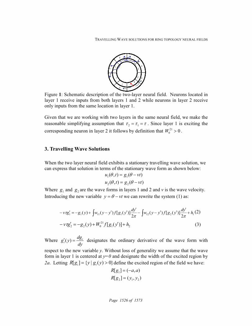
Figure 1: Schematic description of the two
layer 1 receive inputs from both layers 1 and 2 while neurons in layer 2 receive
only inputs from the same location in layer 1.
Given that we are working with two layers in the same neural field,
reasonable simplifying assumption that
corresponding neuron in layer 2 it follows by definition that
3. Travelling Wave Solutions
When the two layer neural field
can express that solution in terms of the stationary wave form as shown below:
Where 1g and 2g are the wave forms in laye
Introducing the new variable
11 )( yggv +−=′− ∫τ
)(22 yggv +−=′− τ
Where dy
dgyg i
i =′ )( designates
respect to the new variable
form in layer 1 is centered at
2a. Letting |][ = gygR i
TRAVELLING WAVE SOLUTIONS FOR RING TOPOLOGY NEURAL F
cription of the two-layer neural field. Neurons located in
layer 1 receive inputs from both layers 1 and 2 while neurons in layer 2 receive
only inputs from the same location in layer 1.
Given that we are working with two layers in the same neural field, we make the
reasonable simplifying assumption that τττ == 12 . Since layer 1 is exciting the
corresponding neuron in layer 2 it follows by definition that 021
0 >W .
Travelling Wave Solutions
When the two layer neural field exhibits a stationary travelling wave solution, we
can express that solution in terms of the stationary wave form as shown below:
)(),(
)(),(
22
11
vtgtu
vtgtu
−=
−=
θθ
θθ
are the wave forms in layers 1 and 2 and v is the wave velocity
Introducing the new variable vty −= θ we can rewrite the system (1) as:
2121112
)]([)(2
)]([)(yd
ygfyywyd
ygfyyw +′
′′−−′
′′− ∫∫ ππ
)]([ 21
21
0 hygfW +′+
designates the ordinary derivative of the wave form with
respect to the new variable y. Without loss of generality we assume that the wave
form in layer 1 is centered at y=0 and designate the width of the excited region by
0)( >ygi define the excited region of the field we have:
),(][
),(][
212
1
yygR
aagR
=
−=
NG TOPOLOGY NEURAL FIELDS
layer neural field. Neurons located in
layer 1 receive inputs from both layers 1 and 2 while neurons in layer 2 receive
we make the
Since layer 1 is exciting the
exhibits a stationary travelling wave solution, we
can express that solution in terms of the stationary wave form as shown below:
wave velocity.
as:
1h+ (2)
(3)
e wave form with
Without loss of generality we assume that the wave
and designate the width of the excited region by
we have:
Page 1526 of 1573

Fayssa Salomon and Evan C Haskell
Where 1y and 2y denote the boundaries of the excited region of layer 2. Since
<<−
= otherwise,0
,1)]([ 1
ayaygf
We can solve (3) explicitly under the boundary condition )()( 22 ππ gg =−
reflecting the periodic nature of the ring topology. The solution is given by:
<≤+
<≤++
−
<≤+
+
=
−
−
−
π
τπτ
τπτ
πτ
τπτ
ττπ
τττπ
ττπ
y
sinh
sinh
ay-
sinh
sinh
-ay- sinh2
sinh
sinh
)(
2
21
0
2
21
0
21
0
2
21
0
2
ahee
v
v
a
W
ahWeee
v
v
a
W
hev
ae
v
v
a
W
yg
v
y
v
v
y
v
a
v
v
y
v
.
In the lateral inhibition neural field model of Amari travelling wave solutions only
exist with positive wave velocity, 0>v [1]. An immediate difference we note
here is that waves may travel with either positive or negative velocity. When the
wave velocity is positive we find that ay −≤≤− 1π and aya ≤≤− 2 yielding the
following solutions for 1y and 2y that depend upon the unknown parameters a
and v. We find 1y and 2y from the relations 0)( 12 =yg and 0)( 22 =yg :
+
−
=
−
ττπτ
τ
τπ
v
aWe
v
v
a
W
hvy
v sinh2
sinh
sinh
ln
21
0
21
0
21
(4)
.
sinh
sinh
ln
21
0
21
0
2
21
02
ττπ
τπτ
τ
v
a
v eWe
v
v
a
W
hWvy
−−
−
−−
= (5)
Page 1527 of 1573

TRAVELLING WAVE SOLUTIONS FOR RING TOPOLOGY NEURAL FIELDS
For a wave with negative velocity we find that aya ≤≤− 1 and π≤≤ 2ya , in
this case 1y will have the same expression as that given for 2y in equation (5)
where the velocity was positive and 2y will have the form:
.
sinh
sinh
ln
21
0
22
τπ
τπτ
τ
ve
v
v
a
W
hvy
−
−
= (6)
From equation (4) and (6) we see that the existence of a travelling wave solution
requires that 02 <h . However the requirement that 02 <h is implicit in equation
(3). If 02 >h then ),[][ 2 ππ−=gR and layer 2 would provide a homogenous
input to layer 1 which would result in a standing wave (v=0) which reduces to
finding a static equilibrium solution to equation (2) [6,7]. Further note that for the
existence of a travelling wave solution equation (5) requires that 2
21
0 hW −> which
we note is also implicitly required by equation (3) in order to have a net excitation
to a neuron in layer 2. When 2
21
0 hW −> we find ∅=][ 2gR which results in a
standing wave solution in layer 1.
Now that we have found ][ 2gR , the excited region in layer 2, we can solve for
)(1 yg . We first let
( )( )
+−
−−+
−−=
′′−−
′′−= ∫ ∫
−
2cos
2sin2)cos()sin(2
2
1
22
1
2)(
2)()(
121212
1
11
1
12
012
11
0
1211
2
1
yyy
yyWyaW
WyyaW
ydyyw
ydyywyK
a
a
y
y
π
π
ππ
so that equation (2) can be rewritten as
)()( 111 hyKyggv ++−=′− τ .
With the periodic boundary condition, )()( 11 ππ gg =− , an explicit solution to
solution to equation (2) is found:
Page 1528 of 1573

Fayssa Salomon and Evan C Haskell
(a) (b)
Figure 2: Waveform of the travelling wave solution. Panel (a) shows the
waveform in layer 1 centered at y=0. Panel (b) shows the corresponding
waveform in layer 2.
( )( )
( )
+−−
+−
−
+−
−+
+
+−
−=
2sin
2cos
2sin
1
1
)sin()cos()sin(
1
1
2)(
121212
1
12
2
11
12
1
12
01211
01
yyyv
yyyW
yy
v
yvyWa
v
hWyy
Wa
yg
τπτ
τπτ
ππ
We can now solve for the unknown width of the excitation region in layer 1, 2a,
and wave velocity, v, from the relations 0)(1 =−ag and 0)(1 =ag .
In figure 2a we show an example of the stationary waveforms for layer 1, )(1 yg ,
for the parameters:
3.0,1,1.0,4,1,4,1 2
21
01
11
1
12
0
11
1
11
0 −==−==−==−= hWhWWWW .
The corresponding waveform in layer 2, )(2 yg , is shown in figure 2b. For this
parameterization we find numerically the width of the waveform in layer 1 is
2a=1.1π, the velocity of the wave velocity is v=0.3π, and for layer two we find
the boundaries of the waveform are located at 1y =-1.03π and 1y =0.50π resulting
in a width of the waveform in layer 2 of 2y - 1y =1.53π.
-pi -pi/2 0 pi/2 pi
-0.4
-0.2
0
0.2
0.4
0.6
0.8
g1(y)
y-pi -pi/2 0 pi/2 pi
-0.4
-0.2
0
0.2
0.4
0.6
0.8
g2(y)
y
Page 1529 of 1573
TRAVELLING WAVE SOLUTIONS FOR RING TOPOLOGY NEURAL FIELDS
4. Discussion
Cortical neurons receive most of their input locally through synaptic interactions
with other neurons that are in close physical proximity. Amari utilized this idea
to develop a model for neural tissue that exhibited both spatial and dynamic
pattern formation[1]. However, VSDI and other experiments have demonstrated
that cortical neurons also possess a topographic map of stimulus feature
space[2,4,9]. The dual constraints of local processing and regular topography of
the cortex have strong influence on neural computation and cortical processing.
Previous studies have shown new results in spatial pattern formation not
previously predicted for neural fields of lateral inhibition type when the
topography implies a compact topology for the neural network [6,7]. In this study
we have built upon this work to introduce a two-layer neural field model in the
ring topology and formulated travelling wave solutions for this model.
Interestingly, with the compact topology there is no restriction on the direction of
motion of the travelling wave as is the case in the two layer lateral inhibition type
neural fields studied by Amari. What we have exhibited in this study is a
mechanism through network interaction that generates and sustains travelling
waves in a ring topology neural field and given explicit solutions for such
travelling waves.
Acknowledgements:
This work has been supported by a Nova Southeastern University President’s
Faculty Research and Development Grant award to ECH.
References:
[1] S. Amari, "Dynamics of pattern formation in lateral inhibition type neural
fields," Biol Cybern, vol. 27, pp. 77-87, 1977.
[2] G. G. Blasdel and G. Salama, "Voltage-Sensitive Dyes Reveal a Modular
Organization in Monkey Straite Cortex," Nature, vol. 321, pp. 579-585,
1986.
[3] Y. Chen, C. R. Palmer, and E. Seidemann, "The relationship between
voltage-sensitive dye imaging signals and spiking activity of neural
populations in primate V1," J Neurophysiol, pp. doi:10.1152/jn.00977.2011 ,
2012.
[4] A. Ginvald and R. Hildesheim, "VSDI: A new era in functional imaging of
cortical dynamics," Nat Rev Neurosci, vol. 5, no. 11, pp. 874-885, 2004.
Page 1530 of 1573
Fayssa Salomon and Evan C Haskell
[5] D. Golomb and G. B. Ermentrout, "Continuous and lurching travelling pulses
in neural networks with delay and spatially decaying connectivity," P Natl
Acad Sci USA, vol. 96, no. 23, pp. 13480-13485, 1999.
[6] E. C. Haskell and P. C. Bressloff, "On the Formation of Persistent States in
Neural Network Models of Feature Selectivity," J Integ Neurosci, no. 2, pp.
102-123, 2003.
[7] E. C. Haskell and V. E. Paksoy, "Localized Activity States for Neuronal
Field Equations of Feature Selectivity in a Stimulus Space with Toroidal
Topology," in Nonlinear and Complex Dynamics: Applictions in Physical,
Biological, and Financial Systems, Jose Antonio Tenreiro Machado, Dumitru
Baleanu, and Albert Luo, Eds. New York: Springer, 2012, pp. 207-216.
[8] K. Kishimoto and S. Amari, "Existence and Stability of Local Excitations in
Homogeneous Neural Fields," J Math Biol, vol. 7, pp. 303-318, 1979.
[9] C. Woolsey, W. H. Marshall, and P. Bard, "Representation of cutaneous
tactile sensibility in the cerebral cortex of the monkey as indicated by evoked
potentials," Bull Johns Hopkins Hosp, vol. 70, pp. 399-441, 1942.
[10] J. Y. Wu, X. Huang, and C. Zhang, "Propagating Waves of Activity in the
Neocortex: What They Are, What They Do," Neuroscientist, vol. 14, no. 5,
pp. 487-502, 2008.
Page 1531 of 1573

Proceedings of the 12th International Conference on Computational and Mathematical Methods in Science and Engineering, CMMSE2012 La Manga, Spain, July, 2-5, 2012
High-Pressure Simulations –
Squeezing the Hell out of Atoms
Peter Schwerdtfeger, Susan Biering, Mustafa Hasanbulli, Andreas Hermann, Jonas Wiebke,
Michael Wormit and Elke Pahl
Centre for Theoretical Chemistry and Physics, The New Zealand Institute for Advanced Study,
Massey University, Auckland, New Zealand
email: [email protected]
Abstract
Fundamental questions are currently explored in our research group concerning the thermodynamic properties of materials under extreme pressure, for example the density-pressure relationship and the equation of state of simple atomic bulk systems (such as the rare gases and mercury) or molecular crystals. The electronic band gap usually decreases with increasing pressure and implications for many-body expansions for electron correlation are discussed. Key words: high pressure, density functional theory, many body expansions
1. Introduction
The pressure range accessible to laboratory experiments exceeds now a remarkable 20 orders of magnitude, from ultra-high vacuum (< 1 nPa) to ultra-high pressures (> 100 GPa). With the development of high-pressure diamond-anvil cells we are now able to study materials at pressures equivalent to the pressure at the centre of our earth (350 GPa). In other planets and stars pressures beyond the TPa range are reached, which can only be explored by thermonuclear explosions or by theoretical methods. At high pressures unusual structures and materials properties are expected such as the metallic state of hydrogen [1]. It is a formidable task to accurately derive equations of state (EOS), f(P,V,T)=0, and corresponding phase diagrams, for gases, liquids and the solid state up to high pressures and temperatures from first principles, that is from quantum theory and statistical physics.
Page 1532 of 1573

HIGH PRESSURE SIMULATIONS
Our research group has recently achieved that for bulk neon, where the isotherms are in excellent agreement with experimental data [2]. The question remains however if the EOS virial equation is applicable for complex systems such as mercury in the gas phase [3]. The accurate determination of melting temperatures up to high pressures remains a challenge even for systems that are well behaved, such as the rare gases [4]. Moving to more complex systems, we present results on optical properties of ice under pressure, which is important for understanding the physics of icy planets such as Neptune [5]. And finally, can we model the melting of mercury using first principle methods? Mercury is a notoriously difficult element to treat by quantum theoretical methods as not only electron correlation effects but also relativistic effects need to be considered, and the many-body expansion of the interaction energy between mercury atoms does not converge in the overlap region of the interaction [6,7].
Figure 1: Optical absorption spectra from many-body GW theory of ice crystals under pressure. Spectra are offset vertically for clarity.
References:
[1] W. Grochala, R. Hoffmann, J. Feng, N. W. Ashcroft, Angew. Chem. Int. Ed. 46, 3620 (2007).
[2] P. Schwerdtfeger, A. Hermann, Phys. Rev. B 80, 064106 (2009). [3] F. Calvo, E. Pahl, P. Schwerdtfeger, F. Spiegelman, J. Chem. Theory
Comput. 8, 639-648 (2012). [4] P. Schwerdtfeger, B. Assadollahzadeh, A. Hermann, Phys. Rev. B 82,
205111 (2010). [5] A. Hermann, P. Schwerdtfeger, Phys. Rev. Lett. 106, 187403 (2011). [6] A. Hermann, R. P. Krawczyk, M. Lein, P. Schwerdtfeger, I. P. Hamilton,
J. J. P. Stewart, Phys. Rev. A 76, 013202-1-10 (2007). [7] B. Paulus, K. Rosciszewski, H. Stoll, N. Gaston, P. Schwerdtfeger, Phys.
Rev. B 70, 165106-1-9 (2004).
Page 1533 of 1573

Proceedings of the 12th International Conference on Computational and Mathematical Methods in Science and Engineering, CMMSE2012 La Manga, Spain, July, 2-5, 2012
GA algorithm for generating geometric random variables of order k
Efraim Shmerling1
1 Department of Computer Sciences and Mathematics
Ariel University Center of Samaria, Ariel 40700, ISRAEL
email: [email protected]
Abstract
We present an algorithm for generating geometric random variables of order k, which is based on approximation of geometric distribution of order k by standard geometric distribution. For this reason the algorithm was named geometric approximation (GA) algorithm. The algorithm is less time-consuming than previously developed universal algorithms for generating random variables with a given probability generating function. The GA random number generator incorporates a random number generator for standard geometric distribution and a generator for finite-valued discrete distributions. Key words: random number generation, discrete distribution, probability generating functions, algorithms, geometric distribution of order k
1. Introduction
Let ,..., 21 XX be a sequence of Bernoulli trials each resulting in either a success
or a failure. Let p and q=1-p denote the probability of success and failure in each
Bernoulli trial, respectively, and let kG denote the waiting time until a sequence
of k consecutive successes are observed for the first time.
kG is called the geometric distribution of order k. Many important results on the
distribution function, generating functions and moments, bounds and approximations, properties, asymptotics, and estimation of geometric variables of order k have been obtained in recent decades (see [1]).
Page 1534 of 1573

GA ALGORITHM
The geometric distributions of order k, in addition to their intricacies and niceties, have assumed special interest in a wide range of areas such as reliability theory, psychology, ecology, molecular biology, meteorology, start-up demonstration testing, statistical quality control and nonparametric statistical inference (see [1, 2]). Despite the widespread dissemination and application of the geometric distribution of order k, random number generators that generate random variables of this type have not yet been developed. While there are universal random number generators that allow one to generate any random variable with a given probability-generating function (see [3]), in many cases utilizing the characteristics of specific random variables makes it possible to develop generators for these variables, which are more efficient than the universal generators. In this paper we demonstrate that this is true for geometric random variables of order k.
2. Description of GA algorithm
In order to present the algorithm we first need to state that for any geometric
random variable kG of order k, an explicit formula for calculating the
probabilities ),()( iGPgkp ki ki can be derived. Since geometric random
variables of order k have rational probability-generating functions that can be
expressed as )(/)()()( * sVsUsPsF , where *P , V and U are polynomials, V
and U don’t have common roots, and the order of V is less than the order of U, the above mentioned formula can be obtained based on a well-known property of random variables with rational probability-generating functions (see [4]).
Let mi ss ,..., designate the distinct zeros of V (real or complex). Let ip designate
the probability that a random variable defined by )(sF takes the value i. All the
probabilities ip with the possible exception of the first few can be expressed as
11
2
2
1
1
1 ...
i
m
m
iiisss
p
.
Here mkk ,1, can be calculated according to the formula )('/)( kkk sVsU .
For example, ),2(gpi 2i , can be expressed as 1
2
2
1
1
1)2(
iiiss
gp
, where
pq
pqqqs
2
42
2,1
,
pqq
q
p
q
p
4
25.05.0
21
, pqq
q
p
q
p
4
25.05.0
22
.
Page 1535 of 1573

GA ALGORITHM
The algorithm presented in this paper requires the utilization of a random number generator for standard geometric random variables and a random number generator for discrete finite-valued random variables. Several random number generators for generating geometric random variables have been developed and included in all mathematical software libraries. Due to the simplicity of geometric distribution, these random number generators are simple and fast. Fortunately, random number generators for discrete finite-valued random variables are also widely available (see [5]). Let G designate a standard geometric random variable with a success probability
in each trial qpk . Let )(gpi designate )( iGP . Comparing the sequences
),(gkpi and ),(gpi ,...2,1i , we note that an integer I can be found such that
)()( 1 gpgkp kii for any i, Iik and )()( 1 gpgkp kii , for any Ii .
We present the proof for the case where 2k , but a completely analogous proof
can be provided for any 2k . For the geometric distribution of order 2 we have the following recursive formula
),2()2()2( 2
2
1 gqppgpgp iii 4i .
Let’s consider a geometric random variable with probability of success in each
trial qp2 . We have 2
21
2 )2()( pgpgpqp , qpgpgpqpqp 2
32
22 )2()()1( ,
qpgpgpqpqp 2
43
222 )2()()1( .
Let *i denote the least integer for which )2()(1** gpgp
ii , 4* i . (Obviously,
such an integer can be found).
We have the following recursive formula for iR , where iR designates
)2(/)2( 1 gpgp ii : ,11
2
1
ii
iRR
qpR ,4i qR 3 , 14 R .
Therefore ,1 2qpRi ,5i from which follows that for any *ij ,
)2()( 1 gpgp jj .
We present a GA algorithm for the case where 2k , but with minimal changes
this algorithm can be converted into a universal algorithm valid for any 2k . The setup stage of the algorithm consists of the following steps.
Step 1 Calculate 1s , 2s , 1 , 2 .
Step 2 Find the smallest index *i , such that )2()( ** 1gpgp
ii
.
Step 3 Build the vector of differences ],...,[12 *
iddD ,
)),()2((/1 1 gpgpKd jjj
1
2
1
*
))()2((
i
e
ee gpgpK , 12 * ij .
The body of the algorithm looks as follows:
Page 1536 of 1573

GA ALGORITHM
Step 1 Generate a random integer RG utilizing a geometric random number generator with input parameter “probability of success in each trial”, which equals
qp2 .
Step 2 If 1* iRG , return 1RG and terminate, else go to step 3.
Step 3 If 1* iRG , generate a random number UNIF with a uniform random number generator and go to step 4.
Step 4 If )(
)2(1
gp
gpUNIF
RG
RG , return 1RG and terminate, else go to step 5.
(According to the property of geometric distribution of order 2 proven above,
)(
)2(1
gp
gp
RG
RG cannot be greater than 1).
Step 5 Utilize a discrete finite-valued random number generator to generate a
random integer RI with possible values 1,...,2 * i , the distribution of which is
defined by the vector of probabilities D. Return RI and terminate.
3. Concluding remarks
1. A random number generator was created based on the above algorithm. It was verified and showed good results in terms of efficiency.
2. The method of geometric approximation presented in the paper can be utilized for creating random number generators for other types of discrete random variables.
References:
[1] N. BALAKRISHNAN, MARKOS V. KOUTRAS, Runs and Scans with Applications, John Wiley &Sons, 2002.
[2] P.S. CHAN, H. K.T. NG, N. BALAKRISHNAN, Statistical inference for start-up demonstration tests with rejection of units upon observing d failures, Journal of Applied Statistics, Volume 35, Issue 8, August 2008, pp. 121-128.
[3] LUC DEVROYE, Algorithms for generating discrete random variables with a given generating function or a given moment sequence, SIAM Journal on Scientific and Statistical Computing, Vol. 12 Issue 1, Jan. 1991, pp. 107-126.
[4] W. FELLER, An introduction to Probability theory and its Applications, third edition, John Wiley &Sons, 1968.
[5] RICHARD A. KRONMAL AND ARTHUR V. PETERSON, On the Alias Method for Generating Random Variables from a Discrete Distribution, The American Statistician, Vol.33, No.4 (Nov.,1979), pp-214-218.
Page 1537 of 1573

Proceedings of the 12th International Conferenceon Computational and Mathematical Methodsin Science and Engineering, CMMSE2012La Manga, Spain, July, 2-5, 2012
Data analysis of photometric observations by HDAC
onboard Cassini: 3D mapping and in-flight calibrations
Yu. Skorov1, R. Reulke2, H. U. Keller1, K.-H. Glassmeier11 Institut für Geophysik und extraterrestrische Physik, Universität
Braunschweig, Germany.2 Institut für Informatik Computer Vision, Humboldt-Universität zu
Berlin, Germany.
emails: [email protected]
AbstractThe hydrogen and deuterium absorption cells (HDAC) are part of the ultraviolet imaging spectrometer [1] onboard the Cassini spacecraft. The absorption cells of HDAC scan the Lyman Alpha emission lines of hydrogen and deuterium atoms. In the photometer mode the absorption cells are not switched on and only the Channel Electron Multiplier (CEM) detector is used to register the signals within a 3 degree field of view (FOV). HDAC in photometer mode was frequently switched on already during cruise to Saturn. The HDAC data set covers 6 years of observations along the spacecraft track from earth to Saturn at 10 AU. By the end of the Cassini mission almost 180° of ecliptic longitude will be covered. The photometer data set together with occasional absorption cell scans will be used to investigate the interstellar hydrogen streaming through the solar system by comparison to existing elaborate models [2].
Key words: data analysis, space physics
IntroductionThe Cassini hydrogen and deuterium absorption cell (HDAC) instrument which was built at the Max-Planck-Institut für Aeronomie consists of a Channel Electron Multiplier (CEM) photo detector equipped with 3 absorption cell filters: a hydrogen cell, a deuterium cell, and an oxygen cell. The hydrogen and deuterium cells function as adjustable absorption filters. The cells are separated by MgF2 windows. HDAC is part of the Cassini ultraviolet imaging spectrometer (UVIS) built by the university of Colorado [1]. In photometer mode HDAC consume little energy and has therefore been often switched on in the background while other instruments lead the observations.
Page 1538 of 1573

DATA ANALYSIS OF HDAC OBSERVATIONS
3D mapping of the Interplanetary Lyman-α background
HDAC has been switched on in photometer mode most of time producing a continuous data set for more than a decade. These observations provide unique views from different positions mostly from outside the hydrogen cavity around the sun. An analysis of the Lyman-α background data serves two purposes: i) determination of the parameters of the interstellar/interplanetary hydrogen, such as its density, flow velocity, and temperature, and ii) determination of the properties of the solar wind, such as the latitudinal dependence of its flux and speed, as well as the solar EUV emission. Here we summarize and map the observations of the interplanetary Lyman-α signal that varies between about 200 to 400 Rayleighs. About sixteen thousand data points were taken during the 7 years of voyage to Saturn where the heliocentric distance varied from 1 to 10 AU. Since orbit insertion in June 2004 observations of the Lyman- α background signal were taken. We display the sight of view (SOV) of the instrument for the last two years (Fig. 1).
In-flight calibrationsThe exhaustive preflight laboratory calibration measurements were done at the Max Planck Institute for Aeronomy and at the Laboratory for Atmospheric and Space Physics in Boulder. The calibrations included: i) evaluation of optical depth versus filament steps; ii) evaluation of instrument spectral sensitivity which is the product of the spectral sensitivity of the detector and the transmission of the windows; iii) evaluation of off-axis response which was measured in the laboratory using 2537nm pen-ray lamp. The detail descriptions of the obtained data can be found in the UVIS calibration report [3].
Fig. 1. The sight of view of the instrument for the two years. The direction from
Page 1539 of 1573

DATA ANALYSIS OF HDAC OBSERVATIONS
the Sun towards Saturn is indicated in each plot. The directions are projected onto the ecliptic plane from the north direction. When the incoming photons reach the HDAC photocathode, the canneltron generates pulses, which is counted within a selected integration period after amplification inside the instrument electronics. Thus the absolute sensitivity of the instrument (that transforms counts to Rayleighs) has to be estimated too. This characteristic as well as all others listed above may change over time due to continuous time degradation of electronics and/or abrupt events. For example, three dramatic sensitivity breakdowns were observed during 2001 (Fig. 2). They were probably caused by the impact of highly energetic particles into the photocathode. Although the channeltron sensitivity eventually recovered for the most part, the pre-flight calibrations for the sensitivity are no more valid. Moreover in-flight analysis of the spectral sensitivity of the far ultraviolet spectrometer onboard Cassini [4] demonstrated that this characteristic may also change with time visibly. Thus the only chance to determine the modern sensitivity of HDAC is to make in-flight comprehensive evaluations of it, e.g. measuring known fluxes from stars or other bodies. Hereafter we present the calibration results based on SPICA and other blue stars observations.
Fig. 2. HDAC photometer data 2001 The HDAC off-axis response was evaluated by the SPICA raster scans. HDAC was programmed to integrate with 0.125 seconds. Star SPICA is blue type star with strong emission in the UV region. Because the counter is only 16bit the maximum number of recognized counts is 216. If an overflow is detected by the counter, then its value is roll over. For the SPICA observations a maximum count rate is up to 500000 counts/sec, thus multiple roll-overs are possible. These corrections can be accomplished automatically and sophisticated data analysis is
Page 1540 of 1573

DATA ANALYSIS OF HDAC OBSERVATIONS
required. During the raster scan several slews are observed in corrected data: each slew shows an increasing signal while SPICA moves towards the FOV center and a decreasing signal while moving outwards. The 2D analysis of the signal structure shown that the off-axis response has visible asymmetric shape, and there are discrepancies between the pre-flight sensitivity curve and the measured off-axis HDAC sensitivity. This instrument characteristic plays important role when we evaluate the absolute sensitivity of HDAC (Counts/sec / Rayleighs). The absolute sensitivity can be determined by comparing the measured count rate of HDAC with the known flux during SPICA observations. The basic equation is
Where I0 is a count rate, SLyα is an absolute value for the sensitivity at Lyman-α, Hλ is a reference spectrum for a specific star, Srel is a relative spectral efficiency curve. The star spectra used in this work was obtained from the INES (IUE Newly Extracted Spectra) database (http://sdc.laeff.inta.es/ines/). We assume that the relative spectral sensitivity is equal to pre-flight calibration. Finally the Lyman-α sensitivity can be determined. The sensitivity of the photomultiplier decreased since insertion of Cassini into Saturn orbit. The current value of 14 count/sec/Rayleighs is still sufficient to provide good signal to noise data (Fig. 3).
Fig. 3. HDAC sensitivity from start to 2012.
Page 1541 of 1573

DATA ANALYSIS OF HDAC OBSERVATIONS
In a future the available data will be re-calibrated taking into account all the observations (and calibration targets) and cross-calibrated with the Lyman- α channel of UVIS (the far ultraviolet spectrometer). This will improve the reliability of both instruments. Once the data set is fully prepared we will compare the observations with models of the hydrogen flow in collaboration with our French colleagues (E. Quemarais). References:
[1] Esposito et al. 2004. Space Sci. Rev., 115, 299. [2] Quémerais et al. 2010. Astrophysical Journal, 711, p. 1257-1262. [3] Cassini UVIS Calibration Report, Draft 2-2, March 15, 2002.[4] Cassini ISS Data User Guide. December 2011.
Page 1542 of 1573

!
"#$%&'()*+,'&%+',+$'&-$*%,.%&#$%)$('/*0'.(1$%+,',0*
2(3$'*%,.%(%1,4$&('3%)012$0*5
"'()*-&-,)/+',6(6-2-&3%()7%$..$1&-8$%&#$'4(2%1,)701&-8-&39!
:09;<,',8=%>9%;1#4-7&=%%?9%@204=%>9%A9%B$22$'
CDEFGFHFIJKLMJNILOPQEGREJSDTJUVFMSFIMMIEFMGSWJXPQEGREYJZIRPDGRSWJ[DG\IMEGFQJLKJ]MSHDERPIG_YJIDTIWEELPDabFMcJdYJeadfghiJ]MSHDERPIG_YJNIMjSDQ
klmnopq!prstsuvwxyzp!
6*&'(1&|k!~mwm!szwmnk~!~xtn!pmk!lnppnsp!ws!slkwp!pwtso!pxkpw!wmw!wk!xokxp!sxwmppn!np!stnnmwk~!tsl!x~kt!wk!pxtmk!m~!np!m!tkpxow!s!nk!pxzonlmwns!m~!mp!~nxpns!wtsx!no!stsxp!nktw!lnktmo!kmtypxtmk!omktp!!|k!wtmpstw!mtmwktnpwnp!s!wnp!tkns!om!nlstwmw!tsok!m~!~kwktlnk!kkwnuk!mp!ts~xwns!s!slkwp!!ktkmwkt!k!tkpkw!tkpxowp!szwmnk~!st!m!n~k!pkw!s!tm~sl!stsxp!lk~nm!kktmwk~!xlktnmoo!k!nukpwnmwk!tsktwnkp!s!wk!omktp!kktmwk~!z!wk!tm~sl!zmoonpwn!~kspnwns!lkws~!m~!wk!tm~sl!tmunwmwnsmo!~kspnwns!lkws~!!zsw!mpkp!m!lss~npktpk!lk~nxl!mp!koo!mp!so~npktpk!lk~nm!mtk!kostk~!st!so~npktpk!lk~nm!k!wkpw!pslk!zny~npktpk!~npwtnzxwnsp!soosk~!z!m!mxppnm!~npwtnzxwns!m~!m!skt!om!~npwtnzxwns!pn!slxwkt!pnlxomwnsp!k!kumoxmwk!wk!umtnsxp!wtmpstw!mtmwktnpwnp!px!mp!stspnw!lkm!tkk!mw!sst~nmwns!xlzkt!m~!swktp!st!moo!spn~ktk~!kmlokp!|kpk!tkpxowp!moos!xp!ws!nltsuk!wk!~kptnwns!s!wk!lmpp!m~!kmw!wtmpstw!n!tm~sl!stsxp!lk~nm!!IQJLMTEJOLMLHEJjITGSYJFMSDEOLMFYJOWSDIFSMQJOPQEGREJ
)&',701&-,)
!pnwx!pmk!szpktumwnsp!tsun~k!pwts!mtxlkwp!wmw!slkwmt!xokn!mtk!
Page 1543 of 1573

!!""# !"$"!! !!%"%""!%!&"""'#'!!'!()#" !!**!!"+"",-." !"'!%%"""#!'!'!!"! !"!""!'!"%"!%%!!/%"0 (1)'",!"""!" !!!!""!/0"!" !!%"$!% !%!!&&/0!"!%2'#""3.4!!'!!!"!"$'(5) !! !""!%%!&6,"'!!%!""%!'!% 7!$"!"'""$(8) '!'!!%"#!!"!"!!%!%! 9!%!!!%'"%$ 6"!'"'" 9%"!%!/:;0!%/<;0! :!!$"
=>?@ABCD?BE@FGAHF
%!:;!'!!2!#'!!!!%!! !!$% 9!!!!!!!
Page 1544 of 1573

!"#!!!$%& &$# '()*+" ###"$#"##& $$%%$###&$$" !"#,+!-./ !"#!$"##
!"#,+-.0/ +12(,"##$(#"$#" !#"($"*" 2345 #"%+#+12 "+62!!(748"+12!!(9:8 ,)(+" 6!"##$,!++! $;(*"!$"#" <*!"=0>(*"!$!($(!##&#=;>(*"!$!!#("=9*(*"!$!!#!##=4>"#"!$1(+)?>"#"!$"$#$(+) #!(+""!"#(0:::::" "($"((#+!"(@+"(% %(++"!!$"",!#!"$#"+#!!!$#!# +!"#$$!A!!B($"!#* (%#"!(+"+ +!++"$#++)( ++%+*"!+"$++" !$#!#+##$!#!+!3;5 (+!#$""##$+!! $!+"# +$+"#+" C"++"#+# !# ##!,!!("# "!(#*"((#+++ ##($$"#(!!!##+"!#)+" !#$<:::::"###%##
Page 1545 of 1573

!"#$%&'&()(%%%*+)*,''*%'%*%'*%''%''*')''*%%%'&-'%'%%')./0/1/23/456789:;,)<"88)=;<)'',!!<,8!>?)7<9@;,)<""A)B'C-'&8,'',!8",<AD)
7!9E,)<"88)''CF+*'*'*'*)'*,<8<,D?G)
7H9F*%'%I*)<"8<'%*'**%*&&&C)'J*,%%*)=C8888)"A!A)
7A9K*,)<"8") %B'*,CLL%+%)&L%'L)
Page 1546 of 1573

Proceedings of the 12th International Conference on Computational and Mathematical Methods in Science and Engineering, CMMSE2012 La Manga, Spain, July, 2-5, 2012
Dynamics of Conformational Modes in Biopolymers
Maria Stepanova1 and Alex Potapov2
1 National Institute for Nanotechnology, National Research Council Canada;
2 Centre for Mathematical Biology, University of Alberta
emails: [email protected], [email protected]
Abstract Key words: soft matter dynamics, proteins, conformation modes
Proteins are major participants of the molecular machinery of life. In this work, we suggest a novel formulation of soft matter theory that paves the way to the understanding of the fundamental “design rules” that determine the structure and function of proteins [1]. Many roles that protein molecules play in the cell are crucially dependent on their structure, which is highly complex and tremendously difficult to understand. Structure of proteins is strikingly different from better-understood substances composed of many similar molecules such as crystals or liquids. In contrast, individual protein molecules generally do not possess a periodic arrangement, are prone to changes in structure (conformation), but also cannot be described as a liquid. In this work, we have devised a rigorous way of representing real-time conformation changes and predicting the properties that remain stable (invariant) in individual protein molecules. The novel framework could be employed to characterize the stable structural properties of proteins from short molecular dynamics simulations. The theory also enables researchers to develop faster, more efficient and robust models for real-time biomolecular structure evolution than those presently available. The outcomes of the work may have profound implications for structural molecular biology, protein engineering, design of new drugs, and curing diseases related to protein misfolding. Examples of the applications are presented. References:
[1] A. POTAPOV AND M. STEPANOVA, Conformational modes in biomolecules: Dynamics and approximate invariance, Phys. Rev. E 85 (2012) 020901(R).
Page 1547 of 1573

Proceedings of the 12th International Conference on Computational and Mathematical Methods in Science and Engineering, CMMSE2012 La Manga, Spain, July, 2-5, 2012
Classification of Workers according to their Risk of Musculoskeletal Discomfort using the K-Nearest
Neighbour Technique
A. Suárez Sánchez1, F.J. de Cos Juez2, F.J. Iglesias Rodríguez1, F. Sánchez Lasheras3 and P.J. García Nieto4
1 Department of Business Administration, University of Oviedo 2 Project Engineering Area, University of Oviedo
3 Department of Construction and Manufacturing Engineering, University of Oviedo
4 Department of Mathematics, University of Oviedo
emails: [email protected], [email protected], [email protected], [email protected], [email protected]
Abstract
K-nearest neighbour (KNN) technique is a widely used classifier because of its simplicity and high efficiency. In this way, this technique was applied in this research work to predict ergonomic disorders with success. This technique was able to classify those workers that have suffered work-related musculoskeletal discomfort in the last twelve months from those that not. According to the model, poor lighting conditions, exposure to vibrations, an uncomfortable chair and a high mental demand are the factors with the strongest influence in the development of this type of health damages. The results of this work can be used as a guide for the implementation of ergonomic solutions. Key words: work, musculoskeletal discomfort, K-nearest neighbour (KNN) technique, categorical variable MSC2000: 62G05; 03C45; 68Q32; 68T05
1. Introduction All around the world, musculoskeletal symptoms and disorders are common amongst working population. This type of work-related health damage can result in serious social impacts on both individuals and communities, and represent a
Page 1548 of 1573

CLASSIFICATION OF WORKERS USING THE KNN TECHNIQUE
considerable economic burden to employers, employees and to society as a whole [1]. According to recent EU figures [2], 24.7% of the European workers complain of backache and 22.8% suffer from muscular pains. Work-related musculoskeletal disorders are usually defined as the diverse types of injuries and pains in muscles, nerves, tendons, ligaments, bones, joints, spinal disks, cartilage, etc. that result from traumatizing the body by demanding more than it is prepared for. It is difficult to compare data from studies of musculoskeletal disorders due to differences in the terminologies used to define this type of complaints. Diverse terms are used in the literature to describe musculoskeletal pain, injury, symptoms, trouble, discomfort and diseases or disorders [3]. To avoid confusion, in this work we have used the term musculoskeletal discomfort (MSD) as defined by Scuffham et al. [3]: musculoskeletal aches, pain, discomfort or numbness affecting an identified body site. Given the importance of musculoskeletal symptoms and disorders, the knowledge of the main factors connected with them is essential in order to minimize their occurrence. Diverse recent works have been published that studied the prevalence of musculoskeletal problems in different occupational groups: computer operators and office workers [4,5], health care workers [6,7], factory and assembly line workers [8], etc. These works usually focus on the risk factors connected to activities developed in the studied professions. On the other hand, a few studies focus on specific groups of factors and try to define their connection to the MSD. For example, Widanarko et al. [9] describe the influence of individual factors such as gender and age, whereas Eatough et al. [10] focus on psychosocial factors. The aim of this work is to develop a holistic model to identify those factors of any kind (individual factors, working conditions, workplace design, etc.) that have a stronger influence on the prevalence of the occupational MSD among the general working population. In this sense, among all supervised learning algorithms, K-nearest neighbour (KNN) algorithm is a widely used classifier because of simplicity and high efficiency [11]. Furthermore, the KNN-based classifier does not require the train stage and is used in this research work with success. From this model, it will be possible to define a musculoskeletal risk profile, as well as to identify the factors that should be controlled to prevent this type of work-related health damage. The results should be taken into account as a guide for the implementation of ergonomic solutions.
2. Materials and methods
2.1. Data set
The data set used in this work records the results of the Sixth Spanish Survey on Working Conditions. This survey was published in 2007 by the Spanish National
Page 1549 of 1573

CLASSIFICATION OF WORKERS USING THE KNN TECHNIQUE
Institute of Safety and Hygiene in the Workplace, a subsidiary body of the Spanish Ministry of Labour and Immigration. The aim of the survey was to provide an overview of the health and safety conditions in Spanish workplaces. The universe consisted of 18,518,444 workers from the entire Spanish territory, employed in all economic activities. Fieldwork was done between December 2006 and April 2007, with personal interviews conducted in the homes of 11,054 workers who responded to a questionnaire consisting of 78 items. For a confidence level of 95.5% and P=Q, the error for the overall sample is ±0.95%. The 78 items in the questionnaire ranged from working conditions to health damage. They were structured in the following groups:
• Labour relation and type of contract. • Information from the company and the working centre. • Type of work and seniority. • Thermal environment. • Physical agents. • Chemical and biological agents. • Safety hazards and conditions. • Workplace design, physical demand and psychosocial factors. • Health and safety management and resources. • Working hours. • Health and safety activities. • Violent behaviour at work. • Work-related accidents and health damage.
In the case of self-reported health damage, the interviewed worker was asked to mention up to eight work-related diseases and symptoms that, from his point of view, he was suffering as a result of his work. These diseases could be selected from a list of 29 offered by the interviewer. The list included six issues that can be classified as musculoskeletal symptoms/disorders: neck pain; back pain; slipped disc; upper limb pain (shoulder, arm, elbow and forearm); wrist, hand and finger pain; lower limb pain (hip, thigh, knee, lower leg, ankle and feet). In order to develop a model to predict the prevalence of the occupational MSD, a new binary variable (P64BINARIA) has been created, which can be considered as the target variable and condenses the information recorded in the group of variables concerning self-reported health damage. This target variable identifies any worker who in the previous year suffered from any of the above-mentioned musculoskeletal symptoms.
2.2. Classification algorithm
Page 1550 of 1573

CLASSIFICATION OF WORKERS USING THE KNN TECHNIQUE
2.2.1. One variable
Consider first the case of only one predictor. The data values 1ix , ni ,...,1= can be written simply 1ix . Each of the ix takes one of 1n categorical values, while each
iy takes one of C class labels. The real number used to replace the data value
ix will be written ( )ixφ . If ix takes the jth category, we also write, in a slight abuse of notation, jφ for the real number associated with that category. So ( )φ is a function that converts the n category labels into n non-unique real numbers: the phrase "the set of φ 's" will refer to "the choice of unique real numbers
1,...,,, 321 nφφφφ ". We write jcN , for the number of observations in class c
belonging to category j: then ∑=+ c jcj NN ,, is the total number of observations in
category j; ∑=+ j jcc NN ,, is the total number of observations in class c; and
nNj c jc =∑ ∑ , . Assume, without loss of generality, that the total sum of ( )ixφ
over all observations, ( )∑ =
n
i ix1φ , is zero. The class c mean of the ( )ixφ is the mean
of all the scalings of observations in class c. Since there are jcN , observations in class c for which the categorical value is j, we can write the class c mean as ( ) ( )∑ =+= 1
1 ,,/1 n
j jjccc NN φφ . Now, the total sum of squares associated with any
particular set of jφ 's is [11]:
( )[ ]∑ ∑= =
+==n
i
n
jjji NxTSS
1 1
2,
21
φφ (1)
while the within-class sum of squares, aggregated over all C classes, is [11]: ( )( ) ( )[ ]∑∑ ∑
= = =+−=−=
C
c
n
j
C
c
cc
cjjc NTSSNWSS
1 1 1
2,
2,
1
φφφ (2)
The set of φ 's yielding the largest ratio WSSTSS / can be found by maximizing TSS under the constraint that WSS be 1. The constraint that WSS be fixed ensures identifiability. Multiplying any set ofφ 's by a constant leaves the ratio of TSS to WSS unchanged. The vector ( )
1,...,, 21 nφφφφ =
r that achieves this is found by the
method of Lagrange multipliers. Some algebra yields the solution as the vector φ and constantλ satisfying [11]:
[ ] 0rrrr
=−− φφλφ UWW (3)or
φμφrr
WU = (4)
Page 1551 of 1573
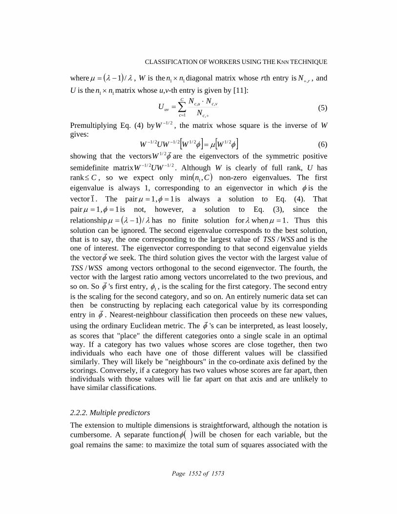
CLASSIFICATION OF WORKERS USING THE KNN TECHNIQUE
where ( ) λλμ /1−= , W is the 11 nn × diagonal matrix whose rth entry is rN ,+ , and U is the 11 nn × matrix whose u,v-th entry is given by [11]:
∑= +
⋅=
C
c c
vcucuv N
NNU
1 ,
,, (5)
Premultiplying Eq. (4) by 2/1−W , the matrix whose square is the inverse of W gives:
[ ] [ ]φμφ 2/12/12/12/1 WWUWW =−− (6)showing that the vectors φ
r2/1W are the eigenvectors of the symmetric positive semidefinite matrix 2/12/1 −− UWW . Although W is clearly of full rank, U has rank C≤ , so we expect only ( )Cn ,min 1 non-zero eigenvalues. The first eigenvalue is always 1, corresponding to an eigenvector in which φ is the vector1
r. The pair 1=μ , 1=φ is always a solution to Eq. (4). That
pair 1=μ , 1=φ is not, however, a solution to Eq. (3), since the relationship ( ) λλμ /1−= has no finite solution forλ when 1=μ . Thus this solution can be ignored. The second eigenvalue corresponds to the best solution, that is to say, the one corresponding to the largest value of WSSTSS / and is the one of interest. The eigenvector corresponding to that second eigenvalue yields the vectorφ
rwe seek. The third solution gives the vector with the largest value of
WSSTSS / among vectors orthogonal to the second eigenvector. The fourth, the vector with the largest ratio among vectors uncorrelated to the two previous, and so on. So φ
r's first entry, 1φ , is the scaling for the first category. The second entry
is the scaling for the second category, and so on. An entirely numeric data set can then be constructing by replacing each categorical value by its corresponding entry in φ
r. Nearest-neighbour classification then proceeds on these new values,
using the ordinary Euclidean metric. The φr
's can be interpreted, as least loosely, as scores that "place" the different categories onto a single scale in an optimal way. If a category has two values whose scores are close together, then two individuals who each have one of those different values will be classified similarly. They will likely be "neighbours" in the co-ordinate axis defined by the scorings. Conversely, if a category has two values whose scores are far apart, then individuals with those values will lie far apart on that axis and are unlikely to have similar classifications.
2.2.2. Multiple predictors
The extension to multiple dimensions is straightforward, although the notation is cumbersome. A separate function ( )φ will be chosen for each variable, but the goal remains the same: to maximize the total sum of squares associated with the
Page 1552 of 1573

CLASSIFICATION OF WORKERS USING THE KNN TECHNIQUE
choice of a particular set of values of φr
, while constraining the within-class sum of squares, aggregated over classes, to be 1. Let the number of categories in the jth variable be jn . Within each variable, categories take the labels jn,...,2,1 for
convenience. No ordering is implied. The total number of categories,∑ =
p
j jn1
, is
written +n . As before, upper-case N's with two subscripts are observation counts: the first subscript names the class the set of observations belongs to, and the second category that the set of observations takes on. So krcN =, is the number of observations in class c for which variable r takes on the value k. +,cN is the number of observations in class c, regardless of category, and lsN =+, is the number of observations in all classes that have a l as their value on variable s. Counts in the cross-tabulation are denoted by separating the categorical variables with an ampersand. Thus, lskrN ==+ &, is the number of observations in all classes with both k as their value for variable r and l as their value for variable s. Write
jnjjj ,1, ,...,φφφ =r
for the vector of real numbers associated with the jn categories in variable j. Then the entire set of parameters to be estimated is
pφφrr
,...,1 , a total of +n real numbers. In a slight abuse of notation, we shall also write ( )ijj xφ
r for the real number corresponding to the category that observation i
has for variable j. The crucial step here is that to keep the dimensionality of the problem manageable, each observation is replaced by the sum of the φ
r's
corresponding to its categorical values. That is, in p dimensions there is the mapping [11]:
( )∑=
→p
jijji xx
1φrr (7)
Of course, the categorical values themselves will in general be correlated across the training set (different variables may measure similar information) so the φ
r's
may be difficult to interpret. This is analogous to the case in multiple regression where the regression coefficients are difficult to interpret when the predictor variables are correlated. Without loss of generality, let the total of all scalings,
( )∑ ∑= =
n
i
p
j ijj x1 1
φ , be 0. Write ( )sI for the indicator function that takes the value 1 when s is true and 0 otherwise. Then the TSS associated with a particular choice of pφφ
rr,...,1 is given by [11]:
( ) ( ) ( )∑∑ ∑∑ ∑= = == =
⎟⎟⎠
⎞⎜⎜⎝
⎛==⎟⎟
⎠
⎞⎜⎜⎝
⎛=
C
c
n
i
p
jijji
n
i
p
jijj xcyIxTSS
1 1
2
11
2
1
φφ (8)
Meanwhile, the within-class sum of squares is [11]:
Page 1553 of 1573

CLASSIFICATION OF WORKERS USING THE KNN TECHNIQUE
( ) ( ) ( )∑∑ ∑∑= = ==
⎟⎟⎠
⎞⎜⎜⎝
⎛−==
C
c
n
i
p
j
cj
p
jijji xcyIWSS
1 1
2
11
φφ (9)
where the class c mean for variable j, for example, is given by [11]:
( ) ( ) ( )+
= =
+
= ∑∑ ==
=,
1 ,,
,
1
c
n
k kjkjc
c
n
i ijjicj N
N
N
xcyI j φφφ (10)
In words, the class c mean for variable j comes from adding up the φ 's for that variable for all the observations that fall in class c, and dividing by the number of observations in that class. Then the within-class-c sum of squares comes from the squared deviations of all those observations' φ 's from that average. The overall WSS is the sum of the within-class sums of squares for all classes. The optimal φ
r
is the one that maximizes WSSTSS / , or equivalently, maximizes TSS while holding WSS equal to 1. The solution is φ
r,λ satisfying:
( ) 0rrr
=−− φλφ UWW (11)or
φμφrr
WU = (12)where W is an ++ × nn block matrix whose s,t block is the ts nn × matrix that is the cross-tab of variables s and t. Similarly, the block stU is the ts nn × matrix whose p, qth element is given by:
[ ] ∑= +
==
⎟⎟⎠
⎞⎜⎜⎝
⎛ −=
C
c c
qtcpsc
pqst N
NNU
1 ,
,, (13)
Once again there is a degenerate solution to Eq. (12) given by 1=μ , 1
rr=φ . This is
not a solution of Eq. (11) and is not of interest. The second eigenvector gives the φr
corresponding to the largest value of WSSTSS / . This −+n vector contains the optimal scalings, one for each category in each variable, with which we replace the categorical values in the data. That operation leaves a numeric data set, to which nearest-neighbour classification with Euclidean metric is applied.
2.2.3. Variable selection
The question of which variables to use is answered by cross-validation. The training set is broken into non-overalapping subsets and the classifier is constructed (that is, the optimal scalings computed) with one subset excluded. The error rate for that classifier on that subset can then be computed. The error rates for each subset are combined into an overall rate. Variables are added sequentially (by selecting the variable yielding the largest increase inλ ) and the model size with the smallest overall error rate chosen. This model size is then used in one additional iteration with the whole training data to find the best set of
Page 1554 of 1573

CLASSIFICATION OF WORKERS USING THE KNN TECHNIQUE
variables. As a practical matter it makes sense to select k, the number of nearest neighbours, at this stage as well.
3. Results The proposed K-nearest neighbour (KNN) algorithm for categorical variables (see Eq. (13)) was applied to the 80% of the data set randomly selected. In our case the mentioned subset was formed by 8,844 instances. Table 1 shows the main algorithm parameters that have been used for the data processing. Table 1. List of main parameters of the algorithm Parameter Value Optimal number of nearest neighbors 47 Number of cross-validations used to find the best model size and number of nearest neighbors
10
Number of knots for numeric variables 10 Number of permutations for variable selection 10 Under these conditions, the set of variables that the algorithm considered as more relevant in order to describe the behavior of the variable P64BINARIA are shown in Table 2. Table 2. List of variables selected by the K-nearest neighbour algorithm for categorical variables Variable Name Variable Description P30_11 Workplace design: poor workplace lighting conditions P18 Exposure to vibration: upper limbs and whole body P30_10 Workplace design: uncomfortable seat P32_5 Mental demand/Psychosocial factors: obliged to pay
attention to various tasks simultaneously P42_1 Working schedule: works on Saturdays P29_2 Second most frequent working posture P34_3 Mental demand/Psychosocial factors: can get external help P70 Gender P16 Workplace humidity level P30_2 Workplace design: patient handling demands P69_ABI Age P28_3 Main accident hazards I P28_2 Main accident hazards II P71 Nationality P27_2 Main accident risk I P30_7 Workplace design: not enough place to work comfortably P28_1 Main accident hazards III P41 Working schedule: flexibility
Page 1555 of 1573

CLASSIFICATION OF WORKERS USING THE KNN TECHNIQUE
The evaluation of the classification capabilities of the model obtained with the variables related in Table 2 was performed with another subset of 2,210 instances corresponding to the 20% of our original sample. Table 3 shows the confusion matrix obtained. Table 3. Confusion matrix Class/recognised As positive As negative Positive 305 ( tp ) 227 ( fn )
Negative 65 ( fp ) 1,613 ( tn )
In order to measure how well the algorithm correctly identifies or excludes the predicted condition, sensitivity, specificity and accuracy metrics have been calculated [12]. Sensitivity and specificity are statistical measurements of the performance of a binary classification test. Sensitivity measures the proportion of actual positives, which are correctly identified, and specificity measures the proportion of negatives, which are correctly identified.
fntp
tpySensitivit
+= (14)
tnfp
tnySpecificit
+= (15)
According to the results of Table 3, the sensitivity obtained by our algorithm was 57.33% and the specificity 96.13%. Finally, in order to assess the overall effectiveness of the algorithm, the accuracy ratio has also been calculated. The value obtained was 86.79%. It was calculated using the following formula:
tnfnfptp
tntpAccuracy
++++
= (16)
4. Discussion In the present work a classification model of workers who suffer from the musculoskeletal discomfort (MSD) has been developed. This model presents high rates of specificity and sensibility. Therefore, it is able to classify correctly most of the workers that answered the survey. As previously mentioned, the set of variables considered by the model as more relevant in order to detect the MSD in workers are those listed in Table 2. A thorough study of these variables leads to their classification in the following groups: workplace design; physical conditions; work demand and organisational factors; individual factors; and workplace hazards and risks. According to the model, workplace design is the most relevant factor to predict the occurrence of the MSD. Variable P30_11 (poor workplace lighting
Page 1556 of 1573

CLASSIFICATION OF WORKERS USING THE KNN TECHNIQUE
conditions) is the one with the strongest influence on the target variable: the most inadequate the lighting, the more frequent the MSD. Apparently, this could be considered a surprising result, as musculoskeletal disorders are more frequently connected to postures or repetitive movements. Despite that it is essential to consider the fact that, when vision is unsatisfactory, the body adapts to a posture aimed at improving it [13]. The lack of a comfortable chair (P30_10) is another important variable, followed from the working in awkward postures, especially bending, crouching and kneeling (P29_2), patient handling (P30_2) and the lack of place to work comfortably (P30_7). The four of them are connected with the well-known effects of adopting bad postures during work and the occurrence of muscular strains and other injuries as a result of over effort or over use. Robertson et al. [5] published a work describing the ergonomic benefits of improving the seat. Furthermore, recent works can be found in the literature that confirm the connection of patient-handling with the MSD [6,7]. The second group in importance are the physical conditions: vibrations and humidity. According to the model (P18), the exposure to hand-arm vibration and, to a lesser extent, whole-body vibration has a strong influence on the occurrence of the MSD. Despite the scarceness of studies, consensus exists for considering vibration as an additional risk factor likely to interact with other work-related musculoskeletal disorder risk factors [14]. Another relevant factor influencing the target variable is humidity (P16): working in a too humid or too dry environment can more frequently lead to suffering the studied disorders than working with the appropriate amount of humidity. There is almost no literature studying this phenomenon (especially the influence of dryness). A possible explanation could be that the lack of humidity leads to dry skin, so that the sensation through the fingertips is reduced and the amount of force used is increased. The third group of factors identified in the model are related to work demands and work organisation. Workers who are obliged to pay attention to various tasks simultaneously (P32_5) and those who cannot get external help (P34_3) are more likely to suffer the MSD, as well as those who frequently work on Saturday (P42_1). These results confirm the well-studied link between psychosocial factors and the MSD. For example, Eatough et al. [10] demonstrate that high levels of psychosocial work stressors are associated with increased employee strain, and this to higher levels of musculoskeletal symptoms. Job satisfaction also appears to have an important influence on this type of disorders. Another very important result is connected to individual factors. According to the model developed, reporting of the MSD is slightly more frequent among males than females (P70). This result contrasts with most of the literature published on this field [4,9], even though a few works [15] stated that males had higher prevalence of certain symptoms compared with females. On the other hand, the connection between age (P69_ABI) and the MSD occurrence (the older the age
Page 1557 of 1573

CLASSIFICATION OF WORKERS USING THE KNN TECHNIQUE
the more frequent the MSD) is consistent with the findings of other studies [16]. Finally, another surprising result of this study (P71) suggests that Spanish workers report the MSD more frequently than immigrant workers. In this case, probably the key word is “report”: the social, legal and work precariousness for most of the latter discourage them from informing about any unease at work. Finally, regarding workplace risks (P27_2, P28_1, P28_2 and P28_3), an interesting connection has been found between the MSD and certain workplace risk factors: too high pace of work, over-efforts, fatigue, unusual tasks or incidents, overwork, etc. Again, this demonstrates that psychosocial factors and mental demand have a key influence on the development of such health damages.
5. Conclusions The present research proposes a KNN-based classification system which is properly adapted to be used with mixed variables (categorical and non categorical). The KNN technique is a flexible classifier which is especially suitable for the musculoskeletal discomfort prediction problem, as in this kind of disorders the independent variables are related with individual and working conditions, and these variables are manifestations of a small number of latent factors. The accuracy of this approach is tested in a real setting which consists of a data set made up of 11,054 workers. The model developed was able to classify those workers that have suffered from musculoskeletal discomfort in the last twelve months from those that not. This research study has shown that KNN technique is able to predict musculoskeletal disorders with more accuracy and effectiveness than other traditional statistical learning techniques. The authors of this work have confidence that the results obtained will be useful to promote new future works in this line developing innovative methodologies in ergonomic disorders prediction. References
[1] M.A. HANSON, K. BURTON, N.A.S. KENDALL, R.J. LANCASTER AND A. PILKINGTON, The Costs and Benefits of Active Case Management and Rehabilitation for Musculoskeletal Disorders (RR 493), Health and Safety Executive Research Report, HSE, Sudbury, 2006.
[2] EUROPEAN AGENCY FOR SAFETY AND HEALTH AT WORK, OSH in figures: Work-related musculoskeletal disorders in the EU - Facts and figures, Publications Office of the European Union, Luxembourg, 2010.
[3] A.M. SCUFFHAM, S.J. LEGG, E.C. FIRTH AND M.A. STEVENSON, Prevalence and risk factors associated with musculoskeletal discomfort in New Zealand veterinarians, Appl. Ergon. 41 (2010) 444–453.
Page 1558 of 1573

CLASSIFICATION OF WORKERS USING THE KNN TECHNIQUE
[4] C. JENSEN, L. FINSEN, K. SOGAARD AND H. CHRISTENSEN, Musculoskeletal symptoms and duration of computer and mouse use, Int. J. Ind. Ergonom. 30 (2002) 265–275.
[5] A. CHOOBINEH, M. MOTAMEDZADE, M. KAZEMI ET AL., The impact of ergonomics intervention on psychosocial factors and musculoskeletal symptoms among office workers, Int. J. Ind. Ergonom. 41 (2011) 671-676.
[6] M. JAWOREK, T. MAREK, W. KARWOWSKI ET AL., Burnout syndrome as a mediator for the effect of work-related factors on musculoskeletal complaints among hospital nurses, Int. J. Ind. Ergonom. 40 (2010) 368–375.
[7] M.H. LONG, V. JOHNSTON AND F. BOGOSSIAN, Work-related upper quadrant musculoskeletal disorders in midwives, nurses and physicians: A systematic review of risk factors and functional consequences, Appl. Ergon. 43 (2012) 455-467.
[8] S.A. FERGUSON, W.S. MARRAS, W.G. ALLREAD ET AL., Musculoskeletal disorder risk during automotive assembly: current vs. seated, Appl. Ergon. 43 (2012) 671-678.
[9] B. WIDANARKO, S. LEGG, M. STEVENSON ET AL., Prevalence of musculoskeletal symptoms in relation to gender, age, and occupational/industrial group, Int. J. Ind. Ergonom. 41 (2011) 561-572.
[10] E.M. EATOUGH, J.D. WAY AND C-H. CHANG, Understanding the link between psychosocial work stressors and work-related musculoskeletal complaints, Appl. Ergon. 43 (2012) 554-563.
[11] S.E. BUTTREY, Nearest-neighbor classification with categorical variables, Comput. Stat. Data An. 28 (1998) 157-169.
[12] L. ÁLVAREZ MENÉNDEZ, F.J. DE COS JUEZ, F. SÁNCHEZ LASHERAS, J.A. ÁLVAREZ RIESGO, Artificial neural networks applied to cancer detection in a breast screening programme, Math. Comput. Model. 52 (2010) 983-991.
[13] J. ANSHEL, Visual Ergonomics Handbook, Taylor & Francis Group, Boca Raton, Florida, 2005.
[14] F. GAUTHIER, D. GÉLINAS AND P. MARCOTTE, Vibration of portable orbital sanders and its impact on the development of work-related musculoskeletal disorders in the furniture industry, Comput. Ind. Eng. 62 (2012) 762–769.
[15] U. AASA, M. BARNEKOW-BERGVIST, K.-A. ANGQUIST AND C. BRULIN, Relationship between work-related factors and disorders in the neck-shoulder and low-back region among female and male ambulance personnel, J. Occup. Health 47 (2005) 481-489.
[16] V.H. HILDEBRANDT, Back pain in the working population: prevalence rates in Dutch trades and professions, Ergonomics 38 (1995) 1283-1298.
Page 1559 of 1573
Proceedings of the 12th International Conference on Computational and Mathematical Methods in Science and Engineering, CMMSE2012 La Manga, Murcia, Spain, 2-5 July 2012
On the Problem of Efficient Search of the Entire Set of Suboptimal Routes in a Transportation Network
Andrey Valuev1,2,3
1 Mechanical Engineering Research Institute named by
A.A.Blagonravov of RAS 2 Moscow State Mining University
3 Moscow Institute for Physics and Technology
email: [email protected]
Abstract
The paper deals with the problem of finding the entire set of acyclic approximate shortest (or quickest) routes with a given value of maximum deviation from the optimum one. An efficient modification of Dijkstra algorithm for an arbitrary connected oriented graph is proposed and substantiated. With a variant of the proposed method the similar to the problem of finding k shortest path may be solved as well. Key words: network, suboptimal route
1. Introduction
The problem of finding approximate optimal routes (with respect to length or time) in any kind of transportation networks has a great practical significance for many reasons. Valuations of times of passing certain arcs may change, some accidents may occur that make some arcs not available for motion for some periods. So a switch to another efficient route possible for the changed situation is needed, and for a wide range of situations the best choice belongs to the set of routes that were suboptimal for the previous estimation of the network state. There may be different set-up of the problem of suboptimal routes. It is more convenient to use the term “length” rather than “time” for weights of arcs and routes, so we shall refer to the problem as the problem of shortest routes. Most attention was given to the problem of finding K shortest routes. Shier’s definition [1] guarantees the existence of K suboptimum lengths (including the optimum one) of routes between two nodes for any case, but these routes may have loops. His double search method produces routes having loops for some values of route length. Reducing the problem to the problem of finding
Page 1560 of 1573

PROBLEM OF SUBOPTIMAL ROUTES IN NETWORK
suboptimum lengths for only acyclic routes, as it was recently proposed by the author [2], it is possible to guarantee determination of all these lengths (and even all corresponding routes) if the number of these lengths does not exceeds K, and, otherwise, exactly K suboptimum lengths. More popular is the method by Yen [3] that practically solves the same problem that in [2]. As to its efficiency, it depends on situations. The method is being modified by many researchers [4, 5] up to recent years, but the main idea of solution of the shortest route problems for a succession (often very long) of networks slightly differing one from another stay the same, and it is the reason for which these methods may not be efficient for all cases. The problem in question is similar to the problem of K shortest routes, but seems more realistic. In fact, some of these routes are useless if their lengths are sufficiently greater then the optimum one. On the other hand, for regular networks we have several routes with the same optimal or almost optimal length, and all them me be useful and must be found. So we propose a maximum deviation from the optimum route length as a criterion for route choice. This kind of problem attracted very little attention, mainly for specific problems [6].
2. The problem set-up and solution method
A network is given with m nodes and n oriented arcs. For a given j-th arc its length is dj. Initial and end number of nodes for the j-th arc are denoted as BEG(j), END(j) and the sets of arcs entering and leaving the i-th node as IN(i), OUT(i), respectively. We shall also define DBEG(j) END(j) as dj.
An arbitrary loopless path between the 1st and another node is a succession
of nodes P=(NODE(1,P), …, NODE(N(P),P)). We will also consider its part P(k:l)=(NODE(k,P),…,NODE(l,P)). LP denotes the route length. The route P obviously determines its final node
i=NODE(N(P),P) (1)
but for our aims it is more convenient to introduce the notation of a marked node as a pair (i,P) for which (1) is valid and to set L(i,P)=LP. The entire set of P
satisfying (1) for a given i is denoted by PS(i). Let Li0=min LP | P PS(i). Our
aim is to establish for each i>1 the set of suboptimal routes PS(i, d)=P PS(i) |
LP Li0+ d The method of the problem solution is modification of the well-known
method by Dijkstra. The main difference is that we work with pairs (i,P) instead of nodes itself, whereas Dijkstra implicitly links with a node the best path P of reaching it. So Dijkstra changes estimates Li for nodes, shifting from a previously known best path to a better one. In our algorithm no change of estimate for (i,P) is
possible, but a pair (i,P) is cancelled if it confirmed that P PS(i, d). As to order of entering marked nodes to the set M0 of finally calculated ones, it is the same as for ordinary nodes in the method by Dijktra. Except (marked) node sets M0 and M1, determined as usually, for each node the switch Si is introduced which value 1
Page 1561 of 1573

PROBLEM OF SUBOPTIMAL ROUTES IN NETWORK
denotes that the value Li0 is just determined. For each i the entire number of pairs
(i,P) M0 M1 is denoted as Ni. For the final state of the set M0,
PS(i, d)=P | (j,P) M0, j=i. (2)
Initial step of the algorithm
Set M1=1, , N1=1. Set Si=0 for each i, Ni=0 for each i>1.
Regular step (k-th iteration)
1. If M1= , halt.
2. Set (s,Q)=arg min L(i,P) | (i,P) M1. If Ss=0, set Ss=1, Ls0=LP . Set
M0=M0 s, M1=M1\s.
3. For each j OUT(s) determine l=END(j) and test whether l NODE(1,Q), …, NODE(N(Q)-1,Q) If not, then:
a. Determine L =LQ+dj. b. If Sl=1, let LMIN=Sl0, otherwise if Nl>0 determine
LMIN=minL(q) | q M2, i(q)=l. If Nl>0, set LMAX=LMIN+ d.
c. If Nl=0 or Nl>0 and L LMAX, then set P=(NODE(1,Q), …, NODE(N(Q)-1,Q), l), N(P)=N(Q)+1, enter (l,P) into M1, set Nl=Nl+1.
d. If L <LMIN, then for all (l,P) M1 for which L(l,P)>L + d exclude (l,P) from M1 and set Nl=Nl-1.
Lemma. Let P PS(i, d), j=NODE(N(P)-1,P)). Then Q=P(1:N(P)-1) PS(j, d).
Proof. Let Q be the shortest path to the j-th node. Then the path
P =(NODE(1,Q ),…,NODE(N(Q ),Q ),i) with length Lj+Dij connects the 1st and
the i-th node. If P does not contain loops, let R=P , otherwise NODE(Q ,k)=i, so
let R=(NODE(1, Q ),…, NODE(Q ,k)); in both cases LR LQ +Dij. Thus Li0 LR
and LP=LQ+Dij Li0+ d LR+ d. So LQ LR-Dij+ d LQ + d, i.e. Q PS(j, d), QED.
Theorem. The proposed algorithm generates the PS(i, d) for all nodes. Proof. The theorem assertion is proved recursively. Let all loopless paths from
the 1st node for which values of LP LNODE(N(P),P) 0+ d are ordered with respect to
LP as P(1),…, P(N). Let i(k)=NODE(N(P(k)),P(k)). It is obvious that for the pair (i(1),P(1)) which enters the set M0 just after
(1, ), the below properties take place: 1) L(i(1),P(1)) is the minimum length of
Lj, j OUT(1), attained at j(1), 2) i(1)=END(j(1)), 3) P(1)=1,i(1). In fact, Lj(1) is the minimum of lengths of all possible paths beginning at the 1
st node. So
L(i(1),P(1))=LP(1). Then, after two algorithm iterations M0=(1, ), (i(1),P(1)).
We suppose that the set M0 after k iterations is (1, ),…, (i(k-1),P(k-1))
and will prove that after (k+1) iterations M0 will be (1, ),…, (i(k),P(k)). As to
P(k) PS(i, d) where i=NODE(N(P(k)),P(k)), we represent it as (1,…,j,i).
According to Lemma, P(k,1:N(P(k))-1) PS(j, d), so P(k,1:N(P(k))-1)=P(k ),
Page 1562 of 1573

PROBLEM OF SUBOPTIMAL ROUTES IN NETWORK
k <k, j=i(k ). Thus, the pair (i(k ),P(k )) entered M0 at the (k +1)-th iteration due to our supposition. According to Step 4, the pair (i(k),P(k)) entered M1 at the same iteration. After that it stayed in M1 till the (k+1) iteration when corresponding value LP(k) becomes the least value for route lengths in M1 and so (i(k),P(k)) leaves M0 and enters M1. To prove this fact we must be sure that no other pair with less values of length may belong to M1 at that moment.
Of course, it may not be a pair (i(l),P(l)) for l>k, since LP(l)>LP(k). Then it
may a pair (j,Q) for which LP(l)>LQ>Lj0+ d. Thus Lj0<LP(k)- d, then Lj0=LQ, and
due to our supposition the pair (j,P) entered M0 as (i(k ),P(k )), k <k. In that case,
however, the pair (j,Q) either was excluded from M1 at the k -th iteration or was not entered into it if it was calculated further. In both case, it may not belong to
M1 after the k -th iteration. So LP(k) was really the minimum route length value for M1. The proof is finished.
3. Remarks on computational efficiency
The most calculation amount for the proposed method make two operations:
minimization of L(i,P) on M1 and testing whether l NODE(1,Q), …, NODE(N(Q)-1,Q). For most efficient implementation of the 1
st one the set M1
must be ordered with B-tree with respect to LP. As to the second operation, it depends on typical values of arc numbers for suboptimal paths. If it is more than 10–20, creation a B-tree on united array of pairs (P, NODE(k,P)) may be useful as well. Results of computational experiments will be presented in the paper presentation on the conference.
References
[1] D.A. SHIER. Iterative Methods for Determining the K Shortest Paths in a Network, Networks, 6 (1976) 205–230.
[2] A.M. VALUEV, The problem of suboptimal routes computation on a network and possibilities of its application to haulage control, Mining informational and analytical bulletin, (2010) Supplement OV5 “Informatization and control”: 52–62 (In Russian).
[3] J.Y.YEN, Finding the k shortest loopless paths in a network, Management Science, 17(1971) 712–716.
[4] J. HERSHBERGER, M. MAXEL, AND S. SURI, Finding the k shortest simple paths: a new algorithm and its implementation, ACM Transactions on Algorithms, 3(2007) 4:45.
[5] Z. GOTTHILF AND M. LEWENSTEIN, Improved algorithms for the k shortest paths and the replacement paths problems, Information Processing Letters 109 (2009) 352–355.
[6] N.S.V. RAO, On fast planning of suboptimal paths amidst polygonal obstacles in plane, Theoretical Computer Science 140 (1995) 265-289
Page 1563 of 1573

Proceedings of the 12th International Conference on Computational and Mathematical Methods in Science and Engineering, CMMSE2012 La Manga, Spain, July, 2-5, 2012
Reactions of Aun+ (n = 1-4) with SiH4 and Finite
Temperature Simulations of Aun (n = 24-40)
James Vey1 and Ian P. Hamilton
1
1 Department of Chemistry, Wilfrid Laurier University, Waterloo, ON,
Canada N2L 3C5
emails: [email protected], [email protected]
Abstract
Key words: gold clusters, scalar relativistic density functional theory
The reactions of gold cluster cations (Aun
+) with silane (SiH4) are studied
theoretically (for n = 1-4) using standard ab initio (density functional theory) methods to obtain minimum energy geometries and thermodynamic quantities (in particular, ΔG values for all reaction channels). For the gold atoms, the Kohn-Sham equations are solved for the valence electrons and scalar relativistic effects are incorporated via a pseudopotential. These reactions have recently been studied experimentally (for n = 1-17) by Jun Miawake and Ko-ichi Sugawara (National Institute of Advanced Industrial Science (AIST), 1-1-1 Higashi, Tsukuba, Ibaraki 305-8565, Japan) using Fourier-transform ion-cyclotron resonance (FT–ICR) mass spectrometry. The gold cluster cations were produced by laser ablation of a gold rod in He atmosphere, and their reactions with silane were observed at room temperature. The experimental results indicate that the main reaction products are loss of H2 to form AunSiH2
+ and loss of 2H2 to form
AunSi+ depending on the cluster size and our calculations support this finding.
Our calculations also show significantly different results for closed-shell (n odd) and open-shell (n even) gold cluster cations. The finite temperature stability of various structural isomers of Aun (n = 24-40) is studied theoretically using a constant temperature ab initio (density functional theory) molecular dynamics method as implemented in the code FHI-aims (Fritz Haber Institute ab initio molecular simulations).[1,2] Here the Kohn-Sham equations are solved for all electrons and scalar relativistic effects are
Page 1564 of 1573

REACTIONS AND STABILITY OF GOLD CLUSTERS
incorporated via the ‘atomic-ZORA (Zeroth Order Regular Approximation)’ approach. Our calculations demonstrate that, at room temperature, the cage structures are significantly more stable than alternate geometries such as the helical nanorod structures that were the subject of a recent theoretical study.[3]
Au24 Cage Structure, 300K, 26ps
Page 1565 of 1573

REACTIONS AND STABILITY OF GOLD CLUSTERS
Au24 Helical Nanorod Structure, 300K, 26ps References:
[1] V. BLUM, R. GEHRKE, F. HANKE, P. HAVU, V. HAVU, X. REN, K. REUTER, M. SCHEFFLER, Ab Initio molecular simulations with numeric atom-centered orbitals, Comp. Phys. Comm. 180 (2009) 2175-2196.
[2] E.C. BERET, L.M. GHIRINGHELLI, M. SCHEFFLER, Free gold clusters: beyond the static, monostructure description, Faraday Discuss. 152 (2011) 153-167.
[3] X.-J. LIU, I. HAMILTON, R. P. KRAWCZYK, P. SCHWERDTFEGER,
The stability of helical gold nanorods: a relativistic density functional study, J. Comp. Chem. 33 (2012) 311-318.
Page 1566 of 1573

Proceedings of the 12th International Conference on Computational and Mathematical Methods in Science and Engineering, CMMSE2012 La Manga, Spain, July, 2-5, 2012
Computer vision algorithmization and intelligent traffic
monitoring
Andrey Vinogradov1
1Moscow Technical University of Communications and Informatics
email: [email protected]
Abstract
Key words: pattern recognition, computer vision, technical
vision, flow monitoring
MSC2000: 68U10, 68U05, 68N15, 68M14
1. Introduction
The matters of algorithmization and applications of machine vision systems are
becoming more and more popular due to the rapid increase in the degree of
electronic vision devices integration in everyday life. Fixed photo and video
cameras, intelligent security TV systems, mobile shooting and recording devices
allow to provide constant monitoring of virtually any necessary object or facility,
to process the received visual and statistic data and to help solve everyday
problems of human life.
One of the main tasks of modern machine vision is monitoring flows in general.
This problem is widely spread and includes such topics as:
-Research of climatic maps;
- Monitoring of pedestrian flows, face recognition, security systems;
- Traffic flow monitoring
etc.
The use of vision systems to monitor traffic flows is one of the most widely used
and common tasks for the implementation of systems of this type. Vehicles are
becoming faster and more powerful, driving conditions – more intense, and the
place of cars in human life - more tangible.
Such claim implementations as the creation of a car “black box”, systems for
synchronization and motion control of other safety systems, suggest the solution
of some basic problems of recognition and computer vision.
Page 1567 of 1573

COMPUTER VISION ALGORITHMIZATION AND INTELLIGENT TRAFFIC MONITORING
Let us consider some of the known problems in this area with known and working
implementations, and their solution methods:
2. Flow recognition and virtual detectors
The general problem statement is to build a map of transport bundles – a field line
analogy – from a sequence of video frames and to automatically place the
controlling detector areas to determine the intensity, velocity, density and other
characteristics of the flow. An important role in frame processing is played by the
depth of the image, because the "price of a pixel" in the processing of frames is
proportional to the distance from the video camera to the source. The processing
of stereo images from several cameras is used to solve this in many papers [1]. In
particular, average intensity values of the detectors located in the bundles -
isolines of the stream are used to reduce error estimates.
Pic. 1. Stereoimage
3. Traffic management elements recognition
This may include a wide range of tasks for implementation. The recognition of
traffic lights, traffic signs, road markings, distance posts along the roadsides and
other repetitive elements of driver notification allow to build a map of the street-
road network as well as to construct intelligent driver assistance systems.
3.1 Traffic lights
There can be two different formulations of the problem, depending on the
practical applications. First is the processing of visual information from a fixed
angle camera. Such a statement makes sense when you are restoring the
Page 1568 of 1573

COMPUTER VISION ALGORITHMIZATION AND INTELLIGENT TRAFFIC MONITORING
information on the work planning of traffic lights. Localization is performed on
the first frame or the first few frames and can be done both in manual and
automatic modes.
The second statement is recognition of traffic lights from a moving vehicle. It is
needed when creating a “black box” and (or) other traffic safety systems.
One of the client-side devices that can be used for traffic light recognition systems
are smartphones with built-in cameras. This type of devices is rapidly developing
in the last years; CPU power, memory size and quality of built-in cameras are
growing fast. The usage of smartphones as a base for client-side applications
allows to conduct the acquisition and processing of data on one device, giving out
data ready for sending to the server (pic. 2).
Pic. 2. An example of monitoring system architecture based on smartphones
(SSSR)
Using smartphones as client devices also allows to reduce the overall price of the
system and increase its scaling, as there are numerous different mobile device
models suitable for solving recognition and monitoring problems. Practically any
of them may be used for creation of computer vision systems.
Specific recognition technologies and realization methods depend on the chosen
smartphones and their operating systems. In particular, for smartphones using the
Google Android operating system the OpenCV program library can be used. It
contains many methods of computer vision adapted for mobile platforms and can
greatly help in the creation of software for recognition systems and save time and
device resources.
The basic process of traffic sign localization and recognition is to find base color
structures on the frame image. Areas that include certain necessary colors are
selected on the image, based on which localization areas can be found.
Color recognition is conducted by transforming the frame from the default RGB
color system to the HSV color system, to increase color determination precision.
Page 1569 of 1573

COMPUTER VISION ALGORITHMIZATION AND INTELLIGENT TRAFFIC MONITORING
During this process the image is transformed from “red-green-blue” color
channels to “hue-saturation-value” color channels. This allows to determine the
exact color by inputting threshold values for each channel.
After that comes the process of clusterization, or selection of connected areas of
each of the recognized colors. Due to this, areas that are too small are excluded
from processing and we can judge of the location of areas of different colors
relative to each other.
The final recognition process consists of evaluating the locations of found areas
and comparing them to the required object’s dimensions. For example, while
localizing traffic lights, the localized area is stretched vertically according to the
found color.
3.2 Traffic signs
There are also at least two approaches. First, data collection of traffic signs
installed in an area, i.e. the creation of the street-road network database and for
the safety of the whole flow. Secondly, the system working in a mobile (moving)
mode in real time, shortest time processing and use for driver assistance and
specific vehicle traffic safety. Localization and recognition are implemented as a
search for areas with a given color structure. In particular, the algorithm of color
image vectorization is used, as implemented in [2] (Pic. 3).
Pic.3. Road sign color vectorization, [2].
As in traffic light recognition, smartphones may be used as client-side devices.
Road sign localization is then made by recognizing connected areas of the same
color on a frame image. The required colors correspond to the main road sign
colors: red, white, blue, black, etc. and their combination. Recognition is
conducted separately for each localized area and can be viewed as determining the
distance between the localized area’s color vector and the color vector of a sign
from the road sign database. This distance is compared to a certain threshold
value. The sign with the minimum distance is viewed as the recognized sign for
this localized area.
The problems of localization and recognition can be separated. For example,
localization can be made on the smartphone, and then the localized areas data can
Page 1570 of 1573

COMPUTER VISION ALGORITHMIZATION AND INTELLIGENT TRAFFIC MONITORING
be sent to the server side for color vectorization, recognition and sign data
storage.
Road sign recognition is a much more complicated and resource intensive task
then traffic light recognition. Thus, not every smartphone can solve this task while
keeping a moderate framerate. The lack of needed computing power makes it
difficult to use smartphones in mobile moving systems and realtime systems,
where a large framerate is needed.
In this case, client-side devices on the base of PTZ dome ip-cameras can be used.
The dome camera connects to a PC with client-side software installed. During
localization the camera can automatically follow the object, panning and zooming
the image with the object’s movement. This allows to conduct localization on a
sequence of frames, increasing the recognition accuracy. Naturally, the processing
of a frame sequence needs more computing power, which should be provided by
the PC connected to the camera.
3.3 Road markings
Road markings as one of the basic and essential element of traffic flow control, is
also a broad and popular field of research. The problem list includes marking state
control, identification of pedestrian crossings and solid lines, classification of
real-time traffic rule violations associated with the intersection of solid lines.
Most papers in this area focus on the recognition of different types of marking
lines, rather than on the assessment of their condition. They use the comparison of
images from the marking line database, for which artificial neural networks are
often used. Most systems allow the detection of elements such as lines of different
types, arrows, signs, pedestrian crossings. Localization technologies often involve
the processing of connected image areas and the use of inverted perspective
images, [3].
Only several papers research the data acquisition of road marking cleanliness state
and the presence of markings in the appropriate places. The vast majority of
works use mobile cameras. These systems exchange information directly with the
marking painting machine one way or another, by communicating it about
necessary work areas, [4] or by controlling the quality of marking placement, [5].
As with the previous tasks, the road markings state can be evaluated using dome
ip-cameras. Their advantage is in being able to automatically track one road
marking line, correcting the camera angle during turns, lane change or other
change of direction. Thus a certain freedom of movement for the driver is
achieved, and recognition errors are reduced.
Tasks such as road marking state, line integrity and necessity of repairs evaluation
can be solved using dome ip-cameras.
Page 1571 of 1573

COMPUTER VISION ALGORITHMIZATION AND INTELLIGENT TRAFFIC MONITORING
4. Vehicle model recognition and driver identification
Undisputable progress was made in the task of vehicle recognition by number in
the recent years. However, there still are some high-speed regimes and climatic
conditions under which the said procedure is unstable. In addition, there are other
reasons for the need to classify cars by model and record the image of the driver.
The status of this problem and its potential solutions are to be discussed.
5. Roadbed state and street-road network landscape compatibility
evaluation
Road contamination in winter can be evaluated to determine the need for
appropriate measures for its clearance. Fixed and hand-held video cameras can
both be used, and neural networks are widely used for information processing,
[6]. Most systems recognize contaminants and irregularities like water, ice and
snow.
In order to construct "lighter" systems the use of low-cost mobile cameras is
allowed. The gradient and RGB properties recognition can then be used, and the
recognized road surface may be automatic classified, [7].
6. Determination of geometric parameters of the road
This task is especially important to create graph road network structures and
various GIS applications. Mobile laboratories with a large number of cameras,
GPS positioning, markings detection and automatic generation of 3D road models
can be used, [8]. Other works use aerial photographs to detect road borders,
intersections, and construct a graph network [9].
Despite the fact that intelligent traffic flow monitoring is a rather extensive area
of modern applied science and widely used area for machine vision systems, this
is not to say that all problems have been resolved in this direction. Although the
general formulation of problems and algorithms may be present, real operating
systems with sufficient accuracy are still scarce.
Many papers describe the improvement and optimization of existing algorithms
described in other papers. All of this gives the right to assert that there is still
considerable room for new developments, algorithms, and in particular, the
practical implementations of monitoring systems in this area.
Page 1572 of 1573

COMPUTER VISION ALGORITHMIZATION AND INTELLIGENT TRAFFIC MONITORING
References:
[1] AUTONOMOUS DRIVING APPROACHES DOWNTOWN U. FRANKE, D.
GAVRILA S. GÖRZIG, F. LINDNER, F. PAETZOLD, C. WÖHLER IEEE
INTELLIGENT SYSTEMS, VOL .13, NR. 6, 1999.
[2] «АВТОМАТИЧЕСКОЕ РАСПОЗНАВАНИЕ СРЕДСТВ
ОПЕРАТИВНОГО УПРАВЛЕНИЯ АВТОДОРОЖНЫМ
ДВИЖЕНИЕМ И ОЦЕНКА ИХ ЭФФЕКТИВНОСТИ»
А.П. БУСЛАЕВ, В.М. ПРИХОДЬКО, В.В. ДОРГАН, Е.А. КРЫЛОВ, В.Ю.
ТРАВКИН, М.В. ЯШИНА, НАУКА И ТЕХНИКА ТРАНСПОРТА 2,
2005
[3] DETECTION AND RECOGNITION OF URBAN ROAD MARKINGS USING
IMAGES PHILIPPE FOUCHER, YAZIDSEBSADJI, JEAN-PHILIPPE TAREL,
PIERRE CHARBONNIER AND PHILIPPE NICOLLE
[4] ROAD MARKINGS RECOGNITION USING IMAGE PROCESSING CHARBONNIER,
P. 9-12 NOV 1997
[5] ROAD MARKINGS RECOGNITION FRANK, D. 16-19 SEP 1996
[6] RECOGNISING GROUPS OF CURVES BASED ON NEW AFFINE MUTUAL
GEOMETRIC INVARIANTS, WITH APPLICATIONS TO RECOGNIZING
INTERSECTING ROADS IN AERIAL IMAGES BARZOHAR, M. 9-13 OCT 1994
[7] WINTER ROAD CONDITION RECOGNITION USING VIDEO IMAGE
CLASSIFICATION KUEHNLE, A BURGHOUT, W DEC 21 1998
[8] ROAD SURFACE CONDITION RECOGNITION METHOD BASED ON COLOR
MODELS LI HONG LIN JUN FENGYANHUI 2009
[9] AN AUTOMATIC IMAGE RECOGNITION SYSTEM FOR WINTER ROAD SURFACE
CONDITION CLASSIFICATION OMER, R. 2010
Page 1573 of 1573

Proceedings of the 12th International Conferenceon Computational and Mathematical Methodsin Science and Engineering, CMMSE 2012July, 2-5, 2012.
A viability analysis for a stock/price model
Chakib Jerry1 and Nadia Raissi2
1 Departement of economy, Faculte des Sciences Juridiques Economiques et Sociales ,University of Moulay Ismail, Meknes, Morocco
2 Departement of Mathematics, Faculty of Sciences, Mohammed V-Agdal University,Rabat, Morocco
emails: [email protected], [email protected]
Abstract
We examine the conditions for the sustainability of a stock/price system based onthe use of a marine renewable resource. Instead of studying the environmental andeconomic interactions in terms of optimal control, we focus on the viability of the system.These viability/crisis situations are defined by a set of economic state constraints. Thisconstraints combine a guaranteed consumption and a minimum income for fishermen.Using the mathematical concept of viability kernel, we reveal that with only economicsconstraints we guarantee a perennial stock/price system.
Key words: Fisheries management, Fishing effort, Demand function, Endogenousprice, Viability kernel
MSC 2000: AMS codes (optional)
1 Introduction
Many bio-economic fishery management problem has already been deal with in the classicalliterature [1, 10, 11, 22, 23]. Often in these works, the main objective was to maximize autility function representing the sustainable economic rent (i.e net economic income). Theresults cannot be realistic due to assumptions under which the models were studied as con-sidering the resource price constant. Also interactions between economic and biological (orecological) dynamics make the problem both interesting and difficult (Wilen[37],Vedeld[35],Bene [3], Hartwick and Olewiler[20]).
c©CMMSE ISBN:978-84-615-5392-1Adendum Page 1574

Template for the CMMSE proceedings
Over the past decades, this topic has received growing attention because many countriesstart to give more interest in environmental issues and also because natural resource ex-ploitation has been shown to be characterized by very frequent ’market failures’ (Tisdell[34],Pearce and Warford[30]). At the moment, Clark’s book[10] is widely considered to be a goodintroduction to the subject. But as we said in our first sentence, many works studying bio-economic models or resource management focus on the maximization of the profit whileneglecting the behavior of the transitory of the resource evolution.
Most economic models addressing the problem of renewable resource exploitation, in-cluding those mentioned above, are built on the frame of a biological model and one of thesimplest models used in population dynamics is the ”logistic model”. When fishing activi-ties are included, the model becomes the Schaefer[33] model. This model is widely used asthe underlying framework by optimal control theory since the latter has been introduced infisheries sciences (see, for instance, Clark[10], Clark and Kirkwood[9], Goh[17], Charles[6],McKelvey[29] and Cohen[13]).
In order to maximize the objective function, one have to follow optimal solutions paths,which are generally unique and do not allow for possible alternate strategies and couldbring undesirable outcomes. Besides in some cases there is undesirable consequences likenegative profits: where the optimal strategy requires closing the fishery for a while (which,practically, implies some fixed costs not taken into account).
All these remarks bring out our interest in addressing the problem from a differentperspective, attempting in particular to take into account ecological and economic issues.The viability approach (Aubin[2]) seems to be a good mathematical framework because itdeals with dynamic systems under state constraints (it correspond to find out an ”invariantdomain” see Clarke et al.[12]). The aim of this method is to analyze the compatibilitybetween dynamics and state constraints. Roughly speaking we search set of controls (ordecisions) that would prevent this system from violating its viability constraints. As theinterest on the interactions between environmental and economic issues is growing in thelast decade also the interest in applying the viability method as a mathematical frameworkarise instead of optimal control. We can mention works of Bene et al. [4], Doyen et al. [14],Rappaport et al. [31], Jerry M. et al.[24] and Jerry C. and Raissi[25, 27]
Well, this work is an attempt to apply this approach to renewable resources managementand especially to fisheries. Here we define the viability from the viewpoint of a governmentthat aims economic and biological sustainability. To achieve this objectif, we may takeinto account in the model constraints of a minimum net benefits and a minimum level ofconsumption of the fish. This constraints are imposed to the state variables which are thecouple stock/price. Moreover, we will show that a single economic constraint ensures bothminimum level of income and stock perenniality. Then, using mathematical concept ofviability kernel (Aubin[2]), we make clear the need to anticipate system dynamics in orderto maintain it viable. Thus situations of overexploitation will be identified in order to avoid
c©CMMSE ISBN:978-84-615-5392-1Adendum Page 1575
jvigo
Resaltado
jvigo
Resaltado
jvigo
Resaltado
jvigo
Resaltado
jvigo
Cuadro de texto

Chakib Jerry, Nadia Raissi
it by setting adaptive regulations. The result of this work contribute to support regulationsof the fishing sector, so it could be submitted to decision-makers.
In this work we describe the dynamics of the system and we identify the viabilityconstraints. The economy sustainability is defined through the viability kernel which isdetermined by
2 The model
Consider a fish stock distributed over a given area that we represent by its density X. Inaccordance with classical modeling [10], the growth of the biomass density is given by:
X = F (X)− qEX, X(0) = X0, (1)
where F (.) is the naturel density growth function, assumed to obey the logistic law (i.eF (.) = vX(1 − X), where v is the intrinsic growth rate of the fish population). E is theharvesting effort such that E ∈ [Emin, Emax] with Emax > Emin > 0 and q stands for thecatchability coefficient.
We introduce to the previous model, the dynamic prevailing on the market in order todetermine endogenously the price[32, 25, 26, 27]
P = ε(D(P )
K− qEX) with P (0) = P0 > 0. (2)
Where, K is the carrying capacity of the area. P is the unit price of the resource. D(P ) isthe demand function, assumed to be strictly nonincreasing and convex[10]. The parameterε stands for the price’s speed adjustment[25, 26, 16, 32].
Then we obtain the following system:
(S)
P = ε(D(P )
K− qEX) with P (0) = P0 > 0,
X = vX(1−X)− qEX, X(0) = X0
(3)
2.1 The sustainability constraints
A second step is to express state variable constraints from a regulating (say a government)agency viewpoint.
The constraint concerns the resource price. First, we consider that the governmentagency seeks to guarantee the sustainability of the fishing activity by maintaining a globalpositive net benefit in the sector at any time[28]. Therefore, P (t) is constrained by a fixedminimum price P
¯, such that
P¯≤ P (t), ∀ t ≥ 0. (4)
c©CMMSE ISBN:978-84-615-5392-1Adendum Page 1576

Template for the CMMSE proceedings
Furthermore, we impose an important requirement related to a guaranteed consumptionlevel throughout time. Then, P (t) is constrained by a fixed maximum price P, such that
P (t) ≤ P, ∀ t ≥ 0 (5)
This price restraint refers to a sustainability and intergenerational equity concern.
Then,as in Jerry and Raissi[25] we thus identify the final constraint,
P¯≤ P (t) ≤ P, ∀ t ≥ 0. (6)
2.2 Definitions and Hypothesis
For the following, it is convenient to posit and to definei. Z := P / P
¯≤ P (t) ≤ P,
ii. I1(E) := X |F (X)− qEX = 0iii. I2(E) := (P,X) | D(P )
K− qEX = 0,
and to assume the following hypothesisH0. v ≥ qEmax.H1. lim
p→∞D(P ) = 0 and lim
p→0D(P ) =∞.
2.3 A viability analysis
A question that arise now is whether the dynamics (6) are compatible and consistent withthe set of constraints Z. In other words, we aim at revealing levels of resource and price ofthe constraint domain Z that are associated with a viable trajectory in Z and thus a viableregulation E(t). To achieve this, we proceed in two steps: identification of viable stationarypoints and determination of viability kernel.
2.3.1 Viable stationary point
The null-clines associated to (S) are defined as follows:
X = 0
P = 0=⇒
X = 0 or X = 1− qE
vP = D−1(KqEX)
. (7)
Then the equilibrium of (S), where the null-clines intersect, is (P ∗, X∗) :
X∗ = 1− qE
vand P ∗ = D−1(KqEX∗) (8)
c©CMMSE ISBN:978-84-615-5392-1Adendum Page 1577
jvigo
Cuadro de texto

Chakib Jerry, Nadia Raissi
Figure 1: The viable stationary point for the system (S)
Let us now study the behavior of (P ∗, X∗) using the linearization method. The Jacobianmatrix J(X,P ), associated to the system (S), reads:
J(X,P ) =
(−2vx+ v − qE 0
−sqE sD′(P )
),where D′(P ) =
∂D(P )
∂P(9)
We know that the behaviour of (P ∗, X∗) depends on the sign of the eigenvalues of J(X,P ),which are:
λ1 = sD′(P )λ2 = −(v − qE)
(10)
We notice that the eigenvalues of J(X,P ) are negative(because of H0 and the fact that thedemand function D(P ) is nonincreasing), then (P ∗, X∗) is a stable node.
In the following theorem, we will establish the global stability of the unique positiveequilibrium (P ∗, X∗) by adopting the Bendixson-Dulac criterion [10]. With the help of thiscriterion we will obtain the nonexistence of a limit cycle which implies that (P ∗, X∗) isglobally asymptotically stable.
Theorem:The nonnegative equilibrium (P ∗, X∗) is globally asymptotically stable.
Proof : To show that (P ∗, X∗) is globally asymptotically stable, it suffices to excludethe existence of a limit cycle in system (S). Let’s consider the following Dulac functionB = 1
X and denote the right hand side of system (S) by G(P,X) and F (P,X), respectively.
(S)
P = ε(D(P )
K− qEX) = G(P,X)
X = vX(1−X)− qEX = F (P,X)(11)
c©CMMSE ISBN:978-84-615-5392-1Adendum Page 1578

Template for the CMMSE proceedings
Then we have∂(BF )
∂X+∂(BG)
∂P= ε
D′(P )
KX− v < 0 (12)
By the Bendixson-Dulac criterion, there is no limit cycle for system (S). Consequently, thepositive equilibrium (P ∗, X∗) is globally asymptotically stable.
2.4 Viability kernel
The next step is to study the whole viability of the system using the concept of viabilitykernel. The viability kernel, denoted by V iab(Z), corresponds to the set of all initialconditions (P,X) such that there exists at least one trajectory starting from (P,X) thatstays in the set of constraints Z. In other words,
V iab(Z) =
(P,X)
∣∣∣∣∣∣∃ an admissible E(.) sucht thatthe solution (P (.), X(.)) of (S),starting from (P,X), is viable in Z
. (13)
First val, let us consider the following sets :
W =P ∗ /∃ X∗ where (P ∗, X∗) is an equilibrium point of (S) and P
¯≤ P ∗ ≤ P
,
H =X∗ /∃ P ∗ where (P ∗, X∗) is an equilibrium point of (S) and P
¯≤ P ∗ ≤ P
.
(14)
We distinguish two situations, depending on the fact that W is empty or not:
Case 1. If W = Ø then V iab(Z) = Ø. This notify that there is no economic state thatmakes possible to satisfy the set of constraint Z. In other words. it means that theeconomic is not sustainable.
Case 2. If W 6= Ø: Before to give the result, let us define and consider the following:
• We define two equilibrium point A∗M (P ∗M , X∗M ) and A∗m(P ∗m, X
∗m), where X∗M =
minX∗H and X∗m = max
X∗H. Also, we define EM and Em which are the correspond-
ing fishing effort respectively to A∗M and A∗m. So, we have EM > Em becauseXM < Xm (see Jerry et al.[24]). Accordingly to the definition of I2(E) we have
D(P )
qKEM<
D(P )
qKEm∀P (15)
This inequality means that ∀E ε [Em, EM ] its corresponding null-cline, i.e: I2(E),is between I2(Em) at the top and I2(EM ) underneath.
• Consider the point (P¯,X
¯), which is the intersection of I2(Em) with the line P = P
¯in the phase plane (P,X).
c©CMMSE ISBN:978-84-615-5392-1Adendum Page 1579
jvigo
Cuadro de texto

Chakib Jerry, Nadia Raissi
• Consider the point (P , X), which is the intersection of I2(EM ) with the lineP = P in the phase plane (P,X).
• We shall consider the curve L1 : ξ 7→ P (ξ) solution of the differential equation
P ′ =
D(P )
k− qEMξ
F (ξ)− qEMξ, with initial condition X. (16)
• Consider the point (P¯,X
¯′), which is the intersection of L1 with the line P = P
¯in the phase plane (P,X).
• We shall consider the curve L2 : ζ 7→ P¯
(ζ) solution of the differential equation
P¯′ =
D(P¯
)
k− qEmζ
F (ζ)− qEmζ, with initial condition X
¯. (17)
• Consider the point (P , X ′), which is the intersection of L2 with the line P = Pin the phase plane (P,X).
V iab(Z) is given by the following propositionProposition:
Under hypothesis H0., one has
V iab(Z) =
(P,X)
∣∣∣∣∣∣P¯′(t) ≤ P ≤ P when X
¯≤ X ≤ X ′
P¯≤ P ≤ P when X ≤ X ≤ X
¯P¯≤ P ≤ P ′(t) when X
¯′ ≤ X ≤ X
(18)
This set is shown by figure 2.
Figure 2: The viability kernel
Proof : The proof of Proposition 1 depends on the position of the initial conditions,indeed:
c©CMMSE ISBN:978-84-615-5392-1Adendum Page 1580

Template for the CMMSE proceedings
1. Consider an initial condition (P0, X0) where P0 < P¯
(t) and X¯≤ X0 ≤ X ′:
The corresponding trajectory will decrease for any fishing effort E ∈ [Em, EM ] untilit cross the curve I2(Em). But before that it will cross the line P = P
¯. This means
that the trajectory won‘t stay in the set of constraint Z. So the choice of the initialcondition must fulfill P
¯(t) ≤ P0 ≤ P .
2. Consider an initial condition (P0, X0) where P¯≤ P0 ≤ P and X
¯≤ X0 ≤ X ′:
The corresponding trajectory will decrease or increase depending on the fact that thepoint (P0, X0) is at the top of I2(Em) or underneath of I2(EM ). In both situationsthe corresponding trajectory stays in the set of constraint Z.
3. Consider an initial condition (P0, X0) where P0 > P (t) and X¯′ ≤ X0 ≤ X:
The corresponding trajectory will increase for any fishing effort E ∈ [Em, EM ] untilit cross the curve I2(EM ). But before that it will cross the line P = P . This meansthat the trajectory won‘t stay in the set of constraint Z. So the choice of the initialcondition must fulfill P
¯≤ P0 ≤ P (t).
Remark:This result shows that by applying an economic condition to the stock/price system, whichis in general the interest of managers and many governments, we maintain an ecological andeconomical sustainability by maintaining the stock greater than a minimum level X
¯′ and
the price at a considerable levels.
3 Conclusion
In this study, we have addressed the problem of the management of natural resource ex-ploitation systems. We re-visit the classical dynamic fishery model introducing the pricedynamics within a new framework based on the concept of viability. The main purpose ofthis new approach is not to maximize an objective function, but to analyze the compati-bility between the dynamics (economic constraints) of a system and its constraints and todetermine the set of controls (or decisions) that prevent the system from violating theseviability constraints. In the present case of a fishery model, management options are iden-tified, assuming a deterministic dynamics (no uncertainty) and a minimum benefit and aminimum consumption guaranteed by the viability constraints. This ability induces ef-fort and biomass minimal thresholds and thus aims at reconciling ecological and economicsrequirements. The viability kernel analysis highlights the need to anticipate the systemdynamics to prevent sector deficits that are related to overexploitation issues. In particular,we distinguish a reversible deficit zone, where the system can recover from crisis and comeback into the viable domain in finite time. Furthermore, we show that with only economics
c©CMMSE ISBN:978-84-615-5392-1Adendum Page 1581
jvigo
Cuadro de texto

Chakib Jerry, Nadia Raissi
requirements, representing by the viability constraint, we ensure an ecological requirementwhich is no more the perenniality of the stock.
References
[1] Ami D., Cartigny P., and Rapaport A., Can Marine Protected Areas EnhanceBoth Economic and Biological Situations?, C. R. Biologies, 328, (2005) 357-366.
[2] Aubin, J.P., Viability Theory. Springer Verlag, Birkhauser, 1991.
[3] Bene, C., Dynamics and adaptation of a fishery system to ecological and economicperturbations: analysis and dynamic modeling, the French Guyana shrimp fishery case,Ph.D. Dissertation, University of Paris VI, Paris, (1997) p. 236 (in French).
[4] Bene, C., Doyen, L., Gabay, D., A Viability Analysis for a Bio-economic model,Cahiers du Centre de Recherche Viabilite-Jeux-Controle, (1998) N 9815.
[5] Bockstael, N.E., Opaluch, J., Discrete modeling of behavioral response under un-certainty: the case of the fishery, J. Environ. Econ. Manage., 10, (1983) 125-137.
[6] Charles, A.T., Optimal fisheries investment under uncertainty, Can. J. Fish. Aquat.Sci., 40, (1983) 2080-2091.
[7] Charles, A.T., Living with uncertainty in fisheries: analytical methods, managementpriorities and the Canadian ground-fishery expe-rience, Fisheries Research, 37, (1998)37-50.
[8] Clark, C.W., The economics of overexploitation, Science, 181, (1973) 630-634.
[9] Clark, C.W., Kirkwood, G.P., Bioeconomic model of the Gulf of Carpentariaprawn fishery, J. Fish. Res. Board Can., 36, (1979) 1303-1312.
[10] Clark C.W., Mathematical Bioeconomics: the Optimal Management of RenewableResources, 2nded.: A Wiley-Interscience, 1990.
[11] Conrad J.M., and Clark C.W., Naturel Resource Economics, Cambridge: Cam-bridge University Press, 1987.
[12] Clarke F. H., Ledyanuv Yu. S., Strem R. J. and Wolenski P. R., Nonsmoothanalysis and optimal control theory, Graduate Texts in Mathematics, Springer, 1998.
[13] Cohen, Y., A review of harvest theory and applications of optimal control theory infisheries management, Can. J. Fish. Aquat. Sci., 44 (Suppl. 2), (1987) 75-83.
c©CMMSE ISBN:978-84-615-5392-1Adendum Page 1582

Template for the CMMSE proceedings
[14] Doyen, L. and Bene, C. , Sustainability of fisheries through marine reserves: arobust modeling analysis, Journal of Environmental Management, 69, (2003) 1-13.
[15] Dubey B., Chandra P. and Sinha P. , A model for fishery resource with reservearea, Nonlinear Analysis: Real world Appl., 4, (2003) 625-637.
[16] Gatto M., and Ghezzi L.L., Taxing Overexploited Open-access Fisheries: The Roleof Demand Elasticities, Ecological Modelling, 80, (1992) 185-198.
[17] Goh, B.S., The usefulness of optimal control theory to biological problem. In: Halfon,E. (Ed.), Theoretical Systems Ecology; Advances and Case Studies. Academic Press,New York, (1979) 385-399.
[18] Gordon, H.S., The economic theory of a common property resource: the fishery, J.Pol. Econ., 82, (1954) 124-142.
[19] Hannesson R., Marine reserves: what would they accomplish?, Mar. Resour. Econ.,13, (1998) 159-170 .
[20] Hartwick, J.M., Olewiler, N.D., The Economics of Natural Resource Use, seconded. Harper and Row, New York, 1998.
[21] Hilborn, R., Ledbetter, M., Analysis of the British Columbia salmon purse-seinefleet: dynamics of movement, J. Res. Board Can., 36, (1979) 384-391.
[22] Jerry M., Raissi N., A policy of fisheries management based on continuous fishingeffort, J. Bio. Sys., 9, (2001) 247-254.
[23] Jerry M., Raissi N., The optimal strategy for a bioeconomical model of a harvestingrenewable resource problem, Math. Comp. Modell., 36, (2002) 1293-1306.
[24] Jerry M., Rapaport A., and Cartigny P., Can protected areas potentially en-large viability domains for harvesting management?, Nonlinear Analysis: Real WorldApplications, 11, (2010) 720-734.
[25] Jerry C. and Raissi N., Impact and effectiveness of marine protected area on eco-nomic sustainability, BIOMAT 2008, Rubem P. Mondaini editor, World Scientific,ISBN: 978-981-4271-81-3, (2008) 182-191.
[26] Jerry C. and Raissi N., Can management measures assure the biological and eco-nomical stabilizability of a fishing model?, Mathematical and Computer Modeling, 51,(2010) 516-526.
[27] Jerry C. and Raissi N., Optimal Exploitation for a Commercial Fishing Model, ActaBiotheoretica, (2012) 1-15.
c©CMMSE ISBN:978-84-615-5392-1Adendum Page 1583
jvigo
Cuadro de texto

Chakib Jerry, Nadia Raissi
[28] Kamili A., These intitule: Bio-economie et Gestion de la Pecherie des PetitsPelagiques- Cas de l’Atlantique Centre Marocain, 2006.
[29] McKelvey, R, Decentralized regulation of a common property renewable resource in-dustry with irreversible investment, J. Environ. Econ. Manage., 12, (1985) 287-307.
[30] Pearce, D.W., Warford, J., World without End. World Bank, Oxford UniversityPress, 1993.
[31] Rapaport A., Terreauxb J.P., Doyen L., Viability analysis for the sustainablemanagement of renewable resources,Mathematical and Computer Modelling, 43, (2006)466-484.
[32] Svizzero S., On the Introduction of Demand in a Fishery Model, 1993.
[33] Schaefer, M.B., Some aspects of the dynamics of populations, Bull. Int. Am. Trop.Tuna Comm., 1, (1954) 26-56.
[34] Tisdell, C.A., Economics of Environmental Conservation Elsevier, Amsterdam,1991.
[35] Vedeld, P.O., The environment and interdisciplinarity,Ecol. Econ., 1 (10) (1994)1-13.
[36] Wilen, J.E., Common property resources and the dynamics of over-exploitation: thecase of the North Pacific fur seal, Research Paper No. 3, Department of Economics,University of British Columbia, Vancouver, 1976.
[37] Wilen, J.E., Bioeconomics of renewable resource use. In: Kneese, A.V., Sweeney,J.L. (Eds.) , Handbook of Natural Resource and Energy Economics, 1 (1993) 61-121Part 1.
c©CMMSE ISBN:978-84-615-5392-1Adendum Page 1584