IV SECTORAL
308
JR GE 13-202 THE REPUBLIC OF KENYA THE PROJECT ON THE DEVELOPMENT OF THE NATIONAL WATER MASTER PLAN 2030 THE REPUBLIC OF KENYA MINISTRY OF ENVIRONMENT, WATER AND NATURAL RESOURCES WATER RESOURCES MANAGEMENT AUTHORITY FINAL REPORT VOLUME - IV SECTORAL REPORT (1/3) OCTOBER 2013 JAPAN INTERNATIONAL COOPERATION AGENCY NIPPON KOEI CO., LTD.
-
Upload
khangminh22 -
Category
Documents
-
view
0 -
download
0
Transcript of IV SECTORAL

THE PRO
JECT ON TH
E DEVELOPM
ENT OF
THE NATIO
NAL WATER M
ASTER PLAN 2030TH
E REPUBLIC OF K
ENYA
JR GE
13-202
THE REPUBLIC OF KENYA
THE PROJECTON
THE DEVELOPMENT OFTHE NATIONAL WATER MASTER PLAN 2030
THE REPUBLIC OF KENYAMINISTRY OF ENVIRONMENT,WATER AND NATURAL RESOURCESWATER RESOURCES MANAGEMENTAUTHORITY
FINAL REPORTVOLUME - IV SECTORAL REPORT (1/3)
OCTOBER 2013
JAPAN INTERNATIONAL COOPERATION AGENCY
NIPPON KOEI CO., LTD.
FINAL REPORT
VOLUM
E - IV SECTORAL REPO
RT (1/3)O
CTOBER 2013

THE PRO
JECT ON TH
E DEVELOPM
ENT OF
THE NATIO
NAL WATER M
ASTER PLAN 2030TH
E REPUBLIC OF K
ENYA
JRGED
13-202
THE REPUBLIC OF KENYA
THE PROJECTON
THE DEVELOPMENT OFTHE NATIONAL WATER MASTER PLAN 2030
THE REPUBLIC OF KENYAMINISTRY OF ENVIRONMENT,WATER AND NATURAL RESOURCESWATER RESOURCES MANAGEMENTAUTHORITY
FINAL REPORTVOLUME - IV SECTORAL REPORT (1/3)
OCTOBER 2013
JAPAN INTERNATIONAL COOPERATION AGENCY
NIPPON KOEI CO., LTD.
FINAL REPORT
VOLUM
E - IV SECTORAL REPO
RT (1/3)O
CTOBER 2013

FINAL REPORT
List of Reports
VOLUME - I EXECUTIVE SUMMARY
VOLUME - II MAIN REPORT (1/2) Part A : Overall Concepts and Frameworks Part B : Lake Victoria North Catchment Area Part C : Lake Victoria South Catchment Area Part D : Rift Valley Catchment Area
VOLUME - III MAIN REPORT (2/2) Part E : Athi Catchment Area Part F : Tana Catchment Area Part G : Ewaso Ng’iro North Catchment Area Part H : Action Plan for WRMA Regional Offices toward 2022
VOLUME - IV SECTORAL REPORT (1/3) Part A : Socio-economy Part B : Meteorology and Hydrology Part C : Water Supply Part D : Sanitation
VOLUME - V SECTORAL REPORT (2/3) Part E : Agriculture and Irrigation Part F : Hydropower Part G : Water Resources Development Part H : Water Resources Management Part J : Flood and Drought Disaster Management
VOLUME - VI SECTORAL REPORT (3/3) Part K : Environmental and Social Considerations Part L : Institution Part M : Database and GIS Part N : Pilot Activities
VOLUME - VII DATA BOOK Part A : Meteorological and Hydrological Data Part B : Irrigation Inventory Part C : Subletting Works
EXCHANGE RATE
US$1.00 = KSh 85.24 = ¥79.98 as of November 1, 2012

Volume – IV Sectoral Report (1/3)
Sectoral Report (A) Socio-economy

Final Report Sectoral Report (A) Socio-economy Table of Contents
Nippon Koei Co., Ltd. A - i The Development of the National Water Master Plan 2030
THE PROJECT ON
THE DEVELOPMENT OF THE NATIONAL WATER MASTER PLAN 2030
IN THE REPUBLIC OF KENYA
FINAL REPORT
VOLUME – IV SECTORAL REPORT (1/3)
A: SOCIO-ECONOMY
Abbreviation
Table of Contents
CHAPTER 1 INTRODUCTION ................................................................................................ A-1
CHAPTER 2 ADMINISTRATIVE DIVISION ......................................................................... A-2
2.1 Geographical Features ......................................................................................................... A-2
2.2 Central Government and Devolved Units ........................................................................... A-2
2.3 Local Government ............................................................................................................... A-3
CHAPTER 3 POPULATION ...................................................................................................... A-4
3.1 Present Conditions of Population ........................................................................................ A-4 3.1.1 Historical Trend of the Population of Kenya ....................................................... A-4 3.1.2 County Distribution ............................................................................................. A-5 3.1.3 Catchment Distribution ........................................................................................ A-5 3.1.4 Urban Population ................................................................................................. A-6
3.2 Population Projection .......................................................................................................... A-6 3.2.1 Base Data ............................................................................................................. A-6 3.2.2 Planning Horizon ................................................................................................. A-7 3.2.3 Population Projection ........................................................................................... A-7
CHAPTER 4 MACRO ECONOMY ......................................................................................... A-10
4.1 Present Economic Performance ........................................................................................ A-10
4.2 GDP Projection ................................................................................................................. A-13 4.2.1 Base Data ........................................................................................................... A-13 4.2.2 GDP Projection .................................................................................................. A-13
CHAPTER 5 PUBLIC FINANCE ............................................................................................ A-15
5.1 Central Government .......................................................................................................... A-15

Final Report Table of Contents Sectoral Report (A) Socio-economy
The Development of A - ii Nippon Koei Co., Ltd. the National Water Master Plan 2030
5.2 Water Sector ...................................................................................................................... A-16
CHAPTER 6 HOUSEHOLD WELFARE AND POVERTY ................................................. A-19
6.1 Household Welfare ............................................................................................................ A-19
6.2 Poverty .............................................................................................................................. A-20
List of Tables
Page Table 2.1.1 Land Area by County in Kenya ............................................................................ A-T-1
Table 2.1.2 Geographical Distribution of County Area by Catchment Area ........................... A-T-2
Table 2.2.1 Inventory of Administrative Units (1/2)-(2/2) ...................................................... A-T-3
Table 2.3.1 List of Local Authorities as of 2012 (1/4)-(4/4) ................................................... A-T-5
Table 2.3.2 Inventory of Local Authorities by Type and By County as of 2012 .................... A-T-9
Table 3.1.1 Population Change, Household Size, and Density in 2009 (1/3)-(3/3) .............. A-T-10
Table 3.1.2 Population Distribution by Catchment and by County in 2009 .......................... A-T-13
Table 3.1.3 1999 Census and 2009 Census Population by County in Urban and Rural Areas ................................................................................................................... A-T-14
Table 3.1.4 Population in Urban Centres in 2009 (1/6)-(6/6) ................................................ A-T-15
Table 3.2.1 Projected Population Distribution by County and Catchment Area in 2030 .................................................................................................................... A-T-21
Table 4.1.1 Gross Domestic Product by Activity/Industry between 2007 and 2011 ............. A-T-22
Table 4.1.2 Wholesale Prices of Major Agricultural Commodities between 2006 and 2012 .................................................................................................................... A-T-23
Table 6.1.1 Percentage Distribution of Household by Main Source of Drinking Water (1/2)-(2/2) ........................................................................................................... A-T-24
List of Figures
Page Figure 1.1.1 Study Flow of Socio-Economy, Economic Evaluation, and Financing
Plan ..................................................................................................................... A-F-1
Figure 2.1.1 Administrative Boundary by County and Catchment Area in 2012 ................... A-F-2
Figure 3.1.1 Population Density by County ............................................................................ A-F-3
Figure 3.1.2 Population in Urban and Peri-urban Centres ...................................................... A-F-4

Final Report Sectoral Report (A) Socio-economy Abbreviations
Nippon Koei Co., Ltd. A - I The Development of the National Water Master Plan 2030
List of Abbreviations and Acronyms
BOPA : Budget Outlook Paper CBS : Central Bureau of Statistics GDP : Gross Domestic Product GIS : Geographic Information System HGF : High Grand Falls JICA : Japan International Cooperation Agency KIHBS : Kenya Integrated Household Budget Survey LAPSET : Lamu Port- Southern Sudan- Ethiopia Transport project LVN : Lake Victoria North LVS : Lake Victoria South MTEF : Medium Term Expenditure Framework MWI : Ministry of Water and Irrigation NIB : National Irrigation Board NWCPC : National Water Conservation and Pipeline Corporation NWMP : National Water Master Plan SAGA : Semi Autonomous Government Agency UN : United Nations WRMA : Water Resource Management Authority WSB : Water Service Board

Final Report Abbreviations Sectoral Report (A) Socio-economy
The Development of A - II Nippon Koei Co., Ltd. the National Water Master Plan 2030
Abbreviations of Measures
Length mm = millimeter cm = centimeter m = meter km = kilometer
Money KSh = Kenya shilling US$ = U.S. dollar
Area ha = hectare m2 = square meter km2 = square kilometer
Energy kcal = Kilocalorie kW = kilowatt MW = megawatt kWh = kilowatt-hour GWh = gigawatt-hour
Volume 1, lit = liter m3 = cubic meter m3/s, cms = cubic meter per second CM = cubic meter MCM = million cubic meter BCM = billion cubic meter m3/d, cmd = cubic meter per day BBL = Barrel
Others % = percent o = degree ' = minute " = second °C = degree Celsius cap. = capital LU = livestock unit md = man-day mil. = million no. = number pers. = person mmho = micromho ppm = parts per million ppb = parts per billion lpcd = litter per capita per day
Weight mg = milligram g = gram kg = kilogram t = ton MT = metric ton Time s = second hr = hour d = day yr = year

NOTE 1. The National Water Master Plan 2030 was prepared based on the material and data provided from
Kenyan Government and its relevant organisations during field surveys in Kenya carried out until November 2012. The sources etc. of the material and data utilised for the study are described in the relevant part of the reports.
2. The names of ministries and related organisations of Kenyan Government are as of November 2012.
3. Information to be updated
The following information which is given in the report is needed to be updated properly:
(1) Information on the proposed development projects
The features and implementation schedules of the proposed development projects may be changed toward implementation of the project. After the subject projects were clearly featured for implementation, the project features and implementation schedules in this report should be updated.
(2) Information on the water demand
The water demand projected in this master plan should be revised when the large scale development plans, other than the projects proposed in this master plan, were formulated, as they will significantly affect to the water resources development and management.
4. Exchange rate for cost estimate
The costs of the proposed development and management plans were estimated by applying the following exchange rate as of November 1, 2012.
EXCHANGE RATE
US$1.00 = KSh 85.24 = ¥79.98 as of November 1, 2012

Final Report Introduction Sectoral Report (A) Socio-economy Chapter 1
Nippon Koei Co., Ltd. A- 1 The Development of the National Water Master Plan 2030
CHAPTER 1 INTRODUCTION
The main objectives of this Master Plan are to provide a policy framework for water resources development based on the updated water balance calculation and establish a sustainable water resource management system in Kenya by 2030. This socioeconomic report aims to present the basic information/data necessary for 1) water demand calculation, 2) calculation of economic evaluation for selected water subsector projects, and 3) estimation of available government budgets for financing the proposed development plans. Figure 1.1.1 shows the workflow of the overall NWMP 2030 and the roles of socioeconomic framework, economic evaluation, and financing plan for formulating the Master Plan. As shown in this figure, this sectoral report is placed as a basis for water demand and water balance calculation, which will then be used for the formulation of each of the water-related development plans. The cost estimate and preliminary economic evaluation for selected projects will be carried out for each development plan, and the overall implementation plan for water resources development will be presented. Based on the implementation plan, a financing plan for each development plan will be performed and located at the final stage of the Master Plan.
In this context, Chapter 1 describes the basis of administrative divisions, by which socioeconomic data are to be distributed. Chapter 2 provides the present and future conditions of the population, while Chapter 3 presents the present economic performance and the gross domestic product (GDP) growth projection up to year 2030, both of which will be used for future water demand analysis. Chapter 4 briefly explains the current public finance at the national level and within the water sector, which will be the basis for examining a financing plan. Chapter 5 summarizes the household welfare, including household expenditure, which will be used for the calculation of the current and future household income in the economic analysis, and the current poverty conditions in Kenya.
Administrative Division Final Report Chapter 2 Sectoral Report (A) Socio-economy
The Development of A - 2 Nippon Koei Co., Ltd. the National Water Master Plan 2030
CHAPTER 2 ADMINISTRATIVE DIVISION
2.1 Geographical Features
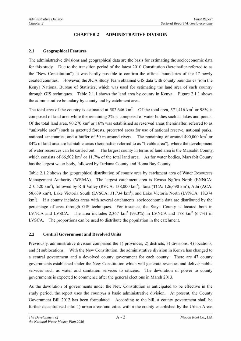
The administrative divisions and geographical data are the basis for estimating the socioeconomic data for this study. Due to the transition period of the latest 2010 Constitution (hereinafter referred to as the “New Constitution”), it was hardly possible to confirm the official boundaries of the 47 newly created counties. However, the JICA Study Team obtained GIS data with county boundaries from the Kenya National Bureau of Statistics, which was used for estimating the land area of each country through GIS techniques. Table 2.1.1 shows the land area by county in Kenya. Figure 2.1.1 shows the administrative boundary by county and by catchment area.
The total area of the country is estimated at 582,646 km2. Of the total area, 571,416 km2 or 98% is composed of land area while the remaining 2% is composed of water bodies such as lakes and ponds. Of the total land area, 90,270 km2 or 16% was established as reserved areas (hereinafter, referred to as “unlivable area”) such as gazetted forests, protected areas for use of national reserve, national parks, national sanctuaries, and a buffer of 50 m around rivers. The remaining of around 490,000 km2 or 84% of land area are habitable areas (hereinafter referred to as “livable area”), where the development of water resources can be carried out. The largest county in terms of land area is the Marsabit County, which consists of 66,502 km2 or 11.7% of the total land area. As for water bodies, Marsabit County has the largest water body, followed by Turkana County and Homa Bay County.
Table 2.1.2 shows the geographical distribution of county area by catchment area of Water Resources Management Authority (WRMA). The largest catchment area is Ewaso Ng’iro North (ENNCA: 210,520 km2), followed by Rift Valley (RVCA: 138,000 km2), Tana (TCA: 126,690 km2), Athi (ACA: 58,639 km2), Lake Victoria South (LVSCA: 31,734 km2), and Lake Victoria North (LVNCA: 18,374 km2). If a county includes areas with several catchments, socioeconomic data are distributed by the percentage of area through GIS techniques. For instance, the Siaya County is located both in LVNCA and LVSCA. The area includes 2,367 km2 (93.3%) in LVNCA and 178 km2 (6.7%) in LVSCA. The proportions can be used to distribute the population in the catchment.
2.2 Central Government and Devolved Units
Previously, administrative division comprised the 1) provinces, 2) districts, 3) divisions, 4) locations, and 5) sublocations. With the New Constitution, the administrative division in Kenya has changed to a central government and a devolved county government for each county. There are 47 county governments established under the New Constitution which will generate revenues and deliver public services such as water and sanitation services to citizens. The devolution of power to county governments is expected to commence after the general elections in March 2013.
As the devolution of governments under the New Constitution is anticipated to be effective in the study period, the report uses the countyas a basic administrative division. At present, the County Government Bill 2012 has been formulated. According to the bill, a county government shall be further decentralised into: 1) urban areas and cities within the county established by the Urban Areas

Final Report Administrative Division Sectoral Report (A) Socio-economy Chapter 2
Nippon Koei Co., Ltd. A- 3 The Development of the National Water Master Plan 2030
and Cities Act 2011, 2) subcounties equivalent to constituencies within the county, and 3) wards within the county. According to the interview with the Ministry of Local Government, previous provinces shall be changed to regions in the future. These decentralised units have been under discussion at the Parliament and have not been established yet. Since these decentralised units have not been effective at the moment, this study uses the previous decentralised administrative units such as division, location, and sublocation, which were described in the 2009 Census. Table 2.2.1 compares the administrative units by county created from the 2009 Census with the 1989 Census (NWMP 1992). In Kenya, administrative divisions have been frequently changed and more administrative divisions have been created since 1989. At the time of the 1989 Census, the number of divisions was 261, however, it has now increased to 634 divisions.
Since the 2009 Census, other statistical data were based on the previous administration division, water demand and time-series data were calculated based on the district level for data consistency.
2.3 Local Government
In urban areas, four autonomous local authorities were established by the “Local Government Act (Chapter 265)”, namely, 1) City Council, 2) Municipal Council, 3) County Council, and 4) Urban Council. According to the 2009 Census, an urban area was defined as “an area with an increased density of human-created structures in comparison to the areas surrounding it and has a population of 2000 and above,” which includes cities, municipalities, town councils and urban councils.
With the New Constitution, the Urban Areas and Cities Act 2011 was enacted in 2012. In this act, two categories on urban areas were created, namely, 1) urban areas which include a municipality and a town and 2) cities. An urban area with a population of at least 500,000 residents is classified as a city, while a municipality comprises a population with more than 250,000, and a town means an urban area with a population of more than 10,000. The act had established three cities, namely, 1) Nairobi, 2) Mombasa, and 3) Kisumu. Nairobi is further classified as a city county. This means that it is a city and also a county. This new classification has been in a transition, but will be effective during the study period. Although the previous urban areas include urban centres with a population of less than 10,000, there is a possibility that the population in these urban centres would increase in the future.
For data consistency, the study uses four types of local authorities used in the 2009 Census, such as 1) City Council, 2) Municipal Council, 3) Town Council, and 4) County Council. Table 2.3.1 shows a list of the local authorities as of 2012, and Table 2.3.2 shows an inventory of local authorities by county. The number of municipal councils and town councils had increased from 28 in 1990 to 41 in 2012 and from 24 in 1990 to 64 in 2012, respectively. These local authorities have the ability to provide public services such as water and sanitation services and health facilities to the citizens.
In rural areas, a county council is an autonomous local authority which provide public services to the population. At present, there are several county councils in each county, partly because it is still in a transition period to establish a county government. The number of county councils had increased from 39 in 1990 to 68 in 2012.
Population Final Report Chapter 3 Sectoral Report (A) Socio-Economy
The Development of A - 4 Nippon Koei Co., Ltd. the National Water Master Plan 2030
CHAPTER 3 POPULATION
3.1 Present Conditions of Population
3.1.1 Historical Trend of the Population of Kenya
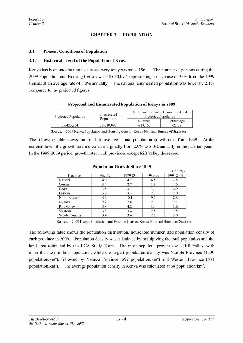
Kenya has been undertaking its census every ten years since 1969. The number of persons during the 2009 Population and Housing Census was 38,610,097, representing an increase of 35% from the 1999 Census at an average rate of 3.0% annually. The national enumerated population was lower by 2.1% compared to the projected figures.
Projected and Enumerated Population of Kenya in 2009
Projected Population Enumerated Population
Difference Between Enumerated and Projected Population
Number Percentage 39,423,264 38,610,097 -813,167 -2.1%
Source: 2009 Kenya Population and Housing Census, Kenya National Bureau of Statistics
The following table shows the trends in average annual population growth rates from 1969. At the national level, the growth rate increased marginally from 2.9% to 3.0% annually in the past ten years. In the 1999-2009 period, growth rates in all provinces except Rift Valley decreased.
Population Growth Since 1969 (Unit: %)
Province 1969-79 1979-89 1989-99 1999-2009 Nairobi 4.9 4.7 4.8 3.8 Central 3.4 2.8 1.8 1.6 Coast 3.5 3.1 3.1 2.9 Eastern 3.6 3.3 2.1 2.0 North Eastern 4.2 -0.1 9.5 8.8 Nyanza 2.2 2.8 2.3 2.1 Rift Valley 3.8 4.2 3.4 3.6 Western 3.8 3.4 2.8 2.5 Whole Country 3.4 3.4 2.9 3.0
Source: 2009 Kenya Population and Housing Census, Kenya National Bureau of Statistics
The following table shows the population distribution, household number, and population density of each province in 2009. Population density was calculated by multiplying the total population and the land area estimated by the JICA Study Team. The most populous province was Rift Valley, with more than ten million population, while the largest population density was Nairobi Province (4509 population/km2), followed by Nyanza Province (599 population/km2) and Western Province (531 population/km2). The average population density in Kenya was calculated at 68 population/km2.

Final Report Population Sectoral Report (A) Socio-economy Chapter 3
Nippon Koei Co., Ltd. A- 5 The Development of the National Water Master Plan 2030
Population, Households, and Density in Each Province
Province Male Female Population Number
Households Number
Land Area (km2)
Density (population/km2)
Nairobi 1,605,230 1,533,139 3,138,369 985,016 696 4,509Central 2,152,983 2,230,760 4,383,743 1,224,742 13,220 332Coast 1,656,679 1,668,628 3,325,307 731,199 82,638 40Eastern 2,783,347 2,884,776 5,668,123 1,284,838 148,994 38North Eastern 1,258,648 1,052,109 2,310,757 312,661 125,806 18Nyanza 2,617,734 2,824,977 5,442,711 1,188,287 9,091 599Rift Valley 5,026,462 4,980,343 10,006,805 2,137,136 181,432 55Western 2,091,375 2,242,907 4,334,282 904,075 8,167 531Whole Country 19,192,458 19,417,639 38,610,097 8,767,954 570,044 68
Note: Land area was calculated by the JICA Study Team as mentioned in Section 1.1, and excluded water bodies. Source: 2009 Population Census, Kenya National Bureau of Statistics; JICA Study Team
3.1.2 County Distribution
The population distribution by county was calculated by integrating the previous districts into counties using information from Statistical Abstract 2011. Table 3.1.1 shows the population distribution, household size, and population density by county in 1999 and 2009. The most populous county in 2009 was Nairobi City County (3,138,369 population), followed by Kakamega County (1,660,651 population) and Kiambu County (1,623,383 population). In terms of population density, Mombasa County has the highest density, accounting for more than 5307 population per km2, followed by Nairobi City County (4509 population/km2) and Nyamira County (950 population/km2). Figure 3.1.1 shows the population density by county.
Among the 47 counties, Mandera County was highest when it comes to family size (8.17 people/household), followed by Wajir (7.47 people/household) and Turkana (6.94 people/household). These counties were also among the low population density areas, accounting for less than 50 population/km2. The average family size in Kenya was estimated at 4.41 people/household.
Due to the frequent change of administrative division in Kenya, it is not reasonable to compare the population growth between the present and previous census. However, the table shows that the population in Mandera County increased from 250,372 in 1999 to 1,025,756 in 2009, whose annual growth rate was calculated at 15.1%. Wajir County, Turkana County, and Bomet County were also seen as counties with growing populations. These counties may have received massive migration from neighbouring counties, which may be the reason for the rapid population increase1.
3.1.3 Catchment Area Distribution
As described in Section 2, the population by county in Kenya was further disaggregated by each catchment area in proportion to the percentage of catchment area. Table 3.1.2 shows the population distribution by catchment area. ACA is the most populous catchment area with a population of 8,979,672. It is followed by LVNCA (8,414,265 population), TCA (6,346,231 population), and LVSCA (6,094,882 population).
1 The results of the 2009 Census has been under review, since the population in North-Eastern and Rift Valley
Provinces near the border has been questioned in the court.

Population Final Report Chapter 3 Sectoral Report (A) Socio-Economy
The Development of A - 6 Nippon Koei Co., Ltd. the National Water Master Plan 2030
3.1.4 Urban Population
As discussed in Chapter 2, urban areas were defined as areas with a population more than 2,000 in the 2009 Census. The 2009 Census provided both the population in urban areas and the population in urban centres, whose total figures are slightly different. Table 3.1.3 compares the urban and rural areas in the 1999 Census and 2009 Census. The urban population in 1999 was calculated by adding the population of urban centres with more than 2,000 people. According to the table, majority of the population in Kenya still resides in rural areas. As of 2009, around 68% of the total population lives in rural areas, whereas around 32% of the total population are located in urban areas. The urban population increased from 9,904,044 in 1999 to 12,487,375 in 2009, but the percentage of population living in urban areas has not changed significantly, estimated at around 32%-33% of the urban population both in 1999 and 2009. Except for Nairobi and Mombasa counties, the most urbanised county is Kiambu County (62%), followed by Kisumu (52%) and Machakos (52%).
As for the urban population in urban centres within urban and peri-urban areas, the urban population was estimated at 11,546,351, accounting for around 30% of the population living in urban centres in 2009. Table 3.1.4 shows the population in urban centres in 2009. As demonstrated in Figure 3.1.2, Nairobi and Mombasa have a population greater than 500,000 in 2009. On the other hand, there are also six urban centres with a population of more than 250,000. Most urban centres are concentrated in highlands and coastal areas. Among the 215 urban centres, 137 urban centres with populations greater than 10,000 were selected as the target areas for urban water supply development plan. In addition, 95 urban centres were selected as the target areas for sewerage development plan.
3.2 Population Projection
3.2.1 Base Data
The latest available information regarding population and its distribution is the 2009 Census. Thus, this study was conducted based on the data of the Census 2009.
Population distribution and composition are one of the most basic pieces of information required in formulating a water resources development plan. There are two main composition categories that are central to the plan, these are urban and rural populations. The split is required in order to assess water supply levels of services in both rural and urban areas as these are distinctly different in Kenya.
There are also two main distribution categories that are critical to development of the plan, namely, spatial distribution by administrative boundary, and spatial distribution by catchment boundary. The former is required for the assessment of the present and future water demands, while the latter is required for calculation of water balance and the water resources development plan.
The 2009 Census does not provide data distributed by counties, therefore, the district boundaries were used. Counties similar with WSBs include multiple districts within their boundaries and therefore redistribution of water demand per county was calculated.
For the water resources development plan, water demand distribution per catchment area and sub-basin are required. Domestic water demand is calculated directly in relation with the population. It was identified that districts were too large compared to the sizes of the sub-basins. Therefore, the

Final Report Population Sectoral Report (A) Socio-economy Chapter 3
Nippon Koei Co., Ltd. A- 7 The Development of the National Water Master Plan 2030
domestic water demand was estimated on the basis of the division population distribution data from the 2009 Census. Catchment distributions employed the ratio method to redistribute the division population and derive water demand into the sub-basins. The methodology to be adopted is described as follows.
If a division falls wholly within a sub-basin boundary, 100% of both urban and rural demands was assigned to that sub-basin. In the case that a division crosses over two or more sub-basins, then (i) the urban demand was allotted as a percentage depending on the urban spread within the sub-basin, and (ii) the rural population was distributed proportionally to the division part area that is included in the sub-basin. Some adjustments were required for urban areas that cross sub-basin boundaries for (i) and areas that are known to have no population for (ii).
3.2.2 Projection Years
The population projection was made for the following years. The target year is 2030 as mentioned in the objective of this study.
Year 2010: Present condition Year 2030: Target year for NWMP 2030 Year 2050: Year to assess the climate change effects on the country’s water resources.
3.2.3 Population Projection
Kenya Vision 2030 presents the future population up to 2032 using the 1999 Census results as the base year. The figure below has been extracted from the Kenya Vision 2030 document. It shows the projected population figures.
19%Urban population%
26% 32% 38% 47% 56% 63% 68%
26.6
20221999
27.1
20172012
22.725.3 26.5
2007 2027
22.3
2032
20.2
2030
24.6
Urban population in millionsRural population in millions
23.1
16.9
5.4 9.012.3
38.243.4
31.7
28.2Total PopulationMillions
34.3 38.8 43.9 49.7 56.2 60.5 63.6
Urban dwellers exceed half the country’s population and overtake rural dwellers
Note: * Based on projections from 1999 National Census Source: CBS
Population Projection by Kenyan Vision 2030
The complete results of the 2009 Census were not available at the time of this analysis, but the census report highlights some anomalous results in eight districts. From the report, the data indicating the rate of increase is higher than the population dynamics (births, deaths, etc.). Age and sex profiles

Population Final Report Chapter 3 Sectoral Report (A) Socio-Economy
The Development of A - 8 Nippon Koei Co., Ltd. the National Water Master Plan 2030
deviate from the norm and significant growth is observed in household size without the accompanying growth in number of households (refer to 2009 Census). Eight anomalous districts were extracted and their population results were compared with the results from the 1999 Census projected to 2009, using the Kenya Vision 2030’s growth rates.
Correction of 2009 Census Population
Districts 2009 Census Population
1999 Census Population Projected in 2009*
Difference
Lagdera 245,123 207,966 37,157 Wajir East 224,418 145,964 78,454 Mandera (Central, East, West) 1,025,756 321,062 704,694 Turkana (Central, North, South) 855,399 564,075 291,324
Note: * Based on Kenya Vision 2030’s growth rates Source: JICA Study Team based on Census 2009 data and Kenya Vision 2030
Based on the 1999 Census projected to 2009, Mandera should have a total population of 321,062 as opposed to 1,025,756. The difference is 704,694 people. Similarly, Turkana has a difference of 291,324, while Lagdera 37,157, and Wajir East 78,454. The total difference is 1.112 million. This indicates that the 2009 Census population should be approximately 38.61 – 1.112 = 37.5 million, which closes the gap with Kenya Vision 2030.
Following this correction, the 2009 Census population is still ahead of Kenya Vision 2030 but it is believed that the residual difference is probably due to an underestimation of the Kenya Vision 2030 projection. Based on information from MWI, the family planning policies have not been effective in the last decade and an increase in birth rates has been observed. It is expected that the policies will be more efficient in the future and birth rates are expected to fall. Based on this information and assumptions, the study adopts the 2009 Census data as the base year. Adjustments on the anomalies in the eight districts were made and the resulting data were projected based on Kenya Vision 2030’s growth rates presented below.
Note: Projections for 2010 and 2011 utilised yearly growth rates calculated from
Kenya Vision 2030 Source: Kenya Vision 2030
Average Population Growth Rate in Kenya Vision 2030
Projections beyond 20 years are not available and are very difficult to predict. The United Nations projects the population to be 96.89 million by 2050, which is the indicative figure for this study. The

Final Report Population Sectoral Report (A) Socio-economy Chapter 3
Nippon Koei Co., Ltd. A- 9 The Development of the National Water Master Plan 2030
population for the period between 2030 and 2050 is projected to increase at an average annual growth rate of 1.94%, indicating a more developed country with a decrease in birth rates and a reduction in internal migration rates from rural to urban.
The table below summarizes the national population projected based on the procedure mentioned above. Table 3.2.1 shows the projected population distribution by county and catchment area in 2030.
Projected Population (Unit: million persons)
Year 2009 (Census)* 2010 2030 2050 Area No. % No. % No. % No. %
Urban 12.29 32.8 13.08 33.9 46.02 67.8 65.69 67.8 Rural 25.11 67.2 25.45 66.1 21.82 32.2 31.20 32.2 Total 37.40 100 38.53 100 67.84 100 96.89** 100
Note: * 2009 Census population adjusted for eight anomalous Districts
** UN World Urbanization Prospects: The 2011 Revision
Source: JICA Study Team based on Kenya Vision 2030 and UN projection

Macro Economy Final Report Chapter 4 Sectoral Report (A) Socio-economy
The Development of A - 10 Nippon Koei Co., Ltd. the National Water Master Plan 2030
CHAPTER 4 MACRO ECONOMY
4.1 Present Economic Performance
In the past, the economy of Kenya has been largely dependent on agriculture and tourism. According to the 2012 Economic Survey, Kenya continues to recover steadily from the multiple shocks that the country suffered since 2008. The World Bank’s Kenya Economic Update for June 2012 projected a GDP growth rate of 5.0% in 2012, while the government estimated at the same level at 5.2%. The following table shows macroeconomic indicators between 2007 and 2011.
Kenya is one of the most industrially developed countries in East Africa. Yet, the manufacturing sector accounts only for 9.4% of the GDP. Economic development in recent years can be attributed to expansions in the tourism, telecommunications, transport, and construction sectors, as well as the recovery in agriculture. Agriculture (including coffee and tea cultivation) is the main source of revenue for around 70% of the population in Kenya. In addition, this sector, which is around 24% of the GDP, is still seen as the largest contributor to the Kenyan economy. This is followed by the transport and communications sectors, contributing to 9.7% of the GDP in 2011. The energy subsector consists of 0.9% of the GDP on average in the past five years, while the water supply subsector contributes to 0.7% of the GDP in 2011. The tourism sector has also been growing in recent years, comprising around 17% of export earnings2. The GDP per capita has been increasing steadily, accounting for US$774 in 2011. Kenya is considered to be on the path to reach a lower middle-income status (US$1,000). Table 4.1.1 shows the GDP by activity/industry between 2007 and 2011.
Economic Statistics
Item 2007 2008 2009 2010 2011* GDP (current price- Ksh) (billions) 1,834 2,108 2,367 2,550 2,671 GDP growth (annual %) 7.0 1.5 2.7 5.8 4.4 Inflation (annual %) 4.3 16.2 10.5 4.1 14.0 GDP by Selected Sectors
Agriculture, value added (% of GDP) 21.7 22.3 23.5 21.4 24.0 Manufacturing (% of GDP) 10.4 10.8 9.9 9.9 9.4 Electricity and Water Supply 1.5 2.1 1.9 1.4 0.9
Electricity (% of GDP) 0.8 1.5 1.2 0.7 0.2 Water Supply (% of GDP) 0.6 0.6 0.6 0.7 0.7
Transport and communications (% of GDP) 10.6 10.3 9.9 10.0 9.7 Hotels and restaurants (% of GDP) 1.6 1.1 1.7 1.7 1.7
GDP growth rate by selected sectors Growing of crops and horticulture (growth rate %) 2.7 -7.2 -5 7.5 0.0 Electricity (growth rate %) 11.8 6.1 5.2 11.9 -4.5 Water Supply (growth rate %) 1.8 2.9 3.6 3.5 3.2
GDP per capita (US$) 719 774 738 760 774 Balance of trade (KSh billion) -330 -426 -443 -537 -805 Note: * Provisional Source: Economic Survey 2012; Kenya Economic Update June 2012, World Bank
2 Kenya Economic Update, June 2012.
Final Report Macro Economy Sectoral Report (A) Socio-economy Chapter 4
Nippon Koei Co., Ltd. A- 11 The Development of the National Water Master Plan 2030
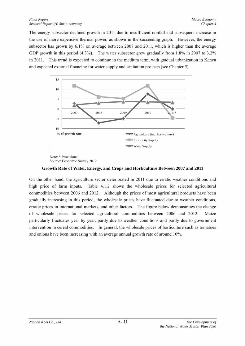
The energy subsector declined growth in 2011 due to insufficient rainfall and subsequent increase in the use of more expensive thermal power, as shown in the succeeding graph. However, the energy subsector has grown by 6.1% on average between 2007 and 2011, which is higher than the average GDP growth in this period (4.3%). The water subsector grew gradually from 1.8% in 2007 to 3.2% in 2011. This trend is expected to continue in the medium term, with gradual urbanization in Kenya and expected external financing for water supply and sanitation projects (see Chapter 5).
-10
-5
0
5
10
15
2007 2008 2009 2010 2011*
% of growth rate Agriculture (inc. horticulture)
Electricity Supply
Water Supply
Note: * Provisional Source: Economic Survey 2012
Growth Rate of Water, Energy, and Crops and Horticulture Between 2007 and 2011
On the other hand, the agriculture sector deteriorated in 2011 due to erratic weather conditions and high price of farm inputs. Table 4.1.2 shows the wholesale prices for selected agricultural commodities between 2006 and 2012. Although the prices of most agricultural products have been gradually increasing in this period, the wholesale prices have fluctuated due to weather conditions, erratic prices in international markets, and other factors. The figure below demonstrates the change of wholesale prices for selected agricultural commodities between 2006 and 2012. Maize particularly fluctuates year by year, partly due to weather conditions and partly due to government intervention in cereal commodities. In general, the wholesale prices of horticulture such as tomatoes and onions have been increasing with an average annual growth rate of around 10%.

Macro Economy Final Report Chapter 4 Sectoral Report (A) Socio-economy
The Development of A - 12 Nippon Koei Co., Ltd. the National Water Master Plan 2030
0
500
1,000
1,500
2,000
2,500
3,000
3,500
4,000
4,500
2006 2007 2008 2009 2010 2011 2012
Ksh
Banana
Cabbages
Maize Dry
Onion
Tomato
Note: Annual average price, except for the price in 2012 as of November 1, 2012 Source: Economic Review of Agriculture 2012; Business Daily, November 2, 2012
Wholesale Prices of Major Agricultural Commodities Between 2006 and 2012
East Africa is the second highest growing region in the world and Kenya is taking advantage of its location. Trade with East African countries has been rapidly growing in the past five years (annual growth rate of around 19% in export). Kenya serves as a regional hub to cater the service and finance industries in East Africa. Kenya’s neighbouring countries, Tanzania and Uganda, have a surplus in agriculture and they have recently discovered gas and oil which boosted its economy. Kenya’s export earnings from Uganda consists of around 15% of the total, which is the highest among other of Kenya’s export destinations. The development of the Northern Corridor and the Lamu Port-Southern Sudan-Ethiopia Transport Project (LAPSET) which would connect Lamu Port to Southern Sudan and Ethiopia is expected to enhance the growth in the transport sector and trade among countries. In the water sector, a water supply project for transferring water from the High Grand Falls (HGF) to the Lamu area, and an energy generation project from the HGF have been planned as part of the LAPSET.
Kenya’s Export by Destination, 2007-2011 (Unit: KSh million)
Destination 2007 2008 2009 2010 2011 % of Total in 2011
Growth (July 2011)
Europe Total 79,277 98,513 100,975 109,422 134,959 26% 14%America Total 20,520 22,054 18,961 24,380 27,491 5% 8%Africa Total 124,029 162,541 162,732 188,914 247,601 48% 19%South Africa 2,347 3,641 3,580 2,444 2,835 1% 5%Rwanda 5,801 8,953 9,536 10,535 13,555 3% 24%Egypt 9,111 15,490 11,885 18,116 23,422 5% 27%Tanzania 22,326 29,224 30,087 33,211 41,743 8% 17%Uganda 33,571 42,285 46,240 52,108 75,954 15% 23%Brundi 2,424 3,479 4,597 5,458 5,904 1% 25%Sudan 11,589 14,073 12,763 18,815 22,154 4% 18%Congo, D.R. 8,308 9,852 11,324 12,792 17,537 3% 21%Other 28,552 59,468 56,808 67,042 84,189 16% 31%Asia Total 46,227 57,241 59,236 81,600 95,449 19% 20%All Other Countries 3,340 3,280 2,130 4,712 4,504 1% 8%
Total Export 274,658 344,947 344,949 409,794 511,038 100 17%
Source: Economic Survey 2012

Final Report Macro Economy Sectoral Report (A) Socio-economy Chapter 4
Nippon Koei Co., Ltd. A- 13 The Development of the National Water Master Plan 2030
4.2 GDP Projection
4.2.1 Base Data
GDP is widely considered as a parameter directly related to industrial growth and in turn to the increase in water demand by the industrial sector.
Kenya Vision 2030 sets a very ambitious plan aiming to achieve a 10% GDP growth in 2017 and sustain the same level thereafter. The sector must, however, surmount some challenges, including high fuel prices, exchange rate risks, inadequate and unreliable power supply, as well as world economic crisis, and global and regional instability.
The 2011 Budget Outlook Paper (BOPA) provides the basis of the GDP projection for the medium-term projection. In addition, the overall target of Kenya Vision 2030 to achieve a 10% GDP growth by 2017 will be considered for the long-term GDP projection.
4.2.2 GDP Projection
The 2011 BOPA provides the basis of the GDP projection for the medium-term projection. BOPA expects a moderate rate of 6.1% in 2012 with a weaker global economy and tighter domestic macroeconomic conditions. But in the medium term, the economy is expected to grow up to 7% to accelerate towards the Kenya Vision 2030 target.
In addition, the overall target of Kenya Vision 2030 to achieve 10% GDP by 2017 will be considered for the long-term GDP projection. Originally, Kenya Vision 2030 aimed at achieving a 10% GDP growth rate by 2012 and thereafter sustaining such growth. However, due to the slowdown of the economy since 2007, Kenya Vision 2030 has been revising its projection of the future growth rate. According to Kenya Vision 2030, a 10% growth rate was projected starting from 2016, and would be sustained up to 2023. Given the growth prospect of BOPA in the medium term and the recent growth trend in East Africa, the target of high economic growth envisaged in Kenya Vision 2030 is expected to be achieved if key infrastructure developments and oil exports from Kenya are to be undertaken. The high growth rate would be sustained as the Vision 2030 projects, but will then decline gradually as the economy becomes mature thereafter. Therefore, it was projected that Kenya will gradually achieve high growth by approximately 2016, provided the global economy is constant and infrastructure development and oil export are on track. The projected GDP values are shown in the following graph and table below.
0
2,000
4,000
6,000
8,000
10,000
12,000
14,000
16,000
2010
2011
2012
2013
2014
2015
2016
2017
2018
2019
2020
2021
2022
2023
2024
2025
2026
2027
2028
2029
2030
KSh Billion
Source: Budget Outlook Paper 2011 (BOPA), Projection by Kenya Vision 2030
GDP Projection up to 2030 (Based on BOPA 2011 and Kenya Vision 2030)

Macro Economy Final Report Chapter 4 Sectoral Report (A) Socio-economy
The Development of A - 14 Nippon Koei Co., Ltd. the National Water Master Plan 2030
Projected GDP Growth Rate up to 2030
Year % Year % Year % Year % 2010 4 2016 10 2021 10 2026 9 2011 5 2017 10 2022 10 2027 9 2012 6 2018 10 2023 10 2028 8 2013 7 2019 10 2024 9 2029 8 2014 8 2020 10 2025 9 2030 8 2015 9
Source: Kenya Vision 2030 Secretariat
It is not possible to carry out projections for the next 20 years in similar details as stated above, due to the lack of long-term data and the unpredictable nature of the relevant parameters. For this study, it was assumed that following the implementation of Kenya Vision 2030, the Kenyan economy would have reached a level of relative maturity and with reference to the current GDP rates of stable economies. Therefore, a GDP rate of 4% per year was applied.

Final Report Public Finance Sectoral Report (A) Socio-economy Chapter 5
Nippon Koei Co., Ltd. A- 15 The Development of the National Water Master Plan 2030
CHAPTER 5 PUBLIC FINANCE
5.1 Central Government
The government has managed to maintain a stable fiscal and macro framework that was first developed under the Economic Recovery Strategy, and subsequently, the Medium Term Plan 2008-2012.
According to the Economic Survey 2012, the central government’s revenue was expected to record a 15.1% increase, accounting for KSh 766.2 billion in 2011-2012. The central government’s expenditure as a percentage of GDP was expected to rise to 30.1% in 2011-2012. The fiscal consolidation policy to contain the fiscal deficit started in 2010-2011, but the fiscal deficit was expected to widen due to the increased public spending in areas such as drought mitigation and the war in Somalia. The stock of total outstanding debt as of June 30, 2011 amounted to KSh 1,322.6 billion compared to KSh 1,082.7 billion owed one year earlier.
A summary of government operations from the financial year of June 2005 to the financial year of October 2009 is provided in the table below.
Statement of Government Operations 2007-2012 (Unit: KSh million)
Item 2007-2008 2008-2009 2009-2010 2010-2011* 2011-2012+
GDP at Market Price 1,833,511 2,107,589 2,366,984 2,549,825 3,024,7821 Revenue1 468,243 498,895 574,135 665,462 766,176
Increase of Revenue 20.8% 6.5% 15.1% 15.9% 15.1%% of GDP 25.5% 23.7% 24.3% 26.1% 25.3%
2 Expenses (2.1+2.2) 448,762 492,669 574,253 673,215 909,911% of GDP 24.5% 23.4% 24.3% 26.4% 30.1%
2.1 Current Expenditure 417,381 465,970 525,671 621,493 740,975 2.2 Capital Transfers 31,380 26,699 48,581 51,721 168,9363 Gross Operating Balance (GOB) (1-2) 19,481 6,226 -117 -7,753 -143,7354 Acquisition of Non-Financial Assets (net) 74,386 113,198 114,823 125,401 156,6495 Net Lending/Borrowing (3-4) -54,904 -106,972 -114,941 -133,154 -300,384
Financing 38,677 83,422 168,285 149,882 143,1136 Net Acquisition of Financial Assets
(6.1+6.2) 46,244 -9,126 5,659 6,316 5,795
7 Net Incurrence of Liabilities (7.1+7.2) -7,566 92,549 162,625 143,566 137,317Memorandum Items: 8 Public Debt Redemption (8.1+8.2) 92,269 75,361 91,714 124,543 89,225
Note: * Provisional, + revised estimates, 1 includes grants and A-I-A Acquisition of non-financial assets (net) = Acquisition of non-financial assets - Disposal of non-financial assets
Source: Economic Survey 2012
The form in which government accounts are kept and published is determined by the administrative structure and the requirements of financial control. The total government spending has doubled since 2007-2008; in particular, a rapid increase in capital expenditure by more than four times of the 2007-2008 level. The rise in spending has largely been classified under the development budget. Development expenditures increased from 1.7% of the GDP in 2003-2004 to 5.6% of the GDP in 2011-2012. About 3.5% of the GDP or 40% of the development budget will be spent through project loans and grants not related to development partners.

Public Finance Final Report Chapter 5 Sectoral Report (A) Socio-economy
The Development of A - 16 Nippon Koei Co., Ltd. the National Water Master Plan 2030
The Budget Policy Statement 2012 updated the priority sectors for allocating public resources for targets described in the first Medium Term Plan of Kenya Vision 2030. The improvement of infrastructure such as roads, energy, water, and irrigation were given priority in the share of public resources. The environmental protection, water and housing sectors have a 5% share of the total government expenditure.
5.2 Water Sector
The water sector’s government grant remains below 3% of the government’s total budget. This is equivalent to less than 1% of the country’s GDP, although these aspects are both on an upward trend with the 2012-2013 fiscal year recording in highest levels (estimated at KSh20.4 billion for development grant). The following table shows the revenue and expenditures in the water sector under MWI.
Current and Future Projected Revenue and Expenditure in Water Sector (MWI), 2012-2016 (Unit: KSh billion)
Item Actual Projected 2012-2013 2013-2014 2014-2015 2015-2016
Total Revenue (a: b+c+d) 50.3 54.1 57.3 58.9 Internally Generated (b) 1.8 2.1 2.1 2.1 Government Grants (c) 24.8 25.9 27.8 29.4
% of Government’s Budget 3.0% 2.9% 2.9% 2.8%Recurrent Grants (d) 4.4 4.4 4.7 4.7 Development Grants (e) 20.4 22.0 23.7 25.4
External Resources (f) 23.7 26.1 27.4 27.4 Total Expenditure for Development (including External Resources)
(h: f+i) 44.1 47.6 50.5 52.1
Estimated Development Expenditure by Government Grant (i: j+k+l+m+n) 20.4 22.0 23.7 25.4
Water Supply (j) 6.1 6.8 7.3 8.0 Sewerage and Sanitation (k) 0.7 0.7 0.8 0.8 Irrigation (l) 8.0 8.4 9.0 9.9 Water Resource Development (Storage) (m) 5.2 5.6 5.9 6.0 Water Resource Management (n) 0.4 0.5 0.6 0.7
Source: Ministry of Water and Irrigation, National Irrigation Board, estimated by the JICA Study Team
Within the development expenditure, external resources consist of around 54% of the total in 2012-2013 (KSh 23.7 billion). In the water sector, irrigation received majority of the sector’s government grant, comprising around 39% of the country’s development expenditure (KSh 8.0 billion in 2012-2013), followed by water supply, water resource development (storage), and sewerage.
The investment for irrigation was relatively small in the past three years, but the government announced to allocate KSh 8.0 billion for the expansion and construction of irrigation schemes in 2012-2013. The Katilu irrigation scheme in Turkana County (1,200 acres of maize), the Bura irrigation scheme (7,000 acres of maize), the Ahero and West Kano (6,000 acres of rice), and other irrigation schemes will be financed in the current financial year. While irrigation schemes have largely been financed by government grants, around 75% of water supply projects have been funded by external resources.
The process of devolution and new financing mechanism for public services has been in progress. KSh 148.0 billion will be allocated for the preparation of a transition of functions to county

Final Report Public Finance Sectoral Report (A) Socio-economy Chapter 5
Nippon Koei Co., Ltd. A- 17 The Development of the National Water Master Plan 2030
governments during the 2012-2013 fiscal year, which is expected to commence after the next general elections in 2013.
There are 15 semi-autonomous government agencies (SAGAs) in the water and irrigation subsectors. The resource allocation and requirements of SAGAs between 2011-2012 and 2012-2013 are presented in the table below. The government grant by SAGAs in 2012-2013 is shown in the following figure. SAGAs that implement development projects, such as the NIB and the NWCPC, have a higher resources requirement, and the deficiency of investment funds is also seen in such agencies. These two SAGAs have received the most resources from the central government, while the Water Service Boards (WSBs) generally rely on external resources for their capital expenses. In 2012-2013, the NIB was allocated with a total of KSh 6,102 million.
0
1,000
2,000
3,000
4,000
5,000
6,000
7,000
Ksh million
Source: Annual Water Sector Review 2010-2011
Government Grant among SAGAs in 2012-2013
Resource Allocation and Requirements 2011-2013: Semi-Autonomous Government Agencies in Water and Irrigation
(Unit: KSh million)
Semi Autonomous Government Agencies Allocation 2011-2012
Requirements (1) 2012-2013
Allocation (2) 2012-2013
Variance (1)- (2)
Water Appeal Board 15.00 20.00 15.00 -5.00 Water Services Regulatory Board 20.00 131.00 20.00 -111.00 Water Resources Management Authority 100.00 1,918.00 100.00 -1,818.00 Water Services Trust Fund 2,182.00 2,576.00 2,302.00 -274.00 Athi Water Services Board 4,322.00 3,224.00 4,322.00 1,098.00 Tana Water Services Board 3,293.00 3,293.00 3,293.00 - Tanathi Water Services Board 3,770.00 6,387.00 3,640.00 -2,747.00 Rift Valley Water Services 428.00 2,500.00 428.00 -2,072.00 Lake Victoria North Water Services Board 2,998.00 3,008.00 2,998.00 -10.00 Lake Victoria South Water Services Board 2,921.00 2,931.00 2,921.00 -10.00 Northern Water Services Board 1,431.00 2,060.00 1,431.00 -629.00 Coast Water Services Board 3,947.00 4,000.00 3,947.00 -53.00 National Water Conservation and Pipeline Corporation
5,588.00 16,969.00 5,598.00 -11,371.00
National Irrigation Board 6,402.00 12,294.00 6,102.00 -6,192.00 Kenya Water Institute 120.00 130.00 120.00 -10.00 Subtotal Water and Irrigation 37,267.00 63,441.00 37,237.00 -26,204.00
Source: Environmental Protection, Water & Housing Sector Report: MTEF 2012/13-2014/15
The following table shows the revenue and expenditure in the Water Resources Management Authority (WRMA) between 2010/11 and 2012/13. WRMA currently receives around 36% of the revenue from the central government, while internal revenue are generated from collecting water charges

Public Finance Final Report Chapter 5 Sectoral Report (A) Socio-economy
The Development of A - 18 Nippon Koei Co., Ltd. the National Water Master Plan 2030
which comprise around 19% of the total revenue. The revenue from water use charges has been gradually increasing but it could not cover the full cost of recurrent expenses (only 37% of coverage). On the other hand, development expenditures in WRMA have mostly been financed by external resources, accounting around 88% of the development expenditure. Most donor funded resources have been allocated for capital expenses such as catchment management, flood mitigation measures, and capacity building activities. On the other hand, government development grants accounted for KSh 120 million in 2012-2013, which could not cover some essential functions of water resources management such as the regulation of use of water resources (KSh 142.5 million) and water resources data management (KSh 150 million).
Revenue and Expenditure of WRMA in 2010-2013 (Unit: KSh million)
Items 2010-2011 2011-2012 2012-2013 % of Total Revenue Actual Actual Estimate
Total Revenue 1,364 2,269 2,220 100%Recurrent Budget 533.48 1,062.41 1,113.75 50%
Internally Generated 250.98 406.30 415.50 19%Water Permit Fees 47.50 76.00 78.00 4%Water Use Charges 195.32 314.30 320.00 14%Other Charges 8.16 16.00 17.50 1%
Government Recurrent Grant 282.50 656.11 698.25 31%Development Budget 830.64 1,206.23 1,106.64 50%
Government Recurrent Grant 231.31 100.00 120.00 5%External Resources 599.33 1,106.23 986.64 44%
Development Expenditure 830.64 1,206.23 1,106.64 50%Office Set up and Institutional Development 137.29 285.09 163.20 7%Water Resources Data Management 108.36 146.88 150.00 7%Catchment Management 314.34 440.60 394.48 18%Regulation of Use of Water Resources 100.76 121.03 142.50 6%Design, Planning and Establishment of WaterStorage Facilities 60.30 58.68 125.00 6%Policy and Planning 109.59 153.95 131.46 6%
Source: Water Resource Management Authority
The devolution of public finance for water and sanitation services has been planned. KSh 5.5 billion will be allocated to the newly created equalization fund in 2012-2013. The fund will provide basic services such as water, roads, and electricity in the marginal areas. Other institutional reforms under the 2010 Constitution and the Water Bill 2012 have been elaborated. Public financing in the water sector will be subject to change accordingly.

Final Report Household Welfare and Poverty Sectoral Report (A) Socio-economy Chapter 6
Nippon Koei Co., Ltd. A- 19 The Development of the National Water Master Plan 2030
CHAPTER 6 HOUSEHOLD WELFARE AND POVERTY
6.1 Household Welfare
It is commonly said that household welfare can be measured by household or individual expenditure rather than income per capita in developing countries, partly because there are many individuals engaged in self-employed or informal economies in a country like Kenya. The Kenya Integrated Household Budget Survey (KIHBS) for 2005-2006 provides the most recent available data on household expenditure in Kenya. The following table shows the monthly expenditure per adult by region in 2005-2006. On average, the monthly expenditure per adult in Kenya accounts for KSh 3,432 in 2005-2006. There is a huge difference between the urban and rural areas in terms of expenditure per adult. Adults in urban areas spend KSh 6,673 per month, while the expenditure of adults in rural areas was estimated at KSh 2,331, which is around one-third the expenditure of the urban population
Monthly Expenditure per Adult by Region in 2005-2006
(Unit: KSh)
Region Monthly Expenditure per Adult Total Food Non-Food
Kenya 3,432 1,754 1,678 Total Rural 2,331 1,453 878
Central 2,959 1,696 1,263 Coast 1,731 1,179 552 Eastern 2,231 1,425 806 North Eastern 1,578 1,204 374 Nyanza 2,262 1,478 786 Rift Valley 2,457 1,474 984 Western 1,965 1,300 665
Total Urban 6,673 2,642 4,032 Nairobi 8,706 3,010 5,696 Mombasa 5,503 2,285 3,218 Kisumu 5,711 2,172 3,539 Nakuru 4,010 2,302 1,708
Source: Basic Report on Well-Being in Kenya, 2007
Based on the above data, the monthly expenditure per adult in 2012 was calculated by taking into account the growth rate of real GDP and inflation rate. The table below shows the estimated monthly and annual expenditures per adult between 2007 and 2012. The annual expenditure per adult in urban areas in 2012 was estimated at around KSh 175,000, while in rural areas it was at around KSh 61,000.

Household Welfare and Poverty Final Report Chapter 6 Sectoral Report (A) Socio-economy
The Development of A - 20 Nippon Koei Co., Ltd. the National Water Master Plan 2030
Estimated Monthly and Annual Expenditure per Adult Between 2007 and 2012
Region Projection of Monthly Expenditure per Adult (KSh) Annual Expenditure 2007 2008 2009 2010 2011 2012 2012 (KSh) 2012 (US$)
Kenya 3,830 4,517 5,126 5,646 6,720 7,501 90,007 1,056Total Rural 2,601 3,068 3,482 3,835 4,564 5,094 61,133 717Central 3,302 3,895 4,420 4,868 5,794 6,467 77,602 910Coast 1,932 2,278 2,586 2,848 3,389 3,783 45,397 533Eastern 2,490 2,937 3,333 3,670 4,368 4,876 58,510 686North Eastern 1,761 2,077 2,357 2,596 3,090 3,449 41,384 486Nyanza 2,524 2,977 3,379 3,721 4,429 4,944 59,323 696Rift Valley 2,742 3,234 3,670 4,042 4,811 5,370 64,437 756Western 2,193 2,586 2,935 3,233 3,847 4,294 51,534 605Total Urban 7,447 8,783 9,968 10,978 13,066 14,584 175,005 2,053Nairobi 9,716 11,459 13,004 14,323 17,046 19,027 228,323 2,679Mombasa 6,141 7,243 8,220 9,053 10,775 12,027 144,321 1,693Kisumu 6,374 7,517 8,531 9,396 11,182 12,481 149,776 1,757Nakuru 4,475 5,278 5,990 6,597 7,852 8,764 105,166 1,234
Source: JICA Study Team based on Basic Report on Well-Being in Kenya, 2007
Half of urban households have access to electricity, compared with only 5% of households in rural areas. According to the KIHBS, around half of the urban households have access to piped water in their compounds or dwelling or get water from public taps, while only 12.8% of the rural population have access to piped water. Table 6.1.1 shows the percentage of households by main source of drinking water by region and county. In Nairobi, piped water and public tap are the main sources of drinking water, whereas public taps and water vendors are the dominant sources of drinking water in Mombasa. The Western Province is primarily deficient in piped water services, with only 4.6% of its population having access to piped water. About 70% of Kenyan households are located within 15 minutes of their drinking water supply.
6.2 Poverty
The reduction of poverty was cited as one of the major objectives in Kenya Vision 2030. The KIHBS 2005-2006 provided data on the poverty rate (headcount index3) by district and at the national level, which are shown in the following figure and table. The KNBS defined the official poverty lines for rural and urban populations. The poverty lines were set at KSh 1,562 per month per person in rural areas (approximately US$0.75 per day per adult equivalent at the time), and KSh 2,913 per person in urban areas (US$1.4 per day per adult). The defined poverty lines included food poverty line and non-food poverty line. The food poverty line was measured on the basis of the expenditure required to purchase a food basket that allows minimum nutritional requirements to be met, which was set at the daily equivalent intake of 2,250 kilocalories per adult per day.
On average, around 47 % of the population in Kenya were below the poverty line in 2005-2006. Based on the poverty rate in 2005-2006 and the 2009 Census, around 18.0 million people were estimated to be under the poverty line in 2009. The poorest area was located in the North Eastern Region, wherein around 74% of its people are poor. In terms of the number of poor people, the Rift Valley Region has the most at around 4.9 million people. There was a huge difference in terms of the
3 The headcount index is defined as the proportion of people whose consumption (per capita) is below the poverty line. Poverty line is based on the expenditure required to purchase a food backet that allows minimum nutritional requirement (2250 Calories).

Final Report Household Welfare and Poverty Sectoral Report (A) Socio-economy Chapter 6
Nippon Koei Co., Ltd. A- 21 The Development of the National Water Master Plan 2030
poverty rate between rural and urban areas, in which around 13.0 million of the population in rural areas were estimated to be under the poverty line (72% of the poor people live in rural areas).
The poorest districts were concentrated in arid and semi-arid areas such as Turkana District (94.3% of its people are poor), Marsabit District (91.7%), and Mandera District (87.8%). Kenya Vision 2030 gives special attention to poor districts in arid and semi-arid areas for future investments.
Poverty Rate (Headcount Index) per Individual by District in 2005-2006
0
10
20
30
40
50
60
70
80
90
100
Kenya
Kaj
iando
Kia
mbu
Nai
robi
Meru
Centr
al
Bondo
Kir
inya
ga
Nar
ok
Mura
ng'
a
Meru
Nort
h
Mar
agua
Meru
South
Lam
u
Nye
ri
Bure
t
Thik
a
Em
bu
Mom
basa
Nak
uru
Sia
ya
Rac
huonyo
Vih
iga
Mig
ori
Keri
cho
Oth
er
Urb
an
Hom
a B
ay
Kis
um
u
Keiy
o
Nya
nda
rua
Nya
mir
a
Nya
ndo
Luga
ri
Nan
di
Thar
aka
Gar
issa
Kis
um
u
Uas
in G
ichu
Nak
uru
Mbe
ere
Tra
ns
Nzo
ia
Lai
kipi
a
Bungo
ma
Tra
ns
Mar
a
Bute
re/ M
um
ias
Koib
atek
Suba
Kis
ii
Kak
amega
Tai
ta T
aveta
Bom
et
Mt.
Elg
on
Kuri
a
Mac
hak
os
Bar
ingo
Teso
Mw
ingi
Kit
ui
Mak
ueni
Moya
le
Mar
akwet
Gucha
Kili
fi
West
Poko
t
Busi
a
Isio
lo
Sam
buru
Kw
ale
Mal
indi
Waj
ir
Man
dera
Mar
sabi
t
Turk
ana
Headcount Rate %
Source: Basic Report on Well-being in Kenya, 2007
Poverty Rate by Region in 2005-2006 and Estimated Number of Poor People in 2009
Region Poverty Rate in 2005-2006(Headcount Index, %)
Estimated Number of Poor People in 2009
(million) Kenya 46.6 18.0 Urban 34.4 4.3 Rural 49.7 13.0 Central 30.7 1.3 Coast 70.1 2.3 Eastern 51.5 2.9 North Eastern 73.5 1.7 Nyanza 47.5 2.6 Rift Valley 49.3 4.9 Western 53.1 2.3
Source: Basic Report on Well-being in Kenya, 2007

Tables

A - T - 1
Table 2.1.1 Land Area by County in Kenya (Unit: km2)
Old Administration in 1992 County Total Area
Water Body
Land Area Province District Livable Unlivable Total
Western
Bungoma Bungoma 3,019 0 2,299 720 3,019Busia Busia 1,689 137 1,531 21 1,552
Kakamega Kakamega 2,707 0 2,287 420 2,707Vihiga 889 0 860 29 889
Nyanza
South Nyanza Homa Bay 3,198 2,064 903 231 1,134Migori 2,646 0 2,627 19 2,646
Kisii Kisii 1,474 0 1,466 8 1,474Nyamira 758 0 754 4 758
Kisumu Kisumu 2,106 567 1,505 34 1,539Siaya Siaya 2,545 1,005 1,514 26 1,540
Rift Valley
Baringo Baringo 11,043 163 9,848 1,032 10,880
Kericho Kericho 2,176 0 1,723 453 2,176Bomet 2,831 0 2,146 685 2,831
Elgeyo Marakwet Elgeyo Marakwet 3,031 0 1,668 1,363 3,031Kajiado Kajiado 22,272 142 21,354 776 22,130Laikipia Laikipia 9,514 0 0 9,514 9,514Nakuru Nakuru 7,586 176 5,758 1,652 7,410Nandi Nandi 2,904 0 2,364 540 2,904Narok Narok 18,278 0 15,139 3,139 18,278Samburu Samburu 21,014 0 17,167 3,847 21,014Trans Nzoia Trans Nzoia 2,509 0 0 2,509 2,509Turkana Turkana 68,555 2,279 65,025 1,251 66,276Uasin Gishu Uasin Gishu 3,364 0 0 3,364 3,364West Pokot West Pokot 9,115 0 8,702 413 9,115
Central
Kiambu* Kiambu 3,165 3 2,681 481 3,162Kirinyaga Kirinyaga 1,479 0 0 1,479 1,479Muranga** Muranga 1,968 0 1,705 263 1,968Nyandarua Nyandarua 3,248 0 2,420 828 3,248Nyeri Nyeri 3,363 0 0 3,363 3,363
Nairobi Nairobi Nairobi 696 0 604 92 696
Eastern
Embu Embu 2,830 0 0 2,830 2,830Isiolo Isiolo 25,201 0 24,066 1,135 25,201Kitui Kitui 30,558 0 21,165 9,393 30,558
Machakos Machakos 6,247 5 6,141 101 6,242Makueni 8,058 0 6,530 1,528 8,058
Marsabit Marsabit 70,628 4,126 61,417 5,085 66,502
Meru Meru 6,952 0 0 6,952 6,952Tharaka-Nithi 2,651 0 0 2,651 2,651
Coast
Kilifi Kilifi 12,626 109 11,913 604 12,517Kwale Kwale 8,366 65 7,871 430 8,301Lamu Lamu 6,245 308 4,459 1,478 5,937Mombasa Mombasa 242 65 164 13 177Taita Taveta Taita Taveta 17,346 16 7,031 10,299 17,330Tana River Tana River 38,376 0 33,305 5,071 38,376
North Eastern
Garissa Garissa 44,071 0 41,036 3,035 44,071Mandera Mandera 25,551 0 24,565 986 25,551Wajir Wajir 56,184 0 56,062 122 56,184
Other Areas for adjustment 1,372 0 1,372 0 1,372Total 582,646 11,230 481,146 90,270 571,416
Note: * Unlivable land means all lands located within gazetted forests, protected areas (national reserve, national park, and national sanctuary), and a buffer zone of 50 m around the rivers.
Source: JICA Study Team and Statistical Abstract 2011

A - T - 2
Table 2.1.2 Geographical Distribution of County Area by Catchment Area (Unit: km2)
Old Administration 1992 County Area Area of County by Catchment Area
Province District LVNCA LVSCA RVCA ACA TCA ENNCA Western
Bungoma Bungoma 3,019 3,019 0 0 0 0 0 Busia Busia 1,689 1,689 0 0 0 0 0 Kakamega Kakamega 2,707 2,707 0 0 0 0 0
Vihiga 889 756 133 0 0 0 0 Nyanza
South Nyanza Homa Bay 3,198 0 3,198 0 0 0 0 Migori 2,646 0 2,646 0 0 0 0
Kisii Kisii 1,474 0 1,474 0 0 0 0 Nyamira 758 0 758 0 0 0 0
Kisumu Kisumu 2,106 1,011 1,095 0 0 0 0 Siaya Siaya 2,545 2,367 178 0 0 0 0
Rift Valley
Baringo Baringo 11,043 0 0 11,043 0 0 0 Kericho Kericho 2,176 1,654 522 0 0 0 0
Bomet 2,831 0 2,831 0 0 0 0 Elgeyo Marakwet
Elgeyo Marakwet
3,031 1,091 0 1,940 0 0 0
Kajiado Kajiado 22,272 0 0 8,018 14,254 0 0 Laikipia Laikipia 9,514 0 0 951 0 0 8,563 Nakuru Nakuru 7,586 0 1,214 6,372 0 0 0 Nandi Nandi 2,904 2,643 261 0 0 0 0 Narok Narok 18,278 0 9,870 8,408 0 0 0 Samburu Samburu 21,014 0 0 4,623 0 0 16,391 Trans Nzoia Trans Nzoia 2,509 2,308 0 201 0 0 0 Turkana Turkana 68,555 0 0 68,555 0 0 0 Lake Turkana 7,260 7,260 0 0 0 0 0 Uasin Gishu Uasin Gishu 3,364 3,364 0 0 0 0 0 West Pokot West Pokot 9,115 0 0 9,115 0 0 0
Central Kiambu* Kiambu 3,165 0 0 253 1,962 950 0 Kirinyaga Kirinyaga 1,479 0 0 0 0 1,479 0 Muranga** Muranga 1,968 0 0 0 0 1,968 0 Nyandarua Nyandarua 3,248 0 0 1,819 0 195 1,234 Nyeri Nyeri 3,363 0 0 0 0 2,320 1,043
Nairobi Nairobi Nairobi 696 0 0 0 696 0 0 Eastern Embu Embu 2,830 0 0 0 0 2,829 0
Isiolo Isiolo 25,201 0 0 0 0 2,520 22,681 Kitui Kitui 30,558 0 0 0 1,528 29,030 0 Machakos Machakos 6,247 0 0 0 4,123 2,124 0
Makueni 8,058 0 0 0 8,058 0 0 Marsabit Marsabit 70,628 0 0 10,594 0 0 60,034 Meru Meru 6,952 0 0 0 0 3,615 3,337
Tharaka-Nithi 2,651 0 0 0 0 2,650 0 Coast Kilifi Kilifi 12,626 0 0 0 10,732 1,894 0
Kwale Kwale 8,366 0 0 0 8,366 0 0 Lamu Lamu 6,245 0 0 0 0 6,245 0 Mombasa Mombasa 242 0 0 0 242 0 0 Taita Taveta Taita Taveta 17,346 0 0 0 17,346 0 0 Tana River Tana River 38,376 0 0 0 0 38,376 0
North Eastern
Garissa Garissa 44,071 0 0 0 0 29,528 14,543 Mandera Mandera 25,551 0 0 0 0 0 25,551 Wajir Wajir 56,184 0 0 0 0 0 56,184
Total 588,534 18,384 27,530 138,000 67,428 126,690 210,502 Source: JICA Study Team based on the data from Kenya National Bureau of Statistics

A - T - 3
Table 2.2.1 Inventory of Administrative Units (1/2) County Previous Districts in the 2009
Census 2009 1990
Code Name Division Location Sub- Location
Division Location Sub- Location
110 Nairobi City Nairobi West, Nairobi East, Nairobi North, Westlands
8 49 112 8 29 63
201 Nyandarua Nyandarua North, Nyandarua South
8 28 82 6 22 64
202 Nyeri Nyeri North, Nyeri South 11 41 196 9 30 148 203 Kirinyaga Kirinyaga 5 23 81 4 17 77 204 Murang’a Muranga North, Muranga
South, Thika East, Gatanga 14 66 206 6 31 145
205 Kiambu Kiambu East, Kikuyu, Kiambu West (Limuru), Lari, Githunguri, Thika West, Ruiru, Gatundu
18 67 187 7 29 142
301 Mombasa Mombasa, Kilindini 7 18 34 4 12 25 302 Kwale Kwale, Kinango, Msambweni 10 38 85 4 25 70 303 Kilifi Kilifi, Kaloleni, Malindi 15 59 169 5 35 117 304 Tana River Tana River, Tana Delta 9 44 93 4 17 43 305 Lamu Lamu 7 23 39 5 9 24 306 Taita/Taveta Taita, Taveta 12 36 93 5 16 55 401 Marsabit Marsabit, Chalbi, Laisamis,
Moyale 15 60 118 6 16 40
402 Isiolo Isiolo, Garbatula 8 22 43 4 11 27 403 Meru Meru Central, Imenti North,
Imenti South, Igembe, Tigania
33 128 328 12 51 148
404 Tharaka- Nithi
Meru South, Maara, Tharaka 10 48 123
405 Embu Embu, Mbeere 12 43 112 5 20 75 406 Kitui Kitui, Mutomo, Mwingi,
Kyuso 23 95 314 5 36 161
407 Machakos Machakos, Mwala, Yatta, Kangundo
16 63 225 11 43 232
408 Makueni Makueni, Mbooni, Kibwezi, Nzaui,
27 79 202
501 Garissa Garissa, Lagdera, Fafi, Ijara 17 59 92 9 26 41 502 Wajir Wajir South,Wajir
North,Wajir East,Wajir West 15 78 108 6 23 45
503 Mandera Mandera Central, Mandera East, Mandera West
18 85 119 6 15 31
601 Siaya Siaya, Bondo, Rarieda 12 49 179 6 31 152 602 Kisumu Kisumu East, Kisumu West,
Nyando 9 57 168 6 29 114
603 Migori Migori, Rongo, Kuria West, Kuria East
13 69 164 9 64 205
604 Homa Bay* Homa Bay, Suba, Rachuonyo 15 86 211 605 Kisii Kisii Central, Kisii South,
Gucha, Gucha South 12 50 133 12 40 128
606 Nyamira Nyamira, Masaba, Manga, Boruba
9 32 106
701 Turkana Turkana Central, Turkana North, Turkana South
17 46 157 7 29 54

A - T - 4
Table 2.2.1 Inventory of Administrative Units (2/2) (Continuation)
County Previous Districts in the 2009 Census
2009 1990
Code Name Division Location Sub- Location
Division Location Sub- Location
703 Samburu Samburu Central, Samburu East, Samburu North
6 40 108 4 21 69
704 Trans Nzoia Trans Nzoia East, Trans Nzoia West, Kwanza
8 28 58 3 16 28
705 Baringo Baringo Central, Baringo North, East Pokot, Koibatek
25 109 269 8 43 117
706 Uasin Gishu Eldoret West, Eldoret East, Wareng
6 51 97 4 25 62
707 Elgeyo- Marakwet
Marakwet, Keiyo 12 55 180 5 26 115
708 Nandi Nandi North, Nandi Central, Nandi East, Nandi South, Tinderet
11 99 289 5 26 101
709 Laikipia Laikipia North, Laikipia East, Laikipia West
9 42 79 4 21 43
710 Nakuru Nakuru, Naivasha, Molo, Nakuru North
28 93 210 9 34 63
711 Narok Narok North, Narok South, Trans Mara
16 88 114 5 28 66
712 Kajiado Kajiado Central, Kajiado North, Loitoktok
13 55 143 4 20 53
713 Kericho Kericho, Kipkellion 19 102 244 7 33 112 714 Bomet Bomet, Sotik, Buret 9 50 137 801 Kakamega Kakamega Central,
Kakamega South, Kakamega North, Kakamega East, Lugari, Mumias, Butere
22 69 231 13 41 213
802 Vihiga Vihiga, Emuhaya, Hamisi 9 29 115 803 Bungoma Bungoma South, Bungoma
North, Bungoma East, Bungoma West, Mt.Elgon
15 61 149 8 25 74
804 Busia Busia, Teso North, Samia, Bunyala, Teso South
10 60 181 6 15 64
Total 634 2,730 7,000 261 1,102 3,669Note: * Homa Bay county was previously called South Nyanza. ** There has been an increase in number of administrative boundaries. Source: 2009 Kenya Population and Housing Census; Sectoral Report (A) Socio-Economy in the NWMP 1992.

A - T - 5
Table 2.3.1 List of Local Authorities as of 2012 (1/4) County
No Local Authority
Code Name Name of Local Authority Type of Authority *1 Location *2 101 Nairobi 1 Nairobi CITY Nairobi
201 Nyandarua 2 Olkalou TC Olkalou 3 Nyandarua CC Nyandarua
202 Nyeri
4 Nyeri MC Nyeri 5 Karatina MC Karatina 6 Othaya TC Othaya 7 Nyeri CC Nyeri
203 Kirinyaga 8 Kerugoya/Kutus MC Kerugoya 9 Sagana TC Sagana
10 Kirinyaga CC Kerugoya
204 Murang’a
11 Murang’a MC Murang’a 12 Kangema TC Kangema 13 Maragua TC Maragua 14 Kandara TC Muruka 15 Makuyu TC Kandara 16 Maragua CC Maragua 17 Murang’a CC Murang'a
205 Kiambu
18 Kiambu MC Kiambu 19 Thika MC Thika 20 Thika CC Thika 21 Kikuyu TC Kikuyu 22 Limuru MC Limuru 23 Ruiru MC Ruiru 24 Karuri TC Karuri 25 Kiambu CC Kiambu
301 Mombasa 26 Mombasa CITY Mombasa
302 Kwale 27 Kwale TC Kwale 28 Kwale CC Kwale
303 Kilifi
29 Malindi MC Malindi 30 Malindi CC Malindi 31 Kilifi TC Kilifi 32 Mariakani TC Mariakani 33 Kilifi CC Kilifi
304 Tana River 34 Tana River CC Hola 305 Lamu 35 Lamu CC Lamu
306 Taita/ Taveta 36 Voi MC Voi 37 Taveta TC Taveta 38 Taita/Taveta CC Wundanyi
401 Marsabit 39 Marsabit CC Marsabit 40 Moyale CC Moyale
402 Isiolo 41 Isiolo CC Isiolo
403 Meru
42 Meru MC Meru 43 Naymbene CC Maua 44 Maua MC Maua 45 Meru CC Meru
404 Tharaka_Nithi
46 Chogoria TC Chogoria 47 Chuka MC Chuka 48 Meru South CC Chuka 49 Tharaka CC Tharaka

A - T - 6
Table 2.3.1 List of Local Authorities as of 2012 (2/4) (Continuation)
County No.
Local Authority Code Name Name of Local Authority Type of Authority*1 Location*2
405 Embu
50 Embu MC Embu 51 Runyenjes TC Runyenjes 52 Mbeere CC Siakago 53 Embu CC Embu
406 Kitui
54 Kitui MC Kitui 55 Mwingi TC Mwingi 56 Mwingi CC Mwing 57 Kitui CC Kitui
407 Machakos
58 Machakos MC Machakos 59 Kangundo TC Tala 60 Mavoko MC Athi River 61 Masaku CC Machakos 62 Matuu TC Matuu
408 Makueni 63 Mtito Andei TC Mtito Andei 64 Wote TC Wote 65 Makueni CC Wote
501 Garissa 66 Garissa MC Garissa 67 Garissa CC Garissa 68 Ijara CC Ijara
502 Wajir 69 Wajir CC Wajir
503 Mandera 70 Mandera TC Mandera 71 Mandera CC Mandera
601 Siaya
72 Siaya MC Siaya 73 Bondo TC Bondo 74 Bondo CC Bondo 75 Ukwala TC Ukwala 76 Yala TC Yala 77 Siaya CC Siaya 78 Ugunja TC Ugunja
602 Kisumu
79 Kisumu CITY Kisumu 80 Ahero TC Ahero 81 Kisumu CC Kisumu 82 Nyando CC Awasi 83 Kisumu CC Kisumu 84 Muhoroni TC Muhoroni
603 Migori
85 Migori MC Migori 86 Rongo TC Rongo 87 Awendo TC Awendo 88 Kehancha MC Kejancha 89 Migori CC Migori
604 Homa Bay
90 Homa Bay MC Homa Bay 91 Mbita Point TC Mbita 92 Kendu Bay TC Kendu Bay 93 Oyugis TC Oyugis 94 Suba CC Mbita 95 Rachuonyo CC Kosele 96 Homa Bay CC Homa Bay
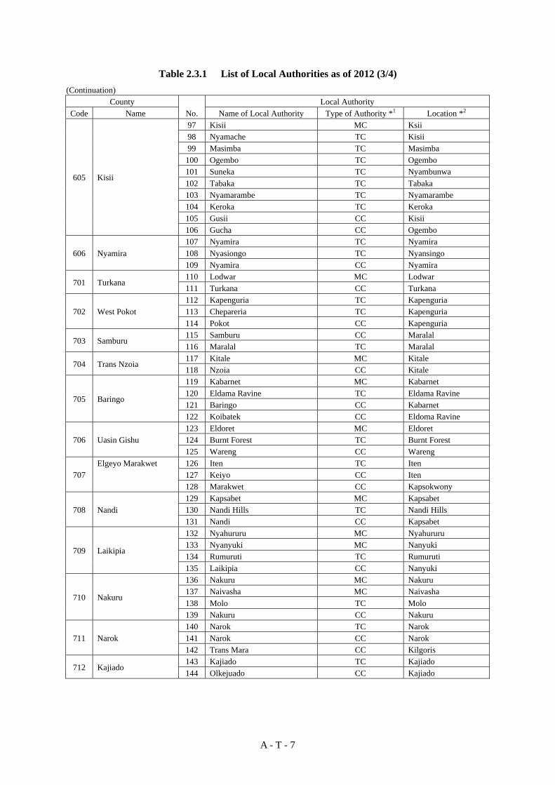
A - T - 7
Table 2.3.1 List of Local Authorities as of 2012 (3/4) (Continuation)
County No.
Local Authority Code Name Name of Local Authority Type of Authority *1 Location *2
605 Kisii
97 Kisii MC Ksii 98 Nyamache TC Kisii 99 Masimba TC Masimba 100 Ogembo TC Ogembo 101 Suneka TC Nyambunwa 102 Tabaka TC Tabaka 103 Nyamarambe TC Nyamarambe 104 Keroka TC Keroka 105 Gusii CC Kisii 106 Gucha CC Ogembo
606 Nyamira 107 Nyamira TC Nyamira 108 Nyasiongo TC Nyansingo 109 Nyamira CC Nyamira
701 Turkana 110 Lodwar MC Lodwar 111 Turkana CC Turkana
702 West Pokot 112 Kapenguria TC Kapenguria 113 Chepareria TC Kapenguria 114 Pokot CC Kapenguria
703 Samburu 115 Samburu CC Maralal 116 Maralal TC Maralal
704 Trans Nzoia 117 Kitale MC Kitale 118 Nzoia CC Kitale
705 Baringo
119 Kabarnet MC Kabarnet 120 Eldama Ravine TC Eldama Ravine 121 Baringo CC Kabarnet 122 Koibatek CC Eldoma Ravine
706 Uasin Gishu 123 Eldoret MC Eldoret 124 Burnt Forest TC Burnt Forest 125 Wareng CC Wareng
707 Elgeyo Marakwet 126 Iten TC Iten
127 Keiyo CC Iten 128 Marakwet CC Kapsokwony
708 Nandi 129 Kapsabet MC Kapsabet 130 Nandi Hills TC Nandi Hills 131 Nandi CC Kapsabet
709 Laikipia
132 Nyahururu MC Nyahururu 133 Nyanyuki MC Nanyuki 134 Rumuruti TC Rumuruti 135 Laikipia CC Nanyuki
710 Nakuru
136 Nakuru MC Nakuru 137 Naivasha MC Naivasha 138 Molo TC Molo 139 Nakuru CC Nakuru
711 Narok 140 Narok TC Narok 141 Narok CC Narok 142 Trans Mara CC Kilgoris
712 Kajiado 143 Kajiado TC Kajiado 144 Olkejuado CC Kajiado

A - T - 8
Table 2.3.1 List of Local Authorities as of 2012 (4/4) (Continuation)
County No.
Local Authority Code Name Name of Local Authority Type of Authority *1 Location *2
713 Kericho
145 Kericho MC Kericho 146 Londiani TC Londiani 147 Litein TC Litein 148 Kipkelion TC Kipkelion 149 Bureti CC Litein 150 Kipsigis CC Kericho
714 Bomet 151 Bomet MC Bomet 152 Sotik TC Sotik 153 Bomet CC Bomet
801 Kakamega
154 Kakamega MC Kakamega 155 Mumias MC Mumius 156 Malava TC Malava 157 Kakamega CC Kakamega 158 Butere-Mumias CC Butere 159 Lugari CC Lumakanda
802 Vihiga 160 Vihiga MC Mbale 161 Luanda TC Luanda 162 Vihiga CC Mbale
803 Bungoma
163 Bungoma MC Bungoma 164 Webuyu MC Webuye 165 Kimilili MC Kimilili 166 Sirisia TC Sirisia 167 Malakisi TC Malakisi 168 Mt.Elgon CC Kapisakwony 169 Bungoma CC Bungoma
804 Busia
170 Busia MC Busia 171 Funyula TC Funyula 172 Nambale TC Nambale 173 Port Victoria TC Port Victoria 174 Malaba TC Kamurai 175 Teso CC Amagoro 176 Busia CC Busia
Note: *1 The following shows the abbreviation used in the above: CITY: City Council MC: Municipal Council TC: Town Council CC: County Council
*2 “Location” points out a location where the Council is located. Source: Ministry of Local Government

A - T - 9
Table 2.3.2 Inventory of Local Authorities by Type and By County as of 2012 Code County Name City Council Municipal Council Town Council County Council 110 Nairobi City 1 - - - 201 Nyandarua - - 1 1 202 Nyeri - 2 1 1 203 Kirinyaga - 1 1 1 204 Murang’a - 1 4 2 205 Kiambu - 4 2 2 301 Mombasa 1 - - - 302 Kwale - - 1 1 303 Kilifi - 1 2 2 304 Tana River - - - 1 305 Lamu - - - 1 306 Taita/Taveta - 1 1 1 401 Marsabit - - - 2 402 Isiolo - - - 1 403 Meru - 2 - 2 404 Tharaka-Nithi - 1 1 2 405 Embu - 1 1 2 406 Kitui - 1 1 2 407 Machakos - 2 2 1 408 Makueni - - 2 1 501 Garissa - 1 - 2 502 Wajir - - - 1 503 Mandera - - 1 1 601 Siaya - 1 4 2 602 Kisumu 1 - 2 3 603 Migori - 2 2 1 604 Homa Bay - 1 3 3 605 Kisii - 1 7 2 606 Nyamira - - 2 1 701 Turkana - 1 - 1 702 West Pokot - - 2 1 703 Samburu - - 1 1 704 Trans Nzoia - 1 - 1 705 Baringo - 1 1 2 706 Uasin Gishu - 1 1 1 707 Elgeyo- Marakwet - - 1 2 708 Nandi - 1 1 1 709 Laikipia - 2 1 1 710 Nakuru - 2 1 1 711 Narok - - 1 2 712 Kajiado - - 1 1 713 Kericho - 1 3 2 714 Bomet - 1 1 1 801 Kakamega - 2 1 3 802 Vihiga - 1 1 1 803 Bungoma - 3 2 2 804 Busia - 1 4 2
Kenya 3 41 64 68 Source: Ministry of Local Government

A - T - 10
Table 3.1.1 Population Change, Household Size, and Density in 2009 (1/3)
County Previous Districts in
2009 Census Area (km2)
1999 Census 2009 Census
Code Name Population Population No. of Household
Family Size
Density (/km2)
110 Nairobi City Nairobi West, Nairobi East, Nairobi North, Westlands
696 2,143,254 3,138,369 985,016 3.19 4,509
201 Nyandarua Nyandarua North, Nyandarua South
3,248 479,902 596,268 143,879 4.14 184
202 Nyeri Nyeri North, Nyeri South
3,363 661,156 693,558 201,703 3.44 206
203 Kirinyaga Kirinyaga 1,479 457,105 528,054 154,220 3.42 357 204 Murang’a Muranga North,
Muranga South, Thika East, Gatanga
1,968 736,273 969,151 262,931 3.69 492
205 Kiambu Kiambu East, Kikuyu, Kiambu West(Limuru), Lari, Githunguri, Thika West, Ruiru, Gatundu
3,162 1,389,723 1,623,282 462,009 3.51 513
301 Mombasa Mombasa,Kilindini 177 665,018 939,370 268,700 3.50 5,307 302 Kwale Kwale, Kinango,
Msambweni 8,301 496,133 649,931 122,047 5.33 78
303 Kilifi Kilifi, Kaloleni, Malindi
12,517 825,855 1,109,735 199,764 5.56 89
304 Tana River Tana River, Tana Delta
38,376 180,901 240,075 47,414 5.06 6
305 Lamu Lamu 5,937 72,686 101,539 22,184 4.58 17 306 Taita/Taveta Taita, Taveta 17,330 246,671 284,657 71,090 4.00 16 401 Marsabit Marsabit, Chalbi,
Laisamis, Moyale 66,502 174,957 291,166 56,941 5.11 4
402 Isiolo Isiolo,Garbatula 25,201 100,861 143,294 31,326 4.57 6 403 Meru Meru Central,Imenti
North,Imenti South,Igembe, Tigania
6,952 1,102,930 1,356,301 319,616 4.24 195
404 Tharaka- Nithi
Meru South,Maara, Tharaka
2,651 306,443 365,330 88,803 4.11 138
405 Embu Embu, Mbeere 2,830 449,149 516,212 131,683 3.92 182 406 Kitui Kitui, Mutomo,
Mwingi, Kyuso 30,558 819,250 1,012,709 205,491 4.93 33
407 Machakos Machakos, Mwala, Yatta, Kangundo
6,242 906,644 1,098,584 264,500 4.15 176
408 Makueni Makueni, Mbooni, Kibwezi, Nzaui,
8,058 771,545 884,527 186,478 4.74 110
501 Garissa Garissa, Lagdera, Fafi, Ijara
44,071 392,510 623,060 98,590 6.32 14
502 Wajir Wajir South,Wajir North,Wajir East,Wajir West
56,184 319,261 661,941 88,574 7.47 12
503 Mandera Mandera Central, Mandera East, Mandera West
25,551 250,372 1,025,756 125,497 8.17 40

A - T - 11
Table 3.1.1 Population Change, Household Size, and Density in 2009 (2/3) (Continuation)
County Previous District in
2009 Census Area (km2)
1999 Census
2009 Census
Code Name Population PopulationNo. of
Household Family
Size Density (/km2)
601 Siaya Siaya, Bondo, Rarieda
1,540 718,964 842,304 199,034 4.23 547
602 Kisumu Kisumu East, Kisumu West, Nyando
1,539 804,289 968,909 226,719 4.27 630
603 Migori Migori, Rongo, Kuria West, Kuria East
2,646 666,784 917,170 180,211 5.09 347
604 Homa Bay Homa Bay, Suba, Rachuonyo
1,134 751,332 963,794 206,255 4.67 850
605 Kisii Kisii Central, Kisii South, Gucha, Gucha South
1,474 952,725 1,030,212 218,897 4.71 699
606 Nyamira Nyamira, Masaba, Manga, Borabu
758 498,102 720,322 157,171 4.58 950
701 Turkana Turkana Central, Turkana North, Turkana South
66,276 450,860 855,399 123,191 6.94 13
702 West Pokot West Pokot, Pokot Central, Pokot North
9,115 308,086 512,690 93,777 5.47 56
703 Samburu Samburu Central, Samburu East, Samburu North
21,014 143,547 223,947 47,354 4.73 11
704 Trans Nzoia Trans Nzoia East, Trans Nzoia West, Kwanza
2,509 575,662 818,757 170,117 4.81 326
705 Baringo Baringo Central, Baringo North, East Pokot, Koibatek
10,880 403,141 555,561 110,649 5.02 51
706 Uasin Gishu Eldoret West, Eldoret East, Wareng
3,364 622,705 894,179 202,291 4.42 266
707 Elgeyo/Marakwet
Marakwet, Keiyo 3,031 284,494 369,998 77,555 4.77 122
708 Nandi Nandi North, Nandi Central, Nandi East, Nandi South, Tinderet
2,904 578,751 752,965 154,073 4.89 259
709 Laikipia Laikipia North, Laikipia East, Laikipia West
9,514 322,187 399,227 103,114 3.87 42
710 Nakuru Nakuru, Naivasha, Molo, Nakuru North
7,410 1,187,039 1,603,325 409,836 3.91 216
711 Narok Narok North, Narok South, Trans Mara
18,278 536,341 850,920 169,220 5.03 47
712 Kajiado Kajiado Central, Kajiado North, Loitoktok
22,130 406,054 687,312 173,464 3.96 31
713 Kericho Kericho, Kipkellion 2,176 785,375 590,690 127,581 4.63 271

A - T - 12
Table 3.1.1 Population Change, Household Size, and Density in 2009 (3/3) (Continuation)
County Previous Districts in
2009 Census Area (km2)
1999 Census
2009 Census
Code Name Population PopulationNo. of
Household Family
Size Density (/km2)
714 Bomet Bomet, Sotik, Buret 2,831 382,794 891,835 174,914 5.10 315 801 Kakamega Kakamega Central,
Kakamega South, Kakamega North, Kakamega East, Lugari, Mumias, Butere
2,707 1,296,270 1,660,651 355,679 4.67 613
802 Vihiga Vihiga, Emuhaya, Hamisi
889 498,883 554,622 123,347 4.50 624
803 Bungoma Bungoma South, Bungoma North, Bungoma East, Bungoma West, Mt.Elgon
3,019 1,011,524 1,375,063 270,824 5.08 455
804 Busia Busia, Teso North, Samia, Bunyala, Teso South
1,552 552,099 743,946 154,225 4.82 479
Kenya 570,044 28,686,607 38,636,667 8,767,954 4.41 68 Source: 1999 Population and Housing Census; 2009 Population and Housing Census 2009, Kenya National Bureau of
Statistics

A - T - 13
Table 3.1.2 Population Distribution by Catchment Area and by County in 2009
Province County Population 2009
Population of County by Catchment Area in 2009 LVNCA LVSCA RVCA ACA TCA ENNCA
Western
Bungoma 1,375,063 1,375,063 0 0 0 0 0 Busia 743,946 743,946 0 0 0 0 0 Kakamega 1,660,651 1,660,651 0 0 0 0 0 Vihiga 554,622 471,429 83,193 0 0 0 0
Nyanza
Homa Bay 963,794 0 963,794 0 0 0 0 Migori 917,170 0 917,170 0 0 0 0 Kisii 1,030,212 0 1,030,212 0 0 0 0 Nyamira 720,322 0 720,322 0 0 0 0 Kisumu 968,909 465,076 503,833 0 0 0 0 Siaya 842,304 783,343 58,961 0 0 0 0
Rift Valley
Baringo 555,561 0 0 555,561 0 0 0 Kericho 590,690 448,924 141,766 0 0 0 0 Bomet 891,835 0 891,835 0 0 0 0 Elgeyo Marakwet
369,998 133,199 0 236,799 0 0 0
Kajiado 687,312 0 0 247,432 439,880 0 0 Laikipia 399,227 0 0 39,923 0 0 359,304 Nakuru 1,603,325 0 256,532 1,346,793 0 0 0 Nandi 752,965 685,198 67,767 0 0 0 0 Narok 850,920 0 459,497 391,423 0 0 0 Samburu 223,947 0 0 49,268 0 0 174,679 Trans Nzoia 818,757 753,256 0 65,501 0 0 0 Turkana 855,399 0 0 855,399 0 0 0 Uasin Gishu 894,179 894,179 0 0 0 0 0 West Pokot 512,690 0 0 512,690 0 0 0
Central Kiambu 1,623,282 0 0 129,863 1,006,435 486,985 0 Kirinyaga 528,054 0 0 0 0 528,054 0 Muranga 969,151 0 0 0 0 969,151 0 Nyandarua 596,268 0 0 333,910 0 35,776 226,582 Nyeri 693,558 0 0 0 0 478,555 215,003
Nairobi Nairobi 3,138,369 0 0 0 3,138,369 0 0 Eastern Embu 516,212 0 0 0 0 516,212 0
Isiolo 143,294 0 0 0 0 14,329 128,965 Kitui 1,012,709 0 0 0 50,635 962,074 0 Machakos 1,098,584 0 0 0 725,065 373,519 0 Makueni 884,527 0 0 0 884,527 0 0 Marsabit 291,166 0 0 43,675 0 0 247,491 Meru 1,356,301 0 0 0 0 705,277 651,024 Tharaka-Nithi
365,330 0 0 0 0 365,330 0
Coast Kilifi 1,012,709 0 0 0 860,803 151,906 0 Kwale 649,931 0 0 0 649,931 0 0 Lamu 101,539 0 0 0 0 101,539 0 Mombasa 939,370 0 0 0 939,370 0 0 Taita Taveta 284,657 0 0 0 284,657 0 0 Tana River 240,075 0 0 0 0 240,075 0
North Eastern
Garissa 623,060 0 0 0 0 417,450 205,610 Mandera 1,025,756 0 0 0 0 0 1,025,756 Wajir 661,941 0 0 0 0 0 661,941
Total 38,539,641 8,414,265 6,094,882 4,808,236 8,979,672 6,346,231 3,896,355
Source: 2009 Population and Housing Census, Kenya National Bureau of Statistics; JICA Study Team.

A - T - 14
Table 3.1.3 1999 Census and 2009 Census Population by County in Urban and Rural Areas County 1999 Census Population 2009 Census Population
Code Name Total Urban Rural Total Urban Rural Kenya 28,686,607 9,904,044 18,782,563 38,636,667 12,487,375 26,122,722
110 Nairobi City 2,143,254 2,143,254 - 3,138,369 3,138,369 - 201 Nyandarua 479,902 68,606 411,296 596,268 110,518 485,750 202 Nyeri 661,156 255,971 405,185 693,558 169,617 523,941 203 Kirinyaga 457,105 54,756 402,349 528,054 83,404 444,650 204 Murang’a 736,273 159,292 576,981 969,151 148,672 820,479 205 Kiambu * 1,389,723 584,197 805,526 1,623,282 1,014,006 582,706 301 Mombasa 665,018 665,018 - 939,370 939,370 - 302 Kwale 496,133 75,361 420,772 649,931 117,676 532,255 303 Kilifi 825,855 291,915 533,940 1,109,735 285,482 824,253 304 Tana River 180,901 15,430 165,471 240,075 36,065 204,010 305 Lamu 72,686 11,831 60,855 101,539 20,238 81,301 306 Taita/Taveta 246,671 101,200 145,471 284,657 64,289 220,368 401 Marsabit 174,957 41,798 133,159 291,166 64,009 227,157 402 Isiolo 100,861 40,252 60,609 143,294 62,374 80,920 403 Meru 1,102,930 155,492 947,438 1,356,301 115,033 1,241,268 404 Tharaka-Nithi 306,443 7,271 299,172 365,330 83,999 281,331 405 Embu 449,149 113,899 335,250 516,212 82,921 433,291 406 Kitui 819,250 172,985 646,265 1,012,709 139,909 872,800 407 Machakos 906,644 394,590 512,054 1,098,584 571,355 527,229 408 Makueni 771,545 130,091 641,454 884,527 104,297 780,230 501 Garissa 392,510 80,391 312,119 623,060 146,668 476,392 502 Wajir 319,261 54,378 264,883 661,941 96,855 565,086 503 Mandera 250,372 65,412 184,960 1,025,756 185,568 840,188 601 Siaya 718,964 145,759 573,205 842,304 90,627 751,677 602 Kisumu 804,289 397,802 406,487 968,909 507,720 461,189 603 Migori 666,784 421,220 245,564 917,170 311,512 605,658 604 Homa Bay 751,332 190,562 560,770 963,794 138,051 825,743 605 Kisii 952,725 295,078 657,647 1,030,212 181,359 848,853 606 Nyamira 498,102 132,387 365,715 720,322 158,663 561,659 701 Turkana 450,860 59,882 390,978 855,399 121,719 733,680 702 West Pokot 308,086 67,200 240,886 512,690 42,696 469,994 703 Samburu 143,547 36,763 106,784 223,947 38,664 185,283 704 Trans Nzoia 575,662 86,282 489,380 818,757 167,420 651,337 705 Baringo 403,141 62,313 340,828 555,561 61,551 494,010 706 Uasin Gishu 622,705 266,412 356,293 894,179 345,559 548,620 707 Elgeyo/Marakwet 284,494 22,710 261,784 369,998 53,186 316,812 708 Nandi 578,751 126,243 452,508 752,965 102,281 650,684 709 Laikipia 322,187 113,668 208,519 399,227 99,117 300,110 710 Nakuru 1,187,039 555,543 631,496 1,603,325 735,025 868,300 711 Narok 536,341 46,213 490,128 850,920 58,494 792,426 712 Kajiado 406,054 87,422 318,632 687,312 284,862 402,450 713 Kericho 785,375 154,183 631,192 590,690 228,318 362,372 714 Bomet 382,794 94,999 287,795 891,835 132,255 759,580 801 Kakamega 1,296,270 227,755 1,068,515 1,660,651 252,611 1,408,040 802 Vihiga 498,883 175,797 323,086 554,622 174,105 380,517 803 Bungoma 1,011,524 267,719 743,805 1,375,063 298,696 1,076,367 804 Busia 552,099 186,742 365,357 743,946 122,190 621,756
Note: * In Kiambu, the total population in 2009 does not match the total figure of urban and rural population.
Source: 1999 and 2009 Kenya Population and Housing Census, Kenya National Bureau of Statistics

A - T - 15
Table 3.1.4 Population in Urban Centres in 2009 (1/6)
No. M/P(*) Urban Centre Previous Districts
in 2009 Status Male Female Total Urban & Peri-urban
1 ○
NAIROBI Nairobi East/West/ North/ Westlands
City 1,602,104 1,531,414 3,133,518 3,133,518
2 ○ MOMBASA Mombasa/
kilindini City 486,208 451,923 938,131 938,131
3 ○ KISUMU Kisumu East/
West/ Nyando City 204,234 205,694 409,928 388,311
4 ○ NAKURU Nakuru/ Nakuru
North Municipality 155,881 152,109 307,990 307,990
5 ○
ELDORET Eldoret East/West/ Wareng
Municipality 146,596 142,784 289,380 289,380
6 ○ KEHANCHA Kuria East/west Municipality 125,938 130,148 256,086 30,109 7 ○ RUIRU Ruiru Municipality 119,147 119,711 238,858 238,858 8 ○ MALINDI Malindi/ Kilifi Municipality 103,079 104,174 207,253 118,265 9 ○ NAIVASHA Naivasha Municipality 91,371 90,595 181,966 169,142
10 ○ KITUI Kitui Municipality 75,741 80,155 155,896 109,568 11 ○ MACHAKOS Machakos Municipality 74,294 75,747 150,041 150,041 12
○ THIKA Thika West/ Gatanga
Municipality 69,697 70,156 139,853 136,917
13 ○ MAVOKO Machakos Municipality 76,056 63,324 139,380 137,211 14
○ NYERI Nyeri North/ South
Municipality 62,648 62,709 125,357 119,353
15 ○ VIHIGA Vihiga Municipality 56,807 61,889 118,696 118,696 16 ○ MUMIAS Mumias Municipality 56,783 59,575 116,358 99,987 17 ○ BOMET Bomet/Sotik Municipality 55,090 55,873 110,963 83,729 18 ○ KITALE Trans Nzoia West Municipality 54,065 52,122 106,187 106,187 19 ○ LIMURU Kiambu West Municipality 52,111 52,171 104,282 79,711 20 ○ KERICHO Kericho/kipkelion Municipality 53,452 50,459 103,911 101,808 21 ○ KIMILILI Bungoma North Municipality 46,007 48,920 94,927 94,927 22
○ KAKAMEGA Kakamega Central
Municipality 46,068 45,700 91,768 91,768
23 ○ KAPSABET Nandi Central Municipality 45,420 45,610 91,030 86,803 24 ○ KIAMBU Kiambu East Municipality 43,524 45,345 88,869 84,155 25
○ KISII Kisii Central/ Kisii South
Municipality 41,948 41,512 83,460 81,801
26 ○ BUNGOMA Bungoma South Municipality 40,086 41,065 81,151 55,867 27
○ WEBUYE Bungoma East/ Lugari
Municipality 31,954 33,326 65,280 41,344
28 ○ BUSIA Busia/ Teso South Municipality 29,927 31,788 61,715 51,981 29 ○ RUNYENJES Embu Municipality 30,268 31,336 61,604 19,548 30 ○ MIGORI Migori Municipality 29,527 31,522 61,049 53,100 31 ○ EMBU Embu Municipality 29,768 30,905 60,673 60,673 32 ○ HOMA BAY Homa Bay Municipality 28,501 31,343 59,844 58,936 33 ○ LODWAR Turkana Central* Municipality 28,497 29,721 58,218 48,316 34 ○ MERU Imenti North Municipality 26,418 27,209 53,627 53,627 35
○ NYAHURURU
Laikipia West Municipality 25,183 26,251 51,434 36,450
36 ○ NANYUKI Laikipia East Municipality 25,046 24,187 49,233 38,198 37 ○ MAUA Igembe Municipality 24,027 24,985 49,012 17,226 38 ○ VOI Taita Municipality 23,611 21,872 45,483 17,152

A - T - 16
Table 3.1.4 Population in Urban Centres in 2009 (2/6) (Continuation)
No. M/P(*) Urban Centre
Previous Districts
Status Male Female Total Urban &
Peri-urban39 ○ SIAYA Siaya Municipality 21,575 23,778 45,353 22,586 40 ○ CHUKA Meru South Municipality 21,266 22,204 43,470 43,470 41
○ KERUGOYA/KUTUS
Kirinyaga Municipality 16,766 17,248 34,014 19,422
42 ○ MURANGA Muranga North Municipality 14,069 14,706 28,775 28,775 43 ○ KABARNET Baringo Central Municipality 12,813 14,465 27,278 25,346 44 ○ KARATINA Nyeri North Municipality 3,738 4,761 8,499 8,499 45 ○ NGONG Kajiado North Other center 54,040 53,148 107,188 107,188 46
○ AWASI Nyando/Kisumu East
Other center 44,934 48,435 93,369 93,369
47 ○ WAJIR Wajir East* Other center 43,684 39,116 82,800 82,800 48 ○ KAKUMA Turkana North* Other center 34,560 31,254 65,814 36,875 49 ○ UKUNDA Msambweni Other center 32,011 30,518 62,529 62,529 50 ○ WUNDANYI Taita Other center 31,400 31,004 62,404 62,404 51 ○ KITENGELA Kajiado North Other center 30,088 28,079 58,167 58,167 52 ○ MTWAPA Kilifi Other center 24,134 24,491 48,625 48,625 53
○ ISIOLO Isiolo/ Imenti North
Other center 22,827 23,301 46,128 45,989
54 ○ JUJA Thika West Other center 20,488 19,958 40,446 40,446 55
○ ONGATA RONGAI
Kajiado North Other center 19,271 20,907 40,178 40,178
56 ○ MOYALE Moyale Other center 18,916 18,471 37,387 37,387 57 ○ GILGIL Naivasha Other center 18,570 16,723 35,293 35,293 58
○ RHAMU Mandera Central*
Other center 18,142 12,909 31,051 26,367
59 ○ WANGURU Kirinyaga Other center 12,225 12,707 24,932 23,983 60
○ ELWAK Mandera Central*
Other center 13,125 11,243 24,368 24,368
61 ○ NJORO Molo Other center 11,332 12,219 23,551 23,551 62
○ MOI'S BRIDGE Lugari/ Eldoret West
Other center 10,698 11,467 22,165 14,596
63 ○ LOKICHOGIO Turkana North* Other center 11,583 10,573 22,156 17,695 64 ○ TAKABA Mandera West* Other center 11,835 9,639 21,474 21,474 65
○ AWENDO Homabay/Rongo
Other center 10,388 10,499 20,887 17,992
66 ○ LAMU Lamu Other center 9,977 9,488 19,465 18,382 67 ○ CHWELE Bungoma West Other center 9,119 10,044 19,163 7,206 68 ○ KISERIAN Kajiado North Other center 9,024 9,072 18,096 18,096 69 ○ HOLA Tana River Other center 8,470 8,867 17,337 17,337 70 ○ USENGE Bondo Other center 7,820 8,115 15,935 10,098 71 ○ MADOGO Tana River Other center 8,152 7,672 15,824 15,824 72 ○ MARSABIT Marsabit Other center 7,525 7,382 14,907 14,907 73 ○ MASALANI Ijara Other center 7,374 6,638 14,012 14,012 74 ○ BUTERE Butere Other center 5,998 6,782 12,780 12,780 75 ○ MSAMBWENI Msambweni Other center 5,819 6,166 11,985 11,985 76
○ KIMININI Trans Nzoia West
Other center 5,367 6,292 11,659 11,659
77 ○ MAI MAHIU Naivasha Other center 5,617 5,613 11,230 11,230 78 ○ LOITOKTOK Loitoktok Other center 5,617 5,447 11,064 11,064 79 ○ LUMAKANDA Lugari Other center 5,259 5,321 10,580 10,580

A - T - 17
Table 3.1.4 Population in Urban Centres in 2009 (3/6) (Continuation)
No. M/P(*) Urban Centre Previous Districts Status Male Female Total
Urban & Peri-urban
80 ○ MATUNDA Eldoret West/Lugari
Other center 4,756 5,275 10,031 10,031
81 ○ WATAMU Malindi Other center 5,167 4,863 10,030 10,030 82 ○ GITHUGURI Githunguri Other center 4,843 5,164 10,007 10,007 83 KILGORIS Trans Mara Other center 4,926 4,939 9,865 9,865 84 MAIRO_INY
A Nyandarua North Other center 4,792 5,066 9,858 9,858
85 WAMBA Samburu East Other center 4,817 4,805 9,622 6,226 86 NAMANGA Kajiado Central Other center 4,684 4,382 9,066 9,066 87 SORI Migori Other center 4,478 4,486 8,964 8,964 88 MAKINDU Kibwezi Other center 4,183 4,700 8,883 8,621 89 ISINYA Kajiado North Other center 4,765 3,905 8,670 8,670 90 HABASWEI
N Wajir South/ West Other center 4,594 3,906 8,500 8,500
91 TIMAU Imenti North Other center 4,177 4,156 8,333 8,333 92 BARAGOI Samburu North Other center 3,825 4,167 7,992 7,992 93 KINANGO Kinango Other center 3,895 4,063 7,958 7,958 94 CHEMELIL Nyando/Kisumu
East Other center 4,331 3,557 7,888 7,888
95 MAJENGO Kilifi Other center 3,892 3,896 7,788 7,788 96 NKUBU Imenti South Other center 3,770 3,781 7,551 7,551 97 SUBUKIA Nakuru North Other center 3,460 3,849 7,309 7,309 98 MARIGAT Barigo Other center 3,557 3,603 7,160 6,661 99 EMALI Nzaui Other center 3,494 3,530 7,024 7,024 100 MAZERAS Kaloleni Other center 3,259 3,627 6,886 6,886 101 SULTAN
HAMUD Nzaui/Kajiado central
Other center 3,427 3,209 6,636 6,636
102 MERTI Isiolo Other center 3,103 3,429 6,532 6,532 103 KALOLENI Kaloleni Other center 3,202 3,236 6,438 5,573 104 SINDO Suba Other center 2,980 3,382 6,362 6,362 105 ARCHERS
POST Samburu Other center 3,226 3,049 6,275 6,275
106 MUHURU BAY
Migori Other center 3,016 3,238 6,254 6,254
107 KAPSOKWONY
Mt.Elgon Other center 3,035 3,117 6,152 6,152
108 MAGARINI Malindi Other center 2,936 3,115 6,051 6,051 109 NJABINI Nyandarua South Other center 3,003 3,039 6,042 6,042 110 MARERENI Malindi Other center 2,869 3,080 5,949 5,949 111 NAIRAGIE
ENKARE Narok North Other center 2,915 2,992 5,907 5,907
112 KIBWEZI Kibwezi Other center 2,892 2,979 5,871 5,871 113 NARO
MORU Nyeri North/Laikipia East
Other center 2,965 2,840 5,805 5,805
114 DADAAB Lagdera Other center 3,075 2,648 5,723 5,723 115 MWATATE Taita Other center 2,761 2,812 5,573 5,573 116 GATUNDU Gatundu Other center 2,580 2,970 5,550 5,550 117 BISSIL Kajiado Central Other center 2,509 2,867 5,376 5,376 118 DUNDORI Nakuru North Other center 2,528 2,693 5,221 5,221

A - T - 18
Table 3.1.4 Population in Urban Centres in 2009 (4/6) (Continuation)
No. M/P(*) Urban Centre Previous District Status Male Female Total
Urban & Peri-urban
119 LOIYANGALANI
Laisamis Other center 2,272 2,845 5,117 4,208
120 SOLOLO Moyale Other center 2,543 2,561 5,104 5,104 121 MASENO Kisumu West Other center 2,506 5,103 5,103 5,103 122 KINNA Garbatulla Other center 2,427 2,440 4,867 4,867 123 SALGAA Nakuru Other center 2,390 2,350 4,740 4,740 124 LARE Igembe Other center 2,350 2,264 4,614 4,614 125 KAPSOWAR Marakwet Other center 2,189 2,303 4,492 4,492 126 MAU
NAROK Molo Other center 2,112 2,245 4,357 4,357
127 MAJI MAZURI
Koibatek Other center 2,193 2,072 4,265 4,265
128 KABUTI Kericho Other center 2,144 2,093 4,237 4,237 129 CHEPTAIS Mt.Elgon Other center 1,852 2,047 3,899 3,899 130 BAHATI Nakuru North Other center 1,806 2,027 3,833 3,833 131 GARBATUL
A Garbatulla Other center 1,931 1,843 3,774 3,774
132 KIRIA_INI Muranga North Other center 1,733 1,978 3,711 2,457 133 MOGOTIO Koibatek Other center 1,808 1,893 3,701 3,701 134 LUNGA
LUNGA Msambweni Other center 1,847 1,823 3,670 3,670
135 MWEIGA Nyeri North Other center 1,698 1,885 3,583 3,583 136 BUMALA Busia Other center 1,611 1,893 3,504 3,504 137 KAGUMO Kirinyaga Other center 1,585 1,864 3,449 3,449 138 JUA KALI Eldoret West Other center 1,633 1,794 3,427 3,427 139 MATUNGUU Imenti South Other center 1,690 1,712 3,402 3,402 140 KATHIANI Machakos Other center 1,598 1,767 3,365 3,365 141 KAGIO Kirinyaga Other center 1,548 1,809 3,357 3,357 142 KAPCHERO
P Marakwet Other center 1,559 1,609 3,168 3,168
143 TIMBOROA Koibatek Other center 1,551 1,599 3,150 3,150 144 KABATI Muranga Other center 1,529 1,599 3,128 3,128 145 ENDARASH
A Nyeri North Other center 1,429 1,620 3,049 3,049
146 GARSEN Tana Delta Other center 1,484 1,420 2,904 2,904 147 TURBO Eldoret West Other center 1,419 1,412 2,831 2,831 148 KANGARI Muranga South Other center 1,395 1,415 2,810 2,810 149 TONGAREN Bungoma North Other center 1,340 1,453 2,793 2,793 150 SIAKAGO Mbeere Other center 1,319 1,375 2,694 2,694 151 LOLGORIAN Trans Mara Other center 1,373 1,316 2,689 2,689 152 LAISAMIS Laisamis Other center 1,370 1,273 2,643 2,643 153 MOGONGA Gucha Other center 1,268 1,277 2,545 2,545 154 NDORI Rarieda Other center 1,223 1,299 2,522 2,522 155 MACHINER
Y Kibwezi Other center 1,310 1,195 2,505 2,505
156 MASII Mwala Other center 1,188 1,313 2,501 2,501 157 KINAMBA Laikipia West Other center 1,142 1,177 2,319 2,319 158 RONGAI Nakuru Other center 1,105 1,110 2,215 2,215
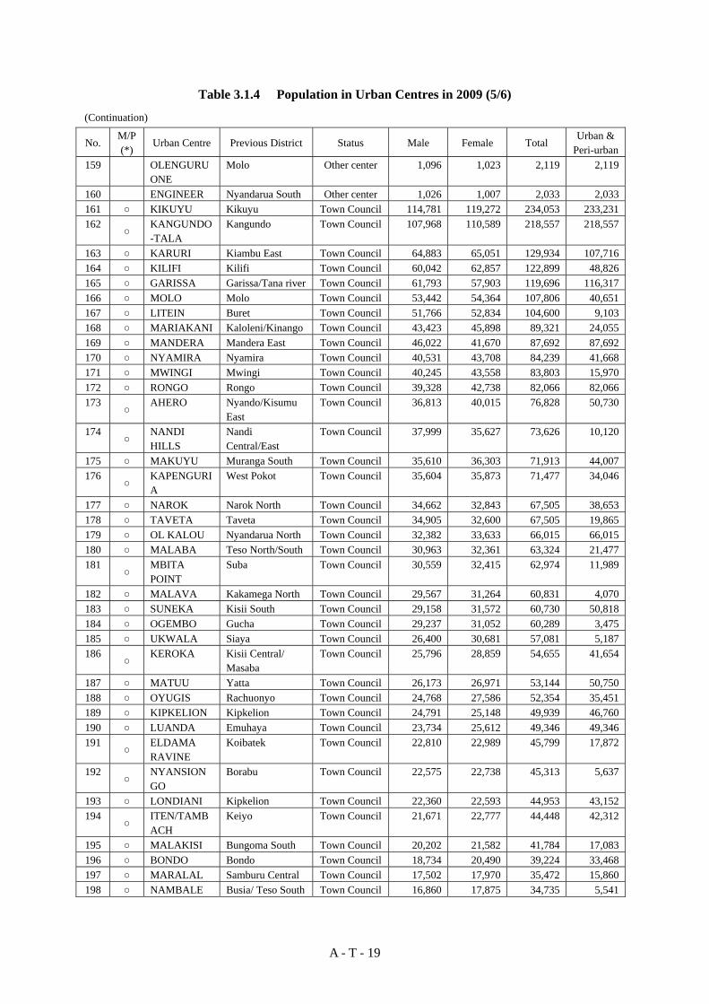
A - T - 19
Table 3.1.4 Population in Urban Centres in 2009 (5/6)
(Continuation)
No. M/P(*) Urban Centre Previous District Status Male Female Total
Urban & Peri-urban
159 OLENGURUONE
Molo Other center 1,096 1,023 2,119 2,119
160 ENGINEER Nyandarua South Other center 1,026 1,007 2,033 2,033 161 ○ KIKUYU Kikuyu Town Council 114,781 119,272 234,053 233,231 162
○ KANGUNDO-TALA
Kangundo Town Council 107,968 110,589 218,557 218,557
163 ○ KARURI Kiambu East Town Council 64,883 65,051 129,934 107,716 164 ○ KILIFI Kilifi Town Council 60,042 62,857 122,899 48,826 165 ○ GARISSA Garissa/Tana river Town Council 61,793 57,903 119,696 116,317 166 ○ MOLO Molo Town Council 53,442 54,364 107,806 40,651 167 ○ LITEIN Buret Town Council 51,766 52,834 104,600 9,103 168 ○ MARIAKANI Kaloleni/Kinango Town Council 43,423 45,898 89,321 24,055 169 ○ MANDERA Mandera East Town Council 46,022 41,670 87,692 87,692 170 ○ NYAMIRA Nyamira Town Council 40,531 43,708 84,239 41,668 171 ○ MWINGI Mwingi Town Council 40,245 43,558 83,803 15,970 172 ○ RONGO Rongo Town Council 39,328 42,738 82,066 82,066 173
○ AHERO Nyando/Kisumu East
Town Council 36,813 40,015 76,828 50,730
174 ○ NANDI
HILLS Nandi Central/East
Town Council 37,999 35,627 73,626 10,120
175 ○ MAKUYU Muranga South Town Council 35,610 36,303 71,913 44,007 176
○ KAPENGURIA
West Pokot Town Council 35,604 35,873 71,477 34,046
177 ○ NAROK Narok North Town Council 34,662 32,843 67,505 38,653 178 ○ TAVETA Taveta Town Council 34,905 32,600 67,505 19,865 179 ○ OL KALOU Nyandarua North Town Council 32,382 33,633 66,015 66,015 180 ○ MALABA Teso North/South Town Council 30,963 32,361 63,324 21,477 181
○ MBITA POINT
Suba Town Council 30,559 32,415 62,974 11,989
182 ○ MALAVA Kakamega North Town Council 29,567 31,264 60,831 4,070 183 ○ SUNEKA Kisii South Town Council 29,158 31,572 60,730 50,818 184 ○ OGEMBO Gucha Town Council 29,237 31,052 60,289 3,475 185 ○ UKWALA Siaya Town Council 26,400 30,681 57,081 5,187 186
○ KEROKA Kisii Central/ Masaba
Town Council 25,796 28,859 54,655 41,654
187 ○ MATUU Yatta Town Council 26,173 26,971 53,144 50,750 188 ○ OYUGIS Rachuonyo Town Council 24,768 27,586 52,354 35,451 189 ○ KIPKELION Kipkelion Town Council 24,791 25,148 49,939 46,760 190 ○ LUANDA Emuhaya Town Council 23,734 25,612 49,346 49,346 191
○ ELDAMA RAVINE
Koibatek Town Council 22,810 22,989 45,799 17,872
192 ○ NYANSION
GO Borabu Town Council 22,575 22,738 45,313 5,637
193 ○ LONDIANI Kipkelion Town Council 22,360 22,593 44,953 43,152 194
○ ITEN/TAMBACH
Keiyo Town Council 21,671 22,777 44,448 42,312
195 ○ MALAKISI Bungoma South Town Council 20,202 21,582 41,784 17,083 196 ○ BONDO Bondo Town Council 18,734 20,490 39,224 33,468 197 ○ MARALAL Samburu Central Town Council 17,502 17,970 35,472 15,860 198 ○ NAMBALE Busia/ Teso South Town Council 16,860 17,875 34,735 5,541

A - T - 20
Table 3.1.4 Population in Urban Centres in 2009 (6/6) (Continuation)
No. M/P(*) Urban Centre Previous Districts Status Male Female Total
Urban & Peri-urban
199 ○ TABAKA Gucha South Town Council 16,781 17,943 34,724 15,351 200
○ MUHORONI Nyando/Kisumu East
Town Council 17,892 16,565 34,457 34,457
201 ○ UGUNJA Siaya Town Council 15,760 18,118 33,878 7,242 202 ○ YALA Siaya Town Council 15,992 17,654 33,646 6,412 203 ○ RUMURUTI Laikipia West Town Council 15,956 17,037 32,993 10,064 204
○ BURNT FOREST
Eldoret East/ Wareng
Town Council 16,364 16,285 32,649 4,925
205 ○ MARAGUA Muranga South Town Council 15,772 16,543 32,315 26,374 206 ○ KENDU BAY Rachuonyo Town Council 15,279 16,420 31,699 15,103 207 ○ CHOGORIA Maara Town Council 15,850 15,773 31,623 28,415 208 ○ KWALE Kwale Town Council 13,671 14,581 28,252 19,880 209 ○ SAGANA Kirinyaga Town Council 13,274 13,873 27,147 10,195 210
○ MTITO ANDEI
Kibwezi Town Council 13,086 12,833 25,919 4,520
211 ○ SOTIK Sotik Town Council 11,234 10,763 21,997 8,366 212
○ PORT VICTORIA
Bunyula Town Council 10,438 11,263 21,701 6,561
213 ○ OTHAYA Nyeri south Town Council 8,974 9,969 18,943 5,137 214 ○ KAJIADO Kajiado Central Town Council 9,283 8,998 18,281 14,860 215 ○ WOTE Makueni Town Council 4,887 4,988 9,875 9,875
Total 6,882,529 6,842,046 13,722,069 11,546,351
Note: * ○:Urban Centres subject to urban water supply development in the NWMP 2030.
Source: 2009 Population and Housing Census.

A - T - 21
Table 3.2.1 Projected Population Distribution by County and Catchment Area in 2030 Old Administration 1992
County Population Projection, 2030 (thousand)
Province District LVNCA LVSCA RVCA ACA TCA ENNCA Total Western Bungoma Bungoma 2,383 0 3 0 0 0 2,385
Busia Busia 791 0 0 0 0 0 791 Kakamega Kakamega 2,183 0 0 0 0 0 2,183 Vihiga 1,101 92 0 0 0 0 1,193
Nyanza South Nyanza Homa Bay 0 1,382 0 0 0 0 1,382 Migori 0 2,053 0 0 0 0 2,053 Kisii Kisii 0 2,420 0 0 0 0 2,420 Nyamira 0 452 0 0 0 0 452 Kisumu Kisumu 34 2,443 0 0 0 0 2,476 Siaya Siaya 848 187 0 0 0 0 1,035
Rift Valley
Baringo Baringo 0 1 622 0 0 0 623 Kericho Kericho 0 1,444 1 0 0 0 1,446 Bomet 0 1,295 0 0 0 0 1,295 Elgeyo Marakwet
Elgeyo Marakwet
310 0 220 0 0 0 530
Kajiado Kajiado 0 0 148 1,270 0 0 1,417 Laikipia Laikipia 0 0 38 0 3 707 747 Nakuru Nakuru 0 278 3,727 0 0 1 4,006 Nandi Nandi 857 200 0 0 0 0 1,057 Narok Narok 0 459 494 0 0 0 953 Samburu Samburu 0 0 62 0 0 223 285 Trans Nzoia Trans Nzoia 1,813 0 68 0 0 0 1,882 Turkana Turkana 0 0 831 0 0 0 831 Uasin Gishu Uasin Gishu 1,858 15 13 0 0 0 1,885 West Pokot West Pokot 183 0 423 0 0 0 606
Central Kiambu Kiambu 0 0 78 3,716 681 0 4,475 Kirinyaga Kirinyaga 0 0 0 0 785 1 786 Muranga Muranga 0 0 3 0 1,344 0 1,347 Nyandarua Nyandarua 0 0 695 3 48 208 954 Nyeri Nyeri 0 0 0 0 1,163 122 1,285
Nairobi Nairobi Nairobi 0 0 0 6,085 0 0 6,085 Eastern Embu Embu 0 0 0 0 779 0 779
Isiolo Isiolo 0 0 0 0 19 360 379 Kitui Kitui 0 0 0 22 1,408 0 1,431 Machakos Machakos 0 0 0 2,428 430 0 2,858 Makueni 0 0 0 1,161 0 0 1,161 Marsabit Marsabit 0 0 21 0 0 297 317 Meru Meru 0 0 0 0 1,255 572 1,827 Tharaka-Nithi 0 0 0 0 437 0 437
Coast Kilifi Kilifi 0 0 0 1,730 70 0 1,799 Kwale Kwale 0 0 0 920 0 0 920 Lamu Lamu 0 0 0 0 1,318 0 1,318 Mombasa Mombasa 0 0 0 2,651 0 0 2,651 Taita Taveta Taita Taveta 0 0 0 555 0 0 555 Tana River Tana River 0 0 0 2 235 0 237
North Eastern
Garissa Garissa 0 0 0 0 394 241 635 Mandera Mandera 0 0 0 0 0 1,021 1,021 Wajir Wajir 0 0 0 0 0 642 642
Total 12,361 12,719 7,446 20,543 10,369 4,395 67,833 Source: JICA Study Team based on GIS data from Kenya National Bureau of Statistics and Population Projection in the study

A - T - 22
Table 4.1.1 Gross Domestic Product by Activity/Industry between 2007 and 2011 (Unit: KSh million, constant price)
Industry 2007 2008 2009 2010 2011 Agriculture And Forestry 397,057 470,753 555,288 545,927 726,160
Growing of Crops and Horticulture 289,595 345,841 399,474 405,265 546,616 Farming of Animals 82,868 99,697 127,704 109,535 144,804
Agricultural and Animal Husbandry Services
8,573 8,764 9,571 10,934 12,580
Forestry and Logging 16,021 16,452 18,539 20,193 22,159 Fishing 7,127 9,450 9,903 14,637 15,091 Mining and Quarrying 12,904 14,930 12,083 17,650 20,621 Manufacturing 190,497 228,304 234,556 252,122 285,698
Manufacturing of Food, Beverages and Tobacco
57,865 65,123 75,615 79,162 97,053
All Other Manufacturing 132,632 163,181 158,941 172,960 188,645 Electricity and Water Supply 26,633 43,767 44,185 35,592 26,071
Electricity Supply 14,728 31,136 28,866 17,929 5,463 Water Supply 11,904 12,631 15,318 17,663 20,608
Construction 69,556 80,407 97,445 109,146 125,046 Wholesale And Retail Trade 177,609 214,022 233,001 260,869 320,950 Hotels and Restaurants 29,612 23,745 39,421 42,546 50,557 Transport and Communication 194,093 216,052 234,752 253,958 292,601
Transport and Storage 139,128 159,296 172,244 189,426 227,373 Post and Telecommunications 54,964 56,756 62,508 64,532 65,228
Financial Intermediation 88,018 97,806 128,732 143,471 193,044 Real Estate, Renting and Business Services 96,273 107,323 116,657 123,173 134,746
Dwellings, Owner Occupied and Rented 49,120 53,338 58,291 61,598 65,098 Renting and Business Services 47,153 53,985 58,366 61,575 69,648
Public Administration and Defense 107,508 106,431 118,662 141,648 151,321 Education 123,498 132,229 142,235 158,738 176,537 Health and Social Work 45,318 51,591 60,196 65,170 74,979 Other Community, Social and Personal Services
63,207 71,586 79,423 84,415 96,423
Private Household With Employed Persons 7,176 8,207 10,171 11,217 13,227 Less: Financial Services Indirectly Measured -20,074 -18,231 -25,762 -21,652 -31,787 All Industries at Basic Prices 1,616,010 1,858,371 2,090,948 2,238,630 2,671,285 Taxes Less Subsidies on Products 217,501 249,218 276,036 311,195 353,497 GDP at Market Prices 1,833,511 2,107,589 2,366,984 2,549,825 3,024,782 Source: Economic Survey 2012

A - T - 23
Table 4.1.2 Wholesale Prices of Major Agricultural Commodities between 2006 and 2012 (Unit: KSh)
Commodity Unit (kg)
Annual Whole Prices, 2006- 2011 Growth 08/12
Average 08/12 2006 2007 2008 2009 2010 2011 2012*
Avocado 90 992 679 1,044 1,555 1,405 1,524 2,080 18.8% 1,522 Banana Cooking 22 304 958 365 395 386 473 646 15.3% 453 Banana Ripe 14 314 328 391 562 482 557 496 6.1% 498 Beans Canadian 90 3,700 3,045 4,911 5,077 4,781 5,716 5,500 2.9% 5,197 Beans Dolichos 90 4,472 3,131 5,251 6,857 8,358 6,561 6,825 6.8% 6,770 Beans Mwezi moja 90 2,573 4,691 5,382 4,465 5,010 4,650 -0.2% 4,840 Beans Mwitemania 90 3,194 2,716 5,088 5,347 4,351 5,425 5,250 0.8% 5,092 Beans Rose coco 90 3,357 3,109 5,052 5,217 4,629 5,661 5,630 2.7% 5,238 Brinjals 44 1,138 1,017 1,220 1,347 1,454 1,305 1,550 6.2% 1,375 Cabbages 99 1,347 1,178 1,269 1,971 1,528 1,618 1,600 6.0% 1,597 Capsicumus 50 1,214 1,478 1,606 2,120 2,169 2,391 2,280 9.2% 2,113 Carrots 138 1,916 1,529 2,464 3,522 2,583 3,067 1,800 -7.5% 2,687 Cassava Fresh 99 1,176 2,859 1,145 1,716 1,471 1,609 1,967 14.5% 1,582 Cauliflower 39 1,265 1,370 1,930 2,028 1,887 1,779 1,885 -0.6% 1,902 Chilies 38 987 1,301 1,257 2,010 1,505 1,952 2,685 20.9% 1,882 Cowpeas 90 4,228 3,351 4,523 6,231 5,263 5,662 6,190 8.2% 5,574 Cucumber 50 943 692 1,418 1,568 1,672 1,733 1,700 4.6% 1,618 Eggs Tray 161 279 223 232 323 400 304 8.1% 296 Finger Millet 90 2,870 2,107 3,890 4,693 4,462 4,927 6,274 12.7% 4,849 Fresh Peas 51 1,803 1,333 2,259 2,970 2,457 2,755 1,840 -5.0% 2,456 Green Grams 90 5,560 3,433 5,093 6,979 7,050 8,619 7,240 9.2% 6,996 Groundnut-shell 110 5,461 4,979 7,190 7,921 8,674 9,928 11,180 11.7% 8,979 Irish Potatoes 110 1,801 1,747 2,308 2,874 2,503 3,279 4,460 17.9% 3,085 Kales 50 978 598 676 1,116 799 773 860 6.2% 845 Lemons 95 760 829 1,009 967 1,110 1,953 1,450 9.5% 1,298 Lettuces 51 980 1,500 1,611 2,240 1,613 1,994 2,300 9.3% 1,952 Limes 13 619 1,228 1,094 869 891 581 930 -4.0% 873 Maize Dry 90 1,368 1,118 2,016 2,667 1,652 2,907 2,900 9.5% 2,428 Maize Green 115 2,018 1,514 2,110 2,644 2,237 2,466 2,610 5.5% 2,413 Mangos, local 126 1,036 901 1,013 1,141 1,183 1,424 2,480 25.1% 1,448 Mangos, Ngowe 126 766 1,538 710 899 848 807 1,413 18.8% 935 Onion, dry 13 409 780 583 738 736 621 848 9.8% 705 Onion, spring 142 1,097 1,669 1,770 1,931 1,773 2,131 1,380 -6.0% 1,797 Oranges 93 1,560 1,493 1,726 2,070 2,168 2,631 2,920 14.0% 2,303 Passion fruits 57 1,680 1,414 1,825 2,313 2,962 3,140 3,534 18.0% 2,755 Paw paw 54 718 1,017 923 1,031 983 1,201 1,724 16.9% 1,172 Pineapples 13 453 925 587 667 738 769 742 6.0% 701 Sorghum 90 1,899 1,544 2,257 3,275 2,590 3,064 3,750 13.5% 2,987 Sweet potatoes 98 1,522 1,371 1,909 2,428 1,904 2,668 2,900 11.0% 2,362 Tomatoes 64 1,453 1,797 1,796 2,133 2,486 2,752 4,040 22.5% 2,641 Wheat 90 1,009 4,113 3,656 3,477 4,055 2,900 -8.4% 3,640
Note: * indicates the wholesale price as of November 1, 2012
Source: Economic Review of Agriculture 2012, Ministry of Agriculture; Business Daily, November 2, 2012

A - T - 24
Table 6.1.1 Percentage Distribution of Household by Main Source of Drinking Water (1/2) (Unit: %)
County Previous District in
1992
Piped into
Dwelling
Piped into Plot
Public Tap
Borehole with
Pump
Tanker/ Truck/ Vendor
River/ Pond
OthersCode Name
KENYA 7.6 13.7 11.2 6.2 4.2 20.5 36.6 RURAL 3.8 8.0 7.0 7.7 2.2 26.4 44.9 URBAN 18.8 31.1 24.1 1.9 10.3 2.5 11.3
110 Nairobi City Nairobi 27.8 40.0 27.2 0.2 2.7 2.1 CENTRAL 7.5 21.6 2.8 4.2 3.5 25.1 35.3 201 Nyandarua Nyandarua 4.0 10.8 0.4 4.9 2.0 23.0 54.9 202 Nyeri Nyeri 8.3 29.5 8.5 0.9 1.6 19.6 31.6 203 Kirinyaga Kirinyaga 19.1 7.6 1.4 0.2 33.8 37.9 204 Murang’a Murang’a/ Muragua 4.2 10.6 2.2 0.5 1.9 45.5 35.2 205 Kiambu * Kiambu/Thika 4.6 31.4 3.1 15.6 7.5 20.5 17.3
COAST 8.5 7.7 35.8 3.8 19.9 6.7 17.6 301 Mombasa Mombasa 10.8 11.1 40.9 0.4 35.4 1.4 302 Kwale Kwale 2.9 2.5 44.5 12.1 4.3 1.8 31.9 303 Kilifi Kilifi/Malindi 13.5 3.9 37.1 21.2 9.2 15.2 304 Tana River Tana River 1.1 2.3 2.2 20.7 8.0 23.7 42.0 305 Lamu Lamu 11.4 2.3 2.8 32.1 9.3 51.4 306 Taita/Taveta Taita Taveta 4.6 19.2 27.4 0.5 23.0 25.3
EASTERN 3.5 13.4 11.8 5.3 1.5 28.1 36.4 401 Marsabit Marsabit/ Moyale 1.5 8.3 12.5 16.5 9.0 18.1 34.2 402 Isiolo Isiolo 20.4 17.5 0.6 11.8 49.7 403 Meru Meru Central/ Meru
North 9.0 48.5 12.9 0.2 15.0 14.4
404 Tharaka/ Nithi Tharaka/ Nithi 1.9 3.2 5.0 15.9 2.3 52.9 18.8 405 Embu Embu/ Mbeere 3.2 21.7 2.4 6.1 0.7 35.8 30.3 406 Kitui Kitui/Mwingi 0.9 0.2 9.7 1.8 1.0 58.6 27.9 407 Machakos Machakos 2.9 2.4 14.3 13.0 3.4 14.6 49.4 408 Makueni Makueni 4.6 12.6 5.1 0.8 22.1 54.8
NORTH EASTERN 0.1 5.0 1.2 18.8 12.1 15.0 47.8 501 Garissa Garissa 11.7 2.6 10.7 5.2 10.0 59.8 502 Wajir Wajir 0.1 31.6 13.2 7.6 47.5 503 Mandera Mandera 0.2 1.8 0.6 13.8 20.7 32.2 30.7
NYANZA 2.2 2.9 9.6 7.6 2.9 17.1 57.7 601 Siaya Siaya/ Bondo 1.8 3.6 19.9 7.8 1.6 31.3 34.2 602 Kisumu Kisumu/ Nyando 6.4 4.2 25.6 10.7 6.5 15.4 31.4 603 Migori Migori/ Kuria 0.3 0.4 2.1 9.4 4.1 17.8 66.1 604 Homa Bay Homa Bay/
Rachuonyo/ Suba 0.5 2.4 4.2 11.8 1.1 30.6 49.6
605 Kisii Kisii Central/ Gucha (S. Kisii)
0.9 4.4 1.2 1.9 1.4 3.8 86.5
606 Nyamira N. Kisii (Nyamira) 0.4 0.8 0.1 0.7 7.1 90.9 RIFT VALLEY 8.3 12.5 6.4 7.5 2.8 30.5 32.0
701 Turkana Turkana 5.5 16.3 18.9 35.4 23.9 702 West Pokot West Pokot 0.3 5.8 0.3 15.8 63.6 14.2 703 Samburu Samburu 18.0 10.1 44.5 27.4 704 Trans Nzoia Trans Nzoia 2.0 4.5 13.8 13.3 22.6 43.8 705 Baringo Baringo/ Koibatek 2.2 14.0 2.9 2.3 1.2 52.1 25.5 706 Uasin Gishu Uasin Gishu 6.0 3.4 14.4 0.9 5.1 15.3 54.9 707 Elgeyo/Marak
wet Marakwet/ Keiyo 2.6 16.6 2.5 0.8 0.9 43.8 32.9
708 Nandi Nandi 2.4 7.4 1.2 0.4 0.3 35.6 52.7

A - T - 25
Table 6.1.1 Percentage Distribution of Household by Main Source of Drinking Water (2/2) (Continuation) (Unit: %)
County Previous District in
1992
Piped into
Dwelling
Piped into Plot
Public Tap
Borehole with
Pump
Tanker/ Truck/ Vendor
River/ Pond
OthersCode Name
709 Laikipia Laikipia 16.1 21.9 0.9 1.7 24.1 35.3 710 Nakuru Nakuru 7.5 25.2 5.6 16.8 8.9 16.3 19.7 711 Narok Narok/ Trans Mara 0.7 0.9 6.5 0.7 41.8 49.7 712 Kajiado Kajiado 4.9 28.4 10.7 19.6 6.0 35.6 -5.2 713 Kericho Kericho/ Buret 48.7 8.9 3.4 0.3 0.1 24.4 14.2 714 Bomet Bomet 11.3 10.9 2.0 0.6 0.8 31.9 42.7
WESTERN 1.1 3.5 2.5 9.7 1.1 17.5 64.6 801 Kakamega Kakamega/ Lugari/
Butere/Mumius 1.7 2.5 0.2 14.7 1.2 20.4 59.5
802 Vihiga Vihiga 0.5 7.2 2.2 1.4 2.0 7.7 79.0 803 Bungoma Bungoma/ Mt. Elgon 0.4 1.6 4.0 12.9 0.9 18.6 61.6 804 Busia Busia/ Teso 1.0 1.2 3.9 18.9 0.3 12.9 61.9 Source: Kenya Integrated Household Budget Survey 2005/06

Figures

A - F - 1
・Necessity of Updating the data/information in NWMP 1992・Attainment of Kenya Vision 2030・Change of Water Resources Management Strategy・Global Climate Change
Water Resource Development
Water Balance Calculation
・Annual Renewable Water Resources in 2030:・SW: 24.9 BCM/y・GW: 1.7 BCM/y
・Increase of Water Demand based on Vision 2030:・2010: 3.2 BCM/y・2030: 11.5 BCM/y
・Prioritisation of water use based on water allocation policy・Reserve flow: 95 % of daily flow duration curve・Domestic water supply reliability: 10-year probable drought・Irrigation water supply reliability: 5-year probable drought
・Urban Water Supply :・Projects for 137 Urban Centres
・Rural Water Supply (Large-scale) :・Development plan for each county
・Rural Water Supply (Small-scale): ・Development plan for each county
Water Supply Development Plan
Sewerage Development Plan
・Urban Sewerage :・Projects for 95 Urban Centres
・Rural Sanitation :・Development plan for each county
Cost Estimate and Preliminary Economic Evaluation for Urban Water Supply Projects by Catchment Area
Cost Estimate and Preliminary Economic Evaluation for Urban Sewerage Projects by Catchment Area
Irrigation Development Plan
Maximum Irrigation Development with Water-saving Methods・Large-Scale Irrigation (>500 ha) : 434,235 ha・Small-Scale Irrigation (-<500 ha): 109,278 ha・Private Sector Irrigation: 82,162 ha・Total: 623,675 ha
Cost Estimate and Preliminary Economic Evaluation for Selected 34 Large Scale Irrigation Projects
Water Resources Development Plan
Maximum Development of Available Water Resources・59 Dams for large water demand ・10 Water transfer where water resources are limited・Water harvesting for rural water use・Groundwater usage for rural domestic, small irrigation, etc
Cost Estimate and Preliminary Economic Evaluation for 59 Dams
Hydropower Development Plan
Water Resource Management
Cost Estimate and Preliminary Economic Evaluation for Selected 14 Hydropower Projects
Water Resources Management Plan
Environmental Management Plan
Flood and Drought Management Plan
Manage, regulate and conserve all water resources in an effective and efficient manner・ Establish more efficient monitoring networks・ Enhance evaluation system of water resources・ Improve water permit issuance and control system・ Implement watershed conservation activities
Minimise negative impacts on the natural environment・ Setting of environmental flow rate based on survey・ Environmental monitoring for eco-system related to water resources
Minimise Flood and Drought Damages・ Flood disaster management measures including structural and
non-structural measures・ Drought disaster management measures including reservoir water
restriction rules, establishment of Basin Drought ConsiliationCouncils and drought early forecasting system
Catchment Area Development Programmes
・Lake Victoria North Catchment Area・Lake Vistoria South Catchment Area・Rift Valley Catchment Area・Athi Catchment Area・Tana Catchment Area・Ewaso Ng'iro North Catchment Area
Financing Plan for Development Programme
・Water Supply Development Programme・Sewerage Development Programme ・Irrigation Development Programme・Hydropower Development Programme
Socio-Economic Framework
・Population Projection・GDP Projection・Public Finance・Household
Welfare
Institutional Strengthening Plan for Water Resources Development and Management
Implementation of Development Programme
・Water Supply Development Programme・Sewerage Development Programme・Irrigation Development Programme・Hydropower Development Programme・Water Resource Development Programme
Maximum Development of Hydropower Potential・Existing Hydropower Development Plans: 1,381 MW・Hydropower components of Multi-purpose Developments
Propose Sustainable Water Resource Development and Water Resource Management up to 2030・To assess and evaluate availability and vulnerability of country’s water
resources up to around 2050 taking into consideration the climate change,・To formulate the National Water Master Plan towards the year 2030 for
sustainable water resources development and management for six catchment areas,
・To prepare action plan for activities of Water Resources ManagementAuthority’s regional offices up to the year 2022 to strengthen their waterresource management capability, and
・To transfer technology on water resources development and managementthrough implementation of the Project.
Background of NWMP 2030 Objectives of NWMP 2030
Source: JICA Study Team
THE DEVELOPMENT OF THE NATIONAL WATER MASTER PLAN 2030
Figure 1.1.1 Study Flow of Socio-Economy, Economic Evaluation, and Financing Plan
JAPAN INTERNATIONAL COOPERATION AGENCY

A - F - 2
Source: JICA Study Team based on GIS data from Kenya National Bureau of Statistics
THE DEVELOPMENT OF THE NATIONAL WATER MASTER PLAN 2030
Figure 2.1.1 Administrative Boundary by County and Catchment Area in 2012
JAPAN INTERNATIONAL COOPERATION AGENCY
Boundary
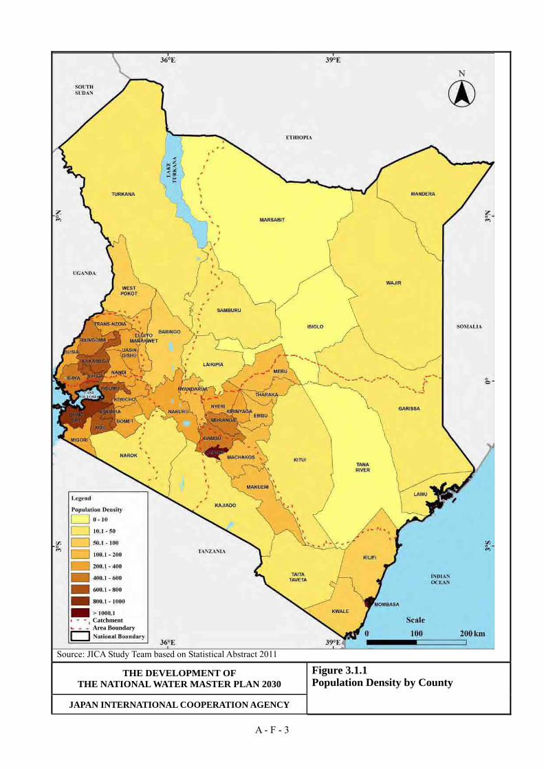
A - F - 3
Source: JICA Study Team based on Statistical Abstract 2011
THE DEVELOPMENT OF THE NATIONAL WATER MASTER PLAN 2030
Figure 3.1.1 Population Density by County
JAPAN INTERNATIONAL COOPERATION AGENCY
Catchment Area Boundary

A - F - 4
Source: JICA Study Team based on 2009 Kenya Population and Housing Census
THE DEVELOPMENT OF THE NATIONAL WATER MASTER PLAN 2030
Figure 3.1.2 Population in Urban and Peri-urban Centres
JAPAN INTERNATIONAL COOPERATION AGENCY

Volume – IV Sectoral Report (1/3)
Sectoral Report (B) Meteorology and Hydrology

Final Report Sectoral Report (B) Meteorology and Hydrology Table of Contents
Nippon Koei Co., Ltd. B - i The Development of the National Water Master Plan 2030
THE PROJECT ON
THE DEVELOPMENT OF THE NATIONAL WATER MASTER PLAN 2030
IN THE REPUBLIC OF KENYA
FINAL REPORT
VOLUME – IV SECTORAL REPORT (1/3)
B: METEOROLOGY AND HYDROLOGY
Abbreviation
Table of Contents
Page
CHAPTER 1 GENERAL HYDROMETEOROLOGY ............................................................. B-1
1.1 Climate ................................................................................................................................. B-1
1.1.1 General Climate ................................................................................................................... B-1 1.1.2 Intertropical Convergence Zone ............................................................................ B-1 1.1.3 Climatic Zone ........................................................................................................ B-2
1.2 Meteorology ......................................................................................................................... B-3 1.2.1 Meteorological Observation .................................................................................. B-3 1.2.2 Temperature .......................................................................................................... B-3 1.2.3 Evaporation and Relative Humidity ...................................................................... B-4 1.2.4 Sunshine Hour ....................................................................................................... B-4 1.2.5 Rainfall .................................................................................................................. B-4
1.3 Hydrology ............................................................................................................................ B-5 1.3.1 Rivers, Lakes and Springs ..................................................................................... B-5 1.3.2 Hydrological Observation ..................................................................................... B-6 1.3.3 Streamflow Gauging Network and Hydrological Database .................................. B-7 1.3.4 Low Flows of Perennial Rivers ............................................................................. B-8 1.3.5 Flood Flows of Perennial Rivers ........................................................................... B-9 1.3.6 Water Quality ...................................................................................................... B-10 1.3.7 Sediment Loads ................................................................................................... B-10 1.3.8 Transboundary Waters ........................................................................................ B-11
CHAPTER 2 ANALYSIS ON CURRENT HYDROMETEOROLOGY ............................... B-12
2.1 Temperature Analysis ........................................................................................................ B-12 2.1.1 Data Collection ................................................................................................... B-12 2.1.2 Generation of Grid Temperature Data ................................................................ B-12 2.1.3 Temperature in the Kenya ................................................................................... B-12

Final Report Table of Contents Sectoral Report (B) Meteorology and Hydrology
The Development of B - ii Nippon Koei Co., Ltd. the National Water Master Plan 2030
2.2 Rainfall Analysis ................................................................................................................ B-13 2.2.1 Data Collection ................................................................................................... B-13 2.2.2 Generation of Grid Rainfall Data ........................................................................ B-13 2.2.3 Annual Rainfall ................................................................................................... B-14 2.2.4 Seasonal and Monthly Rainfall ........................................................................... B-14 2.2.5 Frequency Analysis ............................................................................................. B-15 2.2.6 Number of Rainy Days in a Year ........................................................................ B-16 2.2.7 Annual Rainfall of Drought Year ........................................................................ B-16
CHAPTER 3 TREND ANALYSIS OF METEOROLOGICAL DATA ................................. B-17
3.1 Trend Analysis with Observed Data .................................................................................. B-17
3.2 Available Data .................................................................................................................... B-17
3.3 Trend Analysis of Temperature .......................................................................................... B-18
3.4 Trend Analysis of Rainfall ................................................................................................. B-18
CHAPTER 4 CLIMATE CHANGE ANALYSIS ..................................................................... B-21
4.1 Approach to the Analysis ................................................................................................... B-21
4.2 Scenario of Greenhouse Effect Gas Emission .................................................................... B-22
4.3 General Circulation Models ............................................................................................... B-23 4.3.1 What is a GCM ................................................................................................... B-23 4.3.2 Available Data Set of GCMs .............................................................................. B-23
4.4 Selection of General Circulation Models ........................................................................... B-24 4.4.1 General ................................................................................................................ B-24 4.4.2 Methodology of the Selection ............................................................................. B-24 4.4.3 Selection of GCMs .............................................................................................. B-25
4.5 Bias Correction ................................................................................................................... B-27 4.5.1 Necessity of Bias Correction ............................................................................... B-27 4.5.2 Methodology of Bias Correction ......................................................................... B-27
4.6 Projection of 2030 Climate ................................................................................................ B-32 4.6.1 Data Availability Representing 2030 Climate .................................................... B-32 4.6.2 Methodology of the Projection of 2030 Climate ................................................. B-32
4.7 Evaluation of Uncertainty of Projected Future Climate ..................................................... B-33
4.8 Evaluation of Projected Future Climate in Kenya.............................................................. B-34 4.8.1 Annual Precipitation ........................................................................................... B-34 4.8.2 Seasonal Precipitation ......................................................................................... B-34 4.8.3 Rainfall Frequency .............................................................................................. B-34 4.8.4 Number of Annual Rainy Days ........................................................................... B-35 4.8.5 Number of Seasonal Wet Days ........................................................................... B-35 4.8.6 Annual Rainfall for the Drought Year in 10-Year Return Period ....................... B-35 4.8.7 Seasonal Rainfall for the Drought Year in the 10-Year Return Period ............... B-35 4.8.8 Annual Mean Temperature ................................................................................. B-36

Final Report Sectoral Report (B) Meteorology and Hydrology Table of Contents
Nippon Koei Co., Ltd. B - iii The Development of the National Water Master Plan 2030
4.8.9 Seasonal Mean Temperature ............................................................................... B-36
4.9 Climate Change Impact on Kenya ..................................................................................... B-37 4.9.1 Estimation of Potential Evapotranspiration ........................................................ B-37 4.9.2 Evaluation of Climate Change Impact ................................................................ B-39 4.9.3 Conclusion of the Climate Change Impact Study using GCMs .......................... B-40
4.10 Recommendation for Further Study ................................................................................... B-40
CHAPTER 5 RAINFALL-RUNOFF ANALYSIS ................................................................... B-41
5.1 Approach to the Analysis ................................................................................................... B-41
5.2 SHER Model ...................................................................................................................... B-43 5.2.1 Developing Trail ................................................................................................. B-43 5.2.2 Basic Concept of SHER Model .......................................................................... B-43 5.2.3 Model Components of the SHER Model ............................................................ B-44 5.2.4 Conditions and Parameters .................................................................................. B-49
5.3 Calibration .......................................................................................................................... B-54 5.3.1 Calibration with Observed River Flow Record ................................................... B-54 5.3.2 Verification of Calibrated Model ........................................................................ B-55
5.4 Result of Rainfall-Runoff Analysis .................................................................................... B-58 5.4.1 Simulation of Present and Future Runoff............................................................ B-58 5.4.2 Flow Duration Curve .......................................................................................... B-59 5.4.3 Comparison of Flow Duration Curve .................................................................. B-59
5.5 Impact of Climate Change on Hydrological Conditions .................................................... B-59 5.5.1 Evaluation of Hydrological Water Budget .......................................................... B-59 5.5.2 Soil Evapotranspiration ....................................................................................... B-60 5.5.3 Precipitation Minus Soil Evapotranspiration ...................................................... B-61 5.5.4 Groundwater Recharge ....................................................................................... B-61
5.6 Evaluation of Water Resources .......................................................................................... B-63 5.6.1 Annual Renewable Water Resources .................................................................. B-63 5.6.2 Annual Renewable Surface Water Resources ..................................................... B-64 5.6.3 Annual Renewable Groundwater Resources ....................................................... B-64
5.7 Recommendation for Further Study ................................................................................... B-64
CHAPTER 6 FLOOD ANALYSIS ............................................................................................ B-65
6.1 Approach to the Analysis ................................................................................................... B-65
6.2 Evaluation of Probable Flood Based on Observed Discharge ........................................... B-65 6.2.1 Data Availability and Extraction of Annual Maximum Discharge ..................... B-65 6.2.2 Probable Flood Based on Observed Discharge Record ...................................... B-66
6.3 Assessment of Probable Flood in Future and Regional Area-Flood Curve ....................... B-67
CHAPTER 7 GROUNDWATER ANALYSIS ......................................................................... B-69
7.1 Introduction ........................................................................................................................ B-69

Final Report Table of Contents Sectoral Report (B) Meteorology and Hydrology
The Development of B - iv Nippon Koei Co., Ltd. the National Water Master Plan 2030
7.1.1 Objective ............................................................................................................. B-69 7.1.2 Approach to the Analysis .................................................................................... B-70
7.2 Geology and Hydrogeology ............................................................................................... B-72 7.2.1 Geology ............................................................................................................... B-72 7.2.2 Hydrogeology ..................................................................................................... B-73
7.3 Current Situation of Groundwater Use ............................................................................... B-74
7.4 Conceptual Understanding of Groundwater Flow in Kenya .............................................. B-75 7.4.1 Conceptual Groundwater Flow Model for a Regional Aquifer System .............. B-75 7.4.2 Major Aquifers in Kenya .................................................................................... B-76 7.4.3 Groundwater Recharge and Complex Flow in the Mountain Range .................. B-77
7.5 Preparation for Groundwater Flow Simulation .................................................................. B-79 7.5.1 Available Data .................................................................................................... B-79
7.6 Groundwater Flow Simulation ........................................................................................... B-81 7.6.1 Numerical Simulation of Groundwater Flow ...................................................... B-81
7.7 Estimation of Sustainable Yield ......................................................................................... B-86 7.7.1 Sustainable Yield Rate ........................................................................................ B-86 7.7.2 Renewable Groundwater Recharge ..................................................................... B-86 7.7.3 Method to Estimate Sustainable Yield and Sustainable Yield at Present
(2010) .................................................................................................................. B-87 7.7.4 Estimated Sustainable Yield for the Years 2010, 2030 and 2050 ....................... B-88 7.7.5 Groundwater Balance .......................................................................................... B-88
7.8 Groundwater Survey in Turkana County ........................................................................... B-89
7.9 Recommendations for the Further Study ........................................................................... B-90
CHAPTER 8 LAND USE ANALYSIS ...................................................................................... B-92
8.1 Available Data .................................................................................................................... B-92
8.2 Methodology ...................................................................................................................... B-92
8.3 Land Use Analysis ............................................................................................................. B-94
List of Tables
Page
Table 1.2.1 General Features of Synoptic Stations ................................................................. B-T-1
Table 1.2.2 Observed Items at Synoptic Stations .................................................................... B-T-2
Table 1.3.1 List of River Gauging Stations Used for Analysis in NWMP (1992) .................. B-T-3
Table 1.3.2 List of River Gauging Stations based on Catchment Management Strategies (1/7) – (7/7) ......................................................................................... B-T-3
Table 1.3.3 Surface Water Quality in Six Catchment Areas ................................................... B-T-8
Table 2.1.1 List of Temperature Observation Stations and Data Availability for 1979 - 2010 ................................................................................................................. B-T-9

Final Report Sectoral Report (B) Meteorology and Hydrology Table of Contents
Nippon Koei Co., Ltd. B - v The Development of the National Water Master Plan 2030
Table 2.1.2 List of Rainfall Observation Stations and Those Data Availability for 1979 – 2010 (1/3) - (3/3) .................................................................................. B-T-10
Table 3.2.1 List of Synoptic Stations Used for Calculation .................................................. B-T-13
Table 3.2.2 List of Stations used in NWMP 1992 for Calculation ....................................... B-T-14
Table 4.3.1 List of GCMs and Developers............................................................................ B-T-15
Table 4.4.1 Monthly and Daily Data Availability of GCMs ................................................. B-T-16
Table 4.4.2 Precipitation for 20 years Climatology by Spatial Correlation: Observed Present (Reanalysis) and Simulated Present (20C3M) ...................................... B-T-17
Table 4.4.3 Precipitation for 20 years Climatology by RMSE: Observed Present (Reanalysis) and Simulated Present (20C3M) ................................................... B-T-17
Table 4.4.4 Outgoing Longwave Radiation for 20 years Climatology by Spatial Correlation: Observed Present (Reanalysis) and Simulated Present (20C3M) ............................................................................................................. B-T-18
Table 4.4.5 Outgoing Longwave Radiation for 20 years Climatology by RMSE: Observed Present (Reanalysis) and Simulated Present (20C3M) ...................... B-T-18
Table 4.4.6 Sea Level Pressure for 20 years Climatology by Spatial Correlation: Observed Present (Reanalysis) and Simulated Present (20C3M) ...................... B-T-19
Table 4.4.7 Sea Level Pressure for 20 years Climatology by RMSE: Observed Present (Reanalysis) and Simulated Present (20C3M) ...................................... B-T-19
Table 4.4.8 Surface Air Temperature for 20 years Climatology by Spatial Correlation : Observed Present (Reanalysis) and Simulated Present (20C3M) ............................................................................................................. B-T-20
Table 4.4.9 Surface Air Temperature for 20 years Climatology by RMSE: Observed Present (Reanalysis) and Simulated Present (20C3M) ...................................... B-T-20
Table 4.4.10 Selection of GCMs Used for Calculation ........................................................... B-T-21
Table 5.2.1 Selected Stations for Calibration of SHER Model ............................................. B-T-22
Table 5.3.1 Calibrated Soil Parameter of SHER Model (LVNCA) ...................................... B-T-23
Table 5.3.2 Calibrated Soil Parameter of SHER Model (LVSCA) ....................................... B-T-24
Table 5.3.3 Calibrated Soil Parameter of SHER Model (RVCA) ......................................... B-T-25
Table 5.3.4 Calibrated Soil Parameter of SHER Model (ACA) ........................................... B-T-26
Table 5.3.5 Calibrated Soil Parameter of SHER Model (TCA) ............................................ B-T-27
Table 5.3.6 Calibrated Soil Parameter of SHER Model (ENNCA) ...................................... B-T-28
Table 5.4.1 Present Monthly Average Rainfall by Sub-basin (1/3) – (3/3) .......................... B-T-29
Table 5.4.2 Future Monthly Average Rainfall by Sub-basin (1/3) – (3/3) ............................ B-T-32
Table 5.4.3 Present Monthly Average Naturalised River Discharge by Sub-basin (1/3) – (3/3) ........................................................................................................ B-T-35
Table 5.4.4 Future Monthly Average Naturalised River Discharge by Sub-basin (1/3) – (3/3) ................................................................................................................. B-T-38
Table 6.2.1 Selection of Stations for Frequency Analysis Based on Data Availability (1/2) – (2/2) ........................................................................................................ B-T-41
Table 6.2.2 Annual Maximum Flood Discharge Record (1/2) – (2/2) .................................. B-T-42
Table 6.2.3 Probable Flood Discharge based on Observed Record ...................................... B-T-44

Final Report Table of Contents Sectoral Report (B) Meteorology and Hydrology
The Development of B - vi Nippon Koei Co., Ltd. the National Water Master Plan 2030
Table 6.3.1 Basin Codes and River Names ........................................................................... B-T-45
Table 6.3.2 Regional Area-Flood Curve (1/5) – (5/5) ........................................................... B-T-46
List of Figures
Page
Figure 1.1.1 Climatic Zones of Kenya ..................................................................................... B-F-1
Figure 1.2.1 Location Map of Synoptic .................................................................................... B-F-2
Figure 1.2.2 Mean Monthly Rainfall Depth at Representative Rainfall Gauging Stations from 1979 to 2010 .................................................................................. B-F-3
Figure 1.2.3 Isohyetal Map of Mean Annual Rainfall for 1981 to 2010 .................................. B-F-4
Figure 1.3.1 Major River and Lakes ......................................................................................... B-F-5
Figure 1.3.2 Location of River Flow Gauging Stations ........................................................... B-F-6
Figure 1.3.3 Transboundary Waters ......................................................................................... B-F-7
Figure 2.1.1 Distribution of Temperature Observation Stations Selected and Data Availabilities for 1979 - 2010 .............................................................................. B-F-8
Figure 2.1.2 Mean Annual Temperature for 1981 - 2010......................................................... B-F-9
Figure 2.1.3 Mean Seasonal Temperature for 1981 - 2010 .................................................... B-F-10
Figure 2.1.4 Mean Monthly Temperature for 1981 - 2010 .................................................... B-F-11
Figure 2.2.1 Distribution of Rainfall Observation Stations Selected and Data Availabilities for 1979-2010 .............................................................................. B-F-12
Figure 2.2.2 Mean Annual Rainfall for 1981 - 2010 .............................................................. B-F-13
Figure 2.2.3 Mean Seasonal Rainfall for 1981 - 2010 ............................................................ B-F-14
Figure 2.2.4 Mean Monthly Rainfall for 1981 - 2010 ............................................................ B-F-15
Figure 2.2.5 Frequency Analysis of Daily Rainfall (1/3)-(3/3) .............................................. B-F-16
Figure 2.2.6 Distribution of 1-Day Probable Rainfall Intensity for 1981 - 2010 ................... B-F-19
Figure 2.2.7 Distribution of the 3-Day Probable Rainfall Intensity for 1981 - 2010 ............. B-F-20
Figure 2.2.8 Distribution of the 5-Day Probable Rainfall Intensity for 1981 - 2010 ............. B-F-21
Figure 2.2.9 Annual Number of Rainy Days for 1981 - 2010 ................................................ B-F-22
Figure 2.2.10 Seasonal Rainy Days for 1981 - 2010 ................................................................ B-F-23
Figure 2.2.11 Annual Rainfall of 1/10 Drought Year (1984) for 1981 - 2000 ......................... B-F-24
Figure 2.2.12 Seasonal Rainfall of 1/10 Drought Year ............................................................ B-F-25
Figure 3.2.1 Selected Stations for Trend Analysis ................................................................. B-F-26
Figure 3.2.2 Availability of Temperature Data ...................................................................... B-F-27
Figure 3.2.3 Availability of Rainfall Data .............................................................................. B-F-28
Figure 3.3.1 Spatial Distribution of Temperature Trend ........................................................ B-F-29
Figure 3.3.2 Spatial Distribution of Rainfall Trend (1/2)-(2/2) .............................................. B-F-30

Final Report Sectoral Report (B) Meteorology and Hydrology Table of Contents
Nippon Koei Co., Ltd. B - vii The Development of the National Water Master Plan 2030
Figure 4.4.1 Evaluation of the Reproducibility of GCMs and Selection of the Appropriate Models ........................................................................................... B-F-32
Figure 4.8.1 Spatial Distribution of Mean Annual Rainfall ................................................... B-F-33
Figure 4.8.2 Spatial Distribution of Mean Seasonal Rainfall (MAM) ................................... B-F-34
Figure 4.8.3 Spatial Distribution of Mean Seasonal Rainfall (JJA) ....................................... B-F-35
Figure 4.8.4 Spatial Distribution of Mean Seasonal Rainfall (SON) ..................................... B-F-36
Figure 4.8.5 Spatial Distribution of Mean Seasonal Rainfall (DJF) ....................................... B-F-37
Figure 4.8.6 Spatial Distribution of Daily Rainfall Intensity for 10 Years Return Period ................................................................................................................. B-F-38
Figure 4.8.7 Spatial Distribution of Daily Rainfall Intensity for 50 Years Return Period ................................................................................................................. B-F-39
Figure 4.8.8 Spatial Distribution of Daily Rainfall Intensity for 100 Years Return Period ................................................................................................................. B-F-40
Figure 4.8.9 Spatial Distribution of Number of Rainy Days per Year ................................... B-F-41
Figure 4.8.10 Spatial Distribution of Number of Rainy Days per Season (MAM) .................. B-F-42
Figure 4.8.11 Spatial Distribution of Number of Rainy Days per Season (JJA) ...................... B-F-43
Figure 4.8.12 Spatial Distribution of Number of Rainy Days per Season (SON) .................... B-F-44
Figure 4.8.13 Spatial Distribution of Number of Rainy Days per Season (DJF) ..................... B-F-45
Figure 4.8.14 Spatial Distribution of Mean Annual Rainfall of Drought Year for 10 years Return Period ............................................................................................ B-F-46
Figure 4.8.15 Spatial Distribution of Mean Seasonal Rainfall of Drought Year for 10 Years Return Period (MAM) ............................................................................. B-F-47
Figure 4.8.16 Spatial Distribution of Mean Seasonal Rainfall of Drought Year for 10 Years Return Period (JJA) ................................................................................. B-F-48
Figure 4.8.17 Spatial Distribution of Mean Seasonal Rainfall of Drought Year for 10 Years Return Period (SON) ............................................................................... B-F-49
Figure 4.8.18 Spatial Distribution of Mean Seasonal Rainfall of Drought Year for 10 Years Return Period (DJF) ................................................................................. B-F-50
Figure 4.8.19 Spatial Distribution of Mean Annual Surface Air Temperature ........................ B-F-51
Figure 4.8.20 Spatial Distribution of Mean Seasonal Surface Air Temperature (MAM) ........ B-F-52
Figure 4.8.21 Spatial Distribution of Mean Seasonal Surface Air Temperature (JJA) ............ B-F-53
Figure 4.8.22 Spatial Distribution of Mean Seasonal Surface Air Temperature (SON) .......... B-F-54
Figure 4.8.23 Spatial Distribution of Mean Seasonal Surface Air Temperature (DJF) ............ B-F-55
Figure 4.9.1 Spatial Distribution of Mean Annual Potential Evapotranspiration (Hamon Method) ................................................................................................ B-F-56
Figure 4.9.2 Spatial Distribution of Mean Seasonal Potential Evapotranspiration (MAM, Hamon Method) .................................................................................... B-F-57
Figure 4.9.3 Spatial Distribution of Mean Seasonal Potential Evapotranspiration (JJA, Hamon Method) ................................................................................................. B-F-58
Figure 4.9.4 Spatial Distribution of Mean Seasonal Potential Evapotranspiration (SON, Hamon Method) ...................................................................................... B-F-59

Final Report Table of Contents Sectoral Report (B) Meteorology and Hydrology
The Development of B - viii Nippon Koei Co., Ltd. the National Water Master Plan 2030
Figure 4.9.5 Spatial Distribution of Mean Seasonal Potentia Evapotranspiration (DJF, Hamon Method) ................................................................................................. B-F-60
Figure 4.9.6 Spatial Distribution of Mean Annual Potential Evapotranspiration (FAO Penman – Monteith Method) ............................................................................. B-F-61
Figure 4.9.7 Spatial Distribution of Mean Seasonal Potential Evapotranspiration (MAM, FAO Penman – Monteith Method) ....................................................... B-F-62
Figure 4.9.8 Spatial Distribution of Mean Seasonal Potential Evapotranspiration (JJA, FAO Penman – Monteith Method) .................................................................... B-F-63
Figure 4.9.9 Spatial Distribution of Mean Seasonal Potential Evapotranspiration (SON, FAO Penman – Monteith Method) ......................................................... B-F-64
Figure 4.9.10 Spatial Distribution of Mean Seasonal Potential Evapotranspiration (DJF, FAO Penman – Monteith Method) .................................................................... B-F-65
Figure 4.9.11 Spatial Distribution of Mean Annual P-PET (Hamon Method) ......................... B-F-66
Figure 4.9.12 Spatial Distribution of Mean Seasonal P-PET (MAM, Hamon Method) .......... B-F-67
Figure 4.9.13 Spatial Distribution of Mean Seasonal P-PET (JJA, Hamon Method) .............. B-F-68
Figure 4.9.14 Spatial Distribution of Mean Seasonal P-PET (SON, Hamon Method) ............ B-F-69
Figure 4.9.15 Spatial Distribution of Mean Seasonal P-PET (DJF, Hamon Method) .............. B-F-70
Figure 4.9.16 Spatial Distribution of Mean Annual P-PET (FAO Penman – Monteith Method) .............................................................................................................. B-F-71
Figure 4.9.17 Spatial Distribution of Mean Seasonal P-PET (MAM, FAO Penman – Monteith Method) .............................................................................................. B-F-72
Figure 4.9.18 Spatial Distribution of Mean Seasonal P-PET (JJA, FAO Penman – Monteith Method) .............................................................................................. B-F-73
Figure 4.9.19 Spatial Distribution of Mean Seasonal P-PET (SON, FAO Penman – Monteith Method) .............................................................................................. B-F-74
Figure 4.9.20 Spatial Distribution of Mean Seasonal P-PET (DJF, FAO Penman – Monteith Method) .............................................................................................. B-F-75
Figure 5.2.1 Reviewed Sub Catchment Boundaries and WRMA Catchment Areas .............. B-F-76
Figure 5.2.2 Surface Blocks of SHER Model LVN-1 ............................................................ B-F-77
Figure 5.2.3 Surface Blocks of SHER Model LVN-2 ............................................................ B-F-78
Figure 5.2.4 Surface Blocks of SHER Model LVN-3 ............................................................ B-F-79
Figure 5.2.5 Surface Blocks of SHER Model LVN-4 ............................................................ B-F-80
Figure 5.2.6 Surface Blocks of SHER Model LVN-5 ............................................................ B-F-81
Figure 5.2.7 Surface Blocks of SHER Model LVN-6 ............................................................ B-F-82
Figure 5.2.8 Surface Blocks of SHER Model LVS-1 ............................................................. B-F-83
Figure 5.2.9 Surface Blocks of SHER Model LVS-2 ............................................................. B-F-84
Figure 5.2.10 Surface Blocks of SHER Model LVS-3 ............................................................. B-F-85
Figure 5.2.11 Surface Blocks of SHER Model LVS-4 ............................................................. B-F-86
Figure 5.2.12 Surface Blocks of SHER Model RV-1 ............................................................... B-F-87
Figure 5.2.13 Surface Blocks of SHER Model RV-2 ............................................................... B-F-88
Figure 5.2.14 Surface Blocks of SHER Model RV-3 ............................................................... B-F-89

Final Report Sectoral Report (B) Meteorology and Hydrology Table of Contents
Nippon Koei Co., Ltd. B - ix The Development of the National Water Master Plan 2030
Figure 5.2.15 Surface Blocks of SHER Model RV-4 ............................................................... B-F-90
Figure 5.2.16 Surface Blocks of SHER Model RV-5 ............................................................... B-F-91
Figure 5.2.17 Surface Blocks of SHER Model RV-6 ............................................................... B-F-92
Figure 5.2.18 Surface Blocks of SHER Model AT-1 ............................................................... B-F-93
Figure 5.2.19 Surface Blocks of SHER Model AT-2 ............................................................... B-F-94
Figure 5.2.20 Surface Blocks of SHER Model AT-3 ............................................................... B-F-95
Figure 5.2.21 Surface Blocks of SHER Model AT-4 ............................................................... B-F-96
Figure 5.2.22 Surface Blocks of SHER Model AT-5 ............................................................... B-F-97
Figure 5.2.23 Surface Blocks of SHER Model TN-1 ............................................................... B-F-98
Figure 5.2.24 Surface Blocks of SHER Model TN-2 ............................................................... B-F-99
Figure 5.2.25 Surface Blocks of SHER Model TN-3 ............................................................. B-F-100
Figure 5.2.26 Surface Blocks of SHER Model TN-4 ............................................................. B-F-101
Figure 5.2.27 Surface Blocks of SHER Model TN-5 ............................................................. B-F-102
Figure 5.2.28 Surface Blocks of SHER Model EN-1 ............................................................. B-F-103
Figure 5.2.29 Surface Blocks of SHER Model EN-2 ............................................................. B-F-104
Figure 5.2.30 Surface Blocks of SHER Model EN-3 ............................................................. B-F-105
Figure 5.2.31 Surface Blocks of SHER Model EN-4 ............................................................. B-F-106
Figure 5.2.32 Surface Blocks of SHER Model EN-5 ............................................................. B-F-107
Figure 5.2.33 Surface Blocks of SHER Model EN-6 ............................................................. B-F-108
Figure 5.2.34 Soil Type Classification for SHER Model ....................................................... B-F-109
Figure 5.2.35 River Gauging Stations Selected for Calibration of SHER Model .................. B-F-110
Figure 5.3.1 Summary of Calibration Result ........................................................................ B-F-111
Figure 5.3.2 Comparison of Simulated Discharge and Observed Discharge (1/6)-(6/6) ..... B-F-112
Figure 5.4.1 Comparison of Flow Duration Curves for Present and Futures Climate (1/5)-(5/5) ......................................................................................................... B-F-118
Figure 5.5.1 Annual Water Budget (Hamon Method) (1/4)-(4/4) ........................................ B-F-123
Figure 5.5.2 Annual Water Budget (FAO Penman – Monteith Method) (1/4)-(4/4) ........... B-F-127
Figure 5.5.3 Annual Runoff Volume (Based on 1981-2000) ............................................... B-F-131
Figure 5.5.4 Spatial Distribution of Mean Annual SET (Hamon Method) .......................... B-F-132
Figure 5.5.5 Spatial Distribution of Mean Seasonal SET (MAM, Hamon Method) ............ B-F-133
Figure 5.5.6 Spatial Distribution of Mean Seasonal SET (JJA, Hamon Method) ................ B-F-134
Figure 5.5.7 Spatial Distribution of Mean Seasonal SET (SON, Hamon Method) .............. B-F-135
Figure 5.5.8 Spatial Distribution of Mean Seasonal SET (DJF, Hamon Method) ............... B-F-136
Figure 5.5.9 Spatial Distribution of Mean Annual SET (FAO Penman – Monteith Method) ............................................................................................................ B-F-137
Figure 5.5.10 Spatial Distribution of Mean Seasonal SET (MAM, FAO Penman – Monteith Method) ............................................................................................ B-F-138
Figure 5.5.11 Spatial Distribution of Mean Seasonal SET (JJA, FAO Penman – Monteith Method) ............................................................................................ B-F-139

Final Report Table of Contents Sectoral Report (B) Meteorology and Hydrology
The Development of B - x Nippon Koei Co., Ltd. the National Water Master Plan 2030
Figure 5.5.12 Spatial Distribution of Mean Seasonal SET (SON, FAO Penman – Monteith Method) ............................................................................................ B-F-140
Figure 5.5.13 Spatial Distribution of Mean Seasonal SET (DJF, FAO Penman – Monteith Method) ............................................................................................ B-F-141
Figure 5.5.14 Spatial Distribution of Mean Annual P-SET (Hamon Method) ....................... B-F-142
Figure 5.5.15 Spatial Distribution of Mean Seasonal P- SET (MAM, Hamon Method) ....... B-F-143
Figure 5.5.16 Spatial Distribution of Mean Seasonal P- Soil ET (JJA, Hamon Method) ...... B-F-144
Figure 5.5.17 Spatial Distribution of Mean Seasonal P- SET (SON, Hamon Method) ......... B-F-145
Figure 5.5.18 Spatial Distribution of Mean Seasonal P- SET (DJF, Hamon Method) ........... B-F-146
Figure 5.5.19 Spatial Distribution of Mean Annual P- SET (FAO Penman – Monteith Method) ............................................................................................................ B-F-147
Figure 5.5.20 Spatial Distribution of Mean Seasonal P- SET (MAM, FAO Penman – Monteith Method) ............................................................................................ B-F-148
Figure 5.5.21 Spatial Distribution of Mean Seasonal P- SET (JJA, FAO Penman – Monteith Method) ............................................................................................ B-F-149
Figure 5.5.22 Spatial Distribution of Mean Seasonal P- Soil ET (SON, FAO Penman – Monteith Method) ............................................................................................ B-F-150
Figure 5.5.23 Spatial Distribution of Mean Seasonal P- SET (DJF, FAO Penman – Monteith Method) ............................................................................................ B-F-151
Figure 5.5.24 Spatial Distribution of Mean Annual Groundwater Recharge (Hamon Method) ............................................................................................................ B-F-152
Figure 5.5.25 Spatial Distribution of Mean Seasonal Groundwater Recharge (MAM, Hamon Method) ............................................................................................... B-F-153
Figure 5.5.26 Spatial Distribution of Mean Seasonal Groundwater Recharge (JJA, Hamon Method) ............................................................................................... B-F-154
Figure 5.5.27 Spatial Distribution of Mean Seasonal Groundwater Recharge (SON, Hamon Method) ............................................................................................... B-F-155
Figure 5.5.28 Spatial Distribution of Mean Seasonal Groundwater Recharge (DJF, Hamon Method) ............................................................................................... B-F-156
Figure 5.5.29 Spatial Distribution of Mean Annual Groundwater Recharge (FAO Penman – Monteith Method) ........................................................................... B-F-157
Figure 5.5.30 Spatial Distribution of Mean Seasonal Groundwater Recharge (MAM, FAO Penman – Monteith Method) .................................................................. B-F-158
Figure 5.5.31 Spatial Distribution of Mean Seasonal Groundwater Recharge (JJA, FAO Penman – Monteith Method) .................................................................. B-F-159
Figure 5.5.32 Spatial Distribution of Mean Seasonal Groundwater Recharge (SON, FAO Penman – Monteith Method) .................................................................. B-F-160
Figure 5.5.33 Spatial Distribution of Mean Seasonal Groundwater Recharge (DJF, FAO Penman – Monteith Method) .................................................................. B-F-161
Figure 5.6.1 Specific Renewable Surface Water Resources by Sub Basin in Present Climatology ...................................................................................................... B-F-162
Figure 5.6.2 Difference of Future Annual Runoff and Present Annual Runoff by Sub Basin ................................................................................................................ B-F-163
Figure 6.2.1 Availability of Observed River Flow (1AH01,Sio) ......................................... B-F-164

Final Report Sectoral Report (B) Meteorology and Hydrology Table of Contents
Nippon Koei Co., Ltd. B - xi The Development of the National Water Master Plan 2030
Figure 6.2.2 Availability of Observed River Flow (1BG07, Rongai) .................................. B-F-165
Figure 6.2.3 Availability of Observed River Flow (1EF01, Nzoia at Ruambwa) ................ B-F-166
Figure 6.2.4 Availability of Observed River Flow (1GB05, Ainamatua) ............................ B-F-167
Figure 6.2.5 Availability of Observed River Flow (1GC04, Tugenon) ................................ B-F-168
Figure 6.2.6 Availability of Observed River Flow (1GG01, Namuting) .............................. B-F-169
Figure 6.2.7 Availability of Observed River Flow (1LA03, Nyangores) ............................. B-F-170
Figure 6.2.8 Availability of Observed River Flow (3DA02, Athi Munyu) .......................... B-F-171
Figure 6.2.9 Availability of Observed River Flow (4BC02, Tana Sagana).......................... B-F-172
Figure 6.2.10 Availability of Observed River Flow (4BE01, Maragua) ................................ B-F-173
Figure 6.2.11 Availability of Observed River Flow (4CB04, Thika) ..................................... B-F-174
Figure 6.2.12 Availability of Observed River Flow (4DA10, Thiba) .................................... B-F-175
Figure 6.2.13 Availability of Observed River Flow (4DC03, Rupingazi) ............................. B-F-176
Figure 6.2.14 Availability of Observed River Flow (4EA07, Mutonga) ................................ B-F-177
Figure 6.2.15 Availability of Observed River Flow (4F13, Grand Falls) .............................. B-F-178
Figure 6.2.16 Availability of Observed River Flow (4G01, Garissa) .................................... B-F-179
Figure 6.2.17 Availability of Observed River Flow (5BB02, Ewaso Ng’iro) ........................ B-F-180
Figure 6.2.18 Availability of Observed River Flow (5E03, Ewaso Ng’iro at Archers’ Post) ................................................................................................................. B-F-181
Figure 7.2.1 Geological Map of Kenya ................................................................................ B-F-182
Figure 7.3.1 Location of Existing Boreholes ........................................................................ B-F-183
Figure 7.3.2 Histograms of Borehole Numbers by Construction Year (1/2)-(2/2) ............... B-F-184
Figure 7.3.3 Histograms of Borehole Numbers by Depth (1/2)-(2/2) .................................. B-F-186
Figure 7.3.4 Histograms of Borehole Numbers by Yield (1/2)-(2/2) ................................... B-F-188
Figure 7.4.1 Groundwater Resources Map of Kenya (UNESCO) ........................................ B-F-190
Figure 7.5.1 Hydrogeological Classification ........................................................................ B-F-191
Figure 7.5.2 Histograms of Hydraulic Conductivity by Hydrogeological Classification .................................................................................................... B-F-192
Figure 7.5.3 Spatial Distribution of Hydraulic Conductivity ............................................... B-F-193
Figure 7.5.4 Locations of Existing Production Wells and Average Well Depths ................ B-F-194
Figure 7.5.5 Thickness of the Main Aguifer ........................................................................ B-F-195
Figure 7.5.6 Groundwater Level Contour Map .................................................................... B-F-196
Figure 7.6.1 Boundary Conditions for the Aquifer System .................................................. B-F-197
Figure 7.6.2 Structure of the Aquifer and Hydraulic Conductivities ................................... B-F-198
Figure 7.6.3 Spatial Distribution of Percolation ................................................................... B-F-199
Figure 7.6.4 Water Budget near the Ground Surface and Groundwater Evapotranspiration ........................................................................................... B-F-200
Figure 7.6.5 Spatial Distribution of Potential Ground Water Evapotranspiration ............... B-F-201
Figure 7.6.6 Groundwater Contour Map Estimated and Observed Contours ....................... B-F-202

Final Report Table of Contents Sectoral Report (B) Meteorology and Hydrology
The Development of B - xii Nippon Koei Co., Ltd. the National Water Master Plan 2030
Figure 7.6.7 Spatial Distribution of Groundwater Evapotranspiration ................................. B-F-203
Figure 7.6.8 Groundwater Tables within 5m and 20m Depths below Ground Surface ....... B-F-204
Figure 7.6.9 Distribution of Rivers ....................................................................................... B-F-205
Figure 7.6.10 Locations of Groundwater Evapotranspiration in Forest Land (1/2)-(2/2) ...... B-F-206
Figure 7.6.11 Locations of Groundwater Evapotranspiration in Agriculture Land (1/2) -(2/2) ........................................................................................................ B-F-208
Figure 7.6.12 Locations of Groundwater Evapotranspiration in Shrub/Wood Land (1/2) -(2/2) ........................................................................................................ B-F-210
Figure 7.6.13 Locations of Groundwater Evapotranspiration in Grass Land (1/2) -(2/2) ...... B-F-212
Figure 7.6.14 Locations of Groundwater Evapotranspiration in Savannah Land (1/2) -(2/2) ........................................................................................................ B-F-214
Figure 7.6.15 Locations of Groundwater Evapotranspiration in Bare Land (1/2) -(2/2) ........ B-F-216
Figure 7.7.1 Sustainable Yield of Groundwater Excluding Locations with Rivers ............. B-F-218
Figure 7.7.2 Sustainable Yield of Groundwater Including Locations with Rivers ............... B-F-219
Figure 7.7.3 Sustainable Yield of Groundwater excluding Locations in Discharge Aera .................................................................................................................. B-F-220
Figure 7.7.4 Sustainable Yield of Groundwater (2030) ....................................................... B-F-221
Figure 7.7.5 Sustainable Yield of Groundwater (2050) ....................................................... B-F-222
Figure 7.7.6 Estimated Present Groundwater Abstraction Rate Map ................................... B-F-223
Figure 7.7.7 Present Groundwater Balance Map .................................................................. B-F-224
Figure 7.7.8 Location of Groundwater Resources Survey in Trukana County .................... B-F-225
Figure 8.3.1 Land Use Map of Kenya in 1990 ..................................................................... B-F-226
Figure 8.3.2 Land Use Map of Kenya in 2010 ..................................................................... B-F-227

Final Report Sectoral Report (B) Meteorology and Hydrology Abbreviations
Nippon Koei Co., Ltd. B - I The Development of the National Water Master Plan 2030
List of Abbreviations and Acronyms
AR4 : Fourth Assessment Report ASAL : arid and semi-arid land CBS : Central Bureau of Statistics CDF : Cumulative Distribution Function CMIP3 : Phase 3 of Coupled Model Intercomparison Project CMS Catchment Management Strategy DEM : digital elevation model DIAS : Data Integration and Analysis System
EDITORIA : University of Tokyo Earth Observation Data Integration and Fusion Research Initiative
ENN : Ewaso Ng'iro North ENSO : El-Niño/Southern Oscillation ESRL PSD : Earth System Research Laboratory Physical Sciences Division FAO : Food and Agriculture Organization GCM : General Circulation Model GEV : Generalized Extreme Value Distribution GEWEX : Global Energy and Water Cycle Experiment GPCP : Global Precipitation Climatology Project GW : Groundwater GWEVT Groundwater Evapotranspiration IPCC : Intergovernmental Panel on Climate Change ITCZ : Inter Tropical Convergence Zone JICA : Japan International Cooperation Agency KMD : Kenya Meteorological Department LN3 : Log Normal Distribution LP3 : Log Pearson III Distribution LVN : Lake Victoria North LVS : Lake Victoria South MWI : Ministry of Water and Irrigation NASA : National Aeronautics and Space Administration NCEP : National Centers for Environmental Prediction NOAA : National Oceanic and Atmospheric Administration NWMP : National Water Master Plan OAR : Office of Air and Radiation OLR : Outgoing Longwave Radiation PCMDI : Program for Climate Model Diagnosis and Intercomparison PDF : Probability Density Function PET : potential evapotranspiration RFA : rainfall frequency analysis RGB : Red Green Blue RGS river gauging station RMS : root mean square RMSE : root mean square error RV : Rift Valley SHER : Similar Hydrologic Element Response

Final Report Abbreviations Sectoral Report (B) Meteorology and Hydrology
The Development of B - II Nippon Koei Co., Ltd. the National Water Master Plan 2030
SLSC : Standard Least-squares Criterion SQL : Structured Query Language SQRT-ET : Square-Root Exponential Type SRES : Special Report on Emission Scenarios SRTM : Shuttle Rader Topography Mission SWIR : short wave infrared TAR : Third Assessment Report TC : Tropical Cyclone
TGICA : Task Group on Data and Scenario Support for Impact and Climate Assessment
TM : Thematic Mapper UNEP : United Nations Environment Programme UNESCO : United Nations Educational, Scientific and Cultural Organization UTM : Universal Transverse Mercator VNIR : visible and near infrared WCRP : World Climate Research Programme WGCM : Working Group on Coupled Modelling WHYMAP : Worldwide Hydrogeological Mapping and Assessment Programme WRMA : Water Resource Management Authority

Final Report Sectoral Report (B) Meteorology and Hydrology Abbreviations
Nippon Koei Co., Ltd. B - III The Development of the National Water Master Plan 2030
Abbreviations of Measures
Length mm = millimeter cm = centimeter m = meter km = kilometer
Money KSh = Kenya shilling US$ = U.S. dollar
Area ha = hectare m2 = square meter km2 = square kilometer
Energy kcal = Kilocalorie kW = kilowatt MW = megawatt kWh = kilowatt-hour GWh = gigawatt-hour
Volume 1, lit = liter m3 = cubic meter m3/s, cms = cubic meter per second CM = cubic meter MCM = million cubic meter BCM = billion cubic meter m3/d, cmd = cubic meter per day BBL = Barrel
Others % = percent o = degree ' = minute " = second °C = degree Celsius cap. = capital LU = livestock unit md = man-day mil. = million no. = number pers. = person mmho = micromho ppm = parts per million ppb = parts per billion lpcd = litter per capita per day
Weight mg = milligram g = gram kg = kilogram t = ton MT = metric ton Time s = second hr = hour d = day yr = year

NOTE 1. The National Water Master Plan 2030 was prepared based on the material and data provided from
Kenyan Government and its relevant organisations during field surveys in Kenya carried out until November 2012. The sources etc. of the material and data utilised for the study are described in the relevant part of the reports.
2. The names of ministries and related organisations of Kenyan Government are as of November 2012.
3. Information to be updated
The following information which is given in the report is needed to be updated properly:
(1) Information on the proposed development projects
The features and implementation schedules of the proposed development projects may be changed toward implementation of the project. After the subject projects were clearly featured for implementation, the project features and implementation schedules in this report should be updated.
(2) Information on the water demand
The water demand projected in this master plan should be revised when the large scale development plans, other than the projects proposed in this master plan, were formulated, as they will significantly affect to the water resources development and management.
4. Exchange rate for cost estimate
The costs of the proposed development and management plans were estimated by applying the following exchange rate as of November 1, 2012.
EXCHANGE RATE
US$1.00 = KSh 85.24 = ¥79.98 as of November 1, 2012

Final Report General Hydrometeorology Sectoral Report (B) Meteorology and Hydrology Chapter 1
Nippon Koei Co., Ltd. B - 1 The Development of the National Water Master Plan 2030
CHAPTER 1 GENERAL HYDROMETEOROLOGY
1.1 Climate
1.1.1 General Climate
Kenya lies approximately between latitudes 5°20'N and 4°40'S and between longitudes 33°50'E and 41°45'E. Regional factors, which modify rainfall over most parts of Kenya, include large bodies of water bodies Lake Victoria, complex topography such as the Great Rift Valley, and high mountains such Mt. Kenya and such as Mt. Elgon. Local factors such as land-sea breezes and vegetation further complicates the rainfall distribution.
A relatively wet and narrow tropical belt lies along the coast of the Indian Ocean. Behind the coastline are large areas of semi-arid and arid lands. The land then rises steeply to a highland plateau through which the Rift Valley runs. Kenya generally experiences two seasonal rainfall peaks (bimodal) in most places. However, some stations in the western and central parts of the Rift Valley experience a tri-modal rainfall pattern.
There are four seasons in Kenya as described in the following table.
Month Season December – February (DJF) - March – May (MAM) Long Rain June – August (JJA) - September – November (SON) Short Rain
Source: KMD
1.1.2 Intertropical Convergence Zone
The climate in Kenya is controlled by the northward and southward movement of the Intertropical Convergence Zone (ITCZ). The ITCZ is the area encircling the earth near the equator where winds originating in the northern and southern hemispheres come together.
Source: JICA Study Team
Schematic Image of Global Belts of High and Low Pressure and ITCZ
Variation in the location of ITCZ drastically affects the rainfall in Kenya. Long term changes in the ITCZ may result in severe droughts or floods.
High Pressure Zone
Low Pressure Zone
Low Pressure Zone
Low Pressure ZoneITCZEquater
High Pressure Zone
Northeast Trades
Southeast Trades
HadleyCell
FerrelCell
FerrelCell
PolarCell
HadleyCell

General Hydrometeorology Final Report Chapter 1 Sectoral Report (B) Meteorology and Hydrology
The Development of B - 2 Nippon Koei Co., Ltd. the National Water Master Plan 2030
1.1.3 Climatic Zone
The bimodal nature of rainfall corresponds with the northward and southward migration of the ITCZ. The first peak or season termed as the “long-rains” in the East African region occurs from March to May, while the second season termed as the “short-rains” is observed from October to December. However, the western parts of the country, receive considerable rainfall during the month of June to September season. This is associated with the incursion of the Congo air mass. This period from January to February is generally dry over most parts of the country. Northeasterly monsoons, which are dominant at this time, are difluent and dry (Griffiths, 1972, Anyamba, 1983).
The main synoptic scale systems affecting rainfall in Kenya are the followings:
The position and strength of subtropical high-pressure systems in the Southwest Indian Ocean (Mascarene High), Southeast Atlantic Ocean (St Helena High), North Atlantic Ocean (Azores/Saharan High), and the Arabian High to the northeast.
The position and intensity of the ITCZ. The position and intensity of tropical cyclones (TCs). El-Niño/Southern Oscillation (ENSO). The Congo air mass. Inter-seasonal annual waves: the quasi-biennial oscillations (QBO).
The moisture availability (ratio of rainfall and potential evaporation) of Kenya is presented in the climatic zones of Kenya as Figure 1.1.1. The moisture availability zones are divided into I-IV: (I) >80-Humid, (II) 65-80-Sub-humid, (III) 50-65-Semi-humid, (IV) 40-50-Semi-humid to Semi-arid, (V) 25-40-Semi-arid, (VI) 15-25-Arid, and (VII) <15-Very arid. The temperature zones are divided into 1-9: (1) 24-30, (2) 22-24, (3) 20-22, (4) 18-20, (5) 16-18, (6) 14-16, (7) 12-14, (8) 10-12, and (9) Less than 10.
Similar to the agro-climatic zones of Kenya, the Kenya Meteorological Department (KMD) defines the climatic zones in Kenya into 12 zones as described in the following table and the figure on right. Source: KMD
Climatic Zone of Kenya Climatic Zone of Kenya defined by KMD
Area Climatic Zone Representative Station 1 North Western Kenya Arid (VI) to Very Arid (VII) Lodwar 2 Northern Kenya Arid (VI) to Very Arid (VII) Marsabit, Moyale 3 North Eastern Kenya Arid (VI) to Very Arid (VII) Mandera, Wajir, Garissa 4 Southern Lowlands Semi Arid (V) To Arid (VI) Voi 5 Northern Coast Strip Semi-Humid (III) to Semi-Arid (V) Lamu 6 Southern Coast Strip Semi-Humid (III) to Semi-Arid (V) Mombasa, Mtwapa, Malindi, Msabaha 7 South Eastern Lowlands Semi Arid (V) To Arid (VI) Machakos, Makindu
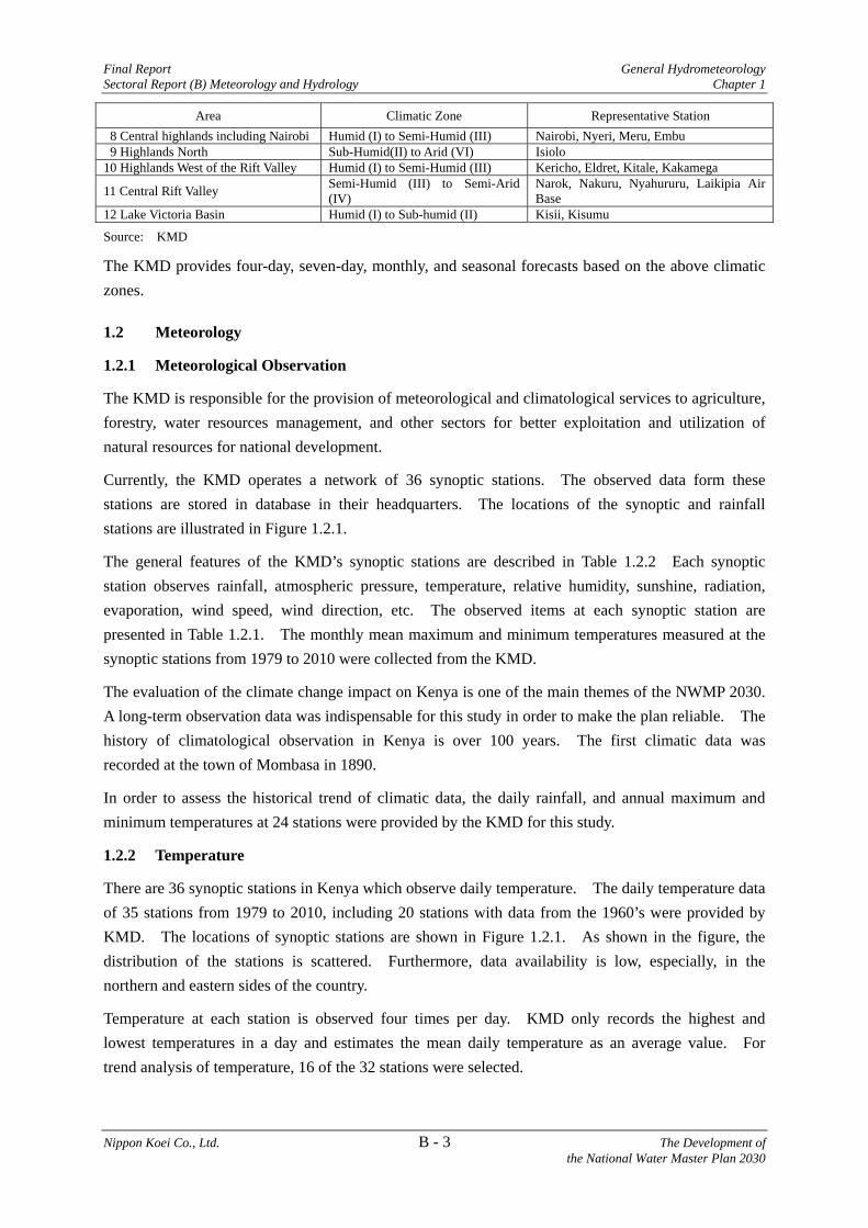
Final Report General Hydrometeorology Sectoral Report (B) Meteorology and Hydrology Chapter 1
Nippon Koei Co., Ltd. B - 3 The Development of the National Water Master Plan 2030
Area Climatic Zone Representative Station 8 Central highlands including Nairobi Humid (I) to Semi-Humid (III) Nairobi, Nyeri, Meru, Embu 9 Highlands North Sub-Humid(II) to Arid (VI) Isiolo
10 Highlands West of the Rift Valley Humid (I) to Semi-Humid (III) Kericho, Eldret, Kitale, Kakamega
11 Central Rift Valley Semi-Humid (III) to Semi-Arid (IV)
Narok, Nakuru, Nyahururu, Laikipia Air Base
12 Lake Victoria Basin Humid (I) to Sub-humid (II) Kisii, Kisumu
Source: KMD
The KMD provides four-day, seven-day, monthly, and seasonal forecasts based on the above climatic zones.
1.2 Meteorology
1.2.1 Meteorological Observation
The KMD is responsible for the provision of meteorological and climatological services to agriculture, forestry, water resources management, and other sectors for better exploitation and utilization of natural resources for national development.
Currently, the KMD operates a network of 36 synoptic stations. The observed data form these stations are stored in database in their headquarters. The locations of the synoptic and rainfall stations are illustrated in Figure 1.2.1.
The general features of the KMD’s synoptic stations are described in Table 1.2.2 Each synoptic station observes rainfall, atmospheric pressure, temperature, relative humidity, sunshine, radiation, evaporation, wind speed, wind direction, etc. The observed items at each synoptic station are presented in Table 1.2.1. The monthly mean maximum and minimum temperatures measured at the synoptic stations from 1979 to 2010 were collected from the KMD.
The evaluation of the climate change impact on Kenya is one of the main themes of the NWMP 2030. A long-term observation data was indispensable for this study in order to make the plan reliable. The history of climatological observation in Kenya is over 100 years. The first climatic data was recorded at the town of Mombasa in 1890.
In order to assess the historical trend of climatic data, the daily rainfall, and annual maximum and minimum temperatures at 24 stations were provided by the KMD for this study.
1.2.2 Temperature
There are 36 synoptic stations in Kenya which observe daily temperature. The daily temperature data of 35 stations from 1979 to 2010, including 20 stations with data from the 1960’s were provided by KMD. The locations of synoptic stations are shown in Figure 1.2.1. As shown in the figure, the distribution of the stations is scattered. Furthermore, data availability is low, especially, in the northern and eastern sides of the country.
Temperature at each station is observed four times per day. KMD only records the highest and lowest temperatures in a day and estimates the mean daily temperature as an average value. For trend analysis of temperature, 16 of the 32 stations were selected.

General Hydrometeorology Final Report Chapter 1 Sectoral Report (B) Meteorology and Hydrology
The Development of B - 4 Nippon Koei Co., Ltd. the National Water Master Plan 2030
Kenya has a wide variety of temperature which ranges from below the freezing point on the snow-capped Mt. Kenya as a minimum to over 40 °C in the north and northeast arid and semi-arid areas as
maximum. The approximate temperature in the coastal town of Mombasa (altitude 17 m) is 30.3 oC at maximum and 22.4 oC at minimum; the capital city Nairobi (altitude 1,661 m) 25.2 oC at maximum and 13.6oC at minimum; Eldoret (altitude 2,085 m) 23.6 oC at maximum and 9.5 oC at minimum; and Lodwar (altitude 506 m) and the drier north plain lands 34.8 oC at maximum and 23.7 oC at minimum.
1.2.3 Evaporation and Relative Humidity
The mean annual evaporation depth varies from 1,215 mm at Kimakia forest station to 3,945 mm at Lokori in South Turkana. The estimation of evaporation rates from water surface is important for water resources development, especially in arid and semi-arid land (ASAL) regions.
The potential evapotranspiration evaluated using Harmon’s equation and FAO Penman-Monteith method was discussed in Chapter 2.
The highest annual mean maximum and minimum relative humidities were both recorded at the Mombasa station at approximately 90% and 82%, respectively. On the other hand, the lowest annual mean maximum and minimum humidities were recorded at the Lodwar station at approximately 60% and 34%, respectively.
1.2.4 Sunshine Hour
The mean sunshine hours are approximately 7-8 hours. Lodwar has the longest mean monthly sunshine hour with 10.3 hours in September. On the other hand, the shortest mean monthly sunshine hour was recorded in Dagoretti station with 3.0 hours in July.
1.2.5 Rainfall
The average annual rainfall over the country is approximately 680 mm. It varies from 0 to about 250 mm in the ASAL zone areas such as Garissa, Isiolo, Mandera, Marsabit, Moyale, and Turkana to 2,000 mm in high rainfall zones such as Nyeri, Meru, Nyandarua, and Mt. Elgon regions. The high rainfall zone, which receives more than 1,000 mm of annual rainfall, occupies less than 20% of the productive agricultural land and carries approximately 50% of the country’s population. Most of the food and cash crops as well as livestock are produced in this zone under semi-intensive and intensive systems. The medium rainfall zone receives between 750-1000 mm of rainfall annually and occupies between 30-35% of the country’s land area. It is home to about 30% of the population. Farmers in this zone keep cattle and small stock, and grow drought-tolerant crops. The ASALs, which receive 200 to 750 mm of rainfall annually, cover over 80% of the total area. They are not suited for rainfed agriculture due to low and erratic rainfall, although there is cultivation of some crops.
The mean monthly rainfall depth recorded at each station is shown in Figure 1.2.2. An isohyetal map of mean annual rainfall depth for the data from 1981 to 2010 is shown in Figure 1.2.3.

Final Report General Hydrometeorology Sectoral Report (B) Meteorology and Hydrology Chapter 1
Nippon Koei Co., Ltd. B - 5 The Development of the National Water Master Plan 2030
1.3 Hydrology
1.3.1 Rivers, Lakes and Springs
(1) Rivers
The major rivers in Kenya are shown in Figure 1.3.1. Kenya's river system is relatively simple. All the main rivers are consequent on the great dome formed by the Central Highlands.
Kenya has five “water towers”, namely, Mt. Kenya (199,558 ha), Aberdares Range (103,315 ha), Cherangani Hills (128,000 ha), Mt. Elgon (73,089 ha), and Mau Forest Complex (400,000 ha). The water towers from the upper catchments of all the main perennial rivers in Kenya. On the other hand, the rivers in ASALS run out seasonally when heavy storm rainfall occurs.
Kenya has limited natural renewable water resources estimated at 76.6 BCM/year, which consists of 20.6 BCM/year of surface water and 56.0 BCM/year of groundwater recharge. The per capita renewable water resources (= precipitation – evapotranspiration) currently estimated at 1,990 m3 per capita per year for the country’s population of 38.53 millions in 2010. Assuming that the sustainable groundwater yield is 10% of the groundwater recharge, the available water resources is estimated at 26.2 BCM/year and the per capita available water resources comes to 681 m3 per capita per year.
Kenya is delineated into six catchment areas designated as by the National Water Resources Management Strategy and the major rivers of each catchment area are listed as below.
Major Rivers of Six Catchment Areas
Catchment Area Area (km2) Major Rivers Lake Victoria North 18,374 Nzoia R., Yala R. Lake Victoria South 31,734 Nyando R., Sondu R., Kuja (Gucha) R., Mara R. Rift Valley 130,452 Turkwel R., Kerio R., Ewaso Ngiro South R. Athi 58,639 Athi R., Lumi R. Tana 126,026 Tana R. Ewaso Ng’iro North 210,226 Ewaso Ngiro North R., Daua R. Total 575,451
Source: WRMA Catchment Management Strategies
(2) Lakes
Kenya has nine major lakes as listed in the table below and shown in Figure 1.3.1.
Of the nine lakes listed below only Lake Victoria has an outlet, while the other lakes have none. Lake Bogoria, Lake Baringo, Lake Naivasha, Lake Elementaita and Lake Nakuru were registered in the Ramsar Convention in 2001, 2002,2004, 2005 and 2006, respectively.

General Hydrometeorology Final Report Chapter 1 Sectoral Report (B) Meteorology and Hydrology
The Development of B - 6 Nippon Koei Co., Ltd. the National Water Master Plan 2030
Major Lakes in Kenya
Lakes Elevation (m) Area (km2) Type of Water Victoria (Kenyan part) 1,133 3,755 Fresh Turkana 375 6,405 Saline Naivasha 1,884 210 Fresh Baringo 975 129 Fresh Bogoria 991 34 Saline Nakuru 1,758 52 Saline Elementaita 1,776 21 Saline Jipe 701 39 Fresh Magadi 579 104 Saline Total - 10,749 -
Source: Statistical Abstract, 2009, Kenya National Bureau of Statistics.
(3) Springs
It was said that there are a number of springs in the country. These springs are important sources for water supply of various sectors. According to the “Welfare Monitoring Survey II, 1994, Basic Report, CBS” (the Welfare Monitority Survey II), springs sustain 15% of the total households in Kenya in terms of safe water supply. Unfortunately there are no data presenting the exact the locations of and discharges from the springs. Major springs include the Mzima, Njoro Kubwa, Noltresh, and Kikuyu springs as shown in Figure 1.3.1.
1.3.2 Hydrological Observation
The Ministry of Water and Irrigation (MWI) had been the responsible agency for the management of hydrological data until the Water Resources Management Authority (WRMA) was established in 2005. The hydrological data stored in the server of MWI was transferred to WRMA with the mandate to monitor and assess the country’s water resources. Under such circumstances, hydrological data related to surface water was collected from: i) MWI and ii) the headquarters and iii) the regional offices of WRMA.
The following data were collected:
a) Basic information on water level gauging stations (location, identification number, start and end year of operation, category, and present status of operation) ;
b) Daily water level, c) Rating curve equation, and d) Daily discharge converted from daily water level.
The station names and coordinator are described in Table 1.3.1.
In NWMP (1992), the observed water levels at 67 river gauging stations (RGSs) between 1959 and 1988 were used for analysis. Such data are shown in Table 1.3.1. Due to physical and financial constraints, some stations have stopped its operations. Hydrological data of 398 stations stored in the MWI database were collected. The collection of recent hydrological data at those RGSs used in NWMP (1992) is on going from the main and the regional office of WRMA. In parallel, the hydrological data at 22 national and 47 management unit stations which were designated by the Catchment Management Strategy was collected from the WRMA database. The details of the hydrological stations which was collected for this study are described in Table 1.3.2.

Final Report General Hydrometeorology Sectoral Report (B) Meteorology and Hydrology Chapter 1
Nippon Koei Co., Ltd. B - 7 The Development of the National Water Master Plan 2030
1.3.3 Streamflow Gauging Network and Hydrological Database
There are existing water level stations at various locations on the main stream and on several major tributaries. However, water level measurements at more than half of the stations has been terminated or abandoned.
Following the start of operation of WRMA in 2005, WRMA established its institutions at the national, regional, and sub-regional levels and developed catchment management strategies (CMSs) to facilitate execution of its mandate.
Based on the CMSs, the surface water monitoring network was prioritised by WRMA and are classified as follows:
National Station (Priority 1), Management Units Stations (Priority 2), Inter-Management Units Stations (Priority 3), Special purpose stations (Priority 4)
The prioritisation took into consideration the availability of continuous records, accessibility and representativeness of river basins.
The number of streamflow gauging stations in each catchment are summarized in the table below and its location is illustrated in Figure 1.3.2.
Summary of Surface Water Monitoring Network
Catchment Area
Number of River Gauging Stations based on Catchment Management Strategies
Number of Installed Water
Level Data Loggers
National Stations
(Priority 1)
Management Units
Stations (Priority 2)
Inter- Management Unit Stations (Priority 3)
Special Management Unit Stations (Priority 4)
Lake Victoria North 5 (5) 6 (6) 10 (10) 6 (6) 5 Lake Victoria South 5 (4) 14 (11) 19 (18) 1 (1) 4 Rift Valley 7 (4) 12 (8) 20 (8) 1 (0) 4 Athi 3 (2) 4 (3) 21 (11) 3 (2) 5 Tana 1 (1) 6 (6) 22 (14) 14 (9) 5 Ewaso Ng'iro North 1 (1) 5 (3) 30 (21) 4 (0) 4 Total 22 (17) 47 (37) 122 (82) 29 (18) 27
Note: Numbers in parenthesis indicate the number of gauging stations in operation as of July 2010 Source: Annual Water Sector Review 2011, February 2011 WRMA
Among the above RGSs, 27 stations have installed data loggers. Staff gauges have been installed for the remaining RGSs. According to an interview in with Tana Regional Office, locals who have signed the contract with WRMA sub-regional office read and record the reading of staff gauges twice a day (usually around 9:00a.m. and 4:00p.m.). The maximum water level or peak discharge against large-scale floods has not been measured at all stations except for stations with installed loggers. A rating curve between water level and discharge (H-Q curve) is available at almost all working stations by periodical reviewing of cross sectional changes due to erosion or sedimentation; however it has not been reviewed at some stations.
Daily water level records are submitted once a month to the sub-regional office where data is inputted into a computer. Inputted data are then sent to the regional office and stored in the database system.

General Hydrometeorology Final Report Chapter 1 Sectoral Report (B) Meteorology and Hydrology
The Development of B - 8 Nippon Koei Co., Ltd. the National Water Master Plan 2030
In the NWMP (1992), the computerized hydrological database was renovated in the course of the study. The hydrological database contains meteorological data, rainfall data, river water level data, suspended load monitoring data, water quality monitoring data, etc. Such database were transferred to WRMA in 2005. Through the Kenya Water and Sanitation Program in 2008, MIKE BASIN and SQL Server 2008 were introduced to WRMA for the hydrological database Both the headquarters and regional offices of WRMA have such database system.
1.3.4 Low Flows of Perennial Rivers
The low flows of rivers are one of the essential data needed to understand the characteristics of river and its water resources potential. At this stage of the study, the recorded discharge at the following RGSs were evaluated. These discharges were categorized as a national station and have relatively long recorded discharge period.
Description of Selected River Gauging Stations
Catchment Area River Name
Station Name Station Code
Catchment Area (km2)
Recorded Period (Year)
Lake Victoria North
Nzoia Ruambwa 1EF01 12,676 1974 – 1988 1990 – 2003 2005 – 2007
Yala Yala 1FG02 2,864 1958 – 1964 1966 – 1994 1996 – 1998
Lake Victoria South Nyando Nyando 1GD03 2,625 1969 – 1997, 2005 – 2008
Tana Tana Garissa 4G01 32,892 1942 – 2009 Ewaso Ng'iro North Ewaso Ng'iro Archers' Post 5ED01 15,300 1949 – 2010
Source: WRMA Ewaso Ng'iro North River Catchment Conservation and Water Resources Management Study, 2002
The 50%, 90%, and 95% daily discharges between every ten years from: i) 1979 to 1988, ii) 1989 to 1998, and iii) 1999 to 2008 at the above RGSs are summarized below.
Runoff Characteristics by Percentile Discharge
Station Name Daily Discharge (m3/s)
1979 – 1988 1989 – 1998 1999 – 2008 Q50% Q90% Q95% Q50% Q90% Q95% Q50% Q90% Q95%
Nzoia 87.0 24.7 19.4 124.9 40.9 30.5 - - - Yala 26.9 10.0 8.1 - - - - - - Nyando 8.0 2.0 1.5 9.7 3.1 2.6 - - - Garissa 98.2 50.3 39.3 134.0 90.1 85.2 107.8 52.0 28.3Archers Post 6.0 0.6 0.2 14.3 2.1 1.2 4.6 1.1 0.3
Note: Cells with hyphen (-) indicate that the recorded number of data is smaller than 80% of all necessary data Source: Estimated by JICA Study Team based on the data from WRMA
The flow duration curves of the periods for the Tana River at Garissa RGS and the Ewaso Ng'iro River at Archers’ Post RGS are illustrated in the figure below.

Final Report General Hydrometeorology Sectoral Report (B) Meteorology and Hydrology Chapter 1
Nippon Koei Co., Ltd. B - 9 The Development of the National Water Master Plan 2030
Garissa RGS in Tana River Archers’ Post RGS in Ewaso Ng’iro North RiverSource: JICA Study Team
Flow Duration Curve for Three Different Periods
As indicated in the above table and figure, the daily discharges at Garissa RGS and Archers’ Post RGS are less than 100 m3/s and 10 m3/s, respectively, for six months.
The annual discharges and their 10-year trend in the Ewaso Ng'iro North River at Archers’ Post RGS were prepared based on the observed discharge and are described in the figure below. The large fluctuation of annual discharge is seen. The figure also indicates that the annual discharge has a decreasing trend for the past 30 years.
Source: JICA Study Team
Annual Discharge of Ewaso Ng'iro North at Archers Post
1.3.5 Flood Flows of Perennial Rivers
The annual maximum daily discharges recorded in the Nzoia River at Ruambwa RGS (1EF01), Nyando River at Nyando RGS (1GD03), Tana River at Garissa RGS (4G01), and Ewaso Ng'iro North River at Archers Post RGS (5ED01) are collected. Based on the recorded discharges, the most severe historical floods in terms of maximum discharge are shown in the table below.
0
200
400
600
800
1,000
1,200
1,400
1,600
1,800
2,000
0% 20% 40% 60% 80% 100%
Dai
ly D
ischa
rge
(m3/
s)
Percentage
1979-1988
1989-1998
1999-2008
0
50
100
150
200
250
300
350
400
0% 20% 40% 60% 80% 100%
Dai
ly D
ischa
rge
(m3/
s)
Percentage
1979-1988
1989-1998
1999-2008
0
5,000
10,000
15,000
20,000
25,000
30,000
35,000
40,000
1958
1960
1962
1964
1966
1968
1970
1972
1974
1976
1978
1980
1982
1984
1986
1988
1990
1992
1994
1996
1998
2000
2002
2004
2006
2008
An
nual
Dis
char
ge (m
3/ye
ar)
Year
Annual
10 year Average

General Hydrometeorology Final Report Chapter 1 Sectoral Report (B) Meteorology and Hydrology
The Development of B - 10 Nippon Koei Co., Ltd. the National Water Master Plan 2030
Most Significant Flood Record
Catchment Area River Name
Recorded Station Description of Flood Station Code
Catchment Area (km2) Date Maximum Daily
Discharge (m3/s)
Lake Victoria North Nzoia 1EF01 12,676 2006 928 Yala 1FG02 2,864 1983 155
Lake Victoria South Nyando 1GD03 2,625 1988 360 Tana Tana 4G01 32,892 1961 3,568 Ewaso Ng'iro North Ewaso Ng'iro 5ED01 15,300 1961 1,655
Note: When the observed daily discharges cover less than 80% of year, the annual maximum daily discharges for the period in that year is not included.
Source: MWI and WRMA
1.3.6 Water Quality
Laboratory equipment for testing water quality and field equipments were procured for the six regional offices and the 26 subregional offices, in order to improve the data on water quality. WRMA has established 51 water quality monitoring stations following the CMS of each catchment. WRMA is currently building a database on water quality that would support the classification of available water as well as, guide future water quality projections, trends and management of water resources in the catchment.
The progress in data the collection of water quality data was hampered by inadequate staff at the subregional level. Training on use of the water quality equipment was limited in the sub-regions because out of the 50 catchment management officers recruited at the sub-regional offices, only eight officers have background on water quality.
The assessment of water quality in six catchments is summarized in Table 1.3.3. Water quality in the catchments has deteriorated in the last 50 years after the introduction of agriculture and related industries.
1.3.7 Sediment Loads
Deforestation, poor land use practices, steep slope and river bank cultivation, all lead to erosion and loss of valuable soil cover, this in turn results in very high sediment loads in streams and rivers which is carried downstream and deposited in reservoirs, lakes, wetlands, and coastal areas. Sedimentation reduces the economic life of reservoirs. It also, reduces the hydraulic capacity of water conveyance facilities, disrupts water supply operations, and affects the ecological functioning of natural areas. The catchment area of the Upper Tana River basin, particularly the Aberdares, have undergone intensive environmental degradation due to the siltation of rivers, reservoirs and irrigation canals, which in turn results in flooding in the lower parts of the basin . Every year, the Tana River and the Sabaki River deposit several million tons of sediment. Sedimentation seriously degrades various coastal resources and reduces the life of reservoirs
Sediment loads are one of the key factors for the formulation of water resources development. In NWMP (1992), the suspended load and sediment deposit volume in the different reservoirs were estimated using limited monitoring data. NWMP (1992) estimated the denudation rate in the Upper Tana River at 350 m3/km2/year.

Final Report General Hydrometeorology Sectoral Report (B) Meteorology and Hydrology Chapter 1
Nippon Koei Co., Ltd. B - 11 The Development of the National Water Master Plan 2030
The sediment yield of the Ewaso Ng'iro North and Tana Rivers has increased by 15 times from the previous sediment level in 1970. A recent study on reservoir sedimentation by WRMA says that the sediment yields from the upstream catchment areas of Masinga and Kamburu reservoirs were estimated at 1,095 ton/km2/year and 508 t/km2/year, respectively. Assuming the specific gravity of sediment is at 2.65 ton/m3, the sediment yield from the upstream catchment of Tana is approximately 200 – 400 m3/km2/year. This figure needs to be reviewed further, but the rate applied in NWMP (1992) seems to be reasonable.
The study by WRMA also gave estimates of the rates of reduction for the capacity of in Masinga and Kamburu are 3.5% and 5.4% per ten years, respectively.
1.3.8 Transboundary Waters
In Kenya, there are several transboundary waters such as rivers, lakes, and aquifers as shown in Figure 1.3.3. A transboundary water policy is under preparation by MWI, but it has not been finalized at the moment. Bilateral coordination is being made with the neighbouring countries as Uganda, Tanzania and Ethiopia toward the conclusion of memorandum of understanding or cooperative framework for sustainable management of water resources. Among these transboundary waters are the following:
a) Lake Victoria is the world’s second largest fresh water lake, it strides the borders of Kenya, Tanzania and Uganda with a catchment area which extends to the five East African countries. The Lake also forms part of the Nile River System.
b) Lake Turkana, which is the world’s second largest desert lake and whose catchment extends to Ethiopian highlands which Kenya shares with Ethiopia
c) River Daua which Kenya shares with Ethiopia and Somalia d) Jipe Lake and Chala Lake; Rivers Lumi, Mara, Umba; and Kilimanjaro aquifer shared with
Tanzania; e) Rivers Sio, Lwakhakha, Suam, Malakisi and Malaba are shared with Uganda and, f) The Merti Aquifer which traverses the Kenya-Somalia border.
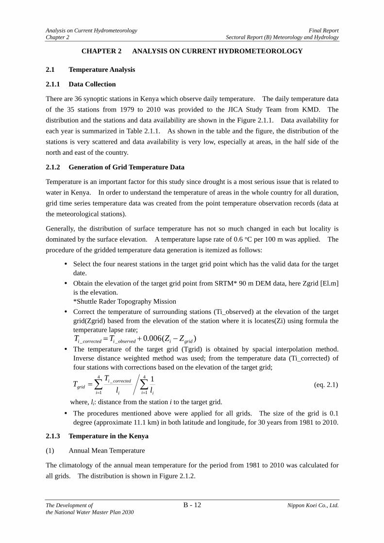
Analysis on Current Hydrometeorology Final Report Chapter 2 Sectoral Report (B) Meteorology and Hydrology
The Development of B - 12 Nippon Koei Co., Ltd. the National Water Master Plan 2030
CHAPTER 2 ANALYSIS ON CURRENT HYDROMETEOROLOGY
2.1 Temperature Analysis
2.1.1 Data Collection
There are 36 synoptic stations in Kenya which observe daily temperature. The daily temperature data of the 35 stations from 1979 to 2010 was provided to the JICA Study Team from KMD. The distribution and the stations and data availability are shown in the Figure 2.1.1. Data availability for each year is summarized in Table 2.1.1. As shown in the table and the figure, the distribution of the stations is very scattered and data availability is very low, especially at areas, in the half side of the north and east of the country.
2.1.2 Generation of Grid Temperature Data
Temperature is an important factor for this study since drought is a most serious issue that is related to water in Kenya. In order to understand the temperature of areas in the whole country for all duration, grid time series temperature data was created from the point temperature observation records (data at the meteorological stations).
Generally, the distribution of surface temperature has not so much changed in each but locality is dominated by the surface elevation. A temperature lapse rate of 0.6 °C per 100 m was applied. The procedure of the gridded temperature data generation is itemized as follows:
Select the four nearest stations in the target grid point which has the valid data for the target date.
Obtain the elevation of the target grid point from SRTM* 90 m DEM data, here Zgrid [El.m] is the elevation. *Shuttle Rader Topography Mission
Correct the temperature of surrounding stations (Ti_observed) at the elevation of the target grid(Zgrid) based from the elevation of the station where it is locates(Zi) using formula the temperature lapse rate;
)(006.0__ gridiobservedicorrectedi ZZTT The temperature of the target grid (Tgrid) is obtained by spacial interpolation method.
Inverse distance weighted method was used; from the temperature data (Ti_corrected) of four stations with corrections based on the elevation of the target grid;
4
1
4
1
_ 1i ii i
correctedigrid ll
TT
(eq. 2.1)
where, li: distance from the station i to the target grid. The procedures mentioned above were applied for all grids. The size of the grid is 0.1
degree (approximate 11.1 km) in both latitude and longitude, for 30 years from 1981 to 2010.
2.1.3 Temperature in the Kenya
(1) Annual Mean Temperature
The climatology of the annual mean temperature for the period from 1981 to 2010 was calculated for all grids. The distribution is shown in Figure 2.1.2.

Final Report Analysis on Current Hydrometeorology Sectoral Report (B) Meteorology and Hydrology Chapter 2
Nippon Koei Co., Ltd. B - 13 The Development of the National Water Master Plan 2030
The eastern side of the country is hot with an annual mean temperature of around 30oC. The high land area in the centre of the country, which around Mt. Kenya, is cool with an annual mean temperature of less than 10 oC. The western side of Mt. Kenya to Lake Victoria has moderate annual mean temperature from 15 oC to 20 oC. The distribution of temperature in the country does not vary all year around.
(2) Seasonal Temperature
The climatology of the mean temperatures of Kenya’s four seasons, namely December – January – February (DJF), March – April – May (MAM), June – July – August (JJA) and September – October – November (SON), were calculated from 1981 to 2010. The charts are shown in Figure 2.1.3.
The climatology of monthly mean temperatures were also calculated for the same period and the charts are shown in Figure 2.1.4.
The distribution of temperature does not vary all year round. Area with cool temperature, which are indicated as green zone in the charts, are smallest in June and largest in February.
2.2 Rainfall Analysis
2.2.1 Data Collection
There were approximately 2000 rainfall stations in Kenya in 1977, of which, collected data from these stations are stored in KMD. The number of rainfall stations has drastically dropped to 1653 by 1988 and to 1497 by 1990. At present, there are only 700 operating rainfall stations left in Kenya.
Data availability from 1981 to 2010 and spatial distribution of the stations were considered for selection of the rainfall stations for this study. The number of stations density is very low in the northern and eastern areas of the country. On the other hand, there are a number of stations in the central and western areas. Therefore, all stations in the northern and eastern areas were selected, even the stations with poor data availability were selected in order to cover the whole nation. Meanwhile, the stations which have good data availability were selected from density area.
The daily rainfall data from 120 stations were obtained from stations KMD database. The distribution of rainfall stations and their data availability are shown in Figure 2.2.1 and Table 2.1.2.
Each rainfall gauging station has a seven digit registration code given by KMD. The first two digits indicate the north polar distance of the latitude circle forming the northern edge of the degree square in which the station is located. The subsequent two digits indicate the meridian of longitude forming the western edge of the degree square. The last three digits are set in ascending order corresponding to the established date of the station.
2.2.2 Generation of Grid Rainfall Data
Grid rainfall data with 0.1 degrees in both latitude and longitude was generated from the point rainfall data (observed data at rainfall gauging station). Inverse distance weighted interpolation was applied where the weight factor of averaging is equal to the inverse of distance (linear). The rainfall data from the nearest four stations which have valid data for the target date were used for interpolation. The grid rainfall data was estimated by the equation below:

Analysis on Current Hydrometeorology Final Report Chapter 2 Sectoral Report (B) Meteorology and Hydrology
The Development of B - 14 Nippon Koei Co., Ltd. the National Water Master Plan 2030
4
1
4
1
1i ii i
i
ll
rr (eq. 2.2)
where, r = grid rainfall (mm) ri= observed daily rainfall at rainfall station i (mm) li= distance between rainfall station i and grid rainfall (km)
The reasons why the grid data is generated for this study are as follows:
To fulfil the missing data. To produce data for areas with no rainfall stations To find out the unreliable stations. (fortunately, there are no stations which can be
recognized as unreliable) To compare with general circulation models (GCMs) which are grid data.
Reliability of the observed data taken by each station was checked with the grid rainfall produced. Any unreliable data obtained were excluded.
2.2.3 Annual Rainfall
The climatology of annual rainfall for the period from 1981 to 2010 is illustrated in Figure 2.2.2. The rainfall of the arid area of the northern half of the country is less than 500 mm per year. The central area around Mt. Kenya, also called the water tower, has over 1,000 mm per year. The western area around Lake Victoria is a humid region. The annual rainfall is over 1,000 mm/year. The coastal area also has much rainfall.
2.2.4 Seasonal and Monthly Rainfall
The climatology of seasonal rainfall for the period from 1981 to 2010 is shown in Figure 2.2.3 and the monthly mean rainfall is shown in Figure 2.2.4.
In Kenya, there are two rainy seasons, namely the short rainy season in November and the long rainy season that usually lasts from the end of March to May. The dry season lasts from June to September.
In western Kenya, especially the Lake Victoria North and South regions, there is no distinctive dry season throughout the year. The maximum rainfall usually occurs in April and November. The double rainy seasons in April and November are well marked in the central Kenya, while the coastal area has a single rainy season in May.
Four stations which have valid data and are nearest to the target grid were used

Final Report Analysis on Current Hydrometeorology Sectoral Report (B) Meteorology and Hydrology Chapter 2
Nippon Koei Co., Ltd. B - 15 The Development of the National Water Master Plan 2030
2.2.5 Frequency Analysis
The three probability density functions (PDFs) listed below are often used in Kenya for rainfall frequency analysis:
Gumbel Distribution (Double Exponential Distribution) Log Normal Distribution Log Pearson III Distribution
Since rainfall distribution varies by areas, the best fitted PDF also differs according to area. Although the best fitted PDF should be applied for frequency analysis, it is important to select the PDF that has consistency of results.
In order to choose the best fitted PDF, the frequency analysis by said three functions was carried out for one, three, and five-day rainfall of the whole of Kenya. Standard least-squares criterion (SLSC) was used to assess the fitness of the result. A smaller value of the SLSC means the better fitness of the sampled rainfall data. The estimation of the parameters of these three PFDs was computed for all grid data and, then the values were summarized by spatial average. As a result, among the three PDFs, the Log Normal Distribution was chosen.
The results of the comparison of the PDFs are shown below.
Source: JICA Study Team with original data provided by KMD
SLSC Value for Comparison of Appropriate Probable Density Function for Whole Kenya
Rainfall frequency analysis (RFA) was conducted for all grids with log-normal distribution. The result of RFA for the major rainfall stations are tabulated below. The results of RFA for the major stations with three PDFs were plotted on the Log Normal probability paper as shown in Figure 2.2.5. Log-normal distribution has the best fitted among three PDFs on most of the stations.
The distribution of the probable rainfall intensity estimated by log-normal distribution is shown in Figures 2.2.6-8. The highland area around Mt. Kenya and the coastal area are relatively higher than other areas.
0.044
0.033 0.036
0.040
0.033 0.035 0.039
0.032 0.034
0.000
0.010
0.020
0.030
0.040
0.050
Gumbel Distribution
Log Normal Distribution
Log Pearson III Distribution
Gumbel Distribution
Log Normal Distribution
Log Pearson III Distribution
Gumbel Distribution
Log Normal Distribution
Log Pearson III Distribution
1 Day 3 Day 5 Day

Analysis on Current Hydrometeorology Final Report Chapter 2 Sectoral Report (B) Meteorology and Hydrology
The Development of B - 16 Nippon Koei Co., Ltd. the National Water Master Plan 2030
Rainfall Frequency Analysis with Log Normal Distribution ( Unit: Daily Rainfall [mm/day] )
p (Non-exceedance Probability) 0.5 0.8 0.9 0.95 0.98 0.99 0.995T (Return Period [years]) 2 5 10 20 50 100 200Monbasa 84.0 119.6 146.6 174.9 214.9 247.5 282.3 Narok 43.6 56.3 64.6 72.4 82.4 89.9 97.4 Nyeri 44.8 60.0 70.9 82.0 97.2 109.2 121.7 Garissa 54.1 79.8 96.5 112.2 132.5 147.6 162.7 Kisumu 56.3 66.2 73.0 79.6 88.4 95.1 102.0 Kitale 43.2 51.1 55.4 59.1 63.4 66.3 69.1 Wajir 47.4 72.8 91.5 110.7 137.5 159.0 181.8 Marsabit 81.4 114.1 132.7 149.0 168.2 181.7 194.4 Lodwar 29.5 44.1 54.5 64.9 79.0 90.1 101.7 Moyale 57.9 81.7 98.5 115.4 138.4 156.4 175.1
Source: JICA Study Team with original data provided by KMD
2.2.6 Number of Rainy Days in a Year
The numbers of rainy days were counted for every grid. The days with rainfall of more than 1mm/day were counted as rainy days. The annual rainy days is shown in Figure 2.2.9.
The western area around Lake Victoria shows a high number of rainy days. The northern area has rainy days of less than 60 to 70 days in a year.
The seasonal climatology numbers of rainy days are shown in the Figure 2.2.10. According to the figure, the seasonal difference of the number of rainy days is recognized.
2.2.7 Annual Rainfall of Drought Year
The drought years with ten-year return period (1/10 drought year) were obtained using the following procedures:
Compute spatial average of annual rainfall in Kenya for 20 years from 1981 to 2000. Sort the annual average rainfall in descending order. The second driest year is extracted as the 1/10 drought year.
The distribution of annual rainfall is shown in Figure 2.2.11. The seasonal drought rainfall is obtained by comparing the mean rainfall of each season. The distributions of the seasonal rainfall are shown in Figure 2.2.12. The extraction of the drought year is done by comparing the data for seasonal rainfall. Therefore, the selected year is different from other seasons as a result.
The distribution of rainfall in the drought year is obviously less than the climatology of annual rainfall. Especially, during the dry season (DJF), rainfall is mainly 1mm/day.

Final Report Trend Analysis of Meteorological Data Sectoral Report (B) Meteorology and Hydrology Chapter 3
Nippon Koei Co., Ltd. B - 17 The Development of the National Water Master Plan 2030
CHAPTER 3 TREND ANALYSIS OF METEOROLOGICAL DATA
3.1 Trend Analysis with Observed Data
The climate trend using actual observed data was carried out to understand how the climate has changed in Kenya for the past half century. The future climate change is however difficult to project from the past trend since it is known that the climate has been changing rapidly due to complex factors such as variations in solar radiation, deviations in the Earth's orbit, and amount of greenhouse gas emissions.
3.2 Available Data
(1) Temperature
1) Synoptic Stations
There are 36 ‘synoptic stations’ which observe several meteorological elements. For the trend analysis of temperature, 14 stations which had been established in the early 1900s were selected considering spatial distribution. The selected stations are listed in Table 3.2.1, and the locations of the selected stations are shown in Figure 3.2.1.
2) Data Collection
The daily maximum and minimum temperatures were collected from the KMD database. The availability of temperature data is shown in Figure 3.2.2. The availability was checked using daily mean temperature which was calculated by averaging the daily maximum and minimum temperature and daily minimum temperatures.
Temperature data is available for only 30 years at most of the stations. Considering the established year of the selected stations, more temperature data seems to be available from other sources, i.e. meteorological data book or database of Ministry of Water and Irrigation (MWI).
(2) Rainfall
1) Synoptic Stations
14 synoptic stations were selected for temperature trend analysis. The 14 stations were also used for rainfall trend analysis.
2) Supplemental Stations
Especially in rainfall analysis, station density is important. Around the Lake Victoria, a few stations are included in the 14 selected stations mentioned before. In NWMP (1992), the 22 stations established in the early 1900s were used for evaluation of long term variation of the annual rainfall depth. Therefore, three of the 22 stations were selected to supplement the spatial distribution. The 17 selected stations are listed in Table 3.2.2, and their locations are shown in Figure 3.2.1.

Trend Analysis of Meteorological Data Final Report Chapter 3 Sectoral Report (B) Meteorology and Hydrology
The Development of B - 18 Nippon Koei Co., Ltd. the National Water Master Plan 2030
3) Data Collection
Daily rainfall data was collected from the database of KMD. Availability of rainfall data is shown in Figure 3.2.3. There are seven stations among the 17 selected stations with observation periods of more than 50 years. Considering the year of establishment of the selected stations, the more data seems to be available in other sources, i.e. meteorological data book or database of MWI.
3.3 Trend Analysis of Temperature
The monthly mean temperature was calculated by averaging the monthly mean maximum and minimum temperature. The annual mean temperature was generated from monthly mean temperature. The annual data with availability of lower than 80% were neglected.
For each item, a five-year moving average calculation and temperature trend analysis were carried out.
T-test was conducted to test the significance of the trend, with the level of significance at 5%. The test statistic T follows a Student-t distribution with n-2 degrees of freedom under the null hypothesis.
Results of the trend analysis of temperature are shown in Figure 3.3.1. The increasing trend is seen in the whole country for annual temperature. The increase of annual mean temperature varies from 0.1 to 0.5 oC per two decades in the Southern Lowland and South Eastern Lowland. In other area, nearly 1.0 oC of two decades in North Western Kenya, Highland West of the Rift Valley and the Central Rift Valley.
Anomaly of annual the annual mean temperature increase per mean temperature is shown below. A linear increasing trend is seen for the recent 50 years.
Note: The baseline was set at the mean temperature of 1980. Source: JICA Study Team
Anomaly of Annual Mean Temperature
3.4 Trend Analysis of Rainfall
Annual rainfall and seasonal rainfall were estimated as the total of the daily rainfall for taht specific periods. The numbers of rainy days were counted from the daily rainfall data. The annual maximum daily rainfall was extracted as the maximum value of the daily rainfall. For seasonal rainfall, the following four seasons were taken into account.
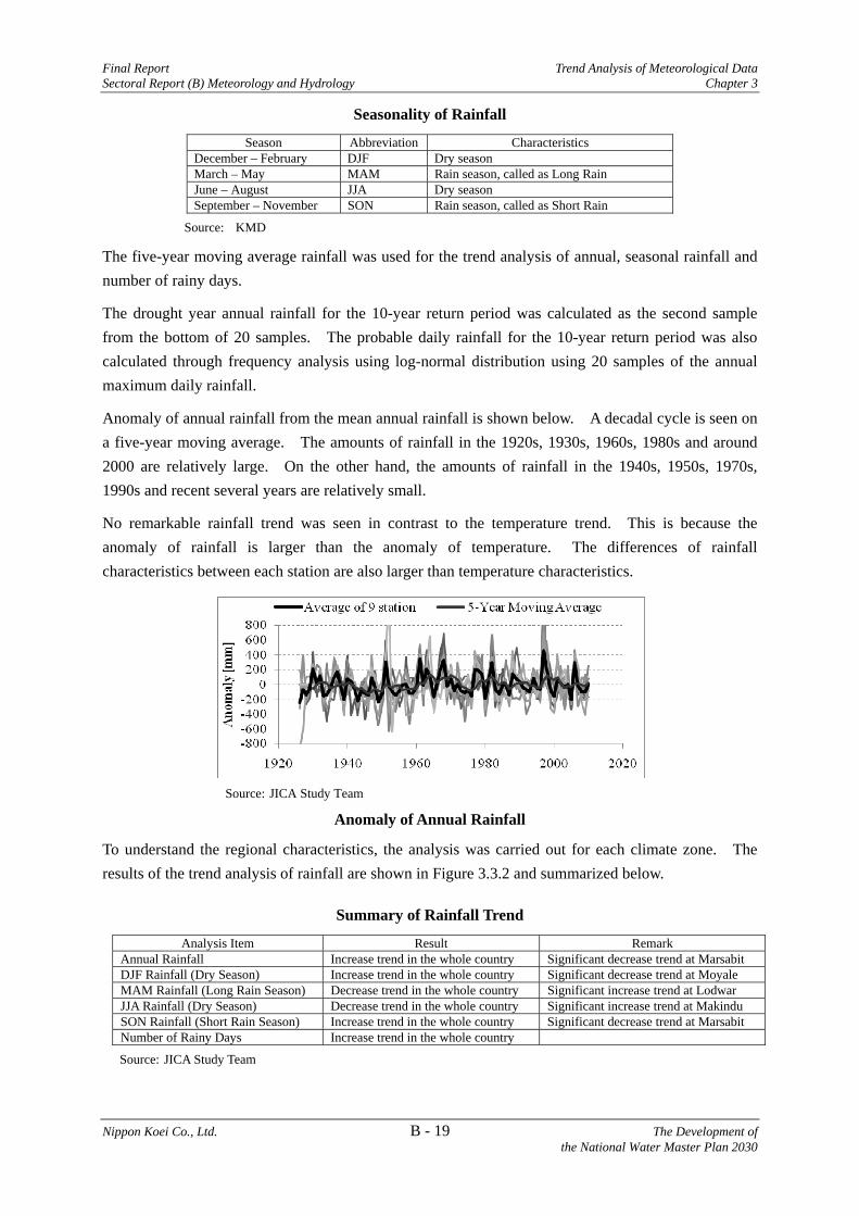
Final Report Trend Analysis of Meteorological Data Sectoral Report (B) Meteorology and Hydrology Chapter 3
Nippon Koei Co., Ltd. B - 19 The Development of the National Water Master Plan 2030
Seasonality of Rainfall
Season Abbreviation Characteristics December – February DJF Dry season March – May MAM Rain season, called as Long Rain June – August JJA Dry season September – November SON Rain season, called as Short Rain
Source: KMD
The five-year moving average rainfall was used for the trend analysis of annual, seasonal rainfall and number of rainy days.
The drought year annual rainfall for the 10-year return period was calculated as the second sample from the bottom of 20 samples. The probable daily rainfall for the 10-year return period was also calculated through frequency analysis using log-normal distribution using 20 samples of the annual maximum daily rainfall.
Anomaly of annual rainfall from the mean annual rainfall is shown below. A decadal cycle is seen on a five-year moving average. The amounts of rainfall in the 1920s, 1930s, 1960s, 1980s and around 2000 are relatively large. On the other hand, the amounts of rainfall in the 1940s, 1950s, 1970s, 1990s and recent several years are relatively small.
No remarkable rainfall trend was seen in contrast to the temperature trend. This is because the anomaly of rainfall is larger than the anomaly of temperature. The differences of rainfall characteristics between each station are also larger than temperature characteristics.
Source: JICA Study Team
Anomaly of Annual Rainfall
To understand the regional characteristics, the analysis was carried out for each climate zone. The results of the trend analysis of rainfall are shown in Figure 3.3.2 and summarized below.
Summary of Rainfall Trend
Analysis Item Result Remark Annual Rainfall Increase trend in the whole country Significant decrease trend at Marsabit DJF Rainfall (Dry Season) Increase trend in the whole country Significant decrease trend at Moyale MAM Rainfall (Long Rain Season) Decrease trend in the whole country Significant increase trend at Lodwar JJA Rainfall (Dry Season) Decrease trend in the whole country Significant increase trend at Makindu SON Rainfall (Short Rain Season) Increase trend in the whole country Significant decrease trend at Marsabit Number of Rainy Days Increase trend in the whole country
Source: JICA Study Team

Trend Analysis of Meteorological Data Final Report Chapter 3 Sectoral Report (B) Meteorology and Hydrology
The Development of B - 20 Nippon Koei Co., Ltd. the National Water Master Plan 2030
The anomaly of the annual number of rainy days from the mean annual number of rainy days is shown below. A cycle of about the hundred years is seen for the number of rainfall days. The number of rainy days has been decreasing from around 1980 to the present years following the cycle.
Source: JICA Study Team
Anomaly of Number of Rainy Days

Final Report Climate Change Analysis Sectoral Report (B) Meteorology and Hydrology Chapter 4
Nippon Koei Co., Ltd. B - 21 The Development of the National Water Master Plan 2030
CHAPTER 4 CLIMATE CHANGE ANALYSIS
4.1 Approach to the Analysis
Weather is varied widely every day, every month and every year. Climate is the long-term, average behaviour of weather for a particular region, which is usually considered to be stable. Based on the concept that the climate is stable, hydrological studies have been conducted, and planned values, such as rainfall intensity, have been established through statistical study from observed past records.
Climate is changing naturally. The rate of change has accelerated significantly due to human activities. The target year of this master plan is 2030. Though it is only for a period of 20 years, it may be difficult to consider that future climate conditions will be the same as current conditions. In order to understand the future hydrological condition for development of the master plan, climate change may not be neglected. The impact of climate change on Kenya was evaluated in this study.
A general circulation model (GCM) is the most hopeful and advanced tool to understand the climate and to project future climate conditions. Many GCMs have been developed in various countries. It was first introduced in the country dudring the Fourth Assessment Report (AR4) conducted by the Intergovernmental Panel on Climate Change (IPCC). Most of those data are archived in the Phase 3 of the Coupled Model Intercomparison Project (CMIP3). In this study, climate change in Kenya was studied using the results of the GCMs.
Although the GCMs are accepted widely as the best physically based tool for devising climate scenarios, there is a considerable gap between local climate conditions and simulation results. These gaps are called bias. In order to apply the GCMs results to the catchment scale, bias corrections were made based on the methodology propounded by Professor Koike of the University of Tokyo.
There are 17 GCMs that are available in the daily data sets. The daily data sets of GCMs are archived in the Data Integration and Analysis System (DIAS) Japan as well as CMIP3. The daily data sets were provided to JICA from DIAS as a part of the cooperation between the University of Tokyo’s Earth Observation Data Integration and Fusion Research Initiative (EDITORIA) and JICA.
Every GCM has a future scenario which is different from other GCMs. Even GCMs, equipped with state-of-the-arts of technology, can not project an assured future climate. This uncertainty of the future climate should be evaluated quantitatively. Multi model ensemble analysis was carried out to evaluate the uncertainty of future climate. Such uncertainty should be taken into account in developing NWMP 2030.
The flowchart of climate change analysis is shown below.
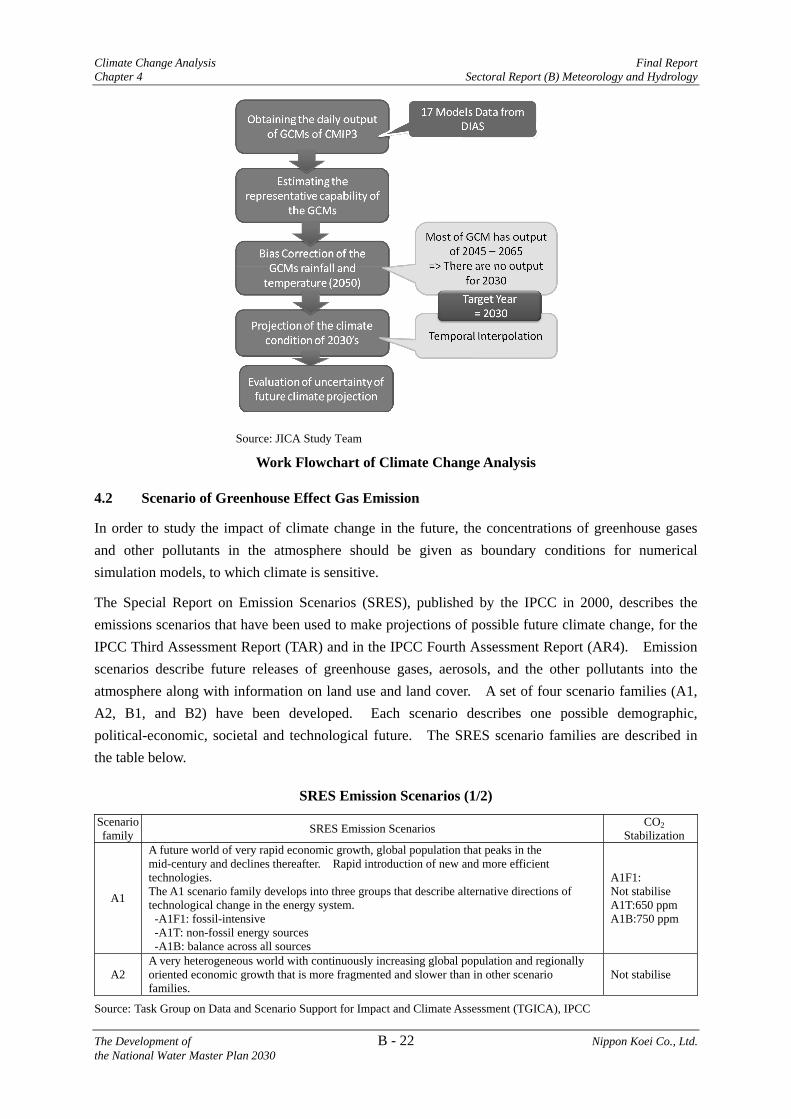
Climate Change Analysis Final Report Chapter 4 Sectoral Report (B) Meteorology and Hydrology
The Development of B - 22 Nippon Koei Co., Ltd. the National Water Master Plan 2030
Source: JICA Study Team
Work Flowchart of Climate Change Analysis
4.2 Scenario of Greenhouse Effect Gas Emission
In order to study the impact of climate change in the future, the concentrations of greenhouse gases and other pollutants in the atmosphere should be given as boundary conditions for numerical simulation models, to which climate is sensitive.
The Special Report on Emission Scenarios (SRES), published by the IPCC in 2000, describes the emissions scenarios that have been used to make projections of possible future climate change, for the IPCC Third Assessment Report (TAR) and in the IPCC Fourth Assessment Report (AR4). Emission scenarios describe future releases of greenhouse gases, aerosols, and the other pollutants into the atmosphere along with information on land use and land cover. A set of four scenario families (A1, A2, B1, and B2) have been developed. Each scenario describes one possible demographic, political-economic, societal and technological future. The SRES scenario families are described in the table below.
SRES Emission Scenarios (1/2)
Scenario family SRES Emission Scenarios CO2
Stabilization
A1
A future world of very rapid economic growth, global population that peaks in the mid-century and declines thereafter. Rapid introduction of new and more efficient technologies. The A1 scenario family develops into three groups that describe alternative directions of technological change in the energy system. -A1F1: fossil-intensive -A1T: non-fossil energy sources -A1B: balance across all sources
A1F1: Not stabilise A1T:650 ppm A1B:750 ppm
A2 A very heterogeneous world with continuously increasing global population and regionally oriented economic growth that is more fragmented and slower than in other scenario families.
Not stabilise
Source: Task Group on Data and Scenario Support for Impact and Climate Assessment (TGICA), IPCC
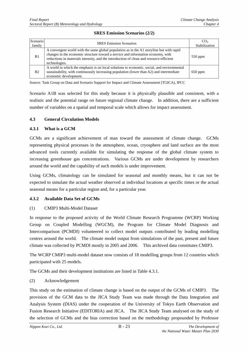
Final Report Climate Change Analysis Sectoral Report (B) Meteorology and Hydrology Chapter 4
Nippon Koei Co., Ltd. B - 23 The Development of the National Water Master Plan 2030
SRES Emission Scenarios (2/2)
Scenario family SRES Emission Scenarios CO2
Stabilization
B1
A convergent world with the same global population as in the A1 storyline but with rapid changes in the economic structure toward a service and information economy, with reductions in materials intensity, and the introduction of clean and resource-efficient technologies.
550 ppm
B2 A world in which the emphasis is on local solutions to economic, social, and environmental sustainability, with continuously increasing population (lower than A2) and intermediate economic development.
650 ppm
Source: Task Group on Data and Scenario Support for Impact and Climate Assessment (TGICA), IPCC
Scenario A1B was selected for this study because it is physically plausible and consistent, with a realistic and the potential range on future regional climate change. In addition, there are a sufficient number of variables on a spatial and temporal scale which allows for impact assessment.
4.3 General Circulation Models
4.3.1 What is a GCM
GCMs are a significant achievement of man toward the assessment of climate change. GCMs representing physical processes in the atmosphere, ocean, cryosphere and land surface are the most advanced tools currently available for simulating the response of the global climate system to increasing greenhouse gas concentrations. Various GCMs are under development by researchers around the world and the capability of such models is under improvement.
Using GCMs, climatology can be simulated for seasonal and monthly means, but it can not be expected to simulate the actual weather observed at individual locations at specific times or the actual seasonal means for a particular region and, for a particular year.
4.3.2 Available Data Set of GCMs
(1) CMIP3 Multi-Model Dataset
In response to the proposed activity of the World Climate Research Programme (WCRP) Working Group on Coupled Modelling (WGCM), the Program for Climate Model Diagnosis and Intercomparison (PCMDI) volunteered to collect model outputs contributed by leading modelling centres around the world. The climate model output from simulations of the past, present and future climate was collected by PCMDI mostly in 2005 and 2006. This archived data constitutes CMIP3.
The WCRP CMIP3 multi-model dataset now consists of 18 modelling groups from 12 countries which participated with 25 models.
The GCMs and their development institutions are listed in Table 4.3.1.
(2) Acknowledgement
This study on the estimation of climate change is based on the output of the GCMs of CMIP3. The provision of the GCM data to the JICA Study Team was made through the Data Integration and Analysis System (DIAS) under the cooperation of the University of Tokyo Earth Observation and Fusion Research Initiative (EDITORIA) and JICA. The JICA Study Team analysed on the study of the selection of GCMs and the bias correction based on the methodology propounded by Professor

Climate Change Analysis Final Report Chapter 4 Sectoral Report (B) Meteorology and Hydrology
The Development of B - 24 Nippon Koei Co., Ltd. the National Water Master Plan 2030
Koike of the University of Tokyo who is the leading academic for the study in the field of climate change adaptation and promoting the project of DIAS.
The JICA Study Team also acknowledges the modelling groups, the Program for Climate Model Diagnosis and Intercomparison (PCMDI) and the WCRP's Working Group on Coupled Modelling (WGCM) for their roles to make the WCRP CMIP3 multi-model dataset available. Support of this dataset was provided by the Office of Science of the U.S. Department of Energy.
4.4 Selection of General Circulation Models
4.4.1 General
The results of the GCMs have very large diversity, and the diversity can be translated into the uncertainty of the projection of future climate. However, the models with significantly low reproducibility of the current climate conditions should not be considered deselected from the consideration. The reproducibility of GCMs was evaluated by comparing of the climatology of observed climate data and the simulation result of run for the reproduction of the current climate conditions. These simulation cases are called “20c3m” scenario. The observed and the simulated climatology cover the period from 1981 to 2000.
The evaluation of the reproducibility of the GCMs is based on the methodology propounded by Professor Koike of the University of Tokyo.
4.4.2 Methodology of the Selection
The reproducibility of the GCMs was evaluated through the following procedures.
1) The gridded observed data for four variables of climate were obtained from the web site of the National Oceanic and Atmospheric Administration (NOAA). The gridded data were produced based on the observed data and mathematical atmospheric simulation model. The data is called “reanalysis data”. Four variables were chosen as they are considered main climate elements to represent the regional climate conditions. The collected reanalysis data are listed in the table below.

Final Report Climate Change Analysis Sectoral Report (B) Meteorology and Hydrology Chapter 4
Nippon Koei Co., Ltd. B - 25 The Development of the National Water Master Plan 2030
Collected Reanalysis Data
Variable Standard Name Notes
pr Precipitation
Global Precipitation Climatology Project (GPCP) Version 2.2 Climatology Precipitation Acknowledgement: The GPCP combined precipitation data were developed and computed; the NASA/Goddard Space Flight Center's Laboratory for Atmospheres as a contribution to the GEWEX Global Precipitation Climatology Project. from their Web site at http://www.ncdc.noaa.gov/oa/
olr
Outgoing Longwave Radiation (OLR)
20 years(1981-2000) Climatology of OLR from interpolated OLR dataset Created from monthly means of OLR from National Oceanic Atmospheric Administration (NOAA) Acknowledgement: Interpolated OLR data provided by the NOAA/OAR/ESRL PSD, Boulder, Colorado, USA, from their Web site at http://www.esrl.noaa.gov/psd/
slp Sea Level Pressure
20 years(1981-2000) Climatology of Sea Level Pressure Created from National Centers for Environmental Prediction (NCEP) Reanalysis monthly Sea Level Pressure Acknowledgement: NCEP Reanalysis Derived data provided by the NOAA/OAR/ESRL PSD, Boulder, Colorado, USA, from their Web site at http://www.esrl.noaa.gov/psd/
tas Surface Air Temperature
20 years(1981-2000) Climatology of air temperature Created from NCEP Reanalysis monthly air temperature Acknowledgement: NCEP Reanalysis Derived data provided by the NOAA/OAR/ESRL PSD, Boulder, Colorado, USA, from their Web site at http://www.esrl.noaa.gov/psd/
Source: JICA Study Team
2) The climatology of monthly mean values of the gridded observed data from 1981 to 2000 were calculated.
3) There are 17 GCMs taht were selected as the daily monthly data are available in the CMIP3 and DIAS, though there are 25 models. The monthly data of the 20c3m experiments of the period from 1981 to 2000 were obtained. The data availability of the GCMs is summarized in Table 4.4.1. There are 17 models collected for this study which are numbered in the table.
4) The climatology of the monthly mean values of the GCMs were calculated for all variables. 5) The correlation factor and root mean square error (RMSE) were applied for comparison. 6) Both the observed data and GCM data are re-gridded into 0.1 degree grid sizes in both
latitude and longitude. In order to evaluate in a large scale, the range from 10 º South to 10 º North and from 25 º East to 50 º East were considered.
7) The indexes for comparison were calculated for every grid. Finally, the real average of every index was evaluated.
4.4.3 Selection of GCMs
A comparison of monthly mean climatology between the observed data and GCMs data were made. An example of the results of comparison is shown below.

Climate Change Analysis Final Report Chapter 4 Sectoral Report (B) Meteorology and Hydrology
The Development of B - 26 Nippon Koei Co., Ltd. the National Water Master Plan 2030
Source: JICA Study Team with following original data
The GPCP Version 2.2 combined precipitation data, the DIAS dataset, and the CMIP3 multi-model dataset.
Comparison of Monthly Mean Precipitation
The left chart shows the observed precipitation climatology. The middle and right charts show the climatology of GCMs data. The distribution of the rainfall intensity in the middle chart is similar to the observed data. Meanwhile, the distribution pattern and rainfall intensity in the right side model are significantly different from the observed data. The correlation factor and RMSE for each model are indicated in the above chart. The correlation factor of the middle model is 0.88, which is it is close to 1.0. It means the climatology of the GCM in the middle chart is similar to the observed one. Therefore, it can be considered that the indexes of correlation factor and RMSE are applicable for evaluation of the reproducibility of the model.
Four variables for all 17 GCMs for 12 months were evaluated in the same manner. All evaluated indexes were summarized in the form of the chart shown below.
Source: JICA Study Team with following original data The GPCP Version 2.2 combined precipitation data, the DIAS dataset, and the CMIP3
multi-model dataset. Evaluation of the Reproducibility of the GCMs
0.00
0.20
0.40
0.60
0.80
1.00
1.20
Jan Feb Mar Apr May Jun Jul Aug Sep Oct Nov Dec
corr
elat
ion
Precipitation (pr)
giss‐aom
giss_model_e_r

Final Report Climate Change Analysis Sectoral Report (B) Meteorology and Hydrology Chapter 4
Nippon Koei Co., Ltd. B - 27 The Development of the National Water Master Plan 2030
According to the chart above, most of the lines show almost the same capability except for two models, giss_model_e_r and giss_aom. The lines of these two models are different from the others. These models are excluded for the further study, because these two models show poor reproducibility of current climatology of Kenya. The evaluated values of correlation factor and RMSE were shown in the Figure 4.4.1 and the names of the models were shown in the charts which are excluded for the further study because of their poor reproducibility. The evaluated values of correlation factor and RMSE are tabulated from Table 4.4.2 to 4.4.9.
Table 4.4.10 summarises the result of selection of GCMs mentioned above. Six GCMs were excluded. The selected 11 GCMs are; Cccma_cgcm3_1, cccma_cgcm3_1_t63, cnrm_cm3, csiro_mk3_0, gfdl_cm2_0, gfdl_cm2_1, ipsl_cm4, miroc3_2_hires, miroc3_2_medres, mpi_echam5 and mri_cgcm2_3_2a.
4.5 Bias Correction
4.5.1 Necessity of Bias Correction
GCMs are effective tools to project future climate conditions. However, GCMs have a bias in simulating 20th century precipitation and temperature. Therefore, GCMs cannot be used directly on hydrological models in order to assess the impact of the projected climate change for the particular basin. This is the reason why bias correction is necessary.
The well-known problems of the GCMs are as follows:
a) Large diversity of the models b) Low seasonal representation c) Low extreme heavy rainfall rate d) Small number of no rainfall day but long drizzle
In order to solve the problems above, statistical bias correction was conducted.
4.5.2 Methodology of Bias Correction
(1) General
Bias is a gap between the observed data and the output of the GCMs for a certain meteorological index such as annual mean rainfall, monthly mean rainfall, rainfall frequency, etc. Although the output of GCMs have dates as if it is along with the actual calendar, the daily rainfall it cannot be compared with the actual record of the same date. For instance in January 1, 1990 GCM output cannot be compared with the actual January 1, 1990 recorded, because the simulation of 20c3m are implemented by giving only the boundary conditions which is not an actual observed data. Therefore, bias correction is made to adjust the simulated climatology to the observed climatology.
For the output of the future A1B simulation, the relationship of the gap correction obtained from the current climate is supposed to be applicable. The difference of A1B and 20c3m is also applied to the projection of the future climate.
The methodology for bias correction that is applied in this study is based on the idea advocated by Professor Koike of University of Tokyo.

Climate Change Analysis Final Report Chapter 4 Sectoral Report (B) Meteorology and Hydrology
The Development of B - 28 Nippon Koei Co., Ltd. the National Water Master Plan 2030
(2) Points of View for Bias Correction
Bias correction of rainfall is carried out through the following process.
a) Correction to monthly climatology b) Correction of no rainfall days c) Correction of high intensity rainfall
The bias correction corresponds with the problems of the GCMs mentioned above.
(3) Correction to Monthly Climatology
The cumulative distribution function based bias correction method (CDF method) was applied to match the rainfall climatology of 20c3m with the observed. Then the relationship of the bias and the 20c3m data is applied to the A1B data. The CDF method is called as sorting method. The procedure for bias correction is as follows;
i) The GCMs grid data were re-gridded into the same grid dimension with the gridded observed rainfall data, provided in this study. The grid size is 0.1 degree in both of latitude and longitude directions.
ii) The monthly mean rainfall of the observed and 20c3m are computed for the period from 1981 to 2000.
iii) All daily rainfall data of a certain month are extracted and sorted in descending order. For example, the daily rainfall in April for 20 years is counted as 600. The figure below shows a schematic image of this extraction and sorting work.
Source: JICA Study Team
Schematic Image of Extraction and Sorting for Daily Rainfall of a Certain Month
iv) For a certain rank of rainfall of 20c3m, the bias is considered as the gap between 20c3m and the observed data with the same rank.
v) Rainfall with a certain rank of 20c3m was replaced by that with the same rank of the observed data. Therefore, the bias-corrected climatology of the monthly mean rainfall of 20c3m is to be completely matched with the observed. This procedure is illustrated in the figure below.
Extracting all rainfall data in a certain month.
Sorting all extracted data in descending order. The sorted rank can be considered as the non-exceedance probability.
Time series of the daily rainfall for 20 years

Final Report Climate Change Analysis Sectoral Report (B) Meteorology and Hydrology Chapter 4
Nippon Koei Co., Ltd. B - 29 The Development of the National Water Master Plan 2030
Source: JICA Study Team
Schematic Image of Bias Correction Based on Sorted Rank
vi) The daily rainfall of the A1B for 20 years from 2046 to 2065 was processed in the same manner with the observed data and 20c3m.
vii) To correct the bias of the rainfall of a certain rank, the gap between the 20c3m and the observed data of the same rank is added. The procedure is illustrated in the figure below.
Source: JICA Study Team
Schematic Image of Bias Correction for Output of A1B (2046-2065)
Bias correction for temperature was carried out in the same manner mentioned above. Since the temperature does not have eccentric behaviour temporally, the bias correction procedure is appropriate to match the climatology of temperature.
(4) Correction of No Rainfall Days
The number of no rainfall days of GCMs is less than that of the observed data. The comparison of the observed and the output of GCM are shown below.

Climate Change Analysis Final Report Chapter 4 Sectoral Report (B) Meteorology and Hydrology
The Development of B - 30 Nippon Koei Co., Ltd. the National Water Master Plan 2030
Source: JICA Study Team with following original data
Kenya Meteorological Department, the DIAS dataset, and the CMIP3 multi-model dataset.
Tail Part of Sorted Daily Rainfall Data and Bias of No Rainfall Days
The considered duration is 20 years and rainfall for April was extracted and sorted. The rainfall data sets of 600 days were obtained for the observed (gray bar) and simulated. The chart above shows the tail part of the sorted rainfall. The gray coloured area indicates the observed rainfall. This chart is for April having heavy rainfall season in Kenya. Therefore, there are rainfalls around the rank of 500. However, the doted curve, which is sorted for raw rainfall data in the GCMs, indicate that there are rainfalls up to the end of the data. This is a bias of no rainfall days.
The bias correction procedure for no rainfall days is as follows:
i) The rainfall value of 20c3m of the last observed rainfall is made the threshold of no rainfall day.
ii) The rainfall for the A1B scenario that is less than the threshold is corrected as zero.
(5) Correction of High Intensity Rainfall
The GCM rainfall of the GCM has low inflection intensity, but problems can be corrected by using the sorting method mentioned above. If there is a heavy rainfall out-of-the season as simulated in the GCM, the result will be rejected because the observed climatology of the month does not have such heavy rainfall. This is the reason why bias correction for high intensity rainfall is necessary.
To cope with the problems of GCMs, plotting position method was applied. The procedure of the method is as follows:
i) The annual maximum daily rainfalls are extracted from the observed and 20c3m data on a certain grid.
ii) Cunnan plot is applied to estimate the non-exceedance probability of the extracted rainfalls.
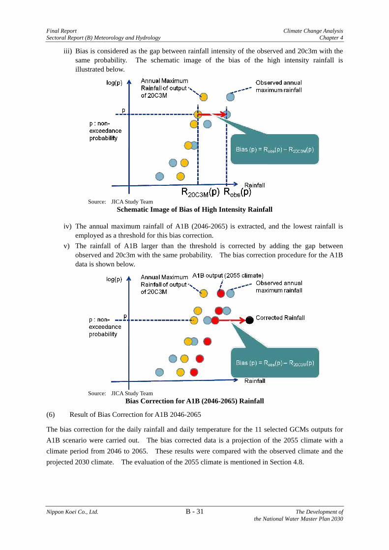
Final Report Climate Change Analysis Sectoral Report (B) Meteorology and Hydrology Chapter 4
Nippon Koei Co., Ltd. B - 31 The Development of the National Water Master Plan 2030
iii) Bias is considered as the gap between rainfall intensity of the observed and 20c3m with the same probability. The schematic image of the bias of the high intensity rainfall is illustrated below.
Source: JICA Study Team
Schematic Image of Bias of High Intensity Rainfall
iv) The annual maximum rainfall of A1B (2046-2065) is extracted, and the lowest rainfall is employed as a threshold for this bias correction.
v) The rainfall of A1B larger than the threshold is corrected by adding the gap between observed and 20c3m with the same probability. The bias correction procedure for the A1B data is shown below.
Source: JICA Study Team
Bias Correction for A1B (2046-2065) Rainfall
(6) Result of Bias Correction for A1B 2046-2065
The bias correction for the daily rainfall and daily temperature for the 11 selected GCMs outputs for A1B scenario were carried out. The bias corrected data is a projection of the 2055 climate with a climate period from 2046 to 2065. These results were compared with the observed climate and the projected 2030 climate. The evaluation of the 2055 climate is mentioned in Section 4.8.

Climate Change Analysis Final Report Chapter 4 Sectoral Report (B) Meteorology and Hydrology
The Development of B - 32 Nippon Koei Co., Ltd. the National Water Master Plan 2030
4.6 Projection of 2030 Climate
4.6.1 Data Availability Representing 2030 Climate
The target year of this NWMP is 2030. The rainfall and temperature data for the period from 2021 to 2040 are needed for the assessment of the impacts of climate change on Kenya. Actually, the simulations of every GCM for the period around 2030 have been implemented, but the daily output was abolished or could not be obtained due to the huge size of the data. The 2030 climate was projected from the observed climate (1990) and bias-corrected A1B 2055 climate.
4.6.2 Methodology of the Projection of 2030 Climate
The methodology of the projection is based on simple temporal interpolation. The monthly mean rainfall and temperature data of GCMs can be obtained from the web site of the IPCC Data Distribution Center (http://www.ipcc-data.org). The projection of 2030 climate was made using the following procedures:
i) The monthly mean climatology of the considered GCMs was computed for the 2030 climate, which has uncorrected bias.
ii) The monthly climatology of 20c3m and A1B 2046-2065 is calculated in the same manner with the 2030 data for GCMs.
iii) The changing ratios of the climatology for every month were evaluated. The changing ratio is evaluated as the ratio of the difference from the 20c3m results between the 2055 climate and the 2030 climate from the 20c3m. The schematic image of this procedure is shown in the figure below.
Source: JICA Study Team
Schematic Image of Projection of 2030 Climate (1)
i) The time-series of the observed grid data is a base time-series for the projection of the rainfall and temperature of the 2030 climate.
ii) Preliminary data for, a certain month of the observed and bias-corrected A1B 2055 data are extracted and sorted.
iii) Rainfall or temperature of the 2030 climate can be projected by applying the changing ratio to the difference between values of the bias-corrected 2055 climate and the observed with the same rank.
iv) The evaluated rainfall or temperature for the 2030 climate is re-sorted along with occurrences of the observed data. The projected time-series of every GCM are based on the same time-series data.
55
30
R
R
mcCli RRR 3205555
mcCli RRR 3203030
20c3m(1981-2000)
2030 2055
Monthly Climatology Data
Changing ratio

Final Report Climate Change Analysis Sectoral Report (B) Meteorology and Hydrology Chapter 4
Nippon Koei Co., Ltd. B - 33 The Development of the National Water Master Plan 2030
The schematic image of the projection of the 2030 climate is shown below.
Source: JICA Study Team
Schematic Image of Projection of 2030 Climate (2)
4.7 Evaluation of Uncertainty of Projected Future Climate
The projected daily rainfall and temperature data of 11 GCMs for the 2030 climate and the 2055 climate are obtained from the foregoing processes. One of the problems of GCMs is that the output from each model widely differ among each other. The diversity will be a natural behaviour. It is important for assessment of future climates to consider the uncertainty of the phenomena.
The simplest summarising method of the diversified future is by the use of ensemble mean. Mean values from future projections can be considered as the most expected future.
There are 11 climate data each for the 2030 and 2055 climates. The number of models is not enough to suppose that the data are distributed on normal distribution. Therefore, the student’s t-distribution was applied for the evaluation of uncertainty. From the evaluation by the t-distribution, the standard deviation and the confidential interval can be obtained for every index.
The example of the evaluation chart of the uncertainty is shown in the figure below.
Source: JICA Study Team
Evaluation Chart of Uncertainty of Future
Cross dots are projected future value of each GCMs
This curve shows student’s t-distribution.
Confidential Intervals are shown

Climate Change Analysis Final Report Chapter 4 Sectoral Report (B) Meteorology and Hydrology
The Development of B - 34 Nippon Koei Co., Ltd. the National Water Master Plan 2030
This is a result of the annual rainfall climatology at Garissa. The year is plotted on the x-axis and the indexed value (annual rainfall) is plotted on the y-axis. The cross dots on the 2030 and 2055 years are the projected GCM values. The distribution of the probability of the mean value is shown as a curve on the 2030 and 2055 year. From the distribution curve, the range of the uncertainty can be acquired using cognizance. The area of the distribution is the probability. The curve is located above the value of the observed. This means that annual rainfall at Garissa will surely increase.
4.8 Evaluation of Projected Future Climate in Kenya
4.8.1 Annual Precipitation
Figure 4.8.1 shows that the annual rainfall will increase over the country. The distribution of the rainfall will not be changed so much. The annual mean precipitation area of the highland area, which is located on the western south part of the country, will increase from 50 to 100 mm/year in the 2030 climate projection, however, it should be noted that the standard deviation of this area is larger than in the other areas. The probability of increase will be sure for the whole country.
4.8.2 Seasonal Precipitation
1) MAM (March – April – May)
MAM is the heavy rainy season in Kenya. Future rainfall of the highland area will increase, but the rainfall at coastal areas will be unchanged or decreased. The result of the ensemble analysis is shown in the Figure 4.8.2.
2) JJA (June – July – August)
JJA is the long dry season in Kenya. The result of the ensemble analysis is shown in Figure 4.8.3. Future seasonal rainfall of JJA will be almost unchanged over the country. The rainfall of coastal area will decrease.
3) SON (September – October – November)
SON is the short rainy season in Kenya. The result of the ensemble analysis for future seasonal rainfall is shown in Figure 4.8.4. Future rainfall for half of the western area including the upper Rift Valley area, which has a semi-arid climate, will increase. The southern area including the coastal area will be unchanged. The increase of rainfall is probable over the country.
4) DJF (December – January – February)
DJF is the short dry season in Kenya. The result of the ensemble analysis for future seasonal rainfall is shown in Figure 4.8.5. Future seasonal rainfall will increase over the country, especially the rainfall of the half of the southern area including the coast area which willm increase significantly.
4.8.3 Rainfall Frequency
The ensemble analyses for the rainfall frequencies of 10, 50 and 100 years return periods were carried out. The results of rainfall frequency analysis are shown in Figures 4.8.6 to the Figure 4.8.8. The

Final Report Climate Change Analysis Sectoral Report (B) Meteorology and Hydrology Chapter 4
Nippon Koei Co., Ltd. B - 35 The Development of the National Water Master Plan 2030
projection for the extreme event rainfall is very difficult. It is important to note that the result is dominated by the methodology. The distributions of rainfall intensity for the future climates in 2030 and 2055 are very similar to that of the current climate. The difference in rainfall intensity for 50-year return period of the future from that of the current is varied by about 50 mm/day less to 50 mm/day more against the current values.
4.8.4 Number of Annual Rainy Days
The days with rainfall larger than 1 mm/day are counted as rainy days. The result of the ensemble analysis over the whole country is shown in Figure 4.8.9. The number of rainy days will increase over the country, especially in the northern area where it will increase significantly. The increase may be almost probable over the country.
4.8.5 Number of Seasonal Wet Days
The results of ensemble analysis for each seasons are shown in Figures 4.8.10 to the Figure 4.8.13.
1) MAM (March – April – May)
The numbers of rainy days will increase or be unchanged. The north Rift Valley area may have significant increase.
2) JJA (June – July – August)
The number of rainy days will increase for most of the country; however, for the coastal area will have slightly decrease in the 2055 climate.
3) SON (September – October – November)
The increase in the number of rainy days in the northern Rift Valley in the 2030 climate and of the southern Rift Valley in the 2055 climate is remarkable.
4) DJF (December – January – February)
Lake Victoria area in the 2030 climate has a high number of rainy days.
4.8.6 Annual Rainfall for the Drought Year in 10-Year Return Period
The evaluation periods for the observed, 2030 and 2055 climate are 20 years. The drought year in the 10-year return period can be obtained as the second driest year of the annual rainfall. This evaluation was done for every grid. The selected year for a certain grid is different from those of the other grids. The evaluated ensemble annual rainfall of the drought year for each grid is shown in Figure 4.8.14.
The rainfall during the drought year will increase in most areas of the country. However, a significant decrease in rainfall for the 2055 climate may happen in coastal areas.
4.8.7 Seasonal Rainfall for the Drought Year in the 10-Year Return Period
The charts of the essential ensemble seasonal rainfall folr the drought year in each grid are shown in Figure 4.8.15 to Figure 4.8.18.
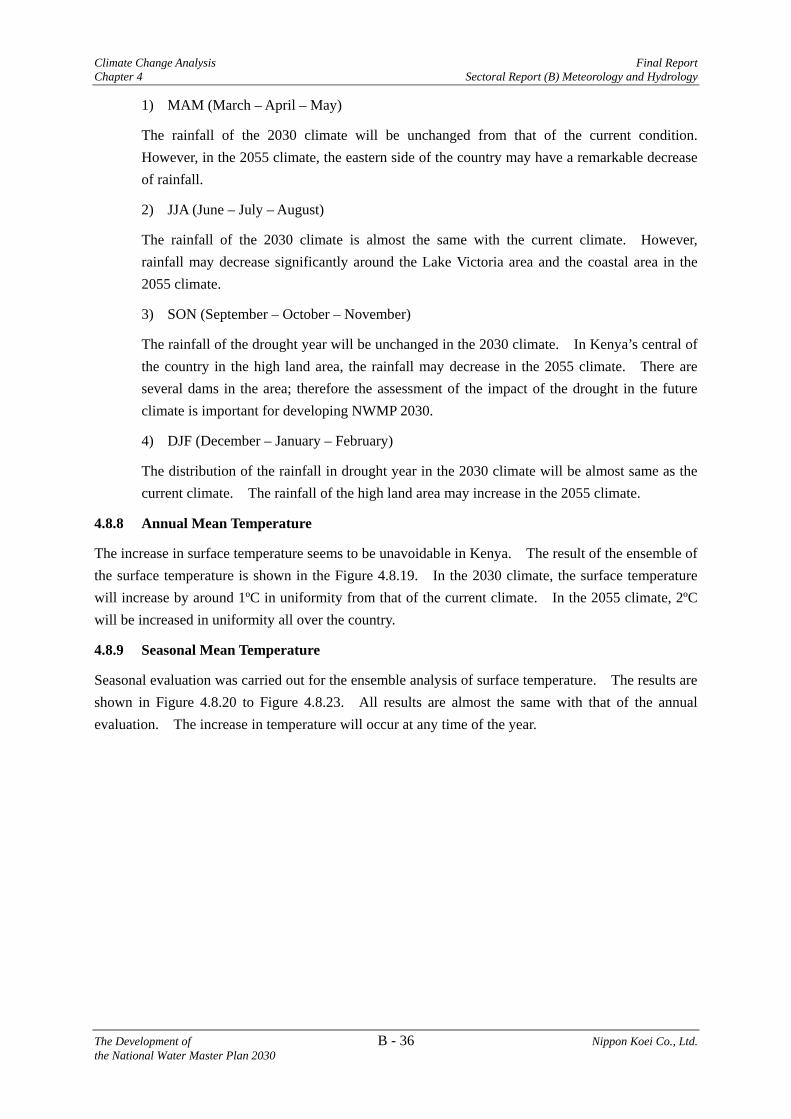
Climate Change Analysis Final Report Chapter 4 Sectoral Report (B) Meteorology and Hydrology
The Development of B - 36 Nippon Koei Co., Ltd. the National Water Master Plan 2030
1) MAM (March – April – May)
The rainfall of the 2030 climate will be unchanged from that of the current condition. However, in the 2055 climate, the eastern side of the country may have a remarkable decrease of rainfall.
2) JJA (June – July – August)
The rainfall of the 2030 climate is almost the same with the current climate. However, rainfall may decrease significantly around the Lake Victoria area and the coastal area in the 2055 climate.
3) SON (September – October – November)
The rainfall of the drought year will be unchanged in the 2030 climate. In Kenya’s central of the country in the high land area, the rainfall may decrease in the 2055 climate. There are several dams in the area; therefore the assessment of the impact of the drought in the future climate is important for developing NWMP 2030.
4) DJF (December – January – February)
The distribution of the rainfall in drought year in the 2030 climate will be almost same as the current climate. The rainfall of the high land area may increase in the 2055 climate.
4.8.8 Annual Mean Temperature
The increase in surface temperature seems to be unavoidable in Kenya. The result of the ensemble of the surface temperature is shown in the Figure 4.8.19. In the 2030 climate, the surface temperature will increase by around 1ºC in uniformity from that of the current climate. In the 2055 climate, 2ºC will be increased in uniformity all over the country.
4.8.9 Seasonal Mean Temperature
Seasonal evaluation was carried out for the ensemble analysis of surface temperature. The results are shown in Figure 4.8.20 to Figure 4.8.23. All results are almost the same with that of the annual evaluation. The increase in temperature will occur at any time of the year.

Final Report Climate Change Analysis Sectoral Report (B) Meteorology and Hydrology Chapter 4
Nippon Koei Co., Ltd. B - 37 The Development of the National Water Master Plan 2030
4.9 Climate Change Impact on Kenya
4.9.1 Estimation of Potential Evapotranspiration
(1) Equations for Evapotranspiration Estimation
Evapotranspiration is the sum of evaporation and transpiration. This phenomenon appear to vary widely depending on weather conditions such as temperature, humidity, sunshine hours and intensity, precipitation, soil type, soil saturation, wind, and land slope. The evaluation of evapotranspiration is difficult because it cannot be measured directly. The several equations for the evaluation of evapotranspiration were proposed. The equations can be classified into 2 types; one is an empirical equations and another is a physical based equations.
The empirical type needs only one or two observed parameters and most of this type equation requires air temperature and sunshine duration on site. The most of the empirical type equation was developed through regression analysis and those are based on the assumption that the parameter is correlated highly and dominantly with evapotranspiration.
Meanwhile, the physical based equations require many types of observed parameters. For instance, FAO Penman-Monteith method requires air temperature, daily solar radiation, wind speed, atmospheric pressure and actual vapour pressure. The physical based equation derives reliable evapotranspiration evaluation for anywhere and any seasons, if the sufficient observed parameter is obtained. In other words, the physical based equation is limited for application, since it is difficult to obtain sufficient parameters.
(2) Estimation of Present and Future Potential Evapotranspiration
Daily air temperature data for 35 stations from 1979 to 2010 were provided by KMD for this study and those data availability are shown in Table.2.1.1. Hamon method and FAO Penman-Monteith method (FAO-PM) were applied for estimation of the potential evapotranspiration (PET). The PET by Hamon method for present and future conditions were calculated for entire area of Kenya by using daily air temperature grid data for present and future.
On the other hand, the sufficient observed parameters for application of the FAO-PM method were not obtained for the subjected period. The PET by FAO-PM method had to be calculated indirectly by the procedure described below;
a) The summarized climatology data of various meteorological parameters for 23 synaptic stations were obtained, which are summarized for about 30 years from 1960’s to 1990’s and the period of summarization of each station was differ from each others. The summarized climatology data for 23 stations could not be placed in this report, because the data was not permitted to be published to public by KMD due to those data policy.
b) From these summarized climatology data, two types of monthly mean PET were calculated by application of Hamon and FAO-PM method, and the PET ratio of FAO-PM to Hamon was calculated for each month.
c) The PET equivalent to FAO-PM was calculated by multiplying the PET ratio grid data by Hamon PET grid data.
The PET by Hamon method was calculated by the following equations (eq.4.1);

Climate Change Analysis Final Report Chapter 4 Sectoral Report (B) Meteorology and Hydrology
The Development of B - 38 Nippon Koei Co., Ltd. the National Water Master Plan 2030
Estimation of potential evapotranspiration – Harmon’s Equation
]/[14.0 20 daymmPDE tt
(eq.4.1)where, Et is the daily potential evapotranspiration, D0 is the ratio of day length to 12 hours and Pt is the saturated vapour pressure at daily average temperature t [oC].
Day length D[hr] can be obtained by the following equation;
][
cos180
cos
sin180
sin180
8333.0sinarccos2424 hr
PL
PL
D
(eq.4.2)
18600860.0tan9671396.0arctan(0.2
2163108.0cos39795.0arcsin
JP
(eq.4.3)
where, L is the latitude [deg] and J is day of the year.
The PET by FAO-PM method was calculated by the following equation (eq.4.4);
2
2
34.01273
900408.0
u
eeuT
GRE
asn
t
(eq.4.4)
Where, Et reference evapotranspiration [mm/day], Rn net radiation at the surface [MJ m-2day-1], G soil heat flux density [MJ m-2day-1], T mean daily air temperature at 2 m height [oC], u2 wind speed at 2 m height [m/s] es saturation vapour pressure [kPa] ea actual vapour pressure [kPa] es-ea saturation vapour pressure curve [kPa slope vapour pressure curve [kPa oC-1] psychrometric constant [kPa oC-1]
In this study, the PET estimated by Hamon method was considered as base values of PET, because the FAO-PM method could not be applied directly as mentioned before. The PET indirectly estimated by FAO-PM method (simply called as the PET by FAO-PM method) is for reference. The advantages and disadvantages of both methods are summarized as follows:

Final Report Climate Change Analysis Sectoral Report (B) Meteorology and Hydrology Chapter 4
Nippon Koei Co., Ltd. B - 39 The Development of the National Water Master Plan 2030
Advantages and Disadvantages of Hamon and FAO-PM Methods
Items Hamon Method FAO-PM Method Advantage Only daily average air temperature is
required for evaluation. It can estimate based on physical theory. If sufficient types of parameters are obtained, the evaluation will be reliable for any climate zone.
Disadvantage If the evapotranspiration at the site is not collelated much with air temperature, the evaluation might be inaccurate, though it is difficult to know the accuracy of the estimated PET.
The sufficient parameters cannot be obtained at most meteorological observation station.
NWMP 2030 Observed air temperature for the subjected period of present and predicted future air temperatures were obtained in this study. The PET by Hamon method was calculated simply apply the equation to the air temperature data. Based on this PET, the runoff model was calibrated as mentioned in Chapter 5.
The FAO-PM method could not be applied for this study, since necessary parameters were not available for the subjected period of present and future. For reference, the PET based on FAO-PM method was calculated by indirect procedure.
The ensemble mean of the annual mean PET estimated by Hamon method is illustrated in Figure 4.9.1. The PET of each season is shown in Figure 4.9.2 to Figure 4.9.5. Similarly, the PET by FAO-PM method is shown in Figure 4.9.6 to Figure 4.9.10.
The PET by Hamon method varies from 800 mm/year to 1,600 mm/year. On the other hand, the PET by FAO-PM method varies up to 2,500mm/year. These figures are not actual evapotranspiration but potential values. If the surface and soil contain sufficient water, the water can be vaporized up to the estimated potential. The actual evapotranspiration will be less than the estimated potential value on most occasions and is dependent on the condition of surface water content.
The potential future evapotranspiration will increase by the raise of air temperature. The increase of evapotranspiration will affect the water resources of Kenya.
4.9.2 Evaluation of Climate Change Impact
Annual rainfall was estimated to be increased and the annual evapotranspiration will increase in the future. These are the impact of the climate change which is derived from analysis using GCM results. These two impacts have opposite vector to the water resources. Then, precipitation minus potential evapotranspiration (P – PET) was estimated. This is one of the results of the climate change impact study.
The annual mean P-PET based on the PET by Hamon method is shown in Figure 4.9.11 and seasonal P-PET is shown in Figures 4.9.12 to 4.9.15. The annual mean P-PET based on the PET of FAO-PM method is shown in Figure 4.9.16 and seasonal P-PET is shown in Figures 4.9.17 to 4.9.20.

Climate Change Analysis Final Report Chapter 4 Sectoral Report (B) Meteorology and Hydrology
The Development of B - 40 Nippon Koei Co., Ltd. the National Water Master Plan 2030
The area of the negative P-PET is considered as the place where pressure of the drought is very high. The eastern and northern parts of the country are dry areas at present conditions. Those areas are expected to be drier according to the evaluation of P-PET in the future. Meanwhile, wet areas at the present, particularly the high-land and western part areas will be wetter in the future. According to the P-PET based on the PET by FAO-PM method, most of the Kenya was estimated as negative. The wet season is expected to be wetter and the dry season will be drier.
4.9.3 Conclusion of the Climate Change Impact Study using GCMs
The uncertainty of the climate was evaluated by the ensemble analysis of 11 GCMs. The range of the uncertainty of climate change was estimated. These information will be considered in the development of the water master plan.
The climate change impact in the meteorological condition is concluded as followings;
The change of climatology of 2030 is not drastic. Annual rainfall will increase in the whole country and the probability of the increase was is
estimated at 100%. Rainfall during dry seasons will decrease in coastal areas. Rainfall frequency will increase. Annual mean temperature will increase by 1 °C in the 2030 climate. Most of areas in the country, in especially ASALs, will be subjected to drought due to
climate change.
4.10 Recommendation for Further Study
The water resources in the years 2030 and 2055 were estimated based on the climate change projection of 11 GCMs available for this study. As the climate change projection has a degree of uncertainty, the projection in this study should be reviewed according to the progress of research on climate change.

Final Report Rainfall Runoff Analysis Sectoral Report (B) Meteorology and Hydrology Chapter 5
Nippon Koei Co., Ltd. B - 41 The Development of the National Water Master Plan 2030
CHAPTER 5 RAINFALL-RUNOFF ANALYSIS
5.1 Approach to the Analysis
Meteorological conditions in the future were evaluated quantitatively using GCMs in Chapter 4. Rainfall-runoff analysis was carried out in order to evaluate hydrological conditions, including vulnerability and uncertainty.
The objective of rainfall-runoff analysis is to estimate the naturalised river flow for present and future condition. The estimated runoff will be used for assessment of renewable water resources as well as for the water balance study. The naturalised flow is defined as the river runoff that is not affected by any water use in the catchment area. A series of naturalised flow is required for the assessment of the water demand and supply balance in the future. The daily runoff of rivers was calculated.
The observed river flow discharge data are obtained from MWI and WRMA. Some of the data have poor quality and many periods have missing data. The distribution of river gauging stations is eccentrically located at populated areas. The physical based rainfall-runoff simulation model was applied in this study in order to overcome the low availability and poor quality of the river flow data.
The climate change impacts to meteorological conditions in Kenya were studied in previous chapter. It was determined that the amount of annual rainfall in the country will increase and that evapotranspiration will increase in the future. In other words, both the cause and outcome of water will increase. The physical based rainfall-runoff model is indispensable in assessing hydrological conditions, river flow and infiltration to groundwater in the future, reflecting on the estimated meteorological conditions, rainfall and potential evapotranspiration derived from GCMs results.
The Similar Hydrological Elements Response model (SHER model) was applied in this study, because the model deals with both of surface runoff and groundwater recharge simultaneously, and it is a kind of physical model which can incorporate the calculations of climate change impact into it. The SHER model was developed with full physical based equations for hydrological processes. The SHER model is one of the best models in evaluating hydrological conditions with physical based approach.
SHER model has very simple aquifer model. The aquifer model of SHER model assumes the catchment area of groundwater is same area as the surface catchment boundary. This might be caused inaccurate analysis for the groundwater flow in view of the country wide scale, since the groundwater flow crosses the boundary of the small topographical surface up and down at some places. Additionally, the aquifer model of SHER model cannot simulates deep groundwater flow. In order to complement the limitation of the SHER model to apply to the country wide groundwater flow analysis, MODFLOW was applied in combination. The schematic image of the application of the combination of SHER model and MODFLOW is illustrated in following figure. Both models simulated the same aquifer layer. The SHER model was calibrated in order to reproduce the river flow and MODFLOW simulated the country wide groundwater flow. The inflow boundary conditions of the top surface of MODFLOW are percolation and groundwater discharge to river which are calculated by SHER model.

Rainfall Runoff Analysis Final Report Chapter 5 Sectoral Report (B) Meteorology and Hydrology
The Development of B - 42 Nippon Koei Co., Ltd. the National Water Master Plan 2030
Source: JICA Study Team Based on U.S. Geological Survey. 2010. Groundwater Resources Program Conceptual Model of the Great Basin Carbonate and Alluvial Aquifer System. Scientific Investigations Report
Runoff Simulation Models for This Study
In this chapter, the surface runoff simulation using the SHER model is described in detail. The groundwater analysis using MODFLOW is described in Chapter 7.
The SHER model consists of physical based parameters only. Such parameters can be obtained from physical tests or field surveys and there are no conceptual parameters. The main parameters are hydraulic conductivity of subsurface soil and aquifers. The soil and aquifer type distribution was considered in the parameter calibration works. Consecutive parameters were studied to represent all gauged river flow data in the present condition, with observed forcing data, rainfall and potential evapotranspiration. These parameters were applied for evaluation of future conditions.
The actual evapotranspiration and recharging amount to groundwater were estimated from the results of rainfall-runoff analysis. The important advantage of utilizing the physical based model is that the detailed breakdown of hydrological process can be obtained from the analysis. The ensemble analysis was conducted to assess future hydrological conditions and climate change impacts on the water resources.

Final Report Rainfall Runoff Analysis Sectoral Report (B) Meteorology and Hydrology Chapter 5
Nippon Koei Co., Ltd. B - 43 The Development of the National Water Master Plan 2030
Considering the objectives of the development of NWMP2030, the years subject to this hydrometeorological study were set as follows:
a) Year 2010(Present): The year represents the present hydrometeorological conditions. The present (2010) climate in this study expresses the climate during 1991 – 2010.
b) Year 2030: Target year for formulation of NWMP 2030. The 2030 climate in this study expresses the climate during 2021 – 2040.
c) Year 2055: The year to evaluate the water resources around 2050 taking into account climate change. The 2055 climate in this study expresses the climate during 2046 – 2065. It can be expressed by Year 2050 in the formulation of NWMP2030.
5.2 SHER Model
5.2.1 Developing Trail
The SHER model was originally developed by Professor Herath of the United Nations University and Professor Musiake of the Tokyo University 1 2 3 4 5 6 7. This model mainly consists of submodels of surface, subsurface and aquifer. In the surface model, kinematic wave equation is used for surface flow computations. In the subsurface model, the one dimensional Richard’s equation was used. Darcy’s flow was assumed in the aquifer model.
The model can simulate basin-scale hydrological cycle including river flow, infiltration, groundwater recharging and interflow.
5.2.2 Basic Concept of SHER Model
The subsurface block of the SHER model needs to divide the watershed mainly into two types of blocks. Each block represents similar hydrologic characteristics, namely recharging area and discharging area. A block may have several sub-areas based on the surface soil characteristics. For example, impervious areas such as pavement roads and roofs of buildings shall be separated from other soil types since the hydrological process is completely different. The subsurface soil of paddy
1 Herath S., Hirose N. and Musiake K. (1990). A computer package for the estimation infiltration capacities of shallow infiltration facilities, Proc. 5ht International Conference on Urban Storm Drainage, Japan, pp.111-118. 2 Herath S., Musiake K., Hirose N. and Matsuda S. (1992). A process model for basin hydrological modelling and its application, Proc. Japan Annual Conference of Society of Water Resources and Hydrology, pp.146-149. 3 Herath, S., and Musiake, K., (1992), Modeling basin hydrological changes due to urbanization and remedial measures, Re-discover water; A Priority. Proc. Innovative Technologies in the domain of Urban Drainage, pp 145-154. 4 Ni, G., Herath, A.S and Musiake, K. (1994), Distributed Catchment Modeling with Efficient Computation of Unsaturated Flow: Proc. 48th Annual Conference, JSCE, pp. 96-97 5 Bhatti, B.M., Herath, A.S. and Musiake, K., (1994), Physically Based Catchment Modeling & Its Application: Proc. of 1994 Annual Conference, Japan Society of Hydrology and Water Resources, pp. 10-11 6 Ni, G., Herath, S., and Musiake, K., (1994), Numerical Simulation of Hillslope Infiltration and Discharge into River, 38th Annual Journal of Japan Hydraulic Conference, JSCE, pp 191-196 7 Herath, S., Ni, G., Babar, B., Musiake, K., (1995), Investigation of scaling effect in hydrologic modeling using distributed hydrologic models, Proc. 2nd Study Conference on GEWEX Asian Monsoon Experiment, pp 207 - 211

Rainfall Runoff Analysis Final Report Chapter 5 Sectoral Report (B) Meteorology and Hydrology
The Development of B - 44 Nippon Koei Co., Ltd. the National Water Master Plan 2030
fields or swamps have very low water permeability as compared to other types of bare soil areas. Several soil types and impervious areas are modelled in the SHER subsurface block.
The aquifer layer model is very simple. The planar shape of the aquifer model is basically the same as that of the subsurface model. The uniformity of hydraulic conductivity and hydraulic gradient of groundwater in an aquifer model are assumed. The point of groundwater modelling is dividing the tributary sub-basin areas into discharging and recharging areas, since the groundwater level relative to the surface is different between the discharging area and recharging area.
Source: JICA Study Team
Basic Concept of Sthe HER Model: Recharging Area and Discharging Area
5.2.3 Model Components of the SHER Model
The SHER model consists of four models, which are discussed below.
(1) Impervious Area Model
The governing equation for the impervious area model is shown below. Rainfall cannot pass through the impervious area. Some amount of water is trapped in depression on surface areas. The depth of the depression storage of the impervious area is generally from 2 to 5 mm. Water trapped in depression storages will be evaporated. Water that overflowed from the depression storage is considered as surface runoff. The surface runoff is routed using the kinematic wave equation (eq. 5.1).
(eq. 5.1)
where, P :rainfall Simp :water depth (storage) in depression storage pond Dimp :surface runoff from impervious model Eimp :evaporation from depression storage pond
impimpimp EDP
dt
dS

Final Report Rainfall Runoff Analysis Sectoral Report (B) Meteorology and Hydrology Chapter 5
Nippon Koei Co., Ltd. B - 45 The Development of the National Water Master Plan 2030
Source: JICA Study Team
Schematic Image of the Impervious Area Model.
(2) Pervious Area Model
In the pervious area model, three water storage depths were set and computed by the following governing equations.
(eq. 5.2)
sUIREPdt
dS 2
2 (eq. 5.3)
ggg RDR
dt
dS (eq. 5.4)
Where S1 : water storage in depression pond S2 : water storage in subsurface layer Sg : water storage in aquifer layer Ds : surface runoff E1 : evaporation from depression pond E2 : evaporation from subsurface layer P : infiltration to subsurface layer (rainfall origin) R : recharge to aquifer (percolation) I : interflow Us : return flow Dg : groundwater discharge to rivers Rg : Recharge to deeper layer
Evapo.Rain
Surface runoff
Surface runoff
Impervious model
Rain Evapo.
ss DEUdt
dS 1
1

Rainfall Runoff Analysis Final Report Chapter 5 Sectoral Report (B) Meteorology and Hydrology
The Development of B - 46 Nippon Koei Co., Ltd. the National Water Master Plan 2030
Source: JICA Study Team
Schematic Image of the Pervious Area Model
Soil Evapotranspiration
Evapotranspiration potential was estimated by Hamon’s equation as detailed in Section 4.4.4 and the soil evapotranspiration was calculated with the upper limits to the sum of the depression pond and the water content of the subsurface layer.
The procedure of computation is as follows:
a) During rainfall, no evaporation is assumed.
b) Compare the evapotranspiration potential with water storage in the depression pond. The smaller value is to be the actual evapotranspiration from the depression pond in pervious mode.
c) If evapotranspiration potential exceeded the water storage in the depression pond, the rest of the evapotranspiration potential is applied to the subsurface layer. Compare the rest of the evapotranspiration potential with water storage in the subsurface layer. The smaller value is to be the actual evapotranspiration from the subsurface layer.
d) Total actual evapotranspiration computed in B) and C) shall be the evapotranspiration from the pervious soil model.
Infiltration
The amount of infiltration, which water flow penetrated into the subsurface layer through ground surface, vary with moisture content of the subsurface soil because water movement in unsaturated soil depends on unsaturated hydraulic conductivity, suction in soil matrix and others. However, in this model, infiltration is computed so that rainfall water penetrates into the subsurface layer until it is saturated.
Percolation (Recharge to Aquifer)
Water in the subsurface layer goes down to the aquifer which is laid beneath the subsurface layer. This is called percolation. As water in the soil is drained to the aquifer, the water content of the
Recharge to deeper
layer

Final Report Rainfall Runoff Analysis Sectoral Report (B) Meteorology and Hydrology Chapter 5
Nippon Koei Co., Ltd. B - 47 The Development of the National Water Master Plan 2030
subsurface layer decreases. Along with that, unsaturated hydraulic conductivity also decreases. Therefore, percolation decreases as time elapse. In the model, this mechanism is computed by explicit infinite difference scheme. The steps of the computation are as follows:
a) Calculate unsaturated hydraulic conductivity from current moisture content of the subsurface (eq. 5.5).
b) Assuming that unsaturated hydraulic conductivity is maintained during dT, percolation is computed using the following equation.
c) Update moisture content.
d) Perform A), B), and C) recursively.
(eq. 5.5)
Where, : saturated hydraulic conductivity
(θ) : specific unsaturated hydraulic conductivity θ : moisture content
Interflow
Interflow is also computed by assuming unsaturated flow in the subsurface layer. The difference from vertical water flow in this model is the additional variable in the equation which stands for ground surface slope (hill slope).
(eq. 5.6)
Where, : saturated hydraulic conductivity
: specific unsaturated hydraulic conductivity θ : moisture content s : hill slope
Return Flow
When water content in the subsurface layer exceeds its saturated water content, return flow is generated in the model. The following are computation steps.
a) After finishing the interflow computation, if water content exceeds the saturated water content, put exceeding water up to the depression pond.
b) If water depth in the depression pond exceeds the pond capacity, spill water is counted as surface runoff.
Water Conveyance Characteristics
Water flow in the subsurface layer for both vertical and hill slopes are computed by applying Mualem’s equation. The following equations shows Mualem’s equation and the vertical and hill slope wise conductivity.
The equation (Harverkamp et. al.) which shows the relationship between bulk moisture content and suction is as follows:
TT
T r dtkKR )(0
0K
rk
TT
T I sdtkrKI )(0
IK0
rk
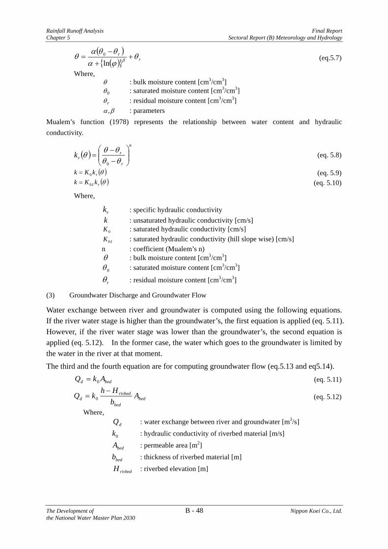
Rainfall Runoff Analysis Final Report Chapter 5 Sectoral Report (B) Meteorology and Hydrology
The Development of B - 48 Nippon Koei Co., Ltd. the National Water Master Plan 2030
(eq.5.7)
Where, : bulk moisture content [cm3/cm3]
: saturated moisture content [cm3/cm3] : residual moisture content [cm3/cm3] : parameters Mualem’s function (1978) represents the relationship between water content and hydraulic conductivity.
(eq. 5.8)
(eq. 5.9) (eq. 5.10)
Where,
: specific hydraulic conductivity : unsaturated hydraulic conductivity [cm/s] : saturated hydraulic conductivity [cm/s] : saturated hydraulic conductivity (hill slope wise) [cm/s] n : coefficient (Mualem’s n) : bulk moisture content [cm3/cm3] : saturated moisture content [cm3/cm3]
: residual moisture content [cm3/cm3]
(3) Groundwater Discharge and Groundwater Flow
Water exchange between river and groundwater is computed using the following equations. If the river water stage is higher than the groundwater’s, the first equation is applied (eq. 5.11). However, if the river water stage was lower than the groundwater’s, the second equation is applied (eq. 5.12). In the former case, the water which goes to the groundwater is limited by the water in the river at that moment. The third and the fourth equation are for computing groundwater flow (eq.5.13 and eq5.14).
(eq. 5.11)
(eq. 5.12)
Where, : water exchange between river and groundwater [m3/s] : hydraulic conductivity of riverbed material [m/s] : permeable area [m2] : thickness of riverbed material [m] : riverbed elevation [m]
r
r
ln0
0
r,
n
r
rrk
0
rkKk 0 rI kKk 0
rkk
0K
IK 0
0
r
bedd AkQ 0
bedbed
rivbedd A
b
HhkQ
0
dQ
0k
bedA
bedb
rivbedH

Final Report Rainfall Runoff Analysis Sectoral Report (B) Meteorology and Hydrology Chapter 5
Nippon Koei Co., Ltd. B - 49 The Development of the National Water Master Plan 2030
(eq. 5.13)
Where,
: groundwater flow : hydraulic conductivity
: groundwater slope (hydraulic gradient) : contact line length of two neighboring blocks : averaged aquifer thickness of the block
(eq. 5.14)
Where, : inflow (groundwater) from upper blocks and percolation [m3/s] : outflow from this block (groundwater) and other water losses [m3/s]
: area of the block [m2] : storage coefficient : groundwater table elevation [m]
(4) River Flow
In the river section, kinematic wave approximation is applied and the governing equations are as shown below. An explicit finite difference scheme has been used in the computer program.
(eq.5.15)
(eq.5.16)
Where, : river flow rate [m3/s]
: Manning’s roughness coefficient [s/m1/3]
: depth [m]
: slope
: cross-sectional area [m2] x,t : independent variables, spatial [m] and time [s] : lateral inflow [m2/s]
5.2.4 Conditions and Parameters
(1) Delineation of SHER Blocks
The subcatchment boundary, which was prepared in the NWMP (1992), was reviewed using detailed river lines data traced from a 1:50,000 topographic map and digital elevation model (DEM) of 90 m resolution grid from Shuttle Rader Topography Mission (SRTM), NASA. Some river lines cross over the subcatchment boundaries. MWI has requested the JICA Study Team to correct the subcatchment boundaries. The reviewed subcatchment boundaries are shown in Figure 5.2.1.
Tx
hKQg
0
gQ
0K
x
h
T
outin QQdt
dhSA
inQ
outQ
A
S
h
rxrr
ASRn
Q 21321
rrr q
t
A
x
Q
rQ
rn
rh
xS
rA
rq

Rainfall Runoff Analysis Final Report Chapter 5 Sectoral Report (B) Meteorology and Hydrology
The Development of B - 50 Nippon Koei Co., Ltd. the National Water Master Plan 2030
Source: JICA Study Team
Review of Subcatchment Boundaries using Detailed DEM
The discharging area and recharging area are divided for SHER blocks. The recharging area is where water from precipitation is transmitted downward to an aquifer. The discharging area is the opposite of the recharge area. These are located at areas where groundwater moves from the aquifer to the surface. Groundwater discharge occurs where the water table intersects the land surface. River channels appear when the groundwater table is higher than the bottom of the channel. High areas, such as hills or plateaus, are typically where aquifers are recharged. Low areas such as river valleys are where they discharge. However in many cases, the aquifer level is lower than river bed and the river water recharges the aquifer. Such areas also are treated as a discharging area in the SHER model, because the groundwater table is raised during the rainy season and the area becomes a discharging area.

Final Report Rainfall Runoff Analysis Sectoral Report (B) Meteorology and Hydrology Chapter 5
Nippon Koei Co., Ltd. B - 51 The Development of the National Water Master Plan 2030
In Kenya, there are many seasonal rivers. There are also many inland rivers in the Rift Valley, which has no river outlet where the river water submerge underground and disappear. It is necessary to define a discharging area for the seasonal rivers and inland rivers on the SHER model. The aerial imagery of Google Earth was referred for the delineation work of discharging and recharging area. Even if the water surface of the seasonal rivers and inland rivers are not visible on the aerial imagery, the unseen channel course can be supposed by the different colour of surface soil or the exuberance of vegetation in linear.
The total number of SHER blocks was 2,977 for the whole country. The calculation was conducted with time step of one day. The area outside of the country where rainfall runs into the inside of the country was modelled. The block numbers of each catchment are shown in the following figure and all block are shown in Figures 5.2.2 to 5.2.33. The sizes of each catchment areas are provided in the table below.
Catchment Area for Calculation
Catchment Area
Inside the country
Including outside of the county
Ratio
1 2 =1/2 LVN 19,012 19,928 95%LVS 27,425 29,676 92%RV 136,848 148,359 92%Athi 67,469 70,589 96%Tana 127,463 127,739 100%ENN 210,573 243,245 87%Total 588,790 639,537 92%
Note: The catchment area data were as per GIS data provided by WRMA. The above catchment area data were different from the one which were derived from the WRMA Catchment Management Strategies as shown in sub-section 1.3.1. Source: JICA Study Team
Source: JICA Study Team
Number of SHER Block Prepared for Whole Country
(2) Land Use
Land use condition is one of the key information to set the soil parameter of surface cover. Land use for the period of 2010 which was produced by remote sensing analysis was utilized for the rainfall-runoff analysis. The details of land use analysis are explained in the subsequent section (refer to Section 8 Land Use Analysis). In addition, the classification of paddy areas was
No. Catchment Area Blocks1 Lake Victoria North 3542 Lake Victoria South 2263 Rift Valley 7954 Athi 5655 Tana 5026 Ewaso Ng'iro North 535
Total 2,977
Recharging Area
Discharging Area

Rainfall Runoff Analysis Final Report Chapter 5 Sectoral Report (B) Meteorology and Hydrology
The Development of B - 52 Nippon Koei Co., Ltd. the National Water Master Plan 2030
supplemented by land cover information from FAO Africover. The land use classification is shown in the table below.
Land Use Classification
No. Classes Definition 1 Urban Residential, industrial and commercial complexes, transportation, communication and utilities. 2 Forest Deciduous, evergreen and mixed forest (natural and manmade forests). 3 Water All areas of open water, including streams, lakes and reservoirs. 4 Bare land Area of thin soil, sand, or rock, almost has no vegetation.
5 Mangrove Trees and shrubs growing below the high-water level of spring tides. Their root systems are
regularly inundated with saline water. They extend throughout tropical and sub-tropical ecosystems
6 Shrub/Woodland
A woody perennial plant, smaller than a tree, with several major branches arising from near the base of the main stem. It is mostly covered with woods or dense growths of trees and shrubs
7 Grassland An area in which the natural vegetation consists largely of perennial grasses, characteristic of subhumid and semi-arid climates. It is used for grazing or pasture.
8 Agricultural Crop fields, vegetable lands and cultivated areas (irrigated and non-irrigated vegetation).
9 Savannah A flat, grass covered area of tropical or subtropical regions, nearly treeless in some places but generally having a mix of widely spaced trees and bushes.
10 Wetland Areas of marsh, fen, peat land or water. They could be natural or artificial and the water
permanent or temporary, static or flowing, fresh, brackish or saline. Wetlands include areas of marine water whose depth during low tide must not exceed 6 m.
11 Paddy Paddy field
Source JICA Study Team
The land use classes listed above were reclassified for the hydrological model from the standpoint of surface soil status. For example, soil on forests and agricultural areas can be regarded as the same status of soil in view of hydraulic conductivity because the surface soil on these areas has large porosity. Paddy fields, mangrove areas and wetland areas can be put in the same soil status for hydrological model parameters because the surface soil on such areas are composed of silt or clay and their hydraulic conductivity is very small. The reclassification of the land use category for the SHER model is shown below.
Source JICA Study Team
Reclassification of Land Use Category for Hydrological Model
The ratio of impervious area to the land use category of “Urban” was evaluated by measuring pavement areas and roof areas in urban areas using aerial imagery of Google Earth. The hydrological process on impervious areas is quite different from pervious areas. Although the ratio of urban areas is very small in Kenya, it is important to set the ratio in the SHER model because the runoff ratio is
No. Land Use Category No.Re-classified Categoryfor Hydrological Model
1 Urban 1Compacted Loam &Impervious Area
2 Forest 2 Forest
3 Water 3 Savannah
4 Bare land 4 Bare Land5 Mangrove 5 Paddy6 Shrub/Woodland 6 Wetland7 Grassland 7 Water8 Agricultural9 Savannah10 Wetland11 Paddy
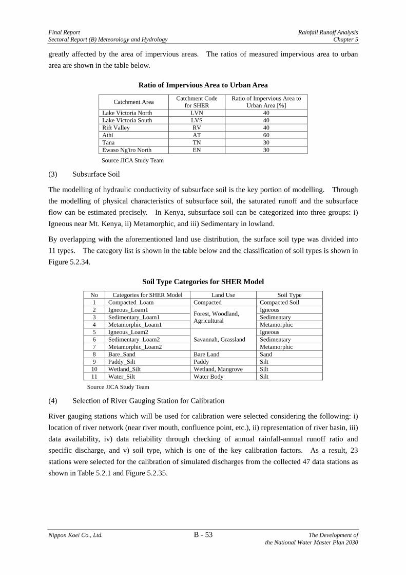
Final Report Rainfall Runoff Analysis Sectoral Report (B) Meteorology and Hydrology Chapter 5
Nippon Koei Co., Ltd. B - 53 The Development of the National Water Master Plan 2030
greatly affected by the area of impervious areas. The ratios of measured impervious area to urban area are shown in the table below.
Ratio of Impervious Area to Urban Area
Catchment Area Catchment Code for SHER
Ratio of Impervious Area to Urban Area [%]
Lake Victoria North LVN 40 Lake Victoria South LVS 40 Rift Valley RV 40 Athi AT 60 Tana TN 30 Ewaso Ng'iro North EN 30
Source JICA Study Team
(3) Subsurface Soil
The modelling of hydraulic conductivity of subsurface soil is the key portion of modelling. Through the modelling of physical characteristics of subsurface soil, the saturated runoff and the subsurface flow can be estimated precisely. In Kenya, subsurface soil can be categorized into three groups: i) Igneous near Mt. Kenya, ii) Metamorphic, and iii) Sedimentary in lowland.
By overlapping with the aforementioned land use distribution, the surface soil type was divided into 11 types. The category list is shown in the table below and the classification of soil types is shown in Figure 5.2.34.
Soil Type Categories for SHER Model
No Categories for SHER Model Land Use Soil Type 1 Compacted_Loam Compacted Compacted Soil 2 Igneous_Loam1 Forest, Woodland,
Agricultural
Igneous 3 Sedimentary_Loam1 Sedimentary 4 Metamorphic_Loam1 Metamorphic 5 Igneous_Loam2
Savannah, Grassland Igneous
6 Sedimentary_Loam2 Sedimentary 7 Metamorphic_Loam2 Metamorphic 8 Bare_Sand Bare Land Sand 9 Paddy_Silt Paddy Silt 10 Wetland_Silt Wetland, Mangrove Silt 11 Water_Silt Water Body Silt
Source JICA Study Team
(4) Selection of River Gauging Station for Calibration
River gauging stations which will be used for calibration were selected considering the following: i) location of river network (near river mouth, confluence point, etc.), ii) representation of river basin, iii) data availability, iv) data reliability through checking of annual rainfall-annual runoff ratio and specific discharge, and v) soil type, which is one of the key calibration factors. As a result, 23 stations were selected for the calibration of simulated discharges from the collected 47 data stations as shown in Table 5.2.1 and Figure 5.2.35.

Rainfall Runoff Analysis Final Report Chapter 5 Sectoral Report (B) Meteorology and Hydrology
The Development of B - 54 Nippon Koei Co., Ltd. the National Water Master Plan 2030
5.3 Calibration
5.3.1 Calibration with Observed River Flow Record
Simulation of the rainfall-runoff model was carried out with the prepared grid rainfall and the potential evapotranspiration which was evaluated by Hamon method for the present climate conditions in order to estimate the naturalized flow for assessment of renewable water resources. The model parameter was calibrated by comparing the observed discharge record at the selected river gauging stations and the simulation result. According to WRMA, the data quality of the river flow gauging after 1990’s has been deteriorated and the data before 1990 were recommended for calibration. Therefore, the period for calibration was from 1981 to 1990 for each gauging stations.
The saturated hydraulic conductivity of surface soil and the saturated hydraulic conductivity of aquifers were subjected to calibration in the SHER model. The results of calibrations are summarised in Figure 5.3.1. The comparison of the simulated discharge and observed discharge is shown in Figure 5.3.2. The calibrated parameter lists are shown in Tables 5.3.1 to 5.3.6. The applied efficiency criterion was to match the total annual discharges between the simulated and observed ones, and also to match the low flow discharges during the dry season between the simulated and observed ones.
As there was no flood data for calibration of the model, the simulated and observed values at high flows do not match very well. It is advised for WRMA to procure flood flow measuremet equipment to measure the flood discharge to accumulate data. (Ref. Main Report Part H, 3.2 Proposed Action Plans (2) a) iv))
The parameters for the subsurface soil were calibrated to be consistent and to be within the typical range. The results of the simulated river discharge were agreed with the observed record over the whole selected stations. It is possible to apply the developed rainfall-runoff model for evaluation of the water resources for un-gauging rivers, since the calibrated parameters have physical based meanings. Similarly, the model also can be applied for evaluation of future hydrological conditions and water resources with the bias corrected GCM data.
Source: JICA Study Team Selected Groundwater Level Gauging Wells for Verification of Calibrated SHER Model

Final Report Rainfall Runoff Analysis Sectoral Report (B) Meteorology and Hydrology Chapter 5
Nippon Koei Co., Ltd. B - 55 The Development of the National Water Master Plan 2030
5.3.2 Verification of Calibrated Model
(1) Groundwater Level
The observed groundwater level records for several wells were collected. Those wells are in use and the observed groundwater levels are affected by water pumping. The observed groundwater level data to which the influence of water pumping seems to be relatively lower than others were selected. The selected number of wells was 7. The comparisons of the simulated groundwater levels by calibrated SHER model and observed groundwater levels are shown in the following charts. They are agreed fairly.
Source: JICA Study Team Comparison of Groundwater Levels between Observed Record and Calculated by Calibrated SHER Model
0
100
200
300
400
500
600
700
800
900
1000
0
2
4
6
8
10
12
14
16
18
20
Monthly Rainfall [m
m]
GWL [GL.‐m
]
Groundwater Level (LVS. Trinity)
Monthly Rainfall [mm/month]
Calculated GWL [GL.‐m]
Observed GWL [GL.‐m]
0
100
200
300
400
500
600
700
800
900
1000
30
32
34
36
38
40
42
44
Monthly Rainfall [m
m]
GWL [GL.‐m
]
Groundwater Level (RV. Naivasha MW&I)
Monthly Rainfall [mm/month]
Calculated GWL [GL.‐m]
Observed GWL [GL.‐m]
0
100
200
300
400
500
600
700
800
900
1000
‐5
‐4
‐3
‐2
‐1
0
1
2
3
4
5
Monthly Rainfall [m
m]
GWL [GL.‐m
]
Groundwater Level (RV. Kakuma3)
Monthly Rainfall [mm/month]
Calculated GWL [GL.‐m]
Observed GWL [GL.‐m]
0
100
200
300
400
500
600
700
800
900
1000
30
31
32
33
34
35
36
37
38
39
40
Monthly Rainfall [m
m]
GWL [GL.‐m
]
Groundwater Level (AT. Eunice Wanjiru Gents Juja B/h C 11396)
Monthly Rainfall [mm/month]
Calculated GWL [GL.‐m]
Observed GWL [GL.‐m]
0
100
200
300
400
500
600
700
800
900
1000
10
11
12
13
14
15
16
17
18
19
20
Monthly Rainfall [m
m]
GWL [GL.‐m
]
Groundwater Level (AT. Ronald Ngala)
Monthly Rainfall [mm/month]
Calculated GWL [GL.‐m]
Observed GWL [GL.‐m]
0
100
200
300
400
500
600
700
800
900
1000
‐5
‐4
‐3
‐2
‐1
0
1
2
3
4
5
Monthly Rainfall [m
m]
GWL [GL.‐m
]
Groundwater Level (TN. Tyaa Kamuthale)
Monthly Rainfall [mm/month]
Calculated GWL [GL.‐m]
Observed GWL [GL.‐m]
0
100
200
300
400
500
600
700
800
900
1000
10
12
14
16
18
20
22
24
Monthly Rainfall [m
m]
GWL [GL.‐m
]
Groundwater Level (EN. Backlit)
Monthly Rainfall [mm/month]
Calculated GWL [GL.‐m]
Observed GWL [GL.‐m]

Rainfall Runoff Analysis Final Report Chapter 5 Sectoral Report (B) Meteorology and Hydrology
The Development of B - 56 Nippon Koei Co., Ltd. the National Water Master Plan 2030
(2) Water content of Surface Soil
The Advanced Microwave Scanning Radiometer (AMSR) mounted on satellites which was launched by Japan Aerospace Exploration Agency (JAXA) is a passive sensor that measures weak microwaves radiated from the Earth at several frequencies. Estimated soil moisture data are derived from the observed microwave. The algorithm for transformation to soil moisture was developed by Prof. Toshio Koike of University of Tokyo.
The estimated soil moisture data was obtained from the AMSR web site (http://sharaku.eorc.jaxa.jp/AMSR/index.html) from 2003 to 2010 and the calculated soil moisture by calibrated SHER model were compared with those AMSR data. The calculated soil moisture of sub-surface blocks of SHER model were area averaged for each cachment, LVNCA, LVSCA RVCA, ACA, TCA and ENNCA. On the whole catchments, the calculated soil moistures reproduced the estimated that by AMSR very well. From those comparison, the calibrated SHER model represents the hydrological processes adequately.

Final Report Rainfall Runoff Analysis Sectoral Report (B) Meteorology and Hydrology Chapter 5
Nippon Koei Co., Ltd. B - 57 The Development of the National Water Master Plan 2030
Source: JICA Study Team
Comparison of Area Averaged Soil Moisture Data between Calculated and eEtimated by AMSR-E
0
100
200
300
400
500
600
700
800
900
10000
0.05
0.1
0.15
0.2
0.25
0.3
0.35
2003/01 2004/01 2005/01 2006/01 2007/01 2008/01 2009/01 2010/01
Rainfall [mm/m
onth]
Soil Moisture [cm3/cm3]
LVN
Rainfall AMSR_insolation
AMSR_shaded SHER
0
100
200
300
400
500
600
700
800
900
10000
0.05
0.1
0.15
0.2
0.25
0.3
0.35
2003/01 2004/01 2005/01 2006/01 2007/01 2008/01 2009/01 2010/01
Rainfall[m
m/m
onth]
Soil M
oisture [cm3/cm
3]
LVS
Rainfall AMSR_insolation
AMSR_shaded SHER
0
100
200
300
400
500
600
700
800
900
10000
0.05
0.1
0.15
0.2
0.25
0.3
0.35
2003/01 2004/01 2005/01 2006/01 2007/01 2008/01 2009/01 2010/01
Rainfall [m
m/m
onth]
Soil M
oisture [cm3/cm
3]
RV
Rainfall AMSR_insolation
AMSR_shaded SHER
0
100
200
300
400
500
600
700
800
900
10000
0.05
0.1
0.15
0.2
0.25
0.3
0.35
2003/01 2004/01 2005/01 2006/01 2007/01 2008/01 2009/01 2010/01
Rainfall [m
m/m
onth]
Soil M
oisture [cm3/cm
3]
AT
Rainfall AMSR_insolation
AMSR_shaded SHER
0
100
200
300
400
500
600
700
800
900
10000
0.05
0.1
0.15
0.2
0.25
0.3
0.35
2003/01 2004/01 2005/01 2006/01 2007/01 2008/01 2009/01 2010/01
Rainfall [mm/m
onth]
Soil Moisture [cm3/cm3]
TN
Rainfall AMSR_insolation
AMSR_shaded SHER
0
100
200
300
400
500
600
700
800
900
10000
0.05
0.1
0.15
0.2
0.25
0.3
0.35
2003/01 2004/01 2005/01 2006/01 2007/01 2008/01 2009/01 2010/01
Rainfall [m
m/m
onth]
Soil Moisture [cm3/cm3]
EN
Rainfall AMSR_insolation
AMSR_shaded SHER

Rainfall Runoff Analysis Final Report Chapter 5 Sectoral Report (B) Meteorology and Hydrology
The Development of B - 58 Nippon Koei Co., Ltd. the National Water Master Plan 2030
5.4 Result of Rainfall-Runoff Analysis
5.4.1 Simulation of Present and Future Runoff
The naturalized runoff for the present climate condition was estimated with the present climatology inputs from 1991 to 2010. For the future climate conditions, a rainfall-runoff analysis was carried out for a 20-year time sequence using future climate of 11 GCMs with bias correction. Future runoff was estimated for the 2030 and 2055 climates. The annual catchment area precipitation (rainfall) used for the rainfall-runoff analysis are shown below.
Annual Catchment Area Average Precipitation (Unit: mm/year)
Catchment Area Area (km2) Present (2010) Climate
2030 Climate
2055 Climate
Lake Victoria North 19,012 1,415 1,505 1,601 Lake Victoria South 27,425 1,277 1,372 1,451 Rift Valley 136,848 509 583 653 Athi 67,469 808 881 916 Tana 127,463 837 899 935 Ewaso Ng'iro North 210,573 510 577 623 Whole Country 588,790 679 750 801
Source: JICA Study Team
The average monthly rainfall by sub-basin is presented in Table 5.4.1 and 5.4.2.
The surface water runoff by catchment area for the years 2010, 2030 and 2055 are shown below.
Annual Surface Water Runoff by Catchment Area (Unit: MCM/year)
Catchment Area Area (km2) Present (2010) Climate
2030 Climate
2055 Climate
Lake Victoria North 19,012 4,626 4,969 5,455 Lake Victoria South 27,425 4,773 5,749 7,005 Rift Valley 136,848 2,457 3,045 3,794 Athi 67,469 1,198 1,334 1,711 Tana 127,463 5,858 7,261 7,383 Ewaso Ng'iro North 210,573 1,725 2,536 1,361
Total 588,790 20,637 24,894 26,709
Source: JICA Study Team
As shown in the table above, the annual surface water runoff in all catchment areas except the Ewaso Ngiro North Catchment Area (ENNCA) are predicted to increase toward 2055. ENNCA has a trend to increase toward 2030, but would then decrease toward 2055. ENNCA has a climatic characteristic that pressure of dryness is the highest among six catchment areas and 90% of precipitation evaporates even at present. The impact of future climate change is increase of both precipitation and temperatures, but the difference between precipitation and temperature is small compared with other catchment areas. In 2030, the precipitation exceeds the actual evapotranspiration and in 2055 vice versa. For this the annual surface water runoff in 2055 decreases against that in 2030. The average monthly surface water runoff by sub-basin are presented in Tables 5.4.3 and 5.4.4. The monthly precipitation and surface water runoff for each year from 1991 to 2010 and from 2021 to 2040 are presented in Databook Part A.

Final Report Rainfall Runoff Analysis Sectoral Report (B) Meteorology and Hydrology Chapter 5
Nippon Koei Co., Ltd. B - 59 The Development of the National Water Master Plan 2030
5.4.2 Flow Duration Curve
The flow duration curve was prepared for a 20-year time sequence runoff. The procedure for the preparation of flow duration curve is explained as follows:
i) The simulated runoff results were grouped annually. Then, the flow duration curve for each year was prepared. A total of 20 flow duration curves was produced for one station.
ii) By averaging these curves, one represented flow duration curve was prepared.
For the future climate conditions, the flow duration curve was produced for each GCM output. The ensemble average curve was prepared by averaging the 11 flow duration curves.
Schematic Image of Ensemble Average of Flow Duration Curves
5.4.3 Comparison of Flow Duration Curve
The flow duration curves for the present and future climate conditions were compared as shown in Figure 5.4.1. According to the flow duration curves of the calculated runoff for the present and future climate conditions, high water flow such as runoff in the rainy season increases due to the increase of future rainfall, while low water flow such as runoff in the dry season will not change.
5.5 Impact of Climate Change on Hydrological Conditions
5.5.1 Evaluation of Hydrological Water Budget
All of hydrological process flux can be obtained from the calculation output of SHER model. The hydrological water balance of six catchment areas for present (2010) and future (2030 and 2055) conditions were evaluated. The potential evapotranspiration (PET) estimated by Hamon method was utilized for the hydrological water budget basically as explained in Section 4.9. The groundwater recharge of whole country was estimated at 56 BCM/yr (95mm/year) for present condition. In order to study the amount of the water resources of Kenya more comprehensively, the hydrological water budget was studied by applying the PET estimated by FAO Penman-Monteith (FAO-PM) method. The procedure is as mentioned below:
a) The difference of the both of PETs were calculated; HamPM ETETET , where ETPM is potential evapotranspiration evaluated by FAO-PM method and ETHam is that of Hamon method.
28
Mean Annual Curves of 11 GCMs input

Rainfall Runoff Analysis Final Report Chapter 5 Sectoral Report (B) Meteorology and Hydrology
The Development of B - 60 Nippon Koei Co., Ltd. the National Water Master Plan 2030
b) The groundwater recharge which is the percolation flux from sub-surface soil layer to aquifer, was corrected by subtraction ET from the percolation calculated under the condition of Hamon PET; Rech_corrected = Rech - ET
c) The correction processed repeated for every SHER model blocks day by day.
Then, the corrected groundwater recharge under the condition of FAO-PM PET was estimated at 21.5 BCM/yr (36mm/year) for whole country.
There are a certain range of uncertainty on the evaluation of groundwater recharge and soil evapotranspiration. It is very difficult to predict the amount of the groundwater recharge with unfailing accuracy. The groundwater analysis is discussed in Chapter 7 in detail.
The estimated hydrological water budget for the PET by Hamon method illustrated in Figure 5.5.1 and that for the PET by FAO-PM method is shown in Figure 5.5.2. Figure 5.5.3 shows the change of annual surface runoff volume for 2010, 2030 and 2055.
The distribution of groundwater evapotranspiration is discussed in Chapter 7.
5.5.2 Soil Evapotranspiration
The soil evapotranspiration was obtained from the rainfall-runoff model analysis for the present and the future climate conditions of 11 GCMs. The ensemble analysis results of the actual soil evapotranspirations for the potential evapotranspiration estimated by Hamon method are shown in Figure 5.5.4 for annual amount and in Figures 5.5.5 to 5.5.8 for seasonal amount. Those for FAO-PM method are shown in Figures 5.5.9 to 5.5.13. They are tabulated below by catchment area.
Annual Soil Evapotranspiration Estimated under Hamon PET Condition (Unit: mm/year)
Catchment Area Area (km2) Present (2010) Climate
2030 Climate
2055 Climate
Lake Victoria North 19,012 800 854 898 Lake Victoria South 27,425 784 835 864 Rift Valley 136,847 440 506 565 Athi 67,469 687 756 777 Tana 127,462 671 733 774 Ewaso Ng'iro North 210,573 449 514 566 Whole Country 588,790 549 613 659
Note: The area was measured by the GIS data provided by WRMA. Source: JICA Study Team.
Annual Soil Evapotranspiration Estimated under FAO-PM PET Condition (Unit: mm/year)
Catchment Area Area (km2) Present (2010) Climate
2030 Climate
2055 Climate
Lake Victoria North 19,012 1,102 1,178 1,230 Lake Victoria South 27,425 1,019 1,085 1,118 Rift Valley 136,847 482 553 617 Athi 67,469 741 813 837 Tana 127,462 731 791 832 Ewaso Ng'iro North 210,573 475 541 593 Whole Country 588,790 608 675 723
Note: The area was measured by the GIS data provided by WRMA. Source: JICA Study Team.

Final Report Rainfall Runoff Analysis Sectoral Report (B) Meteorology and Hydrology Chapter 5
Nippon Koei Co., Ltd. B - 61 The Development of the National Water Master Plan 2030
The annual evapotranspiration will increase over the whole country. The difference in evapotranspiration in the projected 2030 climate from present conditions was evaluated as 70 mm/year under both of PET evaluation methods, and the difference in the 2055 climate will be increased to 100 to 110 mm/year.
The difference of future evapotranspiration from the present climate of the long rainy season (MAM) will increase all over the country in the future. Meanwhile, the amount of evapotranspiration of the long dry season (JJA) will not change drastically and those of Tana and Athi catchments will decrease in the future.
5.5.3 Precipitation Minus Soil Evapotranspiration
The spatial distribution of the future annual precipitation minus the actual soil evapotranspiration (P-SET) will be almost unchanged from the present distribution. However, the northern part of the Rift Valley Catchment and the northern part of the Ewaso Ng'iro North Catchment are expected to be drier as shown in Figure 5.5.14 for the potential evapotranspiration estimated by Hamon method. The seasonal ensemble analysis are shown in Figures 5.5.15 to 5.5.18. Those for the potential evapotranspiration estimated by Hamon method are shown in Figures 5.5.19 to 5.5.23.
From the seasonal view, even though the increase of water resources is expected in the rainy seasons, most of the country will be drier in the dry season (June–August). Renewable water resources are more unevenly distributed in terms of spatial and temporal viewpoints in the future. The acceleration of unevenness of the temporal and spatial distribution is the impact of climate change on hydrological conditions of Kenya.
5.5.4 Groundwater Recharge
Groundwater is an important water resource for ASALs of Kenya. The groundwater recharge was estimated through rainfall-runoff analysis. The estimated annual groundwater recharges by catchment areas for the years present, 2030, and 2055 are shown below. Groundwater recharge was estimated based on the rainfall – runoff analysis. Considering future climate change, annual rainfall was estimated to be increased and the annual evapotranspiration was estimated to be increased. These are the impact of the climate change which is derived from analysis using GCM results. These two impacts have opposite vector to the water resources.
Annual Groundwater Recharge by Catchment Area under Hamon PET Condition (Unit: MCM/year)
Catchment Area Area (km2) Present (2010) Climate
2030 Climate
2055 Climate
Lake Victoria North 19,012 7,083 7,412 7,917 Lake Victoria South 27,425 8,743 8,983 9,096 Rift Valley 136,847 6,863 7,467 8,250 Athi 67,469 7,002 7,099 7,686 Tana 127,462 15,298 13,977 13,217 Ewaso Ng'iro North 210,573 10,986 10,642 10,708 Total 588,790 55,975 55,580 56,874
Note: The area was measured by the GIS data provided by WRMA. Source: JICA Study Team.

Rainfall Runoff Analysis Final Report Chapter 5 Sectoral Report (B) Meteorology and Hydrology
The Development of B - 62 Nippon Koei Co., Ltd. the National Water Master Plan 2030
Annual Groundwater Recharge by Catchment Area under FAO-PM PET Condition (Unit: MCM/year)
Catchment Area Area (km2) Present (2010) Climate
2030 Climate
2055 Climate
Lake Victoria North 19,012 1,326 1,251 1,612 Lake Victoria South 27,425 2,294 2,112 2,126 Rift Valley 136,847 1,126 1,126 1,209 Athi 67,469 3,345 3,303 3,649 Tana 127,462 7,719 6,520 5,840 Ewaso Ng'iro North 210,573 5,660 5,095 4,851 Total 588,790 21,470 19,407 19,287
Note: The area was measured by the GIS data provided by WRMA. Source: JICA Study Team. The amount of the groundwater recharge estimated under the FAO-PM PET condition is about half of the amount under the Hamon PET condition.
Evapotranpiration estimated with Hamon
Evapotranpiration estimated with FAO Penman
By changing Hamon to FAO Penman, the evapotranspiration increases by 34.5 BCM and becomes 358.0 BCM/yr. (608 mm/year.), meaning about 10% increase from the original 323.5 to 358.0 BCM/year. Because the evapotranspiration increases and a surface runoff value remain unchanged, the groundwater recharge decreases by 34.5 BCM/year (the same amount of evapotranspiration increase) and becomes 21.5 BCM/year (36mm/year.). In this manner, the small increase in evapotranspiration gives large decrease in groundwater recharge which is about 60% of the groundwater recharge estimated by Hamon method (56.0 BCM/year).
The spatial distributions of ensemble mean annual groundwater recharges under Hamon PET condition are shown in Figure 5.5.24 for whole country and in Figures 5.5.25 to 5.5.28 for seasonal change. Those under FAO-PM PET condition are shown in Figures 5.5.29 to 5.5.33.
The amount and distribution of groundwater recharge are expected not to be changed drastically in view of the annual amount and distribution. The recharge volume will be increased at wet areas, particularly in the middle and western area, while the recharge volume at ASALs will decrease.
The change of the recharge amount in the long dry season, from June to August, is shown in Figure 5.5.14, and the groundwater recharge of the dry season will decrease in most parts of the country.
The further unevenness of spatial and temporal can also be expected from the aspect of the groundwater recharge.
The change of groundwater recharge amounts between 2010 and 2055 is small under Hamon PET condition as the difference is only 2% of the groundwater recharge amount, while the difference under
Precipitation (P)400.1 BCM/yr
(679 mm/yr)
Evapotranspiration (Ev)323.5 BCM/yr
(549 mm/yr)
Renewable WR(P – Ev)
76.6 BCM/yrPercolation63.5 BCM/yr
GW Discharge7.5 BCM/yr
Surface Runoff20.6 BCM/yr
(Renewable SW)
Direct Runoff13.1 BCM/yr
GW Recharge56.0 BCM/yr
(95 mm/yr)(Renewable GW)
Precipitation (P)400.1
Evapotranspiration (Ev)323.5 358.0
(+34.5)Renewable WR
(P – Ev)76.6 42.1
(-34.5) Percolation63.5 29.0
(-34.5)
GW Discharge7.5
Surface Runoff20.6
(Renewable SW)
Direct Runoff13.1
(Unit: BCM/yr)
GW Recharge56.0 21.5
(-34.5)(Renewable GW)

Final Report Rainfall Runoff Analysis Sectoral Report (B) Meteorology and Hydrology Chapter 5
Nippon Koei Co., Ltd. B - 63 The Development of the National Water Master Plan 2030
FAO-PM PET condition comes to 10%, but it is considered to be not significant difference considering accuracy of estimation of the evapotranspiration and uncertainty of the climate change analysis. The groundwater recharge amount will remain almost unchanged toward future.
5.6 Evaluation of Water Resources
5.6.1 Annual Renewable Water Resources
Renewable water resources are computed on the basis of the water cycle. The total of annual renewable surface water resources and annual groundwater recharge were estimated by multiplying the values of rainfall minus the soil evapotranspiration by catchment area. The total annual renewable surface water resources and annual groundwater recharge by catchment for the years of present , 2030 and 2055 were estimated, as shown below.
Annual Renewable Water Resources under Hamon PET Condition (Unit: MCM/year)
Catchment Area
Present (2010) Climate
2030 Climate
2055 Climate
Lake Victoria North 11,709 12,379 13,371 Lake Victoria South 13,516 14,732 16,101 Rift Valley 9,319 10,512 12,045 Athi 8,199 8,434 9,397 Tana 21,156 21,239 20,600 Ewaso Ng'iro North 12,710 13,177 12,069 Total 76,609 80,473 83,583
Note: The area was measured by the GIS data provided by WRMA. Source: JICA Study Team
Annual Renewable Water Resources under FAO-PM PET Condition (Unit: MCM/year)
Catchment Area
Present (2010) Climate
2030 Climate
2055 Climate
Lake Victoria North 5,952 6,220 7,067 Lake Victoria South 7,067 7,861 9,131 Rift Valley 3,583 4,171 5,003 Athi 4,543 4,637 5,360 Tana 13,577 13,781 13,223 Ewaso Ng'iro North 7,385 7,631 6,212 Total 42,107 44,301 45,996
Note: The area was measured by the GIS data provided by WRMA. Source: JICA Study Team
As shown in the above table, the renewable water resources in all catchments except Tana and Ewaso Ng'iro North have an increasing trend. The eastern part of the country, in which Tana and Ewaso Ng’iro North catchments are placed, will be stronger drying pressure rather than the other area. The renewable water resources in Ewaso Ng'iro North Catchment are expected to increase in 2030, but will decrease in 2055 due to the increase of potential evapotranspiration. A contradicted trend was seen due to the sensitive balance of precipitation increase and evaporation increase. From a planning point of view, the present values were decided to be applied considering the uncertainty of GCM projections.

Rainfall Runoff Analysis Final Report Chapter 5 Sectoral Report (B) Meteorology and Hydrology
The Development of B - 64 Nippon Koei Co., Ltd. the National Water Master Plan 2030
The amount of the renewable water resources under FAO-PM PET condition was estimated as half of that of the Hamon method. In order to avoid the excessive development, it is recommended to use the water resources estimated by the FAO-PM PET condition in this study.
5.6.2 Annual Renewable Surface Water Resources
The renewable surface water resources were estimated by summation of the annual river runoff at most downstream river reaches within the catchment through the rainfall-runoff analysis. The estimated annual renewable surface water resources by catchment for the years of 2010, 2030 and 2055 are shown in the table in Section 5.4.1 as annual surface water runoff. The specific annual renewable surface water resources by sub-basin for the year 2010 are shown in Figure 5.6.1. The difference of annual renewable surface water between 2010 and 2030 is shown in Figure 5.6.2.
5.6.3 Annual Renewable Groundwater Resources
The renewable groundwater resources were estimated as groundwater recharge within the catchment through the rainfall-runoff analysis. The estimated annual renewable groundwater resources by catchment for the years of 2010, 2030 and 2055 are shown in the tables in Section 5.5.4 as annual groundwater recharge. The annual groundwater recharge much varies by variation of the evapotranspiration. As seen in the tables, the amount of the renewable groundwater resources under FAO-PM PET condition comes to 21.5 BCM/year which is less than half of that of Hamon PET condition of 56 BCM/year. The distribution of groundwater recharge is discussed in Chapter 7.
5.7 Recommendation for Further Study
For the hydro-meteorological analysis, a lot of existing rainfall and river discharge data were checked and it was known that the existing data have many gaps in observation. The accuracy of analysis depends on reliability of the data used.
It is recommended to continuously carry out the observation of rainfall and river discharges at the key stations to improve the reliability of the data.

Final Report Flood Analysis Sectoral Report (B) Meteorology and Hydrology Chapter 6
Nippon Koei Co., Ltd. B - 65 The Development of the National Water Master Plan 2030
CHAPTER 6 FLOOD ANALYSIS
6.1 Approach to the Analysis
One of the important points of climate change impact on hydrological conditions is that flood flow is expected to increase. The probable flood discharge was evaluated in this chapter.
The data availability of observed flood data of Kenya is not sufficient in view of the number of stations and temporal availability. The stations which have sufficient data availability were selected for the evaluation of probable flood discharge. Several probability density function (PDFs) were examined to estimate probable flood discharge. The standard least-squares criterion (SLSC) is the index for evaluation of fitness of the calibrated PDF to the plotted sample dataset by plotting position method. The most appropriate PDF, which indicates the smallest value of SLSC, was selected.
The output of the rainfall-runoff analysis covered the whole of the country. Simulated discharge data sets were assessed, not only for present conditions but also future conditions, considering climate change impacts. Probable flood discharges at every river point, which were modelled for runoff analysis, were evaluated in the same way as that for observed data. There were 11 scenarios for the future because 11 GCMs were selected for the study of climate change impact. The assessed 11 probable flood discharges were averaged and the ensemble mean and confidential interval for every point were evaluated.
Finally, the assessed probable discharge for the present and the future, particularly in 2030 and 2055, were aligned with the catchment area on a log-log plot. The regression curves for the regional plots were calculated. The regional area-flood discharge curve can be applied for trial evaluation for river planning and dam planning. Although the detailed study for flood discharge would be necessary for the detailed planning.
6.2 Evaluation of Probable Flood Based on Observed Discharge
6.2.1 Data Availability and Extraction of Annual Maximum Discharge
The daily discharge data for 47 river gauging stations were corrected for this study. The data availability for each year was tabulated in Table 5.2.1. For flood analysis, annual maximum discharge is most important and most basic value. It might be difficult to know the maximum discharge for the year that data availability is too low. For evaluating probable quantity by statistical approach, 20 or more samples are necessary. The numbers of valid years for each station were counted. The valid year is defined as the annual data availability is over 80%. The stations with more than 15 valid years were selected for the subjected stations for frequency analysis and the valid year counting result are shown in Table 6.2.1. The hydrographs of selected stations are shown in Figures 6.2.1 to 6.2.18.
Annual maximum floods for the selected stations were extracted from the observed record and are given in Table 6.2.2.

Flood Analysis Final Report Chapter 6 Sectoral Report (B) Meteorology and Hydrology
The Development of B - 66 Nippon Koei Co., Ltd. the National Water Master Plan 2030
6.2.2 Probable Flood Based on Observed Discharge Record
(1) Probability Density Functions
The probable flood discharges were examined using five PDFs. The applied PDFs are Log Normal Distribution (LN3), Gumbel Distribution, Log Pearson III Distribution (LP3), Generalized Extreme Value Distribution (GEV) and Square-Root Exponential Type Distribution (SQRT-ET). The formulas are described below.
Log Normal Distribution (LN3):
Probability density function
axyax
axxf
y
y
y
ln,
ln21exp
21
2
(eq. 6.1)
Cumulative distribution function
dttz
axxF
y
y 2
21exp
21,
ln
(eq. 6.2)
Where, a is a parameter, y is mean, and y is standard deviation of y.
Gumbel Distribution:
Gumbel distribution function is also known as the double exponential function.
Probability density function
x
a
cx
a
cx
axf ,expexp1
(eq. 6.3)
Cumulative distribution function
a
cxxF expexp (eq. 6.4)
Where, a and c are parameters of the function.
Log Pearson III Distribution (LP3):
Probability density function
xcaa
cx
a
cx
xbaxf
b
)exp(,0,lnexpln1 1
(eq. 6.5)
Cumulative distribution function
0exp1,ln0
1
adtttb
Ga
cxGxF b
(eq. 6.6)
Where, a, b and c are parameters of the function.

Final Report Flood Analysis Sectoral Report (B) Meteorology and Hydrology Chapter 6
Nippon Koei Co., Ltd. B - 67 The Development of the National Water Master Plan 2030
Generalized Extreme Value Distribution (GEV):
Probability density function
01exp11111
ka
cxk
a
cxk
axf
kk
(eq. 6.7)
Cumulative distribution function
01exp1
k
a
cxkxF
k
(eq. 6.8)
Where, a, c and k are parameters of the function.
Square-Root Exponential Type Distribution (SQRT-ET):
Probability density function
0exp1exp2
xbxbxabxab
xf (eq. 6.9)
Cumulative distribution function
0exp1exp xbxbxaxF (eq. 6.10)
Where, a and b are parameters of the function.
(2) Probable Flood Discharge
Probable flood discharges were calculated using the five PDFs mentioned above. The five PDFs evaluated the fitness of the estimated PDF to the sampled annual maximum data. The SLSC was applied for the evaluation of the fitness, which is widely used to quantify the fitness of extreme distribution functions to data. The best fitted PDF, which has the lowest SLSC score among the five PDFs, was selected. An SLSC score of 0.04 was used as a criterion of the common fitness validity. The evaluated probable floods which have an SLSC score of more than 0.04 were considered invalid. The evaluated probable floods for the selected river gauging stations are shown in Table 6.2.3.
6.3 Assessment of Probable Flood in Future and Regional Area-Flood Curve
The rainfall-runoff analysis was carried out for the whole country, and the dates for present (1981-2000), as well as the years of 2030 (2021-2040) and 2055 (2046-2065) were evaluated. For the evaluation of future hydrological conditions, all data of the 11 selected GCMs were applied for the input of the runoff analysis. The probable flood discharges of all river reaches in Kenya were evaluated based on the simulated river discharge for all GCMs in the future condition, the same way as the evaluation based on observed data. The 11 probable discharges were averaged and the ensemble mean of probable discharge was calculated for every river reach. The probable flood discharges of ensemble mean were plotted with the catchment area at corresponding river reaches. Then, regression analysis was carried out, and the regression curves were evaluated for every basin. The basin code which was shown in the figure and tables of this chapter is tabulated in Table 6.3.1. This code was numbered for the runoff model. The maps of the basins are shown in Figures 5.2.2 to 5.2.33.

Flood Analysis Final Report Chapter 6 Sectoral Report (B) Meteorology and Hydrology
The Development of B - 68 Nippon Koei Co., Ltd. the National Water Master Plan 2030
The equations of regression curve of area-flood relation are given in Table 6.3.2. The probable flood discharges of Kenya are expected to increase for the whole region. It is difficult to discuss about the probable discharge in a high degree of accuracy because there are many kinds of problems in the process. Such problems include limited data availability of the observed river flow in terms of spatial and temporal, and low reliability of observed flood discharges. These evaluated results can be used as a rough estimation for the regional flood characteristics. It is highly recommended to further carry out a detailed study for the detailed planning or the design stage.
Final Report Groundwater Analysis Sectoral Report (B) Meteorology and Hydrology Chapter 7
Nippon Koei Co., Ltd. B - 69 The Development of the National Water Master Plan 2030
CHAPTER 7 GROUNDWATER ANALYSIS
7.1 Introduction
Groundwater has played and will continue to play a vital role in the development of various areas in Kenya. For example, the City of Nairobi relies extensively on groundwater to meet domestic, commercial and industrial needs that cannot be met by surface water supply. A number of major towns rely either exclusively or extensively on groundwater such as Malindi and Nakuru. Numerous rural communities across the country use groundwater from boreholes equipped with hand pumps. In the North Eastern Province where deep groundwater is the only perennial source of water for humans and livestock, economic activity is seriously hampered without groundwater. The agricultural export sector has grown rapidly with the help of groundwater development in many areas, notably in the Rift Valley, Athi and Ewaso Ng’iro Catchments. However, groundwater abstraction exceeding sustainable yield is seen, leading to water level decline (depletion) and water quality deterioration (Guidelines for Artificial Groundwater Recharge, WRMA, 2012).
The groundwater analysis in this study was carried out to understand the occurrence, distribution and movement of groundwater in the country. Major outputs of groundwater analysis include evaluation of sustainable yield of groundwater and preparation of the groundwater potential map showing the evaluation results.
The years subject to the groundwater analysis are same as those for the rainfall-runoff analysis in Section 5.1 as below.
a) Year 2010(Present): The year represents the present hydrometeorological conditions. The present (2010) climate in this study expresses the climate during 1991 – 2010.
b) Year 2030: Target year for formulation of NWMP 2030. The 2030 climate in this study expresses the climate during 2021 – 2040.
c) Year 2055: The year to evaluate the water resources around 2050 taking into account climate change. The 2055 climate in this study expresses the climate during 2046 – 2065. It can be expressed by Year 2050 in the formulation of NWMP2030.
As for the depth of groundwater, the deepest existing boreholes for water use purpose are at around 400 to 500 m at maximum. Therefore, this depth was regarded as the maximum for exploitation in the study. It was decided not to consider water use deeper than this, such as geothermal water.
7.1.1 Objective
Evaluation of groundwater potential is essential to develop groundwater resources strategically and efficiently. The objective of groundwater analysis is to know the source, distribution and movement of groundwater. The results of the analysis will be illustrated as a groundwater potential map. Groundwater potential was evaluated in the previous master plan; however, groundwater abstraction has been increasing in accordance with economic growth. An evaluation update for groundwater potential is needed, utilizing the latest available data.

Groundwater Analysis Final Report Chapter 7 Sectoral Report (B) Meteorology and Hydrology
The Development of B - 70 Nippon Koei Co., Ltd. the National Water Master Plan 2030
7.1.2 Approach to the Analysis
(1) Definition
There are several definitions of groundwater potential according to previous researches or studies. To avoid misunderstanding the term “groundwater potential”, the following definitions were introduced in this study:
1) Renewable Groundwater Resources
Groundwater balance is indicated in the following figure of the annual water budget (similar to Figure 5.6.2). In the figure, renewable groundwater resource is equivalent to annual volume of “percolation”, given by hydro-meteorological analysis in Chapter 5. Percolation is the movement of water through fractures or interstices of a rock or soil. The amount of renewable groundwater resources for the years present (2010), 2030 and 2055 are estimated as shown in the table below.
Note: Soil evapotranspiration is estimated by the FAO PM method Source: JICA Study Team
Groundwater Balance
Precipitation Soil Evapotranspiration[MCM/yr] [mm/yr] Ratio [MCM/yr] [mm/yr] Ratio
Present 400,066 679 100% Present 357,959 608 89%2030 441,594 750 100% 2030 397,293 675 90%2055 471,858 801 100% 2055 425,862 723 90%
P-E Direct/Intermediate Runoff[MCM/yr] [mm/yr] Ratio [MCM/yr] [mm/yr] Ratio
Present 42,107 71 11% Present 13,133 22 3%2030 44,301 75 10% 2030 15,098 26 3% River Flow2055 45,996 78 10% 2055 15,907 27 3% [MCM/yr] [mm/yr] Ratio
Present 20,637 35 5%2030 24,894 42 6%2055 26,709 45 6%
Percolation[MCM/yr] [mm/yr] Ratio
Present 28,974 49 7% Groundwater Evapotranspiration2030 29,203 49 7% Groundwater Discharge [MCM/yr] [mm/yr] Ratio2055 30,089 51 6% [MCM/yr] [mm/yr] Ratio Present 21,314 36 5.3%
Present 7,504 13 2% 2030 19,305 33 4.4%2030 9,796 16 2% 2055 19,231 33 4.1%
Recharge to Groundwater 2055 10,802 18 2%[MCM/yr] [mm/yr] Ratio
Present 21,470 36 5%2030 19,407 33 4%2055 19,287 33 4% Flow Out of the Boundary
[MCM/yr] [mm/yr] RatioPresent 156 0.000 0.04%2030 102 0.000 0.02%2055 56 0.000 0.01%
Water Budget of Whole Country
The ratio [%] is a rate ofamount to the precipitation.
Ground Surface
Groundwater
RiverGroundwater

Final Report Groundwater Analysis Sectoral Report (B) Meteorology and Hydrology Chapter 7
Nippon Koei Co., Ltd. B - 71 The Development of the National Water Master Plan 2030
Renewable Groundwater Resources (Percolation) for Present (2010), 2030 and 2055 (Unit: MCM/year)
Catchment Area Present (2010)Climate
2030 Climate
2055 Climate
Lake Victoria North 4,543 4,624 5,030 Lake Victoria South 4,763 4,772 4,944 Rift Valley 2,459 2,779 3,244 Athi 3,159 3,232 3,662 Tana 8,533 8,321 8,056 Ewaso Ng'iro North 5,517 5,475 5,153 Total 28,974 29,203 30,089
Source: JICA Study Team
2) Renewable Groundwater Recharge
Renewable groundwater recharge is equivalent to “annual volume of “Recharge to groundwater’’ in the above figure. Recharge to groundwater is net amount of water added to an aquifer and is estimated as the rest of deriving “groundwater discharge” from “percolation”. The amount of renewable groundwater recharge for the years present (2010), 2030 and 2055 are estimated through rainfall-runoff analysis by SHER model as shown in the table below.
Recharge to Groundwater for 2010, 2030 and 2050 (Unit: MCM/year)
Catchment Area Present (2010)Climate
2030 Climate
2055 Climate
Lake Victoria North 1,326 1,251 1,612 Lake Victoria South 2,294 2,112 2,126 Rift Valley 1,126 1,126 1,209 Athi 3,345 3,303 3,649 Tana 7,719 6,520 5,840 Ewaso Ng'iro North 5,660 5,095 4,851
Total 21,470 19,407 19,287 Source: JICA Study Team
3) Sustainable Yield
Sustainable yield is defined as the amount of groundwater which could be developed sustainably without an undesirable impact.
(2) Flow of Groundwater Analysis
The flow of the analysis to estimate the sustainable yield of groundwater is shown in the following chart. To verify how renewable groundwater recharge flows in the aquifer as groundwater and analyses the mechanism of groundwater flow, a groundwater flow simulation for the whole of Kenya is made using MODFLOW, originally developed by U.S. Geological Survey, and then the sustainable yield is estimated.

Groundwater Analysis Final Report Chapter 7 Sectoral Report (B) Meteorology and Hydrology
The Development of B - 72 Nippon Koei Co., Ltd. the National Water Master Plan 2030
Flow of Groundwater Analysis
7.2 Geology and Hydrogeology
7.2.1 Geology
(1) Overview
From the Precambrian to the Cenozoic Eras, there consist of four major geological series which represent the complex geologic formation of Kenya. These four are the Precambrian, the Karoo, the Mesozoic and the Cenozoic. The Precambrian series, the lower portion of the geologic formation, is represented by volcanic rocks as well as the igneous and metamorphic rocks. The Paleozoic series is represented by the sedimentary rocks known as the Karoo System which is distributed in the south eastern part. The Mesozoic series is well developed in the north-east and the south-east. It represented by the sedimentary rocks. The Cenozoic series is probably the best developed and most important in terms of surface coverage and is represented y sedimentary and volcanic rocks of Tertiary and Quaternary deposition. The geological map of Kenya is shown in Figure 7.2.1.
(2) Precambrian Rocks
The Precambrian series are distributed in south western and central part of Kenya. It consists of four geological systems: Basement, Nyanzian, Kavirondian, and Bukoban. Detailed description of each system is summarised as follows;
a) The Basement system is composed of sedimentary rocks (grits, sandstones, shale, limestone) and volcanic rocks metamorphosed by heat, pressure and hydro thermal fluids
b) The Nyanzian system is composed of volcanic rocks (rhyolite, andesite,
7.6 Groundwater Simulation Verification of Renewable Groundwater Recharge
7.7 Estimation of Sustainable Yield
7.4 Conceptual Understanding of Groundwater Flow in Kenya
Classification of Hydrogeology
Determination of Hydraulic Conductivity
Clarification of groundwater useIncluding well depths
Determination of Aquifer Thickness
Calculation of Rainfall, Runoff, and Evapotranspiration
Calculation for Renewable Groundwater Recharge
Hydro-meteorological Analysis 7.5 Preparation for Groundwater Simulation
7.2&7.3 General Understanding of Groundwater in Kenya

Final Report Groundwater Analysis Sectoral Report (B) Meteorology and Hydrology Chapter 7
Nippon Koei Co., Ltd. B - 73 The Development of the National Water Master Plan 2030
basalt and greywackes).
c) The Kavirondian System is composed of sedimentary rocks (alternating bands of grits, sandstones and shale which are only slightly metamorphosed).
d) The Bukoban system is composed of volcanic rocks (quartzite and volcanic product).
(3) Paleozoic series
The Paleozoic series is distributed in south eastern part of Kenya. It is mainly represented by the Toru grits, a monotonous series of grits, sandstones, shales and traces of coal.
(4) Mesozoic series
The Mesozoic series is distributed in northeastern and southeastern part of Kenya. It is divided into three ages: Triassic, Jurassic and Cretaceous. Triassic age is consists of upper unit system and lower unit system. The Upper unit system is represented by the Mazeras sandstone and the Shiiaba grits overlain by the Mariakani sandstones. The lower unit system is resented by sandstone. The Jurassic age system is composed of shales, sandstones in the south-east, whereas in the north-east it is chiefly limestone. The Cretaceous age system occurs in north eastern Kenya, where a lower series of siltstones and flaggy, fine-grained sandstones are overlain by a thick formation of cross-bedded sandstones, both of which are together known as Marihan series.
(5) Cenozoic series
The Cenozoic series is distributed in central and eastern part of Kenya. It is divided into two ages, Tertiary and Quaternary. The Tertiary age system is composed of volcanic rocks (basalt and trachyte) in the western part and sedimentary rocks (sandstone and limestone) in the eastern part.
The Quaternary age series is composed of the volcanic rocks (basalt, pyroclastics and trachyte) and alluvial and colluvial deposits in the western part, and sedimentary rocks (sandstone and limestone) and, alluvial and colluvial deposits in the eastern part.
(6) Tectonics
Mountain building, chiefly folding and faulting, began during the Precambrian or early Cambrian and continued until the Tertiary period, with varying degrees of intensity. Tectonic movements consisted mainly of uplifts with long periods of almost continued denudation, leading to peneplanation of much of Kenya in later Jurassic times. During the Cretaceous and early Tertiary, vertical and tilting movements were dominant and their effects are most readily evident along the coast as well as the Rift Valleys.
7.2.2 Hydrogeology
Hydrogeology in Kenya is classified into three geological categories, i.e. sedimentary rock, volcanic rock and basement rock. Detailed characteristics of each category are given below.
(1) Sedimentary Rock
Eastern sedimentary rock area covers about 30% of the country. It comprises of alluvial, beach sand, coral reef and limestone. Main aquifers appear to be made of coral limestone and Pleistocene sands

Groundwater Analysis Final Report Chapter 7 Sectoral Report (B) Meteorology and Hydrology
The Development of B - 74 Nippon Koei Co., Ltd. the National Water Master Plan 2030
underlain by Jurassic shale. Spring discharge is common, particularly along the shore. The aquifer is generally shallow and unconfined.
Sediments of Palaeozoic and Mesozoic systems occur in the south eastern and north eastern areas of Kenya. The lithology varies widely and three major sedimentary rock types of sandstone, limestone and shale are represented in the area. Aquifers in this area are typically confined and deep. The water generally includes chloride.
(2) Volcanic Rock
Volcanic rock covers about 25% of the country and is represented more commonly in the western area. For volcanic rocks outside the Rift Valley, the lithology is widely variable and includes phonolite, trachyte, and basalt. Groundwater storage in both the Tertiary and Quaternary is similar. Groundwater is stored typically in the old weathered zone between basement complexes. Fractures, faults and contraction joints are also suitable for water storage. Groundwater may occur within the volcanic formation mainly in zones between volcanic rocks of different types. Yield, depth and static water level varies enormously within the volcanic rocks. Aquifers are usually confined. Water quality is generally of bicarbonate type.
For volcanic rocks inside the Rift Valley, lithologic conditions are similar to those prevailing in adjacent areas. The complex structural character of the area has modified its water storage properties. Its geology is dominated by Tertiary volcanic, while the Quaternary volcanic represent the second most widespread rock type. A few pockets of basement rocks and quaternary sediments are also found. Groundwater resources in this area seems to be large in terms of depth to the groundwater, therefore, yield cannot be predicted with certainty because rock displacements can be of the order of a hundred meters. The complex pattern of faulting and cross-faulting can be resolved into a simple system trending SE-NW in the southern parts of the area. These faults affect not only water storage, but also the pattern of its migration and consequent discharge.
Hot springs and geysers occur commonly in this region evidencing active geothermal activity. The water is typically of bicarbonate type. Fluoride content is high in places which is believed to be of volcanic and fumarotic origin.
(3) Basement Rock
Rocks of basement complex are widely distributed throughout the country. These rocks occur mainly in the central, western and north eastern parts of Kenya, with small exposures in other parts. This hydrogeological zone covers 25% of the country. The lithology is dominated by granites, granitic rocks, schists and less metamorphosed sediments. They are deeply weathered, although the depth of weathering is not uniform. The aquifers are shallow and discontinuous, both vertically and laterally. Perched aquifers are typical as they are in most crystalline rocks where the faulting and fracture zones are extensive, and the groundwater table occurs. Water quality in this zone is generally good.
7.3 Current Situation of Groundwater Use
A water resources database was established through the previous water master plan study in 1992. Registered borehole data were stored on a database which is being managed by MWI. Since the

Final Report Groundwater Analysis Sectoral Report (B) Meteorology and Hydrology Chapter 7
Nippon Koei Co., Ltd. B - 75 The Development of the National Water Master Plan 2030
reform of the water sector in 2003, WRMA has been responsible in the management of the database. The latest borehole data were collected from MWI. The database stores borehole data up to 2005 only, thus no data have been stored after. The location map of boreholes as stored in the database is shown in Figure 7.3.1.
Histograms of borehole numbers of each catchment by construction year are shown in Figure 7.3.2. The numbers of boreholes have been increasing for all catchments. The Athi Catchment has the largest cumulative number of boreholes, while Lake Victoria South Catchment has the smallest cumulative number.
Histograms of borehole numbers of each catchment by depth are shown in Figure 7.3.3. Depth of boreholes varies for each catchment. In the Lake Victoria North, Lake Victoria South and Tana Catchments, the depths of almost all boreholes are less than 100 m. In other catchments, deeper boreholes are distributed. Histograms of borehole numbers of each catchment by depth are shown in Figure 7.3.3. Depth of boreholes varies for each catchment. In the Lake Victoria North, Lake Victoria South and Tana Catchments, the depths of almost all boreholes are less than 100 m. In other catchments, deeper boreholes are distributed but the depths of most wells are less than 500 m.
Histograms of borehole numbers of each catchment by yield are shown in Figure 7.3.4. The yields of boreholes seem to be almost the same for all catchments. It was determined that 5 L/min is the most dominant unit yield.
7.4 Conceptual Understanding of Groundwater Flow in Kenya
7.4.1 Conceptual Groundwater Flow Model for a Regional Aquifer System
A groundwater flow model was prepared after recollecting the related information on groundwater in Kenya. USGS’s conceptual model of the Great Basin aquifer system, encompassing in eastern Nevada and western Utah in the United States and including 165 hydrographic basins and 17 regional groundwater aquifers, was referred to for this study. The following figure shows the conceptual model applied for this groundwater flow analysis. Precipitation in mountainous areas percolates underground, and then some moves in the shallow part in the ground and reappear at the outskirt of the mountains as springs (local flow). Deeper flow reaches plain areas in the basin (intermediate flow). Further deeper flow of the groundwater flows across the basin boundaries and reappear in the downstream basins (interbasin flow). In this manner, precipitation percolates underground to recharge groundwater and reappear on the ground mainly following three paths as mentioned above, then discharge into the atmosphere through evapotranspiration.

Groundwater Analysis Final Report Chapter 7 Sectoral Report (B) Meteorology and Hydrology
The Development of B - 76 Nippon Koei Co., Ltd. the National Water Master Plan 2030
7.4.2 Major Aquifers in Kenya
World Bank conducted a case study on groundwater governance in Kenya (Mumma et al.2011). The four case aquifers, Merti, Nairobi, Tiwi, and Barcho shown in the table below, are picked up for the study. In addition to the case study, the report refers that there exists five significant transboundary aquifer groups: the Rift Valley aquifers, the Elgon aquifer, the Merti aquifer, the Kilimanjaro aquifer, and the Coastal sedimentary aquifers. Figure 7.4.1 shows the location of these transboundary aquifers but there is no further information such as their extents, aquifer type, and lithology, etc. except for Merti. In general, Great Rift Valley and volcanic geography/geology including Mt. Kenya over 5000m in height and the arid or semi-arid climate from the north western region to the south eastern region characterizes groundwater flow in Kenya.
Source: U.S. Geological Survey. 2010. Groundwater Resources Program Conceptual Model of the Great Basin Carbonate and Alluvial Aquifer System. Scientific Investigations Report
Conceptualized Groundwater Flow of the Great Basin Aquifer

Final Report Groundwater Analysis Sectoral Report (B) Meteorology and Hydrology Chapter 7
Nippon Koei Co., Ltd. B - 77 The Development of the National Water Master Plan 2030
Major Aquifers in Kenya
Parameters Major Aquifers Merti Nairobi Tiwi Baricho
Aquifer Type (Semi) - Consolidated Sedimentary
Inter-montane Valley Fill
Major Alluvial Major Alluvial
Lithology Clays, Sands, Sandstones, Limestones
Lavas and Lake Sediments
Clays and Sands Alluvial Sand and Gravel
Scale Regional/ Transboundary
Regional Local Local
Surface Area 60,900 km2 6,500 km2 30 km2 2 km2 Pollution Vulnerability Negligible - Low Negligible - Low Low - Moderate High
Depletion Vulnerability Moderate/Local Serious/extensive Low Low
Dominant Water Use
Refugee Camps Livestock Domestic Public Water Supply
Domestic Commercial Industrial Irrigation Public Water Supply
Public Water Supply Public Water Supply
Source: KENYA GROUNDWATER GOVERNANCE CASE STUDY, Albert Mumma et al, 2011, World Bank
7.4.3 Groundwater Recharge and Complex Flow in the Mountain Range
In the mountain ranges, infiltration goes down deeply through fractures even though the hydraulic conductivity of the ground itself is low. This deep recharge in the mountain range is called “bedrock recharge” (or mountain block recharge) and differentiated from recharge to the shallow layer. The recent research reported that the bedrock recharge reached 40% of precipitation in some places. The bedrock recharge forms the deep aquifer as groundwater and some of them flow into the downstream basin. In addition, there are a lot of faults around the Great Rift Valley and the mountain ranges around Mt. Kenya due to mountain-building activities. Because the faults disturb the horizontal movements of groundwater in some places, groundwater flow becomes complex there.
Source: Pam Aishlin and James P MacNamara. 2011. Bedrock infiltration and mountain block
recharge accounting chloride mass balance. Hydrological Processes Bedrock Recharge in the Mountain Ranges
7.4.4 Groundwater Evapotranspiration Vegetation such as grasses and trees directly absorb groundwater and vapor it into the atmosphere as transpiration in the riparian area such as riversides, lakeshores, and marsh lands where groundwater

Groundwater Analysis Final Report Chapter 7 Sectoral Report (B) Meteorology and Hydrology
The Development of B - 78 Nippon Koei Co., Ltd. the National Water Master Plan 2030
tables are shallow. This phenomenon, combined with evaporation from the ground surface, is called “groundwater evapotranspiration”, differentiated from evapotranspiration where the groundwater table is relatively deep, called “soil evapotraspition” here. The groundwater evapotranspiration is an important component of water balance as a sink especially in arid and semi-arid regions. For example, in the Great Basin aquifer underlying Nevada and Utah f the U.S.A. and consisting of 17 groundwater basins mentioned in 7.4.1, the ratio of groundwater evapotranspiration to total sink in its groundwater balance reaches 69% at most on the basis of the groundwater basin and 43% in the entire aquifer.
Source: Kansas Ground Water,
http://www.kgs.ku.edu/Publications/Bulletins/ED10/07_manage.html Water Movement near Ground Surface and Groundwater Evapotranspiration
7.4.5 Groundwater in Six Catchment Areas in Kenya Considering the location of the aquifers, production well locations (present groundwater development and utilization), geography, geology, climate, and hydrology (characteristics of surface water discharge), the groundwater flow conditions in six catchment areas of Lake Victoria North, Lake Victoria South, Rift Valley, Athi, Tana and Ewaso Ng’iro North are grasped and summarised below:
(1) Lake Victoria North Catchment Area
Groundwater discharges to the rivers or flow through the aquifers and reaches Lake Victoria.
(2) Lake Victoria South Catchment Area
Groundwater discharges to the rivers or flow through the aquifers and reaches Lake Victoria.
(3) Rift Valley Catchment Area
Rift valley Catchment Area is characterized with lakes, such as Baringo, Naivasha, Nakuru and Magadi in the south and Turkana in the north. Precipitation falls on the western slopes of the mountain ranges including Mt. Kenya and most water percolates into the aquifer as groundwater and some portion discharges as spring in the shallow layer, flows into the rivers and finally reaches the lakes or stay in a marsh and vapors into the atmosphere. The other is stored in the aquifers of the Rift Valley. The aquifers extend to the north western arid region of Kenya and Ethiopia.
(4) Athi Catchment Area
Because the aquifers underlie the surrounding areas of Mt. Kilimanjaro, there are swamps in Amboseli and Mzima springs discharging plentiful water.

Final Report Groundwater Analysis Sectoral Report (B) Meteorology and Hydrology Chapter 7
Nippon Koei Co., Ltd. B - 79 The Development of the National Water Master Plan 2030
(5) Tana Catchment Area
Precipitation falls on the eastern slopes of the mountain ranges including Mt. Kenya and most water percolates into the aquifer as groundwater and some portion discharges as spring in the shallow layer, flows into the rivers. The other stays in marshes and vapours into the atmosphere. In this basin, Tana River originates from Mt Kenya and flows into the Indian Ocean, and its river flow is very low, compared to the amount of rainfall even. The possible reasons for this low river flow are considered a great amount of evapotranspiration from inundated areas in flood and infiltration from the river bottom but its mechanism is not clear. The middle and downstream of the basin locates in the arid and semi-arid climate, and thus groundwater evapotranspiration is expected to be significant in a location where the groundwater table is shallow. Along the Indean Ocean coasts, the aquifers exist and groundwater has been explored.
(6) Ewaso Ng’iro North Catchment Area
This area has the Merti aquifer, considered as the greatest aquifer in Kenya. Ewaso Ng’iro North River flows into Lorian swamps and disappears before reaching the Indian Ocean. The middle and downstream of the basin locates in the arid and semi-arid climate, similar to the Tana basin.
7.5 Preparation for Groundwater Flow Simulation
7.5.1 Available Data
The following data were collected and utilized for the analysis.
Available Data for Groundwater Analysis
Category Data Resources
Geology Geological map of Kenya Ministry of Energy and Regional Development Groundwater resources map UNESCO (2008)
Groundwater level Borehole database MWI / WRMA Hydraulic Parameter Pumping test data JICA (1992) Groundwater abstraction rate Borehole database MWI / WRMA
Source: JICA Study Team
The geological map of Kenya and the groundwater resources map were utilized to classify the geological formation and to apply hydraulic parameters to each geological classification for analysis. The groundwater level data were utilized to describe the groundwater level contour maps. The borehole data were collected. This data includes groundwater level data when the boreholes were constructed.
Since official statistical data of groundwater abstraction rate in the whole of Kenya is unavailable, the groundwater abstraction rate was estimated using only the available data. The groundwater abstraction rate map of Kenya was prepared in the previous master plan in 1992, but the map showed only data to estimate the groundwater abstraction rate of the whole of Kenya. A borehole database was utilised to estimate the latest amount of groundwater abstraction in the study.
In terms of data accumulation after 1992, the situation before 1992 was better compared with the last 20 years. Some conductivity data were added, but for the groundwater analysis the amount of additional data was not significant.

Groundwater Analysis Final Report Chapter 7 Sectoral Report (B) Meteorology and Hydrology
The Development of B - 80 Nippon Koei Co., Ltd. the National Water Master Plan 2030
The spatial distribution of hydraulic conductivity for the upper confined aquifer was determined using the hydrological classification and pumping test results which ware obtained at specific locations in this study. If more detailed hydrological classification and pumping test results are available, it will surely contribute to more accurate analysis.
7.5.2 Hydraulic Conductivities, Aquifer Thickness and Groundwater Contour
(1) Hydrogeological Classification
The Worldwide Hydrogeological Mapping and Assessment Programme (WHYMAP) were undertaken by UNESCO (2008), and the groundwater resources map of the world was produced by the programme. The hydrogeological classification is shown in Figure 7.5.1, which was prepared based on the geological map of Kenya shown in Figure 7.2.1 and the UNESCO’s water resources map mentioned above. As seen in this figure, geological setting are classified into three categories, i.e. major basin comprised of sedimentary rock, complex hydrogeological structure comprised of volcanic rook, and local aquifers comprised of metamorphic and intrusive rock.
(2) Hydraulic Conductivity
The hydraulic conductivity value is necessary to evaluate the groundwater flow rate. Pumping test data were evaluated in the previous master plan study. These data results were utilised to determine the hydraulic conductivity for the hydrogeological classification of this study. A histogram of estimated hydraulic conductivity is shown in Figure 7.5.2 and the representative values were determined as follows. The spatial distribution of hydraulic conductivity in the upper unconfined aquifer is determined as shown in Figure 7.5.3, in accordance with the hydrogeological classification.
Hydraulic Parameter for the Groundwater Flow Analysis
Hydrogeological Classification Geological Era Hydraulic Conductivity (cm/s) Quaternary sedimentary rock Quaternary 1.0 x 10⁻⁴ Volcanic rock Old sedimentary rock
Neogene, Mesozoic 1.0 x 10⁻⁵
Metamorphic rock Intrusive rock
Paleozoic, Precambrian 1.0 x 10⁻⁶
Source: JICA Study Team
(3) Aquifer Thickness
Figure 7.5.4 shows the locations of existing production wells and their average depths on around 110 km x 110 km size cells. The thickness of the upper unconfined aquifer is estimated using these average depths of production wells as shown in Figure 7.5.5.
(4) Groundwater Level Contour Map
Groundwater level distribution was interpolated based on the available information from the borehole database. Borehole data with a total of 5,600 boreholes were used for the interpolation. The groundwater level contour map was prepared as shown in Figure 7.5.6.

Final Report Groundwater Analysis Sectoral Report (B) Meteorology and Hydrology Chapter 7
Nippon Koei Co., Ltd. B - 81 The Development of the National Water Master Plan 2030
7.6 Groundwater Flow Simulation
7.6.1 Numerical Simulation of Groundwater Flow
(1) Steady-state Simulation with MODFLOW
A three-dimensional groundwater flow model, MODFLOW (McDonald & Harbaugh, 1988), was used for the groundwater-flow simulation. Steady-state simulations are made to replicate groundwater flow under a pre-development condition (without any pumping). To reach steady-state conditions, transient-simulation with time-step for 100 years (36500 days) is repeated for 10,000 years.
(2) Model Discretization and Boundary Conditions
Considering the scale of the aquifer and the available computer resource for the analysis, the entire area of Kenya was discretized with 5 km size cells. Its simulation results were good enough to match the observed data. Therefore, the 5 km size cell is considered appropriate. Figure 7.6.1 shows the boundary conditions. Constant-head boundaries are set for Daua River, the national border with Ethiopia, the Indian Ocean coast, Lake Victoria and Lake Turukana and also the national boundary with Somalia and some portion of the national border with Tanzania based on the basin boundaries determined for the SHER model. Figure 7.6.1 shows the boundary conditions. Constant-head boundaries are set for Daua River, the Lake Turukana and also the national boundary with Somalia and some portion of the national border with Tanzania based on the basin boundaries determined for the SHER model. No-flow boundaries are set for other peripheral borders but any no-flow boundaries are set for the inside of Kenya in the groundwater flow model although six surface catchment exist.
(3) Aquifers and Hydrogeological Parameters
As described in 7.4.2, the aquifers are widely distributed in the entire Kenya. Thus, it is assumed that the aquifer system consists of two layers: the upper unconfined aquifer and the lower confined layer here (Figure 7.6.2 case A). The thickness of the upper layer is 300m to 500m and its hydraulic conductivity is 5.0 x 10⁻⁵ cm/s to 5.0 x 10⁻⁴ cm/s in accordance with the hydrogeological classification shown in Figure 7.5.1. The conductivities used for this study are determined based on the observed records. The lower layer is assumed as the bedrock containing water in its fractures, and its thickness ranges 200 m to 1800 m, its hydraulic conductivity is constant at 1.0 x 10⁻⁵ cm/s. Storativity is 0.05 for an unconfined condition and 1.0 x 10⁻⁵ for a confined condition.
In order to investigate outflow from the boundaries and interflow between the basins (inter-basin flow), the thickness of the lower confined layer is increased from 200 m ~ 800 m to 2000 m ~ 3000 m (Figure7.6.2 case B), and the steady-state simulation was made. However, its increase of outflow from the boundaries and interflow between the basins is only 1.2 times of that of case A. Therefore, the thickness of lower confined aquifer with 200 to 1800 m is adopted for the subsequent simulations.
In addition, the difference of hydraulic conductivities with the range of 10-4 to 10-6cm/s does not affect much and there is no large movement of the groundwater between the neighbouring blocks. Amount of evapotranspiration from each block affects more to the analysis results.
As described in Section 7.4.2, the aquifers are widely distributed in the entire Kenya. Thus, it is assumed that the aquifer system consists of two layers: the upper unconfined aquifer and the lower

Groundwater Analysis Final Report Chapter 7 Sectoral Report (B) Meteorology and Hydrology
The Development of B - 82 Nippon Koei Co., Ltd. the National Water Master Plan 2030
confined layer here (Figure 7.6.2 case A). The thickness of the upper layer is 300 m to 500 m and its hydraulic conductivity is 5.0 x 10⁻⁵ cm/s to 5.0 x 10⁻⁴ cm/s in accordance with the hydrogeological classification shown in Figure 7.5.1. The lower layer is assumed as the bedrock containing water in its fractures, and its thickness ranges 200 m to 1,800 m, its hydraulic conductivity is constant at 1.0 x 10⁻⁵ cm/s. Storativity is 0.05 for an unconfined condition and 1.0 x 10⁻⁵ cm/s for a confines condition.
In the mountain regions, the groundwater flow becomes complex as described in 7.4.3, but these complexities such as faults are not modelled because the purpose of this simulation is to grasp general (not local) groundwater flow in Kenya.
(4) Spatial Distribution of Recharge to Groundwater
Percolation and groundwater discharge estimated from SHER are distributed in 5 km x 5 km size cells encompassing the entire country (Figure 7.6.3). In the SHER model, rainfall, percolation and groundwater recharge area estimated for around 3,000 sub-basins not for six catchments, meaning those values varies from sub-basin to sub-basin.
(5) Groundwater Evapotranspiration
Soil evapotaranpiration estimated by SHER and Groundwater evaporation estimated by MODFLOW are shown in Figure 7.6.4. In addition to soil evapotranspiration from the sub-surface soil (assumed as 2.0 m thick) in SHER, groundwater evapotranspiration (GWEVT), which is once recharged to the aquifer as groundwater and then evapotraspirates through vegetations or trees, is considered.
Groundwater evapotranspiration decreases as a depth to the groundwater table increases and depends on land covers (vegetation) and subsurface soils. Groundwater evapotranspiration was estimated with s piecewise linear function in MODFLOW shown below:
Source: JICA Study Team
Relationship between Groundwater Evapotranspiration and Depth to Groundwater Table On the ground surface (groundwater depth = 0 m), GWEVT to potential evapotranspiration is 100%. As the depth from the ground surface becomes deeper, GWEVT decreases. At 2.5 m depth below the ground surface, GWEVT is 12.5% of potential evapotranspiration, and at 5 m depth below the ground surface, GWEVT becomes zero.
0
100
200
300
400
500
0 0.2 0.4 0.6 0.8 1
GWEVT/PGWEVT

Final Report Groundwater Analysis Sectoral Report (B) Meteorology and Hydrology Chapter 7
Nippon Koei Co., Ltd. B - 83 The Development of the National Water Master Plan 2030
The spatial distribution of potential groundwater evapotranspiration (PGWEVT) is shown in Figure 7.6.5. PGWEVT is the rest of subtracting EVT estimated by SHER from potential evapotranspiration (PET).
7.6.2 Simulation Results
(1) Spatial Distribution of Groundwater Levels
Simulated groundwater levels of the upper unconfined aquifer and observed ones are shown in Figure 7.6.6. Overall, the simulated and observed contours have similar groundwater flow directions.
(2) Groundwater Evapotranspiration
1) Verification of Groundwater Evapotranspiration Existence using Satellite Images
The spatial distribution of groundwater evapotranspiration was estimated using MODFLOW (Figures 7.6.7). The locations where groundwater evapotranspiration occurs is similar to the locations where groundwater table is shallow (within 5 m depth below the ground surface shown in Figure 7.6.8) since it is assumed that the groundwater evapotrenspiration occurs at the depths from zero to 5 m below the ground surface. Here, it is verified whether trees exist or not at the locations where groundwater evapotranspiraton is predicted and the ground water table is shallow. This verification was made using satellite image derived from Google Earth, and thus, the locations where groundwater evapotranspiration occurs are overlaid on the land use map (Figure 8.3.2) and rivers (Figure 7.6.9) in the whole of Kenya.
Figure 7.6.10 shows the locations with shallow groundwater, categorized into land use: Forest, and Google’s satellite images.
Figure 7.6.11 shows the locations with shallow groundwater, categorized into land use: Agriculture, and Google’s satellite images.
Figure 7.6.12 shows the locations with shallow groundwater, categorized into land use: Shrub/Woodland, and Google’s satellite images.
Figure 7.6.13 shows the locations with shallow groundwater, categorized into land use: Grassland, and Google’s satellite images.
Figure 7.6.14 shows the locations with shallow groundwater, categorized into land use: Savannah, and Google’s satellite images.
Figure 7.6.15 shows the locations with shallow groundwater, categorized into land use: Bare land, and Google’s satellite images.
In conclusion, it is found that trees grow mainly along the rivers on all kinds of land use, even not categorized into Forest. In the locations categorized into Grassland, Savannah and Bare land, the density of the trees are low but evapotranpiration from an individual tree can be large because the trees grow in flat places and under hot and dry conditions.

Groundwater Analysis Final Report Chapter 7 Sectoral Report (B) Meteorology and Hydrology
The Development of B - 84 Nippon Koei Co., Ltd. the National Water Master Plan 2030
2) Adopted Equation to Estimate Groundwater Evapotranspiration
Groundwater evapotranspiration decreases as the groundwater table become deeper, and its amount also depends on vegetation and soil type on the ground. Relational equations between the depth of groundwater table and groundwater evapotranspiration have been proposed. Among them, the following exponential decay function, developed by Nirjhar (2012), was adopted here because coefficients for three types of land cover and 11 types of soil texture can be chosen for this equation.
PEY
GWEVT
1 'd'dfor (Eq. 7.1) )''(
0y ddbe 'd'dfor
Where GWEVT is Groundwater evapotranspiration, PET is potential evapotranspiration, d is a depth to water table, d” is the decoupling depth, yo is a correction and b is the decay coefficient.
The coefficients for land cover type: forest can be adopted for this equation because trees were identified on the locations for all types of land use. The soil type classification in the entire Kenya is shown in Figure 5.2.34 and loam soils are dominant except for bare land.
Because of these, it is assumed that a representing extinction depth is 500cm and coefficients for Eq. 7.1 are selected by referring soil type: loam and land cover: Forest in the following table. The decay equation is appropriated by a piece-wise linear function can be applied to MODFLOW. In the figure, the decay function is brown and the piece-wise linear function is blue.

Final Report Groundwater Analysis Sectoral Report (B) Meteorology and Hydrology Chapter 7
Nippon Koei Co., Ltd. B - 85 The Development of the National Water Master Plan 2030
Parameters for Equation 7.1
Source: Nirjhar Shah, Mahmood Nachabe, and Mark Ross. 2007. Extinction depth and evapotranspiration from ground water under selected land cover. Vol.45 No.3. Groundwater.
Source: JICA Study Team Source: JICA Study Team
GWEVT Equations for Forest and Loam GWEVT Equations for Forest and Sand For bare lands, there is discrepancy between the decay function for sand and forest (a purple line) and the piece-wise linear function (a blue line) as shown below, because the soil type is sand. Thus, it is noted that groundwater evapotranspiration for bare lands can be estimated lager than the actual one.
d”
0
100
200
300
400
500
0 0.2 0.4 0.6 0.8 1
Depth to groundw
ater table (cm
)
GWEVT/PGWEVT
0
100
200
300
400
500
0 0.2 0.4 0.6 0.8 1
Dep
th to groundwater table (cm)
GWEVT/PGWEVT

Groundwater Analysis Final Report Chapter 7 Sectoral Report (B) Meteorology and Hydrology
The Development of B - 86 Nippon Koei Co., Ltd. the National Water Master Plan 2030
7.7 Estimation of Sustainable Yield
7.7.1 Sustainable Yield Rate
Evaluation of sustainable yield of groundwater is essential to establish a long-term groundwater development plan. Sustainable yield is defined as the amount of water which can be withdrawn from a groundwater basin annually without producing undesirable results (Todd, 1959). Although a few methods were proposed to quantify the sustainable yield for groundwater basin (Scophocleous, 1998), there were no proper methods to assess the undesirable results caused by the proposed sustainable yield (Zhou, 2009).
A countrywide research for the sustainable yield of groundwater has not yet been implemented in Kenya. It is quite difficult to estimate the sustainable yield of groundwater. According to the study researches of Ponce (2008) and U.S. Geological Survey Circulars 1186 and 1200 (1998, 1999), sustainable groundwater yield may reasonably be around 10% of groundwater recharge taking into consideration the aspects of hydrology, ecology, socio-economy, culture, etc. This study also adopted 10% of groundwater recharge as sustainable yield, since no data on the sustainable yield is available in Kenya.
7.7.2 Renewable Groundwater Recharge
Replying to the note pointing out groundwater recharge of 56.0 BCM/yr for the entire Kenya is too larger than previously reported by other organizations, evapotranspiration is estimated by the FAO Penman-Monteith method instead of the Hamon method and comes out as 21.5 BCM/yr. To avoid too much groundwater pumping, it is considered adequate to apply groundwater recharge of 21.5 BCM/yr for the safe yield estimation.
In general, the rainfall has an increasing trend and also evapotranspiration has an increasing trend in accordance with the temperature rise toward 2055 in the entire Kenya. Affected by such trends, the total groundwater recharge in the entire Kenya shows a declined trend from 21,470 MCM/yearr at present (2010), 19,407 MCM/year in 2030, and 19,287 MCM/year in 2055.
The renewable groundwater recharge amounts by catchment, estimated by hydro-meteorological analysis, are shown in the table below. The difference in trends of renewable groundwater recharge is affected by climate change effects. Climate change effects such as increase/decrease trends of temperature, rainfall and evapotranspiration amount differ by catchment areas.
The evapotranspiration estimated with the FAO-PM method is sensitive to the temperature rise compared with that estimated with the Hamon method, meaning the former is bigger than latter to a similar temperature rise. Because of this, in the present arid catchments such as Ewaso N’giro and Tana, the increases in evapotranspiration clearly prevail over the increases in rainfall in future, and thus their renewal groundwater recharges decrease towards 2055. On the other hand, in the remaining four catchments such as Lake Victoria North, Lake Victoria South, Rift Valley and Athi, the increase in rainfall is almost similar to the increase in evapotranspiration, and thus its groundwater recharges are almost constant or increase over the coming 40 years (present (2010) to 2055).

Final Report Groundwater Analysis Sectoral Report (B) Meteorology and Hydrology Chapter 7
Nippon Koei Co., Ltd. B - 87 The Development of the National Water Master Plan 2030
Annual Groundwater Recharge by Catchment Area under FAO-PM PET Condition (Unit: MCM/year)
Catchment Area Present (2010) Climate
2030 Climate
2055 Climate
Lake Victoria North 1,326 1,251 1,612 Lake Victoria South 2,294 2,112 2,126 Rift Valley 1,126 1,126 1,209 Athi 3,345 3,303 3,649 Tana 7,719 6,520 5,840 Ewaso Ng'iro North 5,660 5,095 4,851
Total 21,470 19,407 19,287 Note: The area is measured by the GIS data provided by WRMA. Source: JICA Study Team
7.7.3 Method to Estimate Sustainable Yield and Sustainable Yield at Present (2010)
By referring to the existing literatures, 10% of groundwater recharge was adopted as a sustainable yield, but the river and riparian areas with 1 km width were excluded from the expected groundwater abstraction areas. The exclusion of the river and riparian areas was decided to avoid potential influence of abstraction on river surface runoff, and therefore the abstraction will need to be restricted. The spatial distribution of the sustainable yield is shown in Figure 7.7.1, and the sustainable yields for six catchment areas are summarized below.
Renewable Groundwater Recharge and Sustainable Yield
Catchment Area Groundwater Recharge (BCM/year)
Sustainable Yield (BCM/year)
(At present(2010)) Lake Victoria North 1.33 0.12 Lake Victoria South 2.29 0.20 Rift Valley 1.13 0.10 Athi 3.34 0.30 Tana 7.72 0.68 Ewaso Ng'iro North 5.66 0.53
Total 21.47 1.93 Source: JICA Study Team
In addition, a) sustainable yield is estimated as simply 10% of the groundwater recharge in all the locations (Figure 7.7.2), and b) sustainable yield is estimated as 10% of the groundwater recharge in the locations except for discharge areas (Figure 7.7.3). c) Then three estimated sustainable yields are compared as shown in the following table. In case of b), broad areas in the dry regions, where groundwater is actually utilized at present or the need for groundwater is expected to increase in future, are excluded, and thus this is not suitable as sustainable yield Thus, c) 10% of the groundwater recharge excluding rivers is selected as sustainable yield.

Groundwater Analysis Final Report Chapter 7 Sectoral Report (B) Meteorology and Hydrology
The Development of B - 88 Nippon Koei Co., Ltd. the National Water Master Plan 2030
Sustainable Yield for Three Trial Cases
Catchment Area Sustainable Yield (BCM/year)
a) 10% of groundwater recharge
b) excluding discharge area from a) c) excluding rivers from a)
Lake Victoria North 0.13 0.12 0.12 Lake Victoria South 0.23 0.20 0.20 Rift Valley 0.11 0.10 0.10 Athi 0.34 0.29 0.30 Tana 0.77 0.67 0.68 Ewaso Ng'iro North 0.57 0.41 0.53
Total 2.15 1.79 1.93 Source: JICA Study Team
7.7.4 Estimated Sustainable Yield for the Years 2010, 2030 and 2050
The estimated sustainable yield of each catchment for the Years present (2010), 2030, and 2055 are shown in the table below and illustrated in Figure 7.7.4 : the year 2030 and Figure 7.7.5 : for the year 2055.
Sustainable Yield for the Years Present (2010), 2030, and 2055 (Unit: MCM/year)
Catchment Area Present (2010) Climate
2030 Climate
2055 Climate
Lake Victoria North 116 108 140 Lake Victoria South 203 188 190 Rift Valley 102 102 109 Athi 305 300 332 Tana 675 567 508 Ewaso Ng'iro North 526 475 449 Total 1,927 1,740 1,728
Source: JICA Study Team
7.7.5 Groundwater Balance
(1) Groundwater Abstraction Rate
Since official statistical data of present groundwater use in Kenya are unavailable, the present groundwater use was estimated by utilising the collected borehole information.
Out of 12,444 borehole data obtained from the borehole database of MWI, 6,349 boreholes have exact location data. The rate of present groundwater use was estimated by utilising this 6,349 borehole data, and was then updated at a rate proportional to the total rate of present groundwater use for all 12,444 borehole data. The updated rate of present groundwater use is shown in the table below. The estimated groundwater abstraction rate in 2010 is shown in Figure 7.7.6.
Estimated Groundwater Abstraction Amount in Present (2010)
Catchment Area Abstraction Amount (MCM/year) Lake Victoria North 41 Lake Victoria South 36 Rift Valley 115 Athi 230 Tana 68 Ewaso Ng'iro North 35
Total 525
Source: JICA Study Team

Final Report Groundwater Analysis Sectoral Report (B) Meteorology and Hydrology Chapter 7
Nippon Koei Co., Ltd. B - 89 The Development of the National Water Master Plan 2030
(2) Groundwater Balance
Groundwater balance is evaluated comparing the amount of sustainable yield in 2010 and estimated groundwater abstraction rate. Evaluated groundwater balance for each sub-basin is shown in Figure 7.7.7, and the ratio of present groundwater use to sustainable yield for each sub-basin is indicated. The sub-basins having over groundwater abstraction are coloured yellow or red in Figure 7.7.7. The area coincides with the area with the larger amount of groundwater abstraction rate.
7.8 Groundwater Survey in Turkana County
NWMP 2030 was prepared based on the material and data available as of November 2012. On the other hand, “Advanced Survey of Groundwater Resources of Northern and Central Turkana County” was started from June 2012 and the final technical report was completed on August 2013. The report has been prepared by Radar Technologies International and commissioned by UNESCO under the GRIDMAP Framework for the Government of KENYA, Ministry of Environment, Water and Natural Resources. It is a contribution towards the Kenya Vision 2030 and a pilot of the Kenya Groundwater Mapping Initiative. The project was funded by the Government of Japan, Ministry of Foreign Affairs.
The survey was conducted with the modern advanced technology using the advanced remote-sensing integrated with seismic information.
Location of the survey is in the northern and central parts of Turkana County, covering about 36,000 km2 as shown in Figure 7.8.1.
1) Estimation of annual recharge potential at shallow aquifers
At the shallow aquifers (< 80 m depth) in the area (an area of about 3,240 km2), an overall annual recharge potential was estimated 2.08 BCM.
2) Estimation of a combined potential at deep aquifers
At the deep aquifers (150 – 600 m depth), the combined potential was estimated 250 BCM/year. Five deep aquifers have been discovered through this survey as shown below. In this figure, the dotted circles show the extent of the deep aquifers.
No Aquifer Name
Areal extent (km2)
Estimated total
Potential 1 Lotikipi 4,146 200 BCM
2 Lodwar
(Lokichar Basin)
140 7 BCM
3 Gatome 345 17 BCM 4 Nakalale 138 7 BCM 5 Kachoda 130 7 BCM
Source: Groundwater Resources survey in the arid regions of kenya Aquifers in dotted circles and numbered as per the right table
As a result of this survey, the estimated total renewable groundwater resources storage of the northern – central Turkana is about 247 BCM for a total recharge capacity of 3.42 BCM/year, which represents only 1.38% of the total storage quantities.
1
4
2
35

Groundwater Analysis Final Report Chapter 7 Sectoral Report (B) Meteorology and Hydrology
The Development of B - 90 Nippon Koei Co., Ltd. the National Water Master Plan 2030
The findings further indicate that despite the prospects of significant quantities that these aquifers represent, the overall rate of recharge is weak. Therefore, abstraction of water from these aquifers should therefore be done with caution in order to prevent over-abstraction. The safe yields must be ascertained after drilling exercise. The drilling exercise was started on January 2013, and two drilling exercises were completed.
As mentioned in the subsequence Section 7.9, it is recommended the regional groundwater study should be implemented like this survey.
7.9 Recommendations for the Further Study
(1) Sustainable Yield of Groundwater
A sustainable yield of groundwater was assumed to be 10% of groundwater recharge referring study researches of Ponce (2008) and U.S. Geological Survey Cireulares 1186 and 1200 (1998, 1999) due to lack of the relevant data in Kenya. As the sustainable yield of groundwater may affect the water resources development plan in the regional area, it should be carefully determined based on more detailed study taking into account the aspects of hydrology, environment, socio-economy, etc.
(2) Evapotarnspiration
The evapotranspiration should be studied further since it directly affects to groundwater recharge amount. Groundwater evapotranspiration (or riparian evapotranspiration) is an important component of water budget especially in arid and semi-arid regions. In-situ measurements of evapotranspiration should be made for the entire Kenya to provide a better estimate for the water budget for the basins. Also, remote sensing can be useful to estimate the regional evapotranspiration.
(3) Recharge Process
Defining recharge mechanism is essential to estimate renewable recharge to the aquifer. Especially groundwater flow in the mountain ranges of Kenya is complex because precipitation goes down deeply through fractures of volcanic rocks and the movement of groundwater is predicted to be disturbed by the faults. Isotropic tools can be useful for this purpose.
(4) Implementation of Regional Groundwater Study
The groundwater analysis in this study was carried out for the entire country and the groundwater resources were estimated roughly. On the other hand, several regional groundwater development projects have been implemented and the detailed data are available locally. There will be naturally the gap between the country scale study and regional scale studies. A numerical groundwater flow model should be constructed to determine precise sustainable groundwater by simulating recharge and discharge in the regional or local groundwater aquifer. Conducting geophysical investigations and collecting hydrological date is critical for this purpose. The groundwater abstraction data was estimated from the limited borehole data in this study, but those data seem to be not actual abstraction. It is recommended to monitor the groundwater abstraction rate accurately.

Final Report Groundwater Analysis Sectoral Report (B) Meteorology and Hydrology Chapter 7
Nippon Koei Co., Ltd. B - 91 The Development of the National Water Master Plan 2030
(5) Update of Groundwater Potential Map
Based on the more local and detailed information on the aquifer and the above simulation results, the groundwater potential map should be updated to make the map more reliable.
(6) Monitoring of Groundwater in Quality and Quantity
An effective monitoring system of groundwater needs to be established in order to ensure groundwater in quality and quantity. Also, an administrative system which instructs appropriate groundwater use to avoid various problems, induced by uncontrolled groundwater pumping
(7) Conjunctive Use of Surface Water and Groundwater
In arid and semi-arid regions, excessive pumping will result in desertification because its ecosystem is vulnerable and irrigation will cause salinization without an appropriate management of water including the monitoring of groundwater in quantity and quality and instructions to water users. In aquifers along rivers or the irrigation system, conjunctive use of surface water and groundwater can be helpful to maximize the groundwater potential by optimizing the water demand/supply balance.

Land Use Analysis Final Report Chapter 8 Sectoral Report (B) Meteorology and Hydrology
The Development of B - 92 Nippon Koei Co., Ltd. the National Water Master Plan 2030
CHAPTER 8 LAND USE ANALYSIS
8.1 Available Data
Remote sensing techniques were used to create land use/cover maps for the entire Kenya. Specifically, Landsat Thematic Mapper (TM) images were used to analyse the land use/cover change during the period from 1990 to 2010. There are 66 satellite images (33 images for each period) that were needed to cover the entire Kenya. The satellite images were chosen depending on cloud coverage, since it is necessary to have satellite images of low percentage of clouds as much as possible so as to be more useful for effective analysis. Unfortunately, it was difficult to have all satellite images within the same season because of cloud formation. Thus, it was necessary to use Landsat data from different seasons to have the least cloud coverage for better analysis. Therefore, the Landsat TM images for the period of 1984-1988, depending on the cloud coverage, were used to analyse the land use/cover of 1990, while the Landsat TM images for the period of 2008-2011, depending on the cloud coverage, were used to analyse the land use/cover of 2010. Table 8.1.1 and 8.1.2 show a detailed list of Landsat TM data used in this study.
8.2 Methodology
The objective of studying land use/cover change is to monitor the relationship between forest lands and agricultural lands. Also, land use/cover change can provide an idea about the changes of urban areas, which is necessary in water resources studies. ENVI software version 4.8 was used to analyse the satellite images using the following processes:
(1) Layer Stacking
For each Landsat satellite image, all six bands (from Band 1 to Band 7, except Band 6) were combined into one image in order to create a colour composite satellite image. This can help identify the objects captured in each Landsat scene through changing of the band orders displayed through the red (R), green (G), and blue (B) colours.
(2) Geometric Correction
All satellite images obtained during the period of 2008-2011 were geometrically corrected. The geometric correction was conducted based on image to image techniques, which means each satellite image from 2008-2011 was corrected based on its corresponding image existing within the period from 1984-1988. Using this technique, the shift in location will be minimized to less than 1 pixel. In this study, the root mean square (RMS) error value was less than 0.5 pixel between the corrected image and its reference image. In the end, all 33 Landsat TM satellite images covering the period from 2008-2011 were geometrically corrected, and georeferenced according to the Universal Transverse Mercator (UTM) projection, zone 37N, and WGS84 ellepsoid.
(3) Mosaicking of Landsat TM images
Instead of analysing Landsat TM images one by one, it was necessary to merge the satellite images to reduce the number of input data. The merging process of satellite images is called mosaic. In other words, mosaicking involves combining multiple images into a single composite image.

Final Report Land Use Analysis Sectoral Report (B) Meteorology and Hydrology Chapter 8
Nippon Koei Co., Ltd. B - 93 The Development of the National Water Master Plan 2030
In this study, the images were mosaicked/merged based on the six catchment areas, since combining all 33 satellite images into one scene will produce a file size of more than 10 GB. Analysing the satellite data based on catchment areas is more efficient than analysing one image covering the entire Kenya.
(4) Classification of Satellite Images
Satellite images within each catchment area were classified to produce land use/cover maps. An initial step to perform the classification is to collect training sites for each class. For each training site, the number of collected pixels range from 70 to 100 pixels. To select the training sites, several band combinations were used such as 742 and 453 illustrated through the RGB colours. In the 742 band combination the vegetation show various green shades because Band 4 (high reflectance of vegetation) is presented in the colour green. In the 453 band combination, vegetation appears in shades of red. When a crop has relative lower moisture content, the reflection from Band 5 will be relatively higher, meaning more contribution of green, thus resulting in a more orange colour. The colour green will begin to dominate in this combination when vegetation reflects lower in the visible and near infrared (VNIR) and higher in the short wave infrared (SWIR). In the 453 band, non-vegetated soils and urban areas will appear in blue towards gray colours.
Satellites images were classified into ten land use/cover classes, namely, urban, forest, water, bare land, mangrove, shrub/woodland, grassland, agriculture, savannah, and wetland. These classes were selected based on the available reference land use/cover map prepared by the FAO in 2000 (UNEP, 2009). The description of each land use/cover class is illustrated in the following table.
A supervised classification system using a maximum likelihood classifier was applied. Maximum likelihood classification assumes that the statistics for each class in each band are normally distributed. It also calculates the probability that a given pixel belongs to a specific class. Visual interpretation was employed in order adjust the misclassified results manually, and also to modify the areas covered by clouds. A median convolution filter 7 x 7 was conducted in order to remove the scattered pixels distributed within the classified images.
Description of each land use/cover category
Classes Definition Urban Residential, industrial and commercial complexes, transportation, communication and utilities. Forest Deciduous, evergreen and mixed forest (natural and manmade forests). Water All areas of open water, including streams, lakes and reservoirs. Bare land Area of thin soil, sand, or rock, almost has no vegetation. Mangrove Trees and shrubs growing below the high-water level of spring tides. Their root systems are regularly
inundated with saline water. They extend throughout tropical and subtropical ecosystems Shrub/Woodland A woody perennial plant, smaller than a tree, with several major branches arising from near the base of
the main stem. It is mostly covered with woods or dense growths of trees and shrubs Grassland An area in which the natural vegetation consists largely of perennial grasses, characteristic of
subhumid and semi-arid climates. It is used for grazing or pasture. Agricultural Crop fields, vegetable lands and cultivated areas (irrigated and non- irrigated vegetation). Savannah A flat, grass covered area of tropical or subtropical regions, nearly treeless in some places but
generally having a mix of widely spaced trees and bushes. Wetland Areas of marsh, fen, peat land or water. They could be natural or artificial and the water permanent
or temporary, static or flowing, fresh, brackish or saline. Wetlands include areas of marine water whose depth during low tide must not exceed 6 m.
Source: Anderson et al., 1976 Modified by JICA Study Team

Land Use Analysis Final Report Chapter 8 Sectoral Report (B) Meteorology and Hydrology
The Development of B - 94 Nippon Koei Co., Ltd. the National Water Master Plan 2030
8.3 Land Use Analysis
Figures 8.3.1 and 8.3.2 show the land use/cover maps of 1990 and 2010, respectively, produced using the methodology mentioned in the previous sub-section.
Statistical analysis shows that about 80% of the total land uses in Kenya in both 1990 and 2010 are classified as savannah, shrub/woodland, bare land, and grassland. This is actually expected since most of Kenya’s land area mainly consists of ASALs. The detailed statistical analysis is shown in the table below.
During the period from 1990 and 2010, the area of forest lands was reduced from 3.1% to 2.2%, whereas the agricultural land area was increased from 14.9% to 16.1%. Looking at the land use/cover maps of 1990 and 2010, there are parts of forest lands that were converted to agricultural lands, especially near Mt. Kenya, and Mau forest. Also, forests are being destroyed by large-scale, uncontrolled, irregular, or illegal human activities, such as charcoal production, logging, encroachment and settlements, cultivation of different kinds of crops, and livestock grazing.
Mangrove forests are relatively small in Kenya. They are mainly located at the eastern side of Kenya along the shoreline of the Indian Ocean. However, these mangrove areas were also reduced from 0.06% to 0.04% during the past 20 years. Overexploitation of wood products and conversion to salt pans, agriculture, and other land uses are the main causes of the reduction of mangrove forests (UNEP, 2009).
Comparison Between the Land Use/Cover of 1990 and 2010
Class Name 1990 2010 Area (km2) Area (%) Area (km2) Area (%)
Urban 57.1 0.01 357.1 0.06 Forest 18,327.7 3.11 12,831.4 2.18 Water 8,358.9 1.42 8,513.9 1.45 Bare land 80,524.0 13.68 43,048.8 7.31 Mangrove 344.8 0.06 260.8 0.04 Shrub/Woodland 117,106.0 19.90 177,191.8 30.11 Grassland 35,419.5 6.02 46,705.2 7.94 Agriculture 87,374.4 14.85 94,973.1 16.14 Savannah 240,967.2 40.94 204,605.0 34.77 Wetland 54.5 0.01 47.1 0.01
Total 588,534 100 588,534 100 Source: JICA Study Team
The increase of shrub/woodland and decrease of savannah, especially in the southern part of Kenya, are attributed to different reasons. Some of them are technically related from the satellite images that were used, while others are related to human activity. The majority of Landsat TM images within the southern part of Kenya for the period from 2008 to 2011 were taken in the rainy season (September to November) due to unavailability of cloud-free images within the dry season (December to February). This technical issue has showed an increase of green cover, mainly shrubs, and decrease of savannah within the southern and south eastern parts of Kenya compared to the same location during the period from 1984 to 1988.
Moreover, human activities played an important role in decreasing the area of savannah during the last 20 years due to the increase of urban areas as well as agricultural areas placed in locations very close

Final Report Land Use Analysis Sectoral Report (B) Meteorology and Hydrology Chapter 8
Nippon Koei Co., Ltd. B - 95 The Development of the National Water Master Plan 2030
to national parks, such as the Nairobi National Park (UNEP, 2009), as most national parks are covered by savannah.
The increase of grassland from 6% to 8%, mainly in the northeastern part of Kenya might be attributed to land degradation, which changed the land use from shrub/woodland and savannah to grassland. This change is due to the increase of livestock population and permanent settlements within this area. Consequently, this increase opened an opportunity for more pastoralism activities.
The decrease of bare land from 13.7% to 7.4% is due to the seasonal variations of the satellite images used, which showed an increase of the area of shrub/woodland, and mainly shrubs on behalf of bare land.
Urban areas were expanded during the last 20 years from 0.01% to 0.06%. This is a normal trend all over the world due to the increase of population. Most of urban areas are concentrated in the main cities such as the capital city of Nairobi, Mombasa, Kisumu, and Kakamega, among other urban areas.

Tables

B - T - 1
Table 1.2.1 General Features of Synoptic Stations No. Name Station
No. Year
Opened Coordinate Elevation Latitude Longitude
1 Makindu 9237000 1904 -2.2833 37.8333 1,000 2 Voi 9338001 1904 -3.4000 38.5667 597 3 Lamu 9240001 1906 -2.2667 40.9000 30 4 Narok 9135001 1913 -1.1333 35.8333 1,890 5 Moyale 8639000 1915 3.5333 39.0333 1,097 6 Wajir 8840000 1917 1.7500 40.0667 244 7 Marsabit 8737000 1918 2.3000 37.9000 1,345 8 Lodwar 8635000 1919 3.1167 35.6167 506 9 Kabete 9036208 1920 -1.2500 36.7333 1,942
10 Garissa 9039000 1932 -0.4833 39.6333 147 11 Moi Air Base 9136087 1933 -1.2773 36.8623 1,626 12 Kisumu 9034025 1938 -0.1000 34.7500 1,146 13 Laikipia Air Base 8937022 1939 0.0328 37.0269 1,873 14 Nyahururu 9036135 1941 -0.0333 36.3500 2,377 15 Thika 9137048 1941 -1.0167 37.1000 1,463 16 Mombasa Airport 9439021 1946 -4.0333 39.6167 55 17 Kitale 8834098 1950 1.0167 35.0000 1,875 18 Wilson Airport 9136130 1951 -1.3167 36.8167 1,679 19 Dagoretti Corner 9136164 1954 -1.3000 36.7500 1,798 20 Jomo Kenyatta International Airport 9136168 1954 -1.3167 36.9167 1,624 21 Machakos Katumani 9137089 1956 -1.5833 37.2333 1,600 22 Msabaha 9334007 1956 -3.2667 40.0500 91 23 Kakamega 8934096 1957 0.2833 34.7833 2,133 24 Mtwapa 9339036 1959 -3.9333 39.7333 21 25 Mandera 8441000 1961 3.9333 41.8667 230 26 Malindi 9340009 1961 -3.2333 40.1000 23 27 Kisii 9034088 1962 -0.6667 34.7833 1,707 28 Kericho 9035279 1963 -0.3667 35.3500 2,184 29 Nakuru 9036261 1964 -0.2667 36.1000 1,901 30 Meru 8937065 1966 0.0833 37.6500 1,554 31 Nyeri 9036288 1968 -0.4333 36.9667 1,759 32 Eldoret Met 8935181 1972 0.5333 35.2833 2,133 33 Embu 9037202 1975 -0.5000 37.4500 1,493 34 Eldoret Airport 8935115 2001 -0.4333 35.2333 2,084 35 Suba 9034103 2006 -0.2500 34.0800 1,481 36 Kangema N/A N/A -0.6833 36.9667 N/A
Source: KMD

B - T - 2
Table 1.2.2 Observed Items at Synoptic Stations
RainfallWind
SpeedDirection
RelativeHumidity
Tempmax
Tempmin
SunshineHour
Radiation Soil Temp PressureCloudTop
CloudHeight
Evap.
Makindu ✓ ✓ ✓ ✓ ✓ ✓ ✓ ✓ ✓ ✓ ✓ ✓ ✓Voi ✓ ✓ ✓ ✓ ✓ ✓ ✓ ✓ ✓ ✓ ✓Lamu ✓ ✓ ✓ ✓ ✓ ✓ ✓ ✓ ✓ ✓ ✓ ✓ ✓Narok ✓ ✓ ✓ ✓ ✓ ✓ ✓ ✓ ✓ ✓ ✓ ✓ ✓Moyale ✓ ✓ ✓ ✓ ✓ ✓ ✓ ✓ ✓ ✓ ✓ ✓Wajir ✓ ✓ ✓ ✓ ✓ ✓ ✓ ✓ ✓ ✓ ✓Marsabit ✓ ✓ ✓ ✓ ✓ ✓ ✓ ✓ ✓ ✓ ✓ ✓Lodwar ✓ ✓ ✓ ✓ ✓ ✓ ✓ ✓ ✓ ✓ ✓ ✓Kabete ✓ ✓ ✓ ✓ ✓ ✓ ✓ ✓ ✓ ✓ ✓ ✓Garissa ✓ ✓ ✓ ✓ ✓ ✓ ✓ ✓ ✓ ✓ ✓Moi Air Base ✓ ✓ ✓ ✓ ✓ ✓ ✓ ✓ ✓ ✓ ✓ ✓Kisumu ✓ ✓ ✓ ✓ ✓ ✓ ✓ ✓ ✓ ✓ ✓ ✓ ✓Laikipia Air Base ✓ ✓ ✓ ✓ ✓ ✓ ✓ ✓ ✓ ✓ ✓ ✓Nyahururu ✓ ✓ ✓ ✓ ✓ ✓ ✓ ✓ ✓ ✓ ✓ ✓ ✓Thika ✓ ✓ ✓ ✓ ✓ ✓ ✓ ✓ ✓ ✓ ✓ ✓ ✓Mombasa Airport ✓ ✓ ✓ ✓ ✓ ✓ ✓ ✓ ✓ ✓ ✓ ✓Kitale ✓ ✓ ✓ ✓ ✓ ✓ ✓ ✓ ✓ ✓ ✓ ✓ ✓Wilson Airport ✓ ✓ ✓ ✓ ✓ ✓ ✓ ✓ ✓ ✓ ✓ ✓ ✓Dagoretti Corner ✓ ✓ ✓ ✓ ✓ ✓ ✓ ✓ ✓ ✓ ✓ ✓ ✓Jomo Kenyatta International Airport ✓ ✓ ✓ ✓ ✓ ✓ ✓ ✓ ✓ ✓ ✓ ✓Machakos Katumani ✓ ✓ ✓ ✓ ✓ ✓ ✓ ✓ ✓ ✓ ✓ ✓ ✓Msabaha ✓ ✓ ✓ ✓ ✓ ✓ ✓ ✓ ✓ ✓ ✓ ✓ ✓Kakamega ✓ ✓ ✓ ✓ ✓ ✓ ✓ ✓ ✓ ✓ ✓ ✓ ✓Mtwapa ✓ ✓ ✓ ✓ ✓ ✓ ✓ ✓ ✓ ✓ ✓ ✓ ✓Mandera ✓ ✓ ✓ ✓ ✓ ✓ ✓ ✓ ✓ ✓ ✓ ✓Malindi ✓ ✓ ✓ ✓ ✓ ✓ ✓ ✓ ✓ ✓ ✓ ✓ ✓Kisii ✓ ✓ ✓ ✓ ✓ ✓ ✓ ✓ ✓ ✓ ✓ ✓ ✓Kericho ✓ ✓ ✓ ✓ ✓ ✓ ✓ ✓ ✓ ✓ ✓ ✓ ✓Nakuru ✓ ✓ ✓ ✓ ✓ ✓ ✓ ✓ ✓ ✓ ✓ ✓ ✓Meru ✓ ✓ ✓ ✓ ✓ ✓ ✓ ✓ ✓ ✓ ✓ ✓ ✓Nyeri ✓ ✓ ✓ ✓ ✓ ✓ ✓ ✓ ✓ ✓ ✓ ✓ ✓Eldoret Met ✓ ✓ ✓ ✓ ✓ ✓ ✓ ✓ ✓ ✓ ✓ ✓ ✓Embu ✓ ✓ ✓ ✓ ✓ ✓ ✓ ✓ ✓ ✓ ✓ ✓ ✓Eldoret Airport ✓ ✓ ✓ ✓ ✓ ✓ ✓ ✓ ✓ ✓ ✓ ✓ ✓Suba ✓ ✓ ✓ ✓ ✓ ✓ ✓ ✓ ✓ ✓Kangema ✓ ✓ ✓ ✓ ✓ ✓ ✓ ✓ ✓ ✓ ✓ ✓
Observed Items
Station Name
Source: JICA Study Team

B - T - 3
Table 1.3.1 List of River Gauging Stations Used for Analysis in NWMP (1992) Catchment Area River Basin Name
Lake Victoria North Sio 1AD02 1AH01
Lake Victoria South Nyando 1GB03 1GC06
1GB05 1GD02
1GB08 1GD04
1GB09
Rift Valley
Turkwel 2B09 2B27 2B30 3G02 Kerio 2C05 2C07 2C08 3G02 Lake Bogoria 2ED02 2EE07 2EE08 Lake Baringo 2ED02 2EE07 2EE08 Lake Nakuru 2EE07 2FC05 2GB01 2GC04 Lake Naivasha 2EE07 2FC05 2GB01 2GC04 Lake Elementaita 2EE07 2FC05 2GB01 2GC04 Ewaso Ngiro 2K01 2K03 2K06 3G02
Athi Athi
3AA04 3CB05 3G03
3BA29 3DA02
3BA32 3F02
3BD05 3G02
Rare, Pemba and Mwachi
3KG01 3G02
Tana
4AA01 4AC04 4BC01 4CB04 4DD02 4EB01 4F13
4AA07 4AD01 4BE02 4DA10 4EA03 4EB09 4F17
4AB05 4BB01 4BF01 4DC02 4EB06A 4EB11 3G02
4AC03 4BC02 4CA02 4DD01 4EA06 4F10
Ewaso Ng’iro North 5AC08 5BB02 5D05 5E03 Source : WRMA Catchment Management Strategy
Table 1.3.2 List of River Gauging Stations based on
Catchment Management Strategies (1/7) National Stations (Total 22)
S/N Catchment Area Station ID Station Name Long/
Eastings Lat/
Northings Operation
1 LVNCA 1AA01 Malaba 34.2708 0.6417 Operated 2 LVNCA 1AD02 Malakisi 34.3419 0.6250 Operated 3 LVNCA 1AH01 Sio 34.1417 0.3875 Operated 4 LVNCA 1EF01 Nzoia at Ruambwa 34.0903 0.1236 Operated 5 LVNCA 1FG02 Yala 34.2653 0.0431 Operated 6 LVSCA 1GD03 Nyando 34.9600 -0.1250 Operated 7 LVSCA 1JG04 Sondu Miriu 34.8020 -0.3360 Operated 8 LVSCA 1KB05 Gucha Migori 34.2070 -0.9470 Operated 9 LVSCA 1LA04 Mara 35.0360 -1.2330 Not Operated
10 LVSCA 1HB04 Lake Victoria 34.7400 -0.0880 Operated 11 RVCA 2B13 Lake Turkana 35.9170 3.5520 Operated 12 RVCA 2EB10 Lake Bogoria Not Operated 13 RVCA 2EH1 Lake Baringo 36.0270 0.6160 Operated 14 RVCA 2FA9 Lake Elementaita 36.2400 -0.4080 Operated 15 RVCA 2FC4 Lake Nakuru 36.0920 -0.3210 Not Operated 16 RVCA 2GD6 Lake Naivasha 36.4170 -0.7690 Operated 17 RVCA 2K04 Ewaso Ng’iro South 35.8450 -1.1010 Not Operated 18 ACA 3HA13 Sabaki (Baricho) 39.7670 -3.1170 Not Operated 19 ACA 3J02 Lake Jipe 37.7580 -3.5420 Operated 20 ACA 3J12 Lake Challa 37.7130 -3.3136 Operated 21 TCA 4G01 Tana at Garrisa 39.7000 -0.4500 Operated
22 ENNCA 5E03 (5ED01)
Ewaso Ng’iro at Archer’s Post 37.6780 0.6420 Operated
Source : WRMA Catchment Management Strategy

B - T - 4
Table 1.3.2 List of River Gauging Stations based on Catchment Management Strategies (2/7)
Management Unit Stations (Total 47) S/N Catchment
Area Station ID Station Name Long/ Eastings
Lat/ Northings Operation
1 LVN 1CE01 Kipkarren 34.9653 0.6083 Operated 2 LVN 1DA02 Nzoia 34.8069 0.5889 Operated 3 LVN 1DD01 Nzoia (Mumias) 34.4875 0.3722 Operated 4 LVN 1ED01 Lusumu 34.4806 0.3092 Operated 5 LVN 1EG02 Wuroya 34.2431 0.1500 Operated 6 LVN 1FG01 Yala 34.5451 0.8080 Operated 7 LVS 1GB03 Ainamutua 35.0560 -0.0720 Not Operated 8 LVS 1GD07 Nyando 35.1640 -0.1640 Operated 9 LVS 1HA11 Nyamasaria 34.9999 -0.0722 Operated
10 LVS 1HB05 Awach Seme 34.4740 -0.0890 Not Operated 11 LVS 1HD09 Awach Kibuon 34.7833 -0.0250 Not Operated 12 LVS 1HE01 Awach Tende 34.5490 -0.4670 Operated 13 LVS 1JC19 Kimugu 34.1754 -0.4767 Not Operated 14 LVS 1JD03 Yurith 35.0790 -0.4760 Not Operated 15 LVS 1JF08 Kipsonoi 35.0780 -0.5100 Operated 16 LVS 1JG05 Sondu 35.0130 -0.3920 Operated 17 LVS 1KB01A Gucha 34.2750 -0.9540 Not Operated 18 LVS 1KC03 Migori 34.4710 -1.0640 Operated 19 LVS 1LA03 Nyangores 35.3470 -0.7860 Operated 20 LVS 1LB02 Amala 35.4380 -0.8970 Operated 21 RVCA 2B21 Turkwell 35.6000 3.1110 Operated 22 RVCA 2B33 Suam Operated 23 RVCA 2C7 NDO 35.6470 0.4510 Not Operated 24 RVCA 2D1 Suguta 36.1060 1.1820 Not Operated 25 RVCA 2EB8 Waseges Not Operated 26 RVCA 2EE7B Perkera Operated 27 RVCA 2EG3* Molo 36.0110 0.4440 Proposed 28 RVCA 2FA8 Mereroni 36.2200 -0.3930 Operated 29 RVCA 2FC16 Njoro Not Operated 30 RVCA 2GA1 Gilgil 36.3630 -0.5990 Operated 31 RVCA 2GB1 Malewa 36.4030 -0.5560 Operated 32 RVCA 2K01 Ewaso Ngiro South 35.7580 -1.1510 Operated 33 ATHI 3BA32 Nairobi 37.1190 -1.1940 Not Operated 34 ATHI 3BC08 Ruiru 36.8780 -1.0890 Operated 35 ATHI 3CB05 Ndarugu 37.1610 -1.1310 Operated 36 ATHI 3F09 Athi Kibwezi Bridge 38.0577 -2.2015 Operated 37 TANA 4BC02 Tana Sagana 37.2070 -0.6720 Operated 38 TANA 4BE01 Maragua 37.1530 -0.7500 Operated 39 TANA 4CC07 Thika 37.3820 -1.1040 Operated 40 TANA 4DD02 Thiba 37.5060 -0.7320 Operated 41 TANA 4EA07 Mutonga 37.8960 -0.3760 Operated 42 TANA 4F19 Kazita 38.0060 -0.2390 Operated 43 ENNCA 5AC08 Ewaso Narok 36.8630 0.5080 Not Operated 44 ENNCA 5BC04 Ewaso Ngiro 36.9050 0.0900 Operated 45 ENNCA 5BE20 Nanyuki 37.0300 0.1470 Operated
46 ENNCA 5D05 (5DC01)
Ewaso Ngiro 36.8670 0.5290 Not Operated
47 ENNCA 5D08 (5DA07)
Isiolo 37.5670 0.3330 Operated
Source : WRMA Catchment Management Strategy

B - T - 5
Table 1.3.2 List of River Gauging Stations based on Catchment Management Strategies (3/7)
IntraManagement Unit Stations (Total 123) S/N Catchment
Area Station ID Station Name Long/ Eastings
Lat/ Northings Operation
1 LVNCA 1BB01 Nzoia (Moi’s bridge) 35.1333 0.9208 Operated 2 LVNCA 1BB02 Losura 35.2375 0.9542 Operated 3 LVNCA 1BD02 Large Nzoia 35.0611 0.7611 Operated 4 LVNCA 1BE06 Kwoitobus 35.0903 0.9653 Operated 5 LVNCA 1BH01 Kamukuywa 34.8028 0.7847 Operated 6 LVNCA 1DB01 Kuywa 34.7000 0.6236 Operated 7 LVNCA 1EE01 Nzoia 34.2250 0.1778 Operated 8 LVNCA 1FD02 Mokong 35.1244 0.1378 Operated 9 LVNCA 1FF03 Edzawa 34.5583 0.0944 Operated 10 LVNCA 1BG07 Rongai 34.9250 0.7740 Operated 11 LVSCA 1GB06A Mbogo 35.1440 -0.0580 Operated 12 LVSCA 1GC03 Kipchorian 35.4580 -0.2040 Operated 13 LVSCA 1GC04 Tugunon 35.4140 -0.2530 Operated 14 LVSCA 1GG01 Namuting 35.3470 -0.2030 Not Operated 15 LVSCA 1HA01 Great Oroba 35.0000 -0.0190 Operated 16 LVSCA 1HA02 Little Oroba 34.9710 -0.0280 Operated 17 LVSCA 1HA14 Awach Kajulu 34.8040 -0.0470 Operated 18 LVSCA 1HD03 Awach Kabondo 34.8830 -0.4490 Operated 19 LVSCA 1HD05 Awach Kasipul 34.8400 -0.5010 Operated 20 LVSCA 1HD06 Eaka Kioge 34.9500 -0.5080 Operated 21 LVSCA 1HE02 Mogusii 34.7630 -0.6190 Operated 22 LVSCA 1HE03 Isanda 34.7370 -0.5740 Operated 23 LVSCA 1JA02 Kiptiget 35.2570 -0.5510 Operated 24 LVSCA 1JC19 Old Kimugu Intake 34.1754 -0.4767 Operated 25 LVSCA 1JD04 Ainapkoi 35.5847 -0.4042 Operated 26 LVSCA 1KA09 Riana 34.5170 -0.7140 Operated 27 LVSCA 1KB03 Gucha 34.5710 -0.8080 Operated 28 LVSCA 1KB11 Oyani 34.5333 -0.9033 Operated 29 LVSCA 1KB12 Kenyamware 34.9210 -0.6670 Operated 30 RVCA 2B08 Wei Wei 35.4650 1.3930 Not Operated 31 RVCA 2B24 Morun 35.4290 1.5310 Not Operated 32 RVCA 2C06 Kessup 35.4980 0.6280 Not Operated 33 RVCA 2C14 Kimwarer 35.6330 0.3170 Operated 34 RVCA 2EA01 Maji Matamu 36.1060 0.0000 Not Operated 35 RVCA 2EB03 Waseges 36.2110 0.1860 Operated 36 RVCA 2EC02 Rongai 35.9310 0.1060 Not Operated 37 RVCA 2EE09 Narosura 35.8740 0.2420 Not Operated 38 RVCA 2EG01 Molo 35.9130 0.0860 Not Operated 39 RVCA 2FC05 Njoro 35.9250 -0.3720 Not Operated 40 RVCA 2GA03 Gilgil 36.3440 -0.4920 Operated 41 RVCA 2GB05 Malewa 36.4010 -0.4930 Operated 42 RVCA 2GC04 Turasha 36.4170 -0.4790 Operated 43 RVCA 2GC05 Nandarasi 36.5590 -0.5510 Operated 44 RVCA 2GD02 Karati 36.4190 -0.6940 Not Operated 45 RVCA 2H01 Tongi Tongi 36.5930 -0.9200 Not Operated 46 RVCA 2H03 Little Kendong 36.5890 -1.0610 Operated 47 RVCA 2K03 Narok 35.8450 -1.1010 Operated 48 RVCA 2K10 Ewaso Ng’iro Not Operated 49 RVCA 2K16 Ewaso Ng’iro Not Operated 50 ACA 3AA04 Mbagathi 36.6910 -1.3230 Not Operated 51 ACA 3AA06 Mbagathi 36.9820 -1.4400 Not Operated 52 ACA 3BA10 Ruiruaka 36.8230 -1.2270 Operated 53 ACA 3BA29 Nairobi 36.8100 -1.2740 Not Operated 54 ACA 3BB11 Kiu 36.9310 -1.1820 Operated
Source : WRMA Catchment Management Strategy

B - T - 6
Table 1.3.2 List of River Gauging Stations based on Catchment Management Strategies (4/7)
IntraManagement Unit Stations (Total 123) S/N Catchment
Area Station ID Station Name Long/ Eastings
Lat/ Northings Operation
55 ACA 3BB12 Kamiti 36.9710 -1.1970 Operated 56 ACA 3BD05 Thiririka 37.0410 -1.1540 Operated 57 ACA 3DB01 Athi (Wamunyu) 37.6455 -1.4107 Operated 58 ACA 3DA02 Athi at Munyu 37.1959 -1.0893 Operated 59 ACA 3EA02 Maruba 37.2460 -1.5190 Operated 60 ACA 3F02 Athi [Mavindini]. 37.8460 -1.7900 Operated 61 ACA 3F06 Kibwezi Springs 38.0760 -2.3760 Not Operated 62 ACA 3F07 Kiboko 37.0950 -2.2080 Not Operated 63 ACA 3F11 Little Kiboko Hunters 37.7080 -2.2080 Not Operated 64 ACA 3G02 Tsavo 38.4740 -2.9960 Not Operated 65 ACA 3J [NEW] Lumi Kivarua 37.6961 -3.4353 Operated 66 ACA 3J15C Lumi 37.7030 -3.3920 Operated 67 ACA 3KB01 Ramisi 39.3730 -4.4500 Not Operated 68 ACA 3KG01 Umba 39.1110 -4.5690 Not Operated 69 ACA 3LA05 Voi 38.5930 -3.3930 Not Operated 70 ACA 3MH26 Marere 39.4080 -4.2000 Operated 71 TCA 4AC03 Sagana 37.0430 -0.4490 Operated 72 TCA 4AC04 Chania 36.9580 -0.4210 Operated 73 TCA 4AD01 Gura 37.0760 -0.5170 Operated 74 TCA 4BB01 Ragati 37.1930 -0.6370 Operated 75 TCA 4BC05 Rwamuthambi 37.2420 -0.5850 Not Operated 76 TCA 4BD New Mathioya Proposed 77 TCA 4BE10 Tana Rukanga 37.2580 -0.7250 Operated 78 TCA 4BF01 Saba Saba 37.2640 -0.8640 Operated 79 TCA 4CA02 Chania 37.0630 -1.0260 Operated 80 TCA 4CB04 Thika 37.0660 -1.0210 Operated 81 TCA 4DA10 Thiba 37.3170 -0.6210 Operated 82 TCA 4DB04 Nyamindi 37.3690 -0.6150 Not Operated 83 TCA 4DC03 Rupingazi 37.4380 -0.5330 Not Operated 84 TCA 4EA06 Mutonga 37.8560 -0.2790 Operated 85 TCA 4EB06 Ruguti 37.8580 -0.3510 Operated 86 TCA 4EB07 Thuchi 37.8710 -0.3620 Operated 87 TCA 4EB11 Mara 37.8710 -0.3420 Operated 88 TCA 4EC New Ena Proposed 89 TCA 4F09 Ura 37.9790 0.0650 Not Operated 90 TCA 4F10 Kazita 37.9780 -0.0960 Not Operated 91 TCA 4F17 Thingithu 37.9600 -0.1690 Not Operated 92 TCA 4F20 Thanandu Operated 93 ENNCA 5AA13 Lake Ol Bolossat Not Operated
94 ENNCA 5AA01A (5AA17)
Ewaso Narok 36.36900 0.04800 Operated
95 ENNCA 5AA05 Equator 36.36300 0.02000 Operated 96 ENNCA 5AA13 Lake Ol Bolossat 36.402790 0.011110 Proposed 97 ENNCA 5AB02 Pesi 36.51700 0.20000 Operated 98 ENNCA 5AB04 Pesi 36.52700 0.06300 Operated 99 ENNCA 5AC10 Ewaso Narok 36.72400 0.43800 Operated
100 ENNCA 5AC15 Ewaso Narok 36.53700 0.25700 Operated 101 ENNCA 5AD01 Mutara 36.55300 0.06700 Operated 102 ENNCA 5AD04 Mutara 36.66300 0.08000 Operated 103 ENNCA 5BA03 Moyok 36.87100 0.26300 Not Operated 104 ENNCA 5BB02 Ewaso Ng’iro 36.86700 0.13300 Operated 105 ENNCA 5BC02 Naro Moru 37.02500 0.16500 Operated 106 ENNCA 5BC05 Rongai 37.06700 0.04200 Operated 107 ENNCA 5BC06 Burguret 37.03800 0.10900 Operated
Source : WRMA Catchment Management Strategy

B - T - 7
Table 1.3.2 List of River Gauging Stations based on Catchment Management Strategies (5/7)
IntraManagement Unit Stations (Total 123) S/N Catchment
Area Station ID Station Name Long/ Eastings
Lat/ Northings Operation
108 ENNCA 5BC08 Engare Ngobit 36.78300 0.05000 Proposed 109 ENNCA 5BD02 Surugoi 36.60300 0.07600 Operated 110 ENNCA 5BE01 Nanyuki 37.07700 0.02100 Operated 111 ENNCA 5BE02 Ontulili 37.13900 0.04000 Operated 112 ENNCA 5BE04 Sirimon 37.20000 0.06100 Proposed 113 ENNCA 5BE05 Teleswani 37.23000 0.08300 Operated 114 ENNCA 5BE06 Timau 37.24200 0.08800 Operated 115 ENNCA 5BE07 Likii 37.08700 0.02100 Operated 116 ENNCA 5BE19 Ngusishi 37.26100 0.10000 Operated 117 ENNCA 5BE21 Nanyuki 37.02800 0.13200 Operated
118 ENNCA 5D02 (5DA01)
Ngare Nything Proposed
119 ENNCA 5D04 (5DA02)
Ngare Ndare 37.34400 0.18600 Proposed
120 ENNCA 5D10 (5DA03)
Rugusu (Western Marania) 37.47400 0.19300 Proposed
121 ENNCA 5D11 (5DA04)
Kithima (Marania Ruguthu) 37.49100 0.20100 Proposed
122 ENNCA 5D14 (5DA05)
Likiundu 37.80400 0.23300 Not Operated
123 ENNCA 5D-NEW (5DA06)
Ewaso Ngiro Not Operated
Source : WRMA Catchment Management Strategy
Table 1.3.2 List of River Gauging Stations based on Catchment Management Strategies (6/7)
Special Stations (Total 29) S/N Catchment
Area Station ID Station Name Long/ Eastings
Lat/ Northings Operation
1 LVNCA 1CA02 Sergoit 35.067 0.633 Operated 2 LVNCA 1CB05 Sosiani 35.090 0.626 Operated 3 LVNCA 1EB02 Isiukhu 34.750 0.254 Operated 4 LVNCA 1FC01 Kimondi 35.049 0.200 Operated 5 LVNCA 1FE02 Yala 34.936 0.183 Operated 6 LVNCA 1FG03 Yala 34.143 0.006 Operated 7 LVSCA 1GD02 Nyando 35.157 -0.169 Operated 8 RVCA 2FC13B Sewage Effluent Not Operated 9 ACA 3ED01 Thwake 37.828 -1.785 Not Operated
10 ACA 3G03 Mzima springs 38.028 -3.014 Operated 11 ACA 3G06 Nor Turesh 37.568 -2.958 Operated 12 TCA 4AA05 Sagana 37.039 -0.443 Operated 13 TCA 4AB01 Muringato 36.943 -0.400 Operated 14 TCA 4AB06 Amboni 36.992 -0.407 Operated 15 TCA 4BE10 Tana 37.258 -0.725 Operated 16 TCA 4CC03 Yatta Furrow 37.361 -1.094 Operated 17 TCA 4DA New Thiba Proposed 18 TCA 4DC06 II Kapingazi 37.450 -0.483 Operated 19 TCA 4EA03 Kithino 37.681 -0.102 Operated 20 TCA 4EB09 Tungu 37.660 -0.304 Operated 21 TCA 4F08 Thangatha 37.974 0.048 Proposed 22 TCA 4F13 Tana Grand Falls 38.018 -0.285 Operated 23 TCA 4F16 Tana Proposed 24 TCA 4F28 Rujirweru Proposed 25 TCA 4G02 Tana Garsen 40.117 -2.275 Not Operated
Source : WRMA Catchment Management Strategy
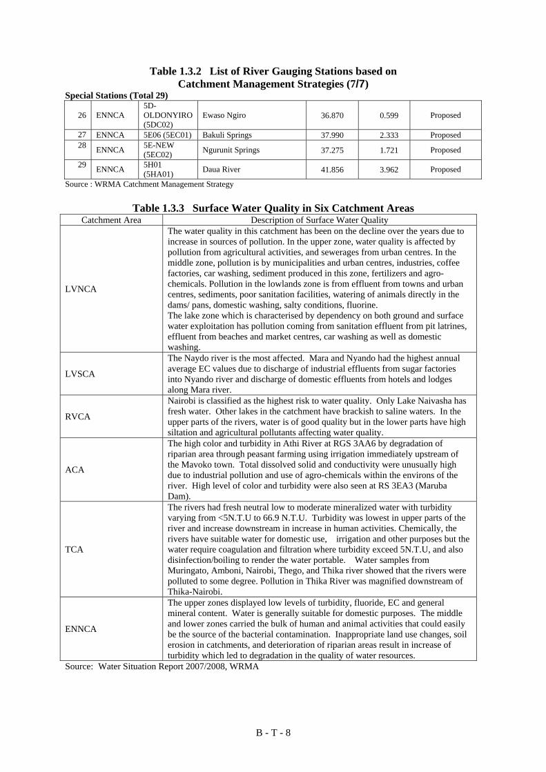
B - T - 8
Table 1.3.2 List of River Gauging Stations based on Catchment Management Strategies (7/7)
Special Stations (Total 29)
26 ENNCA 5D-OLDONYIRO (5DC02)
Ewaso Ngiro 36.870 0.599 Proposed
27 ENNCA 5E06 (5EC01) Bakuli Springs 37.990 2.333 Proposed 28 ENNCA 5E-NEW
(5EC02) Ngurunit Springs 37.275 1.721 Proposed
29 ENNCA 5H01 (5HA01) Daua River 41.856 3.962 Proposed
Source : WRMA Catchment Management Strategy
Table 1.3.3 Surface Water Quality in Six Catchment Areas Catchment Area Description of Surface Water Quality
LVNCA
The water quality in this catchment has been on the decline over the years due to increase in sources of pollution. In the upper zone, water quality is affected by pollution from agricultural activities, and sewerages from urban centres. In the middle zone, pollution is by municipalities and urban centres, industries, coffee factories, car washing, sediment produced in this zone, fertilizers and agro-chemicals. Pollution in the lowlands zone is from effluent from towns and urban centres, sediments, poor sanitation facilities, watering of animals directly in the dams/ pans, domestic washing, salty conditions, fluorine. The lake zone which is characterised by dependency on both ground and surface water exploitation has pollution coming from sanitation effluent from pit latrines, effluent from beaches and market centres, car washing as well as domestic washing.
LVSCA
The Naydo river is the most affected. Mara and Nyando had the highest annual average EC values due to discharge of industrial effluents from sugar factories into Nyando river and discharge of domestic effluents from hotels and lodges along Mara river.
RVCA
Nairobi is classified as the highest risk to water quality. Only Lake Naivasha has fresh water. Other lakes in the catchment have brackish to saline waters. In the upper parts of the rivers, water is of good quality but in the lower parts have high siltation and agricultural pollutants affecting water quality.
ACA
The high color and turbidity in Athi River at RGS 3AA6 by degradation of riparian area through peasant farming using irrigation immediately upstream of the Mavoko town. Total dissolved solid and conductivity were unusually high due to industrial pollution and use of agro-chemicals within the environs of the river. High level of color and turbidity were also seen at RS 3EA3 (Maruba Dam).
TCA
The rivers had fresh neutral low to moderate mineralized water with turbidity varying from <5N.T.U to 66.9 N.T.U. Turbidity was lowest in upper parts of the river and increase downstream in increase in human activities. Chemically, the rivers have suitable water for domestic use, irrigation and other purposes but the water require coagulation and filtration where turbidity exceed 5N.T.U, and also disinfection/boiling to render the water portable. Water samples from Muringato, Amboni, Nairobi, Thego, and Thika river showed that the rivers were polluted to some degree. Pollution in Thika River was magnified downstream of Thika-Nairobi.
ENNCA
The upper zones displayed low levels of turbidity, fluoride, EC and general mineral content. Water is generally suitable for domestic purposes. The middle and lower zones carried the bulk of human and animal activities that could easily be the source of the bacterial contamination. Inappropriate land use changes, soil erosion in catchments, and deterioration of riparian areas result in increase of turbidity which led to degradation in the quality of water resources.
Source: Water Situation Report 2007/2008, WRMA

B - T - 9
Table 2.1.1 List of Temperature Observation Stations and Data Availability for 1979 - 2010
ID Station ID Station Name Latitude Longitude 1979
1980
1981
1982
1983
1984
1985
1986
1987
1988
1989
1990
1991
1992
1993
1994
1995
1996
1997
1998
1999
2000
2001
2002
2003
2004
2005
2006
2007
2008
2009
2010 Total
Validation
1 8635000 LODWAR METEOROLOGICAL STATION 3.1167 35.6167 78.2%
2 8639000 MOYALE MET. STATION 3.5333 39.0500 68.3%
3 8641000 MANDERA MET STATION 3.9333 41.8667 71.0%
4 8737000 MARSABIT MET STATION 2.3167 37.9833 50.5%
5 8834098 KITALE METEOROLOGICAL STATION 1.0000 34.9833 51.5%
6 8840000 WAJIR MET STATION 1.7500 40.0667 81.6%
7 8934096 KAKAMEGA AGROMET STATION 0.2833 34.7667 60.1%
8 8935115 KAPTAGAT ARMS PLATEAU 0.4500 35.4667 30.6%
9 8935181 ELDORET MET.STATION 0.5333 35.2833 36.3%
10 8937022 NANYUKI MET. STATION 0.0500 37.0333 34.0%
11 8937065 MERU MET.STATION 0.0833 37.6500 53.2%
12 9034025 KISUMU METEOROLOGICAL STATION -0.1000 34.7500 56.0%
13 9034088 KISII MET(NYANZA AG.RES.STATION) -0.6833 34.7833 51.7%
14 9035279 HAIL RESEARCH STATION KERICHO -0.3667 35.2667 56.9%
15 9035318 KABARAK AGROMET STATION -0.1833 35.9833 16.9%
16 9036135 NYANDARUA AGRI. RES. STATION -0.0333 36.3500 54.6%
17 9036261 NAKURU METEOROLOGICAL STATION -0.2667 36.1000 45.0%
18 9036288 WAMBUGU F.T.C (NYERI MET STN) -0.4333 36.9667 52.8%
19 9037202 EMBU MET. STATION -0.5000 37.4500 96.2%
20 9039000 GARISSA MET STATION -0.4833 39.6333 50.3%
21 9135001 NAROK METEOROLOGICAL STATION -1.1000 35.8667 56.9%
22 9136087 NAIROBI EASTLEIGH AERODROME -1.2667 36.8667 18.5%
23 9136130 NAIROBI WILSON AIRPORT -1.3167 36.8167 53.3%
24 9136164 DAGORETTI CORNER MET STATION -1.3000 36.7500 56.3%
25 9136168 J.K.I.A.MET.SATION. -1.3167 36.9167 40.0%
26 9136208 KABETE UNIVERSITY FIELD -1.2500 36.7333 56.7%
27 9137048 NATIONAL HORT.RES.STN. THIKA -1.0167 37.1000 33.4%
28 9137089 KATUMANI EXP. RES. STATION. -1.5833 37.2333 58.9%
29 9237000 MAKINDU MET. STATION -2.2833 37.8333 61.6%
30 9240001 LAMU METEOROLOGICAL STATION -2.2667 40.9000 93.7%
31 9338001 VOI METEOROLOGICAL STATION -3.4000 38.5667 96.2%
32 9339036 MTWAPA AGROMET STATION -3.9333 39.7333 57.4%
33 9340007 MSABAHA AGROMET STATION -3.2667 40.0500 44.8%
34 9340009 MALINDI METEOROLOGICAL STATION -3.2333 40.1000 52.2%
35 9439021 MOMBASA PORT REITZ AIRPORT -4.0333 39.6167 46.3%
SourcSource: Kenya Meteorological DepartmentLegend Annual data availability is more than 90%
80% <= data availability < 90%70% <= data availability < 80%60% <= data availability < 70%50% <= data availability < 60%40% <= data availability < 50%less than 40%
Source: KMD

B - T - 10
Table 2.1.2 List of Rainfall Observation Stations and Those Data Availability for 1979 – 2010 (1/3)
ID Station ID Station Name Latitude Longitude 1979
1980
1981
1982
1983
1984
1985
1986
1987
1988
1989
1990
1991
1992
1993
1994
1995
1996
1997
1998
1999
2000
2001
2002
2003
2004
2005
2006
2007
2008
2009
2010 Total
Validation1 8536001 ILERET POLICE POST 4.3167 36.2333 62.2%
2 8635000 LODWAR METEOROLOGICAL STATION 3.1167 35.6167 98.7%
3 8635002 KALOKAL FISHERIES DEPARTMENT 3.5333 35.8833 65.1%
4 8637002 KALACHA A.I. CHURCH 3.1167 37.4167 71.1%
5 8639000 MOYALE MET. STATION 3.5333 39.0500 99.2%
6 8641000 MANDERA MET STATION 3.9333 41.8667 98.8%
7 8641001 MANDERA RHAMU POLICE POST 3.9333 41.2333 69.3%
8 8735004 KEKORONGO IRRIGATION SCHEME 2.8833 35.4167 50.5%
9 8735005 KAPUTIR IRRIGATION SCHEME 2.1000 35.4667 64.9%
10 8735007 KATILU IRRIGATION SCHEME 2.2500 35.4333 63.3%
11 8737000 MARSABIT MET STATION 2.3167 37.9833 98.6%
12 8739001 GIRIFTU POLICE POST 2.0167 39.7500 67.1%
13 8740000 EL WAK , MANDERA 2.7833 40.9500 63.3%
14 8834098 KITALE METEOROLOGICAL STATION 1.0000 34.9833 98.7%
15 8835031 KAIBUIBICH KAPENGURIA 1.2000 35.2833 87.1%
16 8835039 LEISSA FARM,KITALE 1.1667 35.0333 94.1%
17 8835047 KUNYAO CHIEF'S OFFICE 1.8000 35.0500 67.8%
18 8836000 MARALAL DISTRICT COMMISSIONER 1.1000 36.7000 75.5%
19 8836001 BARAGOI EL BARTA D.O'S OFFICE 1.7833 36.8000 62.7%
20 8840000 WAJIR MET STATION 1.7500 40.0667 98.4%
21 8934008 KITALE GLOUCESTER VALE ESTATE 0.9000 34.9167 93.3%
22 8934016 LUGARI FOREST STATION 0.6667 34.9000 94.8%
23 8934059 OHOLO CHIEF'S CAMP. 0.1833 34.3333 92.8%
24 8934061 MALAVA AGIRIC. STATION. 0.4500 34.8500 91.0%
25 8934096 KAKAMEGA AGROMET STATION 0.2833 34.7667 99.7%
26 8934134 BUNGOMA WATER SUPPLY 0.5833 34.5667 95.9%
27 8934161 ALUPE COTTON RESEARCH STATION 0.4833 34.1333 90.6%
28 8935010 KAPTAGAT FOREST STATION 0.4333 35.5000 80.5%
29 8935014 TAMBACH D.O.'S OFFICE 0.6000 35.5333 85.8%
30 8935104 TAMBACH CHEBIEMIT AGRIC OFFICE 0.8667 35.5000 86.7%
31 8935120 KIBABET ESTATE LTD. 0.1333 35.2833 88.9%
32 8935137 TIMBOROA FOREST STATION 0.0667 35.5333 93.9%
33 8935177 KATIMOK FOREST STATION 0.6000 35.7833 94.6%
34 8935181 ELDORET MET.STATION 0.5333 35.2833 99.2%
35 8935188 KAPKEBEN CHEMONI ESTATE 0.1333 35.1333 94.2%
36 8935200 KIMOSE AGRIC.HOLDING GROUND 0.2500 35.8833 85.6%
37 8936014 MUTARA ESTATE MANAGER'S HOUSE 0.1167 36.6833 82.2%
38 8936049 RUMURUTI OL MYSOR 0.4167 36.6667 93.7%
39 8936060 COLCHECCIO LTD. LAIKIPIA 0.6333 36.8000 83.6%
40 8936067 SNAKE FARM,LAKE BARINGO 0.6333 36.1500 82.8%
source: counted by JICA Study Team with original data from Kenya Meteorological DepartmentLegend Annual data availability is more than 90%
80% <= data availability < 90%70% <= data availability < 80%60% <= data availability < 70%50% <= data availability < 60%40% <= data availability < 50%less than 40%

B - T - 11
Table 2.1.2 List of Rainfall Observation Stations and Those Data Availability for 1979 – 2010 (2/3)
ID Station ID Station Name Latitude Longitude 1979
1980
1981
1982
1983
1984
1985
1986
1987
1988
1989
1990
1991
1992
1993
1994
1995
1996
1997
1998
1999
2000
2001
2002
2003
2004
2005
2006
2007
2008
2009
2010 Total
Validation41 8937002 TIMAU MARANIA 0.0833 37.4500 93.6%
42 8937003 ISIOLO DISTRICT AGRIC.OFFICE 0.3500 37.5833 93.7%
43 8937014 MIKINDURI PRIMARY SCHOOL MERU 0.1167 37.8333 89.5%
44 8937022 NANYUKI MET. STATION 0.0500 37.0333 85.7%
45 8937065 MERU MET.STATION 0.0833 37.6500 98.9%
46 8938000 GARBATULLA POLICE STATION 0.5333 38.5167 76.0%
47 9034025 KISUMU METEOROLOGICAL STATION -0.1000 34.7500 99.7%
48 9034036 BONDO WATER SUPPLY -0.0500 34.2833 90.9%
49 9034059 MACALDER AGRICULTURAL OFFICE -0.9667 34.3000 73.2%
50 9034087 LAMBWE FOREST STATION -0.6500 34.3500 91.2%
51 9034088 KISII MET(NYANZA AG.RES.STATION) -0.6833 34.7833 97.9%
52 9034124 MASAKA APUNDO'S FARM -0.2000 34.9833 94.2%
53 9035001 JAMJI ESTATE (KERICHO) -0.4833 35.1833 50.3%
54 9035002 LONDIANI FOREST STATION -0.1500 35.6000 50.2%
55 9035013 SOTIK MONIERI TEA ESTATE -0.6500 35.0667 92.5%
56 9035117 MARIASHON FOREST STATION -0.3667 35.8167 91.3%
57 9035220 KORU HOMALINE CO. LTD -0.1667 35.2833 93.7%
58 9035265 BOMET WATER SUPPLY -0.7833 35.3500 90.5%
59 9035267 MENENGAI FARM -0.2167 35.9667 95.4%
60 9035274 CHEMELIL SUGAR SCHEME -0.0667 35.1333 93.7%
61 9035279 HAIL RESEARCH STATION KERICHO -0.3667 35.2667 99.2%
62 9036017 NYERI MINISTRY OF WORKS -0.4167 36.9500 87.6%
63 9036025 N. KINANGOP FOREST STATION -0.5833 36.6333 90.5%
64 9036029 GILGIL KWETU FARM -0.3500 36.3000 94.7%
65 9036081 NAIVASHA VET.EXPT. STATION -0.6500 36.4167 93.2%
66 9036135 NYANDARUA AGRI. RES. STATION -0.0333 36.3500 97.9%
67 9036147 ELEMENTAITA,SOYSAMBU ESTATE -0.4667 36.2000 90.0%
68 9036259 GATARE FOREST STATION -0.7167 36.7667 86.8%
69 9036261 NAKURU METEOROLOGICAL STATION -0.2667 36.1000 97.5%
70 9037096 SAGANA FISH CULTURE FARM -0.6667 37.2000 90.3%
71 9037099 KARATINA KAGOCHI -0.3833 37.1500 93.3%
72 9037123 CHOGORIA FOREST STATION -0.2833 37.6167 93.2%
73 9037177 KALABA CHIEF'S OFFICE -0.7500 37.3833 90.1%
74 9037202 EMBU MET. STATION -0.5000 37.4500 99.2%
75 9037210 KAMBURU POWER STATION -0.8000 37.6833 83.8%
76 9038023 MUMONI FOREST RESERVE -0.5333 38.0167 91.4%
77 9039000 GARISSA MET STATION -0.4833 39.6333 97.9%
78 9134011 SOTIK DIV AGRI OFFICE -1.0000 34.8833 75.4%
79 9134025 MIGORI WATER SUPPLY -1.0667 34.4667 67.7%
80 9135001 NAROK METEOROLOGICAL STATION -1.1000 35.8667 98.6%
source: counted by JICA Study Team with original data from Kenya Meteorological DepartmentLegend Annual data availability is more than 90%
80% <= data availability < 90%70% <= data availability < 80%60% <= data availability < 70%50% <= data availability < 60%40% <= data availability < 50%less than 40%
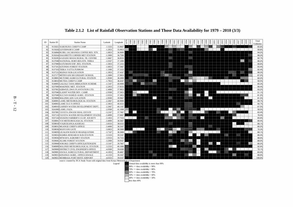
B - T - 12
Table 2.1.2 List of Rainfall Observation Stations and Those Data Availability for 1979 – 2010 (3/3)
ID Station ID Station Name Latitude Longitude 1979
1980
1981
1982
1983
1984
1985
1986
1987
1988
1989
1990
1991
1992
1993
1994
1995
1996
1997
1998
1999
2000
2001
2002
2003
2004
2005
2006
2007
2008
2009
2010 Total
Validation81 9135021 NAROSURA CHIEF'S CAMP -1.5333 35.8667 65.8%
82 9135026 GOVERNOR'S CAMP -1.2833 35.0833 50.8%
83 9136084 RUIRU JACARANDA COFFEE RES. STN. -1.0833 36.9000 94.2%
84 9136164 DAGORETTI CORNER MET STATION -1.3000 36.7500 98.3%
85 9136185 KAJIADO MASAI RURAL TR. CENTRE -1.6667 36.8333 92.7%
86 9137048 NATIONAL HORT.RES.STN. THIKA -1.0167 37.1000 96.2%
87 9137089 KATUMANI EXP. RES. STATION. -1.5833 37.2333 98.8%
88 9137101 KITONDO FOREST STATION -1.6833 37.5667 93.4%
89 9137103 THIKA YATTA FURROW -1.1000 37.3333 92.4%
90 9137131 MANGO SUB-LOCATION -1.3833 37.4167 90.3%
91 9137177 MITINYANI SECONDARY SCHOOL -1.3000 37.9833 87.2%
92 9138001 MUTOMO AGRICULTURAL STATION -1.8500 38.2000 82.2%
93 9138010 MUTHA CHIEF'S CAMP -1.7833 38.4167 50.5%
94 9140005 GALOLE TANA IRRIGATION SCHEME -1.5167 40.0000 65.3%
95 9237000 MAKINDU MET. STATION -2.2833 37.8333 99.4%
96 9237002 KIBWEZI, DWA PLANTATION LTD. -2.4000 37.9833 93.2%
97 9237040 ILASSIT WATER DEV. CAMP. -2.9500 37.5833 51.1%
98 9237049 SULTAN HAMUD AGRIC. STATION -2.0333 37.3833 81.2%
99 9239000 MALINDI ADU LOCATION -2.8500 39.9667 81.5%
100 9240001 LAMU METEOROLOGICAL STATION -2.2667 40.9000 99.7%
101 9240003 LAMU D.O.'S OFFICE -2.3833 40.4333 92.7%
102 9240010 GARSEN WATER DEVELOPMENT DEPT. -2.2667 40.1167 87.5%
103 9241000 LAMU, FAZA -2.0500 41.1000 50.5%
104 9337081 TAVETA ZIWANI SISAL ESTATE -3.2167 37.7667 63.4%
105 9337110 TAVETA WATER DEVELOPMENT STATION -3.4000 37.6667 78.4%
106 9337144 NJUKINI FARMER'S CO.OP. SOCIETY -3.1833 37.7333 65.0%
107 9338001 VOI METEOROLOGICAL STATION -3.4000 38.5667 99.4%
108 9338018 VOI,RUKANGA-KASIGAU -3.8333 38.6333 86.1%
109 9338031 MGANGE CHIEF'S OFFICE -3.4000 38.3167 80.2%
110 9338036 MANYANI GATE -3.0833 38.5000 72.3%
111 9338059 LIUALENI RANCH HEADQUATERS -3.7167 38.3000 66.1%
112 9339016 BAMBA RESEARCH SUB-STATION -3.5333 39.5167 86.4%
113 9339036 MTWAPA AGROMET STATION -3.9333 39.7333 98.9%
114 9339045 JILORE FOREST STATION -3.2000 39.9167 88.0%
115 9339068 SOKOKE CHIEF'S OFFICE,KITENGENI -3.5167 39.7667 80.2%
116 9340009 MALINDI METEOROLOGICAL STATION -3.2333 40.1000 92.9%
117 9439000 DISTRICT CIVIL ENGINEER'S OFFICE -4.0500 39.6500 72.1%
118 9439001 KWALE AGRICULTURAL DEPARTMENT -4.1833 39.4667 83.4%
119 9439015 KINANGO AGRIC. OFFICE KWALE -4.1333 39.3167 86.0%
120 9439021 MOMBASA PORT REITZ AIRPORT -4.0333 39.6167 100.0%
source: counted by JICA Study Team with original data from Kenya Meteorological DepartmentLegend Annual data availability is more than 90%
80% <= data availability < 90%70% <= data availability < 80%60% <= data availability < 70%50% <= data availability < 60%40% <= data availability < 50%less than 40%

B - T - 13
Table 3.2.1 List of Synoptic Stations Used for Calculation ID Station Name Established Selected for
Calculation8635000 Lodwar Meteorological Station 1919 ○ 8639000 Moyale Met. Station 1915 ○ 8641000 Mandera Met Station 1936 ○
8737000 Marsabit Met Station 1918 ○
8834098 Kitale Meteorological Station 1950 8840000 Wajir Met Station 1917 ○ 8934096 Kakamega Agromet Station 1957 8935115 Eldoret International Airport 1997 8935181 Eldoret Met. Station 1972 8937022 Laikipia Air Base 1939 ○ 8937065 Meru Met. Station 1966 9034025 Kisumu Meteorological Station 1938 ○ 9034088 Kisii Met Station 1962 9034103 Suba 2006 9035279 Hail Research Station, Kericho 1963 9036135 Nyahururu Agromet Station 1945 9036261 Nakuru Meteorological Station 1964 9036288 Nyeri Met Station 1968 9037202 Embu Met. Station 1975 9039000 Garissa Met Station 1932 ○
9135001 Narok Meteorological Station 1913 ○
9136087 Moi Airbase, Nairobi 1954 9136130 Wilson Airport, Nairobi 1951 9136164 Dagoretti Corner Met Station 1954 9136168 Jomo Kenyatta International Airport Met Station 1954 9136208 Kabete Agromet Station 1915 Selected 9137048 National Hort. Res. Station, Thika 1941 9137089 Katumani Exp. Res. Station, Machakos 1956 9237000 Makindu Met. Station 1904 Selected 9240001 Lamu Meteorological Station 1906 ○
9338001 Voi Meteorological Station 1904 ○
9339036 Mtwapa Agromet Station 1959 9340007 Msabaha Agromet Station 1956 9340009 Malindi Meteorological Station 1961 9439021 Mombasa Port Reitz Airport 1890 ○
Kangema Total 36 Stations 14 Stations
Note: Observation has not officially stated at KANGEMA Source : KMD

B - T - 14
Table 3.2.2 List of Stations used in NWMP 1992 for Calculation
ID Station Name Selected for Calculation Note
8635000 Lodwar Meteorological Station Synoptic 8639000 Moyale Met. Station Synoptic Synoptic 8934001 Kakamega D C 8934008 Kitale Gloucester Vale Estate Selected 8935018 Kapsabet D.C.'s Office 9034001 Kisii D.C.'s Office 9034004 Kisumu P.C's Office 9035002 Londiani Forest Station 9035003 Kericho District Office 9036002 Naivasha D.O. 9036017 Nyeri Ministry of Works Selected Selected 9036020 Nakuru Railway Station Selected Selected 9135001 Narok Meteorological Station Synoptic Synoptic 9136020 Ihothia Farm, Limuru 9136028 Kiambu District Office 9137002 Sassa Coffee, Kenya Canners 9137010 Machakos District Office 9237000 Makindu Met. Station Synoptic Synoptic 9240001 Lamu Meteorological Station Synoptic Synoptic 9338001 Voi Meteorological Station Synoptic Synoptic 9340000 Malindi District Office 9439001 Kwale Agricultural Department 9439002 Mombasa Old Observatory 9439045 Mombasa Shimanzi Water Division
Total 22 Stations 3 Stations
Source: NWMP1992

B - T - 15
Table 4.3.1 List of GCMs and Developers No Model Name Developers 1 bcc-cm1 Beijing Climate Center, China 2 bccr-bcm2.0 Bjerknes Centre for Climate Research, Norway 3 cccma_cgcm3_1 Canadian Centre for Climate Modelling and Analysis, Victoria, BC, Canada 4 cccma_cgcm3_1_t63 Canadian Centre for Climate Modelling and Analysis, Victoria, BC, Canada 5 cnrm_cm3 Centre National de Researches Meteorologiques, Meteo-France, Toulouse, France 6 csiro_mk3_0 CSIRO Atmospheric Research, Melbourne, Australia 7 csiro_mk3_5 CSIRO Atmospheric Research, Melbourne, Australia
8 gfdl_cm2_0 US Dept of Commerce / NOAA / Geophysical Fluid Dynamics Laboratory, Princeton, NJ, USA
9 gfdl_cm2_1 US Dept of Commerce / NOAA / Geophysical Fluid Dynamics Laboratory, Princeton, NJ, USA
10 giss_aom NASA/Goddard Institute for Space Studies, New York, USA 11 giss_model_e_h NASA/GISS (Goddard Institute for Space Studies)New York, NY 12 giss_model_e_r NASA/GISS (Goddard Institute for Space Studies)New York, NY
13 iap_fgoals1_0_g LASG, Institute of Atmospheric Physics, P.O. Box 9804, Beijing 100029, P.R. China
14 ingv_echam4 National Institute of Geophysics and Volcanology, Bologna, Italy 15 inmcm3_0 Institute for Numerical Mathematics, Moscow, Russia 16 ipsl_cm4 Institut Pierre Simon Laplace, Paris, France
17 miroc3_2_hires Center for Climate System Research, Tokyo, Japan / National Institute for Environmental Studies, Ibaraki, Japan / Frontier Research Center for Global Change, Kanagawa, Japan
18 miroc3_2_medres Center for Climate System Research, Tokyo, Japan / National Institute for Environmental Studies, Ibaraki, Japan / Frontier Research Center for Global Change, Kanagawa, Japan
19 miub_echo_g University of Bonn, Bonn, Germany, Meteorological Research Institute, Seoul, Korea
20 mpi_echam5 Max Planck Institute for Meteorology, Hamburg, Germany 21 mri_cgcm2_3_2a Meteorological Research Institute, Tsukuba, Ibaraki, Japan 22 ncar_ccsm3_0 National Center for Atmospheric Research, Boulder, CO, USA 23 ncar_pcm1 National Center for Atmospheric Research, Boulder, CO, USA 24 ukmo_hadcm3 Hadley Centre for climate Prediction and Research/Met office, UK 25 ukmo_hadgem1 Hadley Centre for climate Prediction and Research/Met office, UK
Source: CMIP3 CMIP3 Climate Model Documentation, References, and Links (http://www-pcmdi.llnl.gov/ipcc/model_documentation/ipcc_model_documentation.php)

B - T - 16
Table 4.4.1 Monthly and Daily Data Availability of GCMs No Model Name Developers Monthly Daily - bcc-cm1 Beijing Climate Center, China missing missing - bccr-bcm2.0 Bjerknes Centre for Climate Research, Norway missing
1 cccma_cgcm3_1 Canadian Centre for Climate Modelling and Analysis, Victoria, BC, Canada
2 cccma_cgcm3_1_t63 Canadian Centre for Climate Modelling and Analysis, Victoria, BC, Canada
3 cnrm_cm3 Centre National de Researches Meteorologiques, Meteo-France, Toulouse, France
4 csiro_mk3_0 CSIRO Atmospheric Research, Melbourne, Australia 5 csiro_mk3_5 CSIRO Atmospheric Research, Melbourne, Australia
6 gfdl_cm2_0 US Dept of Commerce / NOAA / Geophysical Fluid Dynamics Laboratory, Princeton, NJ, USA
7 gfdl_cm2_1 US Dept of Commerce / NOAA / Geophysical Fluid Dynamics Laboratory, Princeton, NJ, USA
8 giss_aom NASA/Goddard Institute for Space Studies, New York, USA - giss_model_e_h NASA/GISS (Goddard Institute for Space Studies)New York, NY missing 9 giss_model_e_r NASA/GISS (Goddard Institute for Space Studies)New York, NY
10 iap_fgoals1_0_g LASG, Institute of Atmospheric Physics, P.O. Box 9804, Beijing 100029, P.R. China
11 ingv_echam4 National Institute of Geophysics and Volcanology, Bologna, Italy inmcm3_0 Institute for Numerical Mathematics, Moscow, Russia missing
12 ipsl_cm4 Institut Pierre Simon Laplace, Paris, France
13 miroc3_2_hires Center for Climate System Research, Tokyo, Japan / National Institute for Environmental Studies, Ibaraki, Japan / Frontier Research Center for Global Change, Kanagawa, Japan
14 miroc3_2_medres Center for Climate System Research, Tokyo, Japan / National Institute for Environmental Studies, Ibaraki, Japan / Frontier Research Center for Global Change, Kanagawa, Japan
15 miub_echo_g University of Bonn, Bonn, Germany, Meteorological Research Institute, Seoul, Korea
16 mpi_echam5 Max Planck Institute for Meteorology, Hamburg, Germany 17 mri_cgcm2_3_2a Meteorological Research Institute, Tsukuba, Ibaraki, Japan - ncar_ccsm3_0 National Center for Atmospheric Research, Boulder, CO, USA missing - ncar_pcm1 National Center for Atmospheric Research, Boulder, CO, USA missing missing - ukmo_hadcm3 Hadley Centre for climate Prediction and Research/Met office, UK missing - ukmo_hadgem1 Hadley Centre for climate Prediction and Research/Met office, UK missing
Source: CMIP3 Climate Model Documentation, References, and Links (http://www-pcmdi.llnl.gov/ipcc/model_documentation/ipcc_model_documentation.php)

B - T - 17
Table 4.4.2 Precipitation for 20 years Climatology by Spatial Correlation: Observed Present (Reanalysis) and Simulated Present (20C3M)
GCM Jan Feb Mar Apr May Jun Jul Aug Sep Oct Nov Deccccma_cgcm3_1 0.88 0.92 0.88 0.45 0.69 0.88 0.91 0.92 0.91 0.86 0.80 0.64 cccma_cgcm3_1_t63 0.85 0.90 0.85 0.47 0.76 0.93 0.93 0.90 0.95 0.88 0.78 0.74 cnrm_cm3 0.92 0.93 0.88 0.69 0.81 0.71 0.76 0.90 0.88 0.72 0.75 0.85 csiro_mk3_0 0.91 0.91 0.82 0.43 0.76 0.92 0.96 0.96 0.95 0.75 0.76 0.84 csiro_mk3_5 0.89 0.91 0.89 0.57 0.74 0.93 0.95 0.95 0.95 0.84 0.81 0.81 gfdl_cm2_0 0.97 0.95 0.91 0.66 0.80 0.84 0.92 0.93 0.91 0.90 0.83 0.94 gfdl_cm2_1 0.93 0.91 0.86 0.47 0.72 0.73 0.82 0.81 0.82 0.75 0.78 0.85 giss_aom 0.57 0.56 0.71 0.46 0.43 0.14 0.40 0.55 0.42 0.21 0.21 0.45 giss_model_e_r 0.72 0.59 0.70 0.45 0.49 0.29 0.34 0.49 0.46 0.31 0.39 0.65 iap_fgoals1_0_g 0.88 0.89 0.88 0.65 0.77 0.44 0.76 0.88 0.90 0.83 0.82 0.91 ingv_echam4 0.89 0.85 0.94 0.57 0.83 0.92 0.92 0.84 0.93 0.81 0.74 0.84 ipsl_cm4 0.89 0.92 0.88 0.45 0.67 0.74 0.88 0.90 0.88 0.81 0.78 0.86 miroc3_2_hires 0.86 0.91 0.88 0.71 0.70 0.87 0.87 0.93 0.93 0.81 0.77 0.82 miroc3_2_medres 0.96 0.94 0.91 0.49 0.52 0.78 0.78 0.80 0.85 0.90 0.83 0.94 miub_echo_g 0.84 0.88 0.88 0.35 0.56 0.73 0.91 0.91 0.94 0.83 0.60 0.73 mpi_echam5 0.92 0.90 0.86 0.53 0.79 0.91 0.95 0.97 0.95 0.82 0.77 0.77 mri_cgcm2_3_2a 0.82 0.87 0.84 0.58 0.59 0.76 0.76 0.84 0.91 0.77 0.69 0.74
Source: Evaluated by JICA Study Team with the data obtained from Data Integration and Analysis System (DIAS) dataset, and The Phase 3 of Coupled Model Intercomparison Project (CMIP3) multi-model dataset.
Table 4.4.3 Precipitation for 20 years Climatology by RMSE: Observed Present (Reanalysis) and Simulated Present (20C3M)
(Unit: mm/day) GCM Jan Feb Mar Apr May Jun Jul Aug Sep Oct Nov Dec
cccma_cgcm3_1 2.54 1.89 1.77 2.33 1.67 1.48 1.39 1.29 1.65 2.15 3.02 4.64 cccma_cgcm3_1_t63 3.12 2.29 1.77 2.50 1.78 1.52 1.34 1.58 1.78 2.48 4.02 4.64 cnrm_cm3 2.77 1.29 1.09 1.88 2.82 2.51 1.97 1.79 1.91 2.84 3.86 3.10 csiro_mk3_0 1.14 1.00 1.38 2.31 1.57 0.88 0.69 0.80 1.23 2.04 2.24 1.66 csiro_mk3_5 1.12 0.98 1.21 2.35 2.05 0.85 0.79 0.94 1.48 2.37 2.93 2.13 gfdl_cm2_0 1.39 1.13 1.40 2.16 1.87 1.29 0.93 0.99 1.20 1.99 2.62 2.05 gfdl_cm2_1 1.31 0.90 1.48 2.35 1.88 1.34 1.56 1.66 1.35 1.84 2.90 2.40 giss_aom 4.22 3.60 2.02 1.91 1.67 2.52 2.08 2.02 2.25 2.79 3.86 4.25 giss_model_e_r 2.69 3.26 2.87 2.40 2.44 2.64 2.32 2.18 2.11 2.83 3.61 3.40 iap_fgoals1_0_g 2.51 2.21 1.80 1.91 1.55 2.58 1.42 1.20 1.47 2.04 2.39 2.01 ingv_echam4 1.13 1.26 1.11 1.75 1.56 0.88 0.89 1.30 1.05 1.62 1.52 1.26 ipsl_cm4 3.01 2.09 1.36 2.30 1.55 1.27 1.50 1.39 1.07 1.49 2.32 3.02 miroc3_2_hires 2.33 1.62 1.90 1.87 2.11 1.97 2.27 2.00 2.18 2.18 3.11 2.38 miroc3_2_medres 1.66 1.72 1.07 1.86 1.74 1.72 2.12 2.71 2.84 1.14 1.14 0.83 miub_echo_g 1.52 1.20 1.04 2.11 2.62 1.60 0.93 1.08 0.81 1.30 2.15 2.35 mpi_echam5 0.94 0.91 1.48 2.14 1.61 1.09 1.03 1.10 0.70 1.40 1.62 1.78 mri_cgcm2_3_2a 2.03 2.01 2.08 2.83 2.56 2.15 2.07 1.78 2.35 3.23 3.19 2.74
Note: RMSE (Root-mean-square error) Source: Evaluated by JICA Study Team with the data obtained from Data Integration and Analysis System (DIAS) dataset,
and The Phase 3 of Coupled Model Intercomparison Project (CMIP3) multi-model dataset.
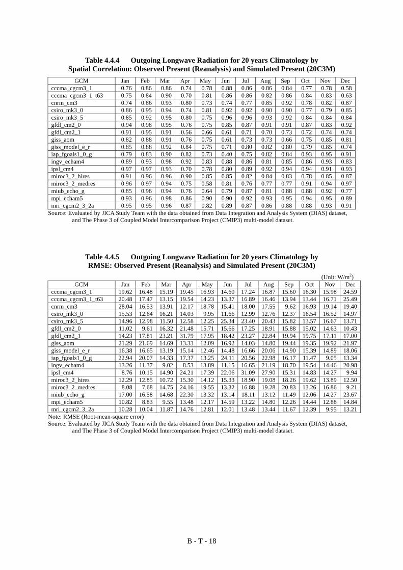
B - T - 18
Table 4.4.4 Outgoing Longwave Radiation for 20 years Climatology by Spatial Correlation: Observed Present (Reanalysis) and Simulated Present (20C3M)
GCM Jan Feb Mar Apr May Jun Jul Aug Sep Oct Nov Deccccma_cgcm3_1 0.76 0.86 0.86 0.74 0.78 0.88 0.86 0.86 0.84 0.77 0.78 0.58 cccma_cgcm3_1_t63 0.75 0.84 0.90 0.70 0.81 0.86 0.86 0.82 0.86 0.84 0.83 0.63 cnrm_cm3 0.74 0.86 0.93 0.80 0.73 0.74 0.77 0.85 0.92 0.78 0.82 0.87 csiro_mk3_0 0.86 0.95 0.94 0.74 0.81 0.92 0.92 0.90 0.90 0.77 0.79 0.85 csiro_mk3_5 0.85 0.92 0.95 0.80 0.75 0.96 0.96 0.93 0.92 0.84 0.84 0.84 gfdl_cm2_0 0.94 0.98 0.95 0.76 0.75 0.85 0.87 0.91 0.91 0.87 0.83 0.92 gfdl_cm2_1 0.91 0.95 0.91 0.56 0.66 0.61 0.71 0.70 0.73 0.72 0.74 0.74 giss_aom 0.82 0.88 0.91 0.76 0.75 0.61 0.73 0.73 0.66 0.75 0.85 0.81 giss_model_e_r 0.85 0.88 0.92 0.84 0.75 0.71 0.80 0.82 0.80 0.79 0.85 0.74 iap_fgoals1_0_g 0.79 0.83 0.90 0.82 0.73 0.40 0.75 0.82 0.84 0.93 0.95 0.91 ingv_echam4 0.89 0.93 0.98 0.92 0.83 0.88 0.86 0.81 0.85 0.86 0.93 0.83 ipsl_cm4 0.97 0.97 0.93 0.70 0.78 0.80 0.89 0.92 0.94 0.94 0.91 0.93 miroc3_2_hires 0.91 0.96 0.96 0.90 0.85 0.85 0.82 0.84 0.83 0.78 0.85 0.87 miroc3_2_medres 0.96 0.97 0.94 0.75 0.58 0.81 0.76 0.77 0.77 0.91 0.94 0.97 miub_echo_g 0.85 0.96 0.94 0.76 0.64 0.79 0.87 0.81 0.88 0.88 0.92 0.77 mpi_echam5 0.93 0.96 0.98 0.86 0.90 0.90 0.92 0.93 0.95 0.94 0.95 0.89 mri_cgcm2_3_2a 0.95 0.95 0.96 0.87 0.82 0.89 0.87 0.86 0.88 0.88 0.93 0.91
Source: Evaluated by JICA Study Team with the data obtained from Data Integration and Analysis System (DIAS) dataset, and The Phase 3 of Coupled Model Intercomparison Project (CMIP3) multi-model dataset.
Table 4.4.5 Outgoing Longwave Radiation for 20 years Climatology by RMSE: Observed Present (Reanalysis) and Simulated Present (20C3M)
(Unit: W/m2) GCM Jan Feb Mar Apr May Jun Jul Aug Sep Oct Nov Dec
cccma_cgcm3_1 19.62 16.48 15.19 19.45 16.93 14.60 17.24 16.87 15.60 16.30 15.98 24.59 cccma_cgcm3_1_t63 20.48 17.47 13.15 19.54 14.23 13.37 16.89 16.46 13.94 13.44 16.71 25.49 cnrm_cm3 28.04 16.53 13.91 12.17 18.78 15.41 18.00 17.55 9.62 16.93 19.14 19.40 csiro_mk3_0 15.53 12.64 16.21 14.03 9.95 11.66 12.99 12.76 12.37 16.54 16.52 14.97 csiro_mk3_5 14.96 12.98 11.50 12.58 12.25 25.34 23.40 20.43 15.82 13.57 16.67 13.71 gfdl_cm2_0 11.02 9.61 16.32 21.48 15.71 15.66 17.25 18.91 15.88 15.02 14.63 10.43 gfdl_cm2_1 14.23 17.81 23.21 31.79 17.95 18.42 23.27 22.84 19.94 19.75 17.11 17.00 giss_aom 21.29 21.69 14.69 13.33 12.09 16.92 14.03 14.80 19.44 19.35 19.92 21.97 giss_model_e_r 16.38 16.65 13.19 15.14 12.46 14.48 16.66 20.06 14.90 15.39 14.89 18.06 iap_fgoals1_0_g 22.94 20.07 14.33 17.37 13.25 24.11 20.56 22.98 16.17 11.47 9.05 13.34 ingv_echam4 13.26 11.37 9.02 8.53 13.89 11.15 16.65 21.19 18.70 19.54 14.46 20.98 ipsl_cm4 8.76 10.15 14.90 24.21 17.39 22.06 31.09 27.90 15.31 14.83 14.27 9.94 miroc3_2_hires 12.29 12.85 10.72 15.30 14.12 15.33 18.90 19.08 18.26 19.62 13.89 12.50 miroc3_2_medres 8.08 7.68 14.75 24.16 19.55 13.32 16.88 19.28 20.83 13.26 16.86 9.21 miub_echo_g 17.00 16.58 14.68 22.30 13.32 13.14 18.11 13.12 11.49 12.06 14.27 23.67 mpi_echam5 10.82 8.83 9.55 13.48 12.17 14.59 13.22 14.80 12.26 14.44 12.88 14.84 mri_cgcm2_3_2a 10.28 10.04 11.87 14.76 12.81 12.01 13.48 13.44 11.67 12.39 9.95 13.21
Note: RMSE (Root-mean-square error) Source: Evaluated by JICA Study Team with the data obtained from Data Integration and Analysis System (DIAS) dataset,
and The Phase 3 of Coupled Model Intercomparison Project (CMIP3) multi-model dataset.

B - T - 19
Table 4.4.6 Sea Level Pressure for 20 years Climatology by Spatial Correlation: Observed Present (Reanalysis) and Simulated Present (20C3M)
GCM Jan Feb Mar Apr May Jun Jul Aug Sep Oct Nov Deccccma_cgcm3_1 0.38 0.43 0.49 0.62 0.81 0.87 0.89 0.88 0.83 0.66 0.40 0.38 cccma_cgcm3_1_t63 0.36 0.42 0.48 0.59 0.82 0.90 0.93 0.91 0.85 0.66 0.36 0.25 cnrm_cm3 0.65 0.81 0.85 0.79 0.74 0.83 0.91 0.93 0.92 0.85 0.45 0.51 csiro_mk3_0 0.52 0.49 0.53 0.66 0.84 0.89 0.93 0.93 0.84 0.73 0.72 0.63 csiro_mk3_5 0.54 0.45 0.54 0.66 0.83 0.83 0.89 0.91 0.85 0.76 0.73 0.63 gfdl_cm2_0 0.67 0.59 0.59 0.66 0.79 0.83 0.86 0.86 0.80 0.69 0.70 0.73 gfdl_cm2_1 0.64 0.49 0.48 0.56 0.81 0.88 0.85 0.84 0.81 0.73 0.73 0.75 giss_aom 0.77 0.69 0.75 0.76 0.81 0.90 0.92 0.90 0.84 0.77 0.77 0.80 giss_model_e_r 0.36 0.29 0.40 0.44 0.56 0.71 0.75 0.72 0.67 0.55 0.48 0.45 iap_fgoals1_0_g 0.82 0.75 0.80 0.83 0.84 0.84 0.91 0.91 0.89 0.83 0.81 0.86 ingv_echam4 0.49 0.72 0.92 0.95 0.79 0.87 0.83 0.78 0.77 0.40 0.11 0.20 ipsl_cm4 0.65 0.59 0.59 0.64 0.77 0.84 0.85 0.83 0.75 0.70 0.70 0.70 miroc3_2_hires 0.83 0.81 0.87 0.91 0.94 0.95 0.95 0.94 0.92 0.92 0.95 0.91 miroc3_2_medres 0.74 0.78 0.87 0.90 0.91 0.91 0.89 0.84 0.79 0.77 0.85 0.77 miub_echo_g 0.48 0.70 0.79 0.86 0.79 0.88 0.92 0.89 0.86 0.67 0.07 0.27 mpi_echam5 0.91 0.92 0.93 0.97 0.97 0.97 0.97 0.96 0.94 0.92 0.85 0.88 mri_cgcm2_3_2a 0.86 0.87 0.87 0.89 0.92 0.92 0.92 0.91 0.89 0.78 0.82 0.81
Source: Evaluated by JICA Study Team with the data obtained from Data Integration and Analysis System (DIAS) dataset, and The Phase 3 of Coupled Model Intercomparison Project (CMIP3) multi-model dataset.
Table 4.4.7 Sea Level Pressure for 20 years Climatology by RMSE: Observed Present (Reanalysis) and Simulated Present (20C3M)
(Unit: hPa) GCM Jan Feb Mar Apr May Jun Jul Aug Sep Oct Nov Dec
cccma_cgcm3_1 1.73 2.32 1.97 1.75 1.23 1.52 1.84 2.04 1.88 1.65 1.47 1.58 cccma_cgcm3_1_t63 1.56 1.91 1.87 1.78 1.17 1.37 1.47 1.66 1.51 1.69 1.81 1.55 cnrm_cm3 2.21 1.92 1.40 1.04 1.38 1.56 1.50 1.08 1.04 0.69 1.24 1.80 csiro_mk3_0 1.54 1.59 1.68 1.46 1.00 0.94 0.88 1.07 1.09 1.07 1.07 1.23 csiro_mk3_5 1.45 1.91 1.98 2.10 1.16 1.27 1.33 1.32 1.20 0.96 0.76 1.19 gfdl_cm2_0 1.13 1.49 1.58 1.68 1.77 2.02 2.70 2.67 1.93 1.42 0.80 0.76 gfdl_cm2_1 1.80 2.65 2.65 3.05 2.63 2.13 2.40 2.44 2.16 1.99 1.60 1.23 giss_aom 1.03 1.11 1.03 1.21 1.83 2.53 3.04 3.79 3.51 2.42 1.47 1.26 giss_model_e_r 5.08 5.58 5.27 5.24 5.73 6.06 6.00 6.49 6.34 5.73 5.03 4.98 iap_fgoals1_0_g 0.79 0.90 0.85 1.01 1.42 2.07 1.77 2.00 1.77 0.82 0.60 0.59 ingv_echam4 1.86 1.75 2.22 2.58 2.43 2.44 2.36 2.31 2.20 2.52 2.60 2.43 ipsl_cm4 2.12 2.37 2.19 2.08 2.24 2.46 2.64 2.86 2.73 1.95 1.55 1.63 miroc3_2_hires 2.40 2.19 1.72 1.40 1.37 1.29 1.04 1.08 1.23 1.62 1.55 1.71 miroc3_2_medres 0.85 0.82 0.77 0.85 1.16 1.17 1.27 1.47 1.20 0.75 0.63 0.72 miub_echo_g 1.24 1.09 1.03 0.79 1.18 1.05 0.83 0.93 1.19 1.27 1.62 1.47 mpi_echam5 0.54 0.56 0.62 0.61 0.56 0.58 0.52 0.82 0.70 0.65 0.73 0.57 mri_cgcm2_3_2a 0.61 0.81 0.94 0.87 0.85 0.89 1.21 1.46 1.07 0.98 0.83 0.64
Note: RMSE (Root-mean-square error) Source: Evaluated by JICA Study Team with the data obtained from Data Integration and Analysis System (DIAS) dataset,
and The Phase 3 of Coupled Model Intercomparison Project (CMIP3) multi-model dataset.

B - T - 20
Table 4.4.8 Surface Air Temperature for 20 years Climatology by Spatial Correlation : Observed Present (Reanalysis) and Simulated Present (20C3M)
GCM Jan Feb Mar Apr May Jun Jul Aug Sep Oct Nov Deccccma_cgcm3_1 0.92 0.90 0.90 0.89 0.88 0.84 0.84 0.82 0.79 0.79 0.88 0.92 cccma_cgcm3_1_t63 0.96 0.95 0.94 0.89 0.90 0.90 0.91 0.90 0.88 0.88 0.93 0.95 cnrm_cm3 0.87 0.93 0.96 0.96 0.92 0.87 0.85 0.85 0.91 0.94 0.92 0.88 csiro_mk3_0 0.89 0.90 0.91 0.92 0.92 0.93 0.92 0.92 0.93 0.91 0.92 0.92 csiro_mk3_5 0.84 0.80 0.86 0.89 0.91 0.88 0.86 0.84 0.83 0.87 0.93 0.92 gfdl_cm2_0 0.93 0.92 0.90 0.88 0.85 0.83 0.85 0.85 0.81 0.84 0.87 0.90 gfdl_cm2_1 0.92 0.89 0.85 0.81 0.85 0.87 0.89 0.87 0.82 0.82 0.86 0.89 giss_aom 0.88 0.89 0.93 0.94 0.91 0.87 0.82 0.74 0.74 0.81 0.86 0.88 giss_model_e_r 0.86 0.84 0.89 0.91 0.87 0.83 0.81 0.69 0.62 0.68 0.79 0.86 iap_fgoals1_0_g 0.68 0.68 0.70 0.66 0.69 0.53 0.41 0.33 0.38 0.48 0.65 0.70 ingv_echam4 0.88 0.85 0.89 0.90 0.89 0.84 0.80 0.81 0.84 0.88 0.91 0.91 ipsl_cm4 0.89 0.89 0.91 0.93 0.91 0.87 0.80 0.72 0.81 0.87 0.91 0.91 miroc3_2_hires 0.91 0.93 0.95 0.97 0.95 0.92 0.90 0.89 0.91 0.93 0.96 0.94 miroc3_2_medres 0.83 0.83 0.89 0.89 0.88 0.85 0.81 0.75 0.79 0.83 0.89 0.87 miub_echo_g 0.90 0.90 0.91 0.92 0.90 0.87 0.88 0.81 0.80 0.85 0.87 0.89 mpi_echam5 0.97 0.97 0.97 0.95 0.93 0.92 0.92 0.91 0.90 0.93 0.94 0.97 mri_cgcm2_3_2a 0.85 0.85 0.88 0.89 0.87 0.83 0.80 0.77 0.80 0.80 0.85 0.88
Source: Evaluated by JICA Study Team with the data obtained from Data Integration and Analysis System (DIAS) dataset, and The Phase 3 of Coupled Model Intercomparison Project (CMIP3) multi-model dataset.
Table 4.4.9 Surface Air Temperature for 20 years Climatology by RMSE: Observed Present (Reanalysis) and Simulated Present (20C3M)
(Unit: °C) GCM Jan Feb Mar Apr May Jun Jul Aug Sep Oct Nov Dec
cccma_cgcm3_1 1.91 2.66 2.80 2.92 2.92 3.26 3.18 3.17 3.58 3.30 2.38 1.51 cccma_cgcm3_1_t63 1.14 1.53 2.03 2.54 2.37 2.51 2.29 2.13 2.46 2.35 1.54 1.05 cnrm_cm3 2.24 1.76 1.20 1.05 1.39 1.95 1.85 1.45 1.22 1.05 1.14 1.84 csiro_mk3_0 1.57 1.75 2.26 2.59 1.87 2.07 2.28 2.21 2.27 2.05 1.58 1.51 csiro_mk3_5 4.39 4.86 5.33 5.67 5.08 5.70 5.77 5.57 5.62 5.05 4.21 3.96 gfdl_cm2_0 1.36 1.32 1.79 2.20 2.14 2.20 2.33 2.35 2.50 2.12 1.81 1.91 gfdl_cm2_1 1.33 1.82 2.57 3.17 2.37 1.87 2.35 2.80 2.88 2.43 1.64 1.69 giss_aom 1.63 1.58 1.60 1.94 2.02 2.12 2.71 3.12 2.93 2.39 1.87 1.63 giss_model_e_r 2.04 2.22 1.99 2.25 2.47 2.69 3.21 3.68 3.64 2.93 2.28 1.89 iap_fgoals1_0_g 5.37 6.15 6.40 7.00 5.28 5.35 7.27 8.17 8.22 7.01 5.04 4.44 ingv_echam4 2.73 3.54 4.01 4.04 3.32 3.80 3.86 3.57 3.49 2.91 2.52 2.23 ipsl_cm4 2.69 2.90 3.30 3.67 3.53 3.60 3.89 3.84 3.62 3.43 3.02 2.63 miroc3_2_hires 1.40 1.39 1.60 1.88 1.72 1.59 1.52 1.56 1.61 1.65 1.10 1.16 miroc3_2_medres 2.07 1.88 1.63 1.77 1.78 2.07 2.06 1.90 1.63 1.52 1.28 1.77 miub_echo_g 1.43 1.41 1.52 1.87 1.67 1.73 1.92 1.95 1.97 1.80 1.55 1.51 mpi_echam5 1.75 1.75 2.49 3.45 3.37 3.00 2.91 3.13 3.30 3.00 2.65 2.01 mri_cgcm2_3_2a 2.12 2.13 2.41 2.64 2.60 2.36 2.16 2.09 2.27 2.49 2.35 2.02
Note: RMSE (Root-mean-square error) Source: Evaluated by JICA Study Team with the data obtained from Data Integration and Analysis System (DIAS) dataset,
and The Phase 3 of Coupled Model Intercomparison Project (CMIP3) multi-model dataset.

B - T - 21
Table 4.4.10 Selection of GCMs Used for Calculation GCMs Correlation RMSE Selected for
Calculation No. Name P Olr SLP TAS P Olr SLP TAS 1 cccma_cgcm3_1 Selected 2 cccma_cgcm3_1_t63 Selected 3 cnrm_cm3 Selected 4 csiro_mk3_0 Selected 5 csiro_mk3_5 1 6 gfdl_cm2_0 Selected 7 gfdl_cm2_1 Selected 8 giss_aom 1 9 giss_model_e_r 1 1 10 iap_fgoals1_0_g 1 1 1 11 ingv_echam4 1 12 ipsl_cm4 Selected 13 miroc3_2_hires Selected 14 miroc3_2_medres Selected 15 miub_echo_g 1 16 mpi_echam5 Selected 17 mri_cgcm2_3_2a Selected
Note: In the RMSE and Correlation, the cells inscribed “1” means the model abandoned through the evaluation. RMSE (Root-mean-square error) P : Precipitation Olr :Outgoing Longwave Radiation SLP :Sea Level Pressure TAS :Surface Air Tempreture
Source: Evaluated by JICA Study Team with the data obtained from Data Integration and Analysis System (DIAS) dataset, and The Phase 3 of Coupled Model Intercomparison Project (CMIP3) multi-model dataset.

B - T - 22
Catchment Station Code Station Name Latitude Longitude 1980
1981
1982
1983
1984
1985
1986
1987
1988
1989
1990
1991
1992
1993
1994
1995
1996
1997
1998
1999
2000
2001
2002
2003
2004
2005
2006
2007
2008
2009 Total
AvailabilitySelected forCalibration
LVN 1AD02 Malakisi 0.6250 34.3419 100% 100% 97% 70% 79% 65% 83% 97% 89% 80% 75% 67% 0% 0% 50% 82% 0% 0% 0% 0% 0% 0% 0% 0% 33% 26% 10% 0% 0% 0% 40.1%LVN 1AH01 Sio 0.3875 34.1417 98% 98% 90% 99% 99% 99% 66% 99% 100% 100% 100% 99% 99% 0% 99% 100% 99% 92% 0% 100% 41% 100% 100% 58% 33% 50% 91% 71% 0% 0% 76.0%
LVN 1BD02 Large Zoia 0.7611 35.0611 100% 91% 95% 70% 100% 100% 100% 100% 67% 78% 58% 37% 78% 98% 58% 0% 0% 0% 0% 80% 97% 95% 100% 91% 0% 0% 0% 0% 0% 0% 56.4%
LVN 1BG07 Rongai 0.7740 34.9250 98% 96% 93% 100% 100% 100% 79% 86% 86% 85% 85% 57% 81% 84% 75% 82% 33% 0% 0% 96% 99% 92% 91% 100% 8% 76% 100% 33% 33% 25% 72.4%
LVN 1CE01 Kipkaren 0.6083 34.9653 82% 81% 80% 66% 70% 49% 0% 0% 0% 0% 0% 0% 0% 0% 0% 0% 0% 0% 0% 100% 98% 33% 17% 100% 92% 50% 25% 10% 0% 0% 31.8%LVN 1EE01 Nzoia 0.1780 34.2250 100% 98% 100% 97% 99% 80% 0% 0% 60% 18% 55% 41% 51% 11% 15% 0% 0% 0% 0% 0% 0% 0% 0% 0% 0% 0% 0% 0% 0% 0% 27.5%LVN 1EF01 Nzoia at Ruambwa 0.1236 34.0903 99% 100% 100% 100% 67% 75% 100% 100% 83% 0% 89% 92% 100% 100% 100% 100% 100% 99% 100% 100% 100% 100% 100% 71% 0% 54% 100% 71% 0% 0% 80.0%
LVN 1EG02 Wuoroya 0.1500 34.2431 83% 85% 80% 74% 69% 78% 74% 82% 42% 62% 68% 71% 45% 87% 95% 99% 100% 53% 82% 50% 9% 4% 0% 0% 0% 0% 0% 0% 0% 0% 49.8%
LVN 1FC01 Kimondi 0.2000 35.0486 91% 62% 98% 97% 100% 92% 100% 100% 100% 99% 100% 100% 100% 100% 67% 0% 0% 0% 0% 0% 0% 0% 0% 0% 0% 50% 99% 67% 25% 0% 54.8%LVN 1FE01 Yala 0.1330 34.5750 100% 100% 100% 100% 100% 100% 100% 100% 100% 100% 83% 67% 83% 50% 100% 66% 67% 100% 16% 0% 0% 0% 0% 0% 0% 0% 0% 0% 0% 0% 54.4%LVN 1FG01 Yala 0.0861 34.5583 100% 85% 82% 86% 96% 99% 99% 99% 95% 98% 100% 78% 59% 64% 70% 70% 41% 71% 71% 71% 71% 12% 0% 0% 0% 0% 0% 0% 0% 0% 57.2%
LVN 1FG02 Yala 0.0431 34.2653 100% 96% 57% 96% 98% 96% 100% 89% 89% 97% 99% 85% 75% 100% 49% 0% 58% 99% 17% 0% 0% 0% 0% 0% 0% 0% 0% 0% 0% 0% 50.0%LVS 1GB05 Ainamatua -0.0260 35.1750 83% 70% 17% 79% 67% 93% 97% 91% 100% 85% 81% 83% 98% 98% 100% 75% 50% 84% 100% 25% 0% 0% 0% 0% 0% 67% 99% 99% 16% 0% 61.8%
LVS 1GC04 Tugenon -0.2530 35.4140 100% 97% 100% 100% 100% 100% 100% 100% 100% 100% 100% 92% 92% 100% 24% 50% 75% 75% 24% 0% 83% 92% 92% 100% 100% 92% 100% 92% 67% 100% 84.8%LVS 1GD03 Nyando -0.1250 34.9600 100% 66% 35% 73% 67% 78% 100% 99% 98% 99% 96% 88% 100% 93% 70% 63% 57% 59% 0% 0% 0% 0% 0% 0% 0% 88% 22% 83% 66% 0% 56.6%
LVS 1GD07 Nyando -0.1640 35.1640 92% 83% 28% 93% 92% 87% 85% 83% 96% 93% 92% 100% 100% 83% 92% 0% 0% 0% 0% 0% 0% 0% 0% 0% 0% 0% 0% 0% 0% 0% 43.3%
LVS 1GG01 Namuting -0.2030 35.3470 92% 100% 100% 100% 100% 100% 100% 100% 100% 100% 94% 100% 100% 100% 100% 100% 92% 67% 92% 75% 82% 91% 100% 33% 58% 16% 0% 0% 0% 0% 76.4%LVS 1JG01 Sondu -0.3930 35.0080 86% 76% 58% 100% 100% 100% 99% 100% 100% 91% 83% 48% 0% 0% 0% 0% 0% 0% 0% 0% 0% 0% 0% 0% 0% 0% 0% 0% 0% 0% 34.7%
LVS 1KB05 Gucha Migori -0.9470 34.2070 83% 100% 99% 83% 100% 87% 98% 100% 100% 100% 81% 99% 100% 98% 24% 0% 0% 0% 0% 0% 0% 0% 0% 23% 25% 21% 62% 88% 66% 0% 54.6%LVS 1KC03 Migori -1.0640 34.4710 100% 90% 93% 100% 100% 92% 100% 100% 100% 100% 100% 100% 100% 100% 41% 0% 0% 0% 0% 0% 0% 0% 0% 75% 33% 83% 100% 100% 49% 0% 61.9%
LVS 1LA03 Nyangores -0.7860 35.3470 100% 98% 96% 42% 58% 100% 100% 90% 95% 99% 93% 82% 81% 39% 0% 0% 100% 96% 93% 75% 91% 98% 87% 88% 71% 97% 91% 92% 82% 0% 77.8%
RV 2B07 Suam 1.4820 35.0080 82% 60% 90% 100% 81% 0% 88% 94% 73% 65% 66% 37% 12% 35% 0% 0% 0% 0% 0% 0% 0% 0% 0% 0% 0% 0% 0% 0% 0% 0% 29.4%RV 2B33 Suam 1.4667 35.0167 0% 0% 0% 0% 0% 0% 0% 9% 96% 96% 57% 100% 100% 83% 84% 100% 83% 100% 83% 100% 75% 100% 100% 16% 0% 6% 0% 6% 0% 0% 46.5%RV 2C07 Ndo 0.4510 35.6470 37% 76% 82% 61% 7% 19% 0% 0% 48% 88% 60% 36% 36% 41% 17% 0% 0% 0% 0% 0% 0% 0% 0% 0% 0% 0% 0% 0% 0% 0% 20.3%
RV 2C16 Kerio 1.2175 35.7094 0% 0% 47% 76% 66% 96% 97% 95% 100% 99% 99% 43% 0% 0% 0% 0% 0% 0% 0% 0% 0% 0% 0% 0% 0% 0% 0% 0% 0% 0% 27.3%
RV 2EE07 Perkerra 0.4575 35.9658 100% 79% 99% 96% 84% 83% 77% 95% 97% 7% 0% 0% 0% 0% 0% 0% 0% 0% 0% 0% 0% 0% 0% 0% 0% 0% 0% 0% 0% 0% 27.2%
RV 2K06 Seyabei -1.0900 35.9520 87% 89% 68% 69% 56% 100% 100% 100% 91% 92% 91% 100% 89% 89% 100% 54% 92% 66% 15% 0% 0% 0% 0% 0% 0% 0% 0% 0% 0% 0% 51.5%AT 3BA32 Nairobi -1.1940 37.1190 98% 90% 90% 72% 69% 39% 36% 47% 2% 0% 0% 0% 0% 0% 0% 0% 0% 0% 0% 0% 0% 0% 0% 0% 0% 0% 0% 0% 0% 0% 18.1%
AT 3BC08 Ruiru -1.0890 36.8780 93% 92% 83% 0% 0% 67% 83% 100% 100% 100% 98% 93% 99% 88% 89% 69% 0% 0% 0% 0% 0% 0% 0% 0% 0% 0% 0% 0% 0% 0% 41.8%
AT 3DA02 Athi Munyu -1.0893 37.1959 99% 98% 72% 96% 88% 91% 98% 84% 97% 97% 88% 90% 98% 90% 58% 100% 49% 0% 0% 46% 15% 25% 32% 99% 99% 0% 0% 0% 0% 0% 60.3%
AT 3HA12 Sabaki Cableway -3.0390 38.6830 10% 52% 78% 41% 87% 30% 52% 64% 0% 0% 0% 0% 0% 0% 0% 0% 0% 0% 0% 0% 0% 0% 0% 0% 0% 0% 0% 0% 0% 0% 13.8%
TN 4BC02 Tana Sagana -0.6720 37.2070 98% 98% 95% 99% 96% 98% 99% 97% 98% 96% 82% 88% 95% 90% 84% 0% 0% 0% 0% 0% 66% 82% 99% 83% 47% 47% 77% 77% 57% 0% 68.3%
TN 4BE01 Maragua -0.7500 37.1530 96% 93% 82% 96% 95% 97% 95% 96% 72% 92% 100% 100% 93% 100% 33% 16% 82% 96% 92% 33% 100% 66% 67% 100% 100% 100% 100% 100% 100% 100% 86.4%
TN 4BE03 Irati -0.7830 37.0170 100% 55% 100% 55% 90% 75% 100% 100% 100% 100% 100% 100% 100% 85% 71% 100% 83% 16% 0% 0% 0% 0% 0% 0% 0% 0% 0% 0% 0% 0% 51.0%
TN 4CA02 Chania -1.0260 37.0630 96% 87% 75% 93% 96% 86% 86% 97% 85% 95% 65% 82% 95% 90% 70% 0% 0% 0% 0% 0% 66% 78% 94% 81% 47% 47% 76% 77% 57% 0% 64.1%TN 4CB04 Thika -1.0210 37.0660 69% 93% 100% 98% 98% 93% 94% 88% 85% 94% 90% 98% 79% 97% 96% 87% 96% 89% 86% 75% 72% 78% 82% 79% 90% 76% 94% 32% 95% 32% 84.5%TN 4DA10 Thiba -0.6210 37.3170 96% 100% 100% 98% 96% 95% 97% 85% 96% 87% 88% 90% 86% 87% 63% 86% 0% 67% 15% 81% 62% 30% 92% 74% 91% 26% 0% 0% 0% 0% 66.3%TN 4DC03 Rupingazi -0.5330 37.4380 99% 98% 99% 96% 95% 96% 90% 85% 88% 92% 95% 94% 92% 90% 83% 69% 65% 0% 0% 47% 21% 0% 0% 0% 0% 68% 97% 7% 0% 0% 58.9%TN 4EA07 Mutonga -0.3760 37.8960 100% 100% 87% 84% 87% 91% 100% 100% 85% 100% 100% 41% 92% 83% 100% 83% 100% 100% 100% 41% 58% 0% 0% 0% 0% 51% 57% 0% 0% 0% 64.7%TN 4F13 Grand Falls -0.2850 38.0180 95% 98% 95% 96% 93% 98% 79% 78% 77% 75% 90% 98% 81% 87% 83% 72% 84% 34% 0% 34% 0% 0% 0% 0% 0% 93% 100% 96% 0% 85% 64.0%
TN 4G01 Garissa -0.4500 39.7000 52% 98% 99% 99% 100% 97% 99% 92% 100% 100% 99% 99% 87% 100% 98% 92% 41% 75% 92% 92% 100% 58% 96% 72% 92% 64% 95% 100% 99% 90% 89.2%
TN 4G02 Garsen -2.2750 40.1170 28% 52% 48% 38% 19% 68% 74% 83% 92% 100% 100% 83% 100% 81% 9% 0% 0% 61% 41% 0% 0% 0% 0% 0% 0% 0% 0% 0% 0% 0% 35.9%EN 5AC10 Ewaso Narok 0.4380 36.7240 100% 100% 100% 92% 83% 100% 8% 51% 55% 54% 55% 50% 54% 43% 42% 51% 52% 46% 57% 47% 87% 84% 91% 92% 92% 100% 75% 82% 50% 100% 69.7%
EN 5AC15 Ewaso Narok 0.2570 36.5370 0% 0% 65% 76% 64% 70% 70% 70% 57% 58% 69% 69% 70% 60% 49% 62% 62% 53% 45% 56% 96% 99% 100% 92% 100% 84% 100% 70% 75% 100% 68.1%
EN 5BB02 Ewaso Ngiro 0.1330 36.8670 99% 98% 99% 92% 97% 95% 95% 96% 90% 94% 97% 98% 96% 96% 95% 95% 98% 83% 90% 88% 98% 100% 92% 91% 100% 8% 96% 100% 42% 31% 88.3%EN 5BC04 Ewaso Ngiro 0.0900 36.9050 100% 93% 84% 41% 25% 36% 25% 14% 20% 21% 28% 24% 70% 4% 55% 74% 63% 69% 90% 90% 74% 99% 62% 75% 92% 8% 64% 96% 61% 34% 56.5%EN 5E03 Nwaso Ngiro at Archer’s Post 0.6420 37.6780 96% 100% 100% 100% 100% 100% 99% 100% 100% 81% 75% 81% 83% 83% 37% 83% 0% 0% 0% 25% 92% 100% 91% 0% 0% 0% 32% 67% 87% 100% 67.0%
Table 5.2.1 Selected Stations for Calibration of SHER Model
Source: JICA Study Team

B - T - 23
Table 5.3.1 Calibrated Soil Parameter of SHER Model (LVNCA) Surface Soil Parameters for Lake Victoria North (LVN)
Soil Type NameDepth ofDepression[mm]
θ0SaturatedWaterContents
θsResidualWaterContents
Mualem's n
K0[cm/sec]SaturatedHydraulicConductivityof VerticalDirection
iK0[cm/sec]SaturatedHydraulicConductivityof SlopeDirection
1 compacted_loam_Recharging 5 0.361 0.280 4.00 1.00E-05 1.00E-042 Igneous_loam1_Recharging 7 0.441 0.280 4.00 1.00E-04 1.00E-033 Sedimentary_loam1_Recharging 7 0.441 0.280 4.00 1.00E-05 1.00E-044 Metamorphic_loam1_Recharging 7 0.441 0.280 4.00 1.00E-04 1.00E-035 Igneous_loam2_Recharging 5 0.441 0.280 4.00 1.00E-04 1.00E-036 Sedimentary_loam2_Recharging 5 0.441 0.280 4.00 1.00E-05 1.00E-047 Metamorphic_loam2_Recharging 5 0.441 0.280 4.00 1.00E-04 1.00E-038 bare_sand_Recharging 5 0.440 0.010 8.00 1.00E-03 1.00E-029 paddy_silt_Recharging 50 0.441 0.280 4.00 1.00E-06 1.00E-05
10 wetland_silt_Recharging 5 0.441 0.280 4.00 1.00E-06 1.00E-0511 water_silt_Recharging 0 0.441 0.280 4.00 1.00E-06 1.00E-0512 compacted_loam_Discharging 5 0.361 0.280 4.00 1.00E-06 1.00E-0513 Igneous_loam1_Discharging 7 0.441 0.280 4.00 1.00E-05 1.00E-0414 Sedimentary_loam1_Discharging 7 0.441 0.280 4.00 1.00E-06 1.00E-0515 Metamorphic_loam1_Discharging 7 0.441 0.280 4.00 1.00E-05 1.00E-0416 Igneous_loam2_Discharging 5 0.441 0.280 4.00 1.00E-05 1.00E-0417 Sedimentary_loam2_Discharging 5 0.441 0.280 4.00 1.00E-06 1.00E-0518 Metamorphic_loam2_Discharging 5 0.441 0.280 4.00 1.00E-05 1.00E-0419 bare_sand_Discharging 5 0.440 0.010 8.00 1.00E-04 1.00E-0320 paddy_silt_Discharging 50 0.441 0.280 4.00 1.00E-07 1.00E-0621 wetland_silt_Discharging 5 0.441 0.280 4.00 1.00E-07 1.00E-0622 water_silt_Discharging 0 0.441 0.280 4.00 1.00E-07 1.00E-06
Aquifer Paremeters for Lake Victoria North Catchment Area (LVN)
Block Type Kg [cm/sec] Hydraulic Conductivity
Volcanic rock and Pre-Cenozoic 1.00E-03 Sedimentary Rock 1.00E-05 Quaternary Sedimentary Rock 5.00E-04
Note: All the parameters were derived through calibration by SHER model. Source: JICA Study Team

B - T - 24
Table 5.3.2 Calibrated Soil Parameter of SHER Model (LVSCA) Surface Soil Parameters for Lake Victoria South (LVS)
Soil Type NameDepth ofDepression[mm]
θ0SaturatedWaterContents
θsResidualWaterContents
Mualem's n
K0[cm/sec]SaturatedHydraulicConductivityof VerticalDirection
iK0[cm/sec]SaturatedHydraulicConductivityof SlopeDirection
1 compacted_loam_Recharging 5 0.361 0.280 4.00 1.00E-05 1.00E-042 Igneous_loam1_Recharging 7 0.441 0.280 4.00 1.00E-04 1.00E-033 Sedimentary_loam1_Recharging 7 0.441 0.280 4.00 1.00E-05 1.00E-044 Metamorphic_loam1_Recharging 7 0.441 0.280 4.00 1.00E-04 1.00E-035 Igneous_loam2_Recharging 5 0.441 0.280 4.00 1.00E-04 1.00E-036 Sedimentary_loam2_Recharging 5 0.441 0.280 4.00 1.00E-04 1.00E-037 Metamorphic_loam2_Recharging 5 0.441 0.280 4.00 1.00E-04 1.00E-038 bare_sand_Recharging 5 0.440 0.010 8.00 1.00E-03 1.00E-029 paddy_silt_Recharging 50 0.441 0.280 4.00 1.00E-06 1.00E-05
10 wetland_silt_Recharging 5 0.441 0.280 4.00 1.00E-06 1.00E-0511 water_silt_Recharging 0 0.441 0.280 4.00 1.00E-06 1.00E-0512 compacted_loam_Discharging 5 0.361 0.280 4.00 1.00E-06 1.00E-0513 Igneous_loam1_Discharging 7 0.441 0.280 4.00 1.00E-05 1.00E-0414 Sedimentary_loam1_Discharging 7 0.441 0.280 4.00 1.00E-06 1.00E-0515 Metamorphic_loam1_Discharging 7 0.441 0.280 4.00 1.00E-05 1.00E-0416 Igneous_loam2_Discharging 5 0.441 0.280 4.00 1.00E-05 1.00E-0417 Sedimentary_loam2_Discharging 5 0.441 0.280 4.00 1.00E-05 1.00E-0418 Metamorphic_loam2_Discharging 5 0.441 0.280 4.00 1.00E-05 1.00E-0419 bare_sand_Discharging 5 0.440 0.010 8.00 1.00E-04 1.00E-0320 paddy_silt_Discharging 50 0.441 0.280 4.00 1.00E-07 1.00E-0621 wetland_silt_Discharging 5 0.441 0.280 4.00 1.00E-07 1.00E-0622 water_silt_Discharging 0 0.441 0.280 4.00 1.00E-07 1.00E-06
Aquifer Paremeters for Lake Victoria South Catchment Area (LVSCA)
Block Type Kg [cm/sec] Hydraulic Conductivity
Volcanic rock and Pre-Cenozoic 1.00E-03 Sedimentary Rock 1.00E-05 Quaternary Sedimentary Rock 5.00E-04
Source: JICA Study Team

B - T - 25
Table 5.3.3 Calibrated Soil Parameter of SHER Model (RVCA) Surface Soil Parameters for Rift Valley (RV)
Soil Type NameDepth ofDepression[mm]
θ0SaturatedWaterContents
θsResidualWaterContents
Mualem's n
K0[cm/sec]SaturatedHydraulicConductivityof VerticalDirection
iK0[cm/sec]SaturatedHydraulicConductivityof SlopeDirection
1 compacted_loam_Recharging 5 0.361 0.280 4.00 1.00E-05 1.00E-042 Igneous_loam1_Recharging 7 0.441 0.280 4.00 1.00E-04 1.00E-033 Sedimentary_loam1_Recharging 7 0.441 0.280 4.00 1.00E-05 1.00E-044 Metamorphic_loam1_Recharging 7 0.441 0.280 4.00 5.00E-05 5.00E-045 Igneous_loam2_Recharging 5 0.441 0.280 4.00 1.00E-04 1.00E-036 Sedimentary_loam2_Recharging 5 0.441 0.280 4.00 1.00E-05 1.00E-047 Metamorphic_loam2_Recharging 5 0.441 0.280 4.00 5.00E-05 5.00E-048 bare_sand_Recharging 5 0.440 0.010 8.00 1.00E-02 1.00E-019 paddy_silt_Recharging 50 0.441 0.280 4.00 1.00E-06 1.00E-05
10 wetland_silt_Recharging 5 0.441 0.280 4.00 1.00E-06 1.00E-0511 water_silt_Recharging 0 0.441 0.280 4.00 1.00E-06 1.00E-0512 compacted_loam_Discharging 5 0.361 0.280 4.00 1.00E-06 1.00E-0513 Igneous_loam1_Discharging 7 0.441 0.280 4.00 1.00E-05 1.00E-0414 Sedimentary_loam1_Discharging 7 0.441 0.280 4.00 1.00E-06 1.00E-0515 Metamorphic_loam1_Discharging 7 0.441 0.280 4.00 5.00E-06 5.00E-0516 Igneous_loam2_Discharging 5 0.441 0.280 4.00 1.00E-05 1.00E-0417 Sedimentary_loam2_Discharging 5 0.441 0.280 4.00 1.00E-06 1.00E-0518 Metamorphic_loam2_Discharging 5 0.441 0.280 4.00 5.00E-06 5.00E-0519 bare_sand_Discharging 5 0.440 0.010 8.00 1.00E-03 1.00E-0220 paddy_silt_Discharging 50 0.441 0.280 4.00 1.00E-07 1.00E-0621 wetland_silt_Discharging 5 0.441 0.280 4.00 1.00E-07 1.00E-0622 water_silt_Discharging 0 0.441 0.280 4.00 1.00E-07 1.00E-06
Aquifer Paremeters for Rift Valley Catchment Area (RVCA)
Block Type Kg [cm/sec] Hydraulic Conductivity
Volcanic rock and Pre-Cenozoic 1.00E-04 Sedimentary Rock 1.00E-05 Quaternary Sedimentary Rock 5.00E-04
Source: JICA Study Team

B - T - 26
Table 5.3.4 Calibrated Soil Parameter of SHER Model (ACA) Surface Soil Parameters for Athi (AT)
Soil Type NameDepth ofDepression[mm]
θ0SaturatedWaterContents
θsResidualWaterContents
Mualem's n
K0[cm/sec]SaturatedHydraulicConductivityof VerticalDirection
iK0[cm/sec]SaturatedHydraulicConductivityof SlopeDirection
1 compacted_loam_Recharging 5 0.361 0.280 4.00 1.00E-05 1.00E-042 Igneous_loam1_Recharging 7 0.441 0.280 4.00 1.00E-04 1.00E-033 Sedimentary_loam1_Recharging 7 0.441 0.280 4.00 1.00E-05 1.00E-044 Metamorphic_loam1_Recharging 7 0.441 0.280 4.00 5.00E-05 5.00E-045 Igneous_loam2_Recharging 5 0.441 0.280 4.00 1.00E-04 1.00E-036 Sedimentary_loam2_Recharging 5 0.441 0.280 4.00 1.00E-05 1.00E-047 Metamorphic_loam2_Recharging 5 0.441 0.280 4.00 5.00E-05 5.00E-048 bare_sand_Recharging 5 0.440 0.010 8.00 1.00E-03 1.00E-029 paddy_silt_Recharging 50 0.441 0.280 4.00 1.00E-06 1.00E-05
10 wetland_silt_Recharging 5 0.441 0.280 4.00 1.00E-06 1.00E-0511 water_silt_Recharging 0 0.441 0.280 4.00 1.00E-06 1.00E-0512 compacted_loam_Discharging 5 0.361 0.280 4.00 1.00E-06 1.00E-0513 Igneous_loam1_Discharging 7 0.441 0.280 4.00 1.00E-05 1.00E-0414 Sedimentary_loam1_Discharging 7 0.441 0.280 4.00 1.00E-06 1.00E-0515 Metamorphic_loam1_Discharging 7 0.441 0.280 4.00 5.00E-06 5.00E-0516 Igneous_loam2_Discharging 5 0.441 0.280 4.00 1.00E-05 1.00E-0417 Sedimentary_loam2_Discharging 5 0.441 0.280 4.00 1.00E-06 1.00E-0518 Metamorphic_loam2_Discharging 5 0.441 0.280 4.00 5.00E-06 5.00E-0519 bare_sand_Discharging 5 0.440 0.010 8.00 1.00E-04 1.00E-0320 paddy_silt_Discharging 50 0.441 0.280 4.00 1.00E-07 1.00E-0621 wetland_silt_Discharging 5 0.441 0.280 4.00 1.00E-07 1.00E-0622 water_silt_Discharging 0 0.441 0.280 4.00 1.00E-07 1.00E-06
Aquifer Paremeters for Athi Catchment Area (ACA)
Block Type Kg [cm/sec] Hydraulic Conductivity
Volcanic rock and Pre-Cenozoic 1.00E-03 Sedimentary Rock 1.00E-05 Quaternary Sedimentary Rock 5.00E-04
Source: JICA Study Team

B - T - 27
Table 5.3.5 Calibrated Soil Parameter of SHER Model (TCA) Surface Soil Parameters for Tana (TN)
Soil Type NameDepth ofDepression[mm]
θ0SaturatedWaterContents
θsResidualWaterContents
Mualem's n
K0[cm/sec]SaturatedHydraulicConductivityof VerticalDirection
iK0[cm/sec]SaturatedHydraulicConductivityof SlopeDirection
1 compacted_loam_Recharging 5 0.361 0.280 4.00 1.00E-05 1.00E-042 Igneous_loam1_Recharging 7 0.441 0.280 4.00 1.00E-04 1.00E-033 Sedimentary_loam1_Recharging 7 0.441 0.280 4.00 1.00E-05 1.00E-044 Metamorphic_loam1_Recharging 7 0.441 0.280 4.00 5.00E-05 5.00E-045 Igneous_loam2_Recharging 5 0.441 0.280 4.00 1.00E-04 1.00E-036 Sedimentary_loam2_Recharging 5 0.441 0.280 4.00 1.00E-05 1.00E-047 Metamorphic_loam2_Recharging 5 0.441 0.280 4.00 5.00E-05 5.00E-048 bare_sand_Recharging 5 0.440 0.010 8.00 1.00E-03 1.00E-029 paddy_silt_Recharging 50 0.441 0.280 4.00 1.00E-06 1.00E-05
10 wetland_silt_Recharging 5 0.441 0.280 4.00 1.00E-06 1.00E-0511 water_silt_Recharging 0 0.441 0.280 4.00 1.00E-06 1.00E-0512 compacted_loam_Discharging 5 0.361 0.280 4.00 1.00E-06 1.00E-0513 Igneous_loam1_Discharging 7 0.441 0.280 4.00 1.00E-05 1.00E-0414 Sedimentary_loam1_Discharging 7 0.441 0.280 4.00 1.00E-06 1.00E-0515 Metamorphic_loam1_Discharging 7 0.441 0.280 4.00 5.00E-06 5.00E-0516 Igneous_loam2_Discharging 5 0.441 0.280 4.00 1.00E-05 1.00E-0417 Sedimentary_loam2_Discharging 5 0.441 0.280 4.00 1.00E-06 1.00E-0518 Metamorphic_loam2_Discharging 5 0.441 0.280 4.00 5.00E-06 5.00E-0519 bare_sand_Discharging 5 0.440 0.010 8.00 1.00E-04 1.00E-0320 paddy_silt_Discharging 50 0.441 0.280 4.00 1.00E-07 1.00E-0621 wetland_silt_Discharging 5 0.441 0.280 4.00 1.00E-07 1.00E-0622 water_silt_Discharging 0 0.441 0.280 4.00 1.00E-07 1.00E-06
Aquifer Paremeters for Tana Catchment Area (TCA)
Block Type Kg [cm/sec] Hydraulic Conductivity
Volcanic rock and Pre-Cenozoic 2.00E-02 Sedimentary Rock 1.00E-04 Quaternary Sedimentary Rock 5.00E-03
Source: JICA Study Team

B - T - 28
Table 5.3.6 Calibrated Soil Parameter of SHER Model (ENNCA) Surface Soil Parameters for Ewaso Ngiro (EN)
Soil Type NameDepth ofDepression[mm]
θ0SaturatedWaterContents
θsResidualWaterContents
Mualem's n
K0[cm/sec]SaturatedHydraulicConductivityof VerticalDirection
iK0[cm/sec]SaturatedHydraulicConductivityof SlopeDirection
1 compacted_loam_Recharging 5 0.361 0.280 4.00 1.00E-04 1.00E-032 Igneous_loam1_Recharging 7 0.441 0.280 4.00 1.00E-03 1.00E-023 Sedimentary_loam1_Recharging 7 0.441 0.280 4.00 1.00E-05 1.00E-044 Metamorphic_loam1_Recharging 7 0.441 0.280 4.00 5.00E-05 5.00E-045 Igneous_loam2_Recharging 5 0.441 0.280 4.00 1.00E-03 1.00E-026 Sedimentary_loam2_Recharging 5 0.441 0.280 4.00 1.00E-05 1.00E-047 Metamorphic_loam2_Recharging 5 0.441 0.280 4.00 5.00E-05 5.00E-048 bare_sand_Recharging 5 0.440 0.010 8.00 1.00E-02 1.00E-019 paddy_silt_Recharging 50 0.441 0.280 4.00 1.00E-06 1.00E-05
10 wetland_silt_Recharging 5 0.441 0.280 4.00 1.00E-06 1.00E-0511 water_silt_Recharging 0 0.441 0.280 4.00 1.00E-06 1.00E-0512 compacted_loam_Discharging 5 0.361 0.280 4.00 1.00E-05 1.00E-0413 Igneous_loam1_Discharging 7 0.441 0.280 4.00 1.00E-04 1.00E-0314 Sedimentary_loam1_Discharging 7 0.441 0.280 4.00 1.00E-06 1.00E-0515 Metamorphic_loam1_Discharging 7 0.441 0.280 4.00 5.00E-06 5.00E-0516 Igneous_loam2_Discharging 5 0.441 0.280 4.00 1.00E-04 1.00E-0317 Sedimentary_loam2_Discharging 5 0.441 0.280 4.00 1.00E-06 1.00E-0518 Metamorphic_loam2_Discharging 5 0.441 0.280 4.00 5.00E-06 5.00E-0519 bare_sand_Discharging 5 0.440 0.010 8.00 1.00E-03 1.00E-0220 paddy_silt_Discharging 50 0.441 0.280 4.00 1.00E-07 1.00E-0621 wetland_silt_Discharging 5 0.441 0.280 4.00 1.00E-07 1.00E-0622 water_silt_Discharging 0 0.441 0.280 4.00 1.00E-07 1.00E-06
Aquifer Paremeters for Ewaso Ng’iro Noth Catchment Area (ENNCA)
Block Type Kg [cm/sec] Hydraulic Conductivity
Volcanic rock and Pre-Cenozoic 1.00E-03 Sedimentary Rock 1.00E-05 Quaternary Sedimentary Rock 5.00E-04
Source: JICA Study Team

B - T - 29
Table 5.4.1 Present Monthly Average Rainfall by Sub-basin (1/3)
(Unit: mm/day)
Jan Feb Mar Apr May Jun Jul Aug Sep Oct Nov Dec1AA 1.9 2.0 3.7 7.1 6.5 3.8 3.6 4.2 4.9 5.5 4.0 2.2
1AB 1.6 1.8 3.3 6.6 6.1 3.8 3.8 4.4 4.5 5.0 3.5 1.9
1AC 1.9 2.0 3.6 7.2 6.5 4.1 3.8 4.4 4.7 5.3 3.7 2.1
1AD 2.3 2.3 4.3 7.9 7.2 4.1 3.7 4.3 5.4 6.0 4.6 2.6
1AE 2.5 2.4 4.6 8.0 7.3 3.7 3.3 4.0 5.6 6.6 5.1 3.0
1AF 2.3 2.3 4.4 7.8 7.1 4.1 3.6 4.2 5.3 5.9 4.5 2.6
1AG 2.3 2.3 4.6 7.9 7.0 4.1 3.5 4.2 5.4 5.7 4.7 2.7
1AH 2.4 2.2 4.6 7.9 6.8 3.6 3.1 3.8 5.4 6.1 5.1 3.0
1BA 1.7 1.2 2.9 5.6 4.6 3.7 4.2 4.2 2.3 3.8 3.7 1.8
1BB 1.4 1.2 2.7 5.5 4.9 4.1 4.6 4.6 2.9 4.1 3.3 1.5
1BC 1.2 1.2 2.4 5.5 5.4 4.5 4.9 5.0 3.4 4.2 2.9 1.3
1BD 1.4 1.3 2.7 5.4 4.8 3.6 4.3 4.7 3.3 3.9 3.0 1.6
1BE 1.2 1.3 2.5 5.5 5.2 3.9 4.4 4.8 3.7 4.2 2.8 1.4
1BG 1.2 1.4 2.7 5.7 5.4 3.9 4.3 4.9 4.2 4.3 2.9 1.5
1BH 1.3 1.5 2.9 6.0 5.6 4.0 4.1 4.9 4.4 4.5 3.0 1.6
1CA 1.6 1.3 2.9 5.5 4.6 3.7 4.6 4.8 2.8 3.4 3.1 1.8
1CB 1.7 1.4 2.9 5.6 4.7 3.9 4.9 5.2 3.1 3.4 3.0 2.0
1CC 2.0 1.5 3.2 5.8 4.9 4.3 5.0 5.5 3.4 3.5 3.4 2.2
1CD 1.8 1.7 3.2 6.1 5.6 4.6 5.1 5.7 4.2 3.9 3.0 1.9
1CE 1.5 1.6 3.0 6.1 5.8 4.5 4.5 5.5 4.7 4.3 2.8 1.8
1DA 1.9 1.9 3.7 7.2 6.7 5.1 4.6 5.6 5.2 4.9 3.4 2.1
1DB 1.6 1.8 3.3 6.6 6.1 4.1 4.0 4.7 4.6 4.8 3.3 1.8
1DC 2.0 2.1 4.0 7.5 6.8 4.6 4.0 4.8 5.1 5.1 3.9 2.2
1DD 2.2 2.2 4.3 7.7 6.9 4.4 3.8 4.5 5.2 5.4 4.3 2.4
1EA 2.4 2.2 4.4 7.6 7.2 5.8 5.1 6.3 5.5 4.8 3.9 2.5
1EB 2.5 2.4 4.9 7.9 7.4 5.5 4.4 5.7 5.7 5.1 4.4 2.7
1EC 2.3 2.2 4.4 7.9 7.3 5.6 4.7 5.8 5.6 5.2 4.0 2.5
1ED 2.4 2.3 4.8 8.1 7.1 4.7 3.8 4.7 5.7 5.3 4.8 2.8
1EE 2.5 2.2 4.8 8.1 6.5 3.8 3.1 3.8 5.5 5.5 5.2 3.1
1EF 2.5 2.1 4.7 7.9 6.3 3.5 2.9 3.6 5.2 5.5 5.1 3.0
1EG 2.6 2.1 5.0 8.0 6.3 4.0 3.1 4.0 5.4 5.0 5.1 3.2
1FA 2.1 1.7 3.5 5.8 5.2 4.6 5.3 5.8 3.8 3.7 3.6 2.3
1FB 2.3 2.0 3.9 6.6 6.1 5.0 5.4 5.9 4.5 4.1 3.7 2.3
1FC 2.5 2.1 4.2 6.8 6.3 5.2 5.3 5.8 4.7 4.2 4.0 2.5
1FD 2.5 2.0 4.1 6.4 5.9 4.8 5.1 5.4 4.3 4.1 4.1 2.4
1FE 2.8 2.3 5.0 7.6 6.8 5.2 4.4 5.4 5.2 4.6 4.4 2.9
1FF 2.8 2.1 5.1 7.5 6.2 4.2 3.3 4.3 4.8 4.3 4.5 3.2
1FG 2.6 2.0 4.8 7.5 5.4 3.4 2.5 3.4 4.6 4.7 4.9 3.2
1GA 2.5 1.8 3.9 6.0 5.1 4.3 4.7 5.3 3.7 3.7 3.7 2.4
1GB 3.0 2.1 4.7 6.7 5.5 4.3 4.3 4.5 4.0 4.0 4.2 2.8
1GC 2.6 2.0 3.9 5.9 4.9 4.1 4.5 5.2 3.5 3.9 3.7 2.6
1GD 3.4 2.2 5.0 6.7 5.0 3.6 3.4 3.7 3.5 3.9 4.2 3.0
1GE 3.5 2.3 4.9 6.9 5.4 3.8 3.5 3.9 3.7 4.4 4.4 3.2
1GF 3.5 2.3 4.8 6.8 5.2 3.4 3.0 3.6 3.5 4.1 4.3 3.4
1GG 2.8 2.1 4.3 6.2 5.2 4.2 4.4 4.9 3.7 3.9 3.8 2.6
1HA1 3.1 2.1 5.0 6.9 5.5 3.7 3.2 3.9 4.0 3.8 4.2 3.2
1HA2 3.2 2.0 4.9 6.7 4.9 3.3 3.0 3.4 3.5 3.6 4.1 3.2
1HB1 2.7 1.9 4.8 7.3 5.2 3.3 2.4 3.2 4.2 4.2 4.7 3.2
1HB2 3.0 1.9 5.1 7.0 5.4 3.3 2.5 3.3 3.9 3.7 4.3 3.4
1HC 2.5 1.8 4.5 7.1 4.9 2.9 2.1 2.9 4.0 4.3 4.7 3.1
1HD 3.5 2.7 5.1 7.1 6.0 4.2 2.9 3.9 4.2 4.4 4.7 3.9
1HE 3.2 2.7 5.1 7.0 6.4 4.2 2.6 3.8 4.4 4.5 4.8 3.9
1HF 2.3 1.9 4.0 6.2 5.3 2.8 1.8 2.7 3.4 3.9 4.2 3.2
1HG 2.2 1.9 3.9 6.2 5.1 2.7 1.7 2.5 3.3 3.8 4.2 3.2
1JA 3.3 2.7 4.6 6.7 5.7 4.3 4.1 4.7 3.8 4.3 4.4 3.1
1JB 3.9 3.1 5.4 7.6 6.7 4.8 4.3 4.7 4.4 5.1 4.9 3.5
1JC 3.6 2.7 5.0 7.2 6.4 4.7 4.5 5.0 4.3 5.0 4.7 3.2
1JD 3.8 2.9 5.3 7.6 6.6 4.8 4.3 4.7 4.4 5.2 4.9 3.5
1JE 3.9 3.5 5.3 7.1 5.8 4.2 3.1 3.9 4.1 4.0 4.8 4.0
1JF 3.6 3.2 5.0 7.1 5.9 4.4 3.7 4.4 4.0 4.4 4.7 3.6
1JG1 3.7 2.9 5.1 7.4 6.1 4.5 3.7 4.4 4.2 4.8 4.7 3.7
1JG2 3.5 2.6 5.1 7.0 5.7 3.8 2.8 3.7 3.9 4.1 4.5 3.7
1KA 3.2 2.9 5.0 7.0 6.7 4.3 2.6 3.8 4.4 4.5 4.9 4.0
1KB 2.9 2.7 4.5 6.6 5.9 3.5 2.2 3.0 3.6 3.9 4.5 3.8
1KC 3.4 3.2 4.7 6.5 5.6 3.4 2.2 2.9 3.5 3.5 4.4 4.0
1LA1 3.4 2.9 4.6 6.4 5.3 3.7 3.3 4.0 3.5 3.6 4.4 3.4
1LA2 3.7 3.4 4.8 6.2 5.2 3.4 2.2 2.9 3.4 3.1 4.2 3.9
1LA3 3.1 2.8 3.7 5.0 3.8 1.7 1.2 1.4 1.9 2.0 3.5 3.1
1LB1 3.2 2.9 4.2 5.8 4.6 3.1 2.6 3.3 2.9 3.0 4.0 3.2
1LB2 3.4 3.1 4.0 5.2 4.0 2.1 1.5 1.8 2.3 2.2 3.6 3.2
LV
NC
AL
VS
CA
CA Sub-basinMonth

B - T - 30
Table 5.4.1 Present Monthly Average Rainfall by Sub-basin (2/3)
(Unit: mm/day)
Jan Feb Mar Apr May Jun Jul Aug Sep Oct Nov Dec2AA 0.5 0.3 1.0 1.7 0.9 0.3 0.4 0.3 0.2 0.7 1.3 0.7
2AB 0.4 0.3 0.9 1.5 0.9 0.4 0.5 0.4 0.3 0.6 1.0 0.6
2BA 1.2 1.0 2.4 5.1 5.1 4.4 4.7 4.8 3.1 3.9 2.9 1.3
2BB 0.9 0.7 1.9 4.0 4.0 3.2 3.5 3.6 2.3 3.1 2.5 1.1
2BC 1.0 0.8 2.0 4.2 4.2 3.4 3.7 3.8 2.6 3.2 2.4 1.2
2BD 0.5 0.4 1.1 1.9 1.8 1.0 1.1 1.4 0.8 1.1 1.2 0.7
2CA 0.4 0.3 1.0 1.6 1.4 0.7 0.7 0.8 0.5 0.8 1.0 0.6
2CB 1.8 1.3 3.1 5.7 4.5 3.9 4.7 4.9 2.4 3.4 3.7 2.2
2CC 0.8 0.6 1.7 3.0 2.8 2.0 2.2 2.4 1.4 2.0 2.1 1.1
2D 1.1 0.7 1.9 3.3 2.6 2.0 2.5 2.7 1.3 2.0 2.8 1.5
2EA 1.3 1.1 2.3 3.7 3.4 2.8 3.6 4.1 2.2 2.5 2.6 1.8
2EB 1.3 1.1 2.2 3.6 3.3 2.9 3.7 4.1 2.0 2.3 2.6 1.8
2EC 1.4 1.2 2.4 4.0 3.4 2.6 3.5 4.0 2.3 2.8 2.9 1.9
2ED 1.7 1.3 2.8 4.8 4.1 3.8 4.9 5.7 2.9 3.1 3.0 2.2
2EE 1.5 1.1 2.6 4.6 3.8 3.4 4.4 4.6 2.2 2.7 3.1 2.1
2EF 1.4 1.2 2.5 4.1 3.5 3.1 4.3 4.9 2.4 2.8 2.8 2.0
2EG1 1.7 1.4 2.6 4.4 3.6 3.0 3.9 4.7 2.6 3.0 3.1 2.2
2EG2 1.4 1.1 2.4 4.0 3.4 2.9 3.9 4.3 2.1 2.5 2.8 1.9
2EH 1.6 1.2 2.7 5.0 4.1 3.7 4.7 4.9 2.2 2.8 3.5 2.1
2EJ 1.2 0.7 1.8 3.4 2.7 2.2 2.9 3.2 1.3 1.8 2.8 1.7
2EK 1.2 0.9 2.0 3.6 3.1 2.5 3.4 3.7 1.6 1.9 2.7 1.8
2FA 1.4 1.3 2.2 3.9 3.1 2.8 2.4 3.0 2.2 2.6 2.8 1.7
2FB 1.3 1.2 2.3 4.0 3.5 2.6 3.2 3.8 2.4 2.8 2.9 1.8
2FC 1.5 1.3 2.3 3.9 3.2 2.7 2.8 3.4 2.2 2.7 2.8 1.8
2GA 1.5 1.3 2.2 3.9 3.0 2.7 2.2 2.7 2.1 2.5 2.8 1.6
2GB 1.4 1.3 2.3 4.1 3.4 2.9 2.5 3.0 2.3 2.8 3.0 1.7
2GC 1.7 1.7 2.7 5.5 4.7 2.8 1.9 2.5 2.4 3.7 4.0 2.0
2GD 1.8 1.5 2.5 4.6 3.7 2.4 1.7 2.2 1.8 2.8 3.3 1.8
2H-1 2.4 1.9 3.0 4.9 3.7 1.1 0.7 0.9 0.7 1.9 4.1 2.4
2H-2 2.5 1.8 3.1 5.0 3.6 0.7 0.4 0.5 0.4 1.7 4.5 2.5
2H-3 2.3 1.6 2.9 4.3 2.8 0.5 0.2 0.3 0.3 1.4 4.4 2.7
2J 0.4 0.3 1.0 1.6 1.2 0.5 0.7 0.8 0.5 0.7 1.1 0.6
2KA 2.7 2.3 3.2 4.4 3.3 1.7 1.4 1.8 1.5 1.8 3.1 2.3
2KB 2.6 2.2 2.9 4.3 3.1 0.9 0.6 0.7 0.7 1.3 3.2 2.3
2KC 2.6 2.1 3.0 4.3 3.1 0.7 0.4 0.5 0.6 1.3 3.5 2.4
3AA 2.5 1.7 3.2 5.5 4.1 0.8 0.4 0.5 0.5 1.8 5.0 2.6
3AB 2.4 1.6 3.0 4.3 2.6 0.4 0.2 0.3 0.2 1.5 4.6 2.8
3AC 2.4 1.6 3.2 5.7 3.1 0.5 0.3 0.3 0.3 1.8 5.8 3.0
3BA 2.5 1.8 3.4 6.6 4.9 1.0 0.6 0.7 0.6 2.3 5.8 2.7
3BB 2.5 1.8 3.6 7.4 5.5 1.2 0.8 0.8 0.7 2.8 6.3 2.9
3BC 2.6 1.9 3.6 7.8 6.0 1.6 1.0 1.1 0.9 3.3 6.5 2.9
3BD 2.5 1.9 3.6 7.8 5.8 1.5 1.0 1.0 0.9 3.2 6.5 2.9
3CB 2.4 1.8 3.5 7.7 5.3 1.3 0.8 0.9 0.8 3.1 6.6 3.0
3DA 2.3 1.4 3.2 5.7 2.4 0.2 0.2 0.2 0.2 1.8 6.2 3.2
3DB 2.2 1.1 2.7 4.7 1.7 0.2 0.1 0.2 0.2 1.7 7.4 4.0
3EA 2.4 1.4 2.8 4.5 1.9 0.2 0.1 0.2 0.1 1.4 6.0 3.3
3EB 2.4 1.3 2.8 4.4 1.8 0.2 0.2 0.2 0.2 1.5 6.7 3.6
3EC 2.3 1.3 2.8 4.1 1.7 0.2 0.2 0.3 0.2 1.4 6.7 3.6
3ED 2.3 1.1 2.8 4.3 1.6 0.2 0.2 0.3 0.2 1.6 7.6 4.1
3FA 2.0 1.3 2.7 3.4 1.5 0.2 0.1 0.2 0.1 1.1 5.7 3.5
3FB 1.9 1.0 2.5 2.6 0.9 0.1 0.1 0.1 0.2 0.9 5.4 4.2
3G 1.8 1.2 2.8 3.1 1.4 0.3 0.2 0.2 0.2 1.1 4.3 3.4
3HA 1.6 0.8 2.4 2.8 1.2 0.3 0.2 0.3 0.4 1.2 4.2 4.0
3HB 1.3 0.6 1.9 2.9 3.1 1.3 0.9 0.8 0.8 2.3 3.7 3.1
3HC 0.7 0.3 1.2 3.3 5.5 2.8 2.0 1.4 1.2 3.3 2.9 2.1
3HD1 0.7 0.3 1.1 3.7 6.5 3.3 2.3 1.5 1.4 3.6 2.9 2.0
3HD2 0.6 0.2 1.2 3.8 6.4 3.4 2.3 1.5 1.2 3.4 2.9 2.0
3J 1.7 1.2 3.2 3.7 1.8 0.5 0.3 0.4 0.3 1.3 3.8 3.2
3K 1.3 0.6 1.8 4.7 7.0 3.3 2.2 1.7 1.5 3.7 3.9 2.2
3LA 1.3 0.6 1.9 3.3 3.8 1.5 1.1 0.9 0.9 2.7 3.8 2.9
3LB 0.8 0.3 1.1 4.0 7.1 3.4 2.4 1.6 1.5 3.8 2.9 1.9
3MA-1 1.5 1.0 3.0 3.6 2.2 0.9 0.5 0.7 0.6 2.0 4.3 3.4
3MA-2 1.4 0.9 2.4 3.8 4.3 2.0 1.3 1.2 1.0 2.9 4.1 2.7
3MB 1.1 0.5 1.6 4.5 6.8 3.0 2.0 1.6 1.4 3.7 3.6 2.1
3MC 1.3 0.6 1.8 4.7 7.0 3.3 2.2 1.8 1.4 3.8 3.8 2.2
3MD1 0.9 0.3 1.3 5.5 8.7 3.6 2.6 1.8 1.7 4.0 3.8 1.9
3MD2 1.1 0.4 1.4 5.3 8.1 3.6 2.4 1.9 1.6 4.1 3.9 2.0
3N 1.9 1.4 2.7 3.3 1.6 0.2 0.1 0.2 0.1 1.1 4.5 3.0
RV
CA
AC
A
CA Sub-basinMonth

B - T - 31
Table 5.4.1 Present Monthly Average Rainfall by Sub-basin (3/3)
(Unit: mm/day)
Jan Feb Mar Apr May Jun Jul Aug Sep Oct Nov Dec4AA 2.1 1.2 2.7 6.7 5.4 0.8 0.9 1.0 0.9 4.4 5.9 2.8
4AB 1.9 1.4 2.5 5.8 5.2 1.4 1.3 1.4 1.3 3.9 4.7 2.5
4AC 2.0 1.6 2.7 6.5 5.8 1.6 1.3 1.5 1.4 4.2 5.1 2.6
4AD 2.2 1.8 2.9 7.3 6.4 1.9 1.5 1.7 1.6 4.5 5.6 2.7
4BA 2.0 1.3 2.8 7.9 6.2 0.9 0.8 0.9 0.8 4.1 6.3 2.5
4BB 2.1 1.1 2.8 7.4 5.8 0.7 0.8 0.9 0.8 4.3 6.3 2.8
4BC 1.8 1.1 2.9 8.0 5.7 0.7 0.7 0.8 0.6 4.1 6.5 2.4
4BD 2.3 1.8 3.1 8.5 6.9 1.8 1.4 1.6 1.3 4.6 6.5 2.8
4BE 2.3 1.7 3.2 8.8 6.6 1.5 1.1 1.3 1.0 4.3 6.9 2.7
4BF 2.1 1.4 3.3 8.0 5.0 0.7 0.6 0.6 0.5 3.1 6.6 2.6
4BG 1.9 1.2 3.2 7.3 3.7 0.4 0.3 0.3 0.3 2.6 6.2 2.6
4CA 2.6 2.1 3.5 8.4 6.9 2.4 1.6 1.9 1.6 4.5 6.6 3.0
4CB 2.6 2.1 3.6 9.1 7.1 2.0 1.4 1.5 1.2 4.5 7.3 3.1
4CC 2.2 1.4 3.3 6.9 3.4 0.4 0.3 0.3 0.3 2.4 6.3 2.9
4DA 1.9 1.1 3.1 8.0 5.1 0.6 0.6 0.7 0.6 4.0 6.9 2.6
4DB 2.0 1.1 3.4 8.8 5.5 0.7 0.7 0.9 0.7 5.0 8.2 3.0
4DC 2.2 1.1 3.6 9.4 5.8 0.7 0.8 1.0 0.7 5.6 9.1 3.3
4DD 1.8 1.1 3.1 7.6 3.7 0.4 0.5 0.5 0.4 3.7 7.4 2.9
4DE 1.9 1.2 2.9 6.3 2.4 0.2 0.2 0.2 0.2 2.3 6.3 3.1
4EA 3.2 1.3 3.9 10.6 5.3 0.6 0.6 0.8 0.6 7.4 12.7 5.3
4EB 2.9 1.3 4.0 10.7 5.9 0.7 0.8 1.0 0.7 7.1 12.2 4.8
4EC 2.3 1.2 3.6 9.2 4.8 0.6 0.7 0.8 0.5 5.2 10.0 3.8
4ED 2.0 1.0 2.8 6.5 2.2 0.2 0.3 0.3 0.2 3.0 8.2 3.9
4FA 3.1 1.2 3.7 10.1 4.5 0.4 0.5 0.6 0.5 7.0 12.3 5.4
4FB 2.8 1.1 3.6 9.7 3.8 0.3 0.3 0.4 0.3 5.9 11.9 5.2
4GA 2.2 0.9 3.1 8.3 2.9 0.2 0.3 0.3 0.2 5.1 10.3 4.4
4GB 1.8 0.7 2.6 6.8 2.2 0.2 0.2 0.2 0.2 3.5 8.9 3.8
4GC 1.1 0.3 1.5 3.7 1.0 0.2 0.2 0.2 0.2 1.7 5.4 2.4
4GD 1.2 0.4 1.7 3.8 1.4 0.5 0.4 0.3 0.3 1.9 5.7 2.8
4GE 1.6 0.5 2.0 4.4 1.6 0.5 0.4 0.3 0.3 2.0 6.9 3.6
4GF 1.4 0.4 1.7 3.7 2.4 1.2 0.8 0.5 0.5 2.0 5.6 3.4
4GG 0.8 0.2 1.1 3.7 5.6 3.3 2.1 1.2 1.0 3.1 3.2 2.5
4HA 2.0 0.9 2.5 4.0 1.2 0.1 0.1 0.2 0.2 1.4 7.4 4.5
4HB 1.6 0.6 2.0 3.2 2.1 1.0 0.7 0.5 0.5 1.7 5.5 3.7
4HC 1.4 0.6 1.9 2.7 2.2 0.9 0.7 0.6 0.6 1.7 4.1 3.4
4JA 0.8 0.2 1.0 3.0 2.6 1.4 0.7 0.4 0.4 1.7 3.6 2.1
4JB 0.7 0.4 0.9 3.4 6.4 3.9 1.9 1.0 0.8 2.4 3.0 2.4
4KA 0.7 0.3 1.0 3.2 5.3 3.2 1.6 0.8 0.7 2.1 3.1 2.3
4KB 0.8 0.2 1.0 3.3 5.3 3.2 1.7 0.9 0.8 2.3 3.2 2.3
5AA 1.4 1.0 2.0 3.6 3.1 2.7 3.2 3.7 1.9 2.3 2.6 1.8
5AB 1.4 0.9 1.9 3.7 2.9 2.4 2.8 3.1 1.6 2.3 2.7 1.7
5AC 1.1 0.6 1.6 3.7 2.5 1.9 2.4 2.3 1.0 1.8 2.7 1.4
5AD 1.3 0.6 1.6 3.6 2.5 1.8 2.2 2.2 1.1 2.1 2.8 1.5
5BA 1.7 1.1 2.2 4.8 4.3 1.3 1.3 1.5 1.2 3.5 4.1 2.2
5BB 1.6 1.1 2.1 4.4 3.9 1.7 1.7 2.0 1.5 3.2 3.5 2.0
5BC-1 1.6 0.9 1.9 4.3 3.3 1.4 1.7 1.9 1.1 3.0 3.6 2.0
5BC-2 1.3 0.6 1.6 3.5 2.2 1.5 1.9 1.8 1.0 2.3 3.0 1.5
5BD 1.4 0.8 1.8 3.6 2.7 2.0 2.3 2.6 1.3 2.3 2.8 1.7
5BE 2.0 0.9 2.2 4.9 2.9 1.0 1.2 1.4 0.9 4.0 5.2 2.6
5CA 1.1 0.5 1.6 2.9 2.0 1.7 2.2 2.3 0.9 1.7 2.6 1.3
5CB 1.2 0.5 1.7 3.0 1.7 1.4 1.8 1.7 0.7 2.0 3.0 1.4
5CC 1.0 0.5 1.6 3.0 1.9 1.3 1.8 1.8 0.8 1.8 2.8 1.3
5DA 2.7 1.1 2.9 6.4 2.4 0.5 0.5 0.6 0.5 5.3 7.7 3.9
5DB 2.0 0.9 2.2 4.3 1.9 0.9 1.2 1.1 0.7 3.6 5.0 2.5
5DC 1.2 0.5 1.6 3.3 2.0 1.6 1.9 1.7 0.8 2.0 3.1 1.4
5DD 1.5 0.6 1.9 3.5 1.7 1.2 1.6 1.4 0.7 2.4 3.7 1.7
5EA 0.5 0.2 0.9 3.2 0.9 0.1 0.1 0.1 0.1 2.2 2.5 1.0
5EB 0.6 0.3 1.1 3.8 1.4 0.2 0.2 0.2 0.2 2.5 2.8 1.1
5EC 1.1 0.5 1.5 4.6 1.7 0.4 0.5 0.4 0.2 2.7 3.8 1.8
5ED 1.7 0.7 2.3 6.5 2.1 0.2 0.2 0.2 0.2 4.2 7.2 3.2
5FA 1.0 0.4 1.5 4.4 1.2 0.2 0.2 0.2 0.1 2.4 5.2 2.3
5FB 0.6 0.2 1.0 3.3 0.7 0.2 0.1 0.1 0.1 1.9 3.4 1.5
5G 0.3 0.2 0.8 3.0 0.9 0.1 0.1 0.1 0.1 2.3 2.1 0.7
5HA 0.1 0.2 0.6 2.5 0.9 0.1 0.1 0.0 0.1 2.4 1.6 0.5
5HB 0.2 0.2 0.7 2.7 1.0 0.1 0.1 0.1 0.1 2.4 1.8 0.5
5J 0.7 0.4 1.2 2.9 1.3 0.3 0.4 0.3 0.2 1.5 1.9 1.0
TC
AE
NN
CA
CA Sub-basinMonth
Source: JICA Study Team

B - T - 32
Table 5.4.2 Future Monthly Average Rainfall by Sub-basin (1/3)
(Unit: mm/day)
Jan Feb Mar Apr May Jun Jul Aug Sep Oct Nov Dec1AA 1.9 2.3 4.6 8.0 7.3 3.8 3.7 4.6 4.8 5.6 5.0 2.2
1AB 1.7 2.2 4.2 7.5 6.6 3.8 3.9 4.7 4.4 5.2 4.4 1.9
1AC 1.9 2.4 4.6 8.1 7.0 4.2 4.0 4.9 4.8 5.6 4.8 2.0
1AD 2.2 2.7 5.2 8.9 8.2 4.2 3.7 4.8 5.3 6.2 5.7 2.7
1AE 2.4 2.8 5.6 9.1 8.7 3.9 3.1 4.4 5.4 6.6 6.3 3.2
1AF 2.2 2.6 5.2 8.8 8.0 4.1 3.7 4.6 5.2 6.1 5.6 2.7
1AG 2.3 2.6 5.2 8.8 7.9 4.0 3.7 4.6 5.1 6.0 5.7 2.7
1AH 2.4 2.5 5.3 8.7 8.0 3.6 3.1 4.1 5.1 6.3 6.1 3.1
1BA 1.4 1.6 3.1 6.4 4.7 3.7 4.4 4.1 2.2 3.8 4.2 1.7
1BB 1.2 1.6 3.0 6.2 5.2 4.1 4.8 4.6 3.0 4.3 3.9 1.5
1BC 1.2 1.6 3.0 6.2 5.8 4.5 5.2 5.0 3.6 4.7 3.6 1.3
1BD 1.3 1.7 3.3 6.4 5.0 3.7 4.5 4.9 3.2 4.0 3.7 1.5
1BE 1.2 1.7 3.3 6.3 5.6 3.9 4.6 4.8 3.7 4.6 3.6 1.4
1BG 1.3 1.9 3.4 6.6 5.8 3.9 4.4 5.2 4.0 4.6 3.7 1.4
1BH 1.4 2.0 3.7 6.9 6.0 4.0 4.3 5.3 4.3 4.8 3.9 1.5
1CA 1.4 1.7 3.3 6.4 4.5 3.7 4.7 4.6 2.6 3.6 3.8 1.7
1CB 1.5 1.8 3.4 6.5 4.5 3.9 4.9 4.9 2.8 3.7 3.8 1.7
1CC 1.6 2.0 3.6 6.5 4.7 4.2 5.0 5.0 3.1 3.9 4.0 1.9
1CD 1.6 2.2 3.8 7.1 5.6 4.6 5.3 6.1 4.1 4.4 4.1 1.7
1CE 1.6 2.1 3.8 7.3 6.0 4.6 5.0 6.5 4.5 4.8 4.0 1.6
1DA 1.9 2.5 4.6 8.4 7.0 5.1 5.0 6.7 5.3 5.6 4.7 2.0
1DB 1.7 2.2 4.1 7.5 6.4 4.1 4.3 5.2 4.5 5.1 4.3 1.8
1DC 2.0 2.6 4.8 8.4 7.2 4.5 4.4 5.5 5.0 5.7 4.9 2.2
1DD 2.2 2.6 5.1 8.6 7.5 4.3 4.1 5.0 5.1 5.8 5.3 2.4
1EA 2.3 2.9 5.1 8.7 7.4 5.6 5.4 7.2 5.5 5.8 5.1 2.4
1EB 2.4 3.0 5.5 9.1 7.8 5.2 4.9 6.4 5.5 5.9 5.4 2.6
1EC 2.2 2.9 5.1 9.1 7.7 5.5 5.1 6.8 5.7 6.1 5.3 2.4
1ED 2.4 2.7 5.2 9.0 7.8 4.3 4.2 5.3 5.3 6.0 5.6 2.7
1EE 2.4 2.4 5.1 8.6 7.6 3.5 3.4 4.2 5.0 5.9 5.9 2.9
1EF 2.3 2.3 5.1 8.3 7.2 3.3 3.0 3.9 4.7 5.9 5.9 3.0
1EG 2.4 2.4 5.1 8.4 7.1 3.6 3.5 4.3 4.8 5.6 5.8 2.9
1FA 1.7 2.2 3.7 6.6 5.1 4.5 5.2 5.3 3.5 4.2 4.3 2.0
1FB 2.0 2.6 4.4 7.3 6.1 5.0 5.4 6.2 4.3 4.7 4.6 2.1
1FC 2.1 2.7 4.6 7.3 6.3 5.0 5.3 6.1 4.4 4.9 4.9 2.3
1FD 2.1 2.6 4.4 6.9 5.9 4.8 5.1 5.5 4.0 4.7 4.8 2.3
1FE 2.5 3.0 5.4 8.3 7.0 4.9 4.6 5.9 4.9 5.4 5.3 2.8
1FF 2.6 2.8 5.5 7.9 6.5 4.1 3.6 4.5 4.2 5.1 5.2 3.1
1FG 2.4 2.2 5.1 7.6 6.0 3.0 2.8 3.5 4.1 5.4 5.6 3.0
1GA 2.1 2.4 4.1 6.8 5.1 4.3 4.8 5.0 3.5 4.1 4.3 2.2
1GB 2.5 2.8 5.0 7.3 5.6 4.3 4.4 4.6 3.8 4.6 4.7 2.7
1GC 2.2 2.6 3.9 6.7 4.8 3.9 4.7 5.3 3.5 4.0 4.1 2.3
1GD 2.8 3.0 5.2 7.6 5.3 3.7 3.6 3.8 3.5 4.5 4.7 3.0
1GE 2.9 3.1 5.3 7.8 5.8 3.9 3.8 4.2 3.8 4.8 4.9 3.1
1GF 2.8 3.0 5.4 7.5 5.5 3.7 3.2 3.8 3.5 4.6 4.9 3.3
1GG 2.4 2.8 4.3 7.1 5.1 4.0 4.6 4.9 3.6 4.1 4.3 2.4
1HA1 2.6 2.9 5.4 7.2 5.6 3.9 3.4 3.9 3.6 4.5 4.8 3.1
1HA2 2.7 2.8 5.3 7.0 5.1 3.5 3.0 3.5 3.2 4.3 4.6 3.1
1HB1 2.4 2.3 5.2 7.3 5.6 3.0 2.7 3.2 3.7 4.9 5.3 3.1
1HB2 2.6 2.7 5.7 7.3 5.6 3.5 2.7 3.3 3.4 4.6 5.0 3.3
1HC 2.4 2.1 5.0 7.2 5.3 2.6 2.3 2.9 3.6 5.0 5.3 3.0
1HD 3.0 3.3 5.7 7.8 5.9 4.2 3.1 4.0 3.9 5.0 5.5 3.7
1HE 3.0 3.2 5.6 8.0 6.2 4.0 2.9 3.8 4.0 5.1 6.0 3.8
1HF 2.4 2.4 4.7 7.4 5.4 2.5 1.8 2.6 3.3 4.5 5.3 3.3
1HG 2.3 2.2 4.6 7.0 5.0 2.2 1.7 2.4 3.0 4.3 5.2 3.3
1JA 2.7 3.2 4.9 7.8 5.7 4.3 4.5 5.0 4.0 4.6 4.9 3.0
1JB 3.3 3.7 5.8 8.9 6.8 4.7 4.7 5.1 4.6 5.4 5.6 3.5
1JC 3.0 3.4 5.4 8.4 6.6 4.6 4.9 5.3 4.5 5.2 5.2 3.1
1JD 3.2 3.5 5.8 8.7 6.8 4.7 4.6 5.1 4.5 5.5 5.5 3.4
1JE 3.3 3.8 5.8 8.1 5.5 4.2 3.3 4.0 4.0 4.7 5.7 4.1
1JF 3.0 3.5 5.5 8.0 5.7 4.4 4.0 4.6 4.0 4.8 5.4 3.5
1JG1 3.1 3.4 5.7 8.1 6.1 4.4 3.9 4.6 4.1 5.1 5.4 3.5
1JG2 2.9 3.2 5.6 7.6 5.7 4.0 3.1 3.8 3.6 4.8 5.3 3.6
1KA 3.1 3.4 5.6 8.3 6.4 4.0 2.8 3.8 4.1 5.2 6.3 4.1
1KB 2.9 3.2 5.2 7.7 5.6 3.1 2.3 3.0 3.4 4.5 5.6 3.9
1KC 3.3 3.8 5.5 7.7 5.3 3.1 2.3 2.9 3.4 4.2 5.5 4.3
1LA1 2.8 3.2 4.8 7.7 5.0 3.9 3.6 4.2 3.6 4.2 5.1 3.5
1LA2 3.5 4.1 5.3 7.4 4.6 3.3 2.3 2.8 3.3 3.6 5.0 4.4
1LA3 3.0 3.3 4.2 6.3 3.4 2.0 1.4 1.6 2.1 2.4 4.0 3.6
1LB1 2.8 3.2 4.5 7.1 4.3 3.4 2.8 3.4 3.0 3.6 4.7 3.4
1LB2 3.2 3.6 4.5 6.4 3.6 2.4 1.7 2.0 2.5 2.6 4.1 3.8
LV
NC
AL
VS
CA
CA Sub-basinMonth

B - T - 33
Table 5.4.2 Future Monthly Average Rainfall by Sub-basin (2/3)
(Unit: mm/day)
Jan Feb Mar Apr May Jun Jul Aug Sep Oct Nov Dec2AA 0.5 0.5 1.3 2.2 1.0 0.4 0.3 0.3 0.2 0.8 1.5 0.7
2AB 0.4 0.4 1.2 1.8 0.9 0.4 0.4 0.4 0.3 0.6 1.1 0.6
2BA 1.1 1.5 2.8 5.8 5.4 4.4 5.0 4.7 3.2 4.3 3.4 1.2
2BB 0.8 1.1 2.1 4.6 4.1 3.1 3.6 3.4 2.2 3.3 2.8 1.0
2BC 0.9 1.2 2.4 4.8 4.4 3.2 3.7 3.6 2.5 3.5 2.8 1.1
2BD 0.4 0.5 1.1 2.4 1.7 0.9 1.0 1.1 0.6 1.2 1.5 0.7
2CA 0.4 0.5 1.0 2.1 1.3 0.6 0.6 0.7 0.4 0.8 1.4 0.6
2CB 1.5 1.8 3.2 6.8 4.6 3.8 4.7 4.4 2.2 3.5 4.3 2.0
2CC 0.8 0.9 1.8 3.7 2.7 1.8 2.1 2.1 1.2 2.1 2.5 1.0
2D 1.0 1.0 2.2 4.1 2.6 1.9 2.3 2.3 1.2 2.4 3.0 1.4
2EA 1.1 1.4 2.2 4.8 3.5 3.1 3.8 3.8 2.3 2.8 3.3 1.9
2EB 1.2 1.4 2.2 4.8 3.4 3.2 3.9 3.8 2.1 2.6 3.3 1.9
2EC 1.2 1.6 2.4 5.1 3.4 2.9 3.6 4.0 2.5 3.0 3.5 1.9
2ED 1.5 1.8 2.8 5.7 3.8 3.7 4.9 5.2 2.8 3.2 3.5 1.8
2EE 1.3 1.6 2.7 5.9 3.9 3.5 4.6 4.2 2.0 2.9 3.7 2.0
2EF 1.3 1.7 2.5 5.3 3.5 3.3 4.4 4.7 2.4 2.9 3.3 1.8
2EG1 1.4 1.9 2.7 5.5 3.5 3.2 4.0 4.9 2.8 3.2 3.6 2.0
2EG2 1.2 1.5 2.4 5.2 3.6 3.2 4.2 4.1 2.1 2.8 3.4 1.9
2EH 1.4 1.7 2.9 6.4 4.4 3.8 4.8 4.5 2.0 3.1 4.0 2.0
2EJ 1.0 1.1 2.0 4.5 2.9 2.4 3.0 3.0 1.3 2.2 2.9 1.6
2EK 1.1 1.2 2.1 4.7 3.2 2.8 3.6 3.4 1.6 2.3 3.0 1.8
2FA 1.3 1.4 2.2 4.8 3.0 3.0 2.7 3.0 2.3 2.8 3.3 2.0
2FB 1.2 1.4 2.3 5.0 3.4 2.8 3.3 3.6 2.6 2.9 3.5 1.9
2FC 1.3 1.5 2.3 4.9 3.1 2.9 2.9 3.4 2.4 2.8 3.3 2.0
2GA 1.4 1.5 2.3 4.9 3.0 2.9 2.4 2.8 2.2 2.8 3.4 2.1
2GB 1.4 1.5 2.4 5.1 3.3 3.1 2.7 3.0 2.4 3.1 3.6 2.2
2GC 1.8 2.1 3.1 6.8 4.9 3.2 2.3 2.7 2.6 4.1 4.9 2.9
2GD 1.8 1.9 2.8 5.8 3.8 2.8 1.9 2.3 2.0 3.2 4.0 2.5
2H-1 2.0 2.2 3.3 6.5 3.6 1.4 0.8 0.9 0.9 2.4 4.5 3.2
2H-2 1.8 2.1 3.3 6.7 3.2 0.9 0.4 0.5 0.6 2.2 4.8 3.3
2H-3 1.8 1.9 3.1 5.9 2.5 0.6 0.3 0.4 0.4 1.9 4.7 3.3
2J 0.4 0.5 1.1 1.9 1.0 0.4 0.6 0.6 0.3 0.7 1.2 0.6
2KA 2.4 2.6 3.4 5.6 3.1 2.0 1.6 1.9 1.7 2.2 3.5 2.8
2KB 2.3 2.4 3.2 5.6 2.8 1.2 0.7 0.8 0.9 1.8 3.5 2.8
2KC 2.2 2.4 3.3 5.8 2.8 1.0 0.5 0.6 0.8 1.8 3.7 3.0
3AA 1.8 2.1 3.4 7.3 3.7 1.0 0.5 0.5 0.6 2.3 5.3 3.6
3AB 1.8 1.9 3.2 5.9 2.3 0.6 0.2 0.3 0.4 2.1 5.0 3.6
3AC 1.9 1.8 3.6 7.1 2.6 0.7 0.4 0.4 0.4 2.5 6.3 4.0
3BA 1.9 2.1 3.8 8.3 4.4 1.2 0.7 0.7 0.7 2.9 6.2 3.9
3BB 2.0 2.2 4.0 8.9 5.0 1.5 0.9 0.9 0.8 3.3 6.7 4.1
3BC 2.1 2.4 4.1 9.3 5.7 1.9 1.2 1.2 1.1 3.9 7.1 4.3
3BD 2.0 2.3 4.1 9.1 5.3 1.8 1.2 1.1 1.1 3.8 7.0 4.2
3CB 2.0 2.2 4.1 9.0 4.8 1.6 1.0 1.0 1.0 3.8 7.1 4.2
3DA 2.1 1.5 3.8 7.2 2.1 0.4 0.3 0.2 0.3 2.6 7.2 4.4
3DB 2.3 1.3 3.5 6.8 2.1 0.4 0.3 0.3 0.3 2.6 8.5 5.1
3EA 2.2 1.6 3.4 6.1 1.9 0.3 0.2 0.2 0.3 2.3 6.8 4.4
3EB 2.3 1.6 3.5 6.5 2.1 0.3 0.2 0.3 0.3 2.4 7.9 4.7
3EC 2.2 1.6 3.3 6.2 2.2 0.3 0.2 0.3 0.3 2.4 7.9 4.5
3ED 2.3 1.4 3.3 6.4 2.2 0.3 0.3 0.4 0.4 2.5 8.9 5.0
3FA 1.8 1.5 2.8 5.0 1.7 0.3 0.1 0.2 0.2 1.8 6.5 4.2
3FB 1.9 1.2 2.6 3.9 1.3 0.2 0.2 0.2 0.2 1.4 6.5 5.1
3G 1.8 1.4 3.0 4.2 1.8 0.3 0.3 0.3 0.3 1.5 5.2 4.1
3HA 1.5 0.9 2.9 4.1 2.0 0.4 0.3 0.4 0.6 1.7 4.9 4.7
3HB 1.3 0.7 2.3 3.7 3.7 1.3 1.1 0.9 0.8 2.0 4.0 4.1
3HC 1.1 0.4 1.8 4.1 5.9 2.7 2.1 1.4 1.1 2.3 3.3 3.3
3HD1 1.2 0.4 1.8 4.4 7.4 3.3 2.5 1.5 1.3 2.6 3.3 3.3
3HD2 1.1 0.4 1.7 4.6 7.1 3.1 2.4 1.5 1.2 2.3 3.3 3.2
3J 1.6 1.4 3.4 4.9 2.5 0.5 0.3 0.5 0.4 1.5 4.4 3.9
3K 1.4 0.8 2.3 5.4 8.2 2.9 2.4 1.9 1.5 2.9 4.1 3.4
3LA 1.4 0.8 2.5 4.2 4.4 1.5 1.2 1.0 0.9 2.2 4.1 4.0
3LB 1.2 0.4 1.8 4.7 8.0 3.3 2.6 1.6 1.3 2.7 3.2 3.3
3MA-1 1.5 1.3 3.4 5.0 3.0 0.7 0.6 0.8 0.9 2.1 5.0 4.4
3MA-2 1.4 1.0 2.7 4.6 5.2 1.7 1.5 1.4 1.2 2.4 4.5 3.8
3MB 1.3 0.7 2.2 5.2 7.8 2.7 2.2 1.8 1.4 2.8 3.7 3.4
3MC 1.4 0.8 2.2 5.4 8.3 3.0 2.5 2.0 1.5 2.9 4.1 3.3
3MD1 1.3 0.6 2.1 6.6 10.0 3.3 2.7 2.0 1.6 3.3 3.7 3.4
3MD2 1.4 0.7 2.1 6.3 9.8 3.3 2.7 2.1 1.6 3.3 3.9 3.4
3N 1.7 1.7 2.8 4.6 1.6 0.3 0.1 0.2 0.2 1.6 5.3 3.7
RV
CA
AC
A
CA Sub-basinMonth

B - T - 34
Table 5.4.2 Future Monthly Average Rainfall by Sub-basin (3/3)
(Unit: mm/day)
Jan Feb Mar Apr May Jun Jul Aug Sep Oct Nov Dec4AA 2.1 1.7 3.2 7.7 6.4 1.1 1.1 0.9 1.1 4.3 6.5 3.9
4AB 1.9 1.9 3.0 6.9 5.9 1.7 1.6 1.4 1.5 3.9 5.4 3.5
4AC 2.1 2.2 3.3 7.7 6.4 2.0 1.7 1.6 1.6 4.3 5.8 3.8
4AD 2.2 2.3 3.6 8.6 7.0 2.3 1.9 1.8 1.9 4.8 6.5 4.0
4BA 1.9 1.7 3.4 9.3 6.9 1.3 1.0 0.9 1.0 4.4 6.9 3.9
4BB 2.0 1.6 3.3 8.6 6.8 1.1 0.9 0.8 1.0 4.3 6.9 4.0
4BC 1.8 1.4 3.4 9.4 6.2 1.0 0.8 0.7 0.9 4.4 7.2 3.7
4BD 2.2 2.3 3.9 10.0 7.4 2.2 1.7 1.7 1.7 5.2 7.4 4.2
4BE 2.1 2.1 4.1 10.4 6.7 1.9 1.3 1.3 1.3 5.0 7.7 4.2
4BF 1.7 1.6 3.9 9.4 4.6 1.1 0.7 0.6 0.7 3.9 7.2 3.9
4BG 1.7 1.3 3.9 8.7 3.3 0.6 0.4 0.4 0.4 3.4 7.1 3.7
4CA 2.3 2.7 4.2 9.9 7.1 2.9 2.0 2.1 2.0 5.2 7.5 4.4
4CB 2.3 2.6 4.4 10.5 7.1 2.4 1.7 1.7 1.6 5.2 8.0 4.7
4CC 1.8 1.5 4.0 8.1 2.9 0.6 0.4 0.4 0.4 3.1 7.1 4.0
4DA 1.7 1.3 3.6 9.4 5.4 0.9 0.7 0.7 0.8 4.5 7.6 3.8
4DB 1.9 1.4 4.0 10.2 5.8 1.0 0.8 0.9 0.9 5.4 8.8 4.2
4DC 2.0 1.4 4.2 10.8 6.1 1.0 0.9 1.0 1.0 6.0 9.6 4.5
4DD 1.7 1.1 3.8 9.3 3.8 0.6 0.5 0.6 0.5 4.1 8.0 3.8
4DE 1.8 1.2 3.7 7.8 2.3 0.4 0.2 0.3 0.2 2.9 7.0 4.0
4EA 2.8 1.6 4.6 12.1 5.7 0.8 0.7 0.7 0.8 7.7 12.9 6.8
4EB 2.7 1.6 4.6 12.5 6.4 0.9 0.9 0.9 1.0 7.4 12.4 6.2
4EC 2.2 1.3 4.2 11.0 5.0 0.8 0.7 0.8 0.8 5.7 10.3 4.9
4ED 2.0 1.1 3.5 8.4 2.4 0.4 0.4 0.4 0.3 3.5 8.5 4.8
4FA 2.7 1.5 4.3 11.2 4.8 0.6 0.5 0.5 0.6 7.2 12.6 6.9
4FB 2.5 1.2 4.0 10.5 4.1 0.4 0.4 0.4 0.5 6.4 12.2 6.6
4GA 1.9 1.0 3.3 8.4 3.0 0.3 0.3 0.3 0.3 5.2 10.3 5.7
4GB 1.7 0.7 2.8 7.1 2.2 0.2 0.3 0.2 0.3 4.0 8.7 4.9
4GC 1.1 0.4 1.6 3.6 0.8 0.2 0.2 0.2 0.2 1.9 4.9 3.1
4GD 1.3 0.5 1.9 4.4 1.4 0.5 0.4 0.4 0.4 2.2 5.5 3.6
4GE 1.6 0.6 2.3 5.1 1.6 0.5 0.4 0.4 0.4 2.4 6.8 4.4
4GF 1.5 0.6 2.0 4.2 2.3 1.0 0.7 0.6 0.6 1.9 5.9 4.3
4GG 1.2 0.4 1.6 4.3 6.2 2.8 2.0 1.3 1.1 2.1 3.7 3.5
4HA 2.1 1.0 2.9 5.4 1.4 0.3 0.2 0.2 0.3 2.1 8.4 5.5
4HB 1.6 0.7 2.0 3.9 2.1 0.8 0.7 0.5 0.6 1.7 6.2 4.6
4HC 1.5 0.7 2.2 3.6 2.7 1.0 0.8 0.6 0.6 1.7 4.7 4.3
4JA 0.9 0.3 1.3 3.1 2.8 1.2 0.7 0.5 0.5 1.6 3.6 2.6
4JB 1.1 0.5 1.2 3.9 7.6 3.4 1.7 1.0 0.9 1.8 3.5 3.1
4KA 1.0 0.4 1.3 3.6 6.0 2.7 1.4 0.9 0.8 1.7 3.4 3.0
4KB 1.1 0.4 1.3 3.7 5.8 2.6 1.5 1.0 0.9 1.8 3.5 3.1
5AA 1.1 1.2 2.0 4.5 2.9 2.9 3.3 3.3 2.0 2.5 3.2 1.9
5AB 1.1 1.1 2.0 4.4 2.6 2.6 2.9 2.8 1.7 2.5 3.2 1.9
5AC 1.0 0.9 1.8 4.3 2.4 2.1 2.4 2.2 1.1 2.2 2.9 1.6
5AD 1.0 0.9 1.8 4.1 2.2 2.0 2.2 2.0 1.1 2.3 3.0 1.7
5BA 1.7 1.6 2.6 5.6 4.8 1.5 1.5 1.3 1.4 3.5 4.6 3.0
5BB 1.5 1.5 2.4 5.2 4.2 1.8 1.9 1.7 1.6 3.3 4.1 2.6
5BC-1 1.5 1.2 2.2 4.8 3.5 1.6 1.7 1.5 1.2 3.2 4.2 2.5
5BC-2 1.1 0.8 1.8 4.0 2.1 1.7 1.8 1.5 1.0 2.6 3.3 1.9
5BD 1.1 1.0 1.9 4.2 2.4 2.1 2.4 2.2 1.4 2.6 3.2 1.9
5BE 1.8 1.2 2.6 5.5 3.1 1.3 1.2 1.0 1.0 4.1 5.7 3.3
5CA 0.9 0.9 1.9 3.8 2.0 2.0 2.3 2.3 1.0 2.0 2.7 1.4
5CB 1.0 0.9 2.1 3.8 1.8 1.6 1.9 1.7 0.9 2.2 3.0 1.6
5CC 1.0 0.9 2.1 3.8 1.9 1.5 1.7 1.6 0.8 2.2 3.0 1.5
5DA 2.3 1.4 3.6 7.1 2.6 0.8 0.5 0.5 0.6 5.2 8.3 4.9
5DB 1.7 1.2 2.7 5.1 2.0 1.3 1.1 0.9 0.8 3.7 5.4 3.2
5DC 1.0 0.8 2.0 4.0 2.0 1.9 2.0 1.7 0.9 2.3 3.1 1.7
5DD 1.2 0.9 2.3 4.3 1.8 1.6 1.7 1.5 0.8 2.6 3.8 2.2
5EA 0.5 0.4 1.2 3.6 1.6 0.3 0.2 0.1 0.3 2.0 2.6 1.4
5EB 0.7 0.6 1.5 4.6 2.2 0.4 0.3 0.2 0.3 2.3 3.1 1.6
5EC 1.1 0.8 2.0 5.7 2.2 0.6 0.6 0.5 0.4 2.7 4.2 2.2
5ED 1.4 0.9 2.7 6.6 2.3 0.3 0.3 0.2 0.3 4.1 7.5 4.2
5FA 0.9 0.4 1.7 4.2 1.4 0.2 0.2 0.2 0.2 2.5 5.0 3.0
5FB 0.6 0.3 1.2 3.1 0.9 0.1 0.1 0.1 0.2 1.8 3.2 2.0
5G 0.4 0.3 1.1 3.5 1.7 0.3 0.2 0.1 0.2 2.2 2.3 1.0
5HA 0.2 0.1 0.8 3.0 1.4 0.2 0.2 0.1 0.2 2.1 1.9 0.7
5HB 0.2 0.2 0.9 3.3 1.7 0.3 0.2 0.1 0.2 2.2 1.9 0.7
5J 0.8 0.7 1.6 4.1 1.9 0.6 0.4 0.4 0.4 1.8 2.6 1.2
Sub-basinMonth
TC
AE
NN
CA
CA
Source: JICA Study Team

B - T - 35
Table 5.4.3 Present Monthly Average Naturalised River Discharge by Sub-basin (1/3) (Unit: m3/s)
Jan Feb Mar Apr May Jun Jul Aug Sep Oct Nov Dec1AA 1.9 1.0 1.1 3.5 8.5 4.8 3.7 3.6 4.9 5.8 5.1 2.7
1AB 4.1 2.5 2.8 6.6 15.6 10.3 8.8 9.2 10.4 11.4 9.9 5.3
1AC 0.4 0.1 0.1 0.8 2.8 2.0 1.4 1.2 1.7 2.1 1.7 0.7
1AD 2.4 1.3 1.3 4.1 10.6 6.2 4.2 3.2 5.1 6.6 6.7 3.9
1AE 1.1 0.7 0.7 1.7 4.1 2.3 1.5 1.2 1.8 2.7 2.9 1.9
1AF 3.1 1.9 2.1 4.9 10.7 6.8 4.8 4.1 5.7 7.2 7.2 4.5
1AG 2.0 1.0 1.1 3.7 8.8 5.5 3.5 2.7 4.2 5.4 5.6 3.4
1AH 1.6 0.7 0.7 4.1 8.4 4.0 2.1 1.6 3.5 5.1 5.6 3.2
1BA 2.8 1.5 1.6 4.4 10.5 6.5 7.3 9.0 5.7 5.1 7.3 3.7
1BB 9.6 5.9 6.3 13.6 33.6 22.4 25.6 30.7 20.5 18.1 22.6 11.6
1BC 3.4 2.2 2.1 2.9 10.5 9.7 10.9 13.1 11.0 9.5 8.8 4.6
1BD 6.0 4.6 4.7 4.9 10.7 9.7 10.3 12.6 12.2 10.0 9.5 6.8
1BE 6.0 3.5 3.0 4.0 21.4 21.3 23.4 28.9 25.6 21.8 20.1 9.8
1BG 8.8 6.0 6.1 8.7 26.1 22.2 22.9 27.7 26.2 24.3 20.0 10.9
1BH 5.9 3.8 3.9 7.0 19.4 15.7 15.0 17.4 17.7 16.9 14.1 7.5
1CA 6.5 4.8 5.0 5.9 11.7 9.2 10.5 12.7 10.8 8.4 8.7 7.1
1CB 6.4 4.3 4.5 6.5 14.0 10.7 12.7 15.8 12.8 9.1 9.0 7.4
1CC 11.4 8.7 9.1 13.1 20.8 16.8 19.9 22.4 18.5 14.8 14.4 12.6
1CD 19.1 13.6 14.3 19.8 41.0 32.0 36.9 43.9 37.3 28.5 26.5 21.2
1CE 4.5 3.4 3.6 4.5 9.5 8.3 8.5 9.7 9.8 8.4 6.4 4.9
1DA 8.7 6.4 7.1 11.7 22.8 17.6 16.5 17.3 18.6 16.6 13.3 10.1
1DB 13.4 9.9 10.8 17.7 34.2 26.5 24.3 25.9 26.7 27.2 23.7 15.5
1DC 6.2 4.4 4.7 7.0 14.5 11.7 9.9 9.2 11.0 11.0 10.1 7.5
1DD 6.9 5.0 5.5 8.4 15.7 12.2 9.6 8.6 10.6 11.4 11.2 8.5
1EA 14.5 11.3 12.4 20.0 30.9 24.7 24.0 25.1 24.9 22.2 19.1 16.0
1EB 11.7 9.4 10.4 15.3 22.4 17.8 16.1 16.3 17.4 16.8 15.3 13.0
1EC 7.0 5.7 6.2 8.6 13.2 10.7 10.1 10.0 10.6 10.2 9.1 7.7
1ED 2.9 2.2 2.4 3.8 6.2 4.6 3.8 3.4 4.2 4.5 4.4 3.5
1EE 3.7 1.8 1.7 4.8 12.4 7.9 3.7 2.2 5.7 6.7 8.4 6.2
1EF 2.6 0.3 0.0 2.8 12.9 5.5 0.6 0.2 3.6 4.6 8.1 5.6
1EG 6.0 3.1 3.2 10.1 18.4 12.2 7.1 5.4 8.9 10.5 11.9 9.6
1FA 2.0 1.2 1.1 3.2 6.0 4.7 5.8 7.0 5.4 3.7 3.6 2.7
1FB 8.7 6.1 7.0 13.1 21.9 17.4 19.0 20.4 18.3 14.3 13.2 10.0
1FC 5.3 3.8 4.1 7.3 12.1 9.7 9.9 10.4 10.1 8.1 7.4 6.0
1FD 8.7 5.8 6.5 13.2 20.8 16.5 17.4 18.5 16.9 13.5 13.4 10.1
1FE 13.4 8.5 9.5 21.2 35.3 25.7 21.9 22.0 24.1 21.6 19.7 16.5
1FF 1.9 0.5 0.5 4.3 8.5 5.0 3.0 2.5 3.5 3.7 3.8 3.2
1FG 5.0 0.7 0.8 11.7 23.3 8.2 0.8 0.8 5.5 7.2 13.4 10.5
1GA 8.2 4.6 5.4 16.2 23.6 15.9 17.8 21.1 17.2 12.0 13.6 10.1
1GB 8.3 2.9 5.6 18.3 24.1 14.7 12.7 13.5 14.6 10.7 13.6 10.0
1GC 16.9 11.2 11.6 26.2 39.8 25.7 27.3 33.9 28.1 22.9 24.6 20.2
1GD 9.7 5.2 7.9 16.1 19.1 10.4 8.2 9.2 8.7 8.3 11.1 9.8
1GE 3.6 0.7 1.3 5.2 11.4 4.1 1.7 1.1 1.5 1.8 4.2 1.9
1GF 7.1 3.6 5.9 10.9 12.7 5.4 4.0 4.2 4.0 5.3 7.6 7.5
1GG 6.7 3.6 4.8 14.4 19.5 12.0 11.6 14.1 12.1 9.4 10.8 8.1
1HA1 6.1 2.8 4.5 11.1 15.6 8.1 5.7 6.0 6.8 6.2 7.3 8.0
1HA2 2.0 0.1 0.4 2.3 3.4 0.6 0.1 0.1 0.2 0.4 1.3 2.9
1HB1 2.8 0.8 0.6 4.5 9.7 5.2 2.2 1.0 1.7 2.6 4.2 5.4
1HB2 2.2 0.6 1.1 4.5 7.0 3.5 1.6 1.2 1.5 1.8 2.6 3.4
1HC 1.8 0.3 0.0 1.2 5.5 3.4 1.0 0.1 0.5 1.1 1.5 3.8
1HD 0.0 0.0 0.0 0.0 0.0 0.0 0.0 0.0 0.0 0.0 0.0 0.0
1HE 8.7 3.5 3.8 15.5 25.8 15.5 8.2 4.7 8.2 9.4 12.2 11.9
1HF 6.5 2.0 1.6 10.4 23.8 12.9 6.1 2.5 5.0 7.4 10.6 10.3
1HG 3.1 0.8 0.0 0.1 3.2 5.5 1.8 0.1 0.2 0.6 0.8 2.7
1JA 2.5 0.5 0.2 5.0 11.1 3.8 1.2 0.5 0.9 1.1 2.9 4.3
1JB 20.7 14.5 16.5 31.5 42.5 27.8 25.0 26.0 25.9 24.2 27.3 23.7
1JC 4.5 3.0 3.6 8.0 10.5 6.5 5.5 5.1 5.6 5.7 6.4 5.2
1JD 9.7 6.9 7.9 15.3 20.3 13.5 12.4 12.5 12.6 12.6 13.3 11.1
1JE 7.4 5.7 6.8 11.5 13.1 9.7 8.9 8.2 8.7 8.9 9.9 8.4
1JF 10.5 7.0 9.6 18.7 21.3 13.1 9.1 7.5 9.9 9.8 12.4 12.2
1JG1 25.9 17.6 21.9 42.2 53.9 36.3 28.6 25.3 28.6 27.5 32.9 29.3
1JG2 6.2 3.4 3.5 9.2 14.4 8.9 6.0 4.1 5.6 5.7 7.3 6.0
1KA 3.2 2.2 2.4 4.4 5.9 3.3 2.2 2.1 2.6 2.6 3.2 3.2
1KB 4.9 2.2 3.1 10.0 16.4 9.6 4.7 3.1 5.6 6.2 7.7 7.5
1KC 35.9 18.2 23.3 64.9 104.6 54.1 28.4 19.9 29.7 32.5 42.6 48.6
1LA1 35.0 23.1 25.3 56.6 86.4 46.1 25.7 15.6 19.3 23.7 32.5 45.1
1LA2 19.8 12.9 15.1 31.5 41.4 23.7 18.0 17.9 18.8 16.9 22.1 22.3
1LA3 18.5 13.1 13.6 23.5 32.6 20.0 12.3 9.2 11.1 11.4 13.2 18.3
1LB1 30.0 23.7 20.6 38.2 56.2 23.3 11.8 7.3 7.4 6.6 9.6 23.6
1LB2 29.1 19.2 21.4 43.2 55.5 30.4 21.0 19.0 20.8 18.1 25.0 29.5
LV
NC
AL
VS
CA
CA Sub-basinMonth

B - T - 36
Table 5.4.3 Present Monthly Average Naturalised River Discharge by Sub-basin (2/3)
(Unit: m3/s)
Jan Feb Mar Apr May Jun Jul Aug Sep Oct Nov Dec2AA 17.2 17.1 13.4 23.0 41.0 17.1 5.1 1.3 1.6 1.4 3.7 11.7
2AB 0.1 0.1 0.1 0.1 0.1 0.1 0.1 0.1 0.1 0.1 0.1 0.1
2BA 0.0 0.0 0.0 0.0 0.0 0.0 0.0 0.0 0.0 0.0 0.0 0.0
2BB 6.3 2.2 0.7 3.5 28.2 25.9 34.3 44.7 30.1 21.4 22.9 8.6
2BC 10.1 3.5 1.1 5.6 45.3 41.7 55.2 71.9 48.4 34.4 36.8 13.9
2BD 8.5 2.8 1.4 3.1 32.5 33.3 42.4 55.3 44.0 33.2 31.7 13.0
2CA 0.1 0.0 0.0 0.0 0.5 0.3 0.4 1.3 3.2 0.7 0.4 0.6
2CB 0.0 0.0 0.0 0.0 0.0 0.0 0.0 0.0 0.0 0.0 0.0 0.0
2CC 25.6 11.9 10.6 26.2 85.1 55.5 72.6 106.2 69.6 32.2 53.0 35.4
2D 18.3 6.8 4.0 13.6 77.0 54.0 63.7 97.2 63.8 38.1 59.8 27.3
2EA 4.3 0.6 0.2 1.5 13.5 7.8 6.6 15.2 18.0 2.3 9.5 6.1
2EB 1.9 1.2 0.9 1.3 3.9 2.5 3.9 6.9 6.1 2.4 2.4 1.9
2EC 3.1 1.9 1.4 2.1 6.5 4.0 6.5 11.5 10.1 4.0 4.0 3.2
2ED 2.8 1.9 1.3 2.0 5.5 3.8 4.3 7.7 8.6 4.7 4.7 3.6
2EE 4.7 3.0 1.9 2.9 9.5 8.0 10.7 18.6 19.1 8.8 7.8 6.0
2EF 5.7 2.6 2.4 4.9 17.5 11.5 17.0 28.2 20.3 7.3 8.8 7.5
2EG1 3.1 1.9 1.3 1.9 6.2 5.2 7.0 12.2 12.5 5.7 5.1 3.9
2EG2 1.6 1.0 0.7 1.2 3.8 2.4 3.5 6.4 5.7 2.6 2.8 2.2
2EH 5.3 3.3 2.5 3.9 12.8 8.0 11.5 21.3 19.2 8.7 9.2 7.2
2EJ 2.2 0.8 1.4 3.2 8.3 4.5 6.7 12.0 7.7 2.2 4.6 3.1
2EK 0.2 0.0 0.0 0.0 1.5 0.0 0.0 2.4 2.4 0.0 1.0 3.7
2FA 1.7 0.9 0.6 1.3 5.2 2.3 4.1 7.5 6.1 1.4 2.1 3.3
2FB 1.3 1.0 0.6 0.8 3.0 2.0 2.1 2.6 3.3 2.3 2.4 1.8
2FC 0.3 0.2 0.1 0.2 0.8 0.5 0.5 0.7 0.9 0.6 0.6 0.5
2GA 3.4 2.8 1.8 2.3 7.3 4.6 4.9 7.1 7.8 5.0 5.4 4.0
2GB 1.7 1.5 0.7 0.9 3.8 2.9 2.5 2.6 2.9 2.0 2.4 1.8
2GC 6.9 4.4 2.6 5.1 17.1 11.2 9.4 10.9 11.5 8.3 11.4 7.8
2GD 7.9 4.3 3.3 10.2 26.0 14.1 7.8 5.9 7.1 8.2 15.6 10.4
2H-1 11.2 6.1 4.7 14.5 36.7 19.9 11.0 8.3 10.1 11.6 22.0 14.6
2H-2 0.4 0.2 0.0 0.1 0.2 0.0 0.0 0.0 0.0 0.0 0.0 0.1
2H-3 5.3 6.4 2.2 4.1 10.3 3.1 0.8 0.3 0.1 0.0 0.2 3.3
2J 2.1 2.7 1.1 1.6 2.8 1.3 0.2 0.0 0.0 0.0 0.0 1.2
2KA 0.0 0.0 0.0 0.0 0.0 0.0 0.0 0.0 0.0 0.0 0.0 0.0
2KB 34.0 26.9 17.4 38.2 76.8 31.0 15.3 9.7 9.7 7.2 12.9 23.2
2KC 8.0 6.2 3.8 7.3 14.3 5.3 3.2 2.9 3.1 2.3 3.4 6.6
3AA 8.9 6.6 5.9 8.9 16.2 7.0 4.2 3.7 3.4 3.6 5.5 7.8
3AB 5.0 3.7 1.8 3.2 6.3 2.2 0.6 0.3 0.2 0.2 0.9 2.6
3AC 5.1 3.0 1.5 3.8 8.9 3.0 0.7 0.2 0.1 0.1 2.0 4.9
3BA 4.5 3.0 2.5 5.8 11.1 3.6 1.4 0.9 0.8 1.0 3.7 5.2
3BB 3.3 2.4 2.3 4.6 7.9 2.8 1.3 1.0 1.0 1.2 3.2 3.8
3BC 12.0 8.8 8.3 14.6 26.6 12.3 7.9 6.8 6.2 6.4 11.1 13.7
3BD 4.9 3.3 3.1 6.4 11.1 4.5 2.8 2.3 2.1 2.2 4.3 5.7
3CB 9.3 7.4 7.1 10.6 16.9 8.6 7.0 6.4 6.0 6.2 8.6 10.3
3DA 7.9 4.5 3.8 5.5 9.0 2.8 3.1 4.1 4.0 3.9 5.8 9.2
3DB 7.2 2.2 0.4 1.3 2.8 1.3 0.1 0.0 0.0 0.0 2.7 11.7
3EA 10.3 4.1 1.7 3.4 6.1 1.5 0.2 0.0 0.0 0.0 3.6 10.3
3EB 9.2 3.3 1.0 2.2 3.6 0.8 0.0 0.0 0.0 0.0 3.4 12.3
3EC 8.8 2.9 0.9 2.2 3.1 0.7 0.0 0.0 0.0 0.0 2.9 12.6
3ED 4.1 1.1 0.2 0.2 0.6 0.1 0.0 0.0 0.0 0.0 0.7 5.6
3FA 31.1 9.2 3.5 4.2 6.6 4.6 3.2 2.9 2.8 2.7 4.6 19.8
3FB 22.5 8.3 0.9 1.4 1.5 2.0 0.0 0.0 0.0 0.0 0.4 18.4
3G 9.8 6.8 0.8 2.7 1.0 0.3 0.1 0.0 0.0 0.0 0.3 2.0
3HA 1.9 1.3 0.1 0.2 0.1 0.2 0.0 0.0 0.0 0.0 0.3 1.8
3HB 3.6 1.9 0.0 0.0 0.3 0.6 0.0 0.0 0.0 1.0 1.2 2.3
3HC 0.0 0.0 0.0 0.0 0.0 0.1 0.0 0.0 0.0 0.4 1.4 0.4
3HD1 1.3 0.1 0.0 0.0 0.8 1.1 0.4 0.0 0.0 2.4 3.4 0.4
3HD2 0.0 0.0 0.0 0.0 0.0 0.0 0.0 0.0 0.0 0.0 0.0 0.0
3J 1.2 1.4 0.0 0.6 0.3 0.0 0.0 0.0 0.0 0.0 0.3 0.3
3K 2.9 2.3 1.2 2.2 19.2 5.1 2.6 1.1 0.3 13.4 29.9 2.1
3LA 0.4 0.2 0.0 0.0 1.9 0.5 0.1 0.1 0.0 17.8 17.1 0.5
3LB 0.0 0.0 0.0 0.0 0.0 0.0 0.0 0.0 0.0 0.0 0.0 0.0
3MA-1 0.8 0.8 0.0 0.0 0.1 0.0 0.0 0.0 0.0 0.0 2.2 1.5
3MA-2 0.2 0.3 0.0 0.0 1.9 0.2 0.2 0.1 0.0 1.6 6.1 0.2
3MB 0.1 0.0 0.0 0.0 4.5 1.0 0.5 0.1 0.0 9.8 10.7 0.1
3MC 0.0 0.0 0.0 0.0 2.4 0.3 0.3 0.1 0.0 3.9 4.3 0.0
3MD1 0.3 0.0 0.0 0.2 16.3 4.9 1.2 0.3 0.0 15.3 11.1 0.4
3MD2 0.1 0.0 0.0 0.0 0.9 0.4 0.2 0.1 0.0 1.5 1.1 0.1
3N 0.0 0.0 0.0 0.0 0.0 0.0 0.0 0.0 0.0 0.0 0.0 0.0
RV
CA
AC
A
CA Sub-basinMonth
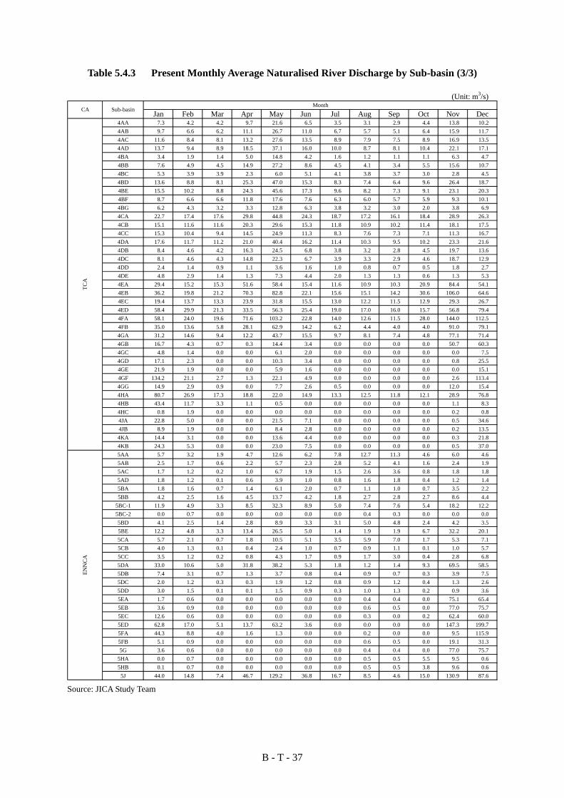
B - T - 37
Table 5.4.3 Present Monthly Average Naturalised River Discharge by Sub-basin (3/3)
(Unit: m3/s)
Jan Feb Mar Apr May Jun Jul Aug Sep Oct Nov Dec4AA 7.3 4.2 4.2 9.7 21.6 6.5 3.5 3.1 2.9 4.4 13.8 10.2
4AB 9.7 6.6 6.2 11.1 26.7 11.0 6.7 5.7 5.1 6.4 15.9 11.7
4AC 11.6 8.4 8.1 13.2 27.6 13.5 8.9 7.9 7.5 8.9 16.9 13.5
4AD 13.7 9.4 8.9 18.5 37.1 16.0 10.0 8.7 8.1 10.4 22.1 17.1
4BA 3.4 1.9 1.4 5.0 14.8 4.2 1.6 1.2 1.1 1.1 6.3 4.7
4BB 7.6 4.9 4.5 14.9 27.2 8.6 4.5 4.1 3.4 5.5 15.6 10.7
4BC 5.3 3.9 3.9 2.3 6.0 5.1 4.1 3.8 3.7 3.0 2.8 4.5
4BD 13.6 8.8 8.1 25.3 47.0 15.3 8.3 7.4 6.4 9.6 26.4 18.7
4BE 15.5 10.2 8.8 24.3 45.6 17.3 9.6 8.2 7.3 9.1 23.1 20.3
4BF 8.7 6.6 6.6 11.8 17.6 7.6 6.3 6.0 5.7 5.9 9.3 10.1
4BG 6.2 4.3 3.2 3.3 12.8 6.3 3.8 3.2 3.0 2.0 3.8 6.9
4CA 22.7 17.4 17.6 29.8 44.8 24.3 18.7 17.2 16.1 18.4 28.9 26.3
4CB 15.1 11.6 11.6 20.3 29.6 15.3 11.8 10.9 10.2 11.4 18.1 17.5
4CC 15.3 10.4 9.4 14.5 24.9 11.3 8.3 7.6 7.3 7.1 11.3 16.7
4DA 17.6 11.7 11.2 21.0 40.4 16.2 11.4 10.3 9.5 10.2 23.3 21.6
4DB 8.4 4.6 4.2 16.3 24.5 6.8 3.8 3.2 2.8 4.5 19.7 13.6
4DC 8.1 4.6 4.3 14.8 22.3 6.7 3.9 3.3 2.9 4.6 18.7 12.9
4DD 2.4 1.4 0.9 1.1 3.6 1.6 1.0 0.8 0.7 0.5 1.8 2.7
4DE 4.8 2.9 1.4 1.3 7.3 4.4 2.0 1.3 1.3 0.6 1.3 5.3
4EA 29.4 15.2 15.3 51.6 58.4 15.4 11.6 10.9 10.3 20.9 84.4 54.1
4EB 36.2 19.8 21.2 70.3 82.8 22.1 15.6 15.1 14.2 30.6 106.0 64.6
4EC 19.4 13.7 13.3 23.9 31.8 15.5 13.0 12.2 11.5 12.9 29.3 26.7
4ED 58.4 29.9 21.3 33.5 56.3 25.4 19.0 17.0 16.0 15.7 56.8 79.4
4FA 58.1 24.0 19.6 71.6 103.2 22.8 14.0 12.6 11.5 28.0 144.0 112.5
4FB 35.0 13.6 5.8 28.1 62.9 14.2 6.2 4.4 4.0 4.0 91.0 79.1
4GA 31.2 14.6 9.4 12.2 43.7 15.5 9.7 8.1 7.4 4.8 77.1 71.4
4GB 16.7 4.3 0.7 0.3 14.4 3.4 0.0 0.0 0.0 0.0 50.7 60.3
4GC 4.8 1.4 0.0 0.0 6.1 2.0 0.0 0.0 0.0 0.0 0.0 7.5
4GD 17.1 2.3 0.0 0.0 10.3 3.4 0.0 0.0 0.0 0.0 0.8 25.5
4GE 21.9 1.9 0.0 0.0 5.9 1.6 0.0 0.0 0.0 0.0 0.0 15.1
4GF 134.2 21.1 2.7 1.3 22.1 4.9 0.0 0.0 0.0 0.0 2.6 113.4
4GG 14.9 2.9 0.9 0.0 7.7 2.6 0.5 0.0 0.0 0.0 12.0 15.4
4HA 80.7 26.9 17.3 18.8 22.0 14.9 13.3 12.5 11.8 12.1 28.9 76.8
4HB 43.4 11.7 3.3 1.1 0.5 0.0 0.0 0.0 0.0 0.0 1.1 8.3
4HC 0.8 1.9 0.0 0.0 0.0 0.0 0.0 0.0 0.0 0.0 0.2 0.8
4JA 22.8 5.0 0.0 0.0 21.5 7.1 0.0 0.0 0.0 0.0 0.5 34.6
4JB 8.9 1.9 0.0 0.0 8.4 2.8 0.0 0.0 0.0 0.0 0.2 13.5
4KA 14.4 3.1 0.0 0.0 13.6 4.4 0.0 0.0 0.0 0.0 0.3 21.8
4KB 24.3 5.3 0.0 0.0 23.0 7.5 0.0 0.0 0.0 0.0 0.5 37.0
5AA 5.7 3.2 1.9 4.7 12.6 6.2 7.8 12.7 11.3 4.6 6.0 4.6
5AB 2.5 1.7 0.6 2.2 5.7 2.3 2.8 5.2 4.1 1.6 2.4 1.9
5AC 1.7 1.2 0.2 1.0 6.7 1.9 1.5 2.6 3.6 0.8 1.8 1.8
5AD 1.8 1.2 0.1 0.6 3.9 1.0 0.8 1.6 1.8 0.4 1.2 1.4
5BA 1.8 1.6 0.7 1.4 6.1 2.0 0.7 1.1 1.0 0.7 3.5 2.2
5BB 4.2 2.5 1.6 4.5 13.7 4.2 1.8 2.7 2.8 2.7 8.6 4.4
5BC-1 11.9 4.9 3.3 8.5 32.3 8.9 5.0 7.4 7.6 5.4 18.2 12.2
5BC-2 0.0 0.7 0.0 0.0 0.0 0.0 0.0 0.4 0.3 0.0 0.0 0.0
5BD 4.1 2.5 1.4 2.8 8.9 3.3 3.1 5.0 4.8 2.4 4.2 3.5
5BE 12.2 4.8 3.3 13.4 26.5 5.0 1.4 1.9 1.9 6.7 32.2 20.1
5CA 5.7 2.1 0.7 1.8 10.5 5.1 3.5 5.9 7.0 1.7 5.3 7.1
5CB 4.0 1.3 0.1 0.4 2.4 1.0 0.7 0.9 1.1 0.1 1.0 5.7
5CC 3.5 1.2 0.2 0.8 4.3 1.7 0.9 1.7 3.0 0.4 2.8 6.8
5DA 33.0 10.6 5.0 31.8 38.2 5.3 1.8 1.2 1.4 9.3 69.5 58.5
5DB 7.4 3.1 0.7 1.3 3.7 0.8 0.4 0.9 0.7 0.3 3.9 7.5
5DC 2.0 1.2 0.3 0.3 1.9 1.2 0.8 0.9 1.2 0.4 1.3 2.6
5DD 3.0 1.5 0.1 0.1 1.5 0.9 0.3 1.0 1.3 0.2 0.9 3.6
5EA 1.7 0.6 0.0 0.0 0.0 0.0 0.0 0.4 0.4 0.0 75.1 65.4
5EB 3.6 0.9 0.0 0.0 0.0 0.0 0.0 0.6 0.5 0.0 77.0 75.7
5EC 12.6 0.6 0.0 0.0 0.0 0.0 0.0 0.3 0.0 0.2 62.4 60.0
5ED 62.8 17.0 5.1 13.7 63.2 3.6 0.0 0.0 0.0 0.0 147.3 199.7
5FA 44.3 8.8 4.0 1.6 1.3 0.0 0.0 0.2 0.0 0.0 9.5 115.9
5FB 5.1 0.9 0.0 0.0 0.0 0.0 0.0 0.6 0.5 0.0 19.1 31.3
5G 3.6 0.6 0.0 0.0 0.0 0.0 0.0 0.4 0.4 0.0 77.0 75.7
5HA 0.0 0.7 0.0 0.0 0.0 0.0 0.0 0.5 0.5 5.5 9.5 0.6
5HB 0.1 0.7 0.0 0.0 0.0 0.0 0.0 0.5 0.5 3.8 9.6 0.6
5J 44.0 14.8 7.4 46.7 129.2 36.8 16.7 8.5 4.6 15.0 130.9 87.6
Sub-basinMonth
TC
AE
NN
CA
CA
Source: JICA Study Team

B - T - 38
Table 5.4.4 Future Monthly Average Naturalised River Discharge by Sub-basin (1/3)
(Unit: m3/s)
Jan Feb Mar Apr May Jun Jul Aug Sep Oct Nov Dec1AA 1.9 1.2 1.8 6.3 9.9 5.0 3.5 4.2 5.1 5.9 6.0 3.1
1AB 4.4 3.0 4.1 12.0 18.0 10.7 8.7 10.3 11.0 12.1 11.7 6.4
1AC 0.4 0.1 0.3 2.1 3.7 2.1 1.3 1.6 2.0 2.2 2.3 0.9
1AD 2.4 1.5 2.0 7.6 12.8 6.6 4.1 3.9 5.5 6.9 7.8 4.7
1AE 1.2 0.8 1.0 3.2 5.4 2.7 1.5 1.3 1.9 2.7 3.3 2.3
1AF 3.2 2.2 2.9 8.3 13.1 7.2 4.8 4.8 6.2 7.5 8.4 5.3
1AG 2.1 1.2 1.7 6.3 10.6 5.5 3.4 3.3 4.4 5.4 6.4 3.9
1AH 1.5 0.8 1.3 6.4 10.7 4.3 2.0 2.0 3.4 5.2 6.4 3.6
1BA 2.8 1.6 1.7 7.0 11.0 6.6 7.9 9.3 5.0 6.2 7.1 3.9
1BB 9.8 6.6 7.0 22.3 36.5 22.9 27.6 31.5 19.0 22.4 23.0 12.8
1BC 5.1 3.5 3.4 8.6 17.8 14.0 15.5 18.1 14.6 15.0 13.0 7.2
1BD 6.9 5.4 5.9 8.7 14.1 11.2 11.2 14.7 12.7 11.7 11.1 8.2
1BE 7.9 4.9 4.9 13.6 30.6 24.2 24.0 31.0 26.9 26.6 23.6 12.8
1BG 9.9 7.2 8.2 19.4 32.6 24.1 23.1 30.6 27.5 27.2 23.7 13.2
1BH 6.7 4.8 5.8 14.8 23.8 17.1 15.4 19.8 19.0 18.9 17.0 9.3
1CA 6.8 5.2 5.6 9.1 13.0 9.8 11.1 13.4 9.9 9.4 9.7 7.7
1CB 6.5 4.6 4.9 10.7 14.7 10.8 12.9 15.6 11.2 10.4 10.3 7.7
1CC 10.9 8.7 9.6 16.9 20.9 16.4 19.4 21.7 16.7 16.4 15.6 12.7
1CD 19.5 14.7 16.5 31.9 44.3 33.5 38.3 46.6 35.3 32.8 31.4 22.9
1CE 4.8 3.9 4.6 8.1 11.4 9.2 9.4 12.1 10.5 9.8 8.4 5.8
1DA 9.1 7.3 9.4 18.7 25.4 18.9 17.5 22.5 21.8 21.0 18.9 12.3
1DB 14.6 11.6 14.1 28.1 39.5 27.9 25.2 29.5 29.1 30.3 28.4 18.3
1DC 6.6 5.0 5.9 11.0 17.0 12.4 10.1 11.2 12.4 12.4 12.5 8.9
1DD 7.2 5.6 6.6 12.1 18.5 12.8 9.9 10.2 11.6 12.2 13.1 9.8
1EA 14.9 12.4 15.4 27.1 32.6 25.8 24.9 29.4 27.0 26.4 24.2 18.2
1EB 12.2 10.2 12.2 19.9 24.1 18.4 16.9 18.9 18.7 19.1 18.1 14.6
1EC 7.3 6.2 7.2 11.5 14.3 11.2 10.5 12.4 12.6 12.8 12.0 9.1
1ED 2.9 2.3 2.7 4.9 6.9 4.6 3.8 4.0 4.4 4.7 4.9 3.8
1EE 3.2 1.7 2.1 6.7 15.2 8.0 3.4 3.4 5.5 6.9 9.2 6.8
1EF 1.8 0.2 0.8 6.5 17.3 6.2 0.4 0.9 3.1 5.4 9.4 6.6
1EG 5.9 3.1 4.2 12.8 21.4 12.1 7.2 7.4 8.8 11.2 13.2 10.7
1FA 1.8 1.2 1.3 4.6 6.0 4.5 5.5 6.5 4.6 4.3 4.2 2.7
1FB 8.1 6.3 8.0 17.0 21.7 17.1 18.5 21.0 17.4 16.5 15.8 10.8
1FC 4.9 3.8 4.8 9.2 12.1 9.6 9.6 10.9 9.9 9.2 8.8 6.7
1FD 7.8 5.9 7.5 16.5 21.3 16.3 17.2 18.9 16.0 15.6 15.6 11.0
1FE 12.3 8.9 12.1 28.4 36.6 26.1 22.1 25.0 24.4 24.5 24.1 18.6
1FF 1.9 0.6 1.5 7.2 9.6 5.6 3.3 3.3 3.5 4.3 4.9 4.1
1FG 4.5 0.6 3.0 17.5 28.5 8.2 0.7 1.8 4.2 8.8 15.4 12.8
1GA 6.6 4.7 6.5 20.7 24.0 15.7 17.8 20.9 15.2 14.7 15.1 10.1
1GB 6.3 3.5 6.5 24.3 25.2 14.6 12.8 14.8 13.4 14.7 15.8 10.5
1GC 14.1 11.3 13.8 31.8 39.2 25.5 27.7 35.7 28.0 25.8 25.3 19.6
1GD 3.7 1.3 2.9 18.4 16.7 7.0 2.6 4.6 4.3 6.5 8.0 6.3
1GE 3.6 1.7 2.8 14.8 13.6 6.1 2.2 3.7 3.3 6.2 7.7 5.8
1GF 2.6 0.8 2.2 12.8 11.5 4.2 0.7 1.3 0.7 3.5 5.6 5.6
1GG 5.2 3.8 6.0 18.0 19.7 11.6 11.9 14.7 11.4 11.1 11.6 7.8
1HA1 5.1 2.9 5.7 15.2 15.9 9.1 6.1 6.5 6.0 7.5 9.5 9.2
1HA2 1.6 0.3 0.9 7.2 3.2 1.2 0.2 0.3 0.2 0.9 2.1 4.5
1HB1 3.1 0.7 1.6 7.3 10.8 5.4 2.2 1.4 1.5 3.1 5.1 6.8
1HB2 2.4 0.8 2.1 7.3 8.2 4.5 2.1 1.6 1.4 2.4 3.7 4.6
1HC 3.2 0.6 1.3 4.7 8.7 4.9 1.3 0.3 0.2 1.3 2.9 6.4
1HD 0.0 0.0 0.0 0.0 0.0 0.0 0.0 0.0 0.0 0.0 0.0 0.0
1HE 8.5 4.4 8.0 24.6 30.1 18.5 9.6 6.4 7.5 11.7 16.1 17.2
1HF 6.1 2.7 5.8 18.9 26.6 13.4 6.2 3.0 4.5 9.1 14.4 14.0
1HG 5.8 1.5 2.8 12.5 20.4 11.2 2.6 0.2 0.2 1.1 3.3 8.2
1JA 2.8 0.7 1.9 9.0 13.8 3.7 0.8 0.2 0.3 1.4 4.7 6.1
1JB 18.3 15.2 19.9 39.7 42.7 29.3 26.8 29.3 27.6 27.3 29.8 25.2
1JC 3.9 3.2 4.7 10.2 10.8 7.0 5.9 5.9 5.9 6.4 7.2 5.6
1JD 8.9 7.4 9.9 18.8 20.8 14.1 13.2 14.1 13.4 13.8 14.4 11.4
1JE 7.3 6.1 7.9 14.0 15.2 11.3 9.5 9.2 9.3 10.4 11.2 9.8
1JF 8.9 7.6 11.6 22.8 20.4 12.9 9.3 7.9 9.6 11.3 15.2 14.4
1JG1 23.7 18.6 26.5 52.9 54.6 38.4 30.2 27.9 29.5 32.0 38.4 35.7
1JG2 4.2 2.6 4.0 11.6 14.3 9.0 5.6 4.6 5.3 6.6 8.1 7.8
1KA 1.5 0.8 1.1 3.5 4.7 2.5 1.2 0.8 1.1 1.5 2.1 3.0
1KB 5.5 3.5 6.1 15.8 20.1 10.2 5.0 3.5 4.9 7.9 11.0 10.4
1KC 39.3 24.5 41.1 103.8 131.0 58.8 28.6 19.2 24.4 38.6 58.4 67.7
1LA1 40.1 31.3 47.0 98.5 102.0 48.2 24.1 14.2 16.4 29.1 45.4 61.3
1LA2 16.2 13.1 17.4 42.8 40.0 25.0 19.7 19.5 19.6 20.2 26.4 26.6
1LA3 17.7 15.4 18.3 37.2 38.6 21.3 12.3 8.0 9.6 11.9 15.1 24.3
1LB1 30.7 29.4 32.9 79.4 72.5 29.3 13.2 6.3 6.6 8.9 15.5 35.1
1LB2 26.9 21.9 27.6 67.1 62.0 36.0 24.0 21.2 21.9 23.3 33.0 42.9
LV
NC
AL
VS
CA
CA Sub-basinMonth

B - T - 39
Table 5.4.4 Future Monthly Average Naturalised River Discharge by Sub-basin (2/3)
(Unit: m3/s)
Jan Feb Mar Apr May Jun Jul Aug Sep Oct Nov Dec2AA 21.2 21.2 25.5 66.5 62.4 24.2 8.0 1.7 2.8 5.5 8.5 25.5
2AB 0.1 0.1 0.1 0.1 0.1 0.1 0.1 0.1 0.1 0.1 0.1 0.1
2BA 0.0 0.0 0.0 0.0 0.0 0.0 0.0 0.0 0.0 0.0 0.1 0.0
2BB 8.5 3.5 2.0 13.0 35.6 29.0 39.0 46.7 28.1 31.6 26.7 10.9
2BC 13.7 5.6 3.2 20.9 57.2 46.6 62.8 75.0 45.2 50.8 43.0 17.5
2BD 11.2 4.0 2.7 20.3 50.8 39.4 44.5 58.9 41.9 46.5 40.1 17.2
2CA 0.0 0.0 0.0 0.0 0.1 0.1 0.0 0.0 0.2 0.5 0.4 0.8
2CB 0.0 0.0 0.0 0.0 0.0 0.0 0.0 0.0 0.0 0.0 0.0 0.0
2CC 27.7 13.7 8.3 63.5 92.6 56.0 72.7 89.9 41.6 39.8 52.1 35.4
2D 24.9 9.0 4.9 35.0 97.6 63.8 73.0 105.4 52.3 58.1 65.2 34.0
2EA 7.3 1.1 0.7 18.6 17.3 8.6 4.9 21.7 7.7 8.9 15.8 14.3
2EB 2.2 1.0 0.6 2.9 4.7 3.2 4.5 6.5 4.0 2.8 3.3 3.0
2EC 3.7 1.6 1.0 4.7 7.9 5.2 7.5 10.8 6.6 4.6 5.4 5.0
2ED 3.4 2.1 1.5 3.3 8.3 5.4 5.5 9.2 7.7 5.8 5.5 6.4
2EE 3.1 2.0 1.5 3.6 8.4 6.4 8.7 14.0 11.1 7.1 6.3 5.9
2EF 6.0 2.9 1.9 12.7 18.9 12.6 18.6 26.0 13.3 9.3 10.9 8.4
2EG1 2.8 1.9 1.4 3.3 7.7 5.9 8.0 12.9 10.2 6.6 5.8 5.5
2EG2 2.0 1.1 0.7 2.9 5.1 3.3 4.1 7.0 4.5 3.2 3.4 3.3
2EH 6.6 3.7 2.5 9.6 17.0 10.9 13.7 23.4 15.0 10.8 11.5 11.1
2EJ 3.1 1.1 1.0 8.7 9.3 5.6 7.3 10.7 3.9 3.2 5.2 3.6
2EK 1.5 0.4 0.3 3.3 2.0 0.9 0.9 4.4 1.6 1.8 3.2 3.3
2FA 2.6 1.0 0.6 4.5 5.6 3.5 5.5 8.4 3.1 2.3 3.9 3.4
2FB 1.6 0.9 0.7 1.4 3.2 2.1 2.1 2.6 2.6 2.2 2.7 2.7
2FC 0.4 0.2 0.2 0.3 0.8 0.5 0.5 0.7 0.7 0.6 0.7 0.7
2GA 4.5 3.0 2.1 4.9 8.9 5.9 5.4 7.1 6.5 5.4 6.5 6.4
2GB 2.9 1.8 1.3 3.1 5.0 3.3 2.8 2.5 2.3 2.1 3.4 3.1
2GC 9.5 5.0 3.7 11.6 17.9 11.4 10.6 9.6 9.3 9.1 14.4 11.5
2GD 10.4 5.4 5.1 18.3 27.6 15.0 9.0 6.0 6.9 10.1 19.1 15.0
2H-1 14.7 7.6 7.2 25.8 38.9 21.1 12.7 8.5 9.7 14.2 27.0 21.1
2H-2 6.0 6.4 3.0 7.7 12.3 4.6 1.1 0.3 0.1 0.0 0.8 5.2
2H-3 7.8 8.7 3.6 11.7 17.5 4.3 1.1 0.3 0.1 0.0 1.1 6.6
2J 3.1 3.0 1.2 3.5 5.1 1.4 0.2 0.0 0.0 0.0 0.1 2.5
2KA 0.0 0.0 0.0 0.0 0.0 0.0 0.0 0.0 0.0 0.0 0.0 0.0
2KB 33.4 27.9 25.6 73.5 79.5 36.9 17.3 9.1 8.5 9.2 22.3 40.2
2KC 8.5 6.7 5.0 13.3 17.0 5.5 3.3 2.9 2.6 2.4 4.7 10.0
3AA 6.2 6.2 2.2 5.2 12.3 3.1 0.8 0.2 0.0 0.0 0.0 6.8
3AB 10.3 8.7 6.6 14.3 19.9 7.7 4.1 3.5 3.3 3.6 6.8 11.5
3AC 7.3 6.0 3.0 7.8 10.0 3.0 0.6 0.3 0.2 0.2 1.9 5.7
3BA 5.5 3.4 1.9 7.3 10.3 2.7 0.5 0.2 0.1 0.1 3.2 7.6
3BB 3.9 2.9 2.4 6.3 9.3 2.9 1.2 0.8 0.7 1.0 3.5 5.6
3BC 3.4 2.7 2.5 6.4 8.2 2.7 1.3 1.0 0.9 1.3 3.6 4.9
3BD 12.7 9.6 9.3 19.4 27.2 11.8 7.6 6.3 5.7 6.4 12.8 16.5
3CB 5.2 4.0 3.7 8.9 11.7 4.6 2.7 2.2 2.0 2.2 5.4 7.1
3DA 9.7 7.8 7.6 13.1 16.7 8.7 6.8 6.1 5.7 6.1 9.5 11.6
3DB 8.4 4.7 3.8 12.0 10.6 2.7 3.6 4.1 4.0 3.8 9.2 13.8
3EA 8.3 2.4 1.0 8.4 7.7 1.7 0.3 0.0 0.0 0.0 7.8 16.3
3EB 10.7 4.5 2.1 12.9 9.3 1.5 0.2 0.0 0.0 0.0 8.3 16.2
3EC 10.8 3.9 2.2 14.0 9.3 1.1 0.0 0.0 0.0 0.0 9.4 18.8
3ED 10.2 3.4 2.2 13.8 9.3 1.1 0.0 0.0 0.0 0.0 8.7 18.4
3FA 4.6 1.2 0.5 4.5 3.6 0.5 0.0 0.0 0.0 0.0 2.5 8.5
3FB 38.3 12.2 4.6 19.4 16.4 5.7 3.2 3.0 2.8 2.6 9.0 39.6
3G 24.8 8.3 1.0 6.4 6.4 2.2 0.1 0.0 0.0 0.0 0.9 36.1
3HA 14.3 8.5 2.4 16.2 5.1 1.1 0.1 0.0 0.0 0.0 0.3 7.8
3HB 1.7 1.3 0.1 0.4 0.7 0.1 0.0 0.0 0.0 0.0 0.0 2.8
3HC 2.5 2.5 0.0 0.0 1.4 0.4 0.0 0.0 0.0 0.0 0.2 5.0
3HD1 1.1 0.1 0.0 0.0 1.0 1.1 0.1 0.0 0.0 0.0 1.7 2.6
3HD2 0.5 0.6 0.0 0.0 2.2 1.9 0.4 0.0 0.0 0.0 3.5 2.6
3J 0.0 0.0 0.0 0.0 0.0 0.0 0.0 0.0 0.0 0.0 0.0 0.0
3K 2.7 2.2 0.0 1.1 0.3 0.0 0.0 0.0 0.0 0.0 0.2 0.4
3LA 4.8 2.9 1.5 3.9 22.5 3.6 1.7 0.4 0.2 4.0 16.2 3.9
3LB 2.1 0.6 0.0 0.1 4.0 0.4 0.1 0.0 0.0 5.0 11.8 1.2
3MA-1 0.0 0.0 0.0 0.0 0.0 0.0 0.0 0.0 0.0 0.0 0.0 0.0
3MA-2 2.4 1.2 0.1 0.8 0.5 0.1 0.1 0.1 0.1 0.1 1.8 2.2
3MB 0.9 0.4 0.0 0.0 1.9 0.2 0.1 0.0 0.0 0.3 3.1 0.3
3MC 0.9 0.1 0.0 0.0 5.8 0.4 0.3 0.1 0.0 3.4 6.1 0.4
3MD1 0.0 0.0 0.0 0.0 2.2 0.3 0.1 0.0 0.0 1.5 2.0 0.0
3MD2 1.7 0.1 0.0 0.2 22.4 3.0 1.0 0.1 0.0 6.8 6.6 0.6
3N 0.1 0.0 0.0 0.0 1.4 0.2 0.1 0.0 0.0 0.6 0.6 0.1
RV
CA
AC
A
CA Sub-basinMonth

B - T - 40
Table 5.4.4 Future Monthly Average Naturalised River Discharge by Sub-basin (3/3)
(Unit: m3/s)
Jan Feb Mar Apr May Jun Jul Aug Sep Oct Nov Dec4AA 0.0 0.7 0.2 0.9 0.6 0.1 0.0 0.0 0.0 0.0 0.0 0.4
4AB 8.5 4.9 5.2 14.4 26.3 6.9 3.8 3.3 3.0 5.1 12.6 13.8
4AC 10.5 6.4 6.4 16.2 29.7 10.0 5.5 4.2 3.6 6.2 14.0 13.9
4AD 6.2 2.8 2.6 12.1 23.6 6.7 2.2 0.8 0.7 3.0 10.1 9.4
4BA 10.1 5.3 5.6 20.8 35.3 10.8 5.1 3.2 2.9 7.1 17.9 16.4
4BB 4.9 2.7 2.8 9.5 17.6 4.7 2.3 1.8 1.6 2.3 7.1 7.4
4BC 11.3 8.0 9.0 23.2 32.0 11.3 7.5 6.5 6.0 10.2 19.8 17.3
4BD 0.0 0.0 0.0 0.5 1.1 0.0 0.0 0.0 0.0 0.0 0.3 0.1
4BE 18.1 12.5 13.8 37.9 53.4 18.0 11.5 9.8 9.0 15.7 31.8 28.2
4BF 15.1 9.0 9.1 32.6 46.5 15.1 7.8 5.8 5.0 9.4 24.7 24.0
4BG 3.4 1.5 1.3 10.3 11.6 1.4 0.0 0.0 0.0 0.2 4.7 5.5
4CA 4.8 1.5 0.8 6.0 11.3 2.3 0.1 0.0 0.0 0.0 2.7 6.2
4CB 10.5 6.6 6.8 24.9 33.9 11.9 6.0 3.7 3.2 7.6 19.5 17.8
4CC 5.6 3.3 3.1 15.8 21.2 5.6 1.6 0.5 0.3 2.6 10.4 10.3
4DA 0.0 0.0 0.0 0.0 0.0 0.0 0.0 0.0 0.0 0.0 0.0 0.0
4DB 2.6 0.3 0.4 4.8 9.8 0.0 0.0 0.0 0.0 0.0 1.3 2.4
4DC 22.0 12.8 13.6 47.8 58.7 15.8 10.7 9.8 9.3 13.6 39.2 35.3
4DD 9.4 5.5 5.7 21.1 25.4 7.0 4.3 3.8 3.6 6.6 19.8 16.3
4DE 3.5 1.6 0.5 3.3 5.7 1.3 0.4 0.3 0.2 0.1 1.9 4.7
4EA 6.7 2.3 0.6 4.2 10.2 3.0 0.3 0.0 0.0 0.0 1.7 7.8
4EB 42.6 22.0 21.2 64.8 69.8 22.9 16.5 15.1 14.3 25.3 83.7 75.9
4EC 45.4 22.2 22.7 88.8 96.2 21.3 14.3 13.5 12.7 30.2 98.7 79.3
4ED 9.7 3.3 1.3 21.3 24.2 2.1 0.0 0.0 0.0 1.9 19.6 20.2
4FA 66.9 22.7 6.5 59.5 65.8 4.9 0.0 0.0 0.0 0.0 51.2 116.9
4FB 85.7 41.0 36.2 104.2 131.5 36.1 27.7 26.1 24.7 40.6 155.6 162.9
4GA 33.2 9.2 3.0 35.6 60.9 9.7 1.7 0.2 0.0 3.9 82.4 92.2
4GB 42.9 16.2 11.2 19.5 45.7 15.2 10.6 9.7 9.1 7.2 76.4 91.5
4GC 31.7 6.3 1.3 1.9 18.3 6.0 1.2 0.4 0.2 0.0 47.4 68.8
4GD 9.9 2.8 0.4 0.0 10.3 4.6 0.7 0.1 0.0 0.0 0.1 10.6
4GE 30.6 6.7 1.3 0.4 19.8 9.2 1.9 0.7 0.3 0.1 0.7 32.4
4GF 31.6 4.3 0.7 0.0 11.0 6.0 1.1 0.2 0.0 0.0 0.1 21.3
4GG 152.5 28.2 5.2 12.1 32.4 18.1 4.2 1.3 0.5 0.3 7.3 137.4
4HA 33.9 11.1 2.8 0.1 23.1 27.3 5.4 0.6 0.0 0.0 2.2 32.2
4HB 69.9 16.6 6.7 21.5 18.0 5.4 2.8 1.5 1.0 1.1 24.3 76.3
4HC 59.2 16.1 4.6 2.1 1.8 0.8 0.4 0.3 0.3 0.2 0.7 18.3
4JA 4.0 3.4 0.2 0.0 0.0 0.0 0.0 0.0 0.0 0.0 0.1 1.5
4JB 0.0 0.0 0.0 0.0 0.0 0.0 0.0 0.0 0.0 0.0 0.0 0.0
4KA 0.0 0.0 0.0 0.0 0.0 0.0 0.0 0.0 0.0 0.0 0.0 0.0
4KB 0.0 0.0 0.0 0.0 0.0 0.0 0.0 0.0 0.0 0.0 0.0 0.0
5AA 5.2 2.5 2.0 8.7 11.6 6.1 8.1 10.7 7.2 5.4 7.4 6.9
5AB 2.0 0.8 0.6 3.9 4.7 2.1 2.9 3.4 2.2 2.0 3.2 2.6
5AC 2.9 0.7 0.2 3.5 5.9 1.8 1.6 2.1 1.0 0.7 2.8 3.2
5AD 1.7 0.5 0.2 1.6 3.1 0.8 0.8 1.1 0.7 0.5 1.6 2.1
5BA 2.1 1.0 0.8 2.8 7.3 2.0 0.7 0.5 0.4 0.9 3.1 3.1
5BB 4.3 1.9 1.7 7.8 14.4 4.1 1.8 1.4 1.3 3.2 7.9 6.7
5BC-1 11.2 4.4 3.3 15.4 31.1 8.5 5.1 5.0 4.1 6.0 17.4 17.3
5BC-2 0.0 0.0 0.0 0.0 0.0 0.0 0.0 0.0 0.0 0.0 0.0 0.0
5BD 3.7 1.8 1.5 4.9 7.3 3.1 3.2 3.6 2.8 2.7 4.7 4.7
5BE 12.2 3.8 4.3 19.7 26.9 5.8 1.4 0.9 0.7 6.6 30.3 26.3
5CA 4.8 2.0 1.9 13.1 11.0 5.3 3.7 5.8 2.9 1.7 6.2 7.9
5CB 2.3 0.5 0.1 9.2 3.8 1.0 0.5 0.4 0.3 0.1 1.4 4.6
5CC 2.6 0.6 0.3 11.8 7.3 1.8 0.6 0.5 0.5 0.2 3.0 6.4
5DA 30.0 9.3 7.9 40.6 34.8 4.8 1.6 0.9 0.6 10.9 67.6 68.7
5DB 7.0 2.2 0.8 3.6 3.5 0.8 0.3 0.1 0.0 0.1 4.3 8.7
5DC 2.4 0.7 0.3 1.7 2.7 1.4 0.9 0.7 0.6 0.4 1.5 3.4
5DD 2.7 0.7 0.3 3.2 2.3 0.9 0.4 0.5 0.5 0.2 0.9 3.9
5EA 27.9 0.2 0.0 0.2 0.1 0.0 0.0 0.0 0.0 0.8 92.4 67.2
5EB 33.1 0.7 0.0 6.6 15.5 0.9 0.0 0.0 0.0 3.1 149.6 98.5
5EC 33.1 0.7 0.5 12.6 38.7 5.3 3.1 2.1 1.4 2.7 101.6 80.0
5ED 67.0 17.8 5.6 16.7 52.8 2.8 0.0 0.0 0.0 0.0 151.8 211.6
5FA 48.4 10.4 4.6 1.6 0.0 0.0 0.0 0.0 0.0 0.0 5.0 103.1
5FB 10.5 0.0 0.0 0.0 0.0 0.0 0.0 0.0 0.0 0.0 17.5 26.7
5G 33.1 0.7 0.0 6.6 15.5 0.9 0.0 0.0 0.0 3.1 149.6 98.5
5HA 0.0 0.0 0.0 0.0 0.0 0.0 0.0 0.0 0.0 6.1 5.7 1.0
5HB 0.0 0.0 0.0 0.0 0.0 0.0 0.0 0.0 0.0 5.3 7.2 0.7
5J 44.0 13.9 7.4 46.7 129.2 36.8 16.7 7.9 4.0 15.0 130.9 87.6
Sub-basinMonth
TC
AE
NN
CA
CA
Source: JICA Study Team

B - T - 41
Table 6.2.1 Selection of Stations for Frequency Analysis Based on Data Availability (1/2) Numbers of valid years of which data availability is more than the criteria.
Annual Data
Available
1AD02 1AH01 1BD02 1BG07 1CE01 1EE01 1EF01 1EG02 1FC01 1FE01
Malakisi Sio Large Zoia
Rongai Kipkaren Nzoia at Ruambwa
Wuoroya Kimondi Yala
10% 17 26 20 27 15 13 26 20 19 19 20% 16 26 20 27 13 10 26 20 19 18 30% 15 26 20 26 12 10 26 20 18 18 40% 14 25 19 23 11 10 26 20 18 18 50% 14 24 19 23 10 9 26 17 18 18 60% 13 22 17 22 9 7 25 16 17 17 70% 11 21 16 22 8 6 24 13 14 14 80% 8 20 12 19 7 6 21 9 14 14 90% 4 20 12 12 4 5 19 3 14 12 100% 2 7 6 5 2 2 17 2 9 12
Annual
Data Available
1FG01 1FG02 1GB05 1GC04 1GD03 1GD07 1GG01 1JG01 1KB05 1KC03
Yala Yala Ainamatua Tugenon Nyando Nyando Namuting Sondu Gucha Migori
Migori
10% 22 18 24 29 22 15 26 12 21 21 20% 21 17 22 29 22 15 25 12 21 21 30% 21 17 21 27 21 14 25 12 17 21 40% 21 17 21 27 20 14 24 12 17 20 50% 20 17 21 27 20 14 24 11 17 19 60% 19 14 20 26 18 14 23 10 17 18 70% 18 14 18 25 14 14 22 10 15 18 80% 11 13 15 23 11 14 21 9 15* 17* 90% 8 10 10 22 8 9 20 7 10 16 100% 3 4 2 15 3 2 15 6 8 13
Annual
Data Available
1LA03 2B07 2B33 2C07 2C16 2EE07 2K06 3BA32 3BC08 3DA02
Nyangores Suam Suam Ndo Kerio Perkerra Seyabei Nairobi Ruiru Athi Munyu
10% 27 13 16 12 10 9 19 8 14 23 20% 27 12 15 10 10 9 18 8 14 22 30% 27 12 15 10 10 9 18 8 14 21 40% 26 10 15 7 10 9 18 6 14 20 50% 25 10 15 5 8 9 18 5 14 19 60% 24 10 14 5 8 9 16 5 14 17 70% 24 7 14 3 7 9 13 4 12 17 80% 22 6 13 2 6 7 13 3 12 16 90% 17 3 9 0 6 5 9 3 8 13 100% 4 1 7 0 3 2 5 0 3 2
Annual
Data Available
3HA12 4BC02 4BE01 4BE03 4CA02 4CB04 4DA10 4DC03 4EA07 4F13 Sabaki
Cableway Tana
Sagana Maragua Irati Chania Thika Thiba Rupingazi Mutonga
Grand Falls
10% 8 24 30 18 24 30 25 21 23 23 20% 7 24 29 17 24 30 24 21 23 23 30% 7 24 29 17 24 30 22 20 23 23 40% 6 24 27 17 24 28 22 20 23 21 50% 5 22 27 17 22 28 22 19 21 21 60% 3 21 27 15 21 28 22 19 18 21 70% 2 20 25 15 19 28 19 16 18 21 80% 1 18 24 13 14 21 18 16 18 16 90% 0 13 22 11 8 15 11 13 12 11 100% 0 1 11 10 0 1 2 0 9 1
Note1: The stations which has more than 15 years valid were selected for the subject of the frequency analysis. The valid year was defined which has more than 80% of data availability. The cells of selected stations are filled with light blue.
Note2: 1KB05 Gucha Migori and 1KC03 Migori are satisfied the standard selection mentioned in Note1. However, those are excluded for the seletion for the frequency analysis because there are strange discharge data of spike-like and difficult to find appropriate annual maximum discharge.
Source: JICA Study Team with original observed data by WRMA and MWI

B - T - 42
Table 6.2.1 Selection of Stations for Frequency Analysis Based on Data Availability (2/2) Numbers of valid years of which data availability is more than the criteria.
Annual Data
Available
4G01 4G02 5AC10 5AC15 5BB02 5BC04 5E03
Garissa Garsen Ewaso Narok
Ewaso Narok
Ewaso Ng’iro
Ewaso Ng’iro
Ewaso Ng’iro at
Archers' Post 10% 30 16 29 28 29 28 24 20% 30 15 29 28 29 27 24 30% 30 14 29 28 29 21 23 40% 30 13 29 28 28 19 21 50% 29 11 25 26 27 18 21 60% 27 10 15 22 27 17 21 70% 26 8 15 15 27 12 20 80% 24 7 14 8 27 8 19 90% 23 4 10 7 25 6 13
100% 6 3 6 4 3 1 10 Note1: The stations which has more than 15 years valid were selected for the subject of the frequency
analysis. The valid year was defined which has more than 80% of data availability. The cells of selected stations are filled with light blue.
Note2: 1KB05 Gucha Migori and 1KC03 Migori are satisfied the standard selection mentioned in Note1. However, those are excluded for the seletion for the frequency analysis because there are strange discharge data of spike-like and difficult to find appropriate annual maximum discharge.
Source: JICA Study Team with original observed data by WRMA and MWI
Table 6.2.2 Annual Maximum Flood Discharge Record (1/2) (m3/s)
1AH01 1BG07 1EF01 1GB05 1GC04 1GG01 1LA03 3DA02 4BC02
Year Sio Rongai Nzoia at Ruambwa Ainamatua Tugenon Namuting Nyangores Athi
Munyu Tana
Sagana 1980 46.71 6.88 292.94 10.63 4.47 9.61 19.62 217.59 106.86 1981 58.65 31.66 687.05 - 3.69 16.91 28.84 639.71 178.3 1982 60.75 25.91 774.91 - 3.1 18.96 28.35 - 303.89 1983 59.79 - 753.54 - 3.06 15.26 - 116.54 140.69 1984 51.64 8.94 - - 0.42 5.18 - 116.24 63.02 1985 65.09 9.15 - 19.86 3.1 21.98 - 186.08 198.46 1986 - - 288.82 14.75 3.85 9.12 11.7 548.59 194.18 1987 58.75 17.34 375.85 4.88 2.9 13.36 28.84 118.56 77.99 1988 62.41 31.66 920.45 21.14 3.2 24.14 28.76 721.79 359.73 1989 68.17 12.55 - 10.73 1.78 24.14 28.19 316.95 80.97 1990 65.06 11.73 538.40 10.63 5.62 24.13 28.76 316.77 112.35 1991 66.77 - 553.21 6.37 2.84 24.14 22.93 48.16 168.21 1992 46.04 17.04 774.10 21.15 4.68 24.14 28.43 175.98 49.33 1993 - 16.72 478.68 6.51 0.85 15.96 - 168.15 65.65 1994 63.79 - 611.66 13.34 - 24.14 - - 211.2 1995 66.55 23.58 619.31 - - 13.49 - 71.06 - 1996 65.06 - 389.90 - - 21.93 28.35 - - 1997 67.44 - 726.51 10.54 - - 28.84 - - 1998 - - 693.59 12.76 - 19.85 28.84 - - 1999 68.71 17.34 492.18 - - - - - - 2000 - 21.11 415.52 - 0.71 10.93 11.7 - - 2001 60.32 28.95 854.54 - 2.57 19.84 28.84 - 173.79 2002 68.82 6.31 862.72 - 1.05 12.5 28.76 - 238.44 2003 - 35.19 - - 2.38 - 27.81 730.69 151.9 2004 - - - - 0.96 - - 382.56 - 2005 - - - - 1.05 - 25 - - 2006 71.98 20.36 976.48 11.96 3.45 - 28.15 - - 2007 - - - 21.62 1.96 - 28.14 - - 2008 - - - - - - 18.96 - - 2009 - - - - 0.5 - - - - 2010 - - - - - - - - -
Source: JICA Study Team with original observed data from WRMA and MWI

B - T - 43
Table 6.2.2 Annual Maximum Flood Discharge Record (2/2) (m3/s)
4BE01 4CB04 4DA10 4DC03 4EA07 4F13 4G01 5BB02 5E03
Year Maragua Thika Thiba Rupingazi Mutonga Grand Falls Garissa Ewaso Ngiro
Ewaso Ng’iro at Archers' Post
1980 41.61 - 20.18 11.65 50.15 712.22 - 6.54 80.471981 158.88 64.95 44.89 21.13 76.57 809.95 596.17 11.03 371.841982 88.18 40.52 62.83 23.71 75.4 742.87 790.22 8.25 548.941983 82.44 24.86 56.74 17.21 69.29 592.95 487.59 4.88 86.811984 50.42 19.15 19.93 9.99 40.8 - 988.43 3.44 192.761985 103.87 44.04 38.63 23.65 57.52 621.79 656.97 4.45 169.671986 89.55 49.35 70.06 32.42 68.8 - 650.21 14.89 389.051987 31.08 15.77 41.56 17.9 40.89 - 203.83 8.6 169.021988 - 47.48 23.36 26.26 76.09 - 909.99 12.76 407.731989 86.01 49.77 26.97 16.68 91.51 - 832.26 7.39 480.41990 132.48 50.09 30.69 15.05 74.02 884.48 774.31 14.95 -1991 - 36.01 117.29 24.77 - 346.03 401.09 3.48 501992 120.91 - 30 11.44 65.42 453.31 456.95 15 213.711993 34.88 15.64 52.41 22.88 64.7 250.39 388.1 11.83 291.61994 - 52.16 - 30.13 91.12 486.11 849.07 11.96 -1995 - 41.21 87.34 - 82.82 - 540.19 3.06 185.871996 27.98 17.36 - - - 274.52 - 14.36 -1997 205.75 60.4 - - 92.7 - - 15.38 -1998 183.41 63.93 - - 91.65 - 1,024.10 13.87 -1999 - - 17.65 - - - 613.76 2.78 -2000 17.93 - - - - - 340.07 2.64 227.122001 - - - - - - - 9.49 95.132002 - 61.27 47.47 - - - 882.54 8.7 340.072003 479.22 - - - - - - 15.75 -2004 110.8 26.13 35.35 - - - 636.68 13.72 -2005 71.79 - - - - 219.86 - - -2006 - 33.25 - 13.64 - 328.17 1,395.83 10.61 -2007 84.7 - - - - 237.13 729.63 2.34 -2008 60.79 18.82 - - - - 633.78 - 352.792009 64.44 - - - - 311.46 511.78 - 133.552010 - - - - - - - - -
Source: JICA Study Team with original observed data from WRMA and MWI

B - T - 44
Table 6.2.3 Probable Flood Discharge based on Observed Record
Station Code Station Name
Evaluation of Fittness by SLSC
Validity *Probable Flood Discharge
LP3 Gumbel GEV LN3SQRT
- ET
Best PDF
10 year RP
25 year RP
50 year RP
100 year RP
1AH01 Sio 0.14 0.10 0.04 0.08 0.10 GEV invalid 70 71 71 71 1BG07 Rongai 0.06 0.04 0.03 0.04 0.05 GEV valid 32 37 41 44
1EF01 Nzoia at Ruambwa 0.07 0.05 0.03 0.03 0.06 GEV valid 899 986 1,036 1,075
1GB05 Ainamatua 0.07 0.06 0.06 0.05 0.06 LN3 invalid 20 24 26 28 1GC04 Tugenon 0.10 0.04 0.04 0.04 0.06 GEV valid 5 5 6 6 1GG01 Namuting 0.14 0.09 0.04 0.08 0.09 GEV invalid 25 26 27 27 1LA03 Nyangores 0.22 0.18 0.06 0.14 0.14 GEV invalid 29 29 29 29 3DA02 Athi Munyu 0.04 0.05 0.05 0.04 0.05 LP3 valid 664 1,012 1,337 1,724 4BC02 Tana Sagana 0.04 0.03 0.03 0.03 0.03 Gumbel valid 276 342 390 439 4BE01 Maragua 0.03 0.11 0.06 0.03 0.06 LP3 valid 211 310 399 504 4CB04 Thika 0.08 0.06 0.05 0.07 0.07 GEV invalid 62 69 73 76 4DA10 Thiba 0.02 0.04 0.02 0.02 0.03 GEV valid 79 105 128 154 4DC03 Rupingazi 0.05 0.04 0.03 0.04 0.05 GEV valid 29 33 36 38 4EA07 Mutonga 0.11 0.07 0.04 0.07 0.08 GEV valid 92 96 98 100 4F13 Grand Falls 0.05 0.05 0.05 0.05 0.05 GEV invalid 804 980 1,109 1,235 4G01 Garissa 0.07 0.03 0.03 0.03 0.05 LN3 valid 1,018 1,183 1,299 1,411 5BB02 Ewaso Ng’iro 0.10 0.08 0.05 0.07 0.08 GEV invalid 16 17 18 19
5 E03 Ewaso Ng’iro at Archers’ Post
0.07 0.03 0.03 0.04 0.04 GEV valid 454 556 627 694
Note; * SLSC > 0.04 Source: JICA Study Team

B - T - 45
Table 6.3.1 Basin Codes and River Names Catchment
Area Basin Code River Name Catchment
Area Basin Code River Name
LVNCA 1 Ndate ACA 1 Athi LVNCA 2 Yala ACA 2 Rare LVNCA 3 Nzoia ACA 3 Mwachi LVNCA 4 Sio ACA 4 Pemba LVNCA 5 Alupe ACA 5 Lake Jipe LVNCA 6 Malikisi ACA 6 Lake Amboseli LVNCA 7 Malaba ACA 7 Ramisi LVSCA 1 ACA 8 LVSCA 2 Asure ACA 9 LVSCA 3 Bololedi ACA 10 LVSCA 4 Meareu ACA 11 Kombeni LVSCA 5 Mara ACA 12 LVSCA 6 Migori ACA 13 LVSCA 7 ACA 14 LVSCA 8 Lambwe ACA 15 LVSCA 9 Kitare ACA 16 LVSCA 10 Kabondo Awach TCA 1 Tana LVSCA 11 Sondu TCA 2 Duldule LVSCA 12 Nyando TCA 3 Lac Garebey LVSCA 13 TCA 4 Jelulu Fat LVSCA 14 Kibos ENNCA 1 Ewaso Ngiro LVSCA 15 ENNCA 2 L.Ghorgani LVSCA 16 Awach Seme ENNCA 3 L.Sartumai RVCA 1 Lake Natron ENNCA 4 L.Bor RVCA 2 Ewaso Ngiro South ENNCA 5 RVCA 3 ENCA 6 RVCA 4 Lake Magadi ENNCA 7 L.Haro RVCA 5 ENNCA 8 RVCA 6 Turoka ENNCA 9 RVCA 7 ENNCA 10 RVCA 8 ENNCA 11 RVCA 9 ENNCA 12 L.Shangila RVCA 10 ENNCA 13 RVCA 11 RVCA 12 Kedong RVCA 13 RVCA 14 Lake Naivasha RVCA 15 Lake Elmenteita RVCA 16 Lake Nakuru RVCA 17 RVCA 18 RVCA 19 Lake Bogoria RVCA 20 Lake Baringo RVCA 21 Suguta RVCA 22 Lake Turkana/Turkwel River RVCA 23 RVCA 24 RVCA 25 RVCA 26 Tarach
Souce: JICA Study Team

B - T - 46
Table 6.3.2 Regional Area-Flood Curve (1/5) LVN-2 Yala
Date Return Priod
Present (1981-2000)
Future (2021-2040)
Future (2046-2065)
10-year AQ 1010 log939.0257.1log AQ 1010 log949.0205.1log AQ 1010 log948.0130.1log
25 year AQ 1010 log945.0227.1log AQ 1010 log950.0147.1log AQ 1010 log948.0052.1log
50 year AQ 1010 log951.0212.1log AQ 1010 log950.0111.1log AQ 1010 log948.0005.1log
100-year AQ 1010 log957.0202.1log AQ 1010 log951.0079.1log AQ 1010 log948.0963.0log
LVN-3 Nzoia
Date Return Priod
Present (1981-2000)
Future (2021-2040)
Future (2046-2065)
10-year AQ 1010 log776.0866.0log AQ 1010 log798.0845.0log AQ 1010 log686.0482.0log
25 year AQ 1010 log767.0780.0log AQ 1010 log795.0777.0log AQ 1010 log686.0417.0log
50 year AQ 1010 log760.0722.0log AQ 1010 log793.0732.0log AQ 1010 log685.0375.0log
100-year AQ 1010 log752.0669.0log AQ 1010 log790.0692.0log AQ 1010 log685.0337.0log
LVN-6 Malikisi
Date Return Priod
Present (1981-2000)
Future (2021-2040)
Future (2046-2065)
10-year AQ 1010 log887.0054.1log AQ 1010 log889.0032.1log AQ 1010 log896.0953.0log
25 year AQ 1010 log883.0974.0log AQ 1010 log882.0952.0log AQ 1010 log890.0869.0log
50 year AQ 1010 log876.0915.0log AQ 1010 log874.0894.0log AQ 1010 log884.0810.0log
100-year AQ 1010 log868.0859.0log AQ 1010 log864.0837.0log AQ 1010 log877.0755.0log
LVN-7 Malaba
Date Return Priod
Present (1981-2000)
Future (2021-2040)
Future (2046-2065)
10-year AQ 1010 log998.0233.1log AQ 1010 log991.0185.1log AQ 1010 log999.0143.1log
25 year AQ 1010 log997.0178.1log AQ 1010 log990.0128.1log AQ 1010 log998.0079.1log
50 year AQ 1010 log997.0146.1log AQ 1010 log990.0095.1log AQ 1010 log998.0040.1log
100-year AQ 1010 log997.0120.1log AQ 1010 log990.0068.1log AQ 1010 log999.0005.1log
LVS-2 Asure
Date Return Priod
Present (1981-2000)
Future (2021-2040)
Future (2046-2065)
10-year AQ 1010 log125.1492.1log AQ 1010 log221.1566.1log No valid function available
25 year AQ 1010 log135.1397.1log AQ 1010 log182.1333.1log No valid function available
50 year AQ 1010 log142.1341.1log AQ 1010 log157.1182.1log No valid function available
100-year AQ 1010 log149.1295.1log AQ 1010 log134.1048.1log No valid function available
Souce: JICA Study Team

B - T - 47
Table 6.3.2 Regional Area-Flood Curve (2/5) LVS-5 Mara
Date Return Priod
Present (1981-2000)
Future (2021-2040)
Future (2046-2065)
10-year AQ 1010 log934.0083.1log AQ 1010 log965.0997.0log AQ 1010 log011.1042.1log
25 year AQ 1010 log915.0959.0log AQ 1010 log974.0940.0log AQ 1010 log026.1010.1log
50 year AQ 1010 log899.0874.0log AQ 1010 log980.0901.0log AQ 1010 log035.1991.0log
100-year AQ 1010 log883.0794.0log AQ 1010 log984.0865.0log AQ 1010 log042.1972.0log
LVS-6 Migori
Date Return Priod
Present (1981-2000)
Future (2021-2040)
Future (2046-2065)
10-year AQ 1010 log879.0954.0log AQ 1010 log877.0872.0log AQ 1010 log792.0223.0log
25 year AQ 1010 log890.0905.0log AQ 1010 log874.0777.0log AQ 1010 log793.0131.0log
50 year AQ 1010 log898.0875.0log AQ 1010 log871.0709.0log AQ 1010 log793.0066.0log
100-year AQ 1010 log906.0850.0log AQ 1010 log867.0644.0log AQ 1010 log792.0001.0log
LVS-10 Kabondo Awach
Date Return Priod
Present (1981-2000)
Future (2021-2040)
Future (2046-2065)
10-year AQ 1010 log982.0243.1log AQ 1010 log993.0093.1log AQ 1010 log998.0890.0log
25 year AQ 1010 log982.0184.1log AQ 1010 log995.0002.1log AQ 1010 log999.0804.0log
50 year AQ 1010 log982.0147.1log AQ 1010 log995.0940.0log AQ 1010 log999.0748.0log
100-year AQ 1010 log982.0114.1log AQ 1010 log996.0881.0log AQ 1010 log000.1698.0log
LVS-11 Sondu
Date Return Priod
Present (1981-2000)
Future (2021-2040)
Future (2046-2065)
10-year AQ 1010 log967.0153.1log AQ 1010 log950.0019.1log AQ 1010 log983.0973.0log
25 year AQ 1010 log967.0108.1log AQ 1010 log953.0970.0log AQ 1010 log988.0919.0log
50 year AQ 1010 log967.0083.1log AQ 1010 log955.0940.0log AQ 1010 log992.0888.0log
100-year AQ 1010 log968.0064.1log AQ 1010 log958.0915.0log AQ 1010 log997.0862.0log
LVS-12 Nyando
Date Return Priod
Present (1981-2000)
Future (2021-2040)
Future (2046-2065)
10-year AQ 1010 log874.0842.0log AQ 1010 log906.0841.0log AQ 1010 log934.0723.0log
25 year AQ 1010 log872.0782.0log AQ 1010 log908.0777.0log AQ 1010 log936.0650.0log
50 year AQ 1010 log871.0744.0log AQ 1010 log909.0736.0log AQ 1010 log937.0604.0log
100-year AQ 1010 log869.0710.0log AQ 1010 log910.0700.0log AQ 1010 log938.0562.0log
Souce: JICA Study Team

B - T - 48
Table 6.3.2 Regional Area-Flood Curve (3/5) LVS-13
Date Return Priod
Present (1981-2000)
Future (2021-2040)
Future (2046-2065)
10-year AQ 1010 log998.0100.1log AQ 1010 log015.1999.0log No valid function available
25 year AQ 1010 log021.1975.0log AQ 1010 log015.1849.0log No valid function available
50 year AQ 1010 log030.1878.0log AQ 1010 log010.1738.0log No valid function available
100-year AQ 1010 log035.1779.0log AQ 1010 log003.1629.0log No valid function available
LVS-14 Kibos
Date Return Priod
Present (1981-2000)
Future (2021-2040)
Future (2046-2065)
10-year AQ 1010 log551.0012.0log AQ 1010 log591.0079.0log No valid function available
25 year AQ 1010 log555.0061.0log AQ 1010 log596.0004.0log No valid function available
50 year AQ 1010 log555.0115.0log AQ 1010 log598.0050.0log No valid function available
100-year AQ 1010 log553.0168.0log AQ 1010 log599.0102.0log No valid function available
LVS-16 Awach Seme
Date Return Priod
Present (1981-2000)
Future (2021-2040)
Future (2046-2065)
10-year AQ 1010 log996.0374.1log AQ 1010 log997.0320.1log No valid function available
25 year AQ 1010 log996.0276.1log AQ 1010 log997.0218.1log No valid function available
50 year AQ 1010 log996.0215.1log AQ 1010 log996.0155.1log No valid function available
100-year AQ 1010 log996.0162.1log AQ 1010 log996.0100.1log No valid function available
RV-2 Ewaso Ngiro(South)
Date Return Priod
Present (1981-2000)
Future (2021-2040)
Future (2046-2065)
10-year AQ 1010 log016.1619.1log AQ 1010 log134.1892.1log No valid function available
25 year AQ 1010 log996.0469.1log AQ 1010 log077.1601.1log No valid function available
50 year AQ 1010 log983.0374.1log AQ 1010 log037.1403.1log No valid function available
100-year AQ 1010 log969.0290.1log AQ 1010 log998.0219.1log No valid function available
RV-12 Kedong
Date Return Priod
Present (1981-2000)
Future (2021-2040)
Future (2046-2065)
10-year AQ 1010 log593.0206.0log AQ 1010 log648.0287.0log No valid function available
25 year AQ 1010 log636.0234.0log AQ 1010 log688.0291.0log No valid function available
50 year AQ 1010 log666.0257.0log AQ 1010 log714.0297.0log No valid function available
100-year AQ 1010 log693.0282.0log AQ 1010 log738.0305.0log No valid function available
Souce: JICA Study Team

B - T - 49
Table 6.3.2 Regional Area-Flood Curve (4/5) RV-14 Lake Naivasha
Date Return Priod
Present (1981-2000)
Future (2021-2040)
Future (2046-2065)
10-year AQ 1010 log773.0647.0log AQ 1010 log704.0325.0log AQ 1010 log714.0230.0log
25 year AQ 1010 log781.0585.0log AQ 1010 log710.0253.0log AQ 1010 log723.0173.0log
50 year AQ 1010 log787.0551.0log AQ 1010 log715.0211.0log AQ 1010 log728.0140.0log
100-year AQ 1010 log794.0524.0log AQ 1010 log720.0177.0log AQ 1010 log733.0112.0log
RV-19 Lake Bogoria
Date Return Priod
Present (1981-2000)
Future (2021-2040)
Future (2046-2065)
10-year AQ 1010 log923.0134.1log AQ 1010 log960.0092.1log AQ 1010 log945.0857.0log
25 year AQ 1010 log873.0937.0log AQ 1010 log941.0945.0log AQ 1010 log947.0761.0log
50 year AQ 1010 log835.0802.0log AQ 1010 log925.0846.0log AQ 1010 log947.0699.0log
100-year AQ 1010 log798.0676.0log AQ 1010 log909.0753.0log AQ 1010 log947.0643.0log
RV-20 Lake Baringo
Date Return Priod
Present (1981-2000)
Future (2021-2040)
Future (2046-2065)
10-year AQ 1010 log783.0832.0log AQ 1010 log914.0098.1log AQ 1010 log921.0904.0log
25 year AQ 1010 log792.0801.0log AQ 1010 log883.0933.0log AQ 1010 log930.0824.0log
50 year AQ 1010 log798.0787.0log AQ 1010 log861.0823.0log AQ 1010 log937.0777.0log
100-year AQ 1010 log803.0776.0log AQ 1010 log839.0719.0log AQ 1010 log944.0736.0log
AT-1 Athi
Date Return Priod
Present (1981-2000)
Future (2021-2040)
Future (2046-2065)
10-year AQ 1010 log826.0928.0log AQ 1010 log830.0681.0log AQ 1010 log930.0757.0log
25 year AQ 1010 log895.0902.0log AQ 1010 log885.0664.0log AQ 1010 log937.0673.0log
50 year AQ 1010 log941.0891.0log AQ 1010 log924.0660.0log AQ 1010 log942.0622.0log
100-year AQ 1010 log983.0885.0log AQ 1010 log960.0661.0log AQ 1010 log946.0578.0log
TN-1 Tana
Date Return Priod
Present (1981-2000)
Future (2021-2040)
Future (2046-2065)
10-year AQ 1010 log854.0589.0log AQ 1010 log878.0562.0log AQ 1010 log965.0714.0log
25 year AQ 1010 log873.0539.0log AQ 1010 log893.0498.0log AQ 1010 log978.0661.0log
50 year AQ 1010 log887.0513.0log AQ 1010 log905.0462.0log AQ 1010 log986.0630.0log
100-year AQ 1010 log901.0493.0log AQ 1010 log916.0433.0log AQ 1010 log994.0603.0log
Souce: JICA Study Team

B - T - 50
Table 6.3.2 Regional Area-Flood Curve (5/5) EN-1 Ewaso Ngiro
Date Return Priod
Present (1981-2000)
Future (2021-2040)
Future (2046-2065)
10-year AQ 1010 log891.0150.1log AQ 1010 log868.0980.0log AQ 1010 log840.0703.0log
25 year AQ 1010 log889.0957.0log AQ 1010 log877.0868.0log AQ 1010 log901.0766.0log
50 year AQ 1010 log888.0835.0log AQ 1010 log884.0801.0log AQ 1010 log942.0813.0log
100-year AQ 1010 log888.0728.0log AQ 1010 log891.0743.0log AQ 1010 log980.0859.0log
Souce: JICA Study Team

B - T - 51
Table 8.1.1 List of Landsat TM data (2008 – 2010) Used in This Study (1/5)
Path/Row Date Average Cloud Cover (%) Preview Remark
166/057 2010-01-25 0
The image is clear
166/058 2010-02-10 0
The image is clear
166/059
2003-03-03 0
The image is clear
2010-01-25 2
The clouds are concentrated at the lower left corner of the image, which is about 8%. Therefore, a Landsat image of 2003 is used for checking the areas covered by clouds.
166/060
2002-12-29 1
The image is clear
2010-02-10 3
The clouds are scattered at the whole image. Therefore, a Landsat image of 2002 is used for checking the areas covered by clouds.
166/061 2010-02-10 8
The cloud cover percentage of 8% is the lowest among the available Landsat images for the period from 2008 to 2010
166/062
2000-01-22 8
Most of clouds are located above the ocean, and some parts near the coastal area.
2009-12-08 17
Despite of being the cloud cover percentage is high, it is the lowest among the available Landsat images for the period from 2008 to 2010
Source : JICA Study Team obtained from GLCF homepage

B - T - 52
Table 8.1.1 List of Landsat TM data (2008 – 2010) Used in This Study (2/5)
Path/Row Date Average Cloud Cover (%) Preview Remark
166/063 2010-02-10 9
Despite of being the cloud cover percentage is high, it is the lowest among the available Landsat images for the period from 2008 to 2010
167/057 2010-02-01 0
The image is clear
167/058 2010-02-01 0
The image is clear
167/059 2010-02-01 0
Generally, the image is clear, however, there are some clouds concentrated in the lower right side of the image.
167/060
2003-04-11 0
The image is clear
2009-06-06 1
Most of the clouds are concentrated at the lower part of the image representing a total of 5% of this part of the image.
167/061 2009-11-13 3
The clouds are concentrated at the upper left quadrant of the image representing a total of 8.5% of this part. However, it is the lowest among the available Landsat images during the period from 2008 to 2010
167/062
2003-02-06 4
Most of the clouds exist at the lower left quadrant of the image representing a total of 11% of this part of the image.
2008-09-07 8
Most of the clouds are concentrated at the left part of the image representing a total of 9% of this part of the image.
Source : JICA Study Team obtained from GLCF homepage

B - T - 53
Table 8.1.1 List of Landsat TM data (2008 – 2010) Used in This Study (3/5)
Path/Row Date Average Cloud Cover (%) Preview Remark
167/063
2003-02-06 2
The image is clear
2009-11-13 37
The majority of the clouds exist at the lower left quadrant of the image representing a total of 94% of this part of the image. However, it is located outside the national boundary of Kenya.
168/057 2010-02-08 18
The majority of the clouds exist outside the national boundary of Kenya.
168/058 2010-08-19 0
The image is clear
168/059 2010-08-19 2
The image is clear
168/060
2010-02-08 10
Most of the clouds are concentrated in the lower right quadrant of the image.
2010-08-19 15
Most of the clouds are concentrated in the central and upper left parts of the image.
168/061 2010-08-19 0
The image is clear
168/062 2010-08-19 13
The clouds exist at the lower right quadrant, however, it is located outside the national boundary of Kenya
Source : JICA Study Team obtained from GLCF homepage

B - T - 54
Table 8.1.1 List of Landsat TM data (2008 – 2010) Used in This Study (4/5)
Path/Row Date Average Cloud Cover (%) Preview Remark
169/057 2010-01-30 0
The image is clear
169/058 2010-01-30 0
The image is clear
169/059 2010-01-30 0
The image is clear
169/060 2010-01-30 0
The image is clear
169/061 2010-01-30 0
The image is clear
170/057 2010-12-23 0
The image is clear
170/058 2009-06-11 0
The image is clear
170/059 2009-06-11 0
The image is clear
170/060 2009-06-11 0
The image is clear
Source : JICA Study Team obtained from GLCF homepage

B - T - 55
Table 8.1.1 List of Landsat TM data (2008 – 2010) Used in This Study (5/5)
Path/Row Date Average Cloud Cover (%) Preview Remark
170/061 2009-06-11 0
The image is clear
171/057 2010-01-12 0
The image is clear
Source : JICA Study Team obtained from GLCF homepage
Table 8.1.2 List of Landsat TM data (1986 – 1988) Used in This Study (1/4)
Path/Row Date Average Cloud Cover (%) Preview Remark
166/057 1986-01-23 0
The image is clear
166/058 1986-01-23 0
The image is clear
166/059 1986-01-23 0
The image is clear
166/060 1987-01-26 0
The image is clear
166/061 1987-01-26 10
The clouds are mainly located at the lower part of the image.
166/062 1987-09-07 10
The clouds are located at the right part of the image.
Source : JICA Study Team obtained from GLCF homepage

B - T - 56
Table 8.1.2 List of Landsat TM data (1986 – 1988) Used in This Study (2/4)
Path/Row Date Average Cloud Cover (%) Preview Remark
166/063 1986-06-16 30
The clouds are mainly located at the right part of the image, mainly above the ocean.
167/057 1986-01-14 0
The image is clear
167/058 1986-01-14 0
The image is clear
167/059 1986-01-14 0
The image is clear
167/060 1986-08-26 0
The image is clear
167/061 1986-01-14 10
The clouds exist at the lower left quadrant of the image.
167/062 1987-02-18 10
The clouds are located at the right part of the image.
167/063 1987-02-02 20
The clouds are located at the right part of the image. However, only the upper right quadrant is located with the National boundary of Kenya.
168/057 1986-01-05 0
The image is clear
Source : JICA Study Team obtained from GLCF homepage

B - T - 57
Table 8.1.2 List of Landsat TM data (1986 – 1988) Used in This Study (3/4)
Path/Row Date Average Cloud Cover (%) Preview Remark
168/058 1986-01-05 0
The image is clear
168/059 1986-01-05 0
The image is clear
168/060 1987-02-25 0
The image is clear
168/061 1987-02-25 0
The image is clear
168/062 1987-02-25 0
The image is clear
169/057 1986-01-28 20
The clouds exist at the lower right quadrant of the image.
169/058 1986-08-28 0
The image is clear
169/059 1986-01-28 0
The image is clear
169/060 1986-01-28 0
The image is clear
Source : JICA Study Team obtained from GLCF homepage

B - T - 58
Table 8.1.2 List of Landsat TM data (1986 – 1988) Used in This Study (4/4)
Path/Row Date Average Cloud Cover (%) Preview Remark
169/061 1986-01-28 0
The image is clear
170/057 1986-01-03 0
The image is clear
170/058 1986-01-03 0
The image is clear
170/059 1988-02-18 0
The image is clear
170/060 1986-03-08 0
The image is clear
170/061 1986-10-18 0
The image is clear
171/057 1987-01-13 0
The image is clear
Source : JICA Study Team obtained from GLCF homepage

Figures

B - F - 1
ource: UNEP/GRID database derived from the Exploratory Soil Survey Report number E1, Kenya Soil survey, Nairobi 1982
THE DEVELOPMENT OF THE NATIONAL WATER MASTER PLAN 2030
Figure 1.1.1 Climatic Zones of Kenya
JAPAN INTERNATIONAL COOPERATION AGENCY

B - F - 2
Source: JICA Study Team
THE DEVELOPMENT OF THE NATIONAL WATER MASTER PLAN 2030
Figure 1.2.1 Location Map of Synoptic
JAPAN INTERNATIONAL COOPERATION AGENCY

B - F - 3
Source: JICA Study Team based on data from WRMA
THE DEVELOPMENT OF THE NATIONAL WATER MASTER PLAN 2030
Figure 1.2.2 Mean Monthly Rainfall Depth at Representative Rainfall Gauging Stations from 1979 to 2010 JAPAN INTERNATIONAL COOPERATION AGENCY

B - F - 4
Source: JICA Study Team based on data from WRMA
THE DEVELOPMENT OF THE NATIONAL WATER MASTER PLAN 2030
Figure 1.2.3 Isohyetal Map of Mean Annual Rainfall for 1981 to 2010
JAPAN INTERNATIONAL COOPERATION AGENCY

B - F - 5
Source: JICA Study Team
THE DEVELOPMENT OF THE NATIONAL WATER MASTER PLAN 2030
Figure 1.3.1 Major River and Lakes
JAPAN INTERNATIONAL COOPERATION AGENCY

B - F - 6
Source: JICA Study Team based on data from WRMA
THE DEVELOPMENT OF THE NATIONAL WATER MASTER PLAN 2030
Figure 1.3.2 Location of River Flow Gauging Stations
JAPAN INTERNATIONAL COOPERATION AGENCY

B - F - 7
Source: JICA Study Team based on data from MWI
THE DEVELOPMENT OF THE NATIONAL WATER MASTER PLAN 2030
Figure 1.3.3 Transboundary Waters
JAPAN INTERNATIONAL COOPERATION AGENCY

B - F - 8
Source: JICA Study Team based on data from KMD Note: Number is refer to the ID in Table 2.1.1
THE DEVELOPMENT OF THE NATIONAL WATER MASTER PLAN 2030
Figure 2.1.1 Distribution of Temperature Observation Stations Selected and Data Availabilities for 1979 - 2010 JAPAN INTERNATIONAL COOPERATION AGENCY

B - F - 9
Source: JICA Study Team based on data from KMD
THE DEVELOPMENT OF THE NATIONAL WATER MASTER PLAN 2030
Figure 2.1.2 Mean Annual Temperature for 1981 - 2010
JAPAN INTERNATIONAL COOPERATION AGENCY

B - F - 10
Source: JICA Study Team based on data from KMD
THE DEVELOPMENT OF THE NATIONAL WATER MASTER PLAN 2030
Figure 2.1.3 Mean Seasonal Temperature for 1981 - 2010
JAPAN INTERNATIONAL COOPERATION AGENCY

B - F - 11
Source: JICA Study Team based on data from KMD
THE DEVELOPMENT OF THE NATIONAL WATER MASTER PLAN 2030
Figure 2.1.4 Mean Monthly Temperature for 1981 - 2010
JAPAN INTERNATIONAL COOPERATION AGENCY
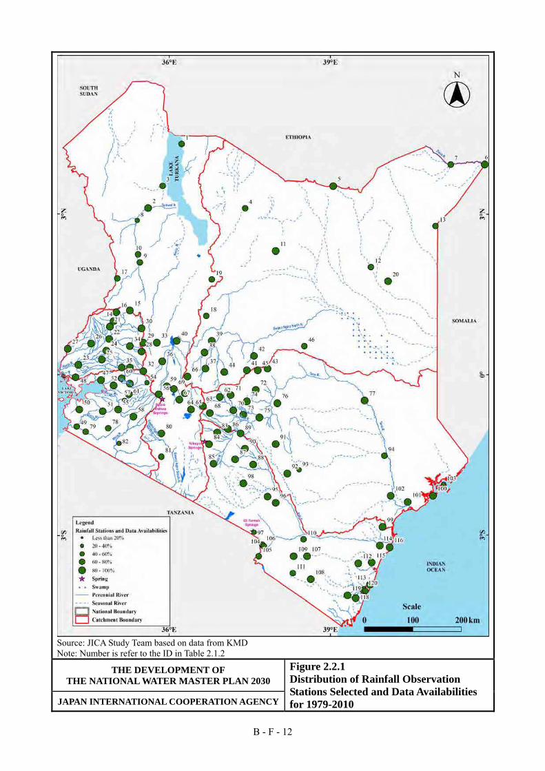
B - F - 12
Source: JICA Study Team based on data from KMD Note: Number is refer to the ID in Table 2.1.2
THE DEVELOPMENT OF THE NATIONAL WATER MASTER PLAN 2030
Figure 2.2.1 Distribution of Rainfall Observation Stations Selected and Data Availabilities for 1979-2010 JAPAN INTERNATIONAL COOPERATION AGENCY

B - F - 13
Source: JICA Study Team based on data from KMD
THE DEVELOPMENT OF THE NATIONAL WATER MASTER PLAN 2030
Figure 2.2.2 Mean Annual Rainfall for 1981 - 2010
JAPAN INTERNATIONAL COOPERATION AGENCY

B - F - 14
Source: JICA Study Team based on data from KMD
THE DEVELOPMENT OF THE NATIONAL WATER MASTER PLAN 2030
Figure 2.2.3 Mean Seasonal Rainfall for 1981 - 2010
JAPAN INTERNATIONAL COOPERATION AGENCY

B - F - 15
Source: JICA Study Team based on data from KMD
THE DEVELOPMENT OF THE NATIONAL WATER MASTER PLAN 2030
Figure 2.2.4 Mean Monthly Rainfall for 1981 - 2010
JAPAN INTERNATIONAL COOPERATION AGENCY

B - F - 16
Source: JICA Study Team based on data from KMD
THE DEVELOPMENT OF THE NATIONAL WATER MASTER PLAN 2030
Figure 2.2.5 Frequency Analysis of Daily Rainfall (1/3)
JAPAN INTERNATIONAL COOPERATION AGENCY

B - F - 17
Source: JICA Study Team based on data from KMD
THE DEVELOPMENT OF THE NATIONAL WATER MASTER PLAN 2030
Figure 2.2.5 Frequency Analysis of Daily Rainfall (2/3)
JAPAN INTERNATIONAL COOPERATION AGENCY

B - F - 18
Source: JICA Study Team based on data from KMD
THE DEVELOPMENT OF THE NATIONAL WATER MASTER PLAN 2030
Figure 2.2.5 Frequency Analysis of Daily Rainfall (3/3)
JAPAN INTERNATIONAL COOPERATION AGENCY

B - F - 19
Note: SLSC: Standard Least-Squares Criterion Source: JICA Study Team based on data from KMD
THE DEVELOPMENT OF THE NATIONAL WATER MASTER PLAN 2030
Figure 2.2.6 Distribution of 1-Day Probable Rainfall Intensity for 1981 - 2010
JAPAN INTERNATIONAL COOPERATION AGENCY

B - F - 20
Note: SLSC: Standard Least-Squares Criterion Source: JICA Study Team based on data from KMD
THE DEVELOPMENT OF THE NATIONAL WATER MASTER PLAN 2030
Figure 2.2.7 Distribution of the 3-Day Probable Rainfall Intensity for 1981 - 2010
JAPAN INTERNATIONAL COOPERATION AGENCY

B - F - 21
Note: SLSC: Standard Least-Squares Criterion Source: JICA Study Team based on data from KMD
THE DEVELOPMENT OF THE NATIONAL WATER MASTER PLAN 2030
Figure 2.2.8 Distribution of the 5-Day Probable Rainfall Intensity for 1981 - 2010
JAPAN INTERNATIONAL COOPERATION AGENCY

B - F - 22
Note: SLSC: Standard Least-Squares Criterion Source: JICA Study Team based on data from KMD
THE DEVELOPMENT OF THE NATIONAL WATER MASTER PLAN 2030
Figure 2.2.9 Annual Number of Rainy Days for 1981 - 2010
JAPAN INTERNATIONAL COOPERATION AGENCY

B - F - 23
Note: SLSC: Standard Least-Squares Criterion Source: JICA Study Team based on data from KMD
THE DEVELOPMENT OF THE NATIONAL WATER MASTER PLAN 2030
Figure 2.2.10 Seasonal Rainy Days for 1981 - 2010
JAPAN INTERNATIONAL COOPERATION AGENCY

B - F - 24
Source: JICA Study Team based on data from KMD
THE DEVELOPMENT OF THE NATIONAL WATER MASTER PLAN 2030
Figure 2.2.11 Annual Rainfall of 1/10 Drought Year (1984) for 1981 - 2000
JAPAN INTERNATIONAL COOPERATION AGENCY

B - F - 25
Source: JICA Study Team based on data from KMD
THE DEVELOPMENT OF THE NATIONAL WATER MASTER PLAN 2030
Figure 2.2.12 Seasonal Rainfall of 1/10 Drought Year
JAPAN INTERNATIONAL COOPERATION AGENCY

B - F - 26
[Selected Stations for Temperature Analysis]
[Selected Stations for Rainfall Analysis]
THE DEVELOPMENT OF THE NATIONAL WATER MASTER PLAN 2030
Figure 3.2.1 Selected Stations for Trend Analysis
JAPAN INTERNATIONAL COOPERATION AGENCY
Source: JICA Study Team Note: Number shown in both figure means the number of data available years.
(Bottom Figure) The number inside blanket is the period of 1920s to 2000s, and the other is the period of 1960s-2000s.
(85)
(85)
(76)
(74)
(72)
(83)
(83)
(67)
(78)

B - F - 27
Station ID Station Name 1967
1968
1969
1970
1971
1972
1973
1974
1975
1976
1977
1978
1979
1980
1981
1982
1983
1984
1985
1986
1987
1988
8635000 Lodwar Meteorological Station8639000 Moyale Met. Station8641000 Mandera Met Station8737000 Marsabit Met Station8840000 Wajir Met Station8937022 Laikipia Air Base9034025 Kisumu Meteorological Station9039000 Garissa Met Station9135001 Narok Meteorological Station9136208 Kabete Agromet Station9237000 Makindu Met. Station9240001 Lamu Meteorological Station9338001 Voi Meteorological Station9439021 Mombasa Port Reitz Airport
Station ID Station Name 1989
1990
1991
1992
1993
1994
1995
1996
1997
1998
1999
2000
2001
2002
2003
2004
2005
2006
2007
2008
2009
2010
Number ofYears
(>=80%)
8635000 Lodwar Meteorological Station 268639000 Moyale Met. Station 218641000 Mandera Met Station 238737000 Marsabit Met Station 158840000 Wajir Met Station 238937022 Laikipia Air Base 99034025 Kisumu Meteorological Station 189039000 Garissa Met Station 169135001 Narok Meteorological Station 189136208 Kabete Agromet Station 189237000 Makindu Met. Station 209240001 Lamu Meteorological Station 279338001 Voi Meteorological Station 319439021 Mombasa Port Reitz Airport 14
Legend
90% <= data availability80% <= data availability < 90%70% <= data availability < 80%60% <= data availability < 70%50% <= data availability < 60%40% <= data availability < 50% data availability < 40%
Source: JICA Study Team with original data from KMD
THE DEVELOPMENT OF THE NATIONAL WATER MASTER PLAN 2030
Figure 3.2.2 Availability of Temperature Data
JAPAN INTERNATIONAL COOPERATION AGENCY

B - F - 28
Station ID Station Name
1926
1927
1928
1929
1930
1931
1932
1933
1934
1935
1936
1937
1938
1939
1940
1941
1942
1943
1944
1945
1946
1947
1948
1949
1950
1951
1952
1953
1954
8635000 LODWAR METEOROLOGICAL STATION8639000 MOYALE MET. STATION8641000 MANDERA MET STATION8737000 MARSABIT MET STATION8840000 WAJIR MET STATION8934008 KITALE GLOUCESTER VALE ESTATE (Spl)8937022 LAIKIPIA AIR BASE9034025 KISUMU METEOROLOGICAL STATION9036017 NYERI MINISTRY OF WORKS (Spl)9036020 NAKURU RAILWAY STATION (Spl)9039000 GARISSA MET STATION9135001 NAROK METEOROLOGICAL STATION9136208 KABETE AGROMET STATION9237000 MAKINDU MET. STATION9240001 LAMU METEOROLOGICAL STATION9338001 VOI METEOROLOGICAL STATION9439021 MOMBASA PORT REITZ AIRPORT
Station ID Station Name
1955
1956
1957
1958
1959
1960
1961
1962
1963
1964
1965
1966
1967
1968
1969
1970
1971
1972
1973
1974
1975
1976
1977
1978
1979
1980
1981
1982
1983
8635000 LODWAR METEOROLOGICAL STATION8639000 MOYALE MET. STATION8641000 MANDERA MET STATION8737000 MARSABIT MET STATION8840000 WAJIR MET STATION8934008 KITALE GLOUCESTER VALE ESTATE (Spl)8937022 LAIKIPIA AIR BASE9034025 KISUMU METEOROLOGICAL STATION9036017 NYERI MINISTRY OF WORKS (Spl)9036020 NAKURU RAILWAY STATION (Spl)9039000 GARISSA MET STATION9135001 NAROK METEOROLOGICAL STATION9136208 KABETE AGROMET STATION9237000 MAKINDU MET. STATION9240001 LAMU METEOROLOGICAL STATION9338001 VOI METEOROLOGICAL STATION9439021 MOMBASA PORT REITZ AIRPORT
Station ID Station Name
1984
1985
1986
1987
1988
1989
1990
1991
1992
1993
1994
1995
1996
1997
1998
1999
2000
2001
2002
2003
2004
2005
2006
2007
2008
2009
2010
8635000 LODWAR METEOROLOGICAL STATION8639000 MOYALE MET. STATION8641000 MANDERA MET STATION8737000 MARSABIT MET STATION8840000 WAJIR MET STATION8934008 KITALE GLOUCESTER VALE ESTATE (Spl)8937022 LAIKIPIA AIR BASE9034025 KISUMU METEOROLOGICAL STATION9036017 NYERI MINISTRY OF WORKS (Spl)9036020 NAKURU RAILWAY STATION (Spl)9039000 GARISSA MET STATION9135001 NAROK METEOROLOGICAL STATION9136208 KABETE AGROMET STATION9237000 MAKINDU MET. STATION9240001 LAMU METEOROLOGICAL STATION9338001 VOI METEOROLOGICAL STATION9439021 MOMBASA PORT REITZ AIRPORT
Note: supplemental stations are marked with (Spl)
3931
31
Number ofYears
(>=80%)
8173516932804551
32
323932
32
75
Legend
90% <= data availability80% <= data availability < 90%70% <= data availability < 80%60% <= data availability < 70%50% <= data availability < 60%40% <= data availability < 50% data availability < 40%
Source: JICA Study Team with original data from KMD
THE DEVELOPMENT OF THE NATIONAL WATER MASTER PLAN 2030
Figure 3.2.3 Availability of Rainfall Data
JAPAN INTERNATIONAL COOPERATION AGENCY

B - F - 29
[Annual Mean Temperature] [Annual Mean Maximum Temperature]
[Annual Mean Minimum Temperature]
Source: JICA Study Team
THE DEVELOPMENT OF THE NATIONAL WATER MASTER PLAN 2030
Figure 3.3.1 Spatial Distribution of Temperature Trend
JAPAN INTERNATIONAL COOPERATION AGENCY
Source: JICA Study Team Note: Color of a zone is derived from average value of stations which are located in the zone. Gray color of
a zone means that there is no station in the zone.
Climate Zone Significant Trend
1.0 – 0.5 – 1.0 0.1 – 0.5
-0.1 – 0.1 -0.5 – -0.1 -1.0 – -0.5
– -1.0
Rate [degree per 20 years]
Legend
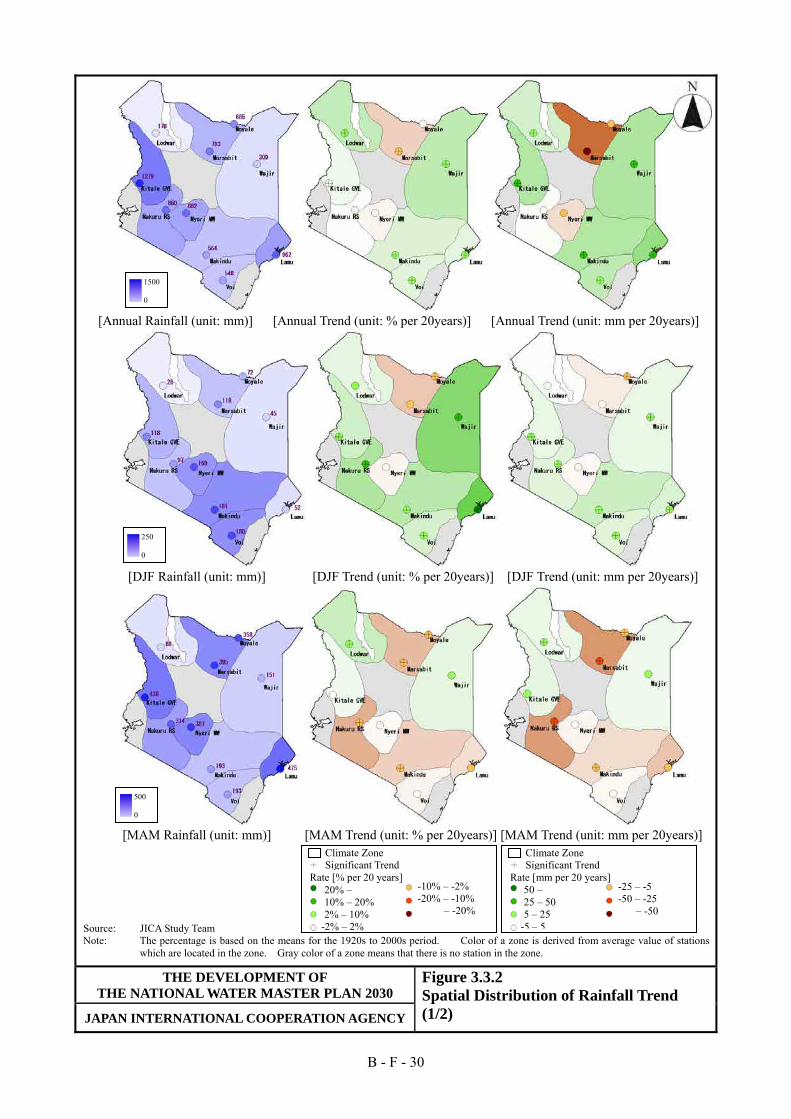
B - F - 30
[Annual Rainfall (unit: mm)] [Annual Trend (unit: % per 20years)] [Annual Trend (unit: mm per 20years)]
[DJF Rainfall (unit: mm)] [DJF Trend (unit: % per 20years)] [DJF Trend (unit: mm per 20years)]
[MAM Rainfall (unit: mm)] [MAM Trend (unit: % per 20years)] [MAM Trend (unit: mm per 20years)]
THE DEVELOPMENT OF THE NATIONAL WATER MASTER PLAN 2030
Figure 3.3.2 Spatial Distribution of Rainfall Trend (1/2) JAPAN INTERNATIONAL COOPERATION AGENCY
-10% – -2% -20% – -10%
– -20%
Climate Zone Significant Trend
Rate [% per 20 years] 20% – 10% – 20%2% – 10%
-2% – 2%
Climate Zone Significant Trend
Rate [mm per 20 years] 50 – 25 – 50 5 – 25
-5 – 5
-25 – -5 -50 – -25
– -50
1500 0
250 0
500 0
Source: JICA Study Team Note: The percentage is based on the means for the 1920s to 2000s period. Color of a zone is derived from average value of stations
which are located in the zone. Gray color of a zone means that there is no station in the zone.

B - F - 31
[JJA Rainfall (unit: mm)] [JJA Trend (unit: % per 20years)] [JJA Trend (unit: mm per 20years)]
[SON Rainfall (unit: mm)] [SON Trend (unit: % per 20years)] [SON Trend (unit: mm per 20years)]
[Rainy Days (unit: day)] [Rainy Days Trend (unit: % per 20years)] [Rainy Days Trend (unit: day per 20years)
THE DEVELOPMENT OF THE NATIONAL WATER MASTER PLAN 2030
Figure 3.3.2 Spatial Distribution of Rainfall Trend (2/2) JAPAN INTERNATIONAL COOPERATION AGENCY
Significant Trend Rate [mm per 20 years]
50 – 25 – 50 5 – 25
-5 – 5
-25 – -5 -50 – -25
– -50
Rate [day per 20 years] 10 – 5 – 10 1 – 5
-1 – 1
-5 – -1 -10 – -5
– -10
Climate Zone
-10% – -2% -20% – -10%
– -20%
Climate Zone Significant Trend
Rate [% per 20 years] 20% – 10% – 20% 2% – 10%
-2% – 2%
500 0
350 0
150 0
Source: JICA Study Team Note: The percentage is based on the means for the 1920s to 2000s period. Color of a zone is derived from average value of stations
which are located in the zone. Gray color of a zone means that there is no station in the zone.

B - F - 32
Correlation Root Mean Square Error
0
0.2
0.4
0.6
0.8
1
1.2
Jan Feb Mar Apr May Jun Jul Aug Sep Oct Nov Dec
correlation
Precipitation (pr)
giss‐aom
giss_model_e_r
0
0.5
1
1.5
2
2.5
3
3.5
4
4.5
5
Jan Feb Mar Apr May Jun Jul Aug Sep Oct Nov Dec
rmse
Precipitation (pr)
0
0.2
0.4
0.6
0.8
1
1.2
Jan Feb Mar Apr May Jun Jul Aug Sep Oct Nov Dec
correlation
Outgoing Longwave Radiation (olr)
iap_fgoals1_0_g
0
5
10
15
20
25
30
35
Jan Feb Mar Apr May Jun Jul Aug Sep Oct Nov Dec
rmse
Outgoing Longwave Radiation (olr)
0
0.2
0.4
0.6
0.8
1
1.2
Jan Feb Mar Apr May Jun Jul Aug Sep Oct Nov Dec
correlation
Sea Level Pressure (slp)
giss_model_e_r
ingv_echam4
miub_echo_g
0
1
2
3
4
5
6
7
Jan Feb Mar Apr May Jun Jul Aug Sep Oct Nov Dec
rmse
Sea Level Pressure (slp)
giss_model_e_r
0
0.2
0.4
0.6
0.8
1
1.2
Jan Feb Mar Apr May Jun Jul Aug Sep Oct Nov Dec
correlation
Surface Air Temperature (tas)
iap_fgoals1_0_g
0
1
2
3
4
5
6
7
8
9
Jan Feb Mar Apr May Jun Jul Aug Sep Oct Nov Dec
rmse
Surface Air Temperature (tas)
iap_fgoals1_0_g
csiro_mk3_5
Source: Analysis by JICA Study Team with the data provided by Kenya Meteorological Department, The Data Integration, and Analysis System (DIAS) dataset, and The Phase 3 of Coupled Model Intercomparison Project (CMIP3) multi-model dataset.
THE DEVELOPMENT OF THE NATIONAL WATER MASTER PLAN 2030
Figure 4.4.1 Evaluation of the Reproducibility of GCMs and Selection of the Appropriate Models JAPAN INTERNATIONAL COOPERATION AGENCY

B - F - 33
Note : OBS means Observation Source: Kenya Meteorological Department, The Data Integration and Analysis System (DIAS) dataset, and The Phase 3 of Coupled Model Intercomparison Project (CMIP3) multi-model dataset.
THE DEVELOPMENT OF THE NATIONAL WATER MASTER PLAN 2030
Figure 4.8.1 Spatial Distribution of Mean Annual Rainfall
JAPAN INTERNATIONAL COOPERATION AGENCY
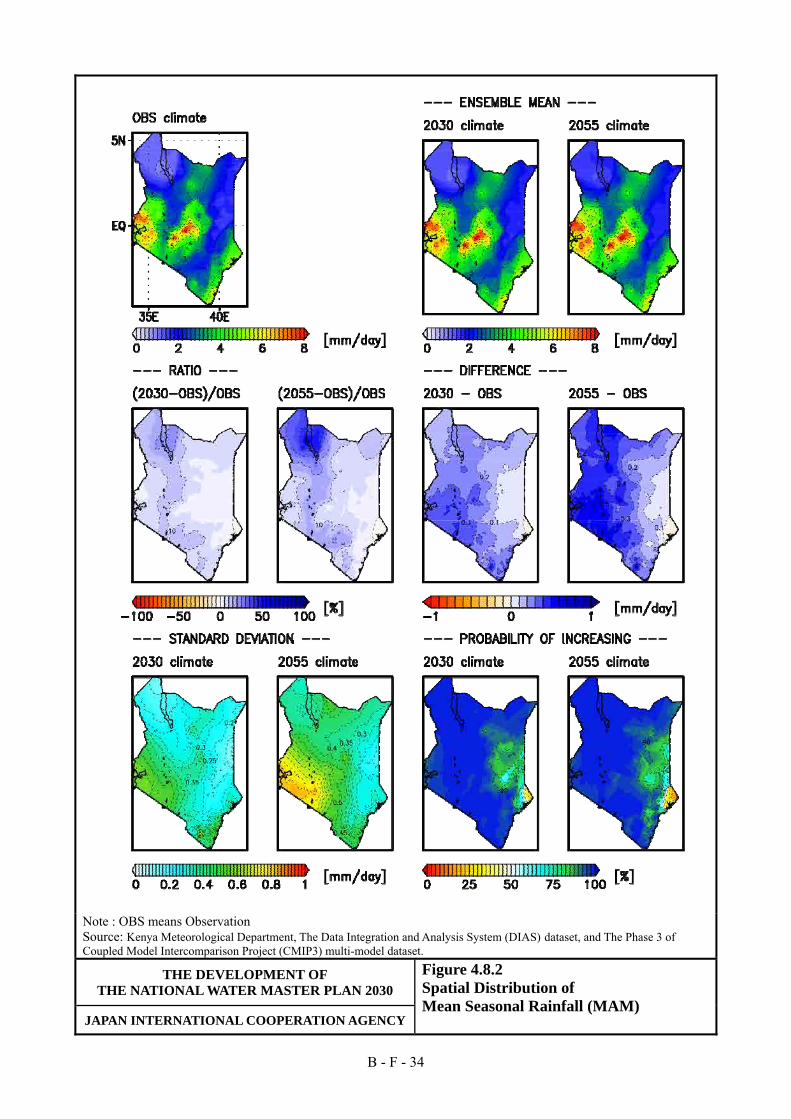
B - F - 34
Note : OBS means Observation Source: Kenya Meteorological Department, The Data Integration and Analysis System (DIAS) dataset, and The Phase 3 of Coupled Model Intercomparison Project (CMIP3) multi-model dataset.
THE DEVELOPMENT OF THE NATIONAL WATER MASTER PLAN 2030
Figure 4.8.2 Spatial Distribution of Mean Seasonal Rainfall (MAM)
JAPAN INTERNATIONAL COOPERATION AGENCY

B - F - 35
Note : OBS means Observation Source: Kenya Meteorological Department, The Data Integration and Analysis System (DIAS) dataset, and The Phase 3 of Coupled Model Intercomparison Project (CMIP3) multi-model dataset.
THE DEVELOPMENT OF THE NATIONAL WATER MASTER PLAN 2030
Figure 4.8.3 Spatial Distribution of Mean Seasonal Rainfall (JJA)
JAPAN INTERNATIONAL COOPERATION AGENCY

B - F - 36
Note : OBS means Observation Source: Kenya Meteorological Department, The Data Integration and Analysis System (DIAS) dataset, and The Phase 3 of Coupled Model Intercomparison Project (CMIP3) multi-model dataset.
THE DEVELOPMENT OF THE NATIONAL WATER MASTER PLAN 2030
Figure 4.8.4 Spatial Distribution of Mean Seasonal Rainfall (SON)
JAPAN INTERNATIONAL COOPERATION AGENCY

B - F - 37
Note : OBS means Observation Source: Kenya Meteorological Department, The Data Integration and Analysis System (DIAS) dataset, and The Phase 3 of Coupled Model Intercomparison Project (CMIP3) multi-model dataset.
THE DEVELOPMENT OF THE NATIONAL WATER MASTER PLAN 2030
Figure 4.8.5 Spatial Distribution of Mean Seasonal Rainfall (DJF)
JAPAN INTERNATIONAL COOPERATION AGENCY

B - F - 38
Note : OBS means Observation Source: Kenya Meteorological Department, The Data Integration and Analysis System (DIAS) dataset, and The Phase 3 of Coupled Model Intercomparison Project (CMIP3) multi-model dataset.
THE DEVELOPMENT OF THE NATIONAL WATER MASTER PLAN 2030
Figure 4.8.6 Spatial Distribution of Daily Rainfall Intensity for 10 years return period
JAPAN INTERNATIONAL COOPERATION AGENCY

B - F - 39
Note : OBS means Observation Source: Kenya Meteorological Department, The Data Integration and Analysis System (DIAS) dataset, and The Phase 3 of Coupled Model Intercomparison Project (CMIP3) multi-model dataset.
THE DEVELOPMENT OF THE NATIONAL WATER MASTER PLAN 2030
Figure 4.8.7 Spatial Distribution of Daily Rainfall Intensity for 50 years return period
JAPAN INTERNATIONAL COOPERATION AGENCY

B - F - 40
Note : OBS means Observation Source: Kenya Meteorological Department, The Data Integration and Analysis System (DIAS) dataset, and The Phase 3 of Coupled Model Intercomparison Project (CMIP3) multi-model dataset.
THE DEVELOPMENT OF THE NATIONAL WATER MASTER PLAN 2030
Figure 4.8.8 Spatial Distribution of Daily Rainfall Intensity for 100 years return period
JAPAN INTERNATIONAL COOPERATION AGENCY

B - F - 41
Note : OBS means Observation Source: Kenya Meteorological Department, The Data Integration and Analysis System (DIAS) dataset, and The Phase 3 of Coupled Model Intercomparison Project (CMIP3) multi-model dataset.
THE DEVELOPMENT OF THE NATIONAL WATER MASTER PLAN 2030
Figure 4.8.9 Spatial Distribution of Number of Rainy Days per Year
JAPAN INTERNATIONAL COOPERATION AGENCY

B - F - 42
Note : OBS means Observation Source: Kenya Meteorological Department, The Data Integration and Analysis System (DIAS) dataset, and The Phase 3 of Coupled Model Intercomparison Project (CMIP3) multi-model dataset.
THE DEVELOPMENT OF THE NATIONAL WATER MASTER PLAN 2030
Figure 4.8.10 Spatial Distribution of Number of Rainy Days per Season (MAM) JAPAN INTERNATIONAL COOPERATION AGENCY

B - F - 43
Source: Kenya Meteorological Department, The Data Integration and Analysis System (DIAS) dataset, and The Phase 3 of Coupled Model Intercomparison Project (CMIP3) multi-model dataset.
THE DEVELOPMENT OF THE NATIONAL WATER MASTER PLAN 2030
Figure 4.8.11 Spatial Distribution of Number of Rainy Days per Season (JJA)
JAPAN INTERNATIONAL COOPERATION AGENCY

B - F - 44
Source: Kenya Meteorological Department, The Data Integration and Analysis System (DIAS) dataset, and The Phase 3 of Coupled Model Intercomparison Project (CMIP3) multi-model dataset.
THE DEVELOPMENT OF THE NATIONAL WATER MASTER PLAN 2030
Figure 4.8.12 Spatial Distribution of Number of Rainy Days per Season (SON)
JAPAN INTERNATIONAL COOPERATION AGENCY

B - F - 45
Source: Kenya Meteorological Department, The Data Integration and Analysis System (DIAS) dataset, and The Phase 3 of Coupled Model Intercomparison Project (CMIP3) multi-model dataset.
THE DEVELOPMENT OF THE NATIONAL WATER MASTER PLAN 2030
Figure 4.8.13 Spatial Distribution of Number of Rainy Days per Season (DJF)
JAPAN INTERNATIONAL COOPERATION AGENCY

B - F - 46
Source: Kenya Meteorological Department, The Data Integration and Analysis System (DIAS) dataset, and The Phase 3 of Coupled Model Intercomparison Project (CMIP3) multi-model dataset.
THE DEVELOPMENT OF THE NATIONAL WATER MASTER PLAN 2030
Figure 4.8.14 Spatial Distribution of Mean Annual Rainfall of Drought Year for 10 years Return Period JAPAN INTERNATIONAL COOPERATION AGENCY

B - F - 47
Source: Kenya Meteorological Department, The Data Integration and Analysis System (DIAS) dataset, and The Phase 3 of Coupled Model Intercomparison Project (CMIP3) multi-model dataset.
THE DEVELOPMENT OF THE NATIONAL WATER MASTER PLAN 2030
Figure 4.8.15 Spatial Distribution of Mean Seasonal Rainfall of Drought Year for 10 Years Return Period (MAM) JAPAN INTERNATIONAL COOPERATION AGENCY

B - F - 48
Source: Kenya Meteorological Department, The Data Integration and Analysis System (DIAS) dataset, and The Phase 3 of Coupled Model Intercomparison Project (CMIP3) multi-model dataset.
THE DEVELOPMENT OF THE NATIONAL WATER MASTER PLAN 2030
Figure 4.8.16 Spatial Distribution of Mean Seasonal Rainfall of Drought Year for 10 Years Return Period (JJA) JAPAN INTERNATIONAL COOPERATION AGENCY

B - F - 49
Source: Kenya Meteorological Department, The Data Integration and Analysis System (DIAS) dataset, and The Phase 3 of Coupled Model Intercomparison Project (CMIP3) multi-model dataset.
THE DEVELOPMENT OF THE NATIONAL WATER MASTER PLAN 2030
Figure 4.8.17 Spatial Distribution of Mean Seasonal Rainfall of Drought Year for 10 Years Return Period (SON) JAPAN INTERNATIONAL COOPERATION AGENCY

B - F - 50
Source: Kenya Meteorological Department, The Data Integration and Analysis System (DIAS) dataset, and The Phase 3 of Coupled Model Intercomparison Project (CMIP3) multi-model dataset.
THE DEVELOPMENT OF THE NATIONAL WATER MASTER PLAN 2030
Figure 4.8.18 Spatial Distribution of Mean Seasonal Rainfall of Drought Year for 10 Years Return Period (DJF) JAPAN INTERNATIONAL COOPERATION AGENCY

B - F - 51
Source: Kenya Meteorological Department, The Data Integration and Analysis System (DIAS) dataset, and The Phase 3 of Coupled Model Intercomparison Project (CMIP3) multi-model dataset.
THE DEVELOPMENT OF THE NATIONAL WATER MASTER PLAN 2030
Figure 4.8.19 Spatial Distribution of Mean Annual Surface Air Temperature
JAPAN INTERNATIONAL COOPERATION AGENCY

B - F - 52
Source: Kenya Meteorological Department, The Data Integration and Analysis System (DIAS) dataset, and The Phase 3 of Coupled Model Intercomparison Project (CMIP3) multi-model dataset.
THE DEVELOPMENT OF THE NATIONAL WATER MASTER PLAN 2030
Figure 4.8.20 Spatial Distribution of Mean Seasonal Surface Air Temperature (MAM) JAPAN INTERNATIONAL COOPERATION AGENCY

B - F - 53
Source: Kenya Meteorological Department, The Data Integration and Analysis System (DIAS) dataset, and The Phase 3 of Coupled Model Intercomparison Project (CMIP3) multi-model dataset.
THE DEVELOPMENT OF THE NATIONAL WATER MASTER PLAN 2030
Figure 4.8.21 Spatial Distribution of Mean Seasonal Surface Air Temperature (JJA) JAPAN INTERNATIONAL COOPERATION AGENCY

B - F - 54
Source: Kenya Meteorological Department, The Data Integration and Analysis System (DIAS) dataset, and The Phase 3 of Coupled Model Intercomparison Project (CMIP3) multi-model dataset.
THE DEVELOPMENT OF THE NATIONAL WATER MASTER PLAN 2030
Figure 4.8.22 Spatial Distribution of Mean Seasonal Surface Air Temperature (SON) JAPAN INTERNATIONAL COOPERATION AGENCY

B - F - 55
Source: Kenya Meteorological Department, The Data Integration and Analysis System (DIAS) dataset, and The Phase 3 of Coupled Model Intercomparison Project (CMIP3) multi-model dataset.
THE DEVELOPMENT OF THE NATIONAL WATER MASTER PLAN 2030
Figure 4.8.23 Spatial Distribution of Mean Seasonal Surface Air Temperature (DJF) JAPAN INTERNATIONAL COOPERATION AGENCY

B - F - 56
Source: Kenya Meteorological Department, The Data Integration and Analysis System (DIAS) dataset, and The Phase 3 of Coupled Model Intercomparison Project (CMIP3) multi-model dataset.
THE DEVELOPMENT OF THE NATIONAL WATER MASTER PLAN 2030
Figure 4.9.1 Spatial Distribution of Mean Annual Potential Evapotranspiration (Hamon Method) JAPAN INTERNATIONAL COOPERATION AGENCY

B - F - 57
Source: Kenya Meteorological Department, The Data Integration and Analysis System (DIAS) dataset, and The Phase 3 of Coupled Model Intercomparison Project (CMIP3) multi-model dataset.
THE DEVELOPMENT OF THE NATIONAL WATER MASTER PLAN 2030
Figure 4.9.2Spatial Distribution of Mean Seasonal Potential Evapotranspiration (MAM, Hamon Method) JAPAN INTERNATIONAL COOPERATION AGENCY

B - F - 58
Source: Kenya Meteorological Department, The Data Integration and Analysis System (DIAS) dataset, and The Phase 3 of Coupled Model Intercomparison Project (CMIP3) multi-model dataset.
THE DEVELOPMENT OF THE NATIONAL WATER MASTER PLAN 2030
Figure 4.9.3Spatial Distribution of Mean Seasonal Potential Evapotranspiration (JJA, Hamon Method) JAPAN INTERNATIONAL COOPERATION AGENCY

B - F - 59
Source: Kenya Meteorological Department, The Data Integration and Analysis System (DIAS) dataset, and The Phase 3 of Coupled Model Intercomparison Project (CMIP3) multi-model dataset.
THE DEVELOPMENT OF THE NATIONAL WATER MASTER PLAN 2030
Figure 4.9.4Spatial Distribution of Mean Seasonal Potential Evapotranspiration (SON, Hamon Method) JAPAN INTERNATIONAL COOPERATION AGENCY

B - F - 60
Source: Kenya Meteorological Department, The Data Integration and Analysis System (DIAS) dataset, and The Phase 3 of Coupled Model Intercomparison Project (CMIP3) multi-model dataset.
THE DEVELOPMENT OF THE NATIONAL WATER MASTER PLAN 2030
Figure 4.9.5Spatial Distribution of Mean Seasonal Potentia Evapotranspiration (DEC, Hamon Method) JAPAN INTERNATIONAL COOPERATION AGENCY

B - F - 61
Source: Kenya Meteorological Department, The Data Integration and Analysis System (DIAS) dataset, and The Phase 3 of Coupled Model Intercomparison Project (CMIP3) multi-model dataset.
THE DEVELOPMENT OF THE NATIONAL WATER MASTER PLAN 2030
Figure 4.9.6Spatial Distribution of Mean Annual Potential Evapotranspiration (FAO Penman – Monteith Method) JAPAN INTERNATIONAL COOPERATION AGENCY

B - F - 62
Source: Kenya Meteorological Department, The Data Integration and Analysis System (DIAS) dataset, and The Phase 3 of Coupled Model Intercomparison Project (CMIP3) multi-model dataset.
THE DEVELOPMENT OF THE NATIONAL WATER MASTER PLAN 2030
Figure 4.9.7Spatial Distribution of Mean Seasonal Potential Evapotranspiration (MAM, FAO Penman – Monteith Method) JAPAN INTERNATIONAL COOPERATION AGENCY

B - F - 63
Source: Kenya Meteorological Department, The Data Integration and Analysis System (DIAS) dataset, and The Phase 3 of Coupled Model Intercomparison Project (CMIP3) multi-model dataset.
THE DEVELOPMENT OF THE NATIONAL WATER MASTER PLAN 2030
Figure 4.9.8Spatial Distribution of Mean Seasonal Potential Evapotranspiration (JJA, FAO Penman – Monteith Method)JAPAN INTERNATIONAL COOPERATION AGENCY

B - F - 64
Source: Kenya Meteorological Department, The Data Integration and Analysis System (DIAS) dataset, and The Phase 3 of Coupled Model Intercomparison Project (CMIP3) multi-model dataset.
THE DEVELOPMENT OF THE NATIONAL WATER MASTER PLAN 2030
Figure 4.9.9Spatial Distribution of Mean Seasonal Potential Evapotranspiration (SON, FAO Penman – Monteith Method) JAPAN INTERNATIONAL COOPERATION AGENCY

B - F - 65
Source: Kenya Meteorological Department, The Data Integration and Analysis System (DIAS) dataset, and The Phase 3 of Coupled Model Intercomparison Project (CMIP3) multi-model dataset.
THE DEVELOPMENT OF THE NATIONAL WATER MASTER PLAN 2030
Figure 4.9.10Spatial Distribution of Mean Seasonal Potentia Evapotranspiration (DJF, FAO Penman – Monteith Method) JAPAN INTERNATIONAL COOPERATION AGENCY

B - F - 66
Source: Kenya Meteorological Department, The Data Integration and Analysis System (DIAS) dataset, and The Phase 3 of Coupled Model Intercomparison Project (CMIP3) multi-model dataset.
THE DEVELOPMENT OF THE NATIONAL WATER MASTER PLAN 2030
Figure 4.9.11 Spatial Distribution of Mean Annual P-PET (Hamon Method) JAPAN INTERNATIONAL COOPERATION AGENCY

B - F - 67
Source: Kenya Meteorological Department, The Data Integration and Analysis System (DIAS) dataset, and The Phase 3 of Coupled Model Intercomparison Project (CMIP3) multi-model dataset.
THE DEVELOPMENT OF THE NATIONAL WATER MASTER PLAN 2030
Figure 4.9.12 Spatial Distribution of Mean Seasonal P-E (MAM, Hamon Method) JAPAN INTERNATIONAL COOPERATION AGENCY

B - F - 68
Source: Kenya Meteorological Department, The Data Integration and Analysis System (DIAS) dataset, and The Phase 3 of Coupled Model Intercomparison Project (CMIP3) multi-model dataset.
THE DEVELOPMENT OF THE NATIONAL WATER MASTER PLAN 2030
Figure 4.9.13 Spatial Distribution of Mean Seasonal P-E (JJA, Hamon Method) JAPAN INTERNATIONAL COOPERATION AGENCY

B - F - 69
Source: Kenya Meteorological Department, The Data Integration and Analysis System (DIAS) dataset, and The Phase 3 of Coupled Model Intercomparison Project (CMIP3) multi-model dataset.
THE DEVELOPMENT OF THE NATIONAL WATER MASTER PLAN 2030
Figure 4.9.14 Spatial Distribution of Mean Seasonal P-PET (SON, Hamon Method) JAPAN INTERNATIONAL COOPERATION AGENCY

B - F - 70
Source: Kenya Meteorological Department, The Data Integration and Analysis System (DIAS) dataset, and The Phase 3 of Coupled Model Intercomparison Project (CMIP3) multi-model dataset.
THE DEVELOPMENT OF THE NATIONAL WATER MASTER PLAN 2030
Figure 4.9.15 Spatial Distribution of Mean Seasonal P-PET (DJF, Hamon Method) JAPAN INTERNATIONAL COOPERATION AGENCY

B - F - 71
Source: Kenya Meteorological Department, The Data Integration and Analysis System (DIAS) dataset, and The Phase 3 of Coupled Model Intercomparison Project (CMIP3) multi-model dataset.
THE DEVELOPMENT OF THE NATIONAL WATER MASTER PLAN 2030
Figure 4.9.16 Spatial Distribution of Mean Annual P-PET (FAO Penman – Monteith Method) JAPAN INTERNATIONAL COOPERATION AGENCY

B - F - 72
Source: Kenya Meteorological Department, The Data Integration and Analysis System (DIAS) dataset, and The Phase 3 of Coupled Model Intercomparison Project (CMIP3) multi-model dataset.
THE DEVELOPMENT OF THE NATIONAL WATER MASTER PLAN 2030
Figure 4.9.17 Spatial Distribution of Mean Seasonal P-PET (MAM, FAO Penman – Monteith Method) JAPAN INTERNATIONAL COOPERATION AGENCY

B - F - 73
Source: Kenya Meteorological Department, The Data Integration and Analysis System (DIAS) dataset, and The Phase 3 of Coupled Model Intercomparison Project (CMIP3) multi-model dataset.
THE DEVELOPMENT OF THE NATIONAL WATER MASTER PLAN 2030
Figure 4.9.18 Spatial Distribution of Mean Seasonal P-PET (JJA, FAO Penman – Monteith Method) JAPAN INTERNATIONAL COOPERATION AGENCY

B - F - 74
Source: Kenya Meteorological Department, The Data Integration and Analysis System (DIAS) dataset, and The Phase 3 of Coupled Model Intercomparison Project (CMIP3) multi-model dataset.
THE DEVELOPMENT OF THE NATIONAL WATER MASTER PLAN 2030
Figure 4.9.19 Spatial Distribution of Mean Seasonal P-PET (SON, FAO Penman – Monteith Method) JAPAN INTERNATIONAL COOPERATION AGENCY

B - F - 75
Source: Kenya Meteorological Department, The Data Integration and Analysis System (DIAS) dataset, and The Phase 3 of Coupled Model Intercomparison Project (CMIP3) multi-model dataset.
THE DEVELOPMENT OF THE NATIONAL WATER MASTER PLAN 2030
Figure 4.9.20 Spatial Distribution of Mean Seasonal P-PET (DJF, FAO Penman – Monteith Method) JAPAN INTERNATIONAL COOPERATION AGENCY