SECTORAL SHIFTS AND CYCLICAL UNEMPLOYMENT A RECONSIDERATION

THOMAS 1. PALLEY*

The debate over the relative importance of sectoral and aggregate shocks in explain- ing fluctuations in the aggregate unemployment rate has centered on the relationship between unemployment, job vacancies, and the dispersion of sectoral employment growth rates (which proxies for sectoral shocks). This paper examines some possible theoretical relationships between these variables, and, after decomposing unemploy- ment into components attributable to sectoral and aggregate shocks, estimates the importance of each. It finds that fluctuations in unemployment are principally caused by aggregate shocks, but sectoral shifts explain a significant, albeit steady, amount of unemployment.

I. INTRODUCTION

In a controversial paper Lillien [1982] argued that much 'of the rise in aggregate unemployment experienced in the 1970s and 1980s was attributable to increases in the natural rate of unemployment. These increases, he said, arose from shifts of demand between the different sectors of the national economy. These demand shifts increased unemployment because labor market frictions prevented the im- mediate reallocation of workers from de- clining sectors to expanding sectors. Lillien used a dispersion index of sectoral employment growth rates as a proxy for the extent of sectoral shifts and found that aggregate unemployment could be ex- plained by this dispersion with a positive distributed lag.

Given the much discussed changing composition of output and employment in the U.S., this interpretation of unemploy- ment quickly won adherents, such as Barro [1984]. More recent work by Abra- ham and Katz [1986] challenges this view. They argue that the rise in aggregate un-

Assistant Professor, New School for Social Re- search, New York.

employment was attributable to aggregate demand disturbances. They showed that if sectors had different cyclical sensitivi- ties, aggregate demand disturbances (such as those resulting from monetary policy or fluctuations in "animal spirits") could produce counter-cyclical fluctuations in the dispersion of sectoral employment growth rates. The finding that unemploy- ment was a distributed lag of this disper- sion did not, therefore, distinguish be- tween the two hypotheses. Instead, Abra- ham and Katz found vacancy rates to be negatively related to dispersion with a distributed lag. They interpreted this re- sult as confirmation of the aggregate de- mand hypothesis since it was consistent with a movement along the Beveridge curve?

My paper further explores the relation- ships between sectoral shifts, aggregate unemployment and aggregate vacancies. The theoretical section demonstrates that sectoral shifts are also consistent with a movement along the Beveridge curve and

1. The Beveridge Curve describes the relationship between vacancies and the rate of unemployment.

Economic Inquiry Vol. XXX, January 1992,1.17-133

117

@Western Economic Association International

118 ECONOMIC INQUIRY

a negative relation between vacancies and the dispersion of sectoral employment growth rates. This result potentially inval- idates Abraham and Katz’s claim, and at the same time provides a novel explana- tion of the Beveridge curve. In the empir- ical section I use the implications of the two hypotheses to decompose the disper- sion of sectoral employment growth rates into parts attributable to sectoral shifts and aggregate shocks respectively. These new measures are then used to estimate the relative contributions of sectoral shifts and aggregate disturbances to aggregate unemployment.

This paper is linked to an emerging literature on the sources of macroeco- nomic fluctuations. The seminal paper by Long and Plosser [1983] showed how real business cycle models could explain co- movements of output across sectors on the basis of sector-specific shocks. In a subse- quent paper Long and Plosser [1987] sought to identify the relative importance of aggregate versus sector specific shocks. Using a single-factor model of output growth, they found that aggregate shocks explained only a relatively small amount of the covariation of output across sectors, and concluded that sectoral shocks are largely responsible for cyclical fluctua- tions. Norrbin and Schlagenhauf [1988; 19911 continued this line of research, but allowed for multiple factors. In addition, they sought to quantify the relative signif- icance of sectoral versus aggregate shocks by decomposing the forecast error vari- ance for individual industries into compo- nents explained by the aggregate and sectoral factors. My current paper is dis- tinguished from previous research in both focus and methodology. First, I focus on the evolution of the aggregate rate of un- employment rather than the rate of output growth. Second, rather than adopting a VAR approach and decomposing forecast error variances, I attempt to explain the evolution of aggregate unemployment using a summary measure of sectoral

shifts introduced by Lillien [1982], but with important innovations in the measure’s construction.

Finally, the empirical decomposition of unemployment into parts attributable to sectoral and aggregate shocks is of consid- erable significance from a policy stand- point. If cyclical fluctuations in unemploy- ment are largely attributable to sectoral shocks, this implies that increases in the unemployment rate represent increases in the non-accelerating inflation rate of un- employment (NAIRU), with depressed sectors characterized by high unemploy- ment and booming sectors characterized by bottlenecks. In this case, attempts to reduce unemployment with macroeco- nomic measures are likely to have signifi- cant inflation costs. In contrast, if aggre- gate shocks explain cyclical fluctuations in the unemployment rate, this leaves open the possibility of a non-inflationary stabi- lization policy.

II. THE COMPETING THEORETICAL MODELS

The sectoral shift hypothesis Lillien’s model is derived from an ear-

lier paper by Lucas and Prescott [1974] in which imperfect information concerning the location of new jobs gives rise to search unemployment. The logic of the model is easily illustrated. Aggregate un- employment, U , evolves according to

u, = u,, + s, - I f t ,

where S, = current period separations, H, = current period hires.

Separations are assumed to depend on the extent of demand shifts between sectors. These shifts may be summarized by the statistic ut which measures the dispersion of sectoral demand shocks. Thus

S’ > 0.

PALLEY: CYCLICAL UNEMPLOYMENT 119

Finally, new hires are assumed to be a con- stant proportion (k > 0) of last period's un- employment so that

Solving the model given by equations (1)- (3) yields expected equilibrium unemploy- ment of

(4) U* = S ( Z ) / k ,

where Z equals the expected dispersion of sectoral demand shocks. Temporary in- creases in the dispersion of sectoral de- mand disturbances (ot > 5) resulting from adverse random sectoral demand shocks can cause temporary increases in unem- ployment above U*. If the increase in dis- persion is permanent, owing to a change in the probability distribution governing sectoral demand shocks, this will cause a permanent increase in U*.

In order to test for the effect of sectoral shifts on aggregate unemployment, Lillien created a proxy statistic for ut given by

n A ( ~ t = [ C Si,Xgi,t - g t ~ ~ I " ,

i-1 (5)

where n = s. =

t,t

gi,t =

8, =

the number of sectors share of ith sector employment in total employment, rate of growth of employment the ith sector, rate of growth of aggregate employment.

A Lillien then used ut as an explanatory vari- able in regressions of the aggregate rate of unemployment and found it to have con- siderable explanatory power.

For current empirical purposes, the sig- nificant implication is that employment growth in an individual sector is deter- mined mainly by the underlying sector

trend combined with a random sector dis- turbance. Additionally, if there are convex firm-level costs of adjusting employment, past sector employment growth will help predict current sector employment growth since firms will smooth expansions and contractions of their workforces.

The aggregate disturbance hypothesis Abraham and Katz [1986] challenge this

explanation of dispersion in sectoral em- ployment growth rates. They argue that the observed values of ot can also be explained by aggregate disturbances (they emphasize aggregate demand distur- bances) if sectors differ in their sensitivity to aggregate disturbances. In this model employment in each sector is determined according to

(6) In Ni,t = q,,i + al,iT + a2,dln Yt - lnY;),

where Ni,t = the level of employment in the ith sector,

T = time trend, Y t = actual GNP,

Y; = trend GNP,

In = natural log.

Then, for a two-sector model (i = 1,2) in which = employment growth dis- persion is defined as

Assuming the two sectors are initially equal in size, Nl,t=N2,t, this is approxi- mately equal to

120 ECONOMIC INQUIRY

In this case if - u ~ , ~ ) < 0, which implies that industry 2 is cyclically more sensitive than industry 1, the second term is posi- tive when actual GNP is below trend and negative when it is above. The variable crt can therefore exhibit counter-cyclical variation.

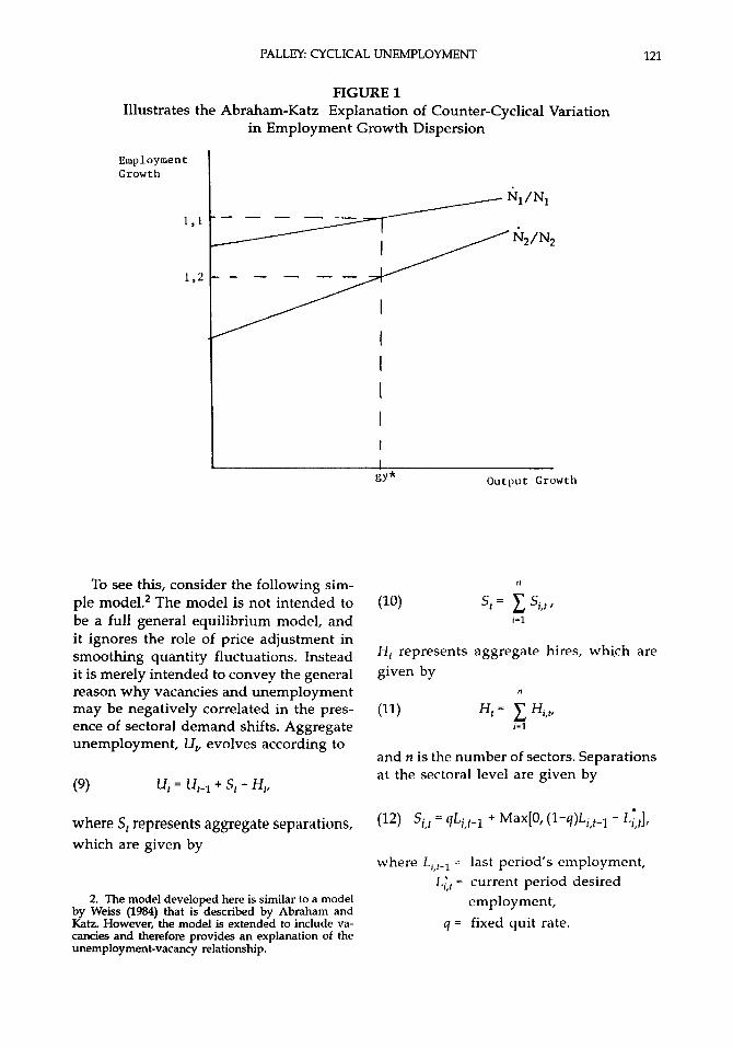
The Abraham-Katz hypothesis is illus- trated in Figure 1, which shows employ- ment growth plotted against output growth. Point gy* represents the underly- ing growth of potential output. If output growth is greater than gy*, the dispersion of employment growth across sectors nar- rows. Conversely, if output growth is less than gy*, the dispersion widens. Putting the pieces together, the evolution of unem- ployment is explained as follows. As the economy enters recession, output growth drops below potential, dispersion widens, and unemployment starts to rise. As the economy exits recession, output growth increases above potential, dispersion nar- rows, and unemployment starts to fall. Finally, for the purposes of this paper, the significant implication of the aggregate demand hypothesis is that employment growth in an individual sector is ex- plained by its own trend and its sensitivity to aggregate demand shocks. Essentially, the model is a single-factor model, and this factor affects all sectors in differing degrees. Thus contemporaneous employ- ment growth in the rest of the economy will predict employment growth in an individual sector, and can therefore serve to proxy for the unobserved aggregate demand shock. Lastly, if there are convex costs of adjusting employment, firms will smooth changes in their workforces and aggregate disturbances will have a lagged effect on unemployment.

To test between these competing hypotheses concerning the determination of of, Abraham and Katz turned to the relationship between unemployment and vacancies (proxied by the help wanted index). Under the sectoral shift hypothe-

sis, they argued, there should be a positive relationship between unemployment and vacancies, and uf should have a positive coefficient when used as an explanatory variable in regressions explaining vacan- cies. This is because shifts of demand cause increased job opportunities in sec- tors receiving positive shocks, which re- main unfilled because of worker igno- rance about the location of jobs or other labor market imperfections. In contrast the aggregate disturbance approach implies that unemployment and vacancies should be negatively correlated, and of should have a negative coefficient in vacancy re- gressions since increases in of are associ- ated with aggregate output being below trend. Abraham and Katz found the latter to be the case in their vacancy regressions for both U.S. and British data, and they interpreted this finding as a rejection of the sectoral shift hypothesis.

Critique of the Abraham-Katz Hypothesis The central piece of evidence which

Abraham and Katz used to reject the secto- ral shift hypothesis was that job vacancies (proxied by the ratio of the help wanted index to total non-agricultural employ- ment) were negatively correlated with the dispersion of sectoral employment growth rates. Abraham and Katz interpreted this negative correlation as indicative of a movement along the Beveridge curve, which they claimed was consistent with the aggregate demand hypothesis. In con- trast, they state, the sectoral shift hypoth- esis implies a positive correlation between vacancies and unemployment reflecting an outward expansion of the Beveridge curve. However, I argue below that a neg- ative correlation between vacancies and unemployment is also consistent with the sectoral shift hypothesis if it is costly to hire new workers. This possibility under- mines Abraham and Katz’s claim to have unambiguously disproved the sectoral shift hypothesis.

PALLEY CYCLICAL UNEMPLOYMENT 121

FIGURE 1 Illustrates the Abraham-Katz Explanation of Counter-Cyclical Variation

in Employment Growth Dispersion

Employment Growth

To see this, consider the following sim- ple modeL2 The model is not intended to be a full general equilibrium model, and it ignores the role of price adjustment in smoothing quantity fluctuations. Instead it is merely intended to convey the general reason why vacancies and unemployment may be negatively correlated in the pres- ence of sectoral demand shifts. Aggregate unemployment, U,, evolves according to

(9) u, = q-1 + s, - H ,

where S , represents aggregate separations, which are given by

2. The model developed here is similar to a model by Weiss (1984) that is described by Abraham and Katz. However, the model is extended to include va- cancies and therefore provides an explanation of the unemployment-vacancy relationship.

n

H , represents aggregate hires, whi,ch are given by

n

and n is the number of sectors. Separations at the sectoral level are given by

where = last period’s employment,

employment, Lit = current period desired

q = fixed quit rate.

122 ECONOMIC INQUIRY

When it comes to lay-offs, firms are as- sumed to adjust immediately to their de- sired w~rkforce .~ Total separations consist of quits and lay-offs (if positive). Hires at the sectoral level are given by

where A,, = current period job applicants,

Vi,t = current period vacancies.

Current period applicants are given by

increase with the size of the addition.* The condition 0 < a < 1 ensures that vacancies are non-negative and that vacancies are less than the gap between desired and ex- isting employment, i.e., the firm does not overshoot in its hiring. From (15) it then follows that if desired employment ex- pands, firms increase their advertised va- cancies. However, the actual adjustment to the desired level of employment is smoothed over a number of periods so that vacancies only increase a little ini- tially.

Now let desired employment in each sector evolve according to

Thus last periods unemployed are evenly spread across all sectors of the economy to become this period’s job applicants. This is the same labor allocation mecha- nism as in Lucas and Prescott [1974]. Job vacancies are given by

(15)

v, =

‘0

O < a < l .

The logic of this rule is as follows. Vacan- cies are zero if this periods desired labor force, L;, is less than the existing labor force (l-9)L,-1. If the desired labor force ex- ceeds the existing labor force, firms re- place current period quits and there is an additional partial adjustment. The partial adjustment term reflects the fact that it is costly to add new workers, and these costs

3. The assumption of costless layoffs is extreme. If there are some convex costs to layoffs, they will be smoothed. For purposes of the current argument all that is required is that layoff adjustments be more rapid than new hires. This is most easily managed by assuming instant layoffs.

where ei,f is a random sectoral demand shock distributed in some unspecified way and has a zero mean. In this case, should a sector receive a negative demand shock, vacancies in that sector may drop to zero, and there is no need even to ad- vertise to replace normal quits. At the same time other sectors hit with positive demand shocks will increase the level of their advertised vacancies. However, be- cause of the partial adjustment mecha- nism governing additions to employment, this increase may not offset the decline in vacancies elsewhere. As a result, aggregate vacancies fall. The net effect is that aggre- gate unemployment rises while aggregate vacancies fall. Sectoral shifts in the pres- ence of asymmetric hiring and firing costs can, therefore, trace out a Beveridge curve and explain movements along it.5

4. The vacancy rule given by equation (15) may be interpreted as an approximation to an optimal adjust- ment rule in the presence of zem firing costs and con- vex hiring costs. The one complication which is not accounted for is that if the current labor force were greater than the desired labor force the firm might still hire additional (temporarily surplus) workers so as to save a little next period when it anticipates replacing quits.

5. Asymmetric hiring and firing costs therefore provide a novel explanation of the Beveridge curve. This explanation complements a recent search theoretic explanation advanced by Blanchard and Diamond [1989].

PALLEY: CYCLICAL UNEMPLOYMENT 123

The relative size of industries may also matter. Suppose costs of hiring are a de- creasing function of existing size.6 Then, if sectors receiving negative shocks are large mature industries, while sectors receiving positive shocks are small emerging indus- tries, the drop in vacancies may be sub- stantial in absolute size in the mature sector and outweigh the smaller absolute gain in the emergent sector.

Lastly, if firms receiving negative de- mand shocks hoard labor because they know they will have to replace future costly quits, then vacancies at these firms will be zero for some time after. This means that sectoral shifts may have a negative influence on vacancies for a num- ber of periods.

Given the above description of hiring and firing behavior, a shift of demand between sectors instantaneously raises ag- gregate unemployment and depresses ag- gregate vacancies. Vacancies remain low for a number of periods, while unemploy- ment is high for a number of periods as growing industries gradually absorb the laid-off workers. There is some empirical support for this asymmetric pattern of employment adjustment. Neftci [1984] shows that increases in unemployment tend to be characterized by sudden jumps, while decreases involve gradual drops spread over a longer duration. This pat- tern is consistent with underlying firm behavior involving immediate layoffs and smoothed hiring.

111. THE RELATIVE IMPACT OF SECTORAL SHIFTS AND AGGREGATE DISTURBANCES:

AN ECONOMETRIC MODEL

The above discussion shows that the correlation between vacancies and the dis- persion of employment growth cannot be used to distinguish between the sectoral shifts and aggregate disturbance hypothe-

6. This is a standard argument in the investment literature.

ses. This is because both the sectoral shifts hypothesis and the aggregate disturbance hypothesis can predict a negative relation- ship between vacancies and the dispersion of sectoral employment growth. There- fore, the method adopted in the current paper is to decompose the dispersion of sectoral employment growth into a part attributable to sectoral factors and a part attributable to aggregate factors. I then use these separate measures to identify the relative contributions of sectoral and ag- gregate disturbances in explaining the rate of aggregate unemployment.

I used the following procedure for con- structing the decomposed measures of em- ployment growth dispersion. First, a re- gression was run determining the evolu- tion of employment growth in each indi- vidual sector:

4

4

C '3,t-j g-i,t-j + e;,t j-0

+

where = rate of employment growth in the ith sector,

g-i,t = rate of aggregate employment growth excluding sector i,

T = time trend, q t = residual.

All growth rates were computed using the first difference of the natural log. The vari- able g-i,t was defined as follows:

where Nt = aggregate employment, N j , t = employment in the ith

sector.

Equation (17) is a critical building block of the empirical model. Its purpose is to

124 ECONOMIC INQUIRY

identify that part of a sector's employment growth which is attributable to sector-spe- cific factors, and that part attributable to aggregate factors. The logic of this proce- dure is based on the inferential assump- tions that underlie the Granger-causality literature. Thus aggregate influences were accounted for by looking at employment growth in the rest of the economy: to the extent that employment growth in an in- dividual sector was Granger-caused by growth in the rest of the economy this suggests the influence of aggregate forces. The effects of contemporaneous aggregate disturbances were accounted for by in- cluding the current rate of employment growth in the rest of the economy as an independent variable.

Analogously, to capture sector-specific factors I looked at the extent to which lagged sectoral employment growth Granger-caused current sectoral employ- ment growth. Additionally, the effect of contemporaneous sector-specific distur- bances were accounted for by treating the residual as part of the sector-specific com- ponent. Finally, note that the definition of the aggregate rate of employment growth given by (18) ensures the removal of any direct influence of the dependent variable in (17) on the rate of aggregate employ- ment growth.

One caveat regarding the above meth- odology relates to the possibility of incor- rectly attributing causality if there are con- temporaneous spill-overs between sectors. In the current application, if there are strong within-quarter inter-sectoral multi- pliers, sector specific shocks could have an immediate effect on output and employ- ment in the rest of the economy. In this case, given the specification of equation (17), such shocks might be incorrectly counted as part of the aggregate factor, g-i,t. In effect, there is a possible problem of simultaneity bias with the left- hand- side variable impacting the right-hand- side regressor. To address this problem, equation (17) was estimated using the

Fair[1970] two-stage least squares estima- tor. The instruments for g-i,t were the cur- rent and four lagged values of the three- month treasury bill, and four lagged val- ues of aggregate output growth. The use of the treasury bill rate as an instrument reflects the belief that monetary policy targets short-term interest rates, so that they are therefore exogenous. Aggregate output growth was computed in a manner analogous to equation (18).

Having estimated (17) for each sector, the next step involved decomposing the rate of employment growth in each sector into a part attributable to sector specific and sectoral shift factors, and that part attributable to aggregate factors. The com- ponent attributable to sectoral influences was defined as

4

while the component attributable to ag- gregate influences was given by

4

x. i , t = C '3,'-j g-i,t-j.

j-0

Using equation (19) the dispersion in sectoral employment growth rates attrib- utable to sectoral influences was calcu- lated as

n

share of ith sector employment in total employment, average employment growth attributable to sectoral influences. was computed as

n

PALLEY CYCLICAL UNEMPLOYMENT 125

The dispersion in sectoral employment growth rates attributable to aggregate in- fluences was calculated as

n

i-I

where 57, = average employment growth attributable to aggregate influences.

X , was computed as

n

~

i-1

The variables crz,t and ux,t bear the follow- ing interpretations. uz,t captures the dis- persion in employment growth rates aris- ing from pure sectoral influences which were relevant for the sectoral shift hypoth- esis. captures the influence of aggre- gate disturbances on sectoral employment growth rates which were relevant to the aggregate disturbance hypothesis.

The variables az,, and ax,t were then used in regressions of aggregate unem- ployment given by

(25) U, = co = clTime + c2 U,-,

3 3

+ C ~ 3 , t - i ux,t-i + C ~ 4 , t - i *Z,t-i + e2,t. i-0 i-0

The coefficients attaching to uz and ux re- veal the relative sensitivity of aggregate unemployment to sectoral shifts and ag- gregate dist~rbances.~

7. The regression given by equation (25) differs from that used by Lillien and by Abraham and Katz not only in its decomposition of the dispersion vari- able, but also in its exclusion of an unanticipated mon- etary policy variable. The inclusion of this variable would be important if one were interested in construct- ing a series for the natural rate and subscribed to the anticipated policy ineffectiveness proposition.

IV. THE DATA AND RESULTS

The data used for estimating the model are from the Citibase Data Bank and were quarterly and seasonally adjusted. The sample period was 1948:111-1988:11. Two- stage least squares regressions of equation (17) were run for the eleven different sec- tors into which aggregate non-agricultural employment is decomposed: the results are shown in Table I. These results were then used to compute values of ux and uz per the formulae in (21)-(24). These constructed variables were, in turn, used in estimating equation (25) to estimate the effect of dispersion in sectoral employ- ment growth rates on aggregate unem- ployment.

The results of these further regressions are shown in Table 11. A number of differ- ent functional specifications, including log and semi-log transformations, were esti- mated to test for any non-linearities in the relationship, but only the simple linear form is reported. All regressions were es- timated using a maximum likelihood pro- cedure with a correction for second-order serial correlation. The coefficients of ox are negative. This suggests, contrary to Abra- ham and Katz, that positive aggregate disturbances cause the dispersion of secto- ral employment growth to widen. Three out of four coefficients for oz are positive, with the current and once lagged values having large and statistically significant coefficients. This pattern of signing con- firms the hypothesis that sectoral shifts raise unemployment.

The dispersion variables, ux and uz are generated regressors. Pagan [1984] ex- plains why the standard errors obtained from single-stage estimates using such re- gressors may be inconsistent. In the cur- rent application, the generation of ux per equation (17) involves the contemporane- ous rate of growth of aggregate employ- ment, and this variable may be correlated with the error term in equation (25). To correct for this problem, equation (25) was

126 ECONOMIC INQUIRY

TABLE I Estimates of sectoral employment growth per equation (17)

Mining Construction Durables Non-durables Transport/Util.

C

g(t-3,i)

Adj. R2

S.E.E.

-.on (-1.52)

.022

.004 C34)

(-04)

(W

(.31)

C33)

C39)

C91)

.007

.003

.003

.550

1.244

-1.487 (-1.65)

1.661 (1.92)

-.628 (-.91)

.053

.037

-.003 (-.87) -.016

(-.61)

.209 (2.33)

.061 (.70) -.059

(-.63)

.160 (1.91)

2.119 (3.54)

(-.33) -.169

-.488 (-1.33)

-.459 (-1.36)

.348 (1.14)

.391

.015

-.006 (-2.19)

-.073 (-3.12)

.lo4 (1.14)

.078 (34)

(.73) .062

-.026 (-.32)

3.769 (6.24)

-.158

-.022 (-.05)

-.477 (-1.04)

-.390

(-.94)

(-1.10)

.702

.012

-.004 (-2.65)

-.020 (-1.83)

.304 (3.22)

-.276 (-2.88)

-.079 (-.83)

-.020 (-.22)

1.373 (6.21)

-.674 (-3.27)

.458 (2.76)

-.264 (-1.75)

-.098 (-.79)

.589

.006

-.009 (-5.23)

.355 (2.75)

-.327 (-3.82)

-.089 (-.94)

-.006 (-.06)

-.030 (-.42)

.473 (1.96)

.771 (3.08)

.048 (.28) .320

(1.82)

-.044 (-.30)

.584

.007

Note: The sample period was 1948:III-1988:11. Figures in parentheses are t-statistics.

re-estimated using the Fair [1970] two- stage least squares estimator with a correc- tion for second-order serial correlation.8 The estimates obtained from this proce- dure are shown in the right-hand column of table (2). The results from these two- stage estimates are fully consistent with the earlier single-stage estimates with the

8. The instruments used to proxy for ux(0) were four lagged values of the unemployment rate and two lagged values of aggregate employment growth.

sums of the regression coefficients of uz being positive. To test for specification bias, I applied Hausman [1978] t-tests. The tests revealed no indication of specifica- tion bias at the 95 percent confidence interval.

Further diagnostic tests were then ap- plied to test for the appropriateness of the functional form and higher-order autocor- relation in the errors. Following Pagan [1984] the correctness of the specified functional form was tested by regressing the residuals from equation (25) against

PALLEY: CYCLICAL UNEMPLOYMENT 127

TABLE I continued Estimates of sectoral employment growth per equation (17)

~~~ _ _ _ ~ ~~

Wholesale Retail FIRE Services Fed. Govt. State Govt.

C

Timexl03

g(t-3,i)

Adj. R2 S.E.E.

-.002 (-.30)

-.002

.277 (2.84)

-.022

.055

(-28)

(-.22)

(.53)

(-.57)

(5.57)

-.049

304

-.259 (-1.92)

.120 (1.20)

-.‘lo6 (-1.l7)

.‘184 (2.27)

551

.004

,001 C96) .019

(2.15)

-.004 (-.05)

.160 (1.76)

.156 (1.72)

-.132 (-1.31)

.761 (4.08)

-.173 (-1.03)

-.027 (-.25)

-.033 (-.34)

(.35) ,039

.493

.005

.002 (2.78)

,001 (.21)

(7.57)

C34)

(.16)

.675

.035

,017

-.040 (-.48)

,190 (2.19)

(-1.31)

,047

-.lo7

(.81) -.068

(-1.29)

,064 (1.42)

.557

.002

,003 (3.81)

.028 (3.90)

.263 (2.82)

.001 (.01) -.034

(-.36)

,029 (.34) .387

(3.60)

-.120 (-1.22)

(.39)

(W

(.67)

.027

.134

,370

.483

.003

.003 (1.10)

-.025 (-1.09)

.339 (4.06)

.025 (.30)

.131 (1.56)

-.144 (-1.93)

-.402 (-.98)

.899 (2.24)

(-1.77)

.510 (1.85)

-.523

-.236 (-1.01)

,182

.013

.004 (2.49)

-.018 (-1.64)

.337 (4.08)

.005

.102 (1.18)

.192 (2.40)

.197

(W

(.88)

(-.99)

(.46)

-.271

.108

-.140 (-.66)

,219 (1.45)

.309

.005

transformed values of the right-hand-side variables. No correlations between the re- siduals and the transformed variables were found. To test for higher-order auto- correlation, the residuals of the without instruments estimate in Table I1 were ex- amined for fourth-order serial correlation using the procedure developed by God- frey [1978]. No evidence of the problem was found.9

Following Abraham and Katz, regres- sions showing the relationship between vacancies and the dispersion of sectoral employment growth rates were also esti- mated. Aggregate vacancies were proxied by a normalized help wanted index (VAC) which was defined as the ratio of the help wanted index to total non-agricultural em- ployment. The estimated equation was of the form

(26) VAC, = do + d1 TIME + d2 VACf-1 9. The Codfrey statistic was 2.03 while the critical 3 3

value under the Chi-square distribution with fifteen degrees of freedom at the 95 percent confidence level was 7.26. i=O i-0

+ C d3,t-i aX , t - i + C 4, t - i QZ,t-i + e3,t.

128 ECONOMIC INQUIRY

TABLE 11 Estimates of the aggregate unemployment rate per equation (25)

Without Instruments With Instruments

C

Time

U(t-1)

ux(t)

ax(t-1)

ofit-2)

ox(t-3)

UZ(t )

uz(f--l)

oz(t-2)

oz(t-3)

Adj. R2

S.E.E.

P1

P2

Durbin-H

.561 (1.95)

.001

.926 (26.37)

(.21)

-22.07 (-2.33)

-21.19 (-2.24)

-19.00 (-2.04)

-15.89 (-1.90)

18.00 (2.42)

15.24 (1.86)

-5.99 (-.73)

(1.08) 7.91

.91

.29

.71

-.27

-.23

.622 (2.19)

-.001

.956 (26.78)

(-.55)

-47.42 (-2.05)

-25.44 (-2.56)

-14.40 (-1.41)

-13.63 (-1.55)

24.15 (2.70)

14.72 (1.80)

(-.93)

(.82)

-7.61

6.19

.91

.30

.64

-.25

-.15 ~ ~~

Note: The sample period was 1951:11-1988:11, and figures in parentheses are &statistics.

Results of this regression for the sample period 1952:I-1988:II are shown in col- umns one and two of Table 111. The regres- sion was again estimated using a maxi- mum likelihood procedure with correction for second-order serial correlation. I also estimated the equation in semi-log form to check for any non-linearities, though only the simple linear form is reported. The results shown in Table 111 are consis- tent with the earlier theoretical model which explained why sectoral shifts could

cause a reduction in vacancies. This is seen by the negative coefficients of uz.

The diagnostic procedures used above on the unemployment equation were also applied to the vacancy equation. To ad- dress the problem of generated regressors, I re-estimated equation (26) using two- stage least squares with a correction for second-order serial correlation. The in- struments for ax,t were the same as above. These estimates are shown in the right-

PALLEY CYCLICAL UNEMPLOYMENT 129

TABLE I11 Estimates of the aggregate vacancy rate per equation (26)

~ ~~ ~

Without Instruments(x102) With instruments(x1O2)

C .004 .003

Time .60x104 .59x104 (2.44) (2.55)

Vac( t-1) 87.1 88.13 (22.84) (23.50)

(3.18) (1.43)

ax(t-1) .579 .600 (3.41) (3.42)

ax(t-2) ,615 ,611

ax(t-3) ,142 .152

(.67) (.48)

aXW .542 .539

(3.61) (3.54)

(33) (W

(-1.16) (-1.00) UZ(t) -.158 -.157

w(f-1) -.240 -.254 (-1.63) (-1.73)

az(t-2) ,023 .016 (.11)

az(t-3) -.185 -.204 (-1.37) (-1.52)

Adj. R2 .85 .85

S.E.E. ,001 .001

P1 .69 .68

P2 -.15 -.16

Durbin-H .06 .05

Note: The sample period was 1952:11-1988:11, and figures in parentheses are t-statistics.

hand column of Table 111. Once again, Hausman t-tests were applied to the coef- ficients to test for specification errors, and again there was no evidence for specifica- tion bias.

Finally, the same tests regarding func- tional form and higher-order autocorrela- tion which were applied to the unemploy-

tion with these tests were found.'O In sum, the evidence is consistent with sectoral shifts having a small negative effect on aggregate vacancies.

ment equation were also applied to the vacancy equation. No problems in connec-

10. The Godfrey statistic was 6.10 while the critical Chi with 15 degrees of freedom at the 95 percent con- fidence level was 7.26.

130 ECONOMIC INQUIRY

V. THE CONTRIBUTION OF SECTORAL SHIFTS

The model estimated in the previous section was then used to compute the contribution of sectoral shifts to aggregate unemployment. This was computed using the estimates of equation (25) contained in the first column of Table 11, as follows:

(27) = C (.926)’ St+,

TO AGGREGATE UNEMPLOYMENT

30

i-0

where

(28) S,+ = 18.00 crZ,t-i + 15.24 02,t-i-1

Technically U; is a function of the entire history of crz,t, but for computational pur- poses i was restricted to thirty lags. The series U , U;, and Ut - U; are shown in Table IV. The evidence from these series rejects the hypothesis that cyclical fluctu- ations in the aggregate unemployment rate can be explained by sectoral shifts. In- stead, aggregate disturbances explain al- most all of the fluctuation. Across the sam- ple period the rate of sectoral shift unem- ployment is relatively stable as evidenced in Table V. For the sample period, 1957:I- 1973:IV the mean rate is 4.51 percent, while for the sample period 1974:1-1988:1V it is 4.62 percent. Lillien’s claim to have explained fluctuations in the aggregate rate of unemployment as arising from sectoral shifts of employment demand therefore stands rejected according to the current evidence. That said, however, the evidence also reveals that sectoral shifts account for a substantial, albeit stable, component of aggregate unemployment. If we interpret this component as the nat- ural rate of unemployment, this suggests that full-employment for the U.S. econ- omy currently involves an unemployment rate between 4.5 percent and 5 percent.

VI. CONCLUSION

Abraham and Katz [1986] challenged Lillien’s [1982] claim that sectoral shifts are important for explaining the aggregate rate of unemployment. They claimed that the sectoral shift hypothesis implied a positive relationship between aggregate unemployment and aggregate vacancies reflecting a radial expansion outward of the Beveridge curve. In regressions using a proxy for vacancies against a proxy for sectoral shifts they found a negative rela- tionship, and they therefore concluded that the sectoral shift hypothesis was in- consistent with the empirical evidence. The current paper has provided theoreti- cal arguments explaining why Abraham and Katz’s conclusion is unjustified. This is because sectoral shifts can generate a negative relationship between unemploy- ment and vacancies if there are asymmet- ric costs of adjusting labor inputs-specif- ically, if costs of hiring exceed costs of layoffs. In this case, sectors that receive negative shocks immediately lay off work- ers, while sectors that receive positive de- mand shocks expand their workforces only gradually. To test for this effect, I decomposed the dispersion of sectoral em- ployment growth into components attrib- utable to aggregate disturbances and sec- tor-specific influences respectively. The re- gression results revealed a positive rela- tionship between aggregate unemploy- ment and the proxy for sectoral shifts, and a negative relationship between the va- cancy proxy and the sectoral shift proxy. These results are consistent with the theo- retical model describing the impact of sectoral shifts on unemployment and va- cancies. However, although sectoral shifts do contribute positively to aggregate un- employment, the model and the data re- veal that they are unable to account for the large cyclical variation in unemployment, which is better explained by aggregate disturbances.

PALLEY CYCLICAL UNEMPLOYMENT 131

TABLE N Shows the series for aggregate unemployment, unemployment attributable to sectoral

shifts, and unemployment attributable to aggregate factors.

U U* u-u* U U* u-u*

19571 I1 I11 IV

I1 I11 Iv

I1 I11 IV

I1 I11 IV

I1 I11 IV

I1 I11 IV

1958:I

1959:I

1960:I

1961:I

1962:I

1963:I I1 I11 IV

1964:I I1 I11 IV

I1 I11 IV

1965:I

1966:I I1 I11 IV

3.83 3.93 4.10 4.80 6.10 7.17 7.13 6.17 5.63 5.00 5.17 5.47 5.03 5.10 5.43 6.10 6.63 6.80 6.60 6.00 5.43 5.33 5.40 5.37 5.63 5.53 5.37 5.47 5.33 5.10 4.87 4.80 4.73 4.53 4.27 4.00 3.77 3.73 3.67 3.60

5.23 5.13 5.01 4.86 4.77 4.76 4.74 4.64 4.59 4.56 4.65 4.73 4.76 4.98 4.93 4.86 4.77 4.65 4.57 4.49 4.35 4.33 4.33 4.24 4.17 4.15 4.11 4.12 4.14 4.13 4.09 4.12 4.12 4.07 4.11 4.09 4.08 4.10 4.17 4.14

-1.40 -1.19 -0.91 -0.06 1.33 2.41 2.40 1.53 1.04 0.44 0.52 0.73 0.27 0.12 0.50 1.24 1.87 2.15 2.03 1.51 1.08 1.00 1.07 1.13 1.47 1.39 1.26 1.34 1.19 0.97 0.78 0.68 0.61 0.46 0.16

-0.09 -0.31 -0.37 -0.50 -0.54

1973:I I1 I11 IV

1974:I I1 I11 IV

I1 111 IV

1975:I

1976:I I1 I11 IV

1977:I I1 111 IV

1978:I I1 111 IV

1979:I I1 111 IV

19803 I1 111 IV

1981:I I1 I11 IV

1982:I I1 111 IV

4.83 4.83 4.70 4.70 5.03 5.10 5.53 6.47 8.10 8.67 8.37 8.13 7.63 7.40 7.57 7.63 7.40 7.03 6.80 6.57 6.23 5.90 5.93 5.80 5.80 5.60 5.77 5.87 6.20 7.23 7.57 7.27 7.30 7.30 7.30 8.10 8.70 9.27 9.80

10.53

4.57 4.44 4.31 4.25 4.21 4.21 4.25 4.34 4.52 4.73 4.86 4.95 4.92 4.89 4.72 4.56 4.41 4.39 4.46 4.50 4.63 5.03 5.20 4.95 4.93 4.80 4.72 4.64 4.59 4.70 4.82 4.71 4.65 4.64 4.68 4.69 4.55 4.55 4.53 4.56

0.27 0.40 0.39 0.45 0.82 0.89 1.28 2.13 3.58 3.94 3.50 3.19 2.72 2.51 2.85 3.08 2.99 2.65 2.34 2.06 1.61 0.87 0.73 0.85 0.87 0.80 1.05 1.23 1.61 2.54 2.74 2.56 2.65 2.66 2.62 3.41 4.15 4.72 5.27 5.97

132 ECONOMIC INQUIRY

TABLE IV continued Shows the series for aggregate unemployment, unemployment attributable to sectoral

shifts, and unemployment attributable to aggregate factors.

U U* u-u* U U* u-u*

19673 I1 111 IV

1968:I I1 111 IV

1969:I I1 I11 IV

1970:I I1 I11 IV

1971:I I1 I11 IV

1972:I I1 111 IV

3.73 3.73 3.70 3.80 3.63 3.47 3.40 3.30 3.30 3.33 3.50 3.47 4.07 4.63 5.03 5.67 5.77 5.80 5.83 5.83 5.77 5.57 5.47 5.23

4.19 -0.46 4.26 -0.53 4.34 -0.64 4.38 -0.58 4.32 -0.69 4.37 -0.90 4.44 -1.04 4.49 -1.18 4.51 -1.21 4.52 -1.18 4.48 -0.98 4.48 -1.01 4.57 -0.51 4.53 0.01 4.57 0.47 4.62 0.85 4.93 0.83 4.82 0.98 4.90 0.94 4.84 0.99 4.91 0.77 4.86 0.70 4.78 0.69 4.70 0.54

1983:I I1 111 IV

19843 I1 111 IV

1985:I I1 I11 IV

1986:I I1 I11 IV

1987:I I1 I11 IV

19883 I1 I11 IV

10,27 9.93 9.20 8.40 7.73 7.33 7.33 7.17 7.13 7.20 7.10 6.93 6.90 7.07 6.87 6.77 6.50 6.20 5.93 5.77 5.60 5.43 5.40 5.23

4.56 4.51 4.61 4.67 4.60 4.59 4.53 4.55 4.86 4.60 4.67 4.67 4.61 4.60 4.69 4.69 4.69 4.65 4.60 4.50 4.45 4.39 4.35 4.33

5.71 5.43 4.59 3.73 3.14 2.75 2.81 2.61 2.55 2.60 2.43 2.26 2.29 2.47 2.17 2.07 1.81 1.55 1.33 1.27 1.15 1.04 1.05 0.90

TABLE V Shows the mean values of U U*, and U - U* for various sample

periods.

U U' u - u'

5.94 4.56 1.38

4.91 4.51 .40

1974:1-1988:1V 7.10 4.62 2.48

PALLEY CYCLICAL UNEMPLOYMENT 133

REFERENCES

Abraham, K. G., and L. F. Katz. ”Cyclical Unemploy- ment: Sectoral Shifts or Aggregate Disturbances.” Journal of Political Economy, June 1986, 507-22.

Barro, R. J. ”Rational Expectations and Macroeconom- ics in 1984.” American Economic Review, Papers and Proceedings, May 1984,179-82.

Blanchard, 0. J., and P. Diamond. “The Beveridge Curve.” Brookings Papers on Economic Activity 1,1989,140.

Fair, R.C. “The Estimation of Simultaneous Equation Models with Lagged Endogenous Variables and First Order Serially Correlated Errors.” Econometrica, May 1970,507-16.

Godfrey, L. G. ”Testing for Higher Order Serial Cor- relation in Regression Equations when the Re- gressors include Lagged Dependent Variables.” Econometrica, November 1978,1303-10.

Hausman, J. A. ”Specification Tests in Econometrics.” Econometrica, November 1978, 1251-71.

Lillien, D. M. “Sectoral Shifts and Cyclical Unemploy- ment.” Journal of Political Economy, Aig is t 1982, 777-93.

Long, J. B., and C. I. Plosser. “Real Business Cycles.” Journal of Political Economy, 91(1), 1983, 39-69.

-. ”Sectoral Versus Aggregate Shocks in the Busi- ness Cycle.” American Economic Review, Papers and Proceedings, May 1987, 333-36.

Lucas, R. E., Jr., and E. C. Prescott. “Equilibrium Search and Unemployment.” Journal of Economic The- ory,February1974,188-209.

Neftci, S. N. ”Are Economic Time Series Asymmetric over the Business Cycle?” Journal of Political Economy, February 1984, 307-28.

Norrbin, S. C., and D. E. Schlagenhauf. “An Inquiry into the Sources of Macroeconomic Fluctuations.” Journal of Monetary Economics, 1988, 22(1), 43- 70.

-. “The Importance of Secfpral and Aggregate Shocks in Business Cycles. Economic Inquiry,

Pagan, A. ”Econometric Issues in the Analysis of Re- gressions with Generated Regressors.” Interna- tional Economic Review, February 1984, 221-47.

~. ”Model Evaluation by Variable Addition,” in Econometrics and Quantitative Economics, ed- ited by D. F. Hendry and K. F. Wallis. Oxford: Basic Blackwell, 1984, 103-33.

Weiss, L. ”Asymmetric Adjustment Costs and Sectoral Shifts.” Mimeo, University of Chicago, Depart- ment of Economics, 1984.

April 1991,317-35.