
The impact of Felsenstein's "Phylogenies and the comparative method" on evolutionary biology
Upload
khangminh22Category
view
0download
0
BioMed CentralBMC Evolutionary Biology
ss
Open AcceBMC Evolutionary Biology 2002, 2 xResearch articleBirth and death of protein domains: A simple model of evolution explains power law behaviorGeorgy P Karev1, Yuri I Wolf1, Andrey Y Rzhetsky2, Faina S Berezovskaya3 and Eugene V Koonin*1Address: 1National Center for Biotechnology Information, National Library of Medicine, National Institutes of Health, Bethesda, MD 20894, USA, 2Columbia Genome Center, Columbia University, 1150 St. Nicholas Avenue, Unit 109, New York, NY 10032, USA and 3Department of Mathematics, Howard University, 2400 Sixth Str., Washington D.C., 20059, USA
E-mail: Georgy P Karev - [email protected]; Yuri I Wolf - [email protected]; Andrey Y Rzhetsky - [email protected]; Faina S Berezovskaya - [email protected]; Eugene V Koonin* - [email protected]
*Corresponding author
AbstractBackground: Power distributions appear in numerous biological, physical and other contexts,which appear to be fundamentally different. In biology, power laws have been claimed to describethe distributions of the connections of enzymes and metabolites in metabolic networks, thenumber of interactions partners of a given protein, the number of members in paralogous families,and other quantities. In network analysis, power laws imply evolution of the network withpreferential attachment, i.e. a greater likelihood of nodes being added to pre-existing hubs.Exploration of different types of evolutionary models in an attempt to determine which of themlead to power law distributions has the potential of revealing non-trivial aspects of genomeevolution.
Results: A simple model of evolution of the domain composition of proteomes was developed,with the following elementary processes: i) domain birth (duplication with divergence), ii) death(inactivation and/or deletion), and iii) innovation (emergence from non-coding or non-globularsequences or acquisition via horizontal gene transfer). This formalism can be described as a birth,death and innovation model (BDIM). The formulas for equilibrium frequencies of domain familiesof different size and the total number of families at equilibrium are derived for a general BDIM. Allasymptotics of equilibrium frequencies of domain families possible for the given type of models arefound and their appearance depending on model parameters is investigated. It is proved that thepower law asymptotics appears if, and only if, the model is balanced, i.e. domain duplication anddeletion rates are asymptotically equal up to the second order. It is further proved that any powerasymptotic with the degree not equal to -1 can appear only if the hypothesis of independence ofthe duplication/deletion rates on the size of a domain family is rejected. Specific cases of BDIMs,namely simple, linear, polynomial and rational models, are considered in details and thedistributions of the equilibrium frequencies of domain families of different size are determined foreach case. We apply the BDIM formalism to the analysis of the domain family size distributions inprokaryotic and eukaryotic proteomes and show an excellent fit between these empirical data anda particular form of the model, the second-order balanced linear BDIM. Calculation of the
Published: 14 October 2002
BMC Evolutionary Biology 2002, 2:18
Received: 3 September 2002Accepted: 14 October 2002
This article is available from: http://www.biomedcentral.com/1471-2148/2/18
© 2002 Karev et al; licensee BioMed Central Ltd. This article is published in Open Access: verbatim copying and redistribution of this article are permitted in all media for any purpose, provided this notice is preserved along with the article's original URL.
Page 1 of 26(page number not for citation purposes)

BMC Evolutionary Biology 2002, 2 http://www.biomedcentral.com/1471-2148/2/18
parameters of these models suggests surprisingly high innovation rates, comparable to the totaldomain birth (duplication) and elimination rates, particularly for prokaryotic genomes.
Conclusions: We show that a straightforward model of genome evolution, which does notexplicitly include selection, is sufficient to explain the observed distributions of domain family sizes,in which power laws appear as asymptotic. However, for the model to be compatible with the data,there has to be a precise balance between domain birth, death and innovation rates, and this is likelyto be maintained by selection. The developed approach is oriented at a mathematical descriptionof evolution of domain composition of proteomes, but a simple reformulation could be applied tomodels of other evolving networks with preferential attachment.
BackgroundSequencing of numerous genomes from all walks of life,including multiple representatives of diverse lineages ofbacteria, archaea and eukaryotes, creates unprecedentedopportunities for comparative-genomic studies [1–3].One of the mainstream approaches of genomics is com-parative analysis of protein or domain composition ofpredicted proteomes [2,4,5]. These studies often concen-trate on domains rather than entire proteins becausemany proteins have variable multidomain architectures,particularly in complex eukaryotes (throughout this work,we use the term domain to designate a distinct evolution-ary unit of proteins, which can occur either in the stand-alone form or as part of multidomain architectures; oftenbut not necessarily, such a unit corresponds to a structuraldomain). As soon as genome sequences of bacteria be-came available, it has been shown that a substantial frac-tion of the genome of each species, from approximatelyone third in bacteria with very small genomes, to a signif-icant majority in species with larger genomes, consists offamilies of paralogs, genes that evolved via gene duplica-tion at different stages of evolution [6–9]. Again, a com-prehensive analysis of paralogous relationships betweengenes is probably best performed at the level of individualprotein domains, first, because many proteins share onlya subset of common domains, and second, because do-mains can be conveniently and with a reasonable accuracydetected using available collections of domain-specific se-quence profiles [10–12]. Comparisons of domain reper-toires revealed both substantial similarities betweendifferent species, particularly with respect to the relativeabundance of house-keeping domains, and major differ-ences [4,5]. The most notable manifestation of such dif-ferences is lineage-specific expansion of protein/domainfamilies, which probably points to unique adaptations[13,14]. Furthermore, it has been demonstrated that morecomplex organisms, e.g. vertebrates, have a greater varietyof domains and, in general, more complex domain archi-tectures of proteins than simpler life forms [1,2].
Lineage-specific expansions and gene loss events detectedas the result of comparative analysis of the domain com-positions of different proteomes have been examined
mostly at a qualitative level, in terms of the underlying bi-ological phenomena, such as adaptation associated withexpansion or coordinated loss of functionally linked setsof genes [15]. A complementary approach involves quan-titative comparative analysis of the frequency distribu-tions of proteins or domains in different proteomes.Several studies pointed out that these distributions ap-peared to fit the power law: P(i) � ci-γ where P(i) is the fre-quency of domain families including exactly i members, cis a normalization constant and γ is a parameter, whichtypically assumes values between 1 and 3 [16–19]. Obvi-ously, in double-logarithmic coordinates, the plot of P asa function of i is a straight line with a negative slope. Pow-er laws appear in numerous biological, physical and othercontexts, which seem to be fundamentally different, e.g.distribution of the number of links between documents inthe Internet, the population of towns or the number ofspecies that become extinct within a year. The famousPareto law in economics describing the distribution ofpeople by their income and the Zipf law in linguistics de-scribing the frequency distribution of words in texts be-long in the same category [20–29]. Recent studiessuggested that power laws apply to the distributions of aremarkably wide range of genome-associated quantities,including the number of transcripts per gene, the numberof interactions per protein, the number of genes or pseu-dogenes in paralogous families and others [30].
Power law distributions are scale-free, i.e. the shape of thedistribution remains the same regardless of scaling of theanalyzed variable. In particular, scale-free behavior hasbeen described for networks of diverse nature, e.g. themetabolic pathways of an organism or infectious contactsduring an epidemic spread [20,25–27]. The principal pat-tern of network evolution that ensures the emergence ofpower distributions (and, accordingly, scale-free proper-ties) is preferential attachment, whereby the probability ofa node acquiring a new connection increases with thenumber of connections this node already has.
However, a recent thorough study suggested that many bi-ological quantities claimed to follow power laws, in fact,are better described by the so-called generalized Pareto
Page 2 of 26(page number not for citation purposes)
BMC Evolutionary Biology 2002, 2 http://www.biomedcentral.com/1471-2148/2/18
function: P(i) = c(i+a)-γ where a is an additional parameter[31]. Obviously, although at i >> a, a generalized Paretodistribution becomes indistinguishable from a power law,at small i, it deviates significantly, the magnitude of thedeviation depending on the value of a. Furthermore, un-like power law distributions, generalized Pareto distribu-tions do not show scale-free properties.
The importance of the analysis of frequency distributionsof domains or proteins lies in the fact that distinct formsof such distributions can be linked to specific models ofevolution. Therefore, by exploring the distributions, infer-ences potentially can be made on the mode and parame-ters of genome evolution. For this purpose, theconnections between domain frequency distributions andevolutionary models need to be explored theoreticallywithin a maximally general class of models. In this work,we undertake such a mathematical analysis using simplemodels of evolution, which include duplication (birth),elimination (death) and de novo emergence (innovation)of domains as elementary processes (hereinafter BDIM,birth- death- innovation models). All asymptotics of equi-librium frequencies of domain families of different sizepossible for BDIM are identified and their dependence onthe parameters of the model is investigated. In particular,analytical conditions on birth and death rates that pro-duce power asymptotics are determined. We prove thatthe power law asymptotics appears if, and only if, themodel is balanced, i.e. domain duplication and deletionrates are asymptotically equal up to the second order, andthat any power asymptotic with the degree not equal to -1 can appear only if the assumption of independence ofthe duplication/deletion rates on the size of a domainfamily is rejected. We apply the developed formalism tothe analysis of the frequency distributions of domains inindividual prokaryotic and eukaryotic genomes and showa good fit of these data to a particular version of the mod-el, the second-order balanced linear BDIM.
Results and DiscussionMathematical theory and modelFundamental definitions and assumptionsA genome is treated as a "bag" of coding sequence for pro-tein domains, which we simply call domains for brevity.Domains are treated as independently evolving units dis-regarding the dependence between domains that tend tobelong to the same multidomain protein. Each domain isconsidered to be a member of a family (including single-member families). We consider three types of elementaryevolutionary events: i) domain birth, which generates anew member within a family; the principal mechanism ofbirth is duplication with divergence but additional mech-anisms may be considered, including acquisition of afamily member from a different species via horizontalgene transfer [32], ii) domain death, which results from
domain inactivation and/or deletion, and c) domain in-novation, which generates a new family with one member.Innovation may occur via horizontal gene transfer fromanother species, via domain evolution from a non-codingsequence or a sequence of a non-globular protein, or viamajor change of a domain from a pre-existing family aftera duplication, which makes the relationship between thegiven domain and its family of origin undetectable (thislatter process formally combines domain birth, death andinnovation in a single event). The innovation rate (ν), isconsidered constant for a given genome. The rates of ele-mentary events are considered to be independent of time(i. e. only homogeneous models are considered) and ofthe nature (structure, biological function etc.) of individ-ual families.
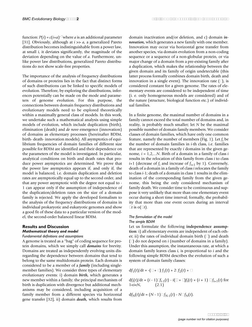
In a finite genome, the maximal number of domains in afamily cannot exceed the total number of domains and, inreality, is probably much smaller; let N be the maximalpossible number of domain family members. We considerclasses of domain families, which have only one commonfeature, namely the number of members (Fig. 1). Let fi bethe number of domain families in i-th class, i.e. familiesthat are represented by exactly i domains in the given ge-nome, i = 1,2,...N. Birth of a domain in a family of class iresults in the relocation of this family from class i to classi+1 (decrease of fi and increase of fi+1 by 1). Conversely,death of a domain in a family of class i relocates the familyto class i-1; death of a domain in class 1 results in the elim-ination of the corresponding family from the given ge-nome, this being the only considered mechanism offamily death. We consider time to be continuous and sup-pose it very unlikely that more than one elementary eventoccur during a short time interval; formally, the probabil-ity that more than one event occurs during an interval∆t is o(∆t).
The formulation of the modelThe simple BDIMLet us formulate the following independence assump-tion: i) all elementary events are independent of each oth-er; ii) the rates of individual domain birth (λ) and death(δ) do not depend on i (number of domains in a family).Under this assumption, the instantaneous rate, at which adomain family leaves class i, is proportional to i and thefollowing simple BDIM describes the evolution of such asystem of domain family classes:
df1(t)/dt = -(λ + δ) f1(t) + 2δf2(t) + ν
dfi(t)/dt = (i - 1)λfi-1(t) - i(λ + δ)fi(t) + (i + 1) δ fi+1(t) for1<i<N, (2.1)
dfN(t)/dt = (N - 1)λ fN-1(t) - Nδ fN(t).
Page 3 of 26(page number not for citation purposes)

BMC Evolutionary Biology 2002, 2 http://www.biomedcentral.com/1471-2148/2/18
Similar models have been considered previously in sever-al different contexts [33 v. 1, ch. 17, 34]. We will see in 3.2that the solution of model (2.1) evolves to equilibrium,with a unique distribution of domain family sizes, fi~(λ/δ)i/i; in particular, if λ = δ, then fi~1/i. Thus, under thesimple BDIM, if the birth rate equals the death rate, theabundance of a domain class is inversely proportional tothe size of the families in this class. When the observa-tions do not fit this particular asymptotic (as observed inseveral studies on distributions of protein family sizes), adifferent, more general model needs to be developed.
The Master BDIMA more general BDIM emerges when the independence as-sumption is abandoned. Instead of constructing specifichypotheses regarding the dependence between the ele-mentary events, let us simply suppose that the domainbirth and death rates for a family of class i do not neces-sarily show proportionality to i. For the general case, wedesignate these rates, respectively, λi and δi; in the specificcase of the simple BDIM (2.1), λi = λi and δi = δi. Then wehave the following master BDIM:
df1(t)/dt = -(λ1 + δ1)f1(t) + δ2f2(t) + ν
dfi(t)/dt = λi-1fi-1(t) - (λi + δi)fi(t) + δi+1fi+1(t) for 1<i<N, (2.2)
dfN(t)/dt = λN-1fN-1(t) - δNfN (t).
Let F(t)= fi(t) be the total number of domain families
at instant t; it follows from (2.2) that
dF(t)/dt = ν - δ1f1(t) (2.3)
The system (2.2) has an equilibrium solution f1,...fN de-fined by the equality dfi(t)/dt = 0 for all i; this solution isdescribed below under Proposition 1. Accordingly, thereexists an equilibrium solution of equation (2.3), whichwe will designate Feq (the total number of domain fami-lies at equilibrium). At equilibrium, ν = δ1f1, i.e. the proc-esses of innovation and death of single domains (moreprecisely, the death of domain families of class 1, i.e. sin-gletons) are balanced.
We can rewrite the model (2.2) in terms of the frequencyof a domain family of class i pi(t) = fi(t)/F(t). Let x(t) =y(t)/Y(t); then
dx/dt = [dy/dt /y - dY/dt /Y] x.
Applying this identity to pi(t) and rewriting equation (2.3)in the form
[dF(t)/dt]/F(t) = ν/F(t) - δ1p1(t) (2.3')
we obtain the following model for frequencies of the do-main family (master BDIM for frequencies), which is equiv-alent to (2.2):
dp1(t)/dt = -(λ1 + δ1)p1(t) + δ2p2(t) + ν/F(t) - (ν/F(t) -δ1p1(t))p1(t), (2.4)
dpi(t)/dt = λi-1pi-1(t) - (λi + δi)pi(t) + δi+1pi+1(t) - (ν/F(t) -δ1p1(t)) pi(t) for 1<i<N,
dpN(t)/dt = λN-1pN-1(t) - δNpN (t) - (ν/F(t) - δ1p1(t))] pN(t).
System (2.4) should be solved together with equation(2.3).
The Master BDIM and Markov processesLet us note that system (2.4) for frequencies is non-linear,so it is not a system of Kolmogorov equations for stateprobabilities of any homogeneous Markov process. Let usfurther suppose that a genome had ample time to arrive atan equilibrium with respect to the total number of do-main families, such that F(t) = Feq. This does not implydpi(t)/dt = 0 or dfi(t)/dt = 0; in other words, the systemmight rearrange the frequencies of individual families, al-though the total number of families remains stable. If F(t)= Feq, the master system (2.4) turns into
Figure 1Domain dynamics and elementary evolutionary events underBDIM.
λ1
δ2
λ2
δ3
λ3
δ4
λi-1
δi
λi
δi+1
λN-1
δN
… …δ1
ν
1f1
2f2
3f3
ifi
NfN
λi
δi
a domain
a domain family
a domain birth in a family moves it one class upper-family birth rate
a domain death in a family moves it one class downper-family death rate
ν innovation adds a single-domain family
i
N
=∑
1
Page 4 of 26(page number not for citation purposes)
BMC Evolutionary Biology 2002, 2 http://www.biomedcentral.com/1471-2148/2/18
d p1(t)/dt = -(λ1 + δ1) p1(t) + δ2p2(t) + ν/Feq (2.5)
d pi(t)/dt = λi-1pi-1(t) - (λi + δi) pi(t) + δi+1pi+1(t) for 1<i<N,
d pN(t)/dt = λN-1pN-1(t) - δNpN (t).
System (2.5) can be rewritten as a matrix equation
dp(t)/dt = p(t)Q,
where p(t) = {p1(t),...pN(t)} and the matrix Q = (qij) is de-fined by equalities
q11 = -(λ1 + δ1) + ν/Feq, q21 = δ2 + ν/Feq, qs1 = ν/Feq for alls > 2;
qi-1,i = λi-1, qi,i = -(λi + δi), qi+1,i = δi+1, qk,i = 0 for all k, |i-k| > 1, i = 2,...N-1,
qN-1,N = λN-1, qN,N = -δN.
It is easy to see that the sum of elements of each row (ex-cept for the first one) of the matrix Q is equal to ν/Feq > 0.Therefore the matrix Q cannot be a matrix of transitionrates for any Markov process (the sum of elements of eachrow of a matrix of transition rates for Markov process withcontinuous time should be non-positive [33 v. 1, ch.17, s.8, 35 v. 2, ch. 3, s. 2]; in other words, there is no Markovprocess with continuous time and state space {1,2,...N}whose state probabilities satisfy system (2.5).
Thus, neither the initial BDIMs (2.1) or (2.2) nor the equi-librium model (2.5) can be described by any Markovprocess with continuous time.
Remark. If, in system (2.5), ν = 0, then this system turnsinto a system of state probabilities for a Markov birth anddeath process with continuous time.
Equilibrium in BDIMsEquilibrium sizes and frequencies of the domain family systemLet us suppose that the genome had ample time to arriveat a complete equilibrium state, in which not only dF(t)/dt = 0, but also dfi(t)/dt = 0 for all i. Thus, the equilibriumsizes of domain families fi satisfy the system
-(λ1 + δ1) f1 + δ2f2 + ν = 0,
λi-1fi-1 - (λi + δi)fi + δi+1fi+1 = 0 for 1<i<N, (3.1)
λN-1fN-1 - δNfN = 0.
It should be emphasized that the master model does notassign a priori the value of Feq; this value has to be comput-ed depending on the model parameters.
The following statement is central for further analysis.
Proposition 1. The master BDIM (2.2) has a unique equilib-rium state (f1,...fN), which is the sole solution of system (3.1):
f1 = ν/δ1
fi = ν λj / δj for all i = 2,...N. (3.2)
The unique equilibrium state (3.2) is globally asymptoticallystable.
In addition (formally assuming λj = 1 for i = 1),
Feq = ν ( λj / δj (3.3)
This proposition ascertains that all evolutionary trajecto-ries of the system (2.2) exponentially (with respect totime) approach the equilibrium state (3.2). The proof isgiven in the Mathematical Appendix.
Remark. Let us denote the ratio of the birth rate to the in-novation rate
G(N) ≡ λifi/ν,
and the ratio of the death rate to the innovation rate
I(N) ≡ δifi/ν.
Then, according to Proposition 1, for any BDIM in equi-librium,
G(N) - I(N) = λj / δj - λj/δj - 1 = -1.
The principal goal of the treatment that follows is theanalysis of the asymptotic behavior of equilibrium fre-quencies and sizes of domain families (f1,...fN) at large N.We will differentiate two cases of asymptotic behavior ac-cording to the following
j
i
=
−
∏1
1
j
i
=∏
1
j
i
=
−
∏1
1
j
i
=
−
∏1
1
j
i
=∏
1
i
N
=
−
∑1
1
i
N
=∑
1
i
N
=
−
∑1
1
j
i
=∏
1 i
N
=
−
∑1
1
j
i
=∏
1
i
N
=∑
1
Page 5 of 26(page number not for citation purposes)
BMC Evolutionary Biology 2002, 2 http://www.biomedcentral.com/1471-2148/2/18
Definition. Let {qi}, {si} be sequences of real numbers;let us denote qi si if lim qi/si = 1 and qi ~ si if lim qi/si = c= const and 0<c<∞. We will also use this notation for finitebut sufficiently long sequences.
Equilibrium frequencies for the simple BDIMLet us apply Proposition 1 to the simple BDIM (2.1) withλi = λi, δi = δi.
Definition. A simple BDIM is balanced if θ = λ/δ = 1, i.e. ifthe rates of individual domain birth and death are equal.
Let us recall that a random discrete variable ξ has the log-arithmic distribution with parameter θ < 1 if
P(ξ = i) = θi/i [-ln(1-θ)]-1, i = 1,2,...
A random variable ξ has the truncated logarithmic distribu-tion with parameter θ if
P (ξ = i) = Cn θi / i, i = 1,2,...n, Cn = 1/ θj/j.
Then, we have
Proposition 2.
1) For any simple BDIM (2.1)
fi = (ν/δ)θi-1/i = (ν/λ)θi/i, (3.4)
Feq = fi = ν/δ θj-1/j, (3.5)
and
pi = (1/Feq)(ν/δ)θi-1/i = (θi/i) / θj/j (3.6)
that is, the equilibrium frequencies have the truncated logarith-mic distribution if θ < 1.
2) If a simple BDIM is balanced, then
Feq = ν/δ 1/j, (3.7)
and for all i = 1,2,...N
pi = ν/δFeq/i = ( 1/j)-1 / i. (3.8)
The proof is given in the Mathematical Appendix.
Thus, a simple BDIM can have equilibrium frequenciesonly of the form pi = Cθi/i, where C = const and θ is the dis-tribution parameter. In particular, the equilibrium fre-quencies for a balanced simple BDIM have the powerdistribution with the degree equal to -1.
Simple methods exist for preliminary graphical estima-tion of the single distribution parameter θ [36 ch. 7, s. 7].We will prove in the following section that, if we observea power asymptotic for empirically observed equilibriumfrequencies, then (assuming that the system can be de-scribed by a BDIM), the rates λi and δi should be asymp-totically equal at large i. If, additionally, the degree of theasymptotic is not equal to -1, then the system dynamicscannot be described by a simple BDIM. In this case, it is nec-essary to consider more general models, such as the Mas-ter BDIM (2.2).
Asymptotic behavior of equilibrium frequencies of a Master BDIM: Main TheoremsLet us consider the master BDIM (2.2); we showed in 3.1that its equilibrium frequencies are the solution of the sys-tem
-(λ1 + δ1)p1 + δ2p2 + ν/Feq = 0, (3.9)
λi-1pi-1 - (λi + δi)pi + δi+1pi+1 = 0 for 1<i<N,
λN-1pN-1 - δNpN = 0.
The following theorem gives all possible types of asymp-totic behavior of the equilibrium frequencies and definesthe connections between these asymptotics depending onmodel parameters. In particular, if there is no informationon the exact form of dependence of the rates of birth anddeath of domains on the size of a domain family, the the-orem can be used to qualitatively describe the dynamics ofthe asymptotic behavior of the equilibrium frequencies.
We will prove that the asymptotic behavior of a solutionof system (3.9) is completely defined by the asymptoticrelation between λi and δi. More precisely, let us define afunction χ (i)= λi-1/δi; we consider only functions of pow-er growth, i.e. χ (i) ~ is at i→∞ for a real s. We will see thatthis is not a serious restriction because the most realisticsituations correspond to the case of s = 0. So, let us sup-pose that, for large i, the following expansion is valid:
≅
i
N
=∑
1
i
N
=∑
1 j
N
=∑
1
j
N
=∑
1
j
N
=∑
1
j
N
=∑
1
Page 6 of 26(page number not for citation purposes)
BMC Evolutionary Biology 2002, 2 http://www.biomedcentral.com/1471-2148/2/18
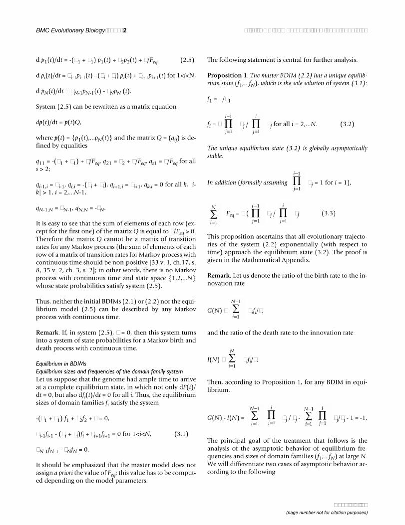
χ (i) ≡ λi-1/δi = is θ (1+a/i + O(1/i2)) (3.10)
where s, a are real numbers and θ > 0. Evidently, if s ≠ 0, χ(i) tends either to 0 (s < 0) or to ∞ (s > 0) with the increaseof i.
Definition. Let us refer to a BDIM (2.2), (3.10) as
i. non-balanced, if s ≠ 0;
ii. first-order balanced, if s = 0 and θ ≠ 1, i.e.
λi-1/δi = θ (1+a/i + O(1/i2)) at large i; (3.11)
iii. second-order balanced, if s = 0, θ = 1 and a ≠ 0, i.e.
λi-1/δi = 1 + a/i + O(1/i2)) for large i; (3.12)
iv. high-order balanced, if s = 0, θ = 1 and a = 0, i.e.
λi-1/δi = 1 + O(1/i2)) for large i.
We will show that the first three coefficients, s, θ and a, ofasymptotic expansion (3.10) for χ (i) = λi-1/δI exactlyspecify all possible asymptotic behaviors of BDIM equilib-rium frequencies.
Theorem 1. The equilibrium frequencies pi of BDIM (2.2)have the following asymptotics
i. if the model is non-balanced, then
pi ~ Γ (i)sθiia, where Γ (i) is the Γ-function;
ii. if the model is first-order balanced, then
pi ~ θiia;
iii. if the model is second-order balanced, then
pi ~ ia;
iv. if the model is high-order balanced, then
pi ~ 1
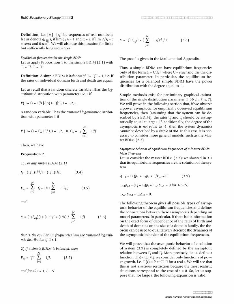
The proof is given in the Mathematical Appendix. Theclassification of BDIM according to the order of balance isillustrated in Fig. 2 and the asymptotics for different typesof BDIMs are shown in Fig. 3.
It follows from this theorem that, if a BDIM is non-bal-anced, then its equilibrium frequencies pi (and equilibri-um family sizes fi) increase or decrease extremely fast(hyper-exponentially) with the increase of i. In contrast, if
a BDIM has a non-zero order of balance, asymptotic be-havior is observed.
Let us recall that a random discrete variable ξ has the Pas-cal (or negative binomial) distribution with parameters (r,q),r > 0, 0 <q < 1, if P(ξ = k) = Γ(r+k)/[Γ(r) Γ(1+k)] (1-q)rqk[36]. We will say that sequence {pi} follows (or as-ymptotically has) a discrete probabilistic distribution {qi}if pi ~ qi for large enough i.
Corollary 1.For a first-order balanced BDIM with θ < 1,
i. if a > -1, the equilibrium frequencies pi follow Pascal distri-bution with parameters (a+1,θ);
Figure 2Different orders of balance in BDIMs.
Figure 3Asymptotics of equilibrium distributions for balanced BDIMsof different orders.
Master BDIMχ(i)=λi-1/δi=isθ(1+a/i+O(1/i2))
s=0s≠0non-balanced
pi~isiθiia
θ≠1first-order balanced
pi~θiia
θ=1
a≠0second-order balanced
pi~ia
a=0high-order balanced
pi~const
1.E-11
1.E-10
1.E-09
1.E-08
1.E-07
1.E-06
1.E-05
1.E-04
1.E-03
1.E-02
1.E-01
1.E+00
1 10 100
-
-
-
-
~i-i0.9ii-2
~0.9ii-2
~i-2
0.01
Page 7 of 26(page number not for citation purposes)
BMC Evolutionary Biology 2002, 2 http://www.biomedcentral.com/1471-2148/2/18
ii. if a = -1, the equilibrium frequencies follow truncated loga-rithmic distribution with parameter θ;
iii. if a = 0, the equilibrium frequencies follow geometric distri-bution with parameter θ.
The following implication of Theorem 1 is of principal in-terest.
Corollary 2. Equilibrium frequencies of a BDIM have a powerasymptotic behavior if and only if the BDIM is second-orderbalanced.
Corollary 3. For high-order balanced BDIM, if λi-1/δi = 1 forall i, the only possible distribution of equilibrium frequencies isuniform, pi = const for all i. Moreover, even if λi-1/δi = 1 +O(1/i2), the equilibrium frequencies asymptotically tend to theuniform distribution.
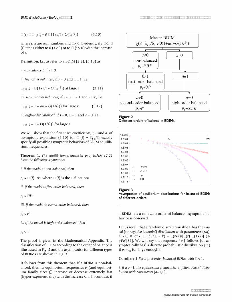
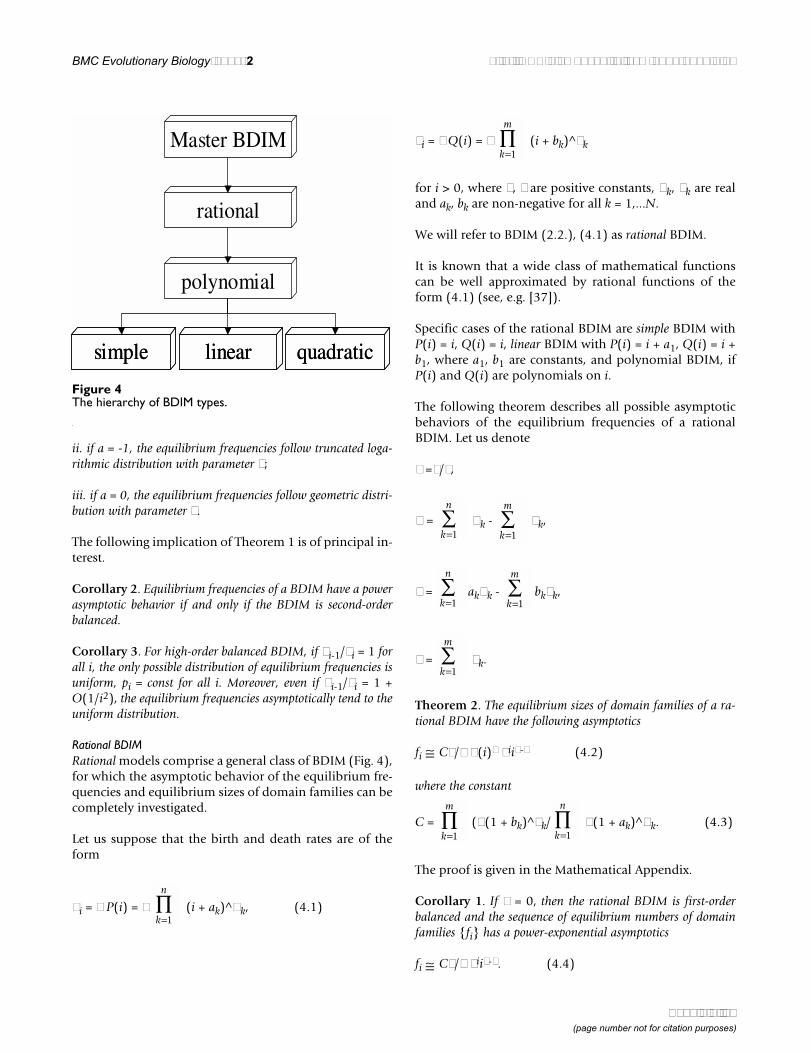
Rational BDIMRational models comprise a general class of BDIM (Fig. 4),for which the asymptotic behavior of the equilibrium fre-quencies and equilibrium sizes of domain families can becompletely investigated.
Let us suppose that the birth and death rates are of theform
λi = λ P(i) = λ (i + ak)^αk, (4.1)
δi = δ Q(i) = δ (i + bk)^βk
for i > 0, where λ, δ are positive constants, αk, βk are realand ak, bk are non-negative for all k = 1,...N.
We will refer to BDIM (2.2.), (4.1) as rational BDIM.
It is known that a wide class of mathematical functionscan be well approximated by rational functions of theform (4.1) (see, e.g. [37]).
Specific cases of the rational BDIM are simple BDIM withP(i) = i, Q(i) = i, linear BDIM with P(i) = i + a1, Q(i) = i +b1, where a1, b1 are constants, and polynomial BDIM, ifP(i) and Q(i) are polynomials on i.
The following theorem describes all possible asymptoticbehaviors of the equilibrium frequencies of a rationalBDIM. Let us denote
θ =λ/δ,
η = αk - βk,
ρ = akαk - bkβk,
β = βk.
Theorem 2. The equilibrium sizes of domain families of a ra-tional BDIM have the following asymptotics
fi Cν/λ Γ(i)η θiiρ-β (4.2)
where the constant
C = (Γ(1 + bk)^βk/ Γ(1 + ak)^αk. (4.3)
The proof is given in the Mathematical Appendix.
Corollary 1. If η = 0, then the rational BDIM is first-orderbalanced and the sequence of equilibrium numbers of domainfamilies {fi} has a power-exponential asymptotics
fi Cν/λ θiiρ-β. (4.4)
Figure 4The hierarchy of BDIM types.
simple linear quadraticsimple linear quadratic
polynomial
rational
Master BDIM
k
n
=∏
1
k
m
=∏
1
k
n
=∑
1 k
m
=∑
1
k
n
=∑
1 k
m
=∑
1
k
m
=∑
1
≅
k
m
=∏
1 k
n
=∏
1
≅
Page 8 of 26(page number not for citation purposes)
BMC Evolutionary Biology 2002, 2 http://www.biomedcentral.com/1471-2148/2/18
In particular, if ρ - β > -1, the equilibrium frequencies pi followthe Pascal distribution with parameters (ρ - β + 1, θ);
if ρ - β = -1, then frequencies pi follow the truncated logarith-mic distribution;
if ρ - β = 0, then frequencies pi follow the geometric distribu-tion.
Corollary 2. The equilibrium sizes of domain families fi andequilibrium frequencies pi for a rational BMID have the powerasymptotics if and only if η = 0 and λ = δ, i.e. the BDIM is sec-ond-order balanced, in which case
fi Cν/λ iρ-β. (4.5)
Formula (4.4) gives the asymptotics for the equilibriumsizes of domain families fi and, accordingly, for the totalnumber of families Feq. The exact expressions for thesequantities are given in the proofs of Theorem 2 and Lem-ma (see Mathematical Appendix).
Proposition 3.
i. The equilibrium sizes of domain families fi of a balanced(first or higher order) rational BDIM are
fi = Cν/δθi-1 [(Γ(i + ak))^αk]/ [(Γ(i + 1 +
bk))^βk] for all i = 1,2,...
where
C = [(Γ(1 + bk))^βk]/ (Γ(1 + ak)^αk].
ii. The total number of domain families at equilibrium is
Feq = Cν/δ( θj-1 (Γ(j + ak))^αk/ (Γ(j + 1 +
bk))^βk).
For the rational, second-order balanced BDIM, the ratio ofthe birth rate to the innovation rate is
G(N) = θi [Γ(i + 1 + ak)/Γ(1 + ak)]^αk / [Γ(i +
1 + bk) / Γ(1 + bk)]^βk.
The asymptotic formulas for equilibrium frequencies ofrational BDIM could be considered as particular cases ofthe corresponding formulas of general theorem 1. Propo-sition 3 allows one to calculate the constants in the corre-sponding asymptotic formulas for the sizes of domainfamilies for a rational BDIM. If only equilibrium frequen-cies are analyzed, the values of these constants become ir-relevant because they contract. However, if the actualvalues of fi and Feq are of interest, the values of the con-stants are required.
Properties of the main types of rational BDIMSimple BDIMAs shown above, a simple BDIM can have equilibrium fre-quencies only of the form pi = Cθi/i, C = const;in particular,if the distribution parameter θ < 1, we get the (truncated)logarithmic distribution. Logarithmic distributions areseen in many biological contexts, e.g., the distribution ofspecies by the number of individuals in populations or,what is more relevant, the distribution of protein folds bythe number of families per fold [38]. Thus, a simple BDIMcould be potentially used for modeling the dynamics ofbiological systems with a logarithmic distribution of equi-librium densities. We examine this possibility in greaterdetail starting with the case λ = δ (second-order balancedsimple BDIM).
We can extract from Proposition 2 some additional infor-mation, which could be helpful for estimating the modelparameters. It is known that
1/i = lnN + CE + O (1/N), where CE is the Euler con-
stant, CE = 0.5772157...
More precisely, the approximation
1/i = lnN + CE + N-1/2 - N-2/12 has an error less then
10-6 for N > 10. Thus, from (3.7), we obtain an interestingformula
Feq (ν/δ) [lnN + CE] (5.1)
This means that, in the equilibrium state of the system,the total number of domain families grows only slowly(~ln N) with the increase of the maximal number (N) ofdomains in a family (which is equal to the maximal pos-sible number of domain family size classes).
Furthermore, according to equation (2.3), in the equilib-rium state of a simple BDIM ν/δ = f1, so we have
≅
k
n
=∏
1 k
m
=∏
1
k
m
=∏
1 k
n
=∏
1
j
N
=∑
1 k
n
=∏
1 k
m
=∏
1
i
N
=
−
∑1
1
k
m
=∏
1
i
N
=∑
1
i
N
=∑
1
≅
Page 9 of 26(page number not for citation purposes)
BMC Evolutionary Biology 2002, 2 http://www.biomedcentral.com/1471-2148/2/18
Feq / f1 lnN + CE (5.2)
Formula (5.1) can be used for estimating the model pa-rameters on the basis of empirical data.
In the more general case λ ≠ δ, we can also obtain an esti-mate of the rate of innovation ν. If λ < δ (θ < 1), then theseries in the right part of (3.5) quickly converges,
θi-1/i → -ln(1-θ)/θ,
so -ln(1-θ)/θ is a good approximation for the sum
θi-1/i for large N. Then
Feq = (ν/δ) θi-1/i = (ν/λ) θi/i ν/λ (-ln(1-θ)),
and
ν/δ = Feq θ/(-ln(1-θ)). (5.3)
Taking into account that ν/δ = f1 (2.3), we have a relation
Feq/f1 -ln(1-θ)/θ, (5.4)
which allows the parameter θ to be estimated on the basisof empirical data.
If N can be estimated independently and is not very large,we can use more exact relations:
θi/i -ln(1-θ) + Ei(-N(1-θ)) - N-1/2 + N-2/12.
where the function .
Further, if (1-θ)N is small (i.e., θ is very close to 1), thenthe approximation
θi/i CE - N(1-θ)
has an error less then [N(1-θ)]2/4 and, in this case,
Feq/f1 (CE - N(1 - θ))/θ. (5.5)
If (1 - θ)N is large, then the following inequalities provide
simple bounds for Feq/f1 = θi-1/i:
-(ln(1-θ)/θ-θN/[(N+1)(1-θ)] < θi-1/i < -ln(1-θ)/θ-
θN[1/(N+1)-θ/(N+2)]. (5.6)
For the simple BDIM, the ratio of the rate of duplicationsto the innovation rate is
G(N) = λifi/ν = θi = θ(1-θN-1)/(1-θ),
so G(N) → ∞ if θ > 1 and G(N) → 1/(1-θ) if θ < 1 at N→∞.
If the simple BDIM is the 2nd order balanced, θ = 1, thenG(N) = N - 1.
Thus, for the simple, second-order balanced BDIM, thenumber of duplications per time unit is N-1 times greaterthan the number of innovations.
The total number of domains in the equilibrium state forthe simple BDIM is
M(N) = ifi = ν/λθ(1-θN)/(1-θ).
If a simple BDIM is second-order balanced, then G(N) =ν/λ N.
Linear BDIMWe saw that the assumption of independence of birth anddeath rates of individual domains on each other and onthe size of domain families is incompatible with any pow-er distribution of the equilibrium frequencies with the de-gree not equal to -1. The simplest case of a BDIM, whichcan have, depending on the parameters, three types of as-ymptotic behavior described by Theorem 1 (excluding thefirst one, hyper-exponential, which corresponds to a non-balanced BDIM; all linear BDIMs are balanced) and, inparticular, any power asymptotics, is a model with linearbirth and death rates of the form:
λi = λ (i + a), δi = δ (i + b), where a and b are constants. (5.7)
The parameters a and b account, in the simplest possibleform, for the deviation of the domain birth and death
≅
i
N
=∑
1
i
N
=∑
1
i
N
=∑
1 i
N
=∑
1≅
≅
i
N
=∑
1≅
Ei u e xdxxu
( ) =−∞∫ /
i
N
=∑
1≅
≅
i
N
=∑
1
i
N
=∑
1
i
N
=
−
∑1
1
i
N
=
−
∑1
1
i
N
=∑
1
Page 10 of 26(page number not for citation purposes)
BMC Evolutionary Biology 2002, 2 http://www.biomedcentral.com/1471-2148/2/18
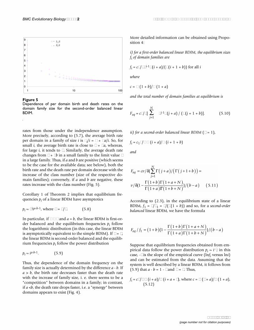
rates from those under the independence assumption.More precisely, according to (5.7), the average birth rateper domain in a family of size i is λi/i = λ + λa/i. So, forsmall i, the average birth rate is close to λ + λa, whereas,for large i, it tends to λ. Similarly, the average death ratechanges from δ + δb in a small family to the limit value δin a large family. Thus, if a and b are positive (which seemsto be the case for the available data; see below), both thebirth rate and the death rate per domain decrease with theincrease of the class number (size of the respective do-main families); conversely, if a and b are negative, theserates increase with the class number (Fig. 5).
Corollary 1 of Theorem 2 implies that equilibrium fre-quencies pi of a linear BDIM have asymptotics
pi ~ θiia-b-1, where θ = λ/δ. (5.8)
In particular, if λ ≠ δ and a = b, the linear BDIM is first-or-der balanced and the equilibrium frequencies pi followthe logarithmic distribution (in this case, the linear BDIMis asymptotically equivalent to the simple BDIM). If λ = δ,the linear BDIM is second-order balanced and the equilib-rium frequencies pi follow the power distribution
pi ~ ia-b-1. (5.9)
Thus, the dependence of the domain frequency on thefamily size is actually determined by the difference a - b. Ifa > b, the birth rate decreases faster than the death ratewith the increase of family size, i. e. there seems to be a"competition" between domains in a family; in contrast,if a <b, the death rate drops faster, i.e. a "synergy" betweendomains appears to exist (Fig. 4).
More detailed information can be obtained using Propo-sition 4:
i) for a first-order balanced linear BDIM, the equilibrium sizesfi of domain families are
fi = cν/δθi-1Γ(i + a)/(Γ(i + 1 + b)) for all i
where
c = Γ (1 + b)/Γ (1 + a)
and the total number of domain families at equilibrium is
Feq = cν/δ[ θj-1Γ(j + a) / (Γ(j + 1 + b)]. (5.10)
ii) for a second-order balanced linear BDIM (θ = 1),
fi = c1ν/δ Γ (i + a)/Γ (i + 1 + b)
and
According to (2.3), in the equilibrium state of a linearBDIM, f1 = ν/δ1 = ν/(δ(1 + b)) and so, for a second-orderbalanced linear BDIM, we have the formula
Suppose that equilibrium frequencies obtained from em-pirical data follow the power distribution pi ~ i-γ; in thiscase, -γ is the slope of the empirical curve (lnfi versus lni)and can be estimated from the data. Assuming that thesystem is well described by a linear BDIM, it follows from(5.9) that a - b = 1 - γ and λ = δ. Thus,
fi = cν/δ Γ (i + a)/Γ (i + a + γ), where c = Γ (γ + a)/Γ (1 + a), (5.12)
Figure 5Dependence of per domain birth and death rates on thedomain family size for the second-order balanced linearBDIM.
0
1
2
3
4
5
6
7
8
9
1 10 100
-
-
λi /iδi /i
j
N
=∑
1
F cv j a j b
vb a N
a
eqj
N= +( ) + +( )( ) =
−+( ) + +( )+( )
=∑/ ( /
/ (
δ
δ
Γ Γ
Γ ΓΓ
1
11 1
1
1
ΓΓ 15 11
+ +( ) −( ) ( )b N
b a)/ .
F f bb a N
a b Nb aeq / ( )/1 1 1
1 1
1 1= +( ) −
+( ) + +( )+( ) + +( ) −( )Γ Γ
Γ Γ
Page 11 of 26(page number not for citation purposes)
BMC Evolutionary Biology 2002, 2 http://www.biomedcentral.com/1471-2148/2/18
and
where a is the single free parameter.
For the linear second-order balanced BDIM, the ratio ofthe birth rate to the innovation rate is
if 1 + a - b ≠ 0. As
if 1 + a - b < 0 and G(N)→∞ if 1 + a - b > 0 at N→∞.
The case 1 + a - b = 0 (slope of the asymptote in doublelogarithmic coordinates equal to a - b - 1 = -2) is a criticalone.
In this case,
G(N) = Γ(1 + b) / Γ(b) Γ (i + b) / (Γ (i + 1 + b) =
b1/(i + b) = b [PolyGamma(0, b+N) - PolyGam-
ma(0, b+1)].
Accordingly, G(N)→∞ at N→∞.
The total number of domains in the equilibrium state fora second-order balanced linear BDIM is
If the slope of the asymptote γ = -1, the linear second-or-dered BDIM shows the same asymptotic behavior as asimple BDIM (2.1), but behaves differently at small i. If γ≠ -1, the system cannot be described by a simple BDIMeven asymptotically, but can be described by a linearBDIM. As indicated above, in this case, the average per-do-main birth and death rates depend on the size of the do-main family and the difference a-b characterizes thisdependence.
Quadratic BDIMThe linear BDIM takes into account the dependence of av-erage birth and death rates of individual domains on thesize of domain family, but does not imply a specific formof interaction between domains. Let us consider the sim-plest, pairwise interaction, which leads to λi ~ i2 and/or δi~ i2, i.e. one or both rates are polynomials on i of the sec-ond degree. If these degrees are different (i.e., λi ~ i and δi~ i2), then the corresponding BDIM is non-balanced andequilibrium frequencies have hyper-exponential asymp-totics. Thus, let
λi = λ (i2 + r1i + r2), δi = δ (i2 + q1i + q2), (5.13)
where rk, qk, k = 1,2 are constants (such that λi, δi are pos-itive for all i) or
λi = λ (i + a1)(i + a2),
δi = δ (i + b1)(i + b2)
Then, r1 = a1 + a2, q1 = b1 + b2, and
χ (i) = λi-1/δi = θ (1 + (r1-q1-2)/i + O(1/i2)),
where θ = λ/δ.
According to theorem 3 and Proposition 3, the quadraticBDIM with rates (5.13) has equilibrium sizes of domainfamilies
F cv j a j a
va N a
a N
eqj
N= +( ) + +( ) =
−+ +( ) +( )+ +( )
=∑/ /
/ (
δ γ
δγ
γ
Γ Γ
Γ ΓΓ Γ
1
11
111
+( ) −( )a
)/ γ
F f a ka N a
a N aeq / ( )/1 11
11= +( ) −
+ +( ) +( )+ +( ) +( ) −( )Γ Γ
Γ Γγ
γγ
G N f v b a i a i a i bi ii
N
i
N
( ) = = +( ) +( ) +( ) +( ) + +( )=
−
=
−
∑ λ / / /(1
1
1
1 1 1Γ Γ Γ Γ11
1
11 1 1 1
1 1
1
∑
∑
=
+( ) +( ) + +( ) + +( ) =
+ +( ) +( )=
−Γ Γ Γ Γ
Γ Γ
b a i a i b
a N bi
N/ /(
++ −( ) +( ) +( ) ++
− −a b b N a
a
b aΓ Γ 11
1
Γ ΓΓ Γ
ΓΓ
1 1
1 1
1
1 11+ +( ) +( )
+ −( ) +( ) +( ) ≅+( )
+ −( ) +( )+ −a N b
a b b N a
b
a b aN a bb
G Na
b a
,
( ) →+
− −1
1
i
N
=
−
∑1
1
i
N
=
−
∑1
1
M N if
v i b a i a i b
va
ii
N
i
N
( ) = =
+( ) +( ) +( ) + +( ) =
=
=
∑
∑1
1
1 1 1/ / /(
/ [
δ
δ
Γ Γ Γ Γ
aa b
a
b a
b
b N
N a
a b a
N a
−+
+− −
++( )
+ +( )+ +( )
+ −( ) −( ) −+ +(1
1
1
1
2
1 1
1ΓΓ
ΓΓ
Γ(
))−( ) ( )a b aΓ
)].
Page 12 of 26(page number not for citation purposes)

BMC Evolutionary Biology 2002, 2 http://www.biomedcentral.com/1471-2148/2/18
fi = c2 ν/δ θi-1 Γ (i + a1) Γ (i + a2) / (Γ (i + 1 + b1) (Γ (i + 1+ b2)) c2ν/δ θi-1iρ-2 (5.14)
where ρ = r1 - q1 and the constant c2 = [(Γ (1+b1) Γ (1+b2)]/ [Γ (1+a1) Γ (1+a2)], and the total number of domainfamilies at equilibrium
Feq = c2ν/δ ( θj-1 Γ(j+a1) Γ(j+a2) / (Γ(j+1+b1)
(Γ(j+1+b2)). (5.15)
Note that the asymptotic behavior of frequencies pi doesnot depend on free coefficients r2, q2 in (5.13), but onlyon θ and r1-q1 (as follows from (5.14)), although the val-ues of fi are proportional to the constant c2, which coulddepend on the free coefficients r2, q2. Let us consider thecase r2 = q2 = 0 in more detail.
If only square terms are present in the expressions for thebirth and death rates, λi = λi2, δi = δi2, then ak = bk = 0, k =
1,2 and so c2 = 1, fi = ν/δ θi-1/i2 and Feq = ν/δ θj-1/j2.
So at N→∞
Feq ν/δ θj-1 / j2 = ν/λ Polylog(2,θ) (5.16)
where Polylog is a special function, Polylog(k,x) = xj/
jk.
According to (3.2), f1 = ν/δ1; for this particular case ofquadratic BDIM, f1 = ν/δ and
Feq/f1 Polylog(2,θ). (5.17)
Formula (5.17) allows estimating parameter θ fromempirical data if N is large enough.
More precisely, Feq = ν/λ θj/j2 = ν/λ (Polylog(2,θ)-
θ1+N LerchPhi(θ,2,1+N)), where LerchPhi is a specialfunction (these and other special functions used belowcan be computed using program packages Mathematikaor Maple).
If, additionally, θ = 1 (the BDIM is second-order bal-anced), then
fi = (ν/δ)/i2 = f1/i2 (5.18)
and, at large N
Feq ν/δ π2/6 1.645 ν/δ = 1.645f1. (5.19)
From formulas (5.8), (5.15), we can extract some addi-tional information, which could be helpful for estimatingthe model parameters at relatively small N. Let us recalldefinitions of some special functions.
The digamma function φ(z) is logarithmic derivative ofΓ(z), φ(z) = Γ'(z)/Γ(z).
The function PolyGamma(n,z) is nth derivative of φ(z),PolyGamma(n,z) = dnφ(z)/dzn, such that φ(z)= PolyGam-ma(0,z).
It is known that
1/i2 = π2/6-PolyGamma(1,1+N),
Thus we have
Feq = ν/δ 1/j2 = ν/δ [π2/6-PolyGamma(1,1+N)]
(5.20)
Feq/f1 = π2/6-PolyGamma(1,1+N),
which can be used for estimating unknown parameters ofthe model.
The values of PolyGamma(1,x) are tabulated and can becomputed using standard program packages; for a roughpreliminary estimate, PolyGamma(1,x) = 1/x+1/2x2+O(1/x4).
If linear terms are also present in the quadratic BDIM, λi =λ (i2+a1i), δi = δ (i2+b1i), then
fi = c2ν/δ θi-1/i Γ (i+a1)/Γ (i+1+b1)
where c2 = Γ (1+b1)/Γ (1+a1); Feq = Σfi can be computedusing special functions. In particular, if the BDIM is sec-ond-order balanced, θ = 1, then
≅
j
N
=∑
1
j
N
=∑
1
≅j
∑
j=
∞
∑1
≅
j
N
=∑
1
≅ ≅
i
N
=∑
1
j
N
=∑
1
Page 13 of 26(page number not for citation purposes)
BMC Evolutionary Biology 2002, 2 http://www.biomedcentral.com/1471-2148/2/18
fi = c2ν/δ Γ (i+a1) / (i Γ (i+1+b1)).
For this variant of the model, f1 = ν/δ1 = ν/(δ(1+b1)), andso
Polynomial BDIMsThe quadratic models take into account the dependenceof birth and death rates of individual domains on the sim-plest, pairwise interactions. If interactions of higher ordersare postulated, λi ~ Pn(i) and/or δi ~ Qm(i), where Pn(i),Qm(i) are polynomials on i of the n-th and m-th degrees.Again, if the degrees n and m are different, then the BDIMis non-balanced and equilibrium frequencies have hyper-exponential asymptotics. Thus, let n = m,
λi = λR (i) = λ rkim-k, δi = δQ(i) = δ qkim-k
(5.21)
where rk, qk are constants and r0 = q0 = 1. We suppose, ofcourse, that R(i), Q(i) are positive for all integer i. Notethat, in this case, χ (i) ≡ λi-1/δi = θ (1+(r1 - q1 - m)/i+O(1/i2)), where θ = λ/δ. We will suppose that θ ≤ 1.
According to Theorem 3, the polynomial BDIM with rates(5.21) has equilibrium sizes of domain families with pow-er-exponential asymptotics
fi ~ θiiρ-m (5.22)
where ρ = r1 - q1.
In particular, if ρ - m > -1, the equilibrium frequencies pifollow the Pascal distribution with parameters (ρ - m + 1,θ);
if ρ - m = -1, the equilibrium frequencies pi follow the(truncated) logarithmic distribution;
if ρ - m = 0, the equilibrium frequencies pi follow the geo-metric distribution;
if λ = δ, the polynomial BDIM is second-order balancedand the equilibrium frequencies pi follow the power dis-tribution
pi ~ iρ-m. (5.23)
Note that the degree of the power distribution (5.23) de-pends only on m, the common degree of the polynomials(5.21), and on ρ, the difference between the coefficients r1and q1, and does not depend on other coefficients. In par-
ticular, if r1 = q1, then pi ~ i-m. This relation could be inter-preted as follows: if the first two coefficients ofpolynomial rates λi and δi are equal, then the degree of thepower distribution (5.19) is equal to the "order of interac-tions" of domains.
Formula (5.22) can be refined. Let R(i) = (i+ak), Q(i)
= (i+bk).
Then (see Proposition 3) the equilibrium numbers of do-main families fi of the polynomial BDIM (5.18) are
fi = Cν/δθi-1 [Γ(i+ak)/Γ(i+1+bk)]
where C = [Γ(1+bk)/Γ(1+ak)], and the equilibrium
total number of domain families
Feq = Cν/δ θj-1 [Γ(j+ak)/Γ(j+1+bk)].
For the polynomial model f1 = ν/δ1 = ν/(δ qk), so
Feq/f1 = C θj-1 (Γ(j+ak)/Γ(j+1+bk))/ qk.
This formula can be used for estimating the model param-eters.
For the polynomial second-order balanced BDIM, the ra-tio of the death rate to the innovation rate is
G(N) = λifi/ν = ( Γ(1+bk)/Γ(1+ak))
Γ(i+1+ak)/Γ(i+1+bk) =
[Γ(i+1+ak)/Γ(1+ak)]/[Γ(i+1+bk)/Γ(1+bk)].
f fb i a
i a i bi =+( ) +( )
+( ) + +( )11 1
1 1
2
1 1
Γ ΓΓ Γ
.
k
m
=∑
0 k
m
=∑
0
k
m
=∏
1
k
m
=∏
1
k
m
=∏
1
k
m
=∏
1
j
N
=∑
1 k
m
=∏
1
k
m
=∑
0
j
N
=∑
1 k
m
=∏
1 k
m
=∑
0
i
N
=
−
∑1
1
k
m
=∏
1
i
N
=
−
∑1
1
k
m
=∏
1
i
N
=
−
∑1
1
k
m
=∏
1
Page 14 of 26(page number not for citation purposes)
BMC Evolutionary Biology 2002, 2 http://www.biomedcentral.com/1471-2148/2/18
Approximation of the observed domain family size distributions in prokaryotic and eukaryotic genomes with different BDIMsHaving developed the mathematical theory of BDIMs, wesought to determine which of these models, if any, ade-quately described the empirical data on domain familysize distribution. To identify the domain sets of domainsencoded in each of the genomes, the CDD library of posi-tion-specific scoring matrices (PSSMs), which includes thedomains from the Pfam and SMART databases, was usedin RPS-BLAST searches [12] against the protein sequencesfrom a set of completely sequenced eukaryotic andprokaryotic genomes [http://www.ncbi.nlm.nih.gov/ent-rez/query.fcgi?db=Genome]. The CDD domain library ispartially redundant, so when the results obtained from in-dividual PSSMs showed significant overlap (more than50% of hits overlapped for more than 50% of theirlength), the corresponding domains were examined case-by-case for redundancy. PSSMs representing structurallysimilar domains and producing overlapping lists of hitswere joined into "synonymy clusters".
The results of RPS-BLAST searches against the sets of pro-tein sequences from individual genomes were interpretedas follows: non-overlapping hits to the same protein weretreated independently; among overlapping hits, only thestrongest one (lowest E-value) was recorded; all hits froma synonymy cluster were assigned to one representativedomain family. The number of hits that a domain familyhad in a genome, with the cut-off of E = 0.001, was record-ed as the number of domains of the given family encodedin the given genome. The CDD domain library certainly
does not include all existing domains. In practice, do-mains from this collection were detected in >50% in eachof the analyzed species, with the only exception of hu-man, for which the analyzed protein set is likely to con-tain a substantial fraction of false predictions (Table 1).
To enable statistical analysis using the χ2-method for theentire range of the data, including the sparsely distributedclasses corresponding to large families, the data needed tobe combined. For each genome, the observed domainfamily frequencies were grouped into bins, each contain-ing at least 10 families; typically, bins corresponding tofamilies with small number of members included a singlesize class (e.g. all single-member families, two-memberfamilies etc), whereas bins corresponding to large familiesmay span hundreds of size classes, most of them empty.Theoretical distribution values for a bin combining ob-served data from m-th to n-th class were computed as
, where f'i is the predicted number of families in
the i-th class and depends on the model parameters. Sincethe model displays only a weak dependence on the maxi-mum number of domains in a family (N), instead of in-
cluding N as a model parameter, the sum (where
imax is the number of domains in the most abundant ofthe detected families), was normalized to equal the totalnumber of families detected in the given genome (a re-
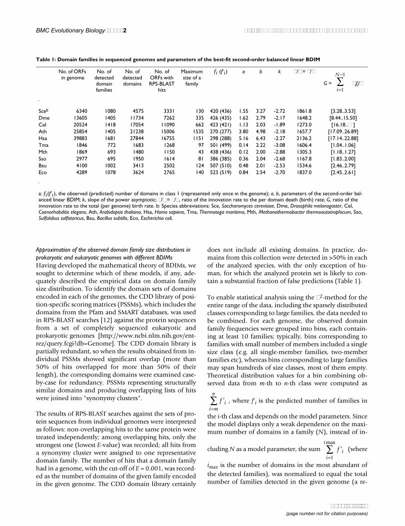
Table 1: Domain families in sequenced genomes and parameters of the best-fit second-order balanced linear BDIM
No. of ORFs in genome
No. of detected domain families
No. of detected domains
No. of ORFs with RPS-BLAST
hits
Maximum size of a family
f1 (f'1) a b k ν/δ = ν/λ
G = λifi/ν
Sceb 6340 1080 4575 3331 130 420 (436) 1.55 3.27 -2.72 1861.8 [3.28..3.53]Dme 13605 1405 11734 7262 335 426 (435) 1.62 2.79 -2.17 1648.2 [8.44..15.50]Cel 20524 1418 17054 11090 662 423 (421) 1.13 2.03 -1.89 1273.0 [16.18..∞ ]Ath 25854 1405 21238 15006 1535 270 (277) 3.80 4.98 -2.18 1657.7 [17.09..26.89]Hsa 39883 1681 27844 16755 1151 298 (288) 5.16 6.43 -2.27 2136.2 [17.14..22.88]Tma 1846 772 1683 1268 97 501 (499) 0.14 2.22 -3.08 1606.4 [1.04..1.06]Mth 1869 693 1480 1150 43 438 (436) 0.12 2.00 -2.88 1305.3 [1.18..1.27]Sso 2977 695 1950 1614 81 386 (385) 0.36 2.04 -2.68 1167.8 [1.83..2.00]Bsu 4100 1002 3413 2502 124 507 (510) 0.48 2.01 -2.53 1534.6 [2.46..2.79]Eco 4289 1078 3624 2765 140 523 (519) 0.84 2.54 -2.70 1837.0 [2.45..2.61]
a: f1(f'1), the observed (predicted) number of domains in class 1 (represented only once in the genome); a, b, parameters of the second-order bal-anced linear BDIM; k, slope of the power asymptotic; ν/δ = ν/λ, ratio of the innovation rate to the per domain death (birth) rate; G, ratio of the innovation rate to the total (per genome) birth rate. b: Species abbreviations: Sce, Saccharomyces cerevisiae, Dme, Drosophila melanogaster, Cel, Caenorhabditis elegans, Ath, Arabidopsis thaliana, Hsa, Homo sapiens, Tma, Thermotoga maritima, Mth, Methanothermobacter thermoautotrophicum, Sso, Sulfolobus solfataricus, Bsu, Bacillus subtilis, Eco, Escherichia coli.
i
N
=
−
∑1
1
f ii m
n’
=∑
f ii
i’
max
=∑
1
Page 15 of 26(page number not for citation purposes)
BMC Evolutionary Biology 2002, 2 http://www.biomedcentral.com/1471-2148/2/18
quirement for the χ2 analysis). χ2 values were computedto measure the quality of fit between the observed and thetheoretical distributions. The distribution parameters (θfor the simple BDIM, a and b for the second-order bal-anced linear BDIM) were adjusted to minimize the χ2 val-ue.
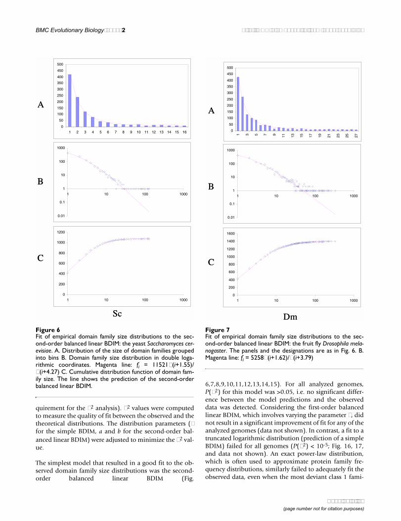
The simplest model that resulted in a good fit to the ob-served domain family size distributions was the second-order balanced linear BDIM (Fig.
6,7,8,9,10,11,12,13,14,15). For all analyzed genomes,P(χ2) for this model was >0.05, i.e. no significant differ-ence between the model predictions and the observeddata was detected. Considering the first-order balancedlinear BDIM, which involves varying the parameter θ, didnot result in a significant improvement of fit for any of theanalyzed genomes (data not shown). In contrast, a fit to atruncated logarithmic distribution (prediction of a simpleBDIM) failed for all genomes (P(χ2) < 10-5; Fig. 16, 17,and data not shown). An exact power-law distribution,which is often used to approximate protein family fre-quency distributions, similarly failed to adequately fit theobserved data, even when the most deviant class 1 fami-
Figure 6Fit of empirical domain family size distributions to the sec-ond-order balanced linear BDIM: the yeast Saccharomyces cer-evisiae. A. Distribution of the size of domain families groupedinto bins B. Domain family size distribution in double loga-rithmic coordinates. Magenta line: fi = 11521Γ(i+1.55)/Γ(i+4.27) C. Cumulative distribution function of domain fam-ily size. The line shows the prediction of the second-orderbalanced linear BDIM.
0
50
100
150
200
250
300
350
400
450
500
1 2 3 4 5 6 7 8 9 10 11 12 13 14 15 16
0.01
0.1
1
10
100
1000
1 10 100 1000
0
200
400
600
800
1000
1200
1 10 100 1000
A
B
C
Sc
A
B
C
Sc
Figure 7Fit of empirical domain family size distributions to the sec-ond-order balanced linear BDIM: the fruit fly Drosophila mela-nogaster. The panels and the designations are as in Fig. 6. B.Magenta line: fi = 5258Γ(i+1.62)/Γ(i+3.79)
0
50
100
150
200
250
300
350
400
450
500
1 3 5 7 9 11 13 15 17 19 21 23 25 27
0.01
0.1
1
10
100
1000
1 10 100 1000
0
200
400
600
800
1000
1200
1400
1600
1 10 100 1000
A
B
C
Dm
A
B
C
Dm
Page 16 of 26(page number not for citation purposes)

BMC Evolutionary Biology 2002, 2 http://www.biomedcentral.com/1471-2148/2/18
lies were excluded (P(χ2) = 0.0013 for T. maritima; P(χ2)< 10-5 for the rest of the genomes; Fig. 16, 17 and data notshown). Notably, second-order balanced linear BDIM re-sults in a correct prediction of the number of very largefamilies, whereas simple BDIM systematically underesti-mates the number of families in the highest bins. Con-versely, the power-law fit underestimates the slope of thebest-fit line (in double logarithmic coordinates) com-pared to the asymptote of the linear BDIM prediction and,accordingly, significantly overestimates the number offamilies in the highest bins (Fig. 16, 17). These results arecompatible with the recent observation that the domain
family size distributions are better described by the gener-alized Pareto distribution than by power laws [31].
Fitting the observed domain family size distribution withthe second-order balanced linear BDIM resulted in posi-tive values of the parameters a and b, with a <b, for all an-alyzed genomes (Table 1). Accordingly, domain familysize distributions in all cases asymptotically tend to thepower law with the power k < -1 and, for all species withthe exception of C. elegans, k < -2 (Table 1 and Fig. 8). Asdiscussed above, this seems to indicate the existence of"synergy" between domains in a family whereby the like-lihood of survival is greater for a domain that belongs to
Figure 8Fit of empirical domain family size distributions to the sec-ond-order balanced linear BDIM: the nematode wormCaenorhabditis elegans. The panels and the designations are asin Fig. 6. B. Magenta line: fi = 2453Γ(i+1.13)/Γ(i+3.03)
0
50
100
150
200
250
300
350
400
4501 3 5 7 9 11 13 15 17 19 21 23 25 27 29 31
0.01
0.1
1
10
100
1000
1 10 100 1000
0
200
400
600
800
1000
1200
1400
1600
1 10 100 1000
A
B
C
Ce
A
B
C
CeFigure 9Fit of empirical domain family size distributions to the sec-ond-order balanced linear BDIM: the thale cress Arabidopsisthaliana. The panels and the designations are as in Fig. 6. B.Magenta line: fi = 10750Γ(i+3.80)/Γ(i+5.98)
0
50
100
150
200
250
300
1 3 5 7 9 11 13 15 17 19 21 23 25 27 29 31 33 35
0.001
0.01
0.1
1
10
100
1000
1 10 100 1000 10000
0
200
400
600
800
1000
1200
1400
1600
1 10 100 1000 10000
A
B
C
At
A
B
C
At
Page 17 of 26(page number not for citation purposes)
BMC Evolutionary Biology 2002, 2 http://www.biomedcentral.com/1471-2148/2/18
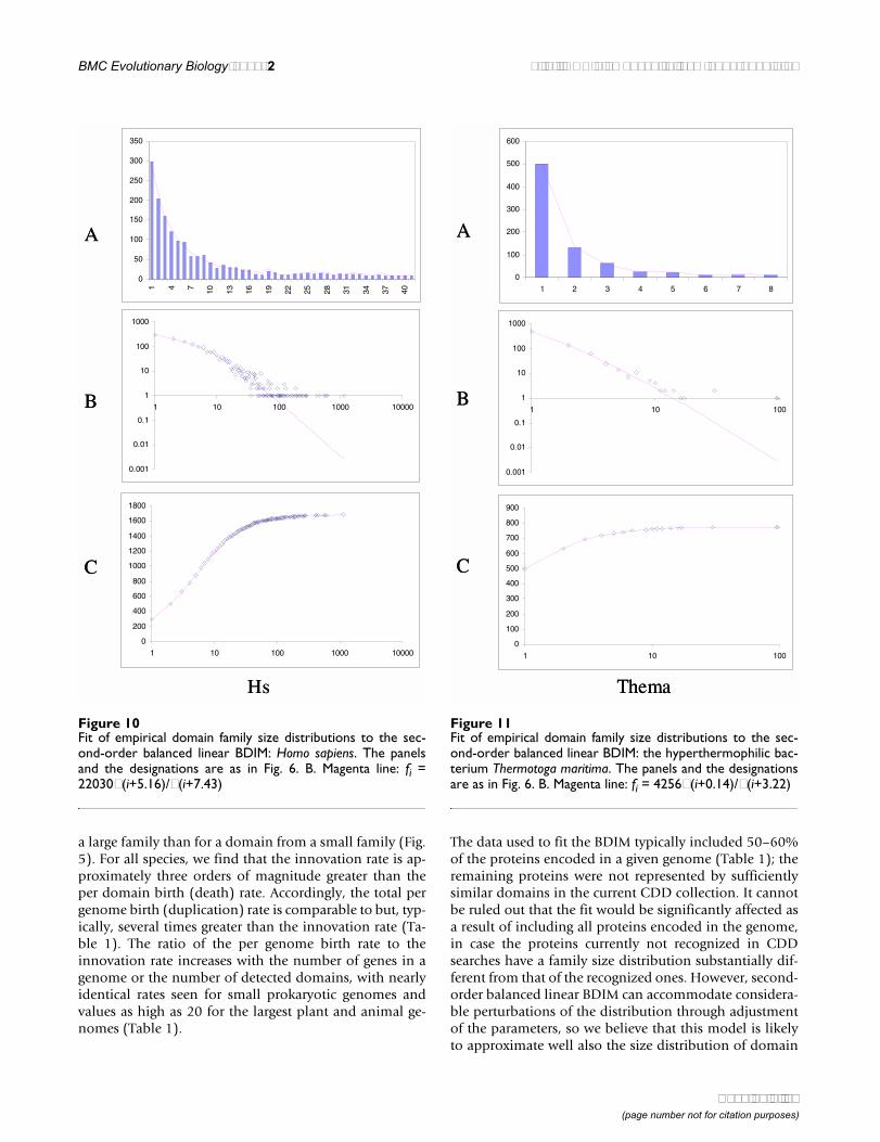
a large family than for a domain from a small family (Fig.5). For all species, we find that the innovation rate is ap-proximately three orders of magnitude greater than theper domain birth (death) rate. Accordingly, the total pergenome birth (duplication) rate is comparable to but, typ-ically, several times greater than the innovation rate (Ta-ble 1). The ratio of the per genome birth rate to theinnovation rate increases with the number of genes in agenome or the number of detected domains, with nearlyidentical rates seen for small prokaryotic genomes andvalues as high as 20 for the largest plant and animal ge-nomes (Table 1).
The data used to fit the BDIM typically included 50–60%of the proteins encoded in a given genome (Table 1); theremaining proteins were not represented by sufficientlysimilar domains in the current CDD collection. It cannotbe ruled out that the fit would be significantly affected asa result of including all proteins encoded in the genome,in case the proteins currently not recognized in CDDsearches have a family size distribution substantially dif-ferent from that of the recognized ones. However, second-order balanced linear BDIM can accommodate considera-ble perturbations of the distribution through adjustmentof the parameters, so we believe that this model is likelyto approximate well also the size distribution of domain
Figure 10Fit of empirical domain family size distributions to the sec-ond-order balanced linear BDIM: Homo sapiens. The panelsand the designations are as in Fig. 6. B. Magenta line: fi =22030Γ(i+5.16)/Γ(i+7.43)
0
50
100
150
200
250
300
3501 4 7 10 13 16 19 22 25 28 31 34 37 40
0.001
0.01
0.1
1
10
100
1000
1 10 100 1000 10000
0
200
400
600
800
1000
1200
1400
1600
1800
1 10 100 1000 10000
A
B
C
Hs
A
B
C
Hs
Figure 11Fit of empirical domain family size distributions to the sec-ond-order balanced linear BDIM: the hyperthermophilic bac-terium Thermotoga maritima. The panels and the designationsare as in Fig. 6. B. Magenta line: fi = 4256Γ(i+0.14)/Γ(i+3.22)
0
100
200
300
400
500
600
1 2 3 4 5 6 7 8
0.001
0.01
0.1
1
10
100
1000
1 10 100
0
100
200
300
400
500
600
700
800
900
1 10 100
A
B
C
Thema
A
B
C
Thema
Page 18 of 26(page number not for citation purposes)
BMC Evolutionary Biology 2002, 2 http://www.biomedcentral.com/1471-2148/2/18
families for complete sets of proteins encoded in a ge-nome. An alternative approach that at least partially cir-cumvents the sampling problem involves analysis of allfamilies of paralogs detectable using clustering by se-quence similarity, with employing a predefined library ofdomains; this analysis is beyond the scope of the presentwork but may be a subject of further investigation.
General discussion and conclusionsHere, we presented a complete mathematical descriptionof the size distribution of protein domain families encod-ed in genomes for simple but not unrealistic models of ev-
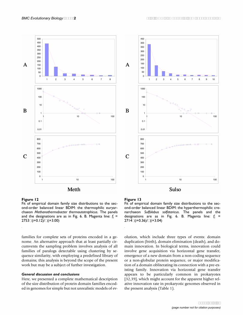
olution, which include three types of events: domainduplication (birth), domain elimination (death), and do-main innovation. In biological terms, innovation couldinvolve gene acquisition via horizontal gene transfer,emergence of a new domain from a non-coding sequenceor a non-globular protein sequence, or major modifica-tion of a domain obliterating its connection with a pre-ex-isting family. Innovation via horizontal gene transferappears to be particularly common in prokaryotes[32,39], which might account for the apparent higher rel-ative innovation rate in prokaryotic genomes observed inthe present analysis (Table 1).
Figure 12Fit of empirical domain family size distributions to the sec-ond-order balanced linear BDIM: the thermophilic euryar-chaeon Methanothermobacter thermautotrophicus. The panelsand the designations are as in Fig. 6. B. Magenta line: fi =2753Γ(i+0.12)/Γ(i+3.00)
0
50
100
150
200
250
300
350
400
450
500
1 2 3 4 5 6 7 8
0.01
0.1
1
10
100
1000
1 10 100
0
100
200
300
400
500
600
700
800
1 10 100
A
B
C
Metth
A
B
C
Metth
Figure 13Fit of empirical domain family size distributions to the sec-ond-order balanced linear BDIM: the hyperthermophilic cre-narchaeon Sulfolobus solfataricus. The panels and thedesignations are as in Fig. 6. B. Magenta line: fi =2714Γ(i+0.36)/Γ(i+3.04)
0
50
100
150
200
250
300
350
400
450
1 2 3 4 5 6 7 8 9 10
0.01
0.1
1
10
100
1000
1 10 100
0
100
200
300
400
500
600
700
800
1 10 100
A
B
C
Sulso
A
B
C
Sulso
Page 19 of 26(page number not for citation purposes)

BMC Evolutionary Biology 2002, 2 http://www.biomedcentral.com/1471-2148/2/18
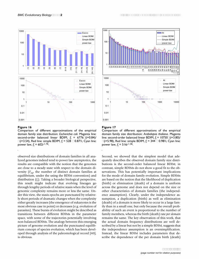
We showed that birth-death-innovation models (BDIMs)with different levels of complexity lead to readily distin-guishable predictions regarding the distribution of do-main family sizes in genomes. In particular, we definedthe exact analytic conditions that lead, exactly or asymp-totically, to power law distributions, which have recentlyreceived ample attention, as they were uncovered in vari-ous biological and social contexts [20,25]. In contrast toprevious analyses [16,17,30] but in agreement with the re-sults of a recent re-examination [31], we showed that thepower law only asymptotically approximates the domainfamily size distributions.
Three groups of observations made in this work seem tohave the greatest potential of enhancing our understand-ing of genome evolution and, perhaps, evolution of othercomplex systems. First, we proved that, within the BDIMframework, there is a unique equilibrium state of the sys-tem, which is approached exponentially, with respect totime, from any initial state. In this equilibrium state, thenumber of domain families in each size class remains con-stant and follows a unique distribution depending on thetype and parameters of the BDIM. In particular, power as-ymptotics emerges when and only when a BDIM is sec-ond-order balanced, i.e. the rates of domain birth anddeath are asymptotically equal. Since we showed that the
Figure 14Fit of empirical domain family size distributions to the sec-ond-order balanced linear BDIM: the bacterium Bacillus subti-lis. The panels and the designations are as in Fig. 6. B.Magenta line: fi = 3489Γ(i+0.48)/Γ(i+3.01)
0
100
200
300
400
500
600
1 2 3 4 5 6 7 8 9 10 11 12 13
0.01
0.1
1
10
100
1000
1 10 100 1000
0
200
400
600
800
1000
1200
1 10 100 1000
A
B
C
Bacsu
A
B
C
Bacsu
Figure 15Fit of empirical domain family size distributions to the sec-ond-order balanced linear BDIM: the bacterium Escherichiacoli. The panels and the designations are as in Fig. 6. B.Magenta line: fi = 6776Γ(i+0.84)/Γ(i+3.54)
0
100
200
300
400
500
600
1 2 3 4 5 6 7 8 9 10 11 12 13
0.01
0.1
1
10
100
1000
1 10 100 1000
0
200
400
600
800
1000
1200
1 10 100 1000
A
B
C
Escco
A
B
C
Escco
Page 20 of 26(page number not for citation purposes)
BMC Evolutionary Biology 2002, 2 http://www.biomedcentral.com/1471-2148/2/18
observed size distributions of domain families in all ana-lyzed genomes indeed tend to power law asymptotics, theresults are compatible with the notion that the genomesare close to a steady state with respect to the domain di-versity (Feq, the number of distinct domain families atequilibrium, under the using the BDIM convention) anddistribution (fi). Taking a broader biological perspective,this result might indicate that evolving lineages gothrough lengthy periods of relative stasis when the level ofgenomic complexity remains more or less the same. Un-der this view, the stasis epochs are punctuated by relative-ly short periods of dramatic changes when the complexityeither greatly increases (the emergence of eukaryotes is themost obvious case in point) or decreases (e.g. evolution ofparasites). These bursts of evolution might be described astransitions between different BDIMs in the parameterspace, with some of the trajectories potentially involvingnon-balanced BDIMs. The analogy between this emergingpicture of genome evolution and the punctuated equilib-rium concept of species evolution, which has been devel-oped through analysis of the paleontological record [40],is obvious.
Second, we showed that the simplest model that ade-quately describes the observed domain family size distri-butions is the second-order balanced linear BDIM; incontrast, simple BDIMs do not show a good fit to the ob-servations. This has potentially important implicationsfor the mode of domain family evolution. Simple BDIMsare based on the notion that the likelihood of duplication(birth) or elimination (death) of a domain is uniformacross the genome and does not depend on the size orother characteristics of domain families (the independ-ence assumption). Clearly, under the independence as-sumption, a duplication (birth) as well as elimination(death) of a domain is more likely to occur in a large fam-ily than in a small one, but only because the overall prob-ability of such an event is proportional to the number offamily members, whereas the birth (death) rate per domainremains the same. The key observation of this work, thatthe actual domain frequency distributions are well de-scribed by a linear but not by a simple BDIM, suggests thatthe independence assumption is an oversimplification.Instead, the linear BDIM includes parameters that de-scribe the dependence of the per domain birth (death)
Figure 16Comparison of different approximations of the empiricaldomain family size distribution: Escherichia coli. Magenta line:second-order balanced linear BDIM, fi = 6776Γ(i+0.84)/Γ(i+3.54), Red line: simple BDIM, fi = 528 × 0.87i/i, Cyan line:power law, fi = 602i-1.76.
1
10
100
1000[1
]
[2]
[3]
[4]
[5]
[6]
[7]
[8..9
]
[10]
[11.
.13]
[14.
.18]
[19.
.23]
[24.
.140
]
Escco
Linear BDIM
Simple BDIM
power-law
0.001
0.01
0.1
1
10
100
1000
1 10 100 1000
Escco
Linear BDIM
Simple BDIM
power-law
Figure 17Comparison of different approximations of the empiricaldomain family size distribution: Arabidopsis thaliana. Magentaline: second-order balanced linear BDIM, fi = 10750Γ(i+3.80)/Γ(i+5.98), Red line: simple BDIM, fi = 344 × 0.98i/i, Cyan line:power law, fi = 516i-1.36.
1
10
100
1000
[1]
[2]
[3]
[4]
[5]
[6]
[7]
[8]
[9]
[10]
[11]
[12]
[13]
[14]
[15]
[16]
[17]
[18.
.19]
[20]
[21]
[22.
.23]
[24.
.25]
[26.
.27]
[28.
.32]
[33.
.35]
[36.
.40]
[41.
.45]
[46.
.50]
[51.
.60]
[61.
.64]
[65.
.75]
[76.
.88]
[89.
.103
][1
04..1
43]
[144
..182
][1
83..1
535]
At
Linear BDIM
Simple BDIM
power-law
0.001
0.01
0.1
1
10
100
1000
1 10 100 1000 10000
At
Linear BDIM
Simple BDIM
power-law
Page 21 of 26(page number not for citation purposes)
BMC Evolutionary Biology 2002, 2 http://www.biomedcentral.com/1471-2148/2/18
rate on the family size. The asymptotics of the theoreticaldistribution that is the best fit for the actual data is a pow-er law, with the power equal to a-b-1, where a and b are theparameters of a linear BDIM. We observed that, for all an-alyzed genomes, a-b-1 < -1 (a <b), which corresponds to"synergy" between domains in a family. Both the domainbirth rate and the death rate drop with the increase of thesize of a domain family, but the death rate decreases faster(Fig. 5). In general terms, this suggests that small familiesare more dynamic during evolution than large families. Inparticular, under the BDIM formalism, innovation con-tributes only to single-member families (class 1), whichhave the greatest evolutionary mobility, and either quick-ly proliferate and are stabilized or perish. An implicationof these observations is that, in general, large families areolder than small ones. Exceptions to this generalization,i.e. the existence of small, ancient families, probably pointto selection for a specific family size; for example, it seemslikely that selection acts against proliferation of certain es-sential proteins, e.g. ribosomal proteins, which typicallyform single-member families [41]. Another pertinent ob-servation is that the linear BDIM seems to adequately ac-commodate even the largest of the identified domainfamilies. Lineage-specific expansion of paralogous fami-lies appears to be one of the principal modes of organis-mic adaptation during evolution [13,14,42]. Thus,quantitatively, adaptive family expansion appears to fitwithin the BDIM framework, although these models donot explicitly incorporate the notion of selection. Ofcourse, for BDIMs, it is irrelevant which families expand,and this choice is determined by selection.
Third, the BDIM equilibrium condition with respect to thetotal number of domain families, ν = δ1f1 (ν is the inno-vation rate, δ1 is the domain death rate for class 1 families,and f1 is the number of domain families in class 1) allowsus to estimate the ratio between domain innovation rateand the domain death and birth rates. Indeed, accordingto the above and the definition of a second-order linearBDIM, which is the best fit for the actual data, λ = δ = ν/f1(1+b). Since the number of domain families in class 1(families with only one member) is in the hundreds foreach genome, this translates into an innovation rate thatis much greater than the duplication or elimination rateper domain (Table 1). Such high innovation rates mightappear counter-intuitive, but let us note that the duplica-tion rate over all domain families is a number that tendsto be nearly identical to ν for small prokaryotic genomesand several-fold greater than ν for large eukaryotic genom-es (Table 1). Thus, under the second-order balanced linearBDIM, the likelihood of appearance of a new domain in agenome is close to or several times less than the likelihoodof a duplication or elimination of an existing domain.Nevertheless, the finding that the innovation rate is com-parable to the overall duplication/elimination rate seems
surprising. If the linear BDIM is indeed a realistic evolu-tionary model, this emphasizes the critical role of innova-tion in maintaining the balance (steady state) in genomeevolution. In prokaryotes, innovation via horizontal genetransfer appears to be particularly extensive [32,39],which might underlie the greater relative innovation ratein these organisms (Table 1).
As already indicated, BDIMs do not explicitly incorporateselection. However, the present analysis shows that onlymodels with precisely balanced domain birth, death andinnovation rates can account for the observed distributionof domain family size in each of the analyzed genomes. Itseems likely that the balance between these rates is itself aproduct of selection. There is little doubt that BDIMs willbe eventually replaced by more sophisticated formalismsthat will more realistically capture the mechanisms of ge-nome evolution. Nevertheless, even the crude modelingdescribed here seems to reveal several potentially interest-ing and non-trivial aspects of the evolutionary process.
Mathematical Appendix. Proofs of some statementsProof of Proposition 1When system (3.1) is solved consecutively from the lastequation to the second one, it becomes obvious that thesolution is unique up to a constant multiplier.
Next, if fi = fi-1λi-1/δi, fi+1 = fi-1λi-1λi/(δiδi+1), then the sub-stitution shows that (fi-1,fi,fi+1) satisfy the i-th equation ofsystem (3.2). Substituting f2 = f1λ1/δ2 in the first equation,
we get f1 = ν/δ1 and, consequently,
for all i = 2,...N. By definition, Feq = fi, so we have
(3.3).
Since system (2.2) is linear, the equilibrium state (f1,...fN)is asymptotically stable if the real parts of all characteristicvalues of the matrix
are negative.
The following theorem (see [43]) gives the desired criteri-on: the real part of all the characteristic values of a real ma-
f vi kk
i
kk
i=
=
−
=∏ ∏λ δ
1
1
1
/
i
N
=∑
1
AN =
− +( )− +( )
λ δ δλ λ δ δ1 1 2
1 2 2 3
0 0
0 0
... ... ... ... ...
... ... ... ...
.... ... ... ... ... ... ... ... ...
... ...
... ...
0 0 0 01 1λ λ δ δi i i i− +− +( ).... ... ... ... ... ... ...
... ... ... ...
...
0 0
02 1 1λ λ δ δN N N N− − −− +( )
.... ... ... ... 0 1λ δN N− −
Page 22 of 26(page number not for citation purposes)
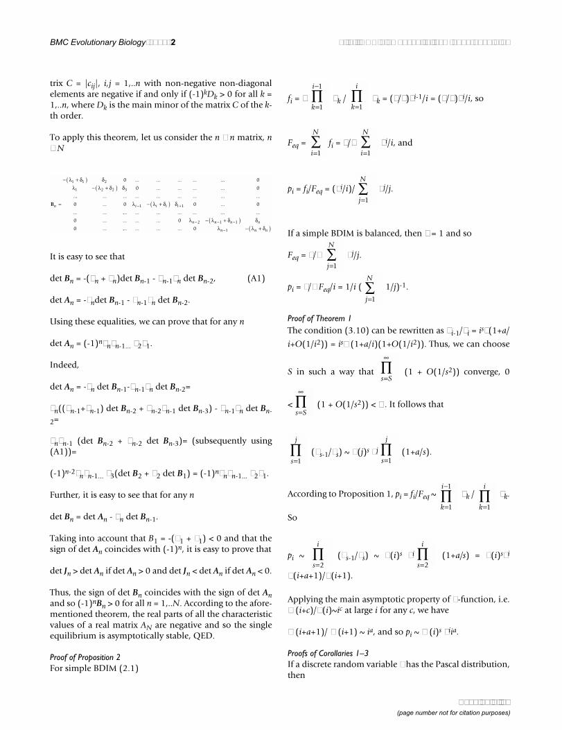
BMC Evolutionary Biology 2002, 2 http://www.biomedcentral.com/1471-2148/2/18
trix C = |cij|, i,j = 1,..n with non-negative non-diagonalelements are negative if and only if (-1)kDk > 0 for all k =1,..n, where Dk is the main minor of the matrix C of the k-th order.
To apply this theorem, let us consider the n × n matrix, n≤ N
It is easy to see that
det Bn = -(λn + δn)det Bn-1 - λn-1δn det Bn-2, (A1)
det An = -δndet Bn-1 - λn-1δn det Bn-2.
Using these equalities, we can prove that for any n
det An = (-1)nδnδn-1... δ2δ1.
Indeed,
det An = -δn det Bn-1-λn-1δn det Bn-2=
δn((λn-1+δn-1) det Bn-2 + λn-2δn-1 det Bn-3) - λn-1δn det Bn-
2=
δnδn-1 (det Bn-2 + λn-2 det Bn-3)= (subsequently using(A1))=
(-1)n-2δnδn-1... δ3(det B2 + λ2 det B1) = (-1)nδnδn-1... δ2δ1.
Further, it is easy to see that for any n
det Bn = det An - λn det Bn-1.
Taking into account that B1 = -(λ1 + δ1) < 0 and that thesign of det An coincides with (-1)n, it is easy to prove that
det Jn > det An if det An > 0 and det Jn < det An if det An < 0.
Thus, the sign of det Bn coincides with the sign of det Anand so (-1)nBn > 0 for all n = 1,..N. According to the afore-mentioned theorem, the real parts of all the characteristicvalues of a real matrix AN are negative and so the singleequilibrium is asymptotically stable, QED.
Proof of Proposition 2For simple BDIM (2.1)
fi = ν λk / δk = (ν/δ)θi-1/i = (ν/λ)θi/i, so
Feq = fi = ν/λ θi/i, and
pi = fi/Feq = (θi/i)/ θj/j.
If a simple BDIM is balanced, then θ = 1 and so
Feq = ν/λ θj/j.
pi = ν/λ Feq/i = 1/i ( 1/j)-1.
Proof of Theorem 1The condition (3.10) can be rewritten as λi-1/δi = isθ(1+a/
i+O(1/i2)) = isθ (1+a/i)(1+O(1/i2)). Thus, we can choose
S in such a way that (1 + O(1/s2)) converge, 0
< (1 + O(1/s2)) < ∞. It follows that
(λs-1/δs) ~ Γ(j)s θj (1+a/s).
According to Proposition 1, pi = fi/Feq ~ λk / δk.
So
pi ~ (λs-1/δs) ~ Γ(i)s θi (1+a/s) = Γ(i)sθi
Γ(i+a+1)/Γ(i+1).
Applying the main asymptotic property of Γ-function, i.e.Γ (i+c)/Γ(i)~ic at large i for any c, we have
Γ (i+a+1)/ Γ (i+1) ~ ia, and so pi ~ Γ (i)s θiia.
Proofs of Corollaries 1–3If a discrete random variable ξ has the Pascal distribution,then
Bn =
− +( )− +( )
λ δ δλ λ δ δ1 1 2
1 2 2 3
0 0
0 0
... ... ... ... ...
... ... ... ...
.... ... ... ... ... ... ... ... ...
... ...
... ...
0 0 0 01 1λ λ δ δi i i i− +− +( ).... ... ... ... ... ... ...
... ... ... ...
...
0 0
02 1 1λ λ δ δn n n n− − −− +( )
.... ... ... ... 0 1λ λ δn n n− − +( )
k
i
=
−
∏1
1
k
i
=∏
1
i
N
=∑
1 i
N
=∑
1
j
N
=∑
1
j
N
=∑
1
j
N
=∑
1
s S=
∞
∏
s S=
∞
∏
s
j
=∏
1 s
j
=∏
1
k
i
=
−
∏1
1
k
i
=∏
1
s
i
=∏
2 s
i
=∏
2
Page 23 of 26(page number not for citation purposes)

BMC Evolutionary Biology 2002, 2 http://www.biomedcentral.com/1471-2148/2/18
P(ξ = i) 1 / Γ (r) (1-q)rir-1qi ~ qiir-1 for large i,
and it becomes evident that, for a > -1, equilibrium fre-quencies pj of the first-order balanced BDIM follow thePascal distribution with parameters (a+1,θ).
If a = -1, then pi ~ θi/i and so pi follows the truncated log-arithmic distribution with parameter θ. If a = 0, then pj ~θi and pi follows the geometric distribution.
Further, pi ~ ia, that is the sequence pi follows the powerdistribution with the power a, if and only if θ = 1, that is,if the BDIM is second-order balanced.
Finally, if λi-1/δi = 1 + O(1/i2), that is, if θ = 1 and a = 0,then pi ~ const; in particular, if λi-1 = δi for all i, then, ac-cording to Proposition 1, fi = ν for all i and pi = 1/N.
Proof of Theorem 2According to Proposition 1, system (3.1) has the uniquesolution:
f1 = νδ1, fi = ν λs / δs for all i = 2,...N. So
fi = ν/λθi P(s) / Q(s), i > 1.
Applying the Lemma (see below), we get
fi Cν/λ θi Γ (i)ηiρ-β, as i→∞,
where the constant C = [(Γ(1+bk))^βk] /
[Γ(1+ak)^αk].
Lemma. Let P(j) = (j+ak)^αk, Q(j) = (j+bk)^βk,
where ak, bk are positive. Let us denote
η = αk - βk, ρ = ak αk - bkβk, β =
βk,.
Then with fixed j
N(j) = P(s) / Q(s) C Γ(j)ηj^(ρ-β)
as j→∞, where
C = [(Γ(1+bk))^βk] / [Γ(1+ak)^αk].
Proof.
(s+ak)^αk = [Γ(j+ak) / Γ(1+ak)]^αk,
(s+bk)^βk = [Γ(j+1+bk) / Γ(1+bk)]^βk, so
N(j) = { [Γ(j+ak) / Γ(1+ak)]^αk}/{ [Γ(j+1+bk)/
Γ(1+bk)]^βk}=
C [(Γ(j+ak))^αk]/ [(Γ(j+1+bk))^βk]
where
C = [(Γ(1+bk))^βk]/ [Γ(1+ak)^αk].
Let us use the known asymptotic relation
Γ (t+a)/Γ (t) ta with t→∞.
Thus we have
[(Γ(j+ak))^αk]/ [(Γ(j+1+bk))^βk]
(Γ(j))η [(Γ(j+ak) / Γ(j))^αk] / [(Γ(j+1+bk) /
Γ(j))^βk]
(Γ(j))ηj^[ ak αk] / j^[ (bk+1)βk]=
(Γ(j))ηj^(ρ-β),
≅
s
i
=
−
∏1
1
s
i
=∏
1
s
i
=
−
∏1
1
s
i
=∏
1
≅
k
m
=∏
1 k
n
=∏
1
k
n
=∏
1 k
m
=∏
1
k
n
=∑
1 k
m
=∑
1 k
n
=∑
1 k
m
=∑
1
k
m
=∑
1
s
j
=
−
∏1
1
s
j
=∏
1≅
k
m
=∏
1 k
n
=∏
1
s
j
=
−
∏1
1
s
j
=∏
1
k
n
=∏
1 k
m
=∏
1
k
n
=∏
1 k
m
=∏
1
k
m
=∏
1 k
n
=∏
1
≅
k
n
=∏
1 k
m
=∏
1
k
n
=∏
1 k
m
=∏
1
≅
k
n
=∏
1 k
m
=∏
1
Page 24 of 26(page number not for citation purposes)
BMC Evolutionary Biology 2002, 2 http://www.biomedcentral.com/1471-2148/2/18
and Lemma is proved.
Proof of Proposition 3It follows from the proof of the Lemma that
fi = Cν/λ θi [(Γ(j+ak))^αk] / [(Γ(j+1+bk))^βk]
for i > 1,
where C = [(Γ(1+bk))^βk] / [(Γ(1+ak))^αk].
Let us show that f1 can be expressed by the same formulaif i = 1. Indeed,
Cν/δ [(Γ(1+ak))^αk] / [(Γ(1+1+bk))^βk=
ν/δ ( (Γ(1+bk))^βk / (Γ(1+ak))^αk)) (
(Γ(1+ak))^αk / (Γ(2+bk))^βk=
ν/δ ( (Γ(1+bk))^βk / (Γ(2+bk))^βk = ν/δ (
(1+bk))^βk = f1
Thus,
Feq = Cν/δ ( θj-1 (Γ(j+ak))^αk/
(Γ(j+1+bk))^βk).
QED.
Contributions of individual authorsGPK developed most of the mathematical formalism andwrote the draft of the mathematical part of the manu-script; YIW performed the identification of domain in se-quenced genomes and the statistical analysis of theresulting distributions and wrote the draft of the corre-sponding part of the manuscript; FSB proved some of thetheorems; AYR largely incepted the work and contributedto the formulation of the models; EVK contributed to theinception of the work and the formulation of the models,gave the biological interpretation of the results, wrote the
background and discussion sections and extensively edit-ed the entire manuscript.
AcknowledgementsWe thank Alexei Kondrashov, Alexei Ogurtzov, and Vladimir Ponomarev for critical reading of the manuscript and the Koonin group members for helpful discussions.
References1. Koonin EV, Aravind L, Kondrashov AS: The impact of compara-
tive genomics on our understanding of evolution. Cell 2000,101:573-576
2. Lander ES, Linton LM, Birren B, Nusbaum C, Zody MC, Baldwin J,Devon K, Dewar K, Doyle M, FitzHugh W, Funke R, Gage D, HarrisK, Heaford A, Howland J, Kann L, Lehoczky J, LeVine R, McEwan P,McKernan K, Meldrim J, Mesirov JP, Miranda C, Morris W, Naylor J,Raymond C, Rosetti M, Santos R, Sheridan A, Sougnez C, Stange-Thomann N, Stojanovic N, Subramanian A, Wyman D, Rogers J, Sul-ston J, Ainscough R, Beck S, Bentley D, Burton J, Clee C, Carter N,Coulson A, Deadman R, Deloukas P, Dunham A, Dunham I, DurbinR, French L, Grafham D, Gregory S, Hubbard T, Humphray S, HuntA, Jones M, Lloyd C, McMurray A, Matthews L, Mercer S, Milne S,Mullikin JC, Mungall A, Plumb R, Ross M, Shownkeen R, Sims S, Wa-terston RH, Wilson RK, Hillier LW, McPherson JD, Marra MA, MardisER, Fulton LA, Chinwalla AT, Pepin KH, Gish WR, Chissoe SL, WendlMC, Delehaunty KD, Miner TL, Delehaunty A, Kramer JB, Cook LL,Fulton RS, Johnson DL, Minx PJ, Clifton SW, Hawkins T, BranscombE, Predki P, Richardson P, Wenning S, Slezak T, Doggett N, Cheng JF,Olsen A, Lucas S, Elkin C, Uberbacher E, Frazier M, et al: Initial se-quencing and analysis of the human genome. Nature 2001,409:860-921
3. Dacks JB, Doolittle WF: Reconstructing/deconstructing theearliest eukaryotes: how comparative genomics can help. Cell2001, 107:419-425
4. Chervitz SA, Aravind L, Sherlock G, Ball CA, Koonin EV, Dwight SS,Harris MA, Dolinski K, Mohr S, Smith T, Weng S, Cherry JM, BotsteinD: Comparison of the complete protein sets of worm andyeast: orthology and divergence. Science 1998, 282:2022-2028
5. Rubin GM, Yandell MD, Wortman JR, Gabor Miklos GL, Nelson CR,Hariharan IK, Fortini ME, Li PW, Apweiler R, Fleischmann W, CherryJM, Henikoff S, Skupski MP, Misra S, Ashburner M, Birney E, BoguskiMS, Brody T, Brokstein P, Celniker SE, Chervitz SA, Coates D,Cravchik A, Gabrielian A, Galle RF, Gelbart WM, George RA, Gold-stein LS, Gong F, Guan P, Harris NL, Hay BA, Hoskins RA, Li J, Li Z,Hynes RO, Jones SJ, Kuehl PM, Lemaitre B, Littleton JT, Morrison DK,Mungall C, O'Farrell PH, Pickeral OK, Shue C, Vosshall LB, Zhang J,Zhao Q, Zheng XH, Zhong F, Zhong W, Gibbs R, Venter JC, AdamsMD, Lewis S: Comparative genomics of the eukaryotes. Science2000, 287:2204-2215
6. Koonin EV, Tatusov RL, Rudd KE: Sequence similarity analysis ofEscherichia coli proteins: functional and evolutionary implica-tions. Proc Natl Acad Sci U S A 1995, 92:11921-11925
7. Brenner SE, Hubbard T, Murzin A, Chothia C: Gene duplicationsin H. influenzae. Nature 1995, 378:140
8. Labedan B, Riley M: Widespread protein sequence similarities:origins of Escherichia coli genes. J Bacteriol 1995, 177:1585-1588
9. Tatusov RL, Mushegian AR, Bork P, Brown NP, Hayes WS, Boro-dovsky M, Rudd KE, Koonin EV: Metabolism and evolution ofHaemophilus influenzae deduced from a whole-genomecomparison with Escherichia coli. Curr Biol 1996, 6:279-291
10. Ponting CP, Schultz J, Milpetz F, Bork P: SMART: identificationand annotation of domains from signalling and extracellularprotein sequences. Nucleic Acids Res 1999, 27:229-232
11. Bateman A, Birney E, Cerruti L, Durbin R, Etwiller L, Eddy SR, Grif-fiths-Jones S, Howe KL, Marshall M, Sonnhammer EL: The Pfamprotein families database. Nucleic Acids Res 2002, 30:276-280
12. Marchler-Bauer A, Panchenko AR, Shoemaker BA, Thiessen PA, GeerLY, Bryant SH: CDD: a database of conserved domain align-ments with links to domain three-dimensional structure. Nu-cleic Acids Res 2002, 30:281-283
13. Jordan IK, Makarova KS, Spouge JL, Wolf YI, Koonin EV: Lineage-specific gene expansions in bacterial and archaeal genomes.Genome Res 2001, 11:555-565
k
n
=∏
1 k
m
=∏
1
k
m
=∏
1 k
n
=∏
1
k
n
=∏
1 k
m
=∏
1
k
m
=∏
1 k
n
=∏
1 k
n
=∏
1
k
m
=∏
1
k
m
=∏
1 k
m
=∏
1 k
m
=∏
1
j
N
=∑
1 k
n
=∏
1 k
m
=∏
1
Page 25 of 26(page number not for citation purposes)
BMC Evolutionary Biology 2002, 2 http://www.biomedcentral.com/1471-2148/2/18
14. Lespinet O, Wolf YI, Koonin EV, Aravind L: The role of lineage-specific gene family expansion in the evolution of eukaryo-tes. Genome Res 2002, 12:1048-1059
15. Aravind L, Watanabe H, Lipman DJ, Koonin EV: Lineage-specificloss and divergence of functionally linked genes in eukaryo-tes. Proc Natl Acad Sci U S A 2000, 97:11319-11324
16. Huynen MA, van Nimwegen E: The frequency distribution ofgene family sizes in complete genomes. Mol Biol Evol 1998,15:583-589
17. Qian J, Luscombe NM, Gerstein M: Protein family and fold occur-rence in genomes: power-law behaviour and evolutionarymodel. J Mol Biol 2001, 313:673-681
18. Rzhetsky A, Gomez SM: Birth of scale-free molecular networksand the number of distinct DNA and protein domains pergenome. Bioinformatics 2001, 17:988-996
19. Wuchty S: Scale-free behavior in protein domain networks.Mol Biol Evol 2001, 18:1694-1702
20. Barabasi AL: Linked: The New Science of Networks. New York: PerseusPr 2002
21. Barabasi AL, Albert R: Emergence of scaling in random net-works. Science 1999, 286:509-512
22. Albert R, Barabasi AL: Statistical mechanics of complex net-works. Reviews of Modern Physics 2002, 74:47-97
23. Albert R, Jeong H, Barabasi AL: Error and attack tolerance ofcomplex networks. Nature 2000, 406:378-382
24. Amaral LA, Scala A, Barthelemy M, Stanley HE: Classes of small-world networks. Proc Natl Acad Sci U S A 2000, 97:11149-11152
25. Gisiger T: Scale invariance in biology: coincidence or footprintof a universal mechanism? Biol Rev Camb Philos Soc 2001, 76:161-209
26. Jeong H, Mason SP, Barabasi AL, Oltvai ZN: Lethality and central-ity in protein networks. Nature 2001, 411:41-42
27. Jeong H, Tombor B, Albert R, Oltvai ZN, Barabasi AL: The large-scale organization of metabolic networks. Nature 2000,407:651-654
28. Dorogovtsev SN, Mendes JF: Scaling properties of scale-freeevolving networks: Continuous approach. Phys Rev E Stat PhysPlasmas Fluids Relat Interdiscip Topics 2001, 63:056125
29. Krapivsky PL, Redner S: Organization of growing random net-works. Phys Rev E Stat Phys Plasmas Fluids Relat Interdiscip Topics 2001,63:066123
30. Luscombe N, Qian J, Zhang Z, Johnson T, Gerstein M: The domi-nance of the population by a selected few: power-law behav-iour applies to a wide variety of genomic properties. GenomeBiol. 2002, 3:research0040.0041-0040.0047
31. Kuznetsov VA: Statistics of the numbers of transcripts andprotein sequences encoded in the genome. In: 'Computationaland Statistical Approaches to Genomics (Edited by: Zhang W, ShmulevichI) Boston: Kluwer 2002, 125-171
32. Koonin EV, Makarova KS, Aravind L: Horizontal gene transfer inprokaryotes: quantification and classification. Annu Rev Micro-biol 2001, 55:709-742
33. Feller W: An introduction to probability theory and its application. NewYork: Wiley 1967–1968
34. Ijuri Y, Simon HA: Skew distributions and the sizes of business firms. Am-sterdam, New York, Oxford: North-Holland Publishing Company 1977
35. Gihman II, Skorohod AV: The theory of stochastic processes. New-York,Heidelberg, Berlin: Springer-Verlag 1975
36. Johnson NL, Kotz S, Kemp AW: Univariate discrete distributions. NewYork: Wiley 1992
37. Henrici P: Applied and computational complex analysis. New York: Wiley1986
38. Wolf YI, Grishin NV, Koonin EV: Estimating the number of pro-tein folds and families from complete genome data. J Mol Biol2000, 299:897-905
39. Lawrence JG, Ochman H: Amelioration of bacterial genomes:rates of change and exchange. J Mol Evol 1997, 44:383-397
40. Gould SJ: The Structure of Evolutionary Theory. Cambridge, MA: HarvardUniv. Press 2002
41. Tatusov RL, Galperin MY, Natale DA, Koonin EV: The COG data-base: a tool for genome-scale analysis of protein functionsand evolution. Nucleic Acids Res 2000, 28:33-36
42. Remm M, Storm CE, Sonnhammer EL: Automatic clustering oforthologs and in-paralogs from pairwise species compari-sons. J Mol Biol 2001, 314:1041-1052
43. Gantmacher FR: The theory of matrices. New York: Chelsea PublishingCompany 1989
Publish with BioMed Central and every scientist can read your work free of charge
"BioMedcentral will be the most significant development for disseminating the results of biomedical research in our lifetime."
Paul Nurse, Director-General, Imperial Cancer Research Fund
Publish with BMC and your research papers will be:
available free of charge to the entire biomedical community
peer reviewed and published immediately upon acceptance
cited in PubMed and archived on PubMed Central
yours - you keep the copyright
[email protected] your manuscript here:http://www.biomedcentral.com/manuscript/
BioMedcentral.com
Page 26 of 26(page number not for citation purposes)
Copyright © 2022 FDOKUMEN