REVIEWS OF GEOPHYSICS AND SPACE PHYSICS, VOL. 21, NO. 1, PAGES 41-50, FEBRUARY 1983

Applications of Deformation Analysis in Geodesy and Geodynamics ATHANA$IOS DERMANI$ AND EVANGELOS LIVIERATO$

Higher Geodesy and Cartography, Faculty of Engineering, University of Thessaloniki Thessaloniki, Greece

The role of deformation analysis is discussed with respect to its existing or possible future applications in geodesy and geodynamics. Expressions for strain tensors are given in the more general case of Riemannian spaces and specialized for Euclidean spaces and the case of infinitesimal deformation. Among the various applications, special emphasis is given to the study of crustal deformations of the earth, deformations of the gravity field, and gravity field related deformations. Other applications are also considered.

INTRODUCTION

Deformation, loosely speaking, is the alteration of form and shape. Deformation is historically linked to the study of de- formable material bodies, originally within the theory of elas- ticity and later on within continuum mechanics [Love, 1927; Malvern, 1969; Truesdell, 1977; Erin•len, 1980]. The abstrac- tion of relevant concepts and mathematical tools developed in mechanics leads to their broader use in a variety of problems which are not related to material bodies.

Since form and shape are connected to the metric character- istics of bodies, deformation, in a broad sense, is also concerned with the alteration of such characteristics of general physical or even abstract entities. It is only necessary that the elements of such entities can be brought into a one-to-one correspondence, in the same way that through the identification of material points a correspondence is established between two different states of a deformable body.

Applying deformation analysis in the geosciences, for exam- ple, in geodesy, the previous discussion meets a clear example: From its definition, geodesy studies among other topics the material shape and the gravity field of the earth as well as their alteration in space and time. The earth body deformation cor- responds to the classical treatment in mechanics of deformable bodies, while the deformation of the gravity field of the earth calls for an abstract application of the same tools. Another, even more obvious, example of abstract deformation is illus- trated by mapping the geographic grid of parallels and meri- dians from the globe onto a plane grid, a standard technique in cartography; the spherical and plane grids under comparison are obviously abstract entities of a nonmaterial nature.

In mechanics, deformation (strain) is not studied by itself but mainly in connection with the underlying forces (stress-strain relation). Although the forces acting to cause earth deformation are of interest in both geodesy and geophysics, geodesists are primarily concerned with the development of methods and techniques for the determination of such deformation.

The object of geodesy is the study of the size, shape, and gravity field of the earth, position determination, time variation of all the above, and their representation. Consequently, defor- mation methods find manifold applications in geodetic work.

Copyright 1983 by the American Geophysical Union.

Paper number 2R1568. 0034-6853/83/002R- 1568515.00

41

MATHEMATICAL TOOLS

Since form and shape are described mathematically by the concept of metric, deformation can be represented by math- ematical objects which depend on metric alterations.

Usually, in classical mechanics the relevant metric spaces are Euclidean. This is due to the model accepted for the description of the physical three-dimensional space in the neighborhood of the earth. The most convenient way of describing Euclidean space is by means of Cartesian orthogonal coordinate systems. However, curvilinear coordinates within Euclidean spaces are also useful in some applications.

In order to apply the above mathematical techniques outside the realm of mechanics, a generalization to Riemmanian metric spaces is sometimes necessary, for example, in cartographic applications.

Therefore the development of our formulation will start from curvilinear Riemmanian spaces. Euclidean descriptions with curvilinear or Cartesian coordinate systems will then be derived as special cases.

The Riemmanian Case

Let there be two Riemmanian spaces with corresponding metrics dS 2 and ds 2 which describe their metrical properties in the infinitesimal neighborhood of points of the two spaces. Curvilinear coordinate systems (U x U 2 U 3) and (u x u 2 u 3) are assigned to the two spaces. The metrics with respect to the chosen coordinate system are given by

dS2 -- Z GiJ dUi dUJ = dUTG dU (1) ij

ds2 = Y'• •lij du i duJ= durg du (2)

where Gij, gid are the corresponding metric tensors and G, g their matrix representations.

It is furthermore assumed that a one-to-one correspondence exists between the two spaces described by

u = u(U) (3)

This mapping function must also be continuous and have a continuous inverse, that is, a homeomorphism in mathematical terms. In classical mechanics the sets U and u(U) correspond to the same point in two different states of a material body.

For the description of deformations we look at the differ- ences (ds 2- dS 2) between corresponding elements of the two spaces under comparison. These differences can be expressed either in terms of the first coordinate system U (Lagrangian approach) or in terms of the second coordinate system u (Eu- lerian approach).

42 DERMANIS AND LIVIERATOS' DEFORMATION IN GEODESY/GEODYNAMICS

When the Lagrangian approach is followed, the Lagrangian strain tensor (strain matrix) E is introduced by means of

ds: - dS: ae=f 2dUr E dU (4)

It follows that

E = «[(•u/•U)•g(•u/•U) - a] (5)

When the Eulerian approach is followed, the Eulerian strain tensor (strain matrix) E* is introduced by means of

ds 2 _ dS • ae__f 2durE, du (6)

so that

E* = «[g - (•U/•u)rG(•U/•u)] (7)

We have called E and E* in (5) and (7) tensors. However, some clarifications are needed. Tensors obey well-known trans- formation rules under changes of coordinate systems. These rules apply to E and E* when the first coordinate system U undergoes a transformation, while the second coordinate system u undergoes the corresponding transformation induced by (3). On the one hand, function (3) depends on an underlying correspondence between the elements of the two compared Riemmanian spaces; on the other hand, its specific mathemat- ical representation is a consequence of the more or less arbi- trary selection of the coordinate systems U and u. A general discussion of this aspect is given by Boucher [1980]. The point will be clarified later when specific applications are analyzed.

Note that all components of the strain tensor must have the same physical dimensions. The reason for this restriction is that scalar invariants of the strain tensor are sometimes used as

deformation parameters. Since these invariants (i.e., the trace and determinant) are combinations of the tensor components, they are physically meaningful when the particular components have the same physical dimensions. Recalling (4), the above restriction necessitates the use of curvilinear coordinates of the

same physical units in contrast to some usual choices (e.g., spherical coordinates with both angular and linear units). In order to avoid this inconvenience, all coordinates may be trans- formed to coordinates of the same units through multiplication with suitable scalar factors. For example, when angular coordi- nates are used in the same set with linear coordinates, they can be transformed to linear ones through multiplication with the radii of curvature of the corresponding coordinate lines.

Equation (4) can be written as

ds2/dS 2 a½=f 1 + 2(dUT/dS)E(dU/dS) (8)

or

rnL2 a•f 1 + 2LrEL (9)

where mL is the linear modulus of deformation along the direc- tion of the unit vector L - dU/dS. Replacing LrL = 1 in (9), we obtain

mL 2 = LT(I + 2E)L (10)

which represents a quadratic form. The associated quadric surface, being the geometric locus of all points with m• • = 1, is the well-known Cauchy strain ellipsoid in three dimensions or the Tissot strain ellipse in two dimensions used in cartography.

In the usual description of this quadratic form, the restriction that all curvilinear coordinates in U be of the same physical dimension is relaxed, and (9) is now written as

mr, 2 = 1 + 2LrKEKL (11)

where K is the diagonal matrix with elements the correspond- ing curvatures of the coordinate lines. Similarly, (10) becomes

rnL: = Lr(K: + 2KEK)L (12)

The Euclidean Case

In the special but common case where the spaces under comparison are Euclidean, it is always possible to assign global orthogonal Cartesian coordinate systems, e.g., (X • X: X 3) and (x • x 2 x3). Then the corresponding metrics become

dS2 = dX r dX (13)

ds 2 = dx T dx (14)

that is, the metric tensors become identity (G = g = I). For a given one-to-one correspondence

x = x(X)

the Langrangian and Eulerian strain tensors become

E = «[-(c3x/c3X)r(c3x/c3X)- I] (16)

E* = «El -(•X/•x)r(&X/&x)J (17)

It is also possible to describe Euclidean spaces by curvilinear orthogonal coordinate systems, e.g., (Q• Q: Qa) and (q• q: qa). In this case the metrics are written as

dS • = dQrC dQ (18)

ds • = dqre dq (19)

Comparison with (13) and (14) gives

C = (c3X/c3Q)r(c3X/c3Q) (20)

e = (c3x/c3q)r(c3x/c3q) (21)

Similar expressions in tensor notation are given by Hotine [1969].

For a given one-to-one correspondence

q = q(Q) (22)

the Lagrangian and Eulerian strain tensors are

E = «[C - (c3q/c3Q)rc(c3q/c3Q)] (23)

E* = «[(c9Q/c9q)rc(c9Q/c9q) - e] (24)

All the above derivations hold equally well for any dimen- sions, but our applications are limited to two and three dimen- sions.

Strain tensors are powerful tools in studying deformations, for they allow a pointwise illustration of alteration of the metric properties. In particular, the tensor field E(U) describes defor- mation in the infinitesimal vicinity of each element of the first space with coordinates (U • U: U3). E*(u) does the same for elements of the second space.

Infinitesimal Deformation

When deformations are small, the transformation u = u(U) is a transformation close to the identity. In this case the displace- ments (• •2 •3)

DERMANIS AND LIVIERATOS: DEFORMATION IN GEODESY/GEODYNAMICS 43

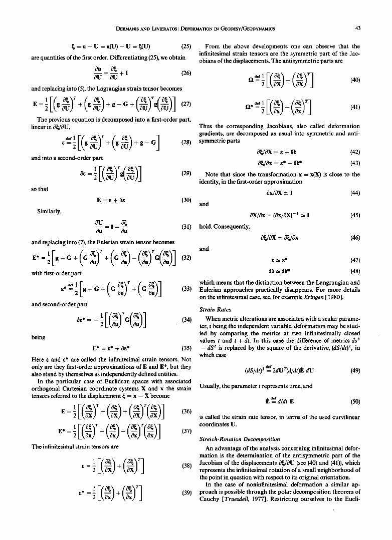
g = u - u = u(U)- u = g(u)

are quantities of the first order. Differentiating (25), we obtain

0u - + I (26)

8U 8U

and replacing into (5), the Lagrangian strain tensor becomes

The previous equation is decomposed into a first-order part, linear in a•/aU,

e=• g0uJ + g• +g-G (28) and into a second-order part

so that

Similarly,

E = e + & (30)

ou o• -I (31)

Ou Ou

and replacing into (7), the Eulerian strain tensor becomes

E'= -1 [g-G+ (G 2•U•)T + (G 2•u)--(a•U•)TG(2"•I (32, 2 kau/]

with first-order part

•,=• g-g+ • + • (33) and second-order part

being

(34)

E* = •* + &* (35)

Here • and •* are called the infinitesimal strain tensors. Not

only are they first-order approximations of E and E*, but they also stand by themselves as independently defined entities.

In the particular case of Euclidean spaces with associated orthogonal Cartesian coordinate systems X and x the strain tensors referred to the displacement • = x - X become

The infinitesimal strain tensors are

(38) •=• • +k•x/_l

1 •*=• • (39)

From the above developments one can observe that the infinitesimal strain tensors are the symmetric part of the Jac- obians of the displacements. The antisymmetric parts are

(40)

n,=• • kax/1 (41)

Thus the corresponding Jacobians, also called deformation gradients, are decomposed as usual into symmetric and anti- symmetric parts

8•/0X = •; + f• (42)

0•,/0x = e* + f•* (43)

Note that since the transformation x = x(X) is close to the identity, in the first-order approximation

and

hold. Consequently,

0x/SX -• I (44)

and

0X/0x = (0x/0X)- • •_ • (45)

O•/OX -• •,/•x (46)

• -• •* (47)

fI •' fI* (48)

which means that the distinction between the Langrangian and Eulerian approaches practically disappears. For more details on the infinitesimal case, see, for'example Eringen [ 1980].

Strain Rates

When metric alterations are associated with a scalar parame- ter, t being the independent variable, deformation may be stud- ied by comparing the metrics at two infinitesimally closed values t and t + dt. In this case the difference of metrics ds 2 -dS 2 is replaced by the square of the derivative, (dS/dr) 2, in

which case

(dS/dt)2 ae__r 2dUr(d/dt) œ dU (49)

Usually, the parameter t represents time, and

a/at E (50)

is called the strain rate tensor, in terms of the used curvilinear coordinates U.

Stretch-Rotation Decomposition

An advantage of the analysis concerning infinitesimal defor- mation is the determination of the antisymmetric part of the Jacobian of the displacements 8g/0U (see (40) and (41)), which represents the infinitesimal rotation of a small neighborhood of the point in question with respect to its original orientation.

In the case of noninfinitesimal deformation a similar ap- proach is possible through the polar decomposition theorem of Cauchy [Truesdell, 1977]. Restricting ourselves to the Eucli-

44 DERMANIS AND LIVIERATOS'. DEFORMATION IN GEODESY/GEODYNAMICS

dean case, the Jacobian of the displacements can be uniquely decomposed in two ways,

c•g/c•X = RVs = Vt.R (51)

where R is an orthogonal matrix called the rotation matrix and VR, VL are positive symmetric matrices called the right and the left stretch matrices, respectively. The rotation matrix repre- sents the change of orientation of a small neighborhood of the point in question.

The independent elements of R can be computed from the displacement Jacobian matrix by solving one of the following rather complicated matrix equations:

= \ox/j ox

DEFORMATION OF THE EARTH

General Discussion

As is well known, geodetic observations are of a geometric and physical nature. They are also limited to points on and/or outside the surface of the earth. It is beyond the scope of this paper to discuss deformation problems related to the interior of the earth [Bullen, 1975], since such deformations do not signifi- cantly affect geodetic observations. On the contrary, defor- mations of the crust are directly connected with geodetic ob- servables. Geometric observations are related to the alteration

of the two-dimensional surface of the crust as embedded into

three dimensions.

Deformations of the crust, beyond the surface, cause changes in the gravity field of the earth and can be sensed through gravity-dependent geodetic observations.

It must be noted that changes in the gravity vector and gravity potential at discrete points of the surface can be ascribed either to the surface motion or to changes in the gravity field per se. These two effects can be separated when the whole surface is covered by observations, in which case geo- dynamic boundary value problems are formulated for the de- termination of variation in the geometry of the boundary sur- face and variations of the gravity field outside the surface [see Dermanis and Sans& 1982' Heck, 1981].

The study of global deformations of the crust surface can be primarily done by space geodetic techniques (laser ranging, very long baseline interferometry, etc.), while traditional geod- etic techniques (triangulation, trilateration) are valuable for the study of deformations on a local scale. Global crust defor- mation and plate tectonic motion determination are the subject of extensive research both theoretical and applied, but there are still problems to be solved (for a discussion see, for example, Baarda [1975] and Livieratos [ 1979]).

Local crustal deformation studies are referred to two dimen-

sions, following the classical separation of geodetic practice, that is, the duality planimetry-elevation. In this case, leveling is tied through gravity with internal changes. Since height is anholonomic, that is, path-dependent, geopotential numbers must rather be used through the combination of leveling with

(e.g., crust embedded in a Euclidean space) it is necessary to know the continuous field of displacements at every point of the medium or, at least, in the neighborhood of specific points where strain is to be calculated (see (36) and (37)).

Geodetic observations are usually discrete and limited to points on the two-dimensional surface. Even if the three com- ponents of the displacement vectors in a network of surface points could be evaluated by analyzing geodetic observations, strains could not be directly computed. In order to evaluate the space derivatives of displacements appearing in (36) and (37) a continuous field of displacements is needed. When only discrete values of displacements are available, a continuous field •(X) can be obtained by interpolation. The interpolation concerns the determination of displacements not only on the surface but also within and outside the crust. For points within the crust the strains are computed by analytically differentiating the interpolated function •,(X), and consequently, the strains depend not only on the discrete geodetic observations but also on the chosen interpolation technique. The more the interpola- tion technique reflects physical reality, the closer the computed strains are to the real ones.

The same holds for strain computation at points on the crust surface, but an additional problem exists: In physical reality, displacements outside the medium are not defined, and stress- strain relation problems can be faced, introducing boundary conditions on the surface. •

Mathematically speaking, interpolation techniques predict displacements even outside the medium, and computed surface strains depend on such predictions and consequently do not reflect physical reality. They have only a descriptive value and should not be used, for example, for conclusions on stress-strain relations.

In practice, the problems connected with deformations in three dimensions are bypassed by computing separately two- dimensional plane strains and vertical motions. Since it is natu- ral to be interested in three-dimensional deformations, one may think of combining two-dimensional plane displacements with vertical motions in order to derive displacements in three di- mensions and the relevant strains. However, as already men- tioned, vertical motions are severely dependent on changes of the gravity field even when these changes are not accompanied by motion of the terrestrial surface.

As is well known to geodesists, the really estimable quantities are differences of the geopotential, which can be transformed into orthometric height differences and into their time vari- ations only when the gravity field and its time variation are independently known.

On the other hand, the effect of the gravity field variations on the plane horizontal coordinates of triangulation points is neg- ligible. When analyzing a local triangulation network, a common horizontal plane of reference is assumed for the per- pendicular projection of network points. In this case, though observations (angular horizontal measurements) at each point depend on the local direction of the plumb line, they are not sensitive to the expected small changes in this direction. This allows the determination of horizontal displacements which

gravity. Geopotential differences may be caused by changes of essentially reflect actual horizontal motions with negligible ef- the gravity field due to density redistributions within the crust without any actual change of the geometric shape of the sur- face. A discussion of the discrepancies between actual and apparent height differences as related to crustal movement is given by Bird[1975].

In order to compute strains in a three-dimensional medium

fects from gravity field variations. Works and discussions related to the above can be found in

several collective volumes [e.g., Pavoni and Green, 1975; Riki- take, 1976, 1981; Mueller, 1978; Hieber and Guyenne, 1978; Vogel, 1979; NASA, 1979, 1980, 1981; lsikara and Vogel, 1981; U.S. National Research Council, 1981].

DERMANIS AND LIVIERATOS' DEFORMATION IN GEODESY/GEODYNAMICS 45

For vertical movements and associated gravity variations see, for example, Faytel'son and Yurkina [1974], Yurkina [1977], Hein [1978], Drewes [1980], and Vanicek et al. [1980].

Further elaborations with emphasis on analysis are given by Brunner [1979], Kumar [1979], Wassef [1979], Brunner et al. [1981], Dermanis [1981], Hein and Kistemann [1981], Kelm [1981], Koch and Fritsch [1981], Livieratos and Vlachos [1981], and Niemeier [1981].

Two-Dimensional Plane Strain

For the study of crustal deformations in two dimensions, usually followed in practice, intrinsic two-dimensional strains are defined for the description of the geometric alterations in the positions of the projections of the surface points onto the local reference plane.

Again, as in the three-dimensional case, strains, being local differential quantities, require continuous displacement infor- mation. Geodetic techniques provide only discrete displace- ments, and strains can be computed only after an explicit or implicit interpolation of displacements.

The definitions of the Lagrangian strain tensor E, the infini- tesimal strain tensor a, the infinitestimal rotation matrix 11, and their Eulerian counterparts apply equally well in the two- dimensional case. Since the analysis is carried out on the plane (Euclidean space), the equations (36)-(41) are appropriate.

The numerical values of strain tensor elements depend on the reference frame used. Thus one should look for scalar functions

of the strain tensor elements which are invariant with respect to the chosen reference frame and moreover have an evident

physical interpretation. It is well known that there exists a particular reference frame with respect to which the strain tensor, being symmetric, takes a diagonal form:

Ae = [E; ax E0minl (53) The quantities Emax, Emi n are called the (Lagrangian) prin-

cipal strains. In order to compute the principal strains from the components of the strain tensor

Exy E = [•• Ey•l (54) in any two-dimensional Cartesian coordinate system, well- known spectral techniques must be applied. Indeed, the prin- cipal strains Emin, Ema x are the eigenvalues of E and can be computed as the roots of the characteristic equation

det (E - XI) = X 2 - tr (E)X + det (E) = 0 (55)

which are

,•1: Emax -- «{tr (E) + [tr (E) 2 - 4 det (E)] •/2 }

,•2 = Emin = «{tr (E) - [tr (E) 2 - 4 det (E)] •/2 } (56)

The scalar quantities

A = Ema x + Emi n

y = Ema x -- Emi n (57)

are called the dilatation and the maximum shear strain, respec- tively. A represents the isotropic part and 7 the anisotropic part of deformation in the infinitesimal vicinity of the point of interest. They are both point functions with the following physical interpretation: A is the areal change per unit area

(positive for an increase in area), and 7 is the shear across the direction of its maximum value (always positive).

The scalar invariants A and 7 can be expressed, according to Truesdell and Noll [1965], in terms of the so-called principal invariants Ix(E ) and I2(E), which in the two-dimensional case are

I•(E) = tr (E) I2(E) = det(E) (58)

Combination of (56) with (57) gives

A = I•(E)= tr (E)= E•o, + Eyy

72 = I•2(E) - 412(E) = [tr (E)] 2 - 4 det (E) (59)

= (gxx -- gyy) 2 q- (2E,,,) 2

Introducing the shear components

7 • = E,,x- Eyy (60)

72 = 2E•,y (61)

the maximum shear strain becomes

2 2)•/2 (62) 7=(7• + 72

The above shear components have the following interpretation [Prescott et al., 1979]'7 • is the shear across any line parallel to the y direction (north), and 72 is the shear across any line parallel to the x direction (east).

The azimuth of the maximum extension Ema x is computed from the eigenvector problem

where

En = •n (63)

n = [sin Lcos •] (64) Eliminating 3. from (63), it follows that

arctan (-72/7•) (65)

When the infinitesimal strain a only is considered, corre- sponding infinitesimal quantities A, 7, etc. are defined.

From the Jacobian of the displacements (46), the infinitesi- mal antisymmetric rotation matrix

is also defined, where ro is the angle (in radians) of infinitesimal rotation. Similar quantities are analogously defined for the Eulerian mode of description.

There is an extensive literature concerning applications of the above two-dimensional plane strain analysis from geodetic results. Two approaches are basically followed. In the first approach, angular or distance observations at two different epochs are used (observation methods). In the second ap- proach, the coordinates from independently adjusted triangu- lations at two epochs are used (coordinate method). This is essentially a finite element method where strains are considered constant within the triangular elements.

Concerning horizontal deformations see, for example, Frank [1966], Sato [1973], Bibby [1975, 1981], Savage [1976], Pre- scott [1976], Harada [1977], Gerasimenko et al. [1977], Liv- ieratos [1978, 1980], Baldi et al. [1979], Cohen and Cook [1979], Harada and Shimura [1979], Nyland et al. [1979], Prescott et al. [1979], Reilly [1979], Savage et al. [1979], Snay

46 DERMANIS AND LIVIERATOS' DEFORMATION IN GEODESY/GEODYNAMICS

and Cline [1980], Vlachos [1980], Baldi and Marson [1981], Cacon [1981], Dermanis et al. [1981], Lisowski and Thatcher [1981], and Bencini et ai. [1982].

DEFORMATION OF THE GRAVITY FIELD OF THE EARTH

AND GRAVITY FIELD RELATED DEFORMATIONS

As already discussed in the introduction, while the analysis in the previous chapter concerned the classical treatment of ma- terial deformation, the same tools can be abstracted for the study of deformations related to the gravity field of the earth.

In this context, three alternative cases are studied: 1. The most straightforward way of defining deformation of

the gravity field is to compare two different gravity vector fields in the vicinity of a fixed point in geometry space.

2. Since traditionally in geodesy we deal with positioning by means of observations related to the gravity field, an alter- native approach can be formulated by studying the change of geometric positions identified by the same value of the gravity vector, or any three other appropriate gravity field related parameters, with respect to two different gravity fields under comparison.

3. The third alternative is to study the alterations of the geometric and gravity characteristics, as well as their inter- relation, in the vicinity of material points of the earth's surface.

For the study of these cases the following Jacobians are used:

•F/•X = B •F/•x = • (67)

O¾/OX = b O¾/Ox = [I

where x and X are the 'old' and 'new' position vectors, respec- tively, and ¾ and F the corresponding gravity vectors.

Gravity Deformation at Fixed Space Position

Let us consider a point X fixed in geometry space and two different potential fields W and w assigning corresponding gravity vectors F = grad W(X) and ¾ = grad w(X). Since F and ¾ are Cartesian coordinates in gravity space, they can be used for the definition of gravity strain in the same way that the space Cartesian coordinates are used in (16) and (17) for the definition of geometry strains. The Lagrangian gravity strain is

E(F) = «[(c•¾/•F)r(•¾/•F) - I] (68)

and the Eulerian gravity strain is

W*(•): «r• - (or/o•)qor/o•)] (69)

In the more general case when curvilinear coordinates •(F) and 9(¾) are used for the description of gravity space, the above relations are written as in (5) and (7),

w

X-=x--z ,F

w

X--x

E(•) = «[(c•q•/&•)rm(c•q•/&•)- M] (70)

E(q•) = «[m - (c•/&q•)rM(&•/&q•)] (71)

m, M being the metric tensors associated with the curvilinear frames used. Since gravity space is Euclidean,

m = drd M = DrD (72)

where

d = c•¾/c•9 D = c•F/c•b (73)

Introducing the matrices of second-order space derivatives of the potential (gravity gradients),

1• (•W• T cqF &f cqF &f c•Xk,•XJ -c•X - B- c•x - • (74)

exkx/ -ex- b-ox- II the gravity strain tensors referred to Cartesian coordinates become

E(F) = «(B-'b2B -' - I) (76)

E*(y) = «(I - b- 'B2b - ') (77)

and the gravity strain tensors referred to curvilinear coordi- nates are

E(•) = «[DrB - •b(d- ')rind- •bB- •D - M]

and

= «[DrB - •bZB - •D - DrD] (78)

E*(9) = «[drd - drb - •Bab - •d] (79)

Comparing with (76) and (77),

E(•) = DrE(F)D (80)

E*(q•) = dVE(y)d (81)

in agreement with the well-known tensor transformation rules. The two potential fields under comparison could be either

the actual instantaneous fields of the earth at two distinct

epochs or the actual field and a model field (normal potential).

Deformation of Geometry Space at Fixed Gravity

This case is dual to the previous one, since it follows by simply interchanging geometry with gravity space'

w

X ,F--¾

w

x ,F---¾

The situation now is as follows: Consider a position X and a potential field W assigning a gravity vector F = grad W(X). For a second potential field w there exists a position x such that the same gravity vector F = grad w(x) is assigned. In this abstract way, positions X and x are brought to one-to-one correspondence, in the same way that in continuum mechanics, positions are paired as positions of the same material point at different epochs.

The strain tensors are thus defined as in (16) and (17):

E(X) = «[(E•x/•X)T(•x/•X)- I]

E*(x) = «[I - (•X/•x)T(•X/•x)]

(82)

(83)

Introducing the matrices of second-order derivatives of the potential,

Txxkax / Txx = I=Txx (84)

DERMANIS AND LIVIERATOS' DEFORMATION IN GEODESY/GEODYNAMICS 47

the strain tensors become

E(x) = «(Bp-•B - I) (85)

E*(x) = «(I - liB-:P) (86)

Generalizations can be easily derived for the case when curvilinear coordinates are used in geometry space.

An application of the above treatment is found in the case where W is the actual potential of the earth and w the normal potential. In this case, x is the image of X under the telluroid mapping X •-• x defined by

grad w(x)= grad W(X) (87)

The relevant strain tensors (85) and (86) describe deformation induced by, for example, mapping the surface of the earth into the telluroid [Bocchio, 1976, 1979a, b; Osada, 1978, 1980; Marussi, 1973, 1974; Grafarend, 1978a, 1978b; Teisseyre, 1969].

A similar analysis can be carried out by identifying positions through their natural coordinates ß = ((I) A W/wo) T or normal coordinates q• = (•p 2 W/Wo) T instead of the gravity vectors F or •/, respectively, where Wo is a reference constant with potential dimension, that is, a reference normal potential value. The choice of pure numbers W/w o and w/w o instead of the corre- sponding potentials W and w is suggested in order to obtain strain tensor components of the same units.

w

X ,•-=q•

w

x ,•--q•

The strain tensors are defined exactly as in (16) and (17) or (82) and (83). Introducing the matrices

F = O•/0X f = 0•/Ox (88)

the strain tensors become

E(X) = «[Fr(ffr) - •F -- I] (89)

E*(x) = «[I - fT(FFT)-'f] (90)

This case finds application in studying deformations induced by the telluroid mapping X •-• x defined by

v(x) = w(x) (91)

grad w(x) grad W(X)

I grad w(x)l I grad W(X)[

The Apparent Gravity Deformations

The case most closely connected to observational reality concerns the change of the gravity field at material points which is due to both change of the gravity field itself and change of position due to motion of the surface of the earth. The situation can be shown as

w

P-•X

w

P-•x '7

where X and x are two different positions of the same material point P and F and ? the corresponding apparent (observable) gravity vectors induced by two different potential fields W and W.

The geometry strain tensors E(X) and E(x) are defined as in

(16) and (17) or (82) and (83). Introducing the matrix of second- order derivatives of the potential

B = •?r/•?X (92)

and recalling definition (75), we obtain

c•X - •? OF gX - p • B (93) Thus the strain tensors become

E(X)=•L k•] •B-I (94)

E,(x) = 5 - Similar expressions can be derived for the case where instead

of F and • the natural coordinates ß and •, respectively, are available.

Earth Tidal Deformation

A particular case of the previous formulation concerns the deformation of the earth's crust associated with the lunisolar

tides. A material point in a relaxed state has a position X, and the potential W is due only to earth attraction and rotation. An additional potential reflecting lunisolar attraction leads to a new disturbed state where the material point moves to a new position x and the final potential w depends on the original potential, the potential of the lunisolar attractions, and the variations caused by mass redistribution after elastic yielding. The final position x of any material point is a function of its original position X, the original and final potential W and w, and a set of parameters (Love and Shida numbers). In conse- quence, strains depend on the above function. For derivations of tidal strains, see Melchior [1978]. For an interesting appli- cation see Marussi [ 1979].

OTHER APPLICATIONS

A case completely analogous to the temporal variation of network coordinates caused by crustal deformation is the one where two coordinate sets of the same time-invariant network

are available from different sources. Typical examples are the inconsistencies in coordinates as derived from classical adjust- ment and space techniques (see, for example, Mueller [1974]), differences in coordinates as adjusted on a reference ellipsoid and on a projective plane, coordinate differences between the results of compatible adjustments based on data from different observational campaigns, coordinate differences in common parts of networks, alterations in the form of a lower-order network when superfluous, fixed, higher-order control points are used, etc. The physical meaning of deformation in such cases varies with each particular application.

When three-dimensional coordinates from space techniques are compared with classical ellipsoidal geodetic coordinates, deformation parameters may be related to systematic errors caused, for example, when normal parameters of the gravity field are used instead of their actual values in the classical

procedures of reduction of the actual observations to the refer- ence surface [Meissl, 1973; Thomson et al., 1974].

Another example is the comparison of two forms of a net- work (or parts of a network) resulting from the utilization of different subsets of the total originally available observations, in which case, deformation parameters may be used for the

48 DERMANIS AND LIVIERATOS: DEFORMATION IN GEODESY/GEODYNAMICS

detection of gross observation inconsistencies (blunders) [Thapa, 1980; Vanicek et al., 1981].

A very interesting aspect of the study of deformation appears in engineering surveying [Pelzer, 1971, 1974; Platek, 1974; Van Mierlo, 1977; Hailerman, 1981], which concerns the temporal alterations in the shape of man-made structures. Beyond the need for generalization to three dimensions we notice the possi- bility of relating observed strains with stresses, since the elastic behavior of such structures are more or less known.

A simple two-dimensional Euclidean case is the study of film deformation in photogrammetric applications.

A well-known two-dimensional case is the deformation in-

volved in cartographic projections, when original figures on a Riemmanian space (sphere or ellipsoid) are deformed into cor- responding figures on a Euclidean space (plane map) (see, for example, Marussi [1951a, b, 1959], Bernasconi [1953, 1956], Caputo [1956], Bocchio [1969], Chovitz [1979], Hojovec and Jokl [1981], and Dermanis and Livieratos [ 1982]).

Other geodetic applications involving comparison of figures in two-dimensional Riemmanian spaces are the study of defor- mations occurring in mapping the geoid onto the reference ellipsoid and similar comparisons between alternative choices of reference ellipsoids (see, for example, Marussi [1951a, b, 1957], O'Keefe [1953], Caputo [1959], and Zadro and Carmin- elli [ 1966]).

Since deformation parameters are connected to comparison of metrics, one can study deformation between different metri- zations of one and the same physical space, without the need of establishing point-to-point correspondences. An example can be found in the study of atmospheric refraction, where the three-dimensional Euclidean earth space is compared with itself when endowed with a metric related to the index of refraction

(see, for example, Marussi [1953] and Grafarend [1975]). A related approach is based on the exploitation of certain

analogies between stress-strain relations of elasticity theory and error propagation in geodetic networks [Borre and Krarup, 1974; Grafarend, 1977; Borre, 1979].

REFERENCES

Baarda, W., Difficulties in establishing a model for testing crustal movements, in Progress in Geodynamics, pp. 45-51, North-Holland, Amsterdam, 1975.

Baldi, P., and I. Marson, Gravity and geodetic networks for the study of crustal deformations in seismic area (Ancona), Boll. Geod. Sci. Affini, 40(3), 189-196, 1981.

Baldi, P., D. Postpischl, M. Unguendoli, and E. Boschi, Strain measurements in the Ancona area, in Optimization of Design and Computation of Control Networks, edited by F. Halmos and J. So- mogyi, pp. 17-22, Akademiai Kiado, Budapest, 1979.

Bencini, P., A. Dermanis, E. Livieratos, and D. Rossikopoulos, Crustal deformation at the Friuli area from discrete and continuous geodetic prediction techniques, Boll. Geod. Sci. Affini, 41(2), 137-148, 1982.

Bernasconi, C., Carte geografiche secondo il modello della membrana elastica, Geofis. Pura Appl., 26, 16-19, 1953.

Bernasconi, C., Rappresentazioni parziali e totali dell' ellissoide di rotazione sulla sfera, Geofis. Pura Appl., 33, 1-8, 1956.

Bibby, H. M., Crustal strain from triangulation in Marlborough, New Zealand, Tectonophysics, 29, 529-540, 1975.

Bibby, H. M., Geodetically determined strain across the southern end of the Tonga-Kermadec-Hikurangi subduction zone, Geophys. J. R. Astron. Soc., 66, 513-533, 1981.

Bir6, P., Vertical crustal movements and time changes of the gravity field, paper presented at Symposium on Recent Crustal Movement, XVIth General Assembly, Int. Union of Geod. and Geophys., Gre- noble, France, 1975.

Bocchio, F., Sui campi di curve superficiali a transformata geodetica nelle rappresentazioni cartografiche di tipo generale, Rend. Accad. Naz. Lincei, Set. VIII, 46(2), 92-96, 1969.

Bocchio, F., Linear and angular deformations in three-dimensional

potential invariant representations of the actual gravity field of the earth and applications, Geophys. J. R. Astron. Soc., 46, 155-164, 1976.

Bocchio, F., Three-dimensional representations of the geopotential field and related topics, Boll. Geod. Sci. Affini, 38(1), 25-43, 1979a.

Bocchio, F., Isoparametric and isozenithal type representations of the actual gravity field of the earth, Geophys. J. R. Astron. Soc., 57, 343-351, 1979b.

Borre, K., Elasticity and stress-strain relations in geodetic networks, Boll. Geod. Sci. Affini, 38(3), 417-456, 1979.

Borre, K., and T. Krarup, Foundation of a theory of elasticity for geodetic networks, paper presented at 7th Nordiske Geodaetm4de, Copenhagen, May 6-10, 1974.

Boucher, C., The general theory of deformation and its applications in geodesy, Boll. Geod. Sci. Affini, 39(1), 13-35, 1980.

Brunner, F. K., On the analysis of geodetic networks for the determi- nation of the incremental strain tensor, Surv. Rev., 25, 192, 1979.

Brunner, F. K., R. Coleman, and B. Hirsch, A comparison of compu- tation methods for crustal strains from geodetic measurements, Tec- tonophysics, 71,281-298, 1981.

Bullen, K. E., The Earth's Density, Chapman and Hall, London, 1975. Cacon, S., Local spatial network as a fragment of the system of geod-

etic networks for complex observation of crustal movement, Sci. Bull. Stanislaw Staszic Univ. Min. Metall., no. 842,67, 65-80, 1981.

Caputo, M., Su alcuni problemi al contorno della teoria delle ra- presentazioni conformi, Atti Ist. Veneto Sci. Lett. Arti, 115, 9-21, 1956.

Caputo, M., Conformal projection of an ellipsoid of revolution when the scal• factor and its normal derivative are assigned on a geodesic line of the ellipsoid, J. Geophys. Res., 64(11), 1867-1873, 1959.

Chovitz, B. H., A general theory of map projections, Boll. Geod. Sci. Affini, 38(3), 457-479, 1979.

Cohen, S.C., and G. R. Cook, Determining crustal strain rates with spaceborne geodynamics ranging system data, Manuscr. Geod., 4, 245-260, 1979.

Dermanis, A., Geodetic estimability of crustal deformation parameters, Quat. Geod.,2(2), 159-169, 1981.

Dermanis, A., and E. Livieratos, Dilatation, shear, rotation and energy analysis of map projections, Boll. Geod. Sci. Affini, in press, 1982.

Dermanis, A., and F. Sans6, The geodynamic boundary value problem, Boll. Geod. Sci. Affini, 41(1), 65-87, 1982.

Dermanis, A. E., Livieratos, D. Rossikopoulos, and E. Vlachos, Geod- etic prediction of crustal deformations at the seismic area of Volvi, in Proceedings of the International Symposium on Geodetic Networks and Computations, Munich, 31 Aug.-5 Sept. 1981, vol. 5, pp. 234-248, Deutsche Geodaetische Kommission, Munich, 1981.

Drewes, H., Problems related to earthquake premonitory gravity ob- servations, Boll. Geofis. Teor. Appl., 22(88), 261-268, 1980.

Eringen, A. C., Mechanics of Continua, R. E. Krieger, New York, 1980. Faytel'son, A. Sh., and M. I. Yurkina, On secular variation of gravity

and recent vertical crustal movements, Geod. Mapp. Photogramm, Engl. Transl., •6(3), 168-171, 1974.

Frank, F. C., Deduction of earth strains from survey data, Bull. Seismo- I. Soc. Am.,56(1), 35-42, 1966.

Gerasimenko, M. G., V. V. Zlotin, and Ya. V. Naumov, A study of recent movements of the earth's crust by geodetic methods (from conference materials), Geod. Mapp. Photogramm., Engl. Transl., 19(3),152-155,1977.

Grafarend, E., Three-dimensional geodesy, III, Refraction, Proc. Hot- line Syrup. Math. Geod.,6th, 105-112, 1975.

Grafarend, E., Stress-strain relations in geodetic networks, Commun. Geod. Inst. Uppsala Univ., no. 16, 1977.

Grafarend, E., Dreidimensionale geod•itische Abbildungsgleichungen und die N•iherungsfigur der Erde, Z. Vermess., 103, 132-140, 1978a.

Grafarend, E., The definition of the telluroid, Bull. Geod., 52, 25--37, 1978b.

Hailermann, L. (Ed.), Proceedings of the II. International Symposium of Deformation Measurements by Geodetic Methods, Bonn, Sept. 25-28, 1978, K. Wittwer, Stuttgart, 1981.

Harada, T., Quiet and violence in horizontal movement of the crust, J. Phys. Earth, 25, suppl., S79-S83, 1977.

Harada, T., and M. Shimura, Horizontal deformation of the crust in western Japan revealed from first-order triangulation carried out three times, Tectonophysics, 52, 469-478, 1979.

Heck, B., Combination of leveling and gravity data •or detecting real crustal movements, in Proceedings of the International Symposium on Geodetic Networks and Computations, Munich, 31 Aug.-5 Sept., 1981,

DERMANIS AND LIVIERATOS: DEFORMATION IN GEODESY/GEODYNAMICS 49

vol. 7, pp. 20-30, Deutsche Geodaetische Kommission, Munich, 1981.

Hein, G., Requirements and statistics of modern levelling networks with respect to vertical crustal movements, in Proceedings of the 2nd International Symposium on Problems Related to the Redefinition of North American Geodetic Networks, pp. 629-636, U.S. Department of Commerce, Washington, D.C., 1978.

Hein, G., and R. Kistemann, Mathematical foundation of non-tectonic effects in geodetic recent crustal movement models, Tectonophysics, 71, 315-334, 1981.

Hieber, S., and T. D. Guyenne (Eds.), Space Oceanography, Navigation and Geodynamics: Proceedings of ESA European Workshop, Elmau, European Space Agency, Paris, 1978.

Hojovec, ¾., and L. Jokl, Relation between the extreme angular and areal distortion in cartographic representation, Stud. Geophys. Geod., 25, 132-151, 1981.

Hotine, M., Mathematical Geodesy, ESSA Monogr., U.S. Department of Commerce, Washington, D.C., 1969.

Isikara, A.M., and A. Vogel (Eds.), Multidisciplinary Approach to Earthquake Prediction, Vieweg, Wiesbaden, Federal Republic of Germany, 1981.

Kelm, R., A geometric-gravimetric estimation procedure for most accu- rate determination of relative point displacements in local areas-- Proposal and first study of sensitivity, in Multidisciplinary Approach to Earthquake Prediction, edited by A.M. Isikara and A. Vogel, ¾ieweg, Wiesbaden, Federal Republic of Germany, 1981.

Koch, K.-R., and D. Fritsch, Multivariate hypothesis tests for detecting recent crustal movements, Tectonophysics, 71, 301-313, 1981.

Kumar, M., Significance of/• error in the assessment of crustal move- ments, Surv. Mapp., 39(2), 133-136, 1979.

Lisowski, M., and W. Thatcher, Geodetic determination of horizontal deformation associated with the Guatemala earthquake of 4th Feb- ruary 1976, Bull. Seismol. Soc. Am., 71(3), 845-856, 198!.

Livieratos, E., Techniques and problems in geodetic monitoring of crustal movements at tectonically unstable regions, paper presented at International Workshop on Monitoring Crustal Dynamics in Earthquake Zones, Eur. Seismol. Comm. and Eur. Geophys. Soc., Strasbourg, Aug. 29 to Sept. 5, 1978. (Published in Terrestrial and Space Techniques in Earthquake Prediction Research, edited by A. Vogel, pp. 515-530, ¾ieweg, Wiesbaden, Federal Republic of Ger- many, 1979.)

Livieratos, E., On the error analysis of geodetically derived strains in seismic zones, Eur. Space Agency Spec. Publ., ESA SP 149, 27-32, 1978.

Livieratos, E., Crustal deformation from geodetic measurements, Boll. Geofis. Teor. Appl., 22(88), 255-260, 1980.

Livieratos, E., and D. ¾1achos, The influence of correlations in com- puting crustal strains from trigonometric network results, Tec- tonophysics, 77, 323-332, 1981.

Love, A. E. H., The Mathematical Theory of Elasticity, Cambridge University Press, New York, 1927.

Malvern, L. E., Introduction to the Mechanics of a Continuum Medium, Prentice-Hall, Englewood Cliffs, N.J., 1969.

Marussi, A., Sulla rappresentazione del geoide sull' ellisoide, Boll. Geod. Soc. Affini, 10(3), 1-7, 195 la.

Marussi, A., Determinazione a priori del modulo di deformazione lineare nella rappresentazione conforme di Gauss, Rend. Accad. Naz. Lincei, Ser. VIII, 11, 3-4, 195 lb.

Marussi, A., Un' analogia fra le leggi della propagazione della luce in mezzi rifrangenti continui isotropi, e le rappresentazioni conformi, Atti Fond. Giorgio Ronchi Contrib. 1st. Naz. Ottica, 8(1), 1953.

Marussi, A., Sulle rappresentazioni fra superfici definite mediante la forma quadratica che ne determina il modulo di deformazione, in Festschrift C.F. Baeschlin, pp. 201-210, Zt/tich, 1957. (Also available as Publ. 33, Ist. di Topogr. e Geod., Univ. di Trieste, Trieste, Italy.)

Marussi, A., Une nouvelle position dans la theorie des cartes geogra- phiques, Commun. Observ. R. Belg., no. 152, Ser. Geophys., no 49, 1959.

Marussi, A., On the three-dimensional computation of geodetic net- works and anomalies, Rend. Accad. Naz. Lincei, Ser. VIII, 55, 5, 1973.

Marussi, A., On the representation of the actual gravity field of the earth on the normal ellipsoidal field, Geophys. J. R. Astron. Soc., 37, 347-352, 1974.

Marussi, A., The tidal field of a planet and the related intrinsic refer- ence systems, Geophys. J. R. Astron. Soc., 56, 409-417, 1979.

Meissl, P., Distortion of terrestrial networks caused by geoid errors,

Proc. Symp. Math. Geod. 5th, 41-52, 1973. Melchior, P., The Tides of the Planet Earth, Pergamon, New York,

1978.

Mueller, I. I., Review of problems associated with conventional geod- etic datums, Can. Surv., 28(5), 514-523, 1974.

Mueller, I. I., (Ed.), Applications of Geodesy to Geodynamics, Pro- ceedings of the 9th GEOP Conference, Rep. 280, Dep. of Geod. Sci., Ohio State Univ., Columbus, 1978.

NASA, Application of space technology to crustal dynamics and earth- quake research, NASA Tech. Pap., 1464, 1979.

NASA, NASA geodynamics program: Annual report for 1979, NASA Tech. Memo., 81978, 1980.

NASA, NASA geodynamics program: Annual report for 1980, NASA Tech. Memo., 84010, 1981.

Niemeier, W., Statistical tests for detecting movements in repeatedly measured geodetic networks, Tectonophysics, 71, 335-351, 1981.

Nyland, E., et al., Measurement and analysis of ground movement using microgeodetic networks on active faults, Geofis. lnt., 18(1), 53-71, 1979.

O'Keefe, J. A., The isoparametric method of mapping one ellipsoid on another, Eos Trans. AGU, 34(6), 869-875, 1953.

Osada, E., Non-conformal transformations of three-dimensional geod- etic networks, Boll. Geod. Sci. Affini, 37(4), 635-649, 1978.

Osada, E., Deformation of geodetic networks in gravity invariant and potential invariant representations, Bull. Geod., 54, 510-520, 1980.

Pavoni, N., and R. Green, Recent Crustal Movements, Elsevier, New York, 1975.

Pelzer, H., Zur Analyse geodaetisher Deformationsmessungen, Rep. C164, Dtsch. Geod. Komm., Munich, 1971.

Pelzer, H., Neuere Ergebnisse bei der statistischen Analyse von Defor- mationsmessungen, in Proceedings of the 14th International Congress of Surveyors, pap. 608.3, Washington, D.C., 1974.

Platek, A., On the application of geodetic methods in the measure- ments of spatial deformations of structures, in Proceedings of the 14th International Congress of Surveyors, pap. 604.1, Washington, D. C., 1974.

Prescott, W. H., An extension of Frank's method for obtaining crustal shear strains from survey data, Bull. Seismol. Soc. Am., 66(6), 1847- 1853, 1976.

Prescott, W. H., J. C. Savage, and T. Kinoshita, Strain accumulation rates in the western United States between 1970 and 1978, J. Geo- phys. Res., 84(B10), 5423-5435, 1979.

Reilly, W. I., Determination of geometric and gravimetric earth defor- mation parameters from geodetic observations, Rep. 140, Geophys. Div., Dep. of Sci. and Ind. Res., Wellington, New Zealand, 1979.

Rikitake, T., Earthquake Prediction, Elsevier, New York, 1976. Rikitake, T. (Ed.), Current Research in Earthquake Prediction, vol. I, D.

Reidel, Hingham, Mass., 1981. Sato, H., A study of horizontal movement of the earth crust associated

with destructive earthquakes in Japan, Bull. Geogr. Surv. Inst., 19(1), 89-130, 1973.

Savage, J. C., Geodetic measurements of crustal motions, The Changing World of Geodetic Science, Rep. 250, pp. 99-118, Dep. of Geod. Sci., Ohio State Univ., Columbus, 1976.

Savage, J. C., W. H. Prescott, M. Lisowski, and N. King, Geodetic measurements of deformation near Hollister, California, 1971-1978, J. Geophys. Res., 84(B13), 7599-7615, 1979.

Snay, R., and M. W. Cline, Geodetically derived strain at Shelter Cove, California, Bull. Seismol. Soc. Am., 70(3), 893-901, 1980.

Teisseyre, R., Note on the approximation for gravity and magnetic field determined by deformational anomalies, Acta Geophys. Pol., •7(3), 221-231, 1969.

Thapa, K., Strain as a diagnostic tool to identify inconsistent observa- tions and constraints in horizontal geodetic networks, Tech. Rep. 68, Dep. of Surv. Eng., Univ. of New Brunswick, Fredericton, 1980.

Thomson, D. B., M. M. Nassar, and C. L. Merry, Distortions of Canadian geodetic networks due to the neglect of deflections of the vertical and geoidal heights, Can. Surv., 28(5), 598-605, 1974.

Truesdell, C., A First Course in Rational Continuum Mechanics, vol. 1, Acadamic, New York, 1977.

Truesdell, C., and W. Noll, The non-linear field theories of mechanics, in Encyclopedia of Physics, edited by S. Fluegge, vol. III/3, Springer, New York, 1965.

U.S. National Research Council, Geodetic Monitoring of Tectonic Deformation--Toward a Strategy, National Academy of Sciences, Washington, D.C., 1981.

¾anicek, P., R. O. Castle, and E. I. Balazs, Geodetic leveling and its

50 DERMANIS AND LIVIERATOS: DEFORMATION IN GEODESY/GEODYNAMICS

applications, Rev. Geophys. Space Phys., •8(2), 505-524, 1980. Vanicek, P., K. Thapa, and D. Schneider, The use of strain to identify

incompatible observations and constraints in horizontal geodetic networks, Manuscr. Geod., 6(3), 257-281, 1981.

Van Mierlo, J., Systematic investigations on the stability of control points, in Proceedings of the 15th International Congress of Sur- veyors, pap. 606.2, Stockholm, 1977.

Vlachos, D., Land deformation control network in the epicentral region of the 1978 earthquake in northern Greece, paper presented at International Symposium on Earthquake Prediction in the North Anatolian Fault Zone, Eur. Geophys. Soc., Istanbul, March 31, to April 5, 1980. (Published in Multidisciplinary Approach to Earth- quake Prediction, edited by M. I•ikara and A. Vogel, pp. 315-324, Vieweg, Wiesbaden, Federal Republic of Germany, 1981.)

Vogel, A. (Ed.), Terrestrial and Space Techniques in Earthquake Predic-

tion Research, Vieweg, Wiesbaden, Federal Republic of Germany, 1979.

Wassef, A.M., The concept of goodness of geodetic observations restated in view of the requirements of studies of recent crustal movements, Bull. Geod., 53, 53-60, 1979.

Yurkina, M. I., Combined determination of changes in the earth's gravitational field and of vertical displacements of the earth's crust, Geod. Mapp. Photo•tramm., Engl. Transl., •9(2), 59-62, 1977.

Zadro, M., and A. Carminelli, Rappresentazione conforme del geoide sull elissoide internazionale, Boll. Geod. Sci. Affini, 25(1), 25-36,1966.

(Received June 15, 1982; accepted July 6, 1982.)