An automatic strain-based incremental-iterative technique for elasto-plastic beam-columns
Upload
khangminh22Category
view
0download
0
ELASTO-PLASTIC DEFORMATION AND FLOW
ANALYSIS IN OIL SAND MASSES
by
THILLAIKANAGASABAI SRITHAR
B. Sc (Engineering), University of Peradeniya, Sri Lanka, 1985
M. A. Sc. (Civil Engineering) University of British Columbia, 1989
A THESIS SUBMITTED IN PARTIAL FULFILLMENT OF
THE REQUIREMENTS FOR THE DEGREE OF
DOCTOR OF PHILOSOPHY
in
THE FACULTY OF GRADUATE STUDIESDepartment of
CIVIL ENGINEERING
We accept this thesis as conforming
to the required standard
THE UNIVERSITY OF BRITISH COLUMBIA
April, 1994
© THILLAIKANAGASABAI SRITHAR, 1994
In . presenting this thesis in partial fulfilment of the requirements for an advanced
degree at the University of British Columbia, I agree that the Library shall make it
freely available for reference and study. I further agree that permission for extensive
copying of this thesis for scholarly purposes may be granted by the head of my
department or by his or her representatives. It is understood that copying or
publication of this thesis for financial gain shall not be allowed without my written
permission.
(Signature)
_______________________
Department of Civil Engineering
The University of British ColumbiaVancouver, Canada
Date - A?R L 9 L
DE-6 (2188)
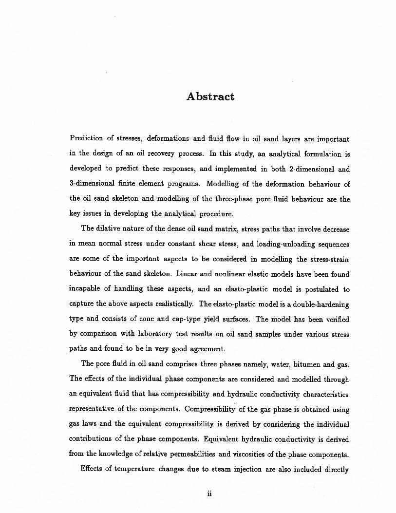
Abstract
Prediction of stresses, deformations and fluid flow in oil sand layers are important
in the design of an oil recovery process. In this study, an analytical formulation is
developed to predict these responses, and implemented in both 2-dimensional and
3-dimensional finite element programs. Modelling of the deformation behaviour of
the oil sand skeleton and modelling of the three-phase pore fluid behaviour are the
key issues in developing the analytical procedure.
The dilative nature of the dense oil sand matrix, stress paths that involve decrease
in mean normal stress under constant shear stress, and loading-unloading sequences
are some of the important aspects to be considered in modelling the stress-strain
behaviour of the sand skeleton. Linear and nonlinear elastic models have been found
incapable of handling these aspects, and an elasto-plastic model is postulated to
capture the above aspects realistically. The elasto-plastic model is a double-hardening
type and consists of cone and cap-type yield surfaces. The model has been verified
by comparison with laboratory test results on oil sand samples under various stress
paths and found to be in very good agreement.
The pore fluid in oil sand comprises three phases namely, water, bitumen and gas.
The effects of the individual phase components are considered and modelled through
an equivalent fluid that has compressibility and hydraulic conductivity characteristics
representative of the components. Compressibility of the gas phase is obtained using
gas laws and the equivalent compressibility is derived by considering the individual
contributions of the phase components. Equivalent hydraulic conductivity is derived
from the knowledge of relative permeabilities and viscosities of the phase components.
Effects of temperature changes due to steam injection are also included directly
11

in the stress-strain relation and in the flow continuity equations. The analytical
equations for the coupled stress, deformation and flow problem are solved by a finite
element procedure. The finite element programs have been verified by comparing the
program results with closed form solutions and laboratory test results.
The finite element program has been applied to predict the responses of a hor
izontal well pair in the underground test facility of Alberta Oil Sand Technology
and Research Authority (AOSTRA). The results are discussed and compared with
the measured responses wherever possible, and indicate the analysis gives insights
into the likely behaviour in terms of stresses, deformations and flow and would be
important in the successful design and operation of an oil recovery scheme.
111
Table of Contents
Abstract ii
List of Tables x
List of Figures xi
Acknowledgement xvi
Nomenclature xvii
1 Introduction 1
1.1 Characteristics of Oil Sand 4
1.2 Scope and Organization of the Thesis 8
2 Review of Literature 10
2.1 Stress-Strain Models 10
2.1.1 Stress-Strain Behaviour of Oil Sands 11
2.1.2 Stress-Strain Models for Sand 19
2.1.2.1 Elasto-Plastic Models 20
2.1.2.2 Constituents of Theory of Plasticity 22
2.1.3 Stress Dilatancy Relation 23
2.1.4 Modelling of Stress-Strain Behaviour of Oil Sand 24
2.2 Modelling of Fluid Flow in Oil Sand 25
2.3 Coupled Geomechanical-Fluid Flow Models for Oil Sands 27
2.4 Comments 30
iv
3 Stress-Strain Model Employed
3.1 Introduction
3.2 Description of the Model
3.3 Plastic Shear Strain by Cone-Type Yielding
3.3.1 Background of the Model
3.3.2 Yield and Failure Criteria
3.3.3 Flow Rule
3.3.4 Hardening Rule
3.3.5 Development of Constitutive Matrix [C8] .
3.4 Plastic Collapse Strain by Cap-Type Yielding
3.4.1 Background of the Model
3.4.2 Yield Criterion
3.4,3 Flow Rule
3.4.4 Hardening Rule
3.4.5 Development of Constitutive Matrix [Cc]
3.5 Elastic Strains by Hooke’s Law
3.6 Development of Full Elasto-Plastic Constitutive Matrix
3.7 2-Dimensional Formulation of Constitutive Matrix
3.8 Inclusion of Temperature Effects
3.9 Modelling of Strain Softening by Load Shedding
3.9.1 Load Shedding Technique
3.10 Discussion
4 Stress-Strain Model - Parameter Evaluation and
4.1 Introduction
4.2 Evaluation of Parameters
4.2.1 Elastic Parameters
4.2.1.1 Parameters kE and n
32
32
35
37
37
42
47
48
51
55
55
57
58
58
59
61
62
• 65
• 67
68
70
72
74
74
74
75
75
Validation
v

4.2.1.2 Parameters kB and m
Evaluation of Plastic Collapse Parameters
Evaluation of Plastic Shear Parameters
4.2.3.1 Evaluation of ij and L2
4.2.3.2 Evaluation of and )
4.2.3.3 Evaluation of KG, np and R1
4.2.4 Evaluation of Strain Softening Parameters
4.3 Validation of the Stress-Strain Model
4.3.1 Validation against Test Results on Ottawa Sand
4.3.1.1 Parameters for Ottawa Sand
4.3.1.2 Validation
4.3.2 Validation against Test Results on Oil Sand
4.3.2.1 Parameters for Oil Sand
4.3.2.2 Validation
4.4 Sensitivity Analyses of the Parameters
4.5 Summary
76
4.2.2
4.2.3
79
80
82
82
83
86
87
88
91
96
96
101
107
109
114
5 Flow Continuity Equation 115
5.1 Introduction 115
5.2 Derivation of Governing Flow Equation 116
5.3 Permeability of the Porous Medium 123
5.4 Evaluation of Relative Permeabilities 124
5.5 Viscosity of the Pore Fluid Components 132
5.5.1 Viscosity of Oil 132
5.5.2 Viscosity of Water 134
5.5.3 Viscosity of Gas 136
5.6 Compressibility of the Pore Fluid Components 136
5.7 Incorporation of Temperature Effects 140
vi

5.8 Discussion. 142
6 Analytical and Finite Element Formulation
6.1 Introduction
6.2 Analytical Formulation
6.2.1 Equilibrium Equation
6.2.2 Flow Continuity Equation
6.2.3 Boundary Conditions
6.3 Drained and Undrained Analyses
6.4 Finite Element Formulation
6.5 Finite Elements and the Procedure Adopted
6.5.1 Selection of Elements
6.5.2 Nonlinear Analysis
6.5.3 Solution Scheme
6.5.4 Finite Element Procedure
6.6 Finite Element Programs
6.6.1 2-Dimensional Program CONOIL-Il .
6.7 3-Dimensional Program CONOIL-Ill
7 Verification and Application of the Analytical Procedure
7.1 Introduction
7.2 Aspects Checked by Previous Researchers . .
7.3 Validation of Other Aspects
7.4 Verification of the 3-Dimensional Version
7.5 Application to an Oil Recovery Problem
7.5.1 Analysis with Reduced Permeability .
7.6 Other Applications in Geotechnical Engineering
144
144
145
146148148149152158
158
159
162
164
166
166
167
168
168168175181
183
203208
vii

8 Summary and Conclusions 216
8.1 Recommendations for Further Research 219
Bibliography 220
Appendices 242
A Load Shedding Formulation 242
A.1 Estimation of {LO}LS 243
A.2 Estimation of {F}Ls 245
B Relative Permeabilities and Viscosities 247
B.1 Calculations of relative permeabilities 247
B.1.1 Relevant equations . 247
B.1.2 Example data . . 249
B.1.3 Sample calculations . 249
B.2 Viscosity of water 250
B.3 Viscosity of hydrocarbon gases (from Carr et al., 1954) 252
B.3.1 Example calculation 254
C Subroutines in the Finite Element Codes 258
C.1 2-Dimensional Code CONOIL-Il 258
C.1.1 Geometry Program 258
C.1.2 Main Program 259
C.2 3-dimensional code CONOIL-Ill 261
D Amounts of Flow of Different Phases 264
E User Manual for CONOIL-Il 270
E.1 Introduction 270
E.2 Geometry Program 272
viii
E.3 Main Program.275
E.4 Detail Explanations 292
E.4.1 Geometry Program 292
E.4.2 Main Program 295
F User Manual for CONOIL-Ill 304
F.1 Introduction 304
F.2 Input Data 305
F.3 Example Problem 1 319
F.3.1 Data File for Example 1 320
F.3.2 Output file for Example 1 321
ix
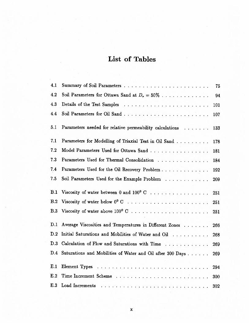
List of Tables
4.1 Summary of Soil Parameters 75
4.2 Soil Parameters for Ottawa Sand at Dr = 50% 94
4.3 Details of the Test Samples 101
4.4 Soil Parameters for Oil Sand 107
5.1 Parameters needed for relative permeability calculations 133
7.1 Parameters for Modelling of Triaxial Test in Oil Sand 178
7.2 Model Parameters Used for Ottawa Sand 181
7.3 Parameters Used for Thermal Consolidation 184
7.4 Parameters Used for the Oil Recovery Problem. . 192
7.5 Soil Parameters Used for the Example Problem 209
B.1 Viscosity of water between 0 and 1000 C 251
B.2 Viscosity of water below 00 C 251
B.3 Viscosity of water above 1000 C 251
D.1 Average Viscosities and Temperatures in Different Zones 266
D.2 Initial Saturations and Mobilities of Water and Oil 268
D.3 Calculation of Flow and Saturations with Time 269
D.4 Saturations and Mobilities of Water and Oil after 300 Days 269
E.1 Element Types 294
E.2 Time Increment Scheme 300
E.3 Load Increments 302
x

List of Figures
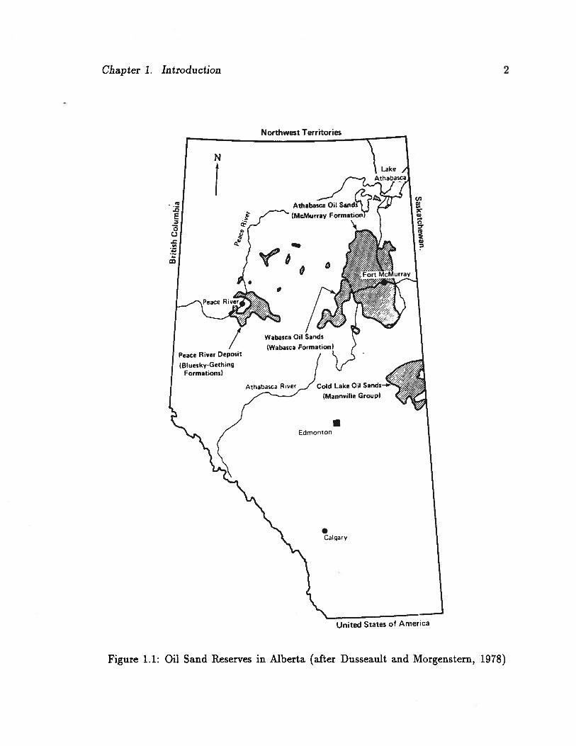
1.1 Oil Sand Reserves in Alberta (after Dusseault and Morgenstern, 1978) 2
1.2 In-situ Structure of Oil Sand (after Dusseault,1980) 6
1.3 Undrained Equilibrium behaviour of an Element of Soil upon Unload
ing (after Sobkowicz and Morgenstern, 1984) 7
2.1 Fabric of Granular Assemblies (after Dusseault and Morgenstetn, 1978) 12
2.2 Residual and Peak Shear Strengths of Athabasca Oil Sand (after Dusseault
and Morgenstern, 1978) 13
2.3 Effect of Stress Path on Stress-Strain Behaviour (after Agar et al., 1987) 14
2.4 Shear Strength of Athabasca Oil Sand and Ottawa Sand (after Agar
et al., 1987) 15
2.5 Effect of Temperature on Stress-Strain Behaviour (after Agar et al.,
1987) 16
2.6 Comparison of Athabasca and Cold Lake Oil Sands (after Kosar et al.,
1987) 18
3.1 A Possible Stress Path During Steam Injection 34
3.2 Components of Strain Increment 36
3.3 Mobilized Plane under 2-D Conditions 38
3.4 Spatial Mobilized Plane under 3-D Conditions 40
3.5 Yield and Failure Criteria on TSMp— °sMp Space . . 43
3.6 Matsuoka-Nakai and Mohr-Coulomb Failure Criteria 45
3.7 Effect of Intermediate Principal Stress (After Salgado (1990)) . . . 46
3
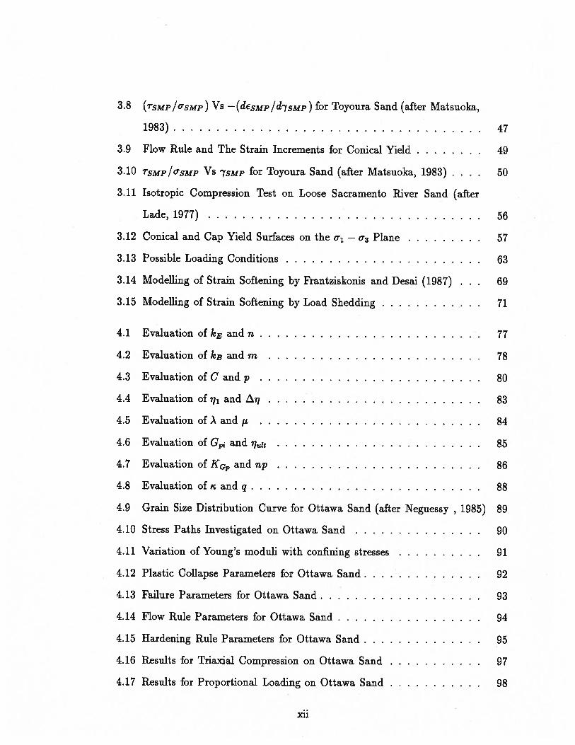
3.8 (TsMp /osMP) Vs — (desMp /d7sMp) for Toyoura Sand (after Matsuoka,
1983) 47
3.9 Flow Rule and The Strain Increments for Conical Yield 49
3.10 TSMp/o5Mp Vs YsMP for Toyoura Sand (after Matsuoka, 1983) . . . 50
3.11 Isotropic Compression Test on Loose Sacramento River Sand (after
Lade, 1977) 56
3.12 Conical and Cap Yield Surfaces on the o — o3 Plane 57
3.13 Possible Loading Conditions 63
3.14 Modelling of Strain Softening by Frantziskonis and Desai (1987) . . 69
3.15 Modelling of Strain Softening by Load Shedding 71
4.1 Evaluation of kE and ii 77
4.2 Evaluation of kB and m 78
4.3 Evaluation of C and p 80
4.4 Evaluation of and L 83
4.5 Evaluation of ) and it 84
4.6 Evaluation of G1, and ‘quit 85
4.7 Evaluation of K0 and np . 86
4.8 Evaluation of , and q 88
4.9 Grain Size Distribution Curve for Ottawa Sand (after Neguessy , 1985) 89
4.10 Stress Paths Investigated on Ottawa Sand 90
4.11 Variation of Young’s moduli with confining stresses 91
4.12 Plastic Collapse Parameters for Ottawa Sand 92
4.13 Failure Parameters for Ottawa Sand 93
4.14 Flow Rule Parameters for Ottawa Sand 94
4.15 Hardening Rule Parameters for Ottawa Sand 95
4.16 Results for Triaxial Compression on Ottawa Sand 97
4.17 Results for Proportional Loading on Ottawa Sand 98
xii

4.18 Results for Various Stress Paths on Ottawa Sand 99
4.19 Grain Size Distribution for Athabasca Oil Sands, (after Edmunds et
al., 1987) . . . 100
4.20 Determination of kB and m for Oil Sand 102
4.21 Plastic Collapse Parameters for Oil Sand 103
4.22 Failure Parameters for Oil Sand 104
4.23 Determination of and np for Oil Sand 105
4.24 Flow Rule Parameters for Oil Sand 106
4.25 Results for Isotropic Compression Test on Oil Sand 108
4.26 Results for Triaxial Compression Tests on Oil Sand 110
4.27 Results for Tests with Various Stress Paths on Oil Sand . . . 111
4.28 Sensitivity of Parameters C,p,A and p 112
4.29 Sensitivity of Parameters KG, np, R1 and i 113
5.1 One dimensional flow of a single phase in an element 117
5.2 Typical two-phase relative permeability variations (after Aziz and Set
tan, 1979) 125
5.3 Zone of mobile oil for three-phase flow (after Aziz and Settari, 1979) 127
5.4 Comparison of calculated and experimental three-phase oil relative per
meability (after Kokal and Maini, 1990) 130
5.5 Comparison of calculated and experimental relative permeabilities us
ing power law functions 131
5.6 Experimental and predicted values of viscosity (after Puttagunta et al.,
1988) 135
6.1 Finite Element Types Used in 2-Dimensional Analysis 160
6.2 Finite Element Types Used in 3-Dimensional Analysis 161
6.3 Flow Chart for the Finite Element Programs 165
xiii
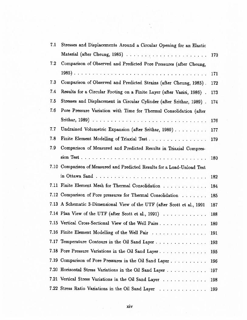
7.1 Stresses and Displacements Around a Circular Opening for an Elastic
Material (after Cheung, 1985) 170
7.2 Comparison of Observed and Predicted Pore Pressures (after Cheung,
1985) 171
7.3 Comparison of Observed and Predicted Strains (after Cheung, 1985) 172
7.4 Results for a Circular Footing on a Finite Layer (after Vaziri, 1986) 173
7.5 Stresses and Displacement in Circular Cylinder (after Srithar, 1989) 174
7.6 Pore Pressure Variation with Time for Thermal Consolidation (after
Srithar, 1989) 176
7.7 Undrained Volumetric Expansion (after Srithar, 1989) 177
7.8 Finite Element Modelling of Triaxial Test 179
7.9 Comparison of Measured and Predicted Results in Triaxial Compres
sion Test 180
7.10 Comparison of Measured and Predicted Results for a Load-Unload Test
in Ottawa Sand 182
7.11 Finite Element Mesh for Thermal Consolidation 184
7.12 Comparison of Pore pressures for Thermal Consolidation 185
7.13 A Schematic 3-Dimensional View of the UTF (after Scott et al., 1991 187
7.14 Plan View of the UTF (after Scott et al., 1991) 188
7.15 Vertical Cross-Sectional View of the Well Pairs 189
7.16 Finite Element Modelling of the Well Pair 191
7.17 Temperature Contours in the Oil Sand Layer 193
7.18 Pore Pressure Variations in the Oil Sand Layer 195
7.19 Comparison of Pore Pressures in the Oil Sand Layer 196
7.20 Horizontal Stress Variations in the Oil Sand Layer 197
7.21 Vertical Stress Variations in the Oil Sand Layer 198
7.22 Stress Ratio Variations in the Oil Sand Layer 199
xiv

7.23 Comparison of Horizontal Displacements at 7 m from Wells 200
7.24 Vertical Displacements at the Injection Well Level 201
7.25 Total Amount of Flow with Time 202
7.26 Individual Flow Rates of Water and Oil 204
7.27 Total Amount of Oil Flow 205
7.28 Pore Pressure Variation for Analysis 2 206
7.29 Stress Ratio Variation for Analysis 2 207
7.30 Details of the Cases Analyzed 210
7.31 Variation of Pore Pressure Ratio for Case 1 212
7.32 Variation of Pore Pressure Ratio for Case 2 213
7.33 Variation of Pore Pressure Ratio for Case 3 214
A.1 Strain Softening by Load Shedding 242
B.1 Prediction of pseudocritical properties from gas gravity . . 253
B.2 Viscosity of hydrocarbon gases at one atmosphere 254
B.3 Viscosity ratio vs pseudo-reduced pressure 255
B.4 Viscosity ratio vs pseudo-reduced temperature 256
D.1 Zones involved in Fluid Flow. . 265
E.1 Nodes along element edges . . 290
E.2 Element types 293
E.3 Plane Strain Condition 296
E.4 Axisymmetric Condition . . . 296
F.1 Available Element Types . . . 306
F.2 Finite element mesh for example problem 1 319
xv

Acknowledgement
The author is greatly indebted to his supervisor Professor P. M. Byrne for his guid
ance, valuable suggestions and the encouragement throughout this research.
The author wishes to express his appreciation to the members of the supervisory
committee for reviewing the manuscript and making constructive criticisms. Appre
ciation is also extended to Mr. Jim Grieg for his valuable helps on the computer
aspects.
The author expresses his gratitude to his wife, Vasuki, for her support and toler
ance of the odd working habits of a graduate student.
The author would like to thank his colleagues in Dept. of Civil Engineering , in
particular, Uthayakumar and Hendra for sharing common interest.
Finally, the fellowship awarded by the University of British Columbia and the
research grant provided by Alberta Oil Sand Technology and Research Authority
(AO STRA) are gratefully acknowledged.
xvi

Nomenclature
B bulk modulus
B pore pressure shape function derivatives
displacement shape function derivatives
C plastic collapse modulus
CEQ equivalent compressibility
D stress-strain matrix
E Young’s modulus
e void ratio
F body force vector
f plastic collapse yield function
initial plastic shear parameter
Gt tangent plastic shear parameter
H Henry’s constant
I, 12 and 13 stress invariants
K0 plastic shear number
k Darcy’s permeability of the porous medium
kB bulk modulus number
Young’s modulus number
kEQ equivalent hydraulic conductivity
kh permeability in horizontal direction
kmi mobility of phase ‘1’
kmT total mobility
xvii

kri relative permeability of phase ‘1’
krog relative permeability of oil in oil-gas system
kr relative permeability of oil in oil-water system
relative permeability of oil at critical water saturation
permeability in vertical direction
l, l, and l direction cosines of o to the x, y and z axes
M constrained modulus
m bulk modulus exponent
mz,my and m direction cosines of o-2 to the x, y and z axes
N shape functions for pore pressures
N shape functions for displacements
n Young’s modulus exponent
n, n, and n2 direction cosines of o3 to the x, y and z axes
np plastic shear exponent
P pore pressure
Pa atmospheric pressure
capillary pressure
p plastic collapse exponent
q strain softening exponent
failure ratio
S saturation
normalized saturation
residual oil saturation
S critical water saturation
t time
U displacement vector
V volume
xviii
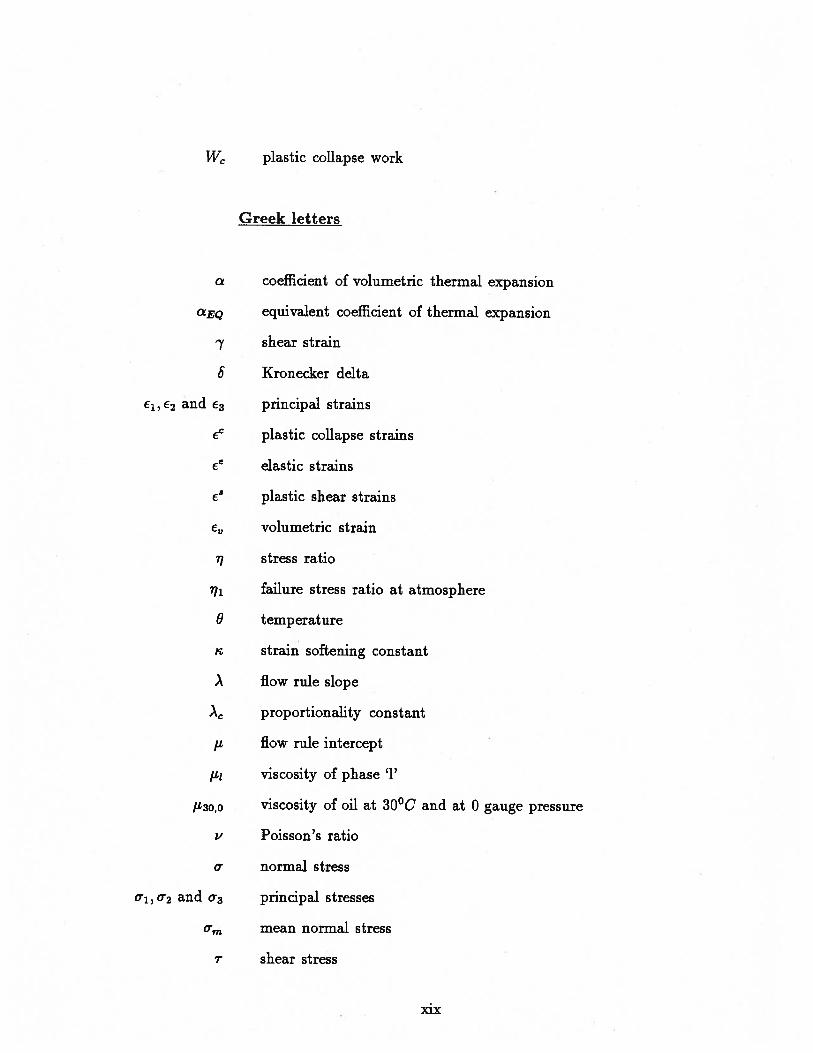
W plastic collapse work
Greek letters
coefficient of volumetric thermal expansion
cEQ equivalent coefficient of thermal expansion
shear strain
Kronecker delta
El, 62 and 63 principal strains
plastic collapse strains
6e elastic strains
plastic shear strains
volumetric strain
stress ratio
failure stress ratio at atmosphere
8 temperature
strain softening constant
flow rule slope
proportionality constant
p flow rule intercept
viscosity of phase ‘1’
P30,0 viscosity of oil at 30°C and at 0 gauge pressure
v Poisson’s ratio
normal stress
1, 2 and u3 principal stresses
mean normal stress
r shear stress
xix
(6m mobilized friction angle
Subscripts
f failure state
g gas phase
j partial derivative with respect to j
MP mobilized plane
o oil phase
SMP spatial mobilized plane
ult ultimate state
w water phase
Superscripts
c plastic collapse condition
e elastic condition
plastic shear condition
xx

Chapter 1
Introduction
The oil contained in oil sand deposits in northern Alberta is one of the major resources
in Canada. These deposits underlie an area of about 32,000 square kilometres with
estimated in-place reserves of 146.5 million cubic meters (Mosscop, 1980). Much of the
oil exists as high viscosity bitumen in Arenaceous Cretaceous formations, primarily in
the Athabasca oil sand deposits (see figure 1.1). Approximately 5% of these deposits
are found at depths less than 50 m and the rest are encountered at depths from 200
to 700 m.
Oil recovery schemes involve open pit mining in the shallow oil sand formations,
and in-situ extraction techniques such as tunnels and well-bores in the deep oil sand
formations. In the in-situ extraction procedures some form of heating is often required
as the very high viscosity of the bitumen makes conventional recovery by pumping
impractical. In-situ thermal methods such as steam injection through vertical well-
bore have been used and are relatively effective for the recovery of heavy oil from
deep seated formations. There have been, however, numerous well casing failures and
instability problems reported during field injection trials. During steam injection,
high pore fluid and stress gradients are created around the well-bore which can lead
to the instability and collapse of the well casing. Therefore, to understand the mech
anisms involved and to design these oil recovery schemes rationally and economically,
analyses which capture the complex engineering characteristics of the oil sand are
necessary.
Analyzing the problems related to oil sands is somewhat different from analyzing
1
Chapter 1. Introduction 2
United States of Amenca
Figure 1.1: Oil Sand Reserves in Alberta (after Dusseault and Morgenstern, 1978)
Northwest Territories
Chapter 1. Introduction 3
a general geotechnical problem because of the nature of the oil sand and the recovery
process involved. Oil sand comprises four phases; solid, water, bitumen and gas,
whereas, a general soil consists of three phases; solid, water and air. The presence of
bitumen and gas makes the analytical procedures for oil sands different and difficult.
Oil recovery by steam injection will cause changes in temperature and their effects
are also of prime concern. The changes in temperature induce changes in volume and
pore fluid pressure which in turn affect the engineering properties such as strength,
compressibility and hydraulic conductivity. When there is an increase in temperature,
if the volume change of the pore fluid components is greater than that of the voids
in the soil skeleton, there will be an increase in pore pressure and consequently a
reduction in effective stress. The effective stresses may become zero and liquefaction
may occur, if the oil sand is subjected to rapid increase in temperature and if an
undrained condition prevails.
The deformation and flow behaviour of oil sand is governed by several factors.
However, it can be categorized into two major constituents; the behaviour of pore
fluids and the behaviour of sand skeleton. An analytical model for the oil sand was
first developed by Harris and Sobkowicz (1977); It was later extended by Byrne
and Grigg (1980), Byrne and Janzen (1984) and Byrne and Vaziri (1986). However,
these analytical models consider a linear or nonlinear elastic behaviour for the sand
skeleton. Oil sand is very dense in its natural state and shows significant dilation
upon shear. The linear and nonlinear elastic models are not capable of modelling the
dilation effectively. Furthermore, steam injection and subsequent recovery will lead
to loading and unloading cycles and for realistic modeffing an elasto-plastic model
is necessary. In this study, a double hardening elasto-plastic model is postulated for
the sand skeleton based on the models by Nakai and Matsuoka (1983) and by Lade
(1977), and it is very effective in handling the dilation.
With regard to the pore fluid behaviour, Byrne and Vaziri (1986) considered the
Chapter 1. Introduction 4
individual contributions of the pore fluid components in the compressibility but not in
the hydraulic conductivity. In this research work, the relative permeabilities of water,
bitumen and gas are considered and an equivalent hydraulic conductivity is derived
to model the pore fluid behaviour appropriately. The equivalent compressibility term
as proposed by Byrne and Vaziri (1986) is also included.
The effects of temperature changes in stresses and volume changes have been di
rectly included in the governing equilibrium and flow continuity equations. It should
be noted that the equation of thermal energy balance is not considered in the analyt
ical model. However, the temperature-time history which is obtained from a separate
heat flow analysis or by some other means is considered as an input to the analytical
model and, the effects of these temperature changes on the stress-strain behaviour
and the fluid flow are evaluated.
An analytical procedure considering all these aspects has been developed and
incorporated in the 2-dimensional finite element code CONOIL-Il. In order to analyze
the three dimensional effects a new 3-dimensional finite element code CONOIL-Ill is
also developed.
1.1 Characteristics of Oil Sand
Since the oil sand is different form a general soil, it is appropriate to present some
brief descriptions about its unusual characteristics. Oil sand can be considered as a
four phase geological material comprising solid, water, bitumen and gas. The two
dominant physical characteristics of the oil sand are the quartz mineralogy and the
large quantity of interstitial bitumen. The quartz grains of the oil sand are 99% water
wet as the water phase forms a continuous film around it. A larger portion of the
pore space is filled with bitumen and since bitumen and water form continuous phases,
gas can only exists in the form of discrete bubbles (free gas). However, significant
quantities of gas can also exist in the dissolved state in the pore fluid. An illustration
Chapter 1. Introduction 5
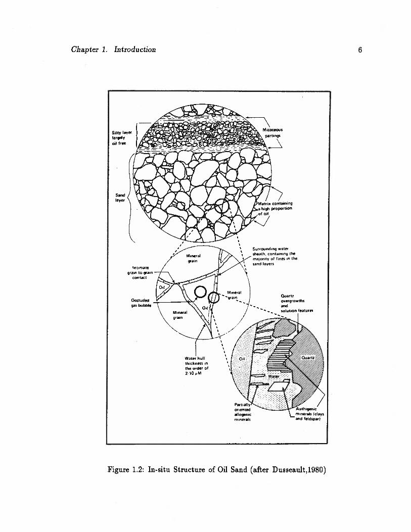
of oil sand structure (Dusseault, 1980) is shown in figure 1.2.
In its natural state, oil sand is very dense, uncemented, fine to medium grained
and exhibits high shear strength and dilatancy. It shows low compressibility charac
teristics compared to normal dense sand of similar mineralogy. The extremely high
viscosity of bitumen makes the effective hydraulic conductivity very low and causes
the oil sand to behave in an undrained manner.
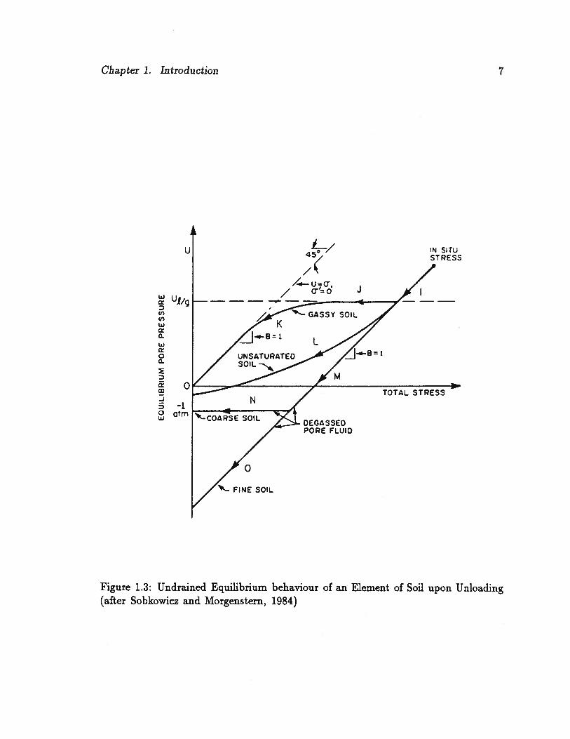
Another unusual characteristic of oil sand is its behaviour upon unloading. Be
cause of the very low effective hydraulic conductivity, oil sand behaves in an undrained
manner, however, it responds quite differently compared to the undrained behaviour
of a normal sand. Above the liquid-gas saturation pressure (U119), oil sand behaves
like a normal sand (path I of figure 1.3). A decrease in confining stress will result in a
decrease in pore pressure and the effective stress remains constant. When the level of
confining stress decreases below the liquid-gas saturation pressure, the dissolved gas
in the pore fluid comes out of solution and causes the pore fluid to become very com
pressible. At this point, the soil matrix commences to take the load and the effective
stress decreases while the pore pressure stays constant (path J). As the effective stress
decreases, the soil skeleton compressibility increases and becomes comparable to the
pore fluid compressibility. Then, the pore fluid takes the load and the pore pressure
starts to decrease again (path K). At some stage, the effective stress becomes zero
and the physical consequences of this process are significant increase in volume and
a marked reduction in shear strength. Plots of pore pressure versus total stress for
saturated (path M), unsaturated (path L) and gassy soils (path J-K) are shown in
figure 1.3. A comprehensive study of the gas exsolution phenomenon upon unloading
can be found in Sobkowicz and Morgenstern (1984).
Tj
I-.
(b I-.
U) I
I-.
0
CC
CC
--
m
rcn
oa;
-’ -C
—m
0o
m
-
a
C
-
,oo a..
C-
Chapter 1. Introduction 7
U
Uj/gD(I,C,,w0
LAJ
00
I ..°
atm
Figure 1.3: Undrained Equilibrium behaviour of an Element of Soil upon Unloading(after Sobkowicz and Morgenstern, 1984)
//..—. u=o,
____,_,_
o-c=o J
IN SITUSTRESS
/
TOTAL STRESS
CEGASSEDPORE FLUID
0
FINE SOIL

Chapter 1. Introduction 8
1.2 Scope and Organization of the Thesis
The objective of this study is to present a better analytical formulation for the stress,
deformation and flow analysis in oil sands, from a geotechnical point of view. The
analytical model is developed on the premise that the oil sand is a four phase material
comprising solid, water, bitumen and gas.
In developing the analytical formulation the key issues are; a stress-strain model
for the sand skeleton, the compressibility and permeability characteristics of the three-
phase pore fluid, the effects of temperature, and the overall analytical and finite
element procedure. Discussions on these issues highlighting the previous research
works in the literature are given in chapter 2.
The main feature in a deformation analysis is the stress-strain model employed. In
this study, a double-hardening elasto-plastic model is postulated. The fundamental
details of the stress-strain model and the development of the constitutive matrix
using plastic theories are described in chapter 3. The parameters required for the
stress-strain model, procedures to obtain them, the sensitivity of these parameters
and the verification of the stress-strain model against laboratory results are presented
in chapter 4.
One of the major concerns in the analytical formulation presented in this study
is the modelling of the multi-phase fluid. Chapter 5 describes the development of the
flow continuity equation, considering the contributions from all the fluid phase com
ponents, in detail. Inclusion of temperature effects in the flow continuity equation is
also given in this chapter. Inclusion of the temperature effects in stress-strain relation
is explained in chapter 3. Details concerning the overall analytical procedure and its
implementations in 2-dimensional and 3-dimensional finite element formulations are
given in chapter 6.
Verifications and the validations of the developed formulation are presented in
chapter 7. Some specific problems where closed form solutions are available and some

Chapter 1. Introduction 9
laboratory experiments are considered and the results are compared. Application to
an oil recovery process by steam injection is presented and the results are analyzed
in detail. Possible applications of the developed formulation for general geotechnical
problems are discussed and an example problem is also given.
Chapter 8 summarizes the important findings of this research work. Some com
ments on the aspects which warrant further investigation are also stated in this chap
ter.
Chapter 2
Review of Literature
The research work carried out in this study can be broadly classified under the fol
lowing topics; stress-strain model for the oil sand, modelling of flow characteristics of
the three-phase pore fluid; and the analytical and finite element formulations. There
fore, it is appropriate to present a review on the previous research works under these
subheadings. The intention of the literature review presented in this chapter is not
to critically assess each and every research work but to give an overall picture, and
to set the stage to discuss the work carried out in this study.
2.1 Stress-Strain Models
The stress-strain behaviour of the oil sand skeleton is essentially the stress-strain
behaviour of a dense sand. This conclusion was not widely accepted until the com
pletion of series of research programs at the University of Alberta in the late 1970s
and in 1980s. In particular, the perception of bitumen as a cementing material was
widely held until the last decade, as many geologists and petroleum engineers failed
to recognize the geomechanical behaviour of the sand skeleton. It is now recognized
that the oil sands must be considered as a particulate material and its behaviour can
be described by an appropriate stress-strain model. Before going into a detailed re
view of the stress-strain models, it will be useful to describe the observed stress-strain
behaviour of oil sands. The next subsection summarizes the stress-strain behaviour
of oil sands in laboratory experiments.
10
Chapter 2. Review of Literature 11
2.1.1 Stress-Strain Behaviour of Oil Sands
Dusseault (1977) showed that the Athabasca oil sands have an extremely stiff struc
ture in the undisturbed state, accompanied by a large degree of dilation when loaded
to failure and subsequent yield. This was attributed to its extreme compactness which
provides extensive grain-to-grain contact. The grain orientations of the oil sand are
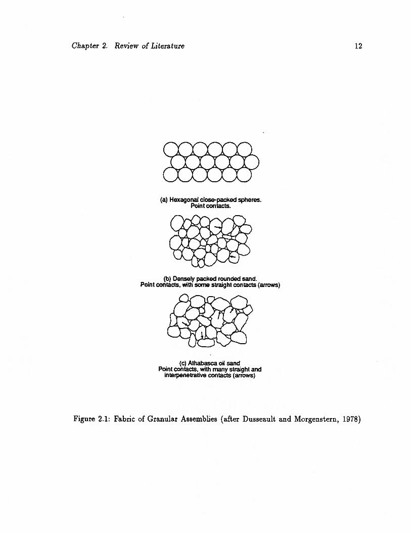
compared schematically to ideal and rounded sand grains in figure 2.1. The angular
ity of the Athabasca sand grains illustrate why significant dilation can be expected
as the sand is sheared.
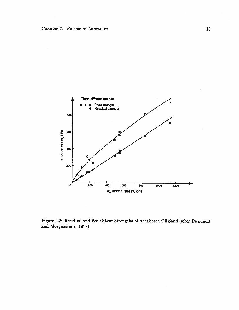
Dusseault and Morgenstern (1978) studied the shear strength of Athabasca oil
sands and stated that the Mohr-Coloumb failure envelope is not a straight line but
curvilinear. The residual and peak shear strengths measured in direct shear tests are
shown in figure 2.2. The curvilinear nature is said to be due to the dilatancy and the
grain surface asperity.
Agar et al. (1987) carried out extensive testing on Athabasca oil sand to study the
effects of temperature, pressure and stress paths on shear strength and stress-strain
behaviour. Figure 2.3 shows the effect of stress paths on stress-strain behaviour.
Six different triaxial stress paths were investigated which are shown in figure 2.3(a).
Typical stress-strain curves for these stress paths are plotted in figure 2.3(b). These
curves illustrate the influence of stress paths on peak deviator stress and stress-strain
behaviour. It can be seen from the figure that the dilatancy is more pronounced on
certain stress paths (see paths B and C), and at lower effective confining stress than
at higher stress levels (compare paths C and D).
Figure 2.4 shows the shear strength of Athabasca oil sand compared to dense
Ottawa sand. The shear strength of oil sand is greater than that of dense Ottawa
sand at lower effective confining stress levels. However, at higher stress levels, the
strengths of these two materials apparently converge.
Figure 2.5 shows the effect of temperature for a drained triaxial compression test.
Chapter 2. Review of Literature 12
(a) Hexagonal close-packed spheres.Point contacts.
(b) Densely packed rounded sand.Point contacts, with some straight contacts (arrows)
(c) Athabasca oil sandPoint contacts, with many straight and
interpenetrative contacts (arrows)
Figure 2.1: Fabric of Granular Assemblies (after Dusseault and Morgenstern, 1978)
Chapter 2. Review of Literature 13
a.
U,0
L0
(U0-c(0
Figure 2.2: Residual and Peak Shear Strengths of Athabasca Oil Sand (after Dusseaultand Morgenstern, 1978)
Three different samples
o o Peak strength• Residual strength
•
0 200 400 600 800
o normal stress, kPa
1000 1200

(a) Various Stress Paths
b
>0
(b) Stress-Strain Behaviour
Figure 2.3: Effect of Stress Path on Stress-Strain Behaviour (after Agar et al., 1987)
I;
Chapter 2. Review of Literature 14
28
24
20
16
a
20
16
12
8
4
00.5
12
0 4 8 12
./7O1 (MPa)
16—0.5
0.5 1.0 1.5
e (%)

Chapter 2. Review of Literature 15
60
a)
aUCDU,
ina,40
U)CI
U
-C‘/,— 300a)U)C
20
Figure 2.4: Shear Strength of Athabasca Oil Sand and Ottawa Sand (after Agar etal., 1987)
. LEGEND
D
.Athobasca Oil Sand v
ATHABASCA OIL SAND (This Study)OTTAWA SAND (This StudyDIJSSEAUT & MORGENSTERN(1978)SOBKOWICZ (1982)DUNCAN & CHANG (1970)
.
1 2 3 4 5 6 7 8
Effective Confining Stress c (MPa)

Chapter 2. Review of Literature 16
The effect of temperature on the stress-strain behaviour does not seem to be signifi
cant. For some other stress paths, it appeared that the temperature has considerable
influence on the stress-strain behaviour. However, Agar et al (1987). concluded that
the differences in the stress-strain behaviour at various temperatures are small. They
attributed the observed differences to the disturbances in sampling and the mate
rial heterogeneities. The test results appeared to be far more sensitive to sample
disturbances than heating.
0 0.5 1.0
e (%)
Figure 2.5: Effect of Temperature on Stress-Strain Behaviour (after Agar et al., 1987)
Kosar (1989) continued Agar’s work and tested various oil sands and noted some
essential differences in the geomechanical behaviour. Kosar claimed that in addition
20
16
12
4
0
04
1.5 2.0
Chapter 2. Review of Literature 17
to temperature, pressure and stress paths, the grain mineralogy, geological environ
ment of deposition and the geological history are the major factors affecting the
geomechanical behaviour. The maximum shear strength and the stress-strain moduli
of Athabasca oil sands are much greater than those of Cold Lake oil sand reflecting
the grain mineralogy and the geological factors. Athabasca oil sands consist of a
uniformly graded, predominantly quartz sand, whereas, Cold Lake oil sands contain
several additional minerals which are weaker. Figure 2.6 shows typical drained tn-
axial compression test of these two oil sands. Athabasca oil sand exhibits dilatant
behaviour but the Cold Lake oil sand does not. In the Athabasca oil sand, the increase
in volume change during shear is also accompanied by strain softening behaviour in
the post peak region. The Cold Lake oil sand shows contractive behaviour and the
reason for this is the presence of weaker minerals. The weaker minerals are prone
to grain crushing at the applied stress levels. Because of these weaker minerals, the
geomechanical behaviour of Cold Lake oil sand changes with temperature as well.
Athabasca oil sands, on the other hand, do not show significant changes in behaviour
at different temperatures.
Wong et al. (1993) pointed out that testing of oil sand samples should include
some important stress paths which are expected to be encountered in the field. They
carried out detailed testing on Cold Lake oil sand which includes stress paths with
increasing and decreasing pore pressures under constant total stress. This results in
load-unload-reload stress paths in terms of effective stress ratio. They identified four
different modes of granular interactions namely; contact elastic deformation, shear
dilation, rolling and grain crushing for the observed geomechanical behaviour. They
also noticed grain crushing in Cold Lake oil sand when the effective confining stress
increased above 8 MPa.

Chapter 2. Review of Literature 18
6-
Mairjmshearsfl-ength = 16.9 MPa
5.I
a—4.OUPa
4 / Athabasca (Agar. 1984)
0
3• : Mi,m shaer strength • 6.9 MPa
I2. :
Athabasca £ - 2200 MPa
‘7 CoidLake
S
Axial Strain (%)
Figure 2.6: Comparison of Athabasca and Cold Lake Oil Sands (after Kosar et aL,1987)

Chapter 2. Review of Literature i9
Therefore, the modelling of oil sand behaviour should include two significant fea
tures; non-recoverable strains and dilatancy. A realistic model must take the deforma
tion history into account, particularly if the stresses are to be cycled through loading
and unloading. The elasto-plastic formulation incorporates these features naturally.
There are a number of elasto-plastic stress-strain models available for sands in the
literature and a brief review of those are presented next.
2.1.2 Stress-Strain Models for Sand
A number of models have been proposed in the literature for the stress-strain be
haviour of sand. Most of them make use of the well developed classical theories of
elasticity and plasticity either separately or in a combined form. These theories are
based on the observations made on materials that can be described in the context of
continuum mechanics. To adopt these theories to model the stress-strain behaviour
of sand, they have to be modified. Different modifications are made to capture dis
tinguished features of sand behaviour and thus, different models are proposed by
different researchers. One of the difficult features of sand behaviour to model has
been the shear induced volume change.
Basically, constitutive models can be classified into two categories; linear or in
cremental elastic models and elasto-plastic models. In the theory of elasticity, the
state of stress is uniquely determined by the state of strain so that the stress-strain
response of an elastic models is independent of the stress path. The simplest elastic
model would be the isotropic linear elastic model which requires only two material
parameters. Incremental elastic models (Duncan and Chang (1970), Duncan et al.
(1980)) are the most commonly used because they can capture the nonlinearity and
are easy to use. Essentially, the incremental elastic models also require only two pa
rameters when analyzing a load increment. However, to update these two material
parameters with stress levels and to model the nonlinearity additional parameters are

Chapter 2. Review of Literature 20
necessary. Generally, in elastic models, the shear and normal stresses and strains are
uncoupled from each other. Byrne and Eldrige (1982) incorporated the shear volume
coupling effects in the incremental elastic models using a stress dilatancy equation.
Reviews of the existing elastic and elasto-plastic constitutive models are avail
able in the literature as state-of-the-art papers, special workshops and international
symposia. Ko and Sture (1980) provided a clear summary of the most important
models as of 1980 and described the methods needed to obtain their coefficients.
Chen (1982) described and analyzed what is meant by different levels of elasticity.
He also described some of the elasto-plastic models most commonly used for soils.
Scott (1985) presented a very lucid treatise on plasticity and stress-strain relations.
A series of workshops held at McGill University (1980), University of Grenoble (1982)
and Case Western University (1987) and the international symposia (ASCE sympo
sium, Florida, 1980; International Symposium, Deift, 1982) provide better insights
into the different stress-strain models.
Since an elasto-plastic model is proposed in this study, a brief review of elasto
plastic models and the related theories are presented next.
2.1.2.1 Elasto-Plastic Models
The theory of plasticity has been developed on the basis of observed stress-strain
behaviour of metals. Since soils exhibit plastic non-recoverable strains, the theory
of plasticity provides an attractive theoretical framework for the representation of
the stress-strain behaviour of soils. However, there are major differences such as the
presence of voids and the tendency for volume change during shear that distinguish
soils from metals (Lade, 1987).
In the elasto-plastic models, the strain increment is decomposed into an elastic
component and a plastic component. The amounts of elastic and plastic strains will
vary with the level of loading and unloading. The elastic strain increment is obtained
Chapter 2. Review of Literature 21
using the theory of elasticity and the plastic strain increment is obtained from the
theory of plasticity.
Drucker et al. (1955) were the first to treat soils as work hardening materials.
The yield surface that they postulated consists of a Mohr-Coloumb surface and a cap
which passes through the isotropic compression axis. Most of the elasto-plastic models
evolved from this study. The Cam-Clay model (Roscoe et al., 1958) introduced the
concept of critical state and presented an equation for the yield surface considering
energy dissipation. Prevost and beg (1975) used the critical state line concept in
their model, but defined two yield surfaces, one for volumetric and shear deformation
and the other for shear deformation alone. The Cam-Clay model has been used in
one form or another by many researchers, for example, Adachi and Okamo (1974),
Pender (1977), Nova and Wood (1979) and Wilde (1979).
The models of Lade and Duncan (1975) and Matsuoka (1974) contain features of
the Mohr-Coloumb criterion and incorporate the influence of intermediate principal
stress. The yield and failure surfaces are assumed to be described by similar functions
so that both surfaces have similar shapes. Lade (1977) introduced a yielding cap in
order to control the plastic volumetric strain making his model a double hardening
one. Vermeer (1978) also used a double hardening model. He divided the plastic
strain into two parts; one is described by means of a shear surface and the shear
dilatancy equation and the other is strictly volumetric.
Multiple yield surface plasticity theory has also been used to predict soil behaviour
(Iwan(1967), Prevost (1978, 1979)). In computations, this theory requires that the
positions, sizes and plastic moduli of each of the yield surfaces be stored for every
integration point, which is very tedious and therefore not very commonly used.
Chapter 2. Review of Literature 22
2.1.2.2 Constituents of Theory of Plasticity
In the theory of plasticity, existence of a yield function, a potential function and
a hardening function are necessary to relate the plastic strain increments to stress
increments mathematically. The yield function defines the stress conditions causing
plastic strains. The yield surface represented by the yield function encloses a volume
in the stress space, inside of which the strains are fully recoverable. Only stress
increments directed outward form the yield surface cause plastic strains. A stress
increment directed outward from the yield surface causes an expansion or translation
of the yield surface. During yielding, the state of stress remains on the yield surface
which is known as the consistency condition. A state of stress outside the yield surface
is not possible.
The direction of plastic strain increment is defined by the potential function which
is referred to as flow rule. If the potential function and the yield function are the
same, the flow rule is said to be associative. If these functions are different, then the
flow rule is non-associative.
The amplitude of the plastic strain increment is specified by the hardening func
tion. In plasticity, two types of hardening have been distinguished; isotropic hardening
and kinematic hardening. In a model undergoing isotropic hardening, the yield sur
face expands radially about the fixed axes. When the yield surface translates without
changing its size, the model undergoes kinematic hardening.
Once the constituents of the theory of plasticity are defined, the plastic strain
increment, can be calculated from,
=— n (2.1)
where,
Lo- - applied stress increment
n, - vector defining the unit normal to yield surface at the stress point
Chapter 2. Review of Literature 23
- vector defining the unit normal to potential surface at the stress point
H - plastic resistance
2.1.3 Stress Dilatancy Relation
The stress dilatancy theory derived from theoretical considerations has been used
extensively in stress-strain modeffing of sand. The stress dilatancy theory proposed
by Rowe (1962,1971) can be considered a remarkable effort to explain the shear de
formation behaviour. After Rowe, a number of other researchers published theories
to model the dilatancy following different approaches (Murayama (1964), Matsuoka
(1974), Oda and Konishi (1974), Nemat-Nasser (1980)). A noticeable difference be
tween Rowe’s theory and the other theories is that Rowe’s theory is independent of
the spatial distribution of interparticle contacts. Rowe’s theory considers that sliding
occurs on certain favourably oriented contact planes. The orientation of the sliding
planes will be such as to minimize the rate of dissipation of energy in sliding friction
between particles with respect to energy supplied.
Matsuoka (1974) developed the stress dilatancy relationship through a microscopic
point of view. He carried out shear tests by using cylindrical rods to model the
shearing mechanism of soil particles. From the fundamental measurements of the
angle of the interparticle contact, interparticle force and the angle of interparticle
friction, he developed a relationship between the shear resistance and the dilatancy.
Lade’s (1977) model incorporates the dilatancy through a empirical relation ob
tained by curve fitting. The equation relates a dilation parameter to the amount of
plastic work.
Nemat-Nasser (1980) presented an equation to describe the volumetric behaviour
of soil upon shearing which is based on the mechanics of the relative motion of the
grains at the micro level. The equation was obtained by considering the rate of
frictional losses and the energy balance.
Chapter 2. Review of Literature 24
2.1.4 Modelling of Stress-Strain Behaviour of Oil Sand
Modelling of the geomechanical behaviour of oil sand along with the pore fluid be
haviour, so as to describe gas exsolution and other related aspects was first presented
by Harris and Sobkowicz (1977). They considered a linear elastic model for the sand
skeleton behaviour.
A nonlinear elastic model with shear dilation was proposed by Byrne and Grigg
in 1980 to model the oil sand skeleton behaviour. Their model is based upon an
equivalent elastic analysis using a secant modulus and a single step loading. This was
subsequently extended by Byrne and Janzen (1984) who used an incremental tangent
modulus rather than a secant modulus. Vaziri (1986) basically used the same model
as Byrne and Janzen to represent the stress-strain behaviour of oil sand.
In the above cited references, the dilative behaviour of the material is incorporated
through a procedure borrowed from thermoelasticity. This method involves applying
equivalent nodal loads to predict the correct volume changes. Srithar et al. (1990)
pointed out that the thermoelastic approach encounters shortcomings specially in a
consolidation type of analysis. It predicts unrealistic oscillating results when large
time steps are considered. Furthermore, the computer algorithm necessitates two
levels of iterations; one for stress calculations, and the other for shear induced volume
change corrections. Wan et al. (1991) stated that the method of including dilation
through thermoelastic approach may lead to a decrease in effective mean normal stress
0m while in a pressuremeter test, dilation is always accompanied by an increase in
Tortike (1991) stated that cyclic steam simulation imposes cyclic loads on the oil
reservoir. He further suggested that a realistic stress-strain model should have the
capability to model the loading and unloading behaviour. He adopted Hinton and
Owen’s (1977) elasto-plastic model which includes a Mohr-Coloumb failure envelope
and an associated flow rule.
Chapter 2. Review of Literature 25
Wan et al. (1991) also recognized the cyclic loadings caused in the recovery
process by steam injection and proposed an elasto-plastic model for oil sand. Their
model is based on Vermeer’s (1982) elasto-plastic model. They used Matsuoka and
Nakai (1982) equation to represent the yield and failure surfaces, and a Ramberg
Osgood type hardening function. The model involves a non-associated flow rule and
the potential function is based upon Rowe’s stress dilatancy equation. However,
their model cannot predict the plastic volumetric behaviour for stress paths involving
compression with constant stress ratio.
2.2 Modelling of Fluid Flow in Oil Sand
In petroleum reservoir engineering, multiphase fluid flow has been analyzed by a
number of researchers without consideration of the geomechanical behaviour of the
oil sand matrix. The first clear attempt to use a finite element method for fluid
flow in porous medium that appeared in petroleum engineering was by Javandel and
Witherspoon (1968). They considered a single phase isothermal fluid flow through
an isotropic homogeneous porous medium. The numerical solutions were compared
with the analytical solutions for infinite, bounded and layered radial systems with
constant flow rate or pressure constraints and were found to be in good agreement.
Solutions for two-phase isothermal fluid flow problems using variational and finite
element methods were presented by various researchers (for example: Settari and
Price, 1976; Huyakorn and Pinder, 1977a; Spivak et al., 1977; Settari et al., 1977;
Lewis et al., 1978; White et al., 1981). Spivak et al. (1977) presented a formulation
for multi-dimensional, two-phase, immiscible flow using variational method. They
compared variational and finite difference methods and concluded that the variational
method is more efficient than the finite difference method. Galerkin’s procedure was
successfully applied to the analytical formulation of the governing equations in the
presence of favourable and unfavourable mobility ratios. Numerical dispersion at the
Chapter 2. Review of Literature 26
front was less in both cases than with the finite difference method. Also, in the
variational method, grid orientation effects were not observed.
Guibrandsen and Wile (1985) used Galerkin’s scheme directly for two-dimensional,
two-phase flow. The Newton-Raphson method was used to linearize the weighted
form, which was approximated in time by backward Euler differences. The spatial
domain was divided into rectangles and approximated by byliner functions. A sharper
front was noticed when the capillary pressure was not simply a constant function of
saturation, but oscillations in the solution still occurred downstream in the front.
However, no serious solution instability occurred.
Ewing (1989) proposed a mixed element scheme for solving pressure and velocity
in miscible and immiscible two-phase reservoir flow problems. Velocity was chosen
as the primary variable to ensure that it remains a smooth function throughout the
domain, despite step changes in reservoir properties governing the flow.
Faust and Mercer (1976), Huyakorn and Pinder (1977b), Voss(1978) and Lewis et
al. (1985) are some of the researchers who analyzed two-phase fluid flow under non-
isothermal conditions. Lewis et al. (1985) used the Galerkin method to solve the water
flow and energy equations in two dimensions. Byliner elements were used to model
hot water flooding for thermal oil recovery. Linear and higher order elements were
used to model the heat losses from the reservoir in all directions. Artificial diffusion
was introduced along streamlines to negate any grid orientations. The solutions were
found efficiently at the end of each time step using an alternating direct solution
algorithm.
The solution for multiphase fluid flow problem using finite elements was first pre
sented by McMichael and Thomas (1973). They analyzed a three-phase isothermal
flow in a two dimensional domain subdivided into linear finite elements. Reportedly,
no difficulties were encountered in finding the solution at each time step. The evalua
tion of all the reservoir properties at each quadrature point for numerical integration

Chapter 2. Review of Literature 27
appeared to obviate the need for upstream weighting for numerical stability. However,
this result is not in accordance with later studies of the multiphase flow problem by
the finite element method.
Tortike (1991) presented a detailed literature review on modelling of fluid flow
under isothermal and non-isothermal conditions. He solved the three-phase ther
mal flow problem using finite differences. He also tried to develop a fully coupled
geomechanical fluid flow model, but was not successful as the results were unstable.
It appears that in most of the research work in petroleum engineering, the flow
in oil sand is modelled by two phase system (water and bitumen) with reasonable
accuracy. However, these models solve only the fluid flow problem and do not con
sider the geomechanical behaviour. Therefore, the effects of stress distribution and
deformation in the oil sand matrix are not included in these models.
2.3 Coupled Geomechanical-Fluid Flow Models for Oil Sands
Some models in petroleum reservoir engineering include the effects of deformations
in oil sand matrix through poroelasticity. Geertsma (1957) combined the approaches
of Biot (1941) and Gassman (1951) to develop the equations of poroelasticity in a
more straightforward manner. He clearly defined and related the rock bulk and pore
compressibilities, and described the boundary conditions and procedure to determine
the correct parameters defining the compressibilities. Geertsma (1966) reviewed the
applications of poroelasticity in petroleum engineering. An analogy is presented be
tween poroelastic and thermoelastic theories, to take advantage of the many solutions
under different boundary conditions that have already been published. The concept
of the nucleus of strain for volume elements was described and it has been applied
to predict surface displacements. It should be noted however, the poroelastic theory
does not consider the effect of stress distribution through a porous medium.
Raghavan (1972) derived a one dimensional consolidation equation coupled with

Chapter 2. Review of Literature 28
fluid flow and compared his results with Terzhaghi’s solution. The general solution
was obtained from the partial differential equations describing the flow of fluid and
material displacement using a transform to convert it to an ordinary differential equa
tion. He also presented a significant review of the literature to that time.
Finol and Farouq Ali (1975) analyzed a two-phase flow model using finite differ
ences which included the effects of compaction on fluid flow and the prediction of
surface displacements. The problem was formulated by two discretized equations for
oil and water flow, and one analytical equation for poroelasticity which was numer
ically integrated. The variation of permeability and porosity was considered in the
analysis as the effect of compaction on ultimate recoveries. The authors concluded
that the ultimate recoveries of oil increased with compaction.
Harris and Sobkowicz (1977) derived an analytical model from a more geotechni
cal point of view. They presented a coupled mathematical model for the fluid flow
and the geomechanical behaviour of oil sand. The model was developed mainly to
analyze excavations, immediate foundation settlements and underground openings in
oil sands. Since these scenarios involve short term conditions, and because of the
high viscosity of the bitumen, their model was only concerned with the undrained
response. The authors claimed that the short term conditions govern the design in
the above circumstances.
Byrne and Grigg (1980), and Byrne and Janzen (1984) extended Harris and
Sobkowicz’s formulation. Byrne and Janzen also included the fully drained condition
in their analysis. Their analysis procedure involved an effective stress approach in
which the stresses in the sand skeleton were computed using a finite element scheme.
The pore fluid pressures were computed from the gas laws together with volume
compatibility between fluid and skeleton phases.
Vaziri (1986) coupled the equilibrium equation and the flow continuity equation
and analyzed the transient conditions as a consolidation problem. He included the

Chapter 2. Review of Literature 29
thermal effects on stresses, hydraulic conductivity and volume change and presented
a two dimensional finite element formulation. The fluid flow was considered as a
single phase one. The effects of different phase components on compressibility were
taken into account by means of an equivalent compressibility. Vaziri followed the
thermoelastic approach to model temperature effects. This approach appeared to
predict unrealistic oscillating results. Srithar (1989) incorporated the temperature
induced stresses and volume changes directly in the governing equilibrium and flow
continuity equations and presented a better formulation of Vaziri’s model.
Dusseault and Rothenberg (1988) reviewed the effect of thermal loading and pore
pressure changes around a wellbore on dilation and permeability. They described
the physical process of deformation in terms of particulate media. They concluded
that effective water permeability would increase one or two orders of magnitude with
dilation as the thickness of the water film coating the grains would increase by a
factor of two. The authors continue to document the changes likely from shear failure,
including the localization of shear and the growth of the shear zone from the edge of
a hydraulic fracture due to the altered stress state and the increased pore pressures.
Settari (1988), Settari et al. (1989) described a model to quantify the leak-off
rates for fracture faces in oil sand. The authors used a nonlinear elastic model and a
two-phase isothermal flow in their analysis. The nonlinear response was shown to give
a different pressure distribution than the linear elastic one. Settari (1989) extended
their earlier model to thermal flow.
Fung (1990) described a control volume finite element approach for coupled isother
mal two-phase fluid flow and solid behaviour. He adopted a hyperbolic stress-strain
law with Rowe’s stress dilatancy theory.
Chapter 2. Review of Literature 30
Schrefler and Simoni (1991) presented the equations for two-phase flow in a de
forming porous medium, which are, a linear momentum balance for the whole mul
tiphase system and continuity equations for solid-water and solid-gas systems. Aux
iliary equations included water saturation constraint (S + S9 = 1), and the ef
fective stress equation. Three combinations of solution variables were considered ({ U, F,(,, P}, {U, P,P9}, {U, P, S}). Among these the best convergence was found
when using the combination of { U, P, P9}.Tortike (1991) attempted to develop a fully coupled three dimensional formulation
for thermal three-phase fluid flow with geomechanical behaviour of oil sand. He was
not successful and concluded that the formulation is very tedious and too unstable.
As a second approach, he carried out separate analyses of soil behaviour using finite
elements and thermal fluid flow by finite difference and combined the results. He
found the second approach to be successful and useful.
Recently Settari et al. (1993) presented a model to study the geomechanical
response of oil sand to fluid injection and to analyze the formation parting in oil
sand. They used a generalized form of the hyperbolic model for material behaviour.
They also approximated the multiphase fluid flow by means of an effective hydraulic
conductivity term. The value of the effective hydraulic conductivity term was found
by matching the results of the single phase model with the rigorous multiphase flow
model. The authors further examined the behaviour of the constitutive model at low
effective stress ranges and concluded that the frictional properties at low effective
stresses control the development of the failure zone around the injection well and the
fractures.
2.4 Comments
The following are some of the important facts that can be extracted from the literature
review. In the models reviewed, except for Tortike (1991), all other models use elastic

Chapter 2. Review of Literature 31
models. Cyclic loads are more common in the oil recovery procedures such as the
cyclic steam simulation. The cyclic loading unloading behaviour cannot be modelled
by elastic models. Dilative behaviour is an important feature in oil sands. Modelling
of dilation through a thermoelastic approach is inefficient and may lead to unrealistic
oscillating results. Temperature effects and the multiphase nature of the pore fluid are
very important aspects to be considered in an analytical model. The multiphase flow
models with poroelasticity used in petroleum reservoir engineering do not consider
the effect of stress distribution through the porous medium.

Chapter 3
Stress-Strain Model Employed
3.1 Introduction
In developing a procedure to analyze the geotechnical aspects of oil sands, appropri
ate modelling of the deformation behaviour of oil sand is the most important issue.
Basically, modeffing of oil sand behaviour can be divided into two parts; modeffing of
the behaviour of pore fluid and modeffing of the behaviour of the sand skeleton. In
this chapter, modelling of sand skeleton behaviour is described in detail. Modelling
of pore fluid behaviour is explained in chapter 5.
As explained in section 2.1.1, oil sand is very dense in its natural state and exhibits
significant shear induced volume expansion or dilation. The dilation in the sand
skeleton will increase the pore space and hence increase the permeability and reduce
the pore pressure. These changes will have significant effect in the overall deformation
and flow predictions. Therefore, realistic modeffing of dilation is important.
Generally, oil recovery methods are cyclic processes which will cause the sand
skeleton to undergo loading and unloading sequences resulting in irrecoverable plastic
strains. This necessitates the use of an elasto-plastic stress-strain model. There are a
number of models available in the literature as discussed in chapter 2. Among these,
the model proposed by Matsuoka and his co-workers has been chosen as the basis for
the stress-strain model employed in this study for the following reasons.
1. The failure criterion is based on stress ratio rather than shear stress. This
would realistically model the behaviour when the soil undergoes a decrease in
32

Chapter 3. Stress-Strain Model Employed 33
mean normal stress with constant shear stress (see figure 3.1) which is a possible
scenario in oil recovery process with steam injection.
2. It is based on microscopic analysis of the behaviour of sand grains and not by
curve fitting.
3. It considers the effect of the intermediate principal stress.
4. It appeared to predict the experimental data best based on the proceedings of
the Cleveland workshop on constitutive equations for granular materials (Sal
gado, 1990). A modified version of this model has been extensively used in the
University of British Columbia (Salgado (1990), Salgado and Byrne (1991)) and
gave very good predictions.
The stress-strain model employed in this study is an improved version of the model
used by Salgado (1990). Improvements to Salgado’s model have been made in three
aspects.
1. Changes proposed by Nakai and Matsuoka (1983) regarding the strain increment
directions are implemented.
2. A cap type yield criterion is added to model the constant stress ratio type
loadings accurately.
3. Modelling of strain softening is added.
A detailed description of the stress-strain model, development of the constitutive
matrix in a general three dimensional Cartesian coordinate system, its implementation
in three dimensional, two dimensional plane strain and axisymmetric conditions are
presented in this chapter. It should be noted that effective stress parameters are
implied throughout this chapter and the prime symbols are omitted for clarity.

Chapter 3. Stress-Strain Model Employed 34
Cl)Cl)
2Failure Envelope
(Increasing Steam Injection Pressure)
Normal Stress
Figure 3.1: A Possible Stress Path During Steam Injection

Chapter 3. Stress-Strain Model Employed 35
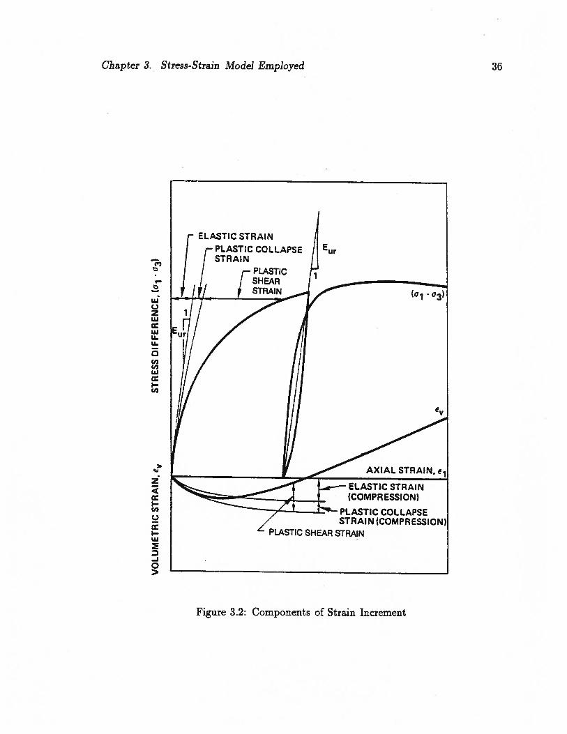
3.2 Description of the Model
Generally the total strain increment, de of a soil element can be expressed as a summa
tion of an elastic component, dee and a plastic component, den. In the stress-strain
model developed in this study, the plastic component is further divided into two
parts; a plastic shear component, de8 (the strain increments caused by the increase in
stress ratio) and a plastic volumetric or collapse component, dcc (the strain increment
caused by the increase in mean principal stress). Figure 3.2 schematically illustrates
these elastic, plastic shear and plastic collapse components of the total strain in a
typical triaxial compression test.
Mathematically, the total strain de can be expressed as,
de = dc9 + dcc H- dee (3.1)
These different strain components can be calculated separately; the plastic shear
strains by plastic stress-strain theory involving a conical type yield surface, the plastic
collapse strains by plastic stress-strain theory involving a cap type yield surface and
the elastic strains by Hooke’s law.
From the stress-strain theories, the strain components can be written as
{de8} = [C8] {do}
{de} [Ce] {th}
{dc6} = [Ce] {d} (3.2)
where [C8], [Cc] and [Ce] are the constitutive matrices corresponding to plastic shear,
plastic collapse and elastic strains. Combining equations 3.1 and 3.2 a stress-strain
relation for the total strain can be obtained as follows:
{de} = [[C8] H- [CC] + [CC]] {do}
Chapter 3. Stress-Strain Model Employed 36
I
cizwwUU
C,,C,,U
z
IC?,
ci
I-U
-J0>
Figure 3.2: Components of Strain Increment

Chapter 3. Stress-Strain Model Employed 37
= [C] {do} (3.3)
The theories involved in developing the [C8], [Cc] and [Ce] matrices in general
Cartesian coordinate system are explained in the next sections and at the end, the
full elasto-plastic constitutive matrix [C] is formed according to different loading
conditions.
In developing a finite element formulation, the stress-strain relation is generally
expressed as
do = [D] dE (3.4)
The above equation is an inverse of equation 3.3. Once the [C] matrix is known, the
[D] matrix can be easily obtained as the inverse of [C].
3.3 Plastic Shear Strain by Cone-Type Yielding
3.3.1 Background of the Model
The stress-strain relationship for the plastic shear strain is developed based on the
cSpatial Mobilized Plane’ concept by Nakai and Matsuoka (1983). Before going into
the three dimensional conditions, a brief description of the concept of mobilized plane
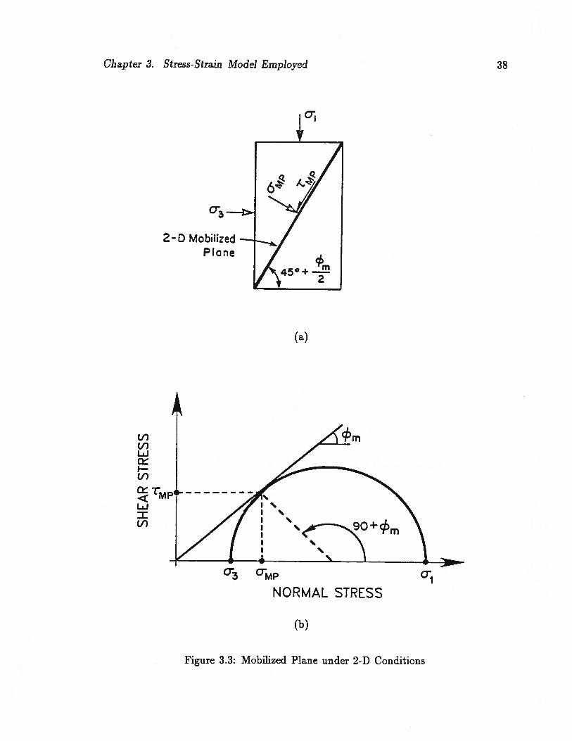
in two dimensional conditions is given to provide a better insight.
The concept of mobilized plane was first developed by Murayama (1964). The
term ‘Mobilized Plane (MP)’ refers to the plane where the shear-normal stress ratio
(rMp/crMp) is the maximum. This is the plane on which slip can be considered to
occur. The 2-D representation of this plane is shown in figure 3.3 (a). This plane
makes an angle of (45° + m/2) to the major principal stress plane, where q is the
mobilized friction angle. The Mohr circle for the stress conditions and the mobilized
friction angle are shown in figure 3.3 (b).
Chapter 3. Stress-Strain Model Employed
C,,(I,bJcC’,
TMbJ
C,,
Q3
2-D MobilizedPlane
(a)
(b)
38
Q
NORMAL STRESS
Figure 3.3: Mobilized Plane under 2-D Conditions

Chapter 3. Stress-Strain Model Employed 39
From a large number of tests and from the analysis of the shear mechanism of
granular material in a microscopic point of view, Murayama and Matsuoka (1973)
proposed a relationship between the shear-normal stress ratio (TMp /crMP) and the
normal-shear strain increment ratio (dMp/d7Mp) on the mobilized plane as,
rp (_d6MP+ (3.5)MP \ d-yf )
where ) and i are constant soil parameters. Equation 3.5 forms the basis for the
developments of the constitutive models later by Matsuoka and his co-workers.
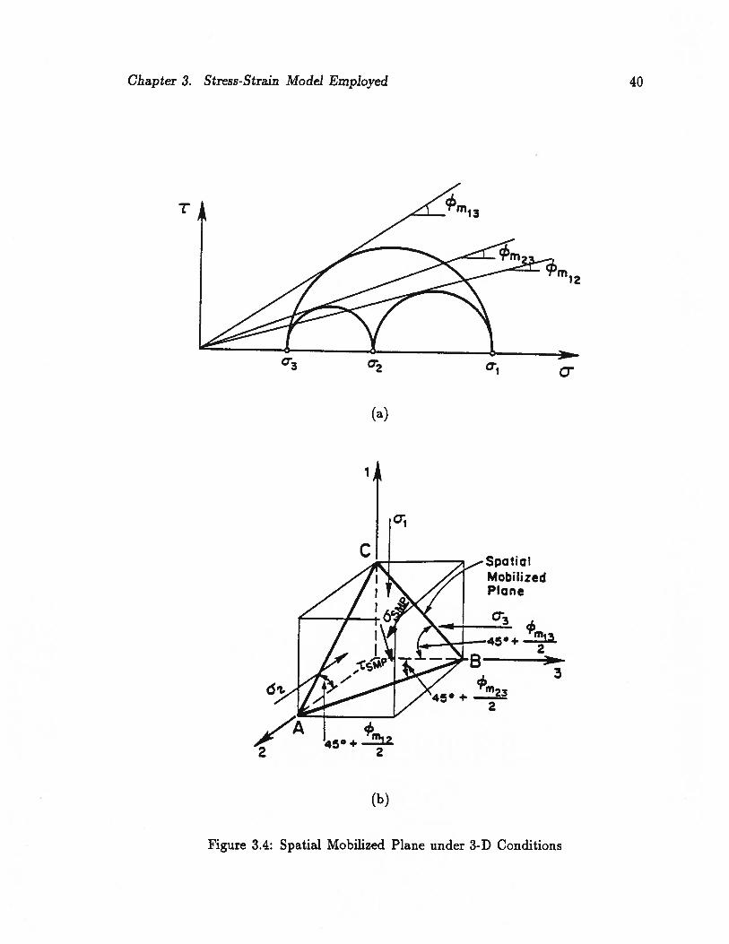
Under general three dimensional conditions, the stress state of a soil element can
be characterized by the three principal stresses o, 02 and o. Mohr circles for these
three stresses can be drawn as shown in figure 3.4 (a) and three mobilized friction
angles, ml2,4m23 and ç3 can be obtained. These mobilized friction angles can be
expressed by the following equation:
tan(450+) Z (i,j=1,2,3;ucT) (3.6)
Using these mobilized friction angles, a 3-D plane ABC can be constructed as
shown in figure 3.4 (b). This plane ABC is considered to be the plane where the
soil particles are most mobilized and is called the ‘Spatial Mobilized Plane (SMP)’.
Under isotropic stress condition (o = = 03) the mobilized plane will coincide with
the octahedral plane and will vary with possible changes in stresses. The direction
cosines of the SMP are given by the following equation:
a=
(i = 1,2,3) (3.7)
where 11,12 and 13 are the first, second and third effective stress invariants and ex
pressed by the following equations in terms of principal stresses or the stresses in the
general coordinate system.
Chapter 3. Stress-Strain Model Employed 40
r 13
m12
o•1
(a)
1
Ia;cI-f-———---———--y.— Spatial
Mobilized
V’ Plane
6 O3
—
- B7
m23450+
2
A7’ L5•+2(b)
Figure 3.4: Spatial Mobilized Plane under 3-D Conditions
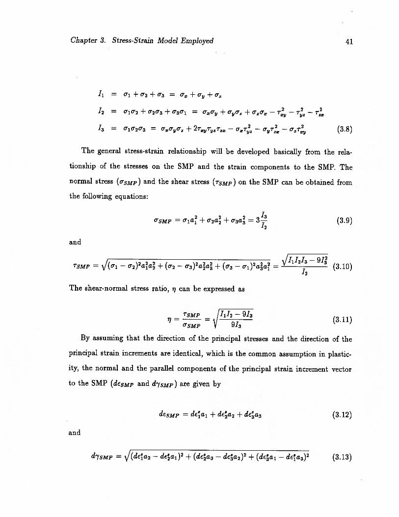
Chapter 3. Stress-Strain Model Employed 41
‘1 = O1+02+03 =
12 = 12 + 0203 + O301 = 0x0y + 0y0z + 0z0 — — T2—
13 = °y°z +2TTyzTz — OT —— OzTy (3.8)
The general stress-strain relationship will be developed basically from the rela
tionship of the stresses on the SMP and the strain components to the SMP. The
normal stress (oSMP) and the shear stress (TSMp) on the SMP can be obtained from
the following equations:
SMP = o1a + o2a + o3a = 3 (3.9)
and
\/111213 — 9ITSMp = /(oi —o2)2a?a + (o2 —o3)2aa + (o — O1)21
= ‘2(3.10)
The shear-normal stress ratio, i can be expressed as
= TSMp = I1I2 —913(3.11)
SMP 913
By assuming that the direction of the principal stresses and the direction of the
principal strain increments are identical, which is the common assumption in plastic
ity, the normal and the parallel components of the principal strain increment vector
to the SMP (dcsMp and d7sMp) are given by
dEsMp = dea1 + dea2 + dEa3 (3.12)
and
d7sMp = i,J(dEa2 — d€a1)2+ (deas — dca2)2-- (d€ai — d€1a3)2 (3.13)
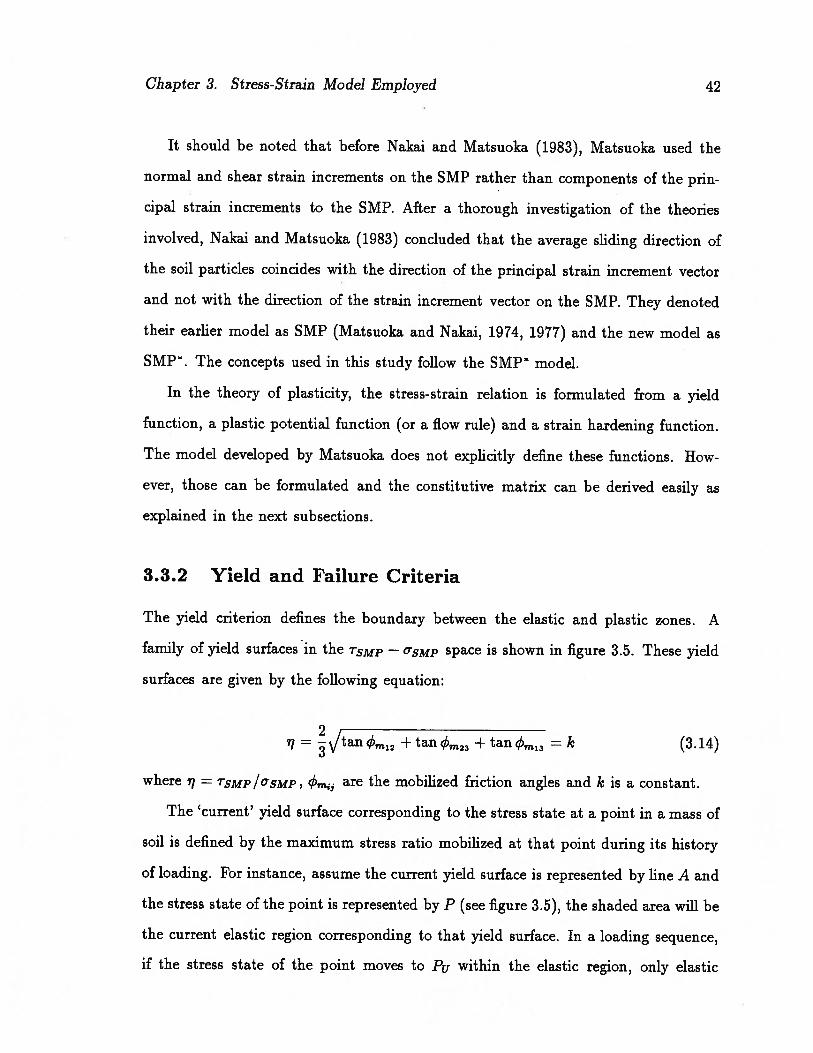
Chapter 3. Stress-Strain Model Employed 42
It should be noted that before Nakai and Matsuoka (1983), Matsuoka used the
normal and shear strain increments on the SMP rather than components of the prin
cipal strain increments to the SMP. After a thorough investigation of the theories
involved, Nakai and Matsuoka (1983) concluded that the average sliding direction of
the soil particles coincides with the direction of the principal strain increment vector
and not with the direction of the strain increment vector on the SMP. They denoted
their earlier model as SMP (Matsuoka and Nakai, 1974, 1977) and the new model as
SMP’. The concepts used in this study follow the SMP model.
In the theory of plasticity, the stress-strain relation is formulated from a yield
function, a plastic potential function (or a flow rule) and a strain hardening function.
The model developed by Matsuoka does not explicitly define these functions. How
ever, those can be formulated and the constitutive matrix can be derived easily as
explained in the next subsections.
3.3.2 Yield and Failure Criteria
The yield criterion defines the boundary between the elastic and plastic zones. A
family of yield surfaces in the TSMp — 0SMP space is shown in figure 3.5. These yield
surfaces are given by the following equation:
77—3\/tanmi2+ tan m23 + tanqm13 = k (3.14)
where i TsMp /0sMP, q5m are the mobilized friction angles and k is a constant.
The ‘current’ yield surface corresponding to the stress state at a point in a mass of
soil is defined by the maximum stress ratio mobilized at that point during its history
of loading. For instance, assume the current yield surface is represented by line A and
the stress state of the point is represented by P (see figure 3.5), the shaded area will be
the current elastic region corresponding to that yield surface. In a loading sequence,
if the stress state of the point moves to Pu within the elastic region, only elastic

Chapter 3. Stress-Strain Model Employed 43
Failure Surface
B
Yield Surfaces
A
P...
ElastIc Region
°SMP
Figure 3.5: Yield and Failure Criteria on TsMp — 05MP Space
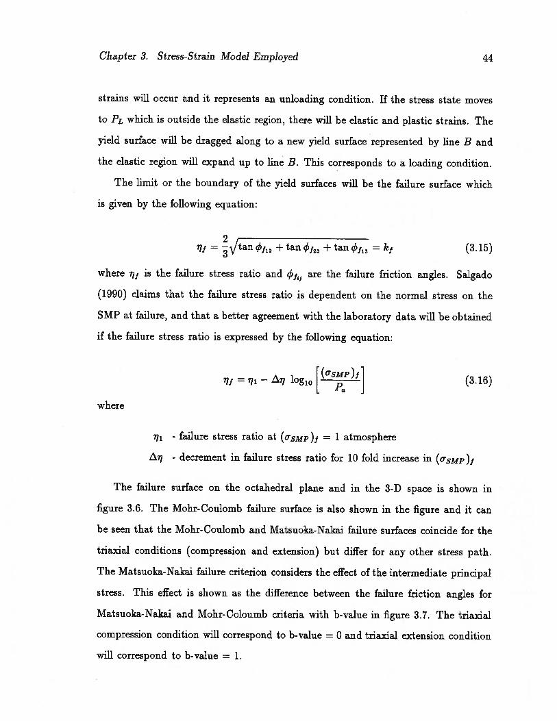
Chapter 3. Stress-Strain Model Employed 44
strains will occur and it represents an unloading condition. If the stress state moves
to FL which is outside the elastic region, there will be elastic and plastic strains. The
yield surface will be dragged along to a new yield surface represented by line B and
the elastic region will expand up to line B. This corresponds to a loading condition.
The limit or the boundary of the yield surfaces will be the failure surface which
is given by the following equation:
tan f12 + tan f23 + tan f13 = kf (3.15)
where is the failure stress ratio and are the failure friction angles. Salgado
(1990) claims that the failure stress ratio is dependent on the normal stress on the
SMP at failure, and that a better agreement with the laboratory data will be obtained
if the failure stress ratio is expressed by the following equation:
(asMP)f= — log10 (3.16)
where
- failure stress ratio at (osMp ) = 1 atmosphere
- decrement in failure stress ratio for 10 fold increase in (oSMp )
The failure surface on the octahedral plane and in the 3-D space is shown in
figure 3.6. The Mohr-Coulomb failure surface is also shown in the figure and it can
be seen that the Mohr-Coulomb and Matsuoka-Nakai failure surfaces coincide for the
triaxial conditions (compression and extension) but differ for any other stress path.
The Matsuoka-Nakai failure criterion considers the effect of the intermediate principal
stress. This effect is shown as the difference between the failure friction angles for
Matsuoka-Nakai and Mohr-Coloumb criteria with b-value in figure 3.7. The triaxial
compression condition will correspond to b-value = 0 and triaxial extension condition
will correspond to b-value = 1.
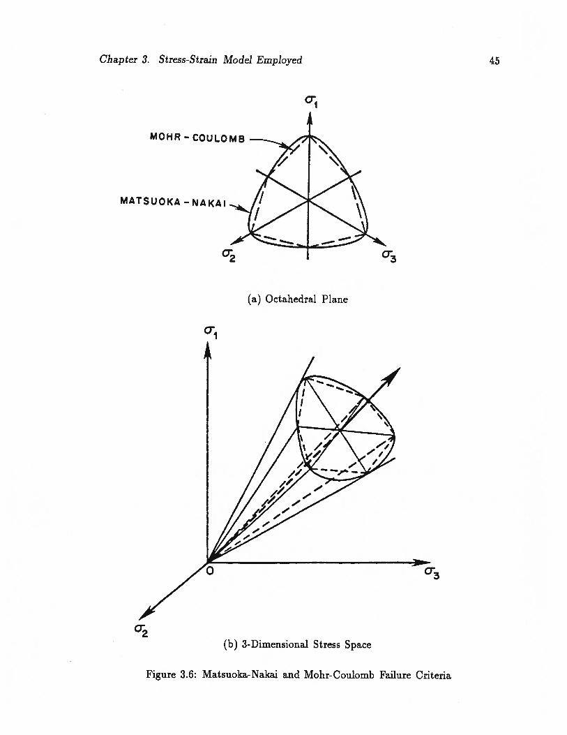
Chapter 3. Stress-Strain Model Employed 45
01
MOHR-COULOMB\
MATSUOKA- NAKAJ
(a) Octahedral Plane
01
/1II\ #\/L\’ “\/ A
1/ \%(II ,C/
p7C
0
(b) 3-Dimensional Stress Space
Figure 3.6: Matsuoka-Nakai and Mohr-Coulomb Failure Criteria
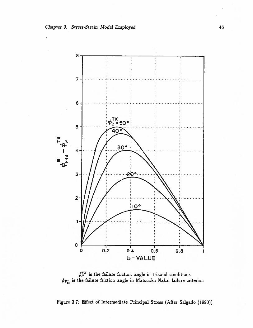
Chapter 3. Stress-Strain Model Employed 46
8-
7-
6-
TX
5..7400
-a- 3Q0:
4- .
-a-20° E
2
I0o
1- .
00 0.2 0.4 0.6 0.8
b-VALUE
çb is the failure friction angle in triaxial conditionsis the failure friction angle in Matsuoka-Nakai failure criterion
Figure 3.7: Effect of Intermediate Principal Stress (After Salgado (1990))
Chapter 3. Stress-Strain Model Employed 47
Figure 3.8: (TSMp/oSMp) Vs —(dEsMp/d7sMp) for Toyoura Sand (after Matsuoka,1983)
At a particular stress state, the ratio of the normal strain to the shear strain to
the SMP (dEsMp /d7SMp) is given by the following equation:
3.3.3 Flow Rule
The flow rule defines the direction of the plastic strain increments at every stress
state. Matsuoka’s model does not explicitly give a plastic potential function defining
the direction of plastic strain increment. Instead, a relationship for the amount of
plastic strain increment components is given, and in fact, this relationship will give
the direction of the plastic strain increment vector. An example of this relationship
obtained from triaxial compression and extension tests for Toyoura sand is shown in
figure 3.8 which is essentially a straight line. This straight line relationship holds for
all densities.
1.0
02
be”a-2
08
0.6
0.4
0.2
-0.4 -0.2 0 0.2 0.4
- ESMp “YSMP
0.6

Chapter 3. Stress-Strain Model Employed 48
[—dESMP’\?7= i , 1+11 (3.17)
\a7sMpJ
where A and t are soil parameters and is the stress ratio on the SMP.
Rewriting the above equation yields,
d6sMp(3.18)
d7sMp A
Equation 3.18 implies that the plastic strain increment vector will not be perpen
dicular to the yield surface and therefore the flow rule is nonassociative. For <
(desMp /d7sMp) will be positive which means there will be an increase in volumetric
strain for an increase in shear strain which implies contractive behaviour. For i > u,
(dEsMp/d7sMp) will be negative which indicates dilative behaviour. Figure 3.9(a)
shows the flow rule and the regions of dilative and contractive behaviour and figure
3.9(b) shows the corresponding results as desMp versus d7sMp.
3.3.4 Hardening Rule
The hardening rule defines how the threshold of yielding changes with plastic strain, or
in other words how the yield stress state changes with plastic strain. In Matsuoka’s
model, the plastic shear strain to the SMP (7sMp) is considered as the hardener.
Therefore, a relationship between i which defines the stress state and the plastic
shear strain to the SMP, 7sMP, will form the hardening rule. Matsuoka defines the
hardening rule by an empirical equation as follows:
7SMP = 7o exp (, —
(3.19)\P’ /.‘J
where i and i’ are constant soil parameters. The parameter Yo is assumed to be a
function of mean principal stress (crm) and expressed as follows:
7o -yo + Cd log10 (--) (3.20)°mi
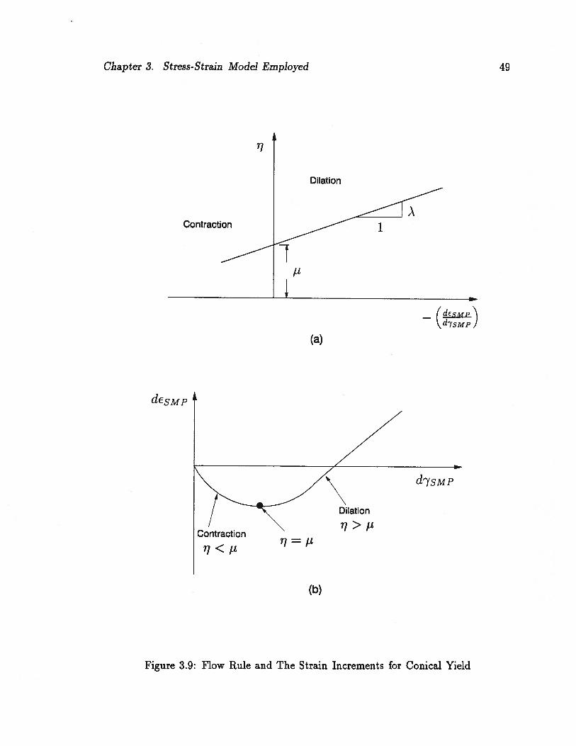
Chapter 3. Stress-Strain Model Employed 49
(a)
dEsMp
d7SM P
Dilation
71>11Contraction
“<It
(b)
Ti
Dilation
ContractionA
1
(dSMp\dy5i,jp
Figure 3.9: Flow Rule and The Strain Increments for Conical Yield

Chapter 3. Stress-Strain Model Employed 50
where Cd is a constant, omj is the initial mean principal stress and yoi is the value of
7o at 0m = 0mi An example of the hardening rule is shown in figure 3.10, which is
obtained from triaxial compression and extension tests on Toyoura sand (Matsuoka,
1983).
1.0392 kN/m2
o comp.• ext. •
2.0 3.0 4.0
Figure 3.10: rsMp/OsMp Vs YsMP for Toyoura Sand (after Matsuoka, 1983)
However, the equation 3.19 given by Matsuoka is not used in this study. Instead,
the relationship proposed by Salgado (1990) is used because, the parameters in his
relationship are more meaningful and it is easier to implement in an incremental finite
element procedure. Salgado (1990) defines the hardening rule using the hyperbolic
nature of the relationship and following the procedure by Konder (1963) as
7SMP(3.21)
+7SMP
G,. 1luUwhere

Chapter 3. Stress-Strain Model Employed 51
G,, - initial slope of the i— 7sMP curve
- stress ratio (TSMp/JSMp)
‘Tlult - asymptotic value of the stress ratio
By differentiating equation 3.21, the plastic shear strain increment /7sMP can be
obtained as,
dy5Mp = d (3.22)
where is the dimensionless tangent plastic shear parameter. This parameter is
dependent on both normal stress on SMP (crsMP) and the stress ratio. can be
evaluated by a similar procedure as given by Duncan et al. (1980) as follows:
= G(1 — Rf __)2 (3.23)1i
and
= KG(osMP)
(3.24)
where
- plastic shear number
np - plastic shear exponent
Pa - atmospheric pressure
- stress ratio
R1 - failure ratio (7f/ij,zt)
3.3.5 Development of Constitutive Matrix [CS]
The development of plastic shear constitutive matrix in terms of general Cartesian
stress and strain components from the yield criterion, hardening rule and the flow
rule is described in this section. The hardening rule (equation 3.22) and the flow rule
(equation 3.18) give the following:
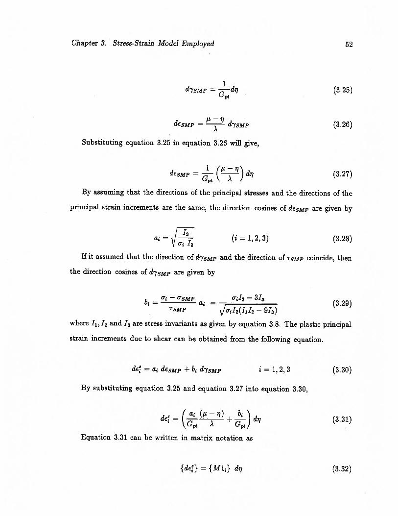
Chapter 3. Stress-Strain Model Employed 52
dysMp = —di1 (3.25)
IL—?’desMp d-y.9 (3.26)
Substituting equation 3.25 in equation 3.26 will give,
dEsMp =—
(IL ?‘) d (3.27)
By assuming that the directions of the principal stresses and the directions of the
principal strain increments are the same, the direction cosines of desMp are given by
a=
(i = 1,2,3) (3.28)
If it assumed that the direction of d7sMp and the direction of TsMp coincide, then
the direction cosines of d7sMp are given by
— SMP 0jI2 — 3131,: = = (3.29)
TSMp /o- ‘2 (I 12 — 913)
where 11,12 and 13 are stress invariants as given by equation 3.8. The plastic principal
strain increments due to shear can be obtained from the following equation.
de = a desMp H- b d7SMP i = 1,2,3 (3.30)
By substituting equation 3.25 and equation 3.27 into equation 3.30,
dE=+.i)d?’ (3.31)
Equation 3.31 can be written in matrix notation as
{defl = {M12} d?’ (3.32)

Chapter 3. Stress-Strain Model Employed 53
where M1=
+
The general Cartesian strain increments can be obtained by multiplying the prin
cipal strain increment vector by the transformation matrix, as given by the following
matrix equation:
dE l m n
de8 12 m2V
d€8d8 12 m2 n2z z z z
(3.33)d7 2l7,l, 2mm 2nn
dc2l,l 2mm2 2nn2
2l1 2m2m3
where
l, l,, and l - direction cosines of o to the x, y and z axes
m, m and m - direction cosines of 02 to the x, y and z axes
, and n - direction cosines of 03 to the x, y and z axes
Equation 3.33 can be written in matrix form as
{de8} = [MT] {dc} (3.34)
Substitution of equation 3.32 into equation 3.34 yields
{de8} = [MT] {M1} di1 (3.35)
From equation 3.11 the stress ratio on the SMP, is given by
/1112 — 913=
91(3.36)

Chapter 3. Stress-Strain Model Employed 54
By considering the invariants in terms of Cartesian stresses (equation 3.8) and
differentiating equation 3.36 with respect to Cartesian stresses the following equation
can be obtained for di7:
,
I 77 Id=
{do}
T
‘213 + 1113 (o, + o) — 1112 (o,o — r) do
1213 + 1113 (o + o) — ‘112 (o °•r — T) doy
— 1 1213 + I113(0 + o)—IiI2(t717y — r2) do-i
— 18iiI dr
—2IlI3r — 2IlI2(rr — dr
—2IlI3T — 2IiI2(rr2— or)
= {M2}T{do} (3.37)
where superscript T denote the transpose of the matrix.
Substituting equation 3.37 in equation 3.34 gives
{d68} = [MT] {M1} {M2}T {do} (3.38)
This can be further written as
{d68} = [C8] {dcr} (3.39)
where [C8] is the plastic shear constitutive matrix and will be given by
[C8] = [MT] {M1} {M2}T (3.40)
Chapter 3. Stress-Strain Model Employed 55
3.4 Plastic Collapse Strain by Cap-Type Yielding
3.4.1 Background of the Model
The plastic stress-strain theory with the conical yield surfaces described in the pre
vious section is not capable of predicting the behaviour of soil under proportional
loading. In that model, the yield surfaces are constant stress ratio lines and therefore,
for a stress path having constant stress ratio, only elastic strains will be predicted.
However, the laboratory experiments show that proportional loading with increasing
stresses causes some plastic deformation.
An additional yield surface which forms a cap on the earlier conical yield surface is
considered to circumvent this deficiency as explained in this section. The stress-strain
relationship for predicting the plastic collapse strains was developed by following the
concepts of the cap-type yielding given by Lade (1977).
As explained in section 3.2, it is reasonable to assume that the plastic collapse
strains are produced by the increase in mean normal stress and the plastic shear
strains will be associated with the shear stresses. However, under general loading con
ditions, it is difficult to separate the plastic shear and plastic collapse strains because
both will occur simultaneously. Therefore, the development of the cap-type yield
model is based on the isotropic compression tests where no plastic shear strains are
produced. Figure 3.11 shows the typical results for loading, unloading and reloading
conditions in an isotropic compression test. The elastic strains which are recoverable
can be calculated using Hooke’s law are also shown in figure 3.11. Then, the collapse
strains can be obtained by subtracting the elastic strains from the total strains.
In order to model the plastic collapse behaviour, a yield criterion which forms a
cap at the open end of the conical yield surface is used. The yield criterion and the
hardening functions for the cap-type yield are explained in the following subsections.
The stress-strain relation for the plastic collapse strain is formulated following the

Chapter 3. Stress-Strain Model Employed
E
C
‘1,w
IC,,
0
0C’)
56
Figure 3.11: Isotropic Compression Test on Loose Sacramento River Sand (after Lade,1977)
VOLUMETRIC STRAIN, eq,, (‘‘
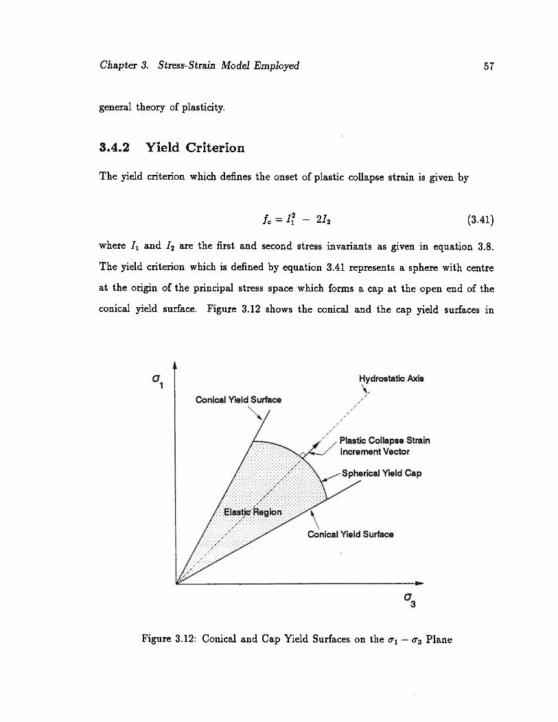
Chapter 3. Stress-Strain Model Employed 57
general theory of plasticity.
3.4.2 Yield Criterion
The yield criterion which defines the onset of plastic collapse strain is given by
f =— 212 (3.41)
where I and 12 are the first and second stress invariants as given in equation 3.8.
The yield criterion which is defined by equation 3.41 represents a sphere with centre
at the origin of the principal stress space which forms a cap at the open end of the
conical yield surface. Figure 3.12 shows the conical and the cap yield surfaces in
01 Hydrostatic Axis
Conical Yield Surface
Plastic Collapse StrainIncrement /ector
Spherical Yield Cap
Iasti Regior
Conical Yield Surface
03
Figure 3.12: Conical and Cap Yield Surfaces on the o—
03 Plane
Chapter 3. Stress-Strain Model Employed 58
the o-1 — 03 plane. The elastic region at any particular stress state will be bounded
by these two yield surfaces. As f increases beyond its current value, the yield cap
expands, soil work hardens and collapse strains are produced. It should be noted that
there are no bounds on the cap yield surface and yielding according to equation 3.41
does not result in eventual failure. The failure is entirely controlled by the conical
yield surface.
3.4.3 Flow Rule
Under isotropic compression, an isotropic soil shows equal strains in all three principal
directions. Therefore, the direction of strain increment vector should coincide with
the hydrostatic axis pointing outwards from the origin (see figure 3.12). To satisfy
this conditioi-i the plastic potential function must be identical to the yield function.
This implies the flow rule is associative and will be given by the following equation:
de = (3.42)8o.ij
where is the proportionality constant which gives the magnitude of the plastic
collapse strain and can be determined from the hardening rule.
3.4.4 Hardening Rule
The hardening rule gives a relationship between the yield function and the plastic
strain, defining how the yield function changes with plastic strain. For the cap yield
model, Lade (1977) developed an empirical relationship between the plastic collapse
work (We) and the yield function. The plastic collapse work is a function of plastic
collapse strains and given by
= J {}T{dE} (3.43)

Chapter 3. Stress-Strain Model Employed 59
The relationship between the plastic collapse work and the yield function is given
by
= CPa()P
(3.44)
where C and p are dimensionless constants and called the collapse modulus and the
collapse exponent respectively.
The proportionality constant LSX which gives the magnitude of the plastic collapse
strain increment can be obtained as follows. The increment in plastic collapse work
can be expressed as
dW = {}T {dec} (3.45)
Substitution of equation 3.42 into equation 3.45 gives
= (3.46)
Since the yield function f is a homogeneous function of degree 2, it can be shown
that
= 2f (3.47)
From equations 3.46 and 3.47, can be given as
= dWC(3.48)
3.4.5 Development of Constitutive Matrix [CC]
The constitutive matrix relating the plastic collapse strains and the stress increments
can be developed as described below. Substitution of equation 3.48 in equation 3.42
gives

Chapter 3. Stress-Strain Model Employed 60
c dW af(. )
Jc O3
By differentiating equation 3.43, dW can be obtained as
= C p a
()121
d (3.50)
and it can be further written as
dW = A df (3.51)
where A = (f)P_1
df will be obtained by differentiating 3.41 as,
df =
T
2o do
2o do
2o do= (3.52)
4r dr
4r dr
4Tz dr
By combining equations 3.49, 3.51 and 3.52 the following equation can be obtained:
A 8f 8fde = —dokj (3.53)2f 8kl
In terms of Cartesian components of stress and strain the above equation can be
written as
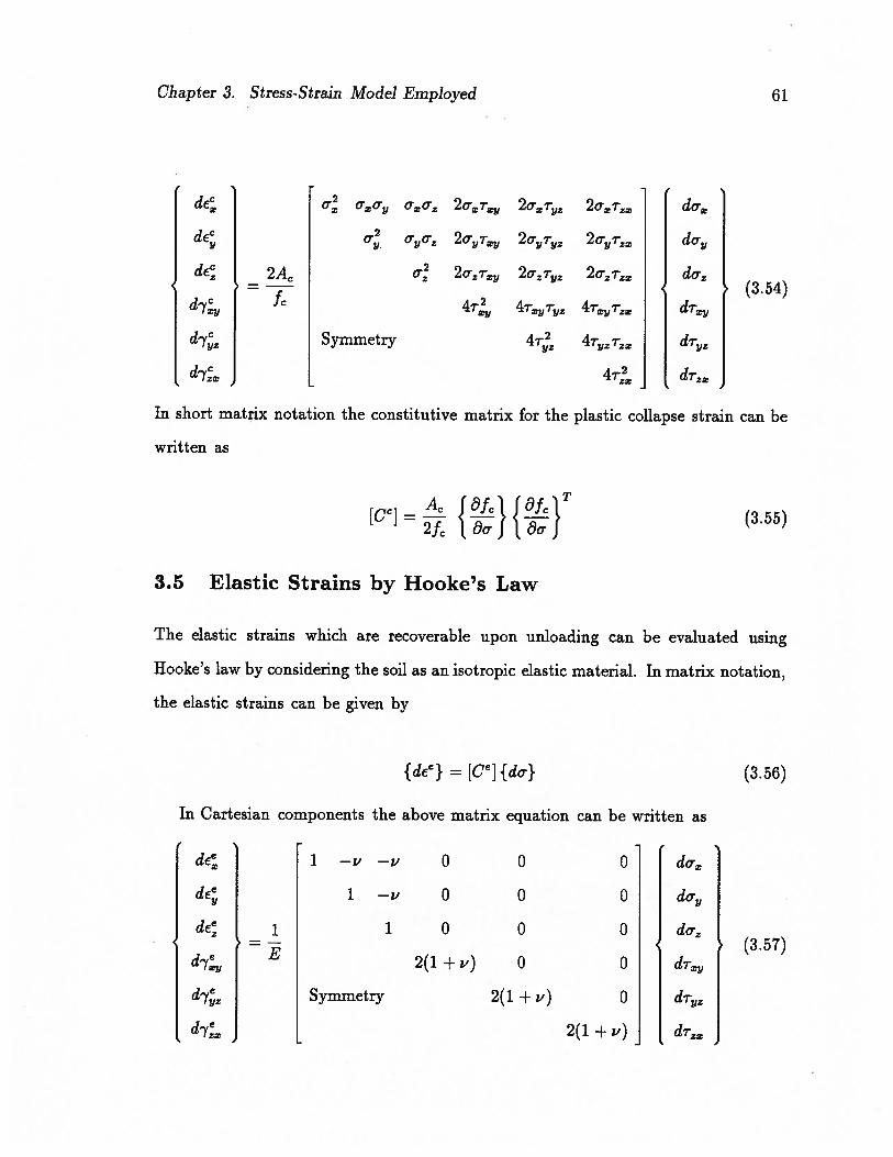
Chapter 3. Stress-Strain Model Employed 61
oo- 2or 2OTzm do
d 2or 2or22, do
dE = o 2o-2r 2o-r 2u2r do-i
d79 f 4r dT
d-y Symmetry 4r2 4r2r dr
d7 4r2 dr3,
In short matrix notation the constitutive matrix for the plastic collapse strain can be
written as
{Cc]= {8fc}{afc}T
3.5 Elastic Strains by Hooke’s Law
The elastic strains which are recoverable upon unloading can be evaluated using
Hooke’s law by considering the soil as an isotropic elastic material. In matrix notation,
the elastic strains can be given by
{dee} = [Ce] {do} (3.56)
In Cartesian components the above matrix equation can be written as
de 1 —v —v 0 0 0 do
de 1—v 0 0 0 do,
d 1 1 0 0 0 do2
(3.57)d- 2(1H-v) 0 0 dr
d72 Symmetry 2(1 + v) 0 dr2
d 2(1 + v) dr2
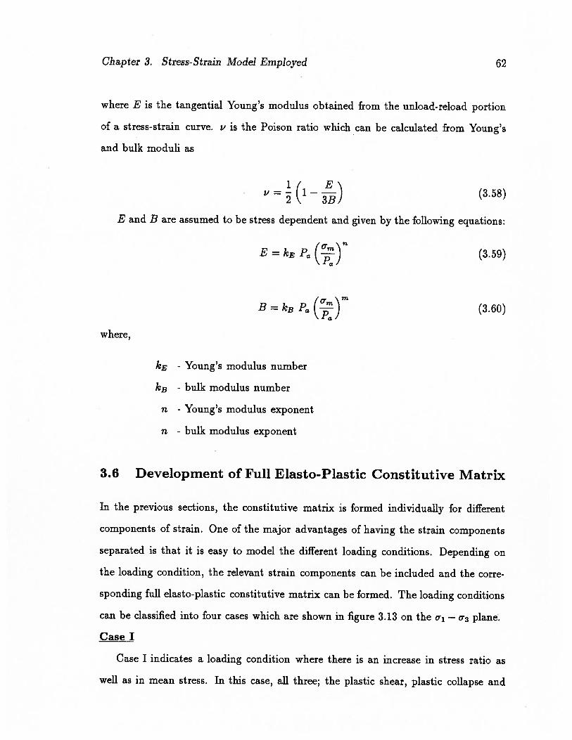
Chapter 3. Stress-Strain Model Employed 62
where E is the tangential Young’s modulus obtained from the unload-reload portion
of a stress-strain curve. i-’ is the Poison ratio which can be calculated from Young’s
and bulk moduli as
v= (i_&) (3.58)
E and B are assumed to be stress dependent and given by the following equations:
E = kE Pa()fl
(3.59)
B = Pa () (3.60)
where,
kE - Young’s modulus number
- bulk modulus number
n - Young’s modulus exponent
n - bulk modulus exponent
3.6 Development of Full Elasto-Plastic Constitutive Matrix
In the previous sections, the constitutive matrix is formed individually for different
components of strain. One of the major advantages of having the strain components
separated is that it is easy to model the different loading conditions. Depending on
the loading condition, the relevant strain components can be included and the corre
sponding full elasto-plastic constitutive matrix can be formed. The loading conditions
can be classified into four cases which are shown in figure 3.13 on the i — o plane.
Case I
Case I indicates a loading condition where there is an increase in stress ratio as
well as in mean stress. In this case, all three; the plastic shear, plastic collapse and

Chapter 3. Stress-Strain Model Employed 63
a1 Failure Surface
Ill
lastc’Rag ion
• 7
-.7.
Hydrostatic Axis
Conical Yield Surface
Failure Surface
a3
Figure 3.13: Possible Loading Conditions

Chapter 3. Stress-Strain Model Employed 64
elastic strains will be present. Then, the full elasto-plastic constitutive matrix will be
given by
[C] [[C8] + [CC] + [Ce]] (3.61)
Case II
This case considers a loading condition where there is an increase in stress ratio
and a decrease in mean stress. Here, only plastic shear and elastic strains will occur.
The full constitutive matrix will comprise those two matrices only, i.e.,
[C] = [[C8] + [CC]] (3.62)
Case III
Case III considers the loading conditions where there is a decrease in stress ratio
and an increase in mean stress. In this case, plastic collapse and elastic strains will
occur and the corresponding full constitutive matrix will be
[C] = [[CC] + [CC]] (3.63)
Case IV
Case IV indicates a complete unloading condition where there will be decrease in
both stress ratio and mean stress. Under these conditions, only elastic strains will be
recovered. Therefore, the full elasto-plastic constitutive matrix will be the same as
the constitutive matrix for the elastic strains, i.e.,
[C] = [CC] (3.64)

Chapter 3. Stress-Strain Model Employed 65
3.7 2-Dimensional Formulation of Constitutive Matrix
Generally 2-dimensional plane strain and axisymmetric analyses are more often car
ried out than 3-dimensional analyses because 3-D analysis require tedious work to
generate the relevant input data and more computer time for execution. The consti
tutive matrix for 2-D plane strain and axisymmetric conditions can be obtained easily
by imposing the appropriate boundary conditions on the 3-D constitutive matrix. A
general stress-strain relation under 3-d conditions can be given as
where C3 are
Plane Strain
Assume that the horizontal and vertical axes in the 2-D conditions are defined by
x and y. Then, all the terms associated with yz and zx and r) will
have no effect in the 2-D plane strain analysis. Hence, equation 3.65 can be reduced
to
C11 C12 C13
— C21 C22 C23
C31 C32 C33
C41 C42 C43
plane strain boundary
dc C11 C12 C13 C14
C21 C22 C23 C24
= C31 C32 C33 C34
C41 C42 C43 C44
d’y2 C51 C52 C53 C54
C61 C62 C63 C64
the components of the constitutive
C15 C16
C25 C26
C35 C36
C45 C46
C55 C56
C65 C66
matrix.
dr
do
do
dr2
drza,
(3.65)
de
dc
d6
d7
Now, by imposing the
C14 do
C24 da
C34 do
C44 dr
condition that = 0, do
(3.66)
can be
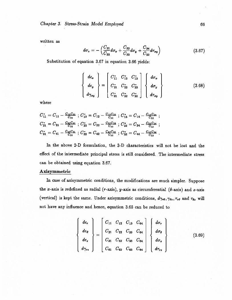
Chapter 3. Stress-Strain Model Employed 66
written as
do2 = — + do-!, + dT) (3.67)
Substitution of equation 3.67 in equation 3.66 yields:
de C1 C’2 C’3 do
de = C;1 C;2 C;3 do-u (3.68)
d C;1 C;2 C3 d
where
ri — (V C13C31 — r
_____
. C13C34‘-‘11 — ‘-‘11
—
LI12 — L112— C33 ‘ ‘—‘13 LI4
—
_______
— — C2C31 .—
(1 C,C32 .— ,- C2C3
‘—‘21 — ‘-‘21 C33 ‘ ‘-‘22 — ‘-‘22— C33 ‘ ‘-‘23 — ‘—‘24
— c,3f_I,, — f_I C43C31 . — f_I C43C32 . f_I
—f_I C43C34
— ‘-‘41— C33 ‘ ‘—‘32 — L142
— c33 ‘ ‘-‘33— C33
In the above 2-D formulation, the 3-D characteristics will not be lost and the
effect of the intermediate principal stress is still considered. The intermediate stress
can be obtained using equation 3.67.
Axisymmetric
In case of axisymmetric conditions, the modifications are much simpler. Suppose
the x-axis is redefined as radial (r-axis), y-ax.is as circumferential (0-axis) and z-axis
(vertical) is kept the same. Under axisymmetric conditions, d’yre, 7ez, r and r will
not have any influence and hence, equation 3.65 can be reduced to
dEr C11 C12 C13 C64 do.
de8 C21 C22 C23 C64 do-8(3.69)
de2 C31 C32 C33 C64 do-i
C61 C62 C63 C64 drrz
Chapter 3. Stress-Strain Model Employed 67
3.8 Inclusion of Temperature Effects
The effects of temperature changes in oil sand and the works by previous researchers
to include these effects in the analytical procedures were described in chapter 2. The
approach used by Srithar and Byrne (1991) is followed here. This involves additional
terms in the stress-strain relation and in the flow-continuity equation. The changes
which have to be made in the stress-strain relation are explained in this section.
Inclusion of temperature effects in the flow-continuity equation is described in section
5.8.
The incremental stress-strain relation can be written as
{de} = [C]{do} (3.70)
where [C] is the elasto-plastic constitutive matrix. If there is an increase in the
temperature, the sand matrix will expand and there will be additional strains. Then,
equation 3.70 will become
{d} = [C]{do} — {de8} (3.71)
where {dee}T {a d, a8 d6, a8 d6, 0, 0, 0} and a8 is the linear thermal expansion
coefficient of the sand grains and d6 is the change in temperature. It should be noted
that compressive strains are assumed positive.
By multiplying equation 3.71 by the inverse of [C] which is referred to as the
stress-strain matrix [D] the following equation can be obtained:
[D]{dc} = {dcr} — [D]{de8} (3.72)
Rearranging the terms will give
{do} = [D]{dE} + {do8} (3.73)
Chapter 3. Stress-Strain Model Employed 68
where {do-8} = [D] {de8}, which is the additional term in the stress-strain relation
due to change in temperature. This term will give the induced thermal stresses.
3.9 Modelling of Strain Softening by Load Shedding
Laboratory tests on oil sand show a decrease in strength after a peak strength is
reached which is commonly referred as strain softening. The phenomenon of strain
softening or loss of strength under progressive straining occurs because of the struc
tural changes in the material such as initiation, propagation and closure of micro
cracks. Frantziskonis and Desai (1987) stated that strain softening is not a material
property of soil when it is treated as a continuum. It is rather a performance of
the structure composed of micro-cracks and joints that result in an overall loss of
strength. When the stresses and strains deviate from homogeneity, the behaviour of
a material will no longer be represented by continuum material properties. If strain
softening is assumed as a true material property, various anomalies may arise with
respect to the solution of boundary and initial value problems. These anomalies can
lead to loss of uniqueness in the strain softening part of the stress-strain response and
to numerical instabilities as shown by Valanis (1985).
A comprehensive review of strain softening is not attempted here as it is beyond
the scope of this thesis. Reviews on this subject can be found in Read and Hegemier
(1986) and Frantziskonis (1986). In this study, the strain softening phenomenon
is modelled quantitatively using the ‘load shedding’ or ‘stress transfer’ concept. In
principle the load shedding concept is similar to the model presented by Frantziskonis
and Desai (1987). They modelled the strain softening behaviour by separating it into
two parts; a non-softening behaviour of a continuum (topical behaviour) and a damage
or stress relieved behaviour with zero stiffness. The true behaviour is estimated as
an average of these two (see figure 3.14). In finding the average behaviour, the
hydrostatic component is assumed to be the same for both parts and the deviatoric
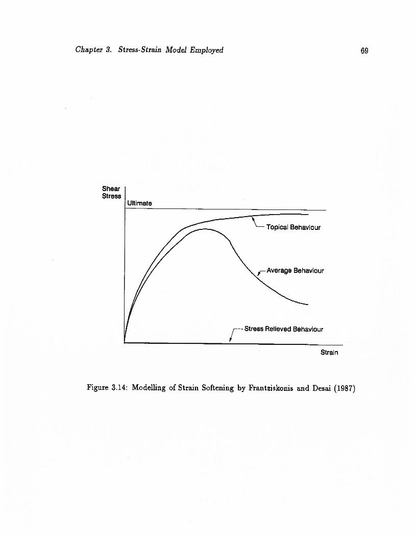
Chapter 3. Stress-Strain Model Employed 69
ShearStress
Ultimate
Topical Behaviour
— Average Behaviour
Strain
Figure 3.14: Modelling of Strain Softening by Frantziskonis and Desai (1987)

Chapter 3. Stress-Strain Model Employed 70
stress is averaged. Since the stiffness is assumed to be zero in the damage behaviour,
the deviatoric stress will be zero for that part. Thus, only the deviatoric stress from
the continuum behaviour is reduced or some of the deviatoric stress is taken away.
This is similar to the load shedding technique with constant mean stress.
In order to model the strain softening behaviour, the variation of the stress ratio
(or the strength) with the strains in the strain softening region should be established.
Here, the variation is assumed to be represented by an equation similar to that given
by Frantziskonis and Desai (1987) for their damage evolution. Thus, in the strain
softening region the stress-strain relation can be given as
= i + (ii, — ‘qr)exp{—k(ysMp—
(3.74)
where
- Residual stress ratio
- Peak stress ratio
7SMP,p - Peak shear strain
Ic, q - Constant parameters
3.9.1 Load Shedding Technique
Load shedding (Zienkiewicz et al. (1968), Byrne and Janzen (1984)) is a technique
to correct the stress state of an element which has violated the failure criterion, by
taking out the overstress and redistributing to the adjacent unfailed elements. A brief
description of how the load shedding technique is applied to model strain softening is
presented below. Details of the estimation of overstress and the corresponding load
vector are given in appendix A.
Figure 3.15 shows a typical scenario in modelling strain softening by load shedding.
The stress state of an element depicted by point P0 in the figure can move to point

Chapter 3. Stress-Strain Model Employed
‘1]
‘rip
Figure 3.15: Modelling of Strain Softening by Load Shedding
71
P1
P2
F? T
I
7r
71 7
Chapter 3. Stress-Strain Model Employed 72
P1 in a load increment. But the actual stress state should be point Pia and in order
to bring to this stress state, an overstress of should be removed. The overstress
will then be redistributed to the adjacent stiffer elements. During the redistribution
process, the modulus of the failed element will be defaulted to a low value so that it
will not take any more load. However, in another load increment the stress state may
move to point P2. Then again the stress state will be brought to point F2a by load
shedding. In the process of load shedding, it is also possible that some other elements
violate failure criteria and those loads also have to be redistributed. Therefore, several
iterations may be needed to find a solution where failure criteria are satisfied by all
the elements.
3.10 Discussion
Although the stress-strain model employed in this study is somewhat sophisticated, it
will not capture the real soil behaviour under certain loading conditions. For instance,
since the model assumes the material to be isotropic, it will not correctly predict the
deformations for pure principal stress rotations.
In the stress-strain model used in this study, the elastic principal strain increment
directions are assumed to coincide with the principal stress increment directions and
the plastic principal strain increment directions are assumed to coincide with the prin
cipal stress directions. Lade (1977) also stated that the principal strain increment
directions coincide with the principal stress increment directions at low stress levels
where elastic strains are predominant and coincide with principal stress directions at
high stress levels where plastic strains are predominant. Salgado (1990) presented a
critical review regarding the assumption that the direction of principal strain incre
ments coincide with the direction of principal stresses. He reviewed the results using
the hollow cylinder device by Symes et al. (1982, 1984, 1988) and Sayao (1989) and
concluded that the assumption is reasonably valid for most of the stress paths except

Chapter 3. Stress-Strain Model Employed 73
those that involve significant principal stress rotations.
One of the disadvantages of this model is its limited use in the past. Unlike the
hyperbolic model, information on the model parameters is very limited. The possible
range of values for some of the parameters and their physical significance are not
well defined. However, a sensitivity study on the parameters is given in chapter
4, which may be helpful to understand the physical significance of the parameters.
Another disadvantage of the model is that because of the nonassociated flow rule, it
will result in a non-symmetric stiffness matrix which requires considerable computer
memory and time. However, the frontal solution scheme used in this study will
circumvent the requirement for large memory since it does not assemble the full
stiffness matrix and requires only a small memory. Furthermore, these factors of time
and memory requirements may not be considered as disadvantages with the rapid
growth in computer capabilities.

Chapter 4
Stress-Strain Model - Parameter Evaluation and
Validation
4.1 Introduction
This chapter describes the procedures used to evaluate the soil parameters needed for
the stress-strain model and presents results verifying the stress-strain model against
measured responses in laboratory tests. The soil parameters required for the model
can be classified into four groups; elastic, plastic shear, plastic collapse and strain
softening. A summary of the parameters and their description are given in table 4.1.
The procedures used to evaluate these parameters from basic laboratory tests such
as isotropic compression and triaxial compression tests are described in section 4.2.
For the determination of some of the parameters at least two test results are necessary
to obtain a straight line fit. In those cases, it is advisable to have three or more test
results to obtain a better fit. Validations of the stress-strain model against laboratory
results on Ottawa sand and on oil sand are given in section 4.3. Sensitivity analyses
on some of the parameters have been carried out to provide some idea about their
significance and these are described in section 4.4.
4.2 Evaluation of Parameters
In this section, only the procedures for the evaluation of the parameters are given in
detail. Applications of these procedures to actual test data on Ottawa sand and on
oil sand can be found in section 4.3.
74

Chapter 4. Stress-Strain Model - Parameter Evaluation and Validation 75
Table 4.1: Summary of Soil Parameters
L Type Parameter Description
Elastic kE Young’s modulus numbern Young’s modulus exponent
kB Bulk modulus numberm Bulk modulus exponent
Plastic Shear Failure stress ratio at one atmosphereLi Decrease in failure stress ratio
for 10 fold increase in 0SMP
.\ Flow rule slope
i Flow rule interceptKG Plastic shear numbernp Plastic shear exponentR1 Failure ratio
Plastic Collapse C Collapse modulus numberp Collapse modulus exponent
Strain Softening Strain softening constantq Strain softening exponent
4.2.1 Elastic Parameters
4.2.1.1 Parameters kE and n
The elastic parameters kE and n can be determined from the unload-reload portion of
a triaxial compression test as explained by Duncan et al. (1980). To determine these
parameters, at least two unload-reload modulus values (see figure 4.1(a)) at different
mean normal stresses are necessary. The unload-reload Young’s modulus is given by
E kE Pa ()‘ (4.1)
By rearranging and taking the logarithm, the above equation can be written as
log (-) = log kE + n log (i) (4.2)
Thus, kE and n can be determined by plotting (E/Pa) against (0m/1Zba) on a log-log

Chapter 4. Stress-Strain Model - Parameter Evaluation and Validation 76
plot as shown in figure 4.1(b).
In the standard triaxial compression test, the unload-reload stress path is often not
performed. In the absence of unload-reload results, kE for the unload-reload portion
can be roughly estimated from (kE) for primary loading. The values of (k) can be
found in Duncan et al. (1980) and in Byrne et al. (1987) for various soils. Duncan et
al. claimed that the ratio of kE/(kE) varies from about 1.2 for stiff soils such as dense
sands up to about 3 for soft soils such as loose sands. The value of the exponent n for
unload-reload is found to be almost the same as the exponent for primary loading.
Hence, if the value of n is known, kE can be determined from a single unload-reload
E value.
4.2.1.2 Parameters kB and m
The best way of evaluating kE and m is from the unload-reload results of an isotropic
compression test. The procedure proposed by Byrne and Eldrige (1982) is followed
here to determine these parameters. The volumetric strain and the mean stress in
the unload-reload path can be related as
= a (°m)’ (4.3)
where a and b are constants and can be obtained by plotting versus 0m on a log-log
scale as shown in figure 4.2.
Differentiation of equation 4.3 yields
ck 1 b—i (4.4)
Then, the bulk modulus B can be expressed as
B = (Om)1 (45)

Chapter 4. Stress-Strain Model - Parameter Evaluation and Validation 77
q-a3 /AE1
€
(a) Unload-Reload Modulus
(E/Pa)
1000
100
‘<E ‘a
1 10(ojP)[log scale] . a
(b) Variation of E with a3
Figure 4.1: Evaluation of kE and n

Chapter 4. Stress-Strain Model - Parameter Evaluation and Validation 78
0.01 -
kB = a.b(Pa)6
a m=1-b
100[log scale]
Figure 4.2: Evaluation of kB and m

Chapter 4. Stress-Strain Model - Parameter Evaluation and Validation 79
The general expression for B is given by
B = kBPa()
(4.6)
By considering the similarities of equations 4.5 and 4.6, the parameters kB and m
can be obtained from a and b as
m=1—b (4.7)
kB= ab(Pa)’
(4.8)
It should be noted that the parameters kE and kB can be related by the Poisson’s
ratio v as
kB= 3(1—2zi)
(4.9)
Hence, by knowing one parameter, the other one can also be determined from
the Poisson’s ratio. Lade (1977) stated that the Poisson’s ratio for the unload-reload
path has often been found to be close to 0.2.
4.2.2 Evaluation of Plastic Collapse Parameters
Only two parameters are needed to evaluate the plastic collapse strains. These two
parameters define the hardening law and can be determined from an isotropic com
pression test. The hardening law is given by
= CPa ()‘ (4.10)
where W is the plastic collapse work, f defines the yield surface and C and p
are constant parameters to be determined. For the isotropic compression loading
condition, f and W will be given by

Chapter 4. Stress-Strain Model - Parameter Evaluation and Validation 80
f = 3o (4.11)
Wc=Jcr3de (4.12)
where de = d€,, — d and de is the elastic volumetric strain.
By plotting W/P against f/P on a log-log plot, the parameters C and p can
be obtained as shown in figure 4.3.
0.01 -
[log scale]
Figure 4.3: Evaluation of C and p
4.2.3 Evaluation of Plastic Shear Parameters
In determining the plastic shear parameters, it is easier to divide them into three
groups as follows:
1. Failure parameters i and LSi

Chapter 4. Stress-Strain Model - Parameter Evaluation and Validation 81
2. Flow rule parameters i and )
3. Hardening rule parameters KG, np and R1
The plastic shear parameters can be determined from all types of tests where the
principal stresses and principal strains can be obtained. By knowing the principal
stresses and strains, the stresses and strains on the spatial mobilized plane (SMP)
can be evaluated as described in section 3.3. The plastic shear parameters can then
be obtained as explained in the following subsections.
The most common laboratory shear tests performed are triaxial compression tests
and therefore, special attention is given here to describe how to obtain the plastic
shear parameters from those test results.
Firstly, the elastic and plastic collapse strains have to be subtracted to obtain the
principal plastic shear strains:
d = de1 — de — (4.13)
d€ = de3 — de — d (4.14)
Under standard triaxial compression conditions, the elastic and plastic collapse
strains can be given by
do1(4.15)
de = —vde (4.16)
de = o do1 (4.17)
d = 2A u1o3 do (4.18)
where2C (p 1—2p
— P\ a)
—
(o + 2o)2P

Chapter 4. Stress-Strain Model - Parameter Evaluation and Validation 82
It should be noted that if the test samples are preconsolidated to a higher stress
and unloaded, then the collapse strains should not be subtracted.
By following the equations in section 3.3.1 and imposing the conditions for triaxial
compression loading, the stresses and the strains related to SMP can be obtained as
follows:3o-1o3
SMP = (4.19)•1 + 03
TSMp(4.20)
SMP 3
— dc/ + 2d4/dEsMp — (4.21)
/2o + o
2(deW — de/jd7sMp = (4.22)
2o1+c3
4.2.3.1 Evaluation of q’ and z
At least two tests up to failure at different confining stresses are necessary to determine
these parameters. The failure stress ratio on SMP is given by
(o-sMP)f= — Li log10Pa
(4.23)
The values of and (OsMP)f can be obtained using equations 4.20 and 4.19. By
plotting {(OSMp)f/Pal versus on a semi-log plot, i and ii can be determined as
shown in figure 4.4.
4.2.3.2 Evaluation ofi and X
The flow rule for the plastic shear is expressed by the following equation.
f—c1EsMpi J+/L (4.24)\ u7SMP J
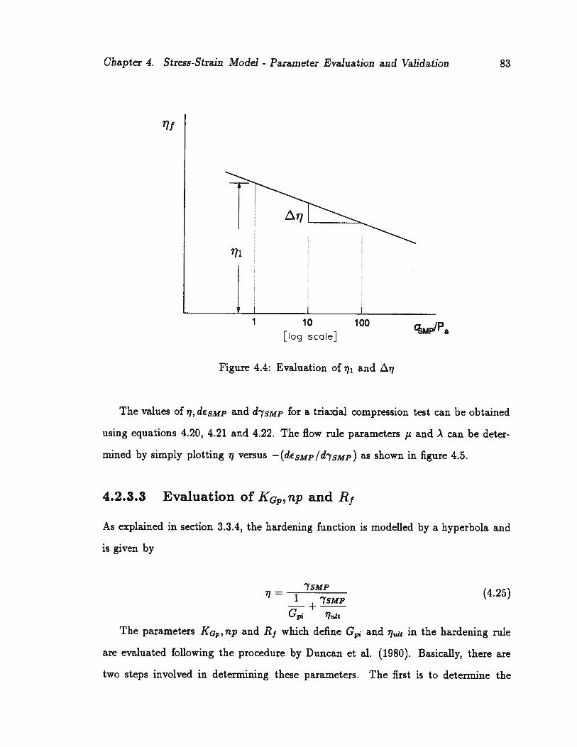
Chapter 4. Stress-Strain Model - Parameter Evaluation and Validation 83
‘if
____
—
_________ ______
1 10 100e’ a[log scale]
Figure 4.4: Evaluation of 1h and ‘i
The values of i, dEsMp and d7sMp for a triaxial compression test can be obtained
using equations 4.20, 4.21 and 4.22. The flow rule parameters and ) can be deter
mined by simply plotting versus —(desMp/d7sMp) as shown in figure 4.5.
4.2.3.3 Evaluation of KG,rIp and Rf
As explained in section 3.3.4, the hardening function is modelled by a hyperbola and
is given by
7SMP17 = (4.25)
+G.The parameters KG, np and R1 which define C and it in the hardening rule
are evaluated following the procedure by Duncan et al. (1980). Basically, there are
two steps involved in determining these parameters. The first is to determine the
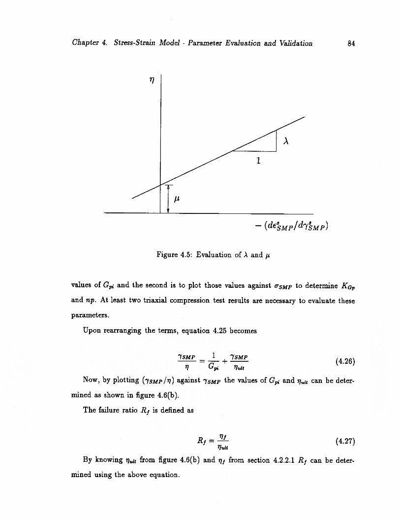
Chapter 4. Stress-Strain Model - Parameter Evaluation and Validation 84
‘17
— (dEMp/d4Mp)
Figure 4.5: Evaluation of ) and t
values of G, and the second is to plot those values against °5Mp to determine KG
and np. At least two triaxial compression test results are necessary to evaluate these
parameters.
Upon rearranging the terms, equation 4.25 becomes
7SMP — 1 7SMP4 26
1 7u1t
Now, by plotting (7sMp/7/) against fsMP the values of G7, and 71,jit can be deter
mined as shown in figure 4.6(b).
The failure ratio Rf is defined as
Rf (4.27)l7ult
By knowing from figure 4.6(b) and i from section 4.2.2.1 Rf can be deter
mined using the above equation.
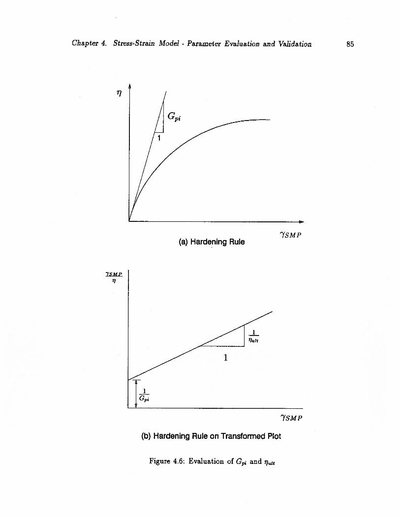
Chapter 4. Stress-Strain Model - Parameter Evaluation and Validation 85
“7
1
7SMP(a) Hardening Rule
7SMP
‘1
G1
7SMP
(b) Hardening Rule on Transformed Plot
Figure 4.6: Evaluation of G and ij
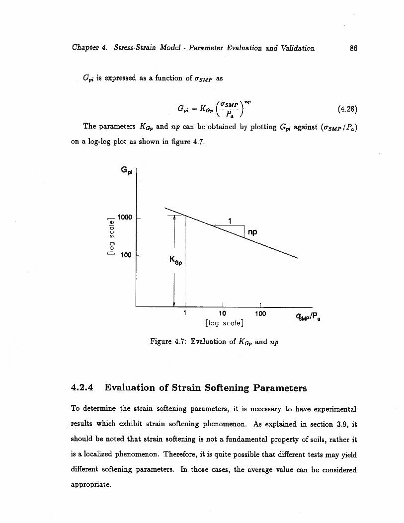
Chapter 4. Stress-Strain Model - Parameter Evaluation and Validation 86
G is expressed as a function of op as
G = KG (4.28)
The parameters KG and np can be obtained by plotting G,. against (oSMp/Pa)
on a log-log plot as shown in figure 4.7.
1000‘1)0c-I(I)
0U 100
1 10 100[log scale]
Figure 4.7: Evaluation of K0 and np
MP’a
4.2.4 Evaluation of Strain Softening Parameters
To determine the strain softening parameters, it is necessary to have experimental
results which exhibit strain softening phenomenon. As explained in section 3.9, it
should be noted that strain softening is not a fundamental property of soils, rather it
is a localized phenomenon. Therefore, it is quite possible that different tests may yield
different softening parameters. In those cases, the average value can be considered
appropriate.
1
np
KQ
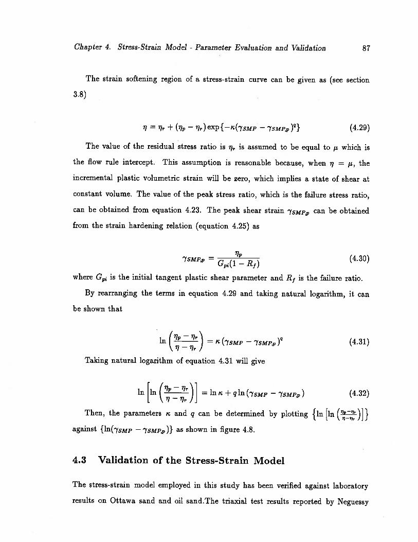
Chapter 4. Stress-Strain Model - Parameter Evaluation and Validation 87
The strain softening region of a stress-strain curve can be given as (see section
3.8)
= ir + (ip— lir) exp{—i(7sMp
— 7SMP,p)} (4.29)
The value of the residual stress ratio is i is assumed to be equal to t which is
the flow rule intercept. This assumption is reasonable because, when i = p, the
incremental plastic volumetric strain will be zero, which implies a state of shear at
constant volume. The value of the peak stress ratio, which is the failure stress ratio,
can be obtained from equation 4.23. The peak shear strain 7SMp can be obtained
from the strain hardening relation (equation 4.25) as
7737SMP,p = (4.30)
G1 — R11
where is the initial tangent plastic shear parameter and Rf is the failure ratio.
By rearranging the terms in equation 4.29 and taking natural logarithm, it can
be shown that
in () K(7sMp (4.31)
Taking natural logarithm of equation 4.31 will give
ln [in(ij]
ln + qln(7sMp— 7sMp,p) (4.32)
Then, the parameters , and q can be determined by plotting {ln [ln ()] }against {ln(7sMp — 7SMP,p )} as shown in figure 4.8.
4.3 Validation of the Stress-Strain Model
The stress-strain model employed in this study has been verified against laboratory
results on Ottawa sand and oil sand.The triaxial test results reported by Neguessy
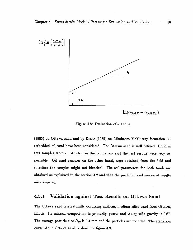
Chapter 4. Stress-Strain Model - Parameter Evaluation and Validation 88
in [in (TZr)]
Figure 4.8: Evaluation of i and q
(1985) on Ottawa sand and by Kosar (1989) on Athabasca McMurray formation in
terbedded oil sand have been considered. The Ottawa sand is well defined. Uniform
test samples were constituted in the laboratory and the test results were very re
peatable. Oil sand samples on the other hand, were obtained from the field and
therefore the samples might not identical. The soil parameters for both sands are
obtained as explained in the section 4.2 and then the predicted and measured results
are compared.
4.3.1 Validation against Test Results on Ottawa Sand
The Ottawa sand is a naturally occurring uniform, medium silica sand from Ottawa,
illinois. Its mineral composition is primarily quartz and the specific gravity is 2.67.
The average particle size D50 is 0.4 mm and the particles are rounded. The gradation
curve of the Ottawa sand is shown in figure 4.9.
q
in(7sMp— 7SMP,p)
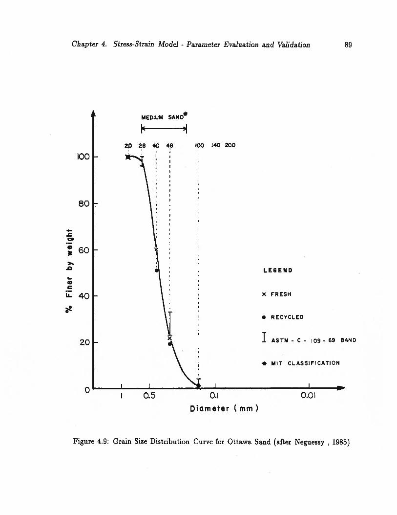
Chapter 4. Stress-Strain Model - Parameter Evaluation and Validation
zp ae 4 48 100
‘ I
I I
I I
89
MEDIUM SAND
‘I
I00
140 200
80
60
C
t4Q
LEGE ND
X FRESH
20
• RECYCLED
I
0
ASTM - C - 109- 69 BAND
* MIT CLASSIFICATION
I 0.5 0.1 0.01
Diameter (mm)
Figure 4.9: Grain Size Distribution Curve for Ottawa Sand (after Neguessy , 1985)

Chapter 4. Stress-Strain Model - Parameter Evaluation and Validation 90
The following test results reported by Negussey (1985) are considered here for the
determination of the relevant parameters and for the validation:
1. Resonant column tests
2. Isotropic compression tests
3. Triaxial compression tests
4. Proportional loading tests (R = o1/o3 = 1.67 and 2)
5. Tests along four different stress paths as shown in figure 4.10
SP4
300 SP3
a.
200
SP2SP1- = 2.0
SP2- (a/u=4.0spi100 SP3 - P
= 250 kPa, Constant
SP4 - P’ = 350 kPa, Constant
100 200 300 400
UH(kPa)
Figure 4.10: Stress Paths Investigated on Ottawa Sand
The test results considered here are for Dr = 50%. The maximum and minimum
void ratios of the Ottawa sand are 0.82 and 0.50 respectively.

Chapter 4. Stress-Strain Model - Parameter Evaluation and Validation
4.3.1.1 Parameters for Ottawa Sand
91
As explained in section 4.2.1, the Young’s modulus values for different confining
stresses are plotted in figure 4.11. The values plotted in the figure are from resonant
:-
(kE)p= 1180
- . Resonant Column -
-
A Tria)_(UnIoad Reload)
— •Triaxlal (Primary Loading)
I I I
a3 a
Figure 4.11: Variation of Young’s moduli with confining stresses
column tests which yield similar values as are obtained in unload-reload tests. Also
shown in the figure are one unload-reload modulus and the Young’ modulus values
for primary loading from standard triaxial compression tests. It can be seen that the
unload-reload value agrees well with the resonant column values. The ratio of the
Young’s modulus for the primary loading condition to the unload-reload condition is
about 2.2 and the exponent for both conditions is 0.46. This agrees with the statement
by Duncan et al. (1980) that the ratio of Young’s moduli varies from about 1.2 for
dense sands to about 3 for loose sands. From figure 4.11 the values for kE and n can
10000
5000
3000
2000
1000
5000.3 0.5 1 2 3 5 10
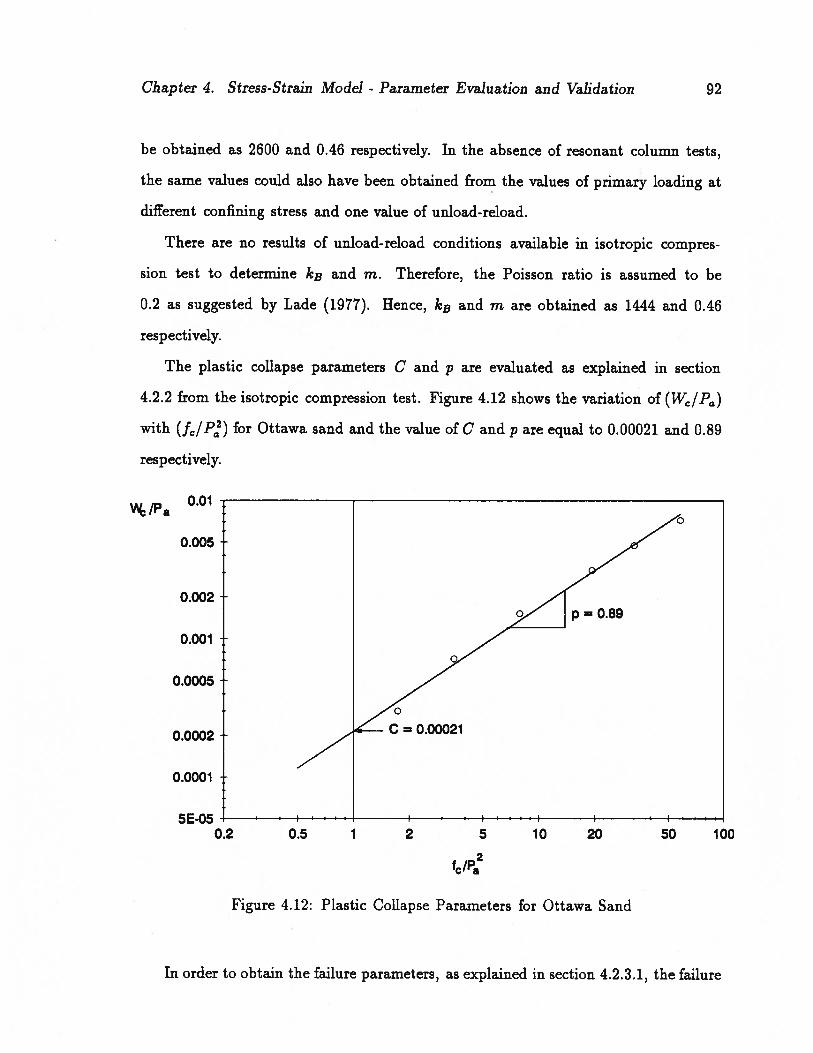
Chapter 4. Stress-Strain Model - Parameter Evaluation and Validation 92
be obtained as 2600 and 0.46 respectively. In the absence of resonant column tests,
the same values could also have been obtained from the values of primary loading at
different confining stress and one value of unload-reload.
There are no results of unload-reload conditions available in isotropic compres
sion test to determine kB and m. Therefore, the Poisson ratio is assumed to be
0.2 as suggested by Lade (1977). Hence, kB and m are obtained as 1444 and 0.46
respectively.
The plastic collapse parameters C and p are evaluated as explained in section
4.2.2 from the isotropic compression test. Figure 4.12 shows the variation of (We/Pa)
with (fe/P) for Ottawa sand and the value of C and p are equal to 0.00021 and 0.89
respectively.
0.01We/Pa
0.005
0.002
0.00 1
0.0005
0.0002
0.0001
5E-050.2 0.5 1 2 5 10 20
2
50 100
Figure 4.12: Plastic Collapse Parameters for Ottawa Sand
In order to obtain the failure parameters, as explained in section 4.2.3.1, the failure

Chapter 4. Stress-Strain Model - Parameter Evaluation and Validation 93
stress ratio i vs usMp for the triaxial compression test results are plotted in figure
4.13. The failure parameters () and ZSi7 are determined as 0.49 and 0.0.
Figure 4.13: Failure Parameters for Ottawa Sand
The four triaxial compression test results are shown as vs. (—desMp/d7sMp) in
figure 4.14 to determine the flow rule parameters A and p (refer to section 4.2.3.2).
From the figure, p and A are obtained as 0.26 and 0.85 respectively.
As explained in section 4.2.3.3, for the evaluation of hardening rule parameters,
the results from the triaxial compression tests are transformed and the relevant plots
are shown in figure 4.15. The value of R1 is determined as 0.93. From figure 4.15(c),
the values of KG and np are obtained as 780 and —0.238 respectively.
Table 4.2 summarizes all the parameters for Ottawa sand at Dr = 50%.
Ti
0.6
0.5
0.4
0.3
0.2
0.1
—— —71iO49
ö::
zS7=O.O
1000.5 1 2 3 5
cTSMP/P
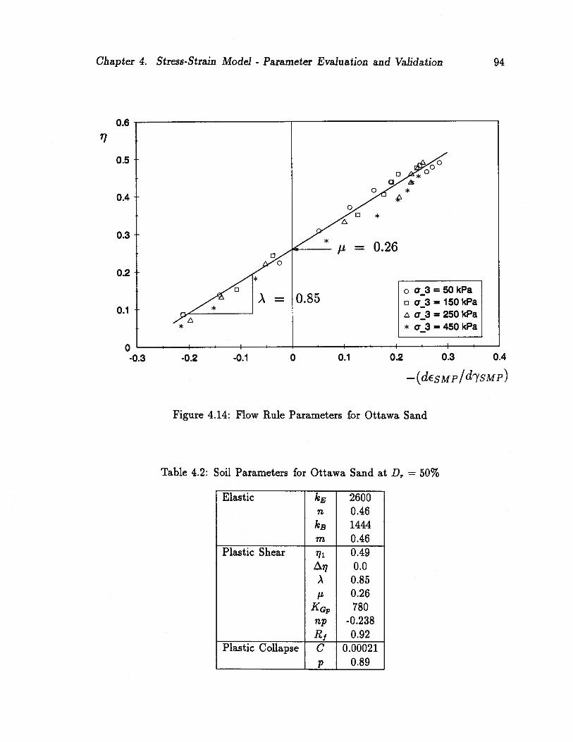
Chapter 4. Stress-Strain Model - Parameter Evaluation and Validation 94
Table 4.2: Soil Parameters for Ottawa Sand at D = 50%
Elastic kE 2600n 0.46kB 1444
m 0.46Plastic Shear 0.49
1117 0.0X 0.85u 0.26
780np -0.238
Rf 0.92Plastic Collapse C 0.00021
p 0.89
‘7
0.6
0.5
0.4
03
0.2
0.1
0-0.3 -0.2 -0.1 0 0.1 0.2 0.3
_(dEsMp/d7sMP)
0.4
Figure 4.14: Flow Rule Parameters for Ottawa Sand

Chapter 4. Stress-Strain Model - Parameter Evaluation and Validation 95
(a)0.5
0.4
___________
o3=5OkPa0.3 ,‘ ---0---
3=150kPa02 —
• a_3=50kPa
0.1 I a3=45OkPa--.“---.-
00 0.2 0.4 0.6 0.8
7SMP
1.87SMP
1.6 o
1,4
1.2
1
0.8
0.6
0.4
0.2 ‘
0 I I
0 0.2 0.4 0.6 0.87SMP
800G1
750.W 735%% ‘UP
700
650
600Jlr=0.145
550
500 I I I
0.5 1 2 3 5 10
Figure 4.15: Hardening Rule Parameters for Ottawa Sand
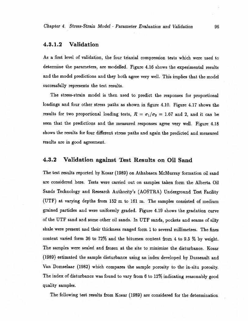
Chapter 4. Stress-Strain Model - Parameter Evaluation and Validation 96
4.3.1.2 Validation
As a first level of validation, the four triaxial compression tests which were used to
determine the parameters, are modelled. Figure 4.16 shows the experimental results
and the model predictions and they both agree very well. This implies that the model
successfully represents the test results.
The stress-strain model is then used to predict the responses for proportional
loadings and four other stress paths as shown in figure 4.10. Figure 4.17 shows the
results for two proportional loading tests, R = o1/o3 = 1.67 and 2, and it can be
seen that the predictions and the measured responses agree very well. Figure 4.18
shows the results for four different stress paths and again the predicted and measured
results are in good agreement.
4.3.2 Validation against Test Results on Oil Sand
The test results reported by Kosar (1989) on Athabasca McMurray formation oil sand
are considered here. Tests were carried out on samples taken form the Alberta Oil
Sands Technology and Research Authority’s (AOSTRA) Underground Test Facility
(UTF) at varying depths from 152 m to 161 m. The samples consisted of medium
grained particles and were uniformly graded. Figure 4.19 shows the gradation curve
of the UTF sand and some other oil sands. In UTF sands, pockets and seams of silty
shale were present and their thickness ranged form 1 to several millimetres. The fines
content varied form 36 to 72% and the bitumen content from 4 to 9.5 % by weight.
The samples were sealed and frozen at the site to minimize the disturbance. Kosar
(1989) estimated the sample disturbance using an index developed by Dusseault and
Van Domselaar (1982) which compares the sample porosity to the in-situ porosity.
The index of disturbance was found to vary from 6 to 12% indicating reasonably good
quality samples.
The following test results from Kosar (1989) are considered for the determination

Chapter 4. Stress-Strain Model - Parameter Evaluation and Validation
00
0
97
a 3 = 50 kPa----*--
a_3• = 5O kPa
o 3 = 250 kPa-------
800
600 - _..
0400- — .0
200 -
I I
a_3 =50 kPa
Symbols - ExperimentalLines - Analytical
(a)
0.05
0.>
‘U
0.15
0.2
0.250 0.2 0.4 0.6 0.8
E(%)a
Figure 4.16: Results for Triaxial Compression on Ottawa Sand
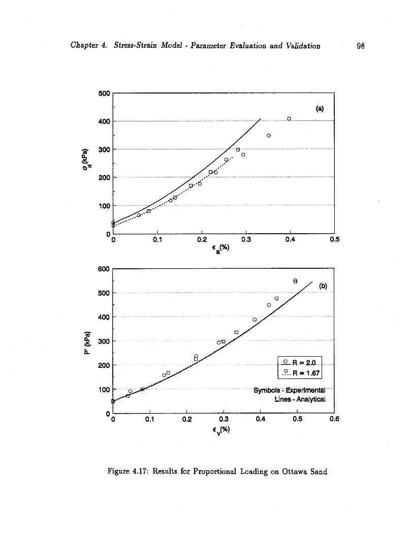
Chapter 4. Stress-Strain Model - Parameter Evaluation and Validation
500
400
3000
200
100
600
500
400
0
a-
200
100
00
98
1.67
Symbols - ExperIment
Lines - AnaIytca1
I_ —— I I
0.1 0.2 0.3 0.4 0.5 0.6
Figure 4.17: Results for Proportional Loading on Ottawa Sand
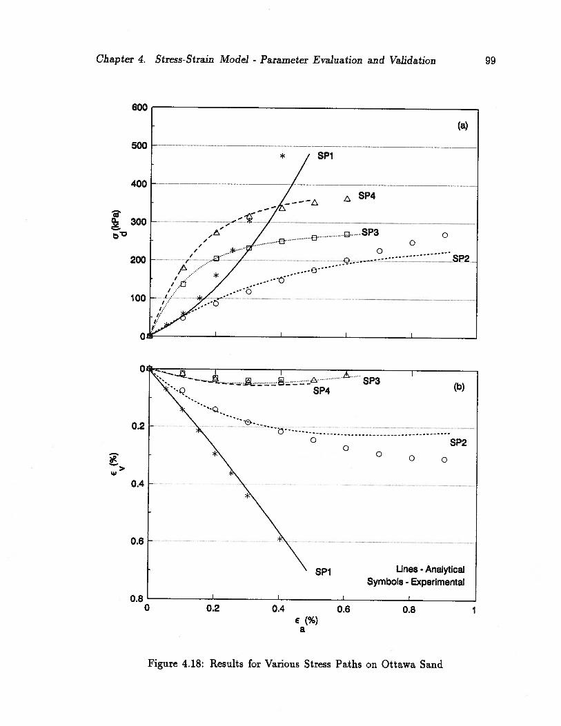
Chapter 4. Stress-Strain Model - Parameter Evaluation and Validation 99
600
500
400
300
200
100
>iLl
0.4
0.6
0.8
0.2
a
0 0.2 0.4 0.6 0.8 1
Figure 4.18: Results for Various Stress Paths on Ottawa Sand

Chapter 4. Stress-Strain Model - Parameter Evaluation and Validation 100
>
E=
100
80
60
40
20
010.0
I I I I I 111111 I I -__
UTF Sand4
• Other McMurray - — —
Sands: - coarse I 1- medium -—— I-fine
.:::ZE
.--——
1.0 milhimetet 0.1 0.01
I I0.1 . 0.01 0.001
inches
I F F Fl F I F F F F I8 12 18 25 35 45 60 80 120 170 230 325400
U.S. mesh
Figure 4.19: Grain Size Distribution for Athabasca Oil Sands, (after Edmunds et al.,1987)
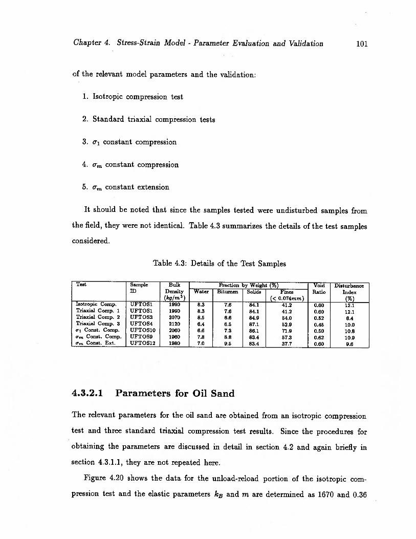
Chapter 4. Stress-Strain Model - Parameter Evaluation and Validation 101
of the relevant model parameters and the validation:
1. Isotropic compression test
2. Standard triaxial compression tests
3. i constant compression
4. U constant compression
0m constant extension
It should be noted that since the samples tested were undisturbed samples from
the field, they were not identical. Table 4.3 summarizes the details of the test samples
considered.
Table 4.3: Details of the Test Samples
Test Sample Bulk Fraction by Weight (%) Void DisturbanceID Density Water Bitumen Solids Fines Ratio Index
(kg/rn3) (< 0.074rnrn) (%)Isotropic Comp. UFTOS1 1990 8.3 7.6 84.1 41.2 0.60 12.1Triaxial Comp. 1 UFTOS1 1990 8.3 7.6 84.1 41.2 0.60 12.1Triaxial Comp. 2 UFTOS3 2070 8.5 6.6 84.9 54.0 0.52 6.4Triaxial Comp. 3 UFTOS4 2120 6.4 6.5 87.1 52.9 0.45 10.00.1 Const. Comp. UFTOS1O 2060 6.6 7.3 86.1 71.9 0.50 10.80m Const. Comp. UFTOS9 1960 7.8 8.8 83.4 57.3 0.62 10.90m Const. Ext. UFTOS12 1980 7.0 9.5 83.4 37.7 0.60 9.6
4.3.2.1 Parameters for Oil Sand
The relevant parameters for the oil sand are obtained from an isotropic compression
test and three standard triaxial compression test results. Since the procedures for
obtaining the parameters are discussed in detail in section 4.2 and again briefly in
section 4.3.1.1, they are not repeated here.
Figure 4.20 shows the data for the unload-reload portion of the isotropic com
pression test and the elastic parameters kB and m are determined as 1670 and 0.36
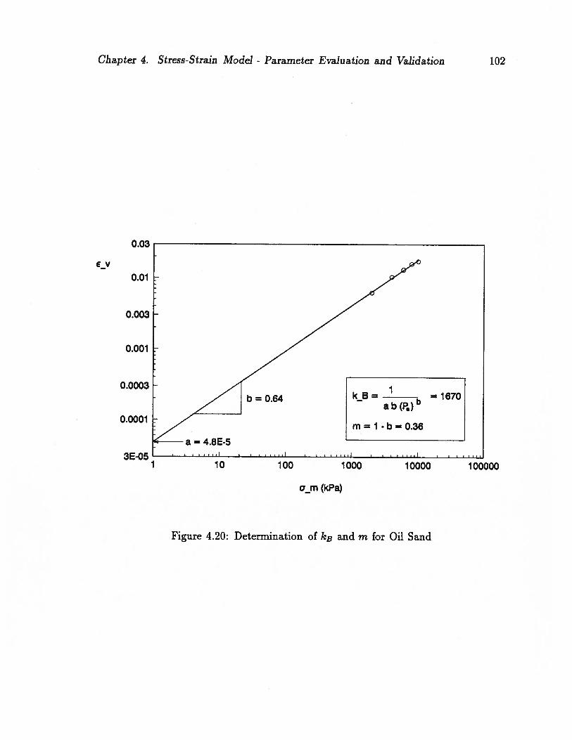
Chapter 4. Stress-Strain Model - Parameter Evaluation and Validation 102
0.03
EV
0.01
0.003
0.001
0.0003
0.0001
3E-051 10 100 1000 10000
am (kPa)
100000
Figure 4.20: Determination of kB and m for Oil Sand

Chapter 4. Stress-Strain Model - Parameter Evaluation and Validation 103
respectively. The Poisson ratio is assumed to be 0.2 and kE and n are determined as
3000 and 0.36. The plastic collapse parameters C and p are obtained from the primary
loading portion of the isotropic compression test as 0.00064 and 0.61 respectively (see
figure 4.21).
/ a
1
0.3
0.1
0.03
0.01
0.003
0.001
0.0003
The failure and hardening rule parameters are obtained from the triaxial com
pression tests as explained in section 4.2.3. Figure 4.22 shows the relevant graph to
obtain the failure parameters. The hardening rule parameters are obtained as shown
in figure 4.23.
The reduced data to obtain the flow rule parameters are shown in figure 4.24. The
results from the three triaxial tests do not seem to give a unique set of parameters as
observed in Ottawa sand. This can be attributed to the differences in field samples.
It is evident from figure 4.24(a) that different flow rule parameters can be obtained
1 10 100 1000 10000 100000
Figure 4.21: Plastic Collapse Parameters for Oil Sand
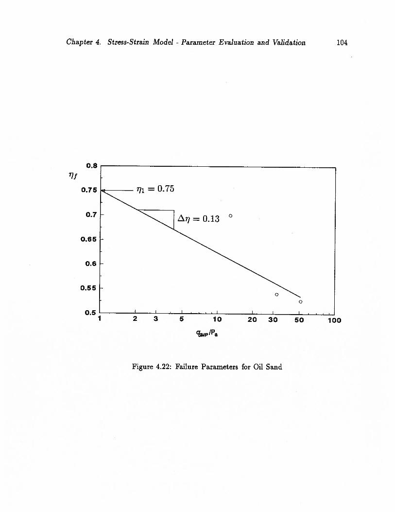
104Chapter 4. Stress-Strain Model - Parameter Evaluation and Validation
0.8
1f
0.75
0.7
0.65
06
0.55
0.5I 2 3 5 10 20 30 50
Mp’a
100
Figure 4.22: Failure Parameters for Oil Sand

Chapter 4. Stress-Strain Model - Parameter Evaluation and Validation 105
2000
1300
1000 -
500-
= -0.66
2000
0
100 -
0
50 I
1 2 3 5 10 20 30 50 100
MP’a
Figure 4.23: Determination of K0 and np for Oil Sand

Chapter 4. Stress-Strain Model - Parameter Evaluation and Validation 106
0.8
0.7
0.6
0.5
0.4
0.3
0.2
0.1
0.4
0-0.4
7,EJ
A
0 --./- .------
0.2 0.4
o.9
0.6 0.8
(a)11
0.8
0.7
0,6
0.5
0—-0.4 -0.2
o a_3=1.OMPa
o _3 = 2.5 MPa
c,_3 = 4.0 MPa
0
—(dEsMp/d7sMP)
0.3
0.2
0.1
-0.2 0 0.2 0.4 0.6
—(dEsMp/d7sMP)0.8
Figure 4.24: Flow Rule Parameters for Oil Sand

Chapter 4. Stress-Strain Model - Parameter Evaluation and Validation 107
if the individual test results are considered. However, an average set of parameters
can be obtained as shown in figure 4.24(b). The flow rule parameters are very much
governed by the volumetric strain behaviour and this will be discussed more in section
4.3.2.2. The summary of the parameters obtained for oil sand is given in table 4.4.
Table 4.4: Soil Parameters for Oil Sand
Elastic kE 3000n 0.36
kB 1670m 0.36
Plastic Shear 0.75iii 0.13\ 0.53ii 0.31
KG 1300rip -0.66R1 0.73
Plastic Collapse C 0.00064
p 0.61
4.3.2.2 Validation
Figure 4.25 shows the experimental and predicted results for loading and unloading of
the isotropic compression test. It can be seen that the results are in good agreement.
Figure 4.26 shows the experimental and predicted results for the triaxial compres
sion tests. It can be seen that the predicted and measured deviator stress versus axial
strain agree very well. The volumetric strain versus axial strain agree reasonably well
for 03 = 1.OMPa and O = 2.5MPa but not for o = 4.OMPa. This is because
the selected flow rule parameters are the average parameters and they tend to agree
closely with those two tests. It can be seen from figure 4.24 that for 03 = 4.OMPa, the
straight line relation is much different and steeper, which would have given a higher

Chapter 4. Stress-Strain Model - Parameter Evaluation and Validation 108
14000
12000 - 0
10000 -
8000 - Loading
b 6000 -
Unloading
4000- 0
2000 o Line - PredictedSymbols - Measured
0I I I I
0 0.5 1 1.5 2 2.5 3
LV (%)
Figure 4.25: Results for Isotropic Compression Test on Oil Sand
Chapter 4. Stress-Strain Model - Parameter Evaluation and Validation 109
value of ). As the line becomes steeper, there will be less volumetric expansion and
the overall behaviour will be more contractive. If a higher value of ) is selected, the
predictions and observations would agree well for o 4.OMPa. It is also interesting
to note that the value of the flow rule parameter i is not much different for the three
tests. The value of .t is, in fact, an indication of ultimate stress ratio or a state of
shearing with constant volume.
Results for three different stress paths; constant o, compression, constant °m
compression and constant om extension are shown in figure 4.27. The stress paths
are shown in the insert of the figure. It can be seen that the experimental and
predicted results are in good agreement.
4.4 Sensitivity Analyses of the Parameters
In order to provide a better understanding about the significance of the parameters,
sensitivity analyses on the parameters have been carried out. The parameters ob
tained for Ottawa sand were chosen as the base parameters and the significance of a
particular parameter was studied by changing only that parameter. A triaxial com
pression loading condition with the initial confining stress of 500 kPa was considered
and the results in terms of deviator stress and volumetric strain are analyzed. The
results are shown in figures 4.28 and 4.29
The plastic collapse parameters C and p are essentially an indication of isotropic
compressibility. The higher the values, the higher the predicted volumetric strains.
The parameter ). is the slope of the flow rule and it defines the change in volumetric
expansion for a change in stress ratio. A steeper slope (or higher A) will give less
volumetric expansion. The parameter 1u is the amount of stress ratio which separate
contraction and dilation (similar to ç5 in general soil mechanics). A smaller value of
will result in dilation at lower stress ratio.
The parameters KG and np define the initial slope of the hardening modulus
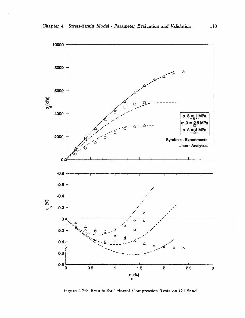
Chapter 4. Stress-Strain Model - Parameter Evaluation and Validation 110
0
>w
10000 -
8000 -
6000 -
4000
2000
0
0.2
0.4
0.6
0.8
--: :
MPa
a_3 =.5 MPa
a_3=,MPa
Symbols - Experimental
Lines - Analytical
-0.8
-0.6
-0.4
-0.2
0 0.5 1 1.5 2 2.5 3
e(%)a
Figure 4.26: Results for Triaxial Compression Tests on Oil Sand
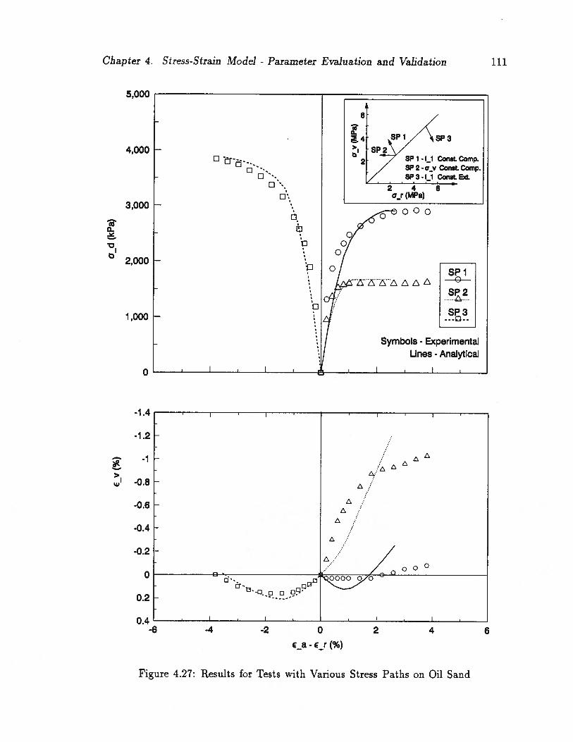
Chapter 4. Stress-Strain Model - Parameter Evaluation and Validation 111
5,000 —
4,000 -
3,000 -
2,000
1,000
0
6
-4
I
/ SP1-I.1 Const.Comp2 / SP 2- a_v Const Comp./ SP3-i1 Conet Ext.
246a_r (MPa)
D.C-..
C’-,
I1
‘a
a
&
>WI
000
or0/
0/
______
o/ spiC
SP3
Symbols- Experimental
Lines - Analytical
-1.4
-1.2
—1
-0.8
-0.6
-0.4
-0.2
0
0.2
0.4
zgD Q9OO5/O
. -ci - o o
-6 -4 -2 0 2 4 6- E_r (%)
Figure 4.27: Results for Tests with Various Stress Paths on Oil Sand

Chapter 4. Stress-Strain Model - Parameter Evaluation and Validation
Ea (%)
(C) Effect of Parameter A
0
0
&
112
c_a (%) c_a (%)
(a) Effect of Parameter C (b) Effect of Parameter p
I
>WI
0.4 0.6 0.8 1
c_a (%)
(d) Effect of Parameter L
Figure 4.28: Sensitivity of Parameters C,p, ) and i
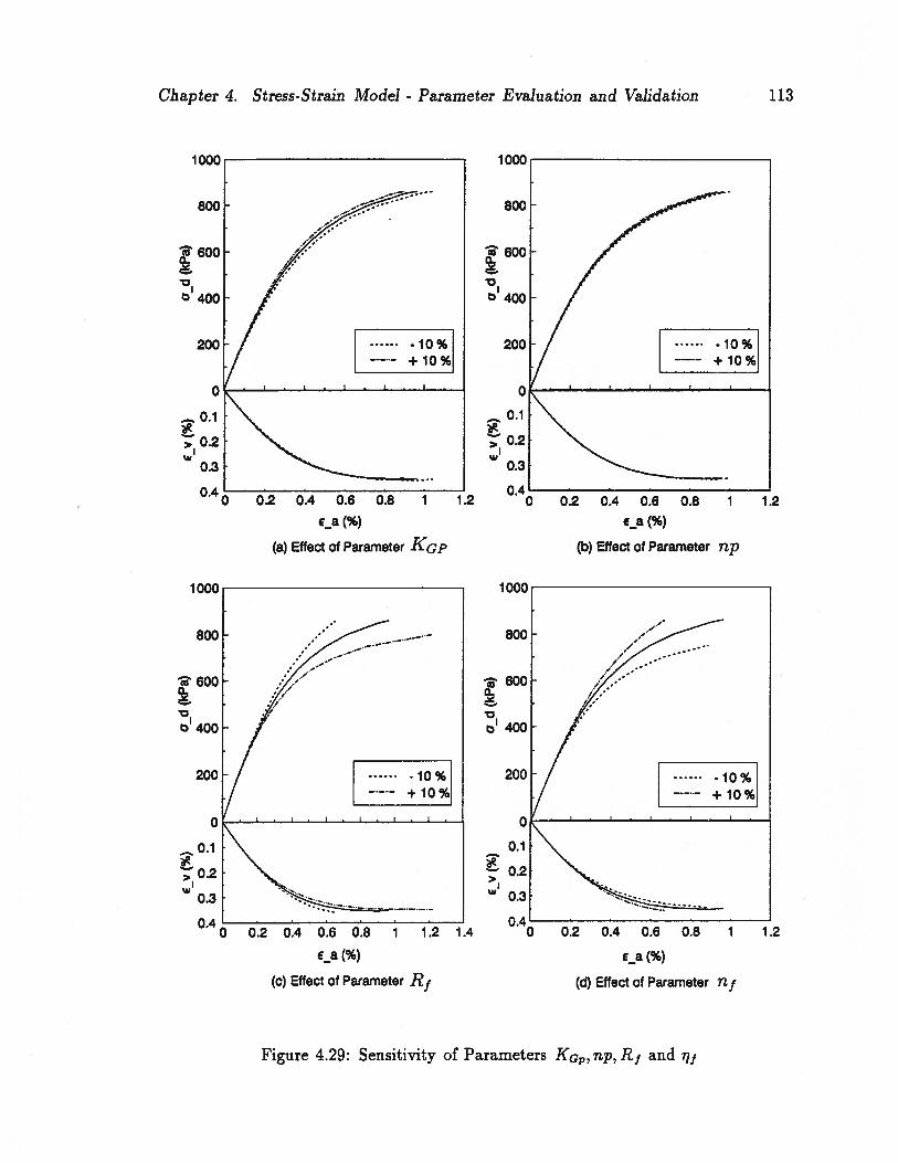
Chapter 4. Stress-Strain Model - Parameter Evaluation and Validation 113
(c) Effect of Parameter Rf
1.2
€_a (%) E_a (%)
(a) Effect of Parameter KGp (b) Effect of Parameter rip
0
&
Ea (%) c_a (%)
(d) Effect of Parameter flf
Figure 4.29: Sensitivity of Parameters KG, np, R1 and i
Chapter 4. Stress-Strain Model - Parameter Evaluation and Validation 114
G,. A higher value of will result in a stiffer deviator stress response and a lower
volumetric strain response. The parameter R1 and i define the shape and the failure
stress ratio in the hardening rule. Lower R1 and higher i will give stiffer deviator
stress response.
The elastic parameters are not considered here because they have been widely
used and their significance is well understood.
4.5 Summary
A double hardening elasto-plastic model has been postulated to model the stress-
strain behaviour of oil sands. Procedures for the evaluation of the parameters and
the validation of the proposed model have been presented in this chapter.
The model parameters are relatively easy to obtain and can be determined from
conventional isotropic and triaxial compression test results. The parameters have
physical meanings and a sensitivity study has been carried out on the parameters to
better explain their physical significance. Laboratory test results for various stress
paths have been compared with the model predictions. Measured results and predic
tions agree very well and the model predicts the shear induced dilation effectively.
From the validations presented in this chapter, it can be concluded that the proposed
model captures the stress-strain behaviour of oil sands very well.
Chapter 5
Flow Continuity Equation
5.1 Introduction
The pore fluid in the oil sand matrix comprises three phases namely gas, oil and water
and therefore, the fluid flow phenomenon is of multi-phase nature. In petroleum
reservoir engineering, the flow in oil sand is often analyzed as multi-phase flow, but
solely as a flow problem without paying much attention to the porous medium. The
most widely used model to analyze the flow in oil sand is called ‘3-model’ or ‘the
black-oil model’ (Aziz and Settari, 1979) and it makes the following assumptions.
1. There are three distinct phases; oil, water and gas.
2. Water and oil are immiscible and they do not exchange mass or phases.
3. Gas is assumed to be soluble in oil but not in water.
4. Gas obeys the universal gas law.
5. Gas exsolution occurs instantaneously.
With these assumptions, and considering the effects of stresses and temperature
changes in the sand skeleton, a flow continuity equation is derived in this chapter
from the general equation of mass conservation. However, the flow equations are not
considered separately for individual phases as in petroleum reservoir engineering. All
three flow equations are combined and a single effective equation is formulated. In
essence, the derived flow continuity equation is similar to a single phase flow equation
115
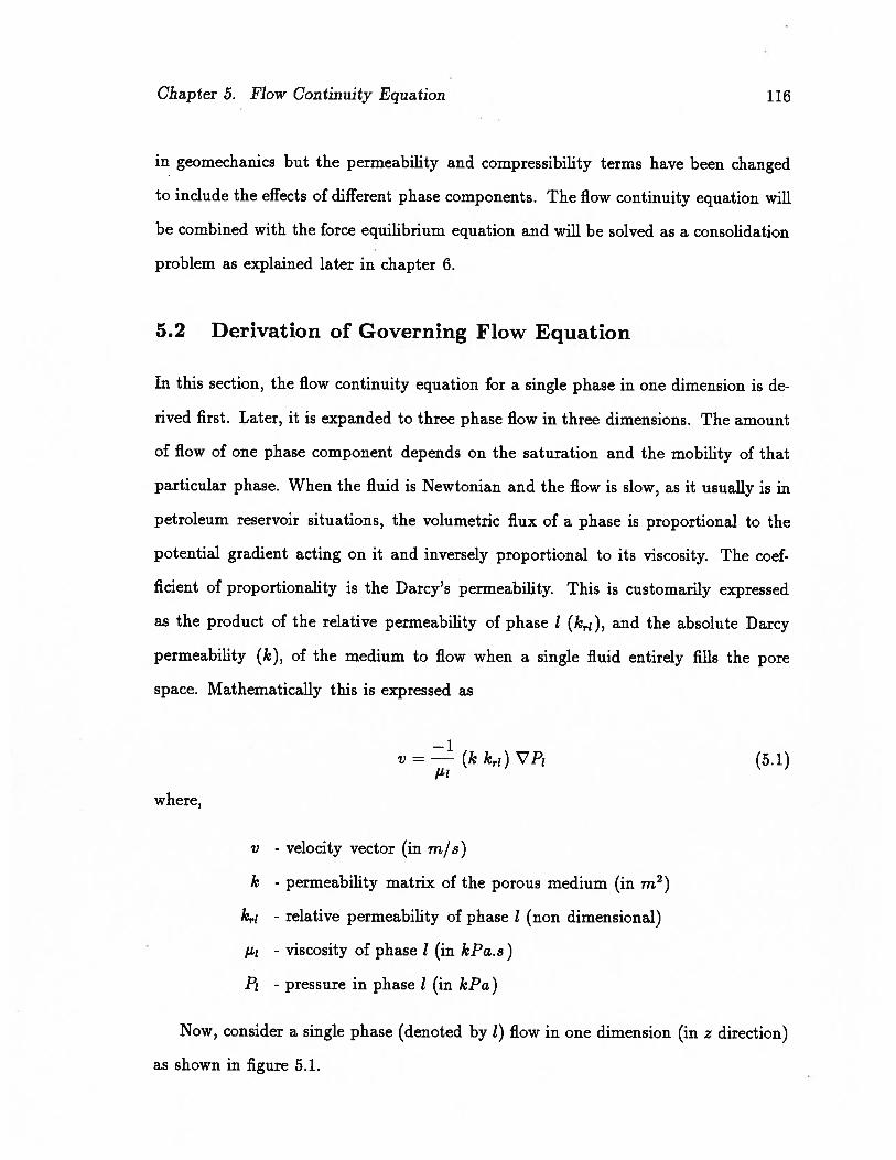
Chapter 5. Flow Continuity Equation 116
in geomechanics but the permeability and compressibility terms have been changed
to include the effects of different phase components. The flow continuity equation will
be combined with the force equilibrium equation and will be solved as a consolidation
problem as explained later in chapter 6.
5.2 Derivation of Governing Flow Equation
In this section, the flow continuity equation for a single phase in one dimension is de
rived first. Later, it is expanded to three phase flow in three dimensions. The amount
of flow of one phase component depends on the saturation and the mobility of that
particular phase. When the fluid is Newtonian and the flow is slow, as it usually is in
petroleum reservoir situations, the volumetric flux of a phase is proportional to the
potential gradient acting on it and inversely proportional to its viscosity. The coef
ficient of proportionality is the Darcy’s permeability. This is customarily expressed
as the product of the relative permeability of phase 1 (krj), and the absolute Darcy
permeability (k), of the medium to flow when a single fluid entirely fills the pore
space. Mathematically this is expressed as
VP1 (5.1)
where,
v - velocity vector (in m/s)
k - permeability matrix of the porous medium (in m2)
krt - relative permeability of phase 1 (non dimensional)
I’i - viscosity of phase 1 (in kPa.s)
P1 - pressure in phase 1 (in kPa)
Now, consider a single phase (denoted by 1) flow in one dimension (in z direction)
as shown in figure 5.1.

Chapter 5. Flow Continuity Equation
n - porosityS1 - saturation of phase 1
- velocity of phase 1 in z direction- unit weight of phase I
117
0(vj 71) dzôz
S1ndzn dz
dz
Phase ‘I’ in pore fluid
Pore fluid
— Solids
I
Figure 5.1: One dimensional flow of a single phase in an element

Chapter 5. Flow Continuity Equation 118
Weight of phase 1;
wi=nSi7jdz (5.2)
Incoming mass flux:
v yi (5.3)
Outgoing mass flux:
= + dz (5.4)
Difference between flux coming in and flux going out:
QI_Qo_O(vZz_y1)d 55dt 8z (.)
Rate of storage:
&wlO(nSl7l)d 568t ôt
For conservation of mass, the difference between the incoming and outgoing flux
should be equal to the rate of storage. Thus,
— O(vi 71) — 8(n Si 7i) 5 78z — ôt (.)
Expansion of the partial differentials in equation 5.7 gives
avzl 871 8n &Y1 8S1—7z—+v2i—=7iSi+nSi--+n7i-- (5.8)
Dividing by 7i yields
8v21 v21 871 8m S1 871 8S1——+----—-—=Si——+n—-—+n------ (5.9)
8z 71 8z 7’ at at
Now, consider all five terms in equation 5.9 separately, starting from the left hand
side.
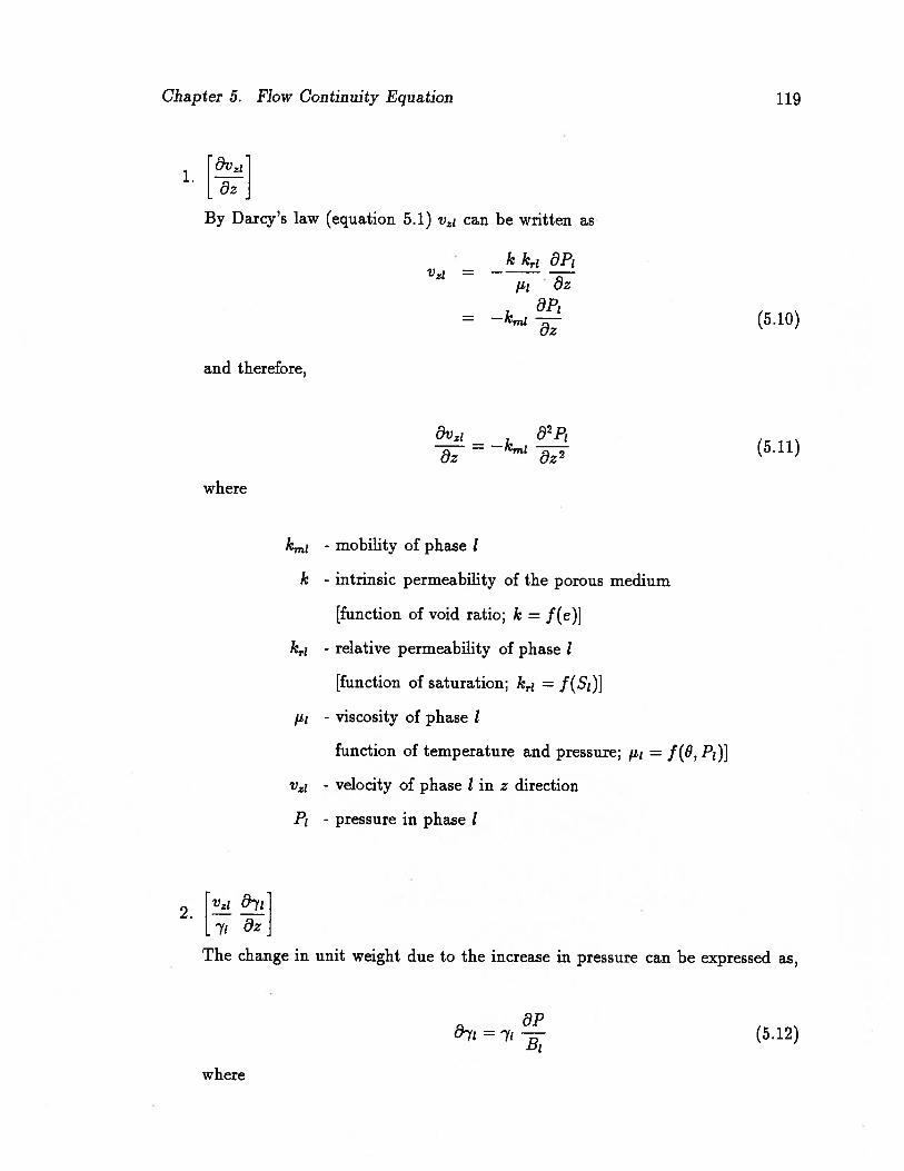
Chapter 5. Flow Continuity Equation 119
0v218z
By Darcy’s law (equation 5.1) v can be written as
kkr 8P1vz1 = —
____
—
ILl c9z
= (5.10)
and therefore,
92P1= (5.11)
where
kmi - mobility of phase 1
k - intrinsic permeability of the porous medium
[function of void ratio; k = f(e)]
k,.1 - relative permeability of phase 1
[function of saturation; k,.1 = f(S1)]
- viscosity of phase 1
function of temperature and pressure; = f(8, F1)]
vz - velocity of phase 1 in z direction
P1 - pressure in phase 1
271 8z
The change in unit weight due to the increase in pressure can be expressed as,
871 = 71 (5.12)
where
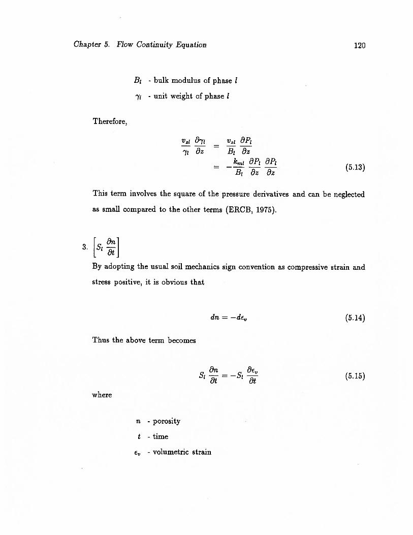
Chapter 5. Flow Continuity Equation 120
B1 - bulk modulus of phase 1
- unit weight of phase 1
Therefore,
87j — v
yi 8z — B1 öz— kmi 6P1
5 13— B1 8z 8z
This term involves the square of the pressure derivatives and can be neglected
as small compared to the other terms (ERCB, 1975).
3. S1--
By adopting the usual soil mechanics sign convention as compressive strain and
stress positive, it is obvious that
dm = —dEn (5.14)
Thus the above term becomes
(5.15)
where
n - porosity
t -time
- volumetric strain

Chapter 5. Flow Continuity Equation 121
S1 b-y.4. n—-—
7i ôt
By using equation 5.12 this term can be written as,
51 87j 51 8P1(5.16)
718t B18t
as1.
Summation of saturations of all phase components should always be equal to
unity. Hence, when combining the equations for all the phases, the summation of
this term over all the phases will be zero. Mathematically this can be expressed
as
(5.17)
Since the final equation is to be derived by combining all the phases this term
need not to be considered in detail.
By making the changes to the terms as explained so far, equation 5.9 can be
written as
82P s1 8P1 8Sikmi -ä—-H-S1 --—n- --—n--O (5.18)
Extension of equation 5.18 to three dimensions yields
kmiV2Pi + 51L — — = 0 (5.19)

Chapter 5. Flow Continuity Equation 122
where
2 b’P ElF t92p(5.20)
Hence, the equations of flow for the three phases in oil sand, in three dimensions,
will be as follow:
for water phase;
(5.21)
for oil phase;
kmo V2P0H-50a
—ns0 ap0
—n = 0 (5.22)
for gas phase;
kmg V2P9 + S9 — — n = 0 (5.23)
where,
km - mobility
S - saturation
B - bulk modulus
and subscripts o, w and g denote oil, water and gas respectively. It should be noted
that in the formulation the capillary pressure between two phases is assumed to be
constant for the increment and therefore, it will not appear in derivatives.
Combining equations 5.21, 5.22 and 5.23 gives
(kmo+kmw+kmg) V2p+_n (++) =0 (5.24)
This can be written as
Chapter 5. Flow Continuity Equation 123
2 OPkEQ V P + — CEQ -- = 0 (5.25)
where,
kEQ - equivalent hydraulic conductivity
= kmo + kmw + kmg
CEQ - equivalent compressibility— (S0 Sw Sg
Equation 5.25 is similar to the one used by Vaziri (1986) and Srithar (1989), except
for the equivalent conductivity term. They considered the contributions from different
fluid phase components in the compressibility but not in the hydraulic conductivity.
Recently, Settari et al. (1993) have also used an effective hydraulic conductivity term
to model the three-phase fluid which is similar to the equivalent hydraulic conductivity
term derived above. The equivalent hydraulic conductivity is a function of mobilities
of the phases which in turn depend on their relative permeabilities and viscosities.
Evaluations of relative permeabilities and viscosities are described in detail in the next
sections. The equivalent compressibility is a function of saturation and bulk modulus
of individual phase components and the details of its evaluation are described in
section 5.5.
5.3 Permeability of the Porous Medium
The permeability of the porous medium (k) mainly depends on the amount of void
space. Lambe and Whitman (1969) collected considerable experimental data to study
the variation of k with void ratio. Although there was a considerable scatter in the
data, they found that there is a linear relationship between k and a void ratio function
e3/(1 + e) for a wide range of granular materials. It can be argued that various other
relationships could be established for the varition of k with e. However, without the

Chapter 5. Flow Continuity Equation 124
need for much specific details about the soil, the relationship given by Lambe and
Whitman (1969) is quite reasonable for most engineering purposes. Using Lambe and
Whitman’s relationship, at a particular void ratio of e, k can be expressed as
k =kOe/(l±e) (5.26)e/(1 + eo)
where e0 and k0 are the initial void ratio and the initial permeability of the porous
medium respectively.
5.4 Evaluation of Relative Permeabilities
Measurement of three-phase relative permeability in the laboratory is a difficult and
time consuming task. Due to the complications associated with the three-phase flow
experiments, empirical models have been used extensively in the reservoir simulation
studies. These models use two sets of two-phase experimental data to predict the
three-phase relative permeabilities. Figure 5.2 shows typical results that might be
obtained for such two-phase systems. Figure 5.2(a) shows the relative permeability
variations for an oil-water system and figure 5.2(b) shows the relative permeability
variations for a gas-oil system.
Numerous experimental studies on relative permeabilities have been reported
in the petroleum reservoir engineering literature starting from Leverett and Lewis
(1941). Many review articles have also appeared in the literature (Saraf and McCaf
fery (1981), Parameswar and Maerefat (1986), Baker (1988)) and an assessment of
these studies is beyond the scope of this thesis. However, the general conclusion from
these studies suggests that the functional dependence of relative permeabilities can
be given by
= f(S)
krg = f(S9)
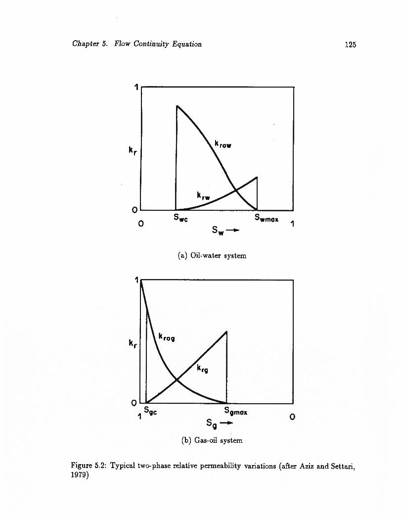
Chapter 5. Flow Continuity Equation 125
0
krow
k,,,
(b) Gas-oil system
Figure 5.2: Typical two-phase relative permeability variations (after Aziz and Settari,1979)
I
kr
0
I
kr
0Swmaz
SW—,’..
(a) Oil-water system
rg_
ISgc Sgmoz
Sg0

Chapter 5. Flow Continuity Equation 126
k,.0 = f(S0) (5.27)
The function for the relative permeability of oil, k,.0, is not readily known and it
is estimated from the two-phase data for k,., and k,.09, where, k,.OW is the relative
permeability of oil in an oil-water system and k,.09 is the relative permeability of oil
in an oil-gas system. Their functional dependence are given by
k,.0 = f(SW)
k,.09 = f(S9) (5.28)
The simplest way of estimating k,.0 would be,
k,.0 = k,.0 k,.09 (5.29)
Two more accurate models have been proposed by Stone (1970), only the first of
which is considered here. In this model, Stone (1970) defines normalized saturations
as
S= —
S S (5.30)wc om
= SO SomSo Sam (5.31)
wc om
5;= 15S95
(5.32)wc am
Where, S, is called the critical or connate water saturation at which water starts
to flow. When S,, is less than S, the relative permeability of water k,., will be zero.
Sam is called the residual oil saturation at which oil ceases to flow when it displaced
simultaneously by water and gas. If S is less than 5om, k,.0 will be zero.
According to Stone (1970), the relative permeability of oil in a three-phase system
is given by
k,.0 = S (5.33)

Chapter 5. Flow Continuity Equation 127
The factors i3 and ,i3 are determined from the end conditions that equation 5.33
should match the two-phase data at the extreme points. The two extreme cases of
= 0 and SL, = give
— 1 — S
k,.09— 1 — S’9
(5.34)
(5.35)
The region of mobile oil phase (i.e. k,.0 > 0) predicted by Stone’s model I is shown
in figure 5.3 on the ternary diagram assuming increasing 5W and S9. For conditions
depicted by point outside the hatched area, the relative permeability of oil will be
zero.
100%WATER
Figure 5.3: Zone of mobile oil for three-phase flow (after Aziz and Settari, 1979)
100%GASE1S Som
I,. 100%OIL
Aziz and Settari (1979) modified Stone’s model because Stone’s model will reduce

Chapter 5. Flow Continuity Equation 128
exactly to two-phase data only if the relative permeabilities at the end points are
equal to one, i.e., krow(Swc) = krog(Sg = 0) = 1. They suggest that the oil-gas data
has to be measured in the presence of connate water saturation. In that case, an oil-
water system at S, and an oil-gas system at S = 0 are physically identical. Both
systems will have, S = S and S0 = 1 — S at 59 = 0. At these conditions, the
relative permeabilities will be
krow(Swc) = krog(Sg = 0) = krocw (5.36)
Then, the modified form of Stone’s equations will be
k,.0 = S krocw w /39 (5.37)
k— (5.38)
—
k,.0911 c’ (. )
,.0cwI — LI9
Kokal and Maini (1990) claim that Aziz and Settari’s method has problems be
cause:
1. Measurements of two-phase oil-gas data are not necessarily obtained at connate
water saturation
2. The relative permeability at connate water saturation in an oil-water system
generally will not be equal to that in an oil-gas system
Kokal and Maini (1990) further modified Stone’s model by incorporating another
normalizing factor. After these modifications, the relevant equations needed to predict
the relative permeability of oil are
Chapter 5. Flow Continuity Equation 129
k,.0 = s (k,?09S;+k,?,&S)(5.40)
rOW4wko(1SI
a rog“9k0 (1Srog\ g
where,
k,?0 - relative permeability of oil at connate water saturation
in a water-oil system
k,?09 - relative permeability of oil at zero gas saturation
in an oil-gas system
When k,?0 = k,?og, the above model reduces to the one given by Aziz and Settari
(1979). Kokal and Maini (1990) compared model predictions against measured data
and found very good agreement. The best comparison given in their paper is shown
in figure 5.4.
From the discussion so far in this section, it can be concluded that the relative
permeabilities in three-phase system can be written as
= f(S) (5.43)
k,.9 = f(S9) (5.44)
k,.0 = f(k,.0,k,.09, Sw, so, S) (5.45)
k,.0 = f(5) (5.46)

Chapter 5. Flow Continuity Equation 130
OILExpenmental
— Calculated0.75
0.70
0.60
0.50
0.40
0.30020
0.100.01
. . ..
WATER “ “ “ “ ‘.‘ “ ‘I’ ‘ GAS
Figure 5.4: Comparison of calculated and experimental three-phase oil relative permeability (after Kokal and Maini, 1990)
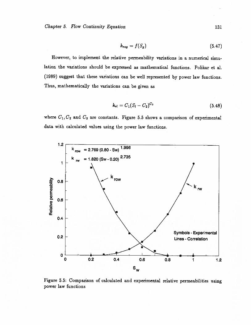
Chapter 5. Flow Continuity Equation 131
a)Ea,a)>
a)
— f(S9) (5.47)
However, to implement the relative permeability variations in a numerical simu
lation the variations should be expressed as mathematical functions. Polikar et al.
(1989) suggest that these variations can be well represented by power law functions.
Thus, mathematically the variations can be given as
= C1(S1 — C2)c3 (5.48)
where C1,C2 and C3 are constants. Figure 5.5 shows a comparison of experimental
data with calculated values using the power law functions.
1.2k = 2.769 (0.80 - Sw) 1.996
k = 1.820 (Sw - 0.20) 2.735
row
1
0.8
0.6
0.4
0.2
0
‘ k rw
Symbols- ExperimentalLines - Correlation
0 0.2 0.4 0.6 0.8
w
1 1.2
Figure 5.5: Comparison of calculated and experimental relative permeabilities usingpower law functions
Chapter 5. Flow Continuity Equation 132
In summary, the relevant parameters needed to calculate the relative permeabil
ities of water, oil and gas phases are given in table 5.1. An example showing the
details of the calculations of the relative permeabilities and the resulting equivalent
permeability is given in appendix B, to provide a better understanding of the steps
involved.
5.5 Viscosity of the Pore Fluid Components
5.5.1 Viscosity of Oil
The mobility of an individual phase in a three-phase system depends on the viscosity
of the phase component. Viscosities of the fluid components are generally strong
functions of temperature and to some extent depend on the pressure as well.
Viscosity of oil plays a very important role in reservoir engineering. Crude oil
cannot flow at the ambient temperatures because of its high viscosity. The oil recovery
methods require some form of heating to reduce the viscosity and thereby increase
mobility. For example, the viscosity of Cold Lake bitumen is 20, 000 mPa.s at 30°C
and 100 mPa.s at 100°C, i.e., a 200-fold reduction at high temperature. There are
some correlations for the viscosity of oil available in the literature. Among those
correlations, the one proposed by Puttagunta et al. (1988) has been selected in this
study for the following reasons:
1. It requires only a single viscosity value at 30°C and 1 atmosphere as input data.
2. Generally, oil viscosity varies widely from deposit to deposit and this correlation
fits the viscosity variation of most bitumens reasonably well.
The correlation proposed by Puttaguntta et al. (1988) is expressed by the follow
ing equation:
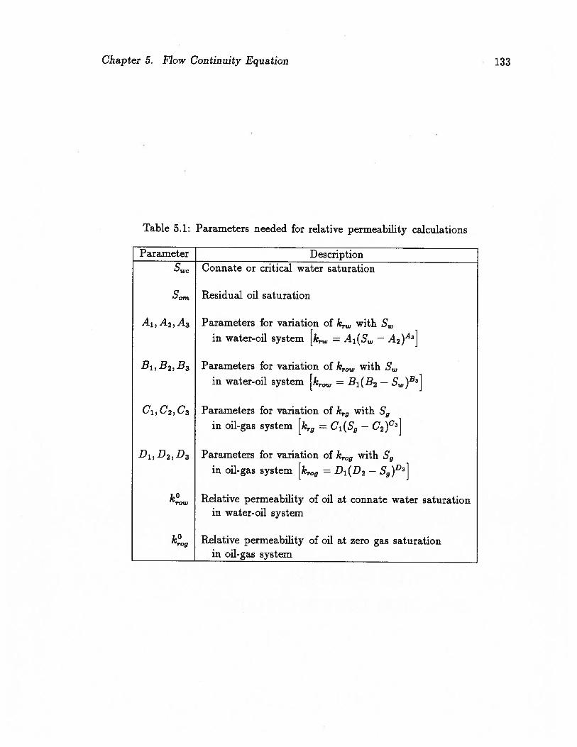
Chapter 5. Flow Continuity Equation 133
Table 5.1: Parameters needed for relative permeability calculations
Parameter DescriptionConnate or critical water saturation
Som Residual oil saturation
A1,A2,A3 Parameters for variation of k with Si,,in water-oil system = A1(S — A2)A3]
B1,B2,B3 Parameters for variation of krow with 5win water-oil system [kro B1(B2 — Sw)B3]
C1,C2,C3 Parameters for variation of krg with Sgin oil-gas system [krg = C1(S9 — C2)c3]
D1,D2,D3 Parameters for variation of krog with S9in oil-gas system [k.09 = D1(D2— 59)D3]
Relative permeability of oil at connate water saturationin water-oil system
k,?09 Relative permeability of oil at zero gas saturationin oil-gas system
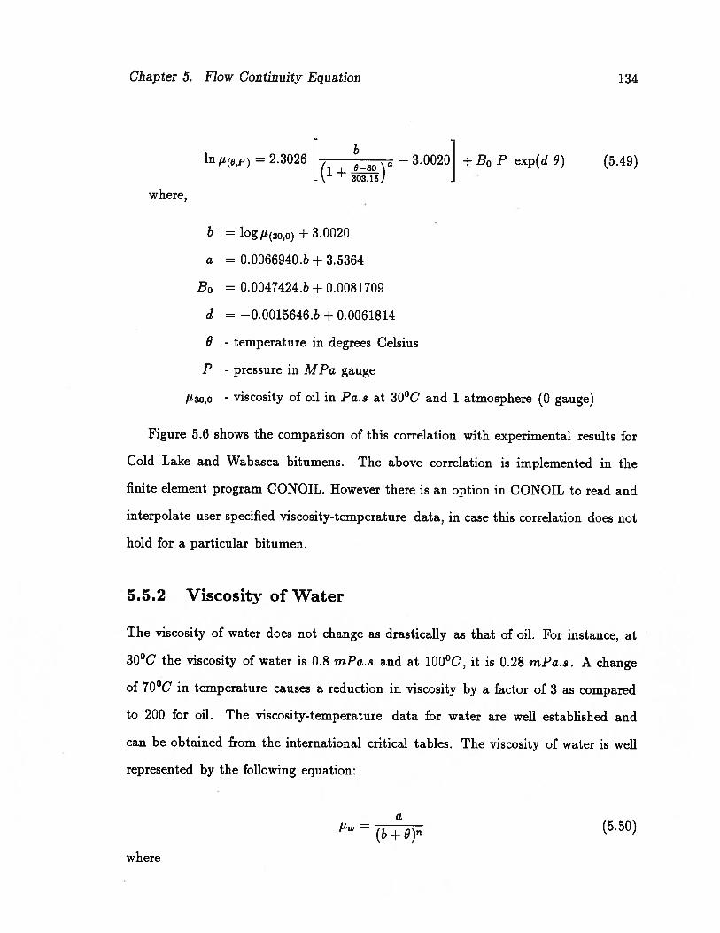
Chapter 5. Flow Continuity Equation 134
lfl(9,p) 2.3026( 8-30
— 3.0020] + B0 F exp(d 6) (5.49)+ 30315)
where,
b log .Lt(3o,o) + 3.0020
a = 0.0066940.b + 3.5364
B0 = 0.0047424.b + 0.0081709
d = —0.0015646.b + 0.0061814
8 - temperature in degrees Celsius
F - pressure in MFa gauge
- viscosity of oil in Fa.s at 30°C and 1 atmosphere (0 gauge)
Figure 5.6 shows the comparison of this correlation with experimental results for
Cold Lake and Wabasca bitumens. The above correlation is implemented in the
finite element program CONOIL. However there is an option in CONOIL to read and
interpolate user specified viscosity-temperature data, in case this correlation does not
hold for a particular bitumen.
5.5.2 Viscosity of Water
The viscosity of water does not change as drastically as that of oil. For instance, at
30°C the viscosity of water is 0.8 mPa.s and at 100°C, it is 0.28 mFa.s. A change
of 70°C in temperature causes a reduction in viscosity by a factor of 3 as compared
to 200 for oil. The viscosity-temperature data for water are well established and
can be obtained from the international critical tables. The viscosity of water is well
represented by the following equation:
= (b+8)(5.50)
where

Chapter 5. Flow Continuity Equation 135
50000
— empirical equation- * experimental
10000 -
‘‘500o *
SC0SI 1000TY 500
mPa
100S
50. *
10
0 20 40 50 80 100 120
TEEATUR.E, C
a) Wabasca bitumen
50000 -
\ — empirical equation* experimental
10000
VI 5000 -
SCo
4iooo.
500
P
• 100 -
so
10 I I
23 40 50 80 100 120 140
TE’ERATURE, C
b) Cold Lake bitumen
Figure 5.6: Experimental and predicted values of viscosity (after Puttagunta et al.,1988)
Chapter 5. Flow Continuity Equation 136
- viscosity of water
- temperature
a, b, n - constants
It is reasonable to assume the water phase in the oil sand will have the same prop
erties. These data from the International Critical Tables are reproduced in appendix
B and built into the computer program CONOIL. There is also an option to read and
interpolate from any other user specified data.
5.5.3 Viscosity of Gas
There is not much information available about the viscosity of gas in the recent
literature in petroleum engineering. Carr et al. (1954) carried out some work on
the viscosity of hydrocarbon gases as a function of pressure and temperature. The
viscosity of gas appears to be equally dependent on pressure and temperature, but the
variations are not very significant. for example, at atmospheric pressure and at 30°C,
the viscosity of paraffin hydrocarbon gases (molecular weight of 70) is 0.007 mPa.s
and at 200°C it is 0.0105 mPa.s, i.e., increases by only a factor of 1.5. The charts
given in Carr et al. (1954) are given in appendix B with an example calculation.
There is no correlation readily available for the data. The viscosity of the gas is
very low and hence its mobility will be very high compared to that of water and oil.
Therefore, it may not be unreasonable to assume a constant viscosity for gas (for
instance, 0.01 mPa.s). However, there is an option available in CONOIL as for water
and oil, to input any other data at the user’s choice.
5.6 Compressibility of the Pore Fluid Components
In the final flow equation derived (equation 5.25), the equivalent compressibility of
the pore fluid is defined as
Chapter 5. Flow Continuity Equation 137
CEQ =(+±) (5.51)
The bulk moduli of the water and oil can be assumed constant, though they
depend slightly on pressure. The important parameter that affects the equivalent
compressibility is the comprssibility of gas. If there is more gas present in the pore
fluid, it will be more compressible. The compressibility of gas can be determined using
the gas laws. The basic gas laws governing the volume and pressure relationships are
Boyle’s law and Henry’s law. According to Boyle’s law, under constant temperature
conditions,
P9V=w9RT (5.52)
where,
P9 - absolute pressure of gas
T - absolute temperature
R - universal gas constant
V, - volume of gas
Wg - weight of gas
Under undrained conditions, the weight of gas does not change and therefore,
equation 5.52 can be written as
(5.53)
where K is a constant.
Gas can be present in both the dissolved and free states. According to Henry’s
law (Sisler et al., 1953); the weight of gas dissolved in a fixed quantity of a liquid,
at constant temperature, is directly proportional to the absolute pressure of the gas
above the solution. Mathematically, this can be written as
Chapter 5. Flow Continuity Equation 138
0 0
(5.54)
where
- weight of dissolved gas
and the superscripts 0 and 1 refer to the initial and final conditions, respectively.
In other words, Henry’s law implies that the volume of dissolved gas in a fixed
quantity of liquid is constant at a constant temperature and at a confining pressure
F, when the volume is measured at F. Thus
Vd9 = H V0 (5.55)
where
H - Henry’s constant, which is temperature dependent and,
over a wide range of pressure, is also pressure dependent
V0 - volume of oil
Since the volume of dissolved gas is constant, free and dissolved gas components
can be combined. Then application of Boyle’s law to the entire volume yields (Fred
lund, 1976)
(5.56)
where V19 is the volume of free gas.
Rearranging the terms yields,
ID1IT? in— rgkVdg + Vf
V19—
0 — Vdg
9
By differentiating equation 5.57,

Chapter 5. Flow Continuity Equation 139
8V P91(Vdg+Vj9)558)8P9° — (Pg0)2
By adopting the sign convention that compression is positive,
1 - (av1/v1)- P(V9+v)559)Bg 8P9° — V°9(P90)2
Now,
Vd9 = ThiS0
TT0V =
=nS
Pg = Pa+F+Pc (5.60)
where,
- saturation of oil
S9 - saturation of gas
n - porosity
- atmospheric pressure
P - pressure in oil
- capillary pressure
By substituting these last expressions into equation 5.59
iP91(HS0+S)561)B9 S(P9°)2 (
Generally, in an incremental procedure the values used are estimated at the be
ginning of the increment. Therefore, from equation 5.61 the value of (S9/B9)at the
beginning of an increment can be given as
59 HS0+59562
BgPa±P+Pc
Chapter 5. Flow Continuity Equation 140
If the capillary effects are neglected (i.e. P = 0), equation 5.62 will be similar
to the one derived by Bishop and Henkel (1957). Equation 5.62 is slightly different
from the equation derived by Vaziri (1986). In Vaziri’s expression capillary pressure
was assumed to be a function of capillary radius and the capillary radius in turn
was assumed to be a function of saturation. He also included a derivative term
of capillary pressure with respect to saturation which is not significant since the
changes in saturation will be very small. In addition, having this derivative term
is inconsistent because, in his formulation to derive the flow equation, the capillary
pressure was assumed constant over an incremental step. The expression given by
equation 5.62 has a practical advantage because, in reservoir engineering, the variation
of capillary pressure with saturation is readily available, whereas the capillary radius,
critical capillary radius and surface tension values which are needed data for Vaziri’s
expression are not readily available. The capillary pressure P can be well represented
by a power function similar to the ones used for relative permeabilities.
= E1(S9 E2)E3 (5.63)
where E1,E2 and E3 are constants.
Therefore, by substituting equation 5.62 in equation 5.51, the equivalent com
pressibility can be written as
S, SL (S9+HS0)CEQ=fl (5.64)
5.7 Incorporation of Temperature Effects
The fluid flow model described so far is for isothermal conditions and does not in
clude temperature effects. The final equation obtained for multiphase flow (equation
5.25) can be considered as an equation of volume compatibility which is derived from

Chapter 5. Flow Continuity Equation 141
the basic equation of conservation of mass. If the temperature effects are included,
equation 5.25 will become (Srithar (1989), Booker and Savvidou (1985))
kEQ V2F + — CEQ + aEQ = 0 (5.65)
where
cEQ - equivalent coefficient of thermal expansion
- temperature
The equivalent coefficient of thermal expansion can be obtained by considering
the coefficients of thermal expansion of the individual soil constituents and their
proportions of the volume, i.e.,
0EQ = a8(1 — n) + nSa + flSoto + flSgQg (5.66)
where subscripts s, w, o and g denote solid, water, oil and gas respectively.
The coefficient of thermal expansion of solids, water and oil can be measured in
the laboratory. The coefficient of thermal expansion of gas can be obtained from the
universal gas law. According to gas law,
Povo Ply1= (5.67)
To evaluate the coefficient of thermal expansion, only the volume change due to
temperature change has to be considered. Thus, by assuming constant pressure
l 80
V0Vl—Vo
_____
= 80(5.68)
By adopting the usual notation
= (5.69)

Chapter 5. Flow Continuity Equation 142
Hence,
a9 = (5.70)
It should be noted that the temperature in the above equation should be absolute
temperature (i.e. in K).
5.8 Discussion
In this chapter, flow continuity equations for individual phases have been derived.
Those have been later combined and an equivalent single phase flow continuity equa
tion has been obtained. The effects of individual phases on compressibility and hy
draulic conductivity have been modelled by equivalent compressibility and hydraulic
conductivity terms. The flow continuity equation will be solved together with the
force equilibrium equation as a consolidation problem. The quantities of flow of in
dividual phases can be estimated from the total amount of flow predicted and from
the knowledge of the relative permeabilities.
In reservoir engineering, only the flow equations for the individual phases (equa
tions 5.21, 5.22 and 5.23) are generally solved and not in combined form as formulated
in this study. The saturations and fluid pressures are not assumed to be constants,
rather they are considered as the dependent variables. To analyze the flow there
will be six degrees of freedom per node and the corresponding nodal variables are
S, S0,S9, Pt,,, P0 and P9. The solution of the problem therefore requires the follow
ing three additional equations:
(5.71)
P0— P,L? = f(S, S0) (5.72)
Pg — Po f(S0,S9) (5.73)
Chapter 5. Flow Continuity Equation 143
Compared to the flow analysis in reservoir engineering, the major disadvantage of
the analytical model proposed here is that the treatment of multi-phase fluid as an
equivalent single phase fluid. This kind of analytical model is adequate for coupled
stress, deformati&n and flow analyses, but may not be effective if a detailed fluid flow
analysis is required. If detailed results about the flow are required, a separate rigorous
flow analysis may be necessary. However, the results from the stress-deformation
analysis and the rigorous flow analysis should be looked at together to obtain a
complete picture.
There are several advantages in the analytical model suggested in this study. In
reservoir engineering, the stress distribution and the deformation through the porous
medium are generally not considered. But the real problem at hand is a coupled
stress, deformation and flow problem and the proposed analytical model in this study
addresses all these concerns. The combined form of the flow continuity equation
makes the formulation simpler and significantly reduces the number of degrees of
freedom, computation time and other such factors.
Chapter 6
Analytical and Finite Element Formulation
6.1 Introduction
Oil recovery by steam injection from heavy oil reservoirs is a coupled stress, defor
mation and fluid flow problem. Therefore, a realistic analytical model should include
the fluid flow behaviour and the mechanical behaviour of the sand matrix. Modelling
of the stress-strain behaviour of the sand skeleton and the fluid flow behaviour with
multi-phase fluid has been described in chapters 3 and 5 respectively. This chapter
describes the development of an analytical model which couples the stress-strain and
fluid flow behaviour, and a solution scheme using finite element procedure.
Basically, the problem in hand is considered as a consolidation phenomenon. The
analytical models used in the consolidation analysis are mainly based on theories
developed by Terzaghi (1923) and Biot (1941). Terzaghi’s theory is restricted to a
one dimensional problem under a constant load. Biot extended Terzaghi’s theory to
three dimensions and for any arbitrary load variable with time. Both Terzaghi’s and
Biot’s theories assume a linear elastic stress-strain behaviour and an incompressible
pore fluid.
Closed form solutions for the consolidation equations have been derived by a
number of researchers, but only for very simplified geometry conditions and for linear
elastic material behaviour. For instance, De Josselin de Jong (1957) obtained a solu
tion for consolidation under a uniformly loaded circular area on a semi-infinite soil.
MacNamee and Gibson (1960) obtained solutions to plane strain and axisymmetric
problems of strip and circular footings on a consolidating half space. Booker (1974)
144
Chapter 6. Analytical and Finite Element Formulation 145
derived solutions for square, circular and strip footings. A solution for consolida
tion around a point heat source in a saturated soil mass was derived by Booker and
Savvidov (1985).
The computer aided techniques such as finite element methods have made the
consolidation analysis possible for more complicated boundary conditions and for
more realistic material behaviour. Sandhu (1968) developed the first finite element
formulation for two dimensional consolidation using variational principles. Sandhu
and Wilson (1969), Christian and Boehmer (1970) and Hawang et al. (1972) used the
finite element method to solve the general consolidation problem. Ghaboussi and Wil
son (1973) took the compressibility of the pore fluid also into account. Ghaboussi and
Kim (1982) analyzed consolidation in saturated and unsaturated soils with nonlinear
skeleton behaviour and nonlinear fluid compressibility. Chang and Duncan (1983)
took account of the variation of permeability due to the changes in void ratio and
saturation. Byrne and Vaziri (1986) and Srithar et al. (1990) included the nonlin
ear skeleton behaviour, nonlinear compressibility, variations in permeability and the
effects of temperature changes in the overall consolidation phenomenon. The analyt
ical model developed in this study, is based on Biot’s consolidation theory. However,
the analytical equations are extended to include elasto-plastic behaviour of the sand
skeleton, the effects of multi-phase fluid in compressibility and permeability and the
effects of temperature changes. The derived equations are solved by finite element
procedure using Galerkin’s weighted residual scheme. The details of the formulation
of the analytical equations and the finite element procedure are described herein.
6.2 Analytical Formulation
The basic equations governing the consolidation problem with changes in temperature
are as follows:
Chapter 6. Analytical and Finite Element Formulation 146
1. Equilibrium equation.
2. Flow continuity equation.
3. Thermal energy balance.
4. Boundary Conditions.
The thermal energy balance will give the temperature profile and its variation
with time over the domain considered. In the analytical formulation presented in
this study, the thermal energy balance is not included. It has been solved separately
with the heat flow boundary conditions by a separate program. The temperature
profile and its variation with time is evaluated and considered to be an input to the
analytical model presented in this study. However, the effects of these temperature
changes on the stress-strain behaviour and the fluid flow are included in the analytical
formulation.
6.2.1 Equilibrium Equation
Using the conventional Cartesian tensor notation, the equilibrium of a given body is
given by
— F2 = 0 (6.1)
where
- total stress tensor
- body force vector
subscript j = -
By assuming the geostatic body forces as initial stresses and considering only the
changes in body forces and stresses, the incremental form of the above equation can
be expressed as
Chapter 6. Analytical and Finite Element Formulation 147
— = 0 (6.2)
The total stresses are the sum of the effective stresses and the pore pressures.
Mathematically, this can be written as
= oj H- P Sj (6.3)
where
- effective stress tensor
P - pore pressure
- Kronecker delta
From chapter 3, the incremental stress-strain relation including the effects of tem
perature changes can be written as (see equation 3.73)
= LE,d H- Dkz (6.4)
where
- tensor relating incremental effective stress and strain
- strain tensor
- strain due to the change in temperature
The strains can be expressed in terms of displacements as
= (U + (6.5)
where
- displacement vector
Combining equations 6.3, 6.4 and 6.5 and substituting into equation 6.2 yields,
[Dk1 (Uk,I + LU1,k)] + a + ie1]— = 0 (6.6)
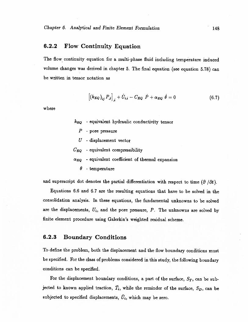
Chapter 6. Analytical and Finite Element Formulation 148
6.2.2 Flow Continuity Equation
The flow continuity equation for a multi-phase fluid including temperature induced
volume changes was derived in chapter 5. The final equation (see equation 5.78) can
be written in tensor notation as
[(kEQ)F] —1 +czEQ = 0 (6.7)
where
kEQ - equivalent hydraulic conductivity tensor
P - pore pressure
U - displacement vector
CEQ - equivalent compressibility
aEQ - equivalent coefficient of thermal expansion
6 - temperature
and superscript dot denotes the partial differentiation with respect to time (8 /8t).
Equations 6.6 and 6.7 are the resulting equations that have to be solved in the
consolidation analysis. In these equations, the fundamental unknowns to be solved
are the displacements, U, and the pore pressure, P. The unknowns are solved by
finite element procedure using Galerkin’s weighted residual scheme.
6.2.3 Boundary Conditions
To define the problem, both the displacement and the flow boundary conditions must
be specified. For the class of problems considered in this study, the following boundary
conditions can be specified.
For the displacement boundary conditions, a part of the surface, can be sub
jected to known applied traction, while the reminder of the surface, SD, can be
subjected to specified displacements, U, which may be zero.

Chapter 6. Analytical and Finite Element Formulation 149
For the flow boundary conditions, it is assumed that part of the boundary surface,
Sp, is subjected to specified pore pressures, F, which can be set to zero to simulate
a free draining surface. The reminder of the surface, 5q is considered impermeable,
i.e. there is no flow across the boundary.
Mathematically, these boundary conditions can be expressed as
a1n3=t for t0 (6.8)
U = (J for t 0 (6.9)
P=P for t>0 (6.10)
for t0 (6.11)
where n is the normal vector to the boundary surface and the bar symbol indicates
a prescribed quantity.
To complete the description of the problem, the initial conditions must also be
defined. At t = 0, since there is no time for the fluid to be expelled, the volume
change in the pore fluid and in the soil skeleton must be equal. Thus,
tSv = CEQ P at t = 0 (612)
6.3 Drained and Undrained Analyses
The drained and undrained analyses can be easily performed by considering only
the equilibrium equation (equation 6.6). The flow continuity equation need not be
considered under drained and undrained conditions. The drained analysis is quite
straight forward as it just involves solving the equilibrium equation. However, to
perform an undrained analysis some modifications have to be made.
Generally, the undrained response is analyzed with total stress parameters and
the analytical formulation has to be in terms of total stresses. If the pore pressures
are desired, they are commonly computed from the Skempton equation relating total

Chapter 6. Analytical and Finite Element Formulation 150
stress changes to pore pressure parameters. To use the effective stress formulation for
undrained analysis, Byrne and Vaziri (1986) adopted an approach similar to the one
proposed by Naylor (1973). In this approach, the stiffness matrix for a total stress
analysis is obtained from the effective stress parameters and from the compressibility
of the fluid components as described in this section. The solution procedure is then
carried out in the usual manner for a total stress analysis to obtain deformations. The
pore pressures can be evaluated from the computed deformations using the relative
contributions of the pore fluid and the skeleton, without the use of the Skempton
equation.
The incremental effective stresses are related to the incremental strains by the
following relationship:
{o’} = [D’] {L} (6.13)
where
{ e} - strain vector
{ o’} - effective stress vector
[D’] - matrix relating effective stress and strain
The volumetric strain can be expressed as
= {m}T{e} (6.14)
where {m}T = {1 1 1 0 0 0} , is a vector selected such that only direct strains will
be involved in the volumetric strain.
For undrained conditions, the volume compatibility requires that the volume
change in the skeleton equals the volume change in the fluid, i.e.,
= (6.15)
where
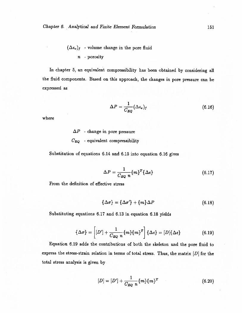
Chapter 6. Analytical and Finite Element Formulation 151
(Lc)j - volume change in the pore fluid
n - porosity
In chapter 5, an equivalent compressibility has been obtained by considering all
the fluid components. Based on this approach, the changes in pore pressure can be
expressed as
(6.16)
where
- change in pore pressure
CEQ - equivalent compressibility
Substitution of equations 6.14 and 6.15 into equation 6.16 gives
= 1{m}T{E} (6.17)
CEQ
From the definition of effective stress
{o-} = {&r’} + {m}i.P (6.18)
Substituting equations 6.17 and 6.13 in equation 6.18 yields
= [[D’l +1
{m}{m}T] {e} = [D]{e} (6.19)CEQ ‘
Equation 6.19 adds the contributions of both the skeleton and the pore fluid to
express the stress-strain relation in terms of total stress. Thus, the matrix [D] for the
total stress analysis is given by
[D] = [D’] +1
{m}{m}T (6.20)CEQ

Chapter 6. Analytical and Finite Element Formulation 152
Equation 6.19 is used in the finite element formulation for undrained conditions.
The pore pressure is not an unknown in the resulting system of equations, but is
obtained from equation 6.17, once the deformations are computed.
Byrne and Vaziri (1986) claimed that this method has definite advantages such
as adaptability for saturated or unsaturated soils and for any stress-strain relation.
In particular, this method gives stable solutions when the effective stresses go to zero
and all of the load is carried by the pore fluid. For an incompressible fluid, CEQ
becomes zero and the above formulation becomes ill-conditioned. However, this can
be overcome by setting the value of CEQ to a suitably low but finite value (Naylor,
1973).
6.4 Finite Element Formulation
The equations governing the consolidation with multi-phase fluid and temperature
effects have been derived and are given by equations 6.6 and 6.7. The best method of
obtaining a solution for these equations is to use a numerical technique such as finite
element method. The finite element procedure can be formulated in a number of ways.
For instance, Sandhu and Wilson (1969) used a Gurtin type variational principle.
Booker and Small (1975) employed a variational theorem involving Laplace trans
formations. Christian and Boehmer (1970), Carter (1977) and Small et al. (1976)
obtained the solutions through the principle of virtual work. Hwang et al. (1972)
and Chang and Duncan (1983) used the weighted residual technique to develop the
finite element formulation.
The choice of the different approaches depends on the type of the problem and the
boundary conditions on one hand, and the knowledge of the mathematics involved
on the other hand. In this study, Galerkin’s weighted residual scheme is used to
develop the finite element formulations. The weighted residual scheme is quite straight
forward, has relatively less mathematics involved, and is less error prone. In the

Chapter 6. Analytical and Finite Element Formulation 153
Galerkin scheme only a single application of Green’s theorem is needed to obtain a
set of integral equations. These equations can be easily turned into matrix form and
solved. However, it should be noted that regardless of the approach used, whether
weighted residual or variational principle, the end results will be the same.
From the previous section, the governing differential equations to be solved are,
(Uk,j + UZk)j + + — 0 (6.21)
[(kEQ) + — CEQ F + aEQ = 0 (6.22)
To develop the finite element formulation for these equations, the domain being
analyzed is subdivided into a finite number of elements. The quantities of the four
independent variables within each of the elements, U and F, are approximately repre
sented by means of shape functions and their values at the nodes. The equations 6.21
and 6.22 have at most second order derivatives of displacements and pore pressures.
However, by applying Green’s theorem, it can be reduced to first order. Therefore, to
solve the resulting integral equations the shape functions for displacements and the
pore pressure should be continuous. Hence, the displacement and the pore pressure
fields within the element can be written as
U = N e (6.23)
(6.24)
where
5eT= {S, S2, . . , S} (nodal displacements)
q = {qi, q,.. . , q} (nodal pore pressures)
U’ - displacement field
- pore pressure field

Chapter 6. Analytical and Finite Element Formulation 154
N - shape functions for displacements
- shape functions for pore pressures
U” and F” are approximate solutions and substituting these values into equations
6.21 and 6.22 will not exactly satisfy the equations, but will give some residual errors
as follow:
[Dkl ± + z1 + [D — (6.25)
[(kEQ F], + U”,1 — CEQ F” + aEQ S (6.26)
In the weighted residual scheme, these residual errors are minimized in some
fashion to give the best approximate solution. Thus, for the best solution
jwrdv=O (6.27)
where
r - residual error
w - weighting function
In Galerkin’s scheme the weighting functions are chosen to be the same as the
assumed shape functions. Then the following equations can be obtained to minimize
the residual errors r1 and r2:
j Nr1dv = 0 (6.28)
jNpr2dvzO (6.29)
The strains and the derivative of the pore pressure within an element can be
written as

Chapter 6. Analytical and Finite Element Formulation 155
(6.30)
= m’ (6.31)
B Iq6 (6.32)
where
mT ={1 1 100 0}
B & B - shape function derivatives
Green’s theorem for integration involving two functions, and over the domain
can be expressed as
J ç V dIZ= j c (V) dF
— j V V d1 (6.33)
where, I’ is the boundary around and i is the normal to the boundary.
By substituting equations 6.23 to 6.26 and 6.30 to 6.32 into equations 6.28 and
6.29, and by applying Green’s theorem, one obtains
j BDB,4Sdv + / B’mNqdv = / NTds + j NFdv - / B’Dedv
(6.34)
— / BkEq Bqdv H- / NpTmTBuSdv — / CEQN1’Ndv = — / NpTaeq6dv (6.35)
For a time increment t the above set of equations can be written in matrix form
as
[K] {i6} + [L] {q} = {A} (6.36)

Chapter 6. Analytical and Finite Element Formulation 156
[L]T {S} - t [E] {q} - [G] {q} = -{C} (6.37)
where
[K] =fBDBdv
[U =fBmNdv
rr1l p DTI r,L-’J — Jv -0p nEQ L’p
[G] =fCEQNNpdv
{LA} = f8 NTds + f NFdv— f B,D6ed
{zXC} fvNp0eqMdt
Equation 6.37 is considered over a time increment t, and therefore, the term q
in that equation has to be expressed as,
q = (1—
a)qt + aqt (6.38)
where a is a parameter corresponding to some integration rule. For example, a = 1/2
implies trapezoidal rule, a = 0 implies a fully explicit method and a = 1 gives a fully
implicit method. Booker (1974) showed that for an unconditionally stable numerical
integration a 1. In the formulation here, the value of a is assumed to be 1,
i.e. a fully implicit method. Thus, the term q in equation 6.37 can be given as,
q = qt+t = qt + q (6.39)
Substitution of equation 6.39 into equation 6.37 yields,
[U]T {8} — t [E] {qt + Lq} — [C] {q} = —{zC} (6.40)
By rearranging the terms,
[U]T {zS} — zSt [[E] — [G]] {q} = —{zC} + [E]qtt (6.41)
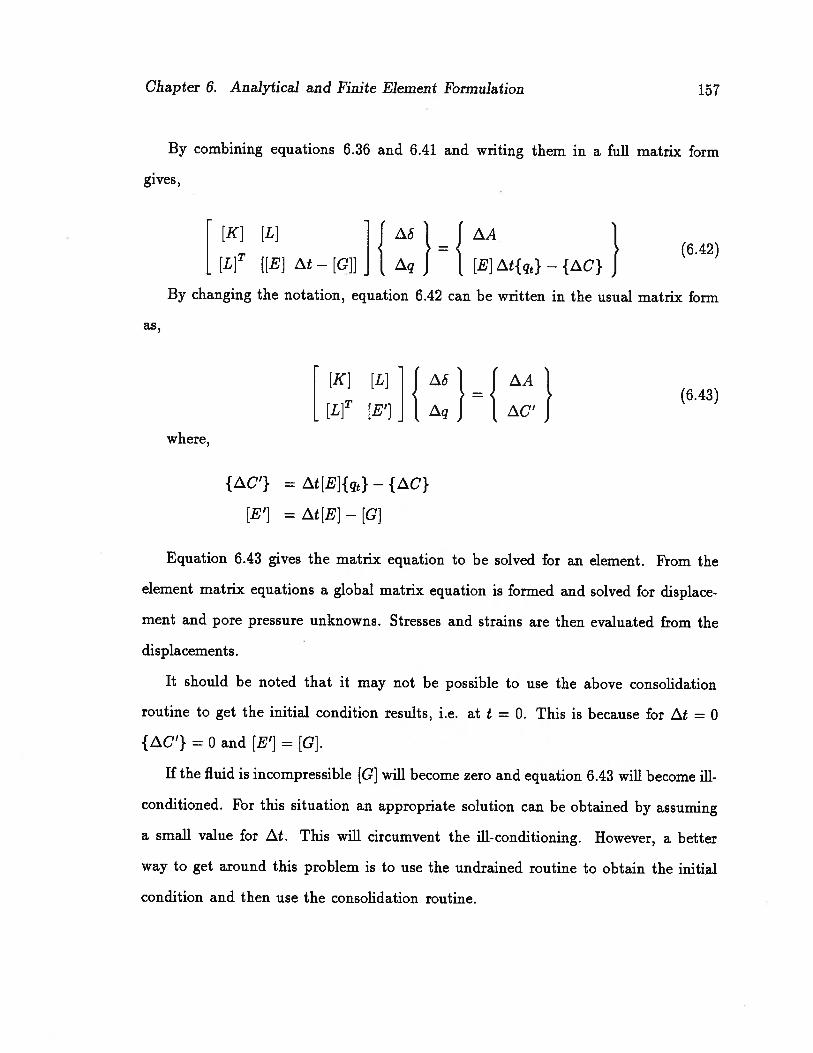
Chapter 6. Analytical and Finite Element Formulation 157
By combining equations 6.36 and 6.41 and writing them in a full matrix form
gives,
[K] [L] z8 1A ‘1(6.42)
[L]T [[E] Lt — [G]] Lq J [E] /.t{qt} — {tC} JBy changing the notation, equation 6.42 can be written in the usual matrix form
as,
[K] [L] ILS1 1A1(6.43)
[L]T [E’] q J LC’ Jwhere,
{LW’} = tt[E}{qt} - {C}
[E’] =t[E]-[G]
Equation 6.43 gives the matrix equation to be solved for an element. From the
element matrix equations a global matrix equation is formed and solved for displace
ment and pore pressure unknowns. Stresses and strains are then evaluated from the
displacements.
It should be noted that it may not be possible to use the above consolidation
routine to get the initial condition results, i.e. at t = 0. This is because for Lt = 0
{zC’} = 0 and [E’] = [G].
If the fluid is incompressible [G] will become zero and equation 6.43 will become ill
conditioned. For this situation an appropriate solution can be obtained by assuming
a small value for t. This will circumvent the ill-conditioning. However, a better
way to get around this problem is to use the undrained routine to obtain the initial
condition and then use the consolidation routine.
Chapter 6. Analytical and Finite Element Formulation 158
6.5 Finite Elements and the Procedure Adopted
The principal steps and the details such as obtaining shape functions, its derivatives,
formulation of stiffness matrix, numerical integration, etc., can be found in any stan
dard finite element text book. Therefore, only a summary with some discussions on
certain issues which are important for the class of problems considered in this study,
are given in this section. The developed analytical model has been incorporated in
an existing 2-dimensional finite element code, CONOIL-Il (Srithar (1989)) and also
in a new 3-dimensional finite element code, CONOIL-Ill. The following subsections
address the key aspects in the development of these finite element codes.
6.5.1 Selection of Elements
The choice of the finite elements has been an important issue when analyzing con
solidation problems. Different researchers used different element types. Sandhu and
Wilson (1969) introduced a composite element, consisting of a six-noded triangle for
the displacements expansion, and only three nodes being used for the pore pressure ex
pansion. The displacements varied quadratically over the element, while the stresses
and strains obtained by differentiating the displacements varied linearly. Since the
pore pressures are expressed in terms of three nodal values, they vary linearly too.
Therefore, the element has the same order of expansion for both stress components
and pore pressures. Yooko et al. (1971a) used several different elements, all of which
used the same expansion for the displacements and for the pore pressures. This makes
N = N for any choice of element and the relevant matrices can be derived easily.
The examples they presented include a two noded bar element, a three noded ax
isymmetric triangular ring element an a four noded rectangle. However, Yooko et
al. (1971b) had difficulties in obtaining reasonable results for the initial undrained
conditions. Sandhu et al. (1977) also compared several finite elements and concluded
Chapter 6. Analytical and Finite Element Formulation 159
that the elements which had the same expansion for displacement and pore pressures
do not give satisfactory answers at the initial stages of consolidation. However, they
claimed that at later stages of consolidation, the differences in the results for different
element types are insignificant.
Ghaboussi and Wilson (1973) used an isoparametric element of four nodes with
the standard expansion for pore pressures and two additional nonconforming degrees
of freedom for the displacement expansion. The two additional degrees of freedom are
eliminated by static condensation after the element stiffness is completed. However,
this procedure does not give the same expansion for pore pressures and stresses, but
uses a lower order expansion for pore pressures than for displacement.
In the 2-dimensional finite element code employed in this study, element types sim
ilar to those proposed by Sandhu and Wilson (1969) are used. Figure 6.1 shows the
two different triangular elements used for consolidation analysis in the 2-dimensional
code. Figure 6.2 shows the element types available in the 3-dimensional code. The
eight-noded brick element uses the same expansions for pore pressures and displace
ments, whereas the 20-noded brick element uses different shape functions for displace
ments and pore pressures.
6.5.2 Nonlinear Analysis
The solution of the nonlinear problems by the finite element method is usually
achieved by one of the following techniques:
1. Incremental or stepwise procedures
2. Iterative or Newton method
3. Step-iterative or mixed procedures
The method employed herein is a form of the mixed procedure which follows
the midpoint Runge-Kutta or modified Euler method. In this scheme, two cycles
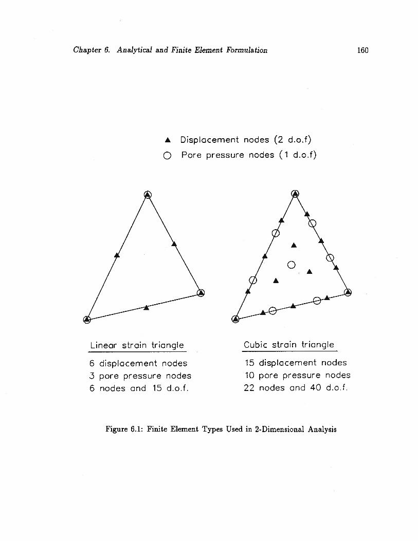
Chapter 6. Analytical and Finite Element Formulation 160
A Displacement nodes (2 d.o.f)
Q Pore pressure nodes (1 d.o.f)
Linear strain triangle
6 displacement nodes
3 pore pressure nodes
6 nodes and 15 d.o.f.
Cubic strain triangle
15 displacement nodes
10 pore pressure nodes
22 nodes and 40 d.o.f.
Figure 6,1: Finite Element Types Used in 2-Dimensional Analysis
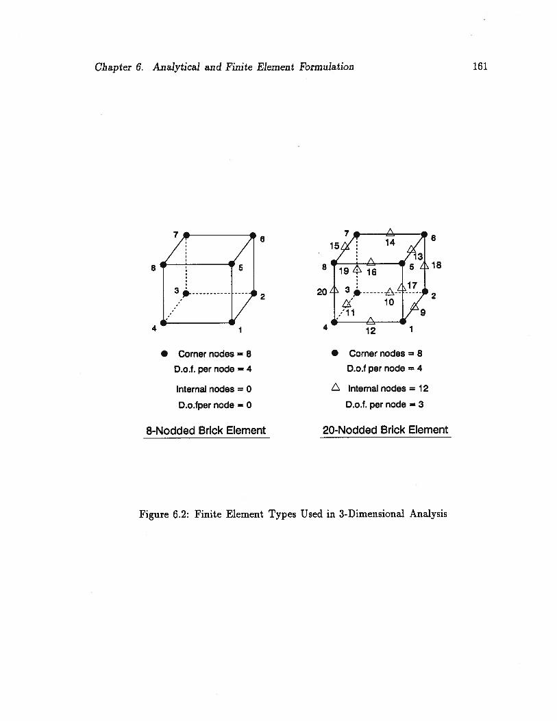
Chapter 6. Analytical and Finite Element Formulation
5I
161
• Corner nodes = 8
D.o.f. per node = 4
Internal nodes = 0
D.o.fper node = 0
8-Nodded Brick Element
• Corner nodes = 8
D.o.f per node = 4
A Internal nodes = 12
D.o.f. per node = 3
20-Nodded Brick Element
8
A
157
,.
14
A
6
188
20
44 1
19Li16
s34 A-4-10
/11A
12
Figure 6.2: Finite Element Types Used in 3-Dimensional Analysis

Chapter 6. Analytical and Finite Element Formulation 162
of analysis are performed for each load increment. In the first cycle of analysis,
parameters based on the initial .conditions of the increment are used.. At the end of
first cycle, parameters at the midpoint of the load increment are computed. In the
second cycle, the midpoint parameters are used to analyze the load increment and the
final results are evaluated. To obtain more accurate results, this process would have
to be continued until the difference between successive results satisfies the specified
tolerance. Such an iterative procedure can increase the computer time drastically
and therefore, was not employed. However, an improvement in the results is made
by estimating the imbalance load at the end of second cycle and adding that to the
next load increment.
6.5.3 Solution Scheme
Selection of the method for solving the simultaneous algebraic equations is a major
factor influencing the efficiency of any finite element program, and there are variety of
solution techniques to choose from. Essentially, there are two classes of methods; one
is the direct solution methods and the other is the iterative solution methods. The
direct methods use a number of exactly predetermined steps and operations, whereas
the iterative methods make an approximation to solve the equations.
The most effective direct solution methods are basically variations of the Gaussian
elimination method. Most of the methods take advantage of specific properties of the
stiffness matrix, its symmetry, its positive definiteness or its banded nature to reduce
the number of operations and the storage requirements to accomplish a solution.
Bathe and Wilson (1970) and Meyer (1973) discussed the relative merits of the current
popular methods, and both of these references contain extensive bibliography.
The frontal solution scheme for symmetric matrices (Irons, 1970) and for unsym
metric matrices (Hood, 1976) have been employed in the finite element codes. In the
frontal solution scheme, the element stiffness matrices are assembled and solved by
Chapter 6. Analytical and Finite Element Formulation 163
Gaussian elimination and back substitution process, but the overall global stiffness
matrix is never formed. The variables are introduced at a later stage and eliminated
earlier than in most of the other direct solution methods. Since the variables are
eliminated as soon as conceivably possible, the operations with zero coefficients are
minimized and the total arithmetic operations are fewer. As a result, it is faster and
requires less core memory than band routines. In addition, it is not necessary to
apply a stringent node numbering scheme. Its efficiency is essentially a function of
element numbering.
Theoretically, the frontal solution scheme will always perform better or at least
as well as the bandwidth solving routines in terms of accuracy and efficiency (Irons,
1970; Irons and Ahmad, 1980). Some comparisons have already given in the literature
to substantiate this claim (eg: Sloan 1981; Light and Luxmore, 1977; Hood, 1976).
The frontal solution scheme is specially attractive for unsymmetric matrices because
less computer storage is required. The stress-strain model considered in this study
deals with a nonassociated flow rule which results in an unsymmetric stiffness matrix
and therefore, using the frontal solution scheme has a definite advantage.
The main disadvantage of this method is the complexity of the internal book
keeping. However, the bookkeeping is a programming problem and does not concern
the user. Another limitation of this technique may be its dependence on the element
numbering sequence. Although it is rather easier to number the elements in a logical
manner relative to numbering the nodal sequence, it does place some effort on the
user. However, the difficulty can be easily dealt with, if some form of front width
minimizer is incorporated in the program. There are different front width minimizing
schemes available such as by Sloan and Randolph (1981), Akin and Pardue (1975)
and Pina (1981). The procedure by Sloan and Randolph (1981) is built into the
2-dimensional finite element code.
Chapter 6. Analytical and Finite Element Formulation 164
6.5.4 Finite Element Procedure
A broad overview of the procedures followed in both, the 2-dimensional and 3-
dimensional programs is given in the flow chart shown in figure 6.3. The steps involved
in the finite element procedure can be summarized as follows:
1. Basic data such as the number of nodes, elements and material types are read
and the required storage is allocated for the variables.
2. All other data such as nodal coordinates, temperatures, element-nodal informa
tion and model parameters are read.
3. The initial conditions are read and the initial stresses, strains, pore pressures
and force vectors are set.
4. Relevant data for the load increment is read.
5. Force vector and the element stiffness matrices are evaluated using the moduli
based on the initial stresses.
6. The equations are solved using the frontal solution scheme. For linear and
nonlinear elastic stress-strain models, the solution scheme for symmetric matri
ces is used. For the elasto-plastic stress-strain model, the solution scheme for
unsymmetric matrices is used.
7. Increments in the stresses and strains for the load increment are calculated and
if it is the first cycle of analysis, new moduli are evaluated based on the stresses
at the mid point of the increment.
8. If it is the first cycle of analysis, steps 5 to 7 are repeated once more using new
moduli for step 5.
9. The stresses, strains and pore pressures and other relevant results are calculated
and the desired results are printed.

Chapter 6. Analytical and Finite Element Formulation 165
C Start DRead basic data and allocate storage
for principal arrays
Read and set the initial conditions
Read relevant data for theload increment
Evaluate stiffness matrix and load vector
Solve for displacements and pore pressures
Evaluate the changes in stresses,strains and pore pressures
Update relevantIs this the last cycle No
variables toof analysis’ average values
Yes
riJpdate all the results and print
No
NoLast increment?
Yes
C Stop D
Figure 6.3: Flow Chart for the Finite Element Programs

Chapter 6. Analytical and Finite Element Formulation 166
10. If the current stress state exceeds the strength envelope, or if there is strain
softening, load shedding vector is computed.
11. Steps 5 to 9 are repeated until all the elements satisfy the failure criterion or in
other words, until the load shedding is converged.
12. The imbalance loads at the end of the increment are calculated and added to
the next load increment, if any.
13. Steps 4 to 12 are repeated until all the load increment data have been analyzed.
The final states of the previous load increment are used as the initial conditions
for the next load increment.
6.6 Finite Element Programs
The finite element programs have been written in FORTRAN-77 and are portable
to any operating platforms. There are two separate programs; CONOIL-Il which
is a 2-dimensional program to perform axisymmetric and plane strain analyses and,
CONOIL-Ill which is a 3-dimensional program to perform 3-dimensional analysis. Al
though these finite element programs have been developed with special attention paid
to the problems in oil sand, they are capable of doing general drained, undrained and
consolidation analyses effectively. Both programs are capable of analyzing excavations
as well. Brief descriptions of these programs are given in this section. Applications
of the programs are discussed later in chapter 7.
6.6.1 2-Dimensional Program CONOIL-Il
The 2-dimensional program CONOIL-Il was originally developed by Vaziri (1986)
based on the program CRISP (University of Cambridge). It was later modified by

Chapter 6. Analytical and Finite Element Formulation 167
Srithar in 1989 with an improved formulation for temperature analysis. CONOIL
II has been divided into two separate programs; the ‘Geometry Program’ and the
‘Main Program’. The main purpose of this split is to reduce the effort for the user.
The geometry program automatically generates and numbers the midside and interior
nodes. It also renumbers the elements and nodes to minimize the front width and
creates a input file for the main program, containing the relevant information about
the finite element mesh. The program also has some special features. The triple
matrix product as suggested by Taylor (1977) is adopted in the formation of stiffness
matrix, and this will eliminate all the unnecessary arithmetic operations which will
result in zero coefficients. The geometry program consists of 11 subroutines and the
main program consists of 58 subroutines. The names of the subroutines and their
functions are presented in appendix C.
Grieg et al. (1991) developed a pre/post processor package, COPP, for CONOIL
II to facilitate viewing and plotting the CONOIL-Il input and output data. COPP
is menu driven, very user friendly and provides many options for the user.
6.7 3-Dimensional Program CONOIL-Ill
The 3-dimensional program CONOIL-Ill has been developed from scratch following
the same sequence of procedures as the 2-dimensional one. However, compared to
the 2-dimensional program, the 3-dimensional program has less special features, and
it does not have a post processor yet. The 3-dimensional program comprises 43
subroutines. The names of the subroutines and their functions are given in appendix
C. A User manual and some example problems are presented in appendix F.
Chapter 7
Verification and Application of the Analytical
Procedure
7.1 Introduction
The analytical procedure described in chapter 6 has been incorporated in the finite
element program, CONOIL. The main intention of this chapter is to verify and val
idate the finite element program, and to demonstrate its applicability. The program
deals with a number of aspects such as, dilative nature of sand, three-phase pore fluid,
gas exsolution, effects of temperature changes, etc.. and the best way of verifying the
program would be to consider each aspect separately. The program is verified here
by considering some particular problems for which theoretical solutions are available.
Once verified, the program is validated by comparing some experimental results with
predictions from the program. Then, the program has been used to predict the re
sponses in a oil recovery problem. A problem concerning pore pressure redistribution
after liquefaction has also been analyzed to show the applicability of the program to
other geotechnical problems.
7.2 Aspects Checked by Previous Researchers
The two dimensional version of the finite element program CONOIL has been used at
the University of British Columbia since 1985, with improvements being made from
time to time. Cheung (1985), Vaziri (1986) and Srithar (1989) have demonstrated
the capability of the program on a number of aspects. Since those aspects are kept
168
Chapter 7. Verification and Application of the Analytical Procedure 169
intact with the improvements made in this study, those verifications and validations
are still valid. These are briefly described herein.
The general performance of the program in predicting stresses and strains has
been verified by Cheung (1985), by considering a thick wall cylinder under plane
strain conditions. Closed form solutions for this problem have been obtained from
Timoshenko (1941). The results from the program and the closed form solutions are
in excellent agreement and are shown in figure 7.1.
Cheung (1985) also validated the gas exsolution phenomenon in the program.
Laboratory test results by Sobkowicz (1982) on gassy soil samples have been consid
ered. Sobkowicz (1982) carried out triaxial tests to predict the short term undrained
response, i.e, no gas exsolution and the long term undrained response, i.e., with com
plete gas exsolution, The comparisons of the test results with the program results are
shown in figures 7.2 and 7.3. The measured and predicted results agree very well.
The overall structure of operations for a consolidation analysis has been verified
by Vaziri (1986). The closed form solution developed by Gibson et al. (1976) for
a circular footing resting on a layer of fully saturated, elastic material with finite
thickness has been considered for the verification. A comparison of the computed
results and the closed form solutions, shown in figure 7.4, demonstrate that they are
in very good agreement.
Srithar (1989) modified the procedure for thermal analysis in the original CONOIL
formulation. He verified the new formulation under drained and transient conditions.
The closed form solution presented by Timoshenko and Goodier (1951) for a long
elastic cylinder subjected to temperature changes has been considered to verify the
formulation under drained condition. The closed from solution and the finite element
results are shown in figure 7.5 and are in remarkably good agreement.
To verify the formulation for thermal analysis under transient conditions, a closed
form solution was derived by Srithar (1989) for one dimensional thermal consolidation
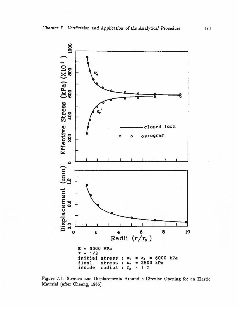
Chapter 7. Verification and Application of the Analytical Procedure 170
0e0
0
0a)
closed form
o o 0programQca)
I I I I I I I I V
0
Ic’J
246810
Radii (r/r0)
E = 3000 MPaI’ — 1/3initial stress : or = o. = 6000 kPafinal stress : o = 2500 kPainside radius : r = 1 in
Figure 7.1: Stresses and Displacements Around a Circular Opening for an ElasticMaterial (after Cheung, 1985)

Chapter 7. Verification and Application of the Analytical Procedure 171
I.’
.-
C
b0
0
0C
Figure 7,2: Comparison1985)
of Observed and Predicted Pore Pressures (after Cheung,
00
40 60 80 100 120 140Total Stress (kPa) (X1O’ )
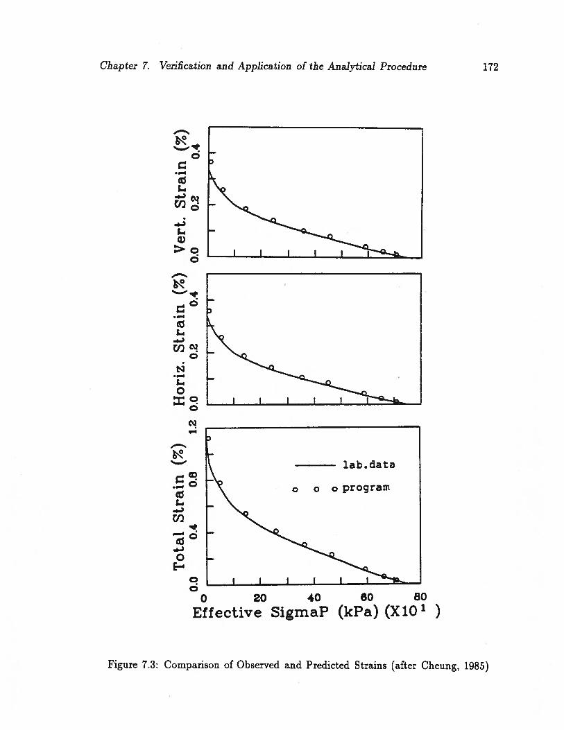
Chapter 7. Verification and Application of the Analytical Procedure 172
0
Cl2
.4.)
s-I
a)
>0
___________________
.—
s-I-I-)
0
s-I
0xc
____________________
0
lab data
0
l.a.4-’
Cl)
-4-’
0
0
___________________________
C0 20 40 60 80
Effective SigmaP (kPa) (X101 )
Figure 7.3: Comparison of Observed and Predicted Strains (after Cheung, 1985)

Chapter 7. Verification and Application of the Analytical Procedure 173
I I
0.25Analytical Solution
. Finite Element0.30 - Analysis
0.35-
________
r0.40 -
045 xI30y/30DIE—i .5
— 0.00.50
I I I I
ia-4 io io_2 1.0 10Ct
V
Tv-
a)Amount of settlement
0.0 I I I
Analytical Solution0.2-
‘%.‘b%,
0 Finite Element%, %\ Analysis
0.4
Uy/B—0 vO.3 v—0.0
0.6 — D/E — 1
0.8 -
1.0 I I
ia—4 i— 10—2 ia-’ 1.0 10Ct
V7 -—
U2
b) Degree of settlement
Figure 7.4: Results for a Circular Footing on a Finite Layer (after Vaziri, 1986)

Chapter 7. Verification and Application of the Analytical Procedure 174
3000 —
LaSymbols — CONOIL—IlSolid lines — Closed Form
2000 —
C
Vertical Stress1000—
Radial Stressci)
(1)
0—
Hoop Stress
—1000—
Radial Distance(m)
Figure 7.5: Stresses and Displacement in Circular Cylinder (after Srithar, 1989)
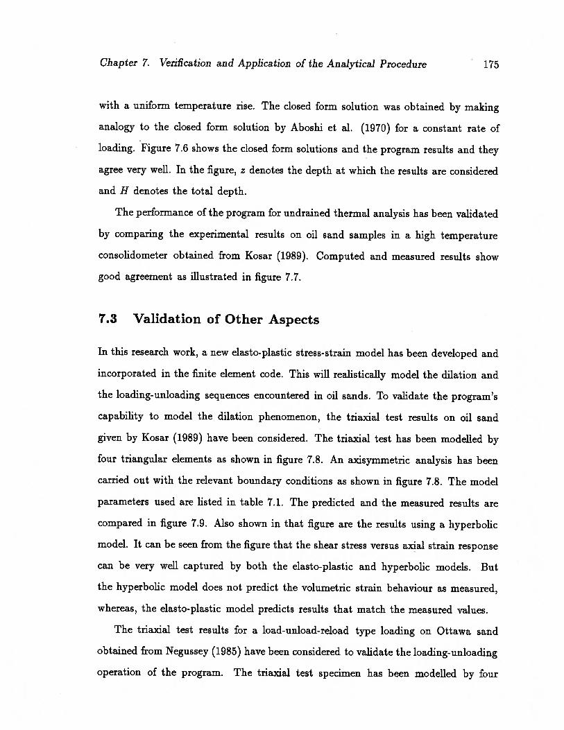
Chapter 7. Verification and Application of the Analytical Procedure 175
with a uniform temperature rise. The closed form solution was obtained by making
analogy to the closed form solution by Aboshi et al. (1970) for a constant rate of
loading. Figure 7.6 shows the closed form solutions and the program results and they
agree very well. [n the figure, z denotes the depth at which the results are considered
and H denotes the total depth.
The performance of the program for undrained thermal analysis has been validated
by comparing the experimental results on oil sand samples in a high temperature
consolidometer obtained from Kosar (1989). Computed and measured results show
good agreement as illustrated in figure 7.7.
7.3 Validation of Other Aspects
In this research work, a new elasto-plastic stress-strain model has been developed and
incorporated in the finite element code. This will realistically model the dilation and
the loading-unloading sequences encountered in oil sands. To validate the program’s
capability to model the dilation phenomenon, the triaxial test results on oil sand
given by Kosar (1989) have been considered. The triaxial test has been modelled by
four triangular elements as shown in figure 7.8. An axisymmetric analysis has been
carried out with the relevant boundary conditions as shown in figure 7.8. The model
parameters used are listed in table 7.1. The predicted and the measured results are
compared in figure 7.9. Also shown in that figure are the results using a hyperbolic
model. It can be seen from the figure that the shear stress versus axial strain response
can be very well captured by both the elasto-plastic and hyperbolic models. But
the hyperbolic model does not predict the volumetric strain behaviour as measured,
whereas, the elasto-plastic model predicts results that match the measured values.
The triaxial test results for a load-unload-reload type loading on Ottawa sand
obtained from Negussey (1985) have been considered to validate the loading-unloading
operation of the program. The triaxial test specimen has been modelled by four
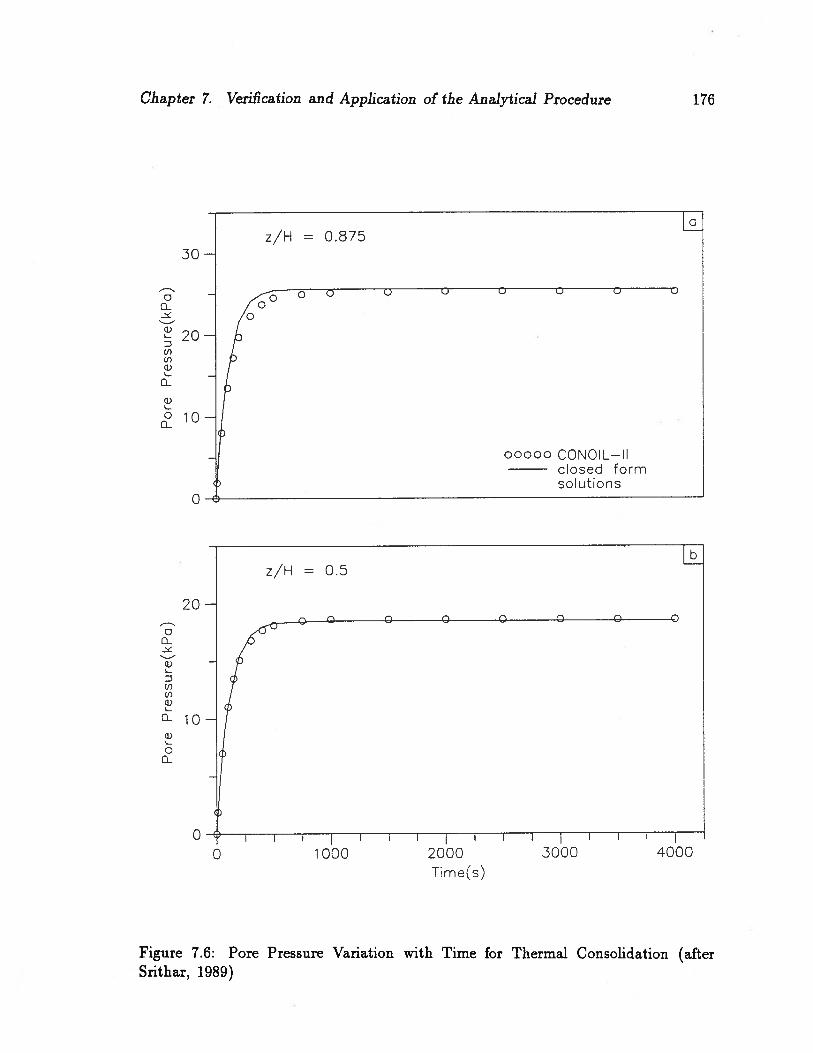
Chapter 7. Verification and Application of the Analytical Procedure 176
L’z/H = 0.875
30 —
0 0 0 0 ci p 0 0
0
- 2uCl)Cl,Q)
0
ci)
00000 CONOIL—Ilclosed formsolutions
0 —,
LHz/H = 0.5
20 —
C0
ci)
C
_
0 0
(1)
ci)
u-i0
00
0— i I I I I
0 1000 2000 3000 4000
Time(s)
Figure 7.6: Pore Pressure Variation with Time for Thermal Consolidation (afterSrithar, 1989)
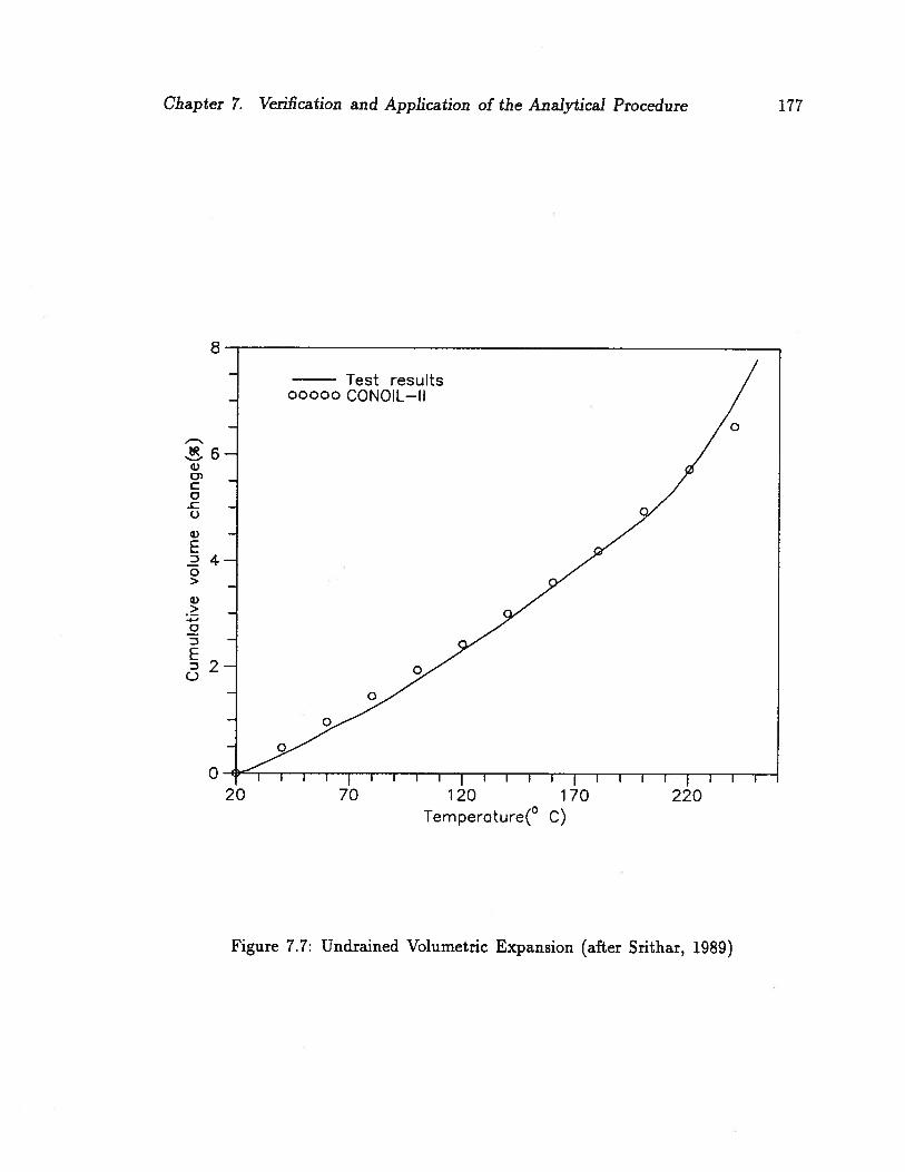
Chapter 7. Verification and Application of the Analytical Procedure 177
8-
Test results /00000 CONOIL—Il /
/0
6—a)
-
Cc-
- 0C-)
a) -
E2 4—0>
> -
D -
E0
0
0
0
I I I I I I I I I I
20 70 120 170 220Temperature(° C)
Figure 7.7: Undrained Volumetric Expansion (after Srithar, 1989)
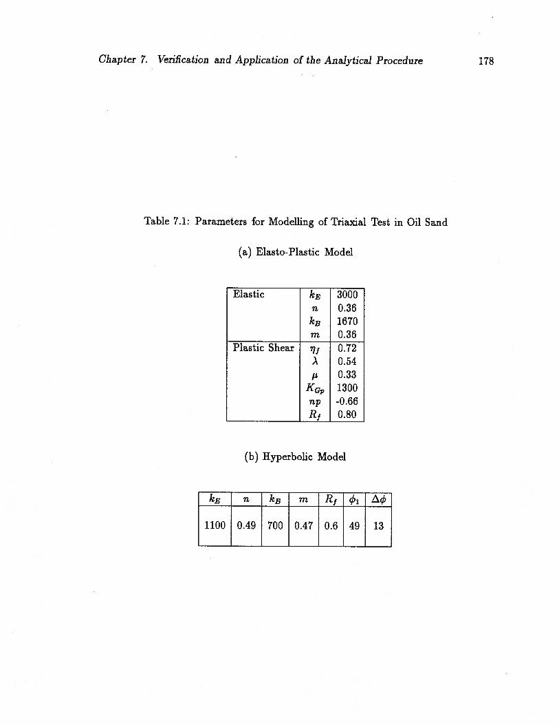
Chapter 7. Verification and Application of the Analytical Procedure 178
Table 7.1: Parameters for Modelling of Triaxial Test in Oil Sand
(a) Elasto-Plastic Model
Elastic kE 3000n 0.36
kB 1670m 0.36
Plastic Shear 0.72? 0.54
! 0.33KG 1300np -0.66Rf 0.80
(b) Hyperbolic Model
kE kB m R
1100 0.49 700 0.47 0.6 49 13

Chapter 7. Verification and Application of the Analytical Procedure 179
0
1.5 cm
Figure 7.8: Finite Element Modeffing of Triaxial Test
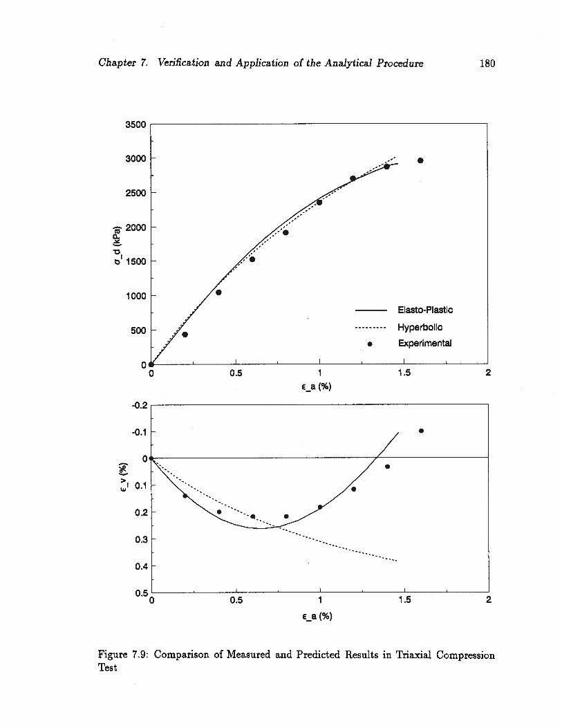
Chapter 7. Verification and Application of the Analytical Procedure
3500
3000
2500
‘a 20000S
‘0
1500
1000
500
‘I
WI
180
Figure 7.9: Comparison of Measured and Predicted Results in Triaxial CompressionTest
.
Elasto-Plastic
Hyperbolic
Experimental
Ea (%)
-0.2
-0.1
1
€_a (%)

Chapter 7. Verification and Application of the Analytical Procedure 181
elements as shown earlier in figure 7.8. The model parameters used are listed in table
7.2. The measured and predicted results agree very well as shown in figure 7.10.
Table 7.2: Model Parameters Used for Ottawa Sand
Elastic kE 3400m 0.0
kB 1888m 0.0
Plastic ‘i 0.49) 0.85IL 0.26
KG 780np -0.238R1 0.70
Modelling of the three-phase pore fluid is the other important aspect where major
improvements have been made in the analytical formulation in this study. There is
no theoretical or experimental solutions available to verify or to validate the overall
formulation for the modeffing of the three-phase pore fluid. However, validations for
the analytical representation of the relative permeabilities have been made and were
presented in chapter 5.
74 Verification of the 3-Dimensional Version
The 3-dimensional version of CONOIL is newly written following the same operational
framework as the 2-dimensional version. Since the 3-dimensional program is new, it
is necessary to check that the performance of the program in all aspects agrees with
the intended theories, as was proven for the 2-dimensional version. The problems
considered to verify the 3-dimensional code were similar to those used to verify the
2-dimensional code and all gave satisfactory results. Since the verifications are similar
to those presented in the previous sections, they are not repeated here. However, the
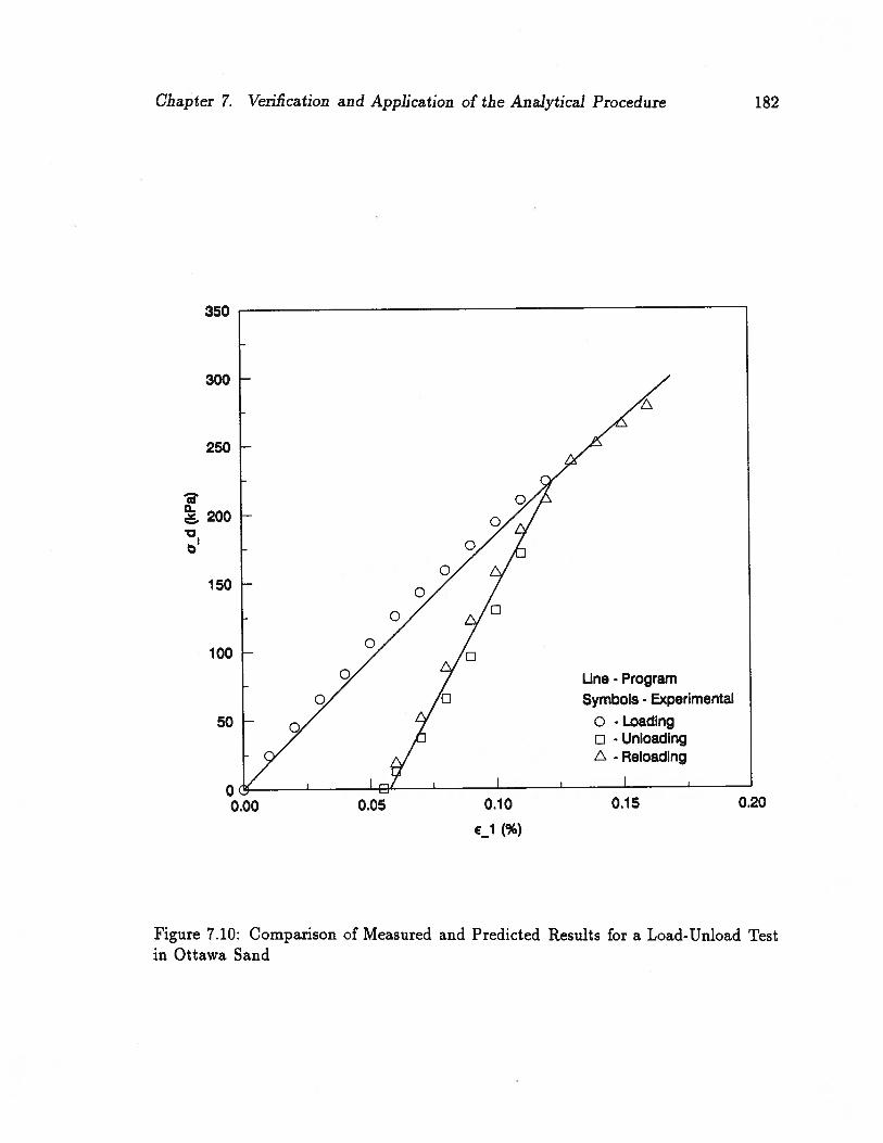
Chapter 7. Verification and Application of the Analytical Procedure 182
350
300
250
a. 200
150
100
50
0.00 0.20
Figure 7.10: Comparison of Measured and Predicted Results for a Load-Unload Testin Ottawa Sand
0.05 0.10 0.15
El (%)
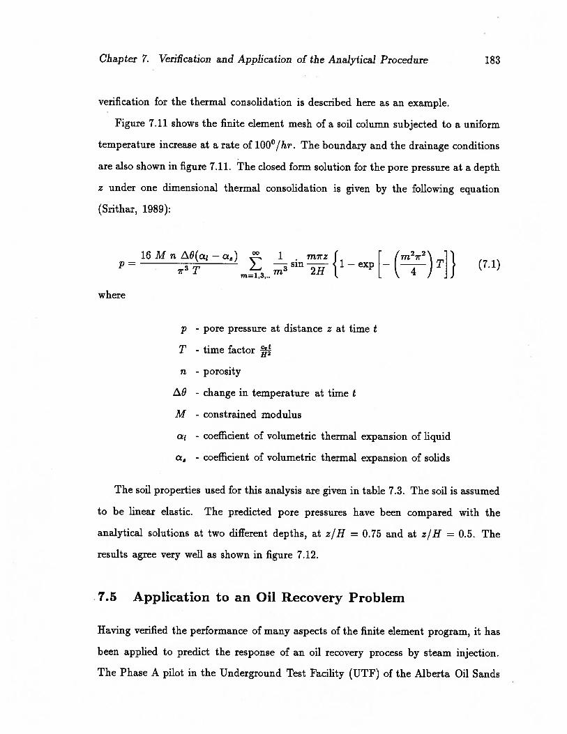
Chapter 7. Verification and Application of the Analytical Procedure 183
verification for the thermal consolidation is described here as an example.
Figure 7.11 shows the finite element mesh of a soil column subjected to a uniform
temperature increase at a rate of 100°/hr. The boundary and the drainage conditions
are also shown in figure 7.11. The closed form solution for the pore pressure at a depth
z under one dimensional thermal consolidation is given by the following equation
(Srithar, 1989):
16 M n — 1 mrz I (m2ir2’\ ‘1p r3 T m1,3,..
—i sin2H
— exp — T (7.1)
where
p - pore pressure at distance z at time t
T - time factor
n - porosity
- change in temperature at time t
M - constrained modulus
a1 - coefficient of volumetric thermal expansion of liquid
a8 - coefficient of volumetric thermal expansion of solids
The soil properties used for this analysis are given in table 7.3. The soil is assumed
to be linear elastic. The predicted pore pressures have been compared with the
analytical solutions at two different depths, at z/H = 0.75 and at z/H 0.5. The
results agree very well as shown in figure 7.12.
7.5 Application to an Oil Recovery Problem
Having verified the performance of many aspects of the finite element program, it has
been applied to predict the response of an oil recovery process by steam injection.
The Phase A pilot in the Underground Test Facility (UTF) of the Alberta Oil Sands
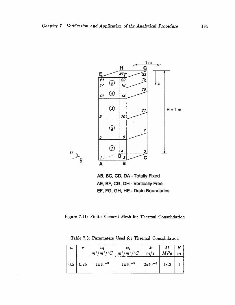
Chapter 7. Verification and Application of the Analytical Procedure 184
im
H G
__
21®22____3
13 ® 14
11 H=lm
_1O
7
5 6
z 4.. 3
.1
A B
AB, BC, CD, DA - Totally Fixed
AE, BF, CG, DH - Vertically Free
EF, FG, GH, HE - Drain Boundaries
Figure 7.11: Finite Element Mesh for Thermal Consolidation
Table 7.3: Parameters Used for Thermal Consolidation
fl V a1 a5 k M Hm3/m3/°C m3/m3/°C rn/s MPa rn
0.5 0.25 1x10³ 1x10⁵ 2x10⁶ 18.3 1

Chapter 7. Verification and Application of the Analytical Procedure 185
35z/H = 0.75
___________________________________________
(a)-
30
-25
20
01.
0I-.
00
10
Symbols - Program5 Line - Closed form
0 I I
0 500 1000 1500 2000 2500 3000 3500
Time (s)
30z/H = 0.5 (b)4Z
Symbols - ProgramLine - Closed form
0 I I I I I I
0 500 1000 1500 2000 2500 3000 3500
Time (s)
Figure 7.12: Comparison of Pore pressures for Thermal Consolidation

Chapter 7. Verification and Application of the Analytical Procedure 186
Technology and Research Authority (AOSTRA) is considered herein for analysis.
The UTF uses a steam assisted gravity drainage process with horizontal injection
and production wells. A brief description of the UTF and the problem to be analyzed
are presented here. Further details about the UTF can be found in Scott et al. (1992),
Laing et al. (1992) and in AOSTRA reports on UTF.
The UTF of AOSTRA is located near Fort McMurray, Alberta, and is currently
being used to test the shaft and tunnel access concept for bitumen recovery in deep
oil sand formations. The geological stratification at the UTF comprises a number of
soil layers. However, it can be simplified as consisting of three different soil types, in
a broad sense. Devonian Waterway formation limestone exists below a depth of 165
m. Overlying the limestone is the McMurray formation oil sand which is about 40 m
thick. The top 125 m overburden can be classified as Clearwater formation shale.
A schematic 3-dimensional view and a plan view of the UTF are shown in figures
7.13 and 7.14 respectively. There are two shafts accessing the tunnels in limestone
beneath the oil sand layer. The tunnels were constructed in the limestone at a depth
of about 178 m with the roof being about 15 m below the limestone-oil sand inter
face. Three pairs of horizontal injection and production wells were drilled from the
tunnels up into the oil sands at about 24 m spacing. A vertical section of the well
pairs was instrumented with thermocouples for measuring temperatures, pneumatic
and vibrating wire piezometers for measuring pore pressures and extensometers and
incinometers for measuring horizontal and vertical displacements.
Figure 7.15 shows a vertical cross-sectional view (section A-A’ in figure 7.14) of
the three well pairs. Modelling of all three well pairs with their steaming histories
and with the detailed geological stratification would be complex as the steaming
of different well pairs started at different times. To illustrate the problem and to
demonstrate the applicability of the program in a simple manner, only one well pair
is considered here for analysis.

Chapter 7. Verification and Application of the Analytical Procedure 187
Figure 7.13: A Schematic 3-Dimensional View of the UTF (after Scott et al., 1991

Chapter 7. Verification and Application of the Analytical Procedure 188
Shaft#1
I
TObservation Tunnel
i
Injector/Producer Wellpairs...... —
Section A-A’ —* Geotechnical A A’Cross Section
____ ____
4
Figure 7.14: Plan View of the UTF (after Scott et al., 1991)
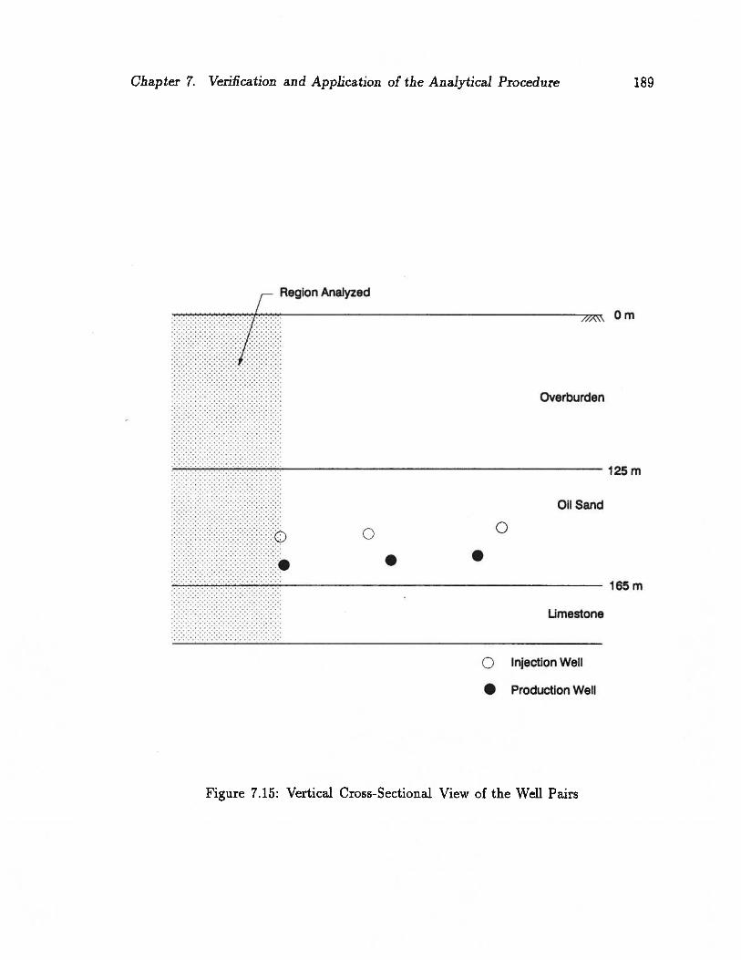
—.
....
..
......
......
..
..
V..:•:••
..
.•
.•.
..•.
.•.•
•.•
.•.•
.•.•.•.
.......
CD
CD -c
0C.
11
gg
0<
30
CD
CD=
U)
CD
CD0
=CD
CD0.
oC;
’C;
’3
33
00
Chapter 7. Verification and Application of the Analytical Procedure 190
To analyze the oil recovery with one well pair, the shaded region in figure 7.15 is
modelled by finite elements. The finite element mesh consisted of 240 linear strain
triangular elements as shown in figure 7.16. Plane strain boundary conditions are
assumed. The injection and production wells are modelled by nodes with known pore
pressures. The steam injection pressure is assumed to be maintained at 2800 kPa
(1300 kPa above the in-situ pore pressure) and the production pressure is assumed to
be at 2000 kPa (500 kPa above the in-situ pressure). The parameters used have been
obtained from laboratory test results reported by Kosar (1989) and from AOSTRA
and are listed in table 7.4. The gas saturation is assumed to be zero. i.e., the pore
fluid is assumed to comprise only water and bitumen. The bitumen saturation is
assumed to be 70 %.
The temperature-time histories of the nodes have also to be specified as an input
to the program. These were obtained from the field measurements made at the
UTF. The temperature contours in the oil sand layer at different times are shown in
figure 7.17. The steam chamber which is the region in the oil sand layer where the
temperature is the same the steam temperature, grows with time as shown in the
figure. At time t = 30 days, the steam chamber extends to a distance of about 10 m
horizontally and vertically from the injection well.
Even though a larger domain is analyzed as shown in the finite element mesh,
the results are plotted only for the oil sand layer which is of primary interest. The
predicted excess pore pressures in the oil sand layer are shown in figure 7.18. The
injection and production wells are also indicated in the figure. Figure 7.18 (a) shows
the excess pore pressure contours at 10 hours after the steam injection started. Only
a small region adjacent to the injection well experiences significant changes in the
pore pressures. This correlates very well with the temperature contours at that time,
as shown in figure 7.17 (a). With time, the region of higher pore pressure expands as
shown in figures 7.18 (b) and (c) indicating the growth of the steam chamber which
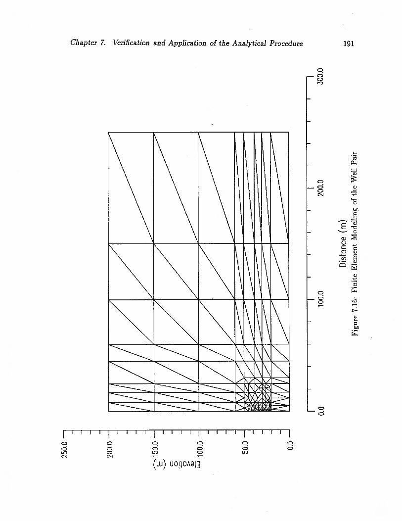
250.
0—
200.
0—
-150.0
Lii
100.
0—
50.0
—
0.0
—
22/7//
/////
22/?/
;c
0.0
1I
—I
I10
0.0
II
——
200.
0
II
II
300.
0
C-. 0
Dis
tanc
e(m
)F
igur
e7J
6:F
init
eE
lem
ent
Mod
ellin
gof
the
Wel
lP
air
I-.
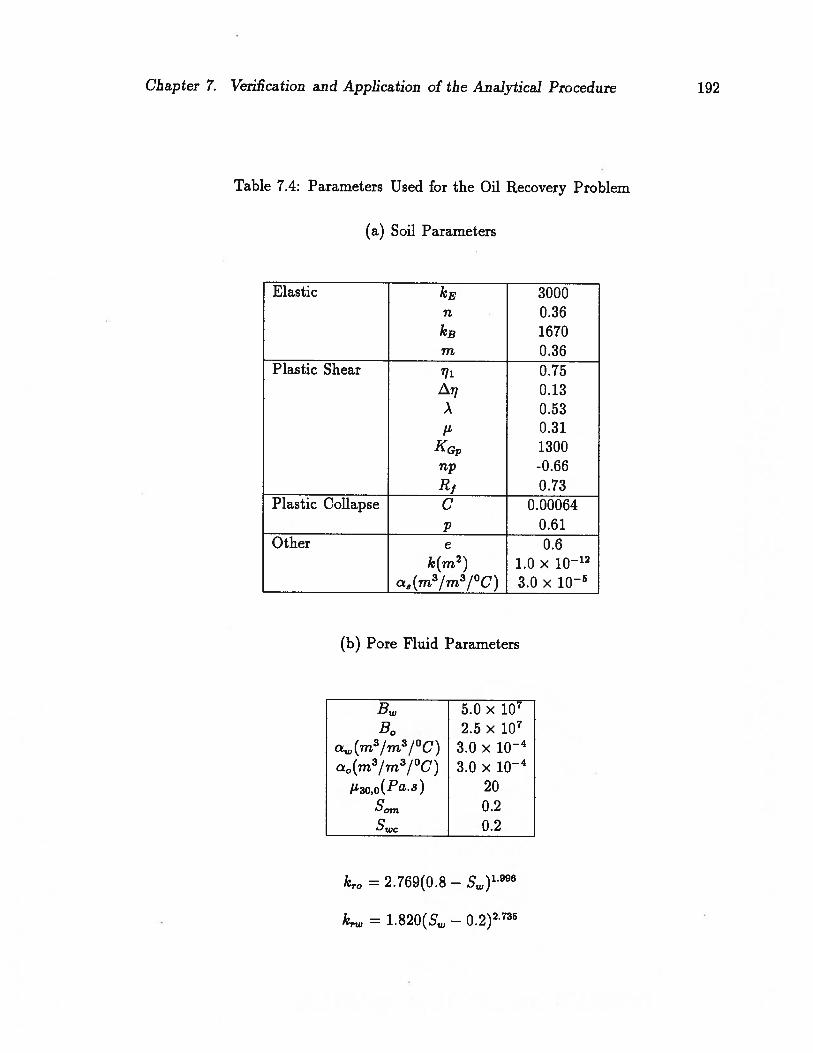
Chapter 7. Verification and Application of the Analytical Procedure 192
Table 7.4: Parameters Used for the Oil Recovery Problem
(a) Soil Parameters
Elastic 3000n 0.36
kB 1670m 0.36
Plastic Shear 171 0.75J.:l7 0.13). 0.53t 0.31
KG 1300rip -0.66R1 0.73
Plastic Collapse C 0.00064
p 0.61Other e 0.6
k(m2) 1.0 x 10—12
a8(m3/m3/°C) 3.0 x 1O
(b) Pore Fluid Parameters
B 5.0 x iOB0 2.5 x iO
cx(m3/m3/°C) 3.0 x i0cz0(m3/m3/°C) 3.0 x iO1u,o(Pa.s) 20
S 0.20.2
kro = 2.769(0.8 — S)’996
krw = 1.820(S — 0.2)2.735
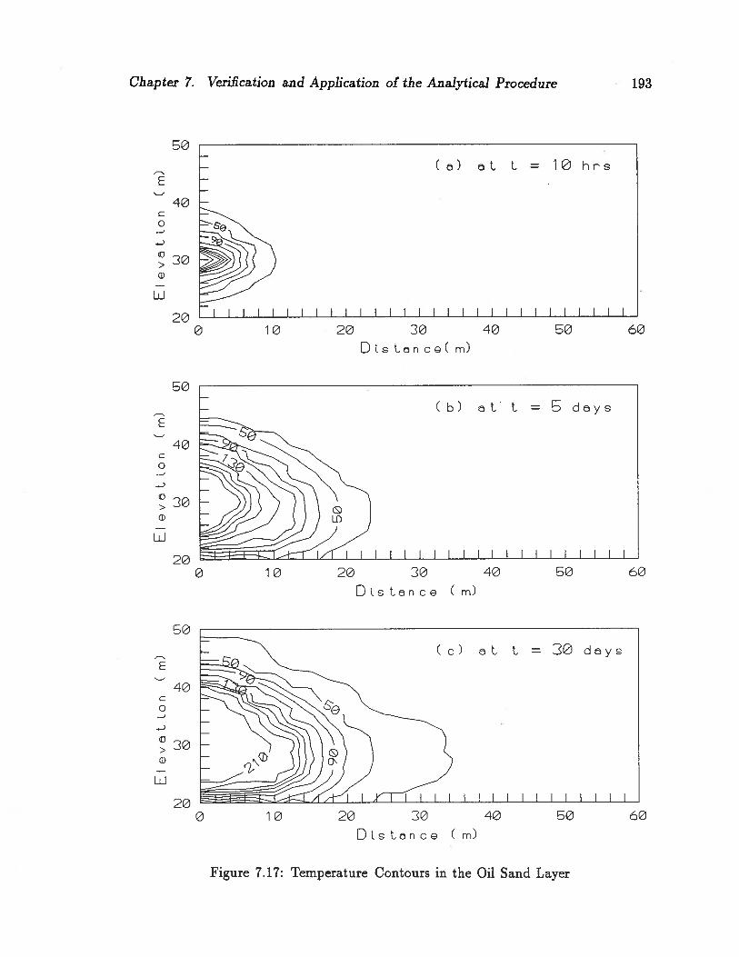
EIevL
on
(m)
EIev
Lo
n(m
)E
Iev
Lo
n(m
)
cyq CD CD p CD C)
0 0 cn CD 0 (j)
p CD
p I-’.
0
NJ
NJ
-01
QD
QN
JN
J-
010
00
NJ
NJ
-01
00
00
NJ
0
(I) C,
D 0 (D 3
NJ
0
0 0 NJ
0 NJ
0
(0 C-,
f DC
J00
(0
0
(0 C-,
:3 0 3
01 0(1
1 0
0c,z
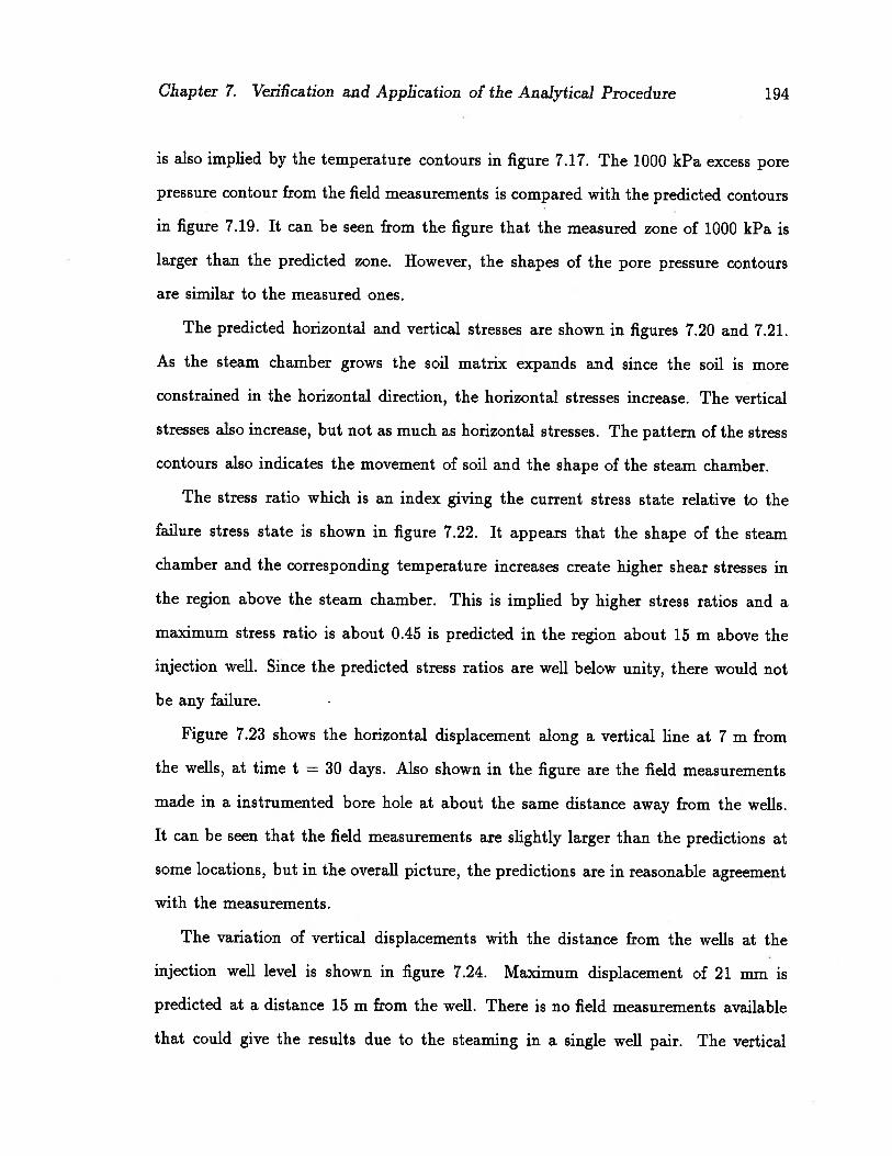
Chapter 7. Verification and Application of the Analytical Procedure 194
is also implied by the temperature contours in figure 7.17. The 1000 kPa excess pore
pressure contour from the field measurements is compared with the predicted contours
in figure 7.19. It can be seen from the figure that the measured zone of 1000 kPa is
larger than the predicted zone. However, the shapes of the pore pressure contours
are similar to the measured ones.
The predicted horizontal and vertical stresses are shown in figures 7.20 and 7.21.
As the steam chamber grows the soil matrix expands and since the soil is more
constrained in the horizontal direction, the horizontal stresses increase. The vertical
stresses also increase, but not as much as horizontal stresses. The pattern of the stress
contours also indicates the movement of soil and the shape of the steam chamber.
The stress ratio which is an index giving the current stress state relative to the
failure stress state is shown in figure 7.22. It appears that the shape of the steam
chamber and the corresponding temperature increases create higher shear stresses in
the region above the steam chamber. This is implied by higher stress ratios and a
maximum stress ratio is about 0.45 is predicted in the region about 15 m above the
injection well. Since the predicted stress ratios are well below unity, there would not
be any failure.
Figure 7.23 shows the horizontal displacement along a vertical line at 7 m from
the wells, at time t = 30 days. Also shown in the figure are the field measurements
made in a instrumented bore hole at about the same distance away from the wells.
It can be seen that the field measurements are slightly larger than the predictions at
some locations, but in the overall picture, the predictions are in reasonable agreement
with the measurements.
The variation of vertical displacements with the distance from the wells at the
injection well level is shown in figure 7.24. Maximum displacement of 21 mm is
predicted at a distance 15 m from the well. There is no field measurements available
that could give the results due to the steaming in a single well pair. The vertical

CD I.
0 CD CD Cl)
U)
I- CD 0 U) CD 0 C,,
CD
EIevL
on
(m)
-01
EIev
Lo
nC
m)
NJ
NJ
-N01
NJ
0U Cl
)
C-,
D C) CD 3
NJ
0
U Co C—,
D 0 CD 3
NJ
0
EIevL
on(rn)
I.U Cl) C
-, 0 CD 3
01 001 0
01 &
c3 0cJ
c30
0CC
)01
Chapter 7. Verification and Application of the Analytical Procedure 196
50
S
40C
0
1::60
Figure 7.19: Comparison of Pore Pressures in the Oil Sand Layer
displacement measurements were made in bore holes located in between the well
pairs and therefore, those measurements cannot be considered as the result due to
the steaming from a single well pair. Moreover, those measurements were very erratic
and a definite pattern of vertical displacements could not be inferred.
The total quantity flow with time at the production well is shown in figure 7.25.
The flow rate increases with time and it can be said that a steady state condition is
achieved after 20 days. The predicted steady state flow rate is 5.18m3/m/day. In the
initial stages of production, more water will be produced than oil because much of
the bitumen will be immobile. With time, the temperature will increase, the viscosity
of bitumen will reduce, it will become mobile and more bitumen will be produced.
As the oil recovery process continues at the steady state conditions, eventually, the
amount of bitumen produced will become less as it is replaced by water.
0 10 20 30 40 50
DsLncG (m)
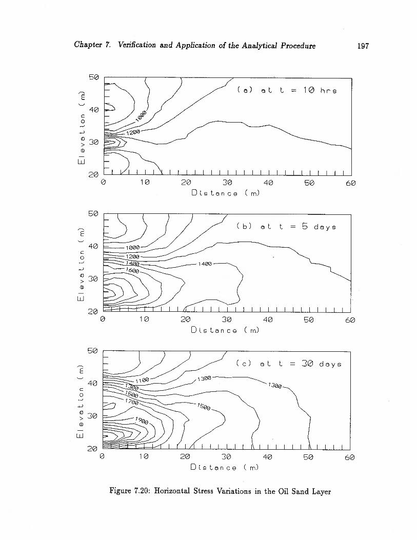
oq CD 0 N 0 C,)
I- CD
EevoL
on
(m)
NJNJ
-01
EIe
v3
Lo
n(m
)N
)N
J-
01
0
0
C,,
E3 C) CD 3
NJ
0
C,)
C-, a, :3 0 CD 3
NJ
0
ci) C)
0) :3 0 CD
EIevL
on
(m)
N)
NJ
-01
00
00
NJ
0
01 0
3
(ii
0(i
i0
c3 00
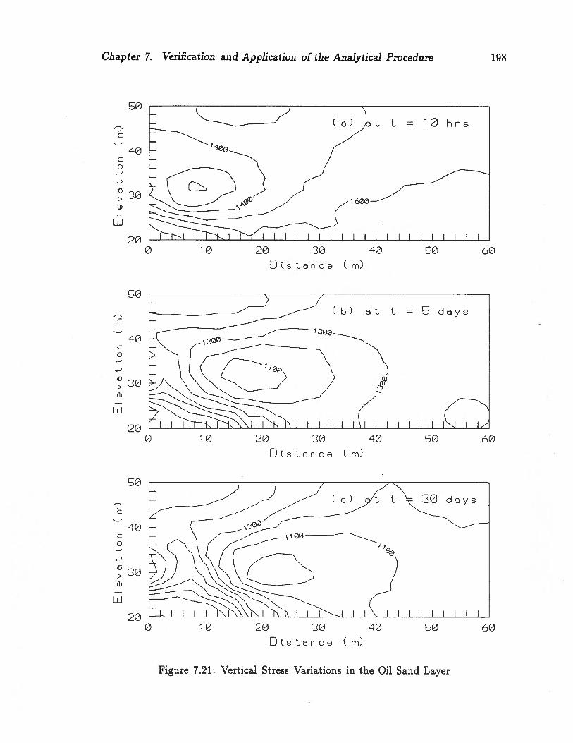
Chapter 7. Verification and Application of the Analytical Procedure 198
- () t tlOhrs
40C
0
/6ØO30
LU
20 I
Dstance (m)0 10 20 30 40 50 60
C
0
30
LU
40
200 10 20 30
D9Lance (m)40
40
E
C
0
>30
20•10 20
DLnce (m)40 60
Figure 7.21: Vertical Stress Variations in the Oil Sand Layer
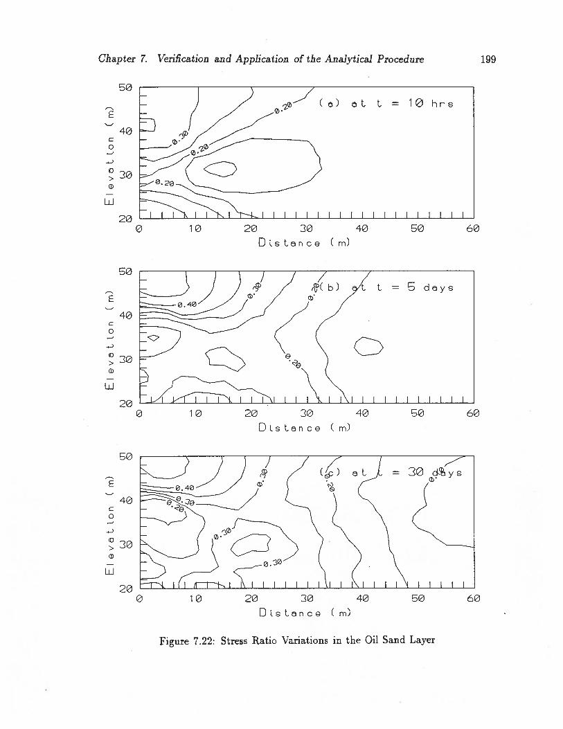
Chapter 7. Verification and Application of the Analytical Procedure 199
60
60
60
40
0
10 20 30 40
DsLance (m)
40C
0
30
Li
200 10 20 30
DLence (m)
40
40C
0
30
Li
200 10 20 30
DLncG (m)
40
Figure 7.22: Stress Ratio Variations in the Oil Sand Layer
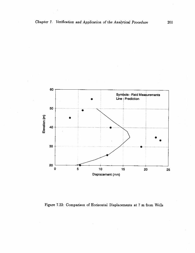
Chapter 7. Verification and Application of the Analytical Procedure 200
60Symbols - Field Measurements
• Line - Prediction
50 •
•0
••
20 I I I I0 5 10 15 20 25
Displacement (mm)
Figure 7.23: Comparison of Horizontal Displacements at 7 m from Wells

Chapter 7. Verification and Application of the Analytical Procedure 201
25
20
E15
10
5
0
600 10 20 30 40 50
Distance (m)
Figure 7.24: Vertical Displacements at the Injection Well Level
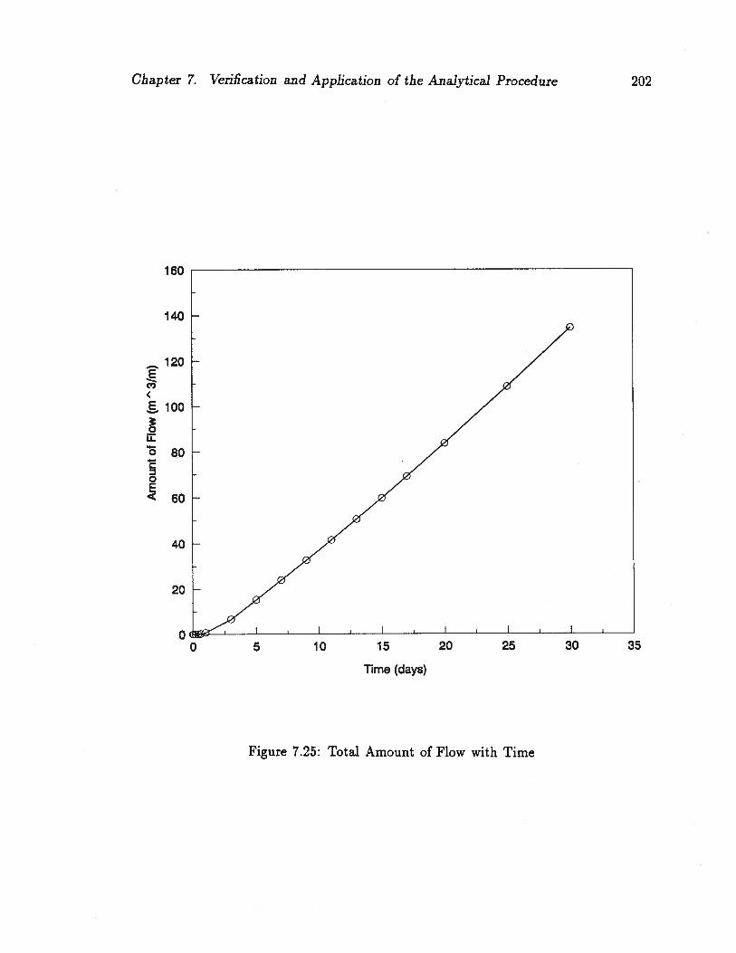
Chapter 7. Verification and Application of the Analytical Procedure
160
140
120
C,,
100
0U.
o 80C
0E<60
40
20
0
Time (days)
202
0 5 10 15 20 25 30 35
Figure 7.25: Total Amount of Flow with Time
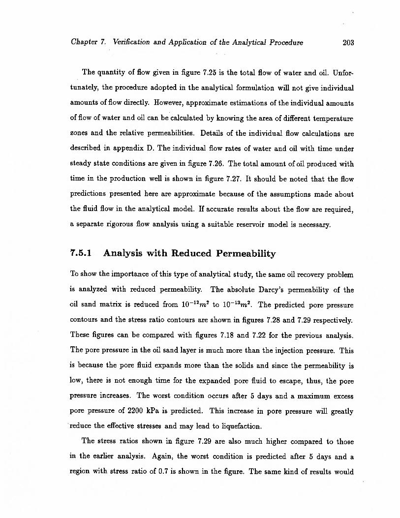
Chapter 7. Verification and Application of the Analytical Procedure 203
The quantity of flow given in figure 7.25 is the total flow of water and oil. Unfor
tunately, the procedure adopted in the analytical formulation will not give individual
amounts of flow directly. However, approximate estimations of the individual amounts
of flow of water and oil can be calculated by knowing the area of different temperature
zones and the relative permeabilities. Details of the individual flow calculations are
described in appendix D. The individual flow rates of water and oil with time under
steady state conditions are given in figure 7.26. The total amount of oil produced with
time in the production well is shown in figure 7.27. It should be noted that the flow
predictions presented here are approximate because of the assumptions made about
the fluid flow in the analytical model. If accurate results about the flow are required,
a separate rigorous flow analysis using a suitable reservoir model is necessary.
7.5.1 Analysis with Reduced Permeability
To show the importance of this type of analytical study, the same oil recovery problem
is analyzed with reduced permeability. The absolute Darcy’s permeability of the
oil sand matrix is reduced from 10’2m2 to 1013m2. The predicted pore pressure
contours and the stress ratio contours are shown in figures 7.28 and 7.29 respectively.
These figures can be compared with figures 7.18 and 7.22 for the previous analysis.
The pore pressure in the oil sand layer is much more than the injection pressure. This
is because the pore fluid expands more than the solids and since the permeability is
low, there is not enough time for the expanded pore fluid to escape, thus, the pore
pressure increases. The worst condition occurs after 5 days and a maximum excess
pore pressure of 2200 kPa is predicted. This increase in pore pressure will greatly
• reduce the effective stresses and may lead to liquefaction.
The stress ratios shown in figure 7.29 are also much higher compared to those
in the earlier analysis. Again, the worst condition is predicted after 5 days and a
region with stress ratio of 0.7 is shown in the figure. The same kind of results would
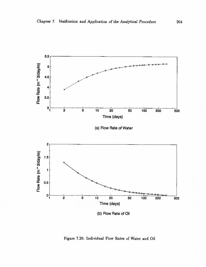
Chapter 7. Verification and Application of the Analytical Procedure 204
•.8
-
Ia)
0U
Ea)
0U-
5.5
5
4.5
4
3.5
2
1.5
1
0.5
01
2 5 10 20 50 100 200 500
Time (days)
(a) Flow Rate of Water
20
Time (days)
(b) Flow Rate of Oil
500
Figure 7.26: Individual Flow Rates of Water and Oil

Chapter 7. Verification and Application of the Analytical Procedure
E
CE
0Li.
0
0E
,2
205
350
50
40
30
20
0 50 100 150 200 250 300
Time (days)
Figure 7.27: Total Amount of Oil Flow
Co C-,
D D C) CD
U Co C-,
D C) CD 3
EIev
ton
(m)
RDRD
-01
RDRD
-R01
EIev
Lo
n(m
)F—
(L
HevL
on
cmRD
RD-
(ii
‘SC‘SC
‘SC
0CD —
3
co
0 CD fri CD Cl)
fri CD 0 ‘-I
U) I-. Cl)
r\D 0
RD 0
3
RD 0
U C/) C-,
Z3 0 (0 3
RD 0
I01 0
01 001 0
0

Chapter 7.
C
0
30
LU
S
C
0
30a)
LU
S
C
0
30
LU
Verification and Application of the Analytical Procedure 207
60
60
60
Figure 7.29: Stress Ratio Variation for Analysis 2
40
200 10 20 30
DtLnce (m)
40
40
200 10 20
DsLncG (m)
30 40
40
200 10 20
DLance (m)40

Chapter 7. Verification and Application of the Analytical Procedure 208
have been predicted if the permeability was kept the same and the rate of heating
increased. The detailed results show that the stress ratio of one of the elements in
the highest stress ratio region reached unity indicating shear failure. Since the region
of shear failure is small and away from the wells, it will not cause any problems.
However, if the region of shear failure is large, there will be significant deformations
and if the region extends to the wells, it may cause significant damage to the wells.
To avoid this kind of situation, the rate of heating should be reduced.
The above example illustrates the usefulness of this type of analytical treatment
for oil recovery projects. This type of analysis provides important information about
the rate of heating, possible failure zones, deformations, stability of the wells etc.,
beforehand. Without an analytical treatment, these concerns have to be tested in the
field on a trial and error basis, which would be very costly.
7.6 Other Applications in Geotechnical Engineering
Even though the finite element program CONOIL was developed for analyzing prob
lems related to oil sands, it can also be applied to other potential geotechnical prob
lems. An example problem which involves pore pressure migration after liquefaction
is described herein.
Generally, loose sands are susceptible to liquefaction in the event of an earthquake
and to prevent such liquefaction, loose sand deposits are commonly densified. The
densified zone in a loose sand deposit will only be stable provided high excess pore
pressures from the surrounding liquefied sands do not penetrate it during and after
the earthquake. This concern is examined herein with different densification schemes
used in practice.
A typical soil profile for Richmond, British Columbia, was considered in the anal
ysis. The soil profile comprised 3 m of clay crust, underlain by 15 m of loose sand and
followed by 5 m of dense sand as shown in figure 7.30. The earthquake is assumed to
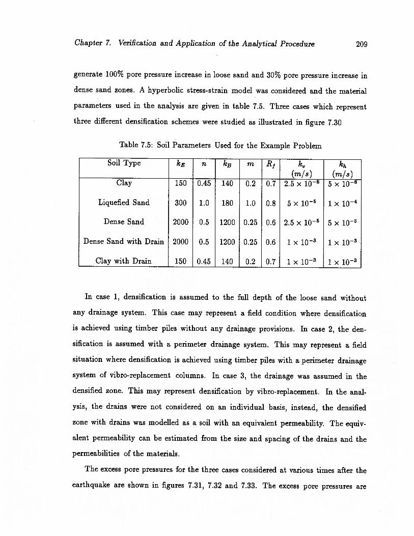
Chapter 7. Verification and Application of the Analytical Procedure 209
generate 100% pore pressure increase in loose sand and 30% pore pressure increase in
dense sand zones. A hyperbolic stress-strain model was considered and the material
parameters used in the analysis are given in table 7.5. Three cases which represent
three different densification schemes were studied as illustrated in figure 7.30
Table 7.5: Soil Parameters Used for the Example Problem
Soil Type n kB m R1 k,, kh(m/s) (m/s)
Clay 150 0.45 140 0.2 0.7 2.5 x 10 5 x iO
Liquefied Sand 300 1.0 180 1.0 0.8 5 X 1O 1 X 10
Dense Sand 2000 0.5 1200 0.25 0.6 2.5 x 10 5 x iO
Dense Sand with Drain 2000 0.5 1200 0.25 0.6 1 x 10 1 x iO
Clay with Drain 150 0.45 140 0.2 0.7 1 x iO 1 x 1O
In case 1, densification is assumed to the full depth of the loose sand without
any drainage system. This case may represent a field condition where densification
is achieved using timber piles without any drainage provisions. In case 2, the den
sification is assumed with a perimeter drainage system. This may represent a field
situation where densification is achieved using timber piles with a perimeter drainage
system of vibro-replacement columns. In case 3, the drainage was assumed in the
densified zone. This may represent densification by vibro-replacement. In the anal
ysis, the drains were not considered on an individual basis, instead, the densified
zone with drains was modelled as a soil with an equivalent permeability. The equiv
alent permeability can be estimated from the size and spacing of the drains and the
permeabilities of the materials.
The excess pore pressures for the three cases considered at various times after the
earthquake are shown in figures 7.31, 7.32 and 7.33. The excess pore pressures are

r0r0
NC
)-O
0CD
0
0 CD ()0.
. .o. CD CD 0
0 3

Chapter 7. Verification and Application of the Analytical Procedure 211
shown in terms of pore pressure ratio u/o0, in which u is the current excess pore
pressure, and o is the initial vertical effective stress. u/a0 = 0 represents zero pore
pressure rise and u/o0 = 1 represents 100% pore pressure rise or liquefaction. The
variations of the excess pore pressure ratios with time and distance from the centre
of the densified zone are shown in graphs (a) and (b) in the figures. Graph (a) shows
the variation at a depth of 5 m and graph (b) at a depth of 10 m. Graph (c) shows
the excess pore pressure ratio with depth along the centre line.
The results for case 1. (figure 7.31) show that the excess pore pressure in the
surrounding undensified area migrates into the densified zone. The pore pressure
ratio in the upper part of the densified zone rises to 1 which means liquefaction
will be triggered. However, below a depth of 6 m, liquefaction is not triggered and
piles penetrating below this depth could support vertical load, although significant
horizontal displacements are likely to occur. The results for case 2 (figure 7.32)
indicate that a perimeter drainage system is quite effective in preventing the migration
of high pore pressure from the loose zone into the densified zone. A maximum pore
pressure ratio of 0.5 is predicted 1 mm after the earthquake. The results for case 3
where the drainage is assumed throughout the densified zone are shown in figure 7.33.
It can be seen from the figure that the drains in the densified zone are much more
effective in preventing the migration of pore pressure in the densified zone. The pore
pressure ratio in the densified zone increases from an initial value of 0.3 at time t =
0, to 0.4 after 10 seconds and then reduces.
The conclusions from the analyses are as follows. Densification alone such as could
be achieved by driving timber piles will not prevent the high excess pore pressures
from the surrounding liquefied zone penetrating the densified zone. Such penetration
will cause liquefaction to a depth of 6 m for the conditions analyzed. Below this depth
effective stress increases and timber piles would be capable of carrying vertical load
although they could be damaged by horizontal movements. Perimeter drains could
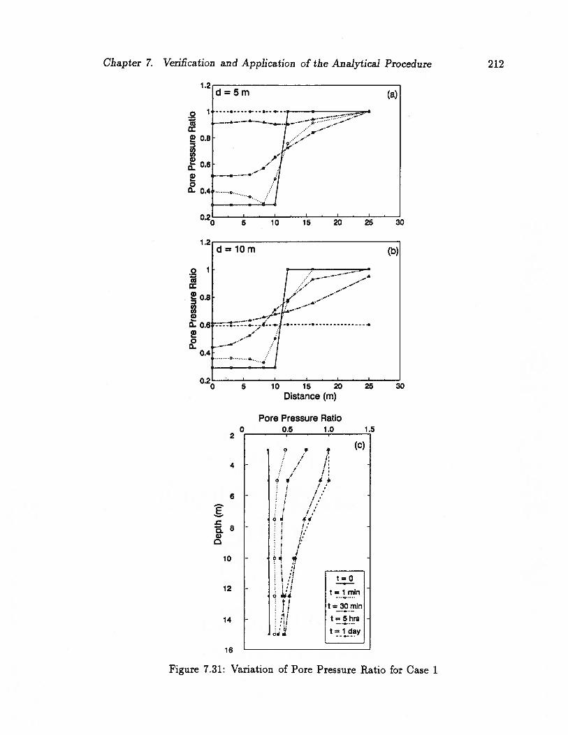
Chapter 7. Verification and Application of the Analytical Procedure 212
1.2d=5m (a)
30
d=lOm (b)
0.8
Distance (m)
Pore Pressure Ratio0 0.5 1.0 1.5
2
•(c)
4- Si, /di’
6- / /z’
!e
I,,
10 - QI
I/i12 - ‘:1 t=lmin
t=3Ornin
14 -t5hrs
t =lday
16
Figure 7.31: Variation of Pore Pressure Ratio for Case 1
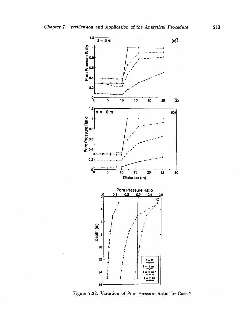
Chapter 7. Verification and Application of the Analytical Procedure 213
1.2d=5m (a)
d=lOm (b)
c05 10 15 20 25 30
Distance (m)
Pore Pressure Ratio0 0.1 0.2 0.3 0.4 0.
L(C)
4- //
A 0
: :: :b-f
12- 1 1 t=o4 1
t=lmin
14- t5rflifl
I t=5hr
______________
I
______
1€
Figure 7.32: Variation of Pore Pressure Ratio for Case 2
Chapter 7. Verification and Application of the Analytical Procedure 214
d=5m (a)
t=rnin
15 20 30
1.2d=lOm (b)
__
30
Distance (m)
Pore Pressure Ratio0 0.1 0.2 0.3 04
(C)7
4-
4I
G)0 /
10- 4
12- 1t 9
14-
0
Figure 7.33: Variation Of Pore Pressure Ratio for Case 3

Chapter 7. Verification and Application of the Analytical Procedure 215
greatly reduce the migration of excess pore pressures into the densified zone. The
provision of drainage within the densifled zone can be very effective in preventing
high excess pore pressures in the densifled zone.
A more detailed study of this problem including the effect of densification depth
is presented in Byrne and Srithar (1992). Some other applications of the program
can be found in Byrne et al. (1991a), Byrne et al. (1991b), Jitno and Byrne (1991)
and Crawford et al. (1993).

Chapter 8
Summary and Conclusions
An analytical procedure is presented to analyze the geotechnical aspects in an oil
recovery process from oil sand reserves. The key issues in developing an analytical
model are: the stress-strain behaviour of the sand skeleton; the behaviour of the
three-phase pore fluid; and the effects of temperature changes associated with steam
injection. A coupled stress-deformation-flow model incorporating these key issues is
presented in this thesis.
In modelling the stress-strain behaviour of the oil sand skeleton, shear induced
dilation is an important aspect. Such dilation can increase the hydraulic conductivity
and hence increase oil recovery. Dilation will also lead to reduced pore fluid pressure
and increased stability. The other pertinent aspect is the stress-strain response un
der stress paths involving a decrease in mean stress under constant shear stress and
loading-unloading cycles. The stress-strain models used in the current-state-of-the-
practice are linear or nonlinear elastic models which are incapable of modelling the
above mentioned aspects realistically. The major contribution of this thesis is the
development of a suitable elasto-plastic stress-strain model to capture the important
aspects. The stress-strain model postulated in this thesis is a double hardening type
consisting two yield surfaces. The model has a cone-type yield surface to predict
shear induced plastic strains and a cap-type yield surface to predict volumetric plas
tic strains. The predictions from the stress-strain model have been compared with
laboratory test results under various types of loading and are in good agreement. The
dilation, plastic strains due to cyclic loading, and the response under different stress
216

Chapter 8. Summary and Conclusions 217
paths have been well predicted by the stress-strain model.
The pore fluid in oil sand comprises water, bitumen and gas and the three-phase
nature of the pore fluid has to be recognized in modelling the behaviour of pore fluid.
In petroleum reservoir engineering, multiphase fluid flow is modelled by elaborate
multiphase thermal simulators. In this study, the effects of multiphase pore fluid
are modelled through an equivalent single phase fluid. An effective flow continuity
equation is derived from the general equation of mass conservation which is one
of the other contributions of this thesis. An equivalent compressibility term has
been derived by considering the individual contributions of the phase components.
Compressibility of gas has been obtained from gas laws. An equivalent hydraulic
conductivity term has been derived by considering the relative permeabilities and
viscosities of the individual phases in the pore fluid. The relative permeabilities have
been assumed to vary with saturation and the viscosities have been assumed to vary
with temperature and pressure. Gas exsolution which would occur when the pore fluid
pressure decreases below the gas/liquid saturation pressure has also been modelled.
Oil recovery schemes commonly involve some form of heating and therefore, tem
perature effects on the sand skeleton and pore fluid behaviour are important. Changes
in temperature will cause changes in viscosity, stresses and pore pressures and con
sequently in some of the engineering properties such as strength, compressibility and
hydraulic conductivity. In this study, the stress-strain relation and the flow conti
nuity equation have been modified to include the temperature induced effects. This
approach of including the temperature effects directly in the governing equations gave
very stable results, compared to the general thermal elastic approach.
The final outcome of this research work is a finite element program which incorpo
rates all the above mentioned aspects. The new stress-strain model, flow continuity
equation, and other related aspects have been incorporated in the existing two di
mensional finite element program CONOIL-Il. This required significant undertakings

Chapter 8. Summary and Conclusions 218
including a new solution routine as the new stress-strain model results in an unsym
metric stiffness matrix. A frontal solution technique which requires less computer
memory has been employed to solve the resulting equations. A new three dimen
sional finite element program has also been developed following the same concepts.
The validity of the finite element codes has been checked for various aspects by com
paring the program predictions with closed form solutions and laboratory results.
The predicted results agreed very well with the closed form solutions and laboratory
results.
The two dimensional finite element code has been applied to model a horizontal
well pair in the underground test facility of AOSTRA. Results have been presented in
terms of displacements, stresses, stress ratios and amounts of flow and discussed. The
measured and predicted results have been compared wherever possible and they agree
well. A method to obtain individual amounts of flow of the pore fluid components
has also been devised.
The type of analytical study presented in this thesis, is very important in oil
recovery projects, since it could give insights into the likely behaviour in terms of
stresses, deformations and flow. For instance, the permeability of the oil sand and
the rate of heating due to steam injection have been examined in some detail. It
has been revealed that in oil sands with low permeability, higher rates of heating
would cause shear failure. If the local shear failure zone extends to the wellbore it
could cause significant damage. Information of this kind would be beneficial to the
successful operation of an oil recovery scheme.
Although the finite element program has been developed to analyze the problems
related to oil sand specifically, it can be applied to other geotechnical problems. To
demonstrate its applicability, a problem involving pore pressure redistribution after
liquefaction has been analyzed and the results are discussed.

Chapter 8. Summary and Conclusions 219
8.1 Recommendations for Further Research
Following the work presented in this study, some aspects can be identified in this
area which require further study. Application of the finite element codes to more
oil recovery problems should be carried out to increase the credibility of the models.
The three dimensional code is newly written and even though various aspects of the
code have been verified, it has not been applied to analyze a oil recovery problem of
a three dimensional nature. The three dimensional code needs to be applied to either
a physical model test or a field problem where the responses are measured, in order
to check its capability to model three dimensional effects.
Even though the analytical formulation presented in this study includes the effects
of multi-phase fluid through equivalent compressibility and hydraulic conductivity
terms, it does not take the flow of thermal energy into account. Incorporation of
an elaborate multi-phase thermal and fluid flow model would be the most desired
enhancement though it may be a very difficult task. Previous researchers concluded
that analyzing the geomechanical behaviour and the thermal and fluid flow behaviour
separately, and combining the results by partial coupling is useful and successful.
However, a fully integrated analytical formulation may be more efficient.
Perhaps another aspect which require further study would be the stress-strain
model for the sand skeleton. The elasto-plastic stress-strain model described in this
study does not consider anisotropy effects. Modelling strain softening by load shed
ding may also be inefficient since it requires a large number of iterations. A stress
strain model which includes anisotropy and strain softening effects in a realistic man
ner is worth considering.
Fractures in the oil sand layer are sometimes encountered in the oil recovery
process by steam injection. Inclusion of modelling of fracture initiation and its prop
agation will also be beneficial.

Bibliography
[1] Aboshi, H., Yoshikuni, H. and Maruyama, S. (1970), “Constant Load
ing Rate Consolidation Test”, Soils and Foundation, vol. X, No. 1, pp 43-56.
[2] Aboustit, B.L., Advani, S.H., Lee, J.K. and Sandu, R.S. (1982),
Finite Element Evaluation of Thermo-Elastic Consolidation”, Issues on Rock
Mech., 23rd Sym. on Rock Mech., Univ. of California, Berkeley, pp 587-595.
[3] Aboustit, B.L., Advani, S.H. and Lee, J.K. (1985), “Variational Prin
ciples and Finite Element Simulations for Thermo-Elastic Consolidation”, mt.J. for Num. and Anal. Mtds. in Geomech., Vol. 9, pp 49-69.
[4] Adachi, T. and Okamo, M. (1974), “A Constitutive Equation for Normally
Consolidated Clay “, Soils and Foundations, Vol. 14, No.4, pp 55-73.
[5] Agar, J.G., Morgenstern, N.R. and Scott, J.D. (1987), “Shear Strength
and Stress Strain Behaviour of Athabasca Oil Sand at Elevated Temperatures
and Pressures”, Can. Geotech. J., No. 24, pp 1-10.
[6] Agar, J.G., Morgenstern, N.R. and Scott, J.D. (1986), “Thermal Ex
pansion and Pore Pressure Generation in Oil Sands”, Can. Geotech. J., Vol.
23, pp 327-333.
[7] Akin, J.E. and Pardue, R.M. (1975), “ Element Resequencing for Frontal
Solutions”, The Mathematics of Finite Elements and Applications, Ed: White
man, J.R., Academic Press, London, pp 535-54 1.
220

Bibliography 221
[8] Aziz, K. and Settari, T. (1979), “ Petroleum Reservoir Simulation “, Ap
plied Science Publ., London.
[9] Baker, L.E. (1988), “Three-Phase Relative Permeability Correlations “, SPE
Paper No. 17369, SPE/DOE EOR Symp., Tulsa, Okiakoma.
[10] Bathe, K. and Wilson, E.L. (1976), “Numerical Methods in Finite Element
Analysis”, Pub. by Prentice Hall.
[11] Blot, M.A. (1941), “General Theory of Three Dimensional Consolidation”,
J. of App. Physics, Vol. 12, pp 155-164.
[12] Blot, M.A. (1941(b)), “Consolidation Under a Rectangular Load Distribu
tion”, J. of App. Physics, Vol. 12, pp 426-430.
[13] Bishop, A.W. (1973), “ The Influence of an Undrained Change in Stress
on The Pore Pressure in Porous Media of Low Compressibility”, Geotechnique,
Vol. 23, No. 3, pp 4 35-442.
[14] Bishop,A.W. and Henkel, D.J. (1957), “The Measurements of Soil Prop
erties in The Triaxial Test”, 2nd Ed., William Arnold Pub 1., U.K.
[15] Booker, J.R. (1974), “The Consolidation of a Finite Layer Subject to Surface
Loading”, mt. J. of Solids Structures, Vol. 10, pp 1053-65.
[16] Booker, J.R. and Small, J.C. (1975), “ An Investigation of the Stability
of Numerical Solutions of Biot’s Equations of Consolidation”, mt. J. of Solids
and Structures, Vol. 11, pp 907-917.
[17] Booker, J.R. and Savvidov, C. (1985), “ Consolidation Around a Point
Heat Source”, mt. J. for Num. and Anal. Mtds. in Geomech., Vol. 9, pp 173-
184.

Bibliography 222
[18] Byrne, P.M. (1983), “ Static Finite Element Analysis of Soil Structure
Systems”, Soil Mech. Series, No. 71, Dept. of Civil Eng., Univ. of British
Columbia, Vancouver, Canada.
[19] Byrne, P.M. and Cheung, H. (1984), “ Soil Parameters for Deformation
Analysis of Sand Masses”, Soil Mech. Series, No. 81, Dept. of Civil Eng., Univ.
of British Columbia, Vancouver, Canada.
[20] Byrne, P.M. and Eldridge, T.L. (1982), “ A Three Parameter Dilatant
Elastic Stress-Strain Model for Sand”, mt. Sym. on Num. Mtds. in Geomech.,
Switzerland, pp 78-79.
[21] Byrne, P.M. and Grigg, R.G. (1980), “ OILSTRESS - A Computer Pro
gram for Analysis of Stresses and Deformations in Oil Sand “, Soil Mech. Series,
No. 42, Dept. of Civil Eng., Univ. of British Columbia, Vancouver, Canada.
[22] Byrne, P.M. and Janzen, W. (1984), “INCOIL- A Computer Program for
Nonlinear Analysis of Stress and Deformation of Oil Sand Masses”, Soil Mech.
Series, No. 80, Dept. of Civil Eng., Univ. of British Columbia, Vancouver,
Canada.
[23] Byrne, P.M. and Srithar, T. (1992), “Assessment of Foundation Treatment
for Liquefaction “ First Can. Symp. on Geotechnique and Natural Hazards,
Vancouver, B. C.
[24] Byrne, P.M., Skermer, N. and Srithar T. (1991a), “ Uplift Pressures
Due to Liquefaction of Sediments Stored Behind Concrete Dams “ 3rd Annual
Conf of the Can. Dam Safety Assoc., Whistler, B.C., pp 149-168.
[25] Byrne, P.M., Srithar, T. and Yan L. (1991b), “ Effects of Earthquake
Induced Liquefaction of Soils Stored Behind Concrete Dams “ 2nd mt. Conf
on Geotech. Earthquake Engr. and Soil Dynamics, Missouri Rolla.

Bibliography 223
[26] Byrne, P.M., Cheung, H. and Yan L. (1987), “Soil Parameters for Defor
mation Analysis of Sand Masses “, Can. Geotech. J, Vol. 24, No. 3, pp 366-376.
[27] Byrne, P.M., Vaid, Y.P. and Samerasekera, L. (1982), “ Undrained
Deformation Analysis Using Path Dependent Material Properties”, mt. Sym.
on Num. Mtds. in Geomech., Switzerland pp 294-302.
[28] Byrne, P.M. and Vaziri, H.H. (1986), “CONOIL: A Computer Program
for Nonlinear Analysis of Stress Deformation and Flow in Oil Sand Masses”,
Soil Mech. Series, No. 103, Dept. of Civil Eng., Univ. of British Columbia,
Vancouver, Canada.
[29] Campanella, R.G. and Mitchell, K.J. (1968), “Influence of Temperature
Variations on Soil Behaviour”, J. of SMFD, ASCE, Vol. 94, SM 3, pp 709-734.
[30] Carr, N.L., Kobayashi, R. and Burrows, D.B. (1954), “ Viscosity of
Hydrocarbon Gases under Pressure “, Trans. AIMME, Vol. 201, pp 264-272.
[31] Carter, J.P. (1977), “ Finite Deformation Theory and its Application to
Elasto-Plastic Soils”, Ph.D. Thesis, University of Sydney, Australia.
[32] Chang, C.S. and Duncan, J.M. (1983), “Consolidation Analysis for Partly
Saturated Clay Using An Elasto-Plastic Effective Stress-Strain Model”, mt. J.
for Num. and Anal. Mtds. in Geomech., Vol. 17 pp 39-55.
[33] Chen, W.F. (1982), “Plasticity in Reinforced Concrete “, McGraw Hill New
York, NY.
[34] Cheung, H.K.F. (1985), “ A Stress-Strain Model for The Undrained Re
sponse of Oil Sand”, M.A.Sc Thesis, Dept. of Civil Eng., Univ. of British
Columbia, Vancouver, Canada.

Bibliography 224
[35] Christian, J.T. and Boehmer,J.W. (1970), “Plane Strain Consolidation
by Finite Elements”, J. of SMFD, ASCE, Vol. 96, SM4, pp 1435-57.
[36] Crawford, C.B., Jitno, H. and Byrne P.M. (1993), “The Influence of Lat
eral Spreading on Settlements Beneath a Fill “ to be published in Can. Geotech.
J.
[37] Drucker, D.C., Gibson, R.E. and Henkel, D.J. (1955), “Soil mechanics
and Work-Hardening Theories of Plasticity “, Proceedings, ASCE, Vol.81, pp
1-14.
[38] Duncan, J.M. and Chang, C.Y. (1970), “Nonlinear Analysis of Stress and
Strain in Soils”, J. of SMFD, ASCE, Vol. 96, SM 5, pp 1629-1651.
[39] Duncan, J.M., Byrne, P.M., Wong, K.S. and Mabry, P. (1980)
Strength, Stress-Strain and Bulk Modulus Parameters for Finite Element Anal
yses of Stresses and Movements in Soil Masses”, Report No. UCB/GR/78-02,
Dept. of Civil Engr., Univ. of California, Berkeley.
[40] Dusseault, M.B. (1980), “ Sample Disturbance in Athabasca Oil Sand”, J.
of Can. Petroleum Tech., Vol. 19, pp 85-92.
[41] Dusseault, M.B. (1979), “Undrained Volume and Stress Change Behaviour
of Unsaturated Very Dense Sands”, Can. Geotech. J., Vol. 16, pp 627-640.
[42] Dusseault, M.B. (1977), “ The Geotechnical Characteristics of Athabasca
Oil Sands “, Ph.D Thesis, Dept. of Civil Engr., Univ. of Alberta, Canada.
[43] Dusseault, M.B. and Morgenstern, R.N. (1978), “ Characteristics of
Natural Slopes in the Athabasca Oil Sands “, Can. Geotech. J., Vol. 15, pp
202-215.

Bibliography 225
[44] Dusseault, M.B. and Rothenburg, L. (1988), “Shear Dilatancy and Per
meability Enhancement in Oil Sands “, Paper No. 82, 4th UNITAR/UNDP mt.Conf. on Heavy Crude and Tar Sands.
[45] Dusseault, M.B. and Van Domselaar, H.R. (1982), “ Canadian and
Venezuelan Oil Sand: Problems and Analysis of Uncemented Gaseous Sand
Sampling”, Proc. of the Engr. Found. Conf on Updating Subsurface Sampling
of Soils and Rocks and Their In-Situ Testing, Santa Barbara, California.
[46] Edmunds, N.R., Wong, A. McCormack, M.E. and Sugget, J.C.
(1987), “Design of Horizontal Well Completions - AOSTRA Underground Test
Facility “, 4th Annual Heavy Oil and Oil Sand Symposium, U. of Calgary, Paper
No. 2.
[47] Ewing, R.E (1989), “Finite Elements in Reservoir Simulation”, Proc. of the
7th mt. Conf on FEM in Flow Problems, U. of Alabama, pp 1251-1257.
[48] ERCB (1975), “The Theory and Practice of the Testing of Gas Wells “, 3rd
Edn., Energy Resources Conservation Board.
[49] Faust, C.R. and Mercer, J.W. (1976), “ An Analysis of Finite-Difference
and Finite Element Techniques for Geothermal Reservoir Simulation”, SPE
5742.
[50] Finol, A. and Farouq Au, S.M. (1975), “ Numerical Simulation of Oil
Production with Simultaneous Ground Subsidence “, SPEJ 411.
[51] Frantziskonis, G. and Desai, C.S. (1987a), “ Constitutive Model with
Strain Softening “, mt. J. Solids Structures, Vol. 23, No. 6, pp 733-750.
[52] Frantziskonis, G. (1986), “Progressive Damage and Constitutive Behaviour
of Geomaterials Including Analysis and Implementation “ Ph.D Thesis, Dept.
Bibliography 226
of Civil Engr., U. of Arizona, Tucson) Arizona.
[53] Frantziskonis, G. and Desai, C.S. (1987b), “Analysis of a Strain Softening
Constitutive Model “, mt. J. Solids Structures, Vol. 23 No. 6, pp 751-767.
[54] Fredhind, D.G. (1973), “ Discussion: Flow and Shear Strength”, Proc. of
3rd mt. Conf on Expansive Soils, Haifa, Vol. 2, pp 71-76.
[55] Fredlund, D.G. (1976), “Density and Compressibility Characteristics of Air
Water Mixtures”, Can. Geotech. J., Vol. 13, pp 386-396.
[56] Fredlund, D.G. (1979), “ Appropriate Concepts and Technology for Unsat
urated Soils”, Can. Geotech. J., Vol. 16, pp 121-139.
[57] Fredlund, D.G. and Morgenstern, N.R. (1977), “ Stress State Variables
for Unsaturated Soils”, J. of Ceotech. Eng. Div., ASCE, Vol.103, pp 447-466.
[58] Fung, L.S.K. (1990), “ A Coupled Geomechanical Multiphase Flow Model
for Analysis of In-Situ Recovery in Cohesionless Oil Sands “, CIM/SPE 90-29,
CIM/SPE 1990 mt. Tech. Metting, Calgary, Alberta.
[59] Gassman, F. (1951), “ Uber die Elastizitat poroser Medien “, Vierteljahrss
chrift der Naturforschenden Geselishaft in Zurich, Mitteilungen aus dem Insti
tut fur Ceophysik, 171.
[60] Ghaboussi, J. and Kim, K.J. (1982), “ Analysis of Saturated and Partly
Saturated Soils”, mt. Sym. on Num. Mtds. in Geomech., Zurich, pp 377-390.
[61] Ghaboussi, J. and Wilson, E.L. (1973), “Flow of Compressible Fluid in
Porous Elastic Media”, mt. J. for Num. Mtds. in Engr., Vol. 5, pp 4 19-442.
[62] Gibson, R.E., Schiffmann, R.L. and Pu, S.L. (1970), “Plane Strain and
Axisymmetric Consolidation of a Clay Layer on a Smooth Impervious Base”,
Quart. J. of Mech. and Applied Math., Vol. XXIIL Part 4, pp 505-519.
Bibliography 227
[63] Geertsma, J. (1957), “ The Effect of Fluid Pressure Decline on Volumetric
Changes of Porous Rocks “, Pet. Trans., AIME, No. 210, pp 331-340.
[64] Geertsma, J. (1966), “Problems of Rock Mechanics in Petroleum Production
Engineering “, Proc. of the 1st Cong. of li-it. Soci. of Rock Mechanics, Lisbon,
pp 585-594.
[65] Grieg, J., Byrne, P.M. and Srithar, T. (1990), “ COPP - çQnoil Rost
Erocesser, A Software Package for Pre/Post Processing CONOIL Data “, Dept.
of Civil Engr., U. of British Columbia, Vancouver, Canada.
[66] Gudehus, G. and Darve, F., eds (1982), “Proceedings of the International
Workshop on the Constitutive Behaviour of Soils”, Grenoble, France.
[67] Gulbrandsen, S. and Wille, S.O. (1985), “A Finite Element Formulation
of the Two-Phase Flow Equations for Oil Reservoirs “, SPE 13516, 8th SPE
Symp. on Reservoir Simulation, Dallas, Texas.
[68] Harris, M.C. and Sobkowicz, J.C. (1977), “Engineering Behaviour of Oil
Sand”, The Oil Sands of Canada Venezula, The Canadian Inst. of Mining and
Metallurgy, Special Vol. 1’4 pp 270-281.
[69] Hinton, E. and Owen, D.R.J. (1977), “ Finite Element Programming “,
Academic Press, London.
[70] Hood, P. (1976), “ Frontal Solution Program for Unsymmetric Matrices”,
mt. J. for Num. Mtds. in Engineering, Vol. 10, pp 379-399.
[71] Hwang, C.T., Morgenstern, N.R. and Murray, D.W. (1972), “ Ap
plication of Finite Element Method to Consolidation Problems”, Application
of FEM in Geotech. Engr., Proc. of Symp., Vicksburg, Mississippi, Vol. I1 pp
739-765.
Bibliography 228
[72] Hughes, J.M.O., Worth, C.P. and Windle, D. (1977), “ Pressuremeter
Tests in Sands”, Geotechnique, Vol. 27, No. 4, pp 455-477.
[73] Huyakorn, P.S. and Pinder, G.F. (1977a), “Solution of Two-Phase Flow
Using a New Finite Element Technique”, Applied Numerical Modelling, Ed. by
C. A. Brebbia, U. of Southampton, July, pp 375-590.
[74] Huyakorn, P.S. and Pinder, G.F. (1977b), “ A Pressure-Enthalpy fi
nite Element Model for Simulating Hydrothermal Reservoirs “, Advances in
Computer Methods for Partial Differential Equations Il, Ed. by Vichnevetsky,
IMACS (AlGA).
[75] Irons, B.M. (1970), “A Frontal Solution Program for Finite Element Anal
ysis”, mt. J. for Num. Mtds. in Engr., Vol. 2, pp 5-32.
[76] Irons, B.M. and Ahmad, S. (1980), “Techniques of Finite Elements”, Ellis
Horwood, Chichester, U.K.
[77] Iwan, W.D. (1967), “ On a Class of Models for the Yielding Behaviour of
Continuous and Composite Systems “, J. Appl. Mech., Vol.34, pp 612-617.
[78] Javandel, I. and Wtherspoon, P.A. (1968), “ Application of the Finite
Element Method to Transient Flow in Poros Media”, Soc. of Petroleum Engr.
J., Sep., pp 24 1-252.
[79] Jitno, H. and Byrne, P.M. (1991), “ Prediction of Settlement at the Cole-
brook Overpass Using 2-D Finite Element Analysis “, Dept. of Civil Engr.,
Univ. of B. C., Unpublished.
[80] De Josselin de Jong (1957), “Application of Stress Functions to Consolida
tion Problems”, Proc. of the 4th mt. Conf. on Soil Mech. and Found. Engrg.,
London, Vol. 1, pp 320-323

Bibliography 229
[81] Ko, H.Y. and Sture, S. (1981), “State of the art: Data Reduction and Ap
plication for Analytical Modelling “, Laboratory Shear Strength of Soil, ASTM
STP 740, Yong, R.N and Townsend F.C., eds, American Society for Testing
and Materials, pp 329-386.
[82] Kokal, S.L. and Maini, B.B. (1990), “An Improved Model for Estimating
Three-Phase Oil-Water-Gas Relative Permeabilities from Two-Phase Oil-Water
and Oil-Gas Data “, J. Can. Petro. Tech., Vol. 29, No. 2, pp 105-114.
[83] Konder, R.L. (1963), “ Hyperbolic Stress-Strain Response: Cohesive Soils”,
J. of SMFD, ASCE, Vol. 89, SM 1, pp 115-143.
[84] Kosar, K.M. (1989), “ Geotechnical Properties of Oil Sands and Related
Strata”, Ph.D Thesis, Dept. of Civil Eng., Univ. of Alberta, Edmonton, Canada.
[85] Kosar, K.M., Scott, J.D. and Morgenstern, N.R. (1987), “ Testing to
Determine the Geotechnical Properties Oil Sands”, CIM Paper 87-38-59, 38th
ATM of Pet. Soc. of CIM, Calgary.
[86] Lade, P.V. (1987), “ Behaviour of Plasticity Theory for Metals and Fric
tional Materials “, Constitutive Laws for Engineering Materials; Theory and
Applications.
[87] Lade, P.V. (1977), “Elasto-Plastic Stress-Strain Theory for Cohesionless Soil
with Curved Yield Surfaces”, mt. J of Solids Structures, Vol. 13, pp 1019-1035.
[88] Lade, P.V. and Duncan, J.M. (1975), “Elasto-Plastic Stress-Strain Theory
for Cohesionless Soil “, J. of the Geot. Engr. Div, ASCE, Vol. 101.
[89] Laing, J.M., Graham, J.P., Stokes, A.W. and Collins, P.M. (1992),
Geotechnical Instrumentation and Monitored In-Situ Behaviour of Oil Sands

Bibliography 230
During Steaming at the AOSTRA UTF Phase-A Trial” 44th Can. Geot. Conf.,
Vol. 2, Paper No. 89, Calgary.
[90] Lambe, T.W. and Whitman, RN. (1969), “Soil Mechanics “, John Wiley
& Sons.
[91] Leverett, M.C. and Lewis, W.B. (1941), “ Steady Flow of Gas-Oil-Water
Mixtures Through Unconsolidated Sands “, Trans., AIME, Vol.142, pp 107-
116.
[92] Lewis, R.W., Morgan, K. and Roberts, P.M. (1985), “Finite Element
Simulation of Thermal Recovery Process and Heat Losses to Surrounding Strata
“, 3rd European Meeting on Improved Oil Recovery, Rome, April pp 305-315.
[93] Lewis, R.W., White, I.R. and Wood W.L. (1978), “A Starting Algorithm
for the Numerical Simulation of Two-Phase Flow Problems “, IJNME, Vol. 12,
pp 319-328.
[94] Lewis, R.W., Roberts, G.K. and Zienkiewicz, O.C. (1976), “A Nonlin
ear Flow and Deformation Analysis of Consolidation Problems”, 2nd mt. Conf
on Num. Mtds. in Ceomech., Blacksburg, Virginia, Vol.2, pp 1106-1118.
[95] Light, M.F. and Luxmoore, A.R. (1977), “Application of the Front So
lution to Two and Three Dimensional Elasto-Plastic Crack Problems”, mt. J.
for Num. Mtds. in Engrg., Vol. 11, pp 393-395.
[96] Matsuoka, H. (1983), “ Deformation and Strength of Granular Materials
Based on the Theory of Compounded Mobilized Plane and Spatial Mobilized
Plane “, Advances in the Mech. and the Flow of Granular Materials, Trans.
Tech. Publ., pp 813-836.
Bibliography 231
[97] Matsuoka, H. (1974), “ A Microscopic Study on Shear Mechanism of Gran
ular Materials “, J. Soils and Foundations, Vol. 14, No.1, pp 29-43.
[98] Matsuoka, H. and Nakai, T. (1982), “ A New Failure Criterion for Soils
in Three-Dimensional Stresses “, IUTAM Conf on Deformation and Failure of
Granular Materials, Delfi, pp 253-263.
[99] Matsuoka, H. and Nakai, T. (1977), “ Stress-Strain Relationship of Soil
Based on the SMP “, Proc., Speciality Session 9, 9th ICSMFE, pp 153-162.
[100] Matsuoka, H. and Nakai, T. (1974), “ Stress Deformation and Strength
Characteristics of Soil under Three Different Principal Stresses “, Proc., JSCE,
No. 232., pp 59-70.
[101] Mayer, C. (1973), “ Solution of Linear Equations - State of the Art”, J. of
the Struc. Div., ASCE, Vol. 99, ST?, pp 1507-1526.
[102] McMichael, C.L. and Thomas, G.W. (1973), “ Reservoir Simulation by
Galerkin’s Method “, SPEJ, June, pp 125-138.
[103] McNamee, J. and Gibson, R.E. (1960), “Plane Strain and Axially Sym
metric Problems of Consolidation of A Semi-Infinite Clay Stratum”, Quart. J.
of Mech. and Appi. Maths., Vol. 13, pp 210-227.
[104] Mitchel, J.K., Hooper, O.R. and Campanella, R.J. (1965), “ Perme
ability of Compacted Clay”, J. of SMFD, ASCE, Vol. 91, SM 4, pp 4 1-65.
[105] Mosscop, G.D. (1980), “Geology of the Athabasca Oil Sands”, Science, Vol.
207, No.11, pp 145-152.
[106] Murayama, S. (1964), “ A Theoretical Consideration on the Behaviour of
Sand”, Proc. IUTAM Symp. of Rheology and Soil Mech., Grenoble, pp 65-79.

Bibliography 232
[107] Murayama, S. and Matsuoka, H. (1973), “A Microscopic Study on Shear
ing Mechanism of Soils “, Proc. of the 8th ICSMFE, Vol. 1, pp 293-298.
[108] Nakai T. and Matsuoka H. (1983), “Constitutive Equation for Soils Based
on the Extended Concept of Spatial Mobilized Plane and its Application to
Finite Element Analysis” Soils and Foundations, Vol. 23, No.4, pp 87-105.
[109] Naylor, D.J. (1973), “Discussion”, Proc. of The Symp. on The Role of The
Plasticity in Soil Mech., Cambridge, pp 291-294.
[110] Negussey, D. (1984), “An Experimental Study on the Small Strain Response
of Sand “, Ph.D Thesis, Dept. of Civil Engr., U of British Columbia, Vancouver,
Canada.
[111] Nemat-Nasser, S. (1980), “On the Behaviour of Granular Material in Simple
Shearing”, Soils and Foundations, Vol. 20, No.3, pp 59-73.
[112] Nova, R. and Wood D.M. (1979), “ A Constitutive Model for Sand in
Triaxial Compression “, mt. J. for Num, and Anal. Mtds. in Geomechanics,
Vol.3.
[113] Oda, M. and Konishi, J. (1974), “Microscopic Deformation Mechanism of
Granular Material in Simple Shear”, Soils and Foundations, Vol. 14, No. 4, pp
25-38.
[114] Pande, G., ed (1982), Proc. of the mt. Symposium on Numerical Models in
Geomechanics, Delfi.
[115] Parameswar, R. and Maerefat, N.L. (1986), “A Comparison of Methods
for the Representation of Three-Phase Relative Permeabilities “, SPE Paper
No. 15061, 56th California Regional Meeting, Oakland, California.
Bibliography 233
[116] Pender, M.Z. (1977), “ A Unified Model for Soil Stress-Strain Behaviour “,
IXth ICSMFE, Tokyo, 325-331.
[117] Pina, H.L.G. (1981), “An Algorithm for Frontwidth Reductions” mt. J. for
Num. Mtds. in Engrg., Vol. 17, pp 1539-1546.
[118] Polikar, M., Puttagunta, V.R., DeCastro, V. and Farouq Au, S.M.
(1989), “ Relative Permeability Curves for Bitumen and Water in Oil Sand
Systems “, J. Can. Petro. Tech., Vol.28, No.1, pp 93-99.
[119] Prevost, J.H. (1979), “ Mathematical Modelling of Soil Stress-Strain Be
haviour”, 3rd mt. Conf on Num. Mtds. in Geomechanics, pp 34 7-361.
[120] Prevost, J.H. (1978), “ Plasticity Theory for Soil Stress Behaviour “, J.
Engr. Mech. Div. ASCE, Vol.104, No.5, pp 1177-1194.
[121] Prevost, J.H. and Hoeg. K. (1975), “ Effective Stress-Strain Strength
Model for Soils “, J. of the Soil Mech. and Foun. Div., ASCE. Vol. 101, No.3.
[122] Puttagunta, V.R., Singh, B. and Cooper, E. (1988), “ A Generalized
Viscosity Correlation for Alberta Heavy Oils and Bitumen”, UNITAR/UNDP
mt. Conf. on Heavy Crude and Tar Sands, Edmonton, Alberta, Canada.
[123] Raghavan, R. (1972), “ A Review of the Consolidation and Rebound Pro
cesses in One-Dimensional Porous Columns “, SPE Paper No. 4078, 47th An
nual Fall Meeting of the SPE, San Antonio, Texas.
[124] Read, H.E., Hegemier, G.A. (1984), “ Strain Softening of Rock, Soil and
Concrete - A Review Article “, Mech. Mater., Vol. 3, pp 271-294.
[125] Risnes, R., Bratli, R.K. and Horsrud, P. (1982), “Sand Stresses Around
a Well Bore”, Society of Petroleum Engineers J., pp 883-898.

Bibliography 234
[126] Roscoe, K.H., Schofield, A.N. and Wroth, C.P. (1958), “On the Yield
ing of Soils “, Geotechnique, Vol.9, pp. 22-53.
[127] Rowe, PN. (1971), “ Theoretical Meaning and Observed Values of Defor
mation Parameters for Soils “, Proc. of the Roscoe Memorial Symp. Cambridge
Univ., pp 143-194.
[128] Rowe, P.N. (1962), “ The Stress Dilatancy Relations for Static Equilibrium
of an Assembly of Particles in Contact” , Proc. of the Royal Soc., A 269, pp
500-527.
[129] Saada, A. and Bianchini, G.S. Eds (1987), “ Constitutive Equations for
Granular Non-Cohesive Soils “, Proc. of the mt. Workshop, Case Westeren
Univ., Cleveland.
[130] Salgado, F.M. (1990), “ Analysis Procedures for Caisson-Retained Island
Type Structures”, Ph.D. Thesis, Dept. of Civil Engineering, University of
British Columbia, Vancouver, Canada.
[131] Salgado, F.M. and Byrne, P.M. (1991), “ A Three Dimensional Consti
tutive Elastic-Plastic Model for Sands Following the Spatial Mobilized Plane
Concept”, 7th mt. Conf. of the mt. Assoc. for Comp. Mtds and Advances in
Geomech. Cairns, Australia.
[132] Sandhu, R.S. (1968), “Fluid Flow in Saturated Porous Elastic Media”, Ph.D.
Thesis, Dept. of Civil Engineering, University of California, Berkeley.
[133] Sandhu, R.S. (1972), “Finite Element Analysis of Consolidation and Creep”
State of the Art Lect., Application of FEM in Geotech. Engr., Proc. of Symp.,
Vicksburg, Mississippi, Vol. II, pp 697-738.
Bibliography 235
[134] Sandhu, R.S. and Wilson, E.L. (1969), “Finite Element Analysis of Seep
age in Elastic Media” J. of Engrg. Mech. Div., ASCE, Vol. 95, EMS, pp 641-652.
[135] Sandhu, R.S., Liu, H. and Singh, K.J. (1977), “Numerical Performance of
Some Finite Element Schemes for Analysis of Seepage in Porous Elastic Media”,
mt. J. for Numer. and Anal. Mtds in Geomech., Vol. 1, pp 177-194.
[136] Saraf’, D.N. and McCaffery, F.G. (1981), “Two and Three-Phase Relative
Permeabilities: A Review “, Petroleum Recovery Institute, Report No. 1981-8.
[137] Sayao A.S.F.J (1989), “ Behaviour of Sand Under General Stress Paths in
the Hollow Cylinder Torsional Device “, Ph.D Thesis, U. of British Columbia,
Vancouver, Canada.
[138] Schrefler, B.A. and Simoni, L. (1991), “ Comparison between Different
Finite Element Solutions for Immiscible Two-Phase Flow in Deforming Porous
Media “, Computer Mtds and Advances in Geomech, Beer, C., Booker J.R. and
Carter, J.P. (Eds), Cairns, Australia, pp 1215-1220.
[139] Schuurman, I.E. (1966), “The Compressibility of an Air-Water Mixture and
a Theoretical Relation Between The Air and The Water Pressures”, Geo tech
nique, Vol. 16, pp 269-281.
[140] Scott, R.F. (1985), “Plasticity and Constitutive Relations in Soil Mechanics
“, J. of Geotech. Engr. ASCE, Vol. 111, No. 5, pp 569-605.
[141] Scott, J.D. and Kosar, K.M. (1985), “ Foundation Movements Beneath
Hot Structures”, Proc. of 11th mt. Conf. on Soil Mech. and Foun. Eng., San
Francisco, California.
[142] Scott, J.D. and Kosar, K.M. (1984), “Geotechnical Properties of Oil
Sands”, WRI-DOE Tar Sand Symp., Vail, Colorado.
Bibliography 236
[143] Scott, J.D. and Kosar, K.M. (1982), “ Thermal Expansion of Oil Sands”
Proc. of Forum on Subsidence Due to Fluid Withdrawal U.S. Dept. of Energy
and The Rep. of Venezula Ministry of Energy and Mines, Oklahoma, pp 46-57.
[144] Scott, J.D. and Chalaturnyk, R.J., Stokes, A.W., and Collins, P.M.
(1991), “ The Geotechnical Program at the AOSTRA Underground Test Fa
cility “, 44th Can. Ceotech. Conf, Vol. 2, Paper No. 88, Calgary.
[145] Settari A. (1989), “ Physics and Modelling of Thermal Flow and Soil Me
chanics in Unconsolidated Porous Media “, SPE 18420, 10th Symp. on Reservoir
Simulation, Houston, Texas.
[146] Settari A. (1988), “ Modelling of Fracture and Deformation Processes in Oil
Sands “, Paper No. 43, 4th UNITAR/UNDP mt. Conf on Heavy Crude Tar
Sands.
[147] Settari A. and Price H. S. (1976), “Development and Application of Vari
ational Methods for Simulation of Miscible Displacements in Porous Media “,
Paper SPE 5721, 4th SPE-AIME Symp. on Numerical Simulation of Reservoir
Performance, Los Angeles.
[148] Settari A., Ito, N., Fukushima, N. and Vaziri, H. (1993), “Geotechnical
Aspects of Recovery Processes in Oil Sands “, Can. Geotech. J., Vol. 30, No.
1, pp 22-33.
[149] Settari A., Kry, P.R. and Yee, C.T. (1989), “Coupling of Fluid Flow and
Soil Behaviour to Model Injection into Uncemented Oil Sands “, J. Can. Pet.
Tech., Vol. 28, No. 1, pp 81-92.
[150] Settari A., Price, H. S. and Dupont, T. (1977), “ Development and
Application of Variational Methods for Simulation of Miscible Displacement in
Porous Media “, Soc. Pet. Eng. J, Vol. 1?, pp 228-24 6.
Bibliography 237
[151] Singh, R. (1965), “ Unsteady and Saturated Flow in Soils in Two Dimen
sions”, Tech. Report No.54, Dept. of Civil Engr., Stanford Univ.
[152] Sisler, H.H., Vanderwarf, C.A. and Davidson, A.W. (1953), “General
Chemistry - A Systematic Approach”, McMillan Co., New york.
[153] Sobkowicz, J. (1982), “ Mechanics of Gassy Sediments”, Ph.D Thesis, Dept.
of Civil Eng., Univ. of Alberta, Edmonton, Canada.
[154] Sobkowicz, J. and Morgenstern, N.R. (1984), “ The Undrained Equi
librium Behaviour of Gassy Sediments”, Can. Geotech. J., Vol. 21, No. 3, pp
439-448.
[155] Sloan, S.W. (1981), “Numerical Analysis of Incompressible and Plastic Solids
Using Finite Elements”, Ph.D. Thesis, Dept. of Engineering, Univ. of Cam
bridge.
[156] Sloan, S.W. and Randolph, M.F. (1982), “Numerical Prediction of Col
lapse Loads Using Finite Element Methods”, mt. J. for Num. and Anal. Mtds.
in Geomech., Vol. 6, pp 47-76.
[157] Small, J.C., Booker, J.R. and Davis, H.H. (1976), “Elasto-Plastic Con
solidation of Soils”, mt. J. Solids and Structures, Vol. 12, pp 4 31-448.
[158] Sparks, A.D.W. (1963), “Theoretical Consideration of Stress Equations for
Partly Saturated Soils”, Proc. of 3rd Regional Conf. for Africa on Soil Mech.
and Foun. Eng., Salisburg, Southern Rhodesia, Vol. 1, pp 215-218.
[159] Spivak, A., Price, H.S. and Settari, A. (1977), “ Solutions of the Equa
tions for Multidimensional, Two-Phase, Immiscible Flow by Variational Meth
ods “, SPEJ, Feb., pp 27-41.

Bibliography 238
[160] Srithar, T. (1989), “ Stress, Deformation and Flow Analysis of Oil Sand
Masses Under Applied Load and Temperature Changes”, M.A.Sc Thesis, Dept.
of Civil Engineering, Univ. of British Columbia, Vancouver, Canada.
[161] Srithar, T., Byrne, P.M. and Vaziri, H.H (1990), “ Consolidation Anal
ysis of Oil Sand Masses Under Applied Temperature Changes” Can. Geotech.
J., Vol. 27, pp 752-760.
[162] Srithar, T., Byrne, P.M. (1991), “ Stress, Deformation and Flow Analysis
of Oil Sand Masses Under Applied Load and Temperature Changes”, Proc. 7th
liii. Conf on Compu. Mtds and Advances in Geomech., Cairns, pp 1595-1601.
[163] Stone, H.I. (1970), “Probability Model for Estimating Three-Phase Relative
Permeabilities “, J. of Petro. Tech., Vol. 2, pp 214-218.
[164] Symes, M.J. and Hight, D.W. (1988), “Drained Principal Stress Rotation
in Saturated Sand “, Geotechnique 38, No. 1, pp 59-81.
[165] Symes, M.J., Gens, A. and Hight, D.W. (1984), “Undrained Anisotropy
and Principal Stress Rotation in Saturated Sand “, Geotechnique 34, No. 1, pp
11-27.
[166] Symes, M.J., Hight, D.W. and Gens, A. (1982), “ Investigating
Anisotropy and the Effects of Principal Stress Rotation and of the Interme
diate Principal Stress Using Hollow Cylinder Apparatus “, IUTAM Conf. on
Deformation and Failure of Granular Materials.
[167] Taylor, R.L. (1977), Finite Element Method, by Zienkiewicz, O.C., McGraw
Hill, pp 677-757.
[168] Terzaghi, (1923), “Die Beziehungen Zwischen Elastizitat Und Innerdruck”,
Akad. Wiss. wiert. Sitz. Math., Ki, ha, 132, pp 125-138
Bibliography 239
[169] Terzaghi, K. and Peck, R.B. (1948), “Soil Mechanics in Engineering Prac
tice”, John Wiley Sons
[170] Timoshenko, S. (1941), Strength of Materials, Vol. 2, Van Nostrand New
York.
[171] Timoshenko, S. and Goodier, J.N. (1951), Theory of Elasticity, McGraw
Hill, New York.
[172] Tortike, W.S.(1991), “ Numerical Simulation of Thermal, Multiphase Fluid
Flow in an Elastoplastic Deforming Oil Reservoir “, Ph.D Thesis, Dept. of
Mining, Metallurgical and Petroleum Engineering, Univ. of Alberta.
[173] Valanis, K.C. (1985), “ On the Uniqueness of Solution of the Initial Value
Problem in Softening Materials “, J. Appi. Mech., ASME 52, 85-A PM-29.
[174] Vaziri, H.H. (1986), “Nonlinear Temperature and Consolidation Analysis
of Gassy Soils”, Ph.D Thesis, Dept. of Civil Eng., Univ. of British Columbia,
Vancouver, Canada.
[175] Vermeer, P.A. (1978), “A Double Hardening Model for Sand”, Geotechnique,
Vol. 28, No.4, pp 423-433.
[176] Vermeer, P.A. (1982), “A Five-Constant Model Unifying Well-Established
Concepts “, Proc. of the mt. Workshop on Constitutive Relations for Soils,
Grenoble.
[177] Voss, C.I. (1978), “A Finite Element Simulation of Mutiphase Geothermal
Reservoirs”, Ph.D Thesis, Department of Civil Engineering, Princeton Univ.,
New Jersey.
Bibliography 240
[178] Wallace, M.I. (1948), “Experimental Investigation of The Effect of Degree of
Saturation on The Permeability of Sands”, S.M. Thesis, Dept. of Civil Engr.,
M.I.T., Cambridge.
[179] Wan, R., Chan, D.H. and Kosar, K.M. (1991), “A Constitutive Model
for the Effective Stress-Strain Behaviour of Oil Sands “, J. of Can. Petroleum
Tech., Vol. 30, No. 3, pp 22-28.
[180] White, I.R., Lewis, R.W. and Wood, W.L. (1981), “The Numerical
Simulation of Multiphase Flow Through a Poros Medium and Its Application
to Reservoir Engineering”, Applied Mathematical Modelling, Vol.5, pp 165-172.
[181] Wilde, P. (1979), “ Mathematical and Physical Foundations of Elastoplastic
Models for Granular Media “, Colloque Franco-Polonais, Paris.
[182] Wong, R.C.K., Barr, W.E. and Kry P.R. (1993), “Stress-Strain Response
of Cold Lake Oil Sands “, Can. Ceot. J., Vol. 30, No. 2, pp 220-235.
[183] Yan, L. (1986), “ Numerical Studies of Some Aspects With Pressuremeter
Tests and Laterally Loaded Piles”, M.A.Sc Thesis, Dept. of Civil Eng., Univ.
of British Columbia, Vancouver, Canada.
[184] Yokoo, Y., Yamagata, K. and Nagaoka, H. (1971a), “Variational Prin
ciples for Consolidation”, Soils and Foundations, Vol. 11, No. 1, pp 25-35.
[185] Yokoo, Y., Yamagata, K. and Nagaoka, H. (1971b), “ Finite Element
Analysis of Consolidation Following Undrained Deformation”, Soils and Foun
dations, Vol. 11, No. 4, pp 37-58.
[186] Yong, R.N., Ko, H.Y., eds (1980) , “Proceedings of the Workshop on Limit
Equilibrium, Plasticity and Generalized Stress-Strain in Geotechnical Engineer
ing” , ASCE, McGill University.
Bibliography 241
[187] Yong, R.N., Selig, E.T., eds (1980) , “ Proceedings of the Symposium
on the Application of Plasticity and Generalized Stress-Strain in Geotechnical
Engineering “, ASCE, Hollywood, Florida.
[188] Zienkiewicz, O.C., Valliappan, S. and King, I.P. (1968) , “Stress Anal
ysis of Rock as a ‘No Tension Material’ “, Geotechnique 18, pp 56-66.
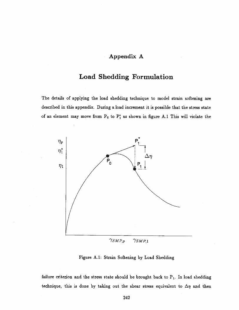
Appendix A
Load Shedding Formulation
The details of applying the load shedding technique to model strain softening are
described in this appendix. During a load increment it is possible that the stress state
of an element may move from P0 to P as shown in figure A.1 This will violate the
Figure A.1: Strain Softening by Load Shedding
failure criterion and the stress state should be brought back to P1. In load shedding
technique, this is done by taking out the shear stress equivalent to and then
‘r/p
*
1i
P1
1
7SMP,p 7SMP,i
242

Appendix A. Load Shedding Formulation 243
transferring it to the adjacent stiffer elements. The detailed steps of this procedure
will be as follow:
1. Estimate the stress ratio (n’, Figure A.1) in the strain softening region corre
sponding to the shear strain (7sMp,1) using equation 3.63 as
7i 1r + (i— a,,) exp { — K (ysMP, 1 — 7SMP,p
) } (A. 1)
2. Estimate the amount of stress ratio that has to be taken out as
(A.2)
3. Evaluate the changes in the Cartesian stress vector {/.o-}Ls which corresponds
to
4. Evaluate the force vector {/.F}Ls equivalent to {/.o}Ls.
5. Take out {Lo-}Ls from the failed element and set its moduli to low values.
6. Carry out a load step analysis with {F}Ls as the incremental load vector.
7. Check whether any other elements violate the failure criteria and undergo soft
ening, and if so, repeat the load shedding procedure.
A.1 Estimation of {zSJ}Ls
In order to estimate the changes in the Cartesian stress vector, it is easier to first
estimate the changes in principal stresses. By differentiating equation 3.34 in terms
of principal stresses the following equation can be obtained:
T
1213 + 1113(02 + £73) —1112(U2U3) Lo
18I1213+1113(U3+Ui)1112(U3U1) U2 (A.3)
‘213 +1113(ui + £72) —1112(U1t72)
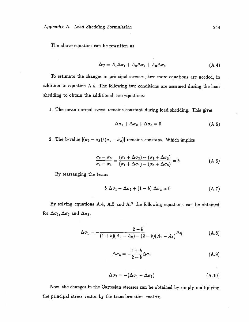
Appendix A. Load Shedding Formulation 244
The above equation can be rewritten as
A1/o-1 + A2Io2H- A3z3 (A.4)
To estimate the changes in principal stresses, two more equations are needed, in
addition to equation A.4. The following two conditions are assumed during the load
shedding to obtain the additional two equations:
1. The mean normal stress remains constant during load shedding. This gives
1 + + Lo3 0 (A.5)
2. The b-value [(02 — 03)/(01 — 03)] remains constant. Which implies
(A6)Oi — 03 — (o- + Zoi) — (03 + Lo3) —
By rearranging the terms
(A.7)
By solving equations A.4, A.5 and A.7 the following equations can be obtained
for 02 and o3:
2—b
H- b)(A3 — A2) —(2— b)(A1 — A2)(A.8)
1+b(A.9)
—(Lri + 3) (A.l0)
Now, the changes in the Cartesian stresses can be obtained by simply multiplying
the principal stress vector by the transformation matrix.
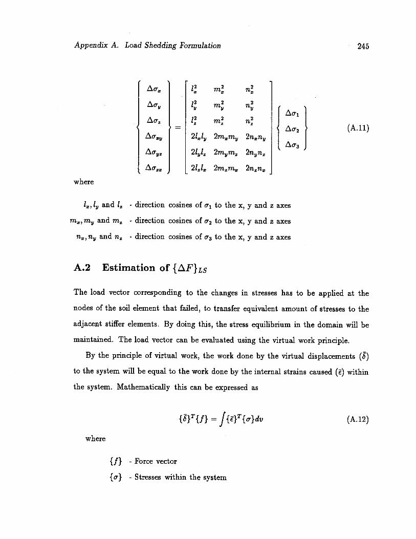
Appendix A. Load Shedding Formulation 245
l m
12 m2 n2y
12 m2(A.11)
2ll, 2mm 2n,nIO3
2l,l 2mm2 2nn
2mm 2nzna,
where
1a li,, and l - direction cosines of o to the x, y and z axes
m, m and m - direction cosines of O2 to the x, y and z axes
n, n and n - direction cosines of 03 to the x, y and z axes
A.2 Estimation of {F}Ls
The load vector corresponding to the changes in stresses has to be applied at the
nodes of the soil element that failed, to transfer equivalent amount of stresses to the
adjacent stiffer elements. By doing this, the stress equilibrium in the domain will be
maintained. The load vector can be evaluated using the virtual work principle.
By the principle of virtual work, the work done by the virtual displacements (8)
to the system will be equal to the work done by the internal strains caused () within
the system. Mathematically this can be expressed as
{}T{f} = J{}Tfr}dv (A.12)
where
{ f} - Force vector
{o} - Stresses within the system
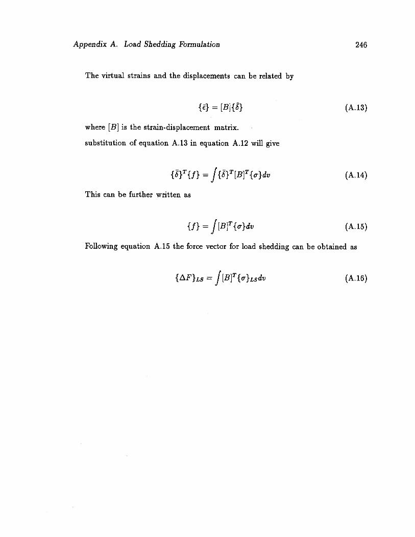
Appendix A. Load Shedding Formulation 246
The virtual strains and the displacements can be related by
{} = [B]{} (A.13)
where [B] is the strain-displacement matrix.
substitution of equation A.13 in equation A.12 will give
{}T{f} = J{}T[B]T{}dv (A.14)
This can be further written as
{f} = J[B]Tfr}dv (A.15)
Following equation A.15 the force vector for load shedding can be obtained as
{IF}Ls J[B]T{U}LSdV (A.16)

Appendix B
Relative Permeabilities and Viscosities
Some detailed explanations which are needed in the evaluation of equivalent per
meability are given in this appendix. To evaluate the equivalent permeability, the
relative permeability and the viscosity values of the pore fluid components are nec
essary. The first section explains how to calculate the relative permeabilities and the
equivalent permeability through an example data set. The viscosity values of water
at different temperatures are given in section 2. Section 3 gives some insights into
the viscosity of hydrocarbon gases and how to evaluate it.
B.1 Calculations of relative permeabilit ies
B.1.1 Relevant equations
The relative permeabilities of water, gas and oil can be obtained from the following
equations:
Jc° S1k° S_qrog 9’ row w a a— Jo
1 t-’w JgI
krw = — A2)A3 (B.2)
krow B1(B2 — Sw)B3 (B.3)
krg = C1(S9 — (B.4)
247
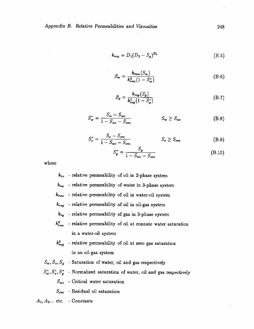
Appendix B. Relative Permeabilities and Viscosities 248
k,.09 = D1(D2 —S9)D3 (B.5)
— krow(Sw)B6/3W
— k0(1 — S,,)
— k,.09(S9)9ko (1—S (
r09\ 9
= 5;— Swc
S S (B.8)Wc om
s S0— Sorn
So > Som (B.9)wc om
9‘9i c’ C’‘-‘uc ‘-‘Orn
where
k,.0 - relative permeability of oil in 3-phase system
k,. - relative permeability of water in 3-phase system
- relative permeability of oil in water-oil system
- relative permeability of oil in oil-gas system
krg - relative permeability of gas in 3-phase system
k - relative permeability of oil at connate water saturation
in a water-oil system
k09 - relative permeability of oil at zero gas saturation
in an oil-gas system
S,,, S, S - Saturation of water, oil and gas respectively
S, S, 5 - Normalized saturation of water, oil and gas respectively
- Critical water saturation
5om - Residual oil saturation
A1,A2... etc. - Constants

Appendix B. Relative Permeabilities and Viscosities 249
= 0.2
k° —107’OW
= 1.0
A1 = 1.820
B1 = 2.769
C1 = 2.201
= 1.640
A2 = 0.20
B2 = 0.80
C2 = 0.05
D2 = 0.80
A3 = 2.375
B3 = 1.996
C3 = 2.704
= 2.547
= 0.5
I-sw = 8 x 10⁴Pa.s
k = 1 x 10²m2
S, 0.4
= 2OPa.s
Sg = 0.1
= 2 x 10⁵Pa.s (at 30°C)
B.1.3 Sample calculations
By substituting the data into the relevant equations
0.5 — 0.2=0.5
1 — 0.2 — 0.2
0.15;
= 1 — 0.2 — 0.2= 0.1667
0.4— 0.2= = 0.3333
1 — 0.2 — 0.2
The equivalent permeability is given by
kEQ=kI-o P’g
B.1.2 Example data
(B.11)
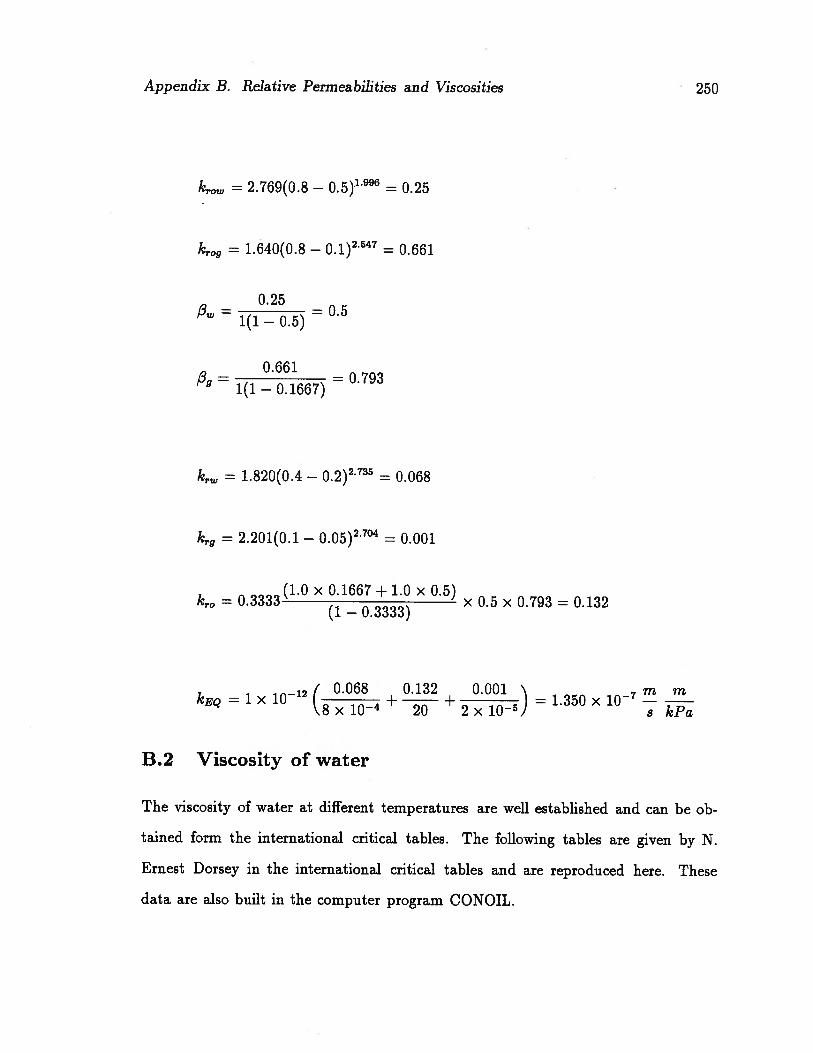
Appendix B. Relative Permeabilities and Viscosities 250
= 2.769(0.8 — 0.5)1.996 = 0.25
krog = 1.640(0.8 0.1)2.547 = 0.661
0.25= 1(1 — 0.5)
= 0.5
0.6610 793
— 1(1 — 0.1667) —
krw 1.820(0.4 — 0.2)2.735 = 0.068
k,.9 = 2.201(0.1 — 0.05)2.704 = 0.001
k,.0 = 0.3333(1.0 X 0.1667+1.0 X 0.5)
X 0.5 X 0.793 = 0.132
—12 / 0.068 0.132 0.001‘ m m
kEQ = 1 >< 108 x 10
+20
+2 x 10⁵)
1.350 x 10 —
B.2 Viscosity of water
The viscosity of water at different temperatures are well established and can be ob
tained form the international critical tables. The following tables are given by N.
Ernest Dorsey in the international critical tables and are reproduced here. These
data are also built in the computer program CONOIL.

Appendix B. Relative Permeabiiities and Viscosities
Table B.1: Viscosity of water between 0 and 1000 C
251
Values in rnillipoises (1, 12, 16, 17, 22, 24, 30, 31, 32, 38)
C 0 1 2 3 4 5 6 7 8 9
0 17.93* 17.326 16.74* 16.19a 15.67. 15.18* 14.72* 14.28* 13.872 13.47,10 13.097 12.73s. 12.39o 12.06i 11.748 11.44? 11.15* 10.875 10.60s 10.34o20 10.087 9.843 9.60* 9.38* 9.16i 8.94. 8.74* 8.55i 8.368 8.181
30 8.004 7.834 7.67* 7.511 7.35 7.20* 7.064 6.92 6.791 6.66140 6.536 6.41s 6.29* 6.184 6.075 5.97* 5.86* 5.77* 5.67s 5.58250 5.492 5.40s 5.32* 5.236 5.153 3.07s 4.99* 4.918 4.84a 4.77o60 4.69* 4.62s 4.56i 4.495 4,43i 4.36* 4.30* 4.24s 4.186 4.12s
70 4.07i 4.01* 3.96z 3.909 3.8.5? 3.806 3.756 3.70* 3,66i 3.61s80 3.57. 3.52* 3.483 3.44. 3.39* 3.35i 3.31? 3.27* 3.24* 3.20390 3.16* 3.13* 3.095 3.061 3.027 2.994 2.96a 2.93* 2.89. 2.86*
100 2.83* 2.82 2.79 i 2.76 2.73 2.70 2.67 2.64 2.62 2.59
At a pressure ox 1 atm., = a/(b + t)”.
At a pressure of P kg/cm2, ,7p = ?7i[l + k,(P — 1) X 10’J.‘11 is the value , when P is 1 kg/cm2,which may be taken asThe unit of , is the poise unless otherwise stated.
Table B.2: Viscosity of water below 00 C
H,O ov 100°C (16)
Values as recorded by author accord with I. C. T. values below100°C; the others are given as he has published them. Thepressure is that of the saturated vapor at the temperaturesindicated.
4, °C 110 120 130 140 150 1601000,7 2.56 2.32 2.12 1.96 1.84 1.74
Table B.3: Viscosity of water above 1000 C
H20 BELOW 0°C (39)
Values corrected and adjusted to accord with I. C. T. valuesabove 0°C
FoR,.1Ux.E AND UNITS
the value of,7 at 1 atm.
—2 —4 —5 —6 —8 —10100077 19.1 20.5 21.4 22.2 24.0 26.0
Appendix B. Relative Permeabilities and Viscosities 252
B.3 Viscosity of hydrocarbon gases (from Carr et al., 1954)
The viscosity of hydrocarbon gases can be expressed as a function of reduced pressures
and temperatures, i.e.,
(B.12)IL1
where
- viscosity of gas at reduced temperature TR
and at reduced pressure FR
pi - viscosity of gas at atmospheric pressure and given temperature
TR - temperature/critical temperature (in absolute units)
PR - pressure/critical pressure (in absolute units)
If the gas is a mixture of hydrocarbons, the pseudo-critical concept has to be
applied. Thus, in place of critical temperature and critical pressure, the pseudo-
critical temperature and pressure have to be used. The pseudo-critical temperature
is given by
(B.13)
The pseudo-critical pressure is given by
PPc=XzFci (B.14)
where
- mol fraction of component i in the mixture
- critical temperature of component i in absolute units
- critical pressure of component i in absolute units
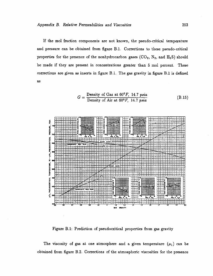
a)‘—
4-
)d
0.4
,4
U)
.•-
40
-c
•c:
a)a)—
l
_
a)U)
a)U)
‘—I
;0
to0o
—-d
-c
if)
0a)
Cl)U
)C
)c
;4-
.4
0-4-a
ca)
U)
0Q)
-4to
a)Cl)
)-U
)to
cdto
toa)
o0
--
O-
_-
Cl)H
0-4
a);-1
p-
‘da)
to-0
to
:-
EQ0
a)
4‘-
-4
a)0
-dl-
4a)
0-
a)E
.a
a)0
‘0
Cl)
V
0U
)a,
.4)
;-4a
‘.
0a)4
.44
a)U
)U
)U
)a)
-a)
.-I
_4
--4
-4-a‘-4
(3+
l-40
I—’
-4-4
4)‘-4
2a)
,.D0
:a)
a)a)0-
.a)
-4
--
c3
0
toCl)
r0
oa)
Cl)-4
Cl)a)
0a)
-4
..
.—a)
to-
0Cl)
‘-4
0-d
:0a)
o-0
Cl)d
U)
-4
l-40o00
0
U)
0
:111
if)
-I
:j:==iiI111JW
i1L111FW1
IMIII:.4a.3wvo, an,.!J.L
IiL
IJ_L
LL
_
Ian3L,
tTITFITIITII
—
Ii
IiI1IM1ll1ll12t:
tll1llllillllhIt
r-.l,6A•woIi,,_,
ltav
d’
“llD
c1llllt
4.q_4‘....
,s,wou,,.uo,;i.
Cl)-
II
IIIIc!:
1
U)
VISd
‘UflS
SW
dV
OI1
W3O
OflS
d,d
d—
U.
‘311fl1VU
3dY131
VO
4J4l4OO
OflS
did
Ia,

‘-4.,
oCD
CDCD
.
2U
)
‘-i’
CDCD
,- CD-$
-+
:-
CDo
CD
CD0
.q-
), (
—.
- CDI—
0‘d
c-
I—.
CD
j.
p,U
)0
CD0
0—
.+
0U
)0 p
CD
•-•
CD
pU
)CD
p;;.
U)
o op
0‘—
4.,
U)
,-4.
,
4,_
-’o
o9’
09’
9,
•-
CD,-
,CD
CDCD
‘‘
CDU
)
0•
•P
‘-d
0o
‘-UCD
•C
D9’
4-4—]0
_..
,,.
rJ ‘-U “l
CD0
CD4-
sU
)-
I-s
CD-
r pCD
CDCD
CD—
..
U)
9’:-‘
‘-s
CDU
)CD
C’)
+p
CDCD
--
b0
1E
LJ
P0
‘-UU
)CD 1
4-s 9’
‘-5
4--
CD—
.—
‘0 9, —.‘ .
I—-
4-s CD
C’)
U)
9’
‘-5 CD •
CDo
0 9, 0 -“ CD 0
U)
‘)
oo
4--
U) 0 o 0 4-+
) ,- _4-4 - 0 CD oq
- ‘-UO
u,
9’CD 0
CD
‘-5 CD U) 0 0 U)
‘-4-
0 4-f
,
‘-1 0 0 p I-s 0 9, U) CD ci) 9, 0 CD 9’ 0 U)
‘-U CD ‘-5 CD
0 0 0 ‘-4-
CD U) 0 4-f
,
‘-5 0 0 9, I-s 0 0 CD 9, CD 0 CD U) CD ‘-5
‘-4-
‘-U 0 ‘-4-
U)
O’3
‘-5 CD
VIS
CO
SIT
Y,
AT
IATM
.•AJ, CENTI
PO
IS
8°
80
öb
0b
ION
AD
OE
D-i-
1-ii
F1t4
-iI—
tWttW
ttIt
lilt
I1I
8
FL*J1
i1ir
4’i
‘-U >1 9, ‘-4-
‘-U I..
II+
H+
FfA
ii(r
LjtI
U11
M1W
411
1FF
PII1I
IlIFF
1Fvr1
I14-4a
I4JYL
4AY1
4n’i1
fFIl
CU
UII
ttt1
IIIi
1iV
IlI1
IJ11tI
fl1V
IIIA
FII
,I1
VIl
LIt
IUI
rV
111)
14-I
11
11
11
71
11
5I
1111
1Il
ILU
I.i
ii.n
rrii
iD
IAl
rU1
Er[
I4fl
EC
s.P
111)
11It
’ll
il/l
iV
IKJ
y‘i
iC
OA
CC
TIO
uD
OE
OD
1l1
(—19
ItlA
1-I
II
IA-t
-f-
To
,sc
—G
Pt.
,8
CO
RII
CC
1IO
NA
DO
LDT
I)V
ISC
—G
14
-1 0
r
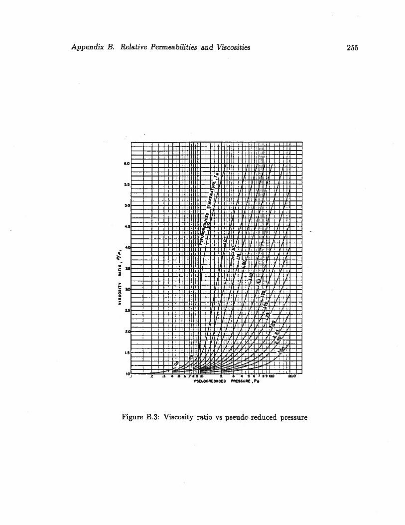
Appendix B. Relative Permeabilities and Viscosities 255
J )‘‘ =
.-‘. .L. I. .iL. - -
— IH
-- -- —
- .LL.... -- — -
III,
£1 / ‘
:iL.-(-L — -
.k L .t.1- -r ‘--j-•-p.j-r / I—— —--
•- -ir-rr ,4t—— —-- -. 1—-
—— ---r ,
1 “i:0 —. — — I - H- 1! -f-J4 —
1.. — — — -- , -rv i- r;- — -
: ia:: .±Ik— — —- - ‘4- I
1”E
-
___
i!::: .
I ,.,.‘77 I.— - — . .-f ‘ T
—— - - -- r/r7 7 -i,.’_.
_____
i --- :..4 -
__
— . . — -
IC
____
— . —--—-- — — L I . —
2 3 4 .5 6 7.6LD 2 3 4 56 7I9
PSEUCOREDUGED PRESSURC
Figure B.3: Viscosity ratio vs pseudo-reduced pressure
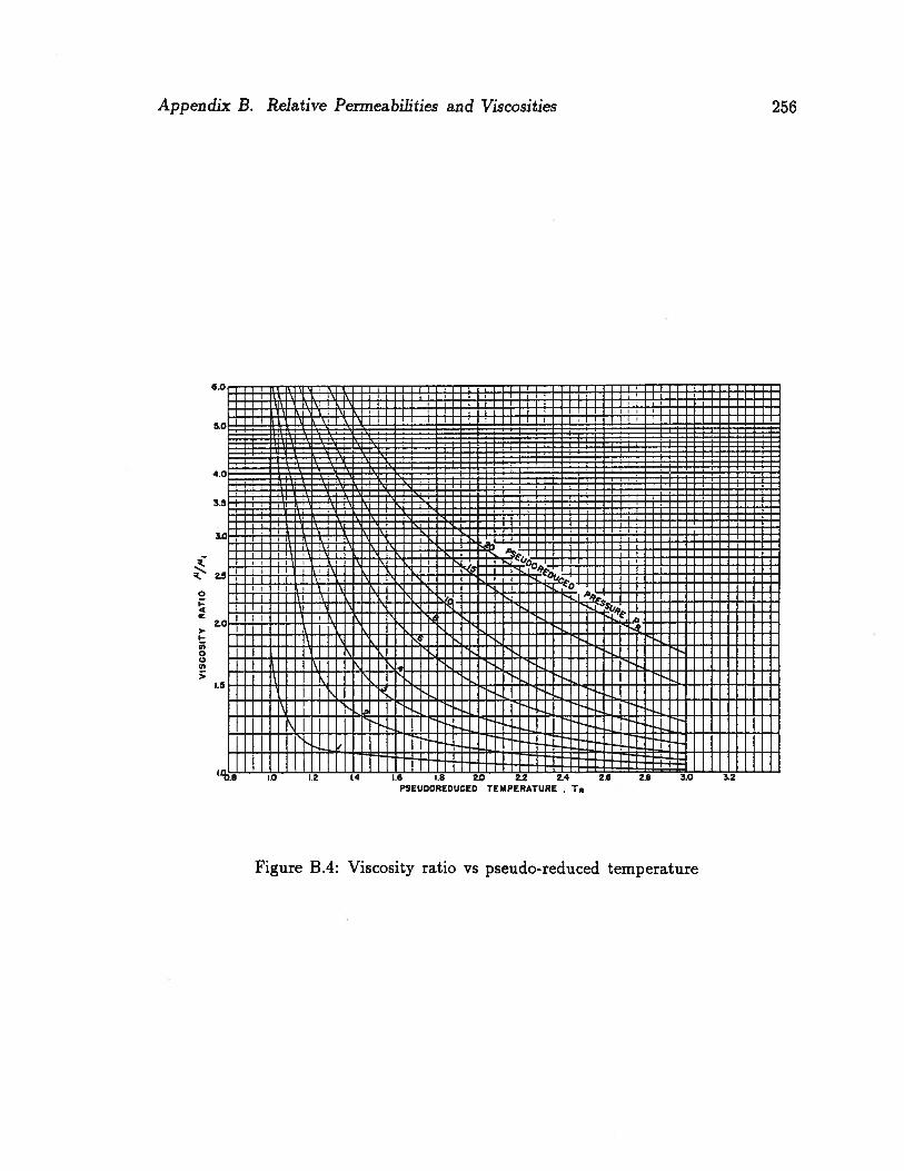
VIS
CO
SIT
YR
AT
IO01
gU
I
__
_
-.---I
H111
HTTD
11I
—-
--
--
--
--
-Iil
lII
lili
liP
I::
E::
:tft
11
1It
t1U
ftI
tumiH
t—
——
—-—- -
AI
III
IIL
iII
IU—
ti±
fliI
JJ-J
kH
lfl-
Ct)—
II
II
i—i-
-i-r
nI
II
IIi
-i-H
I]II
UH
i]CD
—————
-—--
11—
i—1
11
1r
ru1
x4
-rrr
rlL
I-1
-rrt
Trl
]r—
—,——-—-
—- -‘1
I-I
44
II
FL
I+
1H
I-I-
li-I
’1I
III-I
I-I4
J4— ——
1111]J
i—rL
uII
Il-i
-rU
JJJ±
LuII
UL
--—
J-t.I
-[T
u-1-
T[I
TIT
FF
IFrI
TI
1LW
IU
—T
II
III
1—H
ilII
H-I-
flU-
CDi4
———
- -—
IIIT
Iii4
-nT
rLi4
-rn
1-r
Tr
-:
--:
LIJ}
tT[I
WIT
WIT
h[IL
-1J[I-
±tf1±1
±H±ft
H1±th
_:_L
::,
iii[1
4r1±
1±th
tinlll
:I
—-
itiI
lF{*
fl+}1
+HI1
{If
,,
i:
---
rtri
uwiw
rmirr
ni—
L——
—--- -
414-
U4
1414
-I-IW
-1411
1III-
C
3::
::
:•
4I111
II1Ht-1[
1-
I:
7:
::
:41
WhI
I-fll-
UIL[
N-
‘-
EE
HE
E
Appendix B. Relative Permeabilitics and Viscosities 257
temperature was 195°F, and the test pressure was 1800 psig (1815 psia). The gravity
of the liberated gas was determined by the use of tared glass weighing balloon. The
gas gravity was found to be 0.70 18 (air = 1.0). The calculation of viscosity will be as
follows:
1. Molecular weight 0.7018 x 28.95 20.31
2. For which:
Pseudo-critical pressure 667 (figure B.1)
Pseudo-critical temperature = 390 (figure B.1)
If the mole fractions of the hydrocarbon components are known the above values
can be calculated using equations B.13 and B.14.
3. From figure B.2:
Viscosity at one atmosphere () = 0.01223cp
4. Pseudo-reduced pressure = 1, 815/667 = 2.721
Pseudo-reduced temperature = (460 + 195)/390 = 1.679
5. From figures B.3 and B.4:
IL/IL1 = 1.28
6. Therefore,
The viscosity at 1800 psig and 195°F = 1.28 x 0.01223 = 0.01565cp

Appendix C
Subroutines in the Finite Element Codes
C.1 2-Dimensional Code CONOIL-Il
The 2-dimensional code has been divided into two separate programs; the ‘Geometry
Program’ and the ‘Main Program’. The main reason for having as two separate
programs is to reduce the effort on the user. The geometry program automatically
generates and numbers the midside and interior nodes. It also renumbers the elements
and nodes to minimize the front width and creates a input file for the main program,
containing the relevant information about the finite element mesh. The main program
does the analysis. The geometry program for the 2-dimensional version consists of
11 subroutines and the main program consists of 58 subroutines. The details of the
subroutines are described herein.
C.1.1 Geometry Program
The subroutines in the geometry program and their functions are as follow:
ADDS - forms element-node links.
BCONI - sets up element constants.
FFIN - reads free format input.
MAKENZ - generates an array which contains the number of degrees of freedom
associated with each node.
MIDPOR - generates mid-side pore pressure nodes.
MIDSID - generates mid-side displacement nodes.
258

Appendix C. Subroutines in the Finite Element Codes 259
MLAPZ - marks last appearances of nodes by making them negative.
OPTEL - optimizes and renumbers the elements for frontal solution.
RDELN - reads line data.
SFWZ - calculates the front width for symmetric solution.
SORT2 - changes the element numbers to conform with new ordering.
C.1.2 Main Program
The subroutines in the main program and their functions are given below.
BCON - calculates element constants.
CHANGE - removes/adds elements from geometry mesh and calculates implied
loading.
CHECK - scrutinizes the input data to main program.
CHKLST - checks if there are any changes in fixity for the load increment.
COMP - computes the pore fluid compressibility and permeability.
DATM - reads material property data.
DETJCB - calculates the determinant of the Jacobian matrix.
DHYPER - calculates the stress-strain matrix for elastic model.
DILATE - computes the volume change due to shear deformation (used with hyper
bolic model).
DISTLD - calculates equivalent nodal loads.
DSYMAL - finds the principal stresses and their directions (contains 5 subroutines;
TRED3, TRBAK3, TQLRAT, TQL2, DTRED4).
ELMCH - scrutinizes the list of elements.
EQLBM - calculates unbalanced nodal loads.
EQLIB - calculates nodal forces balancing element stresses.
ERR - records and lists data errors.
FFIN - reads free format input.
Appendix C. Subroutines in the Finite Element Codes 260
FFLOW - calculates amount of flow and updates saturations.
FIXX - updates list of nodal fixities.
FLOWST - calculates vectors for coupled consolidation analysis.
FORMB - forms ‘B’(shape function derivative) matrix.
FRONTZ - frontal solution routine for symmetric matrix.
GETEQN - gets the coefficients of the eliminated equations.
INSIT - sets up in-situ stresses and the equivalent nodal forces.
INSTRS - prints the in-situ stresses before first increment.
INV - inverts a matrix.
LSHED - carries out load shedding operation.
LSTIFA - calculates the element stiffness matrix using fast stiffness formation.
LSTIFF - calculates the element stiffness matrix for elastic model.
MAKENZ - generates an array which contains the number of degrees of freedom
associated with each node.
MBOUND - rearranges the boundary conditions in terms of degrees of freedom.
MLAPZ - marks last appearances of nodes by making them negative.
MODULI - calculates moduli of the soil elements for elastic model.
MSUB - main controlling routine.
PLAS - calculates the stress-strain matrix for elasto-plastic model.
PRINC - calculates principal stresses.
RDN - reads specified range in 1-dimensional array.
REACT - calculates the reactive forces on restrained boundaries.
SCAN - checks for any changes in fixities.
SELF - calculates self weight loads.
SELl - computes nodal forces equivalent to self weight loads.
SFR1 - calculates shape functions and derivatives for 1-dimensional integration along
element edges.
Appendix C. Subroutines in the Finite Element Codes 261
SFWZ - estimates the front width for symmetric matrix solution.
SHAPE - calculates shape functions and derivatives.
SOFT * calculates the overstress for strain softening.
STIF - calculates element stiffness matrix for elasto-plastic model.
STOREQ - writes the terms in a buffer zone when an array becomes saturated.
TEMP - calculates the equivalent force vector terms due to temperature changes.
UFRONT - frontal solution routine for unsymmetric matrix.
UPARAL - allocates storage for subroutine UPOUT.
UPOUT - updates and prints the results.
VISG - calculates viscosity of gas.
VISO - calculates viscosity of oil.
VISW - calculates viscosity of water.
WRTN - writes a specified range in a 1-dimensional array.
ZERO1 - initializes 1-dimensional array.
ZERO2 - initializes 2-dimensional array.
ZERO3 - initializes 3-dimensional array.
ZEROI1 - initializes 1-dimensional integer array.
C.2 3-dimensional code CONOIL-Ill
The 3-dimensional code has been developed based on the same sequence of procedures
as the 2-dimensional code. It consists of 43 subroutines and the details of those are
given below.
BOUND - expands the nodal fixity data in terms of degree of freedom.
CHANGE - removes/adds elements from geometry mesh and calculates implied
loading.
COMP - computes the pore fluid compressibility and permeability.
DMAT - reads material property data.
Appendix C. Sn bron tines in the Finite Element Codes 262
DRIVER - main controlling routine.
EPM - calculates stress-strain matrix for elasto-plastic model.
EQLIB - calculates nodal forces balancing element stresses.
FFLOW - calculates amount of flow and updates saturations.
FIXX - updates list of nodal fixities.
FLSD - calculates load vector for load shedding.
FTEMP - calculates force vector terms due to temperature changes.
GETEQN - gets the coefficients of the eliminated equations.
HYPER - calculate moduli values for hyperbolic model.
INSIT - sets up in-situ stresses and the equivalent nodal forces.
JACO - evaluates Jacobian matrix, its determinant and inverse.
LAYOUT - reads nodal geometry data and stores in relevant arrays.
LFIX - sets the load vector for fixed boundaries.
LOAD - evaluates the load vector for applied loads.
LSHED - routine to perform load shedding.
MAKESF - finds last appearance of the nodes, frontwidth and the destination vector.
MFLOW - updates saturations and flow at mid-step.
MINV - inverts a matrix
PRIN - finds the principal stresses and their directions (contains 5 subroutines;
TRED3, TRBAK3, TQLRAT, TQL2, DTRED4).
PRNOUT - calculates, updates and prints the results.
RDN - reads specified range in 1-dimensional array.
SBMATX - calculates B’(shape function derivative) matrix.
SELF - calculates self weight loads.
SELl - calculates self weight loads for gravity changes.
SFRONT - frontal solution routine for symmetric matrix.
SHAPE - calculates shape functions and its derivatives.
Appendix C. Subroutines in the Finite Element Codes 263
SHAPE2 - calculates shape functions and derivatives for 2-dimensional integration.
SMDF - sets up arrays giving nodal degrees of freedom and the first degree of freedom
of the nodes.
STIFF - calculates element stiffness matrix.
STOREQ - writes the terms in a buffer zone when an array becomes saturated.
STRL - calculates and updates stress level.
TEMP - calculates nodal temperature changes.
UFRONT - frontal solution routine for unsymmetric matrix.
UPDATE - updates the results at mid-step for second iteration.
VISG - calculates viscosity of gas.
VISO - calculates viscosity of oil.
VISW - calculates viscosity of water.
WRTN - writes a specified range in a 1-dimensional array.
ZERO 1 - initializes 1-dimensional array.
ZERO2 - initializes 2-dimensional array.
ZERO3 - initializes 3-dimensional array.
ZEROI1 - initializes 1-dimensional integer array.
ZEROI2 - initializes 2-dimensional integer array.
Appendix D
Amounts of Flow of Different Phases
The formulation for the multi-phase flow presented in chapter 5 considers an equiv
alent conductivity term to model the effects of the different phases in the pore fluid.
This does not give the individual amounts of flow of the fluid phase components.
However, at any time, these individual amounts of flow can be easily estimated by
knowing the total amount of flow, and the relative permeabilities and viscosities of
the phase components. The details of this calculation are presented in this appendix.
To illustrate the steps involved the example problem given in chapter 7 is considered
here.
In the oil sand layer the zone from where the fluid flow occurs, can be obtained from
the temperature contour plot or the pore pressure contour plot (refer to figures 7.17
and 7.18). Such a zone for the example problem is shown in figure D.1.
The fluid flow zone can be divided into a number of zones of different effective mobil
ities. Here, the flow zone is divided into three (zones A, B and C in figure D.1) and
the effective mobilities of the fluid phase components are assumed constant within a
zone. The grater the number of zones the better the results will be.
The mobility of a fluid phase component ‘1’ can be written as
kmikkri
(D.1)
where
kmi - mobility of phase 1
k - intrinsic permeability of the sand matrix (m2)
264
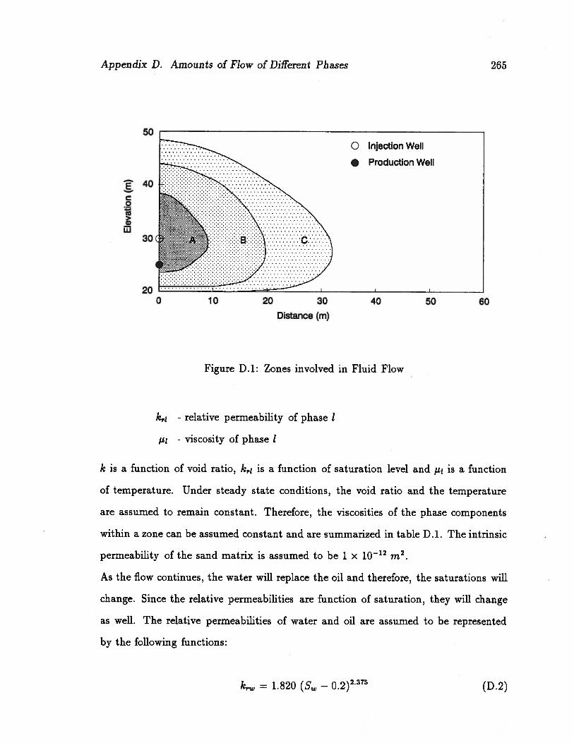
Appendix D. Amounts of Flow of Different Phases 265
50
0 Injection Well
• Production Well
E 40
40 0 60
Distance (m)
Figure D .1: Zones involved in Fluid Flow
k,.1 - relative permeability of phase I
IL1 - viscosity of phase 1
k is a function of void ratio, k,.1 is a function of saturation level and 1u is a function
of temperature. Under steady state conditions, the void ratio and the temperature
are assumed to remain constant. Therefore, the viscosities of the phase components
within a zone can be assumed constant and are summarized in table D.l. The intrinsic
permeability of the sand matrix is assumed to be 1 x 10¹² m2.
As the flow continues, the water will replace the oil and therefore, the saturations will
change. Since the relative permeabilities are function of saturation, they will change
as well. The relative permeabilities of water and oil are assumed to be represented
by the following functions:
= 1.820 (S — 0.2)2.375 (D.2)

Appendix D. Amounts of Flow of Different Phases 266
Table D.1: Average Viscosities and Temperatures in Different Zones
Zone Area (m2) ii(mPa.s) u0(mPa.s) Temp. (°C)
A 96 0.20 8 220
B 252 0.48 40 140
C 312 0.65 1000 50
k,.0 = 2.769 (0.8— S)’996 (D.3)
Now, let us assume that the total flow of water and oil for a time interval /t be
LVT. This total amount of flow will comprise the water and oil flow in all three zones
considered. The effective mobility of water considering all three zones can be given
as,= (kmw)A aA + (kmw)B aB + (kmw) ac
(D.4)aA + a + ac
Where, aA, aB and ac are the areas of zones A, B and C respectively. Similarly, the
effective mobility of oil considering all three zones can be given as,
— (kmo)A aA + (kmo)B aB + (kmo) acmo aA + aB + ac
Then, the amounts of water and oil flow in the total flow can be estimated as,
A TI TI mwL.Vw VT ke j i.e
mw
= LVT e e (D.7)mw mo
Now, because of the flow of oil from the oil sand layer, saturations will change and
those should be updated at the end of the time step. To calculate the new saturations,
the amounts of flow in individual zones should be estimated. This can be done as
follows.

Appendix D. Amounts of Flow of Different Phases 267
For example, the amount of water flow from zone A can be given by,
fAT? AT? mw A aAiI_1Vw)A = LVw
(kmw)A aA + (kmw)B aJ3 + (kmw) ac
Similarly, all the individual amounts of flow of water and oil in different zones can be
calculated.
Assume that the saturation of oil in zone A at the beginning of a time step be (S0).
Then, the saturation of water in zone A at the beginning of the time step will be,
(S) = 1 — (S0) (D.9)
The volume of oil in zone A at the beginning of the time step will be given by,
(V0) = aA n (S0) (D.1O)
The amount of oil flow from zone A will be,
IAT?\ AT? mo A aAL.1Vo)A =
(kmo)A aA + (kmo)B aB + (kmo) ac
Then, the volume of oil in zone A at the end of the time step will be,
(V (V0) — (V0)A (D.12)
and the new oil saturation will be,
(S0)(V0)
(D.13)fl aA
The new saturation of water in zone A will be given by,
(S) = 1 — (S0) (D.14)
Likewise, the saturations in all the zones can be updated. Then, by knowing the new
saturations, the relative permeabilities of the phase components can be estimated and
subsequently, the new amounts of water and oil flow can be calculated. These steps

Appendix D. Amounts of Flow of Different Phases 268
of calculations can be continued with time in a step by step manner until the flow of
oil ceases or the amount of oil flow becomes insignificant.
The above described procedure is applied to the example problem considered here.
The initial saturation and the mobilities of water and oil in different zones are given
in table D.2.
Table D.2: Initial Saturations and Mobilities of Water and Oil
Zone Sw S kmw(108m/s) kmo(108m/s)
A 0.3 0.7 37.6 85.1
B 0.3 0.7 19.8 17.0
C 0.3 0.7 11.6 0.68
The stepwise calculations for the amounts of flow and saturations of water and oil
are tabulated in table D.3. The saturations and the mobilities of water and oil at the
end of time t = 300 days, are given in table D.4, which can be compared with table
D.2.

Appendix D. Amounts of Flow of Different Phases 269
Table D.3: Calculation of Flow and Saturations with Time
Time (S)A (S)B (S)c (S0)A (S0)B (S0)c iW0(days) (m3/day) (m3/day)
0 0.300 0.300 0.300 0.700 0.700 0.700 2.54 2.642 0.394 0.319 0.301 0.606 0.681 0.699 3.89 1.294 0.435 0.330 0.301 0.565 0.670 0.699 4.29 0.896 0.461 0.339 0.302 0.539 0.661 0.698 4.49 0.698 0.479 0.346 0.302 0.521 0.654 0.698 4.61 0.5710 0.494 0.352 0.302 0.506 0.648 0.698 4.69 0.4915 0.525 0.365 0.303 0.475 0.635 0.697 4.82 0.3620 0.546 0.375 0.303 0.454 0.625 0.697 4.89 0.2925 0.562 0.384 0.304 0.438 0.616 0.696 4.94 0.2430 0.574 0.392 0.304 0.426 0.608 0.696 4.97 0.2140 0.595 0.405 0.305 0.405 0.595 0.695 5.01 0.1750 0.610 0.417 0.306 0.390 0.583 0.694 5.04 0.1460 0.622 0.426 0.307 0.378 0.574 0.693 5.06 0.1270 0.632 0.435 0.307 0.368 0.565 0.693 5.07 0.1180 0.640 0.443 0.308 0.360 0.557 0.692 5.08 0.1090 0.647 0.450 0.308 0.353 0.550 0.692 5.09 0.09100 0.653 0.456 0.309 0.347 0.544 0.691 5.10 0.08125 0.667 0.471 0.310 0.333 0.529 0.690 5.11 0.07150 0.678 0.484 0.311 0.322 0.516 0.689 5.12 0.06175 0.686 0.495 0.312 0.314 0.505 0.688 5.13 0.05200 0.693 0.505 0.313 0.307 0.495 0.687 5.13 0.05250 0.704 0.522 0.315 0.296 0.478 0.685 5.14 0.04300 0.713 0.536 0.317 0.287 0.464 0.683 5.15 0.03
Table D.4: Saturations and Mobilities of Water and Oil after 300 Days
Zone S S kmw(108m/s) kmo(108m/s)
A 0.71 0.29 1826 2.61
B 0.54 0.46 352 4.75
C 0.32 0.68 16.7 0.64
Appendix E
User Manual for CONOIL-Il
E.1 Introduction
CONOIL-Il is a finite element program for consolidation analysis in oil sands under
plane strain and axisymmetric conditions. The program includes an elasto-plastic
stress strain model and a formulation to analyze multi-phase fluid flow. It also con
siders temperature effects on stresses and fluid flow in the analysis.
The program can be used to carry out transient, drained or undrained analysis us
ing the same material data base. Elements can be removed to simulate excavation.
Provisions exist for specifying various boundary conditions such as pressure, force,
displacement and pore pressure. Though the program is particularly suited for prob
lems in oil sands, it can be applied for a range of geotechnical problems such as dam
and heavy foundation analyses.
The intention of this manual is to provide sufficient information for an analyst with
a strong geotechnical background to be able to prepare an input file and run the
program. Detailed explanations such as analytical formulation, method of analysis,
formation of stiffness matrix, solving routines etc. can be found in Srithar (1993).
CONOIL-Il has been divided into two separate programs: the ‘Geometry Program’
and the ‘Main Program’. The main purpose of this split is to reduce the effort on the
user. The geometry program automatically generates and numbers the mid-side and
interior nodes. It also renumbers the elements and nodes to minimize the front width
and creates an input file for the main program, containing the relevant information
about the finite element mesh. Therefore, the Geometry Program has to be run first
270
Appendix E. User Manual for CONOIL-Il 271
and the link file has to be submitted to the Main Program.
The data for both the Geometry Program and the Main Program is free format
i.e, particular data items must appear in the correct order on a data record but
they are not restricted to appear only between certain column positions. The data
items are indicated below by mnemonic names, i.e., names which suggest the data
item required by the program. The FORTRAN naming convention is used: names
beginning with the letters I, J, K, L, M and N show that the program is expecting an
INTEGER data item whereas names beginning with any other letter show that the
program is expecting a REAL data item. The only exception is the material property
data where the actual parameter notations are retained to avoid confusions. All the
material property data are real. INTEGER data items must not contain a decimal
point but REAL data items may optionally do so. REAL data items may be entered
in the FORTRAN exponent format if desired. Individual data items must not contain
spaces and are separated from each other by at least one space. Detailed explanations
for some of the records are given in section E.4.
Comments may be included in the input data file in exactly the same way as for the
FORTRAN program. Any line that has the character C in column 1 is ignored by the
programs. This facility enables the user to store information relating to values, units
assumed etc. permanently with the input data rater than separately. The program
only read data from the first 80 columns of each line.
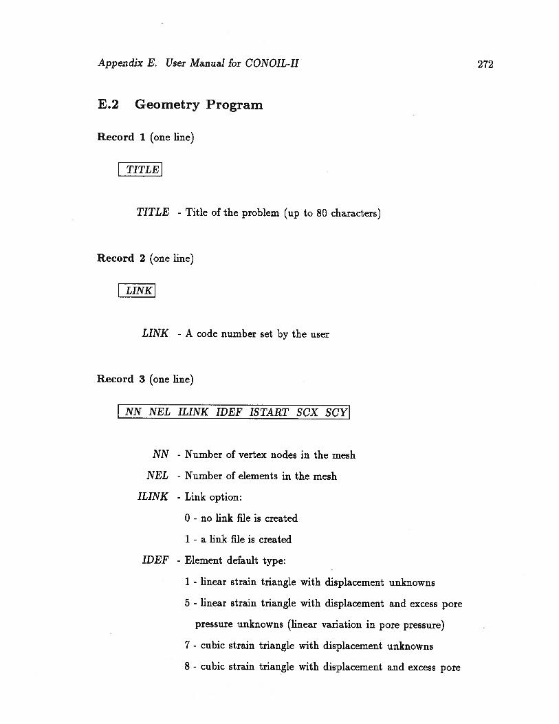
Appendix E. User Manual for CONOIL-Il 272
E.2 Geometry Program
Record 1 (one line)
TITLE
TITLE - Title of the problem (up to 80 characters)
Record 2 (one line)
I LINK
LINK - A code number set by the user
Record 3 (one line)
NN NEL ILINK IDEF ISTART SCX SCY
NN - Number of vertex nodes in the mesh
NEL - Number of elements in the mesh
ILINK - Link option:
0 - no link file is created
1 - a link file is created
IDEF - Element default type:
1 - linear strain triangle with displacement unknowns
5 - linear strain triangle with displacement and excess pore
pressure unknowns (linear variation in pore pressure)
7 - cubic strain triangle with displacement unknowns
8 - cubic strain triangle with displacement and excess pore
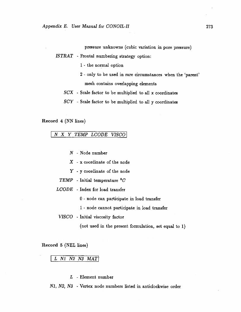
Appendix E. User Manual for CONOIL-Il 273
pressure unknowns (cubic variation in pore pressure)
ISTRAT - Frontal numbering strategy option:
1 - the normal option
2 - only to be used in rare circumstances when the parent’
mesh contains overlapping elements
SCX - Scale factor to be multiplied to all x coordinates
SCY - Scale factor to be multiplied to all y coordinates
Record 4 (NN lines)
N X Y TEMP LCODE VISCO]
N - Node number
X - x coordinate of the node
Y-
y coordinate of the node
TEMP - Initial temperature °C
LCODE - Index for load transfer
o - node can participate in load transfer
1 - node cannot participate in load transfer
VISCO - Initial viscosity factor
(not used in the present formulation, set equal to 1)
Record 5 (NEL lines)
ILN1N2N3MATI
L - Element number
Ni, N2, N3 - Vertex node numbers listed in anticlockwise order

Appendix E. User Manual for CONOIL-Il 274
MAT - Material zone, number in range 1 to 10

Appendix E. User Manual for CONOIL-Il 275
E.3 Main Program
Record. 1 (one line)
TITLEI
TITLE - Title of the problem (up to 80 characters)
Record 2 (one line)
I LINKI
LINK - Code number set by the user
Record 3 (one line)
I NPLAX NMAT INCJ INC2 IPPJM IUPD ICOR ISELFI
NPLAX - Plane strain/Axisymmetric analysis option:
0 - plane strain
1 - axisymmetric
NMAT - Number of material zones
INC1 - Increment number at start of analysis
INC2 - Increment number at finish of analysis
IPRIM - Number of elements to be removed to from primary mesh
IUPD - Element default type:
1 - linear strain triangle with displacement unknowns
5 - linear strain triangle with displacement and excess pore
pressure unknowns (linear variation in pore pressure)

Appendix E. User Manual for CONOIL-Il 276
7 - cubic strain triangle with displacement unknowns
8 - cubic strain triangle with displacement and excess pore
pressure unknowns (cubic variation in pore pressure)
ISTRAT - Frontal numbering strategy option:
1 - the normal option
2 - only to be used in rare circumstances when the ‘parent’
mesh contains overlapping elements
SCX - Scale factor to be multiplied to all x coordinates
SOY - Scale factor to be multiplied to all y coordinates
Record 4 (One line only)
MXITER DIOONV PATM
MXITER - Maximum number of iterations per increment for dilation
and load transfer purposes (zero defaults to 5)
DICONV - Convergence criterion for change in force vector from
dilation calculations (zero defaults to 0.05)
PATM - Atmospheric pressure in user’s units (SI: 101.3 kPa;
Imperial 2116.2 psf (zero defaults to 101.3 kPa)
Record 5 (for HYPERBOLIC stress-strain model)
(Records 5.1 to 5.10 have to repeated NMAT times.
Records 5.5 to 5.10 are necessary only if IMPF = 2.
Records 5.1 to 5.4 are given separately for HYPERBOLIC and ELASTO-PLASTIC
stress-strain models )

Appendix E. User Manual for OONOIL-II 277
Record 5.1
MAT IMODEL e KE n Rf KB m DUO k k
MAT - Material property number. All elements given the same
number in the Geometry Program have the following properties
IMODEL - Stress-strain model number. Use C7 for Hyperbolic model
e - Initial void ratio
KE - Elastic modulus constant
n - Elastic modulus exponent
Rf - Failure ratio
KB - Bulk modulus constant
m - Bulk modulus exponent
DUO - Determines whether Drained/Undrained/Consolidation analysis
i) DUO = 0.0 Drained analysis
ii) DUO = B1 (liquid bulk modulus) - Undrained analysis
NOTE: B1 in the range of 100 to 500 B5k (soil bulk modulus) is
equivalent to using a Poisson’s ratio of 0.495 to 0.499.
If there are temperature changes, use consolidation routine
to do undrained analysis.
iii) DUO = 7i (unit weight of liquid) - Consolidation analysis
- total unit weight of soil
- permeability in x direction
- permeability in y direction
Record 5.2
c - v ot q’cv - B B0

Appendix E. User Manual for CONOIL-Il 278
c - Cohesion
- Friction angle at a confining pressure of 1 atmosphere
L4 - Reduction in friction angle for a ten fold increase in
confining pressure—
- 0 (No parameter at present)
- Constant dilation angle. To be specified if the dilation
option is used.
a8t - Coefficient of temperature induced structural reorienta
tion. Only used in temperature analysis.
- Constant volume friction angle. Only used with dilation
option.—
- 0 (No parameter at present)
B - Bulk modulus of the water
B0 - Bulk modulus of the oil
Record 5.3
/J’30,0 ‘H H -\U U S S1 cw a0
1’3o,o - Viscosity of oil at 300 C and 1 atmosphere (in Pa.s)
(used in three phase flow, built-in oil viscosity correlation)
- Function to modify Henry’s constant for temperature
H=H+)H*IXT
H - Henry’s coefficient of solubility
- Function to modify bubble pressure for temperature
U - Bubble pressure (Oil/Gas saturation pressure)
S - Initial degree of saturation varying between 0 and 1. (S
= 1 implies 100% saturation)

Appendix E. User Manual for CONOIL-Il 279
Sf - Saturation at which fluid begins to move freely. (Used
for modifying permeability. 1 is generally close to zero)
- Coefficient of linear thermal expansion of water
cx0 - Coefficient of linear thermal expansion of oil
- Coefficient of linear thermal expansion of solids
Record 5.4
ISIGE 151GB IMPF IDILAT ILSHD I
ISIGE - Option to calculate Young’s modulus
o - use mean normal stress
1 - use minor principal stress
ISIGB - Option to calculate bulk modulus
o - use mean normal stress
1 - use minor principal stress
IMPF - Multi phase flow option
o - fully saturated
1 - partially saturated
2 - three phase fluid flow (needs additional parameters)
IDILAT - Dilation option
o - No dilation
1 - Use constant dilation angle
2 - Use Rowe’s stress-dilatancy theory
ILSHD - Load transfer option
o - do not perform load transfer
1 - perform load transfer by keeping o constant
2 - perform load transfer by keeping On constant

Appendix E. User Manual for CONOIL-Il 280
Record 5 (for ELASTO-PLASTIC stress-strain model)
(Records 5.1 to 5.10 have to repeated NMAT times.
Records 5.5 to 5.10 are necessary only if IMPF = 2.
Records 5.1 to 5.4 are given separately for HYPERBOLIC and ELASTO-PLASTIC
stress-strain models )
Record 5.1
MAT IMODEL e KE n (R1) KB m DUO k %
MAT - Material property number. All elements given the same
number in the Geometry Program have the following properties
IMODEL - Stress-strain model number
= 5 Cone type yielding only (single hardening)
= 6 Cone and Cap type yielding (double hardening)
e - Initial void ratio
KE - Elastic modulus constant
n - Elastic modulus exponent
(Rf) - Failure ratio in the hardening rule (cone yield)
KB - Bulk modulus constant
m - Bulk modulus exponent
DUO - Determines whether Drained/Undrained/Consolidation analysis
i) DUO = 0.0 Drained analysis
ii) DUO = B1 (liquid bulk modulus) - Undrained analysis
NOTE: B1 in the range of 100 to 500 B8,, (soil bulk modulus) is
equivalent to using a Poisson’s ratio of 0.495 to 0.499.
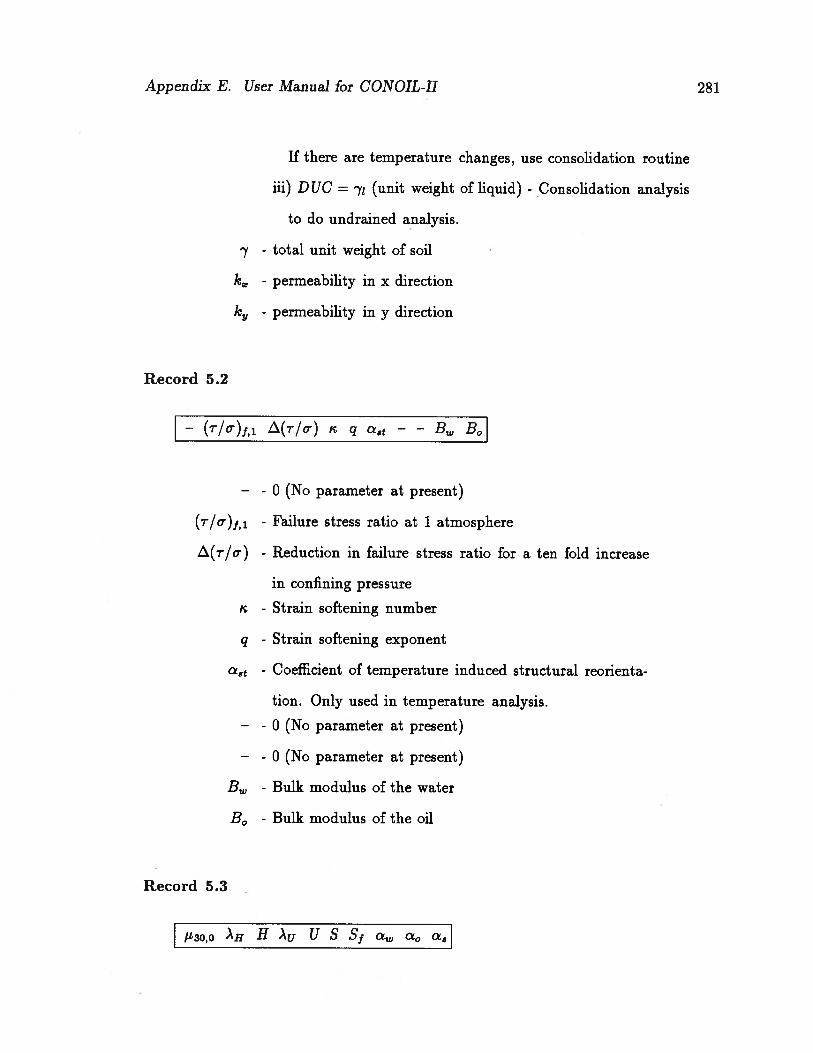
Appendix E. User Manual for CONOIL-Il 281
If there are temperature changes, use consolidation routine
iii) DUO = 71 (unit weight of liquid) - Consolidation analysis
to do undrained analysis.
- total unit weight of soil
- permeability in x direction
k - permeability in y direction
Record 5.2
(r/o)1,i (r/o-) q — — B B0
—
- 0 (No parameter at present)
(T/o-)f,i - Failure stress ratio at 1 atmosphere
(r/o) - Reduction in failure stress ratio for a ten fold increase
in confining pressure
- Strain softening number
q - Strain softening exponent
a8t - Coefficient of temperature induced structural reorienta
tion. Only used in temperature analysis.—
- 0 (No parameter at present)
—
- 0 (No parameter at present)
B - Bulk modulus of the water
B0 - Bulk modulus of the oil
Record 5.3
f-3O,O H H u U S S a a0
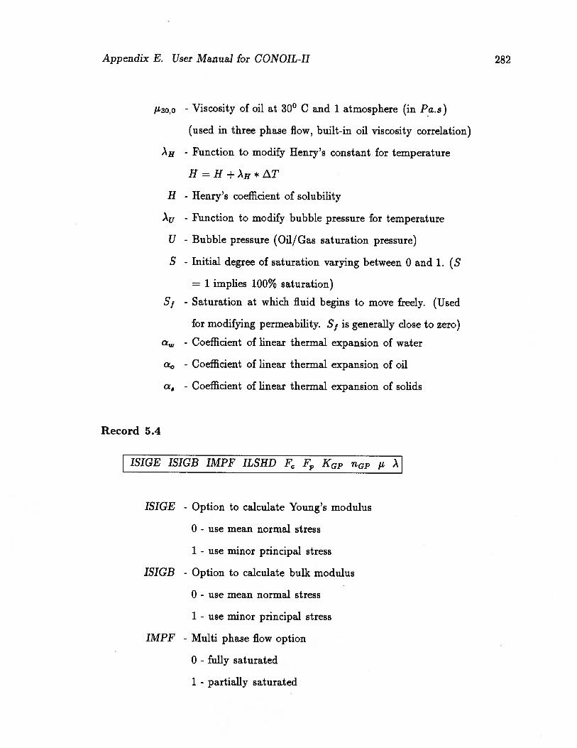
Appendix K User Manual for CONOIL-Il 282
1130,0 - Viscosity of oil at 300 C and 1 atmosphere (in Pa.s)
(used in three phase flow, built-in oil viscosity correlation)
- Function to modify Henry’s constant for temperature
H =H+\H*T
H - Henry’s coefficient of solubility
- Function to modify bubble pressure for temperature
U - Bubble pressure (Oil/Gas saturation pressure)
S - Initial degree of saturation varying between 0 and 1. (S
= 1 implies 100% saturation)
S, - Saturation at which fluid begins to move freely. (Used
for modifying permeability. S is generally close to zero)
- Coefficient of linear thermal expansion of water
- Coefficient of linear thermal expansion of oil
a5 - Coefficient of linear thermal expansion of solids
Record 5.4
ISIGE ISIGB IMPF ILSHD F F KGp GP 11
ISIGE - Option to calculate Young’s modulus
0 - use mean normal stress
1 - use minor principal stress
ISIGB - Option to calculate bulk modulus
0 - use mean normal stress
1 - use minor principal stress
IMPF - Multi phase flow option
0 - fully saturated
1 - partially saturated

Appendix E. User Manual for GONOIL-Il 283
2 - three phase fluid flow (needs additional parameters)
ILSHD - Load transfer option
0 - do not perform load transfer
1 - perform load transfer by keeping o constant
2 - perform load transfer by keeping o constant
- Collapse modulus number (cap yield)
F - Collapse modulus exponent (cap yield)
KGp - Plastic shear parameter (cone yield, hardening rule)
GP - Plastic shear exponent (cone yield, hardening rule)
- Flow rule intercept (cone yield)
- Flow rule slope (cone yield)
Record 5.5 (necessary only if IMPF = 2, all are real variables except IV)
Sw So Sg S S k0g IVL, IVO IV9
S - Initial water saturation
S, - Initial oil saturation
S9 - Initial gas saturation
(S + S0 + S must be equal to 1)
5om - Residual oil saturation
S - Connate water saturation (irreducible water saturation)
- Relative permeability of oil at connate water saturation
(oil-water)
- Relative permeability of oil at zero gas saturation (oil-gas)
IV, - Options to estimate viscosity of water
0 - use a given constant value (in Pa.s)
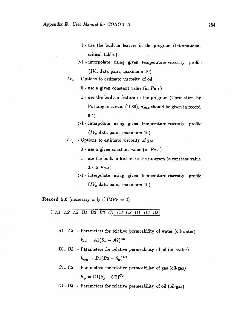
Appendix E. User Manual for CONOIL-Il 284
1 - use the built-in feature in the program (International
critical tables)
>1 - interpolate using given temperature-viscosity profile
(IV data pairs, maximum 10)
IV, - Options to estimate viscosity of oil
0 - use a given constant value (in Pa.s)
1 - use the built-in feature in the program (Correlation by
Puttangunta et.al (1988), to,o should be given in record
6.4)
>1 - interpolate using given temperature-viscosity profile
(1V0 data pairs, maximum 10)
IVg - Options to estimate viscosity of gas
0 - use a given constant value (in Pa.s)
1 - use the built-in feature in the program (a constant value
2.E-5 Pa.s)
>1 - interpolate using given temperature-viscosity profile
(I17 data pairs, maximum 10)
Record 5.6 (necessary only if IMPF = 2)
Al A2 A3 Bi B2 B3 Cl C2 03 Dl D2 D3
Al...A3 - Parameters for relative permeability of water (oil-water)
krw = A1(S — A2)A3
Bl...B3 - Parameters for relative permeability of oil (oil-water)
= B1(B2 — S)B3
Cl... 03 - Parameters for relative permeability of gas (oil-gas)
k,.9 = C1(S9 — C2)c3
Dl...D3 - Parameters for relative permeability of oil (oil-gas)

Appendix E. User Manual for CONOIL-Il 285
k,.09 = D1(D2
Record 5.7 (necessary only if IMPF = 2)
I Fl F2 F31
Fi...F3 - Parameters for oil-gas capillary pressure
of gas (oil-gas)
Pc = Fl Pa(S9 — F2)’3
Record 5.8 (necessary only if IMPF = 2 and IV,,, = 0 or >1)
V,,, (ifIV=0)
Vi Ti V2 T2•.• I (if IV, , 1, IV, data pairs, maximum 10)
V - Constant viscosity value of water (in Pa.s)
Vi,... - Viscosity values in the given profile (in Pa.s)
Ti,... - Temperature values in the given profile (in °C)
Record 5.9 (necessary only if IMPF = 2 and 1V0 = 0 or >1)
V01 (ifIV0=0)
Vi Ti V2 T2•.. I (if 1V0> 1, 1V0 data pairs, maximum 10)
V0 - Constant viscosity value of oil (in Pa.s)
Vi,... - Viscosity values in the given profile (in Pa.s)
Ti,... - Temperature values in the given profile (in °C)
Record 5.10 (necessary only if IMPF = 2 and 1V9 = 0 or >1)

Appendix E. User Manual for CONOIL-Il 286
(ifIV=0)
I Vi Ti V2 T2... I (if IVg> 1, 1V9 data pairs, maximum 10)
- Constant viscosity value of gas (in Pa.s)
Vi,... - Viscosity values in the given profile (in Pa.s)
Ti,... - Temperature values in the given profile (in °C)
Record 6 ((IPRIM-1)/10 + 1 lines, only if IPRIM> 0)
I Li L2
Li,... - List of element numbers to be removed to form mesh at
the beginning of the analysis (LPPJM element numbers)
There must be 10 data per line, except the last line
Record 7 (one line only)
INSIT NNI NELl NO UT I
INSIT - In-situ stress option:
0 - Set in-situ stresses to zero
1 - Direct specification of in-situ stresses
NNI - Number of nodes in-situ mesh
NELl - Number of elements in-situ mesh
NOUT - In-situ stress printing option:
0 - Do not print the in-situ stresses
1 - Print the variables at the centroids of each element
2 - Print the variables at each integration point per element
and print the equilibrium loads for in-situ stresses.
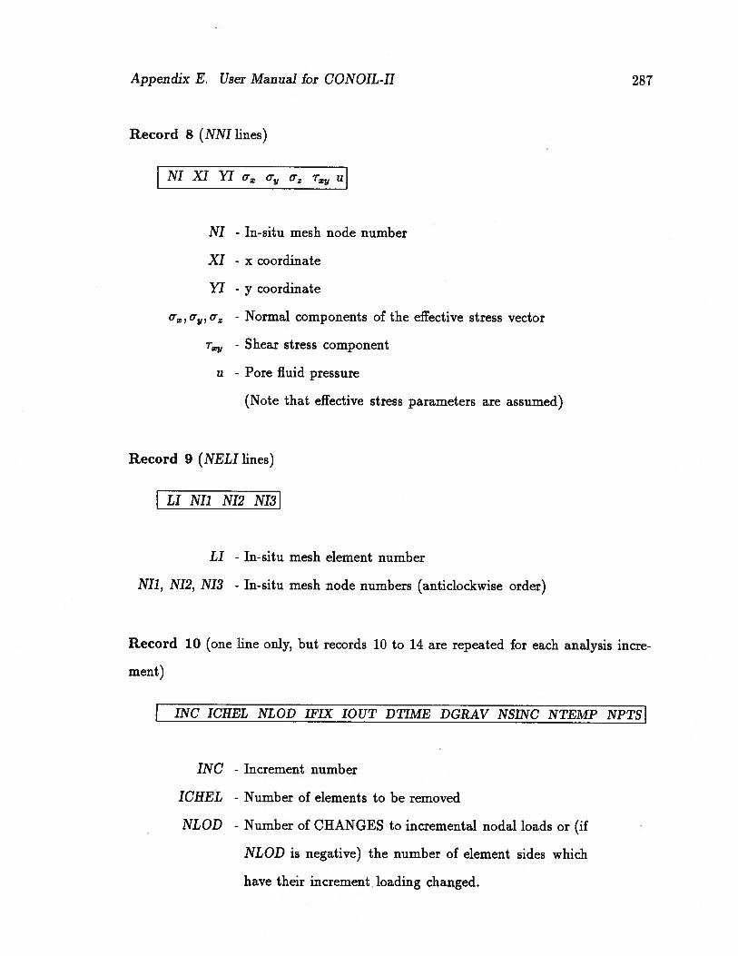
Appendix E. User Manual for CONOIL-Il 287
Record 8 (NNI lines)
NI XI Yl o- o, o- r u
NI - In-situ mesh node number
XI - x coordinate
Y1-
y coordinate
o, o, o - Normal components of the effective stress vector
- Shear stress component
ii - Pore fluid pressure
(Note that effective stress parameters are assumed)
Record 9 (NELl lines)
LI NIl N12 NI3]
LI - In-situ mesh element number
NIl, N12, N13 - In-situ mesh node numbers (anticlockwise order)
Record 10 (one line only, but records 10 to 14 are repeated for each analysis incre
ment)
INC ICHEL NLOD IFIX lOUT DTIME DGRAV NSINC NTEMP NPTSI
INC - Increment number
ICHEL - Number of elements to be removed
NLOD - Number of CHANGES to incremental nodal loads or (if
NLOD is negative) the number of element sides which
have their increment loading changed.

Appendix E. User Manual for CONOIL-Il 288
IFIX - Number of changes to nodal fixities
lOUT - Output option for this increment - a four digit number
abcd where:a - out of balance loads and reactions
o - no out of balance loads
1 - out of balance loads at vertex nodes
2 - out of balance loads at all nodes
b - option for prescribed boundary conditions (e.g. fixity
condition or equivalent nodal loads at specified nodes)
o no information printed
I - data printed for each relevant d.o.f
c - option for general stresses
o - no stresses printed
1 - stresses at element centroids
2 - stresses at integration points
d - option for nodal displacements
o - no displacements printed
1 - displacements at vertex nodes
2 - displacements at all nodes
DTIME - Time increment for consolidation analysis
DGRAV - Increment in gravity level
(change in number of gravities)
NSINC - The number of sub increments (this is presently equal to 1)
NTEMP - Number of changes to nodal temperature
DGRAV - Number of data pairs in the temperature-time history profile
Record 11 ((ICHEL-1)/1O + 1 lines, only if ICHEL > 0)
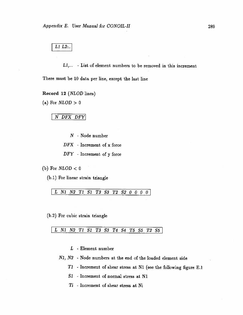
Appendix E. User Manual for CONOIL-Il 289
rLi
Li,... - List of element numbers to be removed in this increment
There must be 10 data per line, except the last line
Record 12 (NLOD lines)
(a) For .1\TLOD > 0
NDFX DFY1
N - Node number
DFX - Increment of x force
DFY - Increment of y force
For NLOD < 0
(b.1) For linear strain triangle
LNJN2TJS1 T3S3T2S200001
(b.2) For cubic strain triangle
I L Ni N2 Ti Si T3 S3 T4 S4 T5 55 T2 S
L - Element number
Ni, N2 - Node numbers at the end of the loaded element side
Ti - Increment of shear stress at Ni (see the following figure E.1
Si - Increment of normal stress at Ni
Ti - Increment of shear stress at Ni
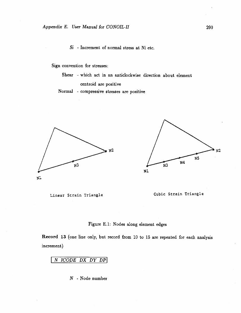
Appendix E. User Manual for CONOIL-Il 290
Si - Increment of normal stress at Ni etc.
Sign convention for stresses:
Shear - which act in an anticlockwise direction about element
centroid are positive
Normal - compressive stresses are positive
Ni
N2
Linear Strain Triangle Cubic Strain Triangle
Figure E.1: Nodes along element edges
Record 13 (one line only, but record from 10 to 15 are repeated for each analysis
increment)
N ICODE DX DY DPI
NSN4
N - Node number

Appendix E. User Manual for CONOIL-Il 291
ICODE - A three digit code abc which specifies the degrees of
freedom associated with this node that are fixed to par
ticular valuesa - fix for x direction
o - node is free in x direction
1 - node is to have a prescribed incremental displacement
DXb - fix for y direction
o - node is free in y direction
1 - node is to have a prescribed incremental displacement
DYc - fix for excess pore pressure
o - no prescribed excess pore pressure
1 - the increment of excess pore pressure at this node is to
have a prescribed value DP
2 - the absolute excess pore pressure at this node is to have
a zero value for this and all subsequent increments of
analysis
DX - Prescribed displacement in x direction
DY - Prescribed displacement in y direction
DP - Prescribed pore pressure
Record 14 (NTEMP lines, only if NTEMP > 0)
N TEM1 TIMEJ TEM2 TIME2 .J (NPTS data pairs, maximum 15)
N - Node number
TEMJ,... - Temperature in the given temperature time profile
TIMEJ,... - Time in the temperature time profile

Appendix E. User Manual for CONOIL-Il 292
E.4 Detail Explanations
Detailed explanations for some of the records are given in this section to provide a
better understanding.
E.4.1 Geometry Program
Record 2
The geometry program stores basic information describing the finite element mesh on
a computer disk file (the ‘Link’ file) which is subsequently read by the Main Program.
A user of CONOIL will often set up several (different) finite element meshes and run
the Main Program several times for each of these meshes. In order to ensure that a
particular Main Program run accesses the correct Link file the LINK number is stored
on the Link file by the Geometry program and must be quoted correctly in the input
for the Main Program. Hence LINK should be set to a different integer number for
each finite element mesh that the user specifies.
Record 3
LDEF (Element Types)
The element type is defined by LDEF which at present can take one of four values
associated with the elements shown in Figure E.2. The variation of displacements
(and consequently strains) and where appropriate, the excess pore pressures are sum
marized in table E.1. All elements are basically standard displacement finite elements
which are described in most texts on the finite element method.
Although CONOIL allows the user complete freedom in the choice of element type,
the following recommendations should lead to the selection of an appropriate element
type:
(i) Plane Strain Analysis
For drained or undrained analysis use element type 1 (LST) and for consolidation
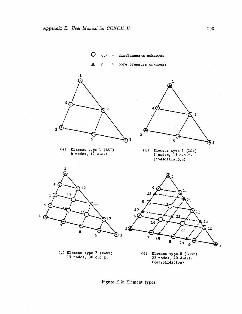
Appendix E. User Manual for CONOIL-Il 293
0 u,v — displacement unknowrs
A p — pore pressure unknowns
a.1.
6
22
S2
(a) Element type 1 (LST) (b) Element type 5 (LST)6 nodes, 12 d.o.f. 6 nodes, 15 d.o.f.
(consolidation)
412
—._. 1216
216 11
- / ,‘ 112
/ 106
/ 1//
102S - /
.188 19 9 1
(c) Element type 7 (CuST) (d) Element type 8 (CuST)15 nodes, 30 d.o.f. 22 nodes, 40 d.o.f.
(consolidation)
Figure E.2: Element types
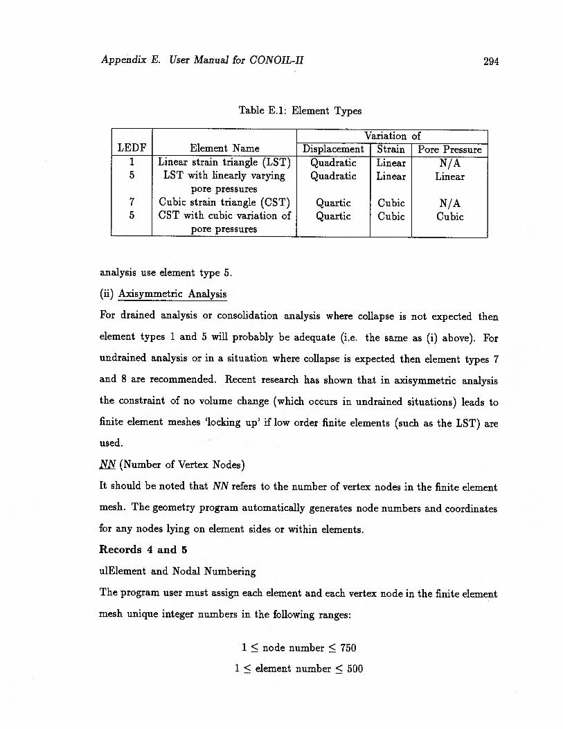
Appendix E. User Manual for CONOIL-Il 294
Table E.1: Element Types
Variation ofLEDF Element Name Displacement Strain Pore Pressure
1 Linear strain triangle (LST) Quadratic Linear N/A5 LST with linearly varying Quadratic Linear Linear
pore pressures7 Cubic strain triangle (CST) Quartic Cubic N/A5 CST with cubic variation of Quartic Cubic Cubic
pore_pressures
analysis use element type 5.
(ii) Axisymmetric Analysis
For drained analysis or consolidation analysis where collapse is not expected then
element types 1 and 5 will probably be adequate (i.e. the same as (i) above). For
undrained analysis or in a situation where collapse is expected then element types 7
and 8 are recommended. Recent research has shown that in axisymmetric analysis
the constraint of no volume change (which occurs in undrained situations) leads to
finite element meshes ‘locking up’ if low order finite elements (such as the LST) are
used.
NN (Number of Vertex Nodes)
It should be noted that NN refers to the number of vertex nodes in the finite element
mesh. The geometry program automatically generates node numbers and coordinates
for any nodes lying on element sides or within elements.
Records 4 and 5
ulElement and Nodal Numbering
The program user must assign each element and each vertex node in the finite element
mesh unique integer numbers in the following ranges:
1 < node number 750
1 < element number < 500

Appendix E. User Manual for CONOIL-Il 295
It is not necessary for either the node numbers or the element numbers to form
a complete set of consecutive integers, i.e., there may be ‘gaps’ in the numbering
scheme adopted. This facility means that users may modify existing finite element
meshes by removing elements without the need for renumbering the whole mesh. The
Geometry Program assigns numbers in the range 751 upwards to nodes on element
sides and in element interiors.
MAT Material Zone Numbers
The user must assign a zone number (in the range 1 to 10) to each finite element.
The zone number associates each element with a particular set of material properties
(Record 5 of Main Program input). Thus, if there are three zones of soil with different
material properties, they can be modelled by different stress-strain relations. (Note:
the material zone numbers have to consecutive).
E.4.2 Main Program
Record 2
The link number must be the same as that specified in the Geometry Program input
data for the appropriate finite element mesh (see Record 2 in section E.4.1).
Record 3
NPLAX Plane strain/Axisymmetric
The selection of axes and the strain conditions under plane strain and axisymmetric
conditions are shown in figures E.3 and E.4 respectively.
NMAT Number of Materials
sl NMAT must be equal to the number of different material zones specified in the
geometry program.
IPRIM
CONOIL allows excavations to be modelled in an analysis via the removal of elements
as the analysis proceeds. All the elements that appear at any stage in the analysis
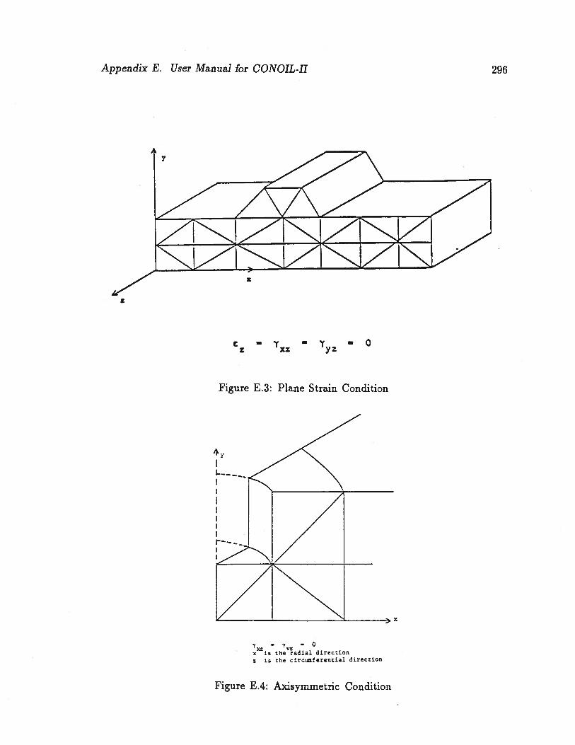
Appendix E. User Manual for CONOIL-Il 296
KZZ.
Figure E.3: Plane Strain Condition
xis the’adia1 direcSon
z is the circwnferentiai direction
Figure E.4: Axisymmetric Condition

Appendix E. User Manual for CONOIL-Il 297
must have been included in the input data for the Geometry Program. IPRIM is the
number of finite elements that must be removed to form the initial (or primary) finite
element mesh before the analysis is started.
IUPD
IUPD = 0: This corresponds to the normal assumption that is made in linear elas
tic finite element programs and also in most finite element programs with nonlinear
material behaviour. External loads and internal stresses are assumed to be in equi
librium in relation to the original (i.e., undeformed) geometry of the finite element
mesh. This is usually known as the ‘small displacement’ assumption.
IUPD = 1: When this option is used the nodal coordinates are updated after each
increment of the analysis by adding the displacements undergone by the nodes during
the increment to the coordinates. The stiffness matrix of the continuum is then
calculated with respect to these new coordinates during the next analysis increment.
The intension of this process is that at the end of the analysis equilibrium will be
satisfied in the final (deformed) configuration. Although this approach would seem to
be intuitively more appropriate when there are significant deformations it should be
noted that it does not constitute a rigorous treatment of the large strain/displacement
behaviour for which new definitions of strains and stresses are required. Various
research workers have examined the influence of a large strain formulation on the load
deformation response calculated by the finite element method using elastic perfectly
plastic models of soil behaviour. The general conclusion seems to be that the influence
of large strain effects is not very significant for the range of material parameters
associated with most soils. In most situations, the inclusion of large strain effects
leads to a stiffer load deformation response near failure and some enhancement of
the load carrying capacity of the soil. If a program user is mainly interested in the
estimation of a collapse load using an elastic perfectly plastic soil model then it is
probably best to use the small displacement approach (i.e., sl IUPD = 0). Collapse

Appendix E. User Manual for CONOIL-Il 298
loads can then be compared (and should correspond) with those obtained from a
classical theory of plasticity approach.
ISELF
In many analyses the stresses included in the soil by earth’s gravity will be insignificant
compared to the stresses induced by boundary loads (e.g., in a laboratory triaxial
test). For this type of analysis it is convenient to set ISELF = 0 and correspondingly
7 set to zero in Record 5.
When the stresses due to the self weight of the soil do have a significant effect in
the analysis then ISELF should be set to 1 and 7should be set to the appropriate
(non zero) value. If the program simulates an excavation by removing elements then
the assumption is made that the original in-situ stresses were in equilibrium with the
various densities (-y) in the Records 5.
Records 7, 8 and 9
In the nonlinear analyses performed by CONOIL, the stiffness matrix of a finite el
ement is dependent on the stress state within the element. In general, the stress
state will vary across an element and the stiffness terms are calculated by integrat
ing expressions dependent on these varying stresses over the volume of each element.
CONOIL integrates these expressions numerically by ‘sampling’ the stresses at par
ticular points within the element and then using standard numerical integration rules
for triangular areas.
The purpose of Records 7, 8 and 9 is to enable the program to calculate the stresses
before the analysis starts. Although the in-situ mesh elements are specified in exactly
the same way as finite elements in the Geometry Program input, it should be noted
that they are not finite elements. The specification of the ‘in-situ mesh’ is simply a
device to allow stresses to be calculated at all integration points by a process of linear
interpolation over triangular regions. Thus, if the initial stresses vary linearly over
the finite element mesh, it is usually possible to use an in-situ mesh with one or two
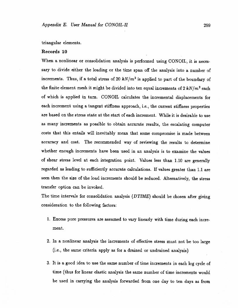
Appendix E. User Manual for CONOIL-Il 299
triangular elements.
Records 10
When a nonlinear or consolidation analysis is performed using CONOIL, it is neces
sary to divide either the loading or the time span off the analysis into a number of
increments. Thus, if a total stress of 20 kN/m2 is applied to part of the boundary of
the finite element mesh it might be divided into ten equal increments of 2 kN/m2 each
of which is applied in turn. CONOIL calculates the incremental displacements for
each increment using a tangent stiffness approach, i.e., the current stiffness properties
are based on the stress state at the start of each increment. While it is desirable to use
as many increments as possible to obtain accurate results, the escalating computer
costs that this entails will inevitably mean that some compromise is made between
accuracy and cost. The recommended way of reviewing the results to determine
whether enough increments have been used in an analysis is to examine the values
of shear stress level at each integration point. \Talues less than 1.10 are generally
regarded as leading to sufficiently accurate calculations. If values greater than 1.1 are
seen then the size of the load increments should be reduced. Alternatively, the stress
transfer option can be invoked.
The time intervals for consolidation analysis (DTIME) should be chosen after giving
consideration to the following factors:
1. Excess pore pressures are assumed to vary linearly with time during each incre
ment.
2. In a nonlinear analysis the increments of effective stress must not be too large
(i.e., the same criteria apply as for a drained or undrained analysis)
3. It is a good idea to use the same number of time increments in each log cycle of
time (thus for linear elastic analysis the same number of time increments would
be used in carrying the analysis forwarded from one day to ten days as from

Appendix E. User Manual for CONOIL-Il 300
ten days to one hundred days). Not less than three time steps should be used
per log cycle off time (for a log base of ten). Thus a suitable scheme may be as
shown in table E.2
Table E.2: Time Increment Scheme
Increment No. DTIME Total Time1 1 12 1 23 3 54 5 105 10 206 30 507 50 1008 100 2009 300 50010 500 1000
This scheme would be modified slightly near the start and end of an analysis
(see below).
4. If a very small time increment is used near the start of the analysis then the
finite element equations will be ill conditioned.
5. When a change in pore pressure boundary condition is applied, the associated
time step should be large enough to allow the effect of consolidation to be
experienced by those nodes in the mesh with excess pore pressure variables
that are close to the boundary. If this is not done then the solution will predict
excess pore pressures that show oscillations (both in time and space).
The application of item 5 will often mean that the true undrained response will
not be captured in the solution The following procedure, however, usually leads to
satisfactory results.
Appendix E. User Manual for GONOIL-Il 301
1. Apply loads in the first increment (or first few increments for a nonlinear anal
ysis) but do not introduce any pore pressure boundary conditions.
2. Introduce the excess pore pressure boundary conditions in the increment fol
lowing the application of the loads.
NLOD and IFIX
It is important to note that NLOD and sl IFIX refer to the number of changes in
loading and nodal fixities in a particular increment. CONOIL maintains a list of
loads and nodal fixities which the user may update by providing the program with
appropriate data. Thus, if NLOD 0 and IFIX = 0, the program assumes that the
same incremental loads and fixities will be applied in the current increment as were
applied in the previous increment. Another point to note is that loads applied are
incremental, thus the total loads acting at any particular time are given by adding
together all the previous incremental loads. The following example is intended to
clarify these points for a consolidation analysis:
1. Part of the boundary of a soil mass is loaded with a load of ten units (this is
applied in ten equal increments).
2. Consolidation takes place for some period of time (over ten increments)
3. The load is removed from boundary of the soil mass in five equal increments.
4. Consolidation takes place with no total load acting.
This loading history requires the data shown in table E.3.
Note that in increments 11 and 26 it is necessary to apply a zero load to cancel the
incremental loads which CONOIL would otherwise assume.
DGRAV

Appendix E. User Manual for CONOIL-Il 302
Table E.3: Load Increments
LoadsIncrement No. Input to Incremental load Total load
program applied acting12345678910111213
2122232425262728
etc.
1
0
-2
0
1111111111000
-2-2-2-2-2000
123456789
10101010
86420000
Appendix E. User Manual for CONOIL-Il 303
DGRAV is used in problems in which the material’s self weight is increased during
an analysis (e.g. in the ‘wind-up’ stage of a centrifuge test increasing centrifugal
acceleration can be regarded as having this effect).
Appendix F
User Manual for CONOIL-Ill
F.1 Introduction
CONOIL-Ill is a three dimensional finite element program developed to analyze the
stresses, deformations and flow in oil sands. Though CONOIL-Ill is specifically writ
ten for oil sands, it can be used for general geotechnical problems. CONOIL-Ill can
perform drained, undrained and consolidation analyses and has the following special
features.
1. Elasto-Plastic stress strain model. Modified form of Matsuoka’s model is im
plemented.
2. Three phase fluid flow. This is a special feature required to analyze the problems
in oil sands where the pore fluid contains three phases; water, bitumen and gas.
3. Temperature effects on stresses and strains.
This manual provides neither detail information about the program nor the theories
behind its development. Only the input parameters needed, their format and some
brief descriptions are given here. For detail explanations such as, method of analysis,
derivation of differential equations, formation of stiffness matrix, solving routines etc.,
please refer Srithar (1993). A sample data file and the corresponding output file are
given at the end of this manual.
The source code is written in FORTRAN-77. Input parameter names are given ac
cording to the standard FORTRAN naming convention. Names begin with the letters
304

Appendix F. User Manual for CONOIL-III 305
1 J, L, M and N implies that the program expects integer data. Integer data should
not contain a decimal point. There are exceptions to this naming convention in record
6 where the material property data are read. Actual material parameter notations
are retained to avoid confusions.
F.2 Input Data
Record 1 (one line)
TITLEI
TITLE - Title of the problem (up to 80 characters)
Record 2 (one line)
NCNOD, NINOD, NTEL, ITYPE, NINT, IPRN
NCNOD - Total number of corner nodes
NINOD - Total number of internal nodes (0 for ITYPE 1 and 3)
NTEL - Total number of elements
ITYPE - Element type (see fig. F.l)
= 1 for drained/undrained analysis
= 3 for consolidation analysis
NINT - Number of integration points
= 8 or 27 (generally 8 is good enough)
IPRN - Index to print nodal and element information
0 - Do not print the information
1 - Print the information

Appendix F. User Manual for CONOIL-Ill
TYPE 1 TYPE 3
306
o Corner nodes = 8
D.o.f. per node = 3
Internal nodes = 0
• Corner nodes = 8
D.o.f. per node = 4
Internal nodes = 0
Figure F.1: Available Element Types

Appendix F. User Manual for CONOIL-IlI 307
Record 3 (NCNOD+NINOD lines)
NN, X(NN), Y(NN), Z(NN), T(NN)
I\TN- Node number
X(NN) - X coordinate of the node NN
Y(NN) - Y coordinate of the node NN
Z(NN) - Z coordinate of the node NN
T(NN) - Initial temperature of the node NN
Repeat record 3 for all nodes.
Record 4 (NTEL lines)
NE, Ni, N2, N3, N4, N5, N6, N7, N8, MAT
NE - Element number
N1...N8 - Corner node numbers of the element in anticlockwise
order (see fig.F.1)
MAT - Material type of the element (maximum 10)
Record 4 has to be repeated for all elements. H elements cards are omitted, the
element data for a series of elements are generated by increasing the preceding nodal
numbers by one. The material number for the generated elements are set equal to
the material number for the previous element. The first and the last elements must
be specified.
Record 5 (one line)
PATM, GAMW, IDUC, INCi, INC2, NMAT, NTEMP, NPTS, IPRIM, ISELF
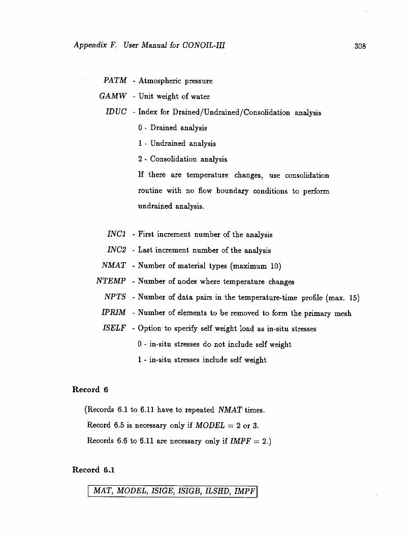
Appendix F. User Manual for CONOIL-IlI 308
PATM - Atmospheric pressure
GAMW - Unit weight of water
ID UC - Index for Drained/Undrained/Consolidation analysis
0 - Drained analysis
1 - Undrained analysis
2 - Consolidation analysis
If there are temperature changes, use consolidation
routine with no flow boundary conditions to perform
undrained analysis.
INCJ - First increment number of the analysis
1N02 - Last increment number of the analysis
NMAT - Number of material types (maximum 10)
NTEMP - Number of nodes where temperature changes
NPTS - Number of data pairs in the temperature-time profile (max. 15)
IPRIM - Number of elements to be removed to form the primary mesh
ISELF - Option to specify self weight load as in-situ stresses
0 - in-situ stresses do not include self weight
1 - in-situ stresses include self weight
Record 6
(Records 6.1 to 6.11 have to repeated NMAT times.
Record 6.5 is necessary only if MODEL 2 or 3.
Records 6.6 to 6.11 are necessary only if IMPF = 2.)
Record 6.1
MAT, MODEL, ISICE, 151GB, ILSHD, IMPF

Appendix F. User Manual for CONOIL-III 309
MAT - Material number
MODEL - Stress-Strain model type
1 - hyperbolic model
2 - modified Matsuoka’s model
3 - modified Matsuoka’s model with Cap-type yield
ISIGE - Option to calculate Young’s modulus
0 - use mean normal stress
1 - use minor principal stress
181GB - Option to calculate bulk modulus
0 - use mean normal stress
1 - use minor principal stress
ILSHD - Load transfer option
0 - do not perform load transfer
1 - perform load transfer
IMPF - Multi phase flow option
0 - fully saturated
1 - partially saturated
2 - three phase fluid flow (needs additional parameters)
Record 6.2 (all are real variables)
e,KE,n,Rf,KB,m,7,k,k,k2
e - Initial void ratio
KE - Elastic modulus constant
n - Elastic modulus exponent

Appendix F. User Manual for CONOIL-III 310
- Failure ratio
KB - Bulk modulus constant
m - Bulk modulus exponent
- total unit weight of soil
- permeability in x direction
- permeability in y direction
- permeability in z direction
if IMPF = 0 or 1 give the absolute permeability values (rn/s)
if IMPF = 2 give intrinsic permeability values (m2)
Record 6.3 (all are real variables)
c - Cohesion
- Friction angle at a confining pressure of 1 atmosphere
- Reduction in friction angle for a ten fold increase in
confining pressure
- strain softening constant
q - strain softening exponent
S - Initial degree of saturation (between 0 and 1, not in %)
- Saturation at which fluid begins to move freely. (used
to modify permeability for partially saturated soils. S1
generally close to zero)
B8 - Bulk modulus of the solids
B - Bulk modulus of the water
B0 - Bulk modulus of the oil
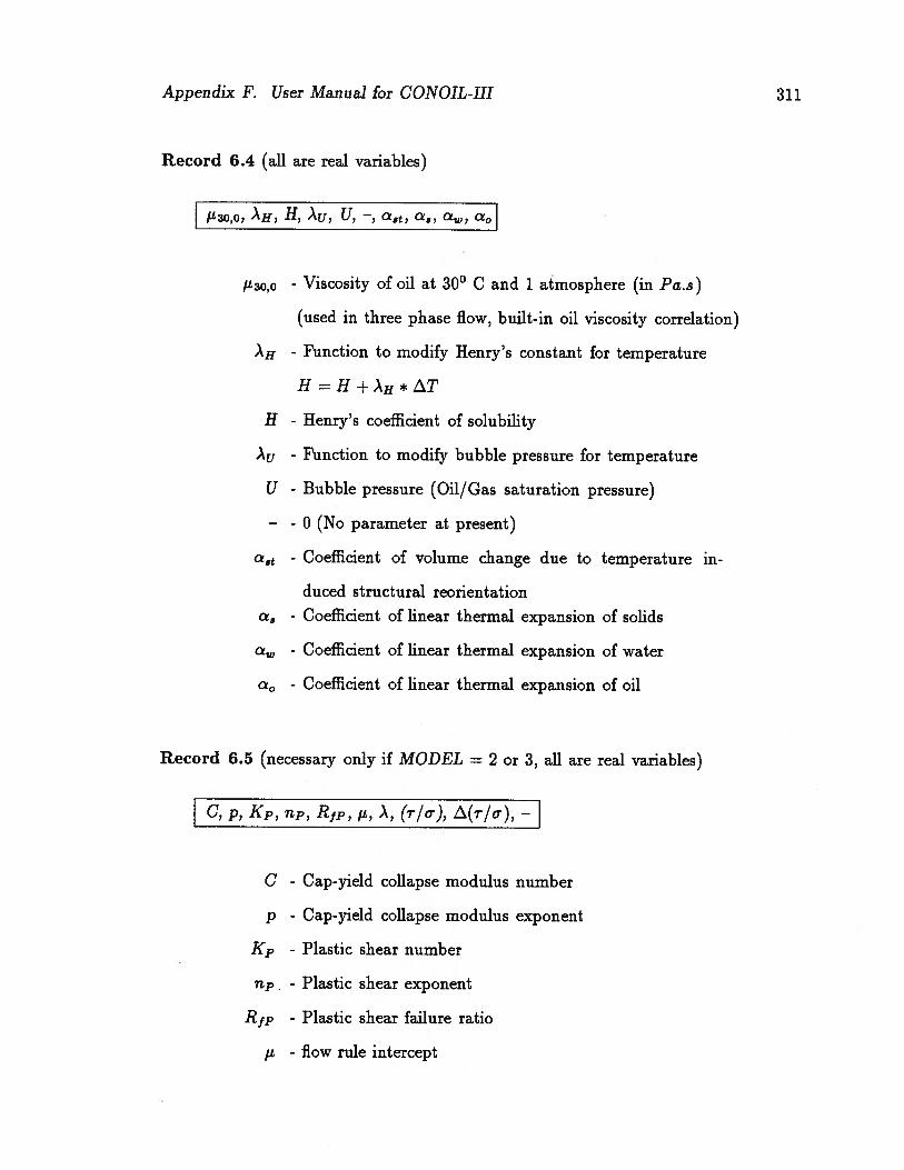
Appendix F. User Manual for CONOIL-III 311
Record 6.4 (all are real variables)
,U30,0, )H, H, Au, U, —, ant, c.z8, a, a0j
fL3o,o - Viscosity of oil at 300 C and 1 atmosphere (in Pa.s)
(used in three phase flow, built-in oil viscosity correlation)
- Function to modify Henry’s constant for temperature
H=H+AH*T
H - Henry’s coefficient of solubility
Au - Function to modify bubble pressure for temperature
U - Bubble pressure (Oil/Gas saturation pressure)
—
- 0 (No parameter at present)
a8t - Coefficient of volume change due to temperature in
duced structural reorientation- Coefficient of linear thermal expansion of solids
- Coefficient of linear thermal expansion of water
a0 - Coefficient of linear thermal expansion of oil
Record 6.5 (necessary only if MODEL = 2 or 3, all are real variables)
C, p, K, rip, R1p, i, A, (r/), (r/o),—
C - Cap-yield collapse modulus number
p - Cap-yield collapse modulus exponent
K - Plastic shear number
lip - Plastic shear exponent
R1 - Plastic shear failure ratio
- flow rule intercept
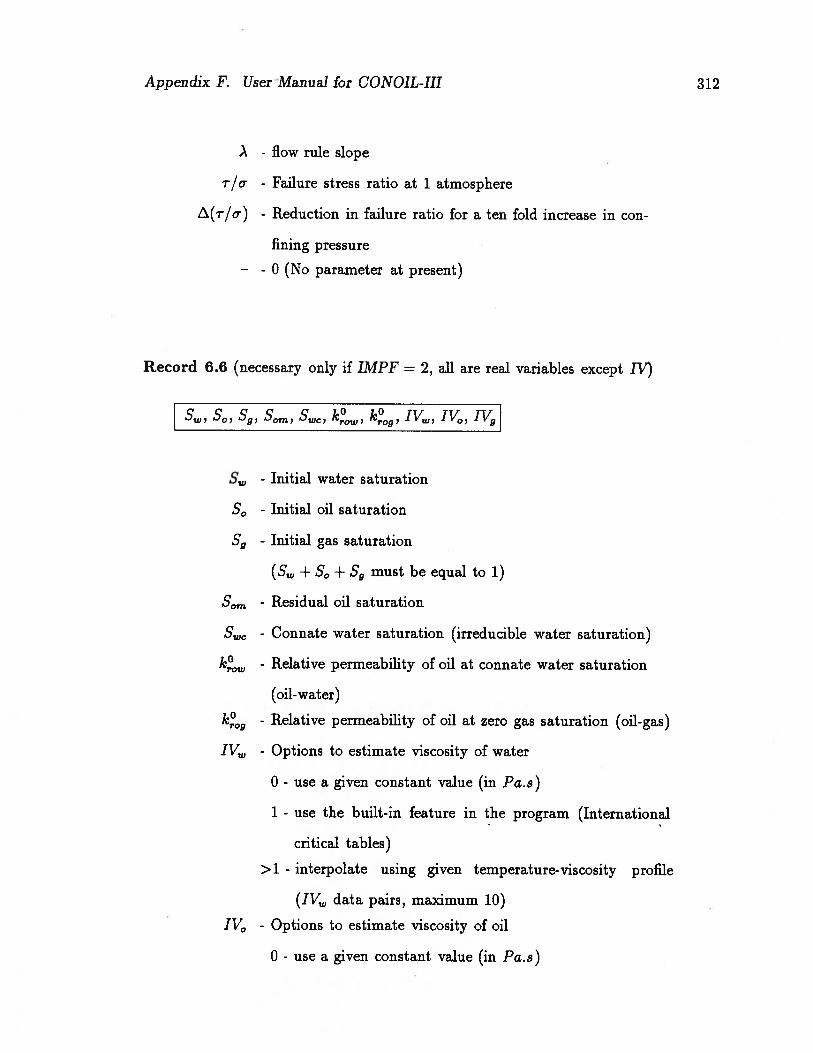
Appendix F. User Manual for CONOIL-III 312
A - flow rule slope
r/o- - Failure stress ratio at 1 atmosphere
- Reduction in failure ratio for a ten fold increase in con
fining pressure—
- 0 (No parameter at present)
Record 6.6 (necessary only if IMPF = 2, all are real variables except IV)
Sw, So, S, Sam, Swc, 1ow, ‘og IVj
S,, - Initial water saturation
S0 - Initial oil saturation
S9 - Initial gas saturation
(S + S0 H- S9 must be equal to 1)
S - Residual oil saturation
S - Connate water saturation (irreducible water saturation)
- Relative permeability of oil at connate water saturation
(oil-water)
k,?09 - Relative permeability of oil at zero gas saturation (oil-gas)
IV,, - Options to estimate viscosity of water
0 - use a given constant value (in Fa.s)
1 - use the built-in feature in the program (International
critical tables)
>1 - interpolate using given temperature-viscosity profile
(IV data pairs, maximum 10)
1V0 - Options to estimate viscosity of oil
0 - use a given constant value (in Pa.s)

Appendix F. User Manual for CONOIL-III 313
1 - use the built-in feature in the program (Correlation by
Puttangunta et.al (1988), to,o should be given in record
6.4)
>1 - interpolate using given temperature-viscosity profile
(1V0 data pairs, maximum 10)
1V9 - Options to estimate viscosity of gas
0 - use a given constant value (in Pa..s)
1 - use the built-in feature in the program (a constant value
2.E-5 Pa.s)
>1 - interpolate using given temperature-viscosity profile
(1V9 data pairs, maximum 10)
Record 6.7 (necessary only if IMPF = 2)
Al, A2, A3, Bi, B2, B3, Cl, 02, 03, Dl, D2, D3
Al.. .A3 - Parameters for relative permeability of water (oil-water)
= A1(SL, — A2)-3
Bl...B3 - Parameters for relative permeability of oil (oil-water)
= B1(B2 —
Cl... C3 - Parameters for relative permeability of gas (oil-gas)
ICrg = C1(Sg —
Dl...D3 - Parameters for relative permeability of oil (oil-gas)
k,.09 = D1(D2 S9)”3
Record 6.8 (necessary only if IMPF = 2)
Fl, F2, F3
Fl...F3 - Parameters for oil-gas capillary pressure

Appendix F. User Manual for CONOIL-III 314
of gas (oil-gas)
Pc = Fl Pa(Sg — F2)F3
Record 6.9 (necessary only if IMPF = 2 and IV,, = 0 or >1)
V (ifIV=0)
Vi, Ti, V2, T2,... (if IV 1, IV, data pairs, maximum 10)
Vi,, - Constant viscosity value of water (in Pa.s)
Vi,... - Viscosity values in the given profile (in Pa.s)
Ti,... - Temperature values in the given profile (in °C)
Record 6.10 (necessary only if IMPF = 2 and 1V0 = 0 or >1)
___
(ifIV0=0)
Vi, Ti, V2, T2,... (if 1V0 > 1, IV,, data pairs, maximum 10)
V0 - Constant viscosity value of oil (in Pa.s)
Vi,... - Viscosity values in the given profile (in Fa.s)
Ti,... - Temperature values in the given profile (in °C)
Record 6.11 (necessary only if IMPF = 2 and IVg = 0 or >1)
___
(ifIV=0)
Vi, Ti, V2, T2,... (if 1V9> 1, 1V9 data pairs, maximum 10)
- Constant viscosity value of gas (in Pa.s)
Vi,... - Viscosity values in the given profile (in Pa.s)
Ti,... - Temperature values in the given profile (in °C)
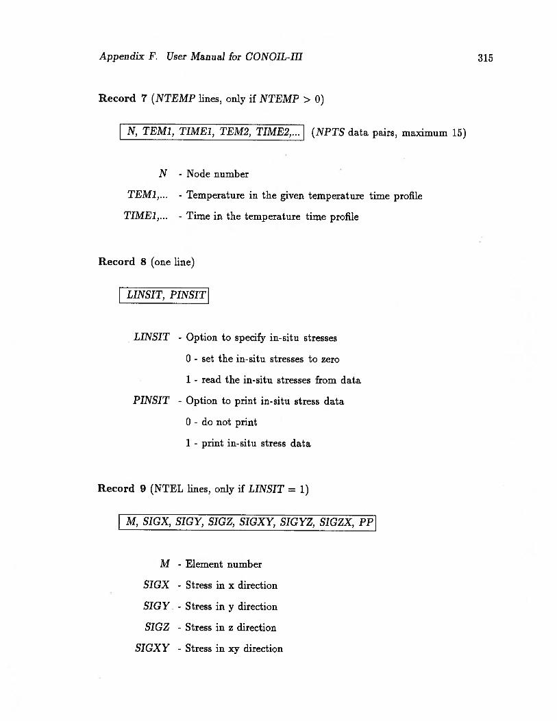
Appendix F. User Manual for CONOIL-III 315
Record 7 (NTEMP lines, only if NTEMP > 0)
TEM1, TIME1, TEM2, TIMEj (NPTS data pairs, maximum 15)
N - Node number
TEM1,... - Temperature in the given temperature time profile
TIMEJ,... - Time in the temperature time profile
Record 8 (one line)
LINSIT, PINSIT
LINSIT - Option to specify in-situ stresses
o - set the in-situ stresses to zero
1 - read the in-situ stresses from data
PINSIT - Option to print in-situ stress data
o - do not print
1 - print in-situ stress data
Record 9 (NTEL lines, only if LINSIT = 1)
M, SIGX, SIGY, SIGZ, SIGXY, SIGYZ, SIGZX, PP1
M - Element number
SIGX - Stress in x direction
SIGY - Stress in y direction
SIGZ - Stress in z direction
SIGXY - Stress in xy direction

Appendix F. User Manual for CONOIL-III 316
SIGYZ - Stress in yz direction
SIGZX - Stress in zx direction
PP - Pore pressure
Record 9 has to be repeated for all elements. If elements cards are omitted, the
stresses for a series of elements are generated by assigning the same stresses as the
previous element. Stresses for the first and the last elements must be specified.
Record 10 ((IPRIM-1)/10 + 1 lines, only if IPRIM> 0)
Li, L2,...
Li,... - List of element numbers to be removed to form mesh at
the beginning of the analysis (LPPJM element numbers)
There must be 10 data per line, except the last line
Record 11
(one line, records 11 to 14 have to be repeated for incre
ments from INC1 to INC2)
INC, ICHEL, NLOAD, NFIX, 10 UT, DTIME, DGRAV
INC - Increment number
ICHEL - Number of elements to be removed from primary mesh
NLOAD - Number of nodes where loads are applied
NFIX - Number of nodes where nodal fixities are changed
lOUT - Option for printing results (5 digit code ‘ abcde’)
a = 1 print nodal displacements
b = 1 print moduli values and saturations

Appendix F. User Manual for CONOIL-IlI 317
c = 1 print strains and coordinates of the integration point
where results are printed
d = 1 print stresses and pore pressure
e = 1 print velocity vectors
DTIME - Time increment
DGRAV - Increase in gravity
Record 12 ((ICH.EL-1)/10 + 1 lines, only if ICHEL > 0)
Li, L2
Li,... - List of element numbers to be removed in this increment
There must be 10 data per line, except the last line
Record 13 (NLOAD lines, only if NLOAD> 0)
N, DFX, DFY, DFZI
N - Node number
DFX - Increment in x force
DFY - Increment in y force
DFZ - Increment in z force
Record 14 (NFIX lines, only if NFIX> 0)
N, NFCODE, DX, DY, DZ, DP
N - Node number

Appendix F. User Manual for CONOIL-III 318
NFCODE - Four digit code ‘abcd’ which specifies the fixity condi
tions associated with the nodea = 0 free in x direction
= 1 will have prescribed incremental displacement DX
b = 0 free in y direction
= 1 will have prescribed incremental displacement DY
c = 0 free in z direction
= 1 will have prescribed incremental displacement DZ
d = 0 pore pressure can have any value (undrained boundary)
= 1 will have prescribed incremental pore pressure DP
= 2 will have zero absolute pore pressure for this and all
subsequent increments
DX - Prescribed displacement in x direction
DY - Prescribed displacement in y direction
DZ - Prescribed displacement in z direction
DP - Prescribed pore pressure

Appendix F. User Manual for CONOIL-IlI 319
F.3 Example Problem 1
An example of a general stress analysis under one dimensional loading is illustrated
here. The material is assumed to be linear elastic. The finite element mesh consists
of two brick elements as shown in figure F.2. The data file and the corresponding
output file from the program are given in subsections.
25 kN
H G
Ei‘12
6...I
0ZL
ol...
AB, BC, CD, DA - Totally Fixed
AE, BF, CG, DH - Vertically Free
Figure F.2: Finite element mesh for example problem 1
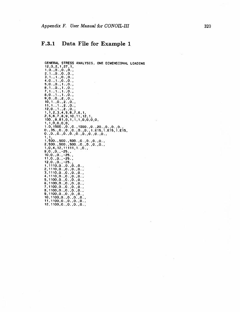
“O”O”OO’OOLLL“O”O”O”O’OOLLLL“O”O”O”000LL01“O”O”O”OOOLL6
0”O”O”OOOLL’8“O”O”O”OOOU.L
OOO”OOOL.V9O”O”O”OOOLL9
“OOO0’OLLLV•.0000’OLLLE“O”O”O”O’OILL“O”O”O”O’OLLLL
S-”O”O’LS-O”OLL
S-”O”O6Q’‘LLLLLIV’OL
“o”o”o”o”oog”oog”oog’••O••O••O••O•OOS•OOS’OOS’L
LL‘•o••o••o’•o•o’•o••o•o•o
SL3L’SL3LS3LOOO”O”O”sOOO”O”OOOOOO”O”OOLOL
0000LL‘O’000Lt096’OOL
‘L’LLLOL68L99‘L8L9S’V’Li
0LOL‘OL’L’LL
O”O”LOL“O”O”O6o”VL”o9“O”L”I.”L1“O”L”O”L9“O•L009“O”O”L”0V“O”O”L”LE
“o”o”o”oH•LLLOL
ONIOVO71VNOISN3YUO3N0SISA1VNVSS3UISVH3N35
jIdmxaiojuir
111710N00io;nuvJjisfljxrpudd

EL
EM
EN
T-N
OD
AL
INFO
RM
AT
ION
NO
DE
SE
LE
.N
O.
12
34
56
78
o CD ‘•l
—C
)U
11
23
45
67
82
56
78
910
1112
MA
TE
RIA
LP
RO
PE
RT
IES
MA
TE
RIA
LI
=
MO
DEL
NIS
IGE
ISIG
BIL
SH
DI
MPF
LIN
EA
R/N
ON
LIN
EA
RE
LA
ST
ICM
OD
ELU
SEM
EAN
NO
RM
AL
ST
RE
SS
USE
MEA
NN
OR
MA
LS
TR
ES
SN
OLO
AD
SHE
DD
ING
FUL
LY
SAT
UR
AT
ED
SO
IL
O.1
00E
+O
10.1
50E
+04
O.0
00E
÷O
OO
.000
E+
OO
0.1
00
E+
04
O.0
00E
÷O
OO
.200E
+O
2O
.000
E+
OO
O.0
00E
+O
OO
.00
0E
+O
OO
.000E
÷O
OO
.350E
+02
O.0
00E
÷O
OO
.000
E+
OO
O.0
00E
+O
OO
.000E
+O
OO
.000
E+
OO
O.1
00
E+
16
0,1
00
E+
16
O.1
00E
+16
O.0
00
E+
OO
O.0
00E
+O
OO
.000
E+
OO
O.0
00E
+O
OO
.OO
OE
OO
O.0
00E
+O
OO
.000
E+
OO
O.0
00E
+O
OO
.00
0E
+O
OO
.000E
+O
0
•A
OFO
IL
(A)N
AL
YS
ISO
F(D
)EF
OR
MA
TIO
NA
ND
(F)L
OW
IN(O
IL)
SAN
DS
GE
NE
RA
LS
TR
ES
SA
NA
LY
SIS
,O
NE
DIM
EN
SIO
NA
LL
OA
DIN
G
NO
DA
LC
OO
RD
INA
TE
SA
ND
TE
MPE
RA
TU
RE
NO
DE
XC
OO
RD
Y-C
OO
RD
Z-C
OO
RD
TEM
P
10
.00
00000
0.0
00
0.0
00
21
.00
00.0
00
0.0
00
0.0
00
31
.00
01.0
00
0.0
00
0.0
00
40
.00
01
.00
00.0
00
0.0
00
50
.00
00
.00
01.0
00
0.0
00
61
.00
00
.00
01.0
00
0.0
00
71
.00
01
.00
01.0
00
0.0
00
80
.00
01.0
00
1.0
00
0.0
00
90
.00
00
.00
02
.00
00.0
00
101
.00
00
.00
02
.00
00.0
00
111
.00
01
.00
02
.00
00.0
00
120.0
00
1.0
00
2.0
00
0.0
00
=0
=0
=0
=0
L’3
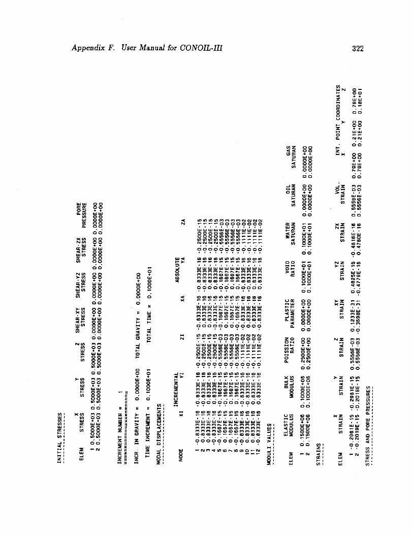
INIT
IAL
ST
RE
SS
ES X
EL
EM
ST
RE
SS
1O
.5000E
+03
2O
.50
00
E+
03
INC
RE
ME
NT
NU
MB
ER=
VZ
SHE
AR
-XY
SHE
AR
-YZ
SHE
AR
-ZX
POR
ES
TR
ES
SS
TR
ES
SS
TR
ES
SS
TR
ES
SS
TR
ES
SPR
ESS
UR
E
O.5
000E
+03
O.5
000E
+03
O.0
000E
+O
OO
.0000E
+O
OO
.0000E
+O
OO
.000
0E+
OO
O.5
OO
OE
O3
O.5
00
0E
+03
O.0
000E
+O
OO
.0000E
+O
OO
.0000E
+O
OO
.0000E
+O
O
INC
H.
ING
RA
VIT
Y=
0.0
00
0E
÷O
OTO
TAL
GR
AV
ITY
=O
.00
00
E+
O0
TIM
EIN
CR
EM
EN
T=
O.1
000E
+O
1TO
TAL
TIM
E=
O.1
000E
+O
1
NO
DA
LD
ISPL
AC
EM
EN
TS
I-s
NO
DE
XI
ZI
XA
1-0
.8333E
-16
-O.8
333E
-16
02
O.8
333E
-16
O.8
33
3E
-16
3O
.8333E
-16
O.8
33
3E
-16
4-O
.8333E
-16
-O.8
333E
-16
5-O
.16
67
E-1
5-O
.1667E
-15
6O
.1667E
-15
O.1
66
7E
-15
7O
.1667E
-15
O.1
66
7E
-15
8-O
.16
67
E-1
5-O
.1667E
-15
9-O
.8333E
-16
-O.8
333E
-16
10O
.8333E
-16
O.8
33
3E
-16
11O
.8333E
-16
O.8
33
3E
-16
12-O
.8333E
-16
-O.8
333E
-16
MO
DU
LIV
AL
UE
S
PL
AS
TIC
PAR
AM
ET
ER
0.0
000E
+O
O0.
00
00
E+
0O
INC
RE
ME
NT
AL VI
-O.8
333E
-16
-0.8
333E
-16
0.B
333E
-16
0.8
333E
-16
-0.
1667E
-15
-0.
1667E
-15
0.
16
67
E-
150
.1
66
7E
-15
-O.8
333E
-16
-O.8
333E
-16
O.8
333E
-16
O.8
333E
-16
BU
LKM
OD
ULU
S
0.
1000E
+06
0.
1000E
+06 V
ST
RA
IN
-O.2
981E
-15
-D.2
019E
-15
AB
SOL
UT
E VA
-O.8
333E
-16
-O.8
33
3E
-16
0.8
333E
-16
O.8
333E
-16
-0.
1667E
-15
-0.
1667E
-15
0.
1667E
-15
0.
1667E
-15
-O.8
333E
-16
-O.8
333E
-16
O.8
33
3E
-16
O.8
33
3E
-16
VO
IDR
AT
IO
0.
I00
0E
+0
10.
1000E
+01
ELEM
2
ZA
-O.2
500E
-15
-0.
2500E
-15
-O.2
500E
-15
-O.2
500E
-15
-0.
55
56
E-0
3O
.55
56
E-0
3-0
.5
55
6E
-03
•O.5
556E
-O3
-0.
1111E
-O2
-0.
1111E
-02
-0.1
11
IE-0
2-0
.11
11
E-0
2
WA
TER
SAT
UR
AN
0.
I000
E+
O1
0.
1000
E+
O1
EL
AS
TIC
MO
DU
LUS
0.
1500E
+06
0.
1500
E+
O6
-O.2
500E
-15
0.2
500E
-15
-0.
2500E
-15
-O.2
500E
-15
-0.
5556E
-03
-O.5
55
6E
-O3
-0.5
55
6E
-03
-O.5
556E
-O3
-0.
1111E
-O2
-0.
11
11
E-0
2-0
.11
11E
-O2
-0.1
11
1E
-02
PO
ISS
ION
RA
TIO
0.2
500E
+O
00.
25
00
E+
00 Z
ST
RA
IN
0.5
55
6E
-O3
O.5
55
6E
-03
ST
RA
INS
EL
EM 2
XS
TR
AIN
-O.2
981E
-15
-0.
20lY
E-
15
OIL
SAT
UR
AN
0.0
000E
+O
0O
.0000E
+0
0
XVY
ZS
TR
AIN
ST
RA
IN
GA
SSA
TU
RA
N
0.
0000
E+
OO
0.
00
00
E+
00
TN
T.
PO
INT
CO
OR
DIN
AT
ES
XV
ZZX
VO
L.
ST
RA
INS
TR
AIN
0.1
23
3E
-31
O.4
82
5E
-16
-O.4
816E
-16
O.5
55
6E
-03
O.7
9E
+0O
0.2
1E
+00
O.7
9E
+0O
-0.3
69
8E
-31
-0.4
77
9E
-16
O.4
78
0E
-16
0.5
55
6E
-03
O.7
9E+
OO
0.2
1E
+00
0.1
8E
+0
lC
3
I.3
ST
RE
SS
AN
DPO
RE
PR
ES
SU
RE
S
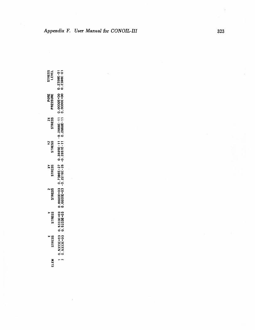
XV
ZXV
YZ
ZXPO
RE
ST
RE
SS
EL
EM
ST
RE
SS
ST
RE
SS
ST
RE
SS
ST
RE
SS
ST
RE
SS
ST
RE
SS
PRE
SSU
RE
LE
VE
L
1O
.53
33
E-O
3O
.5333E
+03
O.6
000E
+03
O.7
396E
-27
O.8
95E
-11
-O.2
88
9E
-11
O.0
00
0E
+O
OO
.23
98
E-O
1O
.53
33
E+
O3
O.5
33
3E
+03
O.6
000E
+03
-O.2
219E
-26
-O.2
86
7E
-11
O.2
868E
-I1
O.0
00
0E
+O
OO
.23
g8
E-O
rj I
Copyright © 2022 FDOKUMEN