Singular Elasto-Static Field Near a Fault Kink

RODRIGO ARIAS,1 RAUL MADARIAGA,2 and MOKHTAR ADDA-BEDIA3

Abstract—We study singular elastic solutions at an angular

corner left by a crack that has kinked. We have in mind a geo-

physical context where the faults on either side of the kink are

under compression and are ready to slip, or have already slipped,

under the control of Coulomb friction. We find separable static

singular solutions that are matched across the sides of the corner by

applying appropriate boundary conditions. In our more general

solution we assume that one of the sides of the corner is about to

slide, i.e. it is just contained by friction, and the other may be less

pressured. Our solutions display power law behaviour with real

exponents that depend continuously on the angle of the corner, the

coefficient of static friction and the difference of shear load on both

sides of the corner. When friction is the same on both sides of the

kink, the solutions split into a symmetric and an antisymmetric

solution. The antisymmetric solution corresponds to the simple

shear case; while the symmetric solution appears when the kink is

loaded by uniaxial stress along the bisector of the kink. The anti-

symmetric solution is ruled out under this model with contact since

the faults cannot sustain tension. When one side of the corner is

less pressured one can also distinguish modes with contact overall

from others that must open up on one side. These solutions provide

an insight into the stress distributions near fault kinks, they can also

be used as tools for improving the numerical calculation of kinks

under static or dynamic loads.

1. Introduction

Kinks and other geometrical discontinuities play

an essential role in the control of rupture propagation

along natural faults as discussed by SIBSON (1985) and

many others. The study of rupture propagation along

a seismic fault containing one or more kinks, jogs,

bends or discontinuities has been examined by many

authors (see, e.g., SEGAL and POLLARD, 1980; KING and

NABELEK, 1985; HARRIS and DAY, 1999; POLIAKOV

et al., 2002; KAME and YAMASHITA, 1999;KAME et al.,

2003). Most of those studies did not explicitly

address the problem of the stress distribution near the

kink or bend because the main concern was the study

of rupture propagation. The stress field left by frac-

ture propagation that has kinked plays a fundamental

role in the energy balance of the fault, it will produce

strong radiation and could stop or favor rupture

propagation.

The first study of the mechanical problems posed

by a kink or bend in active faults was presented by

ANDREWS (1989) in the static approximation. He

realized that kinks posed a geometrical problem and

they could not remain stable under finite deformation.

He then modeled a particular example of a kink and

found that stresses became singular at the cusp. Fol-

lowing this study, many authors have examined the

role of kinks on faulting from different perspectives.

In the static approximation a major step was accom-

plished by TADA and YAMASHITA (1997), who found

that the tip of the kink produced a stress singularity

that depended on the way the tip was smoothed. In the

dynamic approximation, a propagating shear crack

fault with kinks has been modeled by OGLESBY et al.

(2003); AOCHI et al. (2000) and many others.

In the dynamic approximation most of the work

has been numerical, but in many of these simulations

the approximation of the stress field and the boundary

conditions in the immediate vicinity of the kink poses

problems. ADDA-BEDIA and ARIAS (2003) and ADDA-

BEDIA and MADARIAGA (2008) solved the problem of a

Mode III crack propagating along a fault that has a

kink. They showed that the solution of this problem

was intimately related to the singularity of the static

stress field in the vicinity of the kink. The static

problem for the antiplane kink was solved by SIH

(1965) using the eigenvalue methods proposed by

1 Departamento de Fısica, FCFM, Universidad de Chile,

Santiago, Chile. E-mail: rarias@dfi.uchile.cl2 Laboratoire de geologie, CNRS-Ecole Normale Superieure,

Paris, France. E-mail: madariag@geologie.ens.fr3 Laboratoire de physique statistique, CNRS-Ecole Normale

Superieure, Paris, France. E-mail: adda@lps.ens.fr

Pure Appl. Geophys. 168 (2011), 2167–2179

� 2011 Springer Basel AG

DOI 10.1007/s00024-011-0298-y Pure and Applied Geophysics

WILLIAMS (1952). For the in-plane or Mode II faults,

the problem of the stress and displacement distribu-

tion does not seem to have been discussed in the

literature except for the previous cited works by

ANDREWS (1989) and TADA and YAMASHITA (1997).

In this paper we study a Mode II shear crack that

has a kink at its center. When the crack abruptly

changes its direction of propagation, it leaves behind

a corner region that plays a characteristic role in the

global elastic behavior. It is pertinent to study the

nature of the elastic fields in this region since one

expects the fields may develop singular behavior that

is interesting by itself, and also because numerical

simulations in geometries with these corners require

knowledge of singular behaviors in order to be

accurate and efficient.

We approach the problem of finding all possible

singular and regular elastic solutions in the region close

to these corners in an isotropic homogeneous elastic

medium. We have in mind kinks that occur in seismic

contexts, i.e. the corner sides are in contact and under

compression. This raises the issue of the role of friction

on the elastic solutions: we will explore static solutions

in which at least one of the sides of the corner is about to

give way under the prevailing local shear. We found

singular power law solutions in the regions of the

corner that have real exponents. The latter exponents

depend continuously on the angle of the corner, the

coefficient of friction and the degree of stress of the

side of the corner that may not be about to give way.

These exponents are universal in the sense that they

depend on the elastic properties of the medium.

The seminal paper in the study of elastic angular

corners is the one of WILLIAMS (1952), where he

studied an angular corner with free sides, finding a

solution separable in polar coordinates. Here, we use

analogous solutions by SEWERYN and MOLSKI (1996)

as starting points (they studied angular corners under

various boundary conditions), and we match solutions

of these types on both sides of the kink corner by use

of appropriate boundary conditions.

2. Singular Elastic Fields at Kinks

We consider a Mode II shear crack with a kink

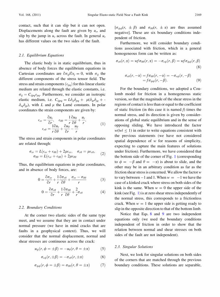
and we will focus at the corner region. The geometry

is shown in Fig. 1. The crack separates two infinite

homogeneous elastic wedges with identical elastic

properties. Since we are interested in the stress field

in the vicinity of the cusp we consider that the two

faults on the side of the kink extend to infinity. In the

cusp of the kink we impose no smoothing. In the

terminology of BARENBLATT (1996) this is the inter-

mediate asymptotic solution to the two wedges in

frictional contact across the fault. Although we will

not do this, the near cusp asymptotic field can be

studied using a local approximation (see TADA and

YAMASHITA, 1997). In wedge 1 we use a coordinate

system (r, h) centered on the bisector to the kink (hincreases anti-clockwise), and on wedge 2 we use a

coordinate system (r, /), in which / increases

clockwise (see Fig. 1). The fault is assumed to be in

Figure 1Geometry of a shear crack with a kink. In medium 1, to the right,

we use a coordinate system (r, h). In medium 2, to the left, we use a

coordinate system (r, /). The two media are in frictional contact

at h = a, / = b (as well as at h = -a, / = -b), so that

a = p - b

2168 R. Arias et al. Pure Appl. Geophys.

contact, such that it can slip but it can not open.

Displacements along the fault are given by ur, and

slip by the jump in ur across the fault. In general ur

has different values on the two sides of the fault.

2.1. Equilibrium Equations

The elastic body is in static equilibrium, thus in

absence of body forces the equilibrium equations in

Cartesian coordinates are qrij/qxj = 0, with rij the

different components of the stress tensor field. The

stress and strain components ð�pqÞ for this linear elastic

medium are related through the elastic constants, i.e.

rij ¼ Cijpq�pq: Furthermore, we consider an isotropic

elastic medium, i.e. Cijpq = Ldijdpq ? l(dipdjq ? -

diqdjp), with L and l the Lame constants. In polar

coordinates the strain components are given by:

�rr ¼our

or; �hh ¼

1

r

ouh

ohþ ur

r;

�rh ¼1

r

our

ohþ ouh

or� uh

r

ð1Þ

The stress and strain components in polar coordinates

are related through:

rrr ¼ Lð�rr þ �hhÞ þ 2l�rr; rrh ¼ l�rh;rhh ¼ Lð�rr þ �hhÞ þ 2l�hh

ð2Þ

Thus, the equilibrium equations in polar coordinates,

and in absence of body forces, are:

0 ¼ orrr

orþ 1

r

orrh

ohþ rrr � rhh

rð3Þ

0 ¼ orrh

orþ 1

r

orhh

ohþ 2

rrrh ð4Þ

2.2. Boundary Conditions

At the corner two elastic sides of the same type

meet, and we assume that they are in contact under

normal pressure (we have in mind cracks that are

faults in a geophysical context). Thus, we will

consider that the normal displacement, normal and

shear stresses are continuous across the crack:

u/ðr;/ ¼ �bÞ ¼ �uhðr; h ¼ �aÞ ð5Þ

rr/ðr;�bÞ ¼ �rrhðr;�aÞ ð6Þ

r//ðr;/ ¼ �bÞ ¼ rhhðr; h ¼ �aÞ ð7Þ

[r//(r, ± b) and rhh(r, ± a) are thus assumed

negative]. These are six boundary conditions inde-

pendent of friction.

Furthermore, we will consider boundary condi-

tions associated with friction, which in a general

homogeneous form can be written as:

rrhðr; aÞ ¼ wfrhhðr; aÞ ¼ �rr/ðr; bÞ ¼ wf r//ðr; bÞð8Þ

rrhðr;�aÞ ¼ f rhhðr;�aÞ ¼ �rr/ðr;�bÞ¼ f r//ðr;�bÞ: ð9Þ

For the boundary conditions, we adopted a Cou-

lomb model for friction in a homogeneous static

version, so that the magnitude of the shear stress in the

regions of contact is less than or equal to the coefficient

of static friction (in this case it is named f) times the

normal stress, and its direction is given by consider-

ations of global static equilibrium and in the sense of

opposing sliding. We have introduced the factor

w(|w| B 1) in order to write equations consistent with

the previous statements (we have not considered

spatial dependence of w for reasons of simplicity,

expecting to capture the main features of solutions

under friction). Furthermore, we have considered that

the bottom side of the corner of Fig. 1 (corresponding

to / = -b and h = -a) is about to slide, and the

other may be in an arbitrary condition as far as the

friction shear stress is concerned. We allow the factor w

to vary between -1 and 1. When w = -1 we have the

case of a kinked crack where stress on both sides of the

kink is the same. When w = 0 the upper side of the

kink (see Fig. 1) is at zero shear stress independently of

the normal stress, this corresponds to a frictionless

crack. When w = 1 the upper side is getting ready to

slip in the opposite direction to that of the bottom limb.

Notice that Eqs. 8 and 9 are two independent

equations only (we used the boundary conditions

independent of friction in order to show that the

relation between normal and shear stresses on both

sides of the fault are not independent).

2.3. Singular Solutions

Next, we look for singular solutions on both sides

of the corners that are matched through the previous

boundary conditions. These solutions are separable,

Vol. 168, (2011) Singular Elasto-static Field Near a Fault Kink 2169

with radial power law behaviour, and sinusoidal

angular behaviour, and correspond to the fundamen-

tal solutions originally proposed by WILLIAMS (1952)

(of the type ur = rkh(h) and uh = rkg(h), with k and

exponent to be determined). The particular version of

the potentials that we use are those of SEWERYN and

MOLSKI (1996). These solutions for the displacement

and stress fields, close to the corner and for the elastic

medium (1) to the right are written as:

ur ¼ rk½Acosðð1þ kÞhÞ þ Bsinðð1þ kÞhÞþ Ccosðð1� kÞhÞ þ Dsinðð1� kÞhÞ�

ð10Þ

uh ¼ rk½Bcosðð1þ kÞhÞ � Asinðð1þ kÞhÞþ m2Dcosðð1� kÞhÞ � m2Csinðð1� kÞhÞ�

ð11Þ

rhh ¼ rk�1l½�2kAcosðð1þ kÞhÞ � 2kBsinðð1þ kÞhÞ� ð1þ kÞð1� m2ÞCcosðð1� kÞhÞ� ð1þ kÞð1� m2ÞDsinðð1� kÞhÞ� ð12Þ

rrh ¼ rk�1l½2kBcosðð1þ kÞhÞ � 2kAsinðð1þ kÞhÞþ ð1� kÞð1� m2ÞDcosðð1� kÞhÞ� ð1� kÞð1� m2ÞCsinðð1� kÞhÞ� ð13Þ

And similarly, on medium (2) to the left side:

ur ¼ rk½acosðð1þ kÞ/Þ þ bsinðð1þ kÞ/Þþ ccosðð1� kÞ/Þ þ dsinðð1� kÞ/Þ�

ð14Þ

u/ ¼ rk½bcosðð1þ kÞ/Þ � asinðð1þ kÞ/Þþ m2dcosðð1� kÞ/Þ � m2csinðð1� kÞ/Þ�

ð15Þ

r// ¼ rk�1l½�2kacosðð1þ kÞ/Þ� 2kbsinðð1þ kÞ/Þ� ð1þ kÞð1� m2Þccosðð1� kÞ/Þ� ð1þ kÞð1� m2Þdsinðð1� kÞ/Þ� ð16Þ

rr/ ¼ rk�1l½2kbcosðð1þ kÞ/Þ � 2kasinðð1þ kÞ/Þþ ð1� kÞð1� m2Þdcosðð1� kÞ/Þ� ð1� kÞð1� m2Þcsinðð1� kÞ/Þ� ð17Þ

with l the shear modulus, m = L/(2(L ? l)) Pois-

son’s ratio, L Lame’s first parameter, m2 : (3 ? k -

4m)/(3 - k - 4m), and k an exponent to be deter-

mined by the boundary conditions as well as the

different coefficients A, B, C, D, a, b , c , d (except

for a constant factor, since these are linear solutions).

The boundary condition Eqs. 5–9 are effectively

eight homogeneous equations for the eight unknown

coefficients A, B, C, D, a, b , c , d. Thus, they have

non zero solutions only for specific values of the

singular exponent k. In principle the eigenvalue

equation for k could be obtained by imposing that the

corresponding 8 9 8 determinant to be null. But, due

to symmetry considerations and other algebraic

simplifications it is better to proceed otherwise: the

details on how this eigenvalue equation (Eq. 55) is

derived are left to the Appendix.

Next we reproduce the just mentioned eigenvalue

equation, Eq. 55:

0 ¼ 4cos2ðkpÞ þ ½f ðwþ 1Þð1þ kÞsinð2WÞcosð2WkÞ�2

� ½2cosð2WÞcosð2WkÞ � 2ksinð2WÞsinð2WkÞþ f ð1� wÞð1þ kÞsinð2WÞcosð2WkÞ�2;

ð18Þ

where W � ðb� aÞ=2: This is an eigenvalue equation

for the determination of the power-law exponent k, it

takes the form 0 ¼ gðk;W; f ;wÞ. For each value of

the parameters, i.e. angle W, weight w and coefficient

of friction f, there is an infinite family of generally

complex eigenvalues (we inferred this by using the

method introduced in Sect. 2.5). Its solutions turn out

to be real in the range of k of more interest: the most

singular eigenvalues in the range 0.5 B Re(k) \ 1. In

general, when Re(k) C 1 the stress and displacement

fields are regular, when Re(k) \ 0.5 the stress field in

the vicinity of the kink has a strain energy concen-

tration that could only be produced by an external

source located at the cusp; while for Re(k) = 0.5 the

cusp behaves like a crack that stores a finite amount

of energy in its neighborhood. Thus, we will analyze

solutions in the range 0.5 B Re(k) \ 1. However,

there are some works where the region close to the tip

has been modeled (e.g. plasticity, nonlinear elasticity)

and this may allow for higher order singularities (see,

e.g., LABOSSIERE and DUNN, 2001, BOUCHBINDER et al.,

2009).

2.4. Special Cases

The special cases that we will present, i.e. the

frictionless corner and the case in which both sides

2170 R. Arias et al. Pure Appl. Geophys.

are about to slide, correspond to cases in which the

matrix of the eigenvalue equation (52) is diagonal.

2.4.1 Special Case, the Frictionless Corner

If the kink slips without friction, f = 0 in Eqs. 8 and

9. In this case the normal and shear stresses on the

sides of the kink are independent and we can assume

that shear stresses drop to zero independently of

normal stresses (an arbitrary continuous stress field

that satisfies the equilibrium conditions and that has

zero shear stress on the faults can be superimposed on

top of the solution we investigate here). We study the

frictionless kink in detail because it illustrates the

origin of the stress field in the vicinity of the kink.

In the absence of friction (f = 0), the eigenfunc-

tions separate into two separate families. One

solution is symmetric about the bisector of the kink

(x axis of Fig. 1), and the other is antisymmetric.

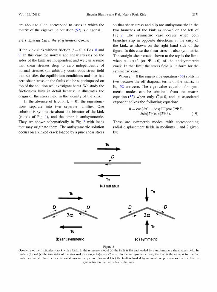
They are shown schematically in Fig. 2 with loads

that may originate them. The antisymmetric solution

occurs on a kinked crack loaded by a pure shear stress

so that shear stress and slip are antisymmetric in the

two branches of the kink as shown on the left of

Fig. 2. The symmetric case occurs when both

branches slip in opposite directions at the cusp of

the kink, as shown on the right hand side of the

figure. In this case the shear stress is also symmetric.

The straight shear crack, shown at the top is the limit

when a! p=2 (or W! 0) of the antisymmetric

crack. In that limit the stress field is uniform for the

symmetric case.

When f = 0 the eigenvalue equation (55) splits in

two because the off diagonal terms of the matrix in

Eq. 52 are zero. The eigenvalue equation for sym-

metric modes can be obtained from the matrix

equation (52) when only ~C 6¼ 0, and its associated

exponent solves the following equation:

0 ¼ cosðkpÞ þ cosð2WÞcosð2WkÞ� ksinð2WÞsinð2WkÞ: ð19Þ

These are symmetric modes, with corresponding

radial displacement fields in mediums 1 and 2 given

by:

Figure 2Geometry of the frictionless crack with a kink. In the reference model (a) the fault is flat and loaded by a uniform pure shear stress field. In

models (b) and (c) the two sides of the kink make an angle 2aða ¼ p=2�WÞ. In the antisymmetric case, the load is the same as for the flat

model so that slip has the orientation shown in the picture. For model (c) the fault is loaded by uniaxial compression so that the load is

symmetric on the two sides of the kink

Vol. 168, (2011) Singular Elasto-static Field Near a Fault Kink 2171

urðr; hÞ ¼ rk½Acosðð1þ kÞhÞ þ Ccosðð1� kÞhÞ�ð20Þ

urðr;/Þ ¼ rk½acosðð1þ kÞ/Þ þ ccosðð1� kÞ/Þ�;ð21Þ

with h 2 ð�a; aÞ and / 2 ð�b; bÞ respectively.

Under symmetric load the two sides of the kink slip

in opposite directions, so that the normal stress

becomes singular at the origin. The singularity

decreases linearly from 1 for small angles W. The

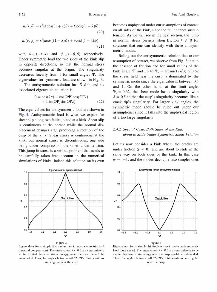
eigenvalues for symmetric load are shown in Fig. 3.

The antisymmetric solution has ~D 6¼ 0, and its

associated eigenvalue equation is:

0 ¼ cosðkpÞ � cosð2WÞcosð2WkÞþ ksinð2WÞsinð2WkÞ: ð22Þ

The eigenvalues for antisymmetric load are shown in

Fig. 4. Antisymmetric load is what we expect for

shear slip along two faults joined at a kink. Shear slip

is continuous at the corner while the normal dis-

placement changes sign producing a rotation of the

cusp of the kink. Shear stress is continuous at the

kink, but normal stress is discontinuous, one side

being under compression, the other under tension.

This jump in stress is a serious problem that needs to

be carefully taken into account in the numerical

simulations of kinks: indeed this solution on its own

becomes unphysical under our assumptions of contact

on all sides of the kink, since the fault cannot sustain

tension. As we will see in the next section, the jump

in normal stress persists when friction f = 0 for

solutions that one can identify with these antisym-

metric modes.

Ruling out the antisymmetric solution due to our

assumption of contact, we observe from Fig. 3 that in

the absence of friction and for small values of the

kink angle W and up to Wl ¼ arcsinð1=ffiffiffi

3pÞ ’ 0:62

the stress field near the cusp is dominated by the

symmetric mode since the eigenvalue is between 0.5

and 1. On the other hand, at the limit angle,

Wl ’ 0:62, the shear mode has a singularity with

k = 0.5 so that the cusp’s singularity becomes like a

crack tip’s singularity. For larger kink angles, the

symmetric mode should be ruled out under our

assumptions, since it falls into the unphysical region

of a too large singularity.

2.4.2 Special Case, Both Sides of the Kink

about to Slide Under Symmetric Shear Friction

Let us now consider a kink where the cracks are

under friction (f = 0), and are about to slide in the

same way on both sides of the kink. In this case

w = -1, and the modes decouple into simpler ones

Figure 3Eigenvalues for a simple frictionless crack under symmetric load

(uniaxial compression). The eigenvalues k \ 0.5 are very unlikely

to be excited because strain energy near the cusp would be

unbounded. Thus, for angles between �0:62\W\0:62 solutions

are singular near the cusp

Figure 4Eigenvalues for a simple frictionless crack under antisymmetric

load (pure shear). The eigenvalues k\ 0.5 are very unlikely to be

excited because strain energy near the cusp would be unbounded.

Thus, for angles between �0:62\W\0:62 solutions are regular

near the cusp

2172 R. Arias et al. Pure Appl. Geophys.

like in the frictionless case of the previous section:

the off-diagonal terms in the matrix of Eq. 52 are

zero so that the eigenvalue equation splits into two.

The first equation is obtained setting ~D ¼ 0 and~C 6¼ 0, and its associated exponent solves the

following equation:

0¼ cosðkpÞþcosð2WÞcosð2WkÞ�ksinð2WÞsinð2WkÞþ f ð1þkÞsinð2WÞcosð2WkÞ; ð23Þ

these are symmetric modes which are very similar

to those computed for a frictionless crack in the

previous section (Eqs. 20 and 21). The main dif-

ference is that now the shear and normal stresses

satisfy the friction law, Eq. 9. For the symmetric

mode slip orientation again corresponds to that of

Fig. 2c. At the cusp the slip directions are in the

same radial direction producing a strong stress

concentration so that the normal and shear stresses

are singular with an exponent k \ 1 for small angles

W. All other properties are the same as for the fric-

tionless case.

The other solution has ~C ¼ 0 and ~D 6¼ 0, and its

associated eigenvalue equation is:

0¼ cosðkpÞ�cosð2WÞcosð2WkÞþksinð2WÞsinð2WkÞ� f ð1þkÞsinð2WÞcosð2WkÞ; ð24Þ

these are antisymmetric modes similar to those of

the frictionless crack discussed above, and we rule

them out due to our assumption of contact. The

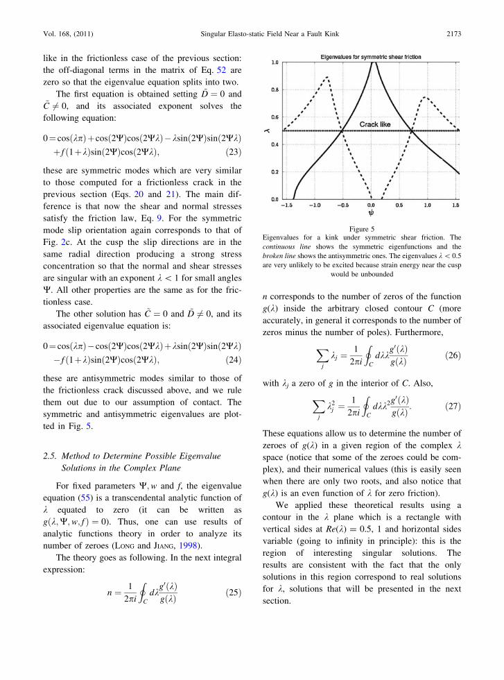
symmetric and antisymmetric eigenvalues are plot-

ted in Fig. 5.

2.5. Method to Determine Possible Eigenvalue

Solutions in the Complex Plane

For fixed parameters W;w and f, the eigenvalue

equation (55) is a transcendental analytic function of

k equated to zero (it can be written as

gðk;W;w; f Þ ¼ 0). Thus, one can use results of

analytic functions theory in order to analyze its

number of zeroes (LONG and JIANG, 1998).

The theory goes as following. In the next integral

expression:

n ¼ 1

2pi

I

C

dkg0ðkÞgðkÞ ð25Þ

n corresponds to the number of zeros of the function

g(k) inside the arbitrary closed contour C (more

accurately, in general it corresponds to the number of

zeros minus the number of poles). Furthermore,

X

j

kj ¼1

2pi

I

C

dkkg0ðkÞgðkÞ ð26Þ

with kj a zero of g in the interior of C. Also,

X

j

k2j ¼

1

2pi

I

C

dkk2g0ðkÞgðkÞ : ð27Þ

These equations allow us to determine the number of

zeroes of g(k) in a given region of the complex kspace (notice that some of the zeroes could be com-

plex), and their numerical values (this is easily seen

when there are only two roots, and also notice that

g(k) is an even function of k for zero friction).

We applied these theoretical results using a

contour in the k plane which is a rectangle with

vertical sides at Re(k) = 0.5, 1 and horizontal sides

variable (going to infinity in principle): this is the

region of interesting singular solutions. The

results are consistent with the fact that the only

solutions in this region correspond to real solutions

for k, solutions that will be presented in the next

section.

Figure 5Eigenvalues for a kink under symmetric shear friction. The

continuous line shows the symmetric eigenfunctions and the

broken line shows the antisymmetric ones. The eigenvalues k \ 0.5

are very unlikely to be excited because strain energy near the cusp

would be unbounded

Vol. 168, (2011) Singular Elasto-static Field Near a Fault Kink 2173

2.6. General Numerical Solutions of Eigenvalue

Equations

We looked for numerical solutions of the eigen-

value equation (55) for the singular solution exponent

k under general frictional conditions near the cusp, and

in the region 0.5 B Re(k) \ 1 (the solutions turned out

to be all real, as explained in the previous section). The

following are plots that show solutions with k real:

they are obtained as contour plots at level zero of a

function gðk;W;w; f Þ with a choice of parameters,

f = 0.4 and varying w (notice that the eigenvalue

equation (55) is written as gðk;W;w; f Þ ¼ 0). Figure 6

shows 2D contour plots with the friction coefficient

f chosen as 0.4,w taken in the four cases as

-1.0, - 0.5, 0.5 and 1.0 respectively, W between 0,

p/2 and k 2 ð0:5; 1:0Þ (the range of interest). Notice

that the plot corresponding to w = -1.0 corresponds

to the special case with both sides about to slide under

symmetric shear that was already presented: in this

case we have shown the roots of the antisymmetric

modes with shaded lines. As w changes in the

following plots (to w = -0.5, 0.5 and 1.0) one sees

a recognizable change of the w = -1 curves, i.e. one

can associate the curves with their symmetric and

antisymmetric origins.

Also, Fig. 7 shows plots of the strength of the

normal stress on both sides of the kink (this is the pre-

factor of the normal stress, there is a radial variation

on top of it), corresponding to the physical roots, k,

found on the previous figures, i.e. with friction

coefficient f chosen as 0.4,w taken in the 4 cases as

1.0 0.5 0.0 0.5 1.00.5

0.6

0.7

0.8

0.9

1.0

1.0 0.5 0.0 0.5 1.00.5

0.6

0.7

0.8

0.9

1.0

1.0 0.5 0.0 0.5 1.00.5

0.6

0.7

0.8

0.9

1.0

1.0 0.5 0.0 0.5 1.00.5

0.6

0.7

0.8

0.9

1.0

Figure 6Roots of the eigenvalue equation for the radial exponent k as a function of the angle W, for four choices of the w coefficient. f = 0.4 and

w = -1.0, -0.5, 0.5 and 1.0 for each successive plot

2174 R. Arias et al. Pure Appl. Geophys.

-1.0, -0.5, 0.5 and 1.0 respectively: these curves

correspond to the curves on Fig. 6 that are or can be

associated with the symmetric modes of w = -1.0.

Indeed with these plots of Fig. 7 one sees that the

normal stress has the same sign on both sides of the

kink for all values of k concerned, meaning that they

correspond to contact modes, i.e. they are consistent

with our assumption of faults under compression. As

w differs from w = -1.0 these modes become of

mixed character, but as far as the sign of the normal

stress on both sides of the kink, it remains the same,

i.e. one could say that the symmetric part prevails on

them.

Notice that the modes that one can associate to the

antisymmetric modes of w = -1 as one changes w,

even though they get mixed character as w changes,

the normal stress differs always in sign along both

sides of the kink meaning that the assumption of

contact cannot be sustained since the faults cannot

sustain tension (in this sense one can say that they

retain mainly an antisymmetric character).

All our numerical calculations were done with

Poisson’s ratio taken as m = 0.3.

Our Fig. 8 are polar plots of rhh and r// for some

allowed solutions, i.e. they reflect the angular vari-

ation of these stresses for specific parameters. We

chose f = 0.4, a = 0.8 (p/2), w = -1.0 for the

upper plot and w = 0.5 for the lower. The angles hand / range from 0 to a and from 0 to b = p - a(another way of thinking about the plot is to take h to

0.6 0.7 0.8 0.9 1.01

2

3

4

5

6

7

0.6 0.7 0.8 0.9 1.01

2

3

4

5

0.6 0.7 0.8 0.9 1.0

1

2

3

4

0.6 0.7 0.8 0.9 1.0

0.5

1.0

1.5

2.0

2.5

3.0

3.5

Figure 7Amplitude of the normal stress along the two branches of the kink (in arbitrary units) as a function of the singular exponent k for four choices

of the w coefficient. f = 0.4 and w = -1.0, -0.5, 0.5 and 1.0 for each successive plot

Vol. 168, (2011) Singular Elasto-static Field Near a Fault Kink 2175

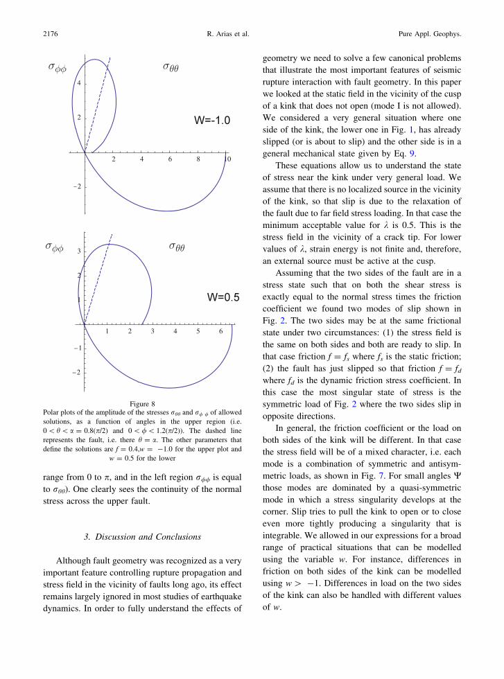
range from 0 to p, and in the left region r// is equal

to rhh). One clearly sees the continuity of the normal

stress across the upper fault.

3. Discussion and Conclusions

Although fault geometry was recognized as a very

important feature controlling rupture propagation and

stress field in the vicinity of faults long ago, its effect

remains largely ignored in most studies of earthquake

dynamics. In order to fully understand the effects of

geometry we need to solve a few canonical problems

that illustrate the most important features of seismic

rupture interaction with fault geometry. In this paper

we looked at the static field in the vicinity of the cusp

of a kink that does not open (mode I is not allowed).

We considered a very general situation where one

side of the kink, the lower one in Fig. 1, has already

slipped (or is about to slip) and the other side is in a

general mechanical state given by Eq. 9.

These equations allow us to understand the state

of stress near the kink under very general load. We

assume that there is no localized source in the vicinity

of the kink, so that slip is due to the relaxation of

the fault due to far field stress loading. In that case the

minimum acceptable value for k is 0.5. This is the

stress field in the vicinity of a crack tip. For lower

values of k, strain energy is not finite and, therefore,

an external source must be active at the cusp.

Assuming that the two sides of the fault are in a

stress state such that on both the shear stress is

exactly equal to the normal stress times the friction

coefficient we found two modes of slip shown in

Fig. 2. The two sides may be at the same frictional

state under two circumstances: (1) the stress field is

the same on both sides and both are ready to slip. In

that case friction f = fs where fs is the static friction;

(2) the fault has just slipped so that friction f = fdwhere fd is the dynamic friction stress coefficient. In

this case the most singular state of stress is the

symmetric load of Fig. 2 where the two sides slip in

opposite directions.

In general, the friction coefficient or the load on

both sides of the kink will be different. In that case

the stress field will be of a mixed character, i.e. each

mode is a combination of symmetric and antisym-

metric loads, as shown in Fig. 7. For small angles Wthose modes are dominated by a quasi-symmetric

mode in which a stress singularity develops at the

corner. Slip tries to pull the kink to open or to close

even more tightly producing a singularity that is

integrable. We allowed in our expressions for a broad

range of practical situations that can be modelled

using the variable w. For instance, differences in

friction on both sides of the kink can be modelled

using w [ -1. Differences in load on the two sides

of the kink can also be handled with different values

of w.

2 4 6 8 10

2

2

4

1 2 3 4 5 6

2

1

1

2

3

Figure 8Polar plots of the amplitude of the stresses rhh and r/ / of allowed

solutions, as a function of angles in the upper region (i.e.

0 \ h\ a = 0.8(p/2) and 0 \/\ 1.2(p/2)). The dashed line

represents the fault, i.e. there h = a. The other parameters that

define the solutions are f = 0.4,w = -1.0 for the upper plot and

w = 0.5 for the lower

2176 R. Arias et al. Pure Appl. Geophys.

Another important issue is that when the stress

field near the corner is strictly antisymmetric, the

stress field is discontinuous at the corner, one side

being under increased tension and the other under

increased compression. This produces a rotation of

the cusp and has an influence on the seismic moment

of the kinked crack. This type of mode, i.e. anti-

symmetric or close to it is ruled out under our model

that assumes contact, since the faults cannot sustain

tension. Thus, this feature will be further studied for a

finite crack with a kink in future work, allowing for

open regions of the faults.

The results presented here provide a general

framework to study the static stress and displacement

fields in the vicinity of a kink on a shear fault. They

can be used to interpret numerical results obtained

using boundary integral or finite element approaches

or, as we expect, they can be used to create particular

elements that better resolve the stress field at the

kink.

Acknowledgments

The authors acknowledge financial support from

project ECOS-CONICYT C06U02.

Appendix

Frictionless Boundary Conditions

We handle separately the boundary condi-

tions, Eqs. 5–7, that are independent of friction

since these allow us to reduce the number of

unknowns. These lead to the following set of

equations:

with

c � ð1þ kÞð1� m2Þ; d � 2k;� � ð1� kÞð1� m2Þ

ð30Þ

Manipulating these equations, and using that

a ? b = p, one gets:

Aa

� �

¼ 1

dsinðkpÞPðbÞ Qða; bÞ

Qðb; aÞ PðaÞ

� �

cC

� �

ð31Þ

with

PðbÞ � m2dcosðð1þ kÞbÞsinðð1� kÞbÞ� csinðð1þ kÞbÞcosðð1� kÞbÞ ð32Þ

Qða; bÞ � m2dcosðð1þ kÞbÞsinðð1� kÞaÞþ csinðð1þ kÞbÞcosðð1� kÞaÞ ð33Þ

0 ¼sinð1þ kÞb m2sinð1� kÞb sinð1þ kÞa m2sinð1� kÞadsinð1þ kÞb �sinð1� kÞb dsinð1þ kÞa �sinð1� kÞadcosð1þ kÞb ccosð1� kÞb �dcosð1þ kÞa �ccosð1� kÞa

0

@

1

A

acAC

0

B

B

@

1

C

C

A

ð28Þ

0 ¼cosð1þ kÞb m2cosð1� kÞb cosð1þ kÞa m2cosð1� kÞadcosð1þ kÞb �cosð1� kÞb dcosð1þ kÞa �cosð1� kÞadsinð1þ kÞb csinð1� kÞb �dsinð1þ kÞa �csinð1� kÞa

0

@

1

A

bdBD

0

B

B

@

1

C

C

A

ð29Þ

Vol. 168, (2011) Singular Elasto-static Field Near a Fault Kink 2177

and

Bb

� �

¼ 1

dsinðkpÞRðbÞ Sða; bÞ

Sðb; aÞ RðaÞ

� �

dD

� �

ð34Þ

with

RðbÞ � m2dsinðð1þ kÞbÞcosðð1� kÞbÞ� ccosðð1þ kÞbÞsinðð1� kÞbÞ ð35Þ

Sða; bÞ � m2dsinðð1þ kÞbÞcosðð1� kÞaÞþ ccosðð1þ kÞbÞsinðð1� kÞaÞ ð36Þ

Thus, one has obtained expressions for A =

A(c, C), a = a(c, C), B = B(d, D) and b = b(d, D).

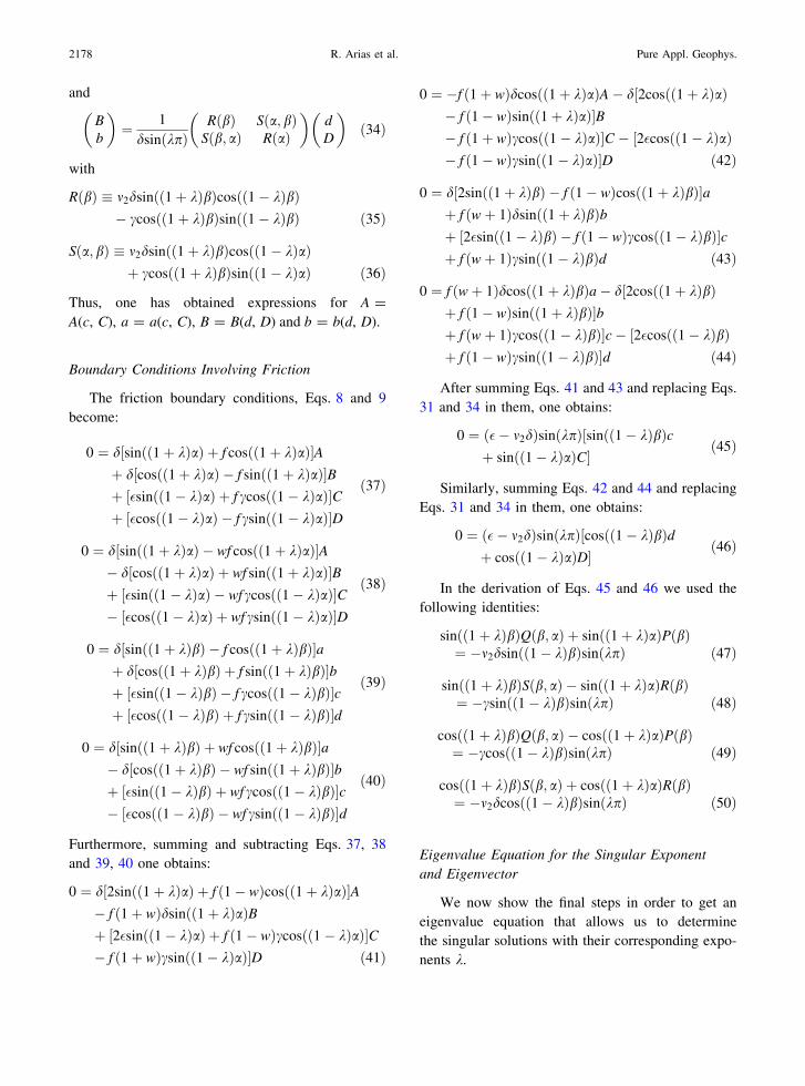
Boundary Conditions Involving Friction

The friction boundary conditions, Eqs. 8 and 9

become:

0 ¼ d½sinðð1þ kÞaÞ þ f cosðð1þ kÞaÞ�Aþ d½cosðð1þ kÞaÞ � f sinðð1þ kÞaÞ�Bþ ½�sinðð1� kÞaÞ þ f ccosðð1� kÞaÞ�Cþ ½�cosðð1� kÞaÞ � f csinðð1� kÞaÞ�D

ð37Þ

0 ¼ d½sinðð1þ kÞaÞ � wf cosðð1þ kÞaÞ�A� d½cosðð1þ kÞaÞ þ wf sinðð1þ kÞaÞ�Bþ ½�sinðð1� kÞaÞ � wf ccosðð1� kÞaÞ�C� ½�cosðð1� kÞaÞ þ wf csinðð1� kÞaÞ�D

ð38Þ

0 ¼ d½sinðð1þ kÞbÞ � f cosðð1þ kÞbÞ�aþ d½cosðð1þ kÞbÞ þ f sinðð1þ kÞbÞ�bþ ½�sinðð1� kÞbÞ � f ccosðð1� kÞbÞ�cþ ½�cosðð1� kÞbÞ þ f csinðð1� kÞbÞ�d

ð39Þ

0 ¼ d½sinðð1þ kÞbÞ þ wf cosðð1þ kÞbÞ�a� d½cosðð1þ kÞbÞ � wf sinðð1þ kÞbÞ�bþ ½�sinðð1� kÞbÞ þ wf ccosðð1� kÞbÞ�c� ½�cosðð1� kÞbÞ � wf csinðð1� kÞbÞ�d

ð40Þ

Furthermore, summing and subtracting Eqs. 37, 38

and 39, 40 one obtains:

0 ¼ d½2sinðð1þ kÞaÞ þ f ð1� wÞcosðð1þ kÞaÞ�A� f ð1þ wÞdsinðð1þ kÞaÞBþ ½2�sinðð1� kÞaÞ þ f ð1� wÞccosðð1� kÞaÞ�C� f ð1þ wÞcsinðð1� kÞaÞ�D ð41Þ

0 ¼ �f ð1þ wÞdcosðð1þ kÞaÞA� d½2cosðð1þ kÞaÞ� f ð1� wÞsinðð1þ kÞaÞ�B� f ð1þ wÞccosðð1� kÞaÞ�C � ½2�cosðð1� kÞaÞ� f ð1� wÞcsinðð1� kÞaÞ�D ð42Þ

0 ¼ d½2sinðð1þ kÞbÞ � f ð1� wÞcosðð1þ kÞbÞ�aþ f ðwþ 1Þdsinðð1þ kÞbÞbþ ½2�sinðð1� kÞbÞ � f ð1� wÞccosðð1� kÞbÞ�cþ f ðwþ 1Þcsinðð1� kÞbÞd ð43Þ

0 ¼ f ðwþ 1Þdcosðð1þ kÞbÞa� d½2cosðð1þ kÞbÞþ f ð1� wÞsinðð1þ kÞbÞ�bþ f ðwþ 1Þccosðð1� kÞbÞ�c� ½2�cosðð1� kÞbÞþ f ð1� wÞcsinðð1� kÞbÞ�d ð44Þ

After summing Eqs. 41 and 43 and replacing Eqs.

31 and 34 in them, one obtains:

0 ¼ ð�� m2dÞsinðkpÞ½sinðð1� kÞbÞcþ sinðð1� kÞaÞC�

ð45Þ

Similarly, summing Eqs. 42 and 44 and replacing

Eqs. 31 and 34 in them, one obtains:

0 ¼ ð�� m2dÞsinðkpÞ½cosðð1� kÞbÞdþ cosðð1� kÞaÞD�

ð46Þ

In the derivation of Eqs. 45 and 46 we used the

following identities:

sinðð1þ kÞbÞQðb; aÞ þ sinðð1þ kÞaÞPðbÞ¼ �m2dsinðð1� kÞbÞsinðkpÞ ð47Þ

sinðð1þ kÞbÞSðb; aÞ � sinðð1þ kÞaÞRðbÞ¼ �csinðð1� kÞbÞsinðkpÞ ð48Þ

cosðð1þ kÞbÞQðb; aÞ � cosðð1þ kÞaÞPðbÞ¼ �ccosðð1� kÞbÞsinðkpÞ ð49Þ

cosðð1þ kÞbÞSðb; aÞ þ cosðð1þ kÞaÞRðbÞ¼ �m2dcosðð1� kÞbÞsinðkpÞ ð50Þ

Eigenvalue Equation for the Singular Exponent

and Eigenvector

We now show the final steps in order to get an

eigenvalue equation that allows us to determine

the singular solutions with their corresponding expo-

nents k.

2178 R. Arias et al. Pure Appl. Geophys.

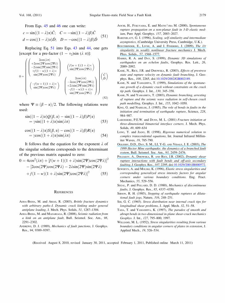
From Eqs. 45 and 46 one can write:

c¼ sinðð1� kÞaÞ ~C; C ¼�sinðð1� kÞbÞ ~C

d ¼ cosðð1� kÞaÞ ~D; D¼�cosðð1� kÞbÞ ~Dð51Þ

Replacing Eq. 51 into Eqs. 43 and 44, one gets

[except for a pre-factor (1 - m2)sin (k p)]:

0 ¼

2cosðkpÞþ2cosð2WÞcosð2WkÞ�2ksinð2WÞsinð2WkÞþf ð1� wÞð1þ kÞ�sinð2WÞcosð2WkÞ

0

B

B

B

B

@

1

C

C

C

C

A

f ðwþ 1Þð1þ kÞ�sinð2WÞcosð2WkÞ

� �

�f ðwþ 1Þð1þ kÞ�sinð2WÞcosð2WkÞ

� �

2cosðkpÞ�2cosð2WÞcosð2WkÞþ2ksinð2WÞsinð2WkÞ�f ð1� wÞð1þ kÞ�sinð2WÞcosð2WkÞ

0

B

B

B

B

@

1

C

C

C

C

A

0

B

B

B

B

B

B

B

B

B

B

B

B

B

B

@

1

C

C

C

C

C

C

C

C

C

C

C

C

C

C

A

~C~D

� �

ð52Þ

where W � ðb� aÞ=2. The following relations were

used:

sinðð1� kÞaÞQðb; aÞ � sinðð1� kÞbÞPðaÞ¼ csinðð1þ kÞaÞsinðkpÞ ð53Þ

cosðð1� kÞaÞSðb; aÞ � cosðð1� kÞbÞRðaÞ¼ ccosðð1þ kÞaÞsinðkpÞ ð54Þ

It follows that the equation for the exponent k of

the singular solutions corresponds to the determinant

of the previous matrix equated to zero:

0 ¼ 4cos2ðkpÞ þ ½f ðwþ 1Þð1þ kÞsinð2WÞcosð2WkÞ�2

� ½2cosð2WÞcosð2WkÞ � 2ksinð2WÞsinð2WkÞþ f ð1� wÞð1þ kÞsinð2WÞcosð2WkÞ�2 ð55Þ

REFERENCES

ADDA-BEDIA, M. and ARIAS, R. (2003), Brittle fracture dynamics

with arbitrary paths–I. Dynamic crack kinking under general

antiplane loading, J. Mech. Phys. Solids, 51, 1287–1304.

ADDA-BEDIA, M. and MADARIAGA, R. (2008), Seismic radiation from

a kink on an antiplane fault, Bull. Seismol. Soc. Am., 98,

2291–2302.

ANDREWS, D. J. (1989), Mechanics of fault junctions, J. Geophys.

Res., 94, 9389–9397.

AOCHI, H., FUKUYAMA, E. and MATSU’URA M. (2000), Spontaneous

rupture propagation on a non-planar fault in 3-D elastic med-

ium, Pure Appl. Geophys. 157, 2003–2027.

BARENBLATT, G. I. (1996), Scaling, self-similarity and intermediate

asymptotics, (Cambridge University Press, Cambridge, U.K.).

BOUCHBINDER, E., LIVNE, A. and J. FINEBERG, J. (2009), The 1/r

singularity in weakly nonlinear fracture mechanics J. Mech.

Phys. Solids., 57, 1568–1577.

HARRIS, R. A. and DAY, S. (1999), Dynamic 3D simulations of

earthquakes on an echelon faults, Geophys. Res. Lett., 26,

2089–2092.

KAME, N., RICE, J.R. and DMOWSKA, R. (2003), Effects of prestress

state and rupture velocity on dynamic fault branching, J. Geo-

phys. Res., 108, 2265, doi:10.1029/2002JGB002189.

KAME, N. and YAMASHITA, T. (1999), Simulations of the spontane-

ous growth of a dynamic crack without constraints on the crack

tip path. Geophys. J. Int., 130, 345–358.

KAME, N. and YAMASHITA, T. (2003), Dynamic branching, arresting

of rupture and the seismic wave radiation in self-chosen crack

path modelling, Geophys. J. Int., 155, 1042–1050.

KING, G. and NABELEK, J. (1985), The role of bends in faults in the

initiation and termination of earthquake rupture, Science, 228,

984–987.

LABOSSIERE, P.E.W. and DUNN, M. L. (2001) Fracture initiation at

three-dimensional bimaterial interface corners. J. Mech. Phys.

Solids, 49, 609–634

LONG, Y. and JIANG, H. (1998), Rigorous numerical solution to

complex transcendental equations, Int. Journal Infrared Millim-

iter Waves, 19, 785-790.

OGLESBY, D.D., DAY, S. M., LI, Y-G. AND VIDALE, J. E. (2003), The

1999 Hector Mine earthquake: the dynamics of a branched fault

system, Bull. Seismol. Soc. Am., 93, 2459–2476.

POLIAKOV, A., DMOWSKA, R. AND RICE, J.R. (2002), Dynamic shear

rupture interactions with fault bends and off-axis secondary

faulting, J. Geophys. Res., 107, 2295, doi:10.1029/2001JB000572.

SEWERYN, A. and MOLSKI, K. (1996), Elastic stress singularities and

corresponding generalized stress intensity factors for angular

corners under various boundary conditions. Eng. Fract.

Mechanics, 55, 529–556.

SEGAL, P. and POLLARD, D. D. (1980), Mechanics of discontinuous

faults, J. Geophys. Res., 85, 4337–4350.

SIBSON, R. H. (1985), Stopping of earthquake ruptures at dilata-

tional fault jogs, Nature, 316, 248–251.

SIH, G. C. (1965). Stress distribution near internal crack tips for

longitudinal shear problems, J. Appl. Mech. 32, 51–58.

TADA, T. and YAMASHITA, K. (1997), The paradox of smooth and

abrupt bends in two-dimensional in-plane shear-crack mechanics

Geophys. J. Int., 127, 795–800, 1997.

WILLIAMS, M. L. (1952), Stress singularities resulting from various

boundary conditions in angular corners of plates in extension, J.

Applied Mech., 19, 526–534.

(Received August 8, 2010, revised January 30, 2011, accepted February 1, 2011, Published online March 11, 2011)

Vol. 168, (2011) Singular Elasto-static Field Near a Fault Kink 2179