General solution procedures in elasto/viscoplasticity

Giulio Alfano, Fabio De Angelis, Luciano Rosati *

Dipartimento di Scienza delle Costruzioni, Facolt�a di Ingegneria, Universit�a di Napoli ``Federico II'', Via Claudio 21,

80125 Napoli, Italy

Received 3 March 2000; received in revised form 28 July 2000

Abstract

Constitutive relations and numerical integration algorithms for elasto/viscoplastic problems are investigated. A fully implicit in-

tegration scheme is adopted and the relevant expression of the consistent tangent operator for yield criteria and ¯ow functions of

arbitrary type is derived by suitably generalizing the approach exploited for rate-independent plasticity. This is achieved by replacing

the consistency condition of plasticity with a relation between the viscoplastic consistency parameter and the ¯ow function of the

constitutive model in use. The methodology adopted simpli®es alternative procedures for the evaluation of consistent tangent oper-

ators which necessitate the inversion of a viscoplastic compliance operator. The general expression of the consistent tangent operator is

then specialized to the von Mises yield criterion endowed with commonly adopted viscoplastic constitutive models. Numerical ex-

amples are ®nally presented. Ó 2001 Elsevier Science B.V. All rights reserved.

Keywords: Elasto/viscoplasticity; Numerical solution procedures; Finite elements

1. Introduction

The subject of the continuum problem of evolution in elasto/viscoplasticity has nowadays accomplished

a deep mathematical understanding throughout the works of, among others, Hill [12], Koiter [18], Mandel

[24], Duvaut and Lions [7], Germain et al. [9], Naghdi and Murch [26], Perzyna [32,33], Moreau [25],

Nguyen [28], Rice [35,36], Simo [42], Suquet [46] and Temam [50]. A comprehensive account can be found,

e.g. in [8,21,45].

In this paper, reference will be made to the class of material models for which viscous phenomena take

place beyond the elastic range. It is customary in the literature [33,45] to address them with the denomi-

nation elasto/viscoplasticity as opposite to the alternative expression, elasto-viscoplasticity, used to denote

material behaviours in which viscous e�ects play an e�ective role also in the elastic regime.

In the last two decades, elasto/viscoplasticity has attained a signi®cant progress not only in the de®nition

of the appropriate theoretical framework but also in the computational treatment of the relevant boundary

value problem.

Numerical algorithms for the constitutive problem have been mainly derived from plasticity and rely on

the classical operator split methodology based on an elastic prediction and a plastic correction phase. In

this respect we remind that integration algorithms in plasticity have been introduced by Wilkins [52] in the

form of a radial return algorithm with reference to the Mises criterion, and successively extended by Krieg

and Key [20] to the case of isotropic and kinematic hardening. Di�erent formulation of predictor±corrector

www.elsevier.com/locate/cma

Comput. Methods Appl. Mech. Engrg. 190 !2001) 5123±5147

*Corresponding author.

E-mail address: rosati@unina.it !L. Rosati).

0045-7825/01/$ - see front matter Ó 2001 Elsevier Science B.V. All rights reserved.

PII: S 0 0 4 5 - 7 8 2 5 ! 0 0 ) 0 0 3 7 0 - 4

algorithms has been then proposed by Krieg and Krieg [19] and subsequently extended to a multitude of

constitutive models of inelastic behaviour, see [5] for a survey account.

The numerical integration of the rate-dependent !viscoplastic) problem is not trivial. Zienkiewicz and

Cormeau [54] developed an algorithm for quasi-static elasto/viscoplasticity problems, which gives time step

restrictions for the Euler forward di�erence method. Hughes and Taylor [15] then proposed the application

of implicit methods to quasi-static elasto/viscoplasticity which requires the inversion of a compliance matrix.

Pierce et al. [31] proposed a one-step forward gradient time integration scheme which leads to a tangent

sti�ness type method for rate-dependent solids. In a review article, Szabo [48] compared di�erent time ite-

gration schemes and proposed a new method for the calculation of the e�ective viscoplastic strain increment.

Peric [30] used a perturbation method for the solution of sti� equations arising in low-rate-sensitive

materials and proposed a new constitutive model of viscoplastic behaviour. Chaboche and Cailletaud [4]

analysed models including non-linear hardening behaviour and showed alternative integration procedures

especially designed for material models in which the ratchetting !accumulated strain) or the cyclic stress

relaxation plays a signi®cant role.

The necessity to take into account the numerical integration procedure into the evaluation of the tangent

operator has been ®rst outlined by Nagtegaal [27]. For this reason, Simo and Taylor [44] showed the ne-

cessity of replacing the ``continuum'' tangent operator with the consistent tangent one, since the latter

restores the quadratic rate of convergence typical of iterative solution schemes based on Newton's method.

The importance of the consistent tangent operator for viscoplastic models was subsequently emphasized by

Ju [16], who pointed out that ``continuum tangents do not even exist for viscoplasticity''.

In the present paper, the evolutive process of rate-dependent problems and its numerical implementation

are addressed within the framework of an internal variable theory [24,36], by exploiting the model of the

generalized standard material !GSM) introduced by Halphen and Nguyen [11]. Remarkably, the GSM

allows one to handle the elasto/viscoplastic problems with hardening by adopting the same formal rules of

the elastic-perfectly viscoplastic model provided that a suitable de®nition of the internal variables and of

the yield function is assumed.

In particular we refer to the classical treatment of elasto/viscoplasticity of the Perzyna type [33,34] and to

the modi®cation recently proposed by Peric [30]. The interpretation of the rate-dependent phenomenon as a

penalty regularization of the rate-independent one [53] is applied, by specializing to the present context

concepts and properties ®rst introduced by Moreau [25] and recently enlightened by Simo et al. [42,43].

The solution of the viscoplastic constitutive problem is pursued by following the same lines of reasoning

used for rate-independent models. Speci®cally, the evolution of the viscoplastic multiplier is related to the

¯ow function depending upon the adopted viscoplastic constitutive model, thus developing the method-

ology brie¯y alluded to by Simo in [40]. Such an approach is further enhanced in this paper by showing how

it can be combined with the procedure outlined in [2] for deriving closed form expressions of the consistent

tangent operator for yield functions of arbitrary type.

The resulting expression of the consistent tangent operator is quite general and it can be specialized to

di�erent yield criteria. Moreover, several viscoplastic constitutive models can be addressed in a straight-

forward manner by suitably de®ning the relevant ¯ow function. As an example we explicitly derive the

expression of the tangent operator for the von Mises yield criterion and Perzyna-like viscoplastic models. In

particular, it is shown that the resulting expression of the general form of the consistent tangent operator

coincides with the one that Ju [16] derived, in the absence of hardening, by following a procedure specif-

ically tailored for J2 models and requiring the inversion of a viscoplastic compliance operator.

Numerical computations are reported to validate the robustness of the integration procedure. Fur-

thermore, connections and relations between the viscoplastic problem !rate-dependent) and the elasto-

plastic problem !rate-independent) are also illustrated.

2. Continuum problem of evolution

The continuum problem of evolution is detailed by making use of the GSM model [11], which allows one

to treat the evolutive problem with hardening in a compact form by introducing generalized variables which

5124 G. Alfano et al. / Comput. Methods Appl. Mech. Engrg. 190 !2001) 5123±5147

collect state and internal variables [24,36]. After introducing some basic notations, the generalized standard

material model is brie¯y reviewed and the evolutive laws for the state variables and the internal variables

are illustrated.

Let X � Rn, 16 n6 3, be the reference con®guration of an elastic/viscoplastic body B with smooth

boundary oX, closure �X�def

X [ oX and particles labelled x 2 X. The time interval of interest, during which

the analysis of the structural model is carried out, is denoted by T � R�, while V is the linear space of

displacements, D the strain space and S is the dual stress space. We indicate with

u : X�T ! V

the displacement ®eld, and with

r : X�T ! S

the stress ®eld. The hypothesis of small strains is made and, accordingly, the strain ®eld

e : X�T ! D

is de®ned as e � rs�u�, where rs is the symmetric part of the gradient. Furthermore, a quasi-static for-

mulation is assumed.

The hypothesis of small strains allows to additively split the total strain e into the elastic and inelastic

parts, respectively denoted by ee and ein:

ee � eÿ ein: �2:1�

In the sequel, the inelastic strain will be denoted as plastic strain p for the rate-independent material

model and viscoplastic strain evp for the rate-dependent behaviour.

As originally proposed by Naghdi and Murch [26], we assume that the viscous e�ects are exhibited

beyond the elastic range. This class of material behaviour is often denoted in the literature as rate sensitive

[33,34].

The one-to-one relation E between the elastic strain ee 2 D and the stress r 2 S, as well as its inverse Eÿ1,

r � E�ee�; ee � Eÿ1�r� �2:2�

de®ne the constitutive elastic relation. It ful®ls the property of stability, which is equivalent to the strict

monotonocity of the graph of the operator E, or to the property that the derivative dE is positive de®nite.

Another important property of the elastic constitutive relation is its conservativity which is related to the

non-dissipativity of the elastic relation. These properties lead to the existence of a strictly convex potential

W : D ! R of the operator E, differentiable since E is one-to-one, so that

E�ee� � dW�ee� 8ee 2 D:

The potential W�ee� expresses the elastic energy per unit volume, while the potential W��r�, conjugate of

W�ee�, represents the complementary elastic energy.

Assuming linear elasticity, the sti�ness operator Eÿ1 and the compliance operator Eÿ1 will be denoted by

E and Eÿ1. In this case, relations !2.2) specialize to

r � Eee; ee � Eÿ1r: �2:3�

The conservativity property of the elastic operator, that is the existence of the potential W, results in the

major symmetry of the operators E and Eÿ1.

The elastic energy W�ee� and the complementary elastic energy W��r� also specialize to the quadratic

forms

W�ee� �1

2hEee; ei; W

��r� �1

2hr;Eÿ1ri

which are positive de®nite due to the above-mentioned stability property. Herein the symbol h�; �i has beenused to denote a non-degenerate bilinear form acting on dual spaces.

G. Alfano et al. / Comput. Methods Appl. Mech. Engrg. 190 !2001) 5123±5147 5125

The closed convex elastic domain in the stress space is expressed as

C �def

r 2 S : f �r�f 6 0g; �2:4�

where f �r� denotes the yield function whose zero level set provides the boundary of the elastic domain

oC �def

fr 2 S : f �r� � 0g:

Let us now introduce a kinematic internal variable akin and a static one vkin to model kinematic hard-

ening. They have tensorial nature and belong to the dual spaces X and X0, respectively. Analogously,

isotropic hardening is modelled by introducing the scalar variables aiso 2 R and viso 2 R. To simplify the

notation it is convenient to group internal variables as follows:

a �akinaiso

� �

; v �vkinviso

� �

; �2:5�

where a 2 X � R and v 2 X0 � R.

Further, we introduce the function H : X � R ! R which represents the hardening potential and the

function H� : X 0 � R ! R, conjugate of H, representing the complementary hardening potential. The

following equivalent relations

v � dH�a� ") a � dH��v� �2:6�

are in turn equivalent to the relation in the Legendre form [37]

H�a� �H��v� � v � a �2:7�

and hold true for conjugate pairs fv; ag.The following uncoupled forms are generally assumed for the hardening and the complementary

hardening potentials, which separately take into account isotropic and kinematic hardening:

H�a� � Hkin�akin� �Hiso�aiso�;

H��v� � H

�kin�vkin� �H

�iso�viso�:

In case of linear hardening static and kinematic internal variables are related by

v � Ha ") a � Hÿ1v; �2:8�

where H denotes the hardening matrix

H �Hkin 0

0T Hiso:

� �

:

Therefore, the hardening potential and the complementary hardening potential are expressed as quadratic

forms and assume the expressions

H�a� �1

2Hkinakin � akin �

1

2Hisoa

2iso

H��v� �

1

2vkin �H

ÿ1kinvkin �

1

2Hÿ1

iso v2iso;

from which we infer vkin � Hkinakin and viso � Hisoaiso.

2.1. The generalized standard material !GSM)

A wide class of inelastic behaviours can be dealt with in a uni®ed manner by resorting to the GSM model

proposed by Halphen and Nguyen [11]. To this end, strains and kinematic internal variables, as well as the

corresponding dual ones, are collected in suitably de®ned generalized variables for which the same formal

rules of the basic variables do apply. With reference to elasto/viscoplasticity with hardening we de®ne

5126 G. Alfano et al. / Comput. Methods Appl. Mech. Engrg. 190 !2001) 5123±5147

~e �e

o

� �

; ~ee �ee

a

� �

; ~p �p

ÿa

� �

; ~evp �evp

ÿa

� �

; ~r �r

v

� �

;

where the generalized kinematic variables belong to the product space ~D � D� X � R and ~r belongs to~S � S � X

0 � R. Notice that the additive decomposition !2.1) of the strain is carried over to the generalized

counterparts

~e � ~ee � ~evp: �2:9�

Further, for typographic convenience, the equivalent notation ~e � �e; o� and ~r � �r; v� will be used in the

sequel.

The duality product between generalized variables is de®ned as the one induced by the duality products

between the corresponding elements of D and S and between the corresponding elements of X � R and

X0 � R:

h~r;~ei � hr; ei; h~r;~eei � hr; eei � hv; ai;

h~r; ~pi � hr; pi ÿ hv; ai; h~r;~evpi � hr; evpi ÿ hv; ai;

where, for simplicity, the same symbol h�; �i has been used to indicate duality products de®ned on di�erent

pairs of vector spaces.

The plastic consistency condition is de®ned by imposing that the generalized stress ~r is constrained to the

generalized convex elastic domain ~C � ~S de®ned as

~C �def

~r 2 ~S : ~f �~r�n

6 0 ") �r; v� 2 S � X0 � R : f �r; v�6 0

o

; �2:10�

where ~f : ~S ! R denotes the yield function expressed in terms of the generalized stress. In particular, we

shall make reference to a fairly general form of the yield function

f �r; vkin; viso� ��f �rÿ vkin� ÿ viso ÿ �ry; �2:11�

where �f is a positively homogeneous convex function and �ry represents a quantity related to the yield limit

of the virgin material.

With this position at hand viscoplasticity with hardening may be formally dealt with similarly to perfect

plasticity. Therefore, for the de®nition of the ¯ow law, it is su�cient to de®ne the internal variables and the

yield function in terms of the generalized variables [38].

2.2. Viscoplastic constitutive model

Viscoplasticity may be usefully considered [53] as a regularization process of the plasticity case !see e.g.

[42]).

Consequently, constitutive equations in viscoplasticity are herein presented as optimality conditions of a

properly regularized function representing the maximum viscoplastic dissipation.

In plasticity, the principle of maximum plastic dissipation [12]

D� _~p� � sup~s2 ~C

fh~s; _~pig �2:12�

embodies the essential structure of constitutive behaviour [13,35] and may be transformed into an equiv-

alent minimum principle

inf~s2 ~C

fÿh~s; _~pig: �2:13�

In viscoplasticity this constrained minimum problem is transformed into an unconstrained problem, by

adding to the objective function to be minimized a penalty function g� : R ! R� of the constraint ~f �~r�6 0

G. Alfano et al. / Comput. Methods Appl. Mech. Engrg. 190 !2001) 5123±5147 5127

ampli®ed by a penalty parameter 1=g. By modifying the parameter g, the following set of problems is

obtained

inf~s2~S

~Lvpg �~s�; �2:14�

where the regularized function ~Lvpg �~s� is expressed by

~Lvpg �~s� �

defÿ h~s; _~evpi �

1

gg�� ~f �~s��; �2:15�

and the parameter g 2 �0;�1� represents a viscosity coe�cient. Here, ~s � �s; q� indicates the generic

generalized stress state, while ~r � �r; v� denotes the value at the solution.

The penalty function g� of the constraint ~f �~r�6 0 has to meet particular conditions [23]: !a) it has to be

of class C1; !b) it has to be non-negative, de®ned in R and such that g��x� � 0 if and only if x6 0.

When these conditions are ful®lled, problem !2.14) is said to be a penalty regularization of the con-

strained plastic problem and the solution ~rg of the regularized problem tends to the solution ~r of the

constrained problem for g ! 0 [23].

The viscoplastic dissipation may therefore be expressed in the regularized form

D�_~evp� � sup~s2~S

h~s; _~evpi

�

ÿ1

gg�� ~f �~s��

�

: �2:16�

By properly choosing the penalty function, di�erent specializations of the viscoplastic constitutive relation

are obtained. For example, by assuming the penalty function g� in the form

g� �def

12x2 for xP 0;

0 for x6 0;

�

the derivative is given by

dg��x�

d�x��

x for xP 0

0 for x6 0

� �

�def

hxi;

where the McAuley brackets are de®ned as hxi � �x� jxj�=2.Therefore, the optimality conditions of the unconstrained problem yield

0 2 o~s~Lvp

g �~s�h i

�~r�") _~evp 2

1

gh ~f �~r�io ~f �~r�; �2:17�

where o denotes the subdi�erential operator [14,37]. In components, the previous relation becomes

0 2 os~Lvp

g �s; q�h i

�r;v�

0 2 oq~Lvp

g �s; q�h i

�r;v�

8

>

<

>

:

")_evp 2 1

ghf �r; v�iorf �r; v�;

ÿ _a 2 1ghf �r; v�iovf �r; v�:

!

�2:18�

They, respectively, represent the normality law and the internal variable evolutive law for the Perzyna

viscoplastic constitutive model [32], with linear viscous e�ects, endowed with hardening. In the general case,

by setting

U�x� �dg��x�

dx;

we get

_evp 2 1ghU�f �r; v��iorf �r; v�;

ÿ _a 2 1ghU�f �r; v��iovf �r; v�:

!

�2:19�

Typical expressions of the ¯ow function U are reported, for instance, in [33,45].

5128 G. Alfano et al. / Comput. Methods Appl. Mech. Engrg. 190 !2001) 5123±5147

The viscoplastic constitutive model has here been presented in subdi�erential form [14,37]. The multi-

valuedness of the subdi�erential operator o ~f �~r� allows for a proper use of this form of constitutive relations

in the general case of non-smooth viscoplasticity. This case has been considered for example by Simo et al.

[43], even though the viscoplastic ¯ow law is still expressed in Koiter's form [17,18]. On the contrary, in this

paper a more general formulation is adopted in the general context of subdi�erential calculus and multi-

valued operators which allows one to properly treat singularities characteristic in non-smooth problems.

For a generalized formulation of constitutive and structural models in non-smooth elasto/viscoplasticity

within the context of subdi�erential calculus and multivalued operators the reader may refer to De Angelis

[6].

3. Discrete formulation and numerical solution

The general framework outlined in the previous section is here applied to a fairly general class of

viscoplastic constitutive models for which numerical integration procedures are detailed.

3.1. Time discretization of the evolutive laws

The solution of the constitutive problem in elasto/viscoplasticity is carried out by subdividing the time

interval of interest T � R� into a ®nite number of time steps. The unknown functions are substituted by

the algorithmic values assumed at the beginning and at the end of the time steps so that the original

problem is reduced to subsequent solutions of ®nite step problems.

In the generic time step tn ! tn�1, the values of the state variables at time tn are known from the previous

analysis while the values at time tn�1 have to be determined. We will indicate with ���n the known value of

the generic variable ��� at time tn and with ���n�1 the unknown value at time tn�1.

From a computational standpoint the problem of evolution may be regarded as strain driven in the

following sense. At time tn the total and viscoplastic strain ®elds and the kinematic internal variable are

considered to be known, that is

en; evpn ; an

�

given data at time tn: �3:1�

The elastic strain tensor, the stress tensor and the static internal variable can then be computed via

Eqs. !2.1), !2.3)1, !2.8)1 and !2.19). Assuming the incremental displacement ®eld un�1 ÿ un to be given, the

basic problem is then to update the ®elds !3.1) to tn�1 in a manner consistent with the constitutive equations

governing the continuum viscoplastic problem of evolution.

The algorithmic value of a generic variable x within the time step is evaluated as !see e.g. [29])

xn�b � xn � b�xn�1 ÿ xn�; b 2 �0; 1�:

This family of integration algorithms includes well-known schemes. In particular, for b � 0, the explicit

integration scheme !often referred to in the literature as forward Euler) is obtained. For b � 1=2 the mid-

point integration scheme is recovered. For b � 1 the fully implicit or backward Euler integration scheme is

attained.

3.2. Discrete form of the evolutive laws and integration algorithm

As noted in [29], a mid-point rule !b � 1=2) yields second-order accuracy, however this holds only for

small strain increments. Conversely, the fully implicit scheme ensures !®rst-order) accuracy and stability

also for large strain increments [15,19,29,39,41]. For this reason we shall adopt a backward Euler scheme

for the time integration of the constitutive model.

Consequently, the continuum problem of evolution addressed in Section 2 may be written in the fol-

lowing discrete form:

G. Alfano et al. / Comput. Methods Appl. Mech. Engrg. 190 !2001) 5123±5147 5129

en�1 � en �rs�Du�

rn�1 � E�en�1 ÿ evpn�1�

vn�1 � vn �H�an�1 ÿ an�

evpn�1 � evpn �

Dt

ghU�f �rn�1; vn�1��i

of �r; v�

or

� �

�rn�1;vn�1�

an�1 � an ÿDt

ghU�f �rn�1; vn�1��i

of �r; v�

ov

� �

�rn�1;vn�1�

;

�3:2�

where Dt � tn�1 ÿ tn and the last two equations stem from !2.19).

In the sequel, the treatment is specialized to the case of J2 viscoplasticity obeying the von Mises criterion.

The yield function is thus expressed in the form

f �r; v� � kdev�rÿ vkin�k ÿ viso � kdev�rÿ vkin�k ÿ R;

where

R � viso �

���

2

3

r

dHiso�aiso�

represents the radius of the yield surface in the deviatoric plane. Due to isotropic hardening it evolves

during the viscoplastic process as a function of the equivalent viscoplastic strain

�evp �

Z t

0

���

2

3

r

k_evpkdt;

which is assumed to represent the kinematic internal variable, that is aiso �def

�evp.

Assuming linear isotropic hardening we can write

dHiso�aiso� � ry � Hiso�evp;

where ry is the uniaxial yield stress of the virgin material and Hiso is the isotropic hardening modulus.

The von Mises criterion may thus be expressed in the form

f �r; v� � knk ÿ

���

2

3

r

�ry � Hiso�evp�; �3:3�

where n � dev�rÿ vkin�.Resulting

on

or� ÿ

on

ovkin� Iÿ

1

31 1 � Idev; �3:4�

where I and 1 are in turn the rank-four and rank-two identity tensors, we get

drf �of �r; v�

or� ÿ

of �r; v�

ovkin�

n

knk� n: �3:5�

We shall also assume

Hkin �2

3HkinI; �3:6�

where Hkin is the kinematic hardening modulus, so as to recover the classical kinematic hardening law

vkin �2

3Hkinakin;

to avoid clutter of symbols we will denote in the sequel the back stress vkin as b.

5130 G. Alfano et al. / Comput. Methods Appl. Mech. Engrg. 190 !2001) 5123±5147

Recalling de®nition !2.5)1 of a, the ¯ow law and the evolutive laws for the internal variables may be

expressed in the discrete form

evpn�1 ÿ evpn �

Dt

ghU�f �rn�1; bn�1;Rn�1��inn�1;

�akin�n�1 ÿ �akin�n �Dt

ghU�f �rn�1; bn�1;Rn�1��inn�1; �3:7�

�evpn�1 ÿ �evpn �

���

2

3

r

Dt

ghU�f �rn�1; bn�1;Rn�1��i;

where nn�1 � �drf �n�1.

The ®rst two equations of the previous set show that, being zero the values of evp and akin at the be-

ginning of the evolution problem, we can set akin � evp in the sequel, ruling out Eq. !3.7)2.

The viscoplastic problem may be expressed in a form analogous to the inviscid one by introducing a time

step dependent viscoplastic multiplier [41,42] which assumes the expression

cvp �Dt

ghU�f �rn�1; bn�1;Rn�1��i �

Dt

ghU�fn�1�i: �3:8�

In conclusion, the specialization of the evolutive constitutive equations to the von Mises model may then be

written as follows:

rn�1 � E�en�1 ÿ evpn�1�;

evpn�1 � evpn � cvpnn�1;

bn�1 � bn �2

3Hkinc

vpnn�1;

�evpn�1 � �evpn �

���

2

3

r

cvp;

Rn�1 � Rn �2

3Hisoc

vp;

�3:9�

where

Rn �

���

2

3

r

ry

�

� Hiso�evpn

�

:

Assuming linear elasticity, the elastic operator E is supplied by

E � k�1 1� � 2G I

�

ÿ1

3�1 1�

�

; �3:10�

where k and G are the bulk and shear moduli, respectively.

The numerical solution of the viscoplastic problem may be pursued according to the standard operator

split methodology which results in the following algorithmic procedure.

Let us indicate by e � dev e the strain deviator, s � devr the stress deviator, n � sÿ b the relative stress

and with the apex ���tthe trial elastic values for the variable ���. After evaluating the trial values of the

variables

en�1 � en�1 ÿ1

3tr�en�1�1;

stn�1 � 2G�en�1 ÿ evpn �;

ntn�1 � stn�1 ÿ bn;

the trial value f tn�1 of the yield function is computed

G. Alfano et al. / Comput. Methods Appl. Mech. Engrg. 190 !2001) 5123±5147 5131

f tn�1 �

defkntn�1k ÿ Rn: �3:11�

If f tn�1 6 0, the values of all the unknowns at time tn�1 are set to be equal to the trial values ���n�1 � ���

t

n�1. If

f tn�1 > 0 the trial values are not admissible and a correction phase is necessary leading to a positive value of

cvp.

The viscoplastic multiplier in the ®nite step may be evaluated by observing that cvp > 0 implies

hU�fn�1�i � U�fn�1�. By assuming a one-to-one function U, relation !3.8) yields

fn�1 � H�cvp� where H�cvp� � Uÿ1 g

Dtcvp

� �

; �3:12�

it represents a condition for the viscoplastic problem which replaces the condition fn�1 � 0 holding in

plasticity. Explicit expressions of the function H�cvp� are reported in the sequel, see Section 3.2.1.

Since it is

nn�1 � ntn�1 ÿ 2G

�

�2

3Hkin

�

cvpnn�1; �3:13�

we deduce from !3.5) that n and nt are collinear. Hence

nn�1 �ntn�1

kntn�1k�3:14�

and recalling !3.3) and !3.9)5 we can write

fn�1 � �kntn�1k ÿ Rn� ÿ 2G

�

�2

3Hkin �

2

3Hiso

�

cvp:

Setting

F �cvp� �def

�kntn�1k ÿ Rn� ÿ 2G

�

�2

3Hkin �

2

3Hiso

�

cvp;

the viscoplastic multiplier can be determined by solving the scalar equation

F �cvp� ÿH�cvp� � 0: �3:15�

Apart from the case of a linear Perzyna model, see Section 3.2.1, the equation is non-linear and its solution

may be easily accomplished by a Newton iteration scheme. Non-linear hardening laws, such as those of

saturation type [44,51], can be handled in a similar way.

Once the viscoplastic multiplier has been determined by solving equation !3.15), the values of the un-

knowns are updated at time tn�1 according to !3.9). In particular, exploiting the linear elastic law, we also

have

sn�1 � stn�1 ÿ 2Gcvpnn�1;

rn�1 � k�tr en�1�1� sn�1;

which is needed to evaluate the residual forces at the structural level and to check the momentum balance.

3.2.1. Some expressions of the viscoplastic ¯ow function

In the Perzyna model with linear viscous e�ects it turns out to be U�f � � f and H�cvp� becomes

H�cvp� �g

Dtcvp:

In this case, assuming linear hardening and recalling !3.11), the solution of !3.15) can be expressed in a

closed form [49] as follows:

5132 G. Alfano et al. / Comput. Methods Appl. Mech. Engrg. 190 !2001) 5123±5147

cvp �f tn�1

g

Dt� 2G� 2

3Hiso �

23Hkin

ÿ � :

For the Perzyna model with non-linear viscosity the ¯ow function is supplied by

U�f � �f

R

� �m

; �3:16�

so that H�cvp� specializes to

H�cvp� � Rn

�

�2

3Hisoc

vp

�

g

Dt

� �1=m

cvp� �1=m

: �3:17�

The Perzyna viscoplastic constitutive model is used to describe the response of metals when, subjected to

dynamic loadings, the e�ect of strain rates is to be considered !see e.g. [55]). The coe�cient m appearing in

!3.16) is a material parameter which accounts for the rate-sensitivity of the material. In particular, in rate-

dependent plasticity a static behaviour is recovered as g ! 0� and as m ! 1, which corresponds to low-

rate-sensitive materials [21,45].

In order to correctly reproduce the static behaviour !see in [30, Remark 4.1]) Peric has recently utilized a

viscoplastic constitutive model with a ¯ow function of the type

U�f � �f � R

R

� �m

ÿ 1

In this case H�cvp� specializes to

H�cvp� � Rn

�

�2

3Hisoc

vp

�

1�

�

�g

Dtcvp

�1=m

ÿ 1

�

:

For other viscoplastic models the function H�cvp� may be readily obtained by specializing the relevant ¯ow

function [45]. As already emphasized, in all the cases di�erent from the linear Perzyna model, the solution

of !3.15) can be achieved through a Newton iteration scheme for which the derivative dcvpH is required.

We explicitly provide such expressions for the viscoplastic models described above since they are also

needed for the evaluation of the consistent tangent operator, whose expression is derived in the next pa-

ragraph.

In the linear Perzyna model, it is

dH

dcvp�

g

Dt�3:18�

while for the Perzyna model with non-linear viscous e�ects we get from !3.17)

dH

dcvp�

1

m

g

Dt

� �1=m

cvp� �1=m Rn

cvp

�

�2

3Hiso�m� 1�

�

: �3:19�

Finally, for the Peric model, the term dH=dcvp is supplied by

dH

dcvp�

2

3Hiso 1

�

�

�g

Dtcvp

�1=m

ÿ 1

�

� Rn

�

�2

3Hisoc

vp

�

1

m

g

Dt1

�

�

�g

Dtcvp

��1=m�ÿ1�

: �3:20�

Additional viscoplastic models, which have not been dealt with explicitly in this paper, can be addressed in

similar way.

G. Alfano et al. / Comput. Methods Appl. Mech. Engrg. 190 !2001) 5123±5147 5133

4. General expression of the consistent tangent operator in elasto/viscoplasticity

The derivation of tangent sti�ness type methods for rate-dependent elastoplastic constitutive models has

challenged many researchers, among others we recall [15,31,47,54], and more recently [4,16,30,48].

In this paper we extend to rate-dependent problems [6], the procedure for evaluating the consistent

tangent operator in rate-independent plasticity presented in [1,2] within the framework of the generalized

standard material.

The key idea to achieve such a generalization is to replace the Prager's consistency condition d ~f � 0,

classically adopted in plasticity [22], with the analogous relation d ~f � �dH=dcvp�dcvp stemming from

!3.12).

Although the relations which are needed are straightforward extension of the ones presented in [2], it is

instructive to trace brie¯y the main steps of the procedure.

In terms of generalized variables, the constitutive equation and the viscoplastic ®nite-step ¯ow rule may

be written as

~r � dW�~eÿ ~evp�; ~evp ÿ ~evp0 � cvpd~r

~f �~r�; �4:1�

where W � W�H represents the free energy, ~evp0 denotes the value of the viscoplastic strain tensor at the

beginning of the time step and cvp is given by Eq. !3.8).

The evolution problem is considered as strain driven so that the total strain ~e is assigned and the other

variables are determined as implicit functions of ~e. By di�erentiating equations !4.1) with respect to ~e we get

d~e~rd~e � d2~e~eW�d~eÿ d~e~e

vp d~e�

d~e~evp d~e � cvp d2

~r~r~f �~r�d~e~rd~e� �d~ec

vp � d~e�d~r~f ;

�4:2�

and substituting Eq. !4.2)2 into Eq. !4.2)1

d~e~rd~e � d2~e~eWd~eÿ cvp�d2

~e~eW��d2~r~r~f ��d~e~r�d~eÿ �d~ec

vp � d~e�d2~e~eWd~r

~f :

Grouping the terms in d~e~rd~e and introducing the operator

~N � ��d2~e~eW�

ÿ1� cvp d2

~r~r~f �ÿ1;

we have

d~e~rd~e � ~Nd~eÿ �d~ecvp � d~e�~Nd~r

~f : �4:3�

The operator ~N is symmetric and positive de®nite since it is the sum of the generalized elastic compliance

operator �d2~e~eW�

ÿ1and of the algorithmic term cvp d2

~r~r~f , which is symmetric and positive de®nite since ~f is

convex and cvp is non-negative.

To evaluate the quantity �d~ecvp � d~e� in the previous relation we exploit Eq. !3.12) expressed in terms of ~f .

Actually, the viscoplastic consistency condition d ~f � �dH=dcvp�dcvp yields

d~r~f � d~e~rd~e � dcvpH�d~ec

vp � d~e�;

hence, by expliciting the term d~e~rd~e from Eq. !4.3), we get

~Nd~e � d~r~f ÿ �d~ec

vp � d~e�~Nd~r~f � d~r

~f ÿ dcvpH�d~ecvp � d~e� � 0;

from which we infer

�d~ecvp � d~e� �

d~r~f � ~Nd~e

~Nd~r~f � d~r

~f � dcvpH�

~Nd~r~f � d~e

~Nd~r~f � d~r

~f � dcvpH�4:4�

taking into account the symmetry of ~N.

5134 G. Alfano et al. / Comput. Methods Appl. Mech. Engrg. 190 !2001) 5123±5147

By inserting expression !4.4) into !4.3) it follows:

d~e~rd~e � ~N

"

ÿ~Nd~r

~f ~Nd~r~f

~Nd~r~f � d~r

~f � dcvpH

#

d~e

so that introducing the notations

~N � ~Nd~r~f ;

.vp � ~Nd~r~f � d~r

~f � dcvpH;�4:5�

the consistent tangent operator in elasto/viscoplasticity for the generalized standard material model as-

sumes the expression

~Evp � ~Nÿ1

.vp~N ~N: �4:6�

It is worth noting that the previous expression correctly reduces to the one derived in [2] for rate-inde-

pendent plastic models.

In order to derive the expression of the consistent tangent operator

Evp � ~Evp11 � der

to be used in the solution algorithm of the elasto/viscoplastic structural problems we remind that, given the

de®nition of the generalized variables, ~N and ~N are partitioned as follows:

~N �N11 N12 N13

N21 N22 N23

N31 N32 N33

2

4

3

5; ~N �N1

N2

N3

2

4

3

5:

Hence

Evp � ~Evp11 � N11 ÿ

1

.vpN1 N1: �4:7�

Setting EH � E�Hkin and

Fÿ1 � I� cvpEH d2rrf ; G � d2

rrfFÿ1EH; �4:8�

the application of the Sherman±Morrison±Woodbury formula [10] yields the following general expression

for the consistent tangent operator:

Evp � Eÿ cvpEd2rrfF

ÿ1Eÿ�Eÿ cvpEG�nn�1 �Eÿ cvpEG�nn�1

�EH ÿ cvpEHG�nn�1 � nn�1 �23Hiso � dcvpH

: �4:9�

The above expression reduces to the one derived in [2] for rate-independent models apart from the quantity

dcvpH which represents the additional term in Eq. !4.5) with respect to the expression ~Nd~r~f � d~r

~f .

Di�erent viscoplastic constitutive models may be readily taken into account by suitably specializing the

term dH=dcvp, which depends upon the ¯ow function of the relevant constitutive model in use.

A useful feature of the above expression of the consistent tangent operator is that it is suited for a general

yield criterion. In the absence of viscous e�ects, dcvpH � 0 and the standard form of the consistent tangent

operator for general yield criteria in elastoplasticity is recovered.

4.1. Application to J2 elasto/viscoplasticity

The specialization of the general formula !4.9) to the case of von Mises model can be easily carried out

by following the same steps illustrated in [2]. Nevertheless, we here report the main results in order to make

the presentation reasonably self-consistent.

G. Alfano et al. / Comput. Methods Appl. Mech. Engrg. 190 !2001) 5123±5147 5135

We ®rst recall that for the von Mises yield criterion it turns out to be

d2rrf �

1

knk�Idev ÿ n n�: �4:10�

Recalling expression !3.10) of the elastic operator E and !3.6) of the kinematic hardening operator Hkin,

the application of the Shermann±Morrison±Woodbury formula [10] yields

Fÿ1 �1

1� aIh

�a

3�1 1� � a�nn�1 nn�1�

i

;

where we have set

a �cvp

knk2G

�

�2

3Hkin

�

: �4:11�

On the other hand, relation !3.13) provides the following result:

knk � kntk ÿ 2G

�

�2

3Hkin

�

cvp; �4:12�

so that

1� a �kntk

knk: �4:13�

Therefore, for the case of J2 elasto-viscoplasticity, the term �d2rrf �F

ÿ1 appearing in the expression of G

specializes to

�d2rrf �F

ÿ1 �1

�1� a�knk�Idev ÿ nn�1 nn�1� �

1

kntk�Idev ÿ nn�1 nn�1�: �4:14�

Omitting the details for brevity the consistent tangent operator !4.9) assumes the form which is standard for

J2 plasticity models [3,44,49]

Evp � k�1 1� � 2G�1ÿ Cvp�Idev ÿ 2G�.vp ÿ Cvp�nn�1 nn�1; �4:15�

where

Cvp �2Gcvp

kntk; .vp � 1 1

��

�Hiso � Hkin

3G�

1

2G

dH

dcvp

�

: �4:16�

Remark 4.1. Expression !4.15) for J2 viscoplasticity is equivalent to the one derived by Ju [16],

without taking into account hardening, through the closed-form inversion of an algorithmic compliance

tensor.

In fact, for Perzyna-type J2 viscoplasticity, with non-linear power law ¯ow function U�f � � �f =R�m,

Ju supplies the following expression of the consistent tangent operator in the absence of hardening e�ects

[16]:

Evp � k�1 1� �1

qIdev ÿ

#

q

1

q� #nn�1 nn�1; �4:17�

where the parameters q and # are given by

q �1

2G

�

�Dt

g

�f =R�m

knk

�

; # �Dt

g

f

R

� �mÿ1m

R

�

ÿ�f =R�

knk

�

: �4:18�

5136 G. Alfano et al. / Comput. Methods Appl. Mech. Engrg. 190 !2001) 5123±5147

Expression !4.15) supplemented by !4.16) is equivalent to relationship !4.17), supplemented by !4.18)1and !4.18)2 in case of perfect viscoplasticity. In fact, for the given non-linear power law ¯ow function,

position !3.8) supplies

f

R�

g

Dt

� �1=m

cvp� �1=m

: �4:19�

Substituting the previous expression in !4.18)1 and recalling that knk � kntk ÿ 2Gcvp, see Eq. !4.12), we

obtain

q �1

2G�

cvp

knk�

knk � 2Gcvp

2Gknk�

kntk

2Gknk�

kntk

2G kntk ÿ 2Gcvp� �; �4:20�

so that its inverse appearing in !4.17) is given by

1

q� 2G 1

�

ÿ2Gcvp

kntk

�

� 2G�1ÿ Cvp�:

The previous coe�cient thus coincides with the factor of Idev in expression !4.15) of the consistent tangent

operator. To show the equivalence of !4.17) with !4.15) in the case of perfect viscoplasticity we further

notice that, by setting Hiso � Hkin � 0, we get R � Rn from !3.9)5 and, by recalling !4.19), Eq. !3.19) reduces

to dH=dcvp � f =mcvp. Invoking in turn the condition f � R, the specialization of position !3.8) and the

above expression of dH=dcvp, relation !4.18)2 supplies

# �Dt

g

f

R

� �mm

fÿDt

g

f

R

� �m1

knk�

mcvp

fÿ

cvp

knk�

1

dcvpHÿ

cvp

knk;

from which we infer

q

#�

kntkdcvpH

2G�knk ÿ cvp dcvpH�: �4:21�

Finally by virtue of !4.20) and !4.21), the coe�cient of the term nn�1 nn�1 in !4.17) becomes

#

q

1

q� #�

1

q

1

�1� �q=#��� 2G

2G

�2G� �dH=dcvp��

�

ÿ2Gcvp

kntk

�

� 2G�.vp ÿ Cvp�;

where we have set

Cvp �2Gcvp

kntk; .vp � 1 1

��

�1

2G

dH

dcvp

�

: �4:22�

The last coe�cient is actually the specialization of !4.16)2 in absence of hardening.

In the authors' opinion, however, the approach leading to the general formula !4.9), and to its special-

ization !4.15) in the case of J2 elasto/viscoplasticity, is more general and straightforward. �

5. Numerical results

In this section a numerical example is presented to assess the accuracy and robustness of the

adopted numerical scheme. A Newton±Raphson procedure is used, with tangent sti�ness arising from

the relationships reported in Section 4. Convergence of the ®nite element solution is measured in

G. Alfano et al. / Comput. Methods Appl. Mech. Engrg. 190 !2001) 5123±5147 5137

terms of the energy norm which is computed from the residual and the incremental displacement

vector [44].

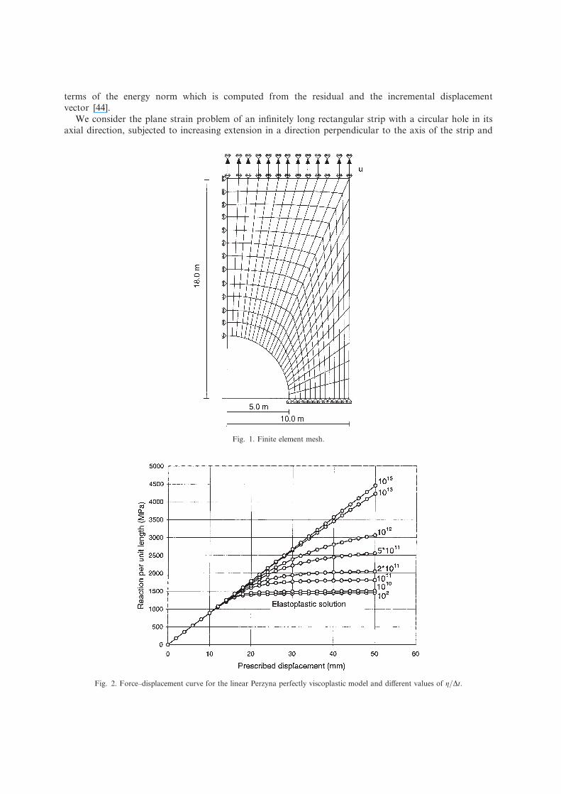
We consider the plane strain problem of an in®nitely long rectangular strip with a circular hole in its

axial direction, subjected to increasing extension in a direction perpendicular to the axis of the strip and

Fig. 1. Finite element mesh.

Fig. 2. Force±displacement curve for the linear Perzyna perfectly viscoplastic model and di�erent values of g=Dt.

5138 G. Alfano et al. / Comput. Methods Appl. Mech. Engrg. 190 !2001) 5123±5147

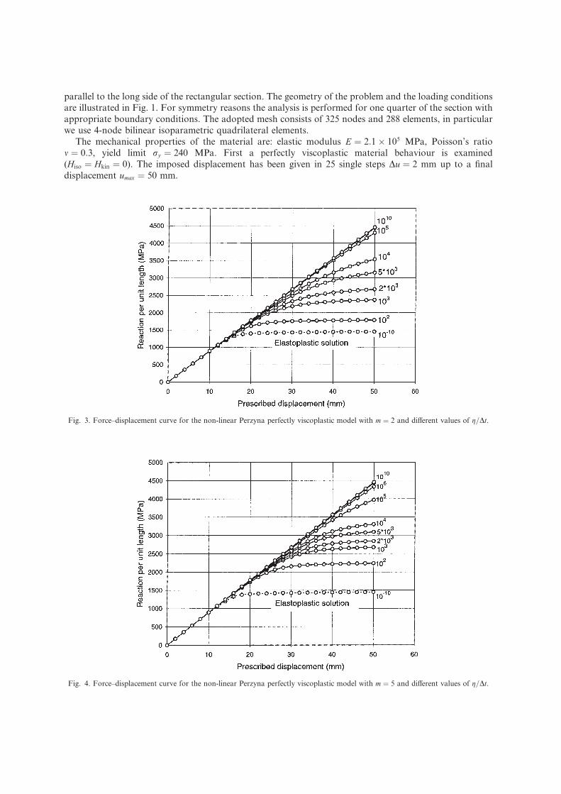
parallel to the long side of the rectangular section. The geometry of the problem and the loading conditions

are illustrated in Fig. 1. For symmetry reasons the analysis is performed for one quarter of the section with

appropriate boundary conditions. The adopted mesh consists of 325 nodes and 288 elements, in particular

we use 4-node bilinear isoparametric quadrilateral elements.

The mechanical properties of the material are: elastic modulus E � 2:1� 105 MPa, Poisson's ratio

m � 0:3, yield limit ry � 240 MPa. First a perfectly viscoplastic material behaviour is examined

!Hiso � Hkin � 0). The imposed displacement has been given in 25 single steps Du � 2 mm up to a ®nal

displacement umax � 50 mm.

Fig. 3. Force±displacement curve for the non-linear Perzyna perfectly viscoplastic model with m � 2 and di�erent values of g=Dt.

Fig. 4. Force±displacement curve for the non-linear Perzyna perfectly viscoplastic model with m � 5 and di�erent values of g=Dt.

G. Alfano et al. / Comput. Methods Appl. Mech. Engrg. 190 !2001) 5123±5147 5139

Di�erent velocities Du=Dt of the imposed displacement are obtained by changing the time increment Dt

relative to the single step.

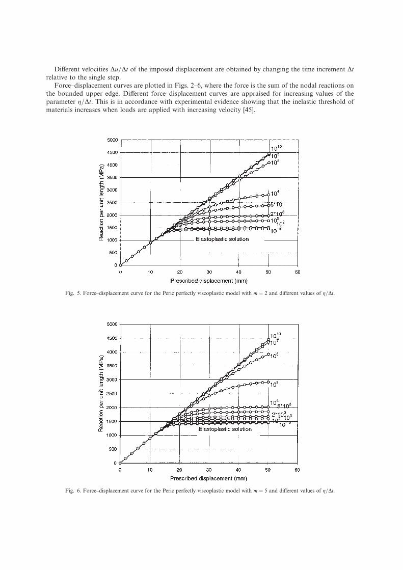
Force±displacement curves are plotted in Figs. 2±6, where the force is the sum of the nodal reactions on

the bounded upper edge. Di�erent force±displacement curves are appraised for increasing values of the

parameter g=Dt. This is in accordance with experimental evidence showing that the inelastic threshold of

materials increases when loads are applied with increasing velocity [45].

Fig. 5. Force±displacement curve for the Peric perfectly viscoplastic model with m � 2 and di�erent values of g=Dt.

Fig. 6. Force±displacement curve for the Peric perfectly viscoplastic model with m � 5 and di�erent values of g=Dt.

5140 G. Alfano et al. / Comput. Methods Appl. Mech. Engrg. 190 !2001) 5123±5147

In Fig. 2 the force±displacement curves given by the linear Perzyna model are plotted. In Figs. 3 and 4

the curves obtained by using the non-linear Perzyna model, for m � 2 and m � 5, respectively, show the

di�erent rate sensitivity.

For the same parameters g=Dt and m, slightly different curves are obtained for the Peric model !Figs. 5

and 6).

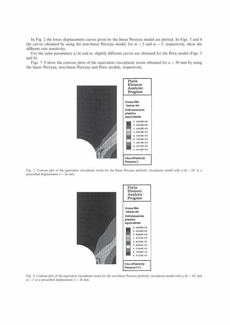
Figs. 7±9 show the contour plots of the equivalent viscoplastic strain obtained for u � 50 mm by using

the linear Perzyna, non-linear Perzyna and Peric models, respectively.

Fig. 7. Contour plot of the equivalent viscoplastic strain for the linear Perzyna perfectly viscoplastic model with g=Dt � 102 at a

prescribed displacement d � 26 mm.

Fig. 8. Contour plot of the equivalent viscoplastic strain for the non-linear Perzyna perfectly viscoplastic model with g=Dt � 103 and

m � 2 at a prescribed displacement d � 26 mm.

G. Alfano et al. / Comput. Methods Appl. Mech. Engrg. 190 !2001) 5123±5147 5141

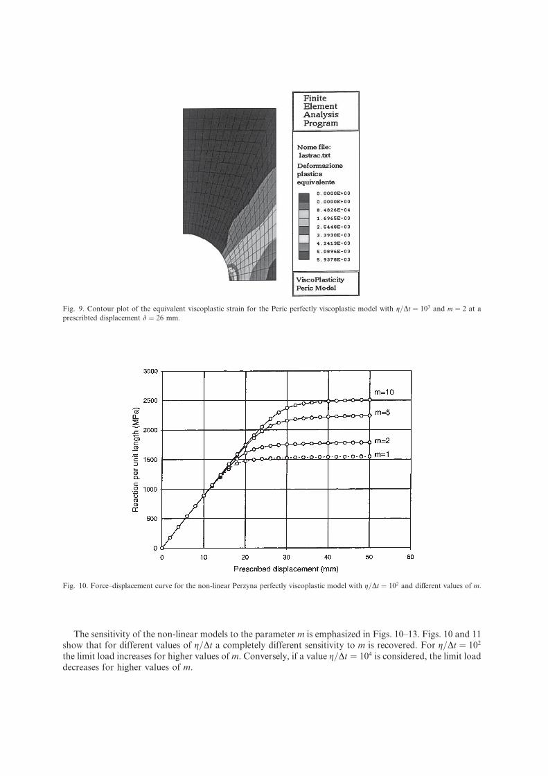
The sensitivity of the non-linear models to the parameter m is emphasized in Figs. 10±13. Figs. 10 and 11

show that for different values of g=Dt a completely different sensitivity to m is recovered. For g=Dt � 102

the limit load increases for higher values of m. Conversely, if a value g=Dt � 104 is considered, the limit load

decreases for higher values of m.

Fig. 9. Contour plot of the equivalent viscoplastic strain for the Peric perfectly viscoplastic model with g=Dt � 103 and m � 2 at a

prescribted displacement d � 26 mm.

Fig. 10. Force±displacement curve for the non-linear Perzyna perfectly viscoplastic model with g=Dt � 102 and di�erent values of m.

5142 G. Alfano et al. / Comput. Methods Appl. Mech. Engrg. 190 !2001) 5123±5147

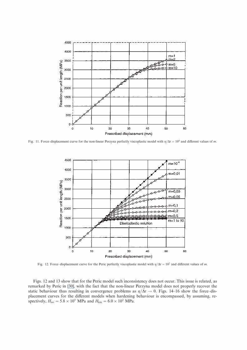
Figs. 12 and 13 show that for the Peric model such inconsistency does not occur. This issue is related, as

remarked by Peric in [30], with the fact that the non-linear Perzyna model does not properly recover the

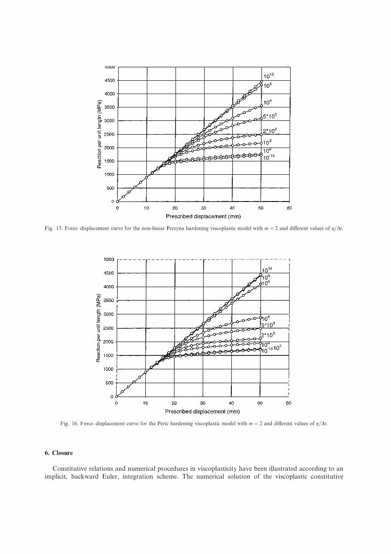
static behaviour thus resulting in convergence problems as g=Dt ! 0. Figs. 14±16 show the force±dis-

placement curves for the di�erent models when hardening behaviour is encompassed, by assuming, re-

spectively, Hiso � 5:8� 103 MPa and Hkin � 6:0� 102 MPa.

Fig. 12. Force±displacement curve for the Peric perfectly viscoplastic model with g=Dt � 102 and di�erent values of m.

Fig. 11. Force±displacement curve for the non-linear Perzyna perfectly viscoplastic model with g=Dt � 104 and di�erent values of m.

G. Alfano et al. / Comput. Methods Appl. Mech. Engrg. 190 !2001) 5123±5147 5143

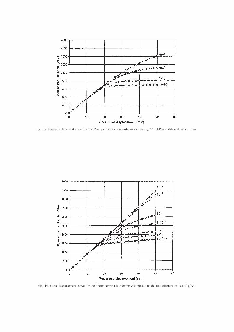
Fig. 13. Force±displacement curve for the Peric perfectly viscoplastic model with g=Dt � 104 and di�erent values of m.

Fig. 14. Force±displacement curve for the linear Perzyna hardening viscoplastic model and di�erent values of g=Dt.

5144 G. Alfano et al. / Comput. Methods Appl. Mech. Engrg. 190 !2001) 5123±5147

6. Closure

Constitutive relations and numerical procedures in viscoplasticity have been illustrated according to an

implicit, backward Euler, integration scheme. The numerical solution of the viscoplastic constitutive

Fig. 16. Force±displacement curve for the Peric hardening viscoplastic model with m � 2 and di�erent values of g=Dt.

Fig. 15. Force±displacement curve for the non-linear Perzyna hardening viscoplastic model with m � 2 and di�erent values of g=Dt.

G. Alfano et al. / Comput. Methods Appl. Mech. Engrg. 190 !2001) 5123±5147 5145

problem has been detailed by following the same lines of reasoning used for the rate-independent models

[41,42,49].

A consistent tangent operator holding for general yield criteria has been derived for elasto/viscoplastic

material models by suitably extending a general procedure exploited for elastoplasticity [2]. The expression

of the tangent operator thus obtained can be used for any viscoplastic model simply by specializing the

expressions of the yield function and of the related ¯ow function.

The expression of the consistent tangent operator which has been derived correctly reduces to the in-

viscid limit for null viscosity parameter so that the case of J2 viscoplasticity [44,49] is recovered.

Numerical examples carried out for a typical benchmark problem have been ®nally reported to assess the

accuracy and robustness of the proposed approach.

Acknowledgements

The authors wish to gratefully acknowledge the Italian Ministry of the University and of the Scienti®c

and Technological Research !MURST) for ®nancial support.

References

[1] G. Alfano, F. De Angelis, L. Rosati, On the derivation of elastoplastic tangent operators from the model of generalized standard

material, in: B.D. Reddy, G.P. Mitchell, R.B. Tait !Eds.), Proceedings of the Second South African Conference on Applied

Mechanics, University of Cape Town, Rondebosch, 1998, pp. 13±24.

[2] G. Alfano, L. Rosati, A general approach to the evaluation of consistent tangent operators for rate-independent elastoplasticity,

Comput. Methods Appl. Mech. Engrg. 167 !1998) 75±89.

[3] F. Auricchio, R.L. Taylor, J. Lubliner, Application of a return map algorithm to plasticity models, in: D.R.J. Owen et al. !Eds.),

Proceedings of the Third International Conference on Computational Plasticity, Pineridge Press, Barcelona, 1992, pp. 2229±2248.

[4] J.L. Chaboche, G. Cailletaud, Integration methods for complex plastic constitutive equations, Comput. Methods Appl. Mech.

Engrg. 133 !1996) 125±155.

[5] M.A. Cris®eld, Non-linear Finite Elements of Solids and Structures, vols. 1±2, Wiley, Chichester, 1991.

[6] F. De Angelis, Constitutive models and computational algorithms in elasto-viscoplasticity, Ph.D. Thesis, University of Naples,

Naples, 1998.

[7] G. Duvaut, J.L. Lions, Les Inequations en Mecanique et en Physique, Dunot, Paris, 1972.

[8] P. Germain, Cours de M�ecanique des Milieux Continus, Masson et Cie, Paris, 1973.

[9] P. Germain, Q.S. Nguyen, P. Suquet, Continuum thermodynamics, J. Appl. Mech. 50 !1983) 1010±1020.

[10] G.H. Golub, C.F. Van Loan, Matrix Computations, John Hopkins University Press, Baltimore, MD, 1989.

[11] B. Halphen, Q.S. Nguyen, Sur les mat�eriaux standards g�en�eralis�es, J. Mech. 14 !1975) 39±63.

[12] R. Hill, The Mathematical Theory of Plasticity, Clarendon Press, Oxford, 1950.

[13] R. Hill, The essential structure of constitutive laws for metal composites and polycrystals, J. Mech. Phys. Solids 15 !1967) 79±95.

[14] J.B. Hiriart-Urruty, C. Lemar�echal, Convex Analysis and Minimization Algorithms, Springer, Berlin, 1993.

[15] T.J.R. Hughes, R.L. Taylor, Unconditionally stable algorithms for quasi-static elasto/viscoplastic ®nite element analysis, Comput.

Struct. 8 !1978) 169±173.

[16] J.W. Ju, Consistent tangent moduli for a class of viscoplasticity, J. Engrg. Mech. 116 !8) !1990).

[17] W.T. Koiter, Stress±strain relations, uniqueness and variational theorems for elastic±plastic materials with a singular yield surface,

Quart. Appl. Math. 11 !1953) 350±354.

[18] W.T. Koiter, General theorems for elastic±plastic solids, Progress in Solids Mechanics 1 !1960) 165±221.

[19] R.D. Krieg, D.B. Krieg, Accuracies of numerical solutions methods for elastic-perfectly plastic model, J. Pressure Vessel Technol.

99 !1977) 510±515.

[20] R.D. Krieg, S.W. Key, Implementation of a time dependent plasticity theory into structural computer programs, in: Constitutive

Equations in Viscoplasticity: Computational and Engineering Aspects, AMD-20, ASME, New York, 1976.

[21] J. Lemaitre, J.L. Chaboche, Mechanics of Solids Materials, Cambridge University Press, Cambridge, 1990.

[22] J. Lubliner, Plasticity Theory, Macmillan, New York, 1990.

[23] D.G. Luenberger, Introduction to Linear and Non-Linear Programming, Addison-Wesley, Reading, MA, 1973.

[24] J. Mandel, Thermodynamics and plasticity, in: J.J. Delgado Domingos, M.N.R. Nina, J.H. Whitelaw !Eds.), Foundations of

Continuum Thermodynamics, Macmillan, New York, 1974, pp. 283±304.

[25] J.J. Moreau, Sur les lois de frottement, de viscosit�e et plasticit�e, C.R. Acad. Sci. 271 !1970) 608±611.

[26] P.M. Naghdi, S.A. Murch, On the mechanical behaviour of viscoelastic/plastic solids, J. Appl. Mech. 30 !1963) 321±328.

[27] J.C. Nagtegaal, On the implementation of inelastic constitutive equations with special reference to large deformation problems,

Comput. Methods Appl. Mech. Engrg. 33 !1982) 469±484.

5146 G. Alfano et al. / Comput. Methods Appl. Mech. Engrg. 190 !2001) 5123±5147

[28] Q.S. Nguyen, On the elastic plastic initial-boundary value problem and its numerical integration, Int. J. Numer. Methods Engrg.

11 !1977) 817±832.

[29] M. Ortiz, E.P. Popov, Accuracy and stability of integration algorithms for elastoplastic constitutive relations, Int. J. Numer.

Methods Engrg. 21 !1985) 1561±1576.

[30] D. Peric, On a class of constitutive equations in viscoplasticity: formulation and computational issues, Int. J. Numer. Methods

Engrg. 36 !1993) 1365±1393.

[31] D. Peirce, C.F. Shih, A. Needleman, A tangent modulus method for rate dependent solids, Comput. Struct. 18 !1984) 875±887.

[32] P. Perzyna, The constitutive equations for rate sensitive materials, Quart. Appl. Math. 20 !1963) 321±332.

[33] P. Perzyna, Fundamental problems in viscoplasticity, Adv. Appl. Mech. 9 !1966) 243±377.

[34] P. Perzyna, Thermodynamic theory of viscoplasticity, Adv. Appl. Mech. 11 !1971) 313±354.

[35] J.R. Rice, On the structure of stress±strain relations for time-dependent plastic deformation in metals, J. Appl. Mech. 137 !1970)

728±737.

[36] J.R. Rice, Inelastic constitutive relations for solids: an internal variable theory and its application to metal plasticity, J. Mech.

Phys. Solids 19 !1971) 433±455.

[37] R.T. Rockafellar, Convex Analysis, Princeton University Press, Princeton, 1970.

[38] G. Romano, L. Rosati, F. Marotti de Sciarra, An internal variable theory of inelastic behaviour derived from the uniaxial rigid-

perfectly plastic law, Int. J. Engrg. Sci. 31 !1993) 1105±1120.

[39] J.C. Simo, Nonlinear stability of the time-discrete variational problem of evolution in nonlinear heat conduction, plasticity and

viscoplasticity, Comput. Methods Appl. Mech. Engrg. 88 !1991) 111±131.

[40] J.C. Simo, Algorithms for static and dynamic multiplicative plasticity that preserve the classical return mapping schemes of the

in®nitesimal theory, Comput. Methods Appl. Mech. Engrg. 99 !1992) 61±112.

[41] J.C. Simo, S. Govindjee, Non-linear B-stability and symmetry preserving return mapping algorithms for plasticity and

viscoplasticity, Int. J. Numer. Methods Engrg. 31 !1991) 151±176.

[42] J.C. Simo, T. Honein, Variational formulations, discrete conservation laws, and path-domain independent integrals for elasto-

viscoplasticity, J. Appl. Mech., Trans. ASME 57 !1990) 488±497.

[43] J.C. Simo, J.J. Kennedy, S. Govindjee, Non-smooth multisurface plasticity and viscoplasticity. Loading/unloading conditions and

numerical algorithms, Int. J. Numer. Methods Engrg. 26 !1988) 2161±2185.

[44] J.C. Simo, R.L. Taylor, Consistent tangent operators for rate-independent elastoplasticity, Comput. Methods Appl. Mech. Engrg.

48 !1985) 101±118.

[45] J.J. Skrzypek, R.B. Hetnarski, Plasticity and Creep, CRC Press, Boca Raton, FL, 1993.

[46] P.M. Suquet, Sur les equations de la plasticit�e: existence et r�egularit�e des solutions, J. M�ecanique 20 !1981) 3±39.

[47] L. Szabo, Evaluation of elasto-viscoplastic tangent matrices without numerical inversion, Comput. Struct. 21 !6) !1985) 1235±

1236.

[48] L. Szabo, Tangent modulus tensors for elastic-viscoplastic solids, Comput. Struct. 34 !3) !1990) 401±419.

[49] R.L. Taylor, Computational Mechanics Notes, Version 2.0, Department of Civil and Environmental Engineering, Berkeley, 1998.

[50] R. Temam, Mathematical Problems in Plasticity, Gautier-Villars, Paris, 1985.

[51] E. Voce, Metalurgica 51 !1955) 219.

[52] M.L. Wilkins, Calculation of elastic±plastic ¯ow, in: B. Alder et al. !Eds.), Methods of Computational Physics, vol. 3, Academic

Press, New York, 1964.

[53] K. Yosida, Functional Analysis, Springer, Berlin, 1980.

[54] O.C. Zienkiewicz, I.C. Cormeau, Visco-plasticity, plasticity and creep, a uni®ed numerical solution approach, Int. J. Numer.

Methods Engrg. 8 !1974) 821±845.

[55] O.C. Zienkiewicz, R.L. Taylor, The Finite Element Method, fourth ed., vols. 1±2, McGraw-Hill, London, 1991.

G. Alfano et al. / Comput. Methods Appl. Mech. Engrg. 190 !2001) 5123±5147 5147