Jump or Kink? Regression Probability Jump and Kink

Design for Treatment Effect Evaluation

Yingying Dong∗

Department of Economics

University of California Irvine

This version: July 2017

Abstract

This paper evaluates the impacts of participation in two social programs: elite school

attendance in the United Kingdom and compulsory military service in Russia. A common

feature of the two programs is that each entails a binary treatment, and the treatment as-

signment rule exhibits a dramatic kink with little or no jump. As a result, the standard

RD design does not work well empirically. This paper extends the standard RD design

with a binary treatment to allow for causal identification under more general conditions.

I show that without a jump, one can still identify a causal effect utilizing a slope change

(a kink) in the treatment probability. This kink based identification requires only minimal

further smoothness relative to the standard RD design. The required smoothness is readily

satisfied given a weak and testable behavioral assumption. I then propose a new Regres-

sion Probability Jump and Kink (RPJK) design that is valid regardless of whether there is

a jump, or a kink, or both in the treatment probability. In sharp contrast to the results of

the standard RD design, the proposed identification approaches yield plausible estimates

of causal impacts in the two social programs under consideration.

JEL Codes: C21, C25, I90, J100

Keywords: Regression discontinuity (RD) design, Marginal treatment effect (MTE), Local

average treatment effect (LATE), Regression probability kink (RPK) design, Regression

probability jump and kink (RPJK) design

∗Correspondence: Department of Economics, 3151 Social Science Plaza, University of California Irvine, CA 92697-

5100, USA. Email: yyd@uci.edu. http://yingyingdong.com/.

The author would like to thank Arthur Lewbel, Joshua Angrist, James Heckman, Han Hong, Damon Clark, Marianne

Bitler, Ping Yu, and four anonymous referees for very helpful comments, and thank Damon Clark and Emilia Del Bono for

making their data available. Thanks also go to seminar participants at UCI, CSULB, CUHK, BC, MIT and UCR, as well

as conference participants at the SOLE, CEA, WEAI, and AMES annual conferences. Any errors are my own.

1

1 Introduction

Many public policies or social programs set explicit eligibility thresholds for treatment. It may then

be possible to evaluate program effects locally near the policy threshold. The standard regression

discontinuity (RD) design relies on a discrete change (i.e., a jump) in the treatment probability to

identify a causal effect of treatment. Identification fails when there is no discontinuity, or is weak when

the discontinuity is small. See discussions in Imbens and Lemieux (2008), chapter 6 of Angrist and

Pischke (2008), Imbens and Wooldridge (2009), and Lee and Lemieux (2010).

This paper evaluates the impacts of participation in two social programs: elite school attendance in

the United Kingdom and compulsory military service in Russia. Despite the very different institutions,

a common feature of the two programs is that each entails a binary treatment, and the treatment assign-

ment rule exhibits a dramatic kink with little or no jump. As a result, the standard RD design does not

work well empirically.

To accommodate empirical scenarios similar to the above, this paper extends the standard RD

design with a binary treatment to allow for causal identification under more general conditions. In

particular, I discuss identification using a kink instead of, or in addition to, a jump in the treatment

probability. I show that identification using a kink in the treatment probability is valid under minimal

further smoothness conditions than those required by the standard RD design. While the standard RD

design identifies a local average treatment effect (LATE), a kink in the treatment probability generally

identifies a marginal treatment effect (MTE), which can be interpreted as a limiting form of LATE (see

Heckman and Vytlacil, 2005, 2007, and Carneiro, Heckman, and Vytlacil, 2010).

Note that this paper considers a binary treatment. In contrast, the recent regression kink (RK)

design (Card, Lee, Pei, and Weber, 2015) considers a continuous treatment.1 I therefore refer to the

new kink design proposed here as the regression probability kink (RPK) design.

Just as a jump in the standard RD design is generated by the policy rule, kinks in treatment prob-

abilities should likewise be dictated by policy rules. For example, in Clark and Del Bono (2016), the

elite school assignment rule is based on an assignment score. Below a certain low threshold score, one

is ineligible for the treatment, i.e., of attending an elite school, so the probability of treatment is nearly

zero. Once above a certain high threshold, one is eligible (with some exceptions), so the probability of

1Their sharp RK design differs from the RPK design and leads to a different estimand. Their fuzzy RK design leads to an

estimand that is comparable to the RPK estimand; However, the design setup, the interpretation of the identified parameter,

and the identifying assumptions are entirely different.

2

treatment is almost one. Students in between the two thresholds are ordered based on merit, and so the

further one’s score is above the low threshold, the greater is the probability of treatment. As a result of

this assignment rule, at each of these two thresholds there is a large kink, and little or no jump, in the

probability of attending an elite school.

As another example, demilitarization in Russia leads to a kinked profile in the induction rate across

birth cohorts after the cold war (Card and Yakovlev 2014). Such a steady rather than sudden change in

the share of men drafted into the military can be justified on the grounds of reducing adjustment costs.

Analogous to the standard RD design, identification based on kinks also requires that individuals cannot

precisely manipulate the running variable (e.g., the assignment score or birth date), so random chance

determines whether one falls just above or just below the kink point.

Let T be a binary treatment indicator, such as attending an elite school, or serving in the army. Let R

be the so-called running or forcing variable, such as a test score or birth date. Treatment is determined

at least in part by whether the the running variable crosses a known threshold value r0. Let Z = I {R ≥

r0}, where I {·} is an indicator function equal to 1 if the expression in the bracket is true and 0 otherwise.

Assume T = 1 {P (R)−U ≥ 0}, where U is normalized to follow a uniform distribution over the unit

interval. Without loss of generality, one can rewrite T = 1 {P1 (R) Z + P0 (R) (1− Z)−U ≥ 0} =

1 {P1 (R)−U ≥ 0} Z+1 {P0 (R)−U ≥ 0} (1− Z), where the function 1 {Pz (R)−U ≥ 0}, z = 0, 1

describes the assignment of treatment below or above the threshold. For example, the elite school

assignment rule near the low eligibility threshold r0 features P0 (R) = 0 and locally linear probability

P1 (R) = a + b(R − r0) for some coefficients a and b.

More generally, a kink in a choice probability can arise from a kinked cost or benefit schedule for

the choice. Assume that P (R) is a (normalized) cost schedule, while U represents the (normalized)

willingness-to-pay for the treatment. A kinked cost schedule implies d P0 (r) /dr |r06= d P1 (r) /dr |r0

,

which is a kink in the treatment probability. For example, Simonsen, Skipper and Skipper (2016)

show that due to a kinked reimbursement schedule for prescription drugs, the probability of purchasing

prescription drugs is a kinked function of total medical spending. In addition, Nielsen, Sørensen, and

Taber (2010) note that college financial aid is a kinked function of parental income, and consequently,

there is a kinked relationship between the probability of college enrollment and parental income.2

Frequently, the treatment probability may show both a jump and a kink at some policy threshold.

2In fact, RK designs are often applied in situations where the outcome is binary, even though they generally require

continuous treatment. An RK design with a binary outcome (as exemplified by the above two studies) implies a kink in the

probability of that outcome.

3

For example, serving in the Russian army during the demilitarization after the Cold War features this.

I therefore discuss a general research design, the regression probability jump and kink (RPJK) design.

The RPJK design is valid regardless whether there is a jump, a kink, or both in the treatment probabil-

ity. It incorporates the standard RD design and the RPK design as special cases. This general RPJK

design is especially useful when an empirically observed jump is small or statistically insignificant. I

propose a simple local two stage least squares (2SLS) estimator for the RPJK design, and show that

the corresponding estimand is asymptotically equivalent to the standard RD estimand when there is a

real jump in the treatment probability, and otherwise reduces to the RPK estimand.

These new identification results make it possible to evaluate causal effects of the two programs

under consideration. In both cases, any jump that might be present is too small for the standard RD

estimators to work.3 In contrast, the proposed RPK and RPJK designs yield plausible estimates. For

example, in the evaluation of elite school attendance, I confirm previous estimates resulted from a

parametric constant effect model, and in the evaluation of compulsory military service, I estimate sig-

nificant negative impacts that are consistent with economic theory when education is interrupted and

entry into the labor force is delayed. These negative effects, induced by the particular institutional set-

ting in Russia, are in sharp contrast to the prevailing evidence from the US and other OECD countries.

Other related topics, such as identifying complier (or marginal complier) characteristics and check-

ing for monotonicity, in addition to the usual tests for smoothness conditions, are briefly discussed.

The rest of the paper is organized as follows. Section 2 discusses the RPK design. Section 3

discusses the more general RPJK design that allows for either a jump, a kink, or both in the treatment

probability. Section 4 relates the identification results to instrumental variables estimation and provides

a local 2SLS estimator that is valid regardless of whether there is a jump, a kink, or both in the treatment

probability. Section 5 discusses identification of other parameters of interest and provides checks

for the underlying model assumptions. Sections 6 and 7 evaluate the UK elite school and Russian

demilitarization programs by the proposed approaches. Section 8 concludes.

3It is possible to apply the results of Feir, Lemieux and Marmer (2016) to deal with weak identification in standard RD

designs; however, this practice is by ignoring another possible sources of identification, slope changes.

4

2 Regression Probability Kink (RPK) Design

This section first presents the RPK design by the MTE framework, and then discusses equivalent results

using the Angrist, Imbens, and Rubin (AIR) framework (Imbens and Angrist 1994, Angrist, Imbens,

and Rubin 1996).

2.1 RPK Identification 4

Let Y denote the outcome of interest. Assume Y = g(R, T,W ), where the unobservable W is allowed

to be multidimensional. The binary treatment indicator T is endogenous, since it can be correlated with

the running variable R and the unobservables W .5 For notational convenience, define Yt ≡ g(R, t,W )

for t = 0, 1. Y1 and Y0 are an individual’s potential outcomes from being treated or not, respectively

(Neyman, 1923, Rubin, 1974, Gronau, 1974, Heckman 1974, Quandt, 1972). The observed outcome

of interest can then be written as Y = Y1T + Y0 (1− T ).

Let F·|·(·|·) denote a conditional cumulative density function, and f·(·) denote an unconditional

probability density function. The following assumption holds for r ∈ (r0 − ε, r0 + ε) for some small

ε > 0.

Assumption:

A1 (Selection Model): Assume T = 1 {P (R)−U ≥ 0}, where U ∼ Uni f (0, 1).

A2 (Smoothness): P (r) is continuously differentiable everywhere in r ∈ (r0 − ε, r0 + ε) except at

r = r0. E [Yt |U = u, R = r ], t = 0, 1, is continuously differentiable. E [|Yt ||U = u, R = r ] < ∞.

The density of the running variable fR (r) is continuous and strictly positive at r = r0.

A1 assumes that U follows a uniform distribution, which is simply a free normalization (Vyt-

lacil, 2002). More generally if T = 1 {h (R)− V ≥ 0}, where the conditional distribution of V

given R, FV |R (V |R), is strictly increasing, then one can let U ≡ FV |R (V |R) ∼ Uni f (0, 1) and

P (R) ≡ FV |R (h (R) |R). Vytlacil (2002) shows that Assumption A1 is equivalent to the monotonic-

ity assumption of the LATE model (Imben and Angrist, 1994, Angrist, Imbens, and Rubin, 1996). In

Section 5, I briefly discuss how one can check for monotonicity in empirical applications.

A2 is a smoothness parallel of the independence assumption required to identify LATE or MTE. For

example, Vytlacil (2002, Assumption S-1, (ii)) assumes a binary instrumental variable Z ⊥ (U, Y0, Y1)

4This section benefited from constructive suggestions from one of the anonymous referees.5All of the functions defined here could also depend on additional covariates X , which are omitted for clarity.

5

to identify LATE. Heckman and Vytlacil, (2007, section 6) assume a continuous instrumental variable

Z ⊥ (U, Yt), t = 0, 1, to identify MTE.6

Before providing formal theorems, I first define LATE and MTE in the present context, and obtain

some required equalities. Since T = 1 {P (R)−U ≥ 0}, P (r) = E [T |R = r ]. Similarly define

G (r) ≡ E [Y |R = r ]. The following discussion utilizes one-sided limits and one-sided derivatives at

r = r0. For any function H(r), let H+ ≡ limr↓r0H(r) and H− ≡ limr↑r0

H(r) be the right and left

limits, respectively, when they exist. Further let H ′+ ≡ limr↓r0∂H(r)/∂r and H ′− ≡ limr↑r0

∂H(r)/∂r

be the right and left derivatives, respectively, when they exist. Then define

τ L AT E (P+, P−, r0) ≡ E[Y1 − Y0|P− < U ≤ P+, r = r0

].

Further define an MTE parameter as follows,

τMT E (u, r) ≡ E [Y1 − Y0|U = u, R = r ] .

For simplicity, when the MTE is evaluated at r0, let τMT E (u) ≡ E [Y1 − Y0|U = u, r = r0].

When there is a jump in the treatment probability at r0, P+ 6= P−, and then τ L AT E (P+, P−, r0) =

1P+−P−

∫ P+P−

E [Y1 − Y0|U = u, R = r0] du = 1P+−P−

∫ P+P−τMT E (u) du. When there is no jump, P+ =

P− = P (r0), and hence τ L AT E (P+, P−, r0) = τMT E (P (r0)) by definition. Under Assumptions A1

and A2, when P+ 6= P−, τ L AT E (P+, P−, r0) =G+−G−P+−P−

, as shown in Hahn, Todd, and van der Klaauw

(2001).

Rewrite Y = αT + Y0, where α ≡ Y1 − Y0. Then

G (r) ≡ E [Y |R = r ]

= E [α1 {U ≤ P (r)} |R = r ]+ E [Y0|R = r ]

=

∫ P(r)

0

E [α|U = u, R = r ] du + E [Y0|R = r ] . (1)

By A2, E [α|U = u, R = r ] and E [Y0|R = r ] are continuously differentiable in r , since E [Y0|R = r ] =∫ 1

0E [Y0|U = u, R = r ] du, and under standard regularity conditions (when dominated convergence

6More recently, Chiang and Sasaki (2017) extend this paper’s RPK setup to further identify quantile treatment effects

(QTEs). They impose smoothness on the conditional cumulative distribution function FYt |U,R (y|u, r) instead of the condi-

tional mean function E [Yt |U = u, R = r ], t = 0, 1.

6

theorem holds), one can differentiate under the integral sign. Further by A2, P (r) is continuously

differentiable in r ∈ (r0 − ε, r0 + ε) \ {r0}, then∫ P(r)

0E [α|R = r,U = u] du is continuously differ-

entiable in r ∈ (r0 − ε, r0 + ε) \ {r0} by applying Leibniz’ rule.

Taking right and left limits at r = r0 on both sides of equation (1) yields

G+ − G− = limr↓r0

∫ P(r)0

E [α|R = r,U = u] du − limr↑r0

∫ P(r)0

E [α|R = r,U = u] du

= E[α1 {U ≤ P+} |R = r0

]− E

[α1 {U ≤ P−} |R = r0

]= E

[α1 {P− < U ≤ P+} |R = r0,

]= E

[Y1 − Y0|P− < U ≤ P+, R = r0

](P+ − P−) .

Therefore, we obtain the familiar fuzzy RD estimand

τ L AT E (P+, P−, r0) ≡ E[Y1 − Y0|P− < U ≤ P+, R = r0

]=

G+ − G−

P+ − P−. (2)

Now consider the case where there is no jump, but a kink in the treatment probability, i.e., P+ = P−

and P ′+ 6= P ′−.

Theorem 1 Suppose that Assumptions A1 and A2 hold. If P+ = P−, and P ′+ 6= P ′−, then

τMT E (P (r0)) =G ′+ − G ′−

P ′+ − P ′−.

First notice that for r ∈ (r0 − ε, r0 + ε) \ {r0},

∂

∂rG (r) = P ′ (r) E [α|U = P (r) , R = r ]+

∫ P(r)

0

∂

∂rE [α|U = u, R = r ] du +

∂

∂rE [Y0|R = r ] .

(3)

Then because E [α|U = u, R = r ] and E [Y0|R = r ] are continuously differentiable in r , taking

right and left limits at r = r0 on both sides of equation (3) yields

G ′+ − G ′− = P ′+E[α|U = P+, R = r0

]− P ′−E

[α|U = P−, R = r0

]+

∫ P+

0

∂

∂rE [α|U = u, R = r ] |r0

du −

∫ P−

0

∂

∂rE [α|U = u, R = r ] |r0

du

= P ′+τMT E (P+)− P ′−τMT E (P−)+

∫ P+

P−

∂

∂rE [α|U = u, R = r ] |r0

du. (4)

7

When there is no jump, P+ = P− = P (r0), then equation (4) reduces to G ′+−G ′− =(P ′+ − P ′−

)τMT E (P (r0)).

Therefore,

τMT E (P (r0)) ≡ E [Y1 − Y0|U = P (r0) , R = r0] =G ′+ − G ′−

P ′+ − P ′−. (5)

That is, when there is no jump, but a kink, the ratio of kinks above identifies an average treatment

effect for marginal compliers at r = r0. Assuming T = 1 {P (R) ≥ U }, marginal compliers are

individuals with U = P (r0), i.e., they are just indifferent to being treated or not at the kink point.

2.2 AIR Framework Representation

This section re-casts the identification results in the previous section in the AIR framework. To that

end, assume T = h (R, V ) for some unobservable V . Given Z = 1 {R ≥ r0}, one can rewrite T =

h1 (R, V ) Z + h0 (R, V ) (1− Z).

For an individual with R = r , define Tz (r) ≡ hz (r, V ), z = 0, 1, as her potential treatment status

if she is below or above the cutoff. The following extends the definitions of individual types in Imbens

and Angrist (1994) and Angrist, Imbens, and Rubin (1996) to the RD setup. In a common probability

space (�, F , P), always taker A (r) is the event that T1 (r) = T0 (r) = 1; never taker N (r) is the event

that T1 (r) = T0 (r) = 0; complier C (r) is the event that T1 (r)− T0 (r) = 1; defier D (r) is the event

that T1 (r) − T0 (r) = −1. For simplicity, whenever there is no confusion, I will use A, N , C, and D

to denote individual types, and similarly use Tz to denote Tz (r), z = 0, 1. Let S ≡ (Y1, Y0, T1, T0).

The following assumption holds for r ∈ (r0 − ε, r0 + ε).

Assumption:

B1 (Monotonicity): Pr (D (r)) = 0 for all r ∈ (r0 − ε, r + ε).

B2 (Smoothness): FS|R (s|r) is continuously differentiable for all s ∈ supp (S). fR(r) is continu-

ous and strictly positive at r = r0.

B1 is the standard assumption ruling out defiers, so changes in treatment status can only be in one

direction. This assumption is equivalent to A1 in the previous section (Vytlacil, 2002). By A1, T =

1 {P (R)−U ≥ 0}. Without loss of generality, rewrite it as T = 1 {P0 (R) (1− Z)+ P1 (R) Z ≥ U }.

Then C (r) are individuals with P0 (r)< U ≤ P1 (r) and C (r0) are individuals with P−< U ≤ P+.

When P+ − P− 6= 0, τ L AT E (P+, P−, r0) defined previously is then E [Y1 − Y0|C, R = r0] in this

section’s notation.

8

B2 assumes that the joint distribution of (Y0, Y1, T0, T1) given the running variable R is smooth in

the neighborhood of r0. B2 is a smoothness parallel of the LATE type independence assumption in the

causal model framework (see, e.g., Imbens and Angrist, 1994), which requires (Y0, Y1, T0, T1) to be

independent of a binary instrument. Here the binary instrumental variable (IV) is Z = I {R ≥ r0}.

Further B2 implies that E [Yt |R = r,2] for t = 0, 1 and Pr (2|R = r) for 2 ∈ {A, N ,C, D} are

continuously differentiable in the neighborhood of r = r0. These weaker conditions are sufficient to

identify mean treatment effects. In contrast, B2 is sufficient, but stronger than necessary. B2 can be

used to identify distributional effects as discussed in Frandsen, Frölich, and Melly (2012).

B2 allows for essential heterogeneity of treatment effects and self-selection into different types,

since no restrictions are imposed on the joint distribution of (Y0, Y1, T0, T1). For example, individuals

may self-select to be compliers for higher idiosyncratic gains. Following the arguments in Lee (2008)

and McCrary (2008), B2 in practice implies that individuals can not precisely manipulate the running

variable to sort around the RD threshold.

Continuous differentiability in B2 or A2 rules out not only jumps but also kinks. One can therefore

perform falsification tests to test smoothness (no jumps and kinks) of the conditional means of covari-

ates, conditional on the running variable. Alternatively, one may perform the ‘manipulation’ tests as in

McCrary (2008).

Theorem 2 Assume that B1 and B2 hold. P+−P− = Pr (C |R = r0) and P ′+−P ′− =∂∂r

Pr (C |R = r) |r0.

Further if P+ 6= P−, then (G+ − G−) / (P+ − P−) = E [Y1 − Y0|C, R = r0]; otherwise, as P+ −

P−→ 0, τ L AT E (P+, P−, r0)→ τMT E (P (r0)), and when P ′+ 6= P ′−,

τMT E (P (r0)) =G ′+ − G ′−

P ′+ − P ′−. (6)

Theorem 2 states that given a kink, when the jump goes arbitrarily close to zero,(G ′+ − G ′−

)/(P ′+ − P ′−

)identifies a limiting form of RD LATE, τMT E (P (r0)). The probability of compliers or the compliance

rate is a function of r by definition. Under B1 and B2, a jump in the treatment probability exists if the

compliance rate at r = r0 is not zero, while a kink exists if the derivative of the compliance rate at

r = r0 is not zero.7

7Given monotonicity, one can assume that the treatment is generated by T ≡ 1 {P (R) ≥ U }. Then when P+ = P− ,

what is in the conditioning set of τ L AT E (P+, P−, r0) is U = P (r0), namely marginal compliers at r = r0.

9

3 Regression Probability Jump & Kink (RPJK) Design

The discussion so far has given a causal interpretation of the kink estimand when there is no jump in

the treatment probability at the RD threshold. This section now considers what happens when a jump

might be present. I first show that when both a jump and a kink are present, the kink estimand generally

loses its causal interpretation. I then discuss causal identification regardless of whether there is a jump,

or a kink, or both by a RPJK design.

By assumption A1, T = 1 {P (R)−U ≥ 0}. Without loss of generality, rewrite it as T =

1 {P0 (R) (1− Z)+ P1 (R) Z ≥ U }. To facilitate the discussion in this section, assume smoothness

of Pz (r).

Assumption:

A3 (Smoothness): Pz (r), z = 0, 1, is continuously differentiable in r for r ∈ (r0 − ε, r0 + ε).8

By Assumption A3, P+ = P1 (r0), P− = P0 (r0), P ′+ =∂∂r

P1 (r) |r0, and P ′− =

∂∂r

P0 (r) |r0. Then

when P1 (r) 6= P0 (r), define

τ (r) ≡ τ L AT E (P1 (r) , P0 (r) , r) ≡ E [α|P0 (r) ≤ U ≤ P1 (r) , R = r ]

=1

P1 (r)− P0 (r)

∫ P1(r)

P0(r)τMT E (u, r) du, (7)

so τ (r0) = τ L AT E (P+, P−, r0), and further define τ ′ (r0) ≡∂∂rτ (r) |r0

.9 By equation (7),

τ (r) (P1 (r)− P0 (r)) =

∫ P1(r)

P0(r)τMT E (u, r) du. (8)

8Section 2 only assumes smoothness of the actual propensity score P(r). This section further assumes smoothness

of the potential Pz(r) to define τ ′ (r0) after equation (7). As I will show, τ ′ (r0) partly depends on how the size of jump

P1 (r)− P0 (r) changes with the running variable r (given the fixed threshold r0) near r0.

9τ ′ (r0)measures how the treatment effect varies with the running variable near the fixed threshold r0. Dong and Lewbel

(2015) refer to τ ′ (r0) as the treatment effect derivative (TED) and show that TED is nonparametrically identified given a

jump in the treatment probability and the smoothness conditions in this paper. Cerulli, Dong, Lewbel, and Poulsen (2017)

show how TED can be used to test stability and hence external validity of RD estimates.

10

Taking derivatives on both sides of equation (8) at r = r0 yields

τ ′ (r0) (P+ − P−)+ τ (r0)(P ′+ − P ′−

)=

∂

∂r

(∫ P1(r)

P0(r)τMT E (u, r) du

)|r0

= P ′+τMT E (P+)− P ′−τMT E (P−)+

(∫ P+

P−

∂

∂rτMT E (u, r) |r0

du

)= G ′+ − G ′−,

where the last equality follows from equation (4). If both a jump and a kink are present, i.e., P ′+ 6= P ′−

and P+ 6= P−, thenG ′+ − G ′−

P ′+ − P ′−= τ (r0)+

P+ − P−

P ′+ − P ′−τ ′ (r0) . (9)

That is, the RPK estimand no longer equals the causal parameter unless τ ′ (r0) = 0. The potential

bias is given by (P+ − P−) τ′ (r0) /

(P ′+ − P ′−

). Using the AIR framework, the proof of Theorem 2

similarly shows G ′+ − G ′− = τ′ (r0) (P+ − P−)+ τ (r0)

(P ′+ − P ′−

), and hence equation (9) holds.10

The following Theorem provides a way to identify a causal effect regardless of whether there is a

jump, a kink, or both.

Theorem 3 Assume that A1 and A2 hold. Further assume that P+ − P− = 0 and P ′+ − P ′− = 0 do

not both hold (i.e., there is either a jump, or a kink, or both). Given any sequence of nonzero weights

ωn such that limn→∞ ωn = 0,

τ L AT E (P+, P−, r0) = limωn→0

G+ − G− + ωn

(G ′+ − G ′−

)P+ − P− + ωn

(P ′+ − P ′−

) . (10)

Let ηn =G+−G−+ωn(G ′+−G ′−)P+−P−+ωn(P ′+−P ′−)

be a ‘drifting parameter’ that changes with sample size n. Theorem 3

then shows that τ L AT E (P+, P−, r0) equals the limit of this drifting parameter. When there is no jump,

P+ − P− = 0 and G+ − G− = 0, making τ L AT E (P+, P−, r0) = τMT E (P (r0)), and equation (10)

becomes the RPK estimand. When there is a jump, then regardless of whether there is a kink or not,

equation (10) becomes the standard RD estimand.

Here the sequence ωn is required to go to zero as the sample size goes to infinity. The next section

10See equation (18) and the discussion in the proof of Theorem 2. In the AIR model notation, RD

LATE is equivalently defined as τ (r0) ≡ E [Y1 − Y0|C (r0) , R = r0]. Further, TED is equivalently defined as

τ ′ (r0) ≡∂∂r

E [Y1 − Y0|C (r) , R = r ] |r0, because assuming T = 1 {P0 (R) (1− Z)+ P1 (R) Z ≥ U }, those with

P0 (r)< U ≤ P1 (r) are C (r).

11

shows that the weights in a local 2SLS estimator, a special case of the estimator corresponding to

Theorem 3, have this property. Equation (10) (and its special case, the local 2SLS discussed later) has

the advantage that it provides a way to identify a valid causal effect if one is unsure whether a jump is

present or not.

The following Corollary 1a shows the conditions under which the RPK estimand and the standard

RD estimand identify the same parameter, and so in this special case both could be used.

Corollary 1a Assume that A1, A2, and A3 hold, and τ ′ (r0) = 0. If P+ 6= P− and P ′+ 6= P ′−, i.e., both

a jump and a kink exist, then

τ L AT E (P+, P−, r0) =G+ − G−

P+ − P−=

G ′+ − G ′−

P ′+ − P ′−.

τ ′ (r0) = 0 when the treatment effect is locally constant.11 Having τ ′ (r0) = 0 is a strong restriction

that is not required anywhere else in this paper. By equation (9), τ ′ (r0) =G ′+−G ′−P+−P−

−P ′+−P ′−P+−P−

τ (r0), which

is estimable when P+ 6= P− and hence τ ′ (r0) = 0 is a testable restriction.12

When τ ′ (r0) = 0, the jump estimand and the kink estimand are both equal, and hence both can be

used. Similarly, Heckman and Vytlacil (2005) note that when the treatment effect is (locally) constant,

LATE equals its limiting MTE value.

Corollary 1b Assume that A1, A2, and A3 hold, and τ ′ (r0) = 0. If either a jump, or a kink, or both

exist, then

τ L AT E (P+, P−, r0) =G+ − G− + ω

(G ′+ − G ′−

)P+ − P− + ω

(P ′+ − P ′−

) (11)

for any ω 6= − (P+ − P−) /(P ′+ − P ′−

).

Unlike Theorem 3, Corollary 1b employs fixed weights ω, and so exploits both the jump and the

kink when both are present. Lastly, it is worth mentioning that the above results can be readily extended

to identification using higher-order derivative changes at the RD threshold. Further discussion of this

is provided in Appendix III.

11τ ′ (r0) = 0 is a strictly weaker condition than assuming a locally constant treatment effect, because the latter would

imply that all derivatives of τ (r) at r = r0 were zero, not just the first derivative τ ′ (r0).12For example, one can estimate τ ′ (r0) as the coefficient of T (R − r0) in a local linear regression of Y on

T , (R − r0) and T (R − r0). Alternatively, one can directly estimate τ ′ (r0) =(G ′+ − G ′−

)/ (P+ − P−) −

(G+ − G−)(P ′+ − P ′−

)/ (P+ − P−)

2. Details can be found in Dong and Lewbel (2015).

12

4 Instrumental Variable Interpretation and Local 2SLS estima-

tion

This section relates the identification results to instrumental variable (IV) models. Like all RD type

estimators, the 2SLS estimator discussed in this section has a bandwidth that shrinks to zero as the

sample size goes to infinity. It is therefore referred to as a local 2SLS estimator. When there is either

a jump, or a kink, or both, the local 2SLS estimator proposed here automatically provides weights

that satisfy the properties required by Theorem 3. For ease of exposition, I assume a uniform kernel

for the discussion in this section. Using more complicated kernel functions would just complicate the

presentation, but not the conclusions in this section.

Consider the following local linear regression representation of Y for R ∈ (r0 − ε, r0 + ε),

Y = a + b(R − r0)+ τT + e, (12)

where a, b, and τ are coefficients, and the error e may be correlated with the treatment indicator T . In

general, e might also be correlated with R and hence Z for any strictly positive ε. Consider further the

local linear representation for the first-stage reduced-form treatment equation

T = β1 Z + β2 (R − r0) Z + β3 (R − r0)+ β4 + v, (13)

where β j , j = 1, 2, 3, 4 are the coefficients in this equation.13

The standard fuzzy design RD estimator is numerically equivalent to the IV estimator of τ in

equation (12), using Z as an ‘exclusion restriction.’ Under this paper’s identifying assumptions, neither

a level change (a jump) nor a slope change (a kink) should be present in the structural outcome equation.

Therefore, both Z and Z(R − r0) are excluded from equation (12). Z and Z(R − r0) can be correlated

with e for any strictly positive ε. Nevertheless, the standard RD estimator and similarly the proposed

new estimators are consistent when the bandwidth ε→ 0 as the sample size n→∞.

13When implementing the standard RD estimator, empirical practitioners tend to include the interaction term Z(R − r0)in both the first-stage and the structural outcome equations. Inclusion of Z(R − r0) in the first stage allows for flexible

functional form and hence consistent estimation of the size of the jump. By further including Z(R − r0) in the structural

outcome equation, local identification of the treatment effect relies solely on a jump in the treatment probability at r = r0, so

any kink that might be present is not used for identification. However, under this paper’s smoothness conditions (requiring

continuous differentiability), both Z and Z(R − r0) should be excluded from the structural outcome equation.

13

Substituting equation (13) into equation (12) yields the reduced form Y equation

Y = γ 1 Z + γ 2(R − r0)Z + γ 3(R − r0)+ γ 4 + u, (14)

where γ 1 = β1τ , γ 2 = β2τ , γ 3 = b + τβ3, γ 4 = a + τβ4 and u = τv + e.

Then in the limit the coefficients in these local linear regressions (13) and (14) equal the conditional

means of T and Y and derivatives of the conditional means, regardless of their true functional forms

(as long as they are sufficiently smooth). Therefore, regardless of the true functional forms of Y and T

asymptotically we have

P+ − P− = β1, P ′+ − P ′− = β2, (15)

G+ − G− = γ 1, G ′+ − G ′− = γ 2. (16)

Let Y ∗, T ∗, Z∗1 , and Z∗2 be Y , T , Z , and (R − r0) Z after partialling out (R − r0), respectively,

i.e., they are the residuals from local linear regressions of Y , T , Z , and (R − r0) Z on a constant and

(R − r0). Then equations (13) and (12) can be rewritten as

T ∗ = β1 Z∗1 + β2 Z∗2 + v,

Y ∗ = τT ∗ + e,

and the reduced-form Y equation (14) can be rewritten as

Y ∗ = γ 1 Z∗1 + γ 2 Z∗2 + u.

The 2SLS estimator in this case therefore provides an estimate of

τ =cov

(Y ∗, β1 Z∗1 + β2 Z∗2

)cov

(T ∗, β1 Z∗1 + β2 Z∗2

) = cov(γ 1 Z∗1 + γ 2 Z∗2, T ∗

)cov

(β1 Z∗1 + β2 Z∗2, T ∗

)=

cov(T ∗, Z∗1

)γ 1 + cov

(T ∗, Z∗2

)γ 2

cov(T ∗, Z∗1

)β1 + cov

(T ∗, Z∗2

)β2

.

Let ω1 = cov(T ∗, Z∗1

)and ω2 = cov

(T ∗, Z∗2

), so these weights reflect the relative strength of the

two IVs, Z∗1 and Z∗2 . Then

τ =ω1γ 1 + ω2γ 2

ω1β1 + ω2β2

.

14

Plugging in γ 1, γ 2, β1 and β2 gives

τ =ω1 (G+ − G−)+ ω2

(G ′+ − G ′−

)ω1 (P+ − P−)+ ω2

(P ′+ − P ′−

) . (17)

When there is no jump, but a kink, β1 = γ 1 = 0 and ω1 = 0, and so equation (17) reduces to γ 2/β2,

which asymptotically equals the RPK estimand(G ′+ − G ′−

)/(P ′+ − P ′−

). So in this case the kink

estimand identifies the causal effect of the treatment.

The 2SLS estimator in equation (17) is a special case of the estimator corresponding to Theorem 3.

The weights here satisfy the property specified in Theorem 3. To see this, consider first the case where

a jump is present. In this case, as ε→ 0, Z(R − r0) goes to zero. Then ω2 = cov(T ∗, Z∗2

)and hence

ω2/ω1 both go to zero. It follows that if there is a jump, i.e., if β1 6= 0, asymptotically

ω1γ 1 + ω2γ 2

ω1β1 + ω2β2

=γ 1

β1

=G+ − G−

P+ − P−.

Alternatively, if there is no jump, i.e., β1 = 0 and hence γ 1 = 0, then

ω1γ 1 + ω2γ 2

ω1β1 + ω2β2

=γ 2

β2

=G ′+ − G ′−

P ′+ − P ′−.

One can then implement the RPJK design as a 2SLS estimator for a chosen bandwidth. That is,

estimate a regression of Y on a constant, T , and a low-order polynomial of (R − r0), using Z , and (R−

r0)Z to instrument on T . If desired, kernel weights can be applied the resulted estimator is a weighted

local 2SLS. A generic feature of 2SLS is that it chooses efficient weights for combining instrumental

variables (see, e.g., Davidson and MacKinnon, 1993, and Chapter 4 of Angrist and Pischke, 2008).

In practice, based on both theory and empirical evidence, when there is a jump, one can apply the

standard RD design. When there is no jump, but a kink, one can apply the RPK design. However,

when there is a kink but one is unsure if a significant jump is also present, the RPJK design is more

appropriate. The RPJK design is preferred particularly when there is a relatively large kink with a small

jump, and when the kink can also be justified on institutional grounds (as in this paper’s two empirical

applications).

15

5 Identifying Other Parameters and Checking for Monotonicity

Results derived in the previous sections can be readily extended to identify other parameters of interest,

e.g., distributional effects or QTEs for compliers or marginal compliers at the cutoff. Identification of

these parameters has been discussed in the standard RD design (Frandsen, Frölich, and Melly 2012).

However, one can similarly identify these parameters under this paper’s more general conditions, i.e., in

the presence of either a jump, or a kink, or both. These additional results are summarized in Corollary

2 in Appendix II.

In addition, one can identify and easily estimate E[X |P− < U ≤ P+, R = r0

]or more generally

FX |P−<U≤P+,R=r0(x) for some pre-determined covariate X , i.e., the mean or distribution of character-

istics for complier (or marginal complier) at R = r0. This identification assumes that the smoothness

and monotonicity assumptions hold (if only smoothness holds, then what is identified is the weighted

difference in means or distributions between compliers and defiers). Corollary 3 in Appendix II pro-

vides formal identification results. Below I summarize these results and briefly discuss how to check

for monotonicity using the identified complier (or marginal complier) characteristics assuming that

smoothness conditions hold.

Define X(r) ≡ E [XT |R = r ]. Following the notational conventional to let X+ and X− be the

right and left limits, and X′+and X′− be the right and left derivatives of X(r) at r = r0, respec-

tively, whenever they exist. Assume that A1 holds and that A2 holds after replacing Yt with X .

Then E[X |P− < U ≤ P+, R = r0

]= X+−X−

P+−P−when P+ 6= P−, and E

[X |P− < U ≤ P+, R = r0

]=

X′+−X′−P ′+−P ′−

when P+ = P−, but P ′+ 6= P ′−. More generally, as long as P+ = P− and P ′+ = P ′− do not both

hold, then E[X |P− < U ≤ P+, R = r0

]= limn→∞

(X+−X−)+κn(X′+−X′−)(P+−P−)+κn(P ′+−P ′−)

, where κn → 0 as n →∞.

One can similarly identify FX |P−<U≤P+,R=r0(x) by replacing X with 1 (X ≤ x) in the definition of

X(r).

Identifying complier (or marginal complier) characteristics provides an opportunity to check for the

monotonicity assumption A1 or B1, in addition to the usual tests for smoothness. Assuming smooth-

ness holds, with no defiers, the identified distribution of covariates for compliers must lie between zero

and one. If the estimate lies significantly outside the range of zero to one, one can reject the assumption

that smoothness and monotonicity both hold. This is analogous to Kitagawa’s (2015) test of the LATE

assumptions. Kitigawa’s (2015) test utilizes the fact that given monotonicity along with the other LATE

assumptions, the identified probability density distributions of potential outcomes for compliers should

16

be nonnegative. Here I test covariates. Typically, binary covariates such as gender, race, or ethnicity

indicators are available for these tests. Let X S ≡ limn→∞(X+−X−)+κn(X′+−X′−)(P+−P−)+κn(P ′+−P ′−)

. With a binary covari-

ate, one can simply test that the mean X for compliers (or marginal compliers) X S lie between zero and

one. More generally if X has a known sign, say X ≥ 0, then monotonicity implies X S ≥ 0; otherwise,

X S may be negative. Alternatively if X ∈ [xmin, xmax ], monotonicity implies xmin ≤ X S ≤ xmax , and

then to check for monotonicity in empirical applications, one can simply check whether X S is bounded

between xmin and xmax .

6 Elite School Attendance and Educational Attainment

This section re-evaluates the impacts of attending an elite school on educational attainment, using the

data from Clark and Del Bono (2016). The analysis here serves primarily to illustrate the technique,

using the new identification results to confirm the results of a previous global parametric analysis.14

Here T is a binary indicator for attending an elite school.15 The outcome Y is post-secondary

education in years. Secondary education is compulsory in the UK for the cohorts considered (those

born in the 1950’s). The assignment score R is the sum of four test scores and a teacher assessment

component. Two of the test scores are from Verbal Reasoning Quotient (VRQ) tests, one is from

an English attainment test and the other is from an arithmetic attainment test. Each component is

standardized to have mean 100 and standard deviation 15.

Students with assignment scores below 540 were almost all allocated to a non-elite school. Students

with assignment scores above 560 were allocated to an elite school unless 1) they were assessed by

their head teacher as “unsuitable,” or 2) one of their VRQ test scores was below 112 and their overall

assignment score was below 580. Students with scores between 540 and 560 were assigned to an

elite school partly based on their order of merit, and so the higher their scores, the more likely they

were assigned to an elite school. Details of the construction of the assignment score and the school

assignment procedure can be found in Clark and Del Bono (2016).

Whether attending a better school by random chance leads to better school achievements and long-

run outcomes has been highly debated. In the following I explore the jumps and kinks in the school

14Clark and Del Bono (2016) propose an IV approach using the entire nonlinear school assignment formula as an IV for

global estimation of a single effect. They show that their approach is valid in a constant effect parametric regression model.15These schools are not officially called “elite schools”. In Scotland they are called Senior Secondary Schools, in England

Grammar Schools. The term “elite school” is generally used in the education literature to refer to selective high schools.

See, e.g., Abdulkadiroglu, Angrist, and Pathak (2012) for similar schools in the US.

17

assignment formula (as shown in Figure 1 below) for local identification of causal effects at each of

the two thresholds. Performance of the proposed RPK and RPJK estimators is compared to that of

the standard RD estimator. I focus on males. Results for females lead to similar general conclusions,

though they are less precise, partly due to females’ greater heterogeneity in schooling choices. To save

space, results for females are provided in Appendix IV.

Figure 6.1 shows the probability of attending an elite school as a function of the assignment score

for males. Consistent with the assignment rule, it shows noticeable kinks, with small or possibly

nonexistent jumps, at the threshold scores 540 and 560. Figure 4 shows post-secondary education. The

pattern in Figure 6.2 largely mimics that in Figure 6.1 in terms of kinks and possible but small jumps.

Figure 6.1 Assignment score and elite school attendance for males

Figure 6.2 Assignment score and post-secondary education for males

I use the “upper" and “lower" assignment score samples to estimate the two local effects at R = 560

and R = 540 separately. For the main analysis, the largest possible symmetric window (±20) around

18

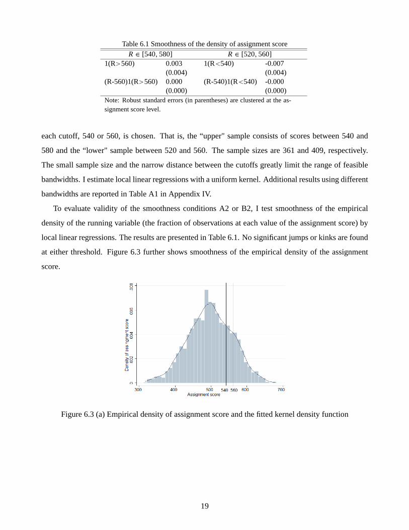
Table 6.1 Smoothness of the density of assignment score

R ∈ [540, 580] R ∈ [520, 560]

1(R>560) 0.003 1(R<540) -0.007

(0.004) (0.004)

(R-560)1(R>560) 0.000 (R-540)1(R<540) -0.000

(0.000) (0.000)

Note: Robust standard errors (in parentheses) are clustered at the as-

signment score level.

each cutoff, 540 or 560, is chosen. That is, the “upper" sample consists of scores between 540 and

580 and the “lower" sample between 520 and 560. The sample sizes are 361 and 409, respectively.

The small sample size and the narrow distance between the cutoffs greatly limit the range of feasible

bandwidths. I estimate local linear regressions with a uniform kernel. Additional results using different

bandwidths are reported in Table A1 in Appendix IV.

To evaluate validity of the smoothness conditions A2 or B2, I test smoothness of the empirical

density of the running variable (the fraction of observations at each value of the assignment score) by

local linear regressions. The results are presented in Table 6.1. No significant jumps or kinks are found

at either threshold. Figure 6.3 further shows smoothness of the empirical density of the assignment

score.

Figure 6.3 (a) Empirical density of assignment score and the fitted kernel density function

19

Figure 6.3 (b) Frequency of assignment score, local polynomial fit, and 95% CI

I next evaluate whether the conditional means of pre-determined covariates are smooth at the thresh-

olds. This test can be seen as a falsification test. Following the standard practice, I test that treatment

has no false significant effects on these covariates. That is, I apply the RPJK estimator using the co-

variates as dependent variables. Among the 46 covariates, attending an elite school shows a weakly

significant impact only on one indicator (out of eight) for mother’s SES category. That is, the false

rejection rate is roughly 2 percent. These results suggest that the required smoothness is plausible in

this case. Monotonicity pertains to the interpretation of the identified effects and will be assessed after

presenting the estimated complier or marginal complier characteristics.

Table 6.2 Complier or marginal complier characteristics

Age (months) Birth order Test7 Test9 High SES Middle SES Low SES

Upper threshold: R=560

123.5 2.490 115.7 119.4 0.098 0.567 0.335

(3.968)*** (0.420)*** (4.190)*** (3.161)*** (0.091) (0.132)*** (0.140)**

Lower threshold: R=540

124.1 1.778 121.1 123.8 0.230 0.467 0.304

(2.747)*** (0.183)*** (1.510)*** (1.887)*** (0.071)*** (0.062)*** (0.046)***

Note: Robust standard errors are clustered at each integer test score value; Age refers to that in

Dec. 1962; Test7 is test score at age 7 and test9 is test score at age 9; high SES refers to father in

professional or technical etc. non-manual occupation; Middle SES refers to father in skilled manual

profession; Low SES refers to father in unskilled, semiskilled profession or unemployed, disabled,

etc. **Significant at the 5% level; ***Significant at the 1% level.

Who are compliers or marginal compliers at the lower or upper kink points?16 Table 6.2 presents

16If the head teacher is the decision maker, then marginal compliers are those who the head teacher is indifferent to the

choices of assigning to an elite school or not. Put it differently, marginal compliers are the last (marginal) students the head

teacher would assign to an elite school if they scored just above the threshold, and would not otherwise.

20

the estimated average characteristics for compliers or marginal compliers. These characteristics in-

clude age in December 1962, birth order, test scores at age 7 and age 9, and SES in three categories.17

Compliers or marginal compliers at the lower kink point on average show more advantageous charac-

teristics than those at the upper kink point. For example, those at the upper threshold have lower test

scores at age 7 and age 9. They are less likely to be from a high SES family and more likely to be

from a middle SES family. They are also slightly younger and have a higher birth order. These results

might appear to be counter-intuitive. However, recall that at the lower threshold compliers or marginal

compliers only need to be just above the lower threshold to attend an elite school, while at the upper

threshold, they need to above the higher threshold to attend an elite school and would not otherwise.

Therefore, it is plausible that there is a positive selection into compliers or marginal compliers at the

lower threshold, and a negative selection at the upper threshold.

Table 6.3 First-stage and reduced-form outcome estimates

Dependent var. Elite

school

Elite

school

Education Education

R ∈ [540, 580]

1(R>560) 0.074 0.089 -0.050 -0.045

(0.057) (0.065) (0.478) (0.555)

(R-560)1(R>560) -0.044*** -0.043*** -0.077** -0.066*

(0.004) (0.005) (0.035) (0.038)

Covariates N Y N Y

R-squared 0.549 0.622 0.086 0.283

R ∈ [520, 560]

1(R<540) 0.098** 0.111** 0.689* 0.968**

(0.044) (0.047) (0.361) (0.412)

(R-540)1(R<540) -0.046*** -0.044*** -0.062** -0.059*

(0.004) (0.004) (0.029) (0.032)

Covariates N Y N Y

R-squared 0.439 0.524 0.053 0.259

Note: All specifications control for a linear term of the assignment score,

with or without additionally an extensive set of covariates, including fixed

effects for the school and grade attended in 1962, father’s social class in

eight categories, mother’s occupation in nine categories, age within grade,

and linear and quadratic terms of test scores at ages 7 and 9. Robust standard

errors are in parentheses and are clustered at the assignment score level; *

Significant at the 10% level; **Significant at the 5% level; ***Significant

at the 1% level.

The estimated complier or marginal complier characteristics all have the plausible positive sign and

all estimated probabilities are between 0 and 1. Formal one-sided tests cannot reject that the estimated

17These high, middle, and low SES indicators are constructed from the eight father’s social classes with some similar

adjacent categories combined.

21

mean characteristics are positive and that the probabilities are between 0 and 1 at any conventional

significance level. Overall, no evidence against monotonicity is found.

Table 6.3 presents estimation results from the first-stage and reduced-form outcome regressions.

Consistent with Figure 6.1, these estimates suggest that the probability of attending an elite school

has significant kinks at both thresholds, no significant jump at the upper threshold, and a somewhat

imprecisely estimated jump of 10 to 11 percent at the lower threshold. The estimated jumps and kinks

remain very similar regardless of whether one controls for the extensive set of covariates or not. This

is what one would expect if the design is valid.

Estimation of the reduced-form outcome equation reveals a similar pattern to the first-stage. For

example, at the upper threshold, both the first-stage and the reduced-from outcome estimates show

no significant jumps. Joint tests (provided in Table A2 in Appendix IV) further confirm that these

estimated jumps are jointly insignificant at the upper threshold, with or without including covariates.

If there were no jump in the first-stage, but a significant jump in the reduced-form outcome regression,

one would then be concerned about the validity of the monotonicity or smoothness assumptions.

Table 6.4 Impacts of elite school attendance on years of post-secondary education for males

RD RPK RPJK

R ∈ [540, 580]

-0.678 -0.509 1.735** 1.546* 1.703** 1.503*

(6.330) (5.709) (0.805) (0.824) (0.853) (0.888)

Covariates N Y N Y N Y

R ∈ [520, 560]

6.995 8.696* 1.335** 1.332** 1.536** 1.705**

(4.563) (4.516) (0.604) (0.646) (0.647) (0.731)

Covariates N Y N Y N Y

Note: The covariates included are fixed effects for the school and grade attended in

1962, father’s social class in eight categories, mother’s occupation in nine categories,

age within grade, and linear and quadratic terms of test scores at ages 7 and 9. Ro-

bust standard errors are clustered at the assignment score level and are in parentheses;

*Significant at the 10% level; **Significant at the 5% level.

Table 6.4 presents the estimated impacts of attending an elite school on educational attainment. In

the following I focus on estimates when controlling for the extensive set of covariates, though results

are largely robust to controlling for covariates or not. At the upper threshold, the jump is insignificant.

Consequently, the standard RD estimator leads to estimates with much larger standard errors and an

economically implausible negative sign. In contrast, the RPK estimator generates an estimated effect of

about 1.5 years, which is significant at the 5% level, so attending an elite school increases completed

22

post-secondary education by 1.5 years for males. The RPJK estimator generates estimates close to

those of the RPK estimator. This is consistent with Theorem 3 and Corollary 1b in that the 2SLS

estimator using both a jump and a kink as IVs reduces to the kink estimator when there is no jump.

At the lower threshold, the jump is significant at the 5% level. Recall that when a jump exists, the

RPK estimator is biased even with large samples, unless τ ′ (r0) equals 0. Based on equation (9), the

bias in the kink estimator equals τ ′ (r0) (P+− P−)/(P′+− P ′−). Here the jump appears to be much less

precisely estimated than the kink, having a standard error that is an order of magnitude larger than the

standard error of the kink estimate (see Table 6.4). So unless the bias in the kink estimator is very large,

estimation based on the kink will be much more accurate than the jump estimator, at least in terms of

root mean squared error (RMSE). The bias in the kink estimator is likely to be very small, both because

P ′+ − P ′− is relatively quite large (this is visible in Figure 6.2) and because τ ′ (r0) (P+ − P−) is likely

to be quite small.

To evaluate the possible bias in the RPK estimator, I formally test τ ′ (r0) (P+ − P−) = 0. Under

the null hypothesis that either τ ′ (r0) = 0 or (P+ − P−) = 0, the kink estimator is valid. I estimate

τ ′ (r0) (P+ − P−) using τ ′ (r0) (P+ − P−) = G ′+ − G ′− − τ(P ′+ − P ′−

)from equation (9), where

G ′+ − G ′− and P ′+ − P ′− are obtained from the slope changes in the reduced-form outcome and first-

stage treatment equations, respectively, and τ is estimated by the RPJK estimator. Estimating τ by the

RPJK estimator is valid under the null. It is also preferred because the standard RD estimator yields

largely misleading estimates of τ , as shown in the first two columns of Table 6.5.

Table 6.5 Biases in the kink estimator

R ∈ [540, 580] R ∈ [520, 560]

0.001 0.001 -0.008 -0.008

(0.010) (0.009) (0.010) (0.009)

Covariates N Y N Y

Note: Bootstrapped standard errors are based on 1,000 simulations.

Table 6.5 presents estimates of τ ′ (r0) (P+ − P−). For both the upper and lower samples, the

estimates are both numerically very small and are statistically insignificant, regardless of whether one

controls for covariates or not. These results strongly suggest that, by greatly decreasing variance while

adding little bias, the RPJK estimator provides a much more accurate estimate of the treatment effect

than the jump estimator at the lower threshold R = 540, despite the possible presence of a nonzero

jump there. The improved efficiency is particularly evident from the much smaller standard errors

or larger t statistics for the RPK and RPJK estimators. At the lower threshold, the RPK and RPJK

23

estimators produce estimates close to the estimates at the upper threshold. This is in sharp contrast to

the implausibly large positive estimates of 7 to over 8 years produced by the standard RD estimator.

Table A1 in Appendix IV provides additional results extending the lower assignment score sample

to be between 450 and 560 and the upper assignment score sample to be between 540 and 650. Again

it is clear that the RPK estimator and the RPJK estimator produce estimates reasonably close to those

reported in Table 6.2, while the standard RD estimator yields estimates either with an improbable

negative sign or implausibly large.

These nonparametric local analyses generally confirm the global parametric results in Clark and

Del Bono (2016). Their results were based on a constant treatment effect assumption. The results here

support that assumption, since similar treatment effects are found at each of the two thresholds, and

both local estimates are comparable to those obtained by Clark and Del Bono (2016). Taken together,

the empirical estimates above strongly support the theoretical results derived earlier. Specifically, these

estimates show that, in practice, one only needs to implement the RPJK estimator when the treatment

probability shows a relatively large kink and a small jump.

7 Military Service, Educational Attainment, and Earnings

This section presents a new empirical application and investigates program impacts in a different set-

ting. More than 60 countries around the world have mandatory military conscription.18 Conscription

typically either ends or interrupts an otherwise continuous educational path. Young men are usually

drafted at an important age for education. For example, the official conscription age in Russia is 18.

In addition, military service delays entry into the labor market, and shortens the lifetime over which

one can accumulate returns to (nonmilitary) human capital investments. Both effects may depress the

demand for higher education among conscripts.

Despite this expected reduction in the demand for higher education, the prevailing evidence from

the US and other OECD countries is that conscription increases college education. This increase has

been attributed to draft avoidance behavior (going to college to defer or avoid military service) or, in

the US, veterans obtaining additional education using subsidies provided by the G.I. bill. Leading work

documenting the former explanation includes Card and Lemieux (2011) and Bauer, Bender, Paloyo,

18A number of European countries have recently abolished it (France in 1996, Italy in 2005, Sweden in 2010, and

Germany in 2011).

24

and Schmidt (2011). The latter is discussed in Angrist and Chen (2011) as well as Bound and Turner

(2002).

Below I show that, contrary to the prevailing evidence in the US and other OECD countries, con-

scription in Russia causes a significance decrease in college education. Such a decrease is consistent

with the special circumstances of Russia. In particular, Russia did not have institutions comparable to

the G.I. bill, and alternatives to going to college existed there for avoiding conscription, so draft eligi-

ble young men do not have to go to college in order to avoid being drafted. The institutional setting in

Russia resulted in what one would expect from economic theory regarding educational outcomes and

earnings when education is interrupted and entry into the labor force is delayed.

In order to obtain the causal effects of serving in the Russian army, I take advantage of the fact that,

due to the demilitarization process in Russia that began at the end of 1980s, there is a kinked profile

in the military induction rate across birth cohorts. This has been used in Card and Yakovlev (2014).

They apply a kink design to estimate the causal effects of serving in the Russian army on alcohol

consumption, cigarette smoking, and related health problems. Here I look at how the compulsory

military service affects educational outcomes and earnings.

Based on the institutional setting, it is not clear whether there is a jump or not in the induction rate

starting from a particular cohort onward. However, a kink in the induction rate is very likely, due to

demilitarization occurring gradually over time rather than all at once. Empirically it is shown that both

a kink and a small jump appear to be present, so the RPJK design is what I will focus on.

Let T be a binary indicator for serving in the Russian army. The running variable R is the month-

and-year when one turned 18, the official conscription age in Russia.19 Following Card and Yakovlev

(2014), the cutoff point is taken to be January 1989. So Z = {R ≤ r0} indicates whether one turned 18

before January 1989 or not.

The analysis draws on the phase II data of the Russia Longitudinal Monitoring Survey (RLMS).20

RLMS is a nationally-representative survey. At the time of writing, the phase II longitudinal data have

been collected annually (with two exceptions, 1997 and 1999) from 1994 to 2014. The data cover

about 4,000 households (about 10,000 individual respondents). Questions on military service were

asked in 5 waves, in years 2005 and 2011-2014. Given the longitudinal nature of the survey, one can

19All month and year of birth observations are centered at the mid-month, i.e., it is assumed that individuals were born

in the mid-month. This alleviates the potential bias caused by using a discrete running variable (Dong, 2015).20This is the Russia Longitudinal Monitoring survey, RLMS-HSE, conducted by Higher School of Economics and ZAO

“Demoscope” together with Carolina Population Center, University of North Carolina at Chapel Hill and the Institute of

Sociology RAS. (RLMS-HSE sites: http://www.cpc.unc.edu/projects/rlms-hse, http://www.hse.ru/org/hse/rlms).

25

track down military service status for other waves. Conscription in Russia then was supposed to a 24

months of mandatory military service for all male citizens aged 18 - 27.21 The majority of males served

in the military before age 23. Here I focus on male adults aged 30-60, allowing for time to complete

education. The analysis looks at completed education by 2014 (by which time the youngest cohort in

the analysis are in their 30’s).

Table 7.1 Summary Statistics

Served in army Not served in army

N Mean SD N Mean SD

Turned 18 after Jan, 1989 5,153 0.326 0.469 2,116 0.630 0.483

College or above 5,141 0.179 0.384 2,107 0.427 0.495

High School 5,141 0.749 0.433 2,107 0.468 0.499

Less than HS 5,141 0.072 0.258 2,107 0.105 0.306

Earnings last month 31,73 15.05 34.17 9,377 19.78 31.92

Note: The sample consists of male adults aged 30 - 60 from RLMS 1994-2014; education is

the highest education observed by the last survey (2014), while earnings are those observed

in all 23 survey (1994 - 2014).

Table 7.1 presents sample summary statistics. Those who turned 18 after January 1989 have a much

lower probability of serving in the army, less than 33% compared to 63% among those who turned 18

before January 1989. In addition, those who served in the army are much less likely to have a college

education and much more likely to have only a high school education. Serving in the army is also asso-

ciated with lower monthly earnings. However, one cannot interpret these simple correlations as causal

effects. The conscription procedure in Russia ordinarily consists of a medical exam by physicians to

determine a candidate’s fitness for military service, and a determination by the draft board as to whether

the candidate should be exempted from military service, given a deferral, or drafted. Conscripts are

officially positively selected on health status; however, men from disadvantageous backgrounds are

more likely to be enlisted, due to the prevalence of draft avoidance behavior of the rich.22

21The conscription periods each year are from October 1 through December 31 and from April 1 through June 30.22For example, men from wealthy families can pay bribes to members of draft boards or doctors to avoid being drafted.

See Lokshin and Yemtsov (2008) for discussion of draft avoidance behavior in Russia.

26

Figure 7.1 (a) Cohort profiles of college education (200 months bandwidth)

Figure 7.1 (b) Cohort profiles of college education (120 months bandwidth)

The top row of Figure 7.1(a) presents the cohort (month-year turning 18) profiles of serving in the

army and college education for males and females, separately. The bottom row shows the same profiles

27

but wider bins are used for cell means (so there are fewer dots) to facilitate showing the curvature of the

raw data along with 90% confidence intervals. The figures clearly show that the share of males serving

in the army has a dramatic decline (a slope change) just to the right of the cutoff (normalized to be 0).

One can also see a possible small discontinuity at the cutoff. Correspondingly, college education among

males shows a visible slope change in the opposite direction to that in the first-stage figure. There also

appears to be a less noticeable discontinuity at the cutoff (still in the opposite direction). In contrast,

college education among females shows only a slight slope change. Moreover, when looking closer to

the cutoff (i.e., using a smaller bandwidth), the slope change among females starts to disappear.

Figure 7.1(b) presents the same plots as those in Figure 7.1(a), but uses a smaller bandwidth (120

months instead of 200 months on either side of the cutoff). There is little if any slope change for female

college education around the cutoff. In theory, a small kink for both men and women is possible due

to macro changes occurring at the time.23 I therefore use females as a control group in the main

analysis.This follows Card and Lemieux (2011), who use trends in the schooling of men relative to

those of women to measure draft effects. This strategy was also adopted by Card and Yakovlev (2014)

to measure the draft effects on alcohol consumption and cigarette smoking.

Table 7.2 Smoothness Tests

R=[-200, 199] R=[-120,119]

Density of running var.

Jump -5.269 (3.628) -4.650 (4.230)

Kink -0.139 (0.094) 0.084 (0.177)

Covariates

Father college education 0.087 (0.073) -0.004 (0.109)

Mother college education 0.128 (0.086) 0.043 (0.140)

Note: Estimates are based on RLMS 1994-2014; the density tests use a

regression of the frequency of observations at each value of the running

variable on Z , Z(R − r0), (R − r0), and (R − r0)2, where standard errors

are clustered at each value of the running variable; Covariate tests use the

same RPJK specification as the main specification for college education,

controlling for region fixed effects and region center fixed effects; Robust

standard errors are clustered at gender by month-year of birth level.

I first verify the smoothness conditions required for the RPJK estimator. Figure 7.2 provides visual

evidence showing smoothness of the empirical density of birth cohort (date turning 18). Table 7.2

presents formal test results. No significant jumps and kinks are found in the empirical density of birth

23For example, after the collapse of the Soviet Union, the number of higher education institutions in Russia increased

due to the emergence of private institutions, as well as greater enrollment of tuition paying students in public universities.

28

cohort. Falsification tests on the two directly relevant covariates for the outcomes of interest, mother’s

and father’s college education show insignificant treatment effects.24 Monotonicity is discussed after

presenting the estimated characteristics of compliers.

Figure 7.2 Frequency of birth cohort, local polynomial fit, and 95% CI

Who no longer joined the Russian Army due to the advent of demilitarization? Table 7.3 presents

the estimated average complier or marginal complier characteristics, including family size, mother

having a college education, father having a college education, living in a regional center, and living in

Moscow or St. Petersburg. Note that these two cities had much lower draft quotas than other places

(Lokshin and Yemtsov, 2008). Compliers in this case are those who would serve in the military if and

only if they were born before demilitarization but would not otherwise. These mean characteristics

are estimated by the approach discussed in Section 5. For comparison purposes, also reported are the

average characteristics of never takers and always takers.25 Never takers broadly consist of two distinct

types, 1) those who were ineligible (due to, e.g., real disability) even before the demilitarization, and

2) those who would avoid conscription regardless. For example, it is well known that those who live

in larger cities have better access to information and greater career opportunities and hence a higher

chance of avoiding being drafted. There is also evidence that those who are from smaller families are

more likely to avoid the draft (Lokshin and Yemtsov, 2008).

Indeed, estimates in Table 7.3 show that never takers are more likely to live in a regional center, to

24College education is coded as 1 if a father or mother has any education from a technical community college, medical

institute, university, academy, or taking a post-graduate course, and 0 otherwise.

25The average characteristics of never takers are identified as E [X |N , R = r0] =limr↓r0

E[XT |R=r ]

limr↓r0E[T R=r ]

and those of always

takers are identified as E [X |A, R = r0] =limr↑r0

E[X(1−T )T |R=r ]

limr↑r0E[1−T |R=r ]

.

29

Table 7.3 Complier, never taker, and always taker characteristics

Region

center

Moscow/St

Peters-

burg

Family

size

Father

college edu.

Mother

college

edu.

Complier 0.378 0.106 4.305 0.165 0.248

(0.009)*** (0.005)*** (0.028)*** (0.006)*** (0.008)***

Never taker 0.499 0.171 4.002 0.245 0.318

(0.041)*** (0.030)*** (0.129)*** (0.035)*** (0.036)***

Always taker 0.400 0.112 4.446 0.228 0.333

(0.015)*** (0.009)*** (0.053)*** (0.012)*** (0.014)***

Note: Estimates are based on RLMS 1994-2014; Moscow means whether the respondent lives

in Moscow city or St. Petersburg; Robust standard errors are clustered at year-month of birth

level; ***Significant at the 1% level.

be from Moscow or St. Petersburg, and to come from smaller families. Note that selection on parental

education for never takers can go in either direction, depending on the specific reasons they did not

serve in the military. In contrast, compliers are slightly less likely to live in a regional center or live in

Moscow or St. Petersburg. They on average are from slightly larger families and are less likely to have

college educated parents. Overall it looks like those who no longer joined the Russian Army thanks

to the start of demilitarization are those from average family backgrounds, having mean characteristics

comparable to the sample means of those who served in the military.

These estimated complier characteristics all carry the plausible positive signs; the estimated proba-

bilities are well between 0 and 1. Formal one-sided tests fail to reject that the mean characteristics are

positive or the probabilities are between 0 and 1. Therefore, monotonicity is not rejected.

Table 7.4 reports the 2SLS estimates of the impact of military service on college education. Also

reported are the estimated jump and kink in the first-stage. Considering that macro changes other than

demilitarization or simply specification errors may lead to kinks in the probability of college education,

I use females as a control group. The underlying assumption is that any macro changes or specification

errors would lead to the same trend changes for males and females.26

The top panel of Table 7.4 reports estimates using a bandwidth of 200 months on either side of

the cutoff (corresponding to Figure 7.1(a)) and the bottom panel reports estimates using a smaller

bandwidth of 120 months (corresponding to Figure 7.1(b)). As expected, estimates in the top panel are

26In particular, I estimate a regression of college education Y on T , (R − r0), Z , Z(R− r0), male, and male× (R− r0),using either the jump male × Z or the kink male × Z × (R − r0), or both in the male probability of serving in the army,

as the excluded IVs for T . Essentially, the jump and kink in the numerator of the RPJK estimator are the male-female

differences.

30

Table 7.4 Impacts of serving in the army on college education

First-stage 2SLS estimates

Jump Kink RD RPK RPJK

R=[-200,199]

0.094 0.002 0.045 -0.184 -0.145

(0.022)*** (0.000)*** (0.202) (0.081)** (0.070)**

R=[-120,119]

0.114 0.003 -0.180 -0.281 -0.256

(0.026)*** (0.000)*** (0.201) (0.126)** (0.111)**

Note: Estimates are based on RLMS 1994-2014; All estimates use fe-

males as a control group, and additionally control for region fixed ef-

fects for 39 regions, regional center fixed effect, and father’s education

and mother’s education in 12 categories each; Robust standard errors

are clustered at gender by month-year of birth level; **Significant at

the 5% level; ***Significant at the 1% level.

in general more precise due to a larger sample size, and hence are what I will focus on in the following

discussion. Both the estimated jump and kink in the first-stage are statistically significant. However,

the jump appears to be too small to yield precise estimates of the effects of military service. In contrast,

the RPJK design yields significant negative impacts. In the top row, serving in the army is shown to

reduce a male adult’s probability of obtaining a college education by about 14.5%. The RPK design

yields similar negative effects. Estimates using only males are provided in Table A3 in Appendix V.

Using only the male sample generally overestimates the impacts of serving in the army.

Figure 7.3 Estimated impacts on college education with different bandwidths

Figure 7.3 further plots estimates over a large range of bandwidths along with the 90% confidence

intervals. The RPJK and RPK designs yield statistically significant negative estimates that are stable

over a large range of bandwidths (though, not surprisingly, estimates become insignificant when very

small bandwidths are used). In contrast, the standard RD design generates estimates that are never

significant.

31

To corroborate the estimated significant negative impacts on college education, I conduct a falsi-

fication analysis. Serving in the army interferes with the transition from high school to college, but

should rarely if ever interfere with the opportunity of obtaining a less than high-school education. Ta-

ble 7.5 presents results for less than high school education, using the same specifications as those used

for college education. The estimated jump and kink in the first-stage are the same, while the estimated

impacts on less than high education are small and positive yet insignificant in all cases.

Table 7.5 Impacts of serving in the army on less than high school education

First-stage 2SLS estimates

Jump Kink RD RPK RPJK

R=[-200,199]

0.094 0.002 0.037 0.044 0.043

(0.022)*** (0.000)*** (0.140) (0.059) (0.050)

R=[-120,119]

0.114 0.003 0.053 0.097 0.037

(0.026)*** (0.000)*** (0.140) (0.085) (0.140)

Note: Estimates are based on RLMS 1994-2014; All estimates use fe-

males as a control group, and additionally control for region fixed ef-

fects, regional center fixed effect, and father’s education and mother’s

education dummies; Robust standard errors are clustered at gender by

month-year of birth level; ***Significant at the 1% level.

Unlike some evidence from the US and other OECD countries, the above analysis shows that serv-

ing in the army significantly decreases one’s probability of obtaining a college degree in Russia. This

is what one would expect from economic theory when education is interrupted and entry into the labor

force is delayed. In particular, Russia does not provide financial support for higher education to re-

turning conscripts. Also, attending college may not be the primary means of avoiding being drafted in

Russia, since illegitimate (arguably less expensive) alternatives are prevalent.27,28 Assume that at least

some eligible draftees avoid being drafted through attending college. Then the estimates here would

be underestimates for the true interruption impact of compulsory military service on higher education.

27According to the General Staff of the Armed Forces, every year approximately 30,000 young men dodge the draft. As

a result, Less than 10 percent of eligible males were actually enlisted in the army in the early 2000s.28Spivak and Pridemore (2014) note that of the three primary grounds upon which conscription can be exempted, ed-

ucational deferment, certain social hardships, and medical disqualification, the latter is the most commonly exploited. In

addition, simply evading the draft is prevalent.

32

Figure 7.4 (a) Cohort profiles of earnings (200 months bandwidth)

Figure 7.4 (b) Cohort profiles of earnings (120 months bandwidth)

I next investigate whether conscription leads to lower earnings, given its negative impacts on higher

education. Figure 7.4 (a) presents the birth cohort profiles of monthly earnings (total income in the last

33

30 days) for males and females, respectively. All earnings are in 2014 constant thousands of Rubles.

Unlike completed education, earnings are not time invariant. Longitudinal data are then used for these

figures as well as for the estimation. The first-stage figure now using the longitudinal data similarly

shows a dramatic slope change and a small jump in the probability of serving in the Russian army in

January 1989.

Table 7.6 Impacts of serving in the army on earnings

First-stage 2SLS estimates

Jump Kink RD RPK RPJK

R=[-200,199]

0.072 0.002 17.37 -10.91 -6.117

(0.026)*** (0.000)*** (13.54) (3.718)*** (3.389)*

R=[-120,119]

0.107 0.003 10.08 -12.06 -6.126

(0.031)*** (0.000)*** (98.46) (5.444)** (4.596)

Note: Estimates are based on RLMS 2000-2014; All estimates use fe-

males as a control group, and additionally control for region fixed ef-

fects, regional center fixed effect, and father’s education and mother’s

education dummies; Robust standard errors are clustered at gender by

month-year of birth level; * Significant at the 10% level; **Significant

at the 5% level; ***Significant at the 1% level.

Table 7.6 presents results for earnings by the RD, RPK, and RPJK designs. These results are pro-

duced by the same specifications as those for college education, except that due to the longitudinal

nature, I additionally control for year fixed effects as well as age and age squared. The standard RD

design yields positive and insignificant estimates. In contrast, the RPJK design yields a significant

estimate of -6.117 thousands of Rubles (about 95 USD, or roughly a 30 percent decrease in reference

to the mean earnings of those who do not serve in the army). The RPK design with the 200 months

bandwidth yields a negative effect of -10.91 thousands of Rubles (about 170 USD). Using the smaller

bandwidth leads to similar but less precise estimates. Only data from 2000 or later are used for es-

timates in Table 7.5, because the labor market in the 1990’s in Russia went though many changes,

including the collapse of the Soviet Union. For comparison purposes, estimates using all years’ data

from 1994 to 2000 are provided in Table A4 in Appendix V. Interestingly, the estimates are largely

similar regardless of whether earlier years’ data are included or not, though precision is lower when

the noisier earlier years’ data are included.

34

Figure 7.5 Estimated impacts on college education with different bandwidths

Figure 7.5 further presents estimates with 90% confidence intervals over a wide range of band-

widths. The standard RD design yields estimates that are never significant and mostly positive. In

contrast, the RPJK and RPK designs yield negative and significant estimates for a large range of band-

widths. Overall these estimates point to negative effects of serving in the Russian army on earnings.

Estimates leaving out females as controls are provided in Table A5 in Appendix V. The conclusions

are similar except that the estimates are more sensitive to bandwidth choice.

Existing studies using the US or other OECD countries data show mixed evidence of conscription

on earnings, from positive, zero to negative impacts. These differences could be because conscription

experience varies greatly across countries. This variation is emphasized by Hjalmarsson and Lindquist

(2016). In countries like the US and OECD, where most studies find positive effects of conscription on

education, the resulting impacts on earnings could be offset by negative effects such as delayed entry

into the labor force. In contrast, I find large negative effects of conscription on earnings in Russia, likely

because military service in Russia reduces education, and so compounds rather than offsets negative

effects such as delayed entry into the labor force. Additional sources of negative effects on earnings

could be due to findings by Card and Yakovlev (2014), who show that compulsory military service in

Russia leads to significant increases in alcohol consumption and cigarette smoking as well as related

chronic health problems among conscripts. One caveat regarding these results is that, unlike completed

education, gender differences in earnings might be more sensitive to labor market changes and hence

it is not clear that women provide as good a control group as the case of college education.

In situations where a significant jump in the conscription probability across birth cohorts exists,

e.g., when compulsory military service is either introduced or abolished, one may apply the standard

RD design (see, e.g., Bauer, Bender, Paloyo, and Schmidt 2011 and references therein). However,

when one is unsure if jumps are present or large enough to strongly identify treatment effects, as in

35

the case of Russia, the above results illustrate the advantage of the RPJK design over the standard RD

design.

8 Conclusion

This paper evaluates the impacts of participation in two social programs, elite school attendance in the

UK and supposedly compulsory military service in Russia. In both cases, the probability of participa-

tion has large kinks but either a small jump or no jump. As a result, evaluating the program impacts

is largely impossible using the standard RD estimator. This paper extends the standard RD design

with a binary treatment to allow for causal identification in these or similar scenarios. In particular, I

discuss identifying causal parameters using a kink, instead of or in addition to a jump, in the treatment

probability at a policy threshold.

Kinks in the treatment probability can frequently arise, as when the assignment of treatment de-

pends on how far one is from the cutoff. Kinks can also arise due to kinked benefit or cost schedules

that affect individuals treatment decisions. Similar to the standard RD design, identification based on

kinks is valid under smoothness conditions. These smoothness conditions are plausible when individ-

uals cannot sort around the kink point by precisely manipulating the running variable. To empirically

check validity of these smoothness conditions, one can test smoothness (i.e., no jumps and kinks) of

the empirical density of the running variable, or the conditional means of pre-determined covariates.

This paper focuses on identification. Robust nonparametric inference for the resulting RPK estima-

tor is discussed in Calonico, Cattaneo, and Titiunik (2014). In addition, Chiang, Hsu, and Sasaki (2017)

discuss bootstrap validity a class of discontinuity based estimators that includes the RPK estimator.

In practice, treatment probabilities may show both a jump and a kink at the RD threshold. This

paper then discusses a general RPJK design that is valid regardless of whether there is either a jump,

a kink or both. The corresponding local 2SLS estimator asymptotically reduces to the standard RD

estimator when a jump is present in the treatment probability, and otherwise reduces to the newly pro-

posed PRK estimator if there is no jump. Higher order nonsmoothness, like a second-order derivative

change, could also be exploited using methods similar to the RPK and RPJK designs.

Additional identification results, such as identifying complier or marginal complier characteristics

in the RD, RPK, and RPJK designs, are also discussed. Identifying complier or marginal complier

characteristics provides a convenient way of checking for monotonicity in empirical applications.

36

In sharp contrast to the results of the standard RD design, the proposed RPK or RPJK designs

yield plausible estimates of causal impacts of the two social programs under consideration. Attending

an elite school in the UK is estimated to increase education by 1.3-1.5 years for men. Serving in the

Russian army decreases the probability of obtaining a college education by 14.5 percent among men.

It is worth mentioning that this paper discusses identification in a static model. This is similar

to the standard RD design. When the running variable is time, kinks in outcomes may result from

dynamic effects, such as variable delays in response to treatment. Extending the results in this paper to

a dynamic context would be an interesting direction for future research.

9 Appendix I: Proofs

PROOF of THEOREM 1: The conclusion follows by the derivation in the text.

PROOF of THEOREM 2: For r ≥ r0,

G(r) ≡ E[Y0 + (Y 1−Y 0)T |R = r

]= E

[Y0 + (Y 1−Y 0)T 1|R = r

]= E [Y0|R = r, T1 = 0] Pr (T1= 0|R = r)+ E [Y1|R = r, T1 = 1] Pr (T1= 1|R = r)

= E [Y0|R = r, N ] Pr (N |R = r)+ E [Y1|R = r, A] Pr (A|R = r)+ E [Y1|R = r,C] Pr (C |R = r) ,

where the first equality follows from the fact that for r ≥ r0, T = T1, and the last equality follows from

the monotonicity assumption B1.

Similarly for r < r0,

G(r) ≡ E[Y0 + (Y 1−Y 0)T |R = r

]= E

[Y0 + (Y 1−Y 0)T 0|R = r

]= E [Y0|R = r, T0 = 0] Pr (T0= 0|R = r)+ E [Y1|R = r, T0 = 1] Pr (T0= 1|R = r)

= E [Y0|R = r, N ] Pr (N |R = r)+ E [Y1|R = r, A] Pr (A|R = r)+ E [Y0|R = r,C] Pr (C |R = r) .

Under B2, the probabilities of types and type-specific conditional means of potential outcomes are

continuously differentiable. Therefore, any terms for always takers and never takers will be differenced

37

out in the following derivation. Then

G+ − G− = E [Y1|R = r0,C] Pr (C |R = r)− E [Y0|R = r0,C] Pr (C |R = r0)

= E [Y1 − Y0|R = r0,C] Pr (C |R = r0)

= τ (r0)Pr (C |R = r0) ,

where τ (r0) ≡ E [Y1 − Y0|R = r0,C]. The equivalent definition in Section 2.1 is τ (r0) = τ L AT E (P+, P−, r0) ≡

E[Y1 − Y0|R = r, P−< U ≤ P+

].

Similarly,

P+ − P− = limr↓r0

E [T |R = r ]− limr↑r0

E [T |R = r ] = Pr [C |R = r0] .

Further,

G ′+ − G ′− = limr↓r0

{∂∂r

E [Y1|R =r ,C (r)] Pr (C |R = r)+E [Y1|R = r,C (r)] ∂∂r

Pr (C (r) |R = r)}

− limr↑r0

{∂∂r

E [Y0|R =r ,C (r)] Pr (C (r) |R = r)−E [Y0|R = r0,C (r)] ∂∂r

Pr (C (r) |R = r)}

= ∂∂r

E [Y1 − Y0|R =r ,C (r)] |r0Pr (C (r) |R = r0)+ E [Y1 − Y0|R = r0,C (r0)]

∂∂r

Pr (C (r) |R = r) |r0.

It follows that

G ′+ − G ′− = τ′ (r0)Pr (C (r) |R = r0)+ τ (r0)

∂

∂rPr (C (r) |R = r) |r0

,

where τ ′ (r0) ≡∂∂r

E [Y1 − Y0|R = r,C (r)] |r0. The equivalent definition in Section 2.1 is τ ′ (r0) ≡

∂∂rτ (r) |r0

≡ ∂∂r

E [Y1 − Y0|R = r, P0 (r)< U ≤ P1 (r)] |r0. Similarly,

P ′+ − P ′− =∂

∂rPr (C (r) |R = r) |r0

.

Since Pr (C (r) |R = r0) = P+ − P−, then

G ′+ − G ′− = τ′ (r0) (P+ − P−)+ τ (r0)

(P ′+ − P ′−

). (18)

When the jump P+ − P− goes arbitrarily to 0, τ (r0) = τ L AT E (P+, P−, r0) goes arbitrarily to

τMT E (P (r0)). Further by the above equation (18), when there is a kink, P ′+− P ′− 6= 0, τMT E (P (r0))

38

is identified by τMT E (P (r0)) =(G ′+ − G ′−

)/(P ′+ − P ′−

).

PROOF of THEOREM 3:

When there is a jump, ωn goes to zero as n→∞, and so equation (10) reduces to τ L AT E (P+, P−, r0) =

(G+ − G−) /(P+−P−), i.e., the standard RD estimand. When there is no jump, by assumption there is

a kink, then equation (10) reduces to τ L AT E (P+, P−, r0) = τMT E (P (r0)) =(G ′+ − G ′−

)/(P ′+ − P ′−

),

the PRK estimand, which is valid by Theorem 1 or 2.

PROOF of COROLLARIES 1a and 1b:

By equation (2), τ L AT E (P+, P−, r0) = (G+ − G−) /(P+ − P−). By equation (9), G ′+ − G ′− =

τ ′ (r0) (P+ − P−) + τ (r0)(P ′+ − P ′−

), where recall τ (r0) ≡ τ L AT E (P+, P−, r0). Then when P+ −

P− 6= 0, if and only if τ ′ (r0) = 0, G ′+−G ′− = τ (r0)(P ′+ − P ′−

)and hence τ (r0) =

(G ′+ − G ′−

)/(P ′+ − P ′−

).

That is, when τ ′ (r0) = 0, a jump and a kink identify the same parameter. This proves Corollary 1a

τ L AT E (P+, P−, r0) =G+ − G−

P+ − P−=

G ′+ − G ′−

P ′+ − P ′−.

It follows that (G+ − G−) = (P+ − P−) τ L AT E (P+, P−, r0) and(G ′+ − G ′−

)=(P ′+ − P ′−

)τ L AT E (P+, P−, r0).

One can then take a linear combination of the jump and kink on both sides: G+−G−+ω(G ′+ − G ′−

)=(

(P+ − P−)+ ω(P ′+ − P ′−

))τ L AT E (P+, P−, r0) for any weights ω 6= − (P+ − P−) /

(P ′+ − P ′−

).

Then

τ L AT E (P+, P−, r0) =G+ − G− + ω

(G ′+ − G ′−

)P+ − P− + ω

(P ′+ − P ′−

) .

for ω 6= − (P+ − P−) /(P ′+ − P ′−

). The above holds when either P+ − P− 6= 0, or P ′+ − P ′− 6= 0, or

both, which proves Corollary 1b.

10 Appendix II: Identifying Other Parameters of Interest

Define Gt (r) ≡ E [1 (T = t) Y |R = r ] for t = 0, 1. Follow the notational convention to let Gt+ and

Gt− be the right and left limits and G′t+and G′t− be the right and left derivatives at r = r0, respectively,

whenever they exist.

Corollary 2 Assume that A1 holds and that A2 hold holds after replacing E [Yt |U = u, R = r ] with

FYt |U,R (y|u, r), t = 0, 1. 1) If P+ 6= P−, then E[Yt |P− < U ≤ P+, R = r0

]= Gt+−Gt−

P+−P−; 2) if P+ =

39

P− and P ′+ 6= −P ′−, then E [Yt |U = P (r0) , R = r0] =G′t+−G′t−P ′+−P ′−

; 3) Assume A3 holds. If P+ = P−

and P ′+ = P ′− do not both hold, then E[Yt |P− < U ≤ P+, R = r0

]= limn→∞

(Gt+−Gt−)+$ n(G′t+−G′t−)P+−P−+$ n(P+−P−)

,

where $ n → 0 as n → ∞ and $ n can be the local 2SLS weights discussed in Section 4. Further

replacing Y with 1 (Y ≤ y) in the definiton of Gt (r), one can identify FYt |P−<U≤P+,R=r0(y).

PROOF OF COROLLARY 2: Part 1) is the standard RD design estimand. This result can be

proved by following, e.g., the identification results of Frandsen, Frölich, and Melly (2012). Part 3) can

be readily proved by following the arguments in Theorem 3 and the discussion in Section 3. Below I

provide a quick proof of part 2).

For t = 1, by definition

G′1+ − G′1− = limr↓r0

∂

∂rE [T Y |R = r ]− lim

r↑r0

∂

∂rE [T Y |R = r ]

= limr↓r0

∂

∂rE [T Y1|R = r ]− lim

r↑r0

∂

∂rE [T Y1|R = r ]

= limr↓r0

∂

∂rE [1 (U ≤ P1 (r)) Y1|R = r ]− lim

r↑r0

∂

∂rE [1 (U ≤ P0 (r)) Y1|R = r ]

= limr↓r0

∂

∂r

∫ P1(r)

0

E [Y1|R = r,U = u] du − limr↑r0

∂

∂r

∫ P0(r)

0

E [Y1|R = r,U = u] du

= P ′+E[Y1|R = r0,U = P+

]− P ′−E

[Y1|R = r0,U = P−

]+

∫ P+

P−E [Y1|R = r,U = u] du

=(P ′+ − P ′−

)E [Y1|R = r0,U = P (r0)]

where the first to third equalities follow from the definition of Gt (r) for t = 0 and the equalities

Y = Y1T+Y0 (1− T ) and T = T1 Z+T0 (1− Z) for Z = 1 (r ≥ r0), and the last equality follows from

P+−P− = 0. By Theorem 1 and its proof, limr↓r0

∂∂r

E [T |R = r ]−limr↑r0

∂∂r

E [T |R = r ] = P ′+−P ′−.

It follows that

G′1+ − G′1−P ′+ − P ′−

=limr↓r0

∂∂r

E [T Y |R = r ]− limr↑r0

∂∂r

E [T Y |R = r ]

limr↓r0

∂∂r

E [T |R = r ]− limr↑r0

∂∂r

E [T |R = r ]

= E [Y1|R = r0,U = P (r0)] .

The case where t = 0 can be analogously proved.

Corollary 3 Assume that A1 holds and that A2 holds after replacing Yt , t = 0, 1 with some pre-

determined covariate X. 1) If P+ − P− 6= 0, then E[X |P− < U ≤ P+, R = r0

]= X+−X−

P+−P−; 2)

40

If P+ − P− = 0 and P ′+ − P ′− 6= 0, then E [X |U = P (r0) , R = r0] =X′+−X′−P ′+−P ′−

; 3) Assume A3

holds. If P+ − P− = 0 and P ′+ − P ′− = 0 do not both hold, then E[X |P− < U ≤ P+, R = r0

]=

limn→∞(X+−X−)+κn(X′+−X′−)(P+−P−)+κn(P ′+−P ′−)

, where κn → 0 as n → ∞ and κn can be the local 2SLS weights

discussed in Section 4. Further replacing X with 1 (X ≤ x) in the definiton of X (r), one can identify

FX |P−<U≤P+,R=r0(x).

PROOF OF COROLLARY 3: Recall X (r) ≡ E [XT |R = r ]. This corollary can be proved anal-

ogously to the proof of Corollary 2 by replacing 1(T = 1)Y with XT or 1(T = 1)1 (Y ≤ y) with

1 (X ≤ x) T and noticing that X does not change with T = t , t = 0, 1.

11 Appendix III: Identification Using Higher-order Derivative Changes

The estimand in Corollary 1b requires τ ′ (r0) = 0 to use both a jump and a kink for identification. As

mentioned, having τ ′ (r0) = 0 means that the treatment effect does not vary linearly with the running

variable R.

The following Corollary 4 provides extensions of Corollary 1b to allow τ ′ (r0) 6= 0 while still

exploiting information in a kink in addition to a jump. For example, if the treatment is attending

an elite school, the running variable is test score, and the outcome is educational attainment, then

τ ′ (r0) 6= 0 would mean that the effect of attending an elite school on educational attainment depends

on the pre-treatment test score, and in this case one still could use both jump and kink information to

estimate the treatment effect.

For any function H (r), let H ′′+ and H ′′− be the right and left limits at r = r0 of its second derivative,

whenever they exist. For convenience of notation, formally define γ 1 ≡ G+ − G−, γ 2 ≡ G ′+ − G ′−,

γ 3 ≡ G ′′+ − G ′′−, β1 ≡ P+ − P−, β2 ≡ P ′+ − P ′− and β3 ≡ P ′′+ − P ′′−. So γ 1, γ 2, and γ 3 (β1, β2, and

β3) as the intercept, slope, and second-order derivative changes, respectively, of the conditional mean

function of the outcome (treatment) conditional on r at r = r0. Let τ ′′ (r0) ≡∂2

∂r2 τ (r) |r0, where recall

τ (r) ≡ τ L AT E (P1 (r) , P0 (r) , r) ≡ E [Y1 − Y0|P0 (r) ≤ U ≤ P1 (r) , R = r ].

Corollary 4 Assume that A1 holds. Further assume that all the funtions in A2 and A3 are continu-

ously twice differentiable. Assume that both P+ 6= P− and P ′+ 6= P ′−, and τ ′′ (r0) = 0. Then

τ L AT E (P+, P−, r0) =γ 1 + w

(2β2γ 2 − γ 3β1

)β1 + w

(2β2

2 − β3β1

) (19)

41

for any weights w 6= −β1/(2β2

2 − β3β1

).

Continuously twice differentiability and monotonicity imply that all the limits and derivatives in-

volved in the definitions of γ 1, γ 2, γ 3, β1, β2 and β3 exist.

Analogous to Corollary 1b, the assumption that τ ′′ (r0) = 0 in the above will hold if the treatment

effect is locally linear or locally constant. However, while a locally linear or constant treatment effect

is sufficient for τ ′′ (r0) = 0, it is stronger than necessary, because it implies that all derivatives higher

than the first are zero, instead of just the second derivative being zero. When τ ′′ (r0) = 0, Y cannot be

a nontrivial function of T (R − r0)2, but can be a function of T or T (R − r0) or both.

PROOF of COROLLARY 4:

By equation (18) G ′+ − G ′− = τ′ (r0) (P+ − P−)+ τ (r0)

(P ′+ − P ′−

). When Pz (r), z = 0, 1, and

E(Yt |U = u, R = r), t = 0, 1, are continuously twice differentiable in the neighborhood of r = r0.

Analogous to the derivation of equation (9), we have

G ′′+ − G ′′− = τ′′ (r0) (P+ − P−)+ 2τ ′ (r0) (P

′+ − P ′−)+ τ (r0)

(P ′′+ − P ′′−

).

The above along with G+ − G− = τ (r0) (P+ − P−) and equation (18) gives the following system

of equations:

G+ − G− = τ (r0) (P+ − P−),

G ′+ − G ′− = τ ′ (r0) (P+ − P−)+ τ (r0)(P ′+ − P ′−

),

G ′′+ − G ′′− = τ ′′ (r0) (P+ − P−)+ 2τ ′ (r0) (P′+ − P ′−)+ τ (r0)

(P ′′+ − P ′′−

).

Rewrite the above system of equations using notations defined in the text, we have

γ 1 = τ (r0) β1, γ 2 = τ′ (r0) β1 + τ (r0) β2, and γ 3 = τ

′′ (r0) β1 + 2τ ′ (r0) β2 + τ (r0) β3.

Given τ ′′ (r0) = 0, one can solve for τ (r0) from the second and third equation in the above to have

τ (r0) =(2β2γ 2 − γ 3β1

)/(2β2

2 − β3β1

). Given a jump we still have τ (r0) = γ 1/β1. By definition,

τ (r0) ≡ τ L AT E (P+, P−, r0). It then follows that

τ L AT E (P+, P−, r0) =γ 1

β1

=2β2γ 2 − γ 3β1

2β22 − β3β1

=γ 1 + w

(2β2γ 2 − γ 3β1

)β1 + w

(2β2

2 − β3β1

) ,

42

for any w 6= −β1/(2β2

2 − β3β1

).

Similar estimands can be constructed if the d-th derivative τ (d) (r0) = 0 for any finite positive

integer d, as is the case if the treatment effect is a polynomial of degree d−1 or less in (R−r0). In this

case, the treatment effect can be an arbitrarily high-order (e.g., up to the (d − 1)-th order) polynomial

of (R− r0), as long as the order is finite. Keep taking derivatives on both sides of γ 1 = τ (r0) β1, until

the d-th derivative. With the system of d equations and τ (d) (r0) = 0, one can back out τ (r0), as the

system of equations are recursive in nature.

12 Appendix IV: Additional Results (Elite School)

Table A1 Impacts of elite school attendance on post-compulsory education for males (alternative bandwidths)

RD RPK RPJK

R ∈ [540, 650]

-0.730 -0.416 1.571*** 1.582*** 1.335*** 1.343***

(3.547) (2.881) (0.442) (0.522) (0.413) (0.420)

Covariates N Y N Y N Y

R ∈ [450, 560]

4.100 4.495 1.663*** 1.719*** 1.364*** 1.378***

(3.492) (3.520) (0.422) (0.428) (0.349) (0.339)

Covariates N Y N Y N Y

Note: All specifications control for a linear term of the assignment score, with or without

additionally an extensive set of covariates, including fixed effects for the school and grade

attended in 1962, father’s social class in eight categories, mother’s occupation in nine cate-

gories, age within grade, and linear and quadratic terms of test scores at ages 7 and 9. Robust

standard errors are in parentheses and are clustered at the assignment score level; ***Signif-

icant at the 1% level.

Table A2 Joint test of the jumps in the first-stage and reduced-form outcome regressions for males

Lower threshold: R = 540 Upper threshold: R = 560

χ2(2) 8.22 11.6 1.76 2.23

P value (0.016) (0.003) (0.416) (0.327)

Covariates N Y N Y

N 409 409 361 361

43

Figure A1 Assignment score and elite school attendance for females

Figure A2 Assignment score and post-secondary education for females

Figure A3 (a) Density of assignment score (females)

44

Figure A3 (b) Frequency of assignment score, local polynomial fit, and 95% CI (females)

Table A3 Smoothness of the density of assignment score (females)

R ∈[540,580] R ∈[520,560]

1(R>560) 0.005 1(R<540) 0.004

(0.004) (0.005)

(R-560)1(R>560) -0.000 (R-540)1(R<540) -0.000

(0.001) (0.001)

Note: Robust standard errors are in parentheses.

Table A4 Complier or marginal complier characteristics (females)

Age (months) Birth order Test7 Test9 High SES Middle SES Low SES

Upper threshold: R=560

111.7 1.932 119.9 118 0.246 0.615 0.139

(4.506)*** (0.321)*** (5.767)*** (3.385)*** (0.113)** (0.131)*** (0.134)

Lower threshold: R=540

119.6 1.929 120 123.5 0.118 0.49 0.392

(1.841)*** (0.152)*** (2.015)*** (1.017)*** (0.072) (0.103)*** (0.072)***

Note: Robust standard errors are clustered at each integer test score value; Age refers to that in

Dec. 1962; Test7 is test score at age 7 and test9 is test score at age 9; high SES refers to father in

professional or technical etc. non-manual occupation; Middle SES refers to father in skilled manual

profession; Low SES refers to father in unskilled, semiskilled profession or unemployed, disabled,

etc. **Significant at the 5% level; ***Significant at the 1% level.

45

Table A5 First-stage and reduced-form outcome estimates for females

Dependent var. Elite

school

Elite

school

Education Education

R ∈[540,580]

1(R>560) 0.167*** 0.175*** -0.010 0.093

(0.059) (0.056) (0.416) (0.482)

(R-560)1(R>560) -0.033*** -0.031*** -0.084** -0.050

(0.005) (0.005) (0.036) (0.038)

Covariates N Y N Y

R-squared 0.546 0.604 0.029 0.202

R ∈[520,560]

1(R<540) 0.110* 0.091 0.026 -0.225

(0.056) (0.064) (0.263) (0.264)

(R-540)1(R<540) -0.039*** -0.039*** -0.046* -0.018

(0.004) (0.004) (0.023) (0.028)

Covariates N Y N Y

R-squared 0.368 0.440 0.069 0.252

Note: All specifications control for a linear term of the assignment score, with

or without additionally an extensive set of covariates, including fixed effects

for the school and grade attended in 1962, father’s social class in eight cate-

gories, mother’s occupation in nine categories, age within grade, and linear and

quadratic terms of test scores at ages 7 and 9. Robust standard errors are in

parentheses and are clustered at the assignment score level; * Significant at the

10% level; **Significant at the 5% level; ***Significant at the 1% level.

Table A6 Impacts of elite school attendance on years of post-secondary education for females

Jump Estimator Kink Estimator Jump&Kink Estimator

R ∈[540,580]

-0.062 0.532 2.560** 1.620 2.187* 1.427

(2.438) (2.592) (1.268) (1.229) (1.204) (1.204)

Covariates N Y N Y N

R ∈[520,560]

0.237 -2.468 1.176* 0.469 1.123* 0.365

(2.382) (2.850) (0.629) (0.674) (0.662) (0.699)

Covariates N Y N Y N

Note: The covariates included are fixed effects for the school and grade attended in 1962,

father’s social class in eight categories, mother’s occupation in nine categories, age within

grade, and linear and quadratic terms of test scores at ages 7 and 9. Robust standard errors

are clustered at the assignment score level and are in parentheses; *Significant at the 10%

level; **Significant at the 5% level.

Table A7 Biases in the kink estimator (females)

R ∈[540,580] R ∈ 520,560]

-0.010 -0.010 0.001 0.001

(0.017) (0.017) (0.006) (0.006)

Covariates N Y N Y

Note: Bootstrapped standard errors are based on 1,000 simulations.

46

13 Appendix V: Additional Results (Compulsory Military Service)

Table A8 Impacts of serving in the army on college education (males only)

First-stage 2SLS estimates

Jump Kink RD RPK RPJK

R ∈[-200,199]

0.091 0.002 0.171 -0.449 -0.353

(0.022)*** (0.000)*** (0.213) (0.088)*** (0.074)***

R ∈[-120,119]

0.114 0.003 -0.071 -0.421 -0.343

(0.026)*** (0.000)*** (0.197) (0.127)*** (0.111)***

Note: Estimates are based on RLMS 1994-2014; All estimates con-

trol for region fixed effects for 39 regions, regional center fixed effect,

and father’s education and mother’s education in 12 categories each;

Robust standard errors are clustered at gender by month-year of birth

level; ***Significant at the 1% level.

Table A9 Impacts of serving in the army on earnings (male-female)

First-stage 2SLS estimates

Jump Kink RD RPK RPJK

R ∈[-200,199]

0.069 0.002 21.59 -10.85 -5.414

(0.026)*** (0.000)*** (15.13) (3.807)*** (3.521)

R ∈[-120,119]

0.108 0.003 9.876 -13.16 -6.982

(0.031)*** (0.000)*** (9.836) (5.869)** (4.987)

Note: Estimates are based on RLMS 1994-2014; All estimates use fe-

males as a control group, and additionally control for region fixed ef-

fects for 39 regions, regional center fixed effect, and father’s education

and mother’s education in 12 categories each; Robust standard errors

are clustered at gender by month-year of birth level; **Significant at

the 5% level; ***Significant at the 1% level.

Figure A4 Estimated impacts on college education with different bandwidths (male only)

47

Table A10 Impacts of serving in the army on earnings (males only)

First-stage 2SLS estimates

Jump Kink RD RPK RPJK

R ∈[-200,199]

0.073 0.002 1.983 -11.97 -9.605

(0.026)*** (0.000)*** (11.83) (4.038)*** (3.809)**

R ∈[-120,119]

0.107 0.003 8.369 -5.589 -1.457

(0.031)*** (0.000)*** (9.612) (5.510)** (4.793)

Note: Estimates are based on RLMS 2000-2014; All estimates con-

trol for region fixed effects for 39 regions, regional center fixed effect,

and father’s education and mother’s education in 12 categories each;

Robust standard errors are clustered at gender by month-year of birth

level; **Significant at the 5% level; ***Significant at the 1% level.

Figure A5 Estimated impacts on earnings with different bandwidths (RLMS 1994-2014)

Figure A6 Estimated impacts on earnings with different bandwidths (RLMS 2000-2014, male only)

48

References

[1] Abdulkadiroglu, A., J. D. Angrist, and P. A. Pathak, (2012), “The Elite Illusion: Achievement

Effects at Boston and New York Exam Schools," IZA DP No. 6790.

[2] Angrist, J., G. Imbens and D. Rubin (1996), “Identification of Causal Effects Using Instrumental

Variables," Journal of the American Statistical Association, 91(434), 444-455.

[3] Angrist, J. D. and J.-S. Pischke (2008), Mostly Harmless Econometrics: An Empiricist’s Com-

panion, Princeton University Press.

[4] Angrist, J. D. and S. Chen (2011), “Schooling and the Vietnam-Era GI Bill: Evidence from the

Draft Lottery," American Economic Journal: Applied Economics, 3: 96-119.

[5] Bauer, T. K., S. Bender, A. R. Paloyo, and C. M. Schmidt (2011), “Do Guns Displace Books?

The Impact of Compulsory Military Service on Educational Attainment," IZA Discussion Paper

No. 5744.

[6] Bound, J. and S. Turner (2002), “Going to War and Going to College: Did World War II and the

G.I. Bill Increase Educational Attainment for Returning Veterans?" Journal of Labor Economics,

20 (4), 784-815.

[7] Calonico, S., M. D. Cattaneo and R. Titiunik (2014), “Robust Nonparametric Confidence Intervals

for Regression-Discontinuity Designs”, Econometrica, 82(6): 2295-2326.

[8] Card, D., D. S. Lee, Z. Pei and A. Weber (2015), “Inference on Causal Effects in a Generalized

Regression Kink Design," Econometrica 83, 2453-2483.

[9] Card, D. and T. Lemieux (2011), “Going to College to Avoid the Draft: The Unintended Legacy

of the Vietnam War," American Economic Review, 91(2), 97-102.

[10] Card, D. and E. Yakovlev (2014), “The Causal Effect of Serving in the Army on Health: Evidence

from Regression Kink Design and Russian Data," Working paper.

[11] Carneiro, P., J. J. Heckman and E. Vytlacil, (2010), “Evaluating Marginal Policy Changes and the

Average Effect of Treatment for Individuals at the Margin," Econometrica 78, 377-394.

49

[12] Cerulli, G., Y. Dong, A. Lewbel, and A. Poulsen (2017), “Testing Stability of Regression Discon-

tinuity Models," Advances in Econometrics 38, in Matias D. Cattaneo , Juan Carlos Escanciano

(ed.) Regression Discontinuity Designs, 317-339.

[13] Chiang, H. D. and Y. Sasaki (2017) “Quantile Treatment Effects in the Regression Kink Design,"

Working paper.

[14] Chiang, H. D., Y. Hsu and Y. Sasaki (2017) “A Unified Robust Bootstrap Method for Sharp/Fuzzy

Mean/Quantile Regression Discontinuity/Kink Designs," Working paper.

[15] Clark, D. and E. Del Bono (2016) “The Long-Run Effects of Attending an Elite School: Evidence

from the United Kingdom,” American Economic Journal: Applied Economics 8.1: 150-176.

[16] Davidson, R. and J. G. MacKinnon (1993), Estimation and Inference in Econometrics, Oxford

University Press.

[17] Dong Y. and A. Lewbel (2015): "Identifying the Effect of Changing the Policy Threshold in

Regression Discontinuity Models," The Review of Economics and Statistics, 97(5), 1081-1092.

[18] Dong, Y. (2015), "Regression Discontinuity Applications with Rounding Errors in the Running

Variable," Journal of Applied Econometrics, 30(3), 422-446.

[19] Feir D., Lemieux T. and Marmer V., (2016), "Weak Identification in Fuzzy Regression Disconti-

nuity Designs," Working paper.

[20] Florens, J. P., J. J. Heckman, C. Meghir, and E. Vytlacil (2008), “Identification of Treatment

Effects Using Control Functions in Models With Continuous, Endogenous Treatment and Het-

erogeneous Effects,” Econometrica, 76 (5), 1191-1206.

[21] Frandsen B. R., M. Frölich, and B. Melly (2012), “Quantile treatment effects in the regression

discontinuity design," Journal of Econometrics, 168, 382-395.

[22] Gronau, R. (1974), “Wage Comparisons–A Selectivity Bias,” Journal of Political Economy, 82(6),

1119-1143.

[23] Hahn, J., P. E. Todd, and W. van der Klaauw (2001), “Identification and Estimation of Treatment

Effects with a Regression-Discontinuity Design," Econometrica 69, 201–09.

50

[24] Heckman, J.J. (1974), “Shadow Prices, Market Wages, and Labor Supply,” Econometrica, 42(4),

679-694.

[25] Heckman, J. J. and E. J. Vytlacil (2005),“Structural Equations, Treatment Effects, and Economet-

ric Policy Evaluation," Econometrica, 73(3), 669-738.

[26] Heckman, J. J. and E. J. Vytlacil (2007), “Econometric evaluation of social programs, part I:

Causal models, structural models and econometric policy evaluation," Handbook of Econometrics

6, in: J.J. Heckman & E.E. Leamer (ed.), 4779-4874.

[27] Hjalmarsson, R. and M. J. Lindquist (2016), “The Causal Effect of Military Conscription on

Crime and the Labor Market," Working paper.

[28] Imbens, G. and J. Angrist (1994): "Identification and Estimation of Local Average Treatment

Effects," Econometrica, 62(2), 467-475.

[29] Imbens, G. W. and K. Kalyanaraman (2012), “Optimal Bandwidth Choice for the Regression

Discontinuity Estimator," Review of Economic Studies 79(3), 933-959

[30] Imbens, G. W. and T. Lemieux (2008), “Regression Discontinuity Designs: A Guide to Practice,"

Journal of Econometrics 142, 615-35.

[31] Imbens, G. W. and J. M. Wooldridge (2009), “Recent Developments in the Econometrics of Pro-

gram Evaluation," Journal of Economic Literature 47, 5-86.

[32] Kitigawa, T. (2015), “A Test for Instrument Validity,” Econometrica, 83, 2043–63.

[33] Lee, D. S. (2008), “Randomized Experiments from Non-random Selection in U.S. House Elec-

tions," Journal of Econometrics, 142(2), 675-697.

[34] Lee, D. S. and T. Lemieux (2010), “Regression Discontinuity Designs in Economics," Journal of

Economic Literature 48, 281-355.

[35] Lokshin, M. and R. Yemtsov (2008), “Who bears the cost of Russia’s military draft?" Economics

of Transition, 16(3), 359-387.

[36] McCrary, J. (2008), “Manipulation of the running variable in the regression discontinuity design:

A density test," Journal of Econometrics 142,698-714.

51

[37] Neyman, Jerzy. (1923) [1990], “On the Application of Probability Theory to Agricultural Ex-

periments. Essay on Principles. Section 9.” Statistical Science 5 (4): 465–472. Trans. Dorota M.

Dabrowska and Terence P. Speed.

[38] Nielsen, H. S., T. Sørensen, and C. Taber (2010), “Estimating the Effect of Student Aid on College

Enrollment: Evidence from a Government Grant Policy Reform," American Economic Journal:

Economic Policy, 2(2), 185-215.

[39] Quandt, R. E. (1972), “A New Approach to Estimating Switching Regressions,” Journal of the

American Statistical Association, 67(338), 306-310.

[40] Rubin, D. B. (1974), “Estimating Causal Effects of Treatments in Randomized and Nonrandom-

ized Studies," Journal of Educational Psychology 66, 688–701.

[41] Simonsen, M., L. Skipper, and N. Skipper (2009), “Price Sensitivity of Demand of Prescription

Drugs: Exploiting a Kinked Reimbursement Scheme,” University of Aarhus Economics Working

Papers no. 2010-03.

[42] Spivak, A. L. and W. A. Pridemore (2004), “Conscription and Reform in the Russian Army,"

Problems of Post-Communism, 51(6), 33-43.

[43] Vytlacil, E. (2002) , “Independence, monotonicity, and latent index models: An equivalence

result," Econometrica, 70 (1), 331-341.

52