INTERNATIONAL JOURNAL FOR NUMERICAL METHODS IN ENGINEERINGInt. J. Numer. Meth. Engng 2004; 60:461–498 (DOI: 10.1002/nme.970)

A return map algorithm for general isotropic elasto/visco-plasticmaterials in principal space

Luciano Rosati1,∗,† and Nunziante Valoroso2

1Dipartimento di Scienza delle Costruzioni, Università di Napoli Federico II, via Claudio 21,Napoli 80125, Italy

2Istituto per le Tecnologie della Costruzione, Consiglio Nazionale delle Ricerche, Viale Marx 15,Roma 00137, Italy

SUMMARY

We describe a methodology for solving the constitutive problem and evaluating the consistent tangentoperator for isotropic elasto/visco-plastic models whose yield function incorporates the third stressinvariant J3. The developments presented are based upon original results, proved in the paper, con-cerning the derivatives of eigenvalues and eigenprojectors of symmetric second-order tensors withrespect to the tensor itself and upon an original algebra of fourth-order tensors A obtained as secondderivatives of isotropic scalar functions of a symmetric tensor argument A. The analysis, initiallyreferred to the small-strain case, is then extended to a formulation for the large deformation regime;for both cases we provide a derivation of the consistent tangent tensor which shows the analogybetween the two formulations and the close relationship with the tangent tensors of the Lagrangiandescription of large-strain elastoplasticity. Copyright � 2004 John Wiley & Sons, Ltd.

KEY WORDS: J3 plasticity and viscoplasticity; principal space formulation; return map algorithm;consistent tangent

1. INTRODUCTION

Computational plasticity and viscoplasticity have been characterized by significant advancementsin the last two decades mainly after the work by Simo, whose fundamental contributionsin the field have been collected in two recent monographs [1, 2]. The general frameworkoutlined in these books and in several other papers on the subject, see e.g. References [3–7]among others, has addressed isotropic elasto(visco-) plastic materials, i.e. materials whoseelastic and (visco)plastic behaviours are described through an isotropic stored energy functionand an isotropic yield function.

∗Correspondence to: Luciano Rosati, Dipartimento di Scienza delle Costruzioni, Università di Napoli Federico II,via Claudio 21, 80125 Napoli, Italy.

†E-mail: rosati@unina.it

Contract/grant sponsor: Italian National Research Council (CNR)Contract/grant sponsor: Italian Ministry of Education, University and Research (MIUR)

Received 2 October 2002Revised 26 July 2003

Copyright � 2004 John Wiley & Sons, Ltd. Accepted 5 August 2003

462 L. ROSATI AND N. VALOROSO

As a matter of fact, the approaches outlined in References [1, 2] for small and large-strainisotropic plasticity are quite different. Actually, in the former case the solution of the constitutiveproblem and the evaluation of the consistent tangent are usually addressed in terms of (intrinsic)tensor quantities. On the contrary, most of the solution strategies presented in the literature[8–11] for elastoplastic models in the large-strain regime, substantially derived from Reference[12], heavily hinge on the isotropy of the involved functions. Indeed, the assumption of isotropyis used to establish that the return mapping algorithm takes place at fixed principal axis sothat only the principal values of the state variables need to be iterated upon.

In the present work, we show how a fully tensorial approach naturally supplies a unifiedframework for small- and large-strain isotropic plasticity which, in addition, allows for a deeperinsight in the formulation and finite element implementation of the solution strategy both atthe constitutive and structural level.

This is obtained by illustrating the relationships existing between the first and secondderivatives of isotropic scalar functions � of a symmetric rank-two tensor A, assigned ei-ther as function of the eigenvalues of A or of its invariants and by proving some basicresults concerning the differentiation of the eigenprojectors Ak of A with respect to the ten-sor A itself. Moreover, the principal space representation and inversion of rank-four positive-definite symmetric tensors A obtained as the second derivative of � with respect to A isdiscussed.

The developments carried out in the paper provide proper evidence to three main issues. First,the yield function can be assigned either in terms of eigenvalues or of the invariants of the stresstensor without affecting the derivation of the tensor quantities entering the return mapping andthe tangent operator. Second, the usual procedure of expressing the material tangent operator inthe principal reference frame and then transforming it to the given reference frame via matrixmanipulations can be by-passed since the expression of the tangent operator in the globalco-ordinate system can be directly constructed. Third, the terms entering the final expressionof the consistent tangent operator can be clearly identified.

The results of tensor analysis alluded to above are employed to carry out a return mappingalgorithm for associative isotropic elasto/visco-plastic models whose yield function dependsupon the J3 stress invariant.

Yield criteria of this type are representative of a wide class of engineering materials suchas concrete and geomaterials, see e.g. References [13–21], for specific applications and [22]for a detailed account of failure criteria incorporating the J3 invariant. Recently, the use of J3-dependent surfaces has also been advocated, among others, in References [23, 24], for describingphase transitions in shape-memory alloys within the superelastic range.

The solution of structural problems endowed with J3-dependent yield functions representsa considerable challenge, by far more severe than the one associated with the classical J2(Von Mises) model. For this reason, several approaches have been proposed in the literature[25–30]; in some cases [31], implicit procedures are abandoned in favour of explicit ones[32, 33] because of their complicated algorithmic structure.

Within the framework of closest-point projection algorithms, two additional solution strategiesfor J3-dependent plasticity models have been recently proposed by the authors [34, 35] byproviding an explicit representation formula for the inverse of the elasto(visco)plastic compliancetensor G entering the exact algorithm linearization. In order to allow a direct extension to aprincipal space formulation, the inversion of G is here carried out on the basis of the generalproperties of positive-definite rank-four tensors discussed in the paper.

Copyright � 2004 John Wiley & Sons, Ltd. Int. J. Numer. Meth. Engng 2004; 60:461–498

ISOTROPIC ELASTO/VISCO-PLASTIC MATERIALS 463

It is shown in particular that only the dyadic part of G, expressed as linear combinationof dyadic tensor products S⊗

ij = Si ⊗ Sj between the eigenprojectors Sk of the stress deviatorS, is strictly needed in the computation of the return map solution since it is associated withthe algorithm linearization at constant eigenvectors. On the contrary, the non-dyadic part ofG, which is expressed as linear combination of the square tensor products S�

ij = Si�Sj

between the eigenprojectors of S, is associated with the differentiation of the eigenprojectorswith respect to the stress tensor and plays no active role in the local Newton iteration scheme.These circumstances suggest to express the return mapping algorithm directly in terms ofprincipal values by making reference, at least formally, to a yield function assigned in termsof stress eigenvalues.

Nonetheless, irrespective of the expression originally assumed for the yield function, alltensorial quantities entering the principal return mapping and the expression of the consistenttangent tensor are directly expressed in the global co-ordinate system.

This approach carries over in a natural way to the case of isotropic hyperelastoplasticity atfinite strains based on the multiplicative decomposition since, in this case, the stored energyfunction is usually given in terms of principal stretches and the solution of the constitutiveproblem can be computed in terms of principal values [12]. With reference to this last case,an original derivation of the consistent tangent tensor, allowed by the results provided inthe paper, is presented. It highlights the perfect analogy of the relevant expression with theones pertaining to the continuum and algorithmic tangent tensors obtained for the Lagrangiandescription of large-strain elastoplasticity [36] and the close relationships with the expressionof the small-strain elastoplastic tangent.

Finally, a numerical example shows the performances of the proposed implementation.

2. ELEMENTS OF TENSOR ALGEBRA

We provide a brief review of the basic properties of linear transformations (tensors) on athree-dimensional inner product space V over the real field.

Denoting by Lin (Lin) the space of all second- (fourth-)order tensors on V, we shallalso illustrate the properties of tensor products between elements of Lin. Unless differentlystated, we shall use boldface normal (capital) letters to indicate elements of V (Lin) andBOLDBLACKBOARD symbols to denote fourth-order tensors.

Given a,b, c,d ∈ V and A ∈ Lin the following relations can be proved:

(a ⊗ b) · (c ⊗ d) = (a · c)(b · d)

(a ⊗ b)(c ⊗ d) = (b · c)(a ⊗ d)

A(a ⊗ b) =Aa ⊗ b

(a ⊗ b)A= a ⊗ ATb

(1)

with the superscript T standing for transpose.Given A,B ∈ Lin the tensor product A ⊗ B, usually termed dyadic product, is the element

of Lin such that

(A ⊗ B)C = (B · C)A = tr(BTC)A ∀C ∈ Lin (2)

where the symbol tr(·) denotes the trace operator.

Copyright � 2004 John Wiley & Sons, Ltd. Int. J. Numer. Meth. Engng 2004; 60:461–498

464 L. ROSATI AND N. VALOROSO

More recently Del Piero [37] has introduced an additional tensor product A�B betweensecond-order tensors defined by

(A�B)C = ACBT ∀C ∈ Lin (3)

it will be referred to in the sequel as the square tensor product on account of the symboloriginally proposed by Del Piero.

The previous product allows one to represent the identity tensor I in Lin as

I = 1� 1 (4)

where 1 is the identity tensor in Lin.The following composition rules can be shown to hold:

(A�B)(C�D) = (AC) � (BD)

(A�B)(C ⊗ D) = (ACBT) ⊗ D

(A ⊗ B)(C�D) =A ⊗ (CTBD)

(5)

for every A,B,C,D ∈ Lin. Furthermore, if A and B are invertible, one can show that such istheir square product:

(A�B)−1 = A−1 �B−1

Composition formulas between elements of Lin and Lin follow immediately from the previousdefinitions and properties:

(a ⊗ b) � (c ⊗ d) = (a ⊗ c) ⊗ (b ⊗ d)

(A ⊗ B)(c ⊗ d) = [B · (c ⊗ d)]A = (BTc · d)A

(A�B)(c ⊗ d) =A(c ⊗ d)BT = Ac ⊗ Bd

(6)

for every A,B ∈ Lin and a,b, c,d ∈ V.Analogous to the standard definition adopted for second-order tensors, we remind that the

transpose of a fourth-order tensor is defined by

AB · C = B · ATC ∀B,C ∈ Lin

so that A is symmetric whenever A = AT. For the translation of the previous tensor formalisminto the matrix one the reader is referred to Appendix A.

2.1. Eigenprojectors of second-order symmetric tensors

Let A be a second-order symmetric tensor, i.e. an element of the subspace Sym ⊆ Lin.According to the spectral theorem [38] there is at least one orthonormal basis for V consistingof eigenvectors of A; hence, denoting by ai , {i = 1, 2, 3}, the eigenvalues of A, supposed tobe distinct, and by ai the associated unit eigenvectors, it turns out to be

A =3∑

i=1aiai ⊗ ai =

3∑i=1

aiAi (7)

Copyright � 2004 John Wiley & Sons, Ltd. Int. J. Numer. Meth. Engng 2004; 60:461–498

ISOTROPIC ELASTO/VISCO-PLASTIC MATERIALS 465

where Ai is the eigenprojector corresponding to ai , i.e. the orthogonal projection operator ontothe null space of A − ai1. In particular formula (1)1 yields

Ai · Aj ={1 if i = j

0 otherwise(8)

Additional properties of the eigenprojectors that will be extensively used in the sequel are

AiAj = AjAi ={Ai if i = j

0 otherwise(9)

and

A1 + A2 + A3 = 1 (10)

Immediate consequence of (7) and (9) is that

AiA = AAi = aiAi (11)

Remark 2.1The eigenvalues of A are not necessarily distinct. Hence, if A has exactly two distinct eigen-values a1 and a2 and a1 is a unit vector belonging to the characteristic space of a1, the spectralrepresentation of A reads

A = a1a1 ⊗ a1 + a2(1 − a1 ⊗ a1) (12)

while, for three coincident eigenvalues, one has

A = a1

being a the unique eigenvalue of A.The presence of coalescent eigenvalues does not represent a real problem from the com-

putational standpoint since, even in this situation, it is possible to define three orthogonaleigenprojectors; as an alternative, one can use a perturbation of the possibly repeated eigen-values; see e.g. References [2, 39, 40]. �

A basic result [39, 41] setting in correspondence the generic eigenvalue with the associatedeigenprojector is contained in the following:

Lemma 1Let ai be an eigenvalue of A ∈ Sym. The derivative of ai with respect to A is provided by

dAai = ai ⊗ ai = Ai (13)

ProofBy definition of eigenvalue it turns out to be

Aai = aiai (14)

so that

ai = Aai · ai = A · (ai ⊗ ai ) (15)

since the eigenvectors ai have been assumed of unit length.

Copyright � 2004 John Wiley & Sons, Ltd. Int. J. Numer. Meth. Engng 2004; 60:461–498

466 L. ROSATI AND N. VALOROSO

The directional derivative of (15) in the direction H ∈ Lin yields

dAai · H = H · (ai ⊗ ai ) + A · [(dAai )H ⊗ ai] + A · [ai ⊗ (dAai )H] (16)

by applying the product rule [42].Further, from ai · ai = 1 we obtain

2(dAai )H · ai = 0

so that, recalling (1)2, we obtain

A · [(dAai )H ⊗ ai] = tr {A[(dAai )H ⊗ ai]} = tr {[(dAai )H ⊗ ai]A}= tr [(dAai )H ⊗ Aai] = (dAai )H · aiai = 0

Following a similar path of reasoning it is easy to show that the last term in (16) is zero;hence, from the arbitrariness of H in (16) we ultimately infer the result. �

Remark 2.2In the previous lemma it has been implicitly assumed that the tensor A has three distincteigenvalues ai and univocally associated eigenprojectors ai ⊗ ai .

However, it is immediate to verify that the stated results hold true also in the case of twoor three coincident eigenvalues provided that each of them is associated with a number oforthonormal eigenprojectors equal to its algebraic multiplicity.

For instance, if A has two distinct eigenvalues a1 and a2 having in turn multiplicity 1and 2, see e.g. (12), the proof of the lemma is obtained by associating with a1 the uniqueeigenprojector a1 ⊗ a1 and with a2 the two eigenprojectors a2 ⊗ a2 and a3 ⊗ a3, with a2and a3 being a pair of mutually orthogonal unit vectors belonging to the (two-dimensional)characteristic space of a2.

Analytical details can be found in References [41, 43] and references therein. �

A basic property concerning the tensor products of eigenprojectors is given by

Lemma 2Let Ai be an eigenprojector of A ∈ Sym. Then

Ai ⊗ Ai = Ai �Ai (17)

ProofIt trivially follows from (6)1. �

A crucial result concerning the evaluation of the derivative of the eigenprojector of a rank-twotensor with respect to the tensor itself is provided by the following:

Lemma 3Let Ai be an eigenprojector of A ∈ Sym. Then

dAAi = Ai �Aj + Aj �Ai

ai − aj

+ Ai �Ak + Ak �Ai

ai − ak

, i �= j, k, i, j, k ∈ {1, 2, 3} (18)

Copyright � 2004 John Wiley & Sons, Ltd. Int. J. Numer. Meth. Engng 2004; 60:461–498

ISOTROPIC ELASTO/VISCO-PLASTIC MATERIALS 467

ProofStart by considering the identity:

(A� 1 + 1�A − 2aiI)Ai = CiAi = 0 (19)

which immediately follows from (11). By differentiating (19) and invoking (10) and (17) thefollowing relationship is obtained:

CidAAi = −2 sym(Ai �Aj + Ai �Ak), i �= j, k (20)

where j and k denote cyclic permutations of i.Being

−dAAk = dAAi + dAAj (21)

by virtue of (10), a manipulation of (20) yields

dAAj = 1

(aj − ak)[2 sym(Ai �Aj + Aj �Ak + Ak �Ai ) − (ai − ak)dAAi] (22)

substituting the previous expression into (20), referred to the index j , and subtracting (20)gives then

(ai − ak)(Cj − Ci )dAAi = 2(ai − ak) sym(Ai �Aj + Ai �Ak)

+ 2(aj − ak) sym(Ai �Aj + Aj �Ak)

+ 2Cj sym(Ai �Aj + Aj �Ak + Ak �Ai ) (23)

Invoking (19) and the composition rules (5) one gets the identity:

Cj − Ci = 2(ai − aj )I

and the three additional ones

2Cj sym(Ai �Ak) = 2(ai + ak − 2aj )2 sym(Ai �Ak)

Substitution of the previous identities in (23) yields finally the result. �

A more detailed proof of the previous lemma and additional results concerning the derivativesof isotropic tensor functions in the case of coalescent eigenvalues can be found in Reference [44]which the interested reader may refer to.

Remark 2.3The expression of the derivative of the eigenprojector provided in the previous lemma can beproven to be fully equivalent to the existing one due to Carlson and Hoger which, for thethree-dimensional case and distinct eigenvalues, reads [41]:

dAAi = 1

(ai − aj )(ai − ak)[1�A + A� 1 − (aj + ak)1� 1

− (2ai − aj − ak)Ai �Ai − (aj − ak)(Aj �Aj + Ak �Ak)], i �= j, k

Copyright � 2004 John Wiley & Sons, Ltd. Int. J. Numer. Meth. Engng 2004; 60:461–498

468 L. ROSATI AND N. VALOROSO

see e.g. Reference [44]. However, due to its considerably simpler form, expression (18) willbe retained for the ensuing developments. �

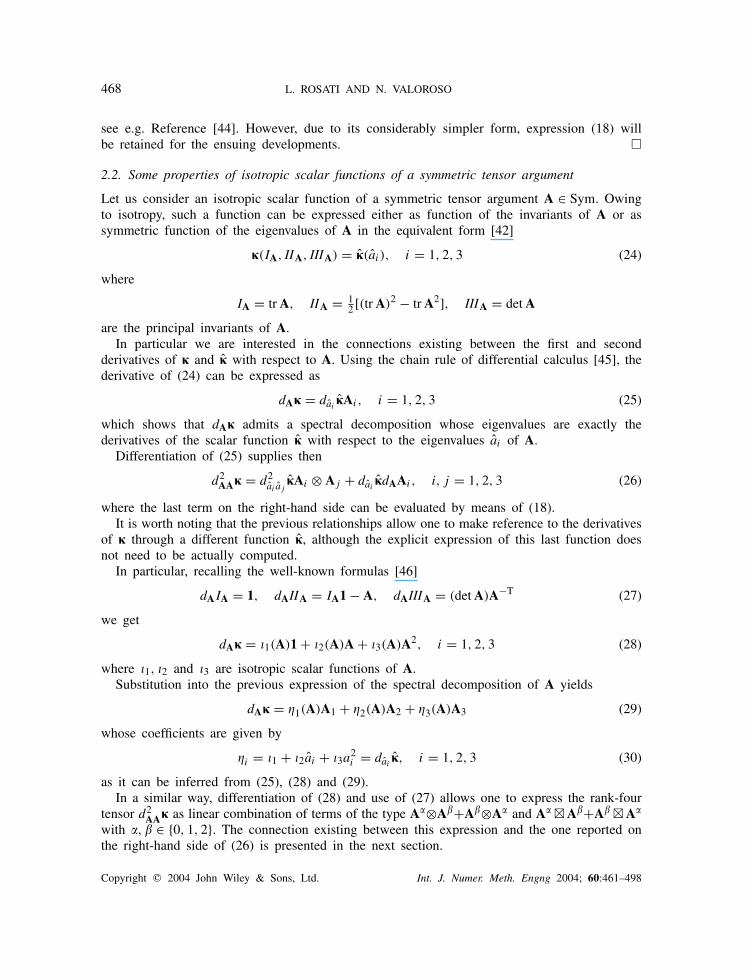
2.2. Some properties of isotropic scalar functions of a symmetric tensor argument

Let us consider an isotropic scalar function of a symmetric tensor argument A ∈ Sym. Owingto isotropy, such a function can be expressed either as function of the invariants of A or assymmetric function of the eigenvalues of A in the equivalent form [42]

�(IA, IIA, IIIA) = �(ai), i = 1, 2, 3 (24)

where

IA = trA, IIA = 12 [(trA)2 − trA2], IIIA = detA

are the principal invariants of A.In particular we are interested in the connections existing between the first and second

derivatives of � and � with respect to A. Using the chain rule of differential calculus [45], thederivative of (24) can be expressed as

dA� = dai�Ai , i = 1, 2, 3 (25)

which shows that dA� admits a spectral decomposition whose eigenvalues are exactly thederivatives of the scalar function � with respect to the eigenvalues ai of A.

Differentiation of (25) supplies then

d2AA� = d2

ai aj�Ai ⊗ Aj + dai

�dAAi , i, j = 1, 2, 3 (26)

where the last term on the right-hand side can be evaluated by means of (18).It is worth noting that the previous relationships allow one to make reference to the derivatives

of � through a different function �, although the explicit expression of this last function doesnot need to be actually computed.

In particular, recalling the well-known formulas [46]dAIA = 1, dAIIA = IA1 − A, dAIIIA = (detA)A−T (27)

we get

dA� = �1(A)1 + �2(A)A + �3(A)A2, i = 1, 2, 3 (28)

where �1, �2 and �3 are isotropic scalar functions of A.Substitution into the previous expression of the spectral decomposition of A yields

dA� = �1(A)A1 + �2(A)A2 + �3(A)A3 (29)

whose coefficients are given by

�i = �1 + �2ai + �3a2i = dai

�, i = 1, 2, 3 (30)

as it can be inferred from (25), (28) and (29).In a similar way, differentiation of (28) and use of (27) allows one to express the rank-four

tensor d2AA� as linear combination of terms of the type A�⊗A�+A�⊗A� and A� �A�+A� �A�

with �, � ∈ {0, 1, 2}. The connection existing between this expression and the one reported onthe right-hand side of (26) is presented in the next section.

Copyright � 2004 John Wiley & Sons, Ltd. Int. J. Numer. Meth. Engng 2004; 60:461–498

ISOTROPIC ELASTO/VISCO-PLASTIC MATERIALS 469

3. REPRESENTATION OF SYMMETRIC FOURTH-ORDER TENSORSIN PRINCIPAL SPACE

Let us consider a symmetric fourth-order tensor A expressed as linear combination of tensorproducts of second-order symmetric tensors in the form

A =2∑

�=0

2∑�=0

[p⊗��(A

� ⊗ A� + A� ⊗ A�) + p ��� (A� �A� + A� �A�)]

where A0 = 1 and p⊗�� and p �

�� are isotropic scalar functions.By virtue of Rivlin’s identities for tensor polynomials [47], A can be equivalently ex-

pressed as

A =2∑

�=0

2∑�=0

[q⊗��(A

� ⊗ A� + A� ⊗ A�)] +1∑

�=0

1∑�=0

[q ��� (A� �A� + A� �A�)] (31)

where q⊗�� and q �

�� depend upon p⊗�� and p �

�� and the invariants of A.We are interested to investigate on the expression of A resulting from the spectral rep-

resentation of A; in this respect it is easy to show that A is amenable to the followingrepresentation:

A =3∑

i,j=1a⊗ijAi ⊗ Aj +

3∑i,j=1i �=j

a �ij Ai �Aj = [A⊗] · [A⊗] + [A�] · [A�]

=

a⊗11 a⊗

12 a⊗13

a⊗12 a⊗

22 a⊗23

a⊗13 a⊗

23 a⊗33

·

A1 ⊗ A1 A1 ⊗ A2 A1 ⊗ A3

A2 ⊗ A1 A2 ⊗ A2 A2 ⊗ A3

A3 ⊗ A1 A3 ⊗ A2 A3 ⊗ A3

+

0 a�12 a�

31

a�12 0 a�

23

a�31 a�

23 0

·

O A1�A2 A1�A3

A2�A1 O A2�A3

A3�A1 A3�A2 O

(32)

in which the entries a⊗ij and a �

ij are polynomial expressions of the eigenvalues of A and of

the coefficients q⊗�� and q �

�� while the dots between arrays [ ] · [ ] used in the previous formulaindicate sum of the products of the elements having the same position.

As an example of the representation formula (32), we consider the rank-four identity tensor I.Recalling (4) and (10) we have

I =A1 ⊗ A1 + A2 ⊗ A2 + A3 ⊗ A3

+A1�A2 + A2�A1 + A2�A3 + A3�A2 + A3�A1 + A1�A3 (33)

Copyright � 2004 John Wiley & Sons, Ltd. Int. J. Numer. Meth. Engng 2004; 60:461–498

470 L. ROSATI AND N. VALOROSO

on account of Lemma 2. Hence,

I = [1⊗] · [A⊗] + [1�] · [A�] =

1 0 0

0 1 0

0 0 1

·

A1 ⊗ A1 A1 ⊗ A2 A1 ⊗ A3

A2 ⊗ A1 A2 ⊗ A2 A2 ⊗ A3

A3 ⊗ A1 A3 ⊗ A2 A3 ⊗ A3

+

0 1 1

1 0 1

1 1 0

·

O A1�A2 A1�A3

A2�A1 O A2�A3

A3�A1 A3�A2 O

(34)

A further example is represented by the second derivative of an isotropic scalar function� expressed in terms of principal invariants of a rank-two tensor A ∈ Sym. Recalling theconsiderations reported at the end of the previous section, the right-hand side of (26) can bewritten as

d2AA� =

d2a1a1

� d2a1a2

� d2a1a3

�

d2a1a2

� d2a2a2

� d2a2a3

�

d2a1a3

� d2a2a3

� d2a3a3

�

·

A1 ⊗ A1 A1 ⊗ A2 A1 ⊗ A3

A2 ⊗ A1 A2 ⊗ A2 A2 ⊗ A3

A3 ⊗ A1 A3 ⊗ A2 A3 ⊗ A3

+

0 d �12 � d �

13 �

d �12 � 0 d �

23 �

d �13 � d �

23 � 0

·

O A1�A2 A1�A3

A2�A1 O A2�A3

A3�A1 A3�A2 O

(35)

where

d �ij � = dai

� − daj�

ai − aj

, i = 1, 2, 3, j = 2, 3, 1

In the case of coalescent eigenvalues, the above formulas need to be modified as detailedin Reference [44].

We shall now prove the first of two basic results which play a paramount role in thedevelopments that follow.

Lemma 4Let A = [A⊗] · [A⊗] + [A�] · [A�] be a symmetric rank-four tensor. Then:

A positive-definite ⇐⇒{[A⊗] is positive definite

[A�] has positive off-diagonal entries

ProofBy definition:

A positive definite ⇔ AB · B > 0 ∀B �= 0, B ∈ Lin

Copyright � 2004 John Wiley & Sons, Ltd. Int. J. Numer. Meth. Engng 2004; 60:461–498

ISOTROPIC ELASTO/VISCO-PLASTIC MATERIALS 471

Let A be positive definite. Expressing B in the Cartesian frame represented by the eigen-vectors of A:

B =3∑

k,l=1bklak ⊗ al (36)

and observing that the following composition rules:

(Ai ⊗ Aj )(ak ⊗ al) ={Ai if j = k = l

0 otherwise

(Ai �Aj )(ak ⊗ al) ={ai ⊗ aj if i = k and j = l

0 otherwise

(37)

hold true on account of (6), one obtains

AB · B= a⊗11b

211 + a⊗

22b222 + a⊗

33b233 + 2a⊗

12b11b22 + 2a⊗23b22b33 + 2a⊗

13b33b11

+ a�12(b

212 + b221) + a�

23(b223 + b232) + a�

31(b231 + b213) > 0 ∀B �= 0

hence, setting [b] = [b11, b22, b33]T, one has finally

AB · B = [A⊗][b] · [b] +3∑

i,j=1i �=j

a �ij b2ij (38)

Since the previous inequality must hold for every B ∈ Lin, it must necessarily be

[A⊗][b] · [b] > 0,3∑

i,j=1i �=j

a �ij b2ij > 0, ∀B �= 0

By considering a tensor B whose associated matrix [B] in the principal reference frame forA is diagonal, the first relation allows one to infer that [A⊗] is positive-definite. Further, bychoosing a [B] having only one non-zero off-diagonal term, it turns out to be

a �ij > 0, i, j ∈ {1, 2, 3}, i �= j

Conversely, if [A⊗] is positive-definite and each a �ij > 0 (i �= j) one trivially infers from

(38) that A is positive-definite. The result is thus proved. �

3.1. Inversion of symmetric fourth-order tensors

Let us suppose that a positive definite tensor A is given in form (31), or equivalently in form(32), and that its inverse A−1 has to be computed.

This can be accomplished by virtue of two lemmas which, although proved in the sequel forthe case of interest of positive-definite tensors A, hold in general for any invertible fourth-ordertensor, see e.g. Reference [48].

Copyright � 2004 John Wiley & Sons, Ltd. Int. J. Numer. Meth. Engng 2004; 60:461–498

472 L. ROSATI AND N. VALOROSO

Lemma 5Given a symmetric positive-definite fourth-order tensor A in the form

A = [A⊗] · [A⊗] + [A�] · [A�]its inverse A−1 admits an analogous representation, i.e.

A−1 = [C⊗] · [A⊗] + [C� ] · [A�]where [C⊗] and [C� ] are 3 × 3 matrices.

ProofIn order to establish a representation formula for the fourth-order tensor A−1 consider thetensor equation:

AX = H (39)

in the unknown X. Clearly, X is a function of H and of the tensor A entering the definition(31) of A:

X = F(A,H) = A−1H (40)

Using the composition rules between tensor products (5), it is not difficult to prove that Fis an isotropic function of A and H simultaneously:

QF(A,H)QT = F(QAQT,QHQT) ∀Q ∈ Orth (41)

i.e. that QXQT is the solution of (39) provided that A and H are replaced by QAQT andQHQT, respectively.

To provide a concise proof of the final result we further assume H to be symmetric. Themost general proof can be obtained by following the same path of reasoning illustrated inReference [49] with reference to the simpler case of A = A� 1 + 1�A.

Owing to the symmetry of H and that of A, the solution of (39) is symmetric as well sothat, being F linear in H, the representation theorem for isotropic tensorial functions of twosymmetric tensor arguments, see e.g. Reference [47], yields

A−1 = aI + b(A�1 + 1�A) + c(A2�1 + 1�A2)

+ d(1 ⊗ 1) + e(A ⊗ 1 + 1 ⊗ A) + f (A2 ⊗ 1 + 1 ⊗ A2)

+ g(A ⊗ A) + h(A2 ⊗ A + A ⊗ A2) + i(A2 ⊗ A2)

Using the spectral decomposition (7) the principal space representation is

A−1 = [C⊗] · [A⊗] + [C� ] · [A�] (42)

and the result is demonstrated. �

We can now prove the next:

Lemma 6Given a symmetric positive-definite fourth-order tensor A in the form

A = [A⊗] · [A⊗] + [A�] · [A�]

Copyright � 2004 John Wiley & Sons, Ltd. Int. J. Numer. Meth. Engng 2004; 60:461–498

ISOTROPIC ELASTO/VISCO-PLASTIC MATERIALS 473

it turns out to be

A−1 = [A⊗]−1 · [A⊗] + [A�]−1 · [A�]where [A⊗]−1 is the inverse matrix of [A⊗] and [A�]−1 is the matrix whose components arethe reciprocals of the non-zero entries of [A�].ProofBy invoking representation (32) and the previous lemma, the matrices [C⊗] and [C� ] can bedetermined by enforcing the condition:

AA−1 = I

Recalling (34) one has

([A⊗] · [A⊗] + [A�] · [A�])([C⊗] · [A⊗] + [C� ] · [A�]) = [1⊗] · [A⊗] + [1�] · [A�]or, explicitly, by using the convention of repeated indices:

a⊗ij c⊗

klA⊗ij A⊗

kl + a⊗ij c�

kl A⊗ij A�

kl + a �ij c⊗

klA�ij A⊗

kl + a �ij c�

kl A�ij A�

kl = [1⊗] · [A⊗] + [1�] · [A�](43)

The computation of the previous expression requires the composition of dyadic and squaretensor products of the eigenprojectors of A; invoking (5) and (11), the following compositionrules can be established:

A⊗ij A⊗

kl = (Ai ⊗ Aj )(Ak ⊗ Al) ={Ai ⊗ Al if j = k

O otherwise

A⊗ij A�

kl = (Ai ⊗ Aj )(Ak �Al) ={Ai ⊗ Aj if j = k = l

O otherwise

A�ij A⊗

kl = (Ai �Aj )(Ak ⊗ Al) ={Ak ⊗ Al if i = j = k

O otherwise

A�ij A�

kl = (Ai �Aj )(Ak �Al) ={Ai �Aj if i = k and j = l

O otherwise

(44)

Hence, the left-hand side of (43) becomes

a⊗ij c⊗

j lA⊗il + a �

ij c�ij (A�

ij )i �=j = a⊗ij c⊗

j lAi ⊗ Al + a �ij c�

ij (Ai �Aj + Aj �Ai )i �=j

since the composition of dyadic and square tensor products of eigenprojectors yields non-zerotensors only when the factors of the square product do coincide, see e.g. (42)2,3, a circumstancewhich is, however, ruled out in the definition of [A�] given by (32).

The product a⊗ij c⊗

j l is the il-entry of the matrix [A⊗][C⊗] while a �ij c�

ij represents the

ij -entry of the product of the matrices [A� ] and [C� ] performed componentwise, i.e. bymultiplying the elements of the two matrices having the same position.

Copyright � 2004 John Wiley & Sons, Ltd. Int. J. Numer. Meth. Engng 2004; 60:461–498

474 L. ROSATI AND N. VALOROSO

This operation, denoted by the symbol ∗ in the sequel, is usually termed Hadamard’s productin the literature [50].

In conclusion, (43) simplifies to

[A⊗][C⊗] · [A⊗] + ([A�] ∗ [C� ]) · [A�] = [1⊗] · [A⊗] + [1�] · [A�]from which we infer

[A⊗][C⊗] = [1⊗] [A�] ∗ [C� ] = [1�]whence the result recalling the definition of [1⊗] and [1�] in formula (34). �

3.2. Composition of fourth-order tensors with second-order tensors

Additional operations which are useful in the applications are given by the composition of afourth-order tensor A with a second-order symmetric tensor B coaxial with the constituent Aof A, i.e.:

B = b1A1 + b2A2 + b3A3 = [b] · [EA] (45)

where

[b] =

b1

b2

b3

and [EA] =

A1

A2

A3

(46)

are the vectors collecting in turn the eigenvalues of B and the eigenprojectors of A.Specifically, we need to specialize operations such as AB, AB · B and AB ⊗ AB when a

principal representation of A is assigned. These results are contained in the following threelemmas.

Lemma 7Let A be a symmetric fourth-order tensor given as

A = [A⊗] · [A⊗] + [A�] · [A�]If B ∈ Sym is coaxial with A, it turns out to be

AB = a⊗ij bjAi = ([A⊗][b]) · [EA]

where [b] is the vector of the principal values bj of B.

ProofAccording to (45), we can write

AB = ([A⊗] · [A⊗] + [A�] · [A�])bkAk = a⊗ij A⊗

ij bkAk + a �ij A�

ij bkAk

Copyright � 2004 John Wiley & Sons, Ltd. Int. J. Numer. Meth. Engng 2004; 60:461–498

ISOTROPIC ELASTO/VISCO-PLASTIC MATERIALS 475

On the other hand, it turns out to be

A⊗ijAk = (Ai ⊗ Aj )Ak =

{Ai if j = k

0 otherwise

A�ij Ak = (Ai �Aj )Ak =

{Ai if i = j = k

0 otherwise

by virtue of (8), (9) and of the definitions of dyadic and square tensor products. Hence,

AB = a⊗ij bjAi = ([A⊗][b]) · [EA] (47)

since the elements of A�ij are square tensor products of eigenprojectors with different indices

(i �= j). �

The previous result allows us to establish the following:

Lemma 8Given a fourth-order tensor A in the form

A = [A⊗] · [A⊗] + [A�] · [A�]and B ∈ Sym coaxial with A, it turns out to be

AB · B= a⊗ij bj bi = ([A⊗][b]) · [b]

AB ⊗ AB= a⊗ij bj a

⊗klblAi ⊗ Ak = {([A⊗][b]) ⊗ ([A⊗][b])} · A⊗

The proof of these last two results immediately follows from (47).It is thus apparent from the previous two lemmas that only [A⊗] does play an effective role

in the composition of A with a second-order symmetric tensor B coaxial with the constituentA of A.

4. CONSTITUTIVE MODEL

We shall start our considerations with reference to the case of isotropic plasticity and visco-plasticity in the small deformation regime by summarizing the basic governing equations for thecontinuum problem and the relevant discrete formulation. The extension to the large deformationcase will be discussed later in this section.

4.1. Continuum formulation. Small deformations

Let us consider an elasto/viscoplastic structural model undergoing a quasi-static loading processwhose events are ordered by a pseudo-time scalar parameter t .

Copyright � 2004 John Wiley & Sons, Ltd. Int. J. Numer. Meth. Engng 2004; 60:461–498

476 L. ROSATI AND N. VALOROSO

Under the assumption of small transformations the kinematics of the deformation is charac-terized by the infinitesimal strain measure � and by the additive decomposition:

� = e + p (48)

having denoted by e and p the elastic and (visco)plastic shares, respectively. Addressing thepurely mechanical case, we shall make reference to a stored energy function given in fullydecoupled form as [51]

� = �el(e) + �h(�) (49)

where �el and �h are isotropic functions, both assumed to be twice differentiable with positivedefinite Hessian, and � is a strain-like scalar hardening variable.

The constitutive relations for the stress and the thermodynamic affinities are identified bymaking use of the classical thermodynamic argument [57]. Namely, from the isothermal dissi-pation inequality one has

� = de�el(e); q = d��h(�) (50)

where � is the Cauchy stress and q the stress-like internal variable accounting for the evolutionof the yield locus in the stress space. This last one is defined in terms of a general isotropicscalar function � which is assumed to be convex and smooth:

�(�, q) = �(I1, J2, J3) − q − Y0 (51)

where Y0 depends upon the initial uniaxial yield limits of the material

I1 = tr(�); J2 = 12 tr S

2; J3 = 13 tr S

3

are invariants of � and S = � − 13 tr(�)1 is the stress deviator.

The evolutionary equations for the (visco)plastic strain and the hardening variable are pro-vided by the principle of maximum plastic dissipation as

e = � − �d��(�, q); � = −�dq�(�, q) = � (52)

where

d��(�, q) = ��

�I11 + ��

�J2S + ��

�J3

(S2 − 2

3J21)

= n11 + n2S + n3S2 (53)

is the gradient of the yield function and � represents the continuum consistency parameter.In rate-independent plasticity � is characterized as a Lagrange multiplier obeying the load-

ing/unloading conditions in Kuhn–Tucker form

�(�, q) � 0, � � 0, ��(�, q) = 0 (54)

The class of viscoplasticity models based on the overstress law, originally introduced byPerzyna [52], can be incorporated within the same formalism by appealing to the regularizedversion of the maximum dissipation principle. Actually, the viscoplastic evolution equations can

Copyright � 2004 John Wiley & Sons, Ltd. Int. J. Numer. Meth. Engng 2004; 60:461–498

ISOTROPIC ELASTO/VISCO-PLASTIC MATERIALS 477

be expressed in the same way as in (52) by replacing the loading/unloading conditions (54)with the relationship [53]

� = 1

�〈�(�(�, q))〉 (55)

where � ∈ (0, +∞) represents a fluidity-like parameter, 〈 · 〉 is the ramp function, defined as〈x〉 = (x + |x|)/2, and � denotes the flow function, which has to be taken convex, C(1),monotone non-decreasing and vanishing on −

0 .The above-defined equations provide a constrained problem of evolution which, in order to

advance the solution within a typical time step [tn, tn+1], has to be transformed into a sequenceof constrained optimization problems via a suitable integration algorithm.

4.2. Discrete formulation and return map algorithm. Small deformations

As a consequence of the additive structure of the evolution problem, an update algorithm isclassically based on an elastic–plastic operator split [1]. In particular, the decomposition ofEquations (52) is as follows:

e= �; � = 0 elastic part (56)

e= −�d��(�, q); � = � plastic part (57)

Equations (56) along with the initial conditions

e(tn) = �(tn) − p(tn) = e0; �(tn) = �0 (58)

give an initial value problem amenable to exact solution

e = etr = e0 + ��; � = �tr = �0 (59)

The corresponding values of the stress-like variables

�tr = de�el(etr); q tr = d��h(�

tr) (60)

identify the trial stress state to be checked for plastic consistency.As shown in Reference [1], the algorithmic statement of the loading/unloading conditions

can be formulated exclusively in terms of the trial state. Accordingly, if �tr � 0 the trial stateequals the one at solution; otherwise, plastic consistency has to be restored by solving theplastic equations for which Equations (59) provide the initial conditions. In this last case, thetime integration of (52) by means of the fully implicit (backward Euler) scheme provides

e − etr = −�d��(�, q); � − �tr = � (61)

where � is the discrete algorithmic consistency parameter. It satisfies, for the rate-independentcase, the discrete consistency conditions in Kuhn–Tucker form

�(�, q) � 0; � � 0; ��(�, q) = 0 (62)

or the relation

�(�, q) = �−1( �

�t�)

(63)

Copyright � 2004 John Wiley & Sons, Ltd. Int. J. Numer. Meth. Engng 2004; 60:461–498

478 L. ROSATI AND N. VALOROSO

which expresses the discrete consistency for Perzyna-type viscoplasticity replacing the condition��(�, q) = 0, recovered in the limit as � → 0.

For plastic loading (�tr > 0) one has the residuals

r(k)e = e(k) − etr + �(k)d��

(k)

r(k)

� = �(k) − �tr − �(k)

r(k)

� = �(�(k), q(k)) − �−1( �

�t�(k)

)= �(k) − �(k)

(64)

whose linearization around the kth estimate of the solution yields [36]r(k)e

r(k)

�

r(k)

�

+

G(k) 0 d��(k)

0 (H (k))−1 −1

(d��(k))T −1 −d��

(k)

��(k+1)(k)

�q(k+1)(k)

��(k+1)(k)

= 0 (65)

being H(k) = d2���h(�

(k)) the tangent hardening modulus and G(k) the rank-four tensor:

G(k) = (d2ee�el(e

(k)))−1 + �(k)d2

���(k) (66)

It turns out to be positive-definite due to the positive definiteness of the elastic tangent andthe convexity of the yield function; accordingly, system (65) yields

��(k+1)(k) =

r(k)

� − (G(k))−1

r(k)e · d��

(k) + H(k)r(k)

�

(G(k))−1

d��(k) · d��

(k) + H(k) + d��(k)(67)

The above-outlined procedure describes a general iterative solution scheme for the stressupdate. The algorithm for the rate-independent case is trivially obtained by the previous oneby ruling out the viscosity-dependent term �(k).

4.3. The tensor G and its inverse

Equation (67) immediately reveals that a major computational burden in the solution of theboundary value problem in elasto(visco)plasticity is associated with the inversion of the fourth-order compliance tensor (66) since its inverse needs to be computed at each yielded Gausspoint of the structural model for every (local) constitutive iteration of each (global) equilibriumiteration.

An effective procedure for the computation of G−1 has been presented in Reference [34]by providing a representation formula for G−1 whose coefficients can be computed, basically,by solving a linear system of order three. This procedure was developed for the usual intrinsicformulation of small strain plasticity and yield functions expressed in terms of stress invariants.A different approach, based on the spectral decomposition of S:

S = s1S1 + s2S2 + s3S3 (68)

has been envisaged in Reference [35] in order to implement the representation formulafor G−1.

Copyright � 2004 John Wiley & Sons, Ltd. Int. J. Numer. Meth. Engng 2004; 60:461–498

ISOTROPIC ELASTO/VISCO-PLASTIC MATERIALS 479

In order to establish the relationship between the principal space formulation and the intrinsicone and to address indifferently yield functions expressed either in terms of stress invariantsor of principal values, the evaluation of G−1 is here carried out by making use of Lemma 6.

We start computing the explicit expression of G by considering the quadratic elastic potentialdefined as

�el(e) = 12

(K − 2

3G)

(tr e)2 + G tr(e2) (69)

where K and G denote the bulk and shear moduli, respectively; accordingly, the elastic tangentis given by

d2ee�el = 2GI +

(K − 2

3G)

(1 ⊗ 1) = d1I + d2(1 ⊗ 1) (70)

Since

S1 + S2 + S3 = 1

see (10), the elastic tangent is amenable to the following representation:

d2ee�el = [D⊗] · [S⊗] + [D�] · [S�]

=

d1 + d2 d2 d2

d2 d1 + d2 d2

d2 d2 d1 + d2

·

S1 ⊗ S1 S1 ⊗ S2 S1 ⊗ S3

S2 ⊗ S1 S2 ⊗ S2 S2 ⊗ S3

S3 ⊗ S1 S3 ⊗ S2 S3 ⊗ S3

+

0 d1 d1

d1 0 d1

d1 d1 0

·

O S1 �S2 S1 �S3

S2 �S1 O S2 �S3

S3 �S1 S3 �S2 O

on account of (32). By virtue of Lemma 6 it turns out to be

(d2ee�el)

−1 = [D⊗]−1 · [S⊗] + [D� ]−1 · [S�] = [D⊗] · [S⊗] + [D� ] · [S�]

where the entries d⊗ij of [D⊗] and d �

ij (i �= j) of [D� ] are

d⊗ii = d1 + 2d2

d1(d1 + 3d2)no sum on i

d⊗ij = − d2

d1(d1 + 3d2), i �= j

d �ij = 1

d1, i �= j

Copyright � 2004 John Wiley & Sons, Ltd. Int. J. Numer. Meth. Engng 2004; 60:461–498

480 L. ROSATI AND N. VALOROSO

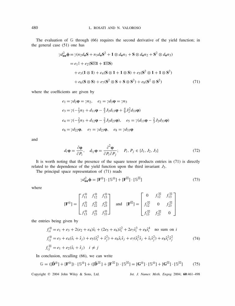
The evaluation of G through (66) requires the second derivative of the yield function; inthe general case (51) one has

�d2��� = �(n2d�S + n3d�S2 + 1 ⊗ d�n1 + S ⊗ d�n2 + S2 ⊗ d�n3)

= e1I + e2(S�1 + 1�S)

+ e3(1 ⊗ 1) + e4(S ⊗ 1 + 1 ⊗ S) + e5(S2 ⊗ 1 + 1 ⊗ S2)

+ e6(S ⊗ S) + e7(S2 ⊗ S + S ⊗ S2) + e8(S2 ⊗ S2) (71)

where the coefficients are given by

e1 = �d2� = �n2, e2 = �d3� = �n3

e3 = �(− 13n2 + d11� − 4

3J2d13� + 49J

22 d33�)

e4 = �(− 23n3 + d12� − 2

3J2d23�), e5 = �(d13� − 23J2d33�)

e6 = �d22�, e7 = �d23�, e8 = �d33�

and

di� = ��

�Pi

, dij� = �2��Pi�Pj

; Pi, Pj ∈ {I1, J2, J3} (72)

It is worth noting that the presence of the square tensor products entries in (71) is directlyrelated to the dependence of the yield function upon the third invariant J3.

The principal space representation of (71) reads

�d2��� = [F⊗] · [S⊗] + [F�] · [S�] (73)

where

[F⊗] =

f ⊗11 f ⊗

12 f ⊗13

f ⊗12 f ⊗

22 f ⊗23

f ⊗13 f ⊗

23 f ⊗33

and [F�] =

0 f �12 f �

13

f �12 0 f �

23

f �13 f �

23 0

the entries being given by

f ⊗ii = e1 + e3 + 2(e2 + e4)si + (2e5 + e6)s

2i + 2e7s

3i + e8s

4i no sum on i

f ⊗ij = e3 + e4(si + sj ) + e5(s

2i + s2j ) + e6si sj + e7(s

2i sj + si s

2j ) + e8s

2i s2j

f �ij = e1 + e2(si + sj ) i �= j

(74)

In conclusion, recalling (66), we can write

G = ([D⊗] + [F⊗]) · [S⊗] + ([D� ] + [F� ]) · [S�] = [G⊗] · [S⊗] + [G�] · [S�] (75)

Copyright � 2004 John Wiley & Sons, Ltd. Int. J. Numer. Meth. Engng 2004; 60:461–498

ISOTROPIC ELASTO/VISCO-PLASTIC MATERIALS 481

where

g⊗ii = d⊗

ii + f ⊗ii no sum

g⊗ij = d⊗

ij + f ⊗ij , i �= j

g �ij = d �

ij + f �ij , i �= j

(76)

On account of Lemma 6, the computation of the inverse of the fourth-order tensor G isequivalent to the inversion of the matrix [G⊗] collecting the coefficients of its dyadic part andto the term-by-term inversion of the matrix of the non-dyadic part [G�].

4.4. Principal space return mapping

In the algorithmic framework discussed in Section 4.2 the return mapping is entirely carriedout in intrinsic form, i.e. by making reference to tensor quantities.

As first observed in Reference [12], for the isotropic case of interest an efficient alternativeimplementation of the stress update algorithm can be obtained by using a principal axis for-mulation; moreover, Lemmas 7 and 8 show that in the computation of the return map solutiononly the dyadic part of G−1, i.e. the one pertaining to the linearization with respect to theprincipal stresses, is strictly needed. These circumstances suggest to express the return mappingalgorithm in principal space by making reference, at least formally, to a yield function givenin terms of stress eigenvalues.

Denoting by � the yield function expressed in terms of principal stresses and observing that� and etr share the same eigenvectors, we can write

(ei − etri )Si = −�d�i�Si (77)

by virtue of (25). Collecting the eigenvalues of e, etr and d�� in the vectors e, etr and d��,respectively, the return mapping can thus be reformulated as follows:

e = etr − �d�� (78)

where, according to formula (30) and (53), it turns out to be

d�i� = n1 + n2si + n3s

2i , i = 1, 2, 3

The linearization of (77) can be computed by invoking formula (35) with reference to theyield function �. In particular a comparison of formula (35) with (73) shows that

[�d2�i�j

�] = [F⊗], i, j = 1, 2, 3, �d �ij � = f �

ij , i, j = 1, 2, 3, i �= j

Note that the second term on the right-hand side of (35), stemming from the analogous onein formula (26), accounts for the change of the eigenvectors of the relevant tensor. However,this circumstance is ruled out since all tensors in the non-linear equation (78) are coaxial; thismeans that the linearization of this relationship can be carried out at constant eigenvectors, i.e.ruling out the matrix [F� ] and making reference directly to the 3× 3 positive-definite matrix:

[G(k)] = [d2ee�el(e

(k))]−1 + �(k)d2���

(k) = [G⊗](k) (79)

Copyright � 2004 John Wiley & Sons, Ltd. Int. J. Numer. Meth. Engng 2004; 60:461–498

482 L. ROSATI AND N. VALOROSO

Accordingly, setting

r(k)

e = e(k) − etr + �(k)d��(k)

(80)

one obtains the following expression for the iterative increment of the plastic parameter:

��(k+1)(k) =

r(k)

�− [G(k)]−1

r(k)

e · d��(k) + H(k)r(k)

�

[G(k)]−1d��

(k) · d��(k) + H(k) + d��(k)

(81)

and the remaining state variables can be updated according to the scheme of Table I.In summary, not only the plastic correction phase can be carried out at fixed eigenvectors

but the relevant tensorial quantities can be obtained exactly in the same way irrespective ofthe fact that the yield function is assigned in terms of invariants or of the eigenvalues of thestress tensor.

4.5. Continuum formulation. Large deformations

The phenomenological description of large-strain plasticity and viscoplasticity considered herefollows the kinematic hypothesis of Lee [54] and Mandel [55] relying upon the notion ofintermediate relaxed (stress-free) configuration.

Accordingly, we assume the multiplicative decomposition

F = FeFp (82)

where the superscripts e and p are used to denote the elastic and plastic parts of the localdeformation gradient F with Jacobian J = det F > 0.

The total, elastic and plastic strain tensors are defined in terms of the corresponding de-formation gradients; for the developments that follow we introduce the right Cauchy–Greentensors as

C = FTF; Cp = Fp,TFp (83)

which act on the reference configuration; the left Cauchy–Green tensors are defined on thecurrent (deformed) configuration and are given by

b = FFT; be = FeFe,T (84)

thus, be is the push-forward [56] of the inverse of the plastic right Cauchy–Green tensor tothe current configuration:

be = (F�F)(Cp)−1 (85)

As in the linearized theory, we shall assume that the elastic behaviour is unaffected by thespread of inelastic deformation; accordingly, given the functional restrictions imposed by theprinciple of frame invariance [46] and on account of elastic isotropy, the free energy potentialin the spatial description is taken as

� = �el(be) + �h(�) = �el(Ii(be)) + �h(�) (86)

where Ii(be), i ∈ {1, 2, 3}, are the principal invariants of be.

Copyright � 2004 John Wiley & Sons, Ltd. Int. J. Numer. Meth. Engng 2004; 60:461–498

ISOTROPIC ELASTO/VISCO-PLASTIC MATERIALS 483

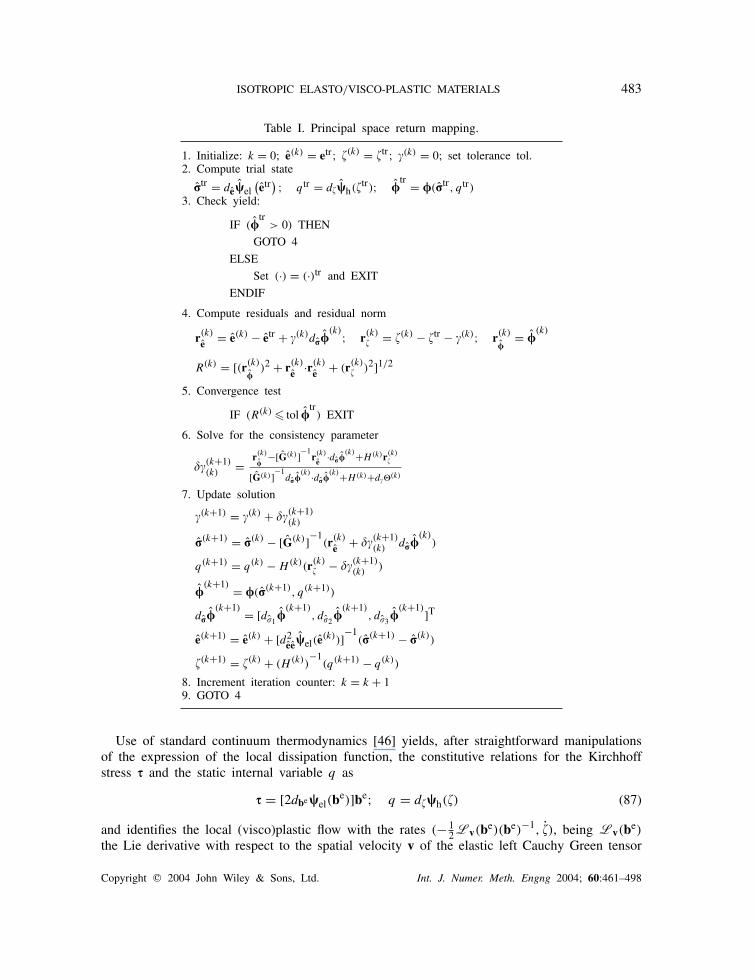
Table I. Principal space return mapping.

1. Initialize: k = 0; e(k) = etr ; �(k) = �tr ; �(k) = 0; set tolerance tol.2. Compute trial state

�tr = de�el(etr

) ; qtr = d��h(�tr); �

tr = �(�tr, qtr)3. Check yield:

IF (�tr

> 0) THEN

GOTO 4

ELSE

Set (·) = (·)tr and EXIT

ENDIF

4. Compute residuals and residual norm

r(k)

e = e(k) − etr + �(k)d��(k); r(k)

� = �(k) − �tr − �(k); r(k)

�= �

(k)

R(k) = [(r(k)

�)2 + r(k)

e ·r(k)

e + (r(k)� )2]1/2

5. Convergence test

IF (R(k) � tol �tr) EXIT

6. Solve for the consistency parameter

��(k+1)(k)

= r(k)

�−[G(k)]−1

r(k)

e ·d��(k)+H(k)r(k)

�

[G(k)]−1d��

(k)·d��(k)+H(k)+d��(k)

7. Update solution

�(k+1) = �(k) + ��(k+1)(k)

�(k+1) = �(k) − [G(k)]−1(r(k)

e + ��(k+1)(k)

d��(k)

)

q(k+1) = q(k) − H(k)(r(k)� − ��(k+1)

(k))

�(k+1) = �(�(k+1)

, q(k+1))

d��(k+1) = [d�1

�(k+1)

, d�2�

(k+1), d�3

�(k+1)]T

e(k+1) = e(k) + [d2ee�el(e(k))]−1

(�(k+1) − �(k))

�(k+1) = �(k) + (H(k))−1

(q(k+1) − q(k))

8. Increment iteration counter: k = k + 19. GOTO 4

Use of standard continuum thermodynamics [46] yields, after straightforward manipulationsof the expression of the local dissipation function, the constitutive relations for the Kirchhoffstress � and the static internal variable q as

� = [2dbe�el(be)]be; q = d��h(�) (87)

and identifies the local (visco)plastic flow with the rates (− 12Lv(be)(be)−1, �), being Lv(be)

the Lie derivative with respect to the spatial velocity v of the elastic left Cauchy Green tensor

Copyright � 2004 John Wiley & Sons, Ltd. Int. J. Numer. Meth. Engng 2004; 60:461–498

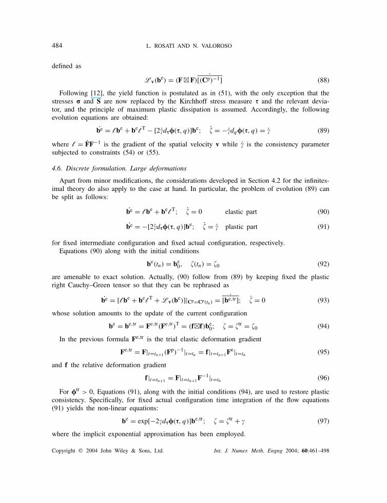
484 L. ROSATI AND N. VALOROSO

defined as

Lv(be) = (F�F)˙[(Cp)−1] (88)

Following [12], the yield function is postulated as in (51), with the only exception that thestresses � and S are now replaced by the Kirchhoff stress measure � and the relevant devia-tor, and the principle of maximum plastic dissipation is assumed. Accordingly, the followingevolution equations are obtained:

be = lbe + belT − [2�d��(�, q)]be; � = −�dq�(�, q) = � (89)

where l = FF−1 is the gradient of the spatial velocity v while � is the consistency parametersubjected to constraints (54) or (55).

4.6. Discrete formulation. Large deformations

Apart from minor modifications, the considerations developed in Section 4.2 for the infinites-imal theory do also apply to the case at hand. In particular, the problem of evolution (89) canbe split as follows:

be = lbe + belT; � = 0 elastic part (90)

be = −[2�d��(�, q)]be; � = � plastic part (91)

for fixed intermediate configuration and fixed actual configuration, respectively.Equations (90) along with the initial conditions

be(tn) = be0, �(tn) = �0 (92)

are amenable to exact solution. Actually, (90) follow from (89) by keeping fixed the plasticright Cauchy–Green tensor so that they can be rephrased as

be = [lbe + belT + Lv(be)]|Cp=Cp(tn) = ˙[be,tr]; � = 0 (93)

whose solution amounts to the update of the current configuration

be = be,tr = Fe,tr(Fe,tr)T = (f�f)be0; � = �tr = �0 (94)

In the previous formula Fe,tr is the trial elastic deformation gradient

Fe,tr = F|t=tn+1(Fp)−1|t=tn = f |t=tn+1F

e|t=tn (95)

and f the relative deformation gradient

f |t=tn+1 = F|t=tn+1F−1|t=tn (96)

For �tr > 0, Equations (91), along with the initial conditions (94), are used to restore plasticconsistency. Specifically, for fixed actual configuration time integration of the flow equations(91) yields the non-linear equations:

be = exp[−2�d��(�, q)]be,tr; � = �tr + � (97)

where the implicit exponential approximation has been employed.

Copyright � 2004 John Wiley & Sons, Ltd. Int. J. Numer. Meth. Engng 2004; 60:461–498

ISOTROPIC ELASTO/VISCO-PLASTIC MATERIALS 485

The use of the exponential map for the time integration of (89)1, as originally proposedin Reference [57], is well known to entail some important algorithmic properties namely, thepreservation of the plastic volume for pressure-insensitive yield criteria and a particularly simpleform of the return mapping algorithm in principal space [12]. This last property stems fromthe fact that, under the assumption of isotropy, all terms in (97)1 commute so that the returnmapping takes place at fixed eigenvectors which are obtained from the symmetric eigenvalueproblem:

[be,tr − (e,tri )21]stri = 0 (98)

where e,tri are the principal elastic trial stretches and stri the relevant eigenvectors.Hence, by expressing (97)1 with reference to principal axes and taking the logarithm of

both sides one obtains the same equation as in (78) with e and etr being now replaced by thevectors of principal values of the elastic logarithmic strain tensors:

e = 12 ln(b

e); etr = 12 ln(b

e,tr) (99)

With this result at hand, and noting that the isotropy assumption for the elastic potentialentails a constitutive relation for the principal values of the Kirchhoff stress completely similarto the one holding in the infinitesimal case, i.e.: � = de�el(e), it is immediate to recognizethat the principal return mapping does possess the same structure of that of the infinitesimaltheory. In particular, taking the Hencky potential:

�el(e) = 1

2

(K − 2

3G

)(ln J e)2 + G

3∑i=1

(ln ei )2 (100)

where J e = det (Fe) is the elastic Jacobian and K and G are the usual elastic moduli, thespectral return mapping algorithm discussed in Section 4.4 applies with no modification.

4.7. Consistent tangent operator

An essential ingredient for the efficient solution of the discretized boundary value problemarising in elasto(visco)plasticity via Newton’s method is the computation of the consistenttangent tensor [4]. In particular, the objective of this section is that of evaluating the constitutiveor material tangent; as opposite to the local algorithm linearization, in which no change in theprincipal vectors is accounted for, the material contribution to the tangent tensor requires thefull linearization of the discretized constitutive relations.

We shall first examine the large deformation case for which, in the adopted formulation, thedevised relation is [8]

�◦ = Etand (101)

where �◦ is the Truesdell rate [56] of the Cauchy stress, d is the rate of deformation tensorand Etan is the material contribution to the spatial elasto(visco)plastic tangent.

In order to work out the expression of Etan we start by computing the tangent moduli tensorrelative to the intermediate relaxed configuration, which is in turn obtained as the gradient of

Copyright � 2004 John Wiley & Sons, Ltd. Int. J. Numer. Meth. Engng 2004; 60:461–498

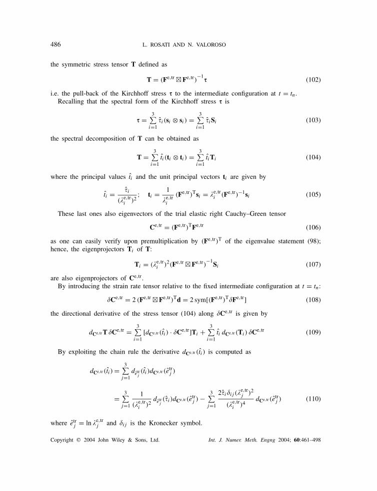
486 L. ROSATI AND N. VALOROSO

the symmetric stress tensor T defined as

T = (Fe,tr �Fe,tr)−1

� (102)

i.e. the pull-back of the Kirchhoff stress � to the intermediate configuration at t = tn.Recalling that the spectral form of the Kirchhoff stress � is

� =3∑

i=1i (si ⊗ si ) =

3∑i=1

iSi (103)

the spectral decomposition of T can be obtained as

T =3∑

i=1ti (ti ⊗ ti ) =

3∑i=1

tiTi (104)

where the principal values ti and the unit principal vectors ti are given by

ti = i

(e,tri )2; ti = 1

e,tri

(Fe,tr)Tsi = e,tri (Fe,tr)−1si (105)

These last ones also eigenvectors of the trial elastic right Cauchy–Green tensor

Ce,tr = (Fe,tr)TFe,tr (106)

as one can easily verify upon premultiplication by (Fe,tr)T of the eigenvalue statement (98);hence, the eigenprojectors Ti of T:

Ti = (e,tri )2(Fe,tr �Fe,tr)−1

Si (107)

are also eigenprojectors of Ce,tr .By introducing the strain rate tensor relative to the fixed intermediate configuration at t = tn:

�Ce,tr = 2 (Fe,tr �Fe,tr)Td = 2 sym[(Fe,tr)T�Fe,tr] (108)

the directional derivative of the stress tensor (104) along �Ce,tr is given by

dCe,trT �Ce,tr =3∑

i=1[dCe,tr (ti ) · �Ce,tr]Ti +

3∑i=1

ti dCe,tr (Ti ) �Ce,tr (109)

By exploiting the chain rule the derivative dCe,tr (ti ) is computed as

dCe,tr (ti ) =3∑

j=1detrj

(ti )dCe,tr (etrj )

=3∑

j=1

1

(e,tri )2detrj

(i )dCe,tr (etrj ) −3∑

j=1

2i�ij (e,trj )2

(e,tri )4dCe,tr (etrj ) (110)

where etrj = ln e,trj and �ij is the Kronecker symbol.

Copyright � 2004 John Wiley & Sons, Ltd. Int. J. Numer. Meth. Engng 2004; 60:461–498

ISOTROPIC ELASTO/VISCO-PLASTIC MATERIALS 487

Since (e,trj )2 are eigenvalues of Ce,tr , Lemma 1 supplies

dCe,tr ((e,trj )2) = Tj (111)

from which we infer

dCe,tr (etrj ) = 1

2(e,trj )2Tj (112)

Accordingly, the first term on the right-hand side of (109) is

3∑i=1

[dCe,tr (ti ) · �Ce,tr]Ti =3∑

i,j=1

1

2(e,tri )2(e,trj )2detrj

(i )(Ti ⊗ Tj )�Ce,tr

−3∑

i=1

i

(e,tri )4(Ti ⊗ Ti )�Ce,tr (113)

Further, invoking relation (18) one has

dCe,tr Ti = Ti �Tj + Tj �Ti

(e,tri )2 − (e,trj )2+ Ti �Tk + Tk �Ti

(e,tri )2 − (e,trk )2, i �= j, k (114)

so that the second term on the right-hand side of (109) becomes

3∑i=1

ti dCe,tr (Ti ) �Ce,tr =3∑

i,j=1i �=j

ti − tj

(e,tri )2 − (e,trj )2(Ti �Tj )�Ce,tr

=3∑

i,j=1i �=j

1

(e,tri )2(e,trj )2

i (e,trj )2 − j (

e,tri )2

(e,tri )2 − (e,trj )2(Ti �Tj )�Ce,tr (115)

The spatial tangent defined by (101) can now be given an explicit expression by exploitingthe push-forward relations [56]:

�◦ = 1

JLv(�) = 1

J(Fe,tr �Fe,tr)dCe,trT�Ce,tr (116)

2d=Lv(1) = (Fe,tr �Fe,tr)−T�Ce,tr (117)

Accordingly, use of (116) and (117) yields

Etan = 1

J

3∑i,j=1

detrj(i )(Si ⊗ Sj ) −

3∑i=1

2�i (Si ⊗ Si ) +3∑

i,j=1i �=j

2�i (

e,trj )2 − �j (

e,tri )2

(e,tri )2 − (e,trj )2(Si �Sj )

(118)

Copyright � 2004 John Wiley & Sons, Ltd. Int. J. Numer. Meth. Engng 2004; 60:461–498

488 L. ROSATI AND N. VALOROSO

By virtue of (6)1 the previous expression coincides with formula (A.33) reported in Reference[8]. It is then immediate to verify that such formulas have the same structure as for theLagrangian description of multiplicative elastoplasticity; see e.g. Equations (34)–(35) and (46)of Reference [8].

To obtain the final expression of the spatial tangent it remains to evaluate the term

3∑i,j=1

detrj(i )(Si ⊗ Sj ) = [detr �] · [S⊗]

i.e. the dyadic part of the derivative detr�.This term can be computed from the linearization of the principal return mapping algorithm

at the local converged state (t = tn+1) by considering the system

−�etr

0

0

+

[G⊗] 0 d��

0 [H ]−1 −1

(d��)T −1 −d��

detr �

detrq

detr�

= 0 (119)

whose solution with respect to detr � yields

detr � = [G⊗]−1 − [G⊗]−1d�� ⊗ [G⊗]−1d��

[G⊗]−1d�� · d�� + H + d��(120)

that exactly coincides with the dyadic part of the consistent tangent of the infinitesimal theory,see e.g. Reference [35].

With reference to this last case, by following a path of reasoning identical to the oneexploited before, one can compute the derivative of the Cauchy stress with respect to theinfinitesimal trial elastic strain etr as

detr� =3∑

i,j=1detrj

(�i )(Si ⊗ Sj ) +3∑

i,j=1i �=j

�i − �j

etri − etrj(Si �Sj ) (121)

in which the coefficients multiplying the terms Si �Sj can be easily shown to coincide withthe reciprocals of the terms g �

ij defined in (76). In this respect, by observing that

�i − �j

etri − etrj= 2G

si − sj

stri − strj(122)

where stri is the ith principal value of the deviator of the trial Cauchy stress, it is immediateto verify that the return map solution for si − sj is given by

si − sj = stri − strj − 2G�(si − sj )[n2 + n3(si + sj )] (123)

with n2, n3 given as in (53); accordingly

si − sj

stri − strj= 1

1 + 2G�[n2 + n3(si + sj )] = 1

2G

1

g �ij

(124)

Copyright � 2004 John Wiley & Sons, Ltd. Int. J. Numer. Meth. Engng 2004; 60:461–498

ISOTROPIC ELASTO/VISCO-PLASTIC MATERIALS 489

As clearly shown by the previous formulas, the square tensor product terms in the expressionof the tangent tensor are due to the change in the eigenvectors; in the small deformation case thisis simply accounted for by the non-dyadic part of the tensor G while in the finite deformationcase the non-dyadic part of the tangent tensor, which originates from the push-forward of (115),is slightly more complicated due to the non-linearity of the strain measure.

As a final remark, we emphasize that the above expressions provide the consistent tangentoperator directly in the given reference frame. Indeed, the spectral representation of the stresstensor implies that the matrix [Si] = [si ⊗ si] of the generic eigenprojector is assigned in thesame reference frame as that of [S] so that no co-ordinate transformation between the principalframe and the reference Cartesian one is needed for implementing the consistent tangent.

5. NUMERICAL EXAMPLE

To demonstrate the performance of the solution scheme discussed in the previous sections anumerical example is presented. The simulation refers to an isotropic model defined throughthe following pressure-insensitive yield function:

�(J2, J3) = [2J2]1/2r(�)

− f ′c (125)

where f ′c is the magnitude of the limit stress in uniaxial compression and r(�) is a function

defining the shape of the failure surface in the deviatoric plane:

r(�) = rc2(r2c − r2t ) cos � − (rc − 2rt)[4(r2c − r2t ) cos2 � + 5r2t − 4rcrt]1/2

4(r2c − r2t ) cos2 � + (rc − 2rt)2(126)

The parameter � is the Lode angle defined as

� = 1

3arccos

3√3

2

J3

J3/22

, � ∈[0,

�

3

](127)

where the constants rt and rc are non-dimensional material parameters of the model whichare representative of the shear strength on the tensile and compressive meridians; they arecomputed from the uniaxial tensile and compressive limits as rt = √

2/3f ′t /f

′c and rc = √

2/3.The deviatoric section of the yield locus defined by (125) is plotted in Figure 1.

Equation (126) has been originally proposed by Willam and Warnke in Reference [21] as apart of the celebrated five parameter model, which is one of the most successful descriptionsof the triaxial failure envelope of concrete; moreover, the same expression has been used formodelling soil behaviour [58]. This equation defines a smooth elliptic interpolation betweenthe tensile (� = 0) and compressive (� = �/3) meridians which results in a surface possessingconvexity within the range 1

2 � rt/rc � 1. For a detailed account on the derivation of (126) thereader may refer to Reference [22].

For rt/rc = 1 the influence of the J3 invariant through the Lode angle � is dropped outand the yield surface collapses to the Von Mises cylinder, while the minimum shape factor

Copyright � 2004 John Wiley & Sons, Ltd. Int. J. Numer. Meth. Engng 2004; 60:461–498

490 L. ROSATI AND N. VALOROSO

Figure 1. Deviatoric sections of the yield locus.

rt/rc = 12 corresponds to a triangular shape of the deviatoric section described by

�(J2, J3) = [2J2]1/22 cos � −[2

3

]1/2f ′c (128)

5.1. Elastic–plastic plate with flat hole

The numerical example here considered has been first analysed in Reference [59] to test thebehaviour of stabilized mixed finite element methods in the framework of finite elasticity.The problem consists of the large-strain analysis of a square plate with a central slot underplane strain which is subject to normal boundary conditions along the whole outer edge andto imposed displacements � in the vertical direction; see Figure 2. For the finite elementanalysis only a quarter of the plate has been modelled with 366 Q1/P0 plane elements byapplying the appropriate symmetry boundary conditions. The loading history is of cyclic type,see Figure 3, and has been assigned using three different sets of initial time increments:�t = 0.4, 0.5, 1.0. Elastic-perfectly plastic behaviour has been considered; the elastic propertiesare taken as K = 8333.3 and G = 3846.15 and the data set for the yield limits are:

(i) f ′t = f ′

c = 100.0;(ii) f ′

t = 100.0; f ′c = 142.86;

(iii) f ′t = 100.0; f ′

c = 185.71;

which correspond to a shape factor rc/rt for the yield surface equal to 1, 10/7, 13/7, re-spectively; see also Figure 1. The relevant load–deflection curves are reported in Figure 4

Copyright � 2004 John Wiley & Sons, Ltd. Int. J. Numer. Meth. Engng 2004; 60:461–498

ISOTROPIC ELASTO/VISCO-PLASTIC MATERIALS 491

Figure 2. Square strip with a slot. Model problem and finite elements mesh.

Figure 3. Plate with flat hole. Loading data.

and refer to the solution obtained for �t = 0.4. Computations have been carried out byusing a customized version of the finite element code FEAP rel. 7.1b [60]; all of themhave been successfully completed in 125, 100 and 50 load steps by using a local linear linesearch scheme to render the return map algorithm globally convergent. In the numerical ex-

Copyright � 2004 John Wiley & Sons, Ltd. Int. J. Numer. Meth. Engng 2004; 60:461–498

492 L. ROSATI AND N. VALOROSO

Figure 4. Plate with flat hole. Load–deflection curves. �t = 0.4.

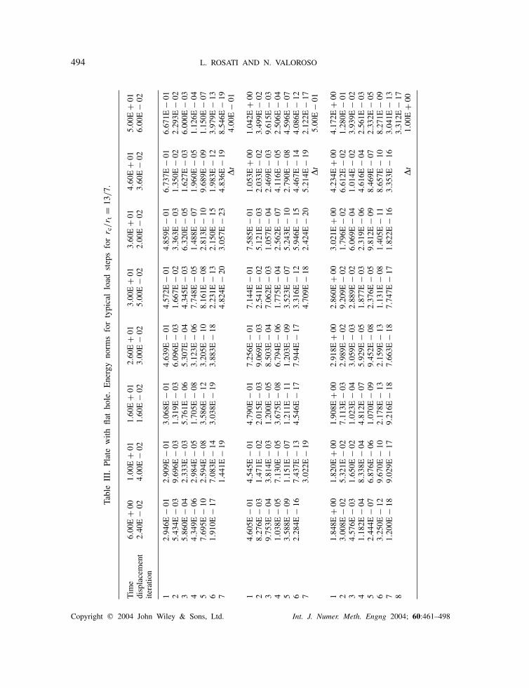
amples described below use has been made of a global termination criterion expressed interms of the incremental energy norm [11] with a tolerance = 10−16. The convergencebehaviour is illustrated in Tables II and III in terms of this norm for some typical loadsteps.

6. CONCLUDING REMARKS

A unified approach for the formulation and implementation of isotropic elasto(visco)plasticmodels endowed with yield functions of arbitrary type has been presented. The algorithmicframework detailed in the paper is exactly the same irrespective of the fact that the yieldfunction is assigned in terms of the set of stress invariants (I1, J2, J3) or of stress eigenvalues.The result has been achieved by exploiting some original results, proved in the paper, concerningrank-four tensors A obtained as second derivatives of isotropic scalar functions of a symmetricrank-two tensor A and the differentiation of the eigenprojectors Ak of A with respect to thetensor A.

In particular, the derivative of the eigenprojectors of rank-two symmetric tensors with respectto the tensor itself has been provided by an original formula, more compact than the existingones. The contributed expression clarifies the meaning and the role of the square tensor productsentering the expression of the material tangent tensor which is used in the solution of theelasto(visco)plastic boundary value problem via Newton’s method.

In the detailed framework the state variables and the tangent tensor are always referred tothe global co-ordinate system so that no co-ordinate transformation is needed for the numericalimplementation.

The specialization of the proposed approach to the significant class of plane stress problemswill be pursued in a forthcoming paper.

Copyright � 2004 John Wiley & Sons, Ltd. Int. J. Numer. Meth. Engng 2004; 60:461–498

ISOTROPIC ELASTO/VISCO-PLASTIC MATERIALS 493

TableII.Platewith

flathole.Energynorm

sfortypicalload

stepsfor

r c/r t

=10

/7.

Tim

e6.00

E+

001.00

E+

011.60

E+

012.60

E+

013.00

E+

013.60

E+

014.60

E+

015.00

E+

01displacement

2.40

E−

024.00

E−

021.60

E−

023.00

E−

025.00

E−

022.00

E−

023.60

E−

026.00

E−

02ite

ratio

n

12.95

4E−

012.94

0E−

013.09

6E−

014.67

8E−

014.64

8E−

014.91

4E−

016.82

9E−

016.79

3E−

012

8.27

1E−

031.66

0E−

022.17

6E−

031.17

8E−

022.59

9E−

025.58

0E−

031.68

9E−

023.23

0E−

023

4.94

8E−

041.11

9E−

031.81

3E−

058.70

0E−

042.16

5E−

039.56

9E−

051.49

5E−

033.98

1E−

034

6.83

1E−

061.46

9E−

051.27

7E−

084.21

4E−

064.15

4E−

052.01

6E−

071.02

5E−

051.56

8E−

045

2.49

7E−

095.96

8E−

093.53

3E−

147.04

0E−

103.52

0E−

084.05

5E−

123.88

0E−

098.41

3E−

076

1.77

2E−

151.90

0E−

151.55

5E−

244.68

0E−

173.95

7E−

142.22

4E−

203.05

7E−

152.48

6E−

127

5.98

1E−

271.55

9E−

255.35

9E−

242.96

0E−

267.41

6E−

22�

t4.00

E−

01

14.61

8E−

014.59

4E−

014.83

4E−

017.31

5E−

017.26

2E−

017.67

4E−

011.06

8E+

001.06

1E+

002

1.23

8E−

022.48

4E−

023.30

8E−

031.69

9E−

023.88

9E−

028.45

4E−

032.54

0E−

024.80

3E−

023

9.61

3E−

042.18

8E−

033.42

7E−

051.41

0E−

034.11

9E−

031.87

6E−

042.52

6E−

037.01

6E−

034

1.94

4E−

054.40

3E−

053.72

8E−

081.12

9E−

051.15

9E−

045.29

9E−

072.59

7E−

053.92

3E−

045

1.62

9E−

084.31

9E−

082.59

6E−

133.75

5E−

092.25

4E−

071.91

3E−

111.68

1E−

085.75

0E−

066

2.17

6E−

144.20

4E−

138.13

3E−

231.08

1E−

171.32

2E−

124.49

7E−

192.05

2E−

142.17

8E−

097

3.66

1E−

236.52

4E−

234.57

7E−

223.64

8E−

258.68

2E−

18�

t5.00

E−

01

11.85

2E+

001.83

8E+

001.92

7E+

002.93

9E+

002.90

4E+

003.06

0E+

004.28

7E+

004.24

5E+

002

4.23

8E−

028.27

9E−

021.17

6E−

025.16

7E−

021.29

8E−

012.95

6E−

029.15

2E−

021.58

8E−

013

6.55

3E−

031.46

3E−

022.77

4E−

048.87

8E−

032.31

9E−

021.51

0E−

032.11

4E−

023.53

3E−

024

3.21

1E−

048.72

5E−

041.90

7E−

061.88

9E−

041.77

3E−

031.05

0E−

054.97

1E−

043.79

4E−

035

2.17

9E−

068.47

8E−

062.53

0E−

082.89

1E−

072.91

8E−

055.85

9E−

091.67

9E−

069.69

1E−

056

2.05

7E−

102.00

5E−

091.57

3E−

111.54

8E−

121.61

5E−

082.35

8E−

145.61

3E−

101.44

5E−

077

7.04

6E−

173.95

8E−

147.09

6E−

188.89

6E−

213.82

8E−

136.51

8E−

211.95

2E−

131.04

5E−

128

4.00

8E−

219.12

3E−

221.22

2E−

202.36

1E−

18�

t1.00

E+

00

Copyright � 2004 John Wiley & Sons, Ltd. Int. J. Numer. Meth. Engng 2004; 60:461–498

494 L. ROSATI AND N. VALOROSO

TableIII.

Platewith

flathole.Energynorm

sfortypicalload

stepsfor

r c/r t

=13

/7.

Tim

e6.00

E+

001.00

E+

011.60

E+

012.60

E+

013.00

E+

013.60

E+

014.60

E+

015.00

E+

01displacement

2.40

E−

024.00

E−

021.60

E−

023.00

E−

025.00

E−

022.00

E−

023.60

E−

026.00

E−

02ite

ratio

n

12.94

6E−

012.90

9E−

013.06

8E−

014.63

9E−

014.57

2E−

014.85

9E−

016.73

7E−

016.67

1E−

012

5.43

4E−

039.69

6E−

031.31

9E−

036.09

6E−

031.66

7E−

023.36

3E−

031.35

0E−

022.29

3E−

023

5.86

0E−

042.33

3E−

035.76

1E−

065.30

7E−

044.34

5E−

036.32

0E−

051.62

7E−

036.00

0E−

034

4.34

9E−

062.98

4E−

051.70

5E−

083.12

3E−

067.74

8E−

051.48

8E−

071.96

0E−

051.12

6E−

045

7.69

5E−

102.59

4E−

083.58

6E−

123.20

5E−

108.16

1E−

082.81

3E−

109.68

9E−

091.15

0E−

076

1.91

0E−

177.08

3E−

143.03

8E−

193.88

3E−

182.23

1E−

132.15

0E−

151.98

3E−

123.97

9E−

137

1.44

1E−

194.82

4E−

203.05

7E−

234.83

6E−

198.54

6E−

19�

t4.00

E−

01

14.60

5E−

014.54

5E−

014.79

0E−

017.25

6E−

017.14

4E−

017.58

5E−

011.05

3E+

001.04

2E+

002

8.27

6E−

031.47

1E−

022.01

5E−

039.06

9E−

032.54

1E−

025.12

1E−

032.03

3E−

023.49

9E−

023

9.75

3E−

043.81

4E−

031.20

0E−

058.50

3E−

047.06

2E−

031.05

7E−

042.46

9E−

039.61

5E−

034

1.03

8E−

057.13

0E−

053.67

5E−

086.79

4E−

061.77

5E−

042.56

2E−

074.11

6E−

052.50

6E−

045

3.58

8E−

091.15

1E−

071.21

1E−

111.20

3E−

093.52

3E−

075.24

3E−

102.79

0E−

084.59

6E−

076

2.28

4E−

167.43

7E−

134.54

6E−

177.94

4E−

173.31

6E−

125.94

6E−

154.46

7E−

144.08

6E−

127

3.02

2E−

194.70

9E−

182.42

4E−

205.21

4E−

192.12

2E−

17�

t5.00

E−

01

11.84

8E+

001.82

0E+

001.90

8E+

002.91

8E+

002.86

0E+

003.02

1E+

004.23

4E+

004.17

2E+

002

3.00

8E−

025.32

1E−

027.11

3E−

032.98

9E−

029.20

9E−

021.79

6E−

026.61

2E−

021.28

0E−

013

4.57

6E−

031.65

0E−

021.02

3E−

043.05

9E−

032.88

9E−

026.06

9E−

041.01

4E−

023.93

9E−

024

1.18

2E−

048.33

8E−

044.81

2E−

075.92

9E−

051.87

7E−

032.31

9E−

064.61

6E−

042.56

1E−

035

2.44

4E−

076.87

6E−

061.07

0E−

099.45

2E−

082.37

6E−

059.81

2E−

098.46

9E−

072.33

2E−

056

3.25

0E−

129.67

0E−

102.17

8E−

132.15

9E−

131.13

1E−

081.40

5E−

118.65

7E−

108.27

1E−

097

1.20

0E−

189.02

9E−

179.21

6E−

187.66

3E−

187.74

7E−

171.82

2E−

163.35

3E−

163.04

1E−

138

3.31

2E−

17�

t1.00

E+

00

Copyright � 2004 John Wiley & Sons, Ltd. Int. J. Numer. Meth. Engng 2004; 60:461–498

ISOTROPIC ELASTO/VISCO-PLASTIC MATERIALS 495

APPENDIX A

For the sake of completeness, we provide hereafter the matrix representations of the fourth-order tensors referred to in the body of the paper. Additional details on this topic can be foundin Reference [61].

The Cartesian components of the dyadic and the square tensor products between rank-twotensors A, B ∈ Lin are

(A ⊗ B)ijkl = AijBkl (A�B)ijkl = AikBj l ∀A, B ∈ Lin

Consistent with the tensor-to-matrix mapping commonly employed in the computational me-chanics literature [9, 11], stress-(T) and strain-like (D) rank-two symmetric tensors are expressedin vector form as follows:

T= [T11, T22, T33, T12, T23, T31]D= [D11, D22, D33, 2D12, 2D23, 2D31]

Accordingly, given A,B ∈ Sym, a fourth-order tensor A⊗B mapping strain to stress tensorsis amenable to the following matrix representation:

[A ⊗ B] =

A11B11 A11B22 A11B33 A11B12 A11B23 A11B31

A22B11 A22B22 A22B33 A22B12 A22B23 A22B31

A33B11 A33B22 A33B33 A33B12 A33B23 A33B31

A12B11 A12B22 A12B33 A12B12 A12B23 A12B31

A23B11 A23B22 A23B33 A23B12 A23B23 A23B31

A31B11 A31B22 A31B33 A31B12 A31B23 A31B31

which trivially follows from the definition of the dyadic tensor product. Analogously, from thedefinition of the square tensor product, it is not difficult to show that

[A�B] =

A11B11 A12B12 A13B13A11B12 + A12B11

2

A12B13 + A13B12

2

A13B11 + A11B13

2

A21B21 A22B22 A23B23A21B22 + A22B21

2

A22B23 + A23B22

2

A23B21 + A21B23

2

A31B31 A32B32 A33B33A31B32 + A32B31

2

A32B33 + A33B32

2

A33B31 + A31B33

2

A11B21 A12B22 A13B23A11B22 + A12B21

2

A12B23 + A13B22

2

A13B21 + A11B23

2

A21B31 A22B32 A23B33A21B32 + A22B31

2

A22B33 + A23B32

2

A23B31 + A21B33

2

A31B11 A32B12 A33B13A31B12 + A32B11

2

A32B13 + A33B12

2

A33B11 + A31B13

2

and I = 1 × 1 = diag[1, 1, 1, 1/2, 1/2, 1/2].

Copyright � 2004 John Wiley & Sons, Ltd. Int. J. Numer. Meth. Engng 2004; 60:461–498

496 L. ROSATI AND N. VALOROSO

ACKNOWLEDGEMENTS

The authors acknowledge the Italian National Research Council (CNR) and the Italian Ministry ofEducation, University and Research (MIUR) for the financial support.

This work has been partly carried out within the framework of the activities of the LaboratoireLagrange, a European research group gathering CNR, CNRS, Università di Roma ‘Tor Vergata,’Université de Montpellier II, ENPC, LCPC.

REFERENCES

1. Simo JC, Hughes TJR. Computational Inelasticity. Springer: New York, 1998.2. Simo JC. Numerical analysis and simulation of plasticity. In Handbook of Numerical Analysis, Ciarlet PG,

Lyons J-L (eds), vol. VI. Elsevier: Amsterdam, 1998.3. Hofstetter G, Simo JC, Taylor RL. A modified cap model: closest point solution algorithms. Computers and

Structures 1993; 46:203–214.4. Simo JC, Taylor RL. Consistent tangent operators for rate-independent elastoplasticity. Computer Methods in

Applied Mechanics and Engineering 1985; 48:101–118.5. Simo JC, Taylor RL, Pister KS. Variational and projection methods for the volume constraint in finite

deformation elasto-plasticity. Computer Methods in Applied Mechanics and Engineering 1985; 51:177–208.6. Simo JC, Taylor RL. A return mapping algorithm for plane stress elastoplasticity. International Journal for

Numerical Methods in Engineering 1986; 22:649–670.7. Simo JC, Ju W, Pister KS, Taylor RL. An assessment of the cap model: consistent return algorithms and

rate-dependent extensions. Journal of Engineering Mechanics (ASME) 1988; 144:191–218.8. Bonet J, Wood RD. Nonlinear Continuum Mechanics for Finite Element Analysis. Cambridge University

Press: Cambridge, MA, 1997.9. Crisfield MA. Non-linear Finite Element Analysis of Solids and Structures. Vol I: Essentials. Wiley: Chichester,

1991.10. Crisfield MA. Non-linear Finite Element Analysis of Solids and Structures. Vol II: Advanced Topics. Wiley:

Chichester, 1997.11. Zienkiewicz OC, Taylor RL. The Finite Element Method (5th edn). Butterworth-Heinemann: London, 2000.12. Simo JC. Algorithms for static and dynamic multiplicative plasticity that preserve the classical return

mapping schemes of the infinitesimal theory. Computer Methods in Applied Mechanics and Engineering1992; 99:61–112.

13. Argyris JH, Faust G, Szimmat J, Warnke EP, Willam KJ. Recent developments in finite element analysis ofprestressed concrete reactor vessels. Nuclear Engineering and Design 1974; 28:42–75.

14. Argyris JH, Faust G, Willam KJ. Limit load analysis of thick-walled concrete structures: a finite elementapproach to fracture. Computer Methods in Applied Mechanics and Engineering 1976; 8:215–243.

15. Aubertin M, Li L, Simon R, Khalfi S. Formulation and application of a short-term strength criterion forisotropic rocks. Canadian Geotechnical Journal 1999; 36:947–960.

16. Hsieh SS, Ting EC, Chen WF. A plastic fracture model for concrete. International Journal of Solids andStructures 1982; 18:181–197.

17. Labbane M, Saha NK, Ting EC. Yield criterion and loading function for concrete plasticity. InternationalJournal of Solids and Structures 1993; 30:1269–1288.

18. Menetrey P, Willam KJ. Triaxial failure criterion for concrete and its generalization. ACI Structural Journal1995; 92:311–318.

19. Ottosen NS. A failure criterion for concrete. Journal of Engineering Mechanics (ASCE) 1977; 103:527–535.20. Wang J, Bathe KJ, Walczak J. A stress integration algorithm for J3-dependent elasto-plasticity models. In

Computational Fluid and Solid Mechanics. Proceedings of the 1st M.I.T. Conference, Cambridge, MA, BatheKJ (ed.). Elsevier: Amsterdam, 2001.

21. Willam KJ, Warnke EP. Constitutive models for triaxial behaviour of concrete. International Associationfor Bridges and Structural Engineering, Seminar on Concrete Structures Subject to Triaxial Stresses, PaperIII-01, Bergamo, 1974; 1–30.

22. Chen WF, Saleeb AF. Constitutive Equations for Engineering Materials. Wiley: New York, 1982.23. Gillet Y, Patoor E, Berveiller M. Calculation of pseudoelastic elements using a non symmetrical

thermomechanical transformation criterion and associated rule. Journal of Intelligent Materials Systems andStructures 1998; 9:366–378.

Copyright � 2004 John Wiley & Sons, Ltd. Int. J. Numer. Meth. Engng 2004; 60:461–498

ISOTROPIC ELASTO/VISCO-PLASTIC MATERIALS 497

24. Raniecki B, Lexcellent C. Thermodynamics of isotropic pseudoelasticity in shape memory alloys. EuropeanJournal of Mechanics A/Solids 1998; 17:185–205.

25. Armero F, Pérez-Foguet A. On the formulation of closest-point projection algorithms in elastoplasticity. Part I:The variational structure. International Journal for Numerical Methods in Engineering 2002; 53:297–329.

26. Auricchio F, Taylor RL. A return map algorithm for general associative isotropic elasto-plastic materials inlarge deformation regimes. International Journal of Plasticity 1999; 15:1359–1378.

27. Fuschi P, Dutko M, Peric D, Owen DRJ. On numerical integration of the five parameter model for concrete.Computers and Structures 1994; 53:825–838.

28. Matzenmiller A, Taylor RL. A return mapping for isotropic elastoplasticity. International Journal for NumericalMethods in Engineering 1994; 37:813–826.

29. Pérez-Foguet A, Armero F. On the formulation of closest-point projection algorithms in elastoplasticity.Part II: Globally convergent schemes (with application to deviatoric and pressure-dependent plastic models).International Journal for Numerical Methods in Engineering 2002; 53:331–374.

30. Peric D, De Souza Neto EA. A new computational model for Tresca plasticity at finite strains with anoptimal parametrization in the principal space. Computer Methods in Applied Mechanics and Engineering1999; 171:463–489.

31. Luccioni LX, Pestana JM, Rodriguez-Marek A. An implicit integration algorithm for the finite elementimplementation of a nonlinear anisotropic material model including hysteretic nonlinearity. Computer Methodsin Applied Mechanics and Engineering 2000; 190:1827–1844.

32. Luccioni LX, Pestana JM, Taylor RL. Finite element implementation of non-linear elastoplastic constitutivelaws using local and global explicit algorithms with automatic error control. International Journal forNumerical Methods in Engineering 2001; 50:1191–1212.

33. Sloan SW, Abbo AJ, Sheng D. Refined explicit integration of elastoplastic models with automatic errorcontrol. Engineering Computations 2001; 18:121–154.

34. Palazzo V, Rosati L, Valoroso N. Solution procedures for J3 plasticity and viscoplasticity. Computer Methodsin Applied Mechanics and Engineering 2001; 191:903–939.

35. Palazzo V, Rosati L, Valoroso N. Computational issues of general isotropic elastoplastic models, In ECCOMAS2000 International Conference, Barcelona, Oñate E, Bugeda G, Suàrez B (eds). CIMNE: Barcelona, 2000.

36. Betsch P, Steinmann P. Derivation of the fourth-order tangent operator based on a generalized eigenvalueproblem. International Journal of Solids and Structures 2000; 37:1615–1628.

37. Del Piero G. Some properties of the set of fourth-order tensors, with application to elasticity. Journal ofElasticity 1979; 3:245–261.

38. Halmos P. Finite-Dimensional Vector Spaces. Van Nostrand: New York, 1958.39. Miehe C. Computation of isotropic tensor functions. Communications in Numerical Methods in Engineering

1993; 9:889–896.40. Simo JC, Taylor RL. Quasi-incompressible finite elasticity in principal stretches. Continuum basis and

numerical algorithms. Computer Methods in Applied Mechanics and Engineering 1991; 85:273–310.41. Carlson DE, Hoger A. The derivative of a tensor-valued function of a tensor. Quarterly of Applied Mathematics

1986; XLIV:409–423.42. Gurtin ME. An Introduction to Continuum Mechanics. Academic Press: New York, 1981.43. Ball JM. Differentiability properties of symmetric and isotropic functions. Duke Mathematical Journal 1984;

51:699–728.44. Rosati L, Valoroso N. Derivatives of isotropic tensor functions. Comptes Rendus de l’Académie des Sciences—

Série IIb—Mécanique 2002, in press.45. Dieudonné J. Foundations of Modern Analysis. Academic Press: New York, 1960.46. Truesdell C, Noll W. The Non-linear field theories of mechanics. In Handbuch der Physik, band III/3,

Flügge S (ed.). Springer: Berlin, 1965.47. Rivlin RS. Further remarks on the stress-deformation relations for isotropic materials. Journal of Rational

Mechanics and Analysis 1955; 4:681–701.48. Rosati L, Valoroso N. Evaluation of conjugate stresses to Seth’s strain tensors. Technische Mechanik 2002;

22:1–10.49. Rosati L. A novel approach to the solution of the tensor equation AX + XA = H. International Journal of

Solids and Structures 2000; 37:3457–3477.50. Styan GPH. Hadamard products and multivariate statistical analysis. Linear Algebra and its Applications

1973; 6:217–240.

Copyright � 2004 John Wiley & Sons, Ltd. Int. J. Numer. Meth. Engng 2004; 60:461–498

498 L. ROSATI AND N. VALOROSO

51. Lubliner J. Plasticity Theory. MacMillan: New York, 1990.52. Perzyna P. Fundamental problems in viscoplasticity. Advances in Applied Mechanics 1966; 9:243–377.53. Alfano G, De Angelis F, Rosati L. General solution procedures in elasto/visco-plasticity. Computer Methods

in Applied Mechanics and Engineering 2001; 190:5123–5147.54. Lee EH. Elastic-plastic deformation at finite strains. Journal of Applied Mechanics (ASME) 1969; 36:1–6.55. Mandel J. Plasticité Classique et Viscoplasticité, CISM Courses and Lectures—No. 97. Springer: Wien,

New York, 1972.56. Marsden JE, Hughes TJR. Mathematical Foundations of Elasticity. Prentice-Hall: Englewood Cliffs, NJ, 1983.57. Weber G, Anand L. Finite deformation constitutive equations and a time integration procedure for isotropic,

hyperelastic-viscoplastic solids. Computer Methods in Applied Mechanics and Engineering 1990; 79:173–202.58. Macari-Pasqualino EJ, Runesson K, Sture S. Response prediction of granular materials at low effective

stresses. Journal of Geotechnical Engineering Division (ASCE) 1994; 120:1252–1268.59. Klaas O, Maniatty A, Shepard M. A stabilized mixed finite element method for finite elasticity. Formulation

for linear displacement and pressure interpolation. Computer Methods in Applied Mechanics and Engineering1999; 180:65–79.

60. Taylor RL. FEAP User Manual, rel. 7.1, University of California at Berkeley, 1999.61. Nadeau JC, Ferrari M. Invariant tensor-to-matrix mappings for evaluation of tensorial expressions. Journal

of Elasticity 1998; 52:43–61.

Copyright � 2004 John Wiley & Sons, Ltd. Int. J. Numer. Meth. Engng 2004; 60:461–498