Sheet metal forming simulation using finite elastoplasticity with mixed isotropic/kinematic...

European Journal of Computational Mechanics. Volume 20 – n° 7-8/2011, pages 427 to 453

Sheet metal forming simulation using finite elastoplasticity with mixed isotropic/kinematic hardening Sami Chatti — Narjess Chtioui Laboratoire de Mécanique (LR 11 ES 36) ENISo, BP 264, Sousse Erriadh, 4023, Tunisie

[email protected], [email protected]

ABSTRACT. A numerical formulation is presented for anisotropic elastoplasticity behavior in finite strain with non-linear isotropic/kinematic hardening model. Non-linear kinematic hardening is modeled by the Lemaitre-Chaboche law with the aim of considering cyclic deformation phenomena. User-defined material subroutines are developed based on Hill’s quadratic yield function for both ABAQUS-Explicit (VUMAT) and ABAQUS-Standard (UMAT). For validation purpose, the tension-compression and cyclic shear tests are simulated. Several sheet forming processes including contact, anisotropic plasticity, elastic modulus variation with plastic strain and springback effects are simulated. Numerical results are compared with experimental data.

RÉSUMÉ. Une formulation numérique est présentée pour les modèles élastoplastiques anisotropes en grandes déformations avec de l’écrouissage isotrope/cinématique non linéaire. L’écrouissage cinématique non linéaire est modélisé par le modèle de Lemaitre-Chaboche afin de considérer les chargements cycliques. Des utilitaires numériques ont été développés pour ABAQUS-Explicit (VUMAT) et ABAQUS-Standard (UMAT). Dans un but de validation, les essais de traction et de cisaillement cycliques sont considérés. D’autres simulations plus complexes de mise en forme de tôles sont également réalisées incluant les phénomènes de contact, d’anisotropie, de module élastique variable en fonction de la déformation plastique et de retour élastique. Les résultats numériques sont comparés aux résultats expérimentaux.

KEYWORDS: elastoplasticity, finite strain, FEM, kinematic hardening, springback.

MOTS-CLÉS : éastoplasticité, grande déformation, MEF, écrouissage cinématique, retour élastique.

DOI:10.3166/EJCM.20.7-8.427-453 © 2011 Lavoisier Paris

428 European Journal of Computational Mechanics. Volume 20 – n° 7-8/2011

1. Introduction

Sheet metal forming processes commonly lead to large deformations and rotations

which are both non-linear. A material model is important in sheet metal forming

simulations in order to accurately predict the final geometry. In particular, sheet

anisotropy is an important aspect that has to be considered in order to obtain accurate

results (De Sousa et al., 2007; Yoon et al., 2000). In addition, modeling of kinematic

hardening is of vital importance when the sheet is submitted to important strain-path

changes, such as the traditional bending/unbending due to drawbeads (Taherizadeh et al., 2009). Most rate-independent plastic models have been expressed in terms of rate-

type constitutive law, for which the integration scheme has a considerable influence on

the convergence of the integration scheme and the accuracy of numerical results. The

most popular scheme is based on the predictor-corrector method (return map) during

which the stress state is projected on the yield surface (Ortiz et al., 1985; 1986). Finite

element methods (FEM) are commonly used to simulate forming processes including

springback. Two main integration algorithms have been used to simulate loading

(forming)/unloading (springback) stages: implicit/implicit (Laurent et al., 2010),

explicit/implicit (Ghaei et al., 2010; Ingarao et al., 2004), and even explicit/explicit

(Xu et al., 2004) schemes.

The aim of this work is to develop an incremental scheme (integration algorithm)

allowing simulations of metal forming processes, including springback. For this end,

material anisotropy, non-linear isotropic/kinematic hardening and large

deformations are considered. Also, our objective is to ensure the incremental

objectivity and to save the CPU time consuming by considering a modified

explicit/implicit incremental formulation. This paper is organized as follows.

Section 2 presents a short summary of the important features of an objective

elastoplastic constitutive model in large strain including combined non-linear

isotropic/kinematic hardening using the Lemaitre-Chaboche model (Lemaître et al., 1985). In particular, the elasticity is described by both hypoelastic and elastic

formulations. This latter is reserved to the elastic prediction and especially for

springback simulation (Chatti, 2010). In Section 3 is presented the incremental

scheme for the integration of the constitutive equations. For validation purpose, the

tension-compression test is simulated in Section 4. Cyclic shear test is also

investigated in order to check the efficiency and the accuracy of the incremental

scheme. Further numerical simulations are carried out as the bulge test and the

cylindrical draw cup test. Finally springback is considered by means of the

unconstrained cylindrical bending test presented in Numisheet’02 proceeding which

involves severe contact conditions. The decrease of the unloading elastic modulus is

taken into account in the implemented material model in order to accurately predict

springback. Numerical results are compared with published experimental data. The

main conclusions and perspectives are stated in Section 5.

Sheet metal forming simulation 429

2. Constitutive equations at finite strains

The following notations are adopted: A for second order tensor, A for fourth-

order tensor, the symbol ‘‘:” between two tensors denotes double contraction (the

trace of their product or the usual scalar product of two tensors), the superposed dot

denotes the material time derivative and ⊗ denotes a tensor product.

2.1. Kinematical aspects

In this study the mechanical model takes into account large elastoplastic strains

and rotations. The classical multiplicative decomposition of the deformation

gradient pe

FFF = into elastic (e

F ) and plastic (p

F ) parts is assumed (Mandel,

1971). However, the additive assumption of the strain rate pe

DDD += into elastic

(e

D ) and plastic (p

D ) parts is also widely used which justified in the case of

negligible elastic strain when compared with plastic deformation. It is of importance

to notice that models for anisotropic plasticity need an objective formulation. It is

well established that the objectivity requirement can be simply obtained by deriving

the material model in a Lagrangian configuration obtained from the actual

configuration by a rotation Q (the so-called rotating frame) which should follows

material orientations. In other words, an Eulerian tensor A is expressed in the

rotated configuration (with Lagrangian orientations) by the transformation

QAQAT

= [1]

Henceforward, the bar over a tensor indicates that the correspondent tensor is

turned by Equation [1]. Notice that this transformation is not applied to a non-(fully)

Eulerian tensor, as the elastic and plastic deformation gradients (see Equation [5]).

Using the polar decomposition of the elastic and the plastic deformation gradients

we obtain the natural intrinsic decomposition

peppeepeF~

VURRVFFF === [2]

where e

V is the elastic left stretch tensor obtained from the polar decomposition of

eF ,

pU is the plastic right stretch tensor obtained from the polar decomposition of

pF ,

eR and

pR are, respectively, the elastic and plastic rotations, and

pF~

is

introduced to define the stress free configuration (configuration obtained by

unloading without rotation). A more general decomposition, called multiplicative

decomposition in rotating frame, is adopted (Sidoroff and Dogui, 2001; Badreddine

et al., 2010) and given by


pepepeFFFVQFQVF === [3]

where p

F is the rotated plastic deformation gradient. Notice that the decomposition

[2] leads to the so-called decomposition in the plastic proper rotating frame defined

by

pppeUF ; RRQ == [4]

From Equations [2] and [3], one can found that

pTpF~

QF = ; QVFee

= [5]

Using Equation [3], the evolution of the (plastic) rotating frame is derived as

ppWQ QW

~Q −=& [6]

where p

W and p

W~

are the plastic spin tensors relative to p

F and p

F~

, respectively,

as

AppP 1

FFW

=

−&

,

AppP 1

F~

F~

W~

=

−&

where the subscript ‘A’ denotes the antisymmetric part of the tensor. The rotated

plastic velocity gradient is given by

PP1pppWDFFL +==

−&

[7]

where p

D is the symmetric part of the rotated plastic velocity gradient. Notice that

the rotating frame should accurately follow the material axes (orientations). As a

consequence, the rotating frame evolution is an essential component of the

constitutive model. We assume therefore a kinematic definition of the rotating frame

in which

pppD : V

~KW

= [8]

where K is a fourth order anti-symmetric tensor. Note that the corotational plastic

rotating frame is given by the choice of 0K = and written as

pTW~

Q Q =& [9]

where, the plastic proper rotating frame is given in Equation [4].


Our interest is on the simulations of sheet metal forming processes in which the

elastic strain is negligible when compared with the plastic deformation. In this case,

it can be shown that the plastic and the total rotating frames are almost the same:

WW~

Q QPT

≈=& [10]

Also, it was established (see for example Dogui, 1988) that the choice of a

rotating frame has an effect only for tests that allow important rotations of material

directions as in shear (or torsion) test with large shear amount (more than 100% of

deformation). It is clear that such amount of deformation cannot be reached in the

most of sheet metal forming processes. As a result, the (total) corotationnel rotating

frame is chosen because the integration of the differentiel Equation [10] can be

simply obtained as it will be shown below.

2.2. Elastoplastic constitutive equations

As mentioned above, in order to ensure the objectivity requirement, it is

sufficient that tensors used in the constitutive equations have to be written in a

rotated configuration (according to Equation [1]). We assume therefore the

following constitutive equations for anisotropic elastoplastic behavior in finite

strain:

– Elastic law

eeee:CVLn:C ετ =

= [11]

where τ is the Cauchy stress tensor, eε is the logarithmic strain and e

C is the

fourth-order isotropic elastic moduli tensor which can be written as:

IIG3

2kIG2C

e ⊗

−+= [12]

where I and I are respectively the second and fourth-order unity tensors, G is the

shear modulus and k is the bulk modulus.

– Hypoelastic law

( )peeeDD:CD:Cτ −==& [13]

It is of importance to notice that the two elasticity formulations are introduced

for the following reasons:


– The hypoelasticity formulation [13] is the widely used in FE codes especially

the classical Jaumann derivative. Perhaps the most obvious is that it is the simplest

stress rate to calculate (leads to similar form as in small strains). It should be noticed

that this formulation is habitually justified in the case of small elastic strain

(Badreddine et al., 2010). This formulation will be used in the simulations of

forming processes (loading). This law is written in a derivative form and must be

integrated using an integration scheme and an interpolation path even in elastic

evolution. These numerical treatments lead naturally to numerical errors.

– However, the need of an integration algorithm is entirely bypassed when

using the elastic law [11] and gives a correct solution in elastic evolution. This law

will be used in springback simulation (Chatti, 2010) and also in elastic predictor

step.

– Plastic law

( )Nλ

X,gλD

P=

∂

∂=

τ

τ [14]

where N is normal to the yield function at the current stress point and λ is the

plastic multiplier which is nonnegative.

– Kinematic law

XDKXp

.

λγ−= [15]

where X is a tensorial internal variable (back-stress tensor) describing the

kinematic hardening, γ characterizes the rate of approaching the saturation state and

the ratio K/γ provides the saturation value.

– Yield function

( ) ( ) ( ) 0pRX,gp,X,f =−= ττ [16]

where p is an internal scalar variable ( λ=p& ) and R represents the isotropic

hardening stress that defines the size of the yield surface. It is commonly

represented by the Swift law given by

R(p)=C(ε0+p)n [17]

Whereas, for materials that exhibit some saturation of flow stress, the Voce law

is commonly used

R(p)=σ0+Q(1-e-bp

) [18]


where σ0, Q and b or ε0, C and n are material constants. This study is limited to the

orthotropic Hill’s 1948 law written as

( ) ( ) ( )X:H:XX,g τττ −−= [19]

where H is a fourth-order tensor which takes the symmetry of the material into

account. In the case of the Von-Mises function, it becomes the identity forth-order

tensor. The Hill’s stress potential is expressed in the orthotropic axes as

( )( ) ( )

( ) 212

231

223

22211

21133

23322

N2M2L2H

GFg τ

τ+τ+τ+τ−τ

+τ−τ+τ−τ= [20]

where F, G, H, L, M and N are material constants obtained by experimental tests of

the material in different directions. Note here that 1, 2 and 3 are the material

Cartesian coordinates aligned with the rolling, transverse and thickness directions,

respectively. Consequently, the normal to the yield stress N is expressed by

( )R(p)

X:HN

−=

τ [21]

In elastoplastic process, the following cases can happen

– Elastic process for λ=0 and f<0

– Plastic-elastic unloading for λ=0, f=0 and f& <0

– Plastic loading for λ>0, f=0 and f& =0 (consistency condition)

These cases can be resumed by the Kuhn-Tucker conditions:

λ≥0, f≤0, λf=0 and λ f& =0.

In order to solve the global finite element equilibrium equation, it is important to

obtain the expression of the elastoplastic tangent modulus. The consistency

condition applied to Equation [16] leads to

0dpp

RXd:

X

gd:

gdf =

∂

∂−

∂

∂

∂

∂= +τ

τ [22]

Substituting of Equation [14] into Equation [13] provides

∂

∂−=

ττ

gdpdtD:Cd

e [23]

Substitution of Equations [15] and [23] into Equation [22] yields


p

RX:

X

gγ

g:

X

gK

g:C:

g

εd:C:g

dpe

e

∂

∂+

∂

∂+

∂

∂

∂

∂−

∂

∂

∂

∂

∂

∂

=

τττ

τ [24]

where dtDd =ε . By Substituting of Equation [24] into Equation [13], the

elastoplastic tangent modulus is derived

p

RX:

X

gγ

g:

X

gK

g:

eC:

g

C:gg

:C

CC

ee

eep

ε∂

∂+

∂

∂+

∂

∂

∂

∂−

∂

∂

∂

∂

∂

∂⊗

∂

∂

−==∂

∂

τττ

τττ [25]

The derivative of the criteria function [19] gives

Ng

X

g−=

∂

∂−=

∂

∂

τ [26]

If the tensor e

C is isotropic [12] and by considering Equation [26], Equations

[24] and [25] are respectively rewritten as

( )p

RX:NγN:NK2G

d:N2Gdp

ε

∂

∂+−+

= [27]

( )p

RX:NγN:NK2G

NN4GCC

2eep

ε∂

∂+−+

⊗−==

∂

∂τ [28]

3. Numerical aspects

The FE implementation of such a model requires a numerical integration of the

Equations [11-16] over a time increment ∆t, from known state at time t to unknown

state at time t+∆t. The time integration scheme is based on the widely used elastic-

predictor/plastic-corrector (return map) using Newton-Raphson iterative algorithm.

Here and in the following, the index 0 indicates the time t (the last converged

increment) and the index 1 indicates the time t+∆t. It is assumed therefore that are

given the deformation gradients 0F and 1F and the list of state variables


{ }0

p0000 Q,F,p,X,τ . Our purpose is to develop a time integration algorithm in order

to compute the state { }1

p1111 Q,F,p,X,τ .

3.1. Elastic prediction

It is first assumed that the total strain increment is fully elastic then the yield

surface equation is used to obtain the equivalent stress. If it is less than, or equal to

the yield stress, then the deformation is fully elastic and the trial stress is accepted as

the solution. The trial stress state is obtained as follows:

– Obtain the trial elastic deformation gradient: 1* P

01

eFFF

−

=

– Perform the polar decomposition:

** e*eVQF =

– Obtain the trial rotated stress tensor: ]VLn[:C*ee*

=τ

– Check for elastic process:

if 0 p,X,f 00

*≤

τ then the process is elastic. Consequently, no evolution of

the state variables related to the plastic behavior as

0101

P

0

P

1 pp ;XX ; FF === [29]

Also,*

1QQ = and

*ee1 VV = and the Cauchy stress is

[ ] VLn:Ce1

e

1=τ [30]

The kinematic hardening tensor is performed as

T

1011 QXQX = [31]

3.2. Plastic correction

If the equivalent stress is higher than the yield stress, a plastic correction is

needed by increasing the plastic state. This iteration persists until the updated stress

tensor and the state variables verify the yield Equation [16]. In order to update the

stress tensor, the hypoelostoplastic law [13] have to be integrated as


( ) ( )( )

−+= ∫

+

ττ∆tt

t

pe

01 dττDτD:C [32]

To this end, an interpolation path (to compute ( )τD , t≤τ≤t+∆t) and an

integration scheme are needed. It should be noticed that the obtained algorithm must

verify the incremental objectivity as defined firstly by Huges et Winget, (1980) and

generalized by Sidoroff, (1991). The exponential path (Nagtegaal and Dejong,

1981), assumes that the strain rate is constant over the increment. The following

relations can be obtained

( ) ULndττD∆tt

t ∆∫+

= [33]

0∆1QRQ =

[34]

where ∆∆∆ URF = (polar decomposition). Using the integration parameter s, which

can take values between 0 and 1, the stress tensor is updated as

( )( )[ ] ( )[ ]∆p NsNs1:C ∆pNsNs1ULn:Cp

1

p

0e*p

1

p

0∆e

01 +−−=+−−+= τττ [35]

where ( )

1

111

X,gN

τ

τ

∂

∂= presents the normal direction to the yield criterion at the

updated stress (radial direction), ( )

0

000

X,gN

τ

τ

∂

∂= presents the explicit direction and

∆p is the increment of the scalar internal variable given by

∆p= p1-p0 [36]

Also, the updated back-stress can be obtained as

( )( ) ( )( )[ ]1001 NsNs1pKXγ∆ps11ps1

1X +−∆+−−

∆γ+= [37]

Remark that the explicit method is obtained for s=0, the radial return method for

s=1 and the midpoint method for s=0.5. Ortiz and Popov, (1985) (small strains) and

Chatti et al., (2001) (large strains) have studied these methods and they found that:

– The explicit scheme presents convergence problems (not stable).

– Numerical stability increases as the parameter s does.

– Numerical results accuracy decreases as the parameter s increases.


– The radial return method is the most stable but presents the problem of

inaccuracy of the numerical solutions.

– The midpoint scheme has been recommended.

Using the midpoint scheme, Equation [35] is rewritten as

[ ] 2/pNN:C 10

e*

1∆+−= ττ [38]

and the back-stress is expressed by

( ) ( )[ ]1001 NNpKXγ∆p2γ∆p2

1X +∆+−

+= [39]

In general, the return path defined by 1

N is not known in advance. It becomes

therefore necessary to compute the return path for the stresses numerically. Two

techniques can be employed:

– The implicit method: it requires the resolution of a set of equations depending

on the unknown variables. A highly nonlinear system is generally obtained, and

consequently, the CPU time consuming increases rapidly for an increasing variables

number.

– The explicit method: it consists of taking the elastic predictor as the initial

condition and variables at time t+∆t are computed by an iterative procedure. As a

result, the non-linear implicit system is bypassed. However, the obtained algorithm

may present convergence problems that generally can happen with Abaqus/Standard

especially when using a relative important increment. To overcome this

inconvenient, the following two successive actions can be planned:

- The time increment is subdivided locally (into the representative volume

element RVE)

- The parameter s is increased from s=0.5 to s=1.

In this study, the explicit method is retained. Using the plastic exponential path, the

rotated plastic deformation gradient is performed as

( ) p

01

p

0

pp

1 FNpExpFFF ∆== ∆ [40]

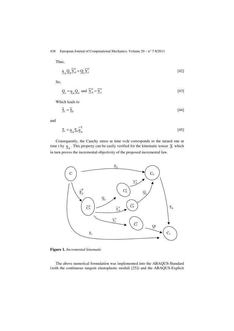
To prove the incremental objectivity of this algorithm, we consider that the

increment of deformation gradient is an arbitrarily increment of rotation (orthogonal

tensor ∆∆ = qF ). Figure 1 gives the incremental kinematic in this case, where C

denotes rotated configurations, the superscripts e and p over C states respectively for

elastic and plastic configurations. From this figure we can write

p

0

e

11

p

0

e

00

p

00

e01 FVQFVQqFQVqF ===

∆∆ [41]


Thus,

e

11

e

00VQVQq =

∆ [42]

So,

01QqQ

∆= and

e

1

e

0 VV = [43]

Which leads to

01 ττ = [44]

and

T

01 qq∆∆

ττ = [45]

Consequently, the Cauchy stress at time t+∆t corresponds to the turned one at

time t by ∆

q . This property can be easily verified for the kinematic tensor X which

in turn proves the incremental objectivity of the proposed incremental law.

Figure 1. Incremental kinematic

The above numerical formulation was implemented into the ABAQUS-Standard

(with the continuous tangent elastoplastic moduli [25]) and the ABAQUS-Explicit

P

0F

C C0

p0C

e0C

∆q

0Q

0Q

e

0V

e

0V

0F

e0C

1F

e

1V

1Q

e1C

C1


using, respectively, the implicit user subroutine UMAT and the explicit user

subroutine VUMAT.

4. Application to some sheet metal forming processes

The main goals of the following numerical tests are, firstly, to check the

accuracy of the integration algorithm, and secondly, to show that the implemented

model takes into account the important aspects of isotropic and kinematic hardening.

4.1. Application to the RVE: Parametric study of the integration algorithms

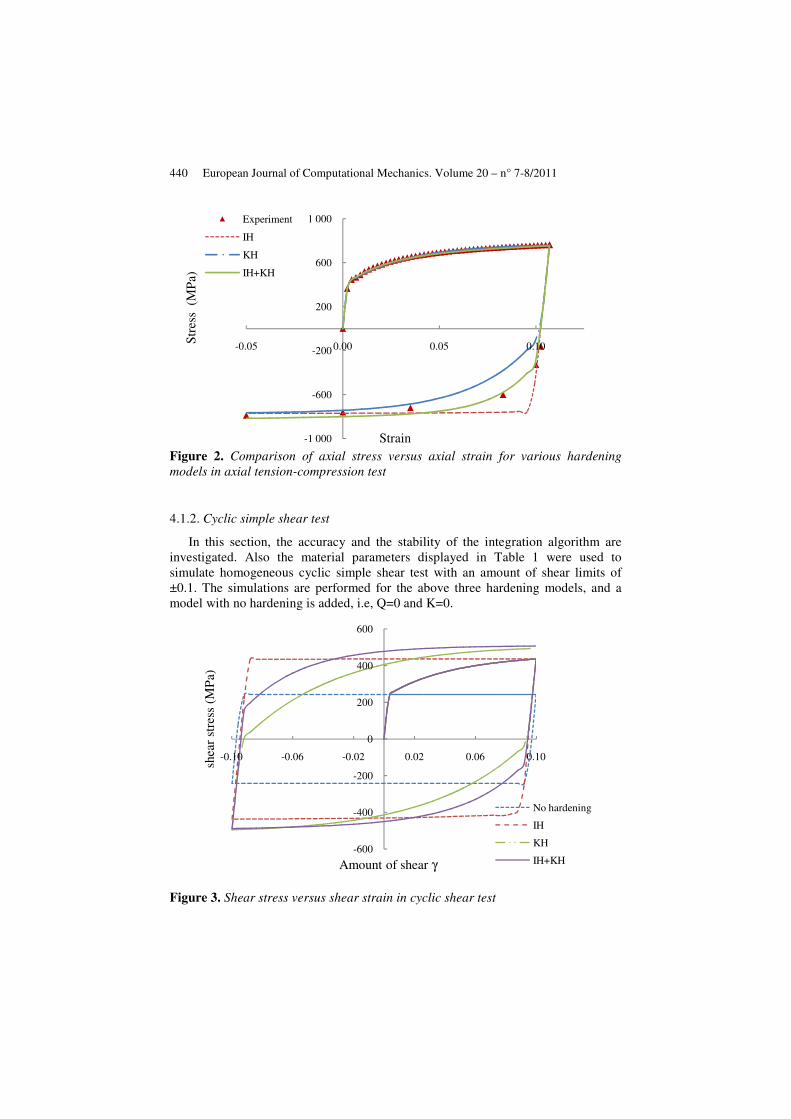
4.1.1. Monotonic and cyclic tension

Stress–strain data obtained experimentally (Taherizadeh et al., 2009) will be

compared with numerical results obtained by the use of the following three

hardening models: (i) isotropic hardening: IH; (ii) kinematic hardening: KH; and

(iii) combined isotropic and kinematic hardening: IH+KH. Table 1 gives the

material parameters of the DP600 steel used in the following numerical simulations.

A fixed time step of ∆t=0.01 s was adopted. Figure 2 shows that when the isotropic

hardening is only used, an increase in the axial stress is observed, and the initial

flow stress level obtained from both tension and compression are equal in

magnitude. In the case of the KH law, it is again observed an increase in the axial

stress, but the magnitude of the initial flow stress level in compression path is

significantly smaller than the flow stress level in tension; a clear expression of the

Bauschinger effect. When the IH is combined with kinematic hardening (IH+KH), it

can be seen that there are again a clear Bauschinger effect upon strain reversal and it

is clear that this model gives the best numerical results when compared with the

experimental data.

Table1. Material parameters of the DP 600 steel

Voce law IH Kinematic KH Combined (IH+KH)

Q=318 Mpa

b=30

K=9500 Mpa

γ=30

Q=200 Mpa

b=8

K=9500 Mpa

γ=50

Hill’48 parameters Elastic properties Initial yield stress

F=0.438

G=0.462

H=0.535

L=M=1.5

N=1.822

E=210 GPa

ν=0.3

σ0=420 Mpa


Figure 2. Comparison of axial stress versus axial strain for various hardening models in axial tension-compression test

4.1.2. Cyclic simple shear test

In this section, the accuracy and the stability of the integration algorithm are

investigated. Also the material parameters displayed in Table 1 were used to

simulate homogeneous cyclic simple shear test with an amount of shear limits of

±0.1. The simulations are performed for the above three hardening models, and a

model with no hardening is added, i.e, Q=0 and K=0.

Figure 3. Shear stress versus shear strain in cyclic shear test

-1 000

-600

-200

200

600

1 000

-0.05 0.00 0.05 0.10

Str

ess

(M

Pa)

Strain

Experiment

IH

KH

IH+KH

-600

-400

-200

0

200

400

600

-0.10 -0.06 -0.02 0.02 0.06 0.10

shea

r st

ress

(M

Pa)

Amount of shear γ

No hardening

IH

KH

IH+KH


Figure 3 shows the important qualitative aspects of each case in cyclic simple

shear, i.e. elastic-perfectly-plastic response in the case of no hardening, a continual

increase in the flow stress in cases involving isotropic hardening, and a clear

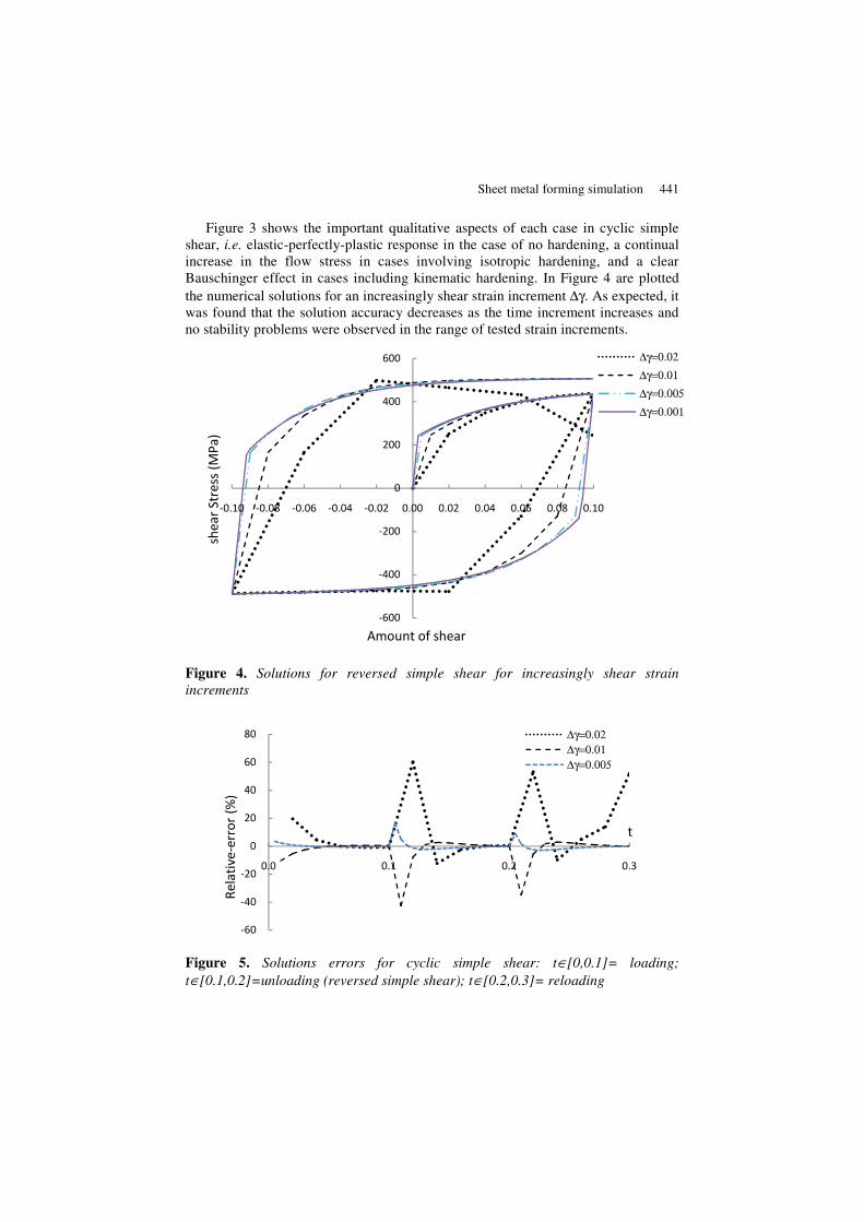
Bauschinger effect in cases including kinematic hardening. In Figure 4 are plotted

the numerical solutions for an increasingly shear strain increment ∆γ. As expected, it

was found that the solution accuracy decreases as the time increment increases and

no stability problems were observed in the range of tested strain increments.

Figure 4. Solutions for reversed simple shear for increasingly shear strain increments

Figure 5. Solutions errors for cyclic simple shear: t∈[0,0.1]= loading; t∈[0.1,0.2]=unloading (reversed simple shear); t∈[0.2,0.3]= reloading

-600

-400

-200

0

200

400

600

-0.10 -0.08 -0.06 -0.04 -0.02 0.00 0.02 0.04 0.06 0.08 0.10

she

ar

Str

ess

(M

Pa

)

Amount of shear

∆γ=0.02

∆γ=0.01

∆γ=0.005

∆γ=0.001

-60

-40

-20

0

20

40

60

80

0.0 0.1 0.2 0.3

Re

lati

ve

-err

or

(%)

t

∆γ=0.02

∆γ=0.01

∆γ=0.005


In Figure 5 are plotted a relative-error parameter based on the following shear

difference

Relative-error (%) = 100exact

numexact

τ

τ−τ [46]

where τnum is the numerical shear stress and τexact is the exact one. Since no exact

solution is available, the solution obtained using a time step of ∆γ=10-3

was

considered as the exact solution. Again, Figure 4 shows that the results accuracy

decreases for increasingly time increments, especially at stress-strain reversals.

4.2. Application to some sheet metal forming processes

4.2.1. Hydro bulging test

The hydraulic bulging test is schematically represented in Figure 6. Table 2

gives the material parameters of the 2008-T4 aluminum alloy used in this test. The

geometry dimensions are given as follows: blank radius of 81 mm; die radius of 12.7

mm and the sheet thickness of 1.24 mm. Note that the specific dimensions of the

tools and process parameters as well as the material properties were given in (De

Sousa et al., 2007; Chung and Shah, 1992). The implicit FE simulations (UMAT in

Abaqus Standard) were conducted using shell elements with 5 Gauss points through

the thickness direction. Only a quarter section of the specimen was considered due

to the orthotropic material symmetry.

Table 2. Material parameters of 2008-T4 aluminum alloy

Voce law IH

R(p) = 185+223(1-e-6.14p

) MPa

Initial yield stress

σ0=185 MPa

Hill’48 parameters

F=0.764

G=0.541

H=0.459

L=M=N=1.584

Elastic properties

E=69 GPa

ν=0.33

Figure 6. Schematic illustration of the hydraulic bulge test

p h

Die

Blank

Holder


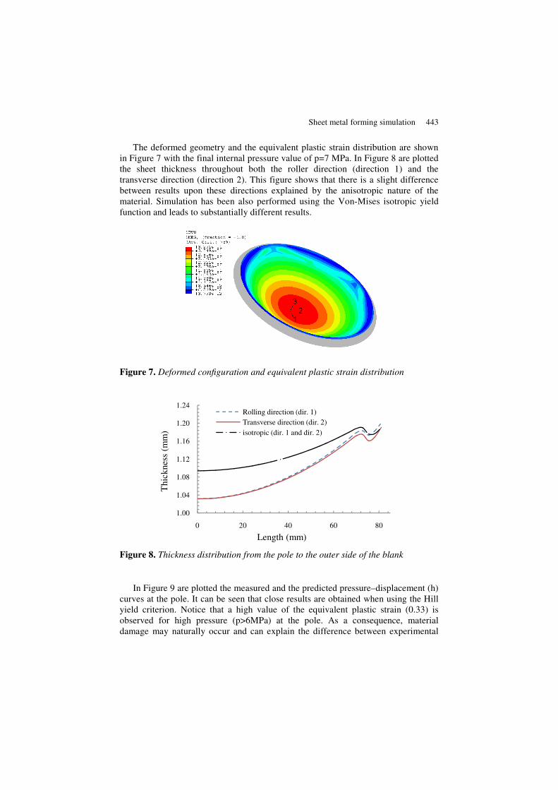
The deformed geometry and the equivalent plastic strain distribution are shown

in Figure 7 with the final internal pressure value of p=7 MPa. In Figure 8 are plotted

the sheet thickness throughout both the roller direction (direction 1) and the

transverse direction (direction 2). This figure shows that there is a slight difference

between results upon these directions explained by the anisotropic nature of the

material. Simulation has been also performed using the Von-Mises isotropic yield

function and leads to substantially different results.

Figure 7. Deformed configuration and equivalent plastic strain distribution

Figure 8. Thickness distribution from the pole to the outer side of the blank

In Figure 9 are plotted the measured and the predicted pressure–displacement (h)

curves at the pole. It can be seen that close results are obtained when using the Hill

yield criterion. Notice that a high value of the equivalent plastic strain (0.33) is

observed for high pressure (p>6MPa) at the pole. As a consequence, material

damage may naturally occur and can explain the difference between experimental

1.00

1.04

1.08

1.12

1.16

1.20

1.24

0 20 40 60 80

Thic

knes

s (m

m)

Length (mm)

Rolling direction (dir. 1)

Transverse direction (dir. 2)

isotropic (dir. 1 and dir. 2)


and simulated results for elevated pressure values. Consequently, elastoplastic

model coupled with damage should be used.

Figure 9. Polar displacement vs. hydraulic pressure

4.2.2. Deep drawing test

In order to experiment the implemented material model in more complicated

forming processes, a cylindrical deep cup drawing is simulated. This test is

schematically presented in Figure 10 and specific tool dimensions are listed in

Table 3. The used material is the Al2090-T3 and its parameters are displayed in

Table 4.

Figure 10. Cup drawing setup

Note that this test is one of the forming operations where the effects of the

yielding anisotropy are most evident. After forming, the profile of the drawn cup is

not uniform, but shows a series of ears. The simulations were conducted using shell

element with 5 integration points through the thickness direction. Due to the

material orthotropy, only a quarter section of the cup was treated. Figure 11 shows

0

1

2

3

4

5

6

7

0 10 20 30 40

P(M

Pa)

h(mm)

Experiment

Anisotropic

Isotropic


the finite element mesh with 456 shell elements for the quarter section of the cup.

The die, punch and blank holder are all defined as rigid tools.

Table 3. Geometrical data for the cup drawing test

Punch diameter

Punch profile radius

Die opening diameter

Die profile radius

Blank diameter

Initial sheet thickness

friction coefficient

Blank holding force

Dp =97.46 mm

rp = 12.70 mm

Dd = 101.48 mm

rd = 12.70 mm

Db = 158.76 mm

t0=1.6 mm

0.1

22.2 KN

Table 4. Material parameters of Al2090-T3

Isotropic law (Swift) Kinematic law

C=646 MPa

ε0=0.025

n=0.227

K=300 MPa

γ=5

Hill’48 parameters

F=0.5702

G=0.3632

H=0.6368

L=M=N=2.57

Elastic properties

E0=69 GPa

ν=0.33

Initial yield stress

σ0=276.6 MPa

Figure 11. Element meshing of one quarter of circular sheet (1: Rolling direction; 2: Transverse direction)


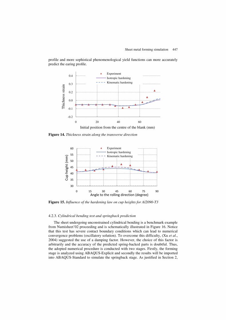
Figure 12 shows the deformed configuration of the fully drawn cup. It can be

seen that four ears are obtained which agree with (Youn et al., 2000)’s results.

Figure 13 shows that the thickness strain distribution in the rolling direction is in

good agreement with the experimental result. However, Figure 14 shows that the

thickness strain distribution in the transverse direction deviates from the simulated

result at the outer side of the blank.

Figure 12. Deformed shape and Von-Mises stress contour of fully-drawn cup

Figure 13. Thickness strain along the rolling direction

In Figure 15 are plotted the measured and the predicted cup height profiles

between 0° and 90°. This figure shows that the magnitude of the earing profile

obtained numerically deviates from the experimental result, especially around 45°.

Note that a slight improvement is observed when using the kinematic hardening. It

is reported by (Yoon et al., 2000) that the prediction of both earing amplitude and

location of ears depend strongly on the used yield function. As a result, usual

anisotropic yield criteria are not able to provide an accurate prediction of the earing

-0.2

-0.1

0.0

0.2

0.3

0.4

0 20 40 60

Th

ich

ne

ss s

tra

in

Initial position from the centre of the blank (mm)

Experiment

Isotropic hardening

Kinematic hardening


profile and more sophistical phenomenological yield functions can more accurately

predict the earing profile.

Figure 14. Thickness strain along the transverse direction

Figure 15. Influence of the hardening law on cup heights for Al2090-T3

4.2.3. Cylindrical bending test and springback prediction

The sheet undergoing unconstrained cylindrical bending is a benchmark example

from Numisheet’02 proceeding and is schematically illustrated in Figure 16. Notice

that this test has severe contact boundary conditions which can lead to numerical

convergence problems (oscillatory solution). To overcome this difficulty, (Xu et al., 2004) suggested the use of a damping factor. However, the choice of this factor is

arbitrarily and the accuracy of the predicted spring-backed parts is doubtful. Thus,

the adopted numerical procedure is conducted with two stages. Firstly, the forming

stage is analyzed using ABAQUS-Explicit and secondly the results will be imported

into ABAQUS-Standard to simulate the springback stage. As justified in Section 2,

-0.2

-0.1

0.0

0.2

0.3

0.4

0 20 40 60

Thic

hnes

s st

rain

Initial position from the centre of the blank (mm)

Experiment

Isotropic hardening

Kinematic hardening

30

35

40

45

50

55

60

0 15 30 45 60 75 90

Cu

p h

eig

ht

(mm

)

Angle to the rolling direction (degree)

Experiment

Isotropic hardening

Kinematic hardening


the implemented elastic-plastic model uses the hypoelastic law [13] in forming

stage, while, in springback stage, the elastic law [11] is used.

The sheet dimensions are length of 120 mm, width of 30 mm and thickness of 1

mm. The material used is the 6111-T4 aluminum alloy with material parameters

given in Table 5. Notice that the specific dimensions of the tools and process

parameters as well as the material proprieties were given in (Yoon et al., 2002).

Figure 16. Problem setup and dimensions of the unconstrained cylindrical bending test

Table 5. Material parameters of the 6111-T4 aluminum alloy

Young’s modulus (GPa) 70

Poisson’s ration 0.3

Hardening law (MPa) R(p) = 192.1+237.7(1-e-8.504p)

Numerical simulations are carried out using plane strain elements with

4 elements through the sheet thickness. Due to the material symmetry, only a half

section of the blank was analyzed. Finite element mesh used for the analysis is

composed of 480 plane strain elements (CPE4R) for the half section of the blank.

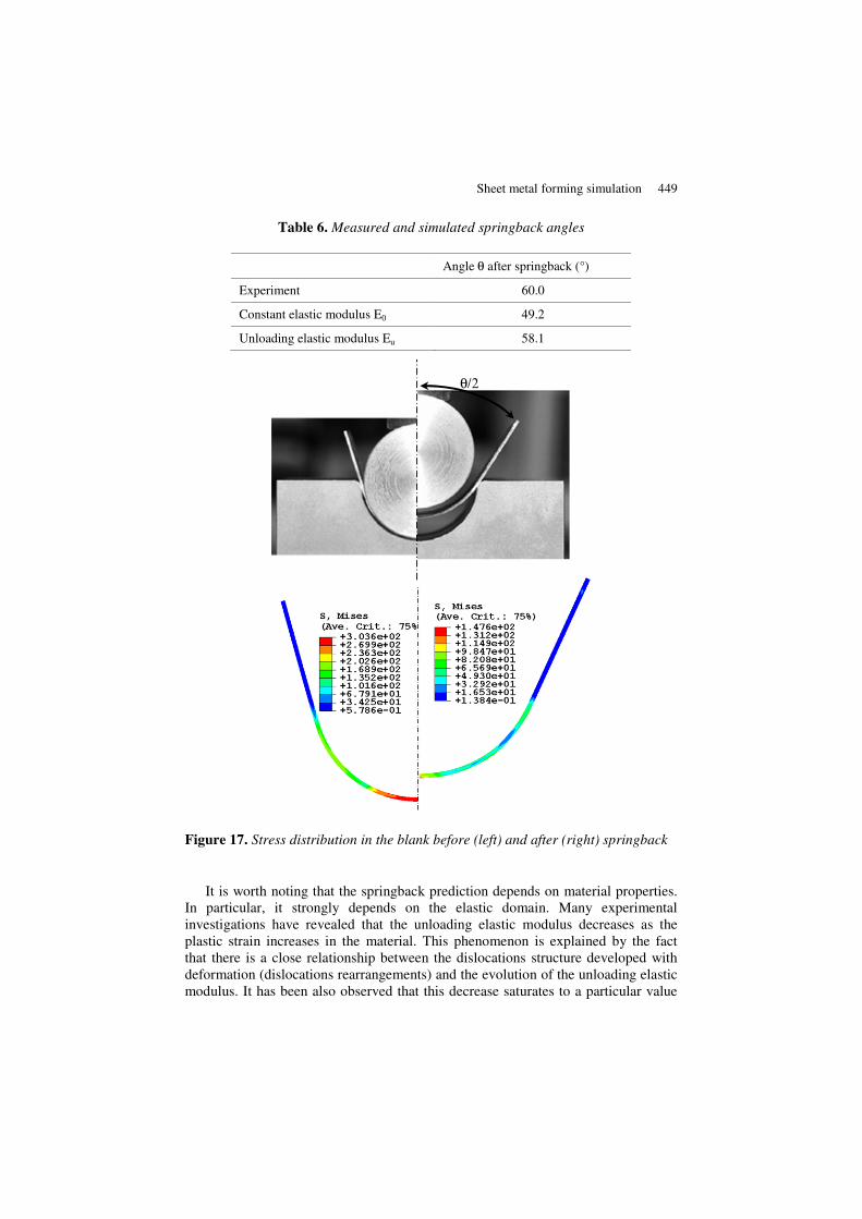
Figure 17 gives the equivalent stress distribution in the sheet before and after

springback. Table 6 shows that significant difference is observed between the

experimental springback angle and the predicted one especially when considering

constant unloading elastic modulus (E0). Notice that the angle reached just before

springback stage was 32.9° found by Ferreira et al. (2006) by a computer vision

based method.


Table 6. Measured and simulated springback angles

Angle θ after springback (°)

Experiment 60.0

Constant elastic modulus E0 49.2

Unloading elastic modulus Eu 58.1

Figure 17. Stress distribution in the blank before (left) and after (right) springback

It is worth noting that the springback prediction depends on material properties.

In particular, it strongly depends on the elastic domain. Many experimental

investigations have revealed that the unloading elastic modulus decreases as the

plastic strain increases in the material. This phenomenon is explained by the fact

that there is a close relationship between the dislocations structure developed with

deformation (dislocations rearrangements) and the evolution of the unloading elastic

modulus. It has been also observed that this decrease saturates to a particular value

θ/2


after some amount of plastic prestrain. Both polynomial (Yu, 2009) and exponential

(Yoshida et al., 2002) expressions were used in order to model this phenomenon. In

this study, the widely used exponential expression is considered

Eu=E0-(E0-Ea)[1-exp(-ξ p0ε )] [47]

where E0 is the initial elastic modulus, Ea is the decreased elastic modulus obtained

for infinitely large prestrained material, p0ε is the equivalent plastic pre-strain

reached just before the unloading stage, and ξ is a material constant which

determines the rate of the elastic modulus decrease.

A modified formula has been proposed by (Chatti and Hermi, 2011) that gives

non linear unloading behaviour (non linear recovery experimentally observed in

tensile tests) in order to obtain more accurate results in springback simulations.

(Cleveland and Ghosh, 2002) reported that the elastic modulus can lose 19% of its

value for high strength steel and 11% for the AA6022-T4 aluminum alloy for only

7% of plastic strain. Accordingly, the unloading elastic parameters of the 6111-T4

aluminum alloy, whose properties are similar to those of AA6022-T4, are displayed

in Table 7.

Figure 18. Distribution of the elastic modulus (left) and the equivalent plastic strain (right) in the unloaded sheet

Table 7. Properties of the unloading elastic modulus

E0 Ea ξ

70 GPa 61 GPa 120

In the following simulations, the elastic modulus is taken to be constant in

loading phase as suggested by (Ghaei et al., 2010), whereas, in springback

simulations, the unloading modulus is reduced according to Equation [47]. It can be


easily shown that the elastoplastic tangent modulus [27] in springback simulation

reduces to the elastic moduli tensor e

C .

Figure 18 gives the elastic modulus and the equivalent plastic strain contours in

the unloaded sheet. Notice that the highest value of the equivalent plastic strain is

0.085 which is generally a small value and no material damage can occur. Table 6

gives the springback angle using the unloading elastic modulus [47]. It is clear that

there is a significant improvement in springback prediction when compared to the

experiment. These results allow concluding that, in order to obtain accurate

springback predictions in sheet metal forming processes, the elastic modulus

decrease have to be considered.

5. Conclusions and main perspectives

The anisotropic elastoplastic behavior which accounts for non-linear

isotropic/kinematic hardening under large deformations was presented. Elasticity

was modeled by both:

– hypoelastic formulation used in loading phases (forming);

– elastic formulation used in elastic processes (elastic predictor or springback).

An incremental formulation was developed for the integration of the constitutive

equations. In this study, only Hill’s yield criterion was considered. However, the

proposed integration algorithm is quite general and can be used with any yield

function. User material subroutines (UMAT and VUMAT) were developed for both

ABAQUS-Standard and ABAQUS-Explicit. Simulations were carried out using

several hardening models. It was found that, due to its ability to model the

Bauschinger effect, the combined non-linear isotropic/kinematic model gives results

which agree with experiment in cyclic simple tests. The accuracy of the

implemented material model was also verified through the hydraulic bulge test.

However, it was found that in the cylindrical cup drawing test the numerical results

slightly deviate from experimental data. Nevertheless, it would appear that

numerical results can be further improved by implementing more advanced yield

functions; we leave such work to the future. Finally, the unconstrained cylindrical

bending of Numisheet’02 benchmark including springback was simulated by using

both explicit (for loading) and implicit (for unloading) simulations. The unloading

elastic modulus decrease with plastic prestrain was taken into account in the

implemented model and better springback prediction was obtained. However, the

hysteresis phenomenon, observed in elastic evolution (unloading/reloading), should

be taken into account in the behavior law. In addition, for highly loaded parts,

coupled damage model have to be taken into account in order to consider the

degradation of the elastic modulus which may strongly affect springback prediction.

It can be concluded that the proposed numerical algorithm is sweetable for the

simulation of sheet metal forming processes including springback.


References

Badreddine H., Saanouni K., Dogui A., “On non-associative anisotropic finite plasticity fully

coupled with isotropic ductile damage for metal forming”, International Journal of Plasticity, 26, 2010, p. 1541-1575.

Chatti S., Hermi N., “The effect of non-linear recovery on springback prediction”, Computers and Structures, 89, 2011, p. 1367-1377.

Chatti S., “Effect of the elasticity formulation in finite strain on springback prediction”,

Computers and Structures, 88, 2010, p. 796-805.

Chatti S., Dogui A., Dubujet P., Sidoroff F., “An objective incremental formulation for the

solution of anisotropic elastoplastic problems at finite strain”, Communication in Num. Methods in Engeneering, 17, 2010, p. 845-862.

Chung K., Shah K., “Finite element simulation of sheet metal forming for planar anisotropic

metals”, International Journal of Plasticity, 8, 1992, p. 453-476.

Cleveland R.M., Ghosh A. K., “Inelastic effects on springback in metals”, International Journal of Plasticity, 18, 2002, p. 769-785.

De Sousa R.J. A., Yoon J.W., Cardoso R. P. R., Valente R. A. F., Gràcio J.J., “On the use of a

reduced enhanced solid-shell (RESS) element for sheet forming simulations”,

International Journal of Plasticity, 23, 2007, p. 490-515.

Dogui A., « Cinématique bidimensionnelle en grandes déformations – Application à la

traction hors axes et à la torsion », Journal de Mécanique Théorique et Appliquée, 7,

1988, p. 43-64.

Ferreira J.A., Sun P., Grácio J.J., “Close loop control of a hydraulic press for springback

analysis”, Journal of Materials Processing Technology, 177, 2006, p. 377-381.

Ghaei A., Green D.E., Taherizadeh A., Semi-implicit numerical integration of Yoshida–

Uemori two-surface plasticity model, International Journal of Mechanical Sciences, 52,

2010, p. 531-540.

Huges T.J.R., Winget T. J., “Finite rotation effects in numerical integration of rate

constitutive equations arising in large-deformation analysis”, Int. J. for Numer. Meth. in Eng., 15, 1980, p. 1862-1867.

Ingarao G., Di Lorenzo R., “A new progressive design methodology for complex sheet metal

stamping operations: Coupling spatially differentiated restraining forces approach and

multi-objective optimization”, Computers and Structures, 88, 2010, p. 625-638.

Laurent H., Grèze R., Oliveira M. C., Menezes L. F., Manach P.Y., Alves J. L., “Numerical

study of springback using the split-ring test for an AA5754 aluminum alloy”, Finite Elements in Analysis and Design, 46, 2010, p. 751-759.

Lemaître J., Chaboche J.L., Mécanique des matériaux solides, Dunod Eds, Paris, 1985.

Mandel J., « Equations constitutives et directeurs dans les milieux plastiques et

viscoplastiques », International Journal of solids and structures, 9, 1971, p. 725-740.


Nagtegaal J. C., Dejong J.E., “Some computational aspects of elastic-plastic large strain

analysis”, International journal of numerical methods in engineering, 17, 1981, p. 15-41.

Ortiz M., Simo J.C., “An analysis of a new class of integration algorithms for elastoplastic

relations”, International Journal of Numerical Methods in Engineering, 23, 1986.

Ortiz R., Popov E.P., “Accuracy and stability of integration algorithms for elastoplastic

constitutive relations”, International Journal for numerical methods and engineering, 21,

1985, p. 1561-1576.

Sidoroff F., Dogui A., “Some issues about anisotropic elastic-plastic models at finite strain”,

International Journal of solids and structures, 38, 2001, p. 9569-9578.

Sidoroff F., « Lois incrémentales en MMC grandes déformations », 10e Congrés Français de Mécanique, Paris, septembre, 1991.

Taherizadeh A., Green D. E., Ghaei A., Yoon J.W., “A non-associated constitutive model

with mixed iso-kinematic hardening for finite element simulation of sheet metal forming”,

International Journal of Plasticity 26, 2009, p. 288-309.

Xu W.L., C. H. Ma, C.H. Li and W.J. Feng, “Sensitive factors in springback simulation for

sheet metal forming”, Journal of Materials Processing Technology, 151, 2004, p. 217-

222.

Yoon J.W., Pourboghrat F., Chung K., Yang D.Y., Springback prediction for sheet metal

forming process using a 3D hybrid membrane/shell method, International Journal of Mechanical Sciences, 44, 2002, p. 2133-2153.

Yoon J.W., Barlat F., Chung K., Pourboghrat F., Yangn D.Y., “Earing predictions based on

asymmetric non-quadratic yield function”, International Journal of Plasticity, 16, 2000,

p. 1075-1104.

Yoshida F., Uemori T., Fujiwara K., “Elastic-plastic behavior of steel sheets under in-plane

cyclic tension-compression at large strain”, International Journal of Plasticity, 18, 2002,

p. 633-659.

Yu H. Y., “Variation of elastic modulus during plastic deformation and its influence on

springback”, Materials and Design, 30, 2009, p. 846-850.

Received: 28 April 2011 Accepted: 6 January 2012

Sheet metal forming simulation using finite elastoplasticity with mixed isotropic/kinematic...

Documents

Transcript of Sheet metal forming simulation using finite elastoplasticity with mixed isotropic/kinematic...