THE HARDENING SOIL MODEL - A PRACTICAL GUIDEBOOK
216
THE HARDENING SOIL MODEL - A PRACTICAL GUIDEBOOK Z Soil.PC 100701 report revised 21.10.2018 by Rafa l F. Obrzud Andrzej Truty Edition 2018 Zace Services Ltd, Software engineering P.O.Box 224, CH-1028 Pr´ everenges Switzerland (T) +41 21 802 46 05 (F) +41 21 802 46 06 http://www.zsoil.com, hotline: [email protected] since 1985
-
Upload
khangminh22 -
Category
Documents
-
view
0 -
download
0
Transcript of THE HARDENING SOIL MODEL - A PRACTICAL GUIDEBOOK
THE HARDENING SOIL MODEL -A PRACTICAL GUIDEBOOKZ Soil.PC 100701 reportrevised 21.10.2018
byRafa l F. ObrzudAndrzej Truty
Edition 2018
Zace Services Ltd, Software engineering
P.O.Box 224, CH-1028 Preverenges
Switzerland
(T) +41 21 802 46 05
(F) +41 21 802 46 06
http://www.zsoil.com,
hotline: [email protected]
since 1985

Contents
Table of Contents 1
List of symbols 9
FAQ’s 11
1 Introduction 1
1.1 Why do we need the HS-SmallStrain model? . . . . . . . . . . . . . . . . . 2
1.2 Application fields of constitutive models . . . . . . . . . . . . . . . . . . . . 6
2 Short introduction to the HS models 11
2.1 Hardening Soil-Standard model . . . . . . . . . . . . . . . . . . . . . . . . 13
2.1.1 Shear mechanism . . . . . . . . . . . . . . . . . . . . . . . . . . . 13
2.1.1.1 Shear yield mechanism . . . . . . . . . . . . . . . . . . . 13
2.1.2 Stress dependent stiffness . . . . . . . . . . . . . . . . . . . . . . . 15
2.1.2.1 Stress dependent stiffness based on the mean effective stress. 17
2.1.2.2 Parameter migration between minor and mean stress formu-lations . . . . . . . . . . . . . . . . . . . . . . . . . . . . 18
2.1.2.2.1 Integrated tool for moduli migration . . . . . . . 22
2.1.3 Shear hardening law . . . . . . . . . . . . . . . . . . . . . . . . . . 23
2.1.4 Plastic flow rule and dilatancy . . . . . . . . . . . . . . . . . . . . . 24
2.1.5 Volumetric mechanism . . . . . . . . . . . . . . . . . . . . . . . . . 27
2.1.6 Additional strength criterion . . . . . . . . . . . . . . . . . . . . . . 29
2.1.7 Initial state variables . . . . . . . . . . . . . . . . . . . . . . . . . . 30
2.1.8 Troubleshooting for Initial State analysis . . . . . . . . . . . . . . . 34
2.2 Hardening Soil-SmallStrain model . . . . . . . . . . . . . . . . . . . . . . . 35
2.2.1 Non-linear elasticity for small strains . . . . . . . . . . . . . . . . . 35
2.2.2 Modifications of the plastic part . . . . . . . . . . . . . . . . . . . . 37
2.3 Model parameters . . . . . . . . . . . . . . . . . . . . . . . . . . . . . . . 43
3 Parameter determination 47
3.1 Experimental testing requirements for direct parameter identification . . . . 48
3.1.1 Direct parameter identification for the Hardening-Soil Standard . . . 48
3.1.2 Direct parameter identification for the Hardening-Soil Small . . . . . 55
3.1.3 Parameter identification sequence . . . . . . . . . . . . . . . . . . . 56
3.1.4 Model parameters for ”undrained” simulations . . . . . . . . . . . . 57
3.2 Alternative parameter estimation for granular materials . . . . . . . . . . . . 59
3.2.1 Initial stiffness modulus and small strain threshold . . . . . . . . . . 59
3.2.2 Secant and unloading-reloading moduli . . . . . . . . . . . . . . . . 71
3.2.3 Oedometric modulus . . . . . . . . . . . . . . . . . . . . . . . . . . 76
3.2.4 Unloading-reloading Poisson’s ratio . . . . . . . . . . . . . . . . . . 78
3.2.5 Stiffness exponent . . . . . . . . . . . . . . . . . . . . . . . . . . . 79
3.2.6 Friction angle . . . . . . . . . . . . . . . . . . . . . . . . . . . . . 81
3.2.7 Dilatancy angle . . . . . . . . . . . . . . . . . . . . . . . . . . . . 86
3.2.8 Coefficient of earth pressure ”at rest” . . . . . . . . . . . . . . . . . 87
3.2.9 Void ratio . . . . . . . . . . . . . . . . . . . . . . . . . . . . . . . 88
3.2.10 Overconsolidation ratio . . . . . . . . . . . . . . . . . . . . . . . . 90
3.2.11 Coefficient of earth pressure ”at rest” . . . . . . . . . . . . . . . . . 91
3.3 Alternative parameter estimation for cohesive materials . . . . . . . . . . . . 92
3.3.1 Initial stiffness modulus and small strain threshold . . . . . . . . . . 92
3.3.2 Strength parameters . . . . . . . . . . . . . . . . . . . . . . . . . 102
3.3.3 Failure ratio . . . . . . . . . . . . . . . . . . . . . . . . . . . . . . 106
3.3.4 Dilatancy angle . . . . . . . . . . . . . . . . . . . . . . . . . . . . 107
3.3.5 Stiffness moduli . . . . . . . . . . . . . . . . . . . . . . . . . . . . 108
3.3.6 Oedometric modulus . . . . . . . . . . . . . . . . . . . . . . . . . . 114
3.3.7 Stiffness exponent . . . . . . . . . . . . . . . . . . . . . . . . . . . 116
3.3.8 Overconsolidation ratio . . . . . . . . . . . . . . . . . . . . . . . . 118
3.3.9 Coefficient of earth pressure ”at rest” . . . . . . . . . . . . . . . . . 121
3.3.10 Void ratio . . . . . . . . . . . . . . . . . . . . . . . . . . . . . . . 126
3.4 Automated assistance in parameter determination . . . . . . . . . . . . . . 127
4 Benchmarks 129
4.1 Triaxial drained compression test on dense Hostun sand . . . . . . . . . . . 129
4.2 Isotropic compression of dense Hostun sand . . . . . . . . . . . . . . . . . . 133
4.3 Oedometric compression test . . . . . . . . . . . . . . . . . . . . . . . . . 134

4.4 Oedometric compression test - KNC0 -path test . . . . . . . . . . . . . . . . 135
5 Case studies 137
5.1 Excavation in Berlin Sand . . . . . . . . . . . . . . . . . . . . . . . . . . . 137
5.2 Twin tunnels excavation in London Clay . . . . . . . . . . . . . . . . . . . 145
5.3 Spread footing on overconsolidated Sand . . . . . . . . . . . . . . . . . . . 161
A Determination of undrained shear strength 179
A.1 Non-uniqueness of undrained shear strength . . . . . . . . . . . . . . . . . . 179
A.2 Determination of su from field tests . . . . . . . . . . . . . . . . . . . . . . 181
B Estimation of compression index 183
C Estimation of shear wave velocity 187
References 205


List of Symbols
Stress and Strain Notationε strain
εv volumetric strain= (ε1 + ε2 + ε3)
γs shear strain
σ stress
τ shear stress
p total mean stress= 1
3 (σ1 + σ2 + σ3)
p′ mean effective stress
q deviatoric stress= 1√
2[(σ1 − σ2)2 +
+ (σ2 + σ3)2 + (σ3 − σ1)2]1/2
Roman Symbolssu undrained shear strength
E0 maximal soil stiffness
e0 initial void ratio
Eoed tangent oedometric modulus
E50 secant modulus corresponding to50% of qf
Eur unloading-reloading stiffness
G0 (orGmax) maximal small-strain shearmodulus
K0 coefficient of in situ earth pres-sure at rest (K0 > KNC
0 for OCR >1)
KNC0 coefficient of earth pressure at rest
of normally-consolidated soil
KSR0 stress reversalK0 coefficient defin-
ing stress point position at inter-section between hardening mech-anisms
qPOP (=σ′v0 + σ′c) preoverburden pres-sure
Bq pore pressure parameter for CPTU
c cohesion intercept
c∗ intercept for M∗ slope in q − p′plane (=6c cosφ/(3− sinφ))
Cc slope of the normal compressionline in log10 scale (=2.3λ)
Ck coefficient of curvature (=d230/(d10·d60)
CN overburden correction factor forSPT N60-value
Cr slope of unload-reload consolida-tion line in log10 scale
Cu coefficient of uniformity (=d60/d10)
D scaling parameter (by default =1.0for HS-Std, =0.25 for HS-SmallStrain)
Dr relative density
E Young’s modulus
e void ratio
ED dilatometer modulus (= 34.7(p1−p0))
emax maximal void ratio
ft limit tensile strength
G tangent shear modulus
Gur unload-reload shear modulus
Gs secant shear modulus
H parameter which defines the rateof the volumetric plastic strain
ID dilatometer material index (= (p1−p0)/(p0 − u0))
IP plasticity index (= wL − wP )
KD dilatometer horizontal stress in-dex (= (p0 − u0)/σ′v0)
M parameter of HS model which de-fines the shape of the cap surface
m stiffness exponent for minor stressformulation
M∗ (or M∗c ) slope of critical state line(= 6 sinφ′c/(3− sinφ′c))
M∗e slope of critical state line (= 6 sinφ′c/(3+sinφ′c))
MDMT constrained modulus derived fromthe Marchetti’s dilatometer
MD one-dimensional drained constrainedmodulus

mp stiffness exponent for p′-formulation
p0 corrected first DMT reading
p1 corrected second DMT reading
pa atmospheric pressure (average sea-level pressure is 101.325 kPa)
pc effective preconsolidation pressurein terms of mean stress
pco initial effective preconsolidation pres-sure
qa asymptotic deviatoric stress
qc cone resistance
qf deviatoric stress at failure
Qt normalized cone resistance for CPT
qt corrected cone resistance
Rf failure ratio (= qf/qa)
u pore pressure
Vs shear wave velocity
wL liquid limit
wn water content
wP plastic limit
z depth
OCR overconsolidation ratio (= σ′c/σ′vo)
PI plasticity index
Greek SymbolsγPS plastic strain hardening parame-
ter for deviatoric mechanism
γSAT saturated unit weight
γD dry unit weight
γs shear strain
γw water unit weight
γ0.7 value of small strain for whichGs/G0
reduces to 0.722
κ slope of unload-reload consolida-tion line in ln scale
Λ plastic volumetric strain ratio (=1− κ/λ)
λ slope of primary consolidation linein ln scale
ν Poisson’s coefficient
νur unloading/reloading Poisson’s co-efficient
φ friction angle
φ′c effective friction angle from com-pression test
φ′e effective friction angle from ex-tension test
φ′cs critical state friction angle
φ′m mobilized friction angle
φ′tc effective friction angle determinedfrom triaxial compression test
ψ dilatation angle
ψm mobilized dilatation angle
ρ soil density
σref reference stress
σ′c effective vertical preconsolidationstress
σL minimal limit minor stress
AbbreviationsCKoUC Ko consolidated undrained com-
pression
CKoUE Ko consolidated undrained exten-sion
CAP Cap model with Drucker-Pragerfailure criterion
CIDC consolidated isotropic drained com-pression
CIUC consolidated isotropic undrainedcompression
CIUE consolidated isotropic undrainedextension
CPTU cone penetration test with porepressure measurements (electric piezo-cone)
CSL critical state line
DMT Marchetti dilatometer test
DSS direct simple shear
FVT field vane test
MC Mohr-Coulomb model
MCC Modified Cam clay model
NCL normal consolidation line
OED oedometric test
PMT pressuremeter test
SBPT self-boring pressuremeter test
SCPT static penetration test with seis-mic sensor
SLS serviceability limit state analysis
SPT standard penetration test
TC triaxial compression
UCS unified classification system
ULS ultimate limit state analysis

Sign convention: Throughout this report, the
sign convention is the standard convention of
soil mechanics, i.e. compression is assigned as
positive.

FAQs
1. When should the HS model be applied and what are its advantages?
2. Which formulation to describe the stress dependent stiffness should be chosen?
3. How to migrate stiffness moduli between two different formulations for stress dependentstiffness?
4. How to set model parameters for an ”undrained” simulation?
5. How to troubleshoot convergence problem at the initial state analysis?
6. What is a typical ratio Erefur /E
ref50 ?
7. What is a typical ratio Erefoed/E
ref50 ?
8. What are typical parameter ranges?
9. Why do three different ratios K0, KSR0 and KNC
0 have to be defined in order to run asimulation with the HS model?
10. What should be specified in σrefoed cell?
11. What should be specified in σref cell?
12. What is the difference between preconsolidation defined with OCR and qPOP?
13. When should I activate the small strain extension?
14. How to identify model parameters?
15. What is the suggested parameter identification sequence?
16. How to use the Virtual Lab v2018 ?

Chapter 1
Introduction
The use of the finite element analysis has become widespread and popular in geotechnicalpractice as a mean of controlling and optimizing engineering tasks. However, the qualityof any prediction depends on the adequate model adopted in the study. In general, a morerealistic prediction of ground movements requires using the models which account for pre-failure behavior of soil. Such behavior, mathematically modeled with non-linear elasticity,is characterized by a strong variation of soil stiffness which depends on the magnitude ofstrain levels occurring during construction stages. Pre-failure stiffness plays a crucial role inmodeling typical geotechnical problems such as deep excavations supported by retaining wallsor tunnel excavations in densely built-up urban areas.
The present study completes the ZSoilr report elaborated by Truty (2008) on the HardeningSoil models. The objectives of the present report can be summarized as follows:
• to highlight the need of using advanced constitutive models in daily engineering practice;
• to recall the main features of the Hardening Soil model and to facilitate under-standing its mathematical background;
• to provide to practicing engineers who foresee using the Hardening Soil model with a helpfulguideline on specifying an appropriate testing program or making use of already acquiredexperimental results in order to identify or estimate model parameters;
• to show importance of using the Hardening Soil model in typical geotechnical analyses suchas shallow footing, retaining wall excavation and tunnel excavation in an urban area.
CHAPTER 1. INTRODUCTION
1.1 Why do we need the HS-SmallStrain model?
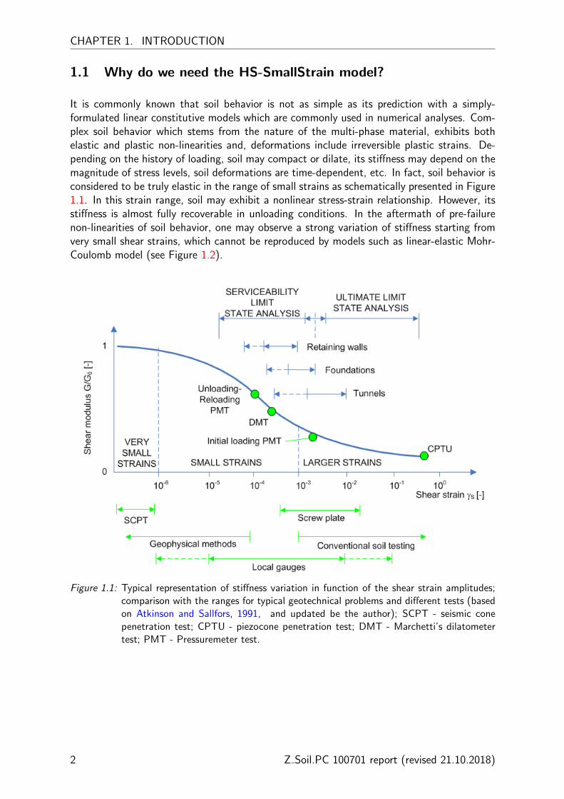
It is commonly known that soil behavior is not as simple as its prediction with a simply-formulated linear constitutive models which are commonly used in numerical analyses. Com-plex soil behavior which stems from the nature of the multi-phase material, exhibits bothelastic and plastic non-linearities and, deformations include irreversible plastic strains. De-pending on the history of loading, soil may compact or dilate, its stiffness may depend on themagnitude of stress levels, soil deformations are time-dependent, etc. In fact, soil behavior isconsidered to be truly elastic in the range of small strains as schematically presented in Figure1.1. In this strain range, soil may exhibit a nonlinear stress-strain relationship. However, itsstiffness is almost fully recoverable in unloading conditions. In the aftermath of pre-failurenon-linearities of soil behavior, one may observe a strong variation of stiffness starting fromvery small shear strains, which cannot be reproduced by models such as linear-elastic Mohr-Coulomb model (see Figure 1.2).
Figure 1.1: Typical representation of stiffness variation in function of the shear strain amplitudes;comparison with the ranges for typical geotechnical problems and different tests (basedon Atkinson and Sallfors, 1991, and updated be the author); SCPT - seismic conepenetration test; CPTU - piezocone penetration test; DMT - Marchetti’s dilatometertest; PMT - Pressuremeter test.
2 Z Soil.PC 100701 report (revised 21.10.2018)
1.1. WHY DO WE NEED THE HS-SMALLSTRAIN MODEL?
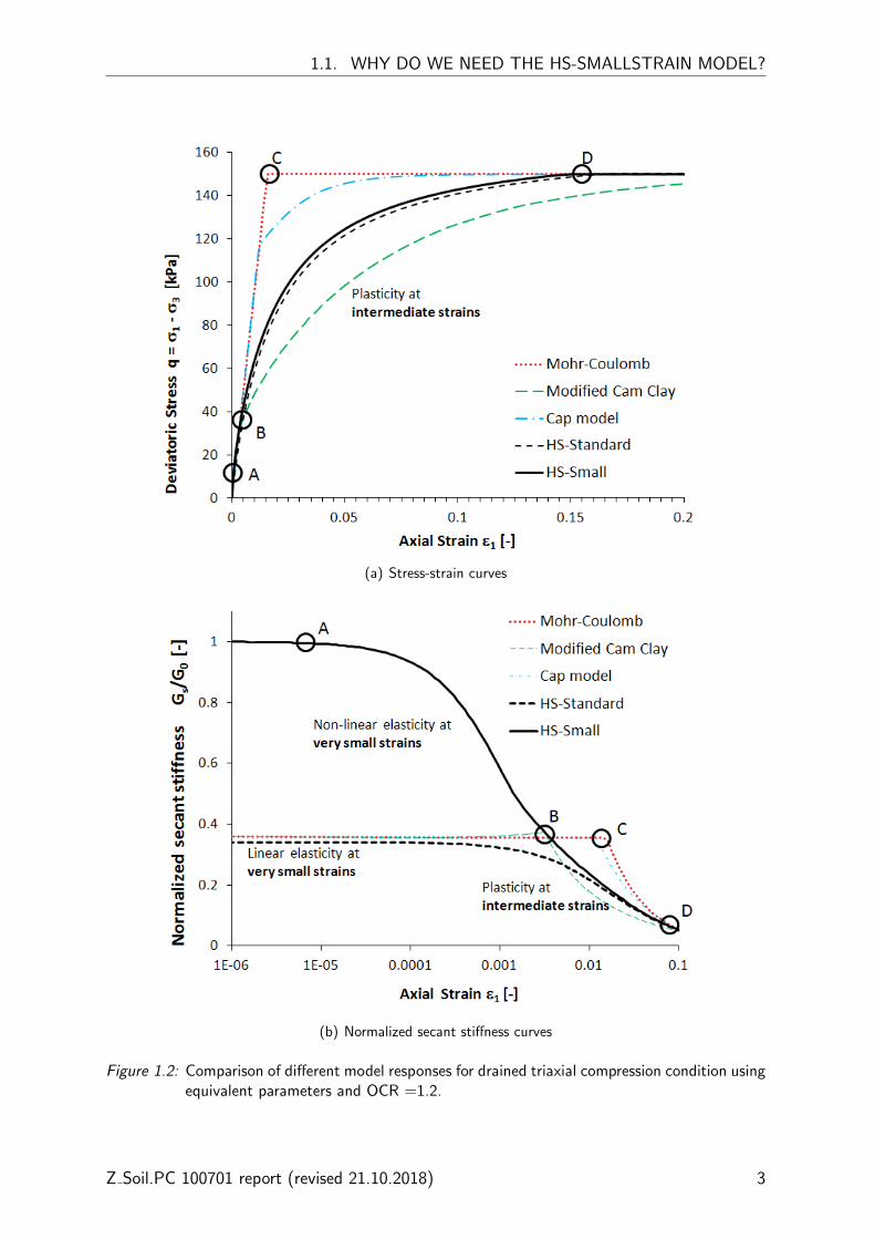
(a) Stress-strain curves
(b) Normalized secant stiffness curves
Figure 1.2: Comparison of different model responses for drained triaxial compression condition usingequivalent parameters and OCR =1.2.
Z Soil.PC 100701 report (revised 21.10.2018) 3
CHAPTER 1. INTRODUCTION
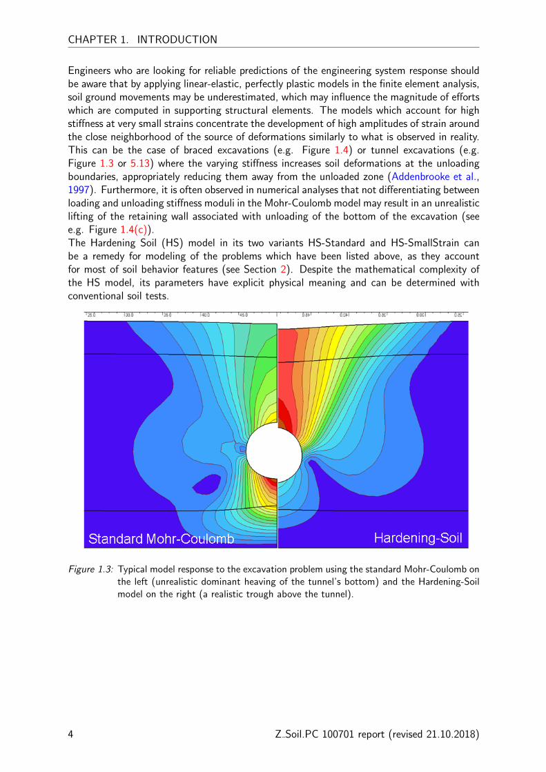
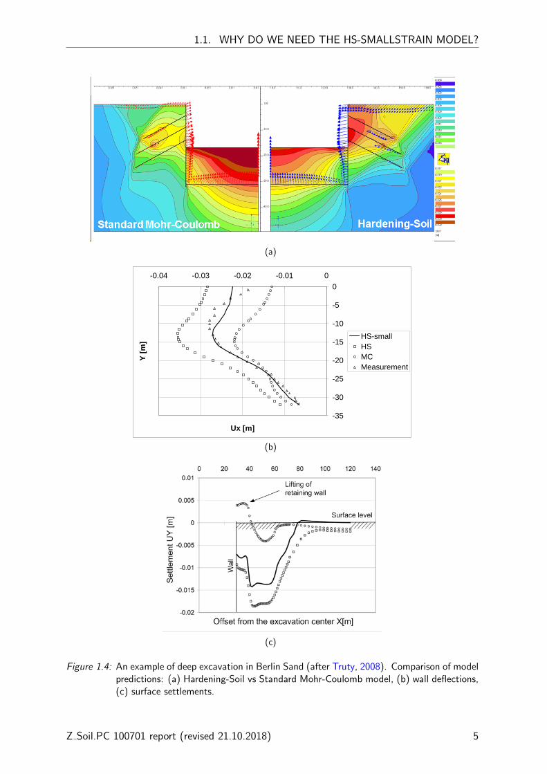
Engineers who are looking for reliable predictions of the engineering system response shouldbe aware that by applying linear-elastic, perfectly plastic models in the finite element analysis,soil ground movements may be underestimated, which may influence the magnitude of effortswhich are computed in supporting structural elements. The models which account for highstiffness at very small strains concentrate the development of high amplitudes of strain aroundthe close neighborhood of the source of deformations similarly to what is observed in reality.This can be the case of braced excavations (e.g. Figure 1.4) or tunnel excavations (e.g.Figure 1.3 or 5.13) where the varying stiffness increases soil deformations at the unloadingboundaries, appropriately reducing them away from the unloaded zone (Addenbrooke et al.,1997). Furthermore, it is often observed in numerical analyses that not differentiating betweenloading and unloading stiffness moduli in the Mohr-Coulomb model may result in an unrealisticlifting of the retaining wall associated with unloading of the bottom of the excavation (seee.g. Figure 1.4(c)).The Hardening Soil (HS) model in its two variants HS-Standard and HS-SmallStrain canbe a remedy for modeling of the problems which have been listed above, as they accountfor most of soil behavior features (see Section 2). Despite the mathematical complexity ofthe HS model, its parameters have explicit physical meaning and can be determined withconventional soil tests.
Figure 1.3: Typical model response to the excavation problem using the standard Mohr-Coulomb onthe left (unrealistic dominant heaving of the tunnel’s bottom) and the Hardening-Soilmodel on the right (a realistic trough above the tunnel).
4 Z Soil.PC 100701 report (revised 21.10.2018)
1.1. WHY DO WE NEED THE HS-SMALLSTRAIN MODEL?
(a)
-35
-30
-25
-20
-15
-10
-5
0-0.04 -0.03 -0.02 -0.01 0
Ux [m]
Y [m
] HS-smallHSMCMeasurement
(b)
(c)
Figure 1.4: An example of deep excavation in Berlin Sand (after Truty, 2008). Comparison of modelpredictions: (a) Hardening-Soil vs Standard Mohr-Coulomb model, (b) wall deflections,(c) surface settlements.
Z Soil.PC 100701 report (revised 21.10.2018) 5
CHAPTER 1. INTRODUCTION
SANDS CLAYS
Degree ofOverconsolidation
Normal,Soft clays
SILTS
Dilatant,Low
compressible
Non-dilatant,Compressible
Selectedsoil models
implemented in Z_Soil
Mohr-Coulomb (Drucker-Prager)
CAP
Modified Cam-Clay
HS-StandardHS-Small Strain
HS-Small Strain HS-Std
HighStiff clays
Low
Type ofanalysis
SLSULS
SLSULS
SLSULS
SLS
ULS
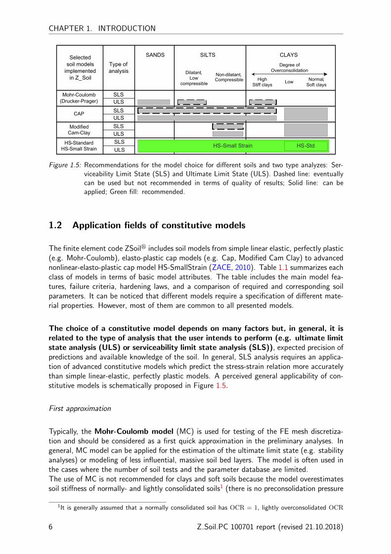
Figure 1.5: Recommendations for the model choice for different soils and two type analyzes: Ser-viceability Limit State (SLS) and Ultimate Limit State (ULS). Dashed line: eventuallycan be used but not recommended in terms of quality of results; Solid line: can beapplied; Green fill: recommended.
1.2 Application fields of constitutive models
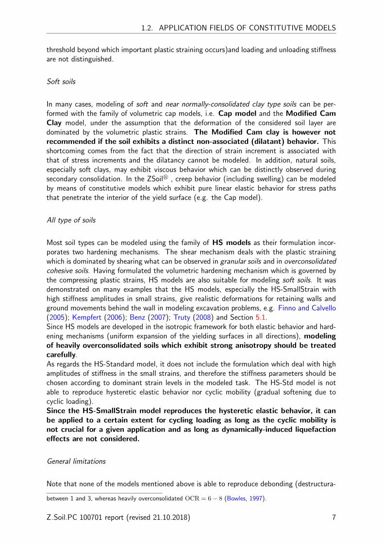
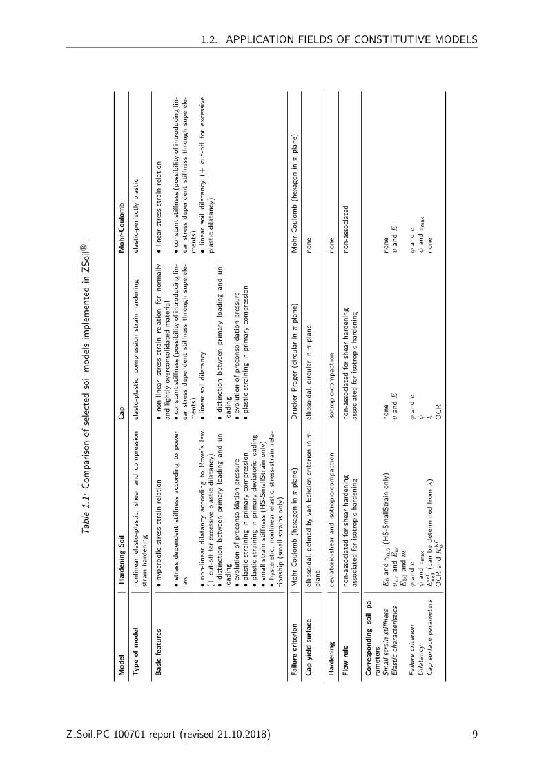
The finite element code ZSoilr includes soil models from simple linear elastic, perfectly plastic(e.g. Mohr-Coulomb), elasto-plastic cap models (e.g. Cap, Modified Cam Clay) to advancednonlinear-elasto-plastic cap model HS-SmallStrain (ZACE, 2010). Table 1.1 summarizes eachclass of models in terms of basic model attributes. The table includes the main model fea-tures, failure criteria, hardening laws, and a comparison of required and corresponding soilparameters. It can be noticed that different models require a specification of different mate-rial properties. However, most of them are common to all presented models.
The choice of a constitutive model depends on many factors but, in general, it isrelated to the type of analysis that the user intends to perform (e.g. ultimate limitstate analysis (ULS) or serviceability limit state analysis (SLS)), expected precision ofpredictions and available knowledge of the soil. In general, SLS analysis requires an applica-tion of advanced constitutive models which predict the stress-strain relation more accuratelythan simple linear-elastic, perfectly plastic models. A perceived general applicability of con-stitutive models is schematically proposed in Figure 1.5.
First approximation
Typically, the Mohr-Coulomb model (MC) is used for testing of the FE mesh discretiza-tion and should be considered as a first quick approximation in the preliminary analyses. Ingeneral, MC model can be applied for the estimation of the ultimate limit state (e.g. stabilityanalyses) or modeling of less influential, massive soil bed layers. The model is often used inthe cases where the number of soil tests and the parameter database are limited.The use of MC is not recommended for clays and soft soils because the model overestimatessoil stiffness of normally- and lightly consolidated soils1 (there is no preconsolidation pressure
1It is generally assumed that a normally consolidated soil has OCR = 1, lightly overconsolidated OCR
6 Z Soil.PC 100701 report (revised 21.10.2018)
1.2. APPLICATION FIELDS OF CONSTITUTIVE MODELS
threshold beyond which important plastic straining occurs)and loading and unloading stiffnessare not distinguished.
Soft soils
In many cases, modeling of soft and near normally-consolidated clay type soils can be per-formed with the family of volumetric cap models, i.e. Cap model and the Modified CamClay model, under the assumption that the deformation of the considered soil layer aredominated by the volumetric plastic strains. The Modified Cam clay is however notrecommended if the soil exhibits a distinct non-associated (dilatant) behavior. Thisshortcoming comes from the fact that the direction of strain increment is associated withthat of stress increments and the dilatancy cannot be modeled. In addition, natural soils,especially soft clays, may exhibit viscous behavior which can be distinctly observed duringsecondary consolidation. In the ZSoilr , creep behavior (including swelling) can be modeledby means of constitutive models which exhibit pure linear elastic behavior for stress pathsthat penetrate the interior of the yield surface (e.g. the Cap model).
All type of soils
Most soil types can be modeled using the family of HS models as their formulation incor-porates two hardening mechanisms. The shear mechanism deals with the plastic strainingwhich is dominated by shearing what can be observed in granular soils and in overconsolidatedcohesive soils. Having formulated the volumetric hardening mechanism which is governed bythe compressing plastic strains, HS models are also suitable for modeling soft soils. It wasdemonstrated on many examples that the HS models, especially the HS-SmallStrain withhigh stiffness amplitudes in small strains, give realistic deformations for retaining walls andground movements behind the wall in modeling excavation problems, e.g. Finno and Calvello(2005); Kempfert (2006); Benz (2007); Truty (2008) and Section 5.1.Since HS models are developed in the isotropic framework for both elastic behavior and hard-ening mechanisms (uniform expansion of the yielding surfaces in all directions), modelingof heavily overconsolidated soils which exhibit strong anisotropy should be treatedcarefully.As regards the HS-Standard model, it does not include the formulation which deal with highamplitudes of stiffness in the small strains, and therefore the stiffness parameters should bechosen according to dominant strain levels in the modeled task. The HS-Std model is notable to reproduce hysteretic elastic behavior nor cyclic mobility (gradual softening due tocyclic loading).Since the HS-SmallStrain model reproduces the hysteretic elastic behavior, it canbe applied to a certain extent for cycling loading as long as the cyclic mobility isnot crucial for a given application and as long as dynamically-induced liquefactioneffects are not considered.
General limitations
Note that none of the models mentioned above is able to reproduce debonding (destructura-
between 1 and 3, whereas heavily overconsolidated OCR = 6− 8 (Bowles, 1997).
Z Soil.PC 100701 report (revised 21.10.2018) 7

CHAPTER 1. INTRODUCTION
tion) effects which can be observed as softening in the sensitive soils. It should also be notedthat the cap hardening parameter (preconsolidation pressure) is not coupled with the degreeof saturation, and therefore modeling of collapsible behavior of partially saturated soils is notpossible with the implemented models.
8 Z Soil.PC 100701 report (revised 21.10.2018)
1.2. APPLICATION FIELDS OF CONSTITUTIVE MODELS
Tab
le1.
1:C
omp
aris
onof
sele
cted
soil
mo
del
sim
ple
men
ted
inZ
Soi
lr.
Mo
del
Har
den
ing
So
ilC
ap
Mo
hr-
Co
ulo
mb
Typ
eo
fm
od
eln
on
lin
ear
ela
sto
-pla
stic
,sh
ear
an
dco
mp
ress
ion
stra
inh
ard
enin
gel
ast
o-p
last
ic,
com
pre
ssio
nst
rain
har
den
ing
ela
stic
-per
fect
lyp
last
ic
Ba
sic
fea
ture
s•
hyp
erb
olic
stre
ss-s
tra
inre
lati
on
•n
on
-lin
ear
stre
ss-s
tra
inre
lati
on
for
nor
ma
lly
an
dlig
htl
yo
verc
on
solid
ate
dm
ate
ria
l•
lin
ear
stre
ss-s
tra
inre
lati
on
•st
ress
dep
end
ent
stiff
nes
sa
ccor
din
gto
pow
erla
w•
con
sta
nt
stiff
nes
s(p
oss
ibilit
yo
fin
tro
du
cin
glin
-ea
rst
ress
dep
end
ent
stiff
nes
sth
rou
gh
sup
erel
e-m
ents
)
•co
nst
an
tst
iffn
ess
(po
ssib
ilit
yo
fin
tro
du
cin
glin
-ea
rst
ress
dep
end
ent
stiff
nes
sth
rou
gh
sup
erel
e-m
ents
)•
no
n-l
inea
rd
ila
tan
cya
ccor
din
gto
Row
e’s
law
(+cu
t-o
fffo
rex
cess
ive
pla
stic
dila
tan
cy)
•lin
ear
soil
dila
tan
cy•
lin
ear
soil
dila
tan
cy(+
cut-
off
for
exce
ssiv
ep
last
icd
ila
tan
cy)
•d
isti
nct
ion
bet
wee
np
rim
ary
loa
din
ga
nd
un
-lo
ad
ing
•d
isti
nct
ion
bet
wee
np
rim
ary
loa
din
ga
nd
un
-lo
ad
ing
•ev
olu
tio
no
fp
reco
nso
lid
ati
on
pre
ssu
re•
evo
luti
on
of
pre
con
solid
ati
on
pre
ssu
re•
pla
stic
stra
inin
gin
pri
mar
yco
mp
ress
ion
•p
last
icst
rain
ing
inp
rim
ary
com
pre
ssio
n•
pla
stic
stra
inin
gin
pri
mar
yd
evia
tori
clo
ad
ing
•sm
all
stra
inst
iffn
ess
(HS
-Sm
allS
tra
ino
nly
)•
hys
tere
tic,
no
nlin
ear
ela
stic
stre
ss-s
tra
inre
la-
tio
nsh
ip(s
ma
llst
rain
so
nly
)
Fa
ilure
crit
erio
nM
oh
r-C
ou
lom
b(h
exa
go
ninπ
-pla
ne)
Dru
cker
-Pra
ger
(cir
cula
rinπ
-pla
ne)
Mo
hr-
Co
ulo
mb
(hex
ag
on
inπ
-pla
ne)
Ca
pyi
eld
surf
ace
ellip
soid
al,
defi
ned
by
van
Eek
elen
crit
erio
ninπ
-p
lan
eel
lip
soid
al,
circ
ula
rinπ
-pla
ne
no
ne
Har
den
ing
dev
iato
ric-
shea
ra
nd
iso
tro
pic
-co
mp
act
ion
iso
tro
pic
-co
mp
act
ion
no
ne
Flo
wru
len
on
-ass
oci
ate
dfo
rsh
ear
har
den
ing
no
n-a
sso
cia
ted
for
shea
rh
ard
enin
gn
on
-ass
oci
ate
da
sso
cia
ted
for
iso
tro
pic
har
den
ing
ass
oci
ate
dfo
ris
otr
op
ich
ard
enin
g
Co
rres
po
nd
ing
soil
pa
-ra
met
ers
Sm
all
stra
inst
iffn
ess
E0
an
dγ0.7
(HS
-Sm
allS
tra
ino
nly
)n
on
en
on
eE
last
icch
ara
cter
isti
csυur
an
dE
ur
υa
ndE
υa
ndE
E50
an
dm
Fa
ilu
recr
iter
ion
φa
ndc
φa
ndc
φa
ndc
Dila
tan
cyψ
an
de m
ax
ψψ
an
de m
ax
Ca
psu
rfa
cep
ara
met
ers
Ere
fo
ed(c
an
be
det
erm
ined
fro
mλ
)λ
no
ne
OC
Ra
ndK
NC
0O
CR
Z Soil.PC 100701 report (revised 21.10.2018) 9

CHAPTER 1. INTRODUCTION
10 Z Soil.PC 100701 report (revised 21.10.2018)

Chapter 2
Short introduction to the HS models
The Hardening Soil model (HS-Standard) was designed by Schanz (1998); Schanz et al.(1999) in order to reproduce basic macroscopic phenomena exhibited by soils such as:
• densification, i.e. a decrease of voids volume in soil due to plastic deformations, e.g.Figure 2.11;
• stress dependent stiffness, i.e. observed phenomena of increasing stiffness moduli withincreasing stress level (mean stress), e.g. Figure. 2.4;
• soil stress history, i.e. accounting for preconsolidation effects;
• plastic yielding, i.e. development of irreversible strains with reaching a yield criterion,e.g. Figure 2.2;
• dilatation, i.e. an occurrence of negative volumetric strains during shearing, e.g. Figure2.11.
Contrary to other models such us the Cap model or the Modified Cam Clay (let alone theMohr-Coulmb model), the magnitude of soil deformations can be modeled more accurately byincorporating three input stiffness parameters corresponding to the triaxial loading stiffness(E50), the triaxial unloading-reloading stiffness (Eur), and the oedometer loading modulus(Eoed).
An enhanced version of the HS-Standard, the Hardening Soil Small model (HS-SmallStrain)was formulated by Benz (2007) in order to handle a commonly observed phenomena of:
• strong stiffness variation with increasing shear strain amplitudes in the domain of smallstrains (Figure 1.1);
• hysteretic, nonlinear elastic stress-strain relationship which is applicable in the range ofsmall strains (Figure 2.20).
These features mean that the HS-SmallStrain is able to produce more accurate and reliableapproximation of displacements which can be useful for dynamic applications or in modelingunloading-conditioned problems, e.g. deep excavations with retaining walls.

CHAPTER 2. SHORT INTRODUCTION TO THE HS MODELS
Figure 2.1: Schematic presentation of the Hardening-Soil model framework vis-a-vis the degradationof shear stiffness with increasing shear strains.
Although both models can be considered as advanced soil models which are able to faithfullyapproximate complex soil behavior, they include some limitations related to specific behaviorobserved for certain soils. The models are not able to reproduce softening effects associatedwith soil dilatancy and soil destructuration (debonding of cemented particles) which can beobserved, for instance, in sensitive soils. As opposed to the HS-SmallStrain model, the HS-Standard does not account for large amplitudes of soil stiffness related to transition fromvery small strain to engineering strain levels (ε ≈ 10−3 − 10−2). Therefore, the user shouldadapt the stiffness characteristics to the strain levels which are expected to take place inconditions of the analyzed problem. Moreover, the HS-Standard model is not capable toreproduce hysteretic soil behavior observed during cycling loading.As an enhanced version of the HS-Standard model, HS-SmallStrain accounts for smallstrain stiffness and therefore, it can be used to some extent to model hysteretic soil behaviorunder cyclic loading conditions with the exception of gradual softening which is experimentallyobserved with an increasing number of loading cycles.
12 Z Soil.PC 100701 report (revised 21.10.2018)

2.1. HARDENING SOIL-STANDARD MODEL
2.1 Hardening Soil-Standard model
2.1.1 Shear mechanism
The shear mechanism is introduced in order to handle the soil hardening which is inducedby the plastic shear strains. Domination of plastic shear strains can be typically observed forgranular materials such as sands, and heavily consolidated cohesive soils.
2.1.1.1 Shear yield mechanism
The hardening yield function for shear mechanism f1, is described using the concept ofhyperbolic approximation of the relation between the vertical strain ε1 and deviatoric stressq for a standard triaxial drained compression test (Figure 2.2). The yield condition is thusexpressed as follows:
Figure 2.2: Hyperbolic stress-strain relationship and the definition of different moduli in the triaxialdrained test condition.
f1 =qaE50
q
qa − q− 2
q
Eur− γPS for q < qf (2.1)
where γPS is the plastic strain hardening parameter, qa is the asymptotic deviatoric stresswhich is defined by the ultimate deviatoric stress qf and the failure ratio 1 Rf is defines as:
qa =qfRf
(2.2)
1A suitable value of the failure ratio is set by default Rf = 0.9. For most soils, the value of Rf fallsbetween 0.75 and 1. See also Section 3.3.3.
Z Soil.PC 100701 report (revised 21.10.2018) 13
CHAPTER 2. SHORT INTRODUCTION TO THE HS MODELS
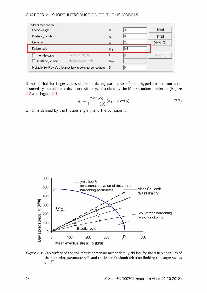
It means that for larger values of the hardening parameter γPS, the hyperbolic relation is re-strained by the ultimate deviatoric stress qf described by the Mohr-Coulomb criterion (Figure2.2 and Figure 2.3):
qf =2 sin(φ)
1− sin(φ)(σ3 + c cotφ) (2.3)
which is defined by the friction angle φ and the cohesion c.
Figure 2.3: Cap surface of the volumetric hardening mechanism, yield loci for the different values ofthe hardening parameter γPS and the Mohr-Coulomb criterion limiting the larger valuesof γPS.
14 Z Soil.PC 100701 report (revised 21.10.2018)
2.1. HARDENING SOIL-STANDARD MODEL
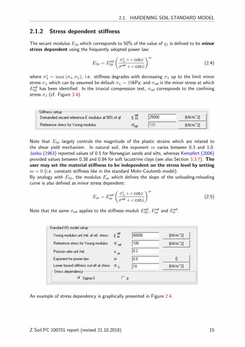
2.1.2 Stress dependent stiffness
The secant modulus E50 which corresponds to 50% of the value of qf is defined to be minorstress dependent using the frequently adopted power law:
E50 = Eref50
(σ∗3 + c cotφ
σref + c cotφ
)m(2.4)
where σ∗3 = max (σ3, σL), i.e. stiffness degrades with decreasing σ3 up to the limit minorstress σL which can by assumed be default σL = 10kPa; and σref is the minor stress at whichEref
50 has been identified. In the triaxial compression test, σref corresponds to the confiningstress σ3 (cf. Figure 3.4).
Note that E50 largely controls the magnitude of the plastic strains which are related tothe shear yield mechanism. In natural soil, the exponent m varies between 0.3 and 1.0.Janbu (1963) reported values of 0.5 for Norwegian sands and silts, whereas Kempfert (2006)provided values between 0.38 and 0.84 for soft lacustrine clays (see also Section 3.3.7). Theuser may set the material stiffness to be independent on the stress level by settingm = 0 (i.e. constant stiffness like in the standard Mohr-Coulomb model).By analogy with E50, the modulus Eur which defines the slope of the unloading-reloadingcurve is also defined as minor stress dependent:
Eur = Erefur
(σ∗3 + c cotφ
σref + c cotφ
)m(2.5)
Note that the same σref applies to the stiffness moduli Eref50 , Eref
ur and Eref0 .
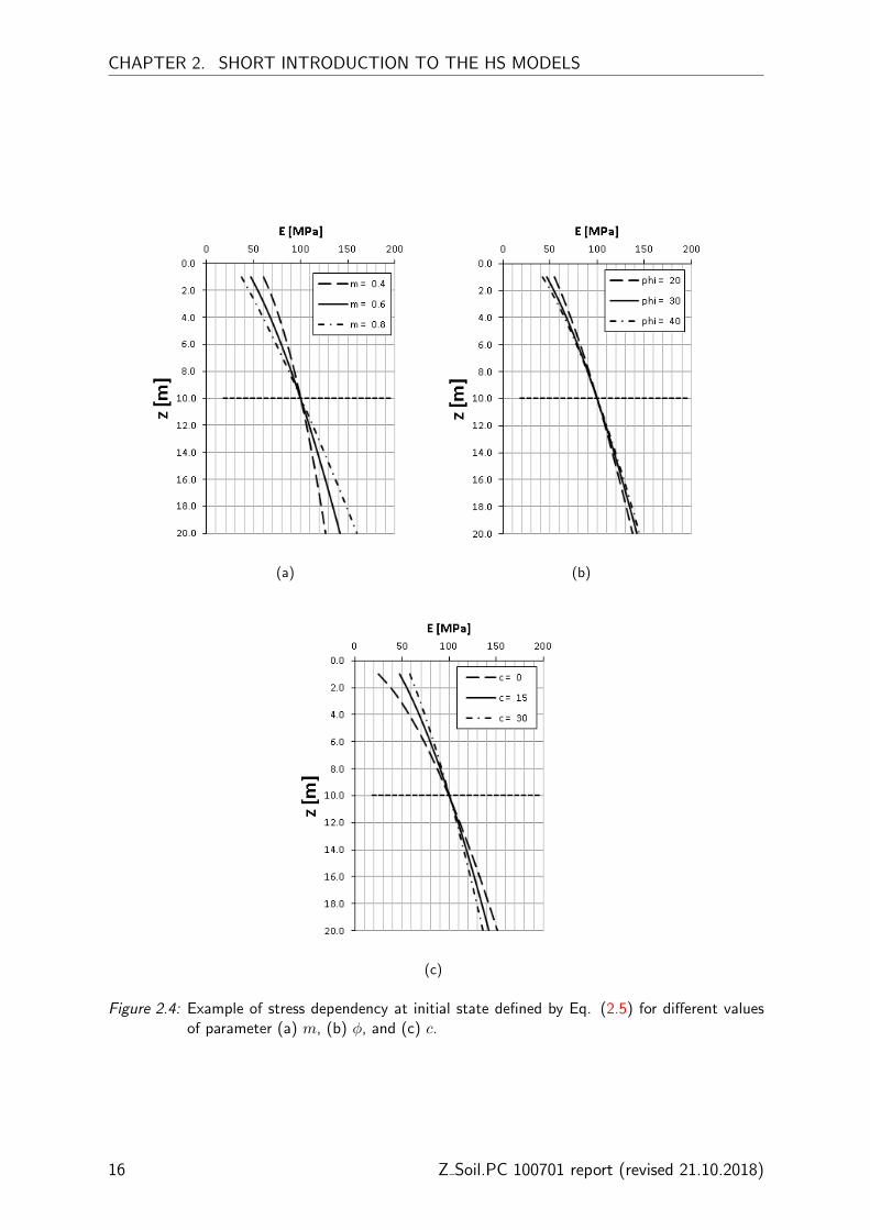
An example of stress dependency is graphically presented in Figure 2.4.
Z Soil.PC 100701 report (revised 21.10.2018) 15
CHAPTER 2. SHORT INTRODUCTION TO THE HS MODELS
(a) (b)
(c)
Figure 2.4: Example of stress dependency at initial state defined by Eq. (2.5) for different valuesof parameter (a) m, (b) φ, and (c) c.
16 Z Soil.PC 100701 report (revised 21.10.2018)

2.1. HARDENING SOIL-STANDARD MODEL
2.1.2.1 Stress dependent stiffness based on the mean effective stress.
It can observed that in the case of dynamic analyzes or modeling of excavation problem withoverconsolidation soils which exhibit K0 > 1, a rotation of principal stress may occur resultingin spurious oscillations of stiffness moduli. For example, in the case of excavation of a circulartunnel, one may observe the rotation of principal stresses at the tunnel sides, and the verticalstress which initially defines the soil stiffness σ3 = σ′v becomes σ3 = σ′h which may leadto an underestimation of soil stiffness. This is because σ′h decreases to zero dropping theunloading-reloading stiffness to its minimal value which is limited by σL. Moreover, at thebottom of an excavated tunnel σ3 which is equal to the vertical stress may also drop to zeroresulting in slightly overestimated swelling of the tunnel bottom.In order to remedy this problem, the user can use the stress dependency formulation which
depend on the mean effective stress p′ which can be written in a general form as:
E = Eref
(p∗
σref
)mp
with p∗ = max(p′, σL) (2.6)
where:σref - reference stressEref - reference modulus corresponding to the reference stress σref
mp - stiffness exponent for p′-formulation which is equal to mp = m if c = 0,otherwise mp 6= m
p′ - mean effective stress (σ′1 + σ′2 + σ′3)/3σL - the limiting stress (in order to avoid zero stiffness when p′ is close to 0)
A unique σref applies to the stiffness moduli Eref50 , Eref
ur and Eref0 .
In the current version (ZSoil v2018 ), the evolution of the preconsolidation parameter (refer toEq. 2.23) remains the same for both formulations of stiffness dependency and it contains thecomponent c cotφ. Note that parameter transformation does not apply to Eref
oed because thisinput parameter is not a model parameter but it serves as the reference value for calibratingparameters M and H.
Table 2.1: Comparison of two approaches which describe stress dependent stiffness.
Minor effective stress σ′3 Mean effective stress p′
Drawback: Spurious oscillations of stiffnessmoduli in the case of dynamic analyzes and ex-cavation problems in materials with K0 > 1
Stiffness oscillations independent of the principalstresses rotation
Drawback: Underestimation of unloading-reloading stiffness in excavation problems
Unloading-reloading stiffness depends on p′
which is larger than σ3 in excavation problems
Direct identification of the stiffness moduli E50
and Eur for the constant σ3 during triaxial com-pression test
Drawback: E50 and Eur are not directly iden-tifiable from triaxial test as p′ varies during tri-axial compression test. A simple transformationmethod is provided in Figure 2.5.
Z Soil.PC 100701 report (revised 21.10.2018) 17

CHAPTER 2. SHORT INTRODUCTION TO THE HS MODELS
In ZSoil v2018 , p-stress dependency can be activated in Elastic dialog window ( X Advancedoption has to be checked), as illustrated below.
2.1.2.2 Parameter migration between minor and mean stress for-mulations
Note that the initial material stiffness described by σ3-formulation and p′-formulation may bedifferent across the soil profile for the same σref if the same reference moduli Eσ,ref
0 (σref) =Ep,ref
0 (σref) and the same stiffness exponent m = mp are taken. In the other words, assumingthe same departing stiffness profile for both formulations one should be aware that:
• the reference moduli are different Eσ3,ref0 (σref) 6= Ep,ref
0 (σref) if K0 6= 1
• the stiffness exponents m and mp are different if c > 0
In order to preserve the same or similar variation of E0 across the soil profile obtained forσ3-formulation, one may adjust Ep.ref
0 to the same value of σref by proceeding the followingprocedure:
1. Determine Eref, m for a given σref, φ′ and, c′ assuming σ3-formulation
e.g. for σref = 100kPa, the following parameters were obtained from triaxial compression tests: Eur =
260000kPa, m = 0.5, φ′ = 30o and c = 5kPa
2. Specify n-number of different effective vertical stresses σ′v0 and in situ stress ratio K0 (inorder to determine σ3)
18 Z Soil.PC 100701 report (revised 21.10.2018)
2.1. HARDENING SOIL-STANDARD MODEL
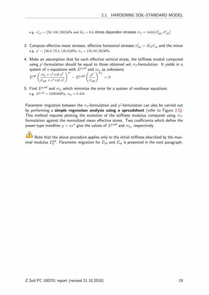
e.g. σ′v0 = {50, 100, 200}kPa and K0 = 0.6 stress dependen stresses σ3 = min(σ′h0, σ′v0)
3. Compute effective mean stresses, effective horizontal stresses σ′h0 = K0σ′v0 and the minor
e.g. p′ = {36.6, 73.3, 146.6}kPa, σ3 = {30, 60, 90}kPa
4. Make an assumption that for each effective vertical stress, the stiffness moduli computedusing p′-formulation should be equal to those obtained wit σ3-formulation. It yields in asystem of n-equations with Ep,ref and mp as unknowns:
Eref
(σ3 + c′ cotφ′
σref + c′ cotφ′
)m− Ep,ref
(p′
σref
)mp
= 0
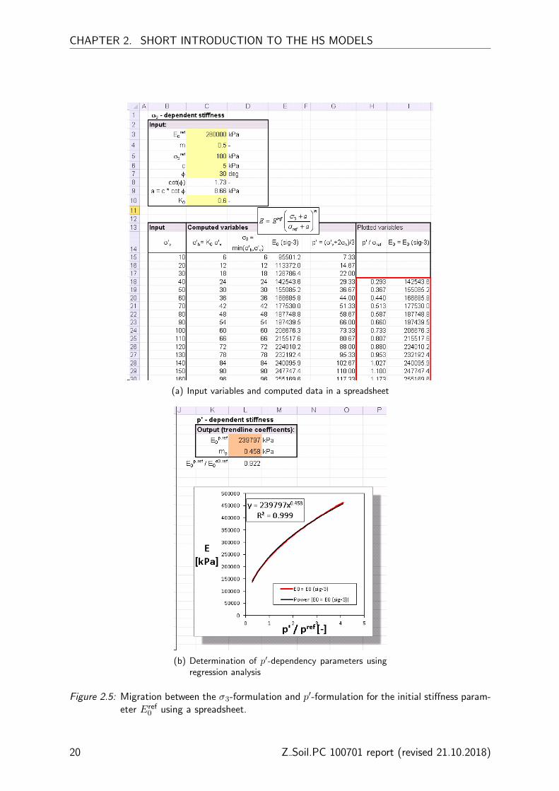
5. Find Ep,ref and mp which minimize the error for a system of nonlinear equations.e.g. Ep,ref = 229938kPa, mp = 0.458
Parameter migration between the σ3-formulation and p′-formulation can also be carried outby performing a simple regression analysis using a spreadsheet (refer to Figure 2.5).This method requires plotting the evolution of the stiffness modulus computed using σ3-formulation against the normalized mean effective stress. Two coefficients which define thepower-type trendline y = axb give the values of Ep,ref and mp, respectively.
Note that the above procedure applies only to the initial stiffness described by the max-imal modulus Eref
0 . Parameter migration for E50 and Eur is presented in the next paragraph.
Z Soil.PC 100701 report (revised 21.10.2018) 19
CHAPTER 2. SHORT INTRODUCTION TO THE HS MODELS
(a) Input variables and computed data in a spreadsheet
(b) Determination of p′-dependency parameters usingregression analysis
Figure 2.5: Migration between the σ3-formulation and p′-formulation for the initial stiffness param-eter Eref
0 using a spreadsheet.
20 Z Soil.PC 100701 report (revised 21.10.2018)
2.1. HARDENING SOIL-STANDARD MODEL
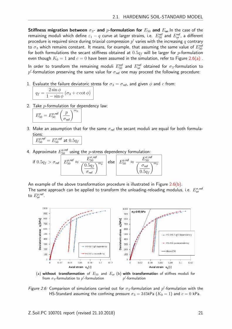
Stiffness migration between σ3- and p-formulation for E50 and Eur.In the case of theremaining moduli which define ε1 − q curve at larger strains, i.e. Eref
50 and Erefur , a different
procedure is required since during triaxial compression p′ varies with the increasing q contraryto σ3 which remains constant. It means, for example, that assuming the same value of Eref
50
for both formulations the secant stiffness obtained at 0.5qf will be larger for p-formulationeven though K0 = 1 and c = 0 have been assumed in the simulation, refer to Figure 2.6(a) .
In order to transform the remaining moduli Eref50 and Eref
ur obtained for σ3-formulation top′-formulation preserving the same value for σref one may proceed the following procedure:
1. Evaluate the failure deviatoric stress for σ3 = σref, and given φ and c from:
qf =2 sinφ
1− sinφ(σ3 + c cotφ)
2. Take p-formulation for dependency law:
Ep50 = Ep,ref
50
(p
σref
)mp
3. Make an assumption that for the same σref the secant moduli are equal for both formula-tions:
Ep,ref50 = Eσ,ref
50 at 0.5qf
4. Approximate Ep,ref50 using the p-stress dependency formulation:
if 0.5qf > σref Ep,ref50 ≈ Eσ,ref
50(0.5qfσref
)mpelse Ep,ref
50 ≈ Eσ,ref50(
σref
0.5qf
)mp
An example of the above transformation procedure is illustrated in Figure 2.6(b).The same approach can be applied to transform the unloading-reloading modulus, i.e. Eσ,ref
ur
to Ep,refur .
(a) without transformation of E50 and Eur
from σ3-formulation to p′-formulation(b) with transformation of stiffnes moduli for
p′-formulation
Figure 2.6: Comparison of simulations carried out for σ3-formulation and p′-formulation with theHS-Standard assuming the confining pressure σ3 = 345kPa (K0 = 1) and c = 0 kPa.
Z Soil.PC 100701 report (revised 21.10.2018) 21

CHAPTER 2. SHORT INTRODUCTION TO THE HS MODELS
2.1.2.2.1 Integrated tool for moduli migration
Virtual Lab v2018 offers and an integrated toolbox for moduli migration (Figure 2.7). Thetool includes the migration approaches which are presented above.
Figure 2.7: Parameter migration between the two formulations for stress dependent stiffness inVirtual Lab v2018 .
22 Z Soil.PC 100701 report (revised 21.10.2018)

2.1. HARDENING SOIL-STANDARD MODEL
2.1.3 Shear hardening law
The shear hardening yield function f1 can be decomposed into part which is a function ofstress - two first components, whereas the last component is a function of plastic strainsγPS = εp1− ε
p2− ε
p3. Assuming that in the contractancy domain, the volumetric plastic strain
εpv = εp1 + εp2 + εp3 is observed to be very small εpv ≈ 0, it can thus be written:
γPS ∼= 2εp1 (2.7)
Hence, for the primary loading in drained triaxial conditions, ε1 is evaluated using the yieldcondition f1 (Eq.(2.1)) and decomposition of the elastic and the plastic strains:
ε1 = εe1 + εp1 =q
Eur+
1
2
(qaE50
q
qa − q− 2q
Eur
)=
qa2E50
q
qa − q(2.8)
For the drained triaxial conditions and the confining stress remaining constant (i.e. σ2 =σ3 = const.), the modulus Eur remains constant and the elastic strains can be computedfrom:
εe1 =q
Eurand εe2 = εe3 = νur
q
Eur(2.9)
where νur denotes unloading/reloading Poisson’s ratio.
The hyperbolic relation between the axial strain and the deviatoric stress presented in Equation2.8 can be rearranged into:
q =ε1
1
2E50
+ε1Rf
qf
(2.10)
which can also be rewritten in the following form:
q =ε1
a+ bε1(2.11)
These equations are graphically presented in Figure 2.8.Note that for an anisotropically consolidated clay, the initial state deviatoric stress (afterconsolidation but before compression) which corresponds to the state of zero strains is:
q0 = σ31−K0
K0
(2.12)
so the the deviatoric stress after consolidation becomes:
qm = q − q0 (2.13)
and Eq.(2.10) can be rewritten as:
qm =ε1
1
2E50
+ε1Rf
qm,f
(2.14)
with qm,f denoting qm at failure.
Z Soil.PC 100701 report (revised 21.10.2018) 23

CHAPTER 2. SHORT INTRODUCTION TO THE HS MODELS
(a) (b)
Figure 2.8: Graphical representation of Eq.(2.10) and identification of failure ratio Rf (a) hyperboliccurve plotted with laboratory data points (b) typical triaxial drained compression resultspresented in the hyperbolic form (laboratory data from Kempfert, 2006).
2.1.4 Plastic flow rule and dilatancy
The plastic flow rule is derived from the plastic potential:
g1 =σ1 − σ3
2+σ1 + σ3
2sinψm (2.15)
and it takes the linear form:εpv = γp sinψm (2.16)
where the mobilized dilatancy angle ψm is calculated in the HS-Standard model accordingto:
sinψm = 0 if φm < φcs (cut-off in contractancy domain) (2.17a)
sinψm =sinφm − sinφcs
1− sinφm sinφcsif φm ≥ φcs (Rowe’s dilatancy) (2.17b)
where the mobilized friction angle2, φm, is computed from:
sinφm =σ1 − σ3
σ1 + σ3 − 2c cotφ(2.18)
and the critical state friction angle which is a material property and is independent of thestress conditions, is defined by the friction angle φ and the ultimate dilatancy angle ψ as:
sinφcs =sinφ− sinψ
1− sinφ sinψ(2.19)
It means that dilatancy may occur for the larger values of the mobilized friction angle φm >φcs, whereas for smaller stress ratios (φm < φcs), the material contracts and the mobilized
2The mobilized friction angle φm describes the stress ratio τ/σ (at the critical state φm = φcs).
24 Z Soil.PC 100701 report (revised 21.10.2018)
2.1. HARDENING SOIL-STANDARD MODEL
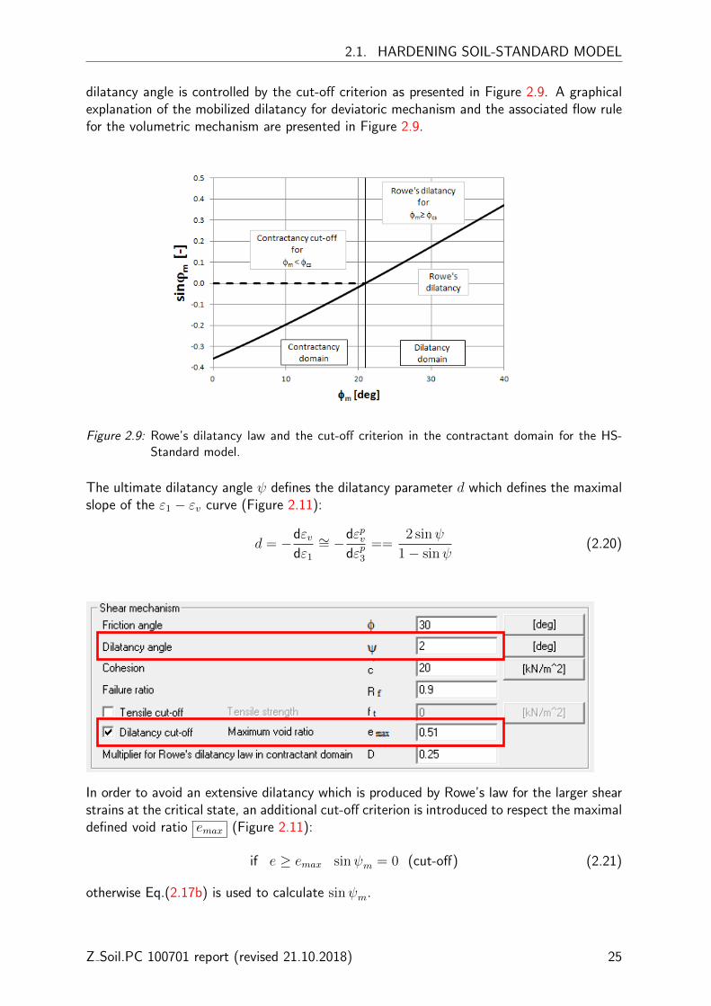
dilatancy angle is controlled by the cut-off criterion as presented in Figure 2.9. A graphicalexplanation of the mobilized dilatancy for deviatoric mechanism and the associated flow rulefor the volumetric mechanism are presented in Figure 2.9.
Figure 2.9: Rowe’s dilatancy law and the cut-off criterion in the contractant domain for the HS-Standard model.
The ultimate dilatancy angle ψ defines the dilatancy parameter d which defines the maximalslope of the ε1 − εv curve (Figure 2.11):
d = −dεvdε1∼= −
dεpvdεp3
==2 sinψ
1− sinψ(2.20)
In order to avoid an extensive dilatancy which is produced by Rowe’s law for the larger shearstrains at the critical state, an additional cut-off criterion is introduced to respect the maximaldefined void ratio emax (Figure 2.11):
if e ≥ emax sinψm = 0 (cut-off) (2.21)
otherwise Eq.(2.17b) is used to calculate sinψm.
Z Soil.PC 100701 report (revised 21.10.2018) 25

CHAPTER 2. SHORT INTRODUCTION TO THE HS MODELS
(a) Non-associated flow for deviatoric mechanism (b) Associated flow for volumetric mechanism
Figure 2.10: Plastic flow rules in the HS model (a) graphical explanation of mobilized dilatancy ψmwhich increases from 0 up to the input dilatancy angle ψ once M-C line is reached,(b) contractancy increases with compressive p′ stress from zero to maximum value atM-C failure only when cap is mobilized.
εv − εv0 = − ln1 + emax
1 + e0
Figure 2.11: Strain curve for a standard triaxial drained compression test with the dilatancy cut-off.
26 Z Soil.PC 100701 report (revised 21.10.2018)

2.1. HARDENING SOIL-STANDARD MODEL
2.1.5 Volumetric mechanism
The volumetric plastic mechanism is introduced to account for a threshold point beyond(preconsolidation pressure) which important plastic straining occur characterizing a normally-consolidated state of soil. Since the shear mechanism generates no volumetric plastic strainin the contractant domain, the model without volumetric mechanism could significantly over-estimate soil stiffness in virgin compression conditions particularly for normally- and lightlyoverconsolidated cohesive soils. Such a problem can be observed when using, for instance,the Mohr-Coulomb model.
The second yield mechanism is proposed in the form of the cap surface similarly to otherhardening models available in ZSoilr , e.g. Modified Cam Clay or Cap. The yield functionwhich is graphically presented in Figure 2.12 and 2.3, is thus defined as:
f2 =q2
M2r2(θ)+ p′2 + p2c (2.22)
where r(θ) obeys van Eekelen’s formula in order to assure a smooth and convex yield surface(cf. also the formulation of the Modified Cam Clay model); M is the model parameter whichdefines the shape of the cap surface and is related to KNC
0 , and pc denotes the preconsolidationpressure which defines an intersection of the cap surface with the hydrostatic axis p′.
Figure 2.12: 3D representation of strength anisotropy in the HS model with the Mohr-Coulombfailure surface and the cap surface which obeys van Eekelen’s formula.
Evolution of the hardening parameter pc is described by the hardening law:
dpc = −H(pc + c cotφ
σref + c cotφ
)mdεpv (2.23)
where H is the parameter which controls the rate of volumetric plastic strains and is relatedto the tangent oedometric modulus Eoed at given reference oedometric (vertical) stress level(see Figure 3.7(a)).
Z Soil.PC 100701 report (revised 21.10.2018) 27
CHAPTER 2. SHORT INTRODUCTION TO THE HS MODELS
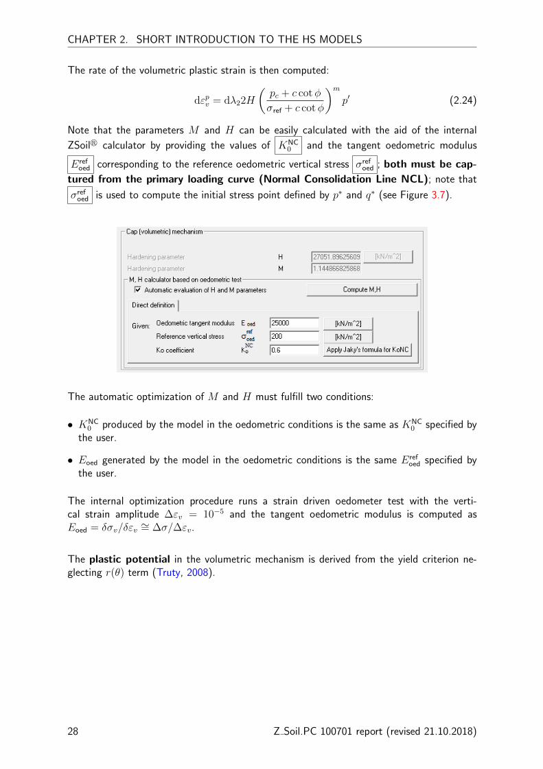
The rate of the volumetric plastic strain is then computed:
dεpv = dλ22H
(pc + c cotφ
σref + c cotφ
)mp′ (2.24)
Note that the parameters M and H can be easily calculated with the aid of the internal
ZSoilr calculator by providing the values of KNC0 and the tangent oedometric modulus
Erefoed corresponding to the reference oedometric vertical stress σref
oed ; both must be cap-
tured from the primary loading curve (Normal Consolidation Line NCL); note that
σrefoed is used to compute the initial stress point defined by p∗ and q∗ (see Figure 3.7).
The automatic optimization of M and H must fulfill two conditions:
• KNC0 produced by the model in the oedometric conditions is the same as KNC
0 specified bythe user.
• Eoed generated by the model in the oedometric conditions is the same Erefoed specified by
the user.
The internal optimization procedure runs a strain driven oedometer test with the verti-cal strain amplitude ∆εv = 10−5 and the tangent oedometric modulus is computed asEoed = δσv/δεv ∼= ∆σ/∆εv.
The plastic potential in the volumetric mechanism is derived from the yield criterion ne-glecting r(θ) term (Truty, 2008).
28 Z Soil.PC 100701 report (revised 21.10.2018)

2.1. HARDENING SOIL-STANDARD MODEL
2.1.6 Additional strength criterion
Sometimes, it is necessary to control excessive tensile stresses which are built up during theanalysis, particularly when using materials with high values of cohesion. The tensile strengthcondition is thus described with the Rankine’s criterion:
f3 = σ3 + ft = 0 (2.25)
where ft is the user-defined tensile strength (default value ft = 0) and σ3 denotes theminimal principal stress.The plastic potential is associated with the cut-off condition.
Z Soil.PC 100701 report (revised 21.10.2018) 29

CHAPTER 2. SHORT INTRODUCTION TO THE HS MODELS
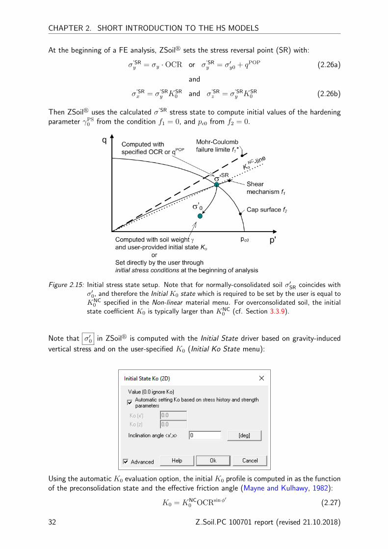
2.1.7 Initial state variables
Setting the initial stress state is necessary for calculating the initial values of hardeningparameters γPS and pc0. This calculation can be performed by a numerical procedure at thebeginning of FE analysis based on the initial effective stress conditions σ′0 = σ0(σ
′x0, σ
′y0, σ
′z0)
and its distance from the maximal stress point σ’SR which is supposed to be experiencedby the soil (see Figure 2.15). In order to calculate this distance, the user has to define thefollowing variables:
1. Stress history variable which can be set in two ways:
• through the overconsolidation ratio OCR = σvc/σ′v0 where σvc is the vertical pre-
consolidation stress (see Figure 2.13). By applying this option, a constant OCR profileis obtained.
• through the maximal preoverburden pressure offset qPOP = σvc − σ′v0 (see Figure
2.13). This option is useful to describe the deposits with varying OCR over the depth(typically superficial layers of natural soil subject to mechanical overconsolidation ordessication).
2. Historical coefficient of earth pressure at rest KSR0 which corresponds to
the maximal stress point σ’SR (Figure 2.15), and its value can be assumed as:
• KNC0 consolidation: KSR
0 = KNC0 (automatically copied from KNC
0 cell), applicableto most study cases if soil was subject to KNC
0 natural consolidation (oedometricconditions), or for simulating a triaxial compression or extension triaxial on a KNC
0 -consolidated sample.
• Isotropic consolidation: KSR0 = 1 (automatically assigned) when simulating isotropi-
cally consolidated compression or extension triaxial tests.
• Anisotropic consolidation: KSR0 (user-defined) in situations when historical consoli-
dation was different than KNC0 -consolidation specified for Eref
oed.
3. Current in situ stress configuration σ′0 = σ′0(σ′x0, σ
′y0, σ
′z0)
σ′y0 = ρ ·g · y
σ′x0 = σ′y0· K0x
σ′z0 = σ′y0· K0x
30 Z Soil.PC 100701 report (revised 21.10.2018)

2.1. HARDENING SOIL-STANDARD MODEL
Figure 2.13: Definition the initial preconsolidation state by means of a constant OCR and theresulting vertical preconsolidation stress σvc.
Figure 2.14: Definition the initial preconsolidation state by means of preoverburden pressure qPOP
and the resulting variable OCR profile (typically observed for superficial soil layers).In such a case, a variable K0 can also be considered by applying, for instance, Eq.(3.89).
Z Soil.PC 100701 report (revised 21.10.2018) 31
CHAPTER 2. SHORT INTRODUCTION TO THE HS MODELS
At the beginning of a FE analysis, ZSoilr sets the stress reversal point (SR) with:
σ’SRy = σy ·OCR or σ’SR
y = σ′y0 + qPOP (2.26a)
and
σ’SRx = σ’SR
y KSR0 and σ’SR
z = σ’SRy KSR
0 (2.26b)
Then ZSoilr uses the calculated σ’SR stress state to compute initial values of the hardeningparameter γPS0 from the condition f1 = 0, and pc0 from f2 = 0.
Figure 2.15: Initial stress state setup. Note that for normally-consolidated soil σ′SR coincides withσ′0, and therefore the Initial K0 state which is required to be set by the user is equal toKNC
0 specified in the Non-linear material menu. For overconsolidated soil, the initialstate coefficient K0 is typically larger than KNC
0 (cf. Section 3.3.9).
Note that σ′0 in ZSoilr is computed with the Initial State driver based on gravity-induced
vertical stress and on the user-specified K0 (Initial Ko State menu):
Using the automatic K0 evaluation option, the initial K0 profile is computed in as the functionof the preconsolidation state and the effective friction angle (Mayne and Kulhawy, 1982):
K0 = KNC0 OCRsinφ′ (2.27)
32 Z Soil.PC 100701 report (revised 21.10.2018)
2.1. HARDENING SOIL-STANDARD MODEL
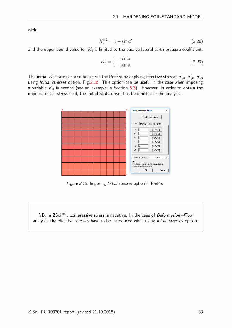
with:
KNC0 = 1− sinφ′ (2.28)
and the upper bound value for K0 is limited to the passive lateral earth pressure coefficient:
Kp =1 + sinφ
1− sinφ(2.29)
The initial K0 state can also be set via the PrePro by applying effective stresses σ′x0, σ′y0 ,σ′z0using Initial stresses option, Fig.2.16. This option can be useful in the case when imposinga variable K0 is needed (see an example in Section 5.3). However, in order to obtain theimposed initial stress field, the Initial State driver has be omitted in the analysis.
Figure 2.16: Imposing Initial stresses option in PrePro.
NB. In ZSoilr , compressive stress is negative. In the case of Deformation+Flowanalysis, the effective stresses have to be introduced when using Initial stresses option.
Z Soil.PC 100701 report (revised 21.10.2018) 33

CHAPTER 2. SHORT INTRODUCTION TO THE HS MODELS
2.1.8 Troubleshooting for Initial State analysis
It may happen that the FE analysis does not converge using the Initial State driver. In sucha case the following double-check sequence is suggested to be performed:
1. Control whether Initial K0 State is specified for each material which is defined by thematerial formulation Hardening-Soil.
2. Control whether K0 defined in Initial K0 State is larger than KSR0 defined in Non linear
menu of the HS-small strain stiffness model.
3. Try to start Initial State analysis from a very small Initial load factor (e.g. 0.2) applyinga very small Increment (e.g. 0.1 to 0.4, see below).
Another efficient way to converge and accelerate the initial state analysis is to definethe initial stress state via the PrePro by means of Initial stresses option (see Fig.2.17). In theInitial stresses dialog window, you can put default values for the simplified stress definitionwhich is applied on the whole model domain (i.e. all the soil layers). This option will helpto find the first guess but the final solution for each soil layer will be computed based on theuser-imposed K0 defined locally in the material definition, Fig. 2.1.7.
Figure 2.17: Defining initial stresses using the simplified definition.
34 Z Soil.PC 100701 report (revised 21.10.2018)
2.2. HARDENING SOIL-SMALLSTRAIN MODEL
2.2 Hardening Soil-SmallStrain model
The basic Hardening Soil-Standard model which is implemented in ZSoilr can be extendedwith the Hardening Soil-SmallStrain model which allows accounting for S-shaped stiffnessreduction which is presented in Figure 1.1. In such a case the stress paths which return tothe elastic domain during unloading can be modeled as a non-linear stress-strain relationship3.
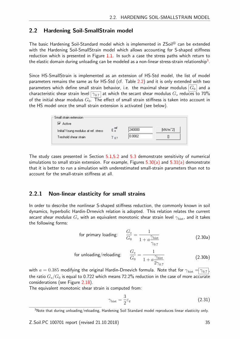
Since HS-SmallStrain is implemented as an extension of HS-Std model, the list of modelparameters remains the same as for HS-Std (cf. Table 2.2) and it is only extended with two
parameters which define small strain behavior, i.e. the maximal shear modulus G0 and acharacteristic shear strain level γ0.7 at which the secant shear modulus Gs reduces to 70%
of the initial shear modulus G0. The effect of small strain stiffness is taken into account inthe HS model once the small strain extension is activated (see below).
The study cases presented in Section 5.1,5.2 and 5.3 demonstrate sensitivity of numericalsimulations to small strain extension. For example, Figures 5.30(a) and 5.31(a) demonstratethat it is better to run a simulation with underestimated small-strain parameters than not toaccount for the small-strain stiffness at all.
2.2.1 Non-linear elasticity for small strains
In order to describe the nonlinear S-shaped stiffness reduction, the commonly known in soildynamics, hyperbolic Hardin-Drnevich relation is adopted. This relation relates the currentsecant shear modulus Gs with an equivalent monotonic shear strain level γhist, and it takesthe following forms:
for primary loading:Gs
G0
=1
1 + aγhistγ0.7
(2.30a)
for unloading/reloading:Gs
G0
=1
1 + aγhist2γ0.7
(2.30b)
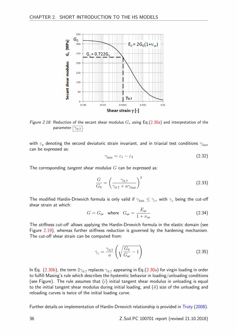
with a = 0.385 modifying the original Hardin-Drnevich formula. Note that for γhist = γ0.7 ,
the ratio Gs/G0 is equal to 0.722 which means 72.2% reduction in the case of more accurateconsiderations (see Figure 2.18).The equivalent monotonic shear strain is computed from:
γhist =3
2εq (2.31)
3Note that during unloading/reloading, Hardening Soil Standard model reproduces linear elasticity only.
Z Soil.PC 100701 report (revised 21.10.2018) 35
CHAPTER 2. SHORT INTRODUCTION TO THE HS MODELS
Figure 2.18: Reduction of the secant shear modulus Gs using Eq.(2.30a) and interpretation of theparameter γ0.7 .
with εq denoting the second deviatoric strain invariant, and in triaxial test conditions γhistcan be expressed as:
γhist = ε1 − ε3 (2.32)
The corresponding tangent shear modulus G can be expressed as:
G
G0
=
(γ0.7
γ0.7 + aγhist
)2
(2.33)
The modified Hardin-Drnevich formula is only valid if γhist ≤ γc, with γc being the cut-offshear strain at which:
G = Gur where Gur =Eur
1 + νur
(2.34)
The stiffness cut-off allows applying the Hardin-Drnevich formula in the elastic domain (seeFigure 2.19), whereas further stiffness reduction is governed by the hardening mechanism.The cut-off shear strain can be computed from:
γc =γ0.7a
(√G0
Gur− 1
)(2.35)
In Eq. (2.30b), the term 2γ0.7 replaces γ0.7 appearing in Eq.(2.30a) for virgin loading in orderto fulfill Masing’s rule which describes the hysteretic behavior in loading/unloading conditions(see Figure). The rule assumes that (i) initial tangent shear modulus in unloading is equalto the initial tangent shear modulus during initial loading, and (ii) size of the unloading andreloading curves is twice of the initial loading curve.
Further details on implementation of Hardin-Drnevich relationship is provided in Truty (2008).
36 Z Soil.PC 100701 report (revised 21.10.2018)
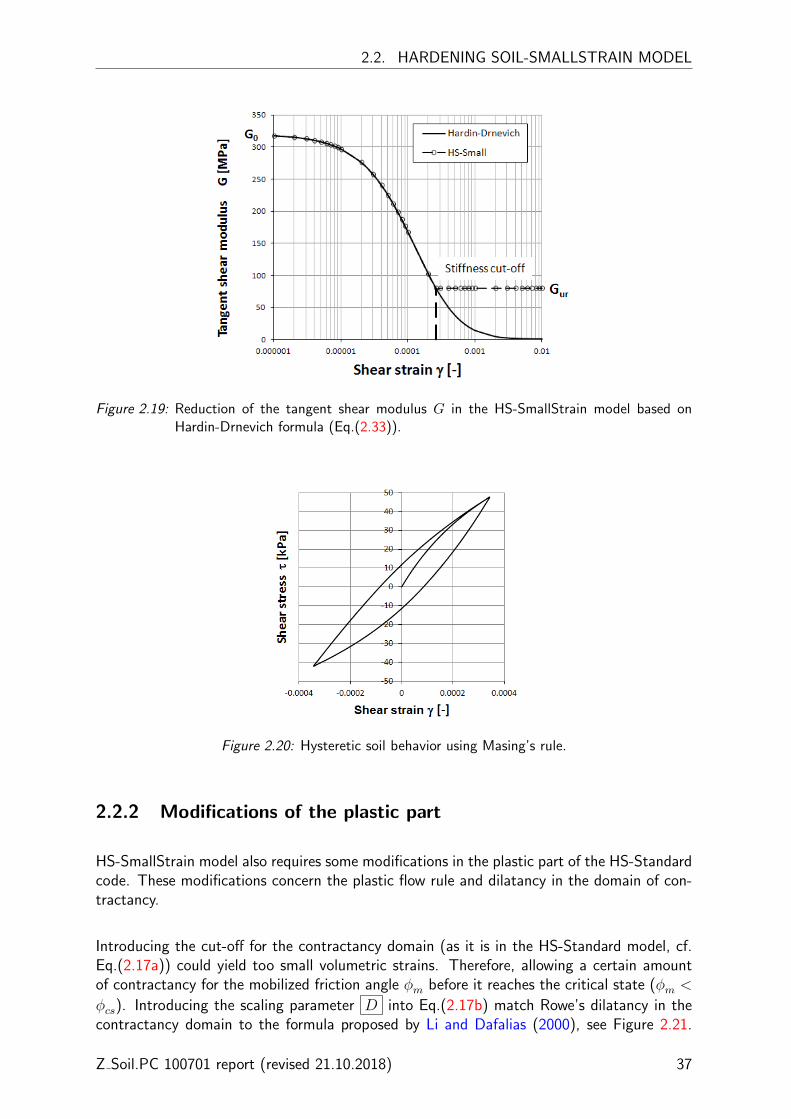
2.2. HARDENING SOIL-SMALLSTRAIN MODEL
Figure 2.19: Reduction of the tangent shear modulus G in the HS-SmallStrain model based onHardin-Drnevich formula (Eq.(2.33)).
Figure 2.20: Hysteretic soil behavior using Masing’s rule.
2.2.2 Modifications of the plastic part
HS-SmallStrain model also requires some modifications in the plastic part of the HS-Standardcode. These modifications concern the plastic flow rule and dilatancy in the domain of con-tractancy.
Introducing the cut-off for the contractancy domain (as it is in the HS-Standard model, cf.Eq.(2.17a)) could yield too small volumetric strains. Therefore, allowing a certain amountof contractancy for the mobilized friction angle φm before it reaches the critical state (φm <
φcs). Introducing the scaling parameter D into Eq.(2.17b) match Rowe’s dilatancy in thecontractancy domain to the formula proposed by Li and Dafalias (2000), see Figure 2.21.
Z Soil.PC 100701 report (revised 21.10.2018) 37

CHAPTER 2. SHORT INTRODUCTION TO THE HS MODELS
Figure 2.21: Scaled Rowe’s dilatancy vs the formula proposed by Li and Dafalias (2000).
Rowe’s dilatancy law for HS-SmallStrain model is thus formulated as:
sinψm = Dsinφm − sinφcs
1− sinφm sinφcs(2.36a)
where:
D = 0.25 if sinψm < sinφcs (2.36b)
D = 1.00 if sinψm ≥ sinφcs (2.36c)
Parameter D is automatically updated to the value 0.25, once the small strain extension isactivated.
Another modification concerns the hardening laws for parameters γPS and pc. The modifica-tion is executed by introducing hi function which is required for an appropriate approximationof γ −G curve in the case when a stress path starts directly from one or two yield surfaces.Evolution of the hardening parameters is defined as follows:
dγPS = dλ1hi
(∂g1∂σ1
− ∂g1∂σ2
− ∂g1∂σ3
)= dλ1hi for shear mechanism (2.37)
and
dpc = dλ22Hhi
(pc + c cotφ
σref + c cotφ
)2
p for volumetric mechanism (2.38)
38 Z Soil.PC 100701 report (revised 21.10.2018)

2.2. HARDENING SOIL-SMALLSTRAIN MODEL
with the function hi being defined as:
hi = G1+
Eur
2E50m (2.39)
where the stiffness multiplier Gm is calculated as:
Gm =Gmin
Gur(2.40)
with the minimum stiffness in loading history:
Gmin =G0
1 + aγmaxhist
γ0.7
(2.41)
By substituting Eq.(2.41) into Eq.(2.40), the following formula can be obtained:
Gm =G0/Gur
1 + aγmaxhist
γ0.7
=Eref
0 /Erefur
1 + aγmaxhist
γ0.7
(2.42)
Z Soil.PC 100701 report (revised 21.10.2018) 39

CHAPTER 2. SHORT INTRODUCTION TO THE HS MODELS
Table 2.2: List of parameters defining the HS-Standard ans HS-SmallStrain models.
Parameter Unit HS-Std. HS-SmallStrain
Function
Eref0 [kPa] – 3 defines the initial tangent slope of ε1 − q curve
at the reference minor principal stress σref3
γ0.7 [–] – 3 defines a characteristic shear strain level γs atwhich the ratio Gs/G0 = 0.722
Erefur [kPa] 3 3 defines unloading/reloading stiffness at engi-
neering strains (ε ≈ 10−3) at the reference mi-nor principal stress σref
3
Eref50 [kPa] 3 3 defines the secant stiffness at 50% of the ulti-
mate deviatoric stress qf at the reference minorprincipal stress σref
3
σref [kPa] 3 3 reference stress used to scale stiffness moduliEref
0 , Erefur , Eref
50 to current values with respect toa current minor principal stress σ3 (or a currentmean stress p′ if this formulation is selected)
m [–] 3 3 defines stress dependent stiffness throughEq.(2.5)
νur [–] 3 3 defines the ratio ε3/ε1 in an unloading-reloadingcycle (elastic deformations)
Rf [–] 3 3 used to compute the hardening parameter γPS
with the use of the asymptotic deviatoric stressqa defining the hyperbolic function f2 (defaultRf = 0.9)
c′ [kPa] 3 3 defines the intercept of the Mohr-Coulomb lineat null stress condition
φ′ [o] 3 3 defines the slope of the Mohr-Coulomb yield cri-terion
ψ [o] 3 3 defines the maximal slope of ε1 − εv curve fordilatancy
emax [–] 3 3 defines the cut-off limit corresponding to themaximal void ratio observed in material at theultimate state
ft [kPa] 3 3 defines the maximal tensile strength for materialD [–] 3 3 controls Rowe’s dilatancy law in the contrac-
tancy domain (default D = 0 for HS-Std, D =0.25 for HS-SmallStrain)
M [–] 3 3 defines the shape of the elliptical cap yield sur-face
H [kPa] 3 3 defines the rate of the plastic volumetric strainand the preconsolidation pressure
OCR or qPOP [–] or [kPa] 3 3 sets the initial position of stress with respect tothe cap surface and it is used to compute thehardening parameter γPS and pc0
KSR0 [–] 3 3 sets a historical position of the stress point σ’SR
(KSR0 = σ’SR
h /σ’SRv ) with respect to the initial
stress configuration for an overconsolidated ma-terial and it is used to compute the hardeningparameter γPS and and pc0
40 Z Soil.PC 100701 report (revised 21.10.2018)
2.2. HARDENING SOIL-SMALLSTRAIN MODEL
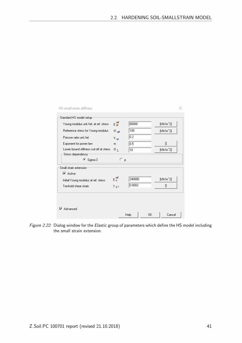
Figure 2.22: Dialog window for the Elastic group of parameters which define the HS model includingthe small strain extension.
Z Soil.PC 100701 report (revised 21.10.2018) 41

CHAPTER 2. SHORT INTRODUCTION TO THE HS MODELS
Figure 2.23: Dialog window for the Nonlinear group of parameters which define the HS modelincluding the initial state setup.
42 Z Soil.PC 100701 report (revised 21.10.2018)

2.3. MODEL PARAMETERS
2.3 Model parameters
Although the HS model is mathematically complex, its parameters have the physical meaningand they can be derived from the standard laboratory test, i.e. the triaxial compression andoedometer tests. A complete list of parameters that the user needs to specify before runningapplication is provided in Table 2.2. The details related to the identification of specific pa-rameters are provided in the subsequent Chapter 3.
The following abbreviations apply to Table 2.3:
• CICD - triaxial test: consolidated isotropically compression drained
• CICU - triaxial test: consolidated isotropically compression undrained
• OED - oedometer test
• CPT - cone penetration test
• CPTU - piezocone cone penetration test
• DMT - Marchetti’s dilatometer test
• SCPTU - piezocone cone penetration test with seismic sensor
• DMT - Marchetti’s dilatometer test with seismic sensor
• SPT - standard penetration test
Z Soil.PC 100701 report (revised 21.10.2018) 43

CHAPTER 2. SHORT INTRODUCTION TO THE HS MODELS
Table 2.3: List of parameters which should be provided by the user (advanced parameters in gray).
Model Direct estimation Alternativeparameter Unit test test or solution
Small stiffness (HS-SmallStrain only)
Eref0 [kPa] SCPT, DMT or bore-hole,
cross-hole or other geophys-ical method
unloading-reloading branchof CICD; geotechnical evi-dence; sands: CPT
γ0.7 [–] CICD with local gauges geotechnical evidence
Elastic constants
Eref50 (σref) [kPa] min. 1 CICD at σref
3 sands: CPTEref
ur (σref) [kPa] min. 1 CICD at σref3
geotechnical evidenceσref [kPa] 1 CICDνur [–] min. 1 CICD with
unloading-reloding curvegeotechnical evidence
m [–] 3 CICD at different σ3 geotechnical evidence
Shear mechanism
c [kPa] 3 CICD or CICU at differentσ3
φ [o] 3 CICD or CICU at differentσ3
geotechnical evidence; sand:CPT, DMT, PMT, SPT
ψ [o] min. 1 CICD geotechnical evidenceRf [–] min. 1 CICD default Rf = 0.9, geotech-
nical evidenceemax [–] min. 1 CICD on a dense
or preconsolidated soil spec-imen
geotechnical evidence
ft [kPa] isotropic extension default ft = 0D [–] min. 1 CICD default D=0 for HS-
Standard and D=0.25HS-SmallStrain
Volumetric (cap) mechanism
Erefoed(σref
oed) [kPa] min.1 OED clays: CPT, DMTσref
oed [kPa] idem idem
Initial state variables (soil history)
OCR or qPOP [–/kPa] min. 1 OED clay: CPT, CPTU, DMTKSR
0 [–] K0-consolidation ”Jaky’s formula”
44 Z Soil.PC 100701 report (revised 21.10.2018)
2.3. MODEL PARAMETERS
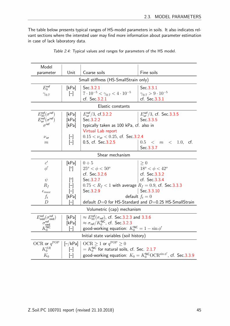
The table below presents typical ranges of HS-model parameters in soils. It also indicates rel-vant sections where the intersted user may find more information about parameter estimationin case of lack laboratory data.
Table 2.4: Typical values and ranges for parameters of the HS model.
Modelparameter Unit Coarse soils Fine soils
Small stiffness (HS-SmallStrain only)
Eref0 [kPa] Sec.3.2.1 Sec.3.3.1
γ0.7 [–] 7 · 10−5 < γ0.7 < 4 · 10−5 γ0.7 > 9 · 10−5
cf. Sec.3.2.1 cf. Sec.3.3.1
Elastic constants
Eref50 (σref) [kPa] Eref
ur /3, cf.3.2.2 Erefur /3, cf. Sec.3.3.5
Erefur (σref) [kPa] Sec.3.2.2 Sec.3.3.5σref [kPa] typically taken as 100 kPa, cf. also in
Virtual Lab reportνur [–] 0.15 < νur < 0.25, cf. Sec.3.2.4m [–] 0.5, cf. Sec.3.2.5 0.5 < m < 1.0, cf.
Sec.3.3.7
Shear mechanism
c′ [kPa] 0÷ 5 ≥ 0φ′ [o] 25o < φ < 50o 18o < φ < 42o
cf. Sec.3.2.6 cf. Sec.3.3.2ψ [o] Sec.3.2.7 cf. Sec.3.3.4Rf [–] 0.75 < Rf < 1 with average Rf = 0.9, cf. Sec.3.3.3emax [–] Sec.3.2.9 Sec.3.3.10ft [kPa] default ft = 0D [–] default D=0 for HS-Standard and D=0.25 HS-SmallStrain
Volumetric (cap) mechanism
Erefoed(σref
oed) [kPa] ≈ Eref50 (σref), cf. Sec.3.2.3 and 3.3.6
σrefoed [kPa] ≈ σref/K
NC0 , cf. Sec.3.2.3
KNC0 [–] good-working equation: KNC
0 = 1− sinφ′
Initial state variables (soil history)
OCR or qPOP [–/kPa] OCR ≥ 1 or qPOP ≥ 0KSR
0 [–] = KNC0 for natural soils, cf. Sec. 2.1.7
K0 [–] good-working equation: K0 = KNC0 OCRsinφ′ , cf. Sec.3.3.9
Z Soil.PC 100701 report (revised 21.10.2018) 45

CHAPTER 2. SHORT INTRODUCTION TO THE HS MODELS
46 Z Soil.PC 100701 report (revised 21.10.2018)

Chapter 3
Parameter determination
As most of the constitutive models for soils, the Hardening-Soil Standard model has beendesigned based on behavior of soil specimen which is observed during laboratory tests withthe use of standard devices such as triaxial cell and oedometer. Therefore, still respondingto certain test requirements such as drained compression, model parameters can be deriveddirectly from the experimental curves. Direct parameter identification is presented in Section3.1. Sometimes, the test requirements cannot be fulfilled (e.g. performing drained compres-sion test on low permeable clay specimen may prove to be too time consuming). Then, themodel can still be calibrated using, for instance, the measurements derived from the undrainedtriaxial compression test or the model parameters can be estimated based on results obtainedthrough in situ tests or approximated using parameter correlations observed in geotechnicalpractice. Such an indirect parameter determination is presented in Section 3.2 for sand typematerials, and in Section 3.3 for cohesive soils.Additional parameter which describes the small stain stiffness in the Hardening-Soil Smallmodel can be easily determined using the measurements derived from one of the in situ probesequipped with a seismic sensor which allows measuring the velocity of shear waves. Owing totime and economical constraints of laboratory testing, and the effect of specimen disturbancesduring soil sampling, the use of laboratory devices to determine G0 seems less reasonable.Nevertheless, an approximate value of G0 can be derived from unloading-reloading branchderived from the triaxial compression test.
The following sections provide a comprehensive guideline on parameter identification whichmay help the user to effectively apply the advanced constitutive models. In this context,the guideline may be helpful in specifying an appropriate testing program or making use ofalready acquired experimental results which need a specific treatment in order to estimatemodel parameters.
CHAPTER 3. PARAMETER DETERMINATION
3.1 Experimental testing requirements for direct parameter identi-fication
3.1.1 Direct parameter identification for the Hardening-Soil Stan-dard
Direct parameter identification for the Hardening-Soil Standard model requires the use of twocommonly used laboratory devices:
• triaxial cell with consolidated isotropically drained compression test (CICD); three pro-grammed compression tests at different confining pressures σ3 should provide:
F stress paths in p′ − q plane which are used to determine strength parameters φ (= φ′)
and c (= c′), according to Figure 3.1 or Mohr’s circles;Note that φ and c can also be derived from the undrained compression test1 (CU)considering that the failure stress envelopes derived from drained and undrained testsare essentially similar, see an example in Figure 3.2;
F relationships ε1 − q which is used to determine unloading-reloding modulus Eur2,3, as
shown in Figure 3.4; secant modulus E50 and failure ratio Rf according to Figure 3.3;
and stiffness stress dependency parameter m according to Figure 3.5;
F relationships ε1−εv which is used to determine the dilatancy angle ψ and the maximalvoid ratio emax , as shown in Figure 3.6.
• oedometer; the test should provide pre- and post-yield evolution of the void ratio (orspecimen height) with respect to changes of vertical effective stress, σ′v − e, which is usedto estimate:
F the preconsolidation pressure σ′c for cohesive deposits, which is then used to determine
the overconsolidation ratio OCR defined as:
OCR =σ′cσ′v0
(3.1)
F the tangent oedometric stiffness Eoed for corresponding σrefoed which have to be cap-
tured from the primary loading curve4 (postyield branch), see Figure 3.7.
The preconsolidation pressure σ′c understood as a threshold point beyond which the importantplastic straining occur, is difficult to establish unambiguously. Among a number of methodsproposed in literature for determining σ′c, the following ones are commonly used owing totheir simplicity:
1In the case of the undrained test, the maximum principal stress ratio (σ′1/σ′3)max and the maximum
deviatoric stress (σ1 − σ3)max can be considered as the failure criteria.2Note that Eur corresponds to Young’s modulus E which is specified by the user in Mohr-Coulomb or
Cap model.3Note that E0 > Eur > E50 or G0 > Gur > G50.4This condition implies that at given oedometric pressure, both shear and volumetric mechanisms are
active following KNC0 consolidation line, as shown in Figure 3.7(b).
48 Z Soil.PC 100701 report (revised 21.10.2018)
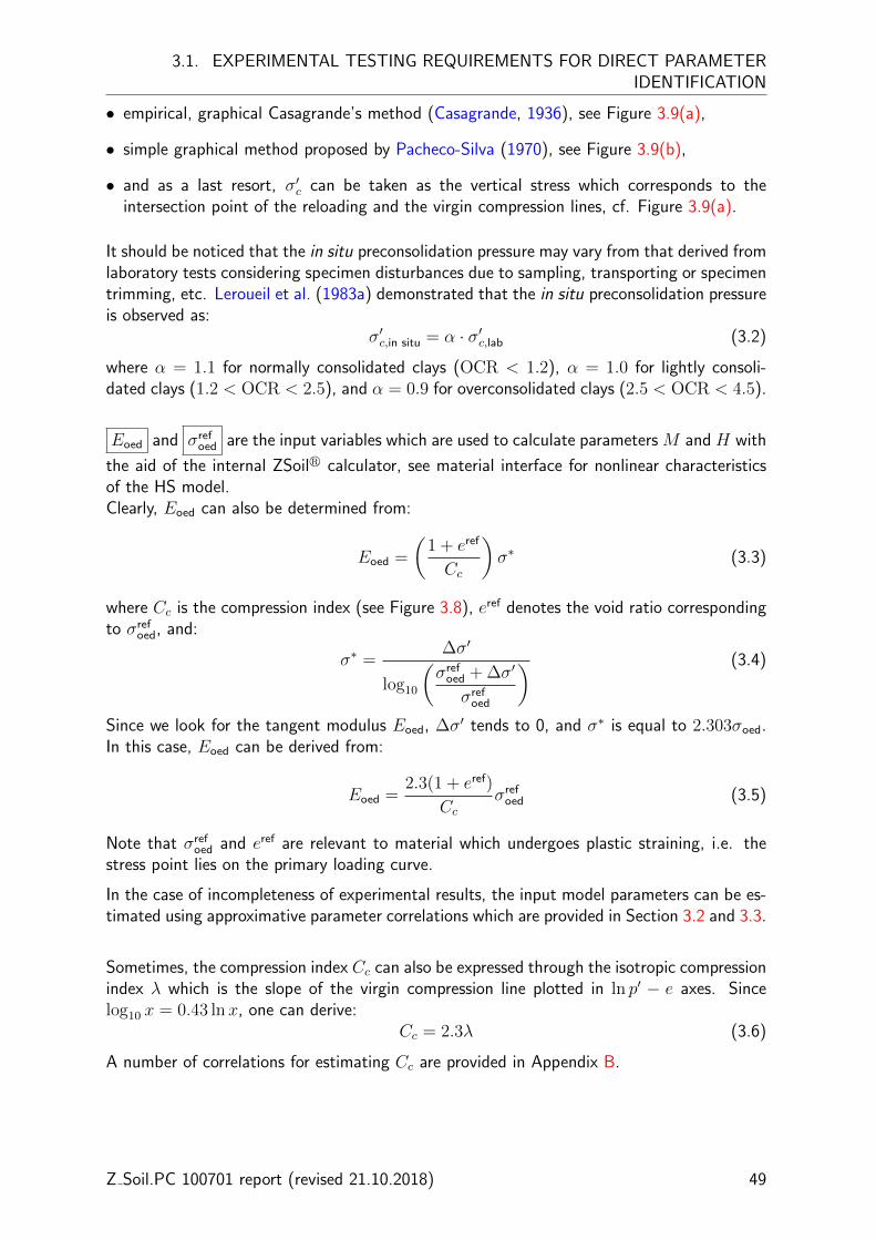
3.1. EXPERIMENTAL TESTING REQUIREMENTS FOR DIRECT PARAMETERIDENTIFICATION
• empirical, graphical Casagrande’s method (Casagrande, 1936), see Figure 3.9(a),
• simple graphical method proposed by Pacheco-Silva (1970), see Figure 3.9(b),
• and as a last resort, σ′c can be taken as the vertical stress which corresponds to theintersection point of the reloading and the virgin compression lines, cf. Figure 3.9(a).
It should be noticed that the in situ preconsolidation pressure may vary from that derived fromlaboratory tests considering specimen disturbances due to sampling, transporting or specimentrimming, etc. Leroueil et al. (1983a) demonstrated that the in situ preconsolidation pressureis observed as:
σ′c,in situ = α · σ′c,lab (3.2)
where α = 1.1 for normally consolidated clays (OCR < 1.2), α = 1.0 for lightly consoli-dated clays (1.2 < OCR < 2.5), and α = 0.9 for overconsolidated clays (2.5 < OCR < 4.5).
Eoed and σrefoed are the input variables which are used to calculate parameters M and H with
the aid of the internal ZSoilr calculator, see material interface for nonlinear characteristicsof the HS model.Clearly, Eoed can also be determined from:
Eoed =
(1 + eref
Cc
)σ∗ (3.3)
where Cc is the compression index (see Figure 3.8), eref denotes the void ratio correspondingto σref
oed, and:
σ∗ =∆σ′
log10
(σref
oed + ∆σ′
σrefoed
) (3.4)
Since we look for the tangent modulus Eoed, ∆σ′ tends to 0, and σ∗ is equal to 2.303σoed.In this case, Eoed can be derived from:
Eoed =2.3(1 + eref)
Ccσref
oed (3.5)
Note that σrefoed and eref are relevant to material which undergoes plastic straining, i.e. the
stress point lies on the primary loading curve.
In the case of incompleteness of experimental results, the input model parameters can be es-timated using approximative parameter correlations which are provided in Section 3.2 and 3.3.
Sometimes, the compression index Cc can also be expressed through the isotropic compressionindex λ which is the slope of the virgin compression line plotted in ln p′ − e axes. Sincelog10 x = 0.43 lnx, one can derive:
Cc = 2.3λ (3.6)
A number of correlations for estimating Cc are provided in Appendix B.
Z Soil.PC 100701 report (revised 21.10.2018) 49
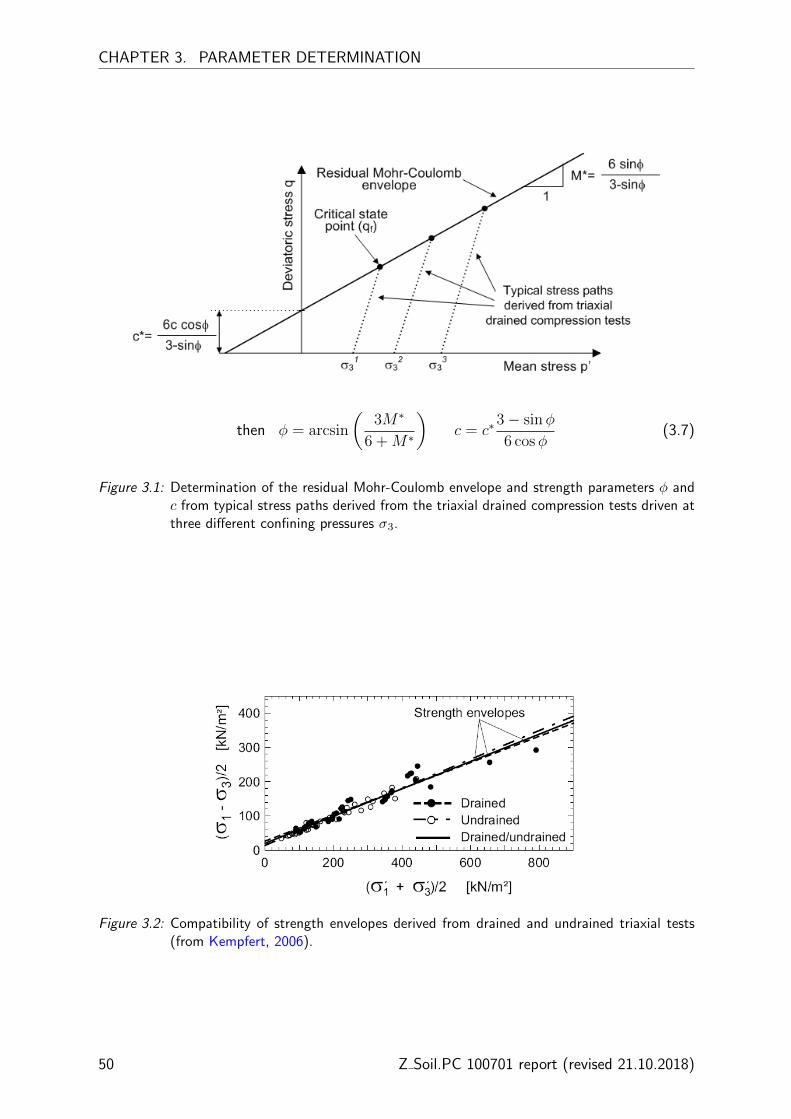
CHAPTER 3. PARAMETER DETERMINATION
then φ = arcsin
(3M∗
6 +M∗
)c = c∗
3− sinφ
6 cosφ(3.7)
Figure 3.1: Determination of the residual Mohr-Coulomb envelope and strength parameters φ andc from typical stress paths derived from the triaxial drained compression tests driven atthree different confining pressures σ3.
Figure 3.2: Compatibility of strength envelopes derived from drained and undrained triaxial tests(from Kempfert, 2006).
50 Z Soil.PC 100701 report (revised 21.10.2018)

3.1. EXPERIMENTAL TESTING REQUIREMENTS FOR DIRECT PARAMETERIDENTIFICATION
Figure 3.3: Determination of the slope a and b for identification of the secant modulus E50 andfailure ratio Rf from typical triaxial drained compression results ε1 − q. Best precisionof the interpreted parameters is obtained by plotting the trendline for two closest datapoints adjacent to 0.5qf .
Figure 3.4: Determination of E moduli (input model parameters) from a typical curve derived fromthe triaxial drained compression tests.
Z Soil.PC 100701 report (revised 21.10.2018) 51
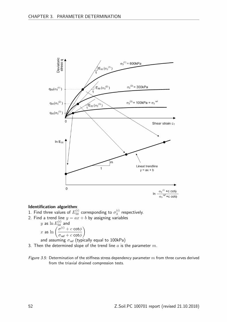
CHAPTER 3. PARAMETER DETERMINATION
Identification algorithm:1. Find three values of E
(i)50 corresponding to σ
(i)3 respectively.
2. Find a trend line y = ax+ b by assigning variablesy as lnE
(i)50 and
x as ln
(σ(i) + c cotφ
σref + c cotφ
)and assuming σref (typically equal to 100kPa)
3. Then the determined slope of the trend line a is the parameter m.
Figure 3.5: Determination of the stiffness stress dependency parameter m from three curves derivedfrom the triaxial drained compression tests.
52 Z Soil.PC 100701 report (revised 21.10.2018)
3.1. EXPERIMENTAL TESTING REQUIREMENTS FOR DIRECT PARAMETERIDENTIFICATION
ψ = − arcsin
(d
2− d
)assuming negative sign (-) for an increase of the specimen hight
and compressive axial strain with positive sign (+)
Figure 3.6: Determination of the dilatancy angle ψ from εv − ε1 curve obtained in the triaxialdrained compression test.
p∗ =1 + 2KNC
0
3σref
oed and q∗ = (1−KNC0 )σref
oed
(a) (b)
Figure 3.7: Assumptions to the automatic determination of parameters M and H: at given σrefoed
which is located at post-yield plastic curve, both shear an volumetric mechanism areactive.
Z Soil.PC 100701 report (revised 21.10.2018) 53
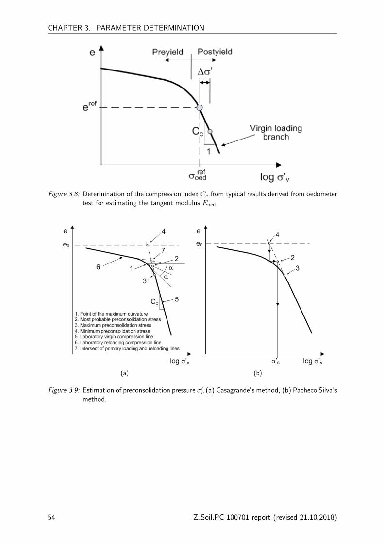
CHAPTER 3. PARAMETER DETERMINATION
Figure 3.8: Determination of the compression index Cc from typical results derived from oedometertest for estimating the tangent modulus Eoed.
(a) (b)
Figure 3.9: Estimation of preconsolidation pressure σ′c (a) Casagrande’s method, (b) Pacheco Silva’smethod.
54 Z Soil.PC 100701 report (revised 21.10.2018)

3.1. EXPERIMENTAL TESTING REQUIREMENTS FOR DIRECT PARAMETERIDENTIFICATION
3.1.2 Direct parameter identification for the Hardening-Soil Small
Direct parameter identification for the Hardening-Soil Small model requires the measurementsderived from geophysical tests or one of the advanced in situ probes equipped with a seismicsensor which allows measuring the shear wave velocity Vs in the subsoil. Two commonlyknown devices, i.e. the seismic piezocone (SCPT or SCPTU) or seismic Marchetti’sdilatometer (SDMT), can be used to determine small strain stiffness G0 (or Gmax) fromthe following expression:
G0 = ρV 2s (3.8)
where ρ is a density of soil. Typical ranges for Vs in different types of soils, as well as a varietyof methods that can be used to estimate Vs from in situ tests (SPT, DMT, CPT, PMT) aregiven in Appendix C.Note that in natural conditions G0 is stress dependent and, in the HS-SmallStrain model,this parameter is defined by analogy to other stiffness moduli with:
G0 = Gref0
(σ∗3 + c cotφ
σref + c cotφ
)m(3.9)
Having determined G0, the parameter E0 which is defined by the user in the material dialog,can be calculated from:
E0 = 2(1 + νur)G0 (3.10)
assuming that Poisson’s coefficient νur is a constant in the model.
Soil stiffness at very small strains can also be approximated based on the initial part of theε1 − q curve or the unloading-reloading branch derived from the triaxial compression test,as demonstrated on Figure 3.4. However, an exact determination of the initial soil stiffnessEi may prove to be difficult, especially in soft soils. Therefore, one should realize that theinitial slope Ei derived from triaxial test can be more than once lower than soil stiffness E0
observed in natural conditions.
Identification of the parameter γ0.7 at which the secant shear modulus Grefs is reduced to
0.722Gref0 , requires the use of advanced laboratory devices in order to determine the S-shape
curve at very small strain levels. In practice, it may prove to be time-consuming and expensiveand therefore, it is suggested to estimate γ0.7 by means of typically observed experimental
curves. In the case of granular materials γ0.7 mostly depends on the mean effective stress
p′ (see Figure 3.19 ) but also on overconsolidation. In cohesive materials, γ0.7 may mostly
depend on the plasticity index IP (PI) (see Figures 3.38 or 3.40), however the stress level(p′) and the overconsolidation (OCR) may also increase the value of γ0.7 . Having assumed
all other model parameters, it is also recommended to run a one-element simulation of thetriaxial compression test in order to examine the shape of log(ε1)−G (or E) curve derivedfrom the computed ε1 − q results.
Z Soil.PC 100701 report (revised 21.10.2018) 55

CHAPTER 3. PARAMETER DETERMINATION
3.1.3 Parameter identification sequence
The following sequence should be followed during parameter identification for the HS model:
1. Identify φ′ and c′ (e.g. Figure 3.1)
2. Identify ψ (e.g. Figure 3.6)
3. Identify Rf and E(i)50 for different confining pressures σ
(i)3 (e.g. Figure 3.3)
4. Identify E(i)ur for different confining pressures σ
(i)3 (the value of νur can be assigned between
0.1 and 0.2)
5. Identify m based on the identified values of E(i)50 or/and E
(i)ur (e.g. Figure 3.5)
6. Assign the reference stress σref (it can be the confining pressure in the triaxial test thatbest corresponds to in situ stress conditions)
7. Evaluate E0 and γ0.7
8. Calculate Eref0 , Eref
ur , Eref50 in terms of σref (note that by applying the stress stiffness depen-
dency law such as Eq.(2.4) the stiffness moduli also depend on φ, c and m)
9. Double-check the following relationships:
• Eref0 > Eref
ur > Eref50
• Erefur /E
ref50 > 2
• 3.6 < Eref0 /E
ref50 < 30 (typically 6 < Eref
0 /Eref50 < 14)
10. Evaluate KNC0 and Eref
oed for the corresponding vertical reference stress σrefoed in order to
compute M and H (note that M and H should be recomputed if one of the followingparameters has been changed: Eur, νur, m, E50, φ, ψ, c, Rf )
11. Evaluate the profile of soil preconsolidation in order to specify a constant OCR or a variableOCR profile by means of qPOP
12. Set KSR0 = KNC
0
13. Evaluate the in situ stress state in order to specify K0 (for example accounting for precon-solidation state Eq.(3.89))
An example of parameter identification using a spreadsheet is given in Table 5.8.
56 Z Soil.PC 100701 report (revised 21.10.2018)
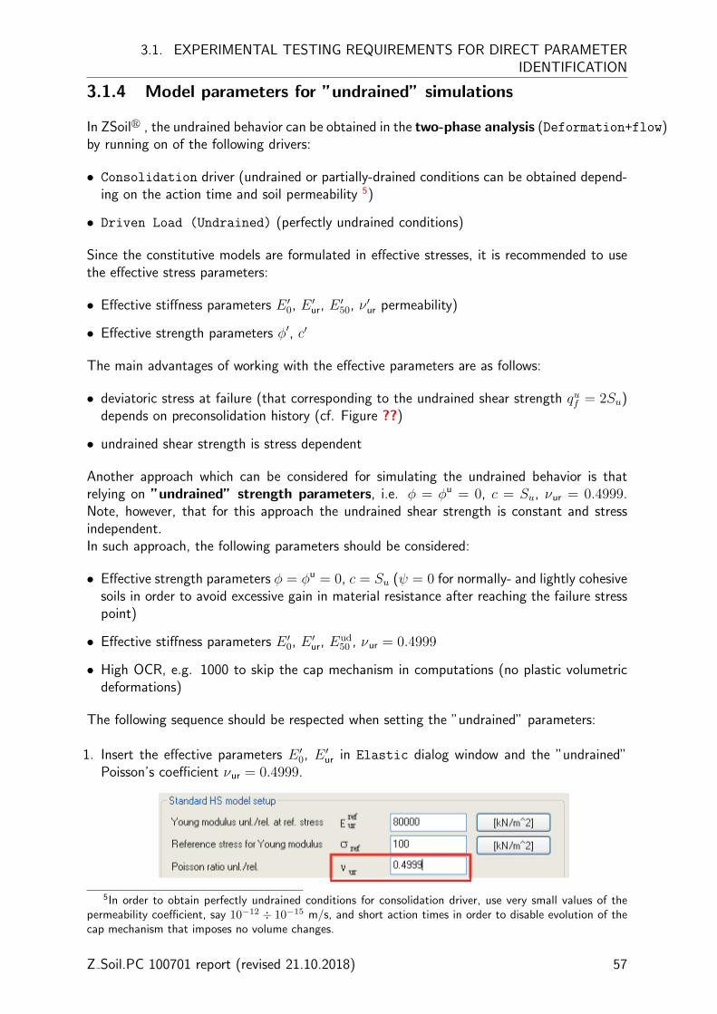
3.1. EXPERIMENTAL TESTING REQUIREMENTS FOR DIRECT PARAMETERIDENTIFICATION
3.1.4 Model parameters for ”undrained” simulations
In ZSoilr , the undrained behavior can be obtained in the two-phase analysis (Deformation+flow)by running on of the following drivers:
• Consolidation driver (undrained or partially-drained conditions can be obtained depend-ing on the action time and soil permeability 5)
• Driven Load (Undrained) (perfectly undrained conditions)
Since the constitutive models are formulated in effective stresses, it is recommended to usethe effective stress parameters:
• Effective stiffness parameters E ′0, E ′ur, E′50, ν ′ur permeability)
• Effective strength parameters φ′, c′
The main advantages of working with the effective parameters are as follows:
• deviatoric stress at failure (that corresponding to the undrained shear strength quf = 2Su)depends on preconsolidation history (cf. Figure ??)
• undrained shear strength is stress dependent
Another approach which can be considered for simulating the undrained behavior is thatrelying on ”undrained” strength parameters, i.e. φ = φu = 0, c = Su, νur = 0.4999.Note, however, that for this approach the undrained shear strength is constant and stressindependent.In such approach, the following parameters should be considered:
• Effective strength parameters φ = φu = 0, c = Su (ψ = 0 for normally- and lightly cohesivesoils in order to avoid excessive gain in material resistance after reaching the failure stresspoint)
• Effective stiffness parameters E ′0, E ′ur, Eud50 , νur = 0.4999
• High OCR, e.g. 1000 to skip the cap mechanism in computations (no plastic volumetricdeformations)
The following sequence should be respected when setting the ”undrained” parameters:
1. Insert the effective parameters E ′0, E ′ur in Elastic dialog window and the ”undrained”Poisson’s coefficient νur = 0.4999.
5In order to obtain perfectly undrained conditions for consolidation driver, use very small values of thepermeability coefficient, say 10−12 ÷ 10−15 m/s, and short action times in order to disable evolution of thecap mechanism that imposes no volume changes.
Z Soil.PC 100701 report (revised 21.10.2018) 57

CHAPTER 3. PARAMETER DETERMINATION
In the Nonlinear dialog window, disableAutomatic evaluation of H and M parameters in order to avoid unfeasible calcula-tion of M and H parameters for the null friction angle.
2. Set ”undrained” parameters φu = 0o, c = Su, and ψ = 0 for normally- and lightly cohesivesoils in order to avoid excessive gain in material resistance after reaching the failure stresspoint (cf. Truty and Obrzud (2015)).
3. Set high OCR, e.g.1000, in order to skip the cap mechanism during analysis
4. Set input E50 equal to undrained one Eu50. The ”undrained” secant modulus can be com-
puted from:
Eu50 =
3E ′502(1 + ν)
(3.11)
where ν should correspond to the ratio ε3/ε1 obtained for plastic straining and the efectivesecant modulus E ′50, i.e. ν ≈ 0.3.
58 Z Soil.PC 100701 report (revised 21.10.2018)
3.2. ALTERNATIVE PARAMETER ESTIMATION FOR GRANULAR MATERIALS
3.2 Alternative parameter estimation for granular materials
3.2.1 Initial stiffness modulus and small strain threshold
The present section provides a number of approaches for estimating the initial soil stiffnessand the small strain threshold γ0.7. Some correlations allows to directly approximate theinput parameter E0, the others provide solutions for estimating the initial shear modulus G0.Then the input parameter E0 can be obtained through:
E0 = 2(1 + νur)G0 (3.12)
assuming a constant value of the unloading-reloading Poisson’s coefficient νur.
Geotechnical evidence. Experimental data shows that the initial stiffness of soils maydepend on the stress level, soil porosity and overconsolidation. These factors can be takeninto account using a modified equation proposed by Hardin and Black (1969):
G0 = A · f(e) ·OCRk
(p′
pref
)m, in [MPa] (3.13)
where G0 is the maximum small-strain shear modulus in MPa, p′ is the mean effective stressin kPa, pref is the reference stress equal to the atmospheric pressure pref = 100 kPa, OCRis the overconsolidation ratio and A, f(e), k, m are the correlated functions and parameterswhich are given in Table 3.1 and 3.2 for different types of soils. It is observed that theempirical exponent k varies from 0 for sands and 0.5 for high plasticity clays.
Biarez and Hicher (1994) proposed a simple relationship for all soils with wL < 50%:
E0 =140
e
(p′
pref
)0.5
, in [MPa] (3.14)
Z Soil.PC 100701 report (revised 21.10.2018) 59

CHAPTER 3. PARAMETER DETERMINATION
Table 3.1: Parameters for estimation of G0 in different types of granular soils using Eq.(3.13).
Soil tested D50 Cu A f(e) k m Reference[mm] [-] [-] [-] [-] [-]
Kenya carbonate sand 0.13 1.86 101-129 e−0.8 0 0.45-0.52Fioravante (2000)
Quiou carbonate sand 0.75 4.40 71 e−1.3 0 0.62Lo Presti et al. (1993)
Ottawa sand No.20-30 0.72 1.20 69(2.17− e)2
1 + e0 0.50
Hardin and Richart Jr (1963)
SLB sand (subround) 0.62 1.11 82-130(2.17− e)2
1 + e0 0.44-0.53
Hoque and Tatsuoka (2004)
Toyoura sand (subangu-lar)
0.16 1.46 71-87(2.17− e)2
1 + e0 0.41-0.51
Hoque and Tatsuoka (2004)
Toyoura sand (subangu-lar)
0.19 1.56 84-104(2.17− e)2
1 + e0 0.50-0.57
Chaudary et al. (2004)
Toyoura sand (subangu-lar)
0.22 1.35 72 e−1.3 0 0.45Lo Presti et al. (1993)
Ticino sand (subangu-lar)
0.50 1.33 61-64(2.17− e)2
1 + e0 0.44-0.53
Hoque and Tatsuoka (2004)
Ticino sand (subangu-lar)
0.54 1.50 71(2.27− e)2
1 + e0 0.43
Lo Presti et al. (1993)
Ticino sand (subangu-lar)
0.55 1.66 79-90 e−0.8 0 0.43-0.48Fioravante (2000)
Ham River sand (suban-gular)
0.27 1.67 72-81(2.17− e)2
1 + e0 0.5-0.52
Kuwano and Jardine (2002)
Silica sand (subangular) 0.20 1.10 80(2.17− e)2
1 + e0 0.5
Kallioglou et al. (2003)
Hostun sand (angular) 0.31 1.94 80(2.17− e)2
1 + e0 0.47
Hoque and Tatsuoka (2000)
Silica sand (angular) 0.32 2.80 48(2.17− e)2
1 + e0 0.50
Kallioglou et al. (2003)
Silica sand 0.55 1.80 275(1.46− e)2
1 + e0 0.42
Wichtmann and Triantafyllidis(2004)
Hime gravel (subround) 1.73 1.33 53-94(2.17− e)2
1 + e0 0.45-0.51
Chaudary et al. (2004)
Chiba gravel (subround) 7.90 10 76(2.17− e)2
1 + e0 0.50
Modoni et al. (1999)
Table 3.2: Parameters for estimation of G0 in granular soils using Eq.(3.13).
Soil tested emin emax A f(e) m Reference[-] [-] [-] [-] [-]
Clean uniform sandswith Cu < 1.8
0.5 1.1 57(2.17− e)2
1 + e0.4 Iwasaki and Tatsuoka (1977)
All soils with wL <50%
0.4 1.8 58∗1
e0.5 Biarez and Hicher (1994)
Undisturbed crushedsands
0.6 1.5 33(2.97− e)2
1 + e0.5 Hardin and Black (1969)
∗obtained from Eq. 3.14 assuming ν = 0.2
60 Z Soil.PC 100701 report (revised 21.10.2018)
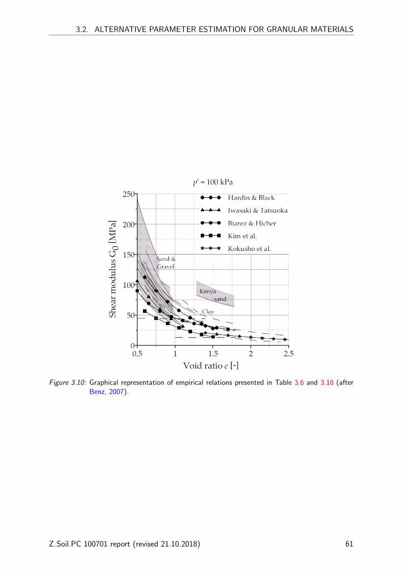
3.2. ALTERNATIVE PARAMETER ESTIMATION FOR GRANULAR MATERIALS
Figure 3.10: Graphical representation of empirical relations presented in Table 3.6 and 3.18 (afterBenz, 2007).
Z Soil.PC 100701 report (revised 21.10.2018) 61
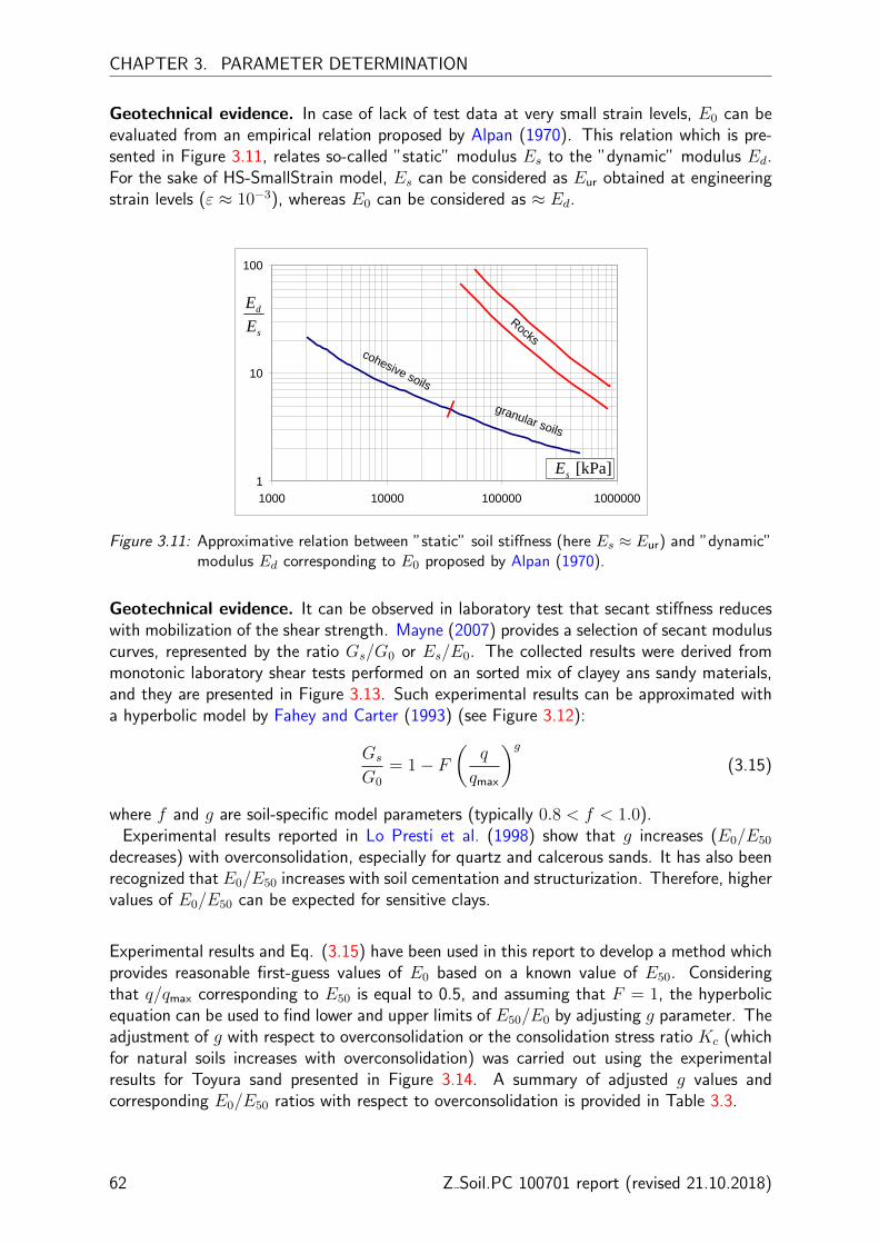
CHAPTER 3. PARAMETER DETERMINATION
Geotechnical evidence. In case of lack of test data at very small strain levels, E0 can beevaluated from an empirical relation proposed by Alpan (1970). This relation which is pre-sented in Figure 3.11, relates so-called ”static” modulus Es to the ”dynamic” modulus Ed.For the sake of HS-SmallStrain model, Es can be considered as Eur obtained at engineeringstrain levels (ε ≈ 10−3), whereas E0 can be considered as ≈ Ed.
1
10
100
1000 10000 100000 1000000
cohesive soils
granular soils
Rockss
d
EE
[kPa]sE
Figure 3.11: Approximative relation between ”static” soil stiffness (here Es ≈ Eur) and ”dynamic”modulus Ed corresponding to E0 proposed by Alpan (1970).
Geotechnical evidence. It can be observed in laboratory test that secant stiffness reduceswith mobilization of the shear strength. Mayne (2007) provides a selection of secant moduluscurves, represented by the ratio Gs/G0 or Es/E0. The collected results were derived frommonotonic laboratory shear tests performed on an sorted mix of clayey ans sandy materials,and they are presented in Figure 3.13. Such experimental results can be approximated witha hyperbolic model by Fahey and Carter (1993) (see Figure 3.12):
Gs
G0
= 1− F(
q
qmax
)g(3.15)
where f and g are soil-specific model parameters (typically 0.8 < f < 1.0).Experimental results reported in Lo Presti et al. (1998) show that g increases (E0/E50
decreases) with overconsolidation, especially for quartz and calcerous sands. It has also beenrecognized that E0/E50 increases with soil cementation and structurization. Therefore, highervalues of E0/E50 can be expected for sensitive clays.
Experimental results and Eq. (3.15) have been used in this report to develop a method whichprovides reasonable first-guess values of E0 based on a known value of E50. Consideringthat q/qmax corresponding to E50 is equal to 0.5, and assuming that F = 1, the hyperbolicequation can be used to find lower and upper limits of E50/E0 by adjusting g parameter. Theadjustment of g with respect to overconsolidation or the consolidation stress ratio Kc (whichfor natural soils increases with overconsolidation) was carried out using the experimentalresults for Toyura sand presented in Figure 3.14. A summary of adjusted g values andcorresponding E0/E50 ratios with respect to overconsolidation is provided in Table 3.3.
62 Z Soil.PC 100701 report (revised 21.10.2018)

3.2. ALTERNATIVE PARAMETER ESTIMATION FOR GRANULAR MATERIALS
Figure 3.12: Reduction of G0/G50 by the hyperbolic model - Equation (3.15) (assuming F = 1).
q/qmax = 0.5
Figure 3.13: Observed secant stiffness modulus reduction curves from static torsional and triaxialshear data on clays and sands (from Mayne, 2007) and the superposed hyperboliccurves obtained for different g values. The adjusted g values provides reasonable first-guess lower and upper limits for estimating E0 from a determined E50 value (see Table3.3).
Z Soil.PC 100701 report (revised 21.10.2018) 63

CHAPTER 3. PARAMETER DETERMINATION
q/qmax = 0.5
Figure 3.14: Normalized secant modulus of Toyura vs mobilized shear strength (Lo Presti et al.,1998, from) and adjusting of g parameter with respect to stress consolidation ratio.
Table 3.3: Typical values of E0/E50 ratio for granular soils with respect to the preconsolidationstate (this table has been developed based on literature review and Fahey’s stiffnessreduction model).
OCR [–] E0/E50 [–] Corresponding g [–]
Degree of preconsolidation ”Min” ”Max” For ”Min” For ”Max”
Unknown 4.1 18.0 0.40 0.083Normally consolidated 1÷ 1.2 6.3 18.0 0.25 0.083Lightly overconsolidated 1.2÷ 2.5 4.6 12.5 0.35 0.12Overconsolidated 2.5÷ 4.5 3.9 8.1 0.43 0.19Heavily overconsolidated 4.5÷ 10 3.6 5.5 0.47 0.29
The higher values of E0/E50 ratio are suggested for aged, cemented and structured sands.
64 Z Soil.PC 100701 report (revised 21.10.2018)
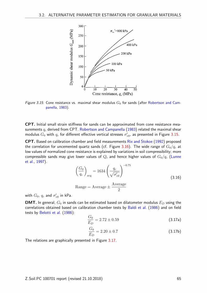
3.2. ALTERNATIVE PARAMETER ESTIMATION FOR GRANULAR MATERIALS
Figure 3.15: Cone resistance vs. maximal shear modulus G0 for sands (after Robertson and Cam-panella, 1983).
CPT. Initial small strain stiffness for sands can be approximated from cone resistance mea-surements qc derived from CPT. Robertson and Campanella (1983) related the maximal shearmodulus G0 with qc for different effective vertical stresses σ′v0, as presented in Figure 3.15.
CPT. Based on calibration chamber and field measurements Rix and Stokoe (1992) proposedthe correlation for uncemented quartz sands (cf. Figure 3.16). The wide range of G0/qc atlow values of normalized cone resistance is explained by variations in soil compressibility; morecompressible sands may give lower values of Qt and hence higher values of G0/qc (Lunneet al., 1997). (
G0
qc
)avg
= 1634
(qc√σ′v0
)−0.75
Range = Average± Average
2
(3.16)
with G0, qc and σ′v0 in kPa.
DMT. In general, G0 in sands can be estimated based on dilatometer modulus ED using thecorrelations obtained based on calibration chamber tests by Baldi et al. (1986) and on fieldtests by Belotti et al. (1986):
G0
ED= 2.72± 0.59 (3.17a)
G0
ED= 2.20± 0.7 (3.17b)
The relations are graphically presented in Figure 3.17.
Z Soil.PC 100701 report (revised 21.10.2018) 65

CHAPTER 3. PARAMETER DETERMINATION
Figure 3.16: Comparison of empirical correlations for estimating G0 (Gmax) in sands (Eq.(3.16))and clays (Eq.(3.47)) from CPT data (correlations interpreted for typical qt ranges).
Figure 3.17: Comparison of empirical correlations for estimating G0 (Gmax) in sands from DMTdata (Eq.(3.17a) and Eq.(3.17b).
66 Z Soil.PC 100701 report (revised 21.10.2018)

3.2. ALTERNATIVE PARAMETER ESTIMATION FOR GRANULAR MATERIALS
SPT. G0 can be estimated for sands from the correlation proposed by Ohta and Goto (1976,as referred in Kramer (1996)), cf. Figure 3.18:
G0 = 438N0.33331,60 pa
(p′
pa
)0.5
(3.18)
with G0 and p′-mean effective stress in kPan and pa = 100kPa, N1,60 - ”overburden-corrected” N60-value (cf. Table 3.10).
Another correlation for sand based on SPT date was proposed by Imai and Tonouchi (1982,as refered in Kramer (1996)), cf. Figure 3.18:
G0 = 15600N0.6860 (3.19)
(G0 in kPa.)
Figure 3.18: Comparison of empirical correlations for estimating G0 (Gmax) in sands from SPTdata, Eq.(3.18) plotted for K0 = 0.4 and Eq.(3.19).
Z Soil.PC 100701 report (revised 21.10.2018) 67

CHAPTER 3. PARAMETER DETERMINATION
Geotechnical evidence. It has been proved experimentally that the strain threshold γ0.7does not depend on soil density in the case of non-cohesive granular soils (cf. 3.19). On theother hand, γ0.7 can be affected by the magnitude of the confining pressure σ′0 which corre-sponds to the mean effective stress p′ for in situ conditions (cf. Darendeli and Stokoe (2001);Wichtmann and Triantafyllidis (2004)). Hence, the parameter γ0.7 can be approximated froma diagram presented in Figure 3.19. Note that the model formulation does not account forstress dependency of γ0.7. If needed this parameter can be incorporated into boundary valueproblems through definition average mean effective stress for defined sub-layers.
Figure 3.19: Influence of relative density ID and the confining pressure p′ on strain threshold γ0.7for sands (from Wichtmann and Triantafyllidis, 2004).
Experimental evidence for sands reported in Darendeli and Stokoe (2001), Figure 3.20, allowsto write the following approximating relationship:
γ0.7 = γref0.7
(p′
pa
)0.35
with
γref0.7 (pa) = 1.26 · 10−4 - reference strain threshold at pa
pa = 1atm ≈ 100kPa - atmospheric pressure
(3.20)
An estimation of γ0.7 for granular soils can also be carried out using a linear interpolationwhich is obtained through interpretation of the results presented in Figure 3.19:
γ0.7 = 8.75 · 10−5p′
pref+ γref
0.7 for p′ ≤< 400kPa
with
γref0.7
(pref)
= 1.0 · 10−4 - reference strain threshold at pref
pref = 100kPa - reference pressure
(3.21)
where pref = 100kPa.A fit of the above correlation to the experimental curves is presented in Figure 3.21.
68 Z Soil.PC 100701 report (revised 21.10.2018)
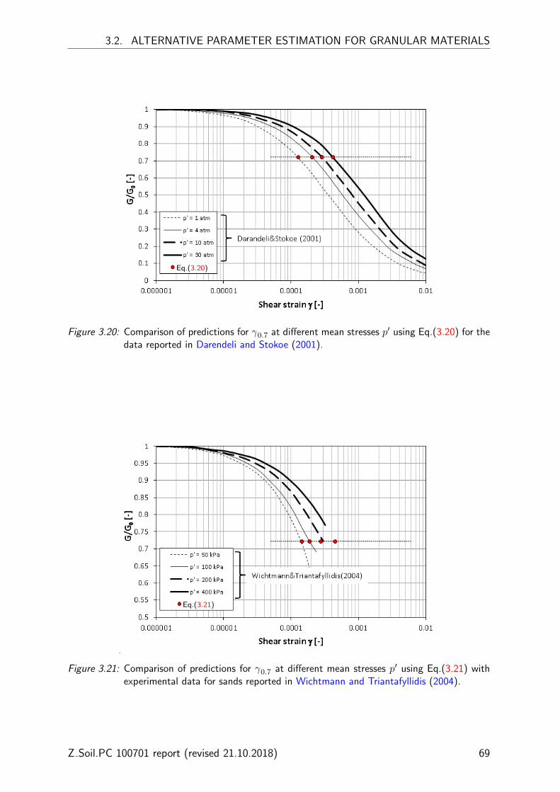
3.2. ALTERNATIVE PARAMETER ESTIMATION FOR GRANULAR MATERIALS
Eq.(3.20)
Figure 3.20: Comparison of predictions for γ0.7 at different mean stresses p′ using Eq.(3.20) for thedata reported in Darendeli and Stokoe (2001).
Eq.(3.21)
Figure 3.21: Comparison of predictions for γ0.7 at different mean stresses p′ using Eq.(3.21) withexperimental data for sands reported in Wichtmann and Triantafyllidis (2004).
Z Soil.PC 100701 report (revised 21.10.2018) 69
CHAPTER 3. PARAMETER DETERMINATION
In the case of granular soils, it is also observed that the strain threshold may be affectedby OCR and for sands with high content of fines additionally on IP . In order to accountthese effects, the correlation presented in Eq.(3.54) can be used (this generalized formulaby Darendeli (2001) was developed based on a database containing four groups of soils, i.e.”clean” sands, sands with high content of fines, silts and clays.
70 Z Soil.PC 100701 report (revised 21.10.2018)

3.2. ALTERNATIVE PARAMETER ESTIMATION FOR GRANULAR MATERIALS
3.2.2 Secant and unloading-reloading moduli
In general, the relation between the stiffness moduli is as follows:
E50 < Es < Eur (3.22)
where Es denotes ”static” modulus or secant modulus taken from the initial part of the ε1−qexperimental curve at ε1 = 0.1%.
In the case when E50 or Eur cannot be directly determined from experimental curves, it maybe relevant for many practical cases to set:
Erefur
Eref50
= 2 to 6 (an average can be assumed equal to 3) (3.23)
Higher ratios can be assumed for loose sands (3 to 6), whereas lower ones for dense sands
(2 to 4). However, note that the following condition should be satisfied:Eref
ur
Eref50
> 2.
However, note that the following condition should be satisfied:Eref
ur
Eref50
> 2.
In absence of laboratory results, the stiffness moduli can be approximated based on typicallyobserved order of magnitudes of ”static” modulus Es which are given in Table 3.4. Assumingthat soil behavior follows the stress-strain relation described by Equation 2.8 and assumingε1 = 0.1%, the ”static” modulus can be represented with:
Es =q
0.001=
11
2E50
+0.001 ·Rf
qf (φ, c)
(3.24)
The above equation can be represented graphically in Figure 3.22, and can be used to estimateE50 from the known value of Es.
Table 3.4: Typical values for the ”static” modulus Es [MPa] (compiled from Kezdi, 1974; Pratet al., 1995, and extended by the authors).
Soil Density
Very loose Loose Medium Dense Very dense
Soil Type Min Max Min Max Min Max Min Max Min Max
Gravels/Sand well-graded 10 30 30 80 80 160 160 320 320 480Sand, uniform 5 10 10 10 30 30 50 50 80 120Sand/Gravel silty 3 7 7 12 12 20 20 30 30 40Sand/Gravel clayey 2 6 6 10 10 15 15 21 21 29
Z Soil.PC 100701 report (revised 21.10.2018) 71

CHAPTER 3. PARAMETER DETERMINATION
Figure 3.22: Estimating the ratio between the static modulus Es and secant modulus E50.
For sands, the secant modulus E50 can be estimated based on the known porosity, Figure3.23.
Figure 3.23: Normalized secant modulus E50 vs. porosity n0 for different sands (after Schanz andVermeer, 1998).
72 Z Soil.PC 100701 report (revised 21.10.2018)
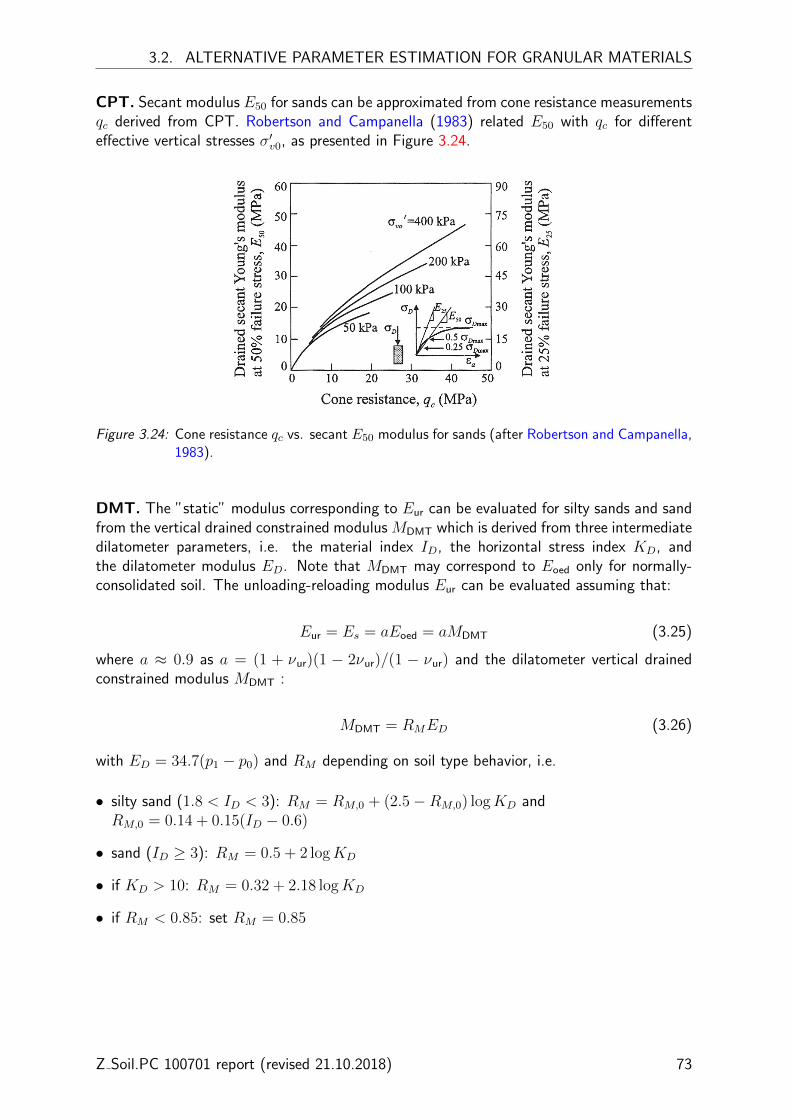
3.2. ALTERNATIVE PARAMETER ESTIMATION FOR GRANULAR MATERIALS
CPT. Secant modulus E50 for sands can be approximated from cone resistance measurementsqc derived from CPT. Robertson and Campanella (1983) related E50 with qc for differenteffective vertical stresses σ′v0, as presented in Figure 3.24.
Figure 3.24: Cone resistance qc vs. secant E50 modulus for sands (after Robertson and Campanella,1983).
DMT. The ”static” modulus corresponding to Eur can be evaluated for silty sands and sandfrom the vertical drained constrained modulus MDMT which is derived from three intermediatedilatometer parameters, i.e. the material index ID, the horizontal stress index KD, andthe dilatometer modulus ED. Note that MDMT may correspond to Eoed only for normally-consolidated soil. The unloading-reloading modulus Eur can be evaluated assuming that:
Eur = Es = aEoed = aMDMT (3.25)
where a ≈ 0.9 as a = (1 + νur)(1 − 2νur)/(1 − νur) and the dilatometer vertical drainedconstrained modulus MDMT :
MDMT = RMED (3.26)
with ED = 34.7(p1 − p0) and RM depending on soil type behavior, i.e.
• silty sand (1.8 < ID < 3): RM = RM,0 + (2.5−RM,0) logKD andRM,0 = 0.14 + 0.15(ID − 0.6)
• sand (ID ≥ 3): RM = 0.5 + 2 logKD
• if KD > 10: RM = 0.32 + 2.18 logKD
• if RM < 0.85: set RM = 0.85
Z Soil.PC 100701 report (revised 21.10.2018) 73

CHAPTER 3. PARAMETER DETERMINATION
SPT. Table 3.5 gives some empirical equations which can be used to evaluate the ”static”modulus based on SPT N -value. A graphical interpretation of correlation performance anda comparison with typical values for the ”static” modulus Es is presented in Figure 3.25.
Table 3.5: Empirical correlations relating the ”static” modulus Es with SPT N -value.
Soil Type Empirical formula Remarks ReferenceEs in [kPa]
Gravels/Sandswell-graded
6000N55 can be considered as a goodapproximation for Eur in well-graded sands and gravels
Bowles (1997)
Gravelly sand 1200(N60 + 6) + 4000 seems to give too low valuesfor in for Eur in gravelly sand
Begemann(1974)
600(N55 + 6) seems to gives tooBowles (1997)
+2000 if N > 15 low values for Eur in gravellysands
Sand (3.5 to 5.0)× 104 log(N60) perceived as a good approx-imation of lower and upperbound for Eur in uniform sands
Tromienkov(1974)
Sand NC 2750N55 can be considered as a goodapproximation for Eur in looseto medium NC sands
Bowles (1997)
7000√N55 can be considered as a lower-
bound approximation for Eur
in NC uniform sands
Bowles (1997)
Sand NC or sand& gravel
780N60 + 20000
1− ν2can be considered as a goodapproximation for Eur in uni-form NC sands
authors’ equa-tion from plotof D’Appoloniaet al. (1970)
Sand OC1100N60 + 40000
1− ν2can be considered as a goodapproximation for Eur in uni-form OC sands
authors’ equa-tion from plotof D’Appoloniaet al. (1970)
Sand saturated 500(N60 + 15) gives too low values for EurWebb (1969)
Fine sands andsilty sands
100(44N60)0.75 ± 5000 can be considered as thelower-bound approximationfor Eur in silty sands
Schultze andMenzenbach(1961)
Clayey sand 333(N60 + 15) can be considered as thelower-bound approximationfor Eur in clayey sands
Webb (1969)
N60 corresponds to the energy ratio Er = 60. Since the energy × blow countshould be a constant for any soil, the following equation can be appliedEr1 ×N1 = Er2 ×N2 (Bowles, 1997). For example, N55 = N60 × 60/55.
74 Z Soil.PC 100701 report (revised 21.10.2018)

3.2. ALTERNATIVE PARAMETER ESTIMATION FOR GRANULAR MATERIALS
Figure 3.25: Performance of empirical correlations from Table 3.5 compared with typical values forthe ”static” modulus Es from Table 3.4.
Z Soil.PC 100701 report (revised 21.10.2018) 75

CHAPTER 3. PARAMETER DETERMINATION
3.2.3 Oedometric modulus
In case of lack of oedometric test data for granular material the oedometric modulus canapproximately be taken as:
Erefoed∼= Eref
50 (3.27)
In such a case, the oedometric vertical reference stress σrefoed should be matched to the reference
minor stress σref since the latter typically corresponds to the confining (horizontal) pressureσref = σ3 = σ′h:
σrefoed = σref/K
NC0 (3.28)
On the other hand, when defining σrefoed = σref in the model, the following relationship should
be taken:Eref
oed∼= Eref
50
(KNC
0
)m(3.29)
Figure 3.26: Comparison of reference stiffness moduli for sands from oedometer and triaxial tests(after Schanz and Vermeer, 1998).
Figure 3.27: Normalized stiffness modulus of various sands derived from oedometer tests (afterSchanz and Vermeer, 1998).
76 Z Soil.PC 100701 report (revised 21.10.2018)
3.2. ALTERNATIVE PARAMETER ESTIMATION FOR GRANULAR MATERIALS
DMT. The constrained tangent modulus MD (corresponding to Eoed in oedometer test) canbe interpreted from three intermediate DMT parameters, i.e. the material index ID, thehorizontal stress index KD, and the dilatometer modulus ED, by applying the correlationpresented in Eq.(3.26).Important note. In the case of the HS model, Eref
oed can be taken as equal to MDMT if thelatter has been derived from DMT but only for normally-consolidated soil. In such a caseσoed can be taken as σ′v0 which corresponds to the testing depth for which MDMT has beenevaluated.
Z Soil.PC 100701 report (revised 21.10.2018) 77
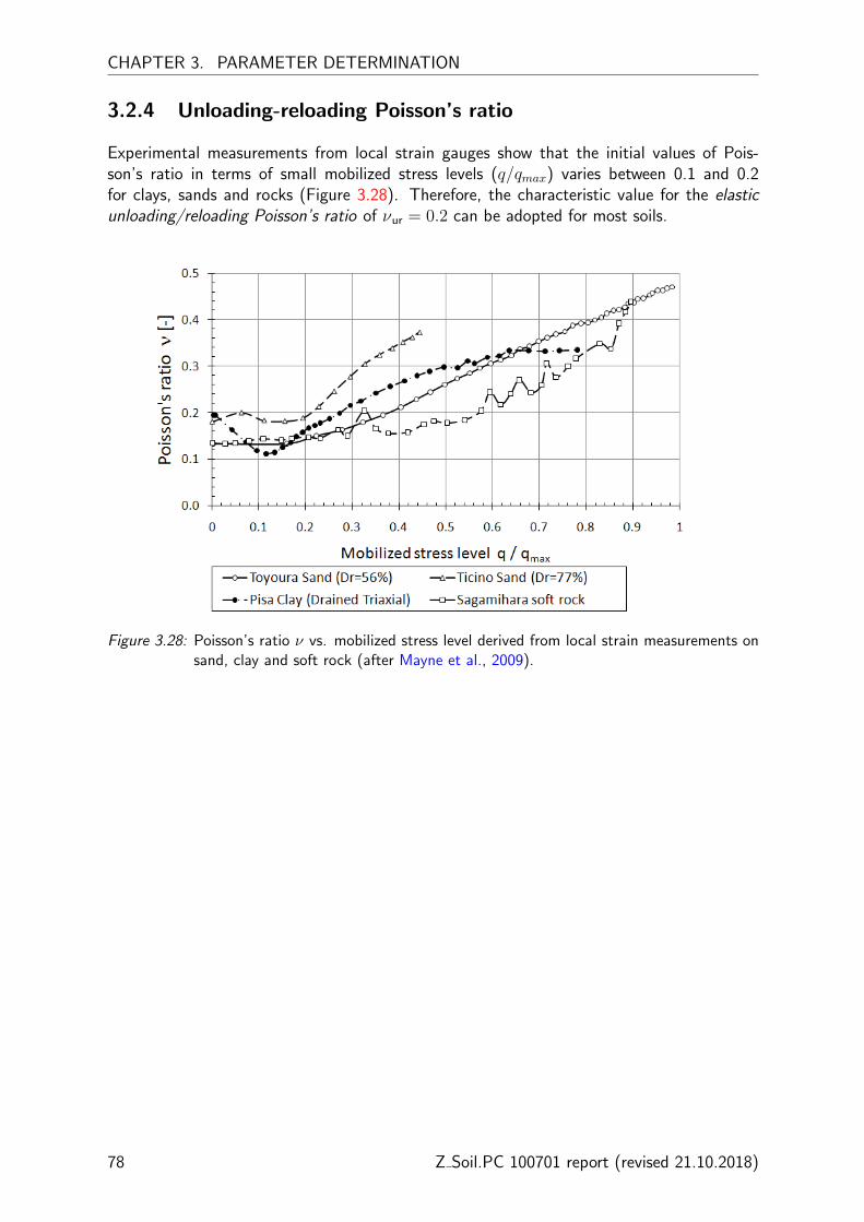
CHAPTER 3. PARAMETER DETERMINATION
3.2.4 Unloading-reloading Poisson’s ratio
Experimental measurements from local strain gauges show that the initial values of Pois-son’s ratio in terms of small mobilized stress levels (q/qmax) varies between 0.1 and 0.2for clays, sands and rocks (Figure 3.28). Therefore, the characteristic value for the elasticunloading/reloading Poisson’s ratio of νur = 0.2 can be adopted for most soils.
Figure 3.28: Poisson’s ratio ν vs. mobilized stress level derived from local strain measurements onsand, clay and soft rock (after Mayne et al., 2009).
78 Z Soil.PC 100701 report (revised 21.10.2018)
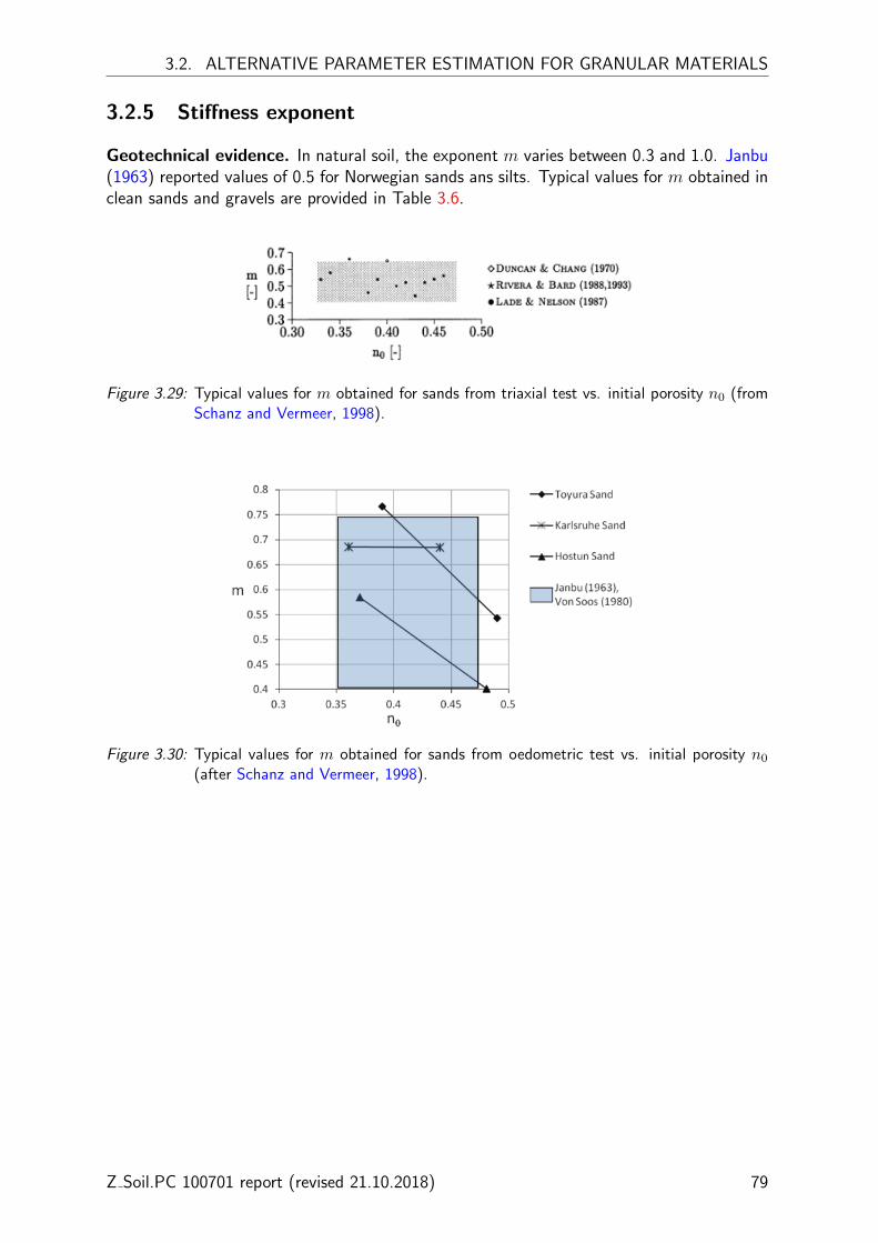
3.2. ALTERNATIVE PARAMETER ESTIMATION FOR GRANULAR MATERIALS
3.2.5 Stiffness exponent
Geotechnical evidence. In natural soil, the exponent m varies between 0.3 and 1.0. Janbu(1963) reported values of 0.5 for Norwegian sands ans silts. Typical values for m obtained inclean sands and gravels are provided in Table 3.6.
Figure 3.29: Typical values for m obtained for sands from triaxial test vs. initial porosity n0 (fromSchanz and Vermeer, 1998).
Figure 3.30: Typical values for m obtained for sands from oedometric test vs. initial porosity n0(after Schanz and Vermeer, 1998).
Z Soil.PC 100701 report (revised 21.10.2018) 79

CHAPTER 3. PARAMETER DETERMINATION
Table 3.6: Typical values for m observed in clean sands and gravels for the shear modulus G0 (fromBenz, 2007).
Soil tested m [-] Reference
Kenya carbonate sand 0.45-0.52 Fioravante (2000)Quiou carbonate sand 0.62 Lo Presti et al. (1993)Ottawa sand No.20-30 0.50 Hardin and Richart Jr (1963)SLB sand (subround) 0.44-0.53 Hoque and Tatsuoka (2004)Toyoura sand (subangular) 0.41-0.51 Hoque and Tatsuoka (2004)Toyoura sand (subangular) 0.50-0.57 Chaudary et al. (2004)Toyoura sand (subangular) 0.45 Lo Presti et al. (1993)Ticino sand (subangular) 0.44-0.53 Hoque and Tatsuoka (2004)Ticino sand (subangular) 0.43 Lo Presti and Jamiolkowski (1998)Ticino sand (subangular) 0.43-0.48 Fioravante (2000)H.River sand (subangular) 0.5-0.52 Kuwano and Jardine (2002)Silica sand (subangular) 0.5 Kallioglou et al. (2003)Hostun sand (angular) 0.47 Hoque and Tatsuoka (2000)Silica sand (angular) 0.50 Kallioglou et al. (2003)Silica sand 0.42 Wichtmann and Triantafyllidis (2004)Hime gravel (subround) 0.45-0.51 Chaudary et al. (2004)Chiba gravel (subround) 0.50 Modoni et al. (1999)
Table 3.7: Suggested ranges of stiffness exponent m observed for oedometric modulus Eoed (vonSoos, 1991).
Soil type m [-]
Gravel: poorly-graded (uniform) 0.4÷ 0.6Gravel: sandy, well-graded 0.5÷ 0.7Gravel: silty or clayey, well-graded, not crushed 0.5÷ 0.7Gravel-sand-clay mixture, crushed 0.7÷ 0.9Sand: fine, uniform 0.6÷ 0.75Sand: coarse, uniform 0.55÷ 0.7Sand: well-graded and gravelly sand 0.55÷ 0.7Sand: with fines, not crushed 0.65÷ 0.8Sand: with fines, crushed 0.75÷ 0.9
80 Z Soil.PC 100701 report (revised 21.10.2018)
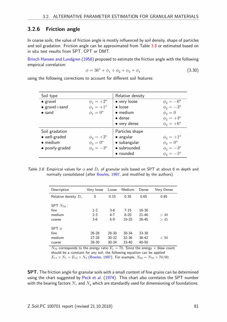
3.2. ALTERNATIVE PARAMETER ESTIMATION FOR GRANULAR MATERIALS
3.2.6 Friction angle
In coarse soils, the value of friction angle is mostly influenced by soil density, shape of particlesand soil gradation. Friction angle can be approximated from Table 3.8 or estimated based onin situ test results from SPT, CPT or DMT.
Brinch Hansen and Lundgren (1958) proposed to estimate the friction angle with the followingempirical correlation:
φ = 36o + φ1 + φ2 + φ3 + φ4 (3.30)
using the following corrections to account for different soil features:
Soil type Relative density• gravel φ1 = +2o • very loose φ2 = −6o
• gravel+sand φ1 = +1o • loose φ2 = −3o
• sand φ1 = 0o • medium φ2 = 0• dense φ2 = +3o
• very dense φ2 = +6o
Soil gradation Particles shape• well-graded φ3 = +3o • angular φ2 = +1o
• medium φ3 = 0o • subangular φ2 = 0o
• poorly-graded φ3 = −3o • subrounded φ2 = −3o
• rounded φ2 = −5o
Table 3.8: Empirical values for φ and Dr of granular soils based on SPT at about 6 m depth andnormally consolidated (after Bowles, 1997, and modified by the authors).
Description Very loose Loose Medium Dense Very Dense
Relative density Dr 0 0.15 0.35 0.65 0.85
SPT N70 :fine 1-2 3-6 7-15 16-30medium 2-3 4-7 8-20 21-40 > 40coarse 3-6 5-9 10-25 26-45 > 45
SPT φfine 26-28 28-30 30-34 33-38medium 27-28 30-32 32-36 36-42 < 50coarse 28-30 30-34 33-40 40-50
N70 corresponds to the energy ratio Er = 70. Since the energy × blow countshould be a constant for any soil, the following equation can be appliedEr1 ×N1 = Er2 ×N2 (Bowles, 1997). For example, N60 = N70 × 70/60.
SPT. The friction angle for granular soils with a small content of fine grains can be determinedusing the chart suggested by Peck et al. (1974). This chart also correlates the SPT numberwith the bearing factors Nγ and Nq which are standardly used for dimensioning of foundations.
Z Soil.PC 100701 report (revised 21.10.2018) 81

CHAPTER 3. PARAMETER DETERMINATION
Soil densityDense Very denseCompactL
oos
e
Ver
ylo
ose
Bea
ring
fact
orsNγ,Nq
Num
ber
ofbl
ows
per
30cm
Friction angle [o]
Figure 3.31: Determination of the friction angle φ′ and bearing factors for granular soils based onthe SPT number (from Peck et al., 1974).
Table 3.9: Estimation of the friction angle φ′ from the SPT number.
Standard Penetration Resistance Friction angle, φ [o]
Soil type N60, blows/0.3m Peck et al. (1974) Meyerhof (1956)
Very loose sand < 4 < 29 < 30Loose sand 4-10 29-30 30-35Medium sand 10-30 30-36 35-40Dense sand 30-50 36-41 40-45Very dense sand > 50 > 41 > 45
82 Z Soil.PC 100701 report (revised 21.10.2018)

3.2. ALTERNATIVE PARAMETER ESTIMATION FOR GRANULAR MATERIALS
Table 3.10: Empirical correlations relating SPT N -value with the effective friction angle for sands.
Empirical formula Reference Remarks
φ′peak =√
15.4N1,60 + 20oHatanaka and Uchida (1996)
tends to overestimate φ′ invery dense sands σ′v0 <100kPa
φ′peak =√
15.4N60 + 20o(±3o)Hatanaka and Uchida (1996) with-out overburden correction
simplification: σ′v0 = pa
φ′ =√
20N1,60 + 15oTeixeira (1996)
tends to overestimate φ′ invery dense sands σ′v0 <100kPa
φ′ = tan−1
N60
12.2 + 20.3σ′v0pa
0.34
Schmertmann (1975)tends to overestimate φ′ invery dense sands σ′v0 <100kPa
φ′ = tan−1(N60
32.5
)0.34
Schmertmann (1975) withoutoverburden correction
simplification: σ′v0 = pa
φ′ = 25o + 28
√N55
σ′v0after Townsend et al. (2003) tends to overestimate φ′ in
very dense sands σ′v0 <100kPa
φ′ = 15o +√
18N70Shioi and Fukui (1982)
Japan Road Associationstandards
φ′ = 27o + 0.36N70Shioi and Fukui (1982)
Japanese National Railwaystandards
N60 corresponds to the energy ratio Er = 60. Since the energy × blow countshould be a constant for any soil, the following equation can be appliedEr1 ×N1 = Er2 ×N2 (Bowles, 1997). For example, N55 = N60 × 60/55.
N1,60 = N60CN (”overburden-corrected” N60-value)
with the overburden correction factor CN = (pa/σ′v0)
0.5(Liao and Whitman, 1986)
use CN = 1.7 if CN > 1.7pa - atmospheric pressure (average sea-level pressure is 101.325 kPa)
Z Soil.PC 100701 report (revised 21.10.2018) 83
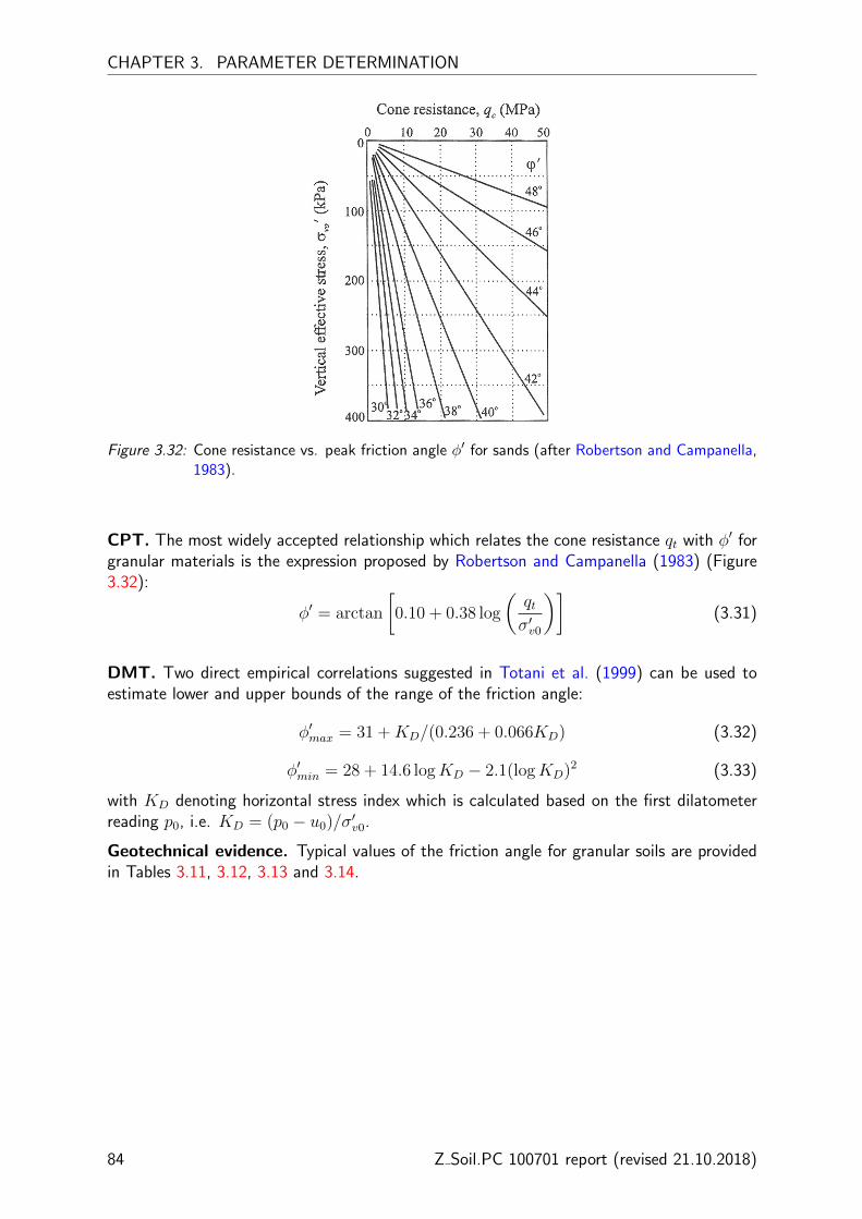
CHAPTER 3. PARAMETER DETERMINATION
Figure 3.32: Cone resistance vs. peak friction angle φ′ for sands (after Robertson and Campanella,1983).
CPT. The most widely accepted relationship which relates the cone resistance qt with φ′ forgranular materials is the expression proposed by Robertson and Campanella (1983) (Figure3.32):
φ′ = arctan
[0.10 + 0.38 log
(qtσ′v0
)](3.31)
DMT. Two direct empirical correlations suggested in Totani et al. (1999) can be used toestimate lower and upper bounds of the range of the friction angle:
φ′max = 31 +KD/(0.236 + 0.066KD) (3.32)
φ′min = 28 + 14.6 logKD − 2.1(logKD)2 (3.33)
with KD denoting horizontal stress index which is calculated based on the first dilatometerreading p0, i.e. KD = (p0 − u0)/σ′v0.
Geotechnical evidence. Typical values of the friction angle for granular soils are providedin Tables 3.11, 3.12, 3.13 and 3.14.
84 Z Soil.PC 100701 report (revised 21.10.2018)
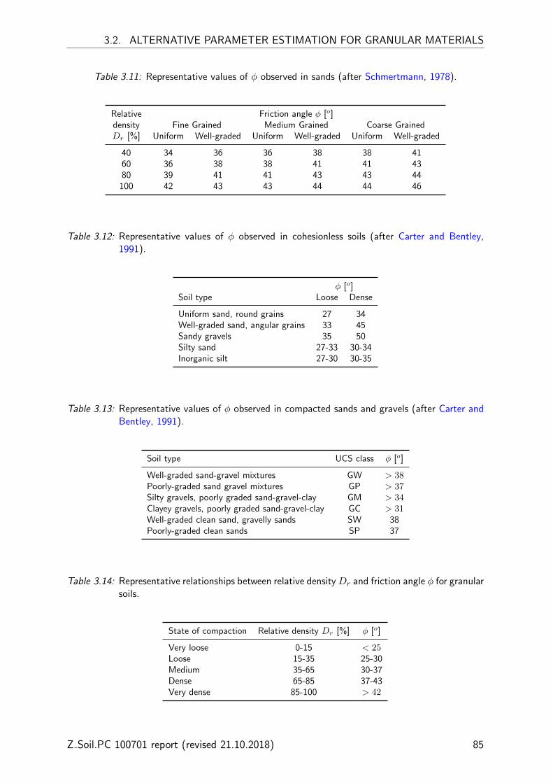
3.2. ALTERNATIVE PARAMETER ESTIMATION FOR GRANULAR MATERIALS
Table 3.11: Representative values of φ observed in sands (after Schmertmann, 1978).
Relative Friction angle φ [o]density Fine Grained Medium Grained Coarse GrainedDr [%] Uniform Well-graded Uniform Well-graded Uniform Well-graded
40 34 36 36 38 38 4160 36 38 38 41 41 4380 39 41 41 43 43 44
100 42 43 43 44 44 46
Table 3.12: Representative values of φ observed in cohesionless soils (after Carter and Bentley,1991).
φ [o]Soil type Loose Dense
Uniform sand, round grains 27 34Well-graded sand, angular grains 33 45Sandy gravels 35 50Silty sand 27-33 30-34Inorganic silt 27-30 30-35
Table 3.13: Representative values of φ observed in compacted sands and gravels (after Carter andBentley, 1991).
Soil type UCS class φ [o]
Well-graded sand-gravel mixtures GW > 38Poorly-graded sand gravel mixtures GP > 37Silty gravels, poorly graded sand-gravel-clay GM > 34Clayey gravels, poorly graded sand-gravel-clay GC > 31Well-graded clean sand, gravelly sands SW 38Poorly-graded clean sands SP 37
Table 3.14: Representative relationships between relative density Dr and friction angle φ for granularsoils.
State of compaction Relative density Dr [%] φ [o]
Very loose 0-15 < 25Loose 15-35 25-30Medium 35-65 30-37Dense 65-85 37-43Very dense 85-100 > 42
Z Soil.PC 100701 report (revised 21.10.2018) 85
CHAPTER 3. PARAMETER DETERMINATION
3.2.7 Dilatancy angle
It is typically observed in laboratory tests that for a very dense sand the value of the dilatancyangle ψ is about 1/3 of the peak friction angle φ′. In the case of loose sands, the dilatancyangle reduces to a few degrees, where as normally consolidated clays may exhibit no dilatancyat all. For example, Bolton (1986) reports ψmax = 14.7o for a dense sand which correspondedto the peak friction angle φ′max = 44.8o derived from a drained, plane strain compression test.
Bolton (1986) proposed that for well-compacted granular soils, the maximal dilatancy anglecan be estimated from:
ψ = 3.75IR under triaxial conditions (3.34a)
ψ = 6.25IR under plain strain conditions (3.34b)
with the relative dilatancy index IR can be estimated for well-compacted granular soils from:
IR = 5Dr − 1 (0 < IR < 4) (3.35)
with Dr denoting the relative density index
(=
emax − eemax − emin
).
Another reasonable approximation of ψ can be obtained using the following equation:
ψ = φ− 30o (3.36)
for the values of friction angle larger than 30o.Notice that the above approximation gives ψ ≈ φ′/3 for a dense gravel, whereas small valuesof ψ will be obtained for the the friction angles that correspond to loose sands (typicallyφ ≈ 30o to 32o).
86 Z Soil.PC 100701 report (revised 21.10.2018)

3.2. ALTERNATIVE PARAMETER ESTIMATION FOR GRANULAR MATERIALS
3.2.8 Coefficient of earth pressure ”at rest”
Various relationships can be found in literature for estimation of the coefficient of earthpressure ”at rest” for normally consolidated soils. They commonly relate the value of KNC
0
to the effective friction angle φ′, and the most popular are6:
KNC0 = 1− sinφ′ (3.37a)
KNC0 = (
√2− sinφ′)/(
√2 + sinφ′) (Simpson, 1992) (3.37b)
These equations are illustrated in Fig.3.33.
Figure 3.33: Typical relationships between KNC0 and φ′ observed for soils.
In the case of sands, the notion of preconsolidation pressure is not as meaningful as for co-hesive soils, and therefore OCR = 1 (i.e. KSR
0 = KNC0 ) can be assumed when calculating
parameters H and M .
In the case of running a simulation of isotropic consolidation (the case of isotropicallyconsolidated triaxial compression tests, i.e. CIU or CID), the coefficient should be assumedas KSR
0 = 1.
6Note that Eq.(3.37a) is often erroneously called ”Jaky’s equation” as it is a simplified form of his originalexpression KNC
0 = (1 − sinφ′)/(1 + sinφ′)(1 + 2/3 sinφ′) (Jaky, 1947) which gives essentially the sameresults as Eq.(3.87).
Z Soil.PC 100701 report (revised 21.10.2018) 87

CHAPTER 3. PARAMETER DETERMINATION
3.2.9 Void ratio
Void ratio for a saturated soil can be calculated from:
e = wnGs (3.38)
where wn is the water content, Gs is the specific gravity of soil solids and S is the saturationratio.In the case of partially unsaturated soil, the void ratio can be obtained from:
γ =Gsγw(1 + wn)
1 + eor e =
Gsγwγd− 1 or e = wnGs/S (3.39)
where γd is the dry unit weight.Hence, the maximum void ratio emax can be calculated from:
emax =Gsγwγd,min
− 1 (3.40)
The maximum void ratio emax can also be estimated according to approximate relationshippresented in Figure 3.34 between the void ratio the coefficient of uniformity for differentgranular soils.Typical values of void ratios and dry unit weights observed in granular soils are provided in
Table 3.15.
Table 3.15: Typical values of void ratio and dry unit weights observed in granular soils (after Das,2008).
Voids ratio Dry unit weighte [–] γ [kN/m3]
Soil type Max Min Min Max
Gravel 0.6 0.3 16 20Coarse sand 0.75 0.35 15 19Fine sand 0.85 0.4 14 19Standard Ottawa sand 0.8 0.5 14 17Gravelly sand 0.7 0.2 15 22Silty sand 1 0.4 13 19Silty sand and gravel 0.85 0.15 14 23
88 Z Soil.PC 100701 report (revised 21.10.2018)

3.2. ALTERNATIVE PARAMETER ESTIMATION FOR GRANULAR MATERIALS
Figure 3.34: Generalized charts for estimating emax, and emin from gradational and particle shapecharacteristics (from UFC, 2004; Das, 2008).
Z Soil.PC 100701 report (revised 21.10.2018) 89

CHAPTER 3. PARAMETER DETERMINATION
3.2.10 Overconsolidation ratio
CPT. Estimation of OCR from CPT data in sands can be carried out using a relationshipdeveloped based on statistical multiple regression analysis of 26 separate sands worldwide withflexible-walled calibration chambers (Kulhawy and Mayne, 1990; Lunne et al., 1997; Mayneet al., 2001; Mayne, 2007). Primarily clean siliceous (quartz and feldspar) sand samples wheresubject to normally-consolidated and overconsolidated states 1 ≤ OCR ≤ 15. Sands in thetest were usually dry or saturated without back pressures. The obtained empirical equationis the following:
OCR =
0.192
(qtpa
)0.22
(1− sinφ′)
(σ′v0pa
)0.31
1
sinφ′ − 0.27
(3.41)
with qt denoting cone tip resistance, σ′v0 effective overburden stress, and atmospheric pressureis pa = 100 kPa.
90 Z Soil.PC 100701 report (revised 21.10.2018)

3.2. ALTERNATIVE PARAMETER ESTIMATION FOR GRANULAR MATERIALS
3.2.11 Coefficient of earth pressure ”at rest”
CPT. Estimation of K0 from CPT data in sands can be carried out using a relationshipdeveloped based on statistical multiple regression analysis of 26 separate sands worldwide withflexible-walled calibration chambers (Kulhawy and Mayne, 1990; Lunne et al., 1997; Mayneet al., 2001; Mayne, 2007). Primarily clean siliceous (quartz and feldspar) sand samples wheresubject to normally-consolidated and overconsolidated states 1 ≤ OCR ≤ 15. Sands in thetest were usually dry or saturated without back pressures. The obtained empirical equationis the following:
K0 = 0.192
(qtpa
)0.22(paσ′v0
)0.31
OCR0.27 (3.42)
with qt denoting cone tip resistance, OCR overconsolidation ratio, and atmospheric pressureis pa = 100 kPa.
DMT-CPT. In 1980’s, researchers reported that a unique correlation for K0 from KD cannotbe established for sands as data points showed that such correlation in sand also dependson φ or Dr. Initially developed Marchetti’s chart K0 − qc − KD (Marchetti, 1985) wasupdated by Baldi et al. (1986) by incorporating all subsequent calibration chamber researchand converted into a simple algebraic equations:
K0 = 0.376 + 0.095KD − 0.0017qc/σ′v0 for ”freshly” deposited sand (3.43a)
K0 = 0.376 + 0.095KD − 0.0046qc/σv0 for ”seasoned” sand) (3.43b)
Marchetti et al. (2001) recommend to use Eq.(3.43a) in ”freshly deposited” sand, whereasfor ”seasoned” sands Eq.(3.43b).
Z Soil.PC 100701 report (revised 21.10.2018) 91

CHAPTER 3. PARAMETER DETERMINATION
3.3 Alternative parameter estimation for cohesive materials
3.3.1 Initial stiffness modulus and small strain threshold
The present section provides a number of approaches for estimating the initial soil stiffnessand the small strain threshold γ0.7. Some correlations allows to directly approximate theinput parameter E0, the others provide solutions for estimating the initial shear modulus G0.Then the input parameter E0 can be obtained through:
E0 = 2(1 + νur)G0 (3.44)
assuming a constant value of the unloading-reloading Poisson’s coefficient νur.
Geotechnical evidence. Experimental data shows that the initial stiffness of soils maydepend on the stress level, soil porosity and overconsolidation. These factors can be takeninto account using a modified equation proposed by Hardin and Black (1969):
G0 = A · f(e) ·OCRk
(p′
pref
)m, in [MPa] (3.45)
where G0 is the maximum small-strain shear modulus in MPa, p′ is the mean effective stressin kPa, pref is the reference stress equal to the atmospheric pressure pref = 100 kPa, OCRis the overconsolidation ratio and A, f(e), k, m are the correlated functions and parameterswhich are given in Table 3.16 and 3.18 for different types of soils. It is observed that theempirical exponent k varies from 0 for sands and 0.5 for high plasticity clays. It means thatk may increase with soil plasticity and its value can be taken from Table 3.17.
Biarez and Hicher (1994) proposed a simple relationship for all soils with wL < 50%:
E0 =140
e
(p′
pref
)0.5
, in [MPa] (3.46)
92 Z Soil.PC 100701 report (revised 21.10.2018)

3.3. ALTERNATIVE PARAMETER ESTIMATION FOR COHESIVE MATERIALS
Table 3.16: Parameters for estimation of G0 in clays using Eq.(3.45).
Soil tested IP A f(e) k mp Reference[%] [-] [-] [-] [-]
Quaternary Italianclays (see Fig.3.35)
- 60 e−1.30 N/A 0.50 Jamiolkowski et al. (1995)
Avezzano clay(Holocene-Pleistocene)
10-30 74 e−1.27 N/A 0.46 Lo Presti and Jamiolkowski (1998)
Fucino clay(Holocene-Pleistocene)
45-75 64 e−1.52 N/A 0.40 Lo Presti and Jamiolkowski (1998)
Garigliano clay(Holocene)
10-40 44 e−1.11 N/A 0.58 Lo Presti and Jamiolkowski (1998)
Panigaglia clay(Holocene)
44 44 e−1.30 N/A 0.50 Lo Presti and Jamiolkowski (1998)
Montaldo di Castroclay (Pleistocene)
15-34 50 e−1.33 N/A 0.40 Lo Presti and Jamiolkowski (1998)
ReconstitutedValericca clay(Pleistocene)
27 44 1 N/A 0.85 Rampello et al. (1997)
Pisa clay (Pleis-tocene)
23-46 50 e−1.43 N/A 0.44 Lo Presti and Jamiolkowski (1998)
London clay (recon-stituted)
41 13 1 0.25∗ 0.76 Viggiani and Atkinson (1995)
Speswhite kaolinclay (reconstituted)
24 40 1 0.2∗ 0.65 Viggiani and Atkinson (1995)
Kaolin clay 35 45(2.97− e)2
1 + eN/A 0.50 Marcuson and Wahls (1972)
Bentonite clay 60 4.5(4.40− e)2
1 + eN/A 0.50 Marcuson and Wahls (1972)
∗overconsolidation ratio OCR based on the mean stress (OCR = p′c/p′)
Table 3.17: Overconsolidation ratio exponent k used in Eq.(3.45).
Plasticity Index ExponentIP [%] k [-]
0 0.0020 0.1840 0.3060 0.4180 0.48
≥ 100 0.50
source: Kramer (1996, after Hardin&Drnevich 1972)
Z Soil.PC 100701 report (revised 21.10.2018) 93
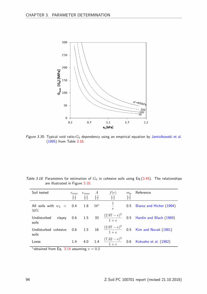
CHAPTER 3. PARAMETER DETERMINATION
Figure 3.35: Typical void ratio-G0 dependency using an empirical equation by Jamiolkowski et al.(1995) from Table 3.16.
Table 3.18: Parameters for estimation of G0 in cohesive soils using Eq.(3.45). The relationshipsare illustrated in Figure 3.10.
Soil tested emin emax A f(e) mp Reference[-] [-] [-] [-] [-]
All soils with wL <50%
0.4 1.8 58∗1
e0.5 Biarez and Hicher (1994)
Undisturbed clayeysoils
0.6 1.5 33(2.97− e)2
1 + e0.5 Hardin and Black (1969)
Undisturbed cohesivesoils
0.6 1.5 16(2.97− e)2
1 + e0.5 Kim and Novak (1981)
Loess 1.4 4.0 1.4(7.32− e)2
1 + e0.6 Kokusho et al. (1982)
∗obtained from Eq. 3.14 assuming ν = 0.2
94 Z Soil.PC 100701 report (revised 21.10.2018)

3.3. ALTERNATIVE PARAMETER ESTIMATION FOR COHESIVE MATERIALS
Geotechnical evidence. In case of lack of test data at very small strains, E0 for cohesivesoils can be evaluated from an empirical relation proposed by Alpan (1970), see Figure 3.11.The chart relates so-called ”static” modulus Es to the ”dynamic” modulus Ed. For the sakeof HS-SmallStrain model, Es can be considered as Eur obtained at engineering strain levels(ε ≈ 10−3), whereas E0 can be considered as ≈ Ed.
Geotechnical evidence. It can be observed in laboratory test that secant stiffness reduceswith mobilization of the shear strength. Mayne (2007) provides a selection of secant moduluscurves, represented by the ratio Gs/G0 or Es/E0. The collected results were derived frommonotonic laboratory shear tests performed on an sorted mix of clayey ans sandy materials,and they are presented in Figure 3.13.Geotechnical evidence and authors’ experience show that E0/E50 ratio varies in naturalclays from 4.6 to 30 depending on soil aging and particle bonding. The higher values ofE0/E50 ratio are suggested for aged, cemented and structured clay, whereas the lower onesfor insensitive, unstructured and remoulded clays.
CPT. A relationship between G0 and corrected tip resistance qt for clays has been proposedby Mayne and Rix (1993). The correlation also depends upon the inplace void ratio e0 (cf.Figure 3.36):
G0 = 49.4q0.695t e−1.130 in MPa (3.47)
with qt in [MPa].The effective vertical stress σ′v0 can used to recalculate the estimated modulus E0 = 2G0(1+νur) to the reference one Eref
0 using the stiffness dependency power law assuming that minorstress σ3 equal to min (σ′v0;σ
′v0 ·K0).
CPT. Based on a database for ten Norwegian marine soft clay sites, Long and Shane (2010)proposed an expression obtained by modifying the original expression by Simonini and Cola(2000). The relationship, apart of qt, also accounts for pore pressure measurements (cf.Figure 3.36). The modification was related to replacing ∆u/qc ratio with pore pressureparameter Bq (= (u2 − u0)/(qt − σv0)) and tunning empirical coefficients.
G0 = 4.39q1.225t (1 +Bq)2.53 ±50% (3.48)
with G0, qt in kPa and Bq is a dimensionless pore pressure parameter.
DMT. G0 can be estimated based on DMT data using a correlation reported by Hryciw(1990). The correlation was originally proposed for sands, silts and clays, however it seemsto underestimate G0 in sands (cf. Figure 3.37):
G0 =530
(σ′v0/pa)0.25
γDMT/γW − 1
2.7− γDMT/γW
K0.250 (paσ
′v0)
0.5(3.49)
with G0, pa, σ′v0 in same units; γDMT/γW dilatomter-based unit weight ratio obtained usingMarchetti’s chart for soil type and unit weight estimation.
Z Soil.PC 100701 report (revised 21.10.2018) 95

CHAPTER 3. PARAMETER DETERMINATION
Figure 3.36: Comparison of empirical correlations for estimating G0 (Gmax) in clays from CPTdata; plot for Eq. (3.47) obtained for e0 = 0.8.
Figure 3.37: Estimating G0 from DMT data using Eq.(3.49) proposed by Hryciw (1990) (plotobtained for K0 = 0.5).
96 Z Soil.PC 100701 report (revised 21.10.2018)
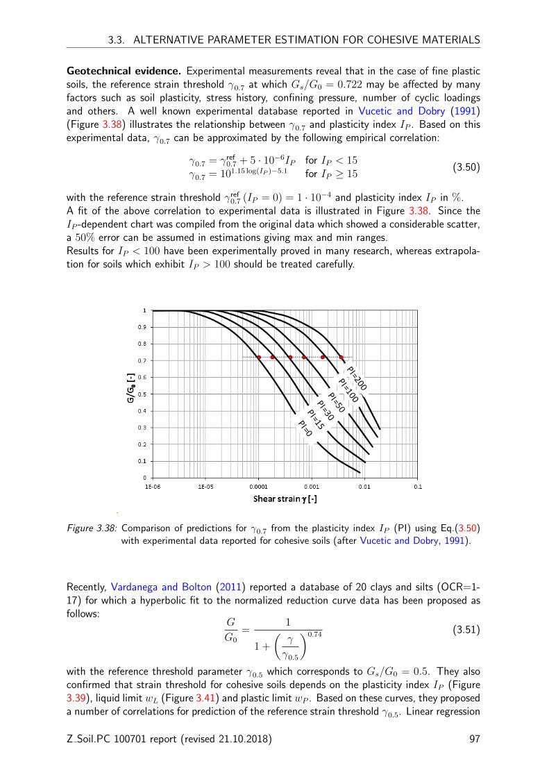
3.3. ALTERNATIVE PARAMETER ESTIMATION FOR COHESIVE MATERIALS
Geotechnical evidence. Experimental measurements reveal that in the case of fine plasticsoils, the reference strain threshold γ0.7 at which Gs/G0 = 0.722 may be affected by manyfactors such as soil plasticity, stress history, confining pressure, number of cyclic loadingsand others. A well known experimental database reported in Vucetic and Dobry (1991)(Figure 3.38) illustrates the relationship between γ0.7 and plasticity index IP . Based on thisexperimental data, γ0.7 can be approximated by the following empirical correlation:
γ0.7 = γref0.7 + 5 · 10−6IP for IP < 15
γ0.7 = 101.15 log(IP )−5.1 for IP ≥ 15(3.50)
with the reference strain threshold γref0.7 (IP = 0) = 1 · 10−4 and plasticity index IP in %.
A fit of the above correlation to experimental data is illustrated in Figure 3.38. Since theIP -dependent chart was compiled from the original data which showed a considerable scatter,a 50% error can be assumed in estimations giving max and min ranges.Results for IP < 100 have been experimentally proved in many research, whereas extrapola-tion for soils which exhibit IP > 100 should be treated carefully.
Figure 3.38: Comparison of predictions for γ0.7 from the plasticity index IP (PI) using Eq.(3.50)with experimental data reported for cohesive soils (after Vucetic and Dobry, 1991).
Recently, Vardanega and Bolton (2011) reported a database of 20 clays and silts (OCR=1-17) for which a hyperbolic fit to the normalized reduction curve data has been proposed asfollows:
G
G0
=1
1 +
(γ
γ0.5
)0.74 (3.51)
with the reference threshold parameter γ0.5 which corresponds to Gs/G0 = 0.5. They alsoconfirmed that strain threshold for cohesive soils depends on the plasticity index IP (Figure3.39), liquid limit wL (Figure 3.41) and plastic limit wP . Based on these curves, they proposeda number of correlations for prediction of the reference strain threshold γ0.5. Linear regression
Z Soil.PC 100701 report (revised 21.10.2018) 97

CHAPTER 3. PARAMETER DETERMINATION
analyzes were characterized by reasonable R2 values although an error band of ±50% wasobserved. For the purpose of this report, the original coefficients obtained through regressionanalyzes for γ0.5 where recalculated to the model parameter γ0.7:
γ0.7 =0.5975IP [−]
1000±50%, R2 = 0.75, n = 61, for IP = 10− 150% (3.52a)
γ0.7 =0.3442wL[−]
1000±50%, R2 = 0.75, n = 61, for wL = 25− 240% (3.52b)
γ0.7 =0.7517wP [−]
1000±50%, R2 = 0.57, n = 61, for wP = 12− 90% (3.52c)
Note that the above correlations account for no history stress nor confining pressure effects.
Figure 3.39: Comparison of predictions using Eq.(3.51) and (3.52a) with curves from Vucetic andDobry (1991).
98 Z Soil.PC 100701 report (revised 21.10.2018)
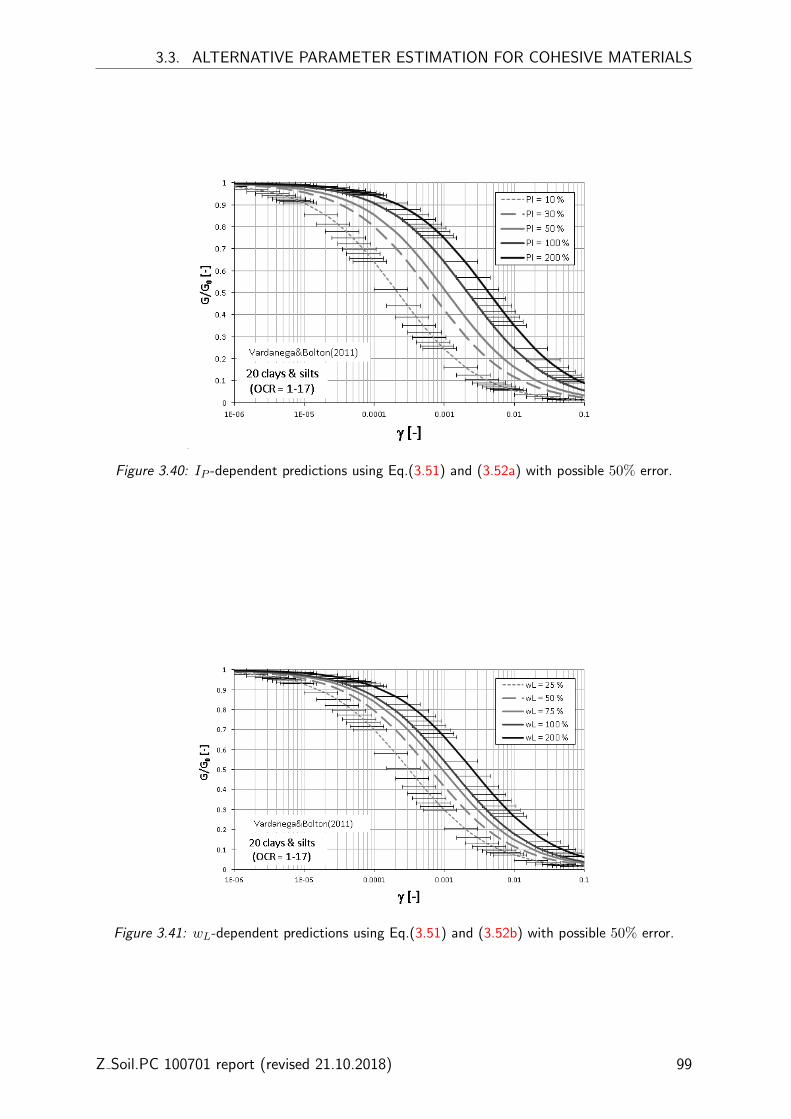
3.3. ALTERNATIVE PARAMETER ESTIMATION FOR COHESIVE MATERIALS
Figure 3.40: IP -dependent predictions using Eq.(3.51) and (3.52a) with possible 50% error.
Figure 3.41: wL-dependent predictions using Eq.(3.51) and (3.52b) with possible 50% error.
Z Soil.PC 100701 report (revised 21.10.2018) 99
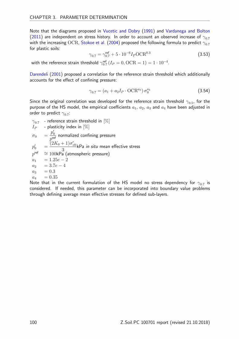
CHAPTER 3. PARAMETER DETERMINATION
Note that the diagrams proposed in Vucetic and Dobry (1991) and Vardanega and Bolton(2011) are independent on stress history. In order to account an observed increase of γ0.7with the increasing OCR, Stokoe et al. (2004) proposed the following formula to predict γ0.7for plastic soils:
γ0.7 = γref0.7 + 5 · 10−6IPOCR0.3 (3.53)
with the reference strain threshold γref0.7 (IP = 0,OCR = 1) = 1 · 10−4.
Darendeli (2001) proposed a correlation for the reference strain threshold which additionallyaccounts for the effect of confining pressure:
γ0.7 = (a1 + a2IP ·OCRa3)σa40 (3.54)
Since the original correlation was developed for the reference strain threshold γ0.5, for thepurpose of the HS model, the empirical coefficients a1, a2, a3 and a4 have been adjusted inorder to predict γ0.7:
γ0.7 - reference strain threshold in [%]IP - plasticity index in [%]
σ0 =p′0pref
normalized confining pressure
p′0 =(2K0 + 1)σ′v0
3kPa in situ mean effective stress
pref ∼= 100kPa (atmospheric pressure)a1 = 1.25e− 2a2 = 3.7e− 4a3 = 0.3a4 = 0.35
Note that in the current formulation of the HS model no stress dependency for γ0.7 isconsidered. If needed, this parameter can be incorporated into boundary value problemsthrough defining average mean effective stresses for defined sub-layers.
100 Z Soil.PC 100701 report (revised 21.10.2018)

3.3. ALTERNATIVE PARAMETER ESTIMATION FOR COHESIVE MATERIALS
6-
?
Figure 3.42: A graphical interpretation of Eq.(3.54): an example of estimation of shear strain thresh-old γ0.7 for IP = 40%, OCR = 4 and mean effective stress p′0 = 400kPa.
Z Soil.PC 100701 report (revised 21.10.2018) 101

CHAPTER 3. PARAMETER DETERMINATION
3.3.2 Strength parameters
It is commonly known that the strength of clays in terms of effective stresses is mostly fric-tional and the effective cohesion c′ ≈ 0. Small values of cohesion which are observed duringtesting may appear in partially saturated clays where the meniscus effects (suction) draw soilparticles together resulting in inter-particles stresses. Larger magnitudes of cohesion can beoften observed in cemented soils due to bonding effects.
Geotechnical evidence. The values of the effective friction angle φ′ observed for fine soilsfall in a wide range from 18o to 42o. Some representative values of φ′ for compacted claysare provided in Table 3.19 after Carter and Bentley (1991).
Table 3.19: Representative values of φ′ observed in compacted clays (after Carter and Bentley,1991).
Soil type UCS class φ [o]
Silty clays, sand-silt mix SM 34Clayey sands, sandy-clay mix SC 31Silts and clayey silts ML 32Clays of low plasticity CL 28Clayey silts MH 25Clays of high plasticity CH 19
CPTU. The estimation of effective stress parameters from the total stress analysis of undrainedpenetration is difficult. The solution needs to account for excess pore water pressure for whichthe distribution around the cone is highly complex and difficult to model analytically. Inter-pretation methods can be thus viewed as rather approximative.The effective friction angle φ′ can be estimated using the solution which is based on thebearing capacity theory (Sandven et al., 1988)7:
qt − σvo = Nm(σ′vo + a) with Nm =Nq − 1
1 +NuBq(3.55)
where a′ denotes the attraction (a′ = c′ cotφ′), β is the angle of plastification, Nq and Nu
are the bearing capacity factors (Nq = Nq(φ′, β) and Nu
∼= Nu(φ)).Mayne (2005, 2007) proposed a simplified expression which is applicable to the ranges of20◦ ≤ φ′ ≤ 45◦ and 0.1 ≤ Bq ≤ 1.0 (see Figure 3.43). By setting for the above methodthe effective cohesion intercept c′ = 0 and plastification angle β = 0, the values of φ′ wereevaluated line-by-line and the following approximate expression was obtained:
φ′ ≈ 29.5◦B0.121q (0.256 + 0.336Bq + logQt) (3.56)
Strength parameters vs. undrained shear strength. Best-quality predictions of thestrength parameters φ′ and c′ for cohesive soils can be essentially derived from laboratorytests. In case of lack of laboratory data, these model parameters can be approximately cal-ibrated based on the undrained shear strength su. The magnitude of su can be determined
7The approach proposed by researchers from the Norwegian University of Science and Technology (NTNU)is referred to NTNU method.
102 Z Soil.PC 100701 report (revised 21.10.2018)
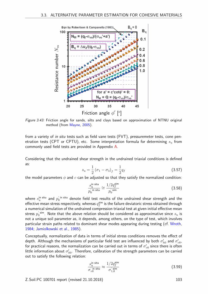
3.3. ALTERNATIVE PARAMETER ESTIMATION FOR COHESIVE MATERIALS
Friction angle φ′ [o]
Res
ista
nce
num
berNm
Figure 3.43: Friction angle for sands, silts and clays based on approximation of NTNU originalmethod (from Mayne, 2005).
from a variety of in situ tests such as field vane tests (FVT), pressuremeter tests, cone pen-etration tests (CPT or CPTU), etc. Some interpretation formula for determining su fromcommonly used field tests are provided in Appendix A.
Considering that the undrained shear strength in the undrained triaxial conditions is definedas:
su =1
2(σ1 − σ3)f =
1
2qf (3.57)
the model parameters φ and c can be adjusted so that they satisfy the normalized condition:
sin situu
p’ in situ0
∼=1/2qsim
f
p’ sim0
(3.58)
where sin situu and p’ in situ
0 denote field test results of the undrained shear strength and theeffective mean stress respectively, whereas qsim
f is the failure deviatoric stress obtained througha numerical simulation of the undrained compression triaxial test at given initial effective meanstress p’ sim
0 . Note that the above relation should be considered as approximative since su isnot a unique soil parameter as, it depends, among others, on the type of test, which involvesparticular strain paths related to dominant shear modes appearing during testing (cf. Wroth,1984; Jamiolkowski et al., 1985).
Conceptually, normalization of data in terms of initial stress conditions removes the effect ofdepth. Although the mechanisms of particular field test are influenced by both σ′h0 and σ′v0,for practical reasons, the normalization can be carried out in terms of σ′v0 since there is oftenlittle information about σ′h0. Therefore, calibration of the strength parameters can be carriedout to satisfy the following relation:
sin situu
σ’ in situv0
≈1/2qsim
f
σ’ sim1,0
(3.59)
Z Soil.PC 100701 report (revised 21.10.2018) 103

CHAPTER 3. PARAMETER DETERMINATION
where σ’ sim1,0 denotes the axial effective stress at the beginning of simulation.
The calibration procedure can be summarized as follows:
1. Assess field values of su for, at least, two different depths (different σ′v0) and plot the dataon σ′v0 − su chart.
2. Run two simulations of the undrained triaxial compression test (preferably aniotropically-consolidated with the specified KSR
0 6= 1.0) for different σ’ sim1,0 and corresponding OCRs
with an initial guess of parameters φ and c, and an assumed failure ratio Rf (note thatan explicit ultimate deviatoric stress can be obtained for the dilatancy angle ψ = 0, ornon-zero ψ with the assumed dilatancy cut-off).
3. Plot numerical results of 1/2qf on σ′v0− su chart (as in Figure 3.44) and check the degreeof fit for numerical and in situ trend lines.
4. Return to step 2 if the degree of fit is not satisfactory and modify parameters φ and c. Notethat each modification of φ and c requires updating KNC
0 and evaluating of parameters Mand H before the next calculation run.
Figure 3.44: Undrained shear strength su against normalizing effective stress σ’ sim1,0 (p∗ denotes the
intersection between deviatoric and isotropic mechanisms, see Figure ??).
In the case of overconsolidated material, if the initial mean effective stress p′0 lies before themean effective stress p∗ which value corresponds to the intersection between deviatoric andisotropic mechanisms (see Figure ??), qf can be estimated directly from the Mohr-Coulombcriterion (cf. Figure 3.1):
qf = α (p′0 + c cotφ) (3.60)
where α is related to the friction angle φ which depends on the dominating shear mode whichis appropriate to a given in situ test:
104 Z Soil.PC 100701 report (revised 21.10.2018)
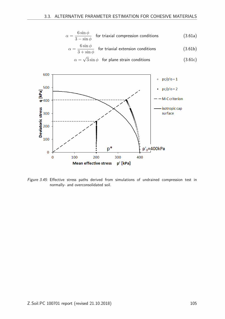
3.3. ALTERNATIVE PARAMETER ESTIMATION FOR COHESIVE MATERIALS
α =6 sinφ
3− sinφfor triaxial compression conditions (3.61a)
α =6 sinφ
3 + sinφfor triaxial extension conditions (3.61b)
α =√
3 sinφ for plane strain conditions (3.61c)
Figure 3.45: Effective stress paths derived from simulations of undrained compression test innormally- and overconsolidated soil.
Z Soil.PC 100701 report (revised 21.10.2018) 105

CHAPTER 3. PARAMETER DETERMINATION
3.3.3 Failure ratio
For most soils, the value of Rf falls between 0.75 and 1 and an average value of the failureratio can be taken as Rf = 0.9. Kempfert (2006) reported some Rf values derived fromtriaxial compression tests for three lacustrine soft soils in southern Germany:
• CICD test: Rf = 0.73− 0.88, with the average value of 0.82
• CICU test: Rf = 0.70− 0.99, with the average value of 0.89
106 Z Soil.PC 100701 report (revised 21.10.2018)

3.3. ALTERNATIVE PARAMETER ESTIMATION FOR COHESIVE MATERIALS
3.3.4 Dilatancy angle
While for granular soils the maximal dilatancy angle can be related to the relative density(Dr), an estimation of ψ for clays relies on geotechnical experience. For instance, it can beobserved in laboratory tests that normally consolidated clays may exhibit no dilatancy at all.Therefore, it is proposed that for cohesive soils, it can be assumed that dilatancy depends onthe preconsolidation state and ψ can be approximately taken as:
• ψ = 0o for normally- and ligthly-overconslidated soil
• ψ = φ′/6 for overconsolidated soil
• ψ = φ′/3 for heavily overconsolidated soil
Another reasonable approximation of ψ can be obtained using the following equation:
ψ = φ− 30o (3.62)
for the values of friction angle larger than 30o.Notice that the above approximation gives ψ ≈ φ′/3 for a dense gravel, whereas smallvalues of ψ will be obtained for the the friction angles that correspond to compacted silts orclays(typically φ ≈ 30o to 35o).
Z Soil.PC 100701 report (revised 21.10.2018) 107

CHAPTER 3. PARAMETER DETERMINATION
3.3.5 Stiffness moduli
In general, the relation between the stiffness moduli is as follows:
E50 < Es < Eur (3.63)
where Es denotes ”static” modulus or secant modulus taken from the initial part of the ε1−qexperimental curve at ε1 = 0.1%.
In the case when one of the stiffness moduli cannot be directly determined, it may be relevantfor many practical cases to set:
Erefur
Eref50
= 3 to 6 (an average can be assumed equal to 4) (3.64)
However, note that the following condition should be satisfied:Eref
ur
Eref50
> 2.
The secant modulus E50 can be approximated based on the known value of the ”static”modulus Es and according to the approach described in Section 3.2.2, Figure 3.22. A roughapproximation of the order of magnitudes for the ”static” modulus Es is given in Table 3.20.
Table 3.20: Typical values for the ”static” modulus Es [MPa] (compiled from Kezdi, 1974; Pratet al., 1995).
Soil Consistency
Very Soft Soft Medium Stiff Very Stiff Hard
Soil Type Min Max Min Max Min Max Min Max Min Max Min Max
Siltsslight plasticity 2.5 4 5 8 10 15 15 20 20 40 40 80low plasticity 1.5 3 3 6 6 10 10 15 15 30 30 60Clayslow to medium plast. 0.5 3 2 5 5 8 8 12 12 30 30 70high plasticity 0.35 2 1.5 4 4 7 7 12 12 20 20 32Silt organic 0.5 5Clay organic 0.5 4
Assuming that during unloading/reloading soil behaves elastically, the modulus Eur can berelated with the constrained unloading/reloading oedometric modulus Eoed,ur through:
Eur = Eoed,ur(1 + νur)(1− 2νur)
1− νur(3.65)
Note, however, that Eur is not a unique value for a given soil in the oedometric test becauseEur depends on the previous maximal stress level σ′c attained before the unloading and thecorresponding void ratio ec, as shown in Figure 3.46. Therefore, assuming an infinitesimalchange of the compression stress, i.e. ∆σ′ → 0, the unloading/reloading oedometric modulusEoed,ur should be approximated by similarity with Eq.(3.5) as:
Eoed,ur =2.3(1 + ec)
Csσ′c (3.66)
108 Z Soil.PC 100701 report (revised 21.10.2018)

3.3. ALTERNATIVE PARAMETER ESTIMATION FOR COHESIVE MATERIALS
where Cs is the swelling index (Figure 3.46).Since the Eoed,ur was approximated for the stress point belonging to the primary loading line(KNC
0 -line), such a determined reference unloading/reloading modulus Erefur corresponds thus
to the reference stress σref which can be estimated from:
σref = KNC0 σ′c (3.67)
Figure 3.46: Idealized plot of one-dimensional oedometric compression test.
DMT. The ”static” modulus corresponding to Eur can be evaluated for cohesive soils the ver-tical drained constrained modulus MDMT which is derived from three intermediate dilatometerparameters, i.e. the material index ID, the horizontal stress index KD, and the dilatometermodulus ED. Note that MDMT may correspond to Eref
oed only for normally-consolidated soil.The unloading-reloading modulus Eur can be evaluated assuming that:
Eur = Es = aEoed = aMDMT (3.68)
where a ≈ 0.9 as a = (1 + νur)(1 − 2νur)/(1 − νur) and the dilatometer vertical drainedconstrained modulus MDMT :
MDMT = RMED (3.69)
with ED = 34.7(p1 − p0) and RM depending on soil type behavior, i.e.
• clayey silt to sandy silt (0.6 < ID < 1.8): RM = RM,0 + (2.5−RM,0) logKD andRM,0 = 0.14 + 0.15(ID − 0.6)
• clay to silty clays (ID ≤ 0.6): RM = 0.14 + 2.36 logKD
• if KD > 10: RM = 0.32 + 2.18 logKD
• if RM < 0.85: set RM = 0.85
Undrained vs drained moduli - theoretical relationship. In case of lack of drainedcompression test data, the stiffness moduli can be calibrated based on the results derived fromthe undrained triaxial compression test (e.g. CIUC or CAUC). Since water filling skeleton
Z Soil.PC 100701 report (revised 21.10.2018) 109

CHAPTER 3. PARAMETER DETERMINATION
pores has no shear stiffness, the shear modulus is not affected by the drainage condition soone can write:
Eu
2(1 + νu)= Gu = G =
E
2(1 + ν)(3.70)
where νu is the Poisson’s coefficient in undrained conditions.Considering that the undrained conditions imply ε1 = ε3, and therefore νu = 0.5, the aboveequation can be rewritten as:
Eu
E=
3
2(1 + ν)(3.71)
and for the drained Poison’s coefficient ranging for most soils between 0.12 and 0.4:
Eu
E≈ 1.07 to 1.34 (3.72)
An assumption of νu = 0.5 for undrained conditions can also be expressed with the conditionof no volume change (∆εv = 0). Since the undrained bulk modulus Ku tends to infinity insuch conditions , νu → 0.5:
Ku =∆σ
∆εv=
Eu
3(1− 2νu)(3.73)
The undrained ”static” modulus Eus can be estimated based on a value of undrained shear
strength su using an empirical correlation:
Eu = Kcsu (3.74)
with an empirical correlation coefficient which depends on the plasticity index PI and OCR,and can be estimated from Figure 3.47.
Figure 3.47: Evaluating the undrained modulus from Eu from su: chart for estimating the correla-tion coefficient Kc in Eq. (3.74) (from Duncan and Buchignani, 1976).
110 Z Soil.PC 100701 report (revised 21.10.2018)

3.3. ALTERNATIVE PARAMETER ESTIMATION FOR COHESIVE MATERIALS
Undrained vs drained moduli - curve fitting. The ”drained” model moduli can alsobe calibrated by means of curve-fitting. It is recommended because in the ”undrained” testthe effective stress σ′3 (which corresponds to the reference stress) does not remain constantduring compression due to a development of excess pore water pressure. The calibration of”drained” stiffness moduli (E ′ur, E
′50) from ”undrained” test requires fitting laboratory data,
i.e. curve ε1 − q, with the results obtained through an axis-symmetric, one-element simula-tion of the undrained compression. The flowchart of the parameter calibration is presentedin detail in Figure 3.48 and it is described below.
Considering that strength parameters φ′ and c′ can be directly derived from undrained testdata, they should be kept unmodified during curve-fitting. In order to avoid excessive gainin material resistance after reaching the failure stress point, the dilatancy angle can be setψ = 0o during ”undrained” simulations (cf. Truty and Obrzud (2015)). The soil unit weightshould be set to γ = 0 in order to cancel body force loading. As regards the fluid weight theoption X Skip gravity term should be chosen. A non-zero value for the initial void ratio e0should be set.In order to represent the undrained behavior a finite value of the fluid bulk modulus shouldbe set, e.g. the bulk modulus of water is 2.2e6 kPa. The ratio between fluid and soil bulkmoduli should be of order Kf/K = 105 ÷ 106. It corresponds to the penalty formulationwhich may fail to converge if the penalty factor is too large. In such a case computation willbe terminated and some null pivots will be reported in the ∗.log file. In order to remedy sucha problem, the value of the fluid bulk modulus should be decreased. Note that the two-phasestabilization should not be activated in the single-element test as no pressure oscillation isobserved (pore pressure is constant over the element). No initial pressure BC need to beintroduced.The simulation should be carried out using Axisymmetry analysis type,Deformation+Flow problem type and Consolidation driver should be set for when runningcompression of the element.
Z Soil.PC 100701 report (revised 21.10.2018) 111

CHAPTER 3. PARAMETER DETERMINATION
Figure 3.48: Flowchart for calibration of stiffness moduli E0, Eur, E50 based on ε1−q curve derivedfrom the undrained compression triaxial test (CU) and a single-element test.
112 Z Soil.PC 100701 report (revised 21.10.2018)

3.3. ALTERNATIVE PARAMETER ESTIMATION FOR COHESIVE MATERIALS
Geotechnical evidence. Kempfert (2006) have provided typical results for the ratios be-tween stiffness moduli. These ratios are presented below in Tables 3.21 and 3.22.
Table 3.21: Relationship between triaxial stiffness moduli and oedometric moduli for three lacustrineclays in Germany, from Kempfert (2006).
Ei/Eoed E50/Eoed Eur/Eoed,ur Eoed,ur/Eoed
Soil 1 2.08 1.03 2.33-2.52 2.60Soil 2 1.63 0.77 1.29-2.09 3.63Soil 3 2.82 1.45 1.32-2.51 6.65
Average 2.17 1.08 4.29
Ei was derived from the initial slope of the triaxial curve ε1 − qEoed,ur denotes unloading/reloading oedometer modulus
Table 3.22: Relationship between stiffness moduli derived from drained and undrained triaxial testsfor three lacustrine clays in Germany, from Kempfert (2006).
Drainage conditions Ei/E50 Eur/Ei Eur/E50
Soil 1 drained 2.02 3.20 5.93undrained 1.48
Soil 2 drained 2.17 3.10 6.72undrained 1.84
Soil 3 drained 1.94 6.55 12.66undrained 3.02
Average drained 2.04 4.28 8.43undrained 2.11
Ei was derived from the initial slope of the triaxial curve ε1 − q
Z Soil.PC 100701 report (revised 21.10.2018) 113
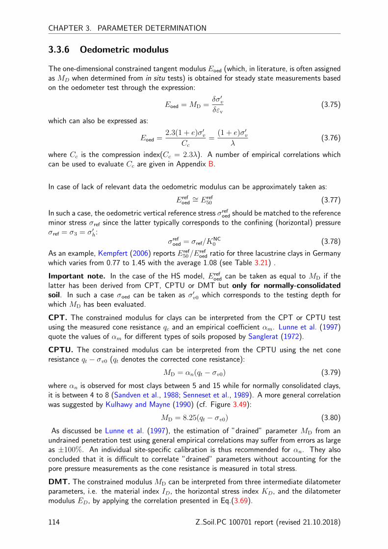
CHAPTER 3. PARAMETER DETERMINATION
3.3.6 Oedometric modulus
The one-dimensional constrained tangent modulus Eoed (which, in literature, is often assignedas MD when determined from in situ tests) is obtained for steady state measurements basedon the oedometer test through the expression:
Eoed = MD =δσ′vδεv
(3.75)
which can also be expressed as:
Eoed =2.3(1 + e)σ′v
Cc=
(1 + e)σ′vλ
(3.76)
where Cc is the compression index(Cc = 2.3λ). A number of empirical correlations whichcan be used to evaluate Cc are given in Appendix B.
In case of lack of relevant data the oedometric modulus can be approximately taken as:
Erefoed∼= Eref
50 (3.77)
In such a case, the oedometric vertical reference stress σrefoed should be matched to the reference
minor stress σref since the latter typically corresponds to the confining (horizontal) pressureσref = σ3 = σ′h:
σrefoed = σref/K
NC0 (3.78)
As an example, Kempfert (2006) reports Eref50 /E
refoed ratio for three lacustrine clays in Germany
which varies from 0.77 to 1.45 with the average 1.08 (see Table 3.21) .
Important note. In the case of the HS model, Erefoed can be taken as equal to MD if the
latter has been derived from CPT, CPTU or DMT but only for normally-consolidatedsoil. In such a case σoed can be taken as σ′v0 which corresponds to the testing depth forwhich MD has been evaluated.
CPT. The constrained modulus for clays can be interpreted from the CPT or CPTU testusing the measured cone resistance qc and an empirical coefficient αm. Lunne et al. (1997)quote the values of αm for different types of soils proposed by Sanglerat (1972).
CPTU. The constrained modulus can be interpreted from the CPTU using the net coneresistance qt − σv0 (qt denotes the corrected cone resistance):
MD = αn(qt − σv0) (3.79)
where αn is observed for most clays between 5 and 15 while for normally consolidated clays,it is between 4 to 8 (Sandven et al., 1988; Senneset et al., 1989). A more general correlationwas suggested by Kulhawy and Mayne (1990) (cf. Figure 3.49):
MD = 8.25(qt − σv0) (3.80)
As discussed be Lunne et al. (1997), the estimation of ”drained” parameter MD from anundrained penetration test using general empirical correlations may suffer from errors as largeas ±100%. An individual site-specific calibration is thus recommended for αn. They alsoconcluded that it is difficult to correlate ”drained” parameters without accounting for thepore pressure measurements as the cone resistance is measured in total stress.
DMT. The constrained modulus MD can be interpreted from three intermediate dilatometerparameters, i.e. the material index ID, the horizontal stress index KD, and the dilatometermodulus ED, by applying the correlation presented in Eq.(3.69).
114 Z Soil.PC 100701 report (revised 21.10.2018)
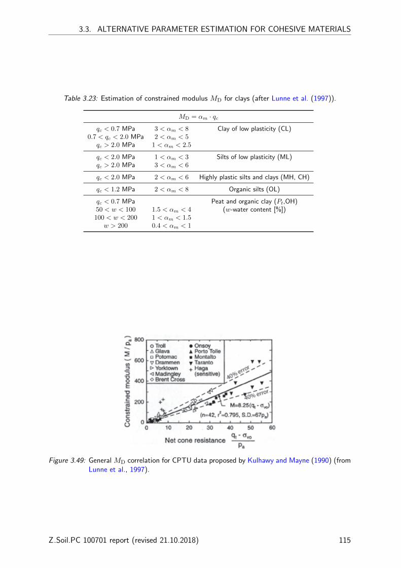
3.3. ALTERNATIVE PARAMETER ESTIMATION FOR COHESIVE MATERIALS
Table 3.23: Estimation of constrained modulus MD for clays (after Lunne et al. (1997)).
MD = αm · qcqc < 0.7 MPa 3 < αm < 8 Clay of low plasticity (CL)
0.7 < qc < 2.0 MPa 2 < αm < 5qc > 2.0 MPa 1 < αm < 2.5
qc < 2.0 MPa 1 < αm < 3 Silts of low plasticity (ML)qc > 2.0 MPa 3 < αm < 6
qc < 2.0 MPa 2 < αm < 6 Highly plastic silts and clays (MH, CH)
qc < 1.2 MPa 2 < αm < 8 Organic silts (OL)
qc < 0.7 MPa Peat and organic clay (Pt,OH)50 < w < 100 1.5 < αm < 4 (w-water content [%])100 < w < 200 1 < αm < 1.5
w > 200 0.4 < αm < 1
Figure 3.49: General MD correlation for CPTU data proposed by Kulhawy and Mayne (1990) (fromLunne et al., 1997).
Z Soil.PC 100701 report (revised 21.10.2018) 115
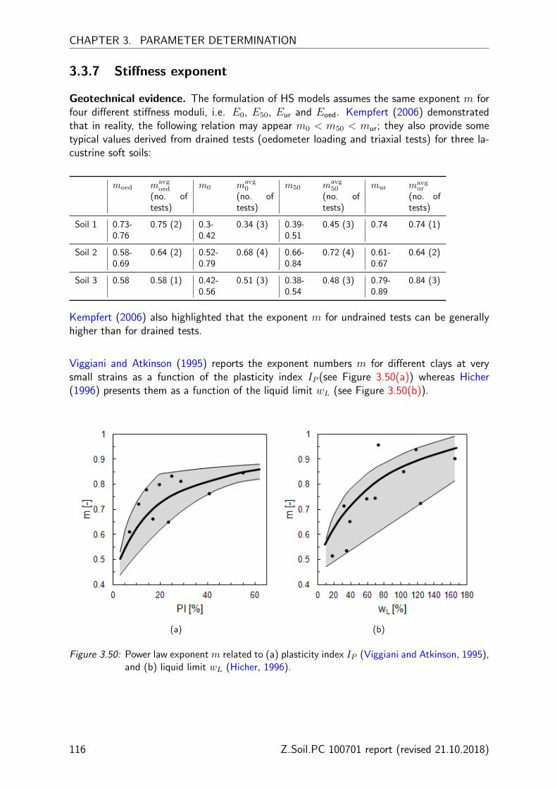
CHAPTER 3. PARAMETER DETERMINATION
3.3.7 Stiffness exponent
Geotechnical evidence. The formulation of HS models assumes the same exponent m forfour different stiffness moduli, i.e. E0, E50, Eur and Eoed. Kempfert (2006) demonstratedthat in reality, the following relation may appear m0 < m50 < mur; they also provide sometypical values derived from drained tests (oedometer loading and triaxial tests) for three la-custrine soft soils:
moed mavgoed m0 mavg
0 m50 mavg50 mur mavg
ur
(no. oftests)
(no. oftests)
(no. oftests)
(no. oftests)
Soil 1 0.73-0.76
0.75 (2) 0.3-0.42
0.34 (3) 0.39-0.51
0.45 (3) 0.74 0.74 (1)
Soil 2 0.58-0.69
0.64 (2) 0.52-0.79
0.68 (4) 0.66-0.84
0.72 (4) 0.61-0.67
0.64 (2)
Soil 3 0.58 0.58 (1) 0.42-0.56
0.51 (3) 0.38-0.54
0.48 (3) 0.79-0.89
0.84 (3)
Kempfert (2006) also highlighted that the exponent m for undrained tests can be generallyhigher than for drained tests.
Viggiani and Atkinson (1995) reports the exponent numbers m for different clays at verysmall strains as a function of the plasticity index IP (see Figure 3.50(a)) whereas Hicher(1996) presents them as a function of the liquid limit wL (see Figure 3.50(b)).
(a) (b)
Figure 3.50: Power law exponent m related to (a) plasticity index IP (Viggiani and Atkinson, 1995),and (b) liquid limit wL (Hicher, 1996).
116 Z Soil.PC 100701 report (revised 21.10.2018)

3.3. ALTERNATIVE PARAMETER ESTIMATION FOR COHESIVE MATERIALS
Table 3.24: Typical values for mp* observed in clays for the shear modulus G0 (from Benz, 2007).
Soil tested IP [%] mp [-] Reference
Avezzano clay (Holocene-Pleistocene) 10-30 0.46 Lo Presti and Jamiolkowski (1998)Fucino clay (Holocene-Pleistocene) 45-75 0.40 Lo Presti and Jamiolkowski (1998)Garigliano clay (Holocene) 10-40 0.58 Lo Presti and Jamiolkowski (1998)Panigaglia clay (Holocene) 44 0.50 Lo Presti and Jamiolkowski (1998)Montaldo di Castro clay (Pleistocene) 15-34 0.40 Lo Presti and Jamiolkowski (1998)Recon. Valericca clay (Pleistocene) 27 0.85 Rampello et al. (1997)Pisa clay (Pleistocene) 23-46 0.44 Lo Presti and Jamiolkowski (1998)London clay (reconstituted) 41 0.76 Viggiani and Atkinson (1995)Speswhite kaolin clay (reconstituted) 24 0.65 Viggiani and Atkinson (1995)Kaolin clay 35 0.50 Marcuson and Wahls (1972)Bentonite clay 60 0.50 Marcuson and Wahls (1972)
The number mp was obtained for the relation G0 ∝(p′
σref
)mp
Table 3.25: Suggested ranges of stiffness exponent m observed for oedometric modulus Eoed (vonSoos, 1991).
Soil type m [-]
Silt: low plasticity 0.6÷ 0.8Silt: medium and high plasticity 0.7÷ 0.9Clay: low plasticity 0.9÷ 1.0Clay: medium plasticity 0.95÷ 1.0Clay: high plasticity 1.0Silt or clay: organic 0.85÷ 1.0Peat 1.0Mud 0.9÷ 1.0
Z Soil.PC 100701 report (revised 21.10.2018) 117

CHAPTER 3. PARAMETER DETERMINATION
3.3.8 Overconsolidation ratio
In the case of a soil which is located below the ground water table, a qualitative estimationof the overconsolidation ratio can be done based on the Atterberg limits and the naturalmoisture content. Assuming that the soil is saturated, it can be expected that smaller voidratios have less water space and wn would be smaller Bowles (1997). From this observation,the following may be deduced:
if wn is close to wL soil is normally consolidatedif wn is between wP and wL soil is lightly consolidatedif wn is close to wL soil is lightly- to heavily overconsolidatedif wn is larger than wL soil is on verge of being a viscous liquid
In the latter case (wn > wL), stability of soil in in situ conditions may be ensured byoverburden pressure and interparticle bonds, unless visual inspection indicates a liquid mass.
Geotechnical evidence. Mayne (1988) provides empirical upper and lower limits derivedfrom laboratory tests:
• undrained shear strength su determined under isotropically consolidated-undrained triaxialconditions (CIUC): (
1.82suσ′v0
)1.43
≤ OCR ≤(
4suσ′v0
)1.43
(3.81)
• su determined under isotropically consolidated-undrained triaxial conditions (CAUC):(3.70
suσ′v0
)1.25
≤ OCR ≤(
5.26suσ′v0
)1.25
(3.82)
CPTU. One of the best working approaches relates the overconsolidation ratio OCR to thenet cone resistance qt − σv0:
OCR = kσtqt − σv0σ′v0
(3.83)
where kσt is an empirical coefficient which falls in the interval from 0.1 to 0.5 for non-fissured clays (Larsson and Mulabdic, 1991; Hight and Leroueil, 2003). The higher valuesare suggested for cemented, aged and heavily consolidated soils (between 0.9 and 2.2). Forgood-quality interpretation, this coefficient needs to be calibrated for specific site conditionsbased on the benchmark values derived from oedometer test. However, the first-order ap-proximates of OCR can be obtained using the values of kσt from multiple regression analyzeswhich are based on historical syntheses from many characterization sites (see Table 3.26).Mayne (2006b) suggests assuming kσt = 0.30 for first-order estimates.Another approach combines measurements of cone resistance qt and pore pressure u2 mea-sured behind the cone:
OCR = kσe
(qt − u2σ′v0
)= kσe
qeσ′v0
(3.84)
with kσe being obtained through site-specific correlations. By analogy to the previous ap-proach, the first-order approximates of OCR can be obtained using the values of kσe through
118 Z Soil.PC 100701 report (revised 21.10.2018)
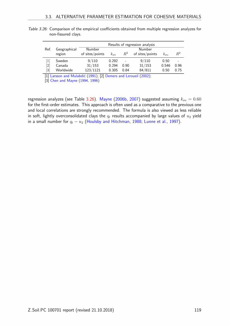
3.3. ALTERNATIVE PARAMETER ESTIMATION FOR COHESIVE MATERIALS
Table 3.26: Comparison of the empirical coefficients obtained from multiple regression analyzes fornon-fissured clays.
Results of regression analysisRef. Geographical Number Number
region of sites/points kσt R2 of sites/points kσe R2
[1] Sweden 9/110 0.292 - 9/110 0.50 -[2] Canada 31/153 0.294 0.90 31/153 0.546 0.96[3] Worldwide 123/1121 0.305 0.84 84/811 0.50 0.75
[1] Larsson and Mulabdic (1991); [2] Demers and Leroueil (2002);[3] Chen and Mayne (1994, 1996)
regression analyzes (see Table 3.26). Mayne (2006b, 2007) suggested assuming kσe = 0.60for the first-order estimates. This approach is often used as a comparative to the previous oneand local correlations are strongly recommended. The formula is also viewed as less reliablein soft, lightly overconsolidated clays the qt results accompanied by large values of u2 yieldin a small number for qt − u2 (Houlsby and Hitchman, 1988; Lunne et al., 1997).
Z Soil.PC 100701 report (revised 21.10.2018) 119
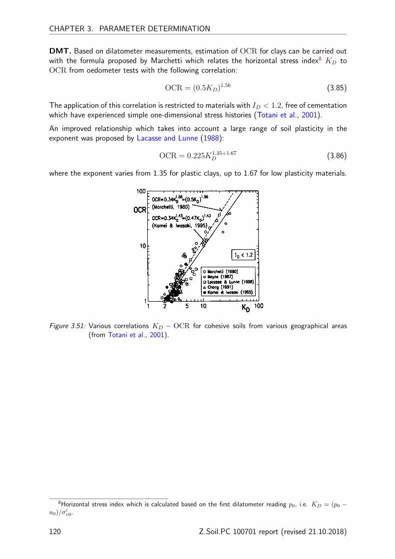
CHAPTER 3. PARAMETER DETERMINATION
DMT. Based on dilatometer measurements, estimation of OCR for clays can be carried outwith the formula proposed by Marchetti which relates the horizontal stress index8 KD toOCR from oedometer tests with the following correlation:
OCR = (0.5KD)1.56 (3.85)
The application of this correlation is restricted to materials with ID < 1.2, free of cementationwhich have experienced simple one-dimensional stress histories (Totani et al., 2001).
An improved relationship which takes into account a large range of soil plasticity in theexponent was proposed by Lacasse and Lunne (1988):
OCR = 0.225K1.35÷1.67D (3.86)
where the exponent varies from 1.35 for plastic clays, up to 1.67 for low plasticity materials.
Figure 3.51: Various correlations KD − OCR for cohesive soils from various geographical areas(from Totani et al., 2001).
8Horizontal stress index which is calculated based on the first dilatometer reading p0, i.e. KD = (p0 −u0)/σ′v0.
120 Z Soil.PC 100701 report (revised 21.10.2018)

3.3. ALTERNATIVE PARAMETER ESTIMATION FOR COHESIVE MATERIALS
3.3.9 Coefficient of earth pressure ”at rest”
The coefficient of earth pressure ”at rest” for normally-consolidated clays can be estimatedthrough Eq.(3.37a) or the similar expression suggested in Brooker & Ireland (1965):
KNC0 = 0.95− sinφ′ (3.87)
For cohesive soils, KNC0 can also be related through empirical correlations with soil plasticity:
KNC0 = 0.19 + 0.233 log IP (Alpan, 1967) (3.88a)
and similarKNC
0 = 0.44 + 0.0042IP (Holtz & Kovacs, 1981) (3.88b)
where IP is the plasticity index in %.
It is commonly known that in cohesive soils the preconsolidation plays an important role andK0 typically increases with the overconsolidation ratio OCR. Estimations of the initial stressstate for overconsolidated soil take a general form:
K0 = KNC0 OCRm (3.89)
where m is a coefficient which for estimation of KNC0 for most practical purposes can be
taken as:m = 0.5 suggested by Meyerhof (1976) (3.90a)
m = sinφ′ suggested in Mayne & Kulhawy (1982) (3.90b)
However, the upper bound value for K0 should be limited by the passive lateral earth pressurecoefficient:
Kp =1 + sinφ
1− sinφ(3.91)
The equations are presented graphically in Fig.3.52 (KNC0 was calculated using Eq. (3.37a)).
SBPT. Approximation of K0 from the self-boring pressuremeter test requires determinationof the horizontal effective stress σ′h0 since the vertical effective stress σ′vo can be estimatedbased on depth, unit weight and groundwater information. In the case of SBPT, the in situtotal horizontal stress can be directly estimated from the ”lift-off” pressure (Jamiolkowskiet al., 1985; Clough et al., 1990; Amar et al., 1991). The ”lift-off” pressure corresponds tothe internal cavity pressure ψ0 when the membrane starts to deform the wall of a borehole,therefore ψ0
∼= σ′h0 + u0 (Figure 3.53). The ”lift-off” is typically estimated based on theaveraging procedure including the measurements of three feeler arms spaced at 120◦ aroundthe instrument (Dalton and Hawkins, 1982; Mair and Wood, 1987). In general, the lateralstress measurements can be considered as fairly accurate in clays, particularly in soft deposits(Jamiolkowski et al., 1985).
Z Soil.PC 100701 report (revised 21.10.2018) 121
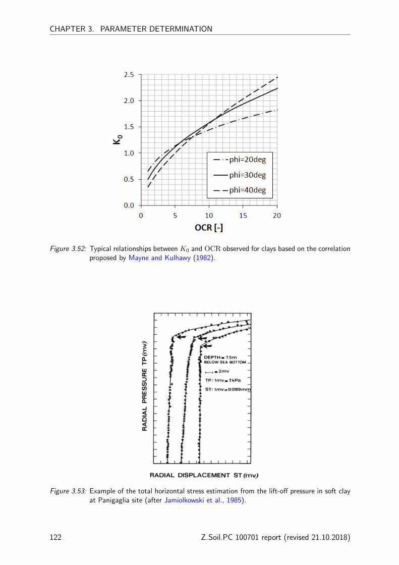
CHAPTER 3. PARAMETER DETERMINATION
Figure 3.52: Typical relationships between K0 and OCR observed for clays based on the correlationproposed by Mayne and Kulhawy (1982).
Figure 3.53: Example of the total horizontal stress estimation from the lift-off pressure in soft clayat Panigaglia site (after Jamiolkowski et al., 1985).
122 Z Soil.PC 100701 report (revised 21.10.2018)
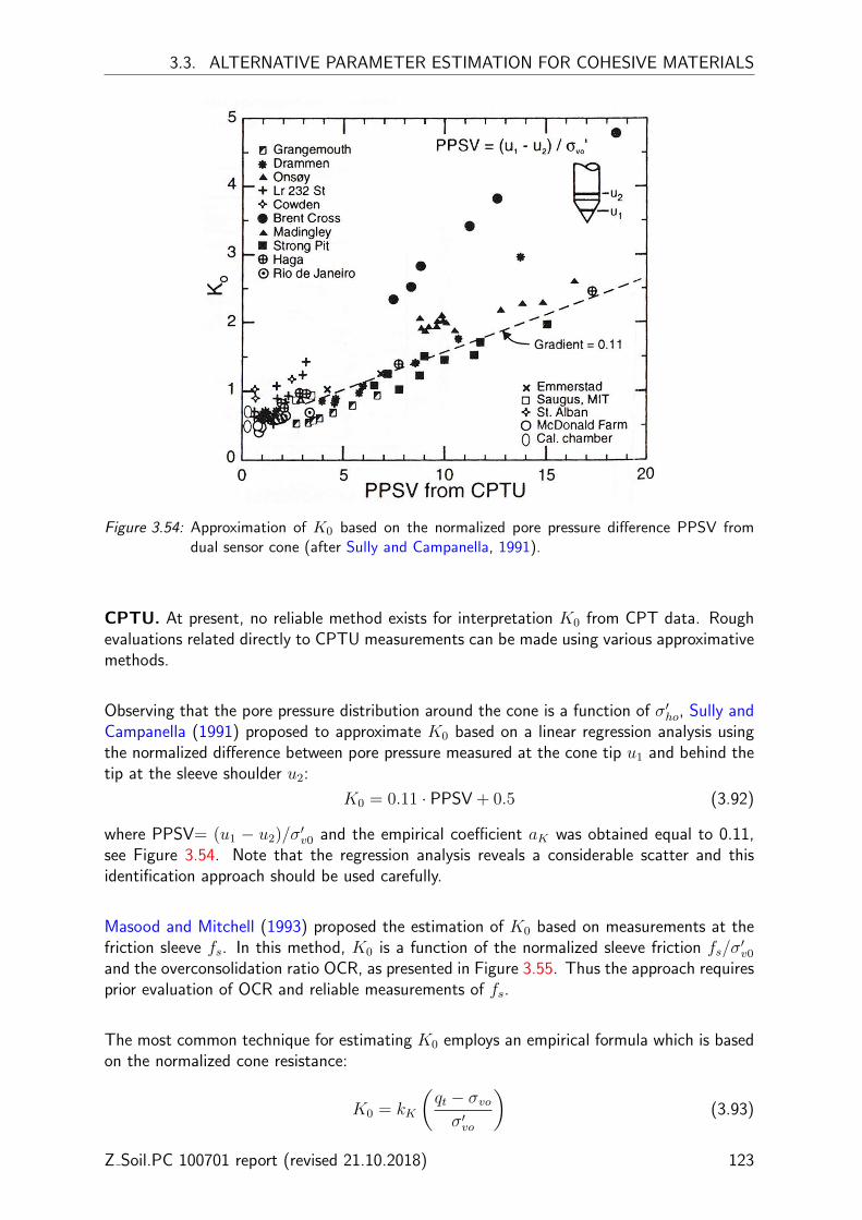
3.3. ALTERNATIVE PARAMETER ESTIMATION FOR COHESIVE MATERIALS
Figure 3.54: Approximation of K0 based on the normalized pore pressure difference PPSV fromdual sensor cone (after Sully and Campanella, 1991).
CPTU. At present, no reliable method exists for interpretation K0 from CPT data. Roughevaluations related directly to CPTU measurements can be made using various approximativemethods.
Observing that the pore pressure distribution around the cone is a function of σ′ho, Sully andCampanella (1991) proposed to approximate K0 based on a linear regression analysis usingthe normalized difference between pore pressure measured at the cone tip u1 and behind thetip at the sleeve shoulder u2:
K0 = 0.11 · PPSV + 0.5 (3.92)
where PPSV= (u1 − u2)/σ′v0 and the empirical coefficient aK was obtained equal to 0.11,see Figure 3.54. Note that the regression analysis reveals a considerable scatter and thisidentification approach should be used carefully.
Masood and Mitchell (1993) proposed the estimation of K0 based on measurements at thefriction sleeve fs. In this method, K0 is a function of the normalized sleeve friction fs/σ
′v0
and the overconsolidation ratio OCR, as presented in Figure 3.55. Thus the approach requiresprior evaluation of OCR and reliable measurements of fs.
The most common technique for estimating K0 employs an empirical formula which is basedon the normalized cone resistance:
K0 = kK
(qt − σvoσ′vo
)(3.93)
Z Soil.PC 100701 report (revised 21.10.2018) 123

CHAPTER 3. PARAMETER DETERMINATION
Figure 3.55: Proposed relationship between K0, fs and OCR Masood and Mitchell (after 1993).
where kK is an empirical coefficient. Using the regression analysis, Kulhawy and Mayne(1990) obtained the value of kK = 0.1 for several K0 values estimated from the self-boringpressuremeter test (SBPT), see Figure 3.56.
Figure 3.56: General K0 correlation for CPTU data proposed by Kulhawy and Mayne (1990)(adapted from Lunne et al., 1997).
DMT. The original correlation for K0 based on the dilatometer data, relative to uncementedclays is (Marchetti, 1980):
K0 =
(KD
1.5
)0.47
− 0.6 (3.94)
In highly cemented clays, the above equation may significantly overestimate K0, since partof KD is due to the cementation.
124 Z Soil.PC 100701 report (revised 21.10.2018)

3.3. ALTERNATIVE PARAMETER ESTIMATION FOR COHESIVE MATERIALS
DMT. K0 can also be interpreted from dilatometer test data. Since the original Marchettirelationship tends to overestimate K0, its estimation can be carried out through the correlationsuggested in Lacasse and Lunne (1988):
K0 = 0.34K0.44÷0.64D (3.95)
where the lower exponent value is associated with highly plastic clays, whereas higher valuesare suggested for for low plasticity materials.
Z Soil.PC 100701 report (revised 21.10.2018) 125

CHAPTER 3. PARAMETER DETERMINATION
3.3.10 Void ratio
Typical values of voids ratio and dry unit weights observed for cohesive soils are provided inTable 3.27 and 3.28.
Table 3.27: Typical values of void ratios and dry unit weights observed in cohesive soils (fromHough, 1969).
Voids ratioe [–]
Soil type Min Max
Silty or sandy clay 0.25 1.8Gap-graded silty clay w. gravel or larger 0.2 1Well-graded gravel/sand/silt/clay 0.13 0.7Clay (30 to 50% of 2microns size) 0.5 2.4Colloidal clay (over 50% of 2microns size) 0.6 12Organic silt 0.55 3Uniform, inorganic silt 0.4 1.1Organic clay (30 to 50% of 2microns size) 0.7 4.4
Table 3.28: Typical values of void ratios and unit weights observed in granular soils (from Terzaghiet al., 1996).
Voids ratio Dry unit weights Wet weightsSoil type e [–] [kN/m3] [kN/m3]
Glacial till, very mixed grained 0.25 20.8 22.7Soft glacial clay 1.2 12 17.4Stiff glacial clay 0.6 16.7 20.3Soft slightly organic clay 1.9 9.1 15.5Soft very organic clay 3 6.7 14.4Soft bentonite 5.2 4.2 12.5
126 Z Soil.PC 100701 report (revised 21.10.2018)
3.4. AUTOMATED ASSISTANCE IN PARAMETER DETERMINATION
3.4 Automated assistance in parameter determination
Virtual Lab v2018 is a highly-interactive module which provides users with:
• assistance in selecting a relevant constitutive law with regards to the general behavior ofthe real material
• first-guess parameter estimation based on field test records
• automated parameter selection (first-guess values of model parameters for soil for anyincomplete or complete specimen data)
• user-engaged parameter selection (interactive parameter selection which involves browsingdifferent parameter correlations including field tests data)
• ranges of parameter values which can be considered in parametric studies
• automated parameter identification from laboratory experimental data
• possibility of running numerical simulations of elementary laboratory tests in order to visu-alize the constitutive model response for the defined model parameters
• possibility of comparing numerical simulations of elementary laboratory tests with curvesobtained in the laboratory
A separated report provides Help to Virtual Lab.
The toolbox is initialized by clicking on Virtual Lab which is visible once one of the followingcontinuum models has been chosen as the material definition (Figure 3.57):
• Mohr-Coulomb
• Hardening-Soil Small Strain
• Cam-Clay
• Cap
Z Soil.PC 100701 report (revised 21.10.2018) 127
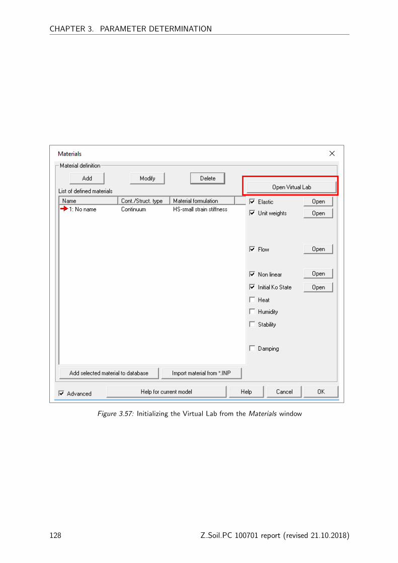
CHAPTER 3. PARAMETER DETERMINATION
Figure 3.57: Initializing the Virtual Lab from the Materials window
128 Z Soil.PC 100701 report (revised 21.10.2018)

Chapter 4
Benchmarks
4.1 Triaxial drained compression test on dense Hostun sand
Files:HS-std-dh-sand-100kPa.inp, HS-small-dh-sand-100kPa.inp,HS-std-dh-sand-300kPa.inp, HS-small-dh-sand-300kPa.inp,HS-std-dh-sand-600kPa.inp, HS-small-dh-sand-600kPa.inp
The following section presents a validation of both HS and HS-small models on a triaxialdrained compression test for Hostun sand. Material properties are taken from PhD thesis byBenz (2007) and are given in the following table:
Parameter Unit Value Parameter Unit Value
Erefur [kPa] 90000 ψ [o] 16.0
Eref50 [kPa] 30000 ft [kPa] 0.0σref [kPa] 100 D [–] 0.0/0.251
m [–] 0.55 M [–] 1.727/1.723νur [–] 0.25 H [kPa] 55967/57055Rf [–] 0.9 OCR [–] 1.0c [kPa] 0.0 Eref
0 [kPa] 270000φ [o] 42.0 γ0.7 [–] 0.0002
The parameters M and H were estimated automatically by the code assuming KNC0 = 0.4
and Eoed = 30000 kPa at reference stress equal to 100 kPa. It must be emphasized that Mand H values will not be equal to the ones given by Benz because of the different hardeninglaw applied to the preconsolidation pressure pc. All results obtained with Z Soil match verywell results published by Benz. The only differences appear in G−γ plots where Z Soil resultsfor standard HS-model are lower than the reference ones. In our opinion, G − γ curves forstandard HS model which were published by Benz, begin at Gur value and are not obtainedfrom the elasto-plastic solution.

CHAPTER 4. BENCHMARKS
(a)σ1
σ3
(ε1) (Z Soil) (b) G(γ) (Z Soil)
(c)σ1
σ3
(ε1) (zoom) (Z Soil) (d) εv(ε1) (Z Soil)
(e) Solution by Benz Benz (2007)
Figure 4.1: Results for the confining pressure σ3 = 100 kPa
130 Z Soil.PC 100701 report (revised 21.10.2018)

4.1. TRIAXIAL DRAINED COMPRESSION TEST ON DENSE HOSTUN SAND
(a)σ1
σ3
(ε1) (Z Soil) (b) G(γ) (Z Soil)
(c)σ1
σ3
(ε1) (zoom) (Z Soil) (d) εv(ε1) (Z Soil)
(e) Solution by Benz Benz (2007)
Figure 4.2: Results for the confining pressure σ3 = 300 kPa
Z Soil.PC 100701 report (revised 21.10.2018) 131

CHAPTER 4. BENCHMARKS
(a)σ1
σ3
(ε1) (Z Soil) (b) G(γ) (Z Soil)
(c)σ1
σ3
(ε1) (zoom) (Z Soil) (d) εv(ε1) (Z Soil)
(e) Solution by Benz Benz (2007)
Figure 4.3: Results for the confining pressure σ3 = 600 kPa
132 Z Soil.PC 100701 report (revised 21.10.2018)

4.2. ISOTROPIC COMPRESSION OF DENSE HOSTUN SAND
4.2 Isotropic compression of dense Hostun sand
File: HS-isotropicCompr.inp
This benchmark is solved analytically for the HS-Std model. The decomposed total strainincrements for the elastic and plastic part in isotropic compression conditions (p = pc) arepresented in the following expression (NB. the increment of total volumetric strain is measuredfrom the initial configuration of equilibrium p0 = pc0 to the current one):
∆εpv =
σref + c cotφ
1−m
[(pco + c cotφ
σref + c cotφ
)1−m
−(
pc + c cotφ
σref + c cotφ
)1−m]
H(4.1)
∆εev =3(1− 2νur)
Erefur
(σref + c cotφ
1−m
)[(pc + c cotφ
σref + c cotφ
)1−m
−(pco + c cotφ
σref + c cotφ
)1−m]
(4.2)
∆εv = ∆εev + ∆εpv (4.3)
Verification was carried out on an single axisymmetric finite element which is subject to anexternal uniformly distributed load varying from q = 50 kN/m2 to q = 250 kN/m2. Theinitial effective stresses are σo = {−50,−50, 0,−50}T kPa. Material data for the denseHostun sand (see section (4.1)) is used in the simulation. Numerical and analytical solutionsare compared in in the following figure.
ISOTROPIC COMPRESSION TEST
0
50
100
150
200
250
300
-0.008 -0.006 -0.004 -0.002 0EPS-V [-]
p [k
Pa]
EXACTZ_SOIL
Z Soil.PC 100701 report (revised 21.10.2018) 133
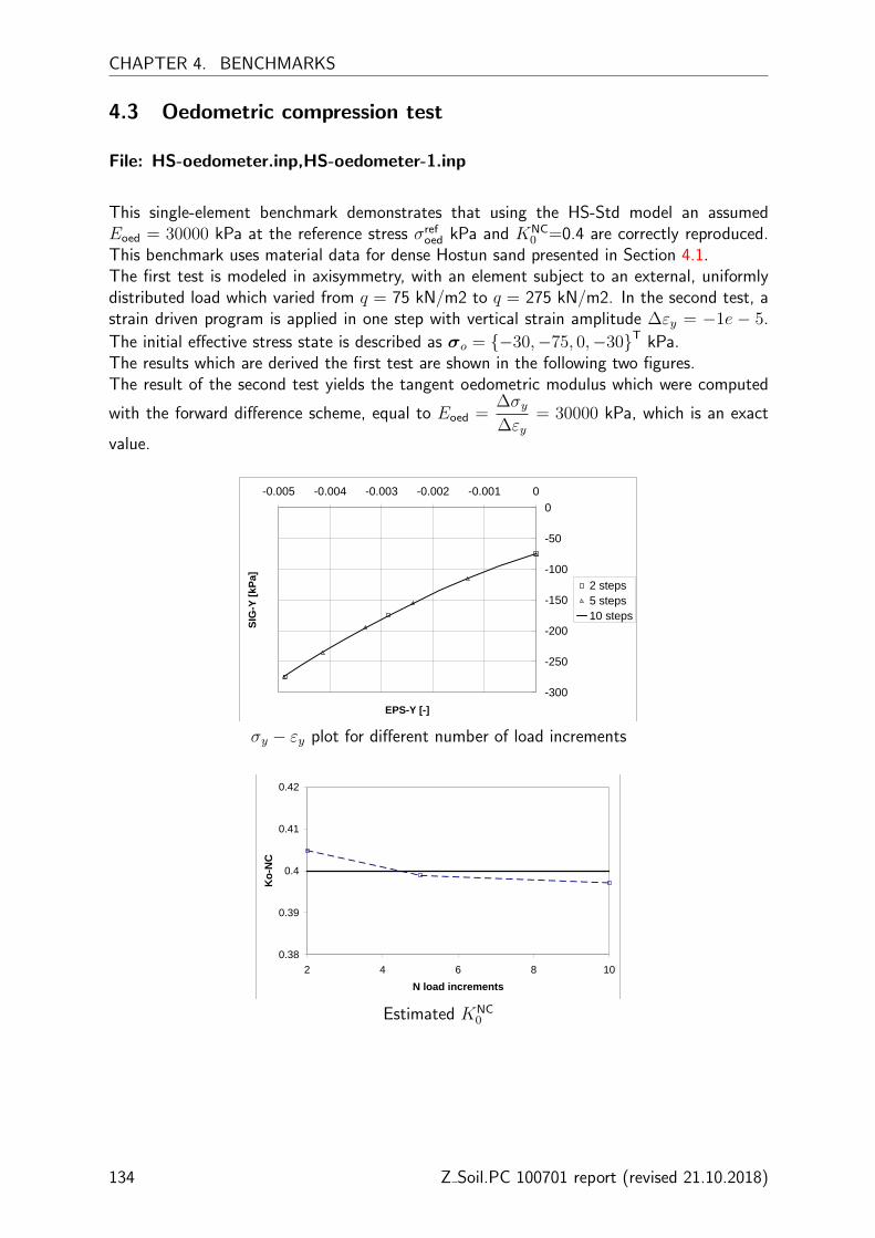
CHAPTER 4. BENCHMARKS
4.3 Oedometric compression test
File: HS-oedometer.inp,HS-oedometer-1.inp
This single-element benchmark demonstrates that using the HS-Std model an assumedEoed = 30000 kPa at the reference stress σref
oed kPa and KNC0 =0.4 are correctly reproduced.
This benchmark uses material data for dense Hostun sand presented in Section 4.1.The first test is modeled in axisymmetry, with an element subject to an external, uniformlydistributed load which varied from q = 75 kN/m2 to q = 275 kN/m2. In the second test, astrain driven program is applied in one step with vertical strain amplitude ∆εy = −1e − 5.
The initial effective stress state is described as σo = {−30,−75, 0,−30}T kPa.The results which are derived the first test are shown in the following two figures.The result of the second test yields the tangent oedometric modulus which were computed
with the forward difference scheme, equal to Eoed =∆σy∆εy
= 30000 kPa, which is an exact
value.
-300
-250
-200
-150
-100
-50
0-0.005 -0.004 -0.003 -0.002 -0.001 0
EPS-Y [-]
SIG
-Y [k
Pa]
2 steps5 steps10 steps
σy − εy plot for different number of load increments
0.38
0.39
0.4
0.41
0.42
2 4 6 8 10N load increments
Ko-
NC
Estimated KNC0
134 Z Soil.PC 100701 report (revised 21.10.2018)

4.4. OEDOMETRIC COMPRESSION TEST - KNC0 -PATH TEST
4.4 Oedometric compression test - KNC0 -path test
This single-element benchmark that HS-Std model is able to correctly reproduce KNC0 -path
for the oedometric test for different values of the friction angle. The results are comparedwith the data obtained with other constitutive models.
The oedometric test on the normally-consolidated soil (qPOP = 0.1 kPa) is modeled in
(a) (b)
Figure 4.4: KNC0 -path test for the HS-Std model and different values of the friction angle φ =
20o, 30o, 40o: a) stress paths in p′ − q plane, b) KNC0 with increasing loading.
axisymmetry, with a single element subject to an external, uniformly distributed load whichvaried from q = 0 kN/m2 to q = 800 kN/m2. The results which are presented in Figure4.4 show that HS-Std model correctly reproduces KNC
0 stress paths which obey the empiricalexpression KNC
0 = 1− sinφ for three different values of the friction angle.
The same model is used to compare the results from the oedometric test using differentconstitutive models: the Modified Cam clay (MCC), the standard Mohr-Coulomb (M-C) andthe Cap model (CAP). Simulations for different models were carried out for the same valueof the friction angle φ = 30o (and equivalent M = 1.2 for the MCC model). Hence, thevalue of cohesion was assumed as c = 0 kPa. The value of Poisson’s ratio was assumedνur = 0.2 for the HS model and ν = 0.3 for other models. Figure 4.5 shows that startingfrom the initial ”zero” stress setup and gradually increasing the vertical stress, only the HSmodel is able to reproduce expected σ′h/σ
′v path. It is so because the parameter M which
defines the shape of the cap surface in the HS-model, is optimized so that the tangent tothe cap surface at the stress reversal point is perpendicular to KNC
0 stress path.
Z Soil.PC 100701 report (revised 21.10.2018) 135
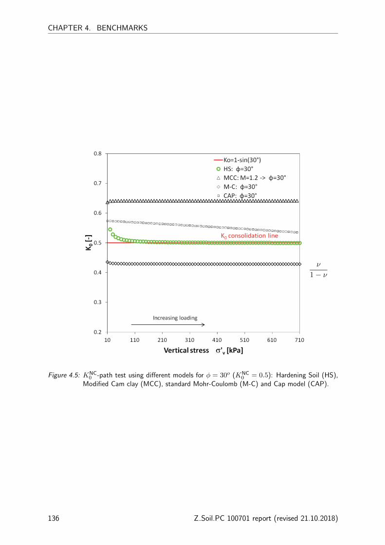
CHAPTER 4. BENCHMARKS
ν
1− ν
Figure 4.5: KNC0 -path test using different models for φ = 30o (KNC
0 = 0.5): Hardening Soil (HS),Modified Cam clay (MCC), standard Mohr-Coulomb (M-C) and Cap model (CAP).
136 Z Soil.PC 100701 report (revised 21.10.2018)

Chapter 5
Case studies
5.1 Excavation in Berlin Sand
File: HS-std-Exc-Berlin-Sand-2phase.inpFile: HS-small-Exc-Berlin-Sand-2phase.inpFile: MC-Exc-Berlin-Sand-2phase.inp
This example demonstrates the importance of modeling excavation problems with the use ofthe Hardening Soil model. The study case presents an analysis of main differences betweenHS-Std, HS-Small and standard Mohr-Coulomb (MC) models based on a numerical simula-tion of a deep excavation in Berlin Sand.
An engineering draft of the problem and the sequence of both excavation and constructionsteps, are given in Figure 5.1. Material data for calibration of sand was taken from Benz(2007) and Schweiger (2002). The data with standard MC model was generated assumingthat stiffness of sand varies according to the power law:
E = 20000√y kPa for y ≤ 20m
E = 60000√y kPa for y > 20m
where y is the depth expressed in [m]. The same strength parameters apply to both the MCmodel and HS models.

CHAPTER 5. CASE STUDIES
Figure 5.1: An engineering draft and the sequence of both excavation and construction stages forthe deep excavation in Berlin sand.
Sequence of stages:
1. Generating an initial stress state for an assumed K in situ0 in sand layers
2. Installation of the diaphragm wall
3. Lowering the ground water level in the excavated zone up to the elevation -17.90m
4. Excavation step 1 (up to -4.80m)
5. Introducing the first row of anchors (distance 2.30 m) and applying the prestress P0 = 768kN
6. Excavation step 2 (up to -9.30m)
7. Introducing of the second row of anchors (distance 1.35 m) and and applying the prestressP0 = 945 kN
8. Excavation step 3 (up to -14.35m)
9. Introducing of the third row of anchors (distance 1.35 m) and and applying the prestressP0 = 980 kN
10. Excavation step 4 (up to -16.80m)
138 Z Soil.PC 100701 report (revised 21.10.2018)
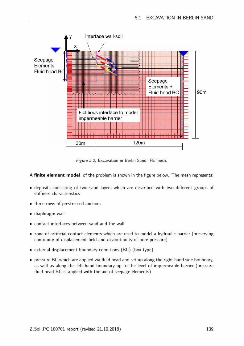
5.1. EXCAVATION IN BERLIN SAND
Figure 5.2: Excavation in Berlin Sand: FE mesh.
A finite element model of the problem is shown in the figure below. The mesh represents:
• deposits consisting of two sand layers which are described with two different groups ofstiffness characteristics
• three rows of prestressed anchors
• diaphragm wall
• contact interfaces between sand and the wall
• zone of artificial contact elements which are used to model a hydraulic barrier (preservingcontinuity of displacement field and discontinuity of pore pressure)
• external displacement boundary conditions (BC) (box type)
• pressure BC which are applied via fluid head and set up along the right hand side boundary,as well as along the left hand boundary up to the level of impermeable barrier (pressurefluid head BC is applied with the aid of seepage elements)
Z Soil.PC 100701 report (revised 21.10.2018) 139
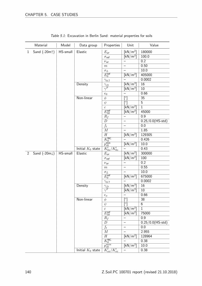
CHAPTER 5. CASE STUDIES
Table 5.1: Excavation in Berlin Sand: material properties for soils
Material Model Data group Properties Unit Value
1 Sand (-20m↑) HS-small Elastic Eur [kN/m2] 180000σref [kN/m2] 100.0νur – 0.2m – 0.50σL – 10.0Eref
0 [kN/m2] 405000γ0.7 – 0.0002
Density γD [kN/m3] 16γF [kN/m3] 10e0 – 0.66
Non-linear φ [◦] 35ψ [◦] 5c [kN/m2] 1Eref
50 [kN/m2] 45000Rf – 0.9D – 0.25/0.0(HS-std)ft – 0.0M – 1.85H [kN/m2] 129305KNC
0 – 0.426pminc0 [kN/m2] 10.0
Initial K0 state K ′0x/K ′0z – 0.43
2 Sand (-20m↓) HS-small Elastic Eur [kN/m2] 300000σref [kN/m2] 100νur – 0.2m – 0.55σL – 10.0Eref
0 [kN/m2] 675000γ0.7 – 0.0002
Density γD [kN/m3] 16γF [kN/m3] 10eo – 0.66
Non-linear φ [◦] 38ψ [◦] 6c [kN/m2] 1Eref
50 [kN/m2] 75000Rf – 0.9D – 0.25/0.0(HS-std)ft – 0.0M – 2.955H [kN/m2] 128964KNC
0 – 0.38pminc0 [kN/m2] 10.0
Initial K0 state K ′ox/K ′oz – 0.38
140 Z Soil.PC 100701 report (revised 21.10.2018)

5.1. EXCAVATION IN BERLIN SAND
Table 5.2: Excavation in Berlin Sand: material properties for the diaphragm wall, anchors andinterfaces
Material Model Data group Properties Unit Value
3 Wall Beams Elastic E [kN/m2] 30000000ν – 0.15
Density Unit weight [kN/m3] 24Geometry Interval [m] 1.0
A [m2] 0.8Iz [m4] 0.0426667
4 Anchors Truss Elastic E [kN/m2] 210000000Density Unit weight [kN/m3] 0.0Geometry Interval [m] 2.3
A [m2] 0.0015
5 Anchors Truss Elastic E [kN/m2] 210000000Density Unit weight [kN/m3] 0.0Geometry Interval [m] 1.35
A [m2] 0.0015
6 Anchors Truss Elastic E [kN/m2] 210000000Density Unit weight [kN/m3] 0.0Geometry Interval [m] 1.35
A [m2] 0.0015
7 Interface Contact Non-linear φ [◦] 28ψ [◦] 0c [kN/m2] 0.0
Z Soil.PC 100701 report (revised 21.10.2018) 141

CHAPTER 5. CASE STUDIES
The chart below presents four unloading functions which are defined and associated withthe excavated elements in order to gradually unload each excavated region. Note that thesame unloading functions must be applied to interface elements adjacent to the excavatedcontinuum. All existence functions and unloading functions which are applied for excavatedzones of sand are shown in the chart below.
30.0m
t2 4 6 8EXF1
t2 4 6 8EXF2
t2 4 6 8EXF3
t2 4 6 8EXF4
t2 4 6 8UF3
t2 4 6 8UF2
t2 4 6 8UF1
t2 4 6 8UF4
Figure 5.3: Excavation in Berlin Sand: unloading functions
142 Z Soil.PC 100701 report (revised 21.10.2018)
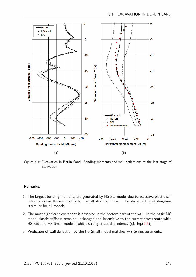
5.1. EXCAVATION IN BERLIN SAND
(a) (b)
Figure 5.4: Excavation in Berlin Sand: Bending moments and wall deflections at the last stage ofexcavation
Remarks:
1. The largest bending moments are generated by HS-Std model due to excessive plastic soildeformation as the result of lack of small strain stiffness . The shape of the M diagramsis similar for all models.
2. The most significant overshoot is observed in the bottom part of the wall. In the basic MCmodel elastic stiffness remains unchanged and insensitive to the current stress state whileHS-Std and HS-Small models exhibit strong stress dependency (cf. Eq.(2.5)).
3. Prediction of wall deflection by the HS-Small model matches in situ measurements.
Z Soil.PC 100701 report (revised 21.10.2018) 143

CHAPTER 5. CASE STUDIES
(a)
(b)
Figure 5.5: Excavation in Berlin Sand: Soil deformations at last stage of excavation(a) vertical heaving of subsoil, (b) settlements of the ground behind the wall (y = 0 m)
Remarks:
1. The HS-Std and MC models with variable stiffness generate similar heavings.
2. Vertical heaving generated by The HS-Small model is significantly reduced with respect toresults which are generated by HS-Std and MC models
3. The MC model results in an unrealistic lifting of the retaining wall associated with unloadingof the bottom of an excavation. Settlements behind the wall are realistically generatedwith HS-Std and HS-Small models.
144 Z Soil.PC 100701 report (revised 21.10.2018)
5.2. TWIN TUNNELS EXCAVATION IN LONDON CLAY
5.2 Twin tunnels excavation in London Clay
File: HS-std-Exc-London-Clay-2phase.inpFile: HS-small-Exc-London-Clay-2phase.inpFile: MC-Exc-London-Clay-2phase-E3600z.inpFile: MC-Exc-London-Clay-2phase-E6000z.inp
This example demonstrates the importance of modeling tunnel construction problems withthe use of advanced constitutive models such as Hardening Soil models which allows modelingpre-failure non-linear stiffness. The study highlights the differences in predictions of subsurfacedisplacements during tunnel excavations in the stiff, heavily overconsolidated London Claymodeled with:
• Linear-elastic, perfectly plastic Mohr-Coulomb model.
• Non-linear elastic, perfectly plastic models: HS-Std and HS-SmallStrain.
This study reanalyzes the excavation model of the twin Jubilee Line Extension Project tun-nels beneath St James’s Park (London, UK) which has been reported in the original paper byAddenbrooke et al. (1997). The predictions of displacements obtained with the HardeningSoil models are additionally compared with the results obtained by Addenbrooke et al. (1997)for the isotropic non-linear elastic model J4 and field data.
The problem statement, i.e. subsurface stratigraphy and the orientation of tunnels is pre-sented in Figure 5.6. The following paragraphs present the analysis details, the excava-tion/construction stages and the material data assumed in the analyzes.
Z Soil.PC 100701 report (revised 21.10.2018) 145
CHAPTER 5. CASE STUDIES
Analysis details
• analysis type: plain strain deformation + flow
• driver type: consolidation
• mesh: Figure 5.7
• constitutive models:
F Sand: linear elastic
F Thames Gravel: linear elastic Mohr-Coulomb (M-C)
F London Clay: three variants (i) M-C, (ii) Hardening Soil Standard (HS-Std), (iii) Hard-ening Soil Small Strain (HS-SmallStrain)
F Woolwich and Reading Bed Clay: M-C
Excavation/construction stages
1. Generating the initial state in substrata for the assumed Kinsitu0 across the FE mesh pre-
sented in Figure 5.7
2. Installation of seepage elements around the tunnel which permits free flow simulating drainsand excavation of the westbound tunnel with gradual unloading - 100% unloading after 8hours
3. Installation of the 1st tunnel lining at 75% of unloading; parameter for tunnel lining aregiven in Table 5.7 and removing seepage elements
4. Consolidation during 8.5 months
5. Installation of seepage elements around the tunnel which permits free flow simulating drainsand excavation of the eastbound tunnel during 8 hours with gradual unloading
6. Installation of the 2nd tunnel lining at 70% of unloading and removing seepage elements
7. Consolidation
146 Z Soil.PC 100701 report (revised 21.10.2018)
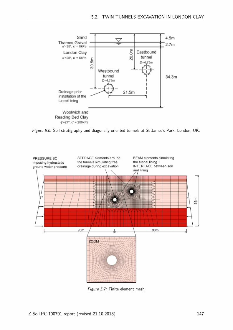
5.2. TWIN TUNNELS EXCAVATION IN LONDON CLAY
Figure 5.6: Soil stratigraphy and diagonally oriented tunnels at St James’s Park, London, UK.
Figure 5.7: Finite element mesh
Z Soil.PC 100701 report (revised 21.10.2018) 147

CHAPTER 5. CASE STUDIES
Material data
• Unit weights - see Table 5.3
• Stiffness parameters
F for HS models - E0, Eur, E50 and γ0.7 calibrated using laboratory ε1− q data points forthe isotropically consolidated undrained extension triaxial test (CIEU) at p′0 = 750 kPa,as shown in Figure 5.10. The constant m was assumed for London Clay equal to 0.75 asreported in Viggiani and Atkinson (1995). The stiffness parameters are given in Table5.5. A similar value of E0 to the calibrated E0 = 390 MPa has been also reported byGasparre (2005).
F for the M-C model: two variants for E have been considered (see Table 5.4)Set 1: E varying with depth z in meters (E = 6000z) as in the original paper byAddenbrooke et al. (1997),Set 2: profile for E adapted to the Eur profile assumed for HS models (i.e. E = 3600z),as graphically presented in Figure 5.8.
• Strength and plastic potential parameters - typical values for London Clay (see Table 5.3)have been adapted from the original paper (Addenbrooke et al., 1997) for all consideredmodels.
• Initial state parameters (see Table 5.6)
F the value of the overconsolidation ratio OCR for London Clay was assumed equal to 15as it is typically observed for depths around 20-30 meters.
F although the estimates of K in situ0 for the London Clay are typically reported of around
1.5, the value K0 = 1.0 has been adopted in the analysis. It was observed that theisotropic Hardening Soil models may give incorrect predictions for K0 >> 1.0 sincestiffness in the model depends on the minor principal stress (maximal settlements werenot observed in the tunnel axis but on its sides for K0 = 1.5). The comparative resultsproduced by model J4 in Addenbrooke et al. (1997) were obtained for K0 = 1.5.
• Permeability - sand and gravel were modelled as highly permeable materials, whereas clayeysoils were attributed with an anisotropic permeability decreasing with depth, as shown inFigure 5.9. The fluid bulk modulus was assumed equal to βf = 2.2 GPa.
• Characteristics for the tunnel lining which were adopted after the original paper are sum-marized in Table 5.7.
148 Z Soil.PC 100701 report (revised 21.10.2018)

5.2. TWIN TUNNELS EXCAVATION IN LONDON CLAY
Figure 5.8: Variation of the unloading-reloading modulus E (Eur) with depth for different modelsconsidered in the study.
Figure 5.9: Permeability profile assumed in the analysis.
Z Soil.PC 100701 report (revised 21.10.2018) 149

CHAPTER 5. CASE STUDIES
Comments:
• Small strain nonlinear models, HS-SmallStrain and J4, well match laboratory data points (in red)both in the very small strain (up to 0.01%) and in the small strains (between 0.01 and 0.4%.
• HS-Std acceptably fits laboratory data at small strains, i.e. from 0.1%).
• M-C model fitted to laboratory data at 0.1% of axial strain strongly overestimates soil stiffnesswith the increasing axial strain.
(a) Very small strains (b) Small strains
Figure 5.10: Stress-strain curves: comparison between non-linear models (HS-Std, HS-SmallStrain,and J-4 model), linear Mohr-Coulomb model and laboratory test data points obtainedin the isotropically consolidated undrained extension test (p′0 = 750 kPa).
Figure 5.11: Variation of the undrained secant stiffness-strain curve ε1−Euds : comparison between
numerical models and laboratory data points obtained in the isotropically (CIEU) andanisotropically (CAEU) consolidated undrained extension tests (p′0 = 750 kPa).
150 Z Soil.PC 100701 report (revised 21.10.2018)

5.2. TWIN TUNNELS EXCAVATION IN LONDON CLAY
Comments:
• In practical applications, linear models may underestimate excess pore water pressure at verysmall strains.
• In consolidation analyzes, M-C model may overestimate excess pore water pressure in the zonesof small strain (in this example beyond the axial strain of 0.1%.
(a) Very small strains (b) Small strains
Figure 5.12: Pore pressure-strain curves: comparison between non-linear models (HS-Std, HS-SmallStrain, and J-4 model), linear Mohr-Coulomb model and laboratory test datapoints obtained in the isotropically consolidated undrained extension test (p′0 = 750kPa).
Z Soil.PC 100701 report (revised 21.10.2018) 151
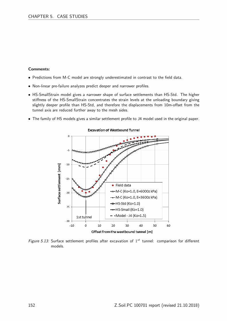
CHAPTER 5. CASE STUDIES
Comments:
• Predictions from M-C model are strongly underestimated in contrast to the field data.
• Non-linear pre-failure analyzes predict deeper and narrower profiles.
• HS-SmallStrain model gives a narrower shape of surface settlements than HS-Std. The higherstiffness of the HS-SmallStrain concentrates the strain levels at the unloading boundary givingslightly deeper profile than HS-Std, and therefore the displacements from 10m-offset from thetunnel axis are reduced further away to the mesh sides.
• The family of HS models gives a similar settlement profile to J4 model used in the original paper.
Figure 5.13: Surface settlement profiles after excavation of 1st tunnel: comparison for differentmodels.
152 Z Soil.PC 100701 report (revised 21.10.2018)

5.2. TWIN TUNNELS EXCAVATION IN LONDON CLAY
Comments:
• Decreasing K0 to 0.8 pronounces the effect of smaller horizontal stresses by bringing closer thenumerical results to the field data.
• The results obtained for K0 = 1.2 resemble the settlement profile which was obtained with J4model for K0 = 1.5 (cf. Figure 5.13).
Figure 5.14: Surface settlement profiles after excavation of 1st tunnel: HS-SmallStrain response fordifferent K0.
Z Soil.PC 100701 report (revised 21.10.2018) 153
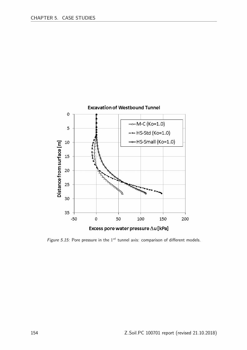
CHAPTER 5. CASE STUDIES
Figure 5.15: Pore pressure in the 1st tunnel axis: comparison of different models.
154 Z Soil.PC 100701 report (revised 21.10.2018)

5.2. TWIN TUNNELS EXCAVATION IN LONDON CLAY
Comments:
• A slight asymmetry in the field data is accordingly reproduced by all models.
• The family of HS models significantly better reproduces the shape of the surface settlement profilein contrast to the M-C model.
Figure 5.16: Surface settlement profiles after excavation of 2nd tunnel: comparison for differentmodels.
Z Soil.PC 100701 report (revised 21.10.2018) 155
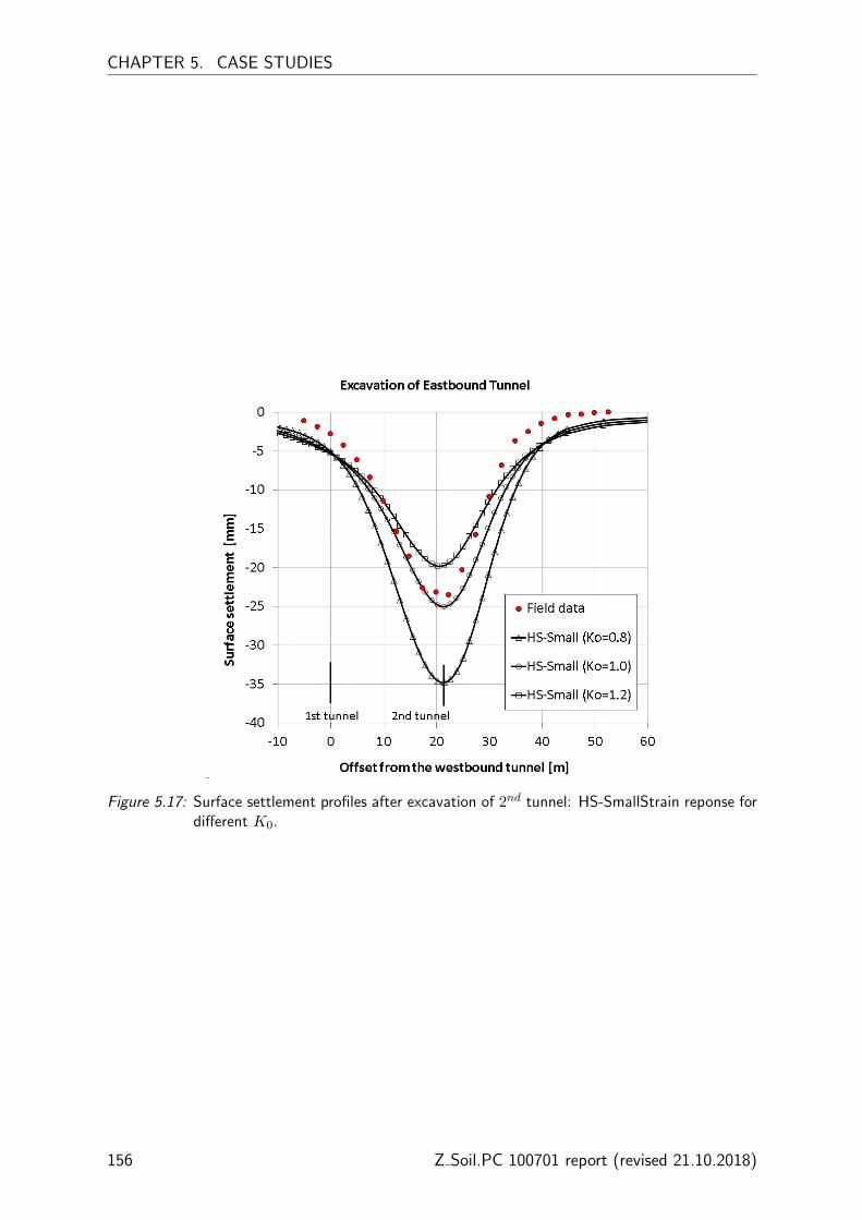
CHAPTER 5. CASE STUDIES
Figure 5.17: Surface settlement profiles after excavation of 2nd tunnel: HS-SmallStrain reponse fordifferent K0.
156 Z Soil.PC 100701 report (revised 21.10.2018)
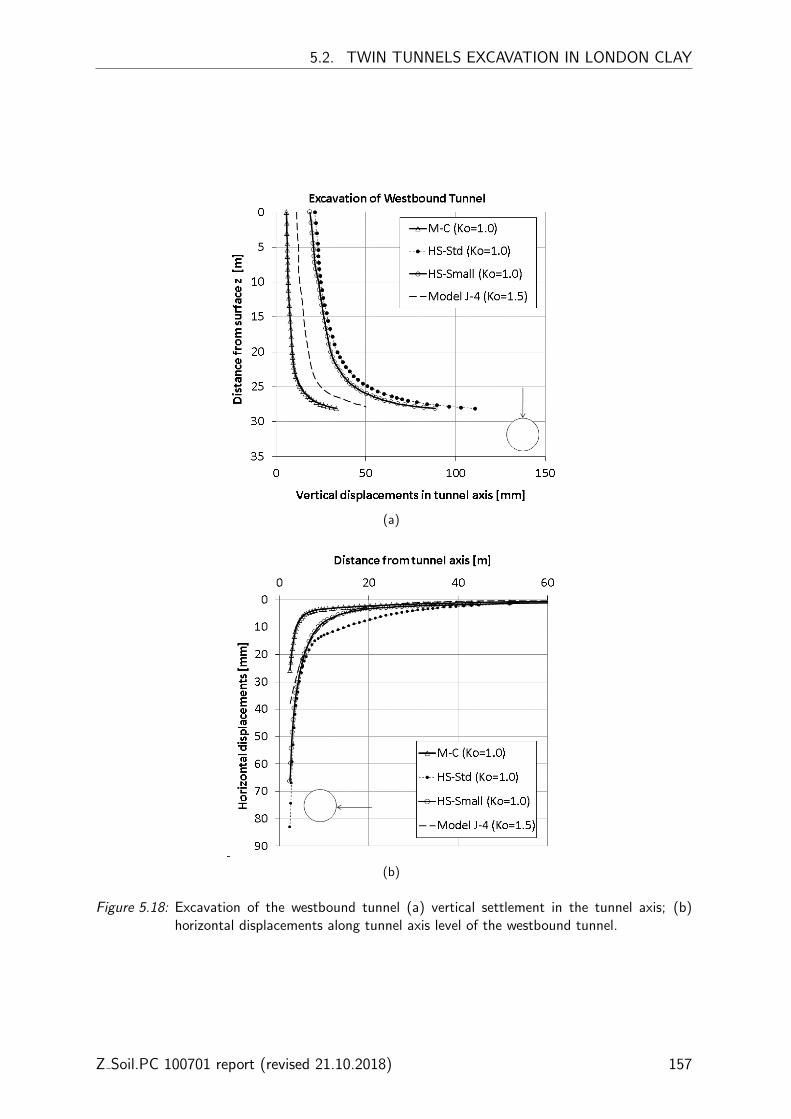
5.2. TWIN TUNNELS EXCAVATION IN LONDON CLAY
(a)
(b)
Figure 5.18: Excavation of the westbound tunnel (a) vertical settlement in the tunnel axis; (b)horizontal displacements along tunnel axis level of the westbound tunnel.
Z Soil.PC 100701 report (revised 21.10.2018) 157

CHAPTER 5. CASE STUDIES
Comments:
• In general, M-C produces smaller vertical and horizontal displacements in the tunnel axes thannon-linear models.
• Unlike to HS models, the model J4 does not automatically return high stiffness behavior onloading reversal occurring during consolidation after 1st excavation, the displacements profilesfor 2nd excavation are smaller than those obtained with HS models. However, the results by HSmodels reveal accordance with the J4 model for which the strains were zeroed across the entiremesh prior to 2nd excavation (J40).
(a)
(b)
Figure 5.19: Excavation of the eastbound tunnel (a) vertical settlement in the tunnel axis; (b)horizontal displacements along tunnel axis level of the eastbound tunnel.
158 Z Soil.PC 100701 report (revised 21.10.2018)

5.2. TWIN TUNNELS EXCAVATION IN LONDON CLAY
Table 5.3: Unit weight, permeability, yield surface and plastic potential parameters for Mohr-Coulomb and HS-models.
Sand Gravel London Clay Woolwich andReading Clay
Strength Linear c′ = 0 kPa c′ = 5.0 kPa c′ = 200 kPaparameters elastic φ′ = 35o φ′ = 25o φ′ = 27o
Angle of dilatation elastic ψ = 17.5o ψ = 12.5o ψ = 13.5o
Bulk unit weight γdry = 18 γsat = 20 γsat = 20 γsat = 20kN/m3 γsat = 20
Permeability coeffi-cient m/s
10−5 10−4 see Fig. 5.9 see Fig. 5.9
Table 5.4: Elastic parameters of soil for linear elastic models, varying with depth below groundsurface, z in meters.
Sand Gravel LondonClay
Woolwich and Read-ing Clay
Poisson’s ratio, υ 0.3 0.2 0.2 0.2Young’s modulus, EkPaset 1 ∗∗ 5000 6000z 6000z ∗ 6000zset 2 ∗∗ 5000 6000z 3600z 6000z∗ E moduli of London Clay for HS models are provided in Table 5.5.∗∗ set 1: values of E modulus from the reference paper; set 2: profile of Emodulus for London Clay similar to the profile of Eur obtained for the HS modelsas shown in Figure 5.8.
Table 5.5: Stiffness parameters of London Clay for HS models at the reference stress σref = 360kPa.
E0 [MPa] γ0.7 [-] Eur [MPa] E50 [MPa] m [-]
390 3e− 004 75 35 0.75
Table 5.6: Initial state parameters assumed in this study.
KNC0 [-] KSR
0 [-] K0 [-] OCR [-]
Sand 0.5 -Gravel 0.5 -London Clay 0.58 0.58 1.0 15Woolwich and Read-ing Clay
1.0 -
Z Soil.PC 100701 report (revised 21.10.2018) 159
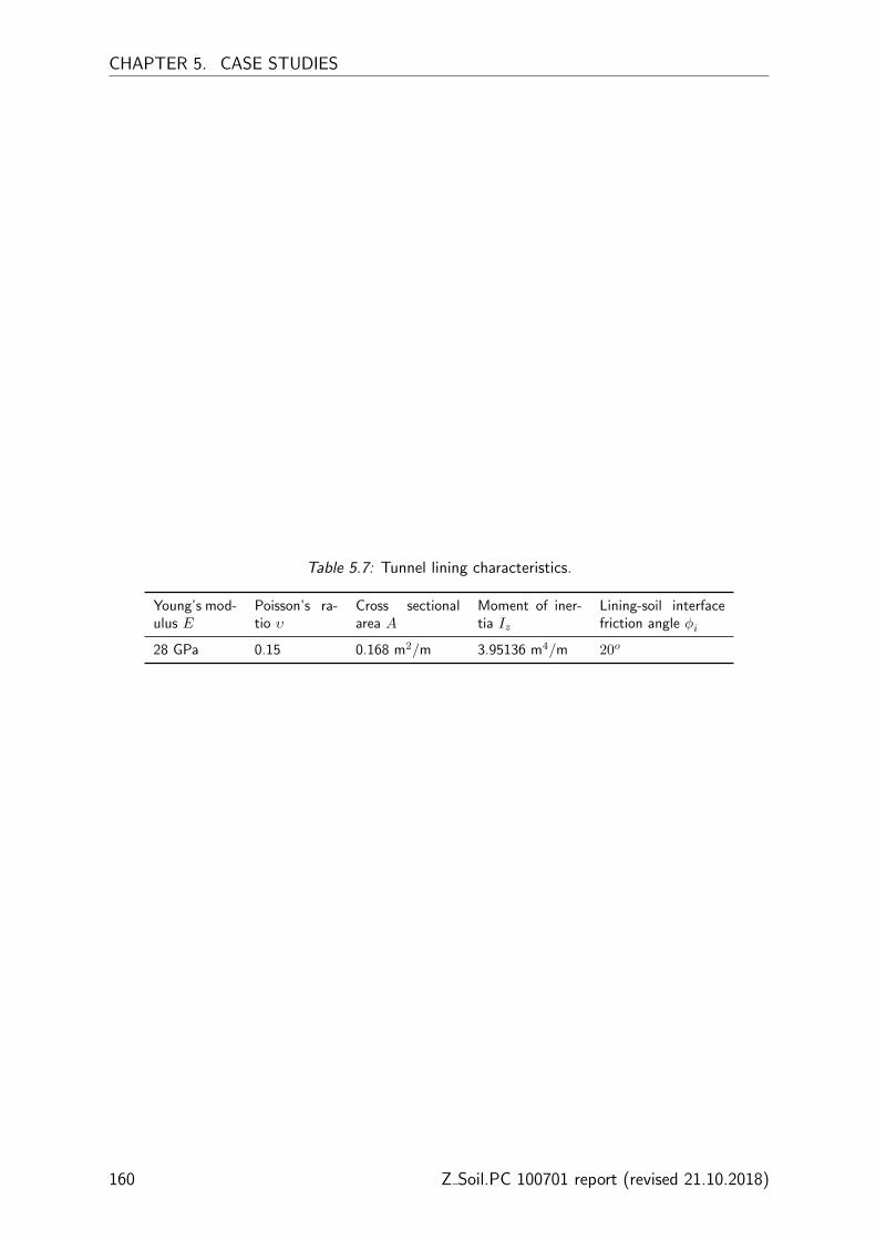
CHAPTER 5. CASE STUDIES
Table 5.7: Tunnel lining characteristics.
Young’s mod-ulus E
Poisson’s ra-tio υ
Cross sectionalarea A
Moment of iner-tia Iz
Lining-soil interfacefriction angle φi
28 GPa 0.15 0.168 m2/m 3.95136 m4/m 20o
160 Z Soil.PC 100701 report (revised 21.10.2018)
5.3. SPREAD FOOTING ON OVERCONSOLIDATED SAND
5.3 Spread footing on overconsolidated Sand
File: HS-small-Foot-Berlin-Sand-2phase.inpFile: MC-Footing-Texas-Sand-2phase EurVar.inp
A verification of the HS-SmallStrain model for a quadratic footing load test is demonstratedin this section. This load test examines the model in terms of its sensitivity to loading andunloading modes applied to overconsolidated sand. This simple boundary value problem alsoillustrates:
• Combined parameter identification from triaxial tests and dilatometer tests
• Interpretation of laboratory and in situ measurements
• Imposing soil stress history through the qPOP (obtaining a variable OCR profile)
• Imposing a variable K0 profile
• Sensitivity of numerical prediction to small-strain stiffness parameters
• Sensitivity of numerical prediction to initial stress setup
The study case demonstrates main differences between HS-Std, HS-Small and standard Mohr-Coulomb (MC) for the analyzes of footing.
Problem statement.
A number of load tests on quadratic footing were performed at Texas A&M University’sNational Geotechnical Site (Briaud and Gibbens, 1997). In this example, the measurementsderived from a load test of 3x3m ”North” footing are compared to numerical predictions.The test setup and soil stratigraphy is presented in Figure 5.20. The subsoil mainly consistsof sandy clay to silty sand layers and it has been confirmed by the interpreted DMT data(see Figure 5.26(a)). Vertical displacements were measured at the corners of the quadraticfooting.
Z Soil.PC 100701 report (revised 21.10.2018) 161

CHAPTER 5. CASE STUDIES
Figure 5.20: A draft of the test setup and soil stratigraphy at A&M University’s National Geotech-nical Site in Texas.
Parameter identification from a triaxial test. The parameters for the HS model havebeen determined from available triaxial compression tests for two sampling depths 0.6m and3.0m, and three confining pressures 34.5, 138 and 345kPa. The results from several resonantcolumn tests with the confining pressure 100kPa have been used to evaluate the order ofmagnitude of small strain characteristics. The reader can analyze parameter identification inthe spreadsheet presented in Table 5.8. Note that the determination of φ′ and c′ was carriedout only for 34.5kPa and 138kPa tests since the ultimate state (failure deviatoric stress qf )was not achieved at 345kPa.A comparison of numerical results and experimental data derived from triaxial compressiontests is presented in Figure 5.22. Note that the preconsolidated state of soil specimens wastaken into account in the triaxial test simulations by applying the initial value of the minimalpreconsolidation pressure pc0 = 250kPa. The value was evaluated assuming that:
σ′v0 = 14.9kN/m3 × 3.0m = 44.7kPa
and applying an estimated qPOP (see Figure 5.25):
σ’SRy = σ′vc = σ′v0 + qPOP = 44.7kPa + 350kPa = 394.7kPa cf. Eq.(2.26a)
σ’SRx = σ′v0 ·KSR
0 = 394.7kPa ×0.41 = 161.8kPa
162 Z Soil.PC 100701 report (revised 21.10.2018)
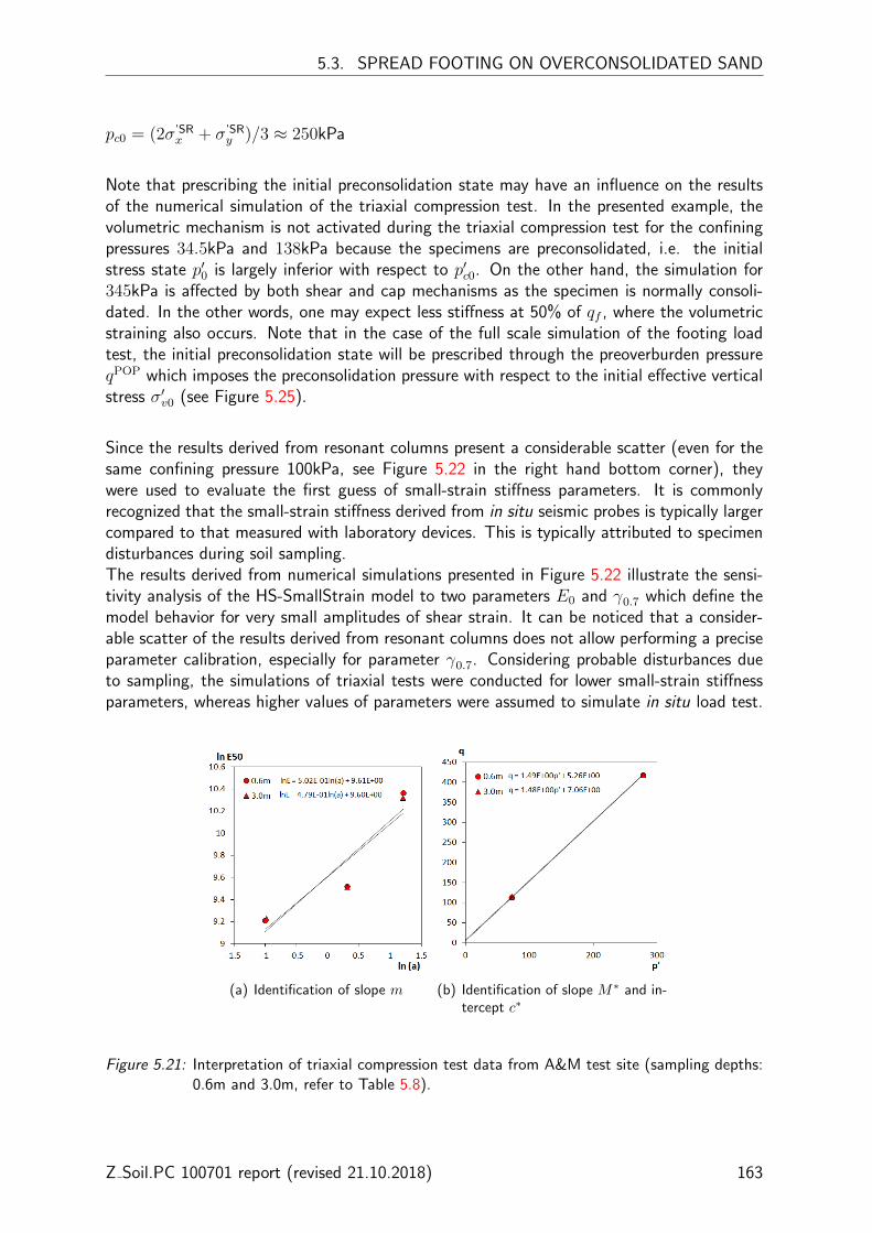
5.3. SPREAD FOOTING ON OVERCONSOLIDATED SAND
pc0 = (2σ’SRx + σ’SR
y )/3 ≈ 250kPa
Note that prescribing the initial preconsolidation state may have an influence on the resultsof the numerical simulation of the triaxial compression test. In the presented example, thevolumetric mechanism is not activated during the triaxial compression test for the confiningpressures 34.5kPa and 138kPa because the specimens are preconsolidated, i.e. the initialstress state p′0 is largely inferior with respect to p′c0. On the other hand, the simulation for345kPa is affected by both shear and cap mechanisms as the specimen is normally consoli-dated. In the other words, one may expect less stiffness at 50% of qf , where the volumetricstraining also occurs. Note that in the case of the full scale simulation of the footing loadtest, the initial preconsolidation state will be prescribed through the preoverburden pressureqPOP which imposes the preconsolidation pressure with respect to the initial effective verticalstress σ′v0 (see Figure 5.25).
Since the results derived from resonant columns present a considerable scatter (even for thesame confining pressure 100kPa, see Figure 5.22 in the right hand bottom corner), theywere used to evaluate the first guess of small-strain stiffness parameters. It is commonlyrecognized that the small-strain stiffness derived from in situ seismic probes is typically largercompared to that measured with laboratory devices. This is typically attributed to specimendisturbances during soil sampling.The results derived from numerical simulations presented in Figure 5.22 illustrate the sensi-tivity analysis of the HS-SmallStrain model to two parameters E0 and γ0.7 which define themodel behavior for very small amplitudes of shear strain. It can be noticed that a consider-able scatter of the results derived from resonant columns does not allow performing a preciseparameter calibration, especially for parameter γ0.7. Considering probable disturbances dueto sampling, the simulations of triaxial tests were conducted for lower small-strain stiffnessparameters, whereas higher values of parameters were assumed to simulate in situ load test.
(a) Identification of slope m (b) Identification of slope M∗ and in-tercept c∗
Figure 5.21: Interpretation of triaxial compression test data from A&M test site (sampling depths:0.6m and 3.0m, refer to Table 5.8).
Z Soil.PC 100701 report (revised 21.10.2018) 163
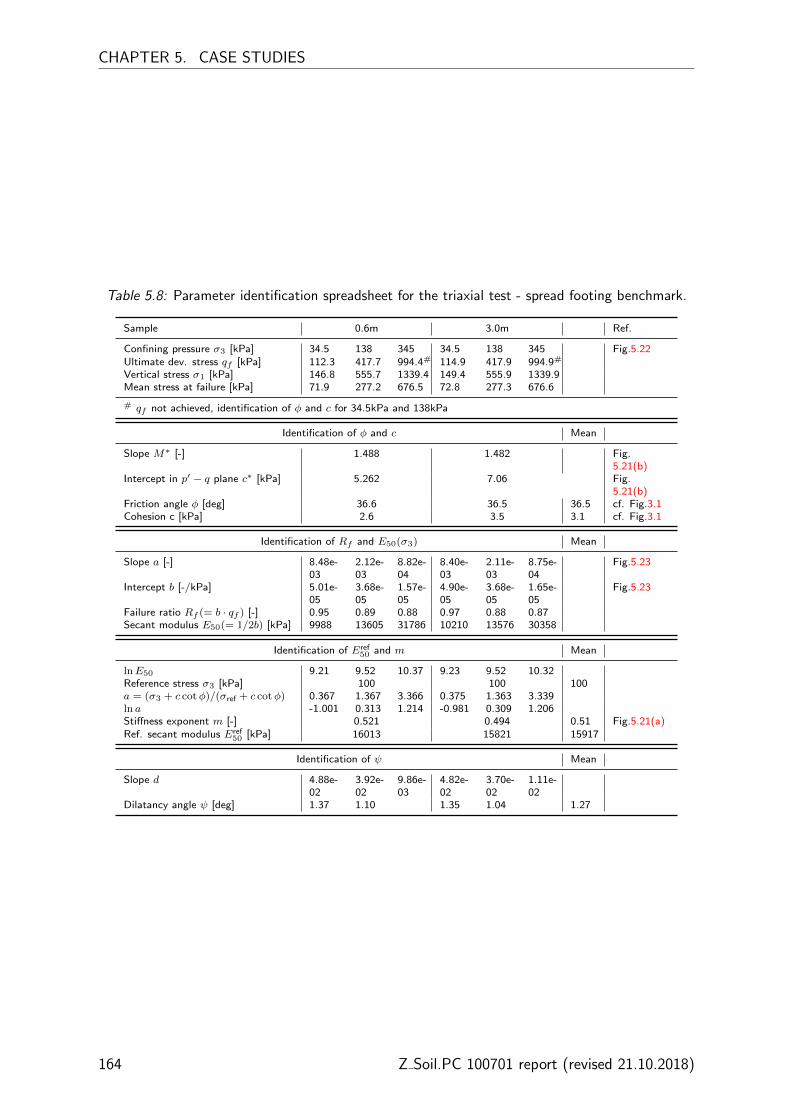
CHAPTER 5. CASE STUDIES
Table 5.8: Parameter identification spreadsheet for the triaxial test - spread footing benchmark.
Sample 0.6m 3.0m Ref.
Confining pressure σ3 [kPa] 34.5 138 345 34.5 138 345 Fig.5.22Ultimate dev. stress qf [kPa] 112.3 417.7 994.4# 114.9 417.9 994.9#
Vertical stress σ1 [kPa] 146.8 555.7 1339.4 149.4 555.9 1339.9Mean stress at failure [kPa] 71.9 277.2 676.5 72.8 277.3 676.6
# qf not achieved, identification of φ and c for 34.5kPa and 138kPa
Identification of φ and c Mean
Slope M∗ [-] 1.488 1.482 Fig.5.21(b)
Intercept in p′ − q plane c∗ [kPa] 5.262 7.06 Fig.5.21(b)
Friction angle φ [deg] 36.6 36.5 36.5 cf. Fig.3.1Cohesion c [kPa] 2.6 3.5 3.1 cf. Fig.3.1
Identification of Rf and E50(σ3) Mean
Slope a [-] 8.48e-03
2.12e-03
8.82e-04
8.40e-03
2.11e-03
8.75e-04
Fig.5.23
Intercept b [-/kPa] 5.01e-05
3.68e-05
1.57e-05
4.90e-05
3.68e-05
1.65e-05
Fig.5.23
Failure ratio Rf (= b · qf ) [-] 0.95 0.89 0.88 0.97 0.88 0.87Secant modulus E50(= 1/2b) [kPa] 9988 13605 31786 10210 13576 30358
Identification of Eref50 and m Mean
lnE50 9.21 9.52 10.37 9.23 9.52 10.32Reference stress σ3 [kPa] 100 100 100a = (σ3 + c cotφ)/(σref + c cotφ) 0.367 1.367 3.366 0.375 1.363 3.339ln a -1.001 0.313 1.214 -0.981 0.309 1.206Stiffness exponent m [-] 0.521 0.494 0.51 Fig.5.21(a)Ref. secant modulus Eref
50 [kPa] 16013 15821 15917
Identification of ψ Mean
Slope d 4.88e-02
3.92e-02
9.86e-03
4.82e-02
3.70e-02
1.11e-02
Dilatancy angle ψ [deg] 1.37 1.10 1.35 1.04 1.27
164 Z Soil.PC 100701 report (revised 21.10.2018)

5.3. SPREAD FOOTING ON OVERCONSOLIDATED SAND
Figure 5.22: Triaxial compression test data from A&M test site (sampling depths: 0.6m and 3.0m)and numerical results for HS-SmallStrain and HS-Std. Parameters for HS-Std modelwere derived from parameter identification presented in Table 5.8; the results for dif-ferent small-strain parameters are compared to the results from a couple of resonantcolumn tests (right hand bottom corner: γs = ε1 − ε3 and G50 = ∆q/2∆γs). Theother parameters used for numerical simulations are summarized in Table 5.9.
Z Soil.PC 100701 report (revised 21.10.2018) 165

CHAPTER 5. CASE STUDIES
Figure 5.23: Interpretation of triaxial test data in ε1 − ε1/q plane: samples 0.6m and 3.0m.Note that slope a is used to calculate Rf whereas the intercept b is used to computeE50 as shown in Figure 3.3 (sampling depths: 0.6m and 3.0m, refer to Table 5.8).
166 Z Soil.PC 100701 report (revised 21.10.2018)
5.3. SPREAD FOOTING ON OVERCONSOLIDATED SAND
Parameter estimation from the dilatometer test.
Records derived from two dilatometer tests (DMT-1 and DMT-2) were used for profiling siltysand. The field tests, i.e. CPT, pressuremeter and Marchetti’s dilatometer, showed thatthe silty sand site is overconsolidated due to removal of an overburden surcharge and soilaging. Estimation of two initial state variables OCR and K0 was carried out based on theinterpreted results of the horizontal stress index KD (see Figure 5.24(a)). It can be noticedthat the OCR decreases with increasing depth which is characteristic to superficial layers ofsubsoil which may be directly subject to mechanical unloading such as erosion, excavations,changes in ground water level, or due to other phenomena such as dessication or formationof particle bonds.In addition, the profile of the effective friction angle φ′ which has been obtained applyingempirical correlations for DMT data, was compared to φ′ derived from the triaxial test (seeFigure 5.24(b)). The following correlations were used for parameter profiling:
• OCR: Eq.(3.86) with the exponent value for low plastic materials equal to 1.67,
• K0: Eq.(3.95) with the exponent value for low plastic materials equal to 0.64,
• Eur: Eq.(3.25),
• φ′: upper bound Eq.(3.32), lower bound Eq.(3.33), and the mean value as the average ofboth.
While the profile φ′ derived from DMT was used to verify the values obtained with triaxialtests, OCR and K0 profiles assumed in the model were directly interpreted from in situ data.As regards OCR, the variable profile which is illustrated in Figure 5.25(a) was obtained basedon the effective vertical stress by applying preoverburden pressure qPOP, see Figure 5.25(b):
σ’SRy = σ′vc = σ′v0 + qPOP cf. Eq.(2.26a)
and
OCR = σ′vc/σ′v0
where:σ′vc - preconsolidation pressureσ′v0 - effective vertical stress
Clearly, the stress history (soil overconsolidation) could be also obtained by applying andremoving a surcharge before the installation of the footing. However, such manipulationleaves behind a strain history. Typically, a strain history in natural deposits may be erasedrelatively fast due to stress relaxation and soil aging effects such as cementing of soil particles.Therefore, most boundary value problems should be started from zero initial strains which isa default setting in ZSoilr . Applying the stress history through qPOP option allows the userto account for the overconsolidation effect (variable OCR typically observed at superficiallayers of subsoil) with zero strains at the beginning of the analysis.As regards K0, the profile assumed in the model was obtained by fitting DMT interpretation,as shown in Figure 5.27.
Z Soil.PC 100701 report (revised 21.10.2018) 167

CHAPTER 5. CASE STUDIES
(a) (b)
Figure 5.24: Interpretation of dilatometer test data: a) profile of horizontal stress index KD, b)DMT-based profiling of the effective friction angle compared to φ′ derived from thetriaxial test
168 Z Soil.PC 100701 report (revised 21.10.2018)
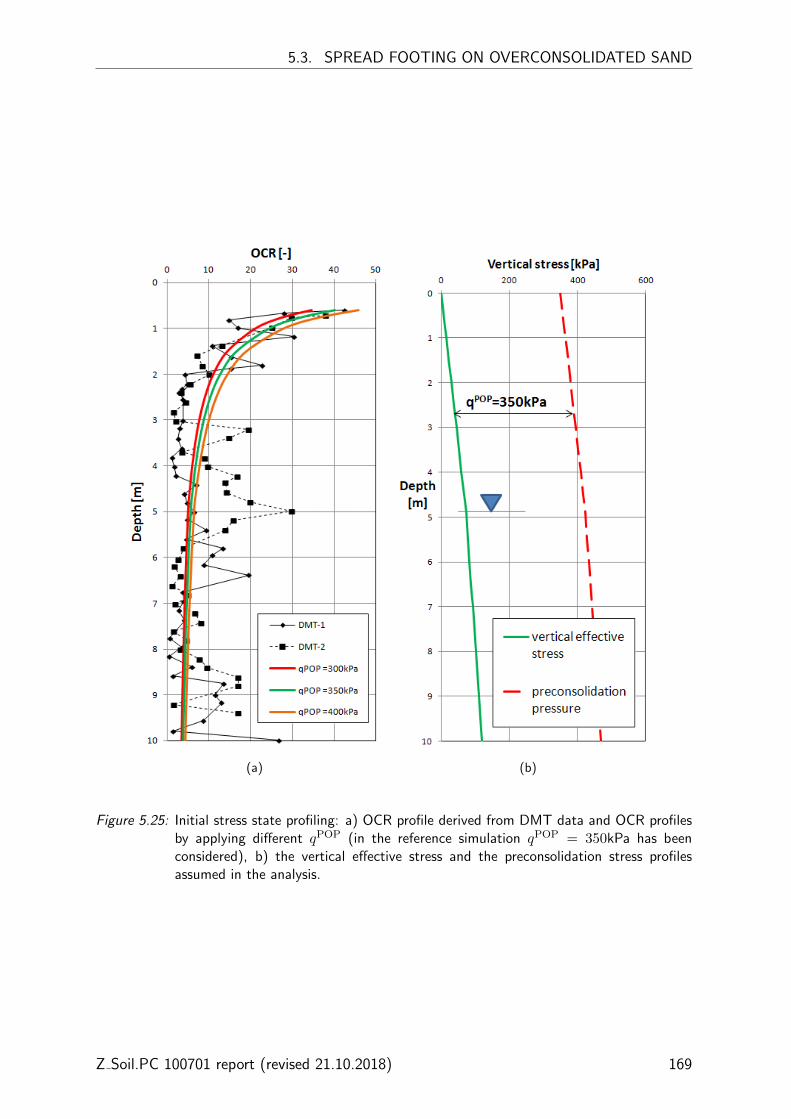
5.3. SPREAD FOOTING ON OVERCONSOLIDATED SAND
(a) (b)
Figure 5.25: Initial stress state profiling: a) OCR profile derived from DMT data and OCR profilesby applying different qPOP (in the reference simulation qPOP = 350kPa has beenconsidered), b) the vertical effective stress and the preconsolidation stress profilesassumed in the analysis.
Z Soil.PC 100701 report (revised 21.10.2018) 169

CHAPTER 5. CASE STUDIES
(a) (b)
Figure 5.26: Dilatometer test data: a) profile of material index ID, b) profile of dilatometer modulusED (both profiles have been used to determine Eur profile based on an empiricalsolution given in Eq.3.25).
170 Z Soil.PC 100701 report (revised 21.10.2018)
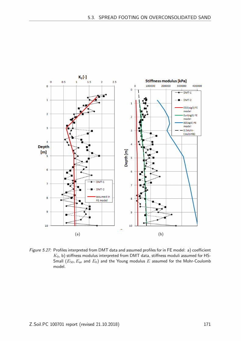
5.3. SPREAD FOOTING ON OVERCONSOLIDATED SAND
(a) (b)
Figure 5.27: Profiles interpreted from DMT data and assumed profiles for in FE model: a) coefficientK0, b) stiffness modulus interpreted from DMT data, stiffness moduli assumed for HS-Small (E50, Eur and E0) and the Young modulus E assumed for the Mohr-Coulombmodel.
Z Soil.PC 100701 report (revised 21.10.2018) 171

CHAPTER 5. CASE STUDIES
Material data. Material data which was assumed for numerical simulation of footing testloading are summarized in Table 5.9.
• Physical properties - taken from the original report (Briaud and Gibbens, 1997)
• Small strain properties - evaluated from the resonant column tests
• Deformation characteristics - E50 derived from triaxial compression test data, and Eur
double-checked with DMT data
• Strength characteristics - derived from triaxial compression test data
• Initial state variables - evaluated from DMT data
Table 5.9: Model parameters used in simulations of the spread footing at Texas site.
Hardening-Soil Mohr-CoulombParameter symbol Unit Sand (triaxial
test)Sand (in situsimulation)
Sand (in situsimulation)
Physical propertiesγD [kN/m3] - 14.9 14.9e0 [-] 0.75 0.75 0.75γ′ [kN/m3] - 9.2 9.2emax [-] 0.91 0.91 0.91
Small strain propertiesE0 [kPa] 260000 380000 -γ0.7 [kN/m3] 0.0002 0.0006 -
Deformation characteristicsEur [kPa] 70000 70000 imposed pro-
file for E:Fig.5.27(b)
E50 [kPa] 16000 16000 -σref [kPa] 100 100 -ν [-] 0.2 0.2 0.3m [-] 0.51 0.51 -
Strength characteristicsφ [o] 36.5 36.5 36.5c [kPa] 3 3 3ψ [o] 1.3 1.3 1.3Rf [-] 0.92 0.92 0.92
Oedometric test characteristicsKNC
0 [-] 0.41 0.41 0.41Eoed [kPa] 20000 10000 10000σref
oed [kPa] 100 100 100
Initial state variablesqPOP [kPa] - 350 -pc0 [kPa] 250 - -K0 (in situ) [-] 1 variable variableKSR
0 [-] 1 0.41 -
172 Z Soil.PC 100701 report (revised 21.10.2018)
5.3. SPREAD FOOTING ON OVERCONSOLIDATED SAND
Numerical simulation of the footing problem. A 3D model of the footing problem whichis shown in Figure 5.28 was considered in the analysis. The 3D mesh can represent a quarterof the real setup thanks to the two symmetry planes. The mesh includes:
• simplified stratigraphy of the subsoil deposits consisting of one sand layer; mesh dimension19.8m×19.8m×17m
• quarter of 3x3m footing which is embedded in the soil at 0.76m and its thickness is equalto 1.22m
• interface between footing faces and soil
• external displacement boundary conditions (BC) (box type)
• pressure BCs which are applied via fluid head and set up along the external boundaries;ground water level is set to 4.9m below soil surface
• nodal force representing a hydraulic jack (due to two symmetry planes the applied nodalis equal to 0.25× F
In addition, Figure 5.29 illustrates how to impose a variable profile of K0 by means of theInitial Stresses option. Note that an existence function is attributed to the superele-ments describing the initial stresses. It means that the effect of imposed initial stress appliesonly to the first analysis step, i.e. during the generation of the initial state. This interventionis needed to avoid imposing soil’s initial stress onto the material which replaces excavated soil.
Analysis details
• analysis type: 3D deformation+flow
• driver type: steady state
• constitutive models:
F Sand: three variants: (i) HS-Standard, (ii) HS-SmallStrain, (iii) Standard Mohr-Coulomb
F Footing: elastic material E = 20GPa, ν = 0.2
The following stages are considered in the model:
1. Generating an initial stress state for an assumed K in situ0 in sand layer and initial pore
pressure BC
2. Installation of the quadratic footing with simultaneous replacement of soil’s material in theembedded part of footing
3. Gradual application of test load at the quadratic footing
Z Soil.PC 100701 report (revised 21.10.2018) 173

CHAPTER 5. CASE STUDIES
Figure 5.28: 3D mesh representing a quarter of 3x3m footing.
Figure 5.29: Imposing a variable K0 profile by means of the Initial Stresses option.
174 Z Soil.PC 100701 report (revised 21.10.2018)
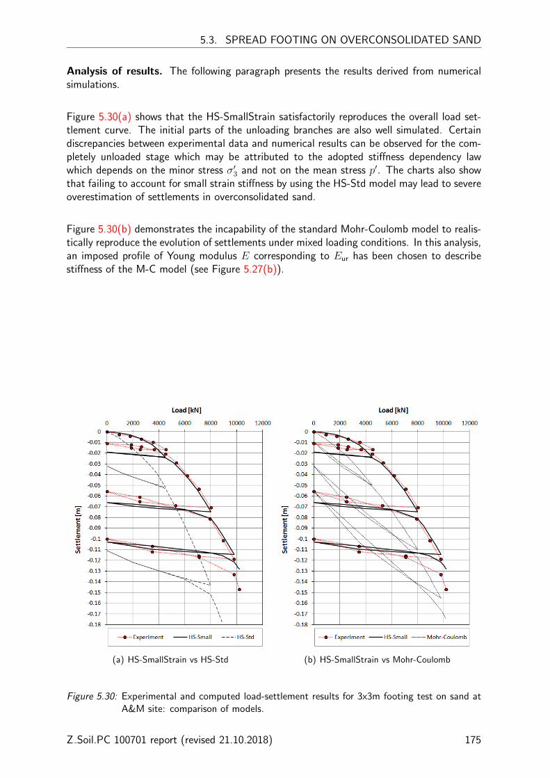
5.3. SPREAD FOOTING ON OVERCONSOLIDATED SAND
Analysis of results. The following paragraph presents the results derived from numericalsimulations.
Figure 5.30(a) shows that the HS-SmallStrain satisfactorily reproduces the overall load set-tlement curve. The initial parts of the unloading branches are also well simulated. Certaindiscrepancies between experimental data and numerical results can be observed for the com-pletely unloaded stage which may be attributed to the adopted stiffness dependency lawwhich depends on the minor stress σ′3 and not on the mean stress p′. The charts also showthat failing to account for small strain stiffness by using the HS-Std model may lead to severeoverestimation of settlements in overconsolidated sand.
Figure 5.30(b) demonstrates the incapability of the standard Mohr-Coulomb model to realis-tically reproduce the evolution of settlements under mixed loading conditions. In this analysis,an imposed profile of Young modulus E corresponding to Eur has been chosen to describestiffness of the M-C model (see Figure 5.27(b)).
(a) HS-SmallStrain vs HS-Std (b) HS-SmallStrain vs Mohr-Coulomb
Figure 5.30: Experimental and computed load-settlement results for 3x3m footing test on sand atA&M site: comparison of models.
Z Soil.PC 100701 report (revised 21.10.2018) 175

CHAPTER 5. CASE STUDIES
(a) HS-SmallStrain: sensitivity to E0 (b) HS-SmallStrain: sensitivity to γ0.7
Figure 5.31: Experimental and computed load-settlement results for 3x3m footing test on sand atA&M site: sensitivity to small-strain stiffness parameters.
Figure 5.31(a) demonstrates sensitivity of HS-SmallStain to E0. It can be noticed that un-derestimating small-strain stiffness may lead to an overestimation of settlements, affectingespecially the initial part of the load-settlement curve. Hence, by comparing the results forunderestimated small-stiffness and the curve derived for HS-Std (small-strain stiffness inac-tive), it can be concluded that it is better to run a simulation with underestimatedsmall-strain parameters than not to account for the small-strain stiffness at all.
Figure 5.31(b) illustrates the sensitivity of HS-SmallStain to the small-strain threshold param-eter γ0.7. It can be noticed that the lower value of this parameter allows an earlier degradationof small-strain stiffness.
176 Z Soil.PC 100701 report (revised 21.10.2018)

5.3. SPREAD FOOTING ON OVERCONSOLIDATED SAND
(a) HS-SmallStrain: Overconsolidated vs normally-consolidated sand
(b) HS-SmallStrain: Overconsolidated sand throughqPOP (variable) vs OCR = 10 (constant)
Figure 5.32: Experimental and computed load-settlement results for 3x3m footing test on sand atA&M site: sensitivity to the initial stress history setup.
Figure 5.32(a) shows an example of settlement overestimation if the simulation is carried outnot accounting for the preconsolidation effect in the overconsolidated sand. In this particularexample, assuming that the soil is normally-consolidated leads to a severe settlement over-estimation of 270% for the first portion of loading (up to 4500kN) and maximal settlementsachieved during the load test are doubled compared to the reference simulation for the over-consolidated material.
Figure 5.32(b) compares two analyzes for the overconsolidated sand (i) with variable OCRprofile obtained with qPOP = 350kPa, and (ii) with an equivalent OCR = 10 as an ”aver-aged” value between 0.5m and 5m. No difference between numerical curves can be observedbetween 0kN and 2500kN as small-strain stiffness has not been degraded yet. The differ-ence starts to occur at the magnitude of load from 2500kN to 8000kN. This is due to anunderestimation of the preconsolidation pressure in the upper part of subsoil for a case withconstant OCR = 10. In this case, an earlier activation of the cap mechanism yields in largervolumetric strains below the footing. The curves start to overlap each other for loads from8000kN to 10000kN as the zone of the load influence expands below the footing. A furtherincrease of load would show larger settlements for the case with the variable OCR as thezone of influence includes depth levels of lower OCR values.
Z Soil.PC 100701 report (revised 21.10.2018) 177

CHAPTER 5. CASE STUDIES
(a) HS-SmallStrain: sensitivity to initial stress setup (b) HS-SmallStrain: sensitivity to qPOP
Figure 5.33: Experimental and computed load-settlement results for 3x3m footing test on sand atA&M site: sensitivity to the initial stress setup.
Figure 5.33(a) illustrates the sensitivity of numerical predictions to the initial setup of thecoefficient of earth pressure ”at rest”. In the reference simulation, the profile of K0 for over-consolidated soil has been evaluated by means of the Marchetti’s dilatometer test (DMT),whereas in the second simulation a constant profile of K0 equal to KNC
0 = 1 − sin(φ) hasbeen assumed. This analysis reveals slightly larger settlements for KNC
0 = 0.41 which is at-tributed to lower initial soil stiffness. Note that soil stiffness in the HS model depends on theminor effective stress so in the case where K0 = KNC
0 the initial stiffness is defined by σ′h0,whereas for the reference simulation, the initial soil stiffness is defined by σ′v0 up to around2.2m as K0 > 1. The user should be aware that soil stiffness in the HS model evolves duringsimulation with amplitudes of stress level.
Finally, Figure 5.33(b) reveals the sensitivity of a numerical simulation to the initial precon-solidation setup. The chart presents numerical predictions for three qPOP values: 350kPa(reference simulation), 300kPa and 400kPa. The sensitivity of the OCR profile to the speci-fied values of qPOP is presented in Figure 5.25(a).
178 Z Soil.PC 100701 report (revised 21.10.2018)
Appendix A
Determination of undrained shearstrength
A.1 Non-uniqueness of undrained shear strength
It has been widely recognized that the in situ behavior of soils may be significantly differentfrom that of laboratory samples. This can be mainly attributed to the quality of the intactspecimens which may depend on drilling and sampling methods and sample geometry (DeG-root and Sandven, 2004). The disturbance of samples may increase during their insertion intoa sampling tube, transportation, relaxation of stresses, drying, temperature changes, trimmingand, finally, their installation in the testing cells, etc. (Hight et al., 1992). Different samplingdevices such as piston samplers, thin walled tubes or downhole block samplers can providespecimens for which different magnitudes of preconsolidation pressure or undrained shearstrength su are measured (e.g. Hight et al., 1992; Tanaka and Tanaka, 1999). Experienceshows that sample disturbance may lead to underestimation of the apparent preconsolidationpressure or undrained shear strength (Karlsrud, 1999; Fioravante, 2004).Inconsistencies in su values measured by laboratory and field tests may also stem from thenon-uniqueness of this property. The undrained shear strength su is not a unique soil pa-rameter (Wroth, 1984; Jamiolkowski et al., 1985), as it depends on the type of test, whichinvolves particular strain paths (cf. Figure A.1).
The differences in interpreted results also stems from the time-dependent behavior of soils(e.g. Vaid and Campanella, 1977; Leroueil, 1988; Sheahan et al., 1996; Penumadu et al.,1998). The undrained shear strength increases linearly with the logarithm of the shear strain(Bjerrum, 1972; Nakase and Kamei, 1986). For instance, the testing speed for SBPT orCPTU can be one or more orders of magnitude greater than that used in the triaxial com-pression test TC (ε = 0.01%/min), see Figure A.2. Laboratory tests with the use of a modelpressuremeter in clays have revealed an increase of su of about 10% for every tenfold increaseof strain rate (Prapaharan et al., 1989). While the overstimation of su derived from pres-suremeter test due to the strain rate effect can be reasonably small, in the order of 10-20%,the differences for CPTU can be much larger. The extrapolated results of Bjerrum (1972)(Figure A.2) can indicate that neglecting the strain effect in the analysis of penetration maylead to the considerable overestimation of su of about 40% with respect to the value obtainedfor the conventional triaxial compression. Since the undrained shear strength is a function ofthe stress history, the similar effects can be observed for the derived values of preconsolida-tion pressure σ′p. The study carried out by Leroueil et al. (1983b) revealed the increase of

APPENDIX A. DETERMINATION OF UNDRAINED SHEAR STRENGTH
(a) (b)
Figure A.1: Undrained shear strength in normally consolidated soil (a) as a function of shear modesfor various tests: triaxial undrained compression tests (CIUC and CK0UC), plain straincompression test (PSC), direct simple shear test (DSS) and field vane test (FVT) (afterWroth, 1984), (b) profiles for field and laboratory tests on Onsøy clay (from Lacasseet al., 1981).
.
about 10-14% for σ′p per log cycle of volumetric strain rate εv in the constant rate of strainoedometer test (CRS).
10−3
10−2
10−1
100
101
102
103
0.8
0.9
1
1.1
1.2
1.3
1.4
1.5
Strain Rate, ε [%/min]
c u/ c
u,0.
01
Nakase & Kamei (1986) CKoUC
Penu
mad
u et
al.(
1998
) PSC
Bjerrum (1
972) CK o
UC
extrapolated
TC
SB
PT
CP
TU
M10M15M30
Vaid & Campanella(1977) CIUC
Prapaharan et al.(1989)PMT
TESTSTRAIN
RATE
Figure A.2: The strain rate effect on undrained shear strength su for different shear modes anda schematic comparison of test strain rates for triaxial compression (TC), self-boringpressuremeter (SBPT) and piezocone (CPTU).
180 Z Soil.PC 100701 report (revised 21.10.2018)

A.2. DETERMINATION OF SU FROM FIELD TESTS
A.2 Determination of su from field tests
FVT. The interpretation of su from the standardly used field vane test (see Figure A.3) canbe carried out with the conventional formula:
su =6M
7πD3= 0.2728
M
D3(A.1)
in which M is the maximum recorded torque, and D is the diameter of vane.Since the values of su obtained with the above equation can be too conservative, Chandler(1988) suggested increasing the factor 0.2728 to 0.2897.
Figure A.3: Standard dimensions of the most commonly used field vane test (from Chandler, 1988).
DMT. The values of su can be correlated with the Marchetti’s dilatometer data through theoriginal formula suggested by Marchetti (1980):
su = 0.22σ′v0(0.5KD)1.25 (A.2)
where KD is the horizontal stress index which is calculated based on the first dilatometerreading p0 (KD = (p0 − u0)/σ′v0).
Z Soil.PC 100701 report (revised 21.10.2018) 181

APPENDIX A. DETERMINATION OF UNDRAINED SHEAR STRENGTH
182 Z Soil.PC 100701 report (revised 21.10.2018)

Appendix B
Estimation of compression index
Table B.1: Some correlation equations for estimating consolidation parameters (after Holtz et al.,1986; Bowles, 1997; Kempfert, 2006).
Compression index Applicability Reference
Cc = 0.009(wL − 10) Normally consolidated claysof low to medium sensitivityand wL < 100(±30% er-ror)
Terzaghi and Peck(1967)
Cc = 0.141Gs(γSAT/γD) All clays Rendon-Herrero(1983)
Cc = 0.141G1.2s [(1 + e0)/Gs]
2.38 All clays (94 data points) Rendon-Herrero(1983)
Cc = 1.15(e0 − 0.35) All clays, uniformly packed Nishida (1956)Cc = 1.15(e− 0.91) All clays, loosely packed
e > 0.9Nishida (1956)
Cc = 0.009wn + 0.005wL All clays Koppula (1986)Cc = 0.00234wLGs All inorganic clays Nagaraj and Murthy
(1985)Cc = 0.37(e0 + 0.003wL + 0.0004wn − 0.34) 678 data points Azzouz et al. (1976)Cc = 0.00917(wL − 13) 56 data points Mayne (1980)Cc = −0.156 + 0.411e+ 0.00058wL 72 data points Al-Khafaji and An-
dersland (1992)Cc = 0.156e+ 0.0107 Remoulded all clays Azzouz et al. (1976)Cc = 0.208e+ 0.0083 Chicago clays Azzouz et al. (1976)Cc = 0.007(wL − 10) Remoulded clays Skempton (1944)Cc = 0.007(wL − 7) Remoulded clays Azzouz et al. (1976)Cc = 0.005GsIP Remoulded clays Wroth and Wood
(1978)Cc = 0.5(IP /100)Gs Remoulded clays Wroth and Wood
(1978)Cc = 0.046 + 0.0104IP Best for IP < 50% Nakase (1988)Cc = 1.15e Deformable but incom-
pressible soilNishida (1956)
Cc = 0.0115wn Organic soils - meadowmats, peats, and organicsilt and clay
Azzouz et al. (1976)
Cc = 0.75(e0 − 0.50) Soils with low plasticity Azzouz et al. (1976)Cc = 0.30(e0 − 0.27) Inorganic silty sand-silty
clayHough (1969)
Cc = PI/74 Data from different soils Kulhawy and Mayne(1990)

APPENDIX B. ESTIMATION OF COMPRESSION INDEX
Cc = 0.0093wn Chicago clays and AlbertaProvince in Canada (109data points)
Koppula (1981)
Cc = 17.66/100000w2n + 0.00593wn − 0.135 Chicago clays Azzouz et al. (1976)
Cc = 0.015(wn − 8) Soils in Taipei Moh et al. (1989)Cc = 0.54(e− 0.23) Soils in Taipei Moh et al. (1989)Cc = 0.0046(wL − 9) Brazilian clays Azzouz et al. (1976)Cc = 1.21 + 1.005(e− 1.87) Motley clays from Sao
PauloAzzouz et al. (1976)
Cc = 0.0037(wL + 25.5) Cincinnati and NorthernKentucky
Dayal (2006)
Cc = 0.0135wn − 0.1169 Cincinnati and NorthernKentucky
Dayal (2006)
Cc = 0.0042IP + 0.165 Cincinnati and NorthernKentucky
Dayal (2006)
Cc = 0.46e− 0.049Gs + 0.0023 Cincinnati and NorthernKentucky
Dayal (2006)
Cc = 0.4965e− 0.0014wn − 0.123 Cincinnati and NorthernKentucky
Dayal (2006)
Cc = −0.247e+ 0.004wL + 0.01wn + 0.021 Cincinnati and NorthernKentucky
Dayal (2006)
Cc = 0.0018/(1− 0.0109n) Remoulded clays in Japan(Ariake)
Park and Koumoto(2004)
Cc = 0.00269/(1− 0.0115n) Undisturbed clays in Japan(Ariake)
Park and Koumoto(2004)
Cc = 0.02 + 0.014IP North Atlantic clays Nacci et al. (1975)Cc = 0.02 + 0.014IP North Atlantic clays Nacci et al. (1975)Cc = 0.011(wL − 6.36) East coast of Korea Yoon et al. (2004)Cc = 0.01(wn + 2.83) East coast of Korea Yoon et al. (2004)Cc = 0.39(e− 0.13) East coast of Korea Yoon et al. (2004)Cc = −0.16γD + 2.4 East coast of Korea Yoon et al. (2004)Cc = 0.0098wn + 0.194e− 0.0025IP − 0.256 East coast of Korea Yoon et al. (2004)Cc = 0.012(wL + 16.4) South coast of Korea Yoon et al. (2004)Cc = 0.013(wn − 3.85) South coast of Korea Yoon et al. (2004)Cc = 0.54(e− 0.37) South coast of Korea Yoon et al. (2004)Cc = −0.0003wn + 0.538e+ 0.002wL − 0.3 South coast of Korea Yoon et al. (2004)Cc = 0.165 + 0.01IP South coast of Korea Yoon et al. (2004)Cc = 0.01(wL − 10.9) West coast of Korea Yoon et al. (2004)Cc = 0.011(wn − 11.22) West coast of Korea Yoon et al. (2004)Cc = 0.37(e− 0.28) West coast of Korea Yoon et al. (2004)Cc = −0.066γD + 1.15 West coast of Korea Yoon et al. (2004)Cc = 0.0038wn + 0.12e+ 0.0065wL − 0.248 West coast of Korea Yoon et al. (2004)
184 Z Soil.PC 100701 report (revised 21.10.2018)
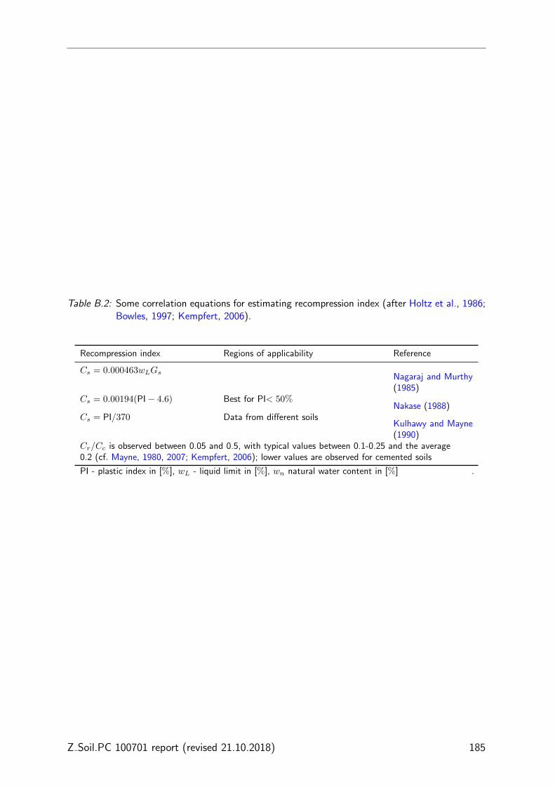
Table B.2: Some correlation equations for estimating recompression index (after Holtz et al., 1986;Bowles, 1997; Kempfert, 2006).
Recompression index Regions of applicability Reference
Cs = 0.000463wLGsNagaraj and Murthy(1985)
Cs = 0.00194(PI− 4.6) Best for PI< 50%Nakase (1988)
Cs = PI/370 Data from different soilsKulhawy and Mayne(1990)
Cr/Cc is observed between 0.05 and 0.5, with typical values between 0.1-0.25 and the average0.2 (cf. Mayne, 1980, 2007; Kempfert, 2006); lower values are observed for cemented soils
PI - plastic index in [%], wL - liquid limit in [%], wn natural water content in [%] .
Z Soil.PC 100701 report (revised 21.10.2018) 185
APPENDIX B. ESTIMATION OF COMPRESSION INDEX
186 Z Soil.PC 100701 report (revised 21.10.2018)

Appendix C
Estimation of shear wave velocity
Table C.1: Typical values of shear wave velocity and density for different geomaterials (afterLavergne, 1986).
Shear wave velocity Dry unit weightVs [m/s] γ [g/cm3]
Soil type Min Max Min Max
Screes, organic topsoil 100 300 1.7 2.4Dry sands 100 500 1.5 1.7Wet sands 400 1200 1.9 2.1Clays 200 800 2.0 2.4Marls 750 1500 2.1 2.6Sandstones 1200 2800 2.1 2.4Lime stones 2000 3300 2.4 2.7Chalk 1100 1300 1.8 2.3Salt 2500 3100 2.1 2.3Anhydrite 2200 3100 2.9 3.0Dolomite 1900 3600 2.5 2.9Granite 2500 3300 2.5 2.7Basalte 2800 3400 2.7 3.1Carbon 1000 1400 1.3 1.8Ice 1700 1900 0.9 0.9
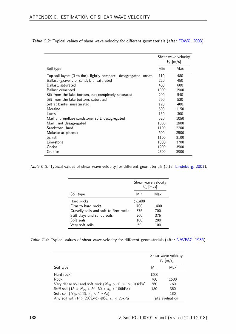
APPENDIX C. ESTIMATION OF SHEAR WAVE VELOCITY
Table C.2: Typical values of shear wave velocity for different geomaterials (after FOWG, 2003).
Shear wave velocityVs [m/s]
Soil type Min Max
Top soil layers (3 to 6m), lightly compact., desagregated, unsat. 110 480Ballast (gravelly or sandy), unsaturated 220 450Ballast, saturated 400 600Ballast cemented 1000 1500Silt from the lake bottom, not completely saturated 290 540Silt from the lake bottom, saturated 390 530Silt at banks, unsaturated 120 400Moraine 500 1150Loess 150 300Marl and mollase sandstone, soft, desagregated 520 1050Marl , not desagregated 1000 1900Sandstone, hard 1100 2200Molasse at plateau 600 2500Schist 1100 3100Limestone 1800 3700Gneiss 1900 3500Granite 2500 3900
Table C.3: Typical values of shear wave velocity for different geomaterials (after Lindeburg, 2001).
Shear wave velocityVs [m/s]
Soil type Min Max
Hard rocks >1400Firm to hard rocks 700 1400Gravelly soils and soft to firm rocks 375 700Stiff clays and sandy soils 200 375Soft soils 100 200Very soft soils 50 100
Table C.4: Typical values of shear wave velocity for different geomaterials (after NAVFAC, 1986).
Shear wave velocityVs [m/s]
Soil type Min Max
Hard rock 1500Rock 760 1500Very dense soil and soft rock (N60 > 50, su > 100kPa) 360 760Stiff soil (15 > N60 < 50, 50 < su < 100kPa) 180 360Soft soil (N60 < 15, su < 50kPa) 180Any soil with PI> 20%,w> 40%, su < 25kPa site eveluation
188 Z Soil.PC 100701 report (revised 21.10.2018)

SPT. Most published correlations for SPT are based on uncorrected N-values. These corre-lations are given in:
• for all soil types: Table C.5 (insight prrovided in C.1),
• for sands: Table C.6 (Figure C.2),
• for silts: Table C.7 (Figure C.3),
• for clays: Table C.8 (Figure C.4).
Table C.5: SPT-Based correlations for all type of soils.
Reference Country Soil Type Equation Correlationcoeffi-cient
Ohba & Toriumi (1970)1 Japan Alluvium Vs = 84N0.3160 –
Fujiwara (1972)2 Japan – Vs = 92.1N0.33760 –
Ohsaki & Iwasaki (1973)1 Japan – Vs = 81.3N0.3960 0.886
Imai and Yoshimura(1975)
Japan – Vs = 76N0.33360 –
Imai (1977)2 Japan Quaternary and Pleis-tocene Alluvium
Vs = 91N0.33760 –
Ohta and Goto (1978)Japan Quaternary and Pleis-
tocene AlluviumVs = 85.34N0.348
60 0.719
Imai & Tonouchi (1982)1 Japan – Vs = 97N0.31460 0.868
Seed et al. (1983)– – Vs = 56N0.5
60 –
Jinan (1987)Shanghai Soft Holocene Deposits Vs = 116.1(N60 +
0.3185)0.2020.7
Athanasopoulos (1995)Greece – Vs = 107.6N0.36
60 –
Sisman (1995)2 – – Vs = 32.8N0.5160 –
Iyisan (1996)2 – – Vs = 51.5N0.51660 –
Kiku et al. (2001)2 Turkey – Vs = 68.3N0.29260 –
Hasancebi and Ulusay(2007)
Turkey Quaternary Alluviumand Detritus
Vs = 90N0.30860 0.73
1 Referenced by Sykora (1987)2 Referenced by Hasancebi and Ulusay (2007)
Z Soil.PC 100701 report (revised 21.10.2018) 189

APPENDIX C. ESTIMATION OF SHEAR WAVE VELOCITY
Table C.6: SPT-Based correlations for sands.
Reference Country Soil Type Equation Correlationcoeffi-cient
Shibata (1970)– – Vs = 31.7N0.54
60 –
Ohta et al. (1972)Japan – Vs = 87.2N0.36
60 –
Imai (1977)2 Japan Quaternary and Pleis-tocene Alluvium
Vs = 80.6N0.33160 –
Ohta & Goto (1978b)1 Japan Quaternary and Pleis-tocene Alluvium
Vs = 88.4N0.33360 0.719
Imai & Tonouchi (1982)1 Japan Quaternary and Pleis-tocene Alluvium
Vs = 87.8N0.31460 0.69
Sykora & Stokoe (1983)1 – – Vs = 100.5N0.2960 0.84
Okamoto et al. (1989)Japan – Vs = 125N0.3
60 –
Lee (1990)Taiwan – Vs = 57.4N0.49
60 0.62
Lee (1992)Taiwan – Vs = 157.13 + 4.74N60 0.691
Pitilakis et al. (1999)Greece Alluvium Vs = 145N0.178
60 0.70
Hasancebi and Ulusay(2007)
Turkey Quaternary Alluviumand Detritus
Vs = 90.82N0.31960 0.65
Dikmen (2009)WesterncentralAnatolia,Turkey
– Vs = 73N0.3360 –
1 Referenced by Sykora (1987)2 Referenced by Hasancebi and Ulusay (2007)
Table C.7: SPT-Based correlations for silts.
Reference Country Soil Type Equation Correlationcoeffi-cient
Lee (1990)Taiwan – Vs = 105.64N0.32
60 0.73
Lee (1992)Taiwan – Vs = 103.99(N60 + 1)0.334 0.798
Pitilakis et al. (1999)Greece Alluvium Vs = 145N0.178
60 0.70
Dikmen (2009)WesterncentralAnatolia,Turkey
– Vs = 60N0.3660 –
190 Z Soil.PC 100701 report (revised 21.10.2018)
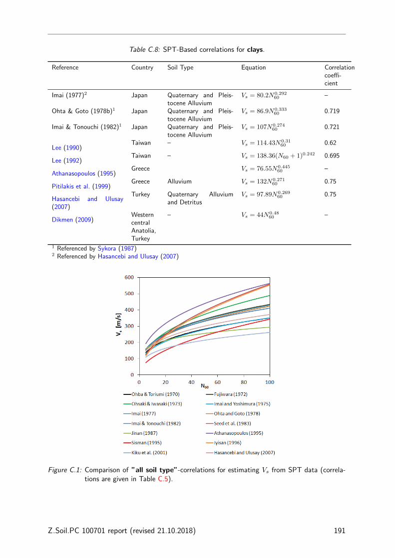
Table C.8: SPT-Based correlations for clays.
Reference Country Soil Type Equation Correlationcoeffi-cient
Imai (1977)2 Japan Quaternary and Pleis-tocene Alluvium
Vs = 80.2N0.29260 –
Ohta & Goto (1978b)1 Japan Quaternary and Pleis-tocene Alluvium
Vs = 86.9N0.33360 0.719
Imai & Tonouchi (1982)1 Japan Quaternary and Pleis-tocene Alluvium
Vs = 107N0.27460 0.721
Lee (1990)Taiwan – Vs = 114.43N0.31
60 0.62
Lee (1992)Taiwan – Vs = 138.36(N60 + 1)0.242 0.695
Athanasopoulos (1995)Greece Vs = 76.55N0.445
60 –
Pitilakis et al. (1999)Greece Alluvium Vs = 132N0.271
60 0.75
Hasancebi and Ulusay(2007)
Turkey Quaternary Alluviumand Detritus
Vs = 97.89N0.26960 0.75
Dikmen (2009)WesterncentralAnatolia,Turkey
– Vs = 44N0.4860 –
1 Referenced by Sykora (1987)2 Referenced by Hasancebi and Ulusay (2007)
Figure C.1: Comparison of ”all soil type”-correlations for estimating Vs from SPT data (correla-tions are given in Table C.5).
Z Soil.PC 100701 report (revised 21.10.2018) 191
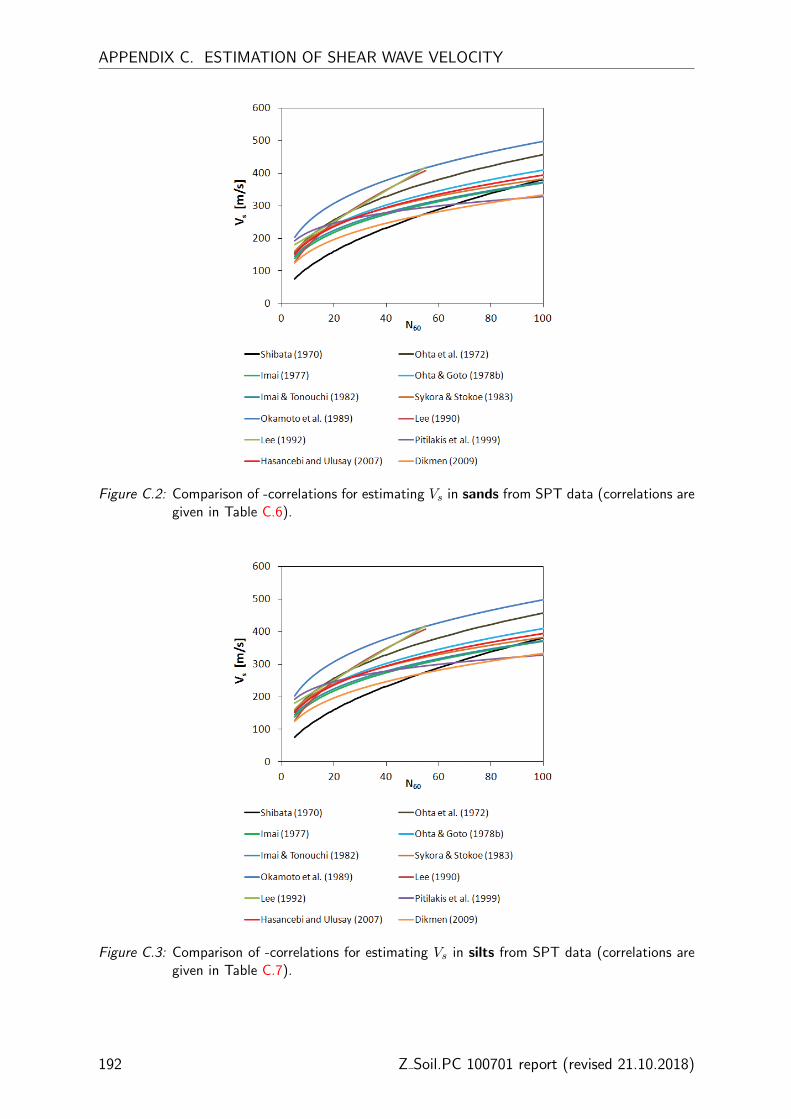
APPENDIX C. ESTIMATION OF SHEAR WAVE VELOCITY
Figure C.2: Comparison of -correlations for estimating Vs in sands from SPT data (correlations aregiven in Table C.6).
Figure C.3: Comparison of -correlations for estimating Vs in silts from SPT data (correlations aregiven in Table C.7).
192 Z Soil.PC 100701 report (revised 21.10.2018)

Figure C.4: Comparison of -correlations for estimating Vs in clays from SPT data (correlations aregiven in Table C.8).
CPT. A number of correlations can be used to estimate shear wave velocity based on CPTdata. Correlations were developed for a generic soil types: Table C.9, for sands: Table C.10,for clays: Table C.11. Graphical comparisons of these correlations are presented in Figure forsands
Table C.9: CPT-based correlations for all soil types.
Reference Soil Type Vs [m/s] Remarks
Hegazy and Mayne (1995)sands, silts,clays, mixedsoil types
(10.1 log qt − 11.4)1.67(fs/qt · 100)0.3 qt, fs in kPa
Mayne (2006a)saturatedclays, silts,and sands
118.8 log fs + 18.5 fs in kPa
Table C.10: CPT-based correlations for sands.
Reference Soil Type Vs [m/s] Remarks
Baldi et al. (1989)Giola Taura Sand w/Gravel,Po River sands
277q0.13t σ′0.27v0 qt, σ′v0 in MPa
Hegazy and Mayne (1995)– 13.18q0.192t σ′0.179v0 qt, σ
′v0 in kPa
Hegazy and Mayne (1995)– 12.02q0.319t f−0.0466s qt, fs in kPa
Z Soil.PC 100701 report (revised 21.10.2018) 193
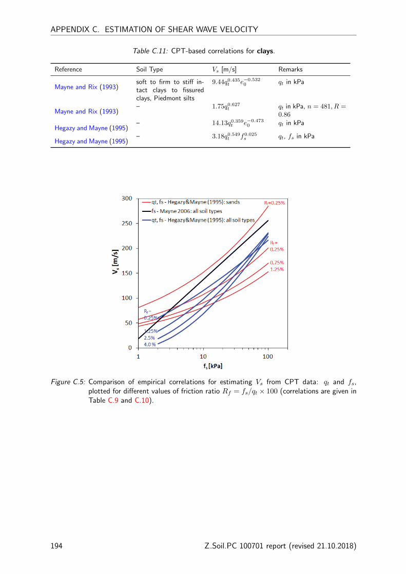
APPENDIX C. ESTIMATION OF SHEAR WAVE VELOCITY
Table C.11: CPT-based correlations for clays.
Reference Soil Type Vs [m/s] Remarks
Mayne and Rix (1993)soft to firm to stiff in-tact clays to fissuredclays, Piedmont silts
9.44q0.435t e−0.5320 qt in kPa
Mayne and Rix (1993)– 1.75q0.627t qt in kPa, n = 481, R =
0.86
Hegazy and Mayne (1995)– 14.13q0.359t e−0.4730 qt in kPa
Hegazy and Mayne (1995)– 3.18q0.549t f0.025s qt, fs in kPa
Figure C.5: Comparison of empirical correlations for estimating Vs from CPT data: qt and fs,plotted for different values of friction ratio Rf = fs/qt × 100 (correlations are given inTable C.9 and C.10).
194 Z Soil.PC 100701 report (revised 21.10.2018)
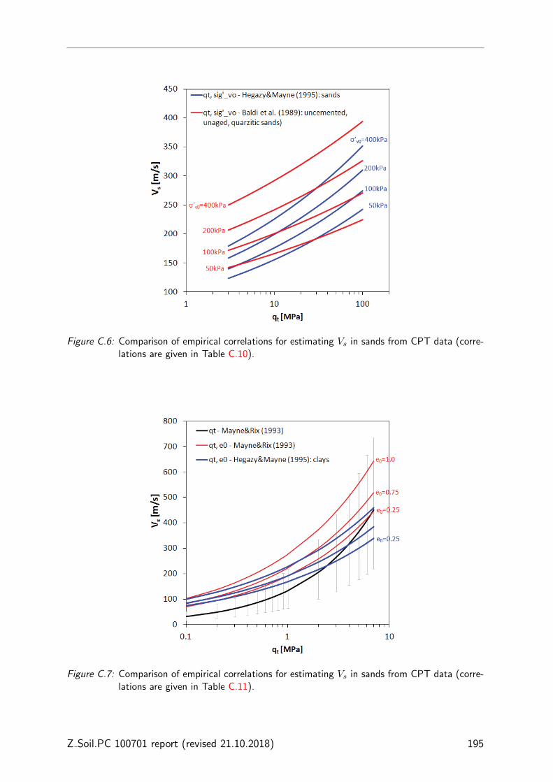
Figure C.6: Comparison of empirical correlations for estimating Vs in sands from CPT data (corre-lations are given in Table C.10).
Figure C.7: Comparison of empirical correlations for estimating Vs in sands from CPT data (corre-lations are given in Table C.11).
Z Soil.PC 100701 report (revised 21.10.2018) 195


References
References
Addenbrooke, T., Potts, D., and Puzrin, A. (1997). The influence of pre-failure soil stiffness on the numericalanalysis of the tunnel construction. Geotechnique, 47(3):693–712. 4, 145, 148
Al-Khafaji, A. and Andersland, O. (1992). Equations for compression index approximation. J Geotech EngASCE, 118(1):148–153. 183
Alpan, I. (1970). The geotechnical properties of soils. Earth-Science Reviews, 6:5–49. 62, 95
Amar, S., Clarke, B., Gambin, M., and Orr, T., editors (1991). The application of pressuremeter test resultsto foundation design in Europe. Part 1: Predrilled pressuremeters/self-boring pressuremeters. Balkema,Rotterdam. 121
Athanasopoulos, G. A. (1995). Empirical correlations vs-nspt for soils of greece: a comparative study ofreliability. In Cakmak, A., editor, 7th Int Conf on Soil Dynamics and Earthquake Engineering, pages19–36, Chania, Crete. 189, 191
Atkinson, J. and Sallfors, G. (1991). Experimental determination of soil properties. In Proc. 10th ECSMFE,volume 3, pages 915–956, Florence, Italy. 2
Azzouz, A., Krizek, R., and Corotis, R. (1976). Regression analysis of soil compressibility. Soils and Founda-tions, 16(2):19–29. 183, 184
Baldi, G., Bellotti, R., Ghionna, V., Jamiolkowski, M., and Lo Presti, D. (1989). Modulus of sands fromcpts and dmts. In Proc. 12th International Conference on Soil Mechanics and Foundation Engineering,volume 1, pages 165–170, Rio de Janeiro, Brazil. Balkema, Rotterdam. 193
Baldi, G., Bellotti, R., Ghionna, V., Jamiolkowski, M., Marchetti, S., and Pasqualini, E. (1986). Flatdilatometer tests in calibration chambers. In In Situ 86, ASCE Spec. Conf. on ”Use of In Situ Tests inGeotechn Engineering”, volume GSP 6, pages 431–436. ASCE. 65, 91
Begemann, H. (1974). General report for central and western europe. In European Symp. on PenetrationTesting, Stockholm, Sweden. 74
Belotti, R., Ghionna, V., Jamiolkowski, M., Lancellotta, R., and Manfredini, G. (1986). Deformation charac-teristics of cohesionless soisl in in situ tests. In ASCE, editor, In Situ 86, Geotechnical Special Publications,pages 47–73, New York. ASCE. 65
Benz, T. (2007). Small-strain stiffness of soils and its numerical consequences. Phd, Universitat Sttutgart.7, 11, 61, 80, 117, 129, 130, 131, 132, 137
Biarez, J. and Hicher, P. (1994). Elementary mechanics of soil behaviour. Saturated remoulded soils. Balkema,Rotterdam. 59, 60, 92, 94
Bjerrum, L. (1972). Embankments on soft ground. In Proc. Am.Soc. Civ Engs Specialty Conf. on Perfomenceof Earth and Earth supported Structures., volume 2, pages 1–54, Perdue University. 179
Bolton, M. (1986). The strength and dilatancy of sands. Geotechnique, 36(1):65–78. 86
Bowles, J. (1997). Foundation analysis and design. McGraw-Hill. 7, 74, 81, 83, 118, 183, 185
References
Briaud, J.-L. and Gibbens, R. (1997). Large scale load test and data base of spread footings on sand.Technical Report Publication No. FHWA RD-97-068, Texas A&M University. 161, 172
Brinch Hansen, J. and Lundgren, H., editors (1958). Geoteknik. Teknisk Forlag, Kopenhagen. 81
Carter, M. and Bentley, S. (1991). Correlations of soil properties. Penetech Press Publishers, London. 85,102
Casagrande, A. (1936). The determination of the pre-consolidation load and its practical significance. InCasagrande, A., editor, In Proc. 1st Int Soil Mech and Found Engng Conf, 22-26 June 1936, volume 3,pages 60–64, Cambridge, Mass. Graduate School of Engineering, Harvard University, Cambridge, Mass.49
Chandler, R. (1988). The in-situ measurements of the undrained shear strength of clays using the field tests.Technical report, ASTM. 181
Chaudary, S., Kuwano, J., and Hayano, Y. (2004). Measurement of quasi-elastic stiffness parameters ofdense toyoura sand in hollow cylinder apparatus and triaxial apparatus with bender elements. GeotechnicalTesting Journal, 27(1):1–13. 60, 80
Chen, B. and Mayne, P. (1994). Profiling the OCR of clays by piezocone tests. Technical Report Rep. No.CEEGEO-94-1, Georgia Institute of Technology. 119
Chen, B. and Mayne, P. (1996). Statistical relationships between piezocone measurements and stress historyof clays. Can Geotech J, 33:488–498. 119
Clough, G., Briauld, J., and Hughes, J. (1990). The developement of prssuremeter testing. In Pressuremeters,3rd Int Symp on Pressuremeters, pages 25–45, Oxford. Thomas Telford, London. 121
Dalton, J. and Hawkins, P. (1982). Fields of stress - some measurements of the in-situ stress in a meadowin the Cambridgeshire countryside. Ground Engineering, 15(4):15–23. 121
D’Appolonia, D., D’Appolonia, E., and Brissette, R. (1970). Closure: Settlement of spread footing on sand.J Soils Mechanics and Foundation Division ASCE, 96(2):754–762. 74
Darendeli, M. (2001). Development of a New Family of Normalized Modulus Reduction and Material DampingCurves. PhD thesis, University of Texas. 70, 100
Darendeli, M. and Stokoe, K. (2001). Development of a new family of normalized modulus reduction andmaterial damping curves. Technical report, University of Texas. 68, 69
Das, B. (2008). Advanced Soil Mechanics. Taylor & Francis, London & New York. 88, 89
Dayal, I. (2006). Consolidation analyses of greater cincinnati soils. MSc. Technical report, University ofCincinnati. 184
DeGroot, D. and Sandven, R. (2004). General report: Laboratory and field comparisons. In de Fonseca, V.and Mayne, editors, Proc. ISC-2 on Geotechnical and Geophysical Site Characterization, pages 1775–1789,Porto, Portugal. Millpress, Rotterdam. 179
Demers, D. and Leroueil, S. (2002). Evaluation of preconsolidation pressure and the overconsolidation ratiofrom piezocone tests of clay deposits in quebec. Can Geotech J, 39:174–192. 119
Dikmen, U. (2009). Statistical correlations of shear wave velocity and penetration resistance for soils. Journalof Geophysics and Engineering, 6:61–72. 190, 191
Duncan, J. and Buchignani, A. (1976). An engineering manual for settlement studies. Technical report,University of California. 110
Fahey, M. and Carter, J. (1993). A finite element study of the pressuremeter in sand using a nonlinear elasticplastic model. Canadian Geotechnical Journal, 30(2):348–362. 62
198 Z Soil.PC 100701 report (revised 21.10.2018)

References
Finno, R. and Calvello, M. (2005). Supported excavations: the observational method and inverse modeling.J Geotech Geoenv Engng ASCE, 131(7):826–836. 7
Fioravante, V. (2000). Anisotropy of small-strain stiffness of ticino and kenya sands from seismic wavepropagation measured in traixial testing. Soils and Foundations, 40(4):129–142. 60, 80
Fioravante, V. (2004). General report: Enhanced characterization by combined in situ testing. In de Fonseca,V. and Mayne, editors, Proc. ISC-2 on Geotechnical and Geophysical Site Characterization, pages 1585–1596, Porto, Portugal. Millpress, Rotterdam. 179
FOWG (2003). Documentation de base pour la verification des ouvrages d’accumulation aux seismes. Tech-nical report, Swiss Federal Office for Water and Geology. 188
Gasparre, A. (2005). Advanced laboratory characterisation of London Clay. PhD thesis, Imperial College.148
Hardin, B. and Black, W. (1969). Closure to vibration modulus of normally consolidated clays. J SoilsMechanics and Foundation Division ASCE, 95(6):1531–1537. 59, 60, 92, 94
Hardin, B. and Richart Jr, F. (1963). Elastic wave velocities in granular soils. J Soils Mechanics andFoundation Division ASCE, 89(1):33–65. 60, 80
Hasancebi, N. and Ulusay, R. (2007). Empirical correlations between shear wave velocity and penetrationresistance for ground shaking assessments. Bulletin of Engineering Geology and theEnvironment, 66:203–213. 189, 190, 191
Hatanaka, M. and Uchida, A. (1996). Empirical correlation between penetration resistance and phi of sandysoils. Soils and Foundations, 36(4):1–9. 83
Hegazy, Y. and Mayne, P. (1995). Statistical correlations between vs and cone penetration data for differentsoil types. In Society, S. G., editor, Cone Penetration Testing (CPT’95), volume 2, pages 173–8. 193, 194
Hicher, P. (1996). Elastic properties of soils. J Geotech Eng ASCE, 122(8):641–648. 116
Hight, D., Boese, R., Butcher, A., Clayton, C., and Smith, P. (1992). Disturbance of the Bothkennar clayprior to laboratory testing. Geotechnique, 42(2):199–217. 179
Hight, D. and Leroueil, S. (2003). Characterisation of soils for engineering purposes. In Tan, T., Phoon, K.,Hight, D., and Leroueil, S., editors, Characterisation and engineering properties of natural soils, volume 1,pages 254–360, Singapore. Swets and Zeitlinger. 118
Holtz, R., Jamiolkowski, M., and Lancellotta, R. (1986). Lessons from oedometer tests on high qualitysamples. J Geotech Eng ASCE, 112(8):768–776. 183, 185
Hoque, E. and Tatsuoka, F. (2000). Kinematic elasticity of granula material. In GeoEng 2000, Melbourne.60, 80
Hoque, E. and Tatsuoka, F. (2004). Effects of stress ratio on small-strain stiffness during triaxial shearing.Geotechnique, 54(7):429–439. 60, 80
Hough, B. (1969). Basic soil engineering. Ronald Press Company, New York. 126, 183
Houlsby, G. and Hitchman, R. (1988). Calibration chamber tests of a cone penetrometer in sand.Geotechnique, 38(1):39–44. 119
Hryciw, R. (1990). Small-strain-shear modulus of soil by dilatometer. J Geotech Eng ASCE, 116(11):1700–16.95, 96
Imai, T. and Tonouchi, K. (1982). Correlation on n-value with s-wave velocity and shear modulus. 57-72. 67
Imai, T. and Yoshimura, Y. (1975). The relation of mechanical properties of soils to p and s-wave velocitiesfor ground in japan. technical note. Technical report, OYO Corporation. 189
Z Soil.PC 100701 report (revised 21.10.2018) 199
References
Iwasaki, T. and Tatsuoka, F. (1977). Effects of grains size and grading on dynamic shear moduli of sands.Soils and Foundations, 17(3):19–35. 60
Jamiolkowski, M., Ladd, C., Germaine, J., and Lancellotta, R. (1985). New developments in field andlaboratory testing of soils. In Proc. 11th ICSMFE, volume 1, pages 57–153, San Francisco. Balkema. 103,121, 122, 179
Jamiolkowski, M., Lo Presti, D., and Pallara, O. (1995). Role of in-situ testing in geotechnical earthquakeengineering. In Proc. 3rd Int Conf on Recent Advances in Geotechnical Earthquake Engineering and SoilDynamics, volume 2, pages 1523–1546, Missouri. 93, 94
Janbu, N. (1963). Soil compressibility as detrmined by oedometer and triaxial tests. In Proc. ECSMFE,volume 1, pages 19–25, Wiesbaden. 15, 79
Jinan, Z. (1987). Correlation between seismic wave velocity and the number of blow of spt and depth.Selected Papers from the Chinese Journal of Geotechncial Engineering (ASCE), pages 92–100. 189
Kallioglou, T., Papadopoulou, A., and Pitilakis, K. (2003). Shear modulus and damping of natural sands.In Di Benedetto, H., Doanh, T., Geoffroy, H., and Sauzeat, C., editors, Deformation characteristics ofgeomatrials, pages 401–407, Lyon. Balkema. 60, 80
Karlsrud, K. (1999). General aspects of transportation infrastructure. In Barends, e. a., editor, 12th EuropeanConf on Soil Mech and Geotech Engng, volume 1, pages 17–30, Amsterdam. Balkema. 179
Kempfert, H. (2006). Excavations and foundations in soft soils. Springer, Heidelberg. 7, 15, 24, 50, 106,113, 114, 116, 183, 185
Kezdi, A. (1974). Handbook of Soil Mechanics. Elsevier, Amsterdam. 71, 108
Kim, T. and Novak, M. (1981). Dynamic properties of some cohesive soils of ontario. Can Geotech J,18(3):371–389. 94
Kokusho, T., Yoshida, Y., and Yasuyuki, E. (1982). Dynamic properties of soft clay for wide strain range.Soils and Foundations, 22(4):1–18. 94
Koppula, S. (1981). Stastical estimation of compression index. Geotechnical Testing Journal, 4(2):68–73.184
Koppula, S. (1986). Discussion: Consolidation parameters derived from index tests. Geotechnique, 36(2):291–292. 183
Kramer, S. (1996). Geotechnical Earthquake Engineering. Civil Engineering and Engineering Mechanics.Prentice Hall, New Jersey. 67, 93
Kulhawy, F. and Mayne, P. (1990). Manual on estimating soil properties for foundation design. Technicalreport, Electric Power Research Institute. 90, 91, 114, 115, 124, 183, 185
Kuwano, R. and Jardine, R. (2002). On the application of cross-anisotropic elasticity to granular materialsat very small strains. Geotechnique, 52(10):727–749. 60, 80
Lacasse, S., Jamiolkowski, M., Lancellotta, R., and Lunne, T. (1981). In situ characteristics of two Norwegianclays. In Proc. 10th Int Conf Soil Mech and Found Engng, volume 2, Stockholm. 180
Lacasse, S. and Lunne, T. (1988). Calibration of dilatometer correlations. In Penetration Testing 88, ISOPT-1, volume 1, pages 539–548, Orlando, Florida. 120, 125
Larsson, R. and Mulabdic, M. (1991). Piezocone tests in clay. Technical Report Report No.42, SwedishGeotechnical Institute. 118, 119
Lavergne, M. (1986). Methodes sismiques. Technip, Paris. 187
Lee, S. H. (1990). Regression models of shear wave velocities. J Chin Inst Eng, 13:519–32. 190, 191
200 Z Soil.PC 100701 report (revised 21.10.2018)

References
Lee, S.-H. (1992). Analysis of the multicollinearity of regression equations of shear wave velocities. Soils andFoundations, 32(1):205–214. 190, 191
Leroueil, S. (1988). Tenth Canadian Geotechnical Colloquium: Recent developments in consolidation ofnatural clays. Can Geotech J, 25:85–107. 179
Leroueil, S., Tavenas, F., and Le Bihan, J.-P. (1983a). Proprietes caracteristiques des argiles de l’est duCanada. Can Geotech J, 20(4):681–705. 49
Leroueil, S., Tavenas, F., Samson, L., and Morin, P. (1983b). Preconsolidation pressure of champlain clays.part II. laboratory determination. Can Geotech J, 20(4):803–816. 179
Li, X. and Dafalias, Y. (2000). Dilatancyfor cohesionless soils. Geotechnique, 50(4):449–460. 37, 38
Liao, S. and Whitman, R. (1986). Overburden correction factors for. spt in sand. J Geotech Eng ASCE,112(3):373–377. 83
Lindeburg, M. (2001). Civil Engineering Reference Manual for the PE Exam. Professional Publications,Belmont, California. 188
Lo Presti, D. and Jamiolkowski, M. (1998). Discussion: Estimate of elastic shear modulus in holocene soildeposits. Soils and Foundations, 38:263–265. 80, 93, 117
Lo Presti, D., Pallara, O., Fioravante, V., and Jamiolkowski, M. (1998). Assessement of quasi-linear modelsfor sands. In Jardine, R., Davies, M., Hight, D., Smith, A., and Stallebras, S., editors, Pre-failureDeformation of Geomaterials, pages 363–372, London. Thomas Telford. 62, 64
Lo Presti, D., Pallara, O., Lancellotta, R., Armandi, M., and Maniscalco, R. (1993). Monotonic and cyclicloadin behaviour of two sands at small strains. Geotechnical Testing Journal, 16(4):409–424. 60, 80
Long, M. and Shane, D. (2010). Characterization of norwegian marine clays with combined shear wavevelocity and piezocone cone penetration test (cptu) data. Can Geotech J, 47(7):709–718. 95
Lunne, T., Robertson, P., and Powell, J. (1997). Cone penetration testing in geotechnical practice. BlackieAcademic & Professional, London. 65, 90, 91, 114, 115, 119, 124
Mair, R. and Wood, D. (1987). Pressuremeter testing. Methods and interpretation. Butterworths, London.121
Marchetti, S. (1980). In situ tests by flat dilatometer. J Geotech Eng ASCE, 106(3):299–321. 124, 181
Marchetti, S. (1985). On the field determination of k0 in sand. discussion session no. 2a. In XI ICSMFE,volume 5, pages 2667–2673, San Francisco. 91
Marchetti, S., Monaco, P., Totani, G., and Calabrese, M. (2001). The flat dilatometer test (dmt) in soilinvestigations. In TC16, I. C., editor, IN SITU 2001, Int Conf On In situ Measurement of Soil Properties,Bali. ISSMGE. 91
Marcuson, W. and Wahls, H. (1972). Time effects on dynamic shear modulus of clays. J Soils Mechanicsand Foundation Division ASCE, 98(12):1359–1373. 93, 117
Masood, T. and Mitchell, J. (1993). Estimation of in situ lateral stresses in soils by cone-penetration test. JGeotech Eng ASCE, 119(10):1624–1639. 123, 124
Mayne, P. (1980). Cam-clay predictions of undrained strength. J Geotech Engng ASCE, 106(GT11):1219–1242. 183, 185
Mayne, P. (1988). Determining OCR in clays from laboratory strength. J Geotech Engng ASCE, 114(1):76–92. 118
Mayne, P. (2005). Versatile site characterization by seismic piezocone. In Proc. 16th ICSMGE, volume 2,Osaka. Millpress. 102, 103
Z Soil.PC 100701 report (revised 21.10.2018) 201
References
Mayne, P. (2006a). The 2nd james k. mitchell lecture: Undisturbed sand strength from seismic cone tests.Geomechanics and Geoengineering, 1(4):239–247. 193
Mayne, P. (2006b). In-situ test calibrations for evaluating soil parameters. In Tan, Phoon, Hight, andLeroueil, editors, Characterisation and Engineering Properties of Natural Soils, volume 3, pages 1601–1652, Singapore. Taylor & Francis Group, London. 118, 119
Mayne, P. (2007). Cone penetration testing. a synthesis of highway practice. Technical report, TransportationResearch Board. 62, 63, 90, 91, 95, 102, 119, 185
Mayne, P., Barry, R. C., and DeJong, J. (2001). Manual on subsurface investigations. Technical ReportPublication No. FHWA NHI-01-031, Federal Highway Administration. 90, 91
Mayne, P., Coop, M., Springman, S., Huang, A.-B., and Zornberg, J. (2009). State-of-the-art paper (soa-1):Geomaterial behavior and testing. In ICSMGE, editor, 17th Int Conf Soil Mech And Geotech Engng,volume 4, pages 2777–2872, Alexandria, Egypt. Millpress/IOS Press Rotterdam. 78
Mayne, P. and Kulhawy, F. (1982). Ko−OCR relationship in soils. J Geotech Engng ASCE, 108(6):851–872.32, 122
Mayne, P. and Rix, G. (1993). Gmax-qc relationships for clays. Geotechnical Testing Journal, 16(1):54–60.95, 194
Meyerhof, G. (1956). Penetration tests and bearing capacity of cohesionless soils. J Soils Mechanics andFoundation Division ASCE, 82(SM1). 82
Modoni, G., Flora, A., Anh Dan, L., Macuso, C., Koseki, J., Balakrishnaier, K., and Tatsuoka, F. (1999).A simple experimental procedure for the complete characterization of small strain stiffness of gravels. InJamiolkowski, M., Lancellotta, R., and Lo Presti, D., editors, Pre-failure Deformation Characteristics inGeomaterials, pages 123–130, Torino. Balkema. 60, 80
Moh, Z., Chin, C., Lin, C., and Woo, S. (1989). Engineering correlations for soil deposits in taipei. J ChineseInstitute of Engineers, 12(3):273–283. 184
Nacci, V. A., Wang, A. M., and Demars, K. R. (1975). Engineering behavior of calcareous soils. In In CivilEngineering in the Oceans III, volume 1, pages 380–400. Am Soc Civ Eng. 184
Nagaraj, T. and Murthy, B. (1985). Prediction of the preconsolidation pressure and recompression index ofsoils. Geotechnical Testing Journal, 8(4):199–202. 183, 185
Nakase, A. (1988). Constitutive parameters estimated by plasticity index. J Geotech Engng ASCE,114(GT7):844–858. 183, 185
Nakase, A. and Kamei, T. (1986). Influence of strain rate on undrained shear characteristics of ko-consolidatedcohesive soils. Soils and Foundations, 26(1):85–95. 179
NAVFAC (1986). Foundations and earth structures: Design Manual DM-7.02. Technical report, NavalFacilities Engineering Command Publications Transmittal. 188
Nishida, Y. (1956). A brief note on compression index of soils. J Soils Mechanics and Foundation DivisionASCE, 82(SM3):1027. 183
Ohta, H. and Goto, N. (1976). Estimation of s-wave velocity in terms of characteristic indices of soil (inJapanese). Buturi-tansa, 29:251–261. 67
Ohta, T., Hara, A., Niwa, M., and Sakano, T. (1972). Elastic shear moduli as estimated from n-value. In7th Ann. Convention of Japan Society of Soil Mechanics and Foundation Engineering, pages 265–8. 190
Ohta, Y. and Goto, N. (1978). Empirical shear wave velocity equations in terms of characteristic soil indexes.Earthquake Engineering and Structural Dynamics, 6:167–187. 189
202 Z Soil.PC 100701 report (revised 21.10.2018)
References
Okamoto, T., Kokusho, T., Yoshida, Y., and Kusuonoki, K. (1989). Comparison of surface versus subsurfacewave source for p-s logging in sand layer. In Engineers, J. S. C., editor, Proc. 44th Ann. Conf., volume 3,pages 996–7 (in Japaneese). 190
Pacheco-Silva, F. (1970). A new graphical construction for determination of the pre-consolidation stress ofa soil sample. In 4th Brazilian Conf on Soil Mech and Found Engng, volume 1, pages 225–232, Rio deJaneiro. 49
Park, J. and Koumoto, T. (2004). New compression index equation. J Geotech Geoenv Eng ASCE, 130:223.184
Peck, R., Hanson, W., and Thornburn, T. (1974). Foundation Engineering Handbook. Wiley, London. 81,82
Penumadu, D., Skandarajah, A., and Chameau, J. (1998). Strain-rate effects in pressuremeter testing usinga cuboidal shear device: experiments and modeling. Can Geotech J, 35:27–42. 179
Pitilakis, K., Raptakis, D., Lontzetidis, K., Tika-Vassilikou, T., and Jongmans, D. (1999). Geotechnical andgeophysical description of euro-seistests, using field, and laboratory tests and moderate strong groundmotions. Journal of Earthquake Engineering, 3(3):381–409. 190, 191
Prapaharan, S., Chameau, J., and Holtz, R. (1989). Effect of strain rate on undrained strength derived frompressuremeter tests. Geotechnique, 39(4):615–624. 179
Prat, M., Bisch, E., Millard, A., Mestat, P., and Cabot, G. (1995). La modelisation des ouvrages. Hermes,Paris. 71, 108
Rampello, S., Viggiani, G., and Amorosi, A. (1997). Small-strain stiffness of reconstituted clay compressesalong constant traiaxial effective stress ratio paths. Geotechnique, 47(3):475–489. 93, 117
Rendon-Herrero, O. (1983). Closure: Universal compression index equation. J Geotech Engng ASCE,109(GT5):755–761. 183
Rix, G. and Stokoe, K. (1992). Correlation of initial tangent modulus and cone resistance. In Int Symp. onCalibration Chamber Testing, pages 351–62, Postdam. Elsevier, New York. 65
Robertson, P. and Campanella, R. (1983). Interpretation of cone penetration tests. part I: Sand. Can GeotechJ, 20(4):718–33. 65, 73, 84
Sandven, R., Senneset, K., and Janbu, N. (1988). Interpretation of piezocone tests in cohesive soils. InDe Ruiter, J., editor, ISOPT-1 Penetration Testing, pages 939–953. Balkema, Rotterdam. 102, 114
Sanglerat, G. (1972). The penetrometer and soil exploration. Elsevier, Amsterdam. 114
Schanz, T. (1998). Zur modellierung des mechanischen verhaltens von reinbungsmaterialien. Mitt Inst furGeotechnik, Universitat Stuttgart, 1998, 45. 11
Schanz, T. and Vermeer, P. (1998). On the stiffness of sands. In Jardine, R., Davies, M., Hight, D., Smith,A., and Stallebras, S., editors, Pre-failure deformation behaviour of geomaterials, pages 383–387, London.Thomas Telford. 72, 76, 79
Schanz, T., Vermeer, P., and Bonier, P., editors (1999). Formulation and verification of the Hardening Soilmodel. Beyond 2000 in Computational Geotechnics. Balkema, Rotterdam. 11
Schmertmann, J. (1975). Measurement of insitu shear strength. In In-situ Measurement of Soil Properties,volume 2. ASCE. 83
Schmertmann, J. (1978). Guidlines for cone penetration test, performance and design. Technical report, USFederal Highway Admininstration. 85
Schultze, E. and Menzenbach, E. (1961). Standard penetration test and compressibility of soils. In 5th
ICSMFE, volume 1, pages 527–532, Pari. 74
Z Soil.PC 100701 report (revised 21.10.2018) 203
References
Schweiger, H. (2002). Benchmarking in geotechnics. part I: Results of benchmarking. part II referencesolution and parametric study. Technical report, Institute for Slil Mechnaics and Foundation Engineering,Graz University of Technology. 137
Seed, H., Idriss, I., and Arango, I. (1983). Evauluation of liquefaction potential using field performance data.Journal Geotechnical Engineering, 109(3):458–482. 189
Senneset, K., Sandven, R., and Janbu, N. (1989). The evaluation of soil paramters from piezocone tests.Transportation Research Record, 1235:24–37. 114
Sheahan, T., Ladd, C., and Germaine, J. (1996). Rate-dependent undrained shear behavior of saturated clay.J Geotech Eng ASCE, 122(2):99–108. 179
Shibata, T. (1970). Analysis of liquefaction of saturated sand during cyclic loading. Disaster Prevention Res.Inst. Bull., 13:567–70. 190
Shioi, Y. and Fukui, J. (1982). Application of n-value to design of foundations in japan. In 2nd ESOPT,volume 1, pages 159–164. 83
Simonini, P. and Cola, S. (2000). Use of piezocone to predict maximum stiffness of venetian soils. J GeotechGeoenv Engng ASCE, 126(4):378–382. 95
Skempton, A. (1944). Notes on the compressibility of clays. Quarterly Journal of Geotechnical Society,London., pages 119–135. 183
Stokoe, K., Derendeli, M., Gilbertl, R., Menq, F., and Choi, W. (2004). Development of a new family ofnormalized modulus reduction and material damping curves. In Int Workshop on Uncertainties in NonlinearSoil Properties and their Impact on Modeling Dynamic Soil Response, UC Berkley. 100
Sully, J. and Campanella, R. (1991). Effect of lateral stress on CPT penetration pore pressures. J GeotechEng ASCE, 117(7):1082–1088. 123
Sykora, D. (1987). Examination of existing shear wave velocity and shear modulus correlations in soils.miscellaneous paper gl-87-22. Technical report, Department of the Army, Waterways Experiment Station,Corps of Engineers. 189, 190, 191
Tanaka, H. and Tanaka, M. (1999). Kay factors governing sample quality. In Int Symp on Coastal Engng inPractice, pages 57–82, Yokohama. 179
Teixeira, A. (1996). Projeto e execuadao de fundacoes. In Seminario de Engenharia de Fundacoes Especiaise Geotecnica III, volume 1, pages 33–50, Sao Paolo. 83
Terzaghi, K. and Peck, R. (1967). Soil mechanics in engineering practice. Wiley and Sons, New York. 183
Terzaghi, K., Peck, R., and Mesri, G. (1996). Soil Mechanics in Engineering Practice. Wiley, New York. 126
Totani, G., Marchetti, S., Monaco, P., and Calabrese, M. (1999). Impiego della prova dilatometrica (dmt)nella progettazione geotecnica. In XX National Geotechnical Congress, volume 1, pages 301–308, Parma.84
Totani, G., Marchetti, S., Monaco, P., and Calabrese, M. (2001). Use of the flat dilatometer test (dmt) ingeotechnical design. In Rahardjo, P. and Lunne, T., editors, IN SITU 2001 Int Conf In Situ Measurementof Soil Properties and Case Histories, Bali, Indonesia. 120
Townsend, F. C., Anderson, J. B., Horta, E., and Sandoval, J. (2003). Development of deep foundationstest site. Technical report, University of Central Florida. 83
Tromienkov, Y. (1974). Penetration testing in western europe. In Europ. Symp. on Penetration Testing,Stockholm, Sweden. 74
Truty, A. (2008). Hardening soil model with samll strain stiffness. Technical report, Zace Services Ltd. 1, 5,7, 28, 36
204 Z Soil.PC 100701 report (revised 21.10.2018)
References
Truty, A. and Obrzud, R. (2015). Improved formulation of the hardening soil model in the contex of modelingthe undrained behavior of cohesive soils. Studia Geotechnica et Mechanica, 37(2):61–68. 58, 111
UFC (2004). Unified facilities criteria: Soils and geology procedures for foundation design of buildings andother structures (except hydraulic structures). technical manual TM 5-818-1/AFM 88-3. Technical report,Joint Departments of the Army and Air Force USA. 89
Vaid, Y. and Campanella, R. (1977). Time-dependent behavior of undisturbed clay. J Geotech Eng ASCE,103(7):693–709. 179
Vardanega, P. J. and Bolton, M. (2011). Practical methods to estimate the non-linear shear stiffness of finegrained soils. In Int Symp on Deformation Characteristics of Geomaterials, pages 372–379, Seoul, Korea.97, 100
Viggiani, G. and Atkinson, J. (1995). Stiffness of fine grained soil at very small strain. Geotechnique,45(2):249–265. 93, 116, 117, 148
von Soos, P. (1991). Grundbataschenbuch. Part 4. Ernst & Sohn, Berlin. 80, 117
Vucetic, M. and Dobry, R. (1991). Effect of soil plasticity on cyclic response. J Geotech Eng ASCE,117(1):89–107. 97, 98, 100
Webb, D. (1969). Settlement of structures on deep alluvial sandy sediments in duran, south africa. InEngineers, I. o. C., editor, Conf. on In Situ Behaviour of Soil and Rock, pages 181–188, London. 74
Wichtmann, T. and Triantafyllidis, T. (2004). Influence of a cyclic and dynamic loading history on dynamicproperties of dry sand, part i: cyclic and dynamic torsional prestraining. Soil Dynamics and EarthquakeEng., 24(2):127–147. 60, 68, 69, 80
Wroth, C. (1984). The interpretation of in situ tests. Geotechnique, 34(4):449–489. 103, 179, 180
Wroth, C. and Wood, B. (1978). The correlation of index properties with some basic engineering propertiesof soils. Canadian Geotechnical Journal, 15(2):137–145. 183
Yoon, G., Kim, B., and Jeon, S. (2004). Empirical correlations of compression index for marine clay fromregression analysis. Can Geotech J, 41:1213–1221. 184
ZACE (2010). Zsoil pc2010, user manual, soil, rock and structural mechanics in dry or partially saturatedmedia. Technical report, ZACE Servoces Ltd, Software Engineering. 6
Z Soil.PC 100701 report (revised 21.10.2018) 205