MODEL, IDENTIFICATION & ANALYSIS OF COMPLEX STOCHASTIC SYSTEMS:

APPLICATIONS IN STOCHASTIC PARTIAL DIFFERENTIAL EQUATIONS AND MULTISCALE

MECHANICS

by

Sonjoy Das

A Dissertation Presented to the

FACULTY OF THE GRADUATE SCHOOL

UNIVERSITY OF SOUTHERN CALIFORNIA

In Partial Fulfillment of the

Requirements for the Degree

DOCTOR OF PHILOSOPHY

(CIVIL AND ENVIRONMENTAL ENGINEERING)

August 2008

Copyright 2008 Sonjoy Das

Epigraph

Knowledge is inherent in man; no knowledge comes from outside;

it is all inside· · · We say Newton discovered gravitation.

Was it sitting anywhere in a corner waiting for him?

It was in his mind; the time came and he found it out.

All knowledge that the world has ever received comes from the

mind; the infinite library of the universe is in your own mind.

The external world is simply the suggestion, the occasion, which

sets you to study your own mind.

∼ Swami Vivekananda (January 12, 1863 – July 4, 1902)

ii

Dedication

To my jńmvŐim (motherland), vartbŕP (Bharatbarsha aka India)1

1bengali typesetting by using Dr. Lakshmi K. Raut’s package freely available online; see http://www2.hawaii.edu/˜lakshmi/Software/bengali-omega/index.html

iii

Acknowledgments

Reflecting on the help imparted on me during the course of this work, I am overwhelmed by the debt of

gratitude.

At the very outset, I would like to express my sincere gratitude and appreciation to my research

advisor, Professor Roger Ghanem, for his insightful and interesting suggestions, for having confidence in

me, for innumerable critical comments not only on the work but also on the writing and presentation style,

for silently and painstakingly arranging for the financial support, and for his patience, encouragement

and never-ending push for the betterment of the work throughout the course of this work. Not only he

introduced me to a splendor of fascinating technical subjects spanning from the wave propagation to

abstract functional analysis to random matrix theory (RMT), he discretely taught me many other related

non-technical subtleties. I earnestly thank him for many other things that he did to create a smooth and

easy life for me, which perhaps I did not even realize or need to bother about that much.

I am thankful for the financial support received from the Office of Naval Research, the Air Force

Office of Scientific Research and the National Science Foundation during the course of this work.

Several people extended their direct helps concerning the subject matter of this work. In particular,

I would like to acknowledge most gratefully the cordial support that I received from Professor Eduardo

Duenez and Professor James C. Spall during the class hours and beyond the class hours. They, respec-

tively, taught me the RMT, and simulation and Monte Carlo methods. Both the subjects helped me to a

great extent to complete this dissertation work. In addition, I thank Professor L. Carter Wellford, the then

chairman of the department when I transferred from the Johns Hopkins University to the University of

Southern California (USC), for his support to my endeavor for the successful completion of this work.

It is too numerous to enlist all my past and current colleagues, friends and the prominent researchers

from several parts of the worlds, who have often contributed in one way or the another to this work over

iv

a cup of coffee, e-mails, simple meeting/chatting across the table or standing on the street. This list

particularly and certainly includes Dr. Debraj Ghosh and Dr. Alireza Doostan for discussions on the work

presented in chapter 2, Professor Plamen Koev for sharing his excellent and latest code to compute the

confluent hypergeometric function of matrix argument extensively used in section 5.4, Dr. Steven Finette

for sharing SWARM95 experimental data used in section 3.3, Professor Jack Chessa for sharing a few of

his finite element codes that turned out to be handy for section 5.4, Arash Noshadravan for extensively

helping me to apply the method proposed in chapter 5 on some experimental data (not a part of this

dissertation work but it provides a certain confidence that the proposed method can be reliably employed

in practical problems), Dr. Maarten Arnst for nice discussions on a few parts of section 5.3.4 as well as

critical comments on several parts of this dissertation work, and Professor Boris Rozovsky (he was in my

dissertation proposal guidance committee) for his critical comments on the work presented in chapter 2.

Thanks are also due to Dr. Mohsen Heidary-Fyrozjaee for his sharing with me the latest LATEX 2ε class

and template files for USC dissertation.

I acknowledge the members of my dissertation committee, Professor Sami F. Masri, Professor Erik A.

Johnson, Professor Jean-Pierre Bardet and Professor Paul Newton, for their comments and suggestions.

While I cannot put my finger precisely on any specific part, I believe my view towards the uncertainty

analysis, which is the general topic of this dissertation work, has surely an element of influence from

Professor C. S. Manohar. He is the one who first taught me this subject during my tenure of MSc(Engg.)

program back in Indian Institute of Science.

Finally, I would like to reserve my special thanks for my parents and sister for their implicit faith and

unconditional love, without which this work would definitely have not been completed. I often feel guilty

of being selfish to pursue my goal of higher study away from home at the cost of many unsaid sacrifices

made by my parents and specially by my (younger) sister.

University of Southern California, Los Angeles Sonjoy Das

April, 2008.

v

Table of Contents

Epigraph ii

Dedication iii

Acknowledgments iv

List of Tables viii

List of Figures ix

Abstract xi

1 Chapter 1: Introduction 1

1.1 Outline . . . . . . . . . . . . . . . . . . . . . . . . . . . . . . . . . . . . . . . . . . . 2

1.2 Notation and Terminology . . . . . . . . . . . . . . . . . . . . . . . . . . . . . . . . . 3

2 Chapter 2: Asymptotic Distribution for Polynomial Chaos Representation from Data 5

2.1 Motivation and Problem Description . . . . . . . . . . . . . . . . . . . . . . . . . . . . 6

2.2 Representation and Characterization of the Random Process from Measurements . . . . 10

2.2.1 Karhunen-Loeve Decomposition: Reduced Order Representation of the Random

Process . . . . . . . . . . . . . . . . . . . . . . . . . . . . . . . . . . . . . . . 11

2.2.2 Polynomial Chaos Formalism . . . . . . . . . . . . . . . . . . . . . . . . . . . 12

2.2.3 Polynomial Chaos Representation from Data . . . . . . . . . . . . . . . . . . . 15

2.2.4 Asymptotic Probability Distribution Function of hxq(λn) . . . . . . . . . . . . 19

2.3 Estimations of the mjpdf of the nKL Vector, the Fisher Information Matrix and the Gra-

dient Matrix . . . . . . . . . . . . . . . . . . . . . . . . . . . . . . . . . . . . . . . . . 21

2.3.1 Multivariate Joint Probability Density Function of the nKL Vector . . . . . . . . 21

2.3.2 Relationship between MaxEnt and Maximum Likelihood Probability Models . . 24

2.3.3 MEDE Technique and Some Remarks on the Form of pZ(Z) . . . . . . . . . . 25

2.3.4 Computation of the Fisher Information Matrix, Fn(λ) . . . . . . . . . . . . . . 27

2.3.5 Computation of the Gradient Matrix, h′

xq(λ) . . . . . . . . . . . . . . . . . . . 28

2.4 Numerical Illustration and Discussions . . . . . . . . . . . . . . . . . . . . . . . . . . . 29

2.4.1 Measurement of the Stochastic Process . . . . . . . . . . . . . . . . . . . . . . 30

2.4.2 Construction and MaxEnt Density Estimation of nKL Vector . . . . . . . . . . . 33

2.4.3 Simulation of the nKL vector and Estimation of the Fisher Information Matrix . 35

2.4.4 Estimation of PC coefficients of Z and Y . . . . . . . . . . . . . . . . . . . . . 37

2.4.5 Determination of Asymptotic Probability Distribution Function of hxq(λn) . . . 39

2.5 Conclusions . . . . . . . . . . . . . . . . . . . . . . . . . . . . . . . . . . . . . . . . . 40

vi

3 Chapter 3: Polynomial Chaos Representation of Random Field from Experimental Mea-

surements 42

3.1 Motivation and Problem Description . . . . . . . . . . . . . . . . . . . . . . . . . . . . 43

3.2 Construction of PC Representation from Data . . . . . . . . . . . . . . . . . . . . . . . 46

3.2.1 Approach 1: Based on Conditional PDFs . . . . . . . . . . . . . . . . . . . . . 47

3.2.2 Approach 2: Based on Marginal PDFs and SRCC . . . . . . . . . . . . . . . . . 55

3.3 Practical Illustration and Discussion . . . . . . . . . . . . . . . . . . . . . . . . . . . . 61

3.3.1 Selecting the Regions of Low Internal Solitary Wave Activity . . . . . . . . . . 62

3.3.2 Detrending the Data . . . . . . . . . . . . . . . . . . . . . . . . . . . . . . . . 64

3.3.3 Stochastic Modeling of Γ(n)(t, h) . . . . . . . . . . . . . . . . . . . . . . . . . 66

3.3.4 Modeling of Y via Approach 1 . . . . . . . . . . . . . . . . . . . . . . . . . . . 67

3.3.5 Modeling of Y via Approach 2 . . . . . . . . . . . . . . . . . . . . . . . . . . . 72

3.3.6 Reconstructing the Original Random Temperature Field . . . . . . . . . . . . . 75

3.4 Conclusion . . . . . . . . . . . . . . . . . . . . . . . . . . . . . . . . . . . . . . . . . 75

4 Chapter 4: Hybrid Representations of Coupled Nonparametric and Parametric Models 78

4.1 Introduction and Motivation . . . . . . . . . . . . . . . . . . . . . . . . . . . . . . . . 78

4.2 Nonparametric Model . . . . . . . . . . . . . . . . . . . . . . . . . . . . . . . . . . . . 80

4.2.1 Monte Carlo Simulation of A . . . . . . . . . . . . . . . . . . . . . . . . . . . 84

4.3 Nonparametric Model for Complex FRF Matrix . . . . . . . . . . . . . . . . . . . . . . 86

4.4 Coupling Nonparametric Model and Parametric Model . . . . . . . . . . . . . . . . . . 88

4.5 Illustration and Discussion on Results . . . . . . . . . . . . . . . . . . . . . . . . . . . 92

4.6 Conclusion . . . . . . . . . . . . . . . . . . . . . . . . . . . . . . . . . . . . . . . . . 97

5 Chapter 5: A Bounded Random Matrix Approach 101

5.1 Motivation . . . . . . . . . . . . . . . . . . . . . . . . . . . . . . . . . . . . . . . . . . 101

5.2 Parametric Homogenization . . . . . . . . . . . . . . . . . . . . . . . . . . . . . . . . 103

5.2.1 The Concept of Effective Elasticity Matrix . . . . . . . . . . . . . . . . . . . . 109

5.3 Probability Model for Positive Definite and Bounded Random Matrix . . . . . . . . . . 112

5.3.1 Matrix Variate Beta Type I Distribution . . . . . . . . . . . . . . . . . . . . . . 113

5.3.2 Matrix Variate Kummer-Beta Distribution . . . . . . . . . . . . . . . . . . . . . 120

5.3.3 Simulation from GKBN(a, b,ΛC;Cu, Cl) . . . . . . . . . . . . . . . . . . . . . 125

5.3.4 A Note on Comparing Wishart Distribution and Standard Matrix Variate Kummer-

Beta Distribution . . . . . . . . . . . . . . . . . . . . . . . . . . . . . . . . . . 126

5.4 Numerical Illustration . . . . . . . . . . . . . . . . . . . . . . . . . . . . . . . . . . . . 129

5.4.1 Computational Experiment . . . . . . . . . . . . . . . . . . . . . . . . . . . . . 129

5.4.2 Nonparametric Homogenization: Determination of Experimental Samples of Ceff 133

5.4.3 Matrix Variate Kummer-Beta Probability Model for Ceff . . . . . . . . . . . . . 134

5.4.4 Sampling of Ceff Using the Slice Sampling Technique . . . . . . . . . . . . . . 135

5.4.5 Analyzing a Cantilever Beam by Using Nonparametric Ceff . . . . . . . . . . . 136

5.5 Conclusions . . . . . . . . . . . . . . . . . . . . . . . . . . . . . . . . . . . . . . . . . 138

6 Chapter 6: Current and Future Research Tasks 141

References 143

Appendices 154

A Appendix A: Computation of PC Coefficients 155

vii

List of Tables

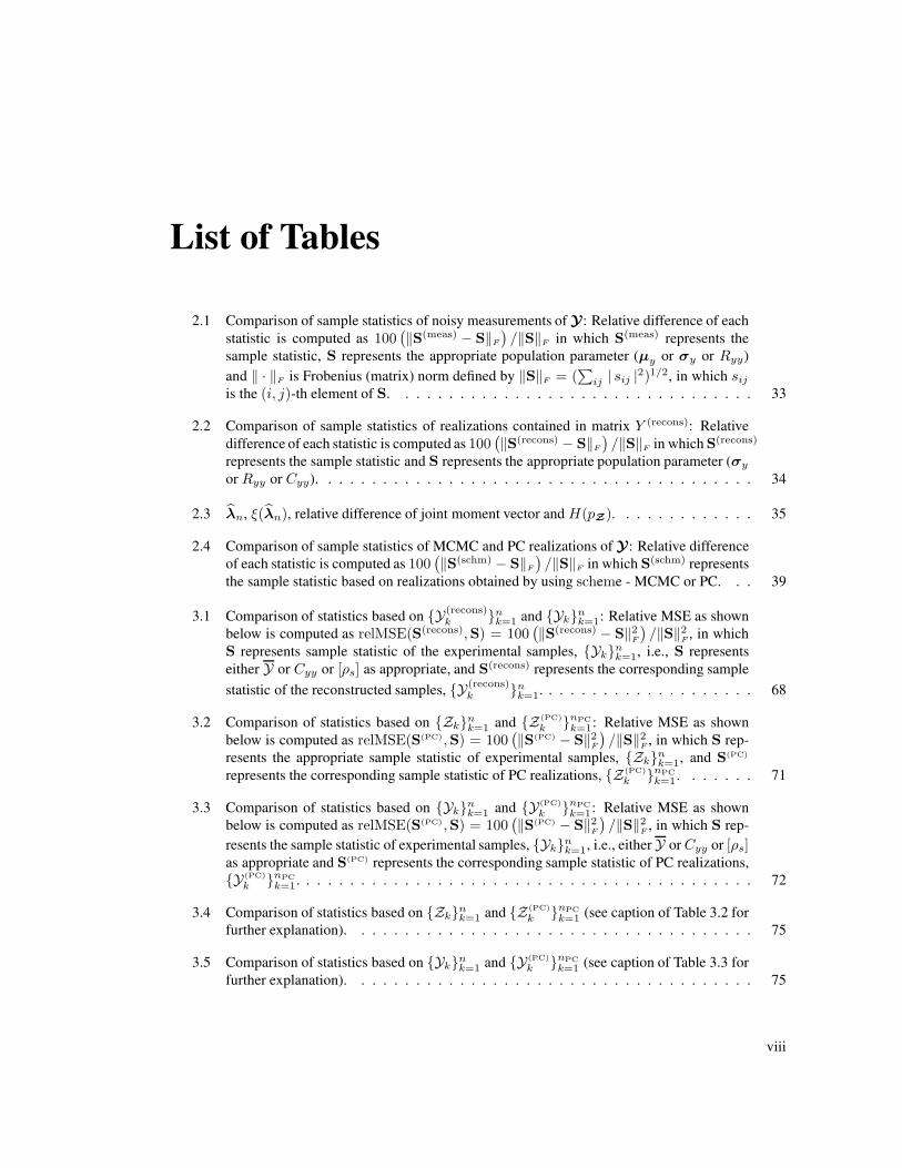
2.1 Comparison of sample statistics of noisy measurements of Y : Relative difference of each

statistic is computed as 100(‖S(meas) − S‖F

)/‖S‖F in which S(meas) represents the

sample statistic, S represents the appropriate population parameter (µy or σy or Ryy)

and ‖ · ‖F is Frobenius (matrix) norm defined by ‖S‖F = (∑

ij | sij |2)1/2, in which sij

is the (i, j)-th element of S. . . . . . . . . . . . . . . . . . . . . . . . . . . . . . . . . 33

2.2 Comparison of sample statistics of realizations contained in matrix Y (recons): Relative

difference of each statistic is computed as 100(‖S(recons) − S‖F

)/‖S‖F in which S(recons)

represents the sample statistic and S represents the appropriate population parameter (σy

or Ryy or Cyy). . . . . . . . . . . . . . . . . . . . . . . . . . . . . . . . . . . . . . . . 34

2.3 λn, ξ(λn), relative difference of joint moment vector and H(pZ). . . . . . . . . . . . . 35

2.4 Comparison of sample statistics of MCMC and PC realizations of Y : Relative difference

of each statistic is computed as 100(‖S(schm) − S‖F

)/‖S‖F in which S(schm) represents

the sample statistic based on realizations obtained by using scheme - MCMC or PC. . . 39

3.1 Comparison of statistics based on {Y(recons)k }n

k=1 and {Yk}nk=1: Relative MSE as shown

below is computed as relMSE(S(recons),S) = 100(‖S(recons) − S‖2

F

)/‖S‖2

F, in which

S represents sample statistic of the experimental samples, {Yk}nk=1, i.e., S represents

either Y or Cyy or [ρs] as appropriate, and S(recons) represents the corresponding sample

statistic of the reconstructed samples, {Y(recons)k }n

k=1. . . . . . . . . . . . . . . . . . . . 68

3.2 Comparison of statistics based on {Zk}nk=1 and {Z (PC)

k }nPC

k=1: Relative MSE as shown

below is computed as relMSE(S(PC),S) = 100(‖S(PC) − S‖2

F

)/‖S‖2

F , in which S rep-

resents the appropriate sample statistic of experimental samples, {Zk}nk=1, and S(PC)

represents the corresponding sample statistic of PC realizations, {Z (PC)

k }nPC

k=1. . . . . . . 71

3.3 Comparison of statistics based on {Yk}nk=1 and {Y(PC)

k }nPC

k=1: Relative MSE as shown

below is computed as relMSE(S(PC),S) = 100(‖S(PC) − S‖2

F

)/‖S‖2

F, in which S rep-

resents the sample statistic of experimental samples, {Yk}nk=1, i.e., either Y orCyy or [ρs]

as appropriate and S(PC) represents the corresponding sample statistic of PC realizations,

{Y(PC)

k }nPC

k=1. . . . . . . . . . . . . . . . . . . . . . . . . . . . . . . . . . . . . . . . . . 72

3.4 Comparison of statistics based on {Zk}nk=1 and {Z (PC)

k }nPC

k=1 (see caption of Table 3.2 for

further explanation). . . . . . . . . . . . . . . . . . . . . . . . . . . . . . . . . . . . . 75

3.5 Comparison of statistics based on {Yk}nk=1 and {Y(PC)

k }nPC

k=1 (see caption of Table 3.3 for

further explanation). . . . . . . . . . . . . . . . . . . . . . . . . . . . . . . . . . . . . 75

viii

List of Figures

2.1 Measurement locations of y(x,θ) over spatial domain D. . . . . . . . . . . . . . . . . . 30

2.2 Statistics of yq , q = 1, · · · , N . . . . . . . . . . . . . . . . . . . . . . . . . . . . . . . . 31

2.3 Euclidean norm, ‖β(MCMC)‖, of β(MCMC), representing the vector of sample joint-

moments estimated by using 2170 independent MCMC samples and shown as solid line,

is compared to ‖βn‖ shown as dashed line. . . . . . . . . . . . . . . . . . . . . . . . . 36

2.4 Fisher information matrix with known elements as marked; void part consists of unknown

elements. . . . . . . . . . . . . . . . . . . . . . . . . . . . . . . . . . . . . . . . . . . 37

2.5 Marginal probability density function of z3, pz3(z3). . . . . . . . . . . . . . . . . . . . 38

3.1 2-D Illustration: data points. . . . . . . . . . . . . . . . . . . . . . . . . . . . . . . . . 48

3.2 2-D Illustration: histogram. . . . . . . . . . . . . . . . . . . . . . . . . . . . . . . . . . 49

3.3 2-D Illustration: the target mjpdf, pY ≡ py1y2 , of Y = [y1,y2]T . . . . . . . . . . . . . 49

3.4 2-D Illustration: three slices representing the conditional pdf of y1, given y2 = y2, for

three different y2’s. . . . . . . . . . . . . . . . . . . . . . . . . . . . . . . . . . . . . . 50

3.5 2-D Illustration: three slices representing the conditional PDFs of y1, given y2 = y2, for

three different y2’s. . . . . . . . . . . . . . . . . . . . . . . . . . . . . . . . . . . . . . 50

3.6 2-D Illustration: j 7−→ aj(y2) for given y2. . . . . . . . . . . . . . . . . . . . . . . . . 52

3.7 2-D Illustration: y2 7−→ aj(y2) for given j ∈ N. . . . . . . . . . . . . . . . . . . . . . . 53

3.8 A few experimentally measured time histories (shown only for a segment of the total

experimental time span). . . . . . . . . . . . . . . . . . . . . . . . . . . . . . . . . . . 62

3.9 A typical quiescent zone divided into 9 smaller segments with 11 samples (shown for a

few sensors). . . . . . . . . . . . . . . . . . . . . . . . . . . . . . . . . . . . . . . . . 63

3.10 A typical subset of (T × D) with two time histories collected from tav309; dotted lines

indicate linear fit to the experimental data. . . . . . . . . . . . . . . . . . . . . . . . . . 64

3.11 A few typical profiles of experimental samples of Γ(n)(t, h); (t, h) 7−→ Γ(n)(t, h) at

h = 16 m depth. . . . . . . . . . . . . . . . . . . . . . . . . . . . . . . . . . . . . . . . 65

ix

3.12 Experimental variation of temperature measurements after removing the linear trends and

before normalization (shown for two time histories and over a quiescent zone). . . . . . 65

3.13 Variation of the normalized temperature measurements (shown for two time histories and

over a quiescent zone). . . . . . . . . . . . . . . . . . . . . . . . . . . . . . . . . . . . 66

3.14 Bivariate pdf of (zl, zu) corresponding to maxl∈L,u∈U [relMSEp(p(PC)zlzu

, pzlzu)] = 2.4136%

based on: (a) 216 experimental samples and (b) 50000 PC samples. . . . . . . . . . . . 71

3.15 Contour plots associated with the bivariate pdfs shown in Figure 3.14: (a) based 216experimental samples and (b) based on 50000 PC samples. . . . . . . . . . . . . . . . . 71

3.16 Marginal pdf of zi corresponding to maxi∈I [relMSEp(p(PC)zi

, pzi)] = 2.1833%. . . . . . 74

4.1 Mean built-up structure; E = 2.0 × 1011 N/m2, ρ = 7850 kg/m3, Circular section with

radius r = 0.025 m, Modal critical damping ξ = 0.001 over all modes; all dimensions

are in m. . . . . . . . . . . . . . . . . . . . . . . . . . . . . . . . . . . . . . . . . . . . 93

4.2 Dispersion parameters of receptance FRF matrices of nonparametric subsystems. . . . . 95

4.3 Statistical details of the deflection, W3,1, of the built-up structure (case 1). . . . . . . . . 96

4.4 Statistical details of the deflection, W3,1, of the built-up structure (case 2). . . . . . . . . 97

4.5 Normal probability plot of |W3,1| at ω = 42 Hz (case 1). . . . . . . . . . . . . . . . . . 98

4.6 Normal probability plot of |W3,1| at ω = 42 Hz (case 2). . . . . . . . . . . . . . . . . . 98

4.7 Normal probability plot of ln (|W3,1|) at ω = 208 Hz (case 1). . . . . . . . . . . . . . . 99

4.8 Normal probability plot of ln (|W3,1|) at ω = 208 Hz (case 2). . . . . . . . . . . . . . . 99

5.1 Heterogeneity of Al2024 at two different scales (mesoscopic regime). . . . . . . . . . . 104

5.2 Typical test samples of unit area; the black phase represents inclusion and the spatial

regions of the inclusions are randomly selected; FE analysis done with 9-node quadrilat-

eral plane stress elements. . . . . . . . . . . . . . . . . . . . . . . . . . . . . . . . . . . 131

5.3 A 2D homogenized cantilever beam modeled with 9-node quadrilateral nonparametric

plane elements; the total load P is distributed parabolically as shown with a dashed line

at x = L. . . . . . . . . . . . . . . . . . . . . . . . . . . . . . . . . . . . . . . . . . . 136

5.4 Estimate of the pdf of tr(Ceff) and of the volume averaged strain energy, ϕ, based on Ns

samples. . . . . . . . . . . . . . . . . . . . . . . . . . . . . . . . . . . . . . . . . . . . 137

5.5 Statistics of the random response of the cantilever beam; Uy(x) represents the random

displacement of the beam in y-direction along the center line of the beam, y = 0;

E[Uy(x)] is the sample mean of Uy(x) estimated based on Ns samples. . . . . . . . . . 138

x

Abstract

This dissertation focusses on characterization, identification and analysis of stochastic systems. A stochas-

tic system refers to a physical phenomenon with inherent uncertainty in it, and is typically character-

ized by a governing conservation law or partial differential equation (PDE) with some of its parameters

interpreted as random processes, or/and a model-free random matrix operator. In this work, three data-

driven approaches are first introduced to characterize and construct consistent probability models of non-

stationary and non-Gaussian random processes or fields within the polynomial chaos (PC) formalism.

The resulting PC representations would be useful to probabilistically characterize the system input-output

relationship for a variety of applications. Second, a novel hybrid physics- and data-based approach is

proposed to characterize a complex stochastic systems by using random matrix theory. An application of

this approach to multiscale mechanics problems is also presented. In this context, a new homogenization

scheme, referred here as nonparametric homogenization, is introduced. Also discussed in this work is a

simple, computationally efficient and experiment-friendly coupling scheme based on frequency response

function. This coupling scheme would be useful for analysis of a complex stochastic system consisting of

several subsystems characterized by, e.g., stochastic PDEs or/and model-free random matrix operators.

While chapter 1 sets up the stage for the work presented in this dissertation, further highlight of each

chapter is included at the outset of the respective chapter.

xi

Chapter 1

Introduction

Quantifying confidence in model-based predictions is an essential step towards model validation, requir-

ing an analysis of uncertainty in the representation of physical phenomena, in data acquisition and rep-

resentation, and in the numerical resolution of the resulting, possibly stochastic, governing equations.

Casting this validation problem in a probabilistic context requires the probabilistic characterization of

system parameters from experimental evidence, and the propagation of the associated uncertainty to the

predictions of the corresponding mathematical model.

Two venues have generally been pursued for the probabilistic representation of system parameters,

associated with parametric and nonparametric models. Parametric models typically refer to the govern-

ing conservation law or partial differential equation, interpreting some of the associated parameters as

intrinsically random [MI99, GS91, KTH92] thereby modeling them as random processes or/and fields.

The statistical characterization of these models is a well developed topic with a significant set of tools to

draw from. Typical statistics derived from these representations include marginal and multi-point statistics

(usually two and three-point statistics) [CBS00, Chapter 3], including correlation functions and spectral

density functions. A physical phenomenon modeled as a stochastic system with a lower level of uncer-

tainties or/and with a relatively fewer number of random system parameters is well suited for analysis

within the parametric formalism.

Nonparametric models, on the other hand, refer to the predictive model as a random operator usually

resulting in random matrix perturbations to some nominal deterministic matrix equation [Soi00, Soi01a].

While the initial development of nonparametric models has evolved around particular physical models in

which specific probability distributions of matrix-valued random variables have been analytically derived

[Meh04, TV04], their recent application to broader problems in science and technology has required novel

adaptation of statistical estimation and identification methods [Soi99, Soi00, Soi01a, Soi05a, Soi05b].

Since it refers to the class of models in which the available information needs to be expressed only

through a set of system matrices/tensors (for example, mass matrix, stiffness matrix, damping matrix or

1

elasticity tensor), a system having a higher level of uncertainties or/and a system with a large number

of random local system parameters (for example, fluid permeability, Young’s modulus, shear modulus,

bulk modulus, Poisson’s ratio etc.) is more amenable to the nonparametric approach. It does not require

any information at the local system parameter level as needed in a parametric formulation. At the current

stage, most of these methods are, however, still limited to assimilating first order statistics of experimental

observations along with a certain (scalar-valued) second-order statistic. This promising technique has

recently been applied in a number of practical applications [CLPP+07, ACB08].

The work presented in this dissertation considers both the models in characterizing the uncertainty of

stochastic systems. Works in chapter 2 and chapter 3 are carried out within the parametric framework.

A simple coupling technique to combine nonparametric system and parametric system is described in

chapter 4. Finally, the work presented in chapter 5 considers the nonparametric model in more detail

and propels the existing nonparametric techniques a little bit forward. While motivation behind the work

presented in each chapter is reflected in the corresponding chapter, a glimpse of the overall works is in

order before proceeding further.

1.1 Outline

The topics of chapter 2 and chapter 3, within the parametric framework, primarily deal with the character-

ization of a non-stationary and non-Gaussian random process or field by using a set of measurement data.

While the conventional probabilistic characteristics, e.g., probability density functions, correlation func-

tion etc., are informative in a descriptive context, they cannot be efficiently propagated through predictive

physics-based models. This is largely due to the difficulty associated with synthesizing realizations of

non-Gaussian and non-stationary random vectors and stochastic processes from the knowledge of their

statistical moments.

In recent years, the polynomial chaos (PC) expansion [GS91] has been used to a great advantage

in representing tensor-valued stochastic processes and characterizing solutions to the associated stochas-

tic governing differential equations. Within the purview of the PC framework, the probability model of

the random process refers to a spectral decomposition constructed with respect to (w.r.t.) a set of basis

functions in a suitable linear space. The basis functions constitute a set of orthogonal functions w.r.t. a

2

properly chosen probability measure [GS91, XK02, SG04a]. The coordinates (often referred as PC coeffi-

cients in the literature) w.r.t. the basis functions are the representative statistics. The set of PC coefficients

play the similar role within the PC framework as played by the parameters of a characterizing multivari-

ate joint probability density function (mjpdf) (for example, the mean vector and the covariance matrix of

a multidimensional Gaussian distribution) within the conventional probability framework. Representing

the random process by using PC expansion has some added advantages over the conventional probabil-

ity framework. It facilitates in performing rigorous convergence analysis of the error in representing the

system parameters (modeled as a random process) and its effect on the model-based predictions by using

the machinery already available in the field of functional analysis. Furthermore, the PC representation

presents a mechanism for easy simulation of the random process thus making it a viable alternative even

within the conventional ensemble-based probability framework.

The PC formalisms thus provides a theoretically sound backbone facilitating efficient construction of

the probability model of the non-stationary and non-Gaussian second-order random process possibly rep-

resenting some model parameters of a stochastic system [Gha99, XK02, DNP+04, LMNGK04, SG04a].

It has been proven to be a useful tool for systematic propagation of the statistical properties of these

stochastic system parameters to the response of the model in a diverse field of applications [GS91, Gha99,

GRH99, PG00, XLSK02, RNGK03, DNM+03, SG04a, GGRH05, GSD07, LMNP+07, WSB07]. The

works presented in chapter 2 and chapter 3, therefore, focus on constructing the PC representation of a

random process from data.

Chapter 4 and chapter 5 investigate the issues of nonparametric models. A coupling technique, that

can couple several systems each of which, in its uncoupled state, is most suitable to either parametric or

nonparametric modeling, is presented in chapter 4. A new probabilistic formulation within the nonpara-

metric framework is proposed in chapter 5 to characterize a positive-definite random system matrix that

is bounded from below and above in positive-definite sense.

1.2 Notation and Terminology

Throughout this work, bold face character would be used to indicate that the quantity under consideration

is either random or multidimensional. The realizations of a multidimensional random quantity are, how-

ever, denoted by the respective normal characters for distinction purpose. Though every attempt would be

3

made to follow this convention, there might be violations at a few places but only if there exist no room

for ambiguity.

Since a part of the current work considers the problem of constructing the probability model of a

non-stationary and non-Gaussian random process, a clarification of terminology for the present work is

set forth now. When the indexing set of the stochastic process is multidimensional, reference is often

made to a random field, and a stationary random process is then referred to as a homogeneous random

field. In this work, and to emphasize the identical underlying mathematical structure, the term ‘stochastic

process’ or ‘random process’ would be ubiquitously used and the equivalent concepts of homogeneity

and stationarity would be implied by default.

In the context of works presented in chapters 2–3, the term ‘probability model’ refers to ‘PC repre-

sentation’.

The term ‘random variate’ or ‘random variable’ would be succinctly used throughout this work to

indicate scalar-, vector-, matrix- or tensor-valued random variable, which would be clear from the con-

text.

4

Chapter 2

Asymptotic Distribution for PC

Representation from Data

A procedure is presented in this chapter for characterizing the asymptotic sampling distribution of estima-

tors of the PC coefficients of a second-order non-stationary and non-Gaussian random process by using a

collection of observations. The random process represents a physical quantity of interest, and the obser-

vations made over a finite denumerable subset of the indexing set of the random process are considered

to form a set of realizations of a random vector, Y , representing a finite-dimensional projection of the

random process. The Karhunen-Loeve (KL) decomposition and a scaling transformation are employed

to produce a reduced order model, Z, of Y . The PC expansion of Z is next determined by having

recourse to the maximum-entropy (MaxEnt) principle, Metropolis-Hastings (M-H) Markov chain Monte

Carlo (MCMC) algorithm and the Rosenblatt transformation. The resulting PC expansion has random

coefficients; where the random characteristics of the PC coefficients can be attributed to the limited data

available from the experiment. The estimators of the PC coefficients of Y obtained from that of Z are

found to be maximum likelihood estimators (MLE) as well as consistent and asymptotically efficient.

Computation of the covariance matrix of the associated asymptotic normal distribution of estimators of

the PC coefficients of Y requires knowledge of the Fisher information matrix (FIM). The FIM is evaluated

here by using a numerical integration scheme as well as a sampling technique. The resulting confidence

interval on the PC coefficient estimators essentially reflects the effect of incomplete information (due to

data limitation) on PC representation of the stochastic process. This asymptotic distribution is signifi-

cant as its characteristics can be propagated through predictive model for which the stochastic process in

question describes uncertainty on some input parameters.

5

2.1 Motivation and Problem Description

Many applications in science and engineering involve modeling spatio-temporal phenomena. Within the

confines of the probabilistic framework, the Gaussian stochastic process has been the most commonly

used form for modeling such physical phenomena. In addition to the constraint provided by the form of

the probability measure when using such a process, additional simplifying assumptions such as station-

arity, separability and symmetry are usually made in constructing it for mathematical convenience and

computational expediency. The construction of Gaussian processes from finite data continues to be an

active field of research with issues such as multidimensionality, non-symmetry, and non-stationarity pro-

viding the motivation for much of the innovation [GGG05]. The development of non-Gaussian models,

on the other hand, has been much slower; certainly to a slower extent than the Gaussian models, chiefly

due to the scarcity of consistent mathematical theories for describing infinite-dimensional probability

measures.

In addition to the mathematical challenges introduced by the quest for non-Gaussian stochastic mod-

els, a very important difficulty is presented by the scarcity of data on which these models are to be based.

Since Gaussian processes are characterized only by their mean and covariance functions, they require

a manageable amount of information and thus often provide a rational modeling alternative. This has

limited the scope of non-Gaussian models to transformations of Gaussian vectors and processes, or to

models that are completely characterized by their lower order statistics. These challenges notwithstand-

ing, it remains a recognized fact that many processes representing physical phenomena rarely satisfy the

assumptions and constraints associated with a Gaussian process. (See section 3.1 for a more exhaustive

discussion on the currently existing procedures to characterize non-Gaussian random processes).

As highlighted in chapter 1, a significant benefit of the PC formalism lies in its ability to characterize

non-Gaussian, non-stationary and multidimensional second-order stochastic processes and the potential

for its efficient implementation into predictive models. Therefore, the work in this chapter focuses on

the construction and characterization of PC representation of a non-stationary and non-Gaussian random

process only from data.

It is assumed in the present work that the stochastic process under consideration is a second-order ran-

dom process. This assumption guarantees the existence of its PC representation. From the vantage point

of the fact that the most physically measurable random processes are second-order type, this assumption

6

is not a severe restriction. The PC expansion of a second-order (scalar-, vector-, matrix or tensor-valued)

stochastic process is a spectral decomposition in terms of a set of orthogonal basis functions constructed

w.r.t. a suitable and known probability measure of user’s choice. Typical PC decompositions have been

developed w.r.t. basis functions representing Hermite polynomials in Gaussian variables [GS91], poly-

nomials that are orthogonal w.r.t. a variety of measures [XK02] and multi-wavelet basis [LMNGK04].

Convergence results for PC representations are well-established for functionals of Gaussian processes

[CM47] and for functions of finite-dimensional random vectors with arbitrary measure [XK02, SG04a].

As indicated earlier, the particular statistics characterizing the PC representation consist of PC coef-

ficients or coordinates of the process w.r.t. the chosen set of orthogonal basis functions. The algebraic

character of the PC coefficients (scalars, vectors, functions or vector-, matrix- or tensor-valued functions)

is inherited from the stochastic quantity they represent. Using these linear decompositions of stochastic

vectors and processes, the mapping of probabilistic measure from stochastic system parameters to system

state follows from a mapping between the PC coefficients of the system and state processes. This lat-

ter mapping is a deterministic transformation, obtained from the original stochastic governing equations

through algebraic manipulations and projections in suitable linear spaces [GS91, Gha99, GRH99].

Consider a physical phenomenon defined over D ⊂ Rd with Rd representing the Euclidean d-space,

and D typically referring to a spatio-temporal domain. Assume that this physical process is modeled

as a stochastic process, y(x,θ), on D × Θ with probability space (Θ,FΘ, µ). Consider a sequence

of possible observations of y(x,θ) at N locations over D with coordinates x1,x2, · · · , xN . Denote

the random variables associated with the random process, y(x,θ), at these locations by yq ≡ y(xq ,θ),

q = 1, 2, · · · , N , and let Y = [y1,y2, · · · , yN ]T where T represents the transpose operator. It should be

clear that Y represents a finite-dimensional representation of the original (infinite-dimensional) stochastic

process. Denote the multivariate joint probability distribution function (mjPDF; contrast it with mjpdf

abbreviated earlier for multivariate joint probability density — not distribution — function) of Y by

Py1,··· ,yN . The probability measure of the underlying random process is then completely characterized

by the family of mjPDF: {Py1,··· ,yN}, ∀N ≥ 1. Since N is always finite in an experimental or numerical

context, characterizing the underlying stochastic process has to be performed, in some approximate sense,

through Y . The value of N , required to achieve a certain fidelity in the finite-dimensional representation,

depends on the characteristics of the stochastic fluctuations of the original stochastic process over its

spatio-temporal domain (think of, e.g., correlation length).

7

In many practical situations, each component of Y can often be sufficiently well characterized by a

finite-dimensional PC representation. In these cases, a first level approximation is thus introduced while

selecting the dimension, nd < ∞, of the PC representation. For a component of Y associated with a

specified x, consider the leading P terms in this nd-dimensional (D) PC representation of y(x,θ) and,

let hx be the P -D vector consisting of these PC coefficients. In most physical applications, it cannot be

verified in general if such hx exists or not, and even if it exists, it cannot be specified exactly. It is assumed

in this work that such an unknown hx exists. Further, let hx denote the P -D vector representing an

estimator of hx based on available information. The elements of hx are computed based on a finite set of

noisy measurements that are typically observed on Y . Let, furthermore, hx be the P -D vector consisting

of the PC coefficients of the appropriate random variable component of Y satisfying limN→∞ hx = hx.

While the error ‖hx − hx‖ (‖ · ‖ represents a suitable norm, say, the Euclidean vector norm in RP )

can be reduced by increasing N , the error ‖hx − hx‖, conditioned on hx, can be monitored and reduced

by increasing the statistical significance of the sample from which the PC coefficients of Y are estimated.

The total error, ‖hx − hx‖, is bounded by,

‖hx − hx‖ ≤ ‖hx − hx‖ + ‖hx − hx‖ a.s., (2.1)

in which a.s. indicates that the above inequality is valid in almost sure (a.s.) sense w.r.t. the probability

measure, µ. It is assumed here that the second error term, ‖hx − hx‖, is known either deterministically

(for example, in the sense that the effect of finite N would be negligible if N is large enough so that Y

encompasses all the statistical characteristics of interests of y(x,θ) with sufficient accuracy) or statisti-

cally. The work presented in this chapter, on the other hand, focuses on the first error term ‖hx − hx‖,

conditioned on hx, that can be sharpened through data acquisition.

Recent work in this direction has relied on the maximum likelihood principle to estimate the PC coef-

ficients based on an approximate mjpdf of the dominant KL random variable components of the stochastic

process [DGS06, DSG07] that simplifies the form of the likelihood function for computational expedi-

ency (this computational scheme bears some resemblance to the composite likelihood method [Lin88]).

Additional related work has assumed the KL components to be statistically independent and estimated

their probability density functions using either Bayesian inference [GD06] or a histogram constructed

from observations of the KL variables [BLT03]. It should be noted that a number of previous efforts

8

[BLT03], while constructing the probability density function (pdf) estimates of the KL variables, did not

provide a method for constructing or using associated sampling distributions which could otherwise have

been used as indicators to the sensitivity of the probabilistic model to additional observations.

As already explained, the work here focuses primarily on the error, due to the inexact representation

of the stochastic process because of data limitations, for a general class of problems. A framework and

its numerical implementation for the statistical analysis of this error, that would be useful to determine its

impact on model-based prediction, is presented. Use of the PC representation of the stochastic process

expressed with sufficient accuracy in terms of the statistically dependent dominant KL random variables

makes the procedure very efficient in propagating the error to the model-based predictions. In particular,

an asymptotic distribution, conditioned on hx, is identified for hx − hx, and a computational scheme for

its evaluation is presented. Given the Gaussian form of this distribution (see section 2.2.4), the propagation

of this error through the system prediction can be readily formulated, thus enabling the assessment of the

sensitivity of model-based predictions to refinement in the statistics of the model parameters.

Though the primary goal of the current chapter is to present a framework for analyzing the signifi-

cance of data error in the background of PC formalisms, several tools, from the fields of MaxEnt principle

and FIM, are also needed for successful completion of the work here. The MaxEnt principle is employed

to estimate the mjpdf of a random vector, representing a reduced order model of Y , consisting of M

dominant and statistically dependent KL random variables. It must be remarked here that though the

MaxEnt principle is known for several decades, it is primarily and successfully used for the estimation of

pdfs of scalar random variables and for a limited class of multivariate problems. Moreover, in the existing

statistical literature, it is hard to find any appealing, reliable and computationally efficient density estima-

tion technique for a set of statistically dependent random variables from a set of finite samples. A brief

introduction of the principle of maximum entropy, its appealing features and a computational scheme for

density estimation in the context of the present work are provided in section 2.3.1. The FIM, on the other

hand, is required to compute the covariance matrix of the asymptotic normal distribution. This matrix is

an indicator of the amount of information contained in the observed data about quantities of interest typi-

cally representing some model parameters. Prominent areas of applications of the FIM include, to name

a few, confidence interval computation of model parameters [CLR96, HD97], determination of inputs

to nonlinear models in experimental design [Spa03, Section 17.4] and determination of noninformative

prior distribution (Jeffreys’ prior) for Bayesian analysis [Jef46]. The FIM, in the present context, would

9

be useful to compute the confidence interval of the error term, ‖hx − hx‖, conditioned on hx. A brief

discussion on this matrix in light of the present work and the required estimation technique is presented

in section 2.3.4.

The chapter begins with the development of a reduced order model for Y by using its KL decompo-

sition. The resulting M -D (with M < N ) random vector associated with the dominant subspace will be

referred as the KL vector which is subsequently transformed to another M -D random vector supported

on an M -dimensional hypercube, [0 1]M . This new random vector will be referred as the normalized

KL (nKL) vector. An estimation of the mjpdf of the nKL vector is then obtained by using the MaxEnt

technique. Following that, a Markov chain is constructed and used to estimate the PC representation

of the nKL vector from which estimators of the PC coefficients of Y are determined. The asymptotic

probability density function (apdf) of estimators of the PC coefficients of Y is then identified in order to

statistically characterize the first error term in (2.1). The procedure is demonstrated by an example and

the final section contains the conclusion inferred from the work presented in this chapter.

The proposed use of the Rosenblatt transformation in constructing the PC representation of a random

vector in section 2.2.3 and identification of the asymptotic distribution in section 2.2.4 are the origi-

nal contributions of the present chapter to the literature of computational statistics. The computational

scheme, as described in section 2.3.3, is also a noteworthy addition to the set of computational statistics

tool for mjpdf estimation by matching a target set of higher order joint statistics of a random vector.

2.2 Representation and Characterization of the Random Process

from Measurements

The KL expansion [Loe78, Chapter XI], [Jol02] is first employed to optimally reduce the number of

random variables needed to characterize Y yielding, in the process, a set of uncorrelated random variables.

Then, the PC coefficients of y(x,θ) are determined via estimating the PC coefficients of the reduced order

model.

10

2.2.1 Karhunen-Loeve Decomposition: Reduced Order Representation of the

Random Process

Suppose that n observations of Y , denoted by Y1, · · · ,Yn, have been collected. An unbiased estimate of

the mean vector of Y is given by Y = (1/n)∑n

k=1 Yk , and an estimate of the N ×N covariance matrix

byCyy = (1/(n−1))YoYTo in which Yo = [Y1o, · · · ,Yno] represents anN×nmatrix and Yko ≡ Yk−Y ,

k = 1, · · · , n. Let the i-th, i = 1, · · · , N , largest eigenvalue of Cyy be denoted by ςi and the associated

eigenvector by Vi. Following the KL expansion procedure, let us now collect the dominant KL random

variable components, {z′1, · · · , z′M}, M < N , in an M -D random vector, Z′ = [z′1, · · · , z′M ]T . The

M random variables, z′i, i = 1, · · · ,M , are zero-mean and uncorrelated (but not necessarily statistically

independent), and have unbiased estimates of variances given by ςi’s. The value of M is chosen such that

tr(Cyy) =∑N

i=1 var(yi) ≈∑M

i=1 ςi =∑M

i=1 var(z′i) with var and tr, respectively, representing variance

and trace operators. Here, Z′ is related to Y by,

Z′ = V T (Y − Y), (2.2)

in which V = [V1, · · · , VM ] is the N ×M matrix of eigenvectors, V1, · · · , VM . The random vector, Z′,

will be referred now on as the KL vector.

The set of experimental samples of Z′ can be immediately obtained by replacing Y with Y1, · · · ,Yn

in (2.2) resulting in Z ′1, · · · ,Z ′

n. To enhance the regularity of the ensuing numerical problem and improve

the efficiency of the associated computation, the following scaling is applied to the data on Z′ obtaining

a set of realizations of a new random vector,

Zk =

[(Z ′

k − a)◦(

1

b− a

)], k = 1, · · · , n. (2.3)

Here, the symbol ◦ represents element-wise product operator or the Hadamard product operator, a =

[a1, · · · , aM ]T and b = [b1, · · · , bM ]T with ai = min(z′(1)i , · · · , z′(n)

i ) and bi = max(z′(1)i , · · · , z′(n)

i ), in

which z′(k)i is the i-th component of the k-th sample, Z ′

k = [z′(k)1 , · · · , z′(k)

M ], and finally, 1/(b− a) needs

to be interpreted as M × 1 column vector with its i-th, i = 1, · · · ,M , element being given by reciprocal

of the i-th element of (b − a). Denote the resulting M -D random vector associated with the samples,

{Zk}nk=1, by Z = [z1, · · · , zM ]T supported onM -dimensional unit hypercube, Ξ ≡ [0 1]M ⊂ RM . The

11

random vector, Z, having uncorrelated and non-zero mean components, will be referred as the normalized

KL (nKL) vector. The following relation between Z and Y then holds,

Y ≈ Y(M) = [V (b+ a◦Z)] + Y. (2.4)

The approximation sign, ‘≈’, in (2.4) is indicated due to the fact that Y is projected into the space spanned

only by the largest M dominant eigenvectors of Cyy to obtain the reduced order representation, Z . Next,

a sampling-based technique for computing an estimate of the vector, hx, of the PC coefficients of y(x,θ)

is described via estimating the PC coefficients of Z . A description of the PC formalism is, however, first

reviewed before estimating the PC coefficients of Z from {Zk}nk=1.

2.2.2 Polynomial Chaos Formalism

The current state-of-the-art PC approach is the evolution of the repertoire of Cameron and Martin [CM47],

where a second-order non-linear function(al), defined on the space, C, of all real-valued continuous func-

tions on a compact support, is approximated by a spectral decomposition constructed w.r.t. a set of

multidimensional orthogonal Hermite polynomials. The set of Hermite polynomials is constructed w.r.t.

a set of statistically independent Gaussian random variables. They particularly investigated the issue of

convergence as the dimension (representing the number of Gaussian random variables) tends to infinity. It

is shown [CM47] that the resulting spectral representation converges to the non-linear function(al) being

approximated in mean-square sense as the dimension and order of the multidimensional Hermite polyno-

mials tend to infinity. The mean-square error (MSE) is measured w.r.t. the Wiener measure [Wie38], on

C. The Wiener measure is used to represent the integral of a Brownian motion associated with (infinite-

dimensional) Gaussian white noise process.

The aforesaid work involving infinite-dimensional Gaussian measures has been adapted to the finite-

dimensional Gaussian and non-Gaussian measures by employing several novel schemes. Accordingly,

the PC representation of second-order random process and random vector have been developed in terms

of orthogonal polynomials constructed w.r.t. a set of statistically independent Gaussian random vari-

ables [GS91, Gha99, GRH99, DNP+04] as well as non-Gaussian random variables [XK02]. The doubly

orthogonal polynomials, assuming that the KL random variable components of the stochastic process are

12

statistically independent [BTZ05], and the wavelet basis functions, constructed w.r.t. statistically inde-

pendent non-Gaussian random variables [LMNGK04] (also see [PB06] for a related application), have

recently been implemented as basis functions in the construction of PC representation. The theoretical

development of employing orthogonal polynomials, that are constructed w.r.t. a set of statistically depen-

dent second-order random variables, has also been accomplished [SG04a].

Denote the number of random variables to be included in the PC representation (i.e., dimension of the

PC representation) by nd. While increasing the dimension of the PC expansion provides added freedom

in the representation, it significantly increases the computational cost. A balance must be thus reached

among flexibility of the representation, available computational resources and target accuracy. Let ξ ≡

(ξ1, · · · , ξnd) be a Rnd-valued random vector defined on (Θ,FΘ, µ) with its induced mjPDF being

denoted by Pξ. The probability measure, Pξ, is chosen such that it is best amenable [XK02, SG04a,

LMNGK04] to the PC representation of zk ≡ zk(ξ) thus adapting its choice to the known probabilistic

characteristics of zk(ξ). It is also assumed that Pξ admits a joint pdf, pξ, verifying dPξ(ξ) = pξ(ξ) dξ,

with dξ being given by dξ =∏nd

i=1 dξi in which dξi is the Lebesgue measure on R. Based on chosen Pξ,

the PC representation of each component of Z can be expressed as,

zk ≡ zk(ξ) =∑

α∈Nnd

zα,k Υα(ξ), k = 1, · · · ,M, (2.5)

if zk(ξ) is second-order random variable, i.e., E[|zk(ξ) |2] <∞ with |x | representing the absolute value

of x andE[ · ] representing the expectation operator w.r.t. the chosen probability measure, Pξ (this second-

order condition is satisfied here since the underlying stochastic process is assumed to be second-order).

Here, N = {0, 1, 2, · · · }, {zα,k,α ≡ (α1, · · · , αnd) ∈ Nnd} is the set of PC coefficients representing the

coordinates w.r.t. the set of basis functions, {Υα,α ∈ Nnd}, given by [SG04a],

Υ0(ξ) = 1, if α = 0 ∈ Nnd ,

Υα(ξ) =

(∏nd

i=1 pξi(ξi)

pξ(ξ)

)1/2 nd∏

i=1

Ψαi(ξi), if α 6= 0.(2.6)

Here, pξiis the marginal pdf (marpdf) of ξi induced by pξ and Ψαi(ξi) are polynomials of order αi in ξi.

These polynomials are orthogonal to each other in the sense thatE[Ψj(ξi)Ψl(ξi)] = 0 for j 6= l, in which

E[ · ] is the expectation operator w.r.t. the probability measure, Pξi, that admits dPξi

(ξi) = pξi(ξi) dξi.

13

As already indicated, this also implies [SG04a] the orthogonality of the set, {Υα(ξ),α ∈ Nnd}, w.r.t.

Pξ. In the case of statistically independent random variables, (2.6)2 simplifies to,

Υα(ξ) =

nd∏

i=1

Ψαi(ξi). (2.7)

The equality, ‘=’, in (2.5) should be interpreted in the mean-square sense such that E[{yk(ξ) −∑

α:|α|≤noyα,k Υα(ξ)}2] −→ 0 as no −→ ∞, where the expectation operator is w.r.t. Pξ [SG04a],

|α |= ∑nd

i=1 αi, and no is the maximum order (i.e., order of the PC representation) of all the basic

orthogonal polynomials, {Ψαi , αi ∈ N, i ∈ (1, · · · , nd)}, included in (2.5). Given nd and chosen no,

the number of basis functions retained in the infinite series of (2.5) is given by (including the 0-th order

basis function), (P + 1) = (no + nd)!/(no! nd!) that clearly tends to infinity as n0 −→ ∞. This implies

that the accuracy (in the sense of mean-square error (MSE) reduction) of the PC representation can be

improved by only increasing the order, n0. However, for computational purpose, this infinite series is

truncated after a finite number of terms that is typically determined by the available computational budget

and target accuracy (usually in terms of MSE).

The flexibility and the accuracy of the PC representation also depend on the choice of Pξ and con-

sequently, on the resulting set of orthogonal basis functions used in (2.5). The proper selection of the

probability measure, Pξ, may be dictated by the physical or experimental or modeling features involved

in treating the physical process of interest as stochastic process. This stochastic process is, therefore,

viewed as a (possibly nonlinear) transformation of ξ1, · · · , ξndrepresenting those features. However,

different choice of suitable Pξ is also theoretically plausible, and might be preferred for a relatively less

computational expense required to achieve an equivalent or more statistically significant representation

(in some appropriate sense, for example, in the sense of minimum MSE). Once the choice for Pξ is made

and the mapping, ξ 7−→ zk(ξ), is identified (either explicitly or implicitly), the PC coefficients can be

computed by using the orthogonality property of Υα’s,

zα,k =E[zk(ξ)Υα(ξ)

]

E[Υ2

α(ξ)] , α ∈ N

nd and k = 1, · · · ,M. (2.8)

14

The denominator in (2.8) can be evaluated by using (2.6) or (2.7) as appropriate. When ξ1, · · · , ξndare

statistically independent, then E[Υ2

α(ξ)]

reduces to, the denominator in (2.8) reduces to,

E[Υ2

α(ξ)]

=

nd∏

i=1

E[Ψ2

αi(ξi)

], (2.9)

in which E[Ψ2

αi(ξi)

]can often be extracted from the existing literature [Leb72, Chapter 4], [GS91,

XK02, SG04a] for many commonly employed measures, Pξi’s.

The numerator in (2.8), on the other hand, is given by,

E[zk(ξ)Υα(ξ)

]=

∫

Sξ

zk(ξ)Υα(ξ) pξ(ξ) dξ, (2.10)

in which Sξ ⊆ Rnd is the support of ξ. In the discussion until now, the existence of the mapping,

ξ 7−→ zk(ξ), is implicitly implied. Recent developments in PC representations have predominantly

treated problems where such a mapping is defined, either implicitly or explicitly. In the current work,

however, this mapping is unknown since the information, that is assumed to be available, is only the

measurement data on Y (i.e., in turn, on Z). A sampling based-technique for evaluating the numerator in

(2.8) is next described.

2.2.3 Polynomial Chaos Representation from Data

In general the random variables, {ξi}ndi=1, could be statistically dependent. The case of statistically inde-

pendent components is, however, of particular interest because of the additional computational efficiency

involved in evaluation of the integral in (2.10). After all the probability measure, Pξ, is a suitable choice

of the analyst! (It would be more clear later in chapter 3). For statistically independent {ξi}nd

i=1, the

integral in (2.10) reduces to,

E[zk(ξ)Υα(ξ)

](2.11)

=

∫

Sξ1

· · ·∫

Sξnd

zk(ξ)

(nd∏

i=1

Ψαi(ξi)

)pξ1

(ξ1) · · · pξnd(ξnd

) dξ1 · · ·dξnd,

in which Sξi⊆ R is support of ξi.

15

To establish the required mapping, ξ 7−→ zk(ξ), an inverse approach is adopted now, which would

facilitate in carrying out the integral in (2.11). The Rosenblatt transformation [Ros52] is used to relate

the nd-variate PDF, Pξ, associated with (2.11), and an absolutely continuous M -variate PDF, PZ , of Z.

This step imposes the condition that nd = M . The mapping defined by the Rosenblatt transformation

(as described next) is continuous. A requirement for using the Rosenblatt transformation is absolute

continuity of PZ .

Note that PZ represents an estimate of the PDF of Z obtained by using a suitable density estimation

technique. It is assumed for the time being that an estimate of the PDF of Z is available1. Suppose thatPZ

is characterized by p parameters, λ1, · · · , λp, represented as a p × 1 column vector, λ = [λ1, · · · , λp]T .

For example, the free elements characterizing a multivariate normal distribution function i.e., elements

of the mean vector, µ, and elements on and above the diagonal of the covariance matrix, Σ, might

constitute the column vector λ or, for a second example, the mean vector µ and the covariance matrix Σ

could as well depend on λ by some known deterministic (functionally implicit or explicit) relationships,

µ = µ(λ) and Σ = Σ(λ). This parameter vector, λ, needs to be estimated by using a suitable density

estimation technique and depends on the measurement data, and essentially characterizes the random

process, y(x,θ), through its reduced order representation, Z .

Consider the Rosenblatt transformation, T : Z 7−→ ξ, defined by,

Pξ1(ξ1)

d= P1(z1),

Pξ2(ξ2)

d= P2|1(z2),...

PξM(ξM )

d= PM|1:(M−1)(zM ),

⇒

ξ1d= P−1

ξ1(P1(z1)) ,

ξ2d= P−1

ξ2

(P2|1(z2)

),

...

ξMd= P−1

ξM

(PM|1:(M−1)(zM )

),

(2.12)

in which Pi|1:(i−1), i = 1, · · · ,M , is the PDF of zi conditioned on z1 = z1, z2 = z2, · · · , zi−1 = zi−1

induced by PZ . The equalities, “d=”, above should be interpreted in the sense of distribution implying

that the PDFs of the random variables in the left-hand-side (lhs) and the right-hand-side (rhs) of each

equality are identical [HLD04, Theorem 2.1]. For instance, consider Pi|1:(i−1)(zi) and Pξi(ξi) that are

two random variables (functions of zi and ξi, respectively), and the PDFs of both the random variables

are uniform distributions supported over [0, 1] [HLD04, Theorem 2.1]. It can be readily shown that the

1In the current work, the mjpdf of Z is estimated based on available information (in the present context, in the form of a set

of sample joint moments computed from measurements) and the normalization constraint on pdf by relying on the MaxEnt density

estimation technique (see section 2.3.1 for details).

16

random variables, ξ1, · · · , ξM , as defined by (2.12) are statistically independent [Ros52]. Based on this

transformation, (2.11) can be written as follows by a change of variable from ξ to Z ,

Eλ [zkΥα(Z)] (2.13)

=

∫

Ξ

zk Υα(Z) p1(z1) p2|1(z2) · · · pM|1:(M−1)(zM ) dz1 · · ·dzM .

Here, Υα(Z) ≡ Υα(P−1ξ1P1(z1), P

−1ξ2P2|1(z2), · · · , P−1

ξMPM|1:(M−1)(zM )) is defined by (2.7) with

nd = M , the subscript on the expectation operator in (2.13) underscores the parametrization of the under-

lying PDF by λ and pi|1:(i−1), i = 1, · · · ,M , is the conditional pdf of zi satisfying dPi|1:(i−1)(zi) =

pi|1:(i−1)(zi)dzi. Therefore, zα,k in (2.8) clearly depends on λ and can be rewritten to emphasize this

dependence in the form,

zα,k(λ) =Eλ [zkΥα(Z)]

E[Υ2

α(ξ)] , α ∈ N

nd and k = 1, · · · ,M. (2.14)

As indicated earlier, the denominator in (2.14) does not depend on λ.

Based on the discussion above, for any given k ∈ {1, · · · ,M}, when a simulation technique is

employed, zα,k(λ) can be approximated by zα,k(λ) that is given by,

zα,k(λ) =

1

K

K∑

r=1

z(r)k Υα(Z(r))

E[Υ2

α(ξ)] , α ∈ N

nd and k = 1, · · · ,M. (2.15)

Here, K is a large number indicating the number of independent samples of Z (and also of Υα(Z)),

z(r)k and Υα(Z(r)) are the r-th sample of the respective variable and they must be simulated from the

same seed. First, K realizations of Z are sampled independently from PZ . Application of the Rosen-

blatt transformation on the r-th realization results in r-th realization of ξ that is then substituted in the

expressions of Υα(Z(r))d= Υα(ξ(r)) (see below (2.13)) to obtain the corresponding r-th realization of

Υα(Z). This procedure ensures that the simulation of zk and Υα(Z) are associated with the same seed.

As already mentioned, use of the Rosenblatt transformation fixes the dimension, nd, of ξ, to the value

M , i.e., nd = M . This condition (nd = M ), however, can be relaxed at the expense of increased com-

putational cost by using the maximum likelihood formalism [DGS06, DSG07]. However, this maximum

17

likelihood approach at its current state is also relatively difficult to solve and does not guarantee a unique

solution for the PC coefficients of Z like many constrained nonlinear optimization problems2.

It should also be noted that changing the ordering of the components, z1, · · · , zM , of Z yields a

different transformation, T , defined by (2.12). As there is a total of M ! ways in which z1, · · · , zM could

be ordered, there are M ! sets of estimates of the PC coefficients, {zα,k(λ),α ∈ Nnd ,α 6= 0} (since

Υ0 = 1, 0 ∈ Nnd , z0,k(λ) is not affected). Rosenblatt [Ros52] remarked “this situation can arise in any

case where there is a multitude of tests in the same context”. Unless the problem under study dictates

the choice of a particular order, the order, which is associated with the most conservative decision, may

be the most appropriate. In the present work, no attempt is made to determine which ordering yields the

most critical design. Thus, the lexigraphic ordering i.e., {z1, · · · , zM} is considered. Nevertheless, any

complete set out of those M ! sets of conditional PDFs uniquely characterizes PZ .

The estimates of the PC coefficients of Y are next obtained based on {zα,k, α ∈ Nnd}. Substituting

the PC representation, zkd= zk(ξ) =

∑α∈Nnd zα,k Υα(ξ), on the right-hand-side of (2.4) and noting

that each component, yq , q = 1, · · · , N , of Y on the left-hand-side of (2.4), also has a PC representation,

yqd= yq(ξ) =

∑α∈N

nd yα(xq)Υα(ξ) with {yα(xq), α ∈ Nnd} being the set of the PC coefficients,

the relationship between {yα(xq), α ∈ Nnd} and {zα,k, α ∈ Nnd} is obtained, by using the fact that

Υ0 = 1, 0 ∈ Nnd , and equating the coefficient of each orthogonal polynomial Υα, α ∈ Nnd , on both

the sides, as yα(xq) ≈ [(yq +∑M

k=1 vqkbk)δα0 +∑M

k=1 vqkakzα,k] in which δα0 is the kronecker delta,

δrs = 0 for r 6= s and δrs = 1 for r = s, r, s ∈ Nnd , and finally, yq and vqk are, respectively, the q-th

element of Y and the k-th eigenvector, Vk , of Cyy . If λn, based on n noisy measurements of Y , denotes

an estimator of λ that characterizes PZ and zα,k is replaced by its estimators, zα,k(λn) (see (2.15)), then

the required estimators of the PC coefficients of yq can be written as, α ∈ Nnd and q = 1, · · · , N ,

yα(xq , λn) =(yq +

M∑

k=1

vqkbk

)δα0 +

M∑

k=1

vqkakzα,k(λn), (2.16)

in which ‘≈’ is substituted by ‘=’ by assuming that the error in considering M dominant eigenvectors in

constructing the reduced order representation of Y is negligible.

2On the other hand, use of the principle of maximum entropy in determining PZ , as in the current work, ensures a unique

solution for λ in a certain sense (see section 2.3.1 for details), and therefore, for the PC coefficients of Z.

18

Let the index of (P + 1) retained PC coefficients be changed from α, |α|≤ no, to i ∈ {0, 1, · · · , P}

particularly for the notational convenience in the following discussion. Denote the (P + 1)-D vec-

tor consisting of the PC coefficients, y0(xq,λ), · · · , yP (xq ,λ), by hxq(λ), q = 1, · · · , N . Note

that hx, at x = xq , in (2.1) was essentially referred to indicate hxq(λ) at λ = λn with hx, hx

and hx each now containing (P + 1) elements. As mentioned earlier for zk(ξ), the associated PC

decomposition of yq approximates yq in mean-squared convergence sense implying that E[{yq(ξ) −∑[((no+nd)!/(no! nd!))−1]

i=0 yi(xq)Υi(ξ)}2] −→ 0 as no −→ ∞ [SG04a]. It should, however, be bear in

mind that the true mapping, ξ 7−→ yq(ξ), that is unknown in reality, is defined here by (2.4) and (2.12)

implying that hxq(λ∗) essentially refers to hx at x = xq , where λ∗ is the true (in the absence of data

error) value of λ. The Rosenblatt transformation defined by (2.12) essentially guarantees the fact that the

observed empirical mjpdf and therefore, the observed sample statistics match well with the same obtained

from the constructed PC decomposition from which the digital realizations can be easily and efficiently

simulated. Finally, note that λn is the MLE of λ since, in the present work, MaxEnt density estimation

(MEDE) technique is employed to obtain PZ (see section 2.3.2 for details). This implies that hxq(λn) is

also the MLE of hxq(λ) [CB02, p. 320-321]. In the next section, an asymptotic distribution of hxq(λn)

is obtained.

2.2.4 Asymptotic Probability Distribution Function of hxq(λn)

The FIM has proven to be useful in determining the apdf of a deterministic mapping of a random param-

eter [CLR96, HD97]. If K in (2.15) is large enough and the effect of change in data is assumed to be

manifested only through a change, ∆λ, in λ, then λ 7−→ hxq(λ) is a deterministic function of λ. Here,

∆λ is a p × 1 column vector of elements ∆λj in which ∆λj is a change in λj , j = 1, · · · , p. The FIM

would then be useful in constructing an apdf that can be used to obtain a confidence interval on hxq(λn).

The second condition (manifestation of change in data only via ∆λ) implies that the sensitivities of

vqk , ak and bk, q = 1, · · · , N , k = 1, · · · ,M , w.r.t. λ are very small. These assumptions would not

have been required if λ were estimated directly from the observations of Y without applying the mappings

defined by (2.2) and (2.3). While this route would have directly (i.e., not via (2.16)) yielded the estimators

of the PC coefficients of Y , (2.2) and (2.3) are useful, respectively, for reduction of the dimension of the

problem (consequently, reduction of the computational cost) and enhancement of the efficiency of the

numerical algorithm employed for MEDE technique.

19

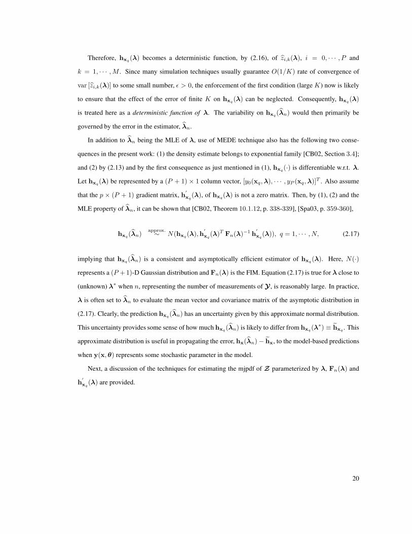
Therefore, hxq(λ) becomes a deterministic function, by (2.16), of zi,k(λ), i = 0, · · · , P and

k = 1, · · · ,M . Since many simulation techniques usually guarantee O(1/K) rate of convergence of

var [zi,k(λ)] to some small number, ǫ > 0, the enforcement of the first condition (large K) now is likely

to ensure that the effect of the error of finite K on hxq(λ) can be neglected. Consequently, hxq(λ)

is treated here as a deterministic function of λ. The variability on hxq(λn) would then primarily be

governed by the error in the estimator, λn.

In addition to λn being the MLE of λ, use of MEDE technique also has the following two conse-

quences in the present work: (1) the density estimate belongs to exponential family [CB02, Section 3.4];

and (2) by (2.13) and by the first consequence as just mentioned in (1), hxq(·) is differentiable w.r.t. λ.

Let hxq(λ) be represented by a (P + 1) × 1 column vector, [y0(xq,λ), · · · , yP (xq,λ)]T . Also assume

that the p × (P + 1) gradient matrix, h′

xq(λ), of hxq(λ) is not a zero matrix. Then, by (1), (2) and the

MLE property of λn, it can be shown that [CB02, Theorem 10.1.12, p. 338-339], [Spa03, p. 359-360],

hxq(λn)approx.∼ N(hxq(λ),h

′

xq(λ)T Fn(λ)−1 h

′

xq(λ)), q = 1, · · · , N, (2.17)

implying that hxq(λn) is a consistent and asymptotically efficient estimator of hxq(λ). Here, N(·)

represents a (P +1)-D Gaussian distribution and Fn(λ) is the FIM. Equation (2.17) is true for λ close to

(unknown) λ∗ when n, representing the number of measurements of Y , is reasonably large. In practice,

λ is often set to λn to evaluate the mean vector and covariance matrix of the asymptotic distribution in

(2.17). Clearly, the prediction hxq(λn) has an uncertainty given by this approximate normal distribution.

This uncertainty provides some sense of how much hxq(λn) is likely to differ from hxq(λ∗) ≡ hxq . This

approximate distribution is useful in propagating the error, hx(λn) − hx, to the model-based predictions

when y(x,θ) represents some stochastic parameter in the model.

Next, a discussion of the techniques for estimating the mjpdf of Z parameterized by λ, Fn(λ) and

h′

xq(λ) are provided.

20

2.3 Estimations of the mjpdf of the nKL Vector, the Fisher Infor-

mation Matrix and the Gradient Matrix

Since the mjpdf of Z , that is parameterized by λ, is estimated by using MEDE technique, a brief dis-

cussion of this technique, its relationship to MLE and the specific estimation technique employed in the

current work are included in section 2.3.1. The estimation techniques of the FIM, Fn(λ), and the gradient

matrix, h′

xq(λ), are provided, respectively, in sections 2.3.4 and 2.3.5.

2.3.1 Multivariate Joint Probability Density Function of the nKL Vector

Given a finite data set, a density estimation technique consists of evaluating a pdf that is consistent, in

some sense, with the data set. In general, this is an ill-posed problem because the solution is non-unique

since many (possibly infinite) probability density functions can generate this specific data set with positive

probability. The problem becomes more challenging in a multidimensional setting given the large amount

of data required to estimate the density. If a priori information is available about the characteristics and

functional form of the density, parametric estimation techniques making use of this information, can

significantly reduce the amount of data required for density estimation. However, a priori or additional

information may not always be available in many cases, and nonparametric density estimation techniques

[Ize91] become useful in such situations. Kernel density estimation (KDE) techniques are some of the

best-developed techniques in the literature and have been well-adapted to the multivariate case [Sco92,

Chapter 6]. However, it suffers from a few drawbacks, for example, it usually shows spurious lobes and

bumps in the estimates of the density functions (see Figure 2.5 showing a few bumps and lobes near the

tail of the marpdf, based on measurement data, estimated by using KDE technique) and is computationally

demanding for multivariate problems.

In the current work, an estimate, pZ(Z) ≡ pZ(z1, z2, · · · , zM ), of the mjpdf of Z is obtained by

relying on the MEDE technique [SKR00, Wu03] that is based on the MaxEnt principle [Sha48, Jay57a,

Jay57b, KK92]. Here, ‘entropy’ can be treated as a quantitative measure of uncertainty. The MaxEnt

principle essentially states that in the absence of a priori knowledge about the probability model of the

random quantity under consideration, a PDF should be selected that is most consistent with the available

information contained in the given data set and closest to the uniform distribution (since uniform distri-

bution has maximum entropy or uncertainty on a bounded support in absence of a priori knowledge) in

21

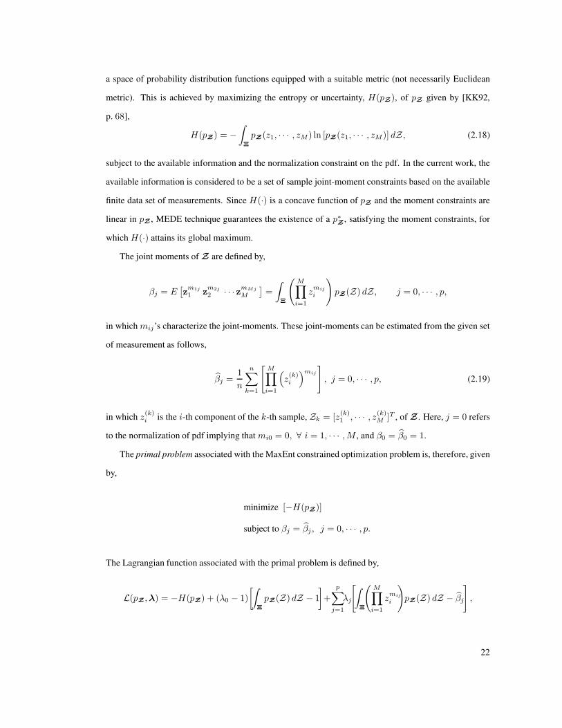
a space of probability distribution functions equipped with a suitable metric (not necessarily Euclidean

metric). This is achieved by maximizing the entropy or uncertainty, H(pZ), of pZ given by [KK92,

p. 68],

H(pZ) = −∫

Ξ

pZ(z1, · · · , zM ) ln [pZ(z1, · · · , zM )] dZ, (2.18)

subject to the available information and the normalization constraint on the pdf. In the current work, the

available information is considered to be a set of sample joint-moment constraints based on the available

finite data set of measurements. Since H(·) is a concave function of pZ and the moment constraints are

linear in pZ , MEDE technique guarantees the existence of a p∗Z , satisfying the moment constraints, for

which H(·) attains its global maximum.

The joint moments of Z are defined by,

βj = E[z

m1j

1 zm2j

2 · · · zmMj

M

]=

∫

Ξ

(M∏

i=1

zmij

i

)pZ(Z) dZ, j = 0, · · · , p,

in which mij’s characterize the joint-moments. These joint-moments can be estimated from the given set

of measurement as follows,

βj =1

n

n∑

k=1

[M∏

i=1

(z(k)i

)mij

], j = 0, · · · , p, (2.19)

in which z(k)i is the i-th component of the k-th sample, Zk = [z

(k)1 , · · · , z(k)

M ]T , of Z . Here, j = 0 refers

to the normalization of pdf implying that mi0 = 0, ∀ i = 1, · · · ,M , and β0 = β0 = 1.

The primal problem associated with the MaxEnt constrained optimization problem is, therefore, given

by,

minimize [−H(pZ)]

subject to βj = βj , j = 0, · · · , p.

The Lagrangian function associated with the primal problem is defined by,

L(pZ ,λ) = −H(pZ) + (λ0 − 1)

[∫

Ξ

pZ(Z) dZ − 1

]+

p∑

j=1

λj

[∫

Ξ

(M∏

i=1

zmij

i

)pZ(Z) dZ − βj

],

22

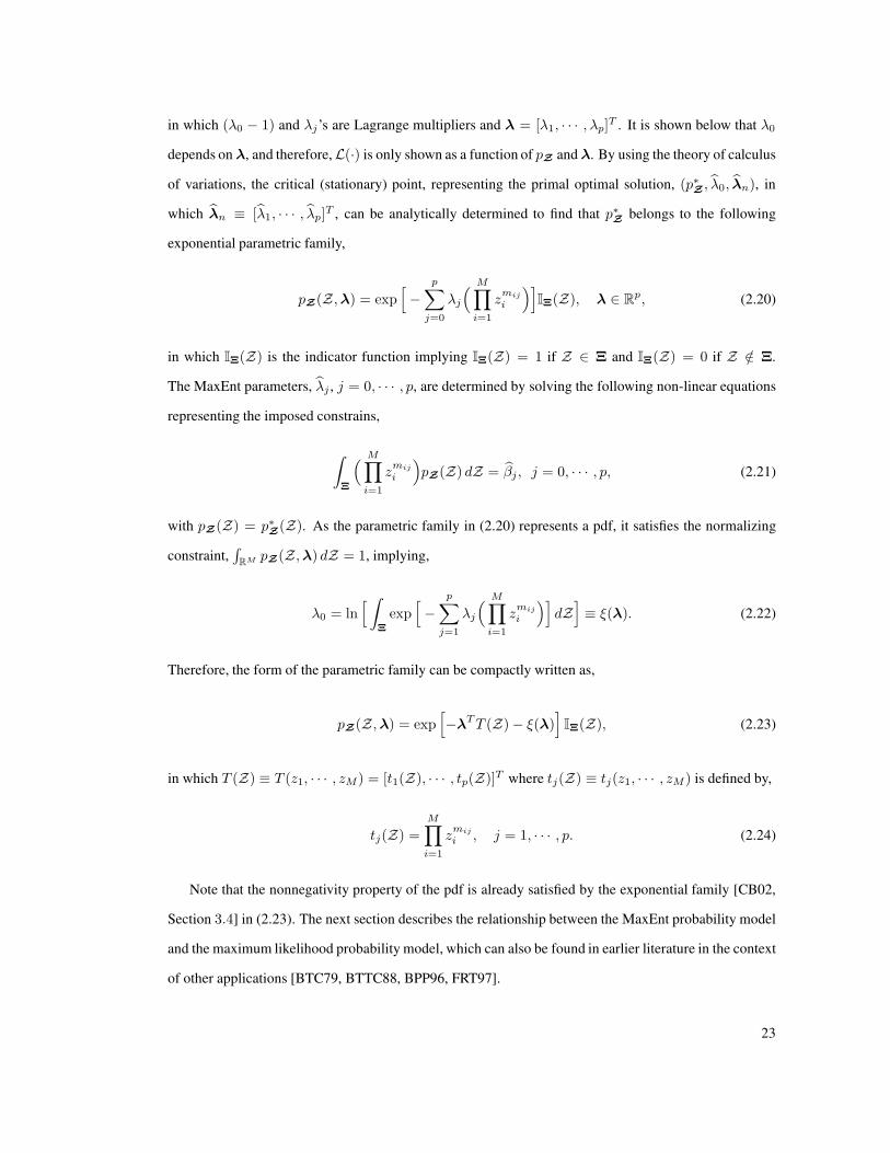
in which (λ0 − 1) and λj’s are Lagrange multipliers and λ = [λ1, · · · , λp]T . It is shown below that λ0

depends on λ, and therefore,L(·) is only shown as a function of pZ and λ. By using the theory of calculus

of variations, the critical (stationary) point, representing the primal optimal solution, (p∗Z , λ0, λn), in

which λn ≡ [λ1, · · · , λp]T , can be analytically determined to find that p∗Z belongs to the following

exponential parametric family,

pZ(Z,λ) = exp[−

p∑

j=0

λj

( M∏

i=1

zmij

i

)]IΞ(Z), λ ∈ R

p, (2.20)

in which IΞ(Z) is the indicator function implying IΞ(Z) = 1 if Z ∈ Ξ and IΞ(Z) = 0 if Z /∈ Ξ.

The MaxEnt parameters, λj , j = 0, · · · , p, are determined by solving the following non-linear equations

representing the imposed constrains,

∫

Ξ

( M∏

i=1

zmij

i

)pZ(Z) dZ = βj , j = 0, · · · , p, (2.21)

with pZ(Z) = p∗Z(Z). As the parametric family in (2.20) represents a pdf, it satisfies the normalizing

constraint,∫

RM pZ(Z,λ) dZ = 1, implying,

λ0 = ln[ ∫

Ξ

exp[−

p∑

j=1

λj

( M∏

i=1

zmij

i

)]dZ]≡ ξ(λ). (2.22)

Therefore, the form of the parametric family can be compactly written as,

pZ(Z,λ) = exp[−λTT (Z) − ξ(λ)

]IΞ(Z), (2.23)

in which T (Z) ≡ T (z1, · · · , zM ) = [t1(Z), · · · , tp(Z)]T where tj(Z) ≡ tj(z1, · · · , zM ) is defined by,

tj(Z) =

M∏

i=1

zmij

i , j = 1, · · · , p. (2.24)

Note that the nonnegativity property of the pdf is already satisfied by the exponential family [CB02,

Section 3.4] in (2.23). The next section describes the relationship between the MaxEnt probability model

and the maximum likelihood probability model, which can also be found in earlier literature in the context

of other applications [BTC79, BTTC88, BPP96, FRT97].

23

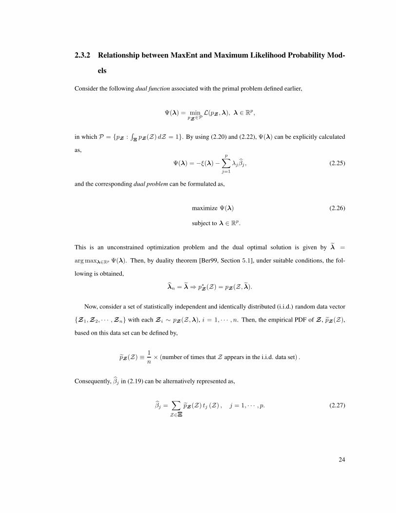
2.3.2 Relationship between MaxEnt and Maximum Likelihood Probability Mod-

els

Consider the following dual function associated with the primal problem defined earlier,

Ψ(λ) = minpZ∈P

L(pZ ,λ), λ ∈ Rp,

in which P = {pZ :∫ΞpZ(Z) dZ = 1}. By using (2.20) and (2.22), Ψ(λ) can be explicitly calculated

as,

Ψ(λ) = −ξ(λ) −p∑

j=1

λj βj , (2.25)

and the corresponding dual problem can be formulated as,

maximize Ψ(λ) (2.26)

subject to λ ∈ Rp.

This is an unconstrained optimization problem and the dual optimal solution is given by λ =

arg maxλ∈Rp Ψ(λ). Then, by duality theorem [Ber99, Section 5.1], under suitable conditions, the fol-

lowing is obtained,

λn = λ ⇒ p∗Z(Z) = pZ(Z, λ).

Now, consider a set of statistically independent and identically distributed (i.i.d.) random data vector

{Z1,Z2, · · · ,Zn} with each Z i ∼ pZ(Z,λ), i = 1, · · · , n. Then, the empirical PDF of Z , pZ(Z),

based on this data set can be defined by,

pZ(Z) ≡ 1

n× (number of times that Z appears in the i.i.d. data set) .

Consequently, βj in (2.19) can be alternatively represented as,

βj =∑

Z∈Ξ

pZ(Z) tj (Z) , j = 1, · · · , p. (2.27)

24

Next, stacking the vectors of this random data in Zn, i.e., Zn = [ZT1 , · · · ,ZT

n ]T , the mjpdf of Zn is

given by pZn(Zn |λ) =

∏ni=1 pZi

(Zi,λ) in which pZi(Zi,λ) ≡ pZ(z

(i)1 , · · · , z(i)

M ,λ). The likelihood

function of λ is then defined by ℓ(λ | Zn) = pZn(Zn | λ). Finally, by using (2.25) and (2.27), the

associated log-likelihood function can be shown to be given by,

ln ℓ(λ |Zn) = nΨ(λ).

This facts implies that maximizing the log-likelihood function is equivalent to maximizing the dual func-

tion as defined by the dual problem in (2.26). With this interpretation, it can be stated that the MaxEnt

mjpdf of Z, p∗Z(z1, · · · , zM ), is the mjpdf in the parametric family, {pZ(Z,λ),λ ∈ Rp}, that maximizes

the log-likelihood function of λ. This appealing fact reinforces the reasoning as to why the MaxEnt prin-

ciple can be preferred in estimating the mjpdf of Z .

It is shown later in section 2.3.4 (see (2.33)) that the (r, s)-th element of the Hessian matrix of

ln ℓ(λ | Zn) is given by −n cov [tr(Z)ts(Z)], r, s = 1, · · · , p. If the moment constraints in (2.21)

are imposed such that {1, t1(Z), · · · , tp(Z)} is a linearly independent set, then the covariance matrix,

cov [tr(Z)ts(Z)], is always positive definite implying that the Hessian matrix is always negative definite.

Thus, ln ℓ(· |Zn) is a strictly concave function of λ guaranteeing the existence of λn for which ln ℓ(· |Zn)

attains the global maximum value conforming to the fact that H(·) has a global maxima at p∗Z .

2.3.3 MEDE Technique and Some Remarks on the Form of pZ(Z)

Based on (2.23), the estimate of the mjpdf of Z is obtained as,

p∗Z(Z) ≡ pZ(Z) = exp[−λTT (Z)− ξ(λ)

]IΞ(Z), (2.28)

in which λj , the elements of λ, are obtained by solving the following set of nonlinear equations,

∫

Ξ

tj(Z) exp[−λTT (Z)− ξ(λ)

]dZ = βj , j = 1, · · · , p. (2.29)

Here, βj are the sample joint-moments computed by (2.19), and ξ(λ) is given by,

ξ(λ) = ln

(∫

Ξ

exp[−λTT (Z)

]dZ). (2.30)

25

The set of equations in (2.29) forms a set of p nonlinear equations in p unknowns, λj’s. The MaxEnt

probability model in (2.28) is then obtained by solving this set of nonlinear equations that involves com-

putation of M -dimensional integrations as shown in (2.29) and (2.30).

For a scalar random variable case, a numerical technique has been developed that uses a sequential

updating procedure [Wu03] in conjunction with the Newton-Raphson algorithm. The sequential updating

method imposes the sample moment constraints one at a time from the lower order moments to the higher

order moments, and updates the pdf sequentially.

The implementation of the Newton-Raphson algorithm requires an initial guess for λ to which both

the convergence and the rate of convergence of the algorithm are highly sensitive. Furthermore, in the

multivariate case, a difficulty arises due to the fact that several moments are associated with a given order.

Consequently, the additional information in a set of moments having the same given order (‘additional’ in

the sense that the information in addition to that contained in the set of moments having order lower than

the given order) are distributed among those moments in a disjoint fashion. The primary difficulty in such

cases, therefore, becomes the issue of choosing a reasonable initial guess for λ. The sequential updating

method in conjunction with Newton-Raphson method is likely to fail in such a situation. Therefore, a

method, that does not depend much on the choice of the initial guess for λ, would be more useful. In the

present work, the Levenberg-Marquardt method, a nonlinear least squares technique, as used in earlier

literature [SKR00] in the context of a scalar-valued random variable case is used for this purpose. This

method may suffer from a slower convergence rate in the event that a good initial guess is available for the

Newton-Raphson method. The true potential of the Levenberg-Marquardt algorithm is, however, realized

in the absence of such an initial guess.

To implement the Levenberg-Marquardt technique, the residuals of (2.29) are written as follows by

using (2.30),

Rj = 1 −

∫

Ξ

tj(Z) exp[−λTT (Z)

]dZ

βj

∫

Ξ

exp[−λTT (Z)

]dZ

, j = 1, · · · , p. (2.31)

The unknown parameter vector, λ, can be evaluated by using the Levenberg-Marquardt method with

or without the sequential updating method by minimizing the sum of squares of the residuals in (2.31).

The interesting feature of the sequential updating method, however, is that it generates a sequence of λ

(i.e., the mjpdf of Z) associated with the sequential activation of the joint-moment constraints. In the

26

present work, a hybrid MATLAB-FORTRAN program is written to perform this task. The main program

written in MATLAB calls a FORTRAN numerical integration subroutine to speed up the process. The

MATLAB command, lsqnonlin, is used to perform the nonlinear least-square technique with the

Levenberg-Marquardt method option ‘On’ to evaluate λ. The vector, λ, would be treated further as the

model parameter that encompasses all the information contained in the measurements of Y . Denote the

estimated model parameters collectively by λn = [λ1, · · · , λp]T .

It should be noted here that λn is a random column vector with randomness primarily being induced

by the measurements of Z (i.e., of Y). There also exist other factors, for example, measurement error,

numerical error induced by the numerical method employed for solving the set of nonlinear equations

etc., affecting the estimation of λ. However, the effects of these factors are assumed to be within accept-

able tolerance. It is clear that the true value, λ∗, of λ is not known. Once the parameter λ is spec-

ified, an estimate of the mjpdf of Z is known precisely by (2.28). Denote the associated joint PDF

by MaxEPD(Z,λ) in which MaxEPD stands for MAXimum-Entropy joint Probability Distribution. On

p. 16, the estimate of the PDF of Z , in the context of the current work, refers to MaxEPD(Z,λ) implying

that PZ (Z) ≡ MaxEPD(Z,λ).

2.3.4 Computation of the Fisher Information Matrix, Fn(λ)

An estimate of the FIM as required in (2.17) is provided in this section. Consider a sequence of i.i.d.

random data vectors, {Z1,Z2, · · · ,Zn}, with each Zv ∼ MaxEPD(Z,λ), v = 1, · · · , n. The mjpdf of

Zn = [ZT1 , · · · ,ZT

n ]T is given by,

pZn(Zn |λ) =

n∏

v=1

pZv(Zv).

Consider the p× p FIM, Fn(λ), given by [Spa03, Section 13.3.2],

Fn(λ) ≡ E

[∂ ln ℓ(λ |Zn)

∂λ· ∂ ln ℓ(λ |Zn)

∂λT

∣∣∣∣λ]

= −E[∂2 ln ℓ(λ |Zn)

∂λ ∂λT

∣∣∣∣λ]. (2.32)

Here, in a general case, the equality, ‘=’, is followed [Spa03, p. 352-353] by assuming that ln ℓ(· |Zn)

is twice differentiable w.r.t. λ and the regularity conditions [CB02, Section 10.6.2] hold for ℓ. Since pZ

belongs to an exponential family [CB02, Section 3.4], the equality, ‘=’, in (2.32) holds true in the current

27

context (see also [CB02, Section 2.4 and Lemma 7.3.11]). The log-likelihood function, in the present

work, can be explicitly computed and is shown below,

ln ℓ(λ |Zn) = ln [pZn(Zn |λ)] = −n[ξ(λ) +

p∑

j=1

λj

{1

n

n∑

v=1

(M∏

i=1

(z(v)i

)mij

)}].

It is also straightforward to compute the second derivative of ln ℓ(· |Zn) w.r.t. the elements, λr and

λs, r, s = 1, · · · , p, of λ, and the second derivative can be shown to be given by,

∂2 ln ℓ(λ |Zn)

∂λr ∂λs= −n cov [tr(Z)ts(Z)] , (2.33)

in which Z ∼ MaxEPD(Z,λ). The specific value of interest for λ here is λn. It should also be noted that,

by the definition of tj(Z) in (2.24), a few of these covariance terms should already be known by the right-

hand-side of the imposed moment constraints as defined earlier by (2.21) or (2.29). This is particularly

expected to happen for low values of r and s and consequently, in those cases, it is not required to evaluate

the M -dimensional integration over Ξ required for the computation of cov [tr(Z)ts(Z)]. Some of the

elements of the upper diagonal block of Fn(λn) would, therefore, be known and the rest of the elements

unknown implying that Fn(λn) can be divided into known and unknown parts.

Since the (r, s)-th element of Fn(λn) is given by n cov [tr(Z)ts(Z)] by (2.32)-(2.33), the FIM can be

computed by estimating these covariance terms based on pZ(Z) in (2.28) with λ = λn. The associated

multidimensional integration can be carried out by employing a numerical integration technique or a

simulation technique. The covariance terms associated with the elements of the known part need not be

computed again since these elements are already known.

2.3.5 Computation of the Gradient Matrix, h′

xq(λ)

In this section, estimate of the gradient matrix as required in (2.17) is considered. Denote the i-th col-

umn of h′

xq(λ) by ∂yi−1(xq,λ)/∂λ, i = 1, · · · , (P + 1), that is a p × 1 column vector of elements

∂yi−1(xq,λ)/∂λj , j = 1, · · · , p. Clearly, this column vector can be determined by using (2.16) as

follows,

∂yi(xq,λ)

∂λ=

M∑

k=1

vqk ak gi,k(λ), i = 0, · · · , P, and q = 1, · · · , N. (2.34)

28

Here, the gradient vector, gi,k(λ) ≡ ∂zi,k(λ)/∂λ, is a p × 1 column vector of elements, gi,k(λ) ≡

∂zi,k(λ)/∂λj , j = 1, · · · , p. By (2.14), the gradient vector, gi,k(λ), essentially is an estimator of the

vector given by,

gi,k(λ) ≡ ∂zi,k(λ)

∂λ=

1

E[Υ2

i (ξ)] ∂Eλ [zkΥi(Z)]

∂λ,

i = 0, · · · , P,

k = 1, · · · ,M .

(2.35)

This can be calculated analytically by differentiating the resulting expression of (2.13) w.r.t. λ and substi-

tuting the result in (2.35). The integration and differentiation can be performed numerically. Another way

to obtain an approximation of gi,k(λ) is to employ the classical finite-difference (FD) technique [Spa03,

Section 6.3]. The two-sided FD approximation of gi,k(λ) for use with (2.34) is given by,

gi,k(λ) ≈ gi,k(λ) =

zi,k(λ + c11) − zi,k(λ − c11)

2c...

zi,k(λ + c1p) − zi,k(λ − c1p)

2c

, (2.36)

in which gi,k(λ) is the two-sided FD approximation of gi,k(λ), 1j denotes a p× 1 column vector with 1

at the j-th place and 0 elsewhere and c > 0 is a small scalar.

The classical FD approximation technique requires 2p evaluations of zi,k(·). Since the number of

evaluations of zi,k(·) grows with p for FD technique, simultaneous perturbation (SP) gradient approxima-

tion technique, introduced in the field of stochastic optimization [Spa92] (see [Spa03, Section 7.2] for a

relatively simpler version of [Spa92]), might be useful for large p. This technique calls for averaging the

gradient approximation over a multiple number of iterations and the number of estimation is only two per

iteration regardless of the dimension of p. However, the FD approximation generally provides a superior

approximation of gi,k(λ) than its SP counterpart but the computational savings of SP technique might be

a significant benefit for large p.

2.4 Numerical Illustration and Discussions

Consider a second-order random process, y(x,θ), representing some random system parameter, evolved

over a rectangular spatial domain, D, of size 1.0 × 0.8 in appropriate length scale.

29

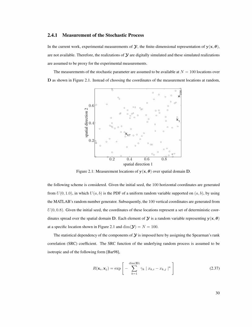
2.4.1 Measurement of the Stochastic Process

In the current work, experimental measurements of Y , the finite-dimensional representation of y(x,θ),

are not available. Therefore, the realizations of Y are digitally simulated and these simulated realizations

are assumed to be proxy for the experimental measurements.

The measurements of the stochastic parameter are assumed to be available at N = 100 locations over

D as shown in Figure 2.1. Instead of choosing the coordinates of the measurement locations at random,

spat

ial

dir

ecti

on

2

spatial direction 1

x

x

x

0.2

0.2

0.4

0.4

0.6

0.6 0.8

1

67

100

Figure 2.1: Measurement locations of y(x,θ) over spatial domain D.

the following scheme is considered. Given the initial seed, the 100 horizontal coordinates are generated

from U(0, 1.0), in which U(a, b) is the PDF of a uniform random variable supported on (a, b), by using

the MATLAB’s random number generator. Subsequently, the 100 vertical coordinates are generated from

U(0, 0.8). Given the initial seed, the coordinates of these locations represent a set of deterministic coor-

dinates spread over the spatial domain D. Each element of Y is a random variable representing y(x,θ)

at a specific location shown in Figure 2.1 and dim(Y) = N = 100.

The statistical dependency of the components of Y is imposed here by assigning the Spearman’s rank

correlation (SRC) coefficient. The SRC function of the underlying random process is assumed to be

isotropic and of the following form [Bar98],

R(xi,xj) = exp

[−

dim(D)∑

k=1

γk | xk,i − xk,j |κ]

(2.37)

30

in which R(xi,xj) is the SRC between two random variables associated with the locations having coor-

dinates xi and xj , γk, k = 1, · · · , dim (D), is the inverse of the correlation length along the spatial

direction k, | xk,i − xk,j | is the absolute value of (xk,i − xk,j) in which xk,i and xk,j are, respectively,

the k-th coordinates of xi and xj and κ is a constant. In the present case, dim (D) = 2 and it is assumed

that γk = 0.5, k = 1, 2, and κ = 2. The marginal PDF of yq , q = 1, · · · , N , is assumed to be lognormal

with its pdf being given by,

fyq(y) =

1

ygµq,σq (ln y) if y > 0,

0 if y ≤ 0,

in which gµq,σq(x) = [1/(√

2πσq)] exp[(x − µq)/(2σ2q)] is the Gaussian density and µq and σ2

q are,

respectively, mean and variance of the associated Gaussian random variable and given by,

µq = lnµyq −1

2ln

(σ2yq

µ2yq

+ 1

),

σ2q = ln

(σ2yq

µ2yq

+ 1

),

(2.38)

in which µyq and σ2yq

are, respectively, mean and variance of yq .

N

Sta

tist

ics

ofy

q

µyq

σyq

0 2040 40

60

60

80

80

100

100

120

140

160

180

200

Figure 2.2: Statistics of yq , q = 1, · · · , N .

To ensure the non-stationary characteristic of the random process, different values of mean are

assigned to each yq . Like the coordinates of the 100 locations are generated given the initial seed, the 100

31

mean values of yq are also generated from U(0.85D, 1.15D) in which D is assumed to be 168. Coeffi-

cient of variation is assumed to be 0.3 for all yq . The values of µyq and σyq thus selected are depicted

in Figure 2.2. Denote the N × 1 column vector consisting of {µyq}Nq=1 by µy = [µy1 , · · · , µyN ]T and

similarly the column vector of {σyq}Nq=1 by σy = [σy1 , · · · , σyN ]T .

The N × N SRC matrix, Ryy, of Y is computed by using (2.37). The (i, j)-th element, ρs(yi,yj),

of Ryy is calculated by substituting xi and xj coordinates in (2.37). The SRC matrix is same [KC06,

Section 3.2.2] for both the non-Gaussian vector, Y , and its underlying correlated Gaussian vector whose

elements follow the standard normal distribution, N(0, 1). The SRC matrix, Ryy, is then transformed to

the Pearson’s correlation coefficient (PCC) matrix (the ‘usual’ correlation coefficient matrix) of the under-

lying correlated Gaussian vector by using the following relation proposed by Pearson in 1904 [KC06, p. 51

and p. 75-77],

ρij = 2 sin(π

6ρs(yi,yj)

), i, j = 1, · · · , N, (2.39)

in which ρij is the (i, j)-th element of the PCC matrix. This PCC matrix, [ρij ], however, does not match

with the PCC matrix of Y . Based on [ρij ], the underlying correlated Gaussian vector is simulated by

using its KL expansion. In this example, the number of terms retained in the KL expansion is 3 because

99% of the variance of the underlying correlated Gaussian vector is contributed by the 3 dominant KL

random variables associated with the largest 3 eigenvalues of [ρij ]. Subsequently, the realizations of the

underlying correlated Gaussian vector thus generated by using its KL expansion are shifted and scaled to

enforce the required mean and variance vector whose elements are given by (2.38). The realizations of

this Gaussian vector are finally transformed into the realizations of Y by using the target marginal PDF of

yq by having recourse to the inverse-transform method, Y = exp [X ], in which X is theN×1 correlated

Gaussian vector whose mean vector, variance vector and correlation matrix are, respectively, given by

[µ1, · · · , µN ]T , [σ21 , · · · , σ2

N ]T and [ρij ].

In this numerical illustration, an additive Gaussian noise is also applied to the realizations of pure

Y , say Y(pure), to obtain noisy (as usually the case in practice) realizations of Y as Y = Y(pure) +

N(0, diag(0.04σy)), in which N(·) represents an N -D Gaussian vector, 0 is a N × 1 column vector of

zeros representing the mean vector and diag(0.04σy) is a diagonal matrix representing the covariance

matrix whose i-th diagonal entry is 0.04σyi , i = 1, · · · , N . These noisy realizations of Y would be

treated further as the experimental measurements.

32

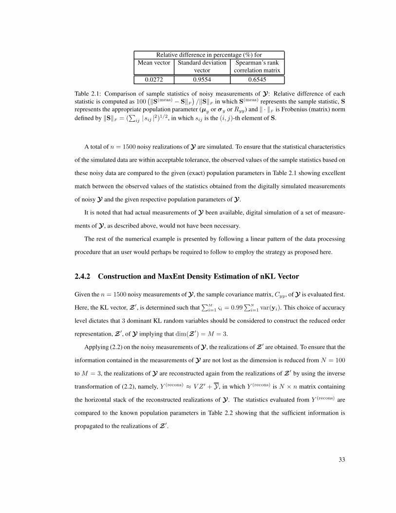
Relative difference in percentage (%) for

Mean vector Standard deviation Spearman’s rank

vector correlation matrix

0.0272 0.9554 0.6545

Table 2.1: Comparison of sample statistics of noisy measurements of Y : Relative difference of each

statistic is computed as 100(‖S(meas) − S‖F

)/‖S‖F in which S(meas) represents the sample statistic, S

represents the appropriate population parameter (µy or σy or Ryy) and ‖ · ‖F is Frobenius (matrix) norm

defined by ‖S‖F = (∑

ij |sij |2)1/2, in which sij is the (i, j)-th element of S.

A total of n = 1500 noisy realizations of Y are simulated. To ensure that the statistical characteristics

of the simulated data are within acceptable tolerance, the observed values of the sample statistics based on

these noisy data are compared to the given (exact) population parameters in Table 2.1 showing excellent

match between the observed values of the statistics obtained from the digitally simulated measurements

of noisy Y and the given respective population parameters of Y .

It is noted that had actual measurements of Y been available, digital simulation of a set of measure-

ments of Y , as described above, would not have been necessary.

The rest of the numerical example is presented by following a linear pattern of the data processing

procedure that an user would perhaps be required to follow to employ the strategy as proposed here.

2.4.2 Construction and MaxEnt Density Estimation of nKL Vector

Given the n = 1500 noisy measurements of Y , the sample covariance matrix,Cyy , of Y is evaluated first.

Here, the KL vector, Z′, is determined such that

∑M

i=1 ςi = 0.99∑N

i=1 var(yi). This choice of accuracy

level dictates that 3 dominant KL random variables should be considered to construct the reduced order

representation, Z ′, of Y implying that dim(Z ′) = M = 3.

Applying (2.2) on the noisy measurements of Y , the realizations of Z′ are obtained. To ensure that the

information contained in the measurements of Y are not lost as the dimension is reduced from N = 100

to M = 3, the realizations of Y are reconstructed again from the realizations of Z′ by using the inverse

transformation of (2.2), namely, Y (recons) ≈ V Z ′ + Y , in which Y (recons) is N × n matrix containing

the horizontal stack of the reconstructed realizations of Y . The statistics evaluated from Y (recons) are

compared to the known population parameters in Table 2.2 showing that the sufficient information is

propagated to the realizations of Z′.

33

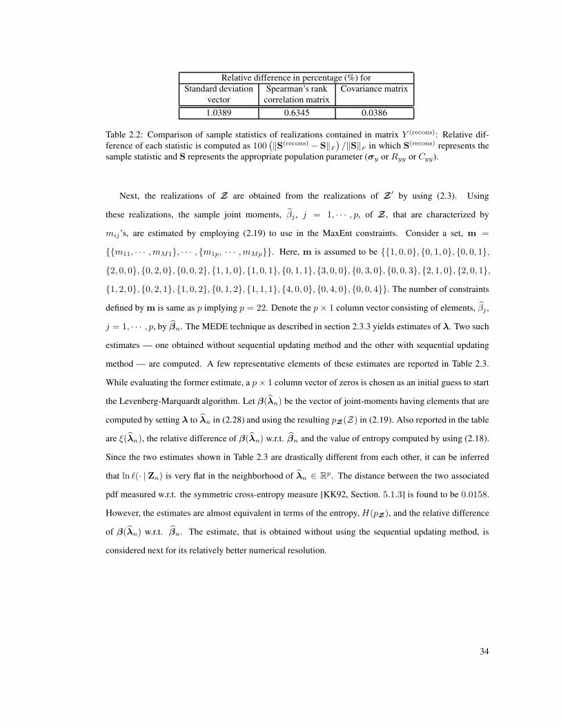
Relative difference in percentage (%) for

Standard deviation Spearman’s rank Covariance matrix

vector correlation matrix

1.0389 0.6345 0.0386

Table 2.2: Comparison of sample statistics of realizations contained in matrix Y (recons): Relative dif-

ference of each statistic is computed as 100(‖S(recons) − S‖F

)/‖S‖F in which S(recons) represents the

sample statistic and S represents the appropriate population parameter (σy or Ryy or Cyy).

Next, the realizations of Z are obtained from the realizations of Z′ by using (2.3). Using

these realizations, the sample joint moments, βj , j = 1, · · · , p, of Z , that are characterized by

mij’s, are estimated by employing (2.19) to use in the MaxEnt constraints. Consider a set, m =

{{m11, · · · ,mM1}, · · · , {m1p, · · · ,mMp}}. Here, m is assumed to be {{1, 0, 0}, {0, 1, 0}, {0, 0, 1},

{2, 0, 0}, {0, 2, 0}, {0, 0, 2}, {1, 1, 0}, {1, 0, 1}, {0, 1, 1}, {3, 0, 0}, {0, 3, 0}, {0, 0, 3}, {2, 1, 0}, {2, 0, 1},

{1, 2, 0}, {0, 2, 1}, {1, 0, 2}, {0, 1, 2}, {1, 1, 1}, {4, 0, 0}, {0, 4, 0}, {0, 0, 4}}. The number of constraints

defined by m is same as p implying p = 22. Denote the p× 1 column vector consisting of elements, βj ,

j = 1, · · · , p, by βn. The MEDE technique as described in section 2.3.3 yields estimates of λ. Two such

estimates — one obtained without sequential updating method and the other with sequential updating

method — are computed. A few representative elements of these estimates are reported in Table 2.3.

While evaluating the former estimate, a p× 1 column vector of zeros is chosen as an initial guess to start

the Levenberg-Marquardt algorithm. Let β(λn) be the vector of joint-moments having elements that are

computed by setting λ to λn in (2.28) and using the resulting pZ(Z) in (2.19). Also reported in the table

are ξ(λn), the relative difference of β(λn) w.r.t. βn and the value of entropy computed by using (2.18).

Since the two estimates shown in Table 2.3 are drastically different from each other, it can be inferred

that ln ℓ(· | Zn) is very flat in the neighborhood of λn ∈ Rp. The distance between the two associated

pdf measured w.r.t. the symmetric cross-entropy measure [KK92, Section. 5.1.3] is found to be 0.0158.

However, the estimates are almost equivalent in terms of the entropy, H(pZ), and the relative difference

of β(λn) w.r.t. βn. The estimate, that is obtained without using the sequential updating method, is

considered next for its relatively better numerical resolution.

34

Quantity Without sequential With sequential

updating method updating method

λ1 -74.9164 -85.4308...

......

λ4 107.1809 107.7935...

......

λ22 -41.7542 0

ξ(λn) 29.1208 41.0928

100‖β(λn)−βn‖

‖βn‖0.0054 0.0057

H(pZ) -1.9721 -1.9725

Table 2.3: λn, ξ(λn), relative difference of joint moment vector and H(pZ).

2.4.3 Simulation of the nKL vector and Estimation of the Fisher Information

Matrix

Having estimated λn by using MEDE technique, the next step is to estimate Fn(λn). Here, Fn(λn) is

computed by using a numerical integration technique as well as estimated by using a sampling technique.

For the sampling-based estimate, the independent samples of Z are generated by using M-H MCMC

algorithm [Spa03, Section 16.2]. In this algorithm, given the k-th state, Zk, of Z, the candidate point, W ,

is generated according to a given proposal PDF. The following proposal PDF is considered for q(· | Zk)

for the present example,

q(W |Zk) ∼ UM (W − δ1M ,W + δ1M ) , (2.40)

in which UM (a,b) is a M -fold uniform PDF in which a and b areM -D vectors whose elements, respec-

tively, represent the lower and upper bounds of the respective one-dimensional uniform random variable,

δ is a positive constant and 1M is an M -D vector of 1s. Here, δ is assumed to be 0.3.

It must be noted that because Z has a finite support Ξ = [0 1]M

, the support, supp (W |Zk), of

W | Zk (and therefore, also the height of the proposal pdf in (2.40) to enforce the volume of the PDF to

be unity) must be continuously changing during the runs of MCMC to guarantee the generation of W

within the supp (W |Zk) ⊂ Ξ. The conditional PDF, q(· |W), of Zk is also required for M-H MCMC

algorithm. Here, Zk is the possible k-th state given the value, W , of W . The expression of q(Zk |W)

is analogous to the expression in (2.40). The support and height for q(Zk |W) also need to be changed

35

during the runs of MCMC to guarantee that supp (Zk |W) ⊂ Ξ. It essentially implies that Eq. (16.3) on

p. 441 of ref. [Spa03] cannot be reduced to the simplified version as shown on p. 442 of ref. [Spa03].

burn-in period

Eu

clid

ean

no

rmo

fm

om

ent

vec

tor MCMC simulation (2170 samples)

measurements

0 100 200 300 400 500

1.14

1.16

1.18

1.2

1.22

1.24

1.26

1.28

1.3

Figure 2.3: Euclidean norm, ‖β(MCMC)‖, of β(MCMC), representing the vector of sample joint-moments

estimated by using 2170 independent MCMC samples and shown as solid line, is compared to ‖βn‖shown as dashed line.

In M-H MCMC, a burn-in-period of 300 is considered for the present example. The 301st sample

resulting from one run of MCMC yields one sample. A total of 2170 such independent runs of MCMC

yields 2170 independent samples of Z. All the 22 sample joint-moments of Z , estimated based on

these 2170 independent samples, are found to converge to the stationary values around the respective

components of βn justifying that the burn-in-period of 300 is sufficient enough (see Figure 2.3). A total

of 950000 independent runs of MCMC is carried out to generate Ns = 950000 independent data vectors

as a proxy for Z . The mean, standard deviation, maximum and minimum values of the acceptance rate

over 950000 MCMC runs are found to be, respectively, 30.9217%, 4.0106%, 51.1628% and 1.6611%.

As indicated earlier, because of the use of MEDE technique, the 22 × 22 FIM here has an interesting

feature in the sense that it can be divided into known and unknown parts as shown in Figure 2.4. The

unknown elements of Fn(λn) is estimated by using the independent MCMC samples as simulated above.

The unknown elements of Fn(λn) is also evaluated by a direct numerical integration scheme. Denote the

later FIM by Fn(λn)(anal) and the sampling-based estimate by Fn(λn)(MCMC). The relative difference

of Fn(λn)(MCMC) w.r.t. Fn(λn)(anal) measured in terms of Frobenius norm is found to be 1.0941%.

36

Known elements = 54

1

1

4

4

8

8

12

12

16

16

20

2022

22

Figure 2.4: Fisher information matrix with known elements as marked; void part consists of unknown

elements.

2.4.4 Estimation of PC coefficients of Z and Y

To compute the estimators, {zi,k(λn)}Pi=0, defined by (2.15), a set of statistically independent standard

normal random variables, {ξi}nd

i=1, is used. The basic polynomials, Ψj(ξi), then turn out to be Hermite

polynomials given by,

Ψ0(ξi) = 1, Ψ1(ξi) = ξi,

Ψj(ξi) = ξiΨj−1(ξi) − (j − 1)Ψj−2(ξi), if j ≥ 2,(2.41)

and the variance of Ψαi(ξi) in (2.9) is given by [SG04a],

E[Ψ2

αi(ξi)

]= αi!, i = 1, · · · , nd.

The order, no, of the PC representation is considered to be 2 and the dimension, nd, as already argued,

is fixed to the value of M = 3. For computations described in this subsection, only the first K = 2170

samples of 950000 MCMC samples are considered. The mean, standard deviation, maximum and mini-

mum values of the acceptance rate over these 2170 MCMC runs are found to be, respectively, 31.1659%,

4.0184%, 46.1794% and 15.9468%. The sample joint-moment vector, β(MCMC), of Z based on these

2170 MCMC samples is compared to βn. The relative difference of β(MCMC) w.r.t. βn measured in

37

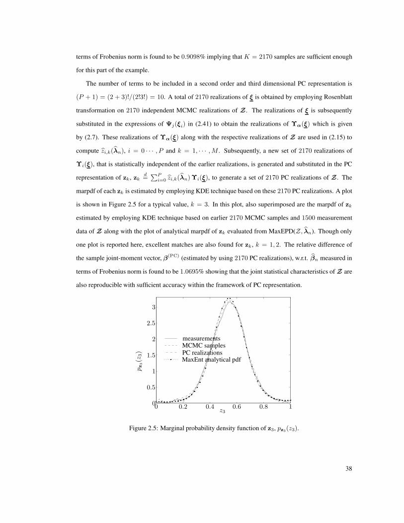
terms of Frobenius norm is found to be 0.9098% implying that K = 2170 samples are sufficient enough

for this part of the example.

The number of terms to be included in a second order and third dimensional PC representation is

(P + 1) = (2 + 3)!/(2!3!) = 10. A total of 2170 realizations of ξ is obtained by employing Rosenblatt

transformation on 2170 independent MCMC realizations of Z . The realizations of ξ is subsequently

substituted in the expressions of Ψj(ξi) in (2.41) to obtain the realizations of Υα(ξ) which is given

by (2.7). These realizations of Υα(ξ) along with the respective realizations of Z are used in (2.15) to

compute zi,k(λn), i = 0 · · · , P and k = 1, · · · ,M . Subsequently, a new set of 2170 realizations of

Υi(ξ), that is statistically independent of the earlier realizations, is generated and substituted in the PC

representation of zk, zkd=∑P

i=0 zi,k(λn)Υi(ξ), to generate a set of 2170 PC realizations of Z . The

marpdf of each zk is estimated by employing KDE technique based on these 2170 PC realizations. A plot

is shown in Figure 2.5 for a typical value, k = 3. In this plot, also superimposed are the marpdf of zk

estimated by employing KDE technique based on earlier 2170 MCMC samples and 1500 measurement

data of Z along with the plot of analytical marpdf of zk evaluated from MaxEPD(Z, λn). Though only

one plot is reported here, excellent matches are also found for zk , k = 1, 2. The relative difference of

the sample joint-moment vector, β(PC) (estimated by using 2170 PC realizations), w.r.t. βn measured in

terms of Frobenius norm is found to be 1.0695% showing that the joint statistical characteristics of Z are

also reproducible with sufficient accuracy within the framework of PC representation.

z3

pz3(z

3)

measurementsMCMC samplesPC realizationsMaxEnt analytical pdf

00 0.2 0.4 0.6 0.8

1

1

0.5

1.5

2

2.5

3

Figure 2.5: Marginal probability density function of z3, pz3(z3).

38

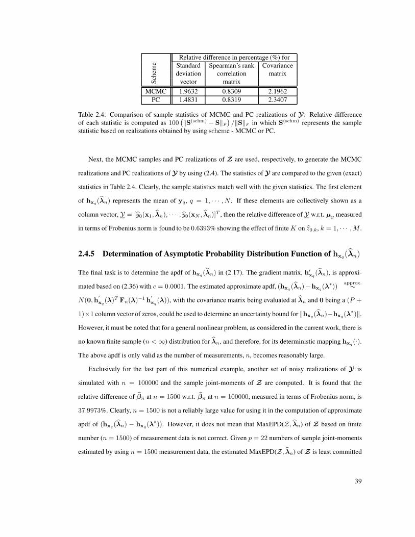
Relative difference in percentage (%) for

Standard Spearman’s rank Covariance

deviation correlation matrix

Sch

eme

vector matrix

MCMC 1.9632 0.8309 2.1962

PC 1.4831 0.8319 2.3407

Table 2.4: Comparison of sample statistics of MCMC and PC realizations of Y : Relative difference

of each statistic is computed as 100(‖S(schm) − S‖F

)/‖S‖F in which S(schm) represents the sample

statistic based on realizations obtained by using scheme - MCMC or PC.

Next, the MCMC samples and PC realizations of Z are used, respectively, to generate the MCMC

realizations and PC realizations of Y by using (2.4). The statistics of Y are compared to the given (exact)

statistics in Table 2.4. Clearly, the sample statistics match well with the given statistics. The first element

of hxq(λn) represents the mean of yq , q = 1, · · · , N . If these elements are collectively shown as a

column vector, Y = [y0(x1, λn), · · · , y0(xN , λn)]T , then the relative difference of Y w.r.t. µy measured

in terms of Frobenius norm is found to be 0.6393% showing the effect of finiteK on z0,k, k = 1, · · · ,M .

2.4.5 Determination of Asymptotic Probability Distribution Function of hxq(λn)

The final task is to determine the apdf of hxq(λn) in (2.17). The gradient matrix, h′xq

(λn), is approxi-

mated based on (2.36) with c = 0.0001. The estimated approximate apdf, (hxq (λn)−hxq(λ∗))

approx.∼

N(0,h′

xq(λ)T Fn(λ)−1 h

′

xq(λ)), with the covariance matrix being evaluated at λn and 0 being a (P +

1)×1 column vector of zeros, could be used to determine an uncertainty bound for ‖hxq(λn)−hxq(λ∗)‖.

However, it must be noted that for a general nonlinear problem, as considered in the current work, there is

no known finite sample (n <∞) distribution for λn, and therefore, for its deterministic mapping hxq(·).

The above apdf is only valid as the number of measurements, n, becomes reasonably large.

Exclusively for the last part of this numerical example, another set of noisy realizations of Y is

simulated with n = 100000 and the sample joint-moments of Z are computed. It is found that the

relative difference of βn at n = 1500 w.r.t. βn at n = 100000, measured in terms of Frobenius norm, is

37.9973%. Clearly, n = 1500 is not a reliably large value for using it in the computation of approximate

apdf of (hxq (λn) − hxq(λ∗)). However, it does not mean that MaxEPD(Z, λn) of Z based on finite

number (n = 1500) of measurement data is not correct. Given p = 22 numbers of sample joint-moments

estimated by using n = 1500 measurement data, the estimated MaxEPD(Z, λn) of Z is least committed

39

to the information not given to us. As more data arrive over time, the estimate, λn, changes. One of the

goals of the present work is to determine the confidence level of ‖hxq(λn) − hxq(λ∗)‖ as n becomes

perceivably large.

For the purpose of illustration, however, suppose that the estimated βn at n = 1500 would not

significantly change from βn at n = 1 × 1010 implying that λn at n = 1 × 1010 is almost equal to

λn at n = 1500. The FIM, Fn(λn), estimated earlier for n = 1500 can be scaled up by a factor of

(1 × 1010/1500) to approximately compute Fn(λn) at n = 1 × 1010. Hence, for n = 1 × 1010, using

the new covariance matrix, h′

xq(λ)T Fn(λ)−1 h

′

xq(λ), evaluated at λ = λ1500 with Fn(λ) being the

scaled-up Fn(λn)(anal) evaluated at n = 1500 as just mentioned, the 95% percentile confidence level of

‖hxq(λn)−hxq(λ∗)‖ is obtained as 3.4887 for a typical value, q = 1. This confidence level is computed

by simulation using 1×106 realizations. It must be again emphasized that the condition λ1500 ≈ λ1×1010

(which also implies that hxq(λ1500) ≈ hxq(λ1×1010) ≈ hxq(λ∗) ≈ hxq ) is assumed to be valid simply

for the sake of illustration and only for the last part of this numerical example when the confidence level

of the error term, ‖hxq(λn) − hxq(λ∗)‖, is determined using its approximate apdf.

2.5 Conclusions

The work presented in this chapter investigates the effects of data uncertainty on the confidence interval

of estimators of the PC coefficients of a random vector, Y , that is a finite-dimensional representation of a

non-Gaussian, non-stationary and second-order stochastic process. The KL decomposition and a scaling

transformation are employed, on a set of data measured on the random vector, to perform stochastic

model reduction. The MaxEnt mjpdf of the resulting reduced random vector (normalized KL vector,

Z) is subsequently estimated. Given the sample joint-moments estimated from the observations of Z,

the estimated mjpdf is unique and most unbiased (any deviation from this probability density function

implies a bias towards some unavailable information). The estimator, λn, of λ, that characterizes the

MaxEnt mjpdf, is computed by employing a nonlinear least-squares technique (Levenberg-Marquardt

optimization algorithm). By using the estimated mjpdf and the Rosenblatt transformation, the vector,

hxq(λn), consisting of the estimators of the PC coefficients of Y , is evaluated in order to obtain the

PC representation of Y . This PC representation approximates Y by projecting it on a finite-dimensional

space spanned by a set of orthogonal basis functions providing access to all the tools available in the

40

area of functional analysis. This is useful for many purpose, for instance, convergence analysis of the PC

representation of Y .

It is reported, in the context of the numerical example presented here, that both the estimated MaxEnt

mjpdf and the PC representation of the random vector could represent the probabilistic and statistical

characteristics of the measured data with excellent accuracy even for a finite number of measurements

which is typically the case in most practical problems. The estimator, λn, is also the MLE of λ implying

that hxq(λn) is also the MLE of hxq(λ∗) ≈ hxq representing the vector whose elements are the ‘true’

PC coefficients of the finite-dimensional representation of the stochastic process.

It should be noted that like mean, variance and other higher order joint-moments of the random pro-

cess, the PC coefficients are population parameters characterizing the random process. Clearly, the proba-

bilistic and statistical characteristics of estimators of these population parameters depend on inherent ran-

domness embodied in the available measurement data. It is reported here that hxq(λn) is also consistent

and asymptotically efficient estimator of hxq(λ∗) ≈ hxq . The associated asymptotic normal distribution,

estimated based on a large number of measurement data, is useful to determine a confidence interval as to

how much the estimates of the PC coefficients are likely to differ from the ‘true’ PC coefficients that are

typically unknown.

The computation of the asymptotic normal distribution of the PC coefficients requires estimation of

the FIM, Fn(λn). In the context of the current work, the FIM is found to have an interesting structure

where some of the elements of Fn(λn) are already known and the other elements are unknown. Because

of the use of MEDE technique resulting in a pdf from exponential family, the unknown elements can

be efficiently estimated in the current work without affecting the known elements. However, this is not

possible in other cases where all the special advantages afforded by the MEDE technique are not readily

available. A recent work [Das07] addresses this general case focusing on how the prior information, avail-

able in terms of the known elements, can be exploited to compute the better estimates for the unknown

elements.

41

Chapter 3

Polynomial Chaos Representation of

Random Field from Experimental

Measurements

Two numerical techniques are proposed to construct polynomial chaos (PC) representation of an arbitrary

second-order random vector. In the first approach, PC representation is constructed by matching a target

joint probability density function (pdf) based on the concept of conditional probability and the Rosenblatt

transformation. In the second approach, the PC representation is obtained by having recourse to the

Rosenblatt transformation and matching simultaneously a set of all target marginal pdfs and a target

Spearman’s rank correlation coefficient (SRCC) matrix. Both the techniques are applied to model a spatio-

temporal, non-stationary and non-Gaussian random temperature field, that is assumed to be a second-order

random field, by using a set of oceanographic data obtained from a shallow-water acoustics transmission

experiment [ABC+97]. The set of measurement data, observed over a finite denumerable subset of the

indexing set of the random process, is treated as a set of observed samples of a second-order random vector

that can be treated as a finite-dimensional approximation of the original random field. A complete set of

properly ordered conditional pdfs, that uniquely characterizes the target joint pdf, in the first approach and

a set of all the target marginal pdfs and the target SRCC matrix in the second approach are estimated by

using available experimental data. Digital realizations sampled from the constructed PC representations

based on both the schemes capture the observed and target statistical characteristics of the experimental

data with sufficient accuracy. The relative advantages and disadvantages of these techniques are also

highlighted.

42

3.1 Motivation and Problem Description

Unlike matching a finite set of joint higher order statistics in chapter 2, a target mjpdf or a set of tar-

get marginal probability density functions (marpdfs) along with a target correlation coefficient (corrcoef)

function are captured here by the PC representation. The use of the maximum-entropy (MaxEnt) principle

for the estimation of the target pdfs is avoided in this chapter. While this is beneficial from a computational

perspective if the construction of PC representation is the only goal, the identification of the asymptotic

probability density function (apdf) of estimators of the PC coefficients cannot be done here because of the

absence of the nice theory related to the maximum likelihood estimator (MLE) within a convex optimiza-

tion setup that was present in chapter 2 (see section 2.2.4 and section 2.3.2 for further details). Therefore,

the work in this chapter focuses more closely on the construction of the probability model (i.e., PC rep-

resentation) of a non-stationary and non-Gaussian random process by using experimental measurements,

and the associated simulation technique based on the constructed model. A brief literature survey in

the context of simulation and characterization of non-Gaussian and non-stationary random processes is

presented below to show the complete justification of carrying out the work presented here.

The most popular approach in digitally generating the realizations of non-Gaussian process is through

specifying a set of target non-Gaussian marpdfs and a target corrcoef function or spectral density func-

tion (sdf) [CN97, Gri98, DM01]. The set of target marpdfs and the target corrcoef function or sdf can

be determined by fitting a conformable set of statistics estimated from the available set of data. In syn-

thesizing the realizations through this course, it is assumed that an “underlying” Gaussian process exists

and a search technique is subsequently employed to find an “equivalent” and feasible (positive-definite)

corrcoef function of the Gaussian process. The realizations of the Gaussian process synthesized based

on the equivalent corrcoef function are then transformed to the realizations of the requisite non-Gaussian

random process. The later transformation is based on the mapping introduced earlier by Nataf in 1962

[HM00, Section 4.3]. At this stage, an additional computational budget needs to be allocated to find

the inverse functions of the target marginal probability distribution functions (marPDFs) if they are not

readily available (imagine a distribution function with multi-modal characteristics). This may often be the

case in many practical applications when the target marpdfs are estimated from the available set of data by

employing nonparametric density estimation techniques [Ize91, KPU04, DGS08], [Sco92, Chapter 6] as

employed in chapter 2. In addition to this computational overhead, counterexamples exist in the literature

43

showing that a non-Gaussian random vector with a specific target corrcoef matrix can still exist in spite

of non-existence of an underlying Gaussian random vector [GH02].

It should also be noted that there exist several other different notions of correlation in the field of sta-

tistical literatures [EMS01]. Besides the usual corrcoef, the alternative measures of statistical dependency,

that researchers had recently recourse to for characterizing non-Gaussian random processes, include

SRCC or Spearman’s rho and Kendall’s tau. The usual corrcoef, on the other hand, is known as linear or

Pearson’s correlation coefficient (PCC) in the honor of Karl Pearson who first highlighted its usefulness

as a measure of statistical dependency. A recent simulation study [HLD04, Section 12.5.2] investigates

the feasibility (positive-definiteness) of the PCC matrix of an underlying Gaussian random vector when

the statistical dependency of the non-Gaussian random vector is characterized by corrcoef matrices based

on SRCC and Kendall’s tau. It is found in their study that an underlying Gaussian vector is more likely to

exist, particularly, in a high dimensional setting, when the statistical dependency among the random vari-

able components of the non-Gaussian vector is characterized by a SRCC matrix. This feature of SRCC

has a significant practical advantage from a simulation point of view. The realizations of the Gaussian

vector, that are easy to sample digitally, can then be transformed to the realizations of the non-Gaussian

vector by using the Nataf transformation. Therefore, only the SRCC will be considered in the ensuing

discussion.

The topic on simulation of the non-Gaussian random process by specifying a set of target non-

Gaussian marpdfs and a target SRCC function has already been considered in the literature. In this case, if

the underlying Gaussian process exists, then no special search technique is required to determine the fea-

sible PCC function [CR99, GH03, PQH04], [HLD04, Section 12.5.2] facilitating computational savings

to a certain extent. However, efficient simulation still requires easy computation of the inverse functions

of the target marPDFs because of the use of Nataf transformation. Clearly, simulation techniques, based

on a target PCC/SRCC function or sdf and an underlying Gaussian process, are not computationally effi-

cient, particularly, in the case when the target set of marpdfs are estimated by employing nonparametric

techniques.

Another work [MB93, MB97], that does not assume the existence of an underlying Gaussian pro-

cess, presents an optimization technique based on Kullback-Leibler minimum cross-entropy principle for

bivariate distribution. It results in a Taylor expansion based pdf. Though, the generalization of this method

44

is theoretically feasible in higher dimensional distribution, the actual development becomes prohibitively

complicated because of the high dimensional Taylor expansion.

Recently, two new methods based on undirected graph (referred as tree and vine) have been introduced

in the literature [KC06, Chapter 4]. The technique based on a tree constructed for an N -dimensional (D)

random vector allows specification of only (N −1) elements of the SRCC matrix out ofN(N −1)/2 off-

diagonal elements. The method based on a vine relaxes this limitation, and therefore, can be theoretically

used to realize every SRCC matrix. However, the use of the later method requires knowledge of a copula

[Joe97, Nel06] that specifies the structure of the statistical dependence among the constituent random

variable components. Only a limited class of copula is investigated until now to integrate them into the

formulation based on a vine. It is unlikely that any arbitrary target SRCC matrix can be realized via this

method at its current state. Nevertheless, this method has a promising future and needs further research

attention.

The characterization of non-Gaussian random process continues to be an evolving research field draw-

ing the motivation from the practically appealing issues of estimating the underlying family of mjpdfs

from finite data [Ize91, Sco92, GH02, KPU04]. By making use of such techniques, the problem of non-

existence of an underlying Gaussian random process or the complicated Taylor expansion based pdf can

be overcome at the cost of additional computational expenses. However, advanced simulation techniques,

for example, algorithms based on Markov chain Monte Carlo (MCMC) need to be invoked to sample from

the resulting family of mjpdfs thus requiring further computational budget (as a side note, MCMC simula-

tion technique is also required to sample from the Taylor expansion based pdf). This difficulty could be a

major bottleneck particularly in the context of propagating the statistical characteristics of stochastic sys-

tem parameters to the model-based predictions if the stochastic system parameters need to be modeled as

non-Gaussian random processes. A number of studies [vdG98, PPS02, SG02a, SG02b] have been carried

out to circumvent this particular difficulty by representing the non-stationary and non-Gaussian random

processes through PC expansion [GS91]. The underlying concept of these studies is similar to the one

introduced earlier by Lancaster [Lan57], which again assumes the existence of an underlying Gaussian

process.

The work in this chapter presents two different computational techniques to estimate the probabil-

ity model of a finite-dimensional approximation, Y , of the underlying non-stationary and non-Gaussian

45

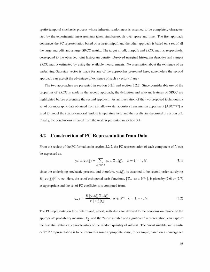
spatio-temporal stochastic process whose inherent randomness is assumed to be completely character-

ized by the experimental measurements taken simultaneously over space and time. The first approach

constructs the PC representation based on a target mjpdf, and the other approach is based on a set of all

the target marpdfs and a target SRCC matrix. The target mjpdf, marpdfs and SRCC matrix, respectively,

correspond to the observed joint histogram density, observed marginal histogram densities and sample

SRCC matrix estimated by using the available measurements. No assumption about the existence of an

underlying Gaussian vector is made for any of the approaches presented here, nonetheless the second

approach can exploit the advantage of existence of such a vector (if any).

The two approaches are presented in section 3.2.1 and section 3.2.2. Since considerable use of the

properties of SRCC is made in the second approach, the definition and relevant features of SRCC are

highlighted before presenting the second approach. As an illustration of the two proposed techniques, a

set of oceanographic data obtained from a shallow-water acoustics transmission experiment [ABC+97] is

used to model the spatio-temporal random temperature field and the results are discussed in section 3.3.

Finally, the conclusions inferred from the work is presented in section 3.4.

3.2 Construction of PC Representation from Data

From the review of the PC formalism in section 2.2.2, the PC representation of each component of Y can

be expressed as,

yk ≡ yk(ξ) =∑

α∈Nnd

yα,k Υα(ξ), k = 1, · · · , N, (3.1)

since the underlying stochastic process, and therefore, yk(ξ), is assumed to be second-order satisfying

E[|yk(ξ) |2] <∞. Here, the set of orthogonal basis functions, {Υα,α ∈ Nnd}, is given by (2.6) or (2.7)

as appropriate and the set of PC coefficients is computed from,

yα,k =E[yk(ξ)Υα(ξ)

]

E[Υ2

α(ξ)] , α ∈ N

nd , k = 1, · · · , N. (3.2)

The PC representation thus determined, albeit, with due care devoted to the concerns on choice of the

appropriate probability measure, Pξ, and the “most suitable and significant” representation, can capture

the essential statistical characteristics of the random quantity of interest. The “most suitable and signifi-

cant” PC representation is to be inferred in some appropriate sense, for example, based on a convergence

46

analysis by using the theory of functional analysis and statistical tests available in the theory of statistical

inference.

The denominator in (3.2) can be determined by using (2.6) or (2.7) (see (2.8) and (2.9 for further

references and details) with the corresponding discussions), and the numerator needs to be computed by

evaluating the following integral,

E[yk(ξ)Υα(ξ)

]=

∫

Sξ

yk(ξ)Υα(ξ) pξ(ξ) dξ, (3.3)

that requires the knowledge of the mapping, ξ 7−→ yk(ξ). This mapping is again not available in the

present work. Two schemes are presented next defining this mapping, and consequently, enabling the

computation of the integral in (3.3). Thus, the PC coefficients in (3.2) are determined yielding the required

PC representation in (3.1).

The preliminary idea of the first approach is similar in some sense to the ones presented earlier in

chapter 2 (see also [KPU04, DGS08]). This approach is based on the Rosenblatt transformation that

makes use of a complete set of properly ordered conditional PDFs, and can be considered as a supple-

ment to the work presented in chapter 2. The set of conditional PDFs uniquely defines the target mjPDF.

The second approach, on the other hand, is strongly founded on the properties of SRCC and the Rosen-

blatt transformation (applied individually on each marPDF of the involved scalar-variate random variable

components). It borrows ideas from the literature of computer simulation of a non-Gaussian random

vector when the non-Gaussian vector is characterized by a set of marpdfs and a SRCC matrix.

3.2.1 Approach 1: Based on Conditional PDFs

The unknown mapping, ξ 7−→ Y , in this case is defined by using the Rosenblatt transformation. While

any suitable density estimation technique could be applied to compute the target mjPDF, PY , of Y by

using the available measurement data, the target mjPDF, in the present work, is simply obtained from the

normalized (N + 1)-D histogram of the available N -variate data of Y . The normalized histogram can

be used to determine the corresponding target mjpdf, pY . The histogram is first estimated over a discrete

array of finite number of grid points spread over the support, SY ⊂ RN , of Y . This discrete array of grid

points typically represents the center points of the histogram bins. An N -D linear interpolation scheme is

subsequently employed to determine the value of the histogram of Y at any other arbitrary point, Y ∈ SY ,

47

thus resulting in the target mjpdf, pY , and therefore, the target mjPDF, PY , over the entire SY . Use of

the normalized histogram to approximate pY is acceptable. The density estimation techniques currently

existing in the literature are founded on this primitive notion of normalized histogram. It should also be

noted that the final objective of the present work is not estimation of the mjpdf of Y but construction

of the PC representation of Y . The resulting PY is an absolutely continuous function on SY because of

the use of linear interpolation scheme. A requirement for using the Rosenblatt transformation is absolute

continuity of PY .

Let us illustrate the approach now by using a 2-D random vector, say, Y = [y1,y2]T . The formulation

can be readily extended to the random vector with more than two random variable components. Consider

the 2-D data set as shown in Figure 3.1. The corresponding histogram is shown in Figure 3.2. The target

y1

y2

Figure 3.1: 2-D Illustration: data points.

mjpdf, pY , based on 2-D linear interpolation of the histogram is shown in Figure 3.3. The motive here

is to pictorially describe the formulation; therefore, the specific values of the associated data or values of

the resulting function and variables are not relevant.

Now, let p1|2 be the conditional pdf of y1, given y2 = y2, induced by py1y2 as shown in Figure 3.4 for

different values of y2 ∈ sy2 , in which sy2 = [l2, m2] ⊂ R is the support of y2. The slices representing

48

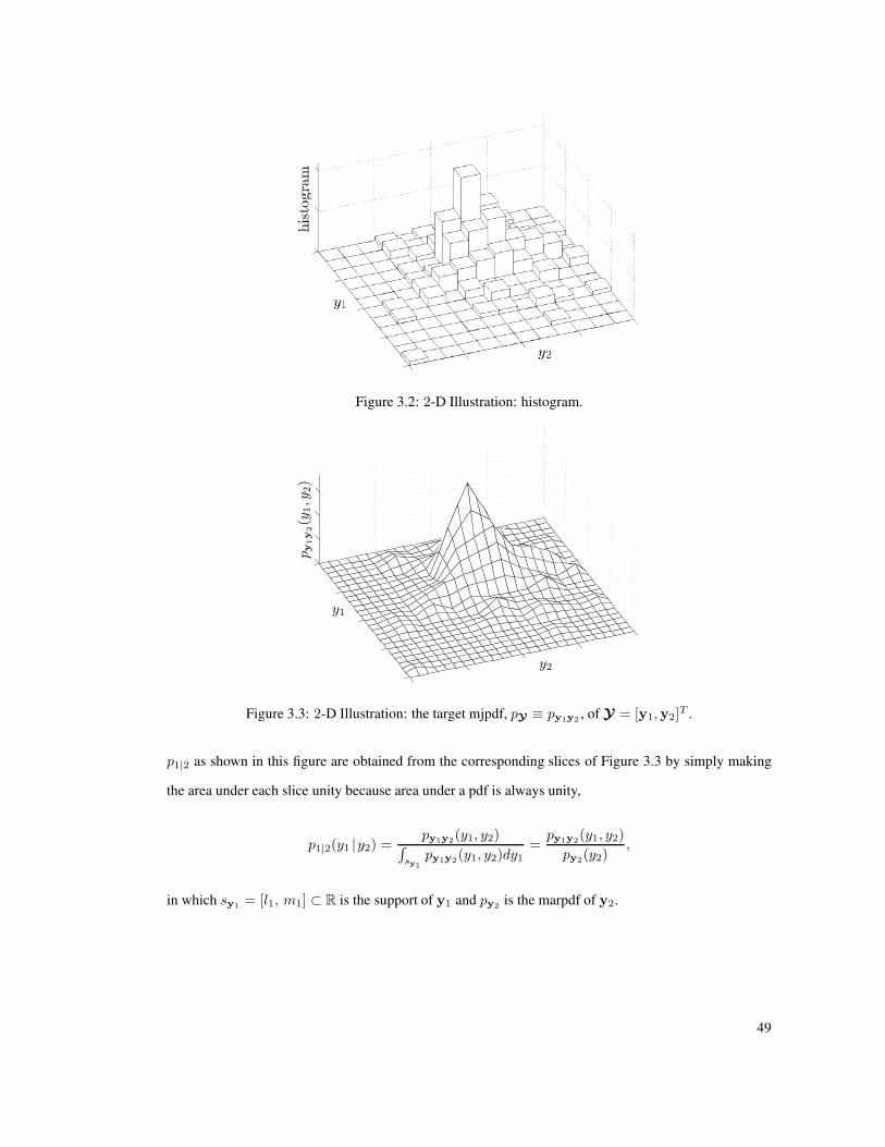
Figure 3.2: 2-D Illustration: histogram.

y1

y2

py

1y

2(y

1,y

2)

Figure 3.3: 2-D Illustration: the target mjpdf, pY ≡ py1y2 , of Y = [y1,y2]T .

p1|2 as shown in this figure are obtained from the corresponding slices of Figure 3.3 by simply making

the area under each slice unity because area under a pdf is always unity,

p1|2(y1 |y2) =py1y2(y1, y2)∫

sy1py1y2(y1, y2)dy1

=py1y2(y1, y2)

py2(y2),

in which sy1 = [l1, m1] ⊂ R is the support of y1 and py2 is the marpdf of y2.

49

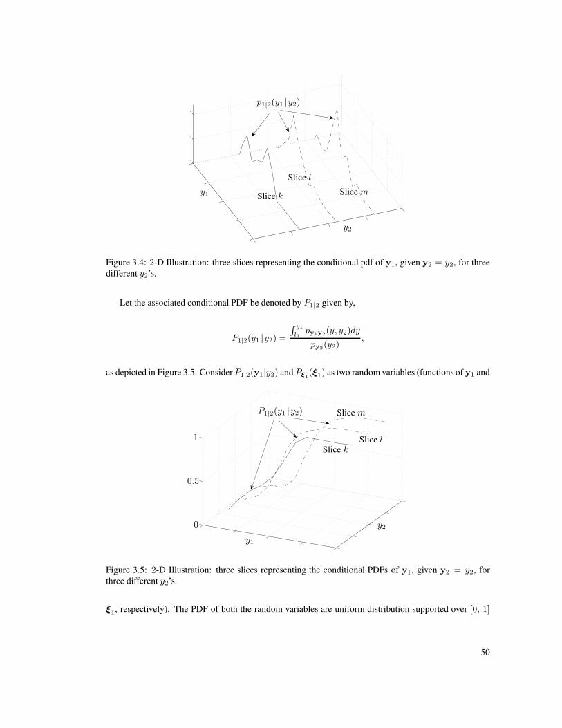
y1

y2

p1|2(y1 |y2)

Slice k

Slice l

Slice m

Figure 3.4: 2-D Illustration: three slices representing the conditional pdf of y1, given y2 = y2, for three

different y2’s.

Let the associated conditional PDF be denoted by P1|2 given by,

P1|2(y1 |y2) =

∫ y1

l1py1y2(y, y2)dy

py2(y2),

as depicted in Figure 3.5. ConsiderP1|2(y1|y2) and Pξ1(ξ1) as two random variables (functions of y1 and

y1

y2

P1|2(y1 |y2)

Slice kSlice l

Slice m

0

0.5

1

Figure 3.5: 2-D Illustration: three slices representing the conditional PDFs of y1, given y2 = y2, for

three different y2’s.

ξ1, respectively). The PDF of both the random variables are uniform distribution supported over [0, 1]

50

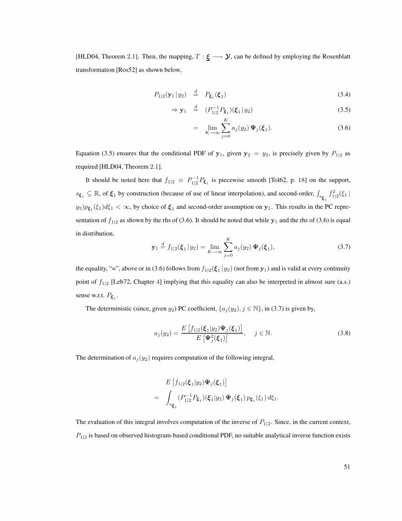
[HLD04, Theorem 2.1]. Then, the mapping, T : ξ −→ Y , can be defined by employing the Rosenblatt

transformation [Ros52] as shown below,

P1|2(y1 |y2) d= Pξ1

(ξ1) (3.4)

⇒ y1d= (P−1

1|2Pξ1)(ξ1 |y2) (3.5)

= limK→∞

K∑

j=0

aj(y2)Ψj(ξ1). (3.6)

Equation (3.5) ensures that the conditional PDF of y1, given y2 = y2, is precisely given by P1|2 as

required [HLD04, Theorem 2.1].

It should be noted here that f1|2 ≡ P−11|2Pξ1

is piecewise smooth [Tol62, p. 18] on the support,

sξ1⊆ R, of ξ1 by construction (because of use of linear interpolation), and second-order,

∫sξ1

f21|2(ξ1 |

y2)pξ1(ξ1)dξ1 < ∞, by choice of ξ1 and second-order assumption on y1. This results in the PC repre-

sentation of f1|2 as shown by the rhs of (3.6). It should be noted that while y1 and the rhs of (3.6) is equal

in distribution,

y1d= f1|2(ξ1 |y2) = lim

K→∞

K∑

j=0

aj(y2)Ψj(ξ1), (3.7)

the equality, “=”, above or in (3.6) follows from f1|2(ξ1 |y2) (not from y1) and is valid at every continuity

point of f1|2 [Leb72, Chapter 4] implying that this equality can also be interpreted in almost sure (a.s.)

sense w.r.t. Pξ1.

The deterministic (since, given y2) PC coefficient, {aj(y2), j ∈ N}, in (3.7) is given by,

aj(y2) =E[f1|2(ξ1|y2)Ψj(ξ1)

]

E[Ψ2

j (ξ1)] , j ∈ N. (3.8)

The determination of aj(y2) requires computation of the following integral,

E[f1|2(ξ1|y2)Ψj(ξ1)

]

=

∫

sξ1

(P−11|2Pξ1

)(ξ1|y2)Ψj(ξ1) pξ1(ξ1) dξ1.

The evaluation of this integral involves computation of the inverse of P1|2. Since, in the current context,

P1|2 is based on observed histogram-based conditional PDF, no suitable analytical inverse function exists

51

for such nonparametric PDF. Therefore, inverse of this function needs to evaluated numerically while

evaluating the above integral. This might be computationally expensive or/and numerically instable. A

computationally efficient scheme based on a surrogate function (instead of using P−11|2Pξ1

) is described in

the Appendix.

For several different values of y2 ∈ sy2 , the PC coefficients, {aj(y2)}j∈N, need to be computed. Let

the support, sy2 = [l2, m2] ⊂ R, be divided equally into n2 ∈ N intervals. Then, coordinates of the

points defining these intervals are given by y(k)2 = l2 + k[(m2 − l2)/n2], k = 0, · · · , n2. For each slice

defined by P1|2(y1 | y(k)2 ), compute the PC coefficients, {aj(y

(k)2 )}j∈N, by using (3.8). A few typical

profiles of the mapping, N ∋ j 7−→ aj(y2) ∈ R, for given y2 are depicted in Figure 3.6.

j ∈N

y2

aj(y(k)2 )

aj(y(l)2 )

aj(y(m)2 )

Slice kSlice l

Slice m

0

0

5

10

15

−0.2

0.2

0.4

Figure 3.6: 2-D Illustration: j 7−→ aj(y2) for given y2.

For any given j ∈ N, the set of pairs, {y(k)2 , aj(y

k2 )}n2

k=0, as just determined is next used to construct

the mapping, sy2 ∋ y2 7−→ aj(y2) ∈ R, by simply employing a linear interpolation scheme (note that this

is an 1-D version of a similar problem for estimating pdf from the histogram defined only over a discrete

array of points as already encountered). A few profiles of this mapping are sketched in Figure 3.7.

Since n2 ∈ N is a finite (but large) number, the mapping, y2 7−→ aj(y2), for any given j ∈ N,

defined via linear interpolation with {y(k)2 , aj(y

k2 )}n2

k=0, is piecewise smooth. By the second-order con-

dition on f1|2, it also implies that | aj(y2) |< ∞ for any given j ∈ N. It is, therefore, straight-

forward to select a suitable weight, say, defined by sy2 ∋ y2 7−→ w2(y2) ∈ (0, ∞), such that

∫sy2

a2j(y2)w2(y2)dy2 <∞. Then, a set of basis functions, {ψk}k∈N, orthogonal w.r.t. the weight w2(·),

52

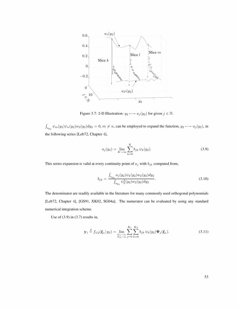
j ∈N

y2

a1(y2)

aP (y2)

Slice k

Slice lSlice m

0

0

10

−0.2

0.2

0.4

0.6

Figure 3.7: 2-D Illustration: y2 7−→ aj(y2) for given j ∈ N.

∫sy2

ψm(y2)ψn(y2)w2(y2)dy2 = 0, m 6= n, can be employed to expand the function, y2 7−→ aj(y2), in

the following series [Leb72, Chapter 4],

aj(y2) = limK→∞

K∑

k=0

bjk ψk(y2). (3.9)

This series expansion is valid at every continuity point of aj with bjk computed from,

bjk =

∫sy2

aj(y2)ψk(y2)w2(y2)dy2∫

sy2ψ2

k(y2)w2(y2)dy2. (3.10)

The denominator are readily available in the literature for many commonly used orthogonal polynomials

[Leb72, Chapter 4], [GS91, XK02, SG04a]. The numerator can be evaluated by using any standard

numerical integration scheme.

Use of (3.9) in (3.7) results in,

y1d= f1|2(ξ1 |y2) = lim

K1→∞

K2→∞

K1∑

j=0

K2∑

k=0

bjk ψk(y2)Ψj(ξ1). (3.11)

53

Now, the marPDF, P2, of y2 can be similarly (consider 1-D cases of the series of Figures 3.1-3.6)

employed to obtain the following PC expansion for y2,

y2d= f2(ξ2) = lim

K→∞

K∑

j=0

cj Ψj(ξ2), (3.12)

in which f2 ≡ P−12 Pξ2

and cj is given by,

cj =E [f2(ξ2)Ψj(ξ2)]

E[Ψ2

j (ξ2)] , j ∈ N, (3.13)

and can be efficiently computed by using the simple scheme described in the Appendix.

The PC expansions, (3.11) and (3.12), constructed from the available measurement data, together

completely characterize the random vector, Y = [y1,y2]T . In a computational set-up, the series in (3.11)

and (3.12) are truncated after suitable large number of terms.

Sampling of Y is straightforward. The random variables, ξ1 and ξ2, are statistically independent.

First, use (3.12) to generate a sample, y2, of y2 and then use the realized value, y2, in (3.11) to get y1.

Repeat the process until the desired number of samples of Y = [y1,y2]T is generated.

Extension of the above 2-D formulation to the N -variate Y is now summarized below,

y1d= P−1

1|2:NPξ1(ξ1 |y2, · · · , yN)

=

K(1)1∑

i1=0

· · ·K

(1)N∑

iN =0

b(1)i1i2···iN

ψiN (yN) · · ·ψi2(y2)Ψi1(ξ1)

y2d= P−1

2|3:NPξ2(ξ2 |y3, · · · , yN)

=

K(2)2∑

i2=0

· · ·K

(2)N∑

iN =0

b(2)i2···iN

ψiN (yN) · · ·ψi3 (y3)Ψi2(ξ2)

...

yN

d= P−1

NPξN

(ξN) =

K(N)N∑

iN =0

b(N)

iNΨiN (ξ

N).

Here, Pi|(i+1):N is conditional PDF of yi, given yi+1 = yi+1, · · · ,yN = yN , induced by PY and

b(i)jiji+1···jN

represents (N − (i − 1))-dimensional matrix of PC coefficients of size K(i)i × · · · × K

(i)N

with K(i)i , · · · ,K(i)

N being the suitable large integers retained in the corresponding series expansion. The

54

random variables, ξ1, · · · , ξN , are statistically independent. Each digital sample of Y is generated starting

with sampling yN and successively proceeding towards sampling yN−1,yN−2, · · · , and in last sampling

y1.

Finally, let us conclude this section by emphasizing that Pi|(i+1):N should not be computed by inte-

grating pY since it would then involve a substantial computational effort to perform several multidi-

mensional integrations while approximating the corresponding function, P−1i|(i+1):NPξi

(see Appendix).

Instead, Pi|(i+1):N should be computed from estimate of mjpdf of (yi, · · · ,yN) determined by consider-

ing only the measurement data associated with yi, · · · ,yN , and completely ignoring the data associated

with y1, · · ·yi−1. This would always involve 1-D integration in computation of Pi|(i+1):N ,

Pi|(i+1):N(yi |yi+1, · · · , yN) =

∫ yi

lipyi,··· ,yN (yi, · · · , yN) dyi

pyi+1,··· ,yN (yi+1, · · · , yN).

Here, the integration is carried over the domain, [li, yi] ⊆ syi = [li, mi] ⊂ R, where syi is the support of

yi. This scheme would be relatively computationally inexpensive even after the additional computational

overhead required to estimate the set of pdfs, py2,··· ,yN , py3,··· ,yN , · · · , pyN , (from the corresponding

data) that need to determined only once at the outset.

3.2.2 Approach 2: Based on Marginal PDFs and SRCC

In this approach, the unknown relationship between ξ and Y is defined again by having recourse to the

Rosenblatt transformation establishing a set of N mappings, each of which is similar to (3.12), between

the corresponding k-th components, yk and ξk, k = 1, · · · , N . It should be noted that the Rosenblatt

transformation, when applied on marPDF of a scalar-variate random variable, is similar to the Nataf

transformation. Only marPDF of yk is used in this approach. Unlike ξk’s in Approach 1, the random

variables, ξ1, · · · , ξN, here are, however, statistically dependent enforcing the required statistical depen-

dencies among yk’s. The statistical dependency is characterized via SRCC. In the following, the definition

and the relevant properties of SRCC are briefly reviewed first before describing Approach 2.

Spearman’s Rank Correlation Coefficient

The rank correlation coefficient or Spearman’s rho is named after Charles Edward Spearman who first

introduced it [Spe04]. The rank correlation coefficient between random variables, yi and yj , is simply

55

the PCC applied to the rank of the observed samples of yi and yj rather than to their observed or measured

values. When there is no tie in the observed values of the data, a simple formula exists for the calculation

of SRCC [Man01, p. 655]. Further theoretical treatment and calculation procedural of SRCC including

the case of tied data values can be found in the literature (see e.g., [Leh75, p. 297-303], [PTVF96, p. 634-

637]). Statistical toolbox of MATLAB provides function, corr, that can be used to calculate SRCC.

Definition 3.2.1 The Spearman’s rank correlation coefficient between two random variables, yi and

yj , with marginal probability distribution functions, respectively, being given by Pyi and Pyj , is defined

as,

ρs(yi,yj) = ρ(Pyi(yi), Pyj (yj)) = 12 cov(Pyi(yi), Pyj (yj)). (3.14)

Here, ρ is the Pearson’s correlation coefficient (or the usual product-moment correlation coefficient), cov

is the covariance and the multiplying factor, 12, emanates from variance of Pyk(yk), k = i, j, since

Pyk(yk) ∼ U(0, 1) with U(0, 1) being uniform distribution on [0, 1] (see, e.g.,[HLD04, Theorem 2.1]).

It must be noted from the above definition that SRCC and PCC coincide if PDFs of yi and yj are

U(0, 1). In general, they are, however, different.

A collection of a few salient properties of ρs is enlisted below [EMS01, Section 4.3], [KC06, Sec-

tion 3.2.2]. It

• always exists and is symmetric;

• is independent of marpdf of yi and yj ;

• is invariant under strictly monotone transformation of yi and yj ;

• can take any values from the closed interval, [−1, 1];

• is zero if yi and yj are statistically independent, the converse is not true.

The most important property to be used in the present work is invariance under monotone transformation

property of SRCC.

56

Now that the relevant information on SRCC is set forth, Approach 2 is described below by introducing

the mapping, ξk 7−→ yk, k = 1, · · · , N , through the use of the Rosenblatt transformation [Ros52] applied

on each ξk separately,

ykd= qk(ξk) = lim

Kk→∞

Kk∑

j=0

cjk Ψj(ξk), qk(ξk) ≡ P−1ykPξk

. (3.15)

This PC representation is similar to (3.12). The marPDF, Pyk, is estimated from the normalized and

linearly interpolated 1-D histogram of the measurement data on each random variable component, yk,

separately. This can be readily performed as already discussed in section 3.2.1. The PC representation

of qk in (3.15) is, therefore, valid at every continuity of qk implying that the equality, ‘=’, can also be

interpreted in a.s. sense w.r.t. Pξk. The PC coefficient, cjk, is given by,

cjk =E [qk(ξk)Ψj(ξk)]

E[Ψ2

j(ξk)] , j ∈ N. (3.16)

A simple and computationally efficient scheme based on 1-D interpolated surrogate function, approxi-

mating P−1ykPξk

, is described in Appendix to determine {cjk}j∈N, k = 1, · · · , N .

The series in (3.15) is truncated after a large number of terms, Kk. Since SRCC is preserved under

monotone transformation, the SRCC matrices of ξ = [ξ1, · · · , ξN ]T and Y are identical. The target

N × N SRCC matrix, [ρs], is simply estimated from the available measurement data on Y . If (i, j)-

th, i, j = 1, · · · , N , element of [ρs] is denoted by (ρs)ij , then (ρs)ij = ρs(yi,yj). The samples of

ξ, with SRCC matrix, [ρs], are first generated. Subsequently, samples of each ξk are substituted in the

corresponding PC expansion of yk to obtain the realizations of yk . The resulting samples of Y are

consistent with the target set, {pyk}N

k=1, of marpdfs and the target SRCC matrix, [ρs].

The commonly used PC random variables, ξ1, · · · , ξN , that are often chosen to construct PC rep-

resentation, are standard Gaussian random variables, uniform random variables on [−1, 1], beta type I

random variables on [−1, 1] or gamma random variables. The generation of samples of such statistically

independent random variables, as required in Approach 1, is straightforward. The samples of statistically

dependent random variables, particularly when the statistical dependency is characterized by a specified

SRCC matrix, [ρs], as required in Approach 2, can also be readily generated by using the existing sim-

ulation techniques. However, these simulation schemes are scattered across the spectrum of literatures:

57

MC simulation to management science. Therefore, for the sake of completeness of the present work,

two useful and easily implementable techniques are summarized in the next two subsections. These two

techniques are directly related to concept of copula [Joe97, EMS01, Nel06, KC06] knowledge of which,

though useful, is not required here.

Normal Copula Technique

This technique assumes existence of an underlying correlated N -D standard Gaussian random vector,

X = [x1, · · · ,xN ]T , in which each component, xi, is a standard Gaussian random variable. If X exists,

i.e., if a feasible (positive-definite) covariance matrix is found, then it is the fastest method among all

the currently existing methods. In such situation, the correlation (also, covariance) matrix, [ρ], of X is

determined as follows.

It was shown by Pearson in 1904 that [KC06, p. 51 and p. 75-77],

ρ(xi,xj) = 2 sin(π

6ρs(ui,uj)

), (3.17)

in which ui ∼ U(0, 1) and uj ∼ U(0, 1) are uniform random variables. If PDF of the standard Gaussian

random variable is denoted by Φ(·), then Φ(xi) ∼ U(0, 1), ∀i [HLD04, Theorem 2.1]. Let us then

select ui’s in (3.17) as ui ≡ Φ(xi). Consider now the following mapping based on the Rosenblatt

transformation,

ui ≡ Φ(xi)d= Pyi(yi), i = 1, · · · , N, (3.18)

sincePyi(yi) ∼ U(0, 1) [HLD04, Theorem 2.1]. By the invariance under monotone transformation prop-

erty of the SRCC, we have ρs(yi,yj) = ρs(Pyi(yi), Pyj (yj)). Then, by (3.14) and “d=” in (3.18), the

SRCC matrix of U = [u1, · · · ,uN ]T is given by [ρs] with its (i, j)-th element being given by ρs(yi,yj)

estimated based on the measurement data on Y . The correlation (or covariance) matrix, [ρ], of X then

follows from (3.17), with the (i, j)-th, i, j = 1, · · · , N , element, ρij , of [ρ] being given by ρ(xi,xj). Sim-

ulation of the standard Gaussian random vector, X, with covariance matrix, [ρ], is then straightforward.

In the literature, PDF of U is usually referred as normal copula.

58

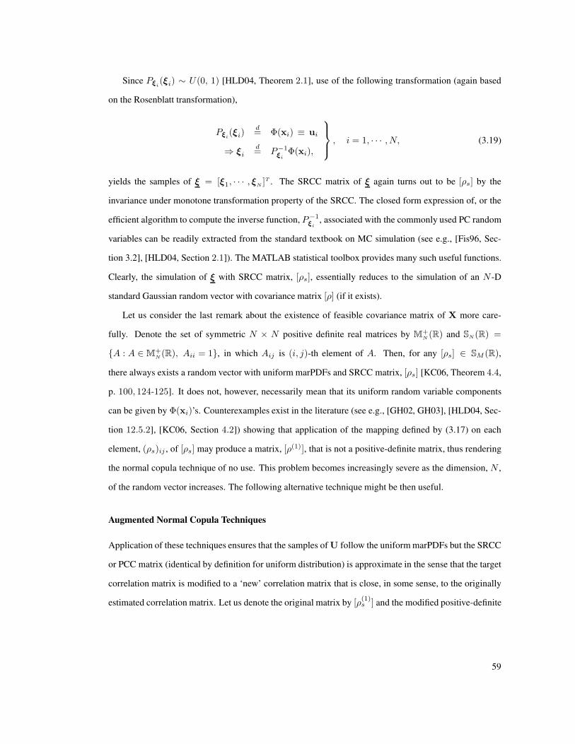
Since Pξi(ξi) ∼ U(0, 1) [HLD04, Theorem 2.1], use of the following transformation (again based

on the Rosenblatt transformation),

Pξi(ξi)

d= Φ(xi) ≡ ui

⇒ ξid= P−1

ξiΦ(xi),

, i = 1, · · · , N, (3.19)

yields the samples of ξ = [ξ1, · · · , ξN ]T . The SRCC matrix of ξ again turns out to be [ρs] by the

invariance under monotone transformation property of the SRCC. The closed form expression of, or the

efficient algorithm to compute the inverse function, P−1ξi

, associated with the commonly used PC random

variables can be readily extracted from the standard textbook on MC simulation (see e.g., [Fis96, Sec-

tion 3.2], [HLD04, Section 2.1]). The MATLAB statistical toolbox provides many such useful functions.

Clearly, the simulation of ξ with SRCC matrix, [ρs], essentially reduces to the simulation of an N -D

standard Gaussian random vector with covariance matrix [ρ] (if it exists).

Let us consider the last remark about the existence of feasible covariance matrix of X more care-

fully. Denote the set of symmetric N × N positive definite real matrices by M+N (R) and SN(R) =

{A : A ∈ M+N(R), Aii = 1}, in which Aij is (i, j)-th element of A. Then, for any [ρs] ∈ SM (R),

there always exists a random vector with uniform marPDFs and SRCC matrix, [ρs] [KC06, Theorem 4.4,

p. 100, 124-125]. It does not, however, necessarily mean that its uniform random variable components

can be given by Φ(xi)’s. Counterexamples exist in the literature (see e.g., [GH02, GH03], [HLD04, Sec-

tion 12.5.2], [KC06, Section 4.2]) showing that application of the mapping defined by (3.17) on each

element, (ρs)ij , of [ρs] may produce a matrix, [ρ(1)], that is not a positive-definite matrix, thus rendering

the normal copula technique of no use. This problem becomes increasingly severe as the dimension, N ,

of the random vector increases. The following alternative technique might be then useful.

Augmented Normal Copula Techniques

Application of these techniques ensures that the samples of U follow the uniform marPDFs but the SRCC

or PCC matrix (identical by definition for uniform distribution) is approximate in the sense that the target

correlation matrix is modified to a ‘new’ correlation matrix that is close, in some sense, to the originally

estimated correlation matrix. Let us denote the original matrix by [ρ(1)s ] and the modified positive-definite

59

correlation matrix by [ρs]. With this new target correlation matrix, [ρs], the use of the normal copula

technique, as described in the previous subsection, becomes feasible.

One such technique [vdG98, Section 5] suggests to adapt [ρ(1)s ] and [ρ(1)], to new positive-definite

correlation matrices, [ρs] and [ρ], by using a simple iterative scheme based on the spectral decomposition

of real Hermitian matrices. While this scheme might work in practice, it is likely to be little unwieldy, par-

ticularly in high dimension, requiring too many iterations often resulting in relatively large error between

the old and modified matrices.

Another technique [GH03] is a constrained minimization problem in the space of X and relatively

more robust. Two metrics, in particular, L1 =∑

i<j |ρij − ρ(1)ij | norm and L∞ = maxi<j |ρij − ρ

(1)ij |

norm, are minimized subject to [ρ] ∈ SN(R) [GH03]. It is, however, not guaranteed that the resulting

‘new’ correlation matrix, [ρs], of U (by applying the inverse transformation of (3.17) on [ρ]) would

be positive-definite and close to the originally specified target correlation matrix, [ρ(1)s ], of U. In such

situation, an iterative scheme like the one proposed earlier in the literature [vdG98, Section 5] might be

adopted.

In the present work, the following constrained minimization problem, similar to the works presented

in the literature [GH03], is recommended,

minimize ‖[ρ] − [ρ(1)]‖F

subject to [ρ] ∈ SN(R),(3.20)

or/and other meaningful constraints (see e.g., [GH03, Section 5]). The Frobenius norm is preferred (over

L1 and L∞ norms) since it shows relatively much smaller error (even in high dimension). The above

optimization problem can be efficiently solved by employing the semi-definite program (SDP) [VB96],

[Dat05, Chapter 4]. Many efficient freely available softwares1 exist to solve such SDP. In the present

work, a public domain MATLAB toolbox, YALMIP, developed by Lofberg ([Lof04]), is used.

The techniques as discussed above should be applied only if the new correlation matrix, [ρs], of U is

positive-definite and is close, in the appropriate sense, to the originally specified target correlation matrix,

[ρ(1)s ]. Otherwise, alternative techniques [MB93, MB97, GH02, KC06] at the expense of significantly

additional computational time and resource might be interrogated. In many practical applications, the two

1http://www-user.tu-chemnitz.de/˜helmberg/semidef.html

60

recommended techniques — normal copula technique and augmented normal copula technique — are,

nevertheless, likely to be satisfactory.

3.3 Practical Illustration and Discussion

The proposed techniques are employed here to construct the PC representation of a spatio-temporal ran-

dom temperature field by using a set of oceanographic data obtained from a shallow-water acoustics

transmission experiment. This experiment would be referred now onwards as SWARM95 (Shallow Water

Acoustics in Random Medium) experiment. It was conducted during the month of July-August in 1995

in the Mid-Atlantic Bight continental shelf region off the coast of New Jersey [ABC+97].

The primary objective of the SWARM95 experiment is to investigate the effects of random varia-

tions of the oceanographic parameters, for example, temperature and salinity fields, on the statistical

properties of the acoustic field. The acoustic field is perturbed significantly by a small change in water

column sound speed distribution. The sound speed variation depends on the internal wave field and the

oceanographic parameters through an integral equation. This internal wave field is also governed by par-

tial differential equations with random coefficients depending on the oceanographic parameters. Further

details and precise objective of the experiment are documented and discussed in other research papers

[ABC+97, FOT+00]. In the current chapter, modeling of the spatio-temporal random temperature field

from the oceanographic measurements of SWARM95 experiment would only be considered. The PC rep-

resentation of the spatio-temporal random field modeling the oceanographic parameters would be useful

in propagating the uncertainty in a rational manner to the prediction of the acoustic field and in estimat-

ing the confidence interval of the associated statistical parameters by employing the techniques available

elsewhere [GRH99, PG04, DG04, GD06, DGS08] (also see chapter 2).

There are 3 vertical strings through 72 m depth of water column each with 11 temperature sen-

sors measuring the temperature histories. These temperature senors are located at depth h ∈ D =

{16, 21, 26, 31, 36, 38.5, 41, 46, 48.5, 51, 56} m. The temperature data are sampled every minute and

there is a total of 17281 samples from each sensor. The three strings would hereafter be referred as tav309,

tav307 and tav598 as per nomenclature rule decided earlier for a different analysis (not a part of the cur-

rent work) conducted on this set of temperature data. A few typical time histories obtained from tav309

are shown in Figure 3.8. However, it is imperative to separate the background internal wave field from the

61

time (min)

tem

per

atu

re(◦

C)

quiescent zone(99 samples @ 1 min rate)

depth 16 mdepth 36 mdepth 48.5 m

0 500 1000 1500

10

15

20

25

Figure 3.8: A few experimentally measured time histories (shown only for a segment of the total experi-

mental time span).

solitary wave contribution while computing some intermediate oceanographic parameters, for example,

buoyancy frequency, that is required to compute the sound speed fluctuation [FOT+00]. Therefore, only

the “quiescent” part of the measurement data excluding the solitary waves must be used while comput-

ing such intermediate parameters. The most active solitary wave region is in the upper half of the water

column.

3.3.1 Selecting the Regions of Low Internal Solitary Wave Activity

There is some subjectivity in choosing the quiescent part of the temperature data because it is next to

impossible to completely separate the background internal wave field from the solitary wave contribution.

The mathematical decomposition of the sound speed distribution into deterministic, time-dependent field

and a random fluctuation about this deterministic field, as discussed in previous work [FOT+00], is an

idealization. In a real ocean experiment, the situation is much more complicated. In order to estimate

the oceanographic parameters, e.g., buoyancy frequency, it is important to try to stay away from regions

containing the obvious large fluctuations that often start with a jump discontinuity. These regions are

usually associated with the main components of the solitary wave train. Therefore, the highly variable

regions, containing the strong solitary wave activity, are not used in the following analysis.

By visual inspection, the regions in the boxes, for example, as shown in Figure 3.8, are examples of

“low” internal solitary wave activity and suitable for reliable estimation of the buoyancy frequency, and

62

consequently, selected for further analysis. A total of such 8 time-segments each with 99 temperature

measurements at any h ∈ D are selected from the whole span of the experimentally measured time

history. Out of 17281 samples available from each sensor, only 8 × 99 samples are deemed to be useful

in constructing the PC representation of the spatio-temporal random temperature field. The resulting PC

representation would be useful for other analysis involving (stochastic) oceanographic parameters that

depend on the random temperature field.

More detailed features of a typical quiescent segment showing the time histories collected from a

few sensors (at different depths) attached to one of the 3 strings (tav309) are shown in Figure 3.9. Each

time (min)

tem

per

atu

re(◦

C)

depth 16 mdepth 36 mdepth 48.5 m

11 samples @ 1 min rate

840 860 880 900 920 938

10

15

20

25

Figure 3.9: A typical quiescent zone divided into 9 smaller segments with 11 samples (shown for a few

sensors).

quiescent segment with 99 samples is further divided into 9 smaller segments with each containing 11

samples as shown in this figure.

At any given time instant, all the 11 sensors located at h ∈ D are measuring the temperature (at 1 min

sampling rate) simultaneously. Consider a spatio-temporal domain defined by one smaller segment asso-

ciated with the quiescent zone and the 72 m depth of water column along which SWARM95 experiment

was conducted. Let us assume that the random temperature field is statistically independent and identi-

cally distributed (i.i.d.) both across the smaller segments with 11 samples as shown in Figure 3.9 within a

given quiescent zone as well as across the different quiescent zones as shown in Figure 3.8. Without any

further loss of generality, time can be, therefore, conveniently reset to t = 0 at the beginning of each of

these smaller segments as illustrated in Figure 3.10. Denote the spatio-temporal domain thus described by

63

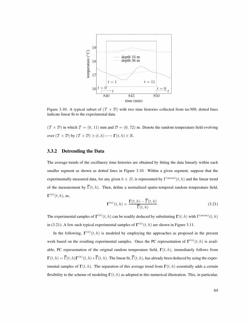
time (min)

tem

per

atu

re(◦

C)

depth 16 mdepth 36 m

t = 1 t = 11

t = 0 t = 0tt

840 845 850

16

17

18

19

Figure 3.10: A typical subset of (T × D) with two time histories collected from tav309; dotted lines

indicate linear fit to the experimental data.

(T × D) in which T = (0, 11) min and D = (0, 72) m. Denote the random temperature field evolving

over (T × D) by (T × D) ∋ (t, h) 7−→ Γ(t, h) ∈ R.

3.3.2 Detrending the Data

The average trends of the oscillatory time histories are obtained by fitting the data linearly within each

smaller segment as shown as dotted lines in Figure 3.10. Within a given segment, suppose that the

experimentally measured data, for any given h ∈ D, is represented by Γ(meas)(t, h) and the linear trend

of the measurement by Γ(t, h). Then, define a normalized spatio-temporal random temperature field,

Γ(n)(t, h), as,

Γ(n)(t, h) =Γ(t, h) − Γ(t, h)

Γ(t, h). (3.21)

The experimental samples of Γ(n)(t, h) can be readily deduced by substituting Γ(t, h) with Γ(meas)(t, h)

in (3.21). A few such typical experimental samples of Γ(n)(t, h) are shown in Figure 3.11.

In the following, Γ(n)(t, h) is modeled by employing the approaches as proposed in the present

work based on the resulting experimental samples. Once the PC representation of Γ(n)(t, h) is avail-

able, PC representation of the original random temperature field, Γ(t, h), immediately follows from

Γ(t, h) = Γ(t, h)Γ(n)(t, h)+Γ(t, h). The linear fit, Γ(t, h), has already been deduced by using the exper-

imental samples of Γ(t, h). The separation of this average trend from Γ(t, h) essentially adds a certain

flexibility to the scheme of modeling Γ(t, h) as adopted in this numerical illustration. This, in particular,

64

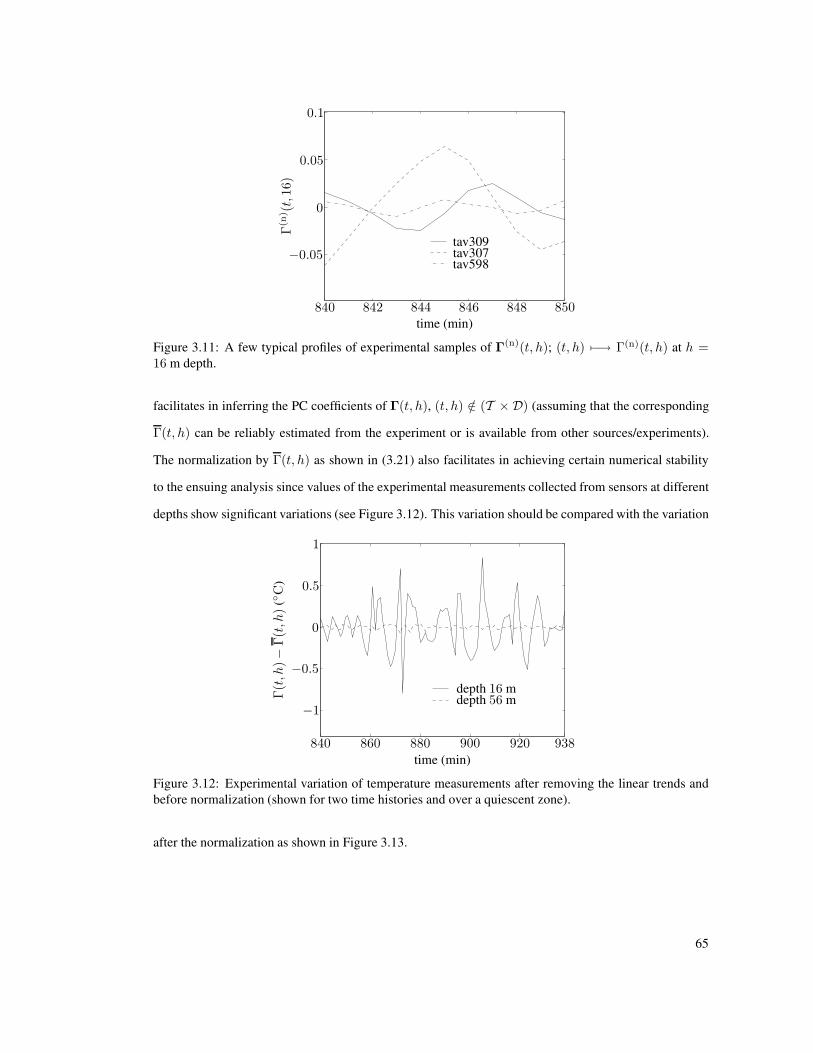
time (min)

Γ(n

) (t,

16)

tav309tav307tav598

840 842 844 846 848 850

−0.05

0

0.05

0.1

Figure 3.11: A few typical profiles of experimental samples of Γ(n)(t, h); (t, h) 7−→ Γ(n)(t, h) at h =16 m depth.

facilitates in inferring the PC coefficients of Γ(t, h), (t, h) /∈ (T × D) (assuming that the corresponding

Γ(t, h) can be reliably estimated from the experiment or is available from other sources/experiments).

The normalization by Γ(t, h) as shown in (3.21) also facilitates in achieving certain numerical stability

to the ensuing analysis since values of the experimental measurements collected from sensors at different

depths show significant variations (see Figure 3.12). This variation should be compared with the variation

time (min)

Γ(t,h

)−

Γ(t,h

)(◦

C)

depth 16 mdepth 56 m

840 860 880 900 920 938

−1

−0.5

0

0.5

1

Figure 3.12: Experimental variation of temperature measurements after removing the linear trends and

before normalization (shown for two time histories and over a quiescent zone).

after the normalization as shown in Figure 3.13.

65

time (min)

Γ(n

)(t,h

)

depth 16 mdepth 56 m

840 860 880 900 920 938

−0.06

−0.04

−0.02

0

0.02

0.04

0.06

Figure 3.13: Variation of the normalized temperature measurements (shown for two time histories and

over a quiescent zone).

3.3.3 Stochastic Modeling of Γ(n)(t, h)

For any given (t, h) ∈ (T × D), Γ(n)(t, h) represent a random variable. Clearly, the experimental

measurements essentially represent the samples of a finite set of these random variables. Recall that D

represents the set of coordinates of the sensors attached to the strings along 72 m water column. Let us

now also denote the set of time instants (per convention of Figure 3.10) of collection of experimental

samples by T = {1, 2, · · · , 10, 11} (since sampling rate is 1 min). Note the difference between the

continuous space, (T ×D), over which Γ(n)(t, h) is evolving and the discrete space, (T ×D), consisting

of only a finite set of points at which the experimental samples are available.

Let us denote the set of 11 × 11 random variables, {Γ(n)(t, h)}(t,h)∈(T×D), collectively by Y , i.e.,

N = dim(Y) = 121. Since each quiescent zone is divided into 9 smaller segments (see Figure 3.9)

and 8 quiescent zones are selected (see section 3.3.1) across the whole span of the experimental time

histories, there are 8 × 9 = 72 statistically independent samples of Y from each string. In the present

work, a space and time separability condition of statistical dependency of the original random temperature

field is assumed for the time and spatial extent spanning the sea surface. However, no such space-time

separability is assumed for the time and depth, i.e., for (T × D). The random variable components of

Y are, therefore, statistically dependent. From three vertical strings, tav309, tav307 and tav598 (about

10 km away from each other), a total of n = 3 × 72 = 216 samples of Y are available.

The task is now to construct PC representations of Y by using the approaches as proposed in the

present work with 210 samples of Y . The PC representations would be consistent with the information

66

extracted from these 210 experimental samples. Further details and results are discussed in the next

subsections.

3.3.4 Modeling of Y via Approach 1

The Karhunen-Loeve (KL) decomposition is first employed to construct a reduced order model of the

non-Gaussian random vector, Y . Though the resulting non-Gaussian KL random variable components are

uncorrelated, they are, in general, statistically dependent. Approach 1 is subsequently used to characterize

this reduced order model of Y .

KL Decomposition of Y

Let n experimental samples of Y be denoted by Y1, · · · ,Yn. An estimate ofN ×N covariance matrix of

Y is computed by using the samples as Cyy = (1/(n− 1))YoYTo . Here, Yo = [Y1o, · · · ,Yno] represents

an N × n matrix and Yko ≡ Yk − Y , k = 1, · · · , n, with Y being unbiased estimate of the mean vector

of Y , i.e., Y = (1/n)∑n

k=1 Yk . Following the KL expansion procedure [Loe78, Chapter XI], [Jol02],

let us collect the dominant KL random variable components, {z′1, · · · , z′M}, M < N , in an M -D random

vector, Z ′ = [z′1, · · · , z′M ]T . Here, Z′ is related to Y by (2.2).

The set of experimental samples of Z′ can be immediately obtained by replacing Y with Y1, · · · ,Yn

in (2.2) resulting in Z ′1, · · · ,Z ′

n. To enhance the regularity of the ensuing numerical problem and to

improve the efficiency of the associated computation, this data set is further scaled to obtain another data

set as shown below,

Zk = 2

[(Z ′

k − a)◦(

1

b− a

)]− 1M , k = 1, · · · , n. (3.22)

Here, 1M is an M -D column vector of 1’s, a = [α1, · · · , αM ]T and b = [β1, · · · , βM ]T with αi =

min(z′(1)i , · · · , z′(n)

i ) and βi = max(z′(1)i , · · · , z′(n)

i ), in which z′(k)i is the i-th component of the k-th

sample, Z ′k = [z

′(k)1 , · · · , z′(k)

M ]. Denote this M -D normalized KL random vector associated with the

samples, {Zk}nk=1, by Z = [z1, · · · , zM ]T . The scaling in (3.22) is particularly chosen so that Z is

supported on [−1, 1]M , which would be in concordance, in some sense, of the support, [−1, 1], of the

67

uniform distributions used as measures of the PC random variables in section 3.3.4. The following relation

between Z and Y then holds,

Y ≈ Y(M) = V

[a+

{(b− a)◦

1

2(Z + 1M)

}]+ Y. (3.23)

The approximation sign, ‘≈’, in (3.23) emphasizes that Y is projected into the space spanned only by the

largest M dominant eigenvectors of Cyy to obtain the reduced order representation, Z .

Based on n = 216 samples, the sample covariance matrix,Cyy , is first determined. Here,M is chosen

such that∑

M

i=1 ςi = 0.999∑

N

i=1 var(yi) dictating that M = 78 dominant KL random variables should

be considered (recall that N = dim(Y) = 121). Use of the dominant M eigenvectors, along with the

samples of Y , in (2.2) yields the set of samples of Z′ which, in turn, yields the samples of Z through

(3.22). At this stage, a crosscheck is performed to ensure that enough information is propagated from

Y to Z as the dimension is reduced from N = 121 to M = 78. The samples of Y are reconstructed

back from the samples, {Zk}nk=1, by using (3.23), i.e., Y(recons)

k = V[a+

{(b − a)◦ 1

2 (Zk + 1M)}]

+Y .

The MSE of the relevant statistics computed from {Y(recons)k }n

k=1 are compared with the corresponding

statistics computed from the original experimental samples, {Yk}nk=1. The results are shown in Table 3.1.

Relative MSE in percentage (%) for

Mean Covariance SRCC

vector matrix matrix

0 0 0.1220

Table 3.1: Comparison of statistics based on {Y(recons)k }n

k=1 and {Yk}nk=1: Relative MSE as shown below

is computed as relMSE(S(recons),S) = 100(‖S(recons) − S‖2

F

)/‖S‖2

F, in which S represents sample

statistic of the experimental samples, {Yk}nk=1, i.e., S represents either Y or Cyy or [ρs] as appropriate,

and S(recons) represents the corresponding sample statistic of the reconstructed samples, {Y(recons)k }n

k=1.

Approach 1 as proposed in section 3.2.1 is now employed to construct the PC representation of Z

based on n = 216 experimental samples of Z.

68

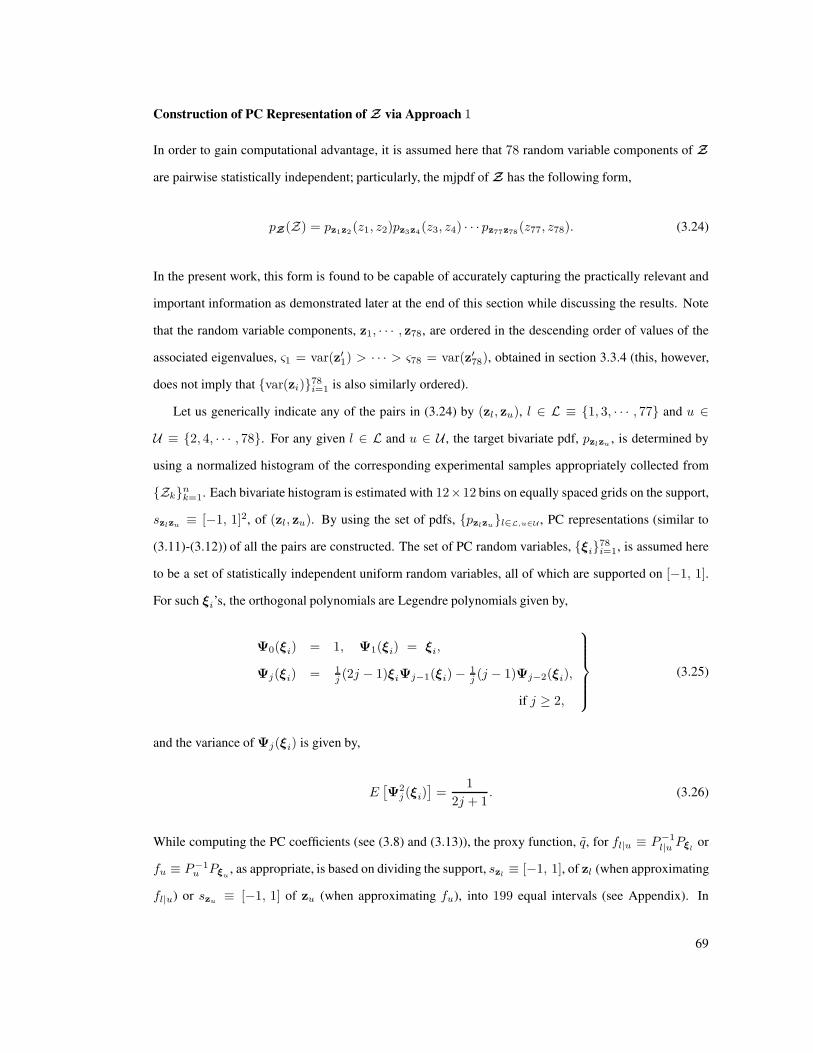
Construction of PC Representation of Z via Approach 1

In order to gain computational advantage, it is assumed here that 78 random variable components of Z

are pairwise statistically independent; particularly, the mjpdf of Z has the following form,

pZ(Z) = pz1z2(z1, z2)pz3z4(z3, z4) · · · pz77z78(z77, z78). (3.24)

In the present work, this form is found to be capable of accurately capturing the practically relevant and

important information as demonstrated later at the end of this section while discussing the results. Note

that the random variable components, z1, · · · , z78, are ordered in the descending order of values of the

associated eigenvalues, ς1 = var(z′1) > · · · > ς78 = var(z′78), obtained in section 3.3.4 (this, however,

does not imply that {var(zi)}78i=1 is also similarly ordered).

Let us generically indicate any of the pairs in (3.24) by (zl, zu), l ∈ L ≡ {1, 3, · · · , 77} and u ∈

U ≡ {2, 4, · · · , 78}. For any given l ∈ L and u ∈ U , the target bivariate pdf, pzlzu , is determined by

using a normalized histogram of the corresponding experimental samples appropriately collected from

{Zk}nk=1. Each bivariate histogram is estimated with 12×12 bins on equally spaced grids on the support,

szlzu ≡ [−1, 1]2, of (zl, zu). By using the set of pdfs, {pzlzu}l∈L,u∈U , PC representations (similar to

(3.11)-(3.12)) of all the pairs are constructed. The set of PC random variables, {ξi}78i=1, is assumed here

to be a set of statistically independent uniform random variables, all of which are supported on [−1, 1].

For such ξi’s, the orthogonal polynomials are Legendre polynomials given by,

Ψ0(ξi) = 1, Ψ1(ξi) = ξi,

Ψj(ξi) = 1j (2j − 1)ξiΨj−1(ξi) − 1

j (j − 1)Ψj−2(ξi),

if j ≥ 2,

(3.25)

and the variance of Ψj(ξi) is given by,

E[Ψ2

j (ξi)]

=1

2j + 1. (3.26)

While computing the PC coefficients (see (3.8) and (3.13)), the proxy function, q, for fl|u ≡ P−1l|u Pξl

or

fu ≡ P−1u Pξu

, as appropriate, is based on dividing the support, szl≡ [−1, 1], of zl (when approximating

fl|u) or szu ≡ [−1, 1] of zu (when approximating fu), into 199 equal intervals (see Appendix). In

69

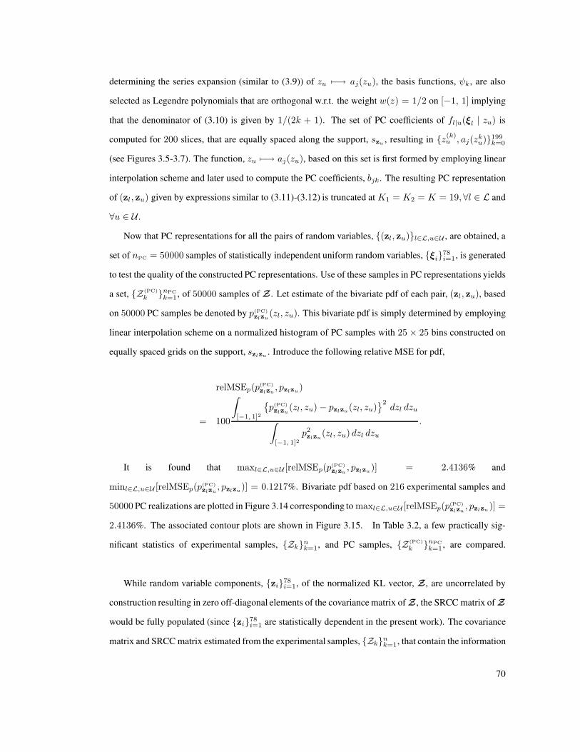
determining the series expansion (similar to (3.9)) of zu 7−→ aj(zu), the basis functions, ψk, are also

selected as Legendre polynomials that are orthogonal w.r.t. the weight w(z) = 1/2 on [−1, 1] implying

that the denominator of (3.10) is given by 1/(2k + 1). The set of PC coefficients of fl|u(ξl | zu) is

computed for 200 slices, that are equally spaced along the support, szu , resulting in {z(k)u , aj(z

ku)}199

k=0

(see Figures 3.5-3.7). The function, zu 7−→ aj(zu), based on this set is first formed by employing linear

interpolation scheme and later used to compute the PC coefficients, bjk. The resulting PC representation

of (zl, zu) given by expressions similar to (3.11)-(3.12) is truncated at K1 = K2 = K = 19, ∀l ∈ L and

∀u ∈ U .

Now that PC representations for all the pairs of random variables, {(zl, zu)}l∈L,u∈U , are obtained, a

set of nPC = 50000 samples of statistically independent uniform random variables, {ξi}78i=1, is generated

to test the quality of the constructed PC representations. Use of these samples in PC representations yields

a set, {Z (PC)

k }nPC

k=1, of 50000 samples of Z . Let estimate of the bivariate pdf of each pair, (zl, zu), based

on 50000 PC samples be denoted by p(PC)zlzu

(zl, zu). This bivariate pdf is simply determined by employing

linear interpolation scheme on a normalized histogram of PC samples with 25 × 25 bins constructed on

equally spaced grids on the support, szlzu . Introduce the following relative MSE for pdf,

relMSEp(p(PC)

zlzu, pzlzu)

= 100

∫

[−1, 1]2

{p(PC)

zlzu(zl, zu) − pzlzu(zl, zu)

}2dzl dzu

∫

[−1, 1]2p2zlzu

(zl, zu) dzl dzu

.

It is found that maxl∈L,u∈U [relMSEp(p(PC)zlzu

, pzlzu)] = 2.4136% and

minl∈L,u∈U [relMSEp(p(PC)zlzu

, pzlzu)] = 0.1217%. Bivariate pdf based on 216 experimental samples and

50000 PC realizations are plotted in Figure 3.14 corresponding to maxl∈L,u∈U [relMSEp(p(PC)zlzu

, pzlzu)] =

2.4136%. The associated contour plots are shown in Figure 3.15. In Table 3.2, a few practically sig-

nificant statistics of experimental samples, {Zk}nk=1, and PC samples, {Z (PC)

k }nPC

k=1, are compared.

While random variable components, {zi}78i=1, of the normalized KL vector, Z, are uncorrelated by

construction resulting in zero off-diagonal elements of the covariance matrix of Z, the SRCC matrix of Z

would be fully populated (since {zi}78i=1 are statistically dependent in the present work). The covariance

matrix and SRCC matrix estimated from the experimental samples, {Zk}nk=1, that contain the information

70

z15z16

pz15z16(z

15,z

16)

−1−1 −0.50 0

0 0.5

1 1

1

2

2.9

(a)

z15

z16

p(PC

)z15z16(z

15,z

16)

−1−1 −0.50 0

0 0.5

1 1

1

2

3

(b)

Figure 3.14: Bivariate pdf of (zl, zu) corresponding to maxl∈L,u∈U [relMSEp(p(PC)zlzu

, pzlzu)] = 2.4136%

based on: (a) 216 experimental samples and (b) 50000 PC samples.

z15

z 16

−1 −0.5 0 0.5

0.5

0.5

1

1

1

1.522.5

−1

−0.5

0

0.5

1

0.5

1

1.5

2

2.5

2.9

(a)

z15

z 16

−1 −0.5 0 0.50.

50.5

1

1

1

1.522.5

−1

−0.5

0

0.5

1

0.5

1

1.5

2

2.5

3

(b)

Figure 3.15: Contour plots associated with the bivariate pdfs shown in Figure 3.14: (a) based 216 experi-

mental samples and (b) based on 50000 PC samples.

Relative MSE in percentage (%) for

Mean Covariance SRCC

vector matrix matrix

0.1103 0.1581 6.5934

Table 3.2: Comparison of statistics based on {Zk}nk=1 and {Z (PC)

k }nPC

k=1: Relative MSE as shown below

is computed as relMSE(S(PC),S) = 100(‖S(PC) − S‖2

F

)/‖S‖2

F, in which S represents the appropri-

ate sample statistic of experimental samples, {Zk}nk=1, and S(PC) represents the corresponding sample

statistic of PC realizations, {Z (PC)

k }nPC

k=1.

about this statistical dependency indeed display the respective characteristics. The effect of assumption

of pairwise statistical independence in (3.24), therefore, can be assessed, in some sense, by deviation of

the SRCC matrix estimated from PC samples, {Z (PC)

k }nPC

k=1, that cannot capture the effect of statistical

71

dependency among the pairs, {zl, zu}l∈L,u∈U , from the SRCC matrix estimated from experimental sam-

ples, {Zk}nk=1. The value of relative MSE for SRCC matrix as shown in the third column of Table 3.2

implies that assumption of pairwise statistical independence might be practically acceptable.

Finally, the set, {Z (PC)

k }nPC

k=1, are used to obtain the set, {Y(PC)

k }nPC

k=1, of PC samples of Y by hav-

ing recourse to (3.23). The statistics of the resulting samples, {Y(PC)

k }nPC

k=1, are compared to that of the

experimental samples, {Yk}nk=1, and the results are shown in Table 3.3.

Relative MSE in percentage (%) for

Mean Covariance SRCC

vector matrix matrix

2.8525 0.0124 6.3700

Table 3.3: Comparison of statistics based on {Yk}nk=1 and {Y(PC)

k }nPC

k=1: Relative MSE as shown below is

computed as relMSE(S(PC),S) = 100(‖S(PC) − S‖2

F

)/‖S‖2

F, in which S represents the sample statistic

of experimental samples, {Yk}nk=1, i.e., either Y or Cyy or [ρs] as appropriate and S(PC) represents the

corresponding sample statistic of PC realizations, {Y(PC)

k }nPC

k=1.

In the next section, modeling of Y via Approach 2 is considered.

3.3.5 Modeling of Y via Approach 2

The experimental samples, {Yk}nk=1, of Y as obtained in section 3.3.3 are used here again to deduce PC

representation of Y by employing Approach 2. In this case, application of KL decomposition in order

to obtain a reduced order representation of Y is not plausible since statistical dependency here would be

characterized by SRCC not by PCC. However, for the sake of improved efficiency and regularity of the

following numerical task, the samples of Y is scaled to obtain a set of samples of another N -D random

vector Z = [z1, · · · , zN ]T supported on [−1, 1]N by employing a transformation similar to (3.22). In this

case, Y is related to Z by,

Y = a+

[(b− a)◦

1

2(Z + 1N)

], (3.27)

and the experimental samples, {Zk}nk=1, of Z follow from,

Zk = 2

[(Yk − a)◦

(1

b− a

)]− 1N , k = 1, · · · , n. (3.28)

72

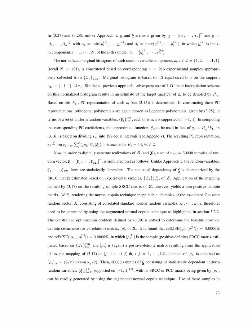
In (3.27) and (3.28), unlike Approach 1, a and b are now given by a = [α1, · · · , αN ]T and b =

[β1, · · · , βN ]T with αi = min(y(1)i , · · · , y(n)

i ) and βi = max(y(1)i , · · · , y(n)

i ), in which y(k)i is the i-

th component, i = 1, · · · , N , of the k-th sample, Yk = [y(k)1 , · · · , y(k)

N ].

The normalized marginal histogram of each random variable component, zi, i ∈ I = {1, 2, · · · , 121}

(recall N = 121), is constructed based on corresponding n = 216 experimental samples appropri-

ately collected from {Zk}nk=1. Marginal histogram is based on 12 equal-sized bins on the support,

szi ≡ [−1, 1], of zi. Similar to previous approach, subsequent use of 1-D linear interpolation scheme

on this normalized histogram results in an estimate of the target marPDF of zi to be denoted by Pzi .

Based on this Pzi , PC representation of each zi (see (3.15)) is determined. In constructing these PC

representations, orthogonal polynomials are again chosen as Legendre polynomials, given by (3.25), in

terms of a set of uniform random variables, {ξi}121i=1, each of which is supported on [−1, 1]. In computing

the corresponding PC coefficients, the approximate function, qi, to be used in lieu of qi ≡ P−1ziPξi

in

(3.16) is based on dividing szi into 199 equal intervals (see Appendix). The resulting PC representation,

zid= limKi→∞

∑Ki

j=0cji Ψj(ξi), is truncated at Ki = 14, ∀i ∈ I.

Now, in order to digitally generate realizations of Z (and Y), a set of nPC = 50000 samples of ran-

dom vector, ξ = [ξ1, · · · , ξ121]T , is simulated first as follows. Unlike Approach 1, the random variables,

ξ1, · · · , ξ121, here are statistically dependent. The statistical dependency of ξ is characterized by the

SRCC matrix estimated based on experimental samples, {Zk}216k=1, of Z. Application of the mapping

defined by (3.17) on the resulting sample SRCC matrix of Z, however, yields a non-positive-definite

matrix, [ρ(1)], rendering the normal copula technique inapplicable. Samples of the associated Gaussian

random vector, X, consisting of correlated standard normal random variables, x1, · · · ,x121, therefore,

need to be generated by using the augmented normal copula technique as highlighted in section 3.2.2.

The constrained optimization problem defined by (3.20) is solved to determine the feasible positive-

definite covariance (or correlation) matrix, [ρ], of X. It is found that relMSE([ρ], [ρ(1)]) = 0.0006%

and relMSE([ρs], [ρ(1)s ]) = 0.0006%, in which [ρ

(1)s ] is the sample (positive-definite) SRCC matrix esti-

mated based on {Zk}216k=1 and [ρs] is (again) a positive-definite matrix resulting from the application

of inverse mapping of (3.17) on [ρ], i.e., (i, j)-th, i, j = 1, · · · , 121, element of [ρs] is obtained as

(ρs)ij = (6/π) arcsin(ρij/2). Then, 50000 samples of ξ consisting of statistically dependent uniform

random variables, {ξi}121i=1, supported on [−1, 1]121, with its SRCC or PCC matrix being given by [ρs],

can be readily generated by using the augmented normal copula technique. Use of these samples in

73

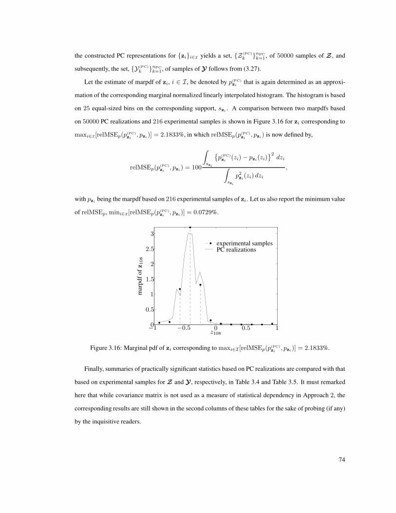
the constructed PC representations for {zi}i∈I yields a set, {Z (PC)

k }nPC

k=1, of 50000 samples of Z , and

subsequently, the set, {Y(PC)

k }nPC

k=1, of samples of Y follows from (3.27).

Let the estimate of marpdf of zi, i ∈ I, be denoted by p(PC)zi

that is again determined as an approxi-

mation of the corresponding marginal normalized linearly interpolated histogram. The histogram is based

on 25 equal-sized bins on the corresponding support, szi . A comparison between two marpdfs based

on 50000 PC realizations and 216 experimental samples is shown in Figure 3.16 for zi corresponding to

maxi∈I[relMSEp(p(PC)zi

, pzi)] = 2.1833%, in which relMSEp(p(PC)zi

, pzi) is now defined by,

relMSEp(p(PC)

zi, pzi) = 100

∫

szi

{p(PC)

zi(zi) − pzi(zi)

}2dzi

∫

szi

p2zi

(zi) dzi

,

with pzi being the marpdf based on 216 experimental samples of zi. Let us also report the minimum value

of relMSEp, mini∈I [relMSEp(p(PC)zi

, pzi)] = 0.0729%.

z108

mar

pd

fo

fz108

experimental samplesPC realizations

−1 −0.500

0.5

0.5

1

1

1.5

2

2.5

3

Figure 3.16: Marginal pdf of zi corresponding to maxi∈I [relMSEp(p(PC)zi

, pzi)] = 2.1833%.

Finally, summaries of practically significant statistics based on PC realizations are compared with that

based on experimental samples for Z and Y , respectively, in Table 3.4 and Table 3.5. It must remarked

here that while covariance matrix is not used as a measure of statistical dependency in Approach 2, the

corresponding results are still shown in the second columns of these tables for the sake of probing (if any)

by the inquisitive readers.

74

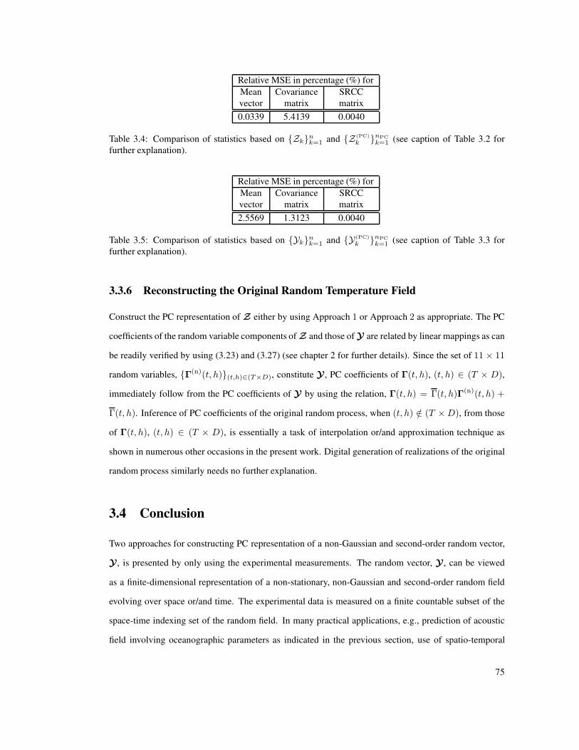
Relative MSE in percentage (%) for

Mean Covariance SRCC

vector matrix matrix

0.0339 5.4139 0.0040

Table 3.4: Comparison of statistics based on {Zk}nk=1 and {Z (PC)

k }nPC

k=1 (see caption of Table 3.2 for

further explanation).

Relative MSE in percentage (%) for

Mean Covariance SRCC

vector matrix matrix

2.5569 1.3123 0.0040

Table 3.5: Comparison of statistics based on {Yk}nk=1 and {Y(PC)

k }nPC

k=1 (see caption of Table 3.3 for

further explanation).

3.3.6 Reconstructing the Original Random Temperature Field

Construct the PC representation of Z either by using Approach 1 or Approach 2 as appropriate. The PC

coefficients of the random variable components of Z and those of Y are related by linear mappings as can

be readily verified by using (3.23) and (3.27) (see chapter 2 for further details). Since the set of 11 × 11

random variables, {Γ(n)(t, h)}(t,h)∈(T×D), constitute Y , PC coefficients of Γ(t, h), (t, h) ∈ (T × D),

immediately follow from the PC coefficients of Y by using the relation, Γ(t, h) = Γ(t, h)Γ(n)(t, h) +

Γ(t, h). Inference of PC coefficients of the original random process, when (t, h) /∈ (T ×D), from those

of Γ(t, h), (t, h) ∈ (T × D), is essentially a task of interpolation or/and approximation technique as

shown in numerous other occasions in the present work. Digital generation of realizations of the original

random process similarly needs no further explanation.

3.4 Conclusion

Two approaches for constructing PC representation of a non-Gaussian and second-order random vector,

Y , is presented by only using the experimental measurements. The random vector, Y , can be viewed

as a finite-dimensional representation of a non-stationary, non-Gaussian and second-order random field

evolving over space or/and time. The experimental data is measured on a finite countable subset of the

space-time indexing set of the random field. In many practical applications, e.g., prediction of acoustic

field involving oceanographic parameters as indicated in the previous section, use of spatio-temporal

75

random field would be a more appropriate model for characterizing the inherent uncertainty in system

parameters of a stochastic system. The PC representation of the random field representing such random

system parameters has been proven to be an efficient tool in systematically propagating the uncertainty to

the model-based predictions of response of the stochastic system.

Approach 1 attempts to capture the complete information of a target mjpdf of Y . This approach

uses the knowledge of a complete set of properly ordered target conditional PDFs estimated from the

experimental measurements and the concept of Rosenblatt transformation. The set of target conditional

PDFs, that uniquely defines the target mjpdf of Y , are approximations, based on linear interpolation, of the

corresponding set of normalized histograms of the appropriate set of experimental samples. Approach 2,

on the other hand, satisfies the target marPDFs and the target SRCC matrix of Y . The set of target

marPDFs and the target SRCC matrix are similarly estimated by using the experimental samples. The

second approach is also founded on the Rosenblatt transformation. In both the approaches, appropriate

functions based on the Rosenblatt transformation are first defined in terms of the selected PC variables,

ξk’s. The defined functions are equal to Y in the sense of distribution. Subsequently, construction of

PC expansion of these functions results in appropriate PC representations that can be readily employed

within the PC framework to propagate the associated uncertainty. It should, however, be realized that the

existences and (if they exist) the true forms of these functions are never known in reality. Nevertheless,

the proposed approaches guarantee [HLD04, Theorem 2.1] that such functions can always be constructed.

For efficient and fast computation of the PC coefficients, the Rosenblatt transformation based functions

are further substituted by the appropriate interpolated functions.

One important distinction between two proposed approaches is that while PC random variables, ξk’s,

are statistically independent in Approach 1, the corresponding set of PC random variables are statistically

dependent in Approach 2. Approach 1 is computationally expensive relative to Approach 2. Additional

model reduction technique, e.g., use of KL decomposition as discussed in the context of numerical illus-

tration in section 3.3.4, is recommended to reduce the computational cost. Further probabilistic assump-

tions as made in section 3.3.4, while modeling the spatio-temporal random temperature field, would also

alleviate the computational burden at the expense of accuracy. But it is certainly recommended if the

achieved accuracy is practically acceptable. Accuracy level of Approach 2 is expected to be higher than

the accuracy level of Approach 1 if additional probabilistic assumptions and model reduction scheme,

as just indicated, are incorporated into Approach 1. Approach 2 would also be computationally cheaper

76

manyfold for low and moderate dimension of Y (quantification of the qualifiers, ‘low’ and ‘moderate’,

however, directly depends on the available computational resources).

77

Chapter 4

Hybrid Representations of Coupled

Nonparametric and Parametric Models

Parametric modeling of stochastic systems has proven useful for systems with well-defined and well

structured sources of uncertainty. The suitability of such models is usually indicated by small levels of

uncertainty associated with their parameters. The parametric model may not efficiently employed to deal

with problems whose level of uncertainty is high, involving spatially distributed sources of uncertainty.

The class of so-called nonparametric stochastic models has recently been introduced in mechanics to

address this specific issue and found to be useful. This chapter presents a coupling technique, adapted to

the receptance frequency response function (FRF) matrix, for combining these two approaches. This will

be useful for the analysis of complex dynamical systems having spatially non-homogeneous uncertainty

that is otherwise difficult to analyze. The existing nonparametric approach was, till date, applied to

the positive definite/semi-definite system matrices, for example, to the matrices of mass, damping and

stiffness. In the current work, the nonparametric approach is also employed to the complex symmetric

receptance FRF matrix, now acting as the system matrix, by having recourse to the Takagi’s factorization.

4.1 Introduction and Motivation

Two types of uncertainty are of particular interest in connection to the dynamical systems: modeling

uncertainty and data uncertainty. Modeling uncertainty can be further decomposed into mechanical

uncertainty and probabilistic uncertainty. While mechanical uncertainty results from several simplified

assumptions in developing a mechanical/mathematical model, referred further here as predictive model,

of the physical phenomena, the latter one stems from the introduction of probabilistic assumptions asso-

ciated with the statistical/probabilistic characteristics of the random system/model parameters (geometry,

boundary conditions, parameters of the constitutive equation etc.) of the predictive model. Examples

78

in which mechanical uncertainty is present include simplified mechanical models of a complex junc-

tion, one or two dimensional beam and plate models instead of their three-dimensional (3D) elasticity

models. Even the 3D theory of elasticity encompasses many assumptions introduced for mathematical

convenience that might not satisfy the ‘true’ behavior of a complex system. The assumption of statistical

independence between two random system parameters and assigning a particular probability distribution

law to a random system parameter are the instances of injecting probabilistic uncertainty. Data uncer-

tainty, on the other hand, is characterized by the uncertainty associated with the data collected from

experimental measurements for estimation of the statistical/probabilistic features of the model parame-

ters. The data limitation (because of finite sample size) and experimental uncertainty (caused due to, for

example, imperfect set-up and condition of the experiment, human error and environmental condition)

introduce data uncertainty.

In addition, the models of certain parts of a complex system are more accurate than those in the other

parts; for instance, the mechanical model of a part constituted of a slender beam structure is generally

better than a simplified mechanical model of a complex joint. This indicates that the uncertainties resulting

from the mechanical model are not homogeneous throughout the system. Uncertainties resulting from the

probabilistic uncertainty are also not spatially homogeneous because, e.g., some of the parameters of a

certain part of the complex system might be truly statistically independent whereas the assumption of

statistical independence for other parameters may be a mere mathematical convenience. Uncertainties

resulting from the data uncertainty are again not spatially homogeneous because the data may not be

uniformly available throughout the complex system. Clearly, in general, uncertainties in a complex system

are expected to be spatially non-homogeneous.

The analysis of a complex dynamical system with such non-homogeneous uncertainties is typically

quite involved both to set-up as well as to numerically resolve. It may not even be possible to analyze

the built-up structure because of the presence of the spatially non-homogeneous uncertainties. In order

to model all the uncertainties in such a complex dynamical systems and to solve the global stochastic

equations, it might be useful and convenient to decompose the system into several smaller subsystems

such that uncertainty in each subsystem is spatially homogeneous. Each of these subsystems can be

analyzed separately using the method most suitable for it, and finally can be assembled to obtain the

response of the built-up system. A subsystem having a lower level of modeling and data uncertainty

79

or/and having a relatively fewer number of random system parameters can be analyzed by using the para-

metric approach requiring knowledge of the local system parameters (for example, Young’s modulus,

shear modulus, bulk modulus, Poisson’s ratio etc.). On the other hand, a subsystem having a higher level

of uncertainties due to modeling uncertainty and data uncertainty or/and having a large number of ran-

dom system parameters can be analyzed by using the recently proposed approach, called nonparametric

approach [Soi00, Soi01a, Soi05a, Soi05b, CLPP+07], that does not require the knowledge of the local

system parameters.

The objective of the work presented in this chapter is to propose a hybrid approach that permits the

coupling between subsystems having been analyzed by using these two different approaches, in order

to determine quantities of interest of the built-up structure. The approach is based on the point-wise

enforcement of dynamic equilibrium condition for each realization of the stochastic system.

4.2 Nonparametric Model

In this section, an overview of Soize’s pioneering work [Soi00, Soi01a], that proposed the nonparametric

approach to model uncertainties in dynamical systems in the low-frequency regime, is provided. This

model differs from the parametric modeling of uncertainties in that it does not require information of the

local parameters of the system being analyzed. The nonparametric framework allows one to construct a

probability density function (pdf) of the random system matrices directly based on partial knowledge of

the systems. It is directed towards constructing the probability models of the random system matrices

without consideration of the parametrization of the dynamical model of the system. The work considers

the problem of constructing the associated probability space, namely,(MS

n(R),F , PA

)in which MS

n(R)

is the set of all real n × n symmetric matrices, F is the σ-algebra of subsets of MSn(R) and PA is

the probability measure on F such that the support of the random system matrix variate is the set of

symmetric positive definite real matrices denoted by M+n (R) ⊂ MS

n(R). It implies that supp(A) =

{A : pA(A) > 0} = M+n (R), where A is the random matrix variate, pA is its pdf, pA : MS

n(R) 7−→

R+ = [0,∞), which can be related to the probability measure, PA, as follows,

dPA(A) = pA(A) dA.

80

Here dA can be interpreted as a volume element in MSn(R) and is defined to be the wedge product or the

exterior product [Fla89] of the independent elements of the differential form of the matrix dA and the

(i, j)th element of dA is simply defined [For08] as dAij in which Aij is the (i, j)th element of A. There

are n(n + 1)/2 such independent elements. In the context of random matrix theory [Meh04, For08],

for symmetric matrix, dA is then given by∧

1≤i≤j≤ndAij , where∧

indicates the wedge product. In

the present context, the wedge product reverts to be the natural volume element,∏

1≤i≤j≤n dAij , in

the Euclidean space Rn(n+1)/2 that is topologically equivalent to MSn(R). Soize, however, considers an

Euclidean structure on MSn(R) to define the following volume element,

dA = 2n(n−1)/4∏

1≤i≤j≤n

dAij ,

that differs by a multiplication factor, 2n(n−1)/4, from the natural volume element. It should be noted that

it is, however, feasible to reformulate the theory behind the nonparametric approach by using the natural

volume element,∏

1≤i≤j≤n dAij , with minor changes (please see section 5.3 for further details).

In constructing the probability measure, the principle of maximum entropy [KK92], as initially intro-

duced by Jaynes [Jay57a, Jay57b] for discrete random variables, has been used [Soi00]. The MaxEnt

principle yields a constrained optimization problem with the objective being to maximize Shannon’s

measure of entropy [Sha48] constrained by the given statistics (mean, variance etc.) of the random variate

representing the available information. In the present case, entropy can be interpreted as a measure of rel-

ative uncertainty [KK92] associated with the probability distribution of the random matrix variate. This

uncertainty is not about which realization of the random matrix variate will be observed but it represents

the uncertainty of the probability distribution of the random matrix variate. The basic idea of the MaxEnt

principle is to choose the probability distribution with maximum uncertainty out of all the probability

distributions that are consistent with the given set of constraints. Any other probability distribution would

be associated with unwarranted assumptions about the systems which are not available [Jay57a, Jay57b].

It should be noted that the uniform distribution is often considered to represent a state of maxi-

mum uncertainty. Interestingly, the probability distribution resulting from the application of Jaynes’s

maximum-entropy (MaxEnt) principle on the continuous pdf [KK92, Section 2.5.2] is the same as the

probability distribution resulting from the use of Kullback-Leibler’s [KL51, Kul59] principle of mini-

mum directed divergence (minimum cross-entropy) provided the prior probability distribution is uniform

81

[SJ80, SJ83, Jay68]. Out of all the probability distributions satisfying the given constraints, the principle

of minimum directed divergence chooses the one that is closest to the uniform distribution. Geometrically,

it corresponds to the probability distribution, in a space consisting of probability distributions (a point in

this space represents a probability distribution), that has minimum directed distance, computed by using

the Kullback-Leibler’s measure [KL51, Kul59], with respect to the point in this space representing the

uniform distribution.

Let us denote the mass matrix of the mean dynamical system by M ∈ M+n (R) and its Cholesky

decomposition [Har97, Theorem 14.5.11] by,

M = LTMLM , (4.1)

in which LM is an upper triangular matrix in the set, Mn(R), of all real matrices of size n× n, where n

is the total degree of freedoms (dof) of the mean finite element model (FEM). The mean stiffness matrix

K is positive definite for a fixed structure and positive semi-definite for free structure and consequently

has the following Cholesky decomposition [Har97, Theorem 14.5.16],

K = STKSK ,

in which SK is an upper triangular matrix in Mn(R) with a fixed structure and is an almost upper trian-

gular matrix in Mm,n(R) for free structure with (n −m) ≤ 6 being the number of rigid body modes of

the system; where Mm,n(R) is the set of all real matrices of size m×n. The random system mass matrix

M and random system stiffness matrix K are then written as [Soi99],

M = LTMGMLM , and K = ST

KGKSK ,

in which GM and GK are second order (see below (4.4)) random matrix variate, respectively, in M+n (R)

and M+m(R) with E {GM} = In and E {GK} = Im, where E is the mathematical expectation operator

and Ip is an identity matrix of size p × p, p = n,m. A similar decomposition exists for random system

damping matrix.

Next step is to generate the ensembles of the random matrices GM and GK in order to simulate the

realizations of M and K. Let us denote the random matrix to be generated (GM , GK or the corresponding

82

matrix for damping) by A ∈ M+n (R) generically. The pdf, pA, is then determined by using the principle

of maximum entropy. The nonparametric approach as proposed by Soize only assumes the information of

the ensemble means of the system matrices (mass, stiffness and damping matrices) to be known a priori.

These ensemble means can be taken as the system matrices obtained by discretizing a nominal continuous

system in view of analyzing it using the finite element method (FEM). Subsequent uses of

1. (normalization constraint) the axioms of probability, specifically that the total probability must

be unity,

2. (ensemble mean constraint) the given ensemble mean matrix, A, that is given by the matrix cor-

responding to the mean system, and

3. (existence of moments of response) the existence of the moments of the response random vari-

ables, that is expressed in terms of the existence of the moments of the random system matrices,

as constraints in the MaxEnt principle yields the pdf, pA. Here, the last constraint also implies that

[Soi01a, p. 1985],

E{‖A−1‖γ

F

}<∞, for mass, damping and stiffness matrices,

where γ ≥ 1 is a positive integer and ‖ · ‖F is the Frobenius norm defined by ‖A‖F = 〈A,AT 〉1/2 ≡{tr(AAT

)}1/2=(∑

ij |aij |2)1/2

, in which aij is the (i, j)-th element of A. The existence of these

moments is required in order to guarantee the existence of moments of the response that is obtained by

solving a dynamical system, for example, AX = F ⇒ X = A−1F, in which X and F, respectively,

represent the response of and the external disturbance on the stochastic system represented by the random

matrix operator A. Subsequently, the pdf, pA, can be determined [Soi00, Soi01a] by maximizing the

entropy of pA subject to the above constraints.

The pdf, pA, thus obtained is found to be characterized by three parameters,A, λ and n. Here, (1−λ)

is one of the Lagrange multipliers, with λ > 0, associated with the last constraint. When A is identity

matrix (as is the case for GM and GK), λ is given by [Soi01a],

λ =(1 − δ2A)

2δ2An+

1 + δ2A2δ2A

, (4.2)

83

where δA > 0 is the dispersion parameter defined by,

δA =

{E{‖A−A‖2

F

}

‖A‖2F

}1/2

. (4.3)

From the convergence study and existence of the second order moment of the inverse random matrix

(guaranteing the existence of moments of the response random variables), δA must satisfy the following

relation [Soi01a],

0 < δA <

√n0 + 1

n0 + 5, ∀n ≥ n0, (4.4)

in which n0 is an integer. This condition then guarantees the existence of the mean and the second order

moment of A−1 (as required for the random matrices associated with mass, damping and stiffness). The

upper bound of δA in (4.4) is a monotonically and strictly increasing function of n0 with min√

n0+1n0+5 =

0.5774 for n0 = 1 and sup√

n0+1n0+5 = 1. In the context of practical problems, n ≥ 1, and δA typically

satisfies the relation expressed by (4.4) implying λ≫ 1 by (4.2).

The PDF associated with MaxEnt pdf is the Wishart distribution or matrix-variate gamma distribu-

tion, W(

1n−1+2λA, (n− 1 + 2λ)

)(see, e.g., [Mur82, Section 3.2], [GN00, Chapter 3] [And03, Sec-

tion 7.2]). Procedures for generations of realizations of random matrix A are well documented in the

literature [Mur82, Theorem 3.2.5], [GN00, Theorem 3.3.1 or Theorem 3.3.11] and used extensively by

Soize [Soi00, Soi01a] to describe the simulation technique for sampling from the Wishart distribution. A

quick summary, as to how Monte Carlo simulation (MCS) technique is employed to generate the realiza-

tions of A, is provided below. (See pp. 116–117 for further theoretical and algorithmic details).

4.2.1 Monte Carlo Simulation of A

For many applications, n is sufficiently large and in such cases, there exists a simple form of the random

matrix, A, given by,

A =1

mA

mA∑

j=1

(LT

AUj

) (LT

AUj

)T, (4.5)

Here, LA is defined by the Cholesky decomposition of A, i.e., A = LTALA, Uj ’s are independent and

identically distributed (i.i.d) Rn-valued normal random vector, i.e., N (0, In), and finally, mA = (n +

1)/δ2A. This form is more amenable to the practical calculation for the purpose of MCS of the random

matrix, A.

84

The form defined by (4.5) is useful when λ is an integer implying that mA is also an integer. For

high n, mA can be rounded off to the nearest integer without causing significant limitation in the non-

parametric model. However, this introduces probabilistic uncertainty in the model. To avoid introducing

this probabilistic uncertainty (though very small), the exact simulation technique can be used ifmA is not

integer. WhenmA is not an integer, simulation of A involves simulation of Gamma random variables and

Gaussian random variables (see Algorithm 5.3.3 in pp. 116).

It should be noted here that the above nonparametric formulation is developed by following a sim-

ilar procedure for constructing a probability space for Gaussian orthogonal ensemble (GOE) [Meh04].

However, unlike the statistically independent elements of matrix belonging to GOE, the elements Aij

of the random matrix A ∈ M+n (R) are not statistically independent. A comparative study by using the

ensemble of the matrix computed in the framework of the nonparametric approach and the matrix of GOE

has been conducted to show the superiority of the nonparametric approach over the GOE approach in the

context of structural dynamics problems [Soi03]. This work also compares the nonparametric approach

and the parametric approach to validate the nonparametric technique in the low-frequency range. The

nonparametric approach has been applied both to problems of frequency domain [Soi00, Soi03] and time

domain [Soi01a, Soi01b].

This section is concluded by noting that given the partial information separately for each of the sys-

tem matrices with no information of the statistical dependency among these system matrices, the Max-

Ent principle also implies that these system matrices are statistically independent of each other, i.e.,

pM,C,D,K(M,C,D, K) = pM(M) pC(C) pD(D) pK(K) [Soi00]. Here C and D, respectively, rep-

resent the matrix of viscous damping and structural damping and C and D are their realizations. The

resulting fact of this independence is discernible because no knowledge of the statistical dependency of

the random system matrix variate, M,C,D,K, has been used in the development. Only knowledge of the

ensemble means of these matrices are separately incorporated in the formulation while solving a dynam-

ical system. In section 4.3, this implied condition of statistical independency on the system matrices is

removed by considering the complex FRF matrix of the system at the expense of additional computational

burden. Use of FRF matrix, instead of mass, stiffness and damping matrices, automatically takes care of

the issue of statistical dependency among the mass, stiffness and damping matrices of the system.

85

4.3 Nonparametric Model for Complex FRF Matrix

The receptance FRF matrix, H(ω), is expressed by,

H(ω) =(K − ω2M + ι(ωC +D)

)−1,

where K , M , C and D are, respectively, the system matrices of stiffness, mass, viscous damping and

structural damping, ω is the forcing frequency and ι =√−1. Here,H(ω) is a complex symmetric matrix

and consequently, has the following Takagi’s factorization [HJ85, Corollary. 4.4.4],

H(ω) = UΣUT , (4.6)

where U ∈ U(n) is a unitary matrix with U(n) being the unitary group of unitary matrices of size n× n.

The set of orthonormal eigenvectors of H(ω)H(ω)∗ constitutes the columns of U and the positive square

roots of the corresponding eigenvalues of H(ω)H(ω)∗ are the corresponding diagonal entries of Σ. Here

∗ represents the element-wise conjugate operator. The Takagi’s factorization for a complex symmetric

matrix is a special case of singular value decomposition (SVD) for symmetric matrix. The SVD exists

for any matrix A ∈ Mm,n(C) (where Mm,n(C) is the set of all complex matrices of size m × n) such

that A = UΣW † with U ∈ U(m) and W ∈ U(n) being unitary matrices and the diagonal entries of the

diagonal matrix, Σ, being the non-negative square roots of the eigenvalues of AA† (where † represents

the conjugate-transpose operator). In Takagi’s factorization for complex symmetric matrix, it turns out

that U = W ∗. Now, at any fixed ω, define A = H(ω)H(ω)∗. As H(ω) is symmetric, H(ω)∗ = H(ω)†.

Consequently, A = A† is Hermitian and also positive definite because x†Ax = x†H(ω)H(ω)∗ x =(H(ω)†x

)† (H(ω)†x

)= ‖H(ω)†x‖2

2 > 0 ∀ non-zero x ∈ Cn. Here ‖ · ‖2 is Euclidean norm on Cn.

Therefore, all the eigenvalues of H(ω)H(ω)∗ are positive. If we denote the group of all the diagonal

matrices of size n× n with positive diagonal entries by D+n , then Σ ∈ D+

n ⊂ M+n (R). Note that (4.6) can

also be written as H(ω) = V TV where V = (UΣ1/2)T with Σ1/2 = diag(+√σ1, · · · ,+

√σn) in which

σj is the j-th diagonal element of Σ. Hence, the receptance FRF matrix of the mean dynamical system

H(ω) has the following decomposition,

H(ω) = V TH(ω)VH(ω)

86

which can be compared to (4.1). Now, the random receptance FRF matrix, H(ω), can be written as,

H(ω) = V TH(ω)GH(ω)VH(ω) (4.7)

in which GH(ω) is the random matrix variate (with all of its moments being finite) in M+n (R) and

E{GH(ω)

}= In. The last constraint condition on “existence of moments of response” as mentioned

earlier also guarantees the existence of the moments of A implying [Soi01a, p. 1985],

E {‖A‖γF} <∞, for receptance FRF matrix,

as required for the random matrix associated with the receptance FRF matrix in order to enforce the

condition for the existence of random response quantity.

Then, a probability model for GH(ω) can be developed in exactly the same way as described earlier for

GM and GK in section 4.2. Simulation of GH(ω), and therefore, of H(ω), follows from the constructed

probability model of GH(ω) by virtue of (4.7).

The additional computation burden of this FRF-based nonparametric formulation due to different

probability model of H(ω) at different values of ω in the frequency band of interest must be noted as

a computational drawback. However, the question of statistical independent mass, damping and stiff-

ness matrices does not arise in this case since the FRF matrix, that depends on these mass, damping and

stiffness matrices, is alternately being characterized. This FRF-based nonparametric formulation is also

more suitable from practical consideration because experimental measurement is directly available on

the FRF matrix not on the mass, damping or stiffness matrices. In this case, there exists no modeling

uncertainty since the ‘true’ physical process is directly measured. However, there do exists experimen-

tal/measurement uncertainty that is now characterized within the nonparametric formalism along with the

inherent or irreducible uncertainty in the ‘true’ process.

87

4.4 Coupling Nonparametric Model and Parametric Model

The coupling technique used in the current work to combine the nonparametric model and the parametric

model is based on the receptance FRF matrices of the uncoupled subsystems. The standard FRF coupling

technique for two subsystems (say, denoted by a and b) is expressed by [JBF88],

aaH acH abH

caH ccH cbH

baH bcH bbH

=

H(a)rr H

(a)rc 0

H(a)cr H

(a)cc 0

0 0 H(b)rr

−

H(a)rc

H(a)cc

−H(b)rc

[H

(a)cc + H

(b)cc

]−1

H(a)rc

H(a)cc

−H(b)rc

T

. (4.8)

The left-hand-side represents the whole FRF matrix of the built-up system which consists of the two

subsystems, a and b. This FRF matrix is partitioned such that each partition can be expressed by the FRF

matrices of the uncoupled subsystems a and b as shown in the right-hand-side (rhs). The FRF matrices

of the uncoupled subsystems are denoted by H(j)·· , j = a, b. The subscript, c, of these FRF matrices

denotes the coupling dof involved in the common physical connection of the subsystems, a and b, and

the subscript, r, represents the remaining internal dof of the corresponding subsystems, a and b. The

built-up FRF matrix must be symmetric and so, we have the relations, caH = acHT , baH = abH

T and

bcH = cbHT , that can be realized upon expressing each partition of the built-up FRF matrix in terms of

the FRF matrices of the uncoupled subsystems, H(a)·· ’s and H

(b)·· ’s. This basic approach, however, is not

directly adapted to joints with more than two components, and enhancements have been proposed in the

literature [Urg91, RB95, SK97, Liu00, LL04]. One such method has already been used by the author in

the context of a different class of vibration problem [DM03] and would be used in the current work. A

description of this coupling technique follows next.

Consider the mean built-up system consisting of several subsystems. Also consider one constituent

subsystem. Denote this subsystem by j and the complex FRF matrix of the subsystem by H(j)(ω) when

it is isolated from the other adjoining subsystems of the built-up structure. The procedure of construction

of the matrix, H(j)(ω), is not relevant in the coupling technique described here. The receptance FRF

88

matrix can be constructed by using any available technique, for example, modal analysis, direct inversion

of the dynamic stiffness matrix (DSM) of the corresponding uncoupled finite element model, or even

by experimentally identifying this FRF matrix. It should be noted here that the subsystem, j, could be

either classically or non-classically damped and viscously or hysteretically damped. We need to adopt an

appropriate method to analyze the subsystem in order to compute H(j)(ω). Given H(j)(ω), the response

of the subsystem in frequency domain can be obtained from the following equation,

X(j)(ω) = H(j)(ω)F (j)(ω), (4.9)

where X(j)(ω) =[X

(j)1 X

(j)2 · · · X(j)

nj

]T∈ Cnj is the response of subsystem j, where nj is

the total number of dof (displacements or/and rotations) of the subsystem, j. Similarly, F (j)(ω) =[F

(j)1 F

(j)2 · · · F (j)

nj

]T∈ C

nj is the vector of forcing components (including the coupling forces and

the externally applied forces) at the nj dof, when the subsystem, j, is isolated from the other adjoining

subsystems. Then,H(j)(ω) is an nj ×nj complex symmetric matrix. The (s, t)-th element of this matrix,

H(j)s,t (ω), represents the response (displacement/rotation) of the subsystem j at the frequency ω at the s-th

dof due to an unit force (load/moment) acting at t-th dof.

Let all the excitation points on subsystem j be denoted by (I , · · · , Z) and all the coupling points

by (I, · · · , Z). Consider one of these coupling points denoted by k, k ∈ (I, · · · , Z). Also suppose

that there are Nk number of subsystems denoted by (j, l, · · · , s) connected at this coupling point, k.

In addition, consider that at this coupling point, there are total pk number of dof (pk ≤ 6) that must

maintain the continuity of the corresponding responses among the subsystems, (j, l, · · · , s), meeting at

the coupling point. For subsystem j, let us denote these dof that would generate either a coupling force

or a coupling moment at the coupling point, k, when the subsystem j would be isolated from the other

adjoining subsystems, bymj(ok), ok = 1, 2, · · · , pk. The response at the dof,mj(ok), ok = 1, 2, · · · , pk,

then can be expressed by,

X(j)mj(ok)(ω) =

nj∑

r=1

H(j)mj(ok),r(ω)F (j)

r (ω) (4.10)

It should be noted here that the force components, F (j)r (ω) contain both the known externally applied

forces and the unknown coupling forces resulting from the isolation of the subsystem j from the other

adjoining subsystems, (l, · · · , s). Hence it is useful to decompose the right hand side of (4.10) into two

89

parts — one containing the contributions from the known components of the externally applied forces and

the other containing the contributions from the unknown coupling forces. This is done next.

Let Sj be the set containing the dof associated with the unknown coupling force components for sub-

system j, Sj = {mj(ok), ok = 1, 2, · · · , pk, k ∈ (I, · · · , Z)}. If we denote the total number of dof

(at an excitation point, q, q ∈ (I , · · · , Z)), that are associated with the non-zero externally applied

known force components, by pq (pq ≤ 6) and the corresponding dof by mj(oq), oq = 1, 2, · · · , pq,

we have Sj ={mj(oq), oq = 1, 2, · · · , pq, q ∈ (I , · · · , Z)

}. As there are a total Nk number of sub-

systems, (j, l, · · · , s), connected at the coupling point k, one can write a total Nk number of expres-

sions of response for each dof at this point. Now during the process of assembling the subsys-

tems, we need to merge the appropriate dof of their coupling points. For convenience, we sort the

elements of the sets of the dof of the subsystems, (j, l, · · · , s), connected at the coupling point k,

{mj(ok), ok = 1, 2, · · · , pk} , {ml(ok), ok = 1, 2, · · · , pk} , · · · , {ms(ok), ok = 1, 2, · · · , pk}, such

that the ok-th element of each of the sets, mi(ok), i = j, l, · · · , s, ∀ ok = 1, 2, · · · , pk, refers to the same

dof of the assembled structure. Hence, from the condition of compatibility of the response at the merged

dof of the assembled system, following (Nk − 1) number of equations can be formed (after performing

some rearrangement-type operations) for each ok, ok = 1, 2, · · · , pk,

∑

r∈Sj

H(j)mj(ok),r(ω)F (j)

r (ω) −∑

r∈Sl

H(l)ml(ok),r(ω)F (l)

r (ω)

= −∑

r∈Sj

H(j)mj(ok),r(ω)F

(j)r (ω) +

∑

r∈Sl

H(l)ml(ok),r(ω)F

(l)r (ω)

· · · · · · 1-st equation

...

∑

r∈Sj

H(j)mj(ok),r(ω)F (j)

r (ω) −∑

r∈Ss

H(s)ms(ok),r(ω)F (s)

r (ω)

= −∑

r∈Sj

H(j)mj(ok),r(ω)F

(j)r (ω) +

∑

r∈Ss

H(s)ms(ok),r(ω)F

(s)r (ω)

· · · · · · (Nk − 1)-th equation. (4.11)

Here, subsystem, l, contains (P, · · · , T ) coupling points (with k ∈ (P, · · · , T )) and (P , · · · , T )

exciting points, and subsystem, s, contains (S, · · · , U) coupling points (with k ∈ (S, · · · , U))

and (S, · · · , U) exciting points so that Sl = {ml(ok), ok = 1, 2, · · · , pk, k ∈ (P, · · · , T )}, Sl =

90

{ml(oq), oq = 1, 2, · · · , pq, q ∈ (P , · · · , T )}

, Ss = {ms(ok), ok = 1, 2, · · · , pk, k ∈ (S, · · · , U)} and

Ss = {ms(oq), oq = 1, 2, · · · , pq, q ∈ (S, · · · , U)}

.

It should be noted that rhs of this set of equations are completely known since it contains the known

external loads acting on the subsystems. The unknown is the coupling force vector denoted by the con-

catenated column vector,[F

(j)Sj

F(l)Sl

· · · F(s)Ss

]T, of the column vectors, (F

(t)St

)T , t ∈ (j, l, · · · , s), that

consist of the force components F (t)r , r ∈ St, t ∈ (j, l, · · · , s). Set of equations, similar to (4.11), are

further developed, in a similar manner, for all the coupling points of the built-up structure.

The next step is to consider the force equilibrium conditions of coupling forces (loads and moments)

of different subsystems at a common dof. For coupling point, k, as the dof, mj(ok), ml(ok),· · · and

ms(ok), ∀ ok = 1, 2, · · · , pk, refer to the same dof of the assembled structure (because we choose to

sorted them in this fashion), we have the following force equilibrium condition at the coupling point k,

F(j)mj(ok)(ω) + F

(l)ml(ok)(ω) + · · · + F

(s)ms(ok)(ω) = 0, ok = 1, 2, · · · , pk. (4.12)

In this manner, it is possible to form the force equilibrium conditions of the coupling forces at all the

coupling points of the assembled structure.

The sets of equations representing the deflection compatibility conditions (see (4.11)) at all the cou-

pling points lead to a total of∑Nc

k=1[Nk − 1]Dk equations. Here, Nc is the total number of coupling

points in the assembled system, Nk, Nk ≥ 2, is the number of subsystems coupled at the coupling point

k, k = 1, 2, · · · , Nc and Dk, Dk ≤ 6, is the total number of dof that would generate either a coupling

load or a coupling moment at the coupling point, k, when one of the subsystems connected at the cou-

pling point would be isolated from the other adjoining subsystems. The sets of equations representing

the force equilibrium conditions (see (4.12)) at all the coupling points of the assembled system result

in a total of∑Nc

k=1Dk equations. Consequently, there is a total of∑Nc

k=1NkDk equations representing

the deflection compatibility and the force equilibrium conditions. On the other hand, there is a total of

∑Nc

k=1NkDk unknown coupling force components denoted by the unknown concatenated coupling force

vector[F

(1)S1

F(2)S2

· · · F (j)Sj

F(l)Sl

· · · F(s)Ss

· · · F (Ns)SNs

]Twith Ns being the total number of subsystems

into which the built-up structure is decomposed. This unknown coupling force vector can be readily

obtained by solving the above equations representing the deflection compatibility and the force equilib-

rium conditions. Having calculated all the coupling forces at all the coupling points, the response of

91

any subsystem, j, can be readily computed by using (4.9), X(j)(ω) = H(j)(ω)F (j)(ω). Though the

procedure is described for mean built-up system, it remains precisely the same if applied to any other

realization of the ensemble of the built-up systems. Therefore, the formulation can be applied to each

realization of the ensemble of the systems to compute the ensemble of the responses which can be fur-

ther processed to evaluate the statistics of the response quantities of interests. This procedure results in

dynamic equilibrium of the stochastic system being satisfied sample-wise.

This coupling technique allows one to treat a complex dynamical structure as being formed of several

simple subsystems, each of which could be analyzed individually and independently of others without

having recourse to the global mode shapes of the built-up structure. Analysis of each constituent sub-

system is performed by using a method that is most adapted to it. Assemblage of all such analyses at

subsystem level results in equations for the built-up structure. This coupling technique requires, as inputs,

the subsystems’ FRFs over a given frequency range and produces the output of the built-up system. Basic

output of this technique is the displacement field from which other response quantities, i.e., velocity,

acceleration, stress and strain fields could be readily obtained.

The formulation is exemplified by considering a structure that consists of a set of three free-free Euler-

Bernoulli beam (parametric) subsystems that are discretely coupled by a set of six axially vibrating rod

(nonparametric) subsystems.

4.5 Illustration and Discussion on Results

Consider the built-up structure shown in Figure 4.1. Subsystems 2, 3, 4, 6, 7 and 8 are analyzed by using

nonparametric approach and subsystems 1, 5 and 9 are analyzed by using parametric approach to com-

pute the respective realizations of FRFs of the uncoupled subsystems. These computed FRFs are used to

determine the realizations of the response of the built-up structure. The parametric subsystems are mod-

eled as Euler-Bernoulli beams and the mean subsystems of all the connecting nonparametric subsystems

are modeled as axially vibrating rods. The parametric subsystems are analyzed by using the classical

dynamic analysis for continuous systems and subsequently, lowest 10 modes (including the 2 rigid-body

modes) of each subsystem have been retained to compute the realizations of the FRFs by using the modal

superposition method. On the other hand, the mass and stiffness matrices of the mean nonparamet-

ric subsystems are computed by using commercially available finite element analysis (FEA) software,

92

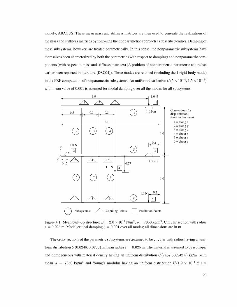
namely, ABAQUS. These mean mass and stiffness matrices are then used to generate the realizations of

the mass and stiffness matrices by following the nonparametric approach as described earlier. Damping of

these subsystems, however, are treated parametrically. In this sense, the nonparametric subsystems have

themselves been characterized by both the parametric (with respect to damping) and nonparametric com-

ponents (with respect to mass and stiffness matrices) (A problem of nonparametric-parametric nature has

earlier been reported in literature [DSC04]). Three modes are retained (including the 1 rigid-body mode)

in the FRF computation of nonparametric subsystems. An uniform distribution U(5× 10−4, 1.5× 10−3)

with mean value of 0.001 is assumed for modal damping over all the modes for all subsystems.

1.9

0.5

1.0 N

1.0 Nm

1.0 Nm

1.0 N

2.1

0.3 0.3 1

3 4

6

2

5

7 8

1.0 N0.2

0.2

1

2 3

5

1 3 5

2 4

Copuling Points;Subsystems; Excitation Points

4

0.27 6

1.1 N

7 8 9 9

1 = along x

2 = along y

3 = along z

4 = about x

5 = about y

6 = about z

1.0

1.0

force and momentdisp, rotation,Conventions for

0.17

y

z

x

Figure 4.1: Mean built-up structure;E = 2.0×1011 N/m2, ρ = 7850 kg/m3, Circular section with radius

r = 0.025 m, Modal critical damping ξ = 0.001 over all modes; all dimensions are in m.

The cross-sections of the parametric subsystems are assumed to be circular with radius having an uni-

form distributionU(0.0248, 0.0253) m mean radius r = 0.025 m. The material is assumed to be isotropic

and homogeneous with material density having an uniform distribution U(7457.5, 8242.5) kg/m3 with

mean ρ = 7850 kg/m3 and Young’s modulus having an uniform distribution U(1.9 × 1011, 2.1 ×

93

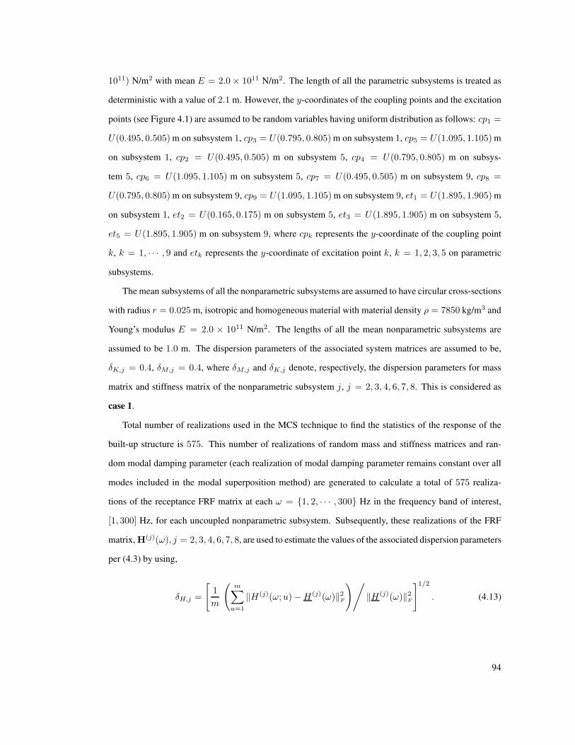
1011) N/m2 with mean E = 2.0 × 1011 N/m2. The length of all the parametric subsystems is treated as

deterministic with a value of 2.1 m. However, the y-coordinates of the coupling points and the excitation

points (see Figure 4.1) are assumed to be random variables having uniform distribution as follows: cp1 =

U(0.495, 0.505) m on subsystem 1, cp3 = U(0.795, 0.805) m on subsystem 1, cp5 = U(1.095, 1.105) m

on subsystem 1, cp2 = U(0.495, 0.505) m on subsystem 5, cp4 = U(0.795, 0.805) m on subsys-

tem 5, cp6 = U(1.095, 1.105) m on subsystem 5, cp7 = U(0.495, 0.505) m on subsystem 9, cp8 =

U(0.795, 0.805) m on subsystem 9, cp9 = U(1.095, 1.105) m on subsystem 9, et1 = U(1.895, 1.905) m

on subsystem 1, et2 = U(0.165, 0.175) m on subsystem 5, et3 = U(1.895, 1.905) m on subsystem 5,

et5 = U(1.895, 1.905) m on subsystem 9, where cpk represents the y-coordinate of the coupling point

k, k = 1, · · · , 9 and etk represents the y-coordinate of excitation point k, k = 1, 2, 3, 5 on parametric

subsystems.

The mean subsystems of all the nonparametric subsystems are assumed to have circular cross-sections

with radius r = 0.025 m, isotropic and homogeneous material with material density ρ = 7850 kg/m3 and

Young’s modulus E = 2.0 × 1011 N/m2. The lengths of all the mean nonparametric subsystems are

assumed to be 1.0 m. The dispersion parameters of the associated system matrices are assumed to be,

δK,j = 0.4, δM,j = 0.4, where δM,j and δK,j denote, respectively, the dispersion parameters for mass

matrix and stiffness matrix of the nonparametric subsystem j, j = 2, 3, 4, 6, 7, 8. This is considered as

case 1.

Total number of realizations used in the MCS technique to find the statistics of the response of the

built-up structure is 575. This number of realizations of random mass and stiffness matrices and ran-

dom modal damping parameter (each realization of modal damping parameter remains constant over all

modes included in the modal superposition method) are generated to calculate a total of 575 realiza-

tions of the receptance FRF matrix at each ω = {1, 2, · · · , 300} Hz in the frequency band of interest,

[1, 300] Hz, for each uncoupled nonparametric subsystem. Subsequently, these realizations of the FRF

matrix, H(j)(ω), j = 2, 3, 4, 6, 7, 8, are used to estimate the values of the associated dispersion parameters

per (4.3) by using,

δH,j =

[1

m

(m∑

u=1

‖H(j)(ω;u) −H(j)(ω)‖2F

)/‖H(j)(ω)‖2

F

]1/2

. (4.13)

94

Here, m = 575 and H(j)(ω;u), u = 1, · · · ,m, is the u-th realization of H(j)(ω). The results are plotted

in Figure 4.2. It can be seen that the dispersion parameter of random FRF matrix of each uncoupled

nonparametric subsystem remains almost constant over the frequency range of interest, [1, 300] Hz, and

consequently, δH,2 = 0.2513, δH,3 = 0.2542, δH,4 = 0.2462, δH,6 = 0.2406, δH,7 = 0.2510 and

δH,8 = 0.2799 have been considered in the second phase of analysis (case 2) when realizations of the

random recptance FRF matrices of the nonparametric subsystems are generated instead of generating the

realizations of the random mass and stiffness matrices and random modal damping parameters of the non-

parametric subsystems. In this second case, the subsystems 2, 3, 4, 6, 7 and 8 are precisely characterized

ω (Hz)

δ H,j

j = 2j = 3j = 4j = 6j = 7j = 8

0 50 100 150 200 250 3000.24

0.245

0.25

0.255

0.26

0.265

0.27

0.275

0.28

Figure 4.2: Dispersion parameters of receptance FRF matrices of nonparametric subsystems.

by the nonparametric model unlike the first case. The mean matrices of H(j)(ω), j = 2, 3, 4, 6, 7, 8, in

the second case are considered to be the same as the mean matrices of the FRF matrices (calculated based

on the mean mass and stiffness matrices and mean modal damping parameter considered in case 1) in

the first case. The characteristics of the random parameters of the parametric subsystems in the second

95

case are considered to be the same as the respective characteristics in the first case. Again, a total of 575

realizations of the built-up system are generated to use in the MCS technique in the second case.

Based on 575 realizations of the receptance FRF matrices of each uncoupled subsystems in the fre-

quency band [1, 300] Hz for each case, a total of 575 realizations of the responses of the built-up structure

for each case is computed by using the coupling technique as described earlier.

ω (Hz)

Sta

tist

ics

of

resp

on

se

| Sample mean of W3,1 || W3,1 of mean system|max(| W3,1 |)min(| W3,1 |)σW3,1

0 50 100 150 200 250 300

10

10

10

10

10

10

10

10

10

−2

−3

−4

−5

−6

−7

−8

−9

−10

Figure 4.3: Statistical details of the deflection, W3,1, of the built-up structure (case 1).

Use of these 575 realizations of the response of the built-system yields Figure 4.3 and Figure 4.4

showing the statistics of the response |W3,1| of the built-up system, respectively, for case 1 and case 2. In

this figures, |·| represents the magnitude of the response andWm,k represents the displacement or rotation

denoted by m,m = 1 · · · , 6, (according to the convention described in Figure 4.1) at the coupling point

k, k = 1, · · · , 9. It can be seen that all the statistics (sample mean, sample standard deviation, sample

maximum and sample minimum) of the displacement along z direction at coupling point 1 computed

in both the cases match very closely. In this figures, the response of the mean built-up system is also

superimposed. It is noted that the response (same for both the cases) of the mean system usually lies in

the interval bounded by the sample maximum and sample minimum except in the frequency range 50 −

75 Hz near anti-resonance for both the cases. The responses of the built-up system near a few resonance

96

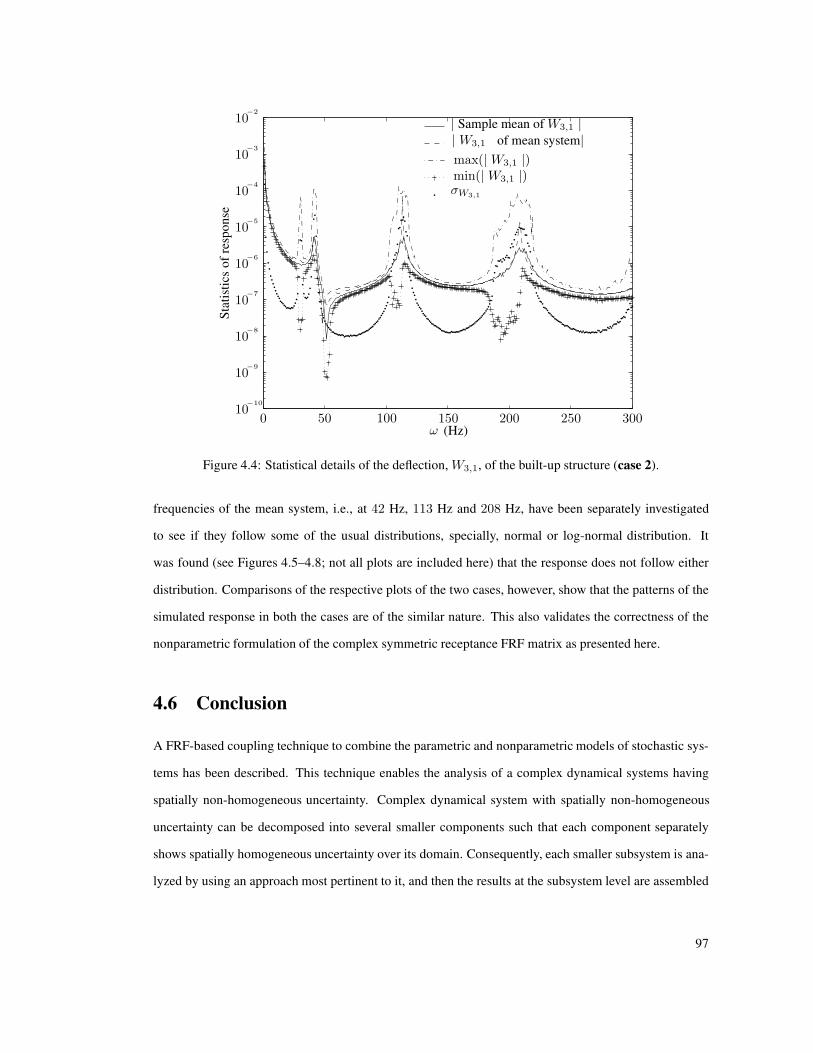
ω (Hz)

Sta

tist

ics

of

resp

on

se

| Sample mean of W3,1 || W3,1 of mean system|max(| W3,1 |)min(| W3,1 |)σW3,1

0 50 100 150 200 250 300

10

10

10

10

10

10

10

10

10

−2

−3

−4

−5

−6

−7

−8

−9

−10

Figure 4.4: Statistical details of the deflection, W3,1, of the built-up structure (case 2).

frequencies of the mean system, i.e., at 42 Hz, 113 Hz and 208 Hz, have been separately investigated

to see if they follow some of the usual distributions, specially, normal or log-normal distribution. It

was found (see Figures 4.5–4.8; not all plots are included here) that the response does not follow either

distribution. Comparisons of the respective plots of the two cases, however, show that the patterns of the

simulated response in both the cases are of the similar nature. This also validates the correctness of the

nonparametric formulation of the complex symmetric receptance FRF matrix as presented here.

4.6 Conclusion

A FRF-based coupling technique to combine the parametric and nonparametric models of stochastic sys-

tems has been described. This technique enables the analysis of a complex dynamical systems having

spatially non-homogeneous uncertainty. Complex dynamical system with spatially non-homogeneous

uncertainty can be decomposed into several smaller components such that each component separately

shows spatially homogeneous uncertainty over its domain. Consequently, each smaller subsystem is ana-

lyzed by using an approach most pertinent to it, and then the results at the subsystem level are assembled

97

|W3,1 |

Pro

bab

ilit

y

0 2 4 6 8 10 12

×10−5

0.0010.003

0.010.02

0.050.10

0.25

0.50

0.75

0.900.95

0.980.99

0.9970.999

Figure 4.5: Normal probability plot of |W3,1| at ω = 42 Hz (case 1).

|W3,1 |

Pro

bab

ilit

y

0 2 4 6 8 10 12

×10−5

0.0010.003

0.010.02

0.050.10

0.25

0.50

0.75

0.900.950.980.99

0.9970.999

Figure 4.6: Normal probability plot of |W3,1| at ω = 42 Hz (case 2).

by using the coupling technique described here to obtain the response quantities of interest at the built-up

system level. The FRFs associated with the uncoupled subsystems as required in this coupling technique

98

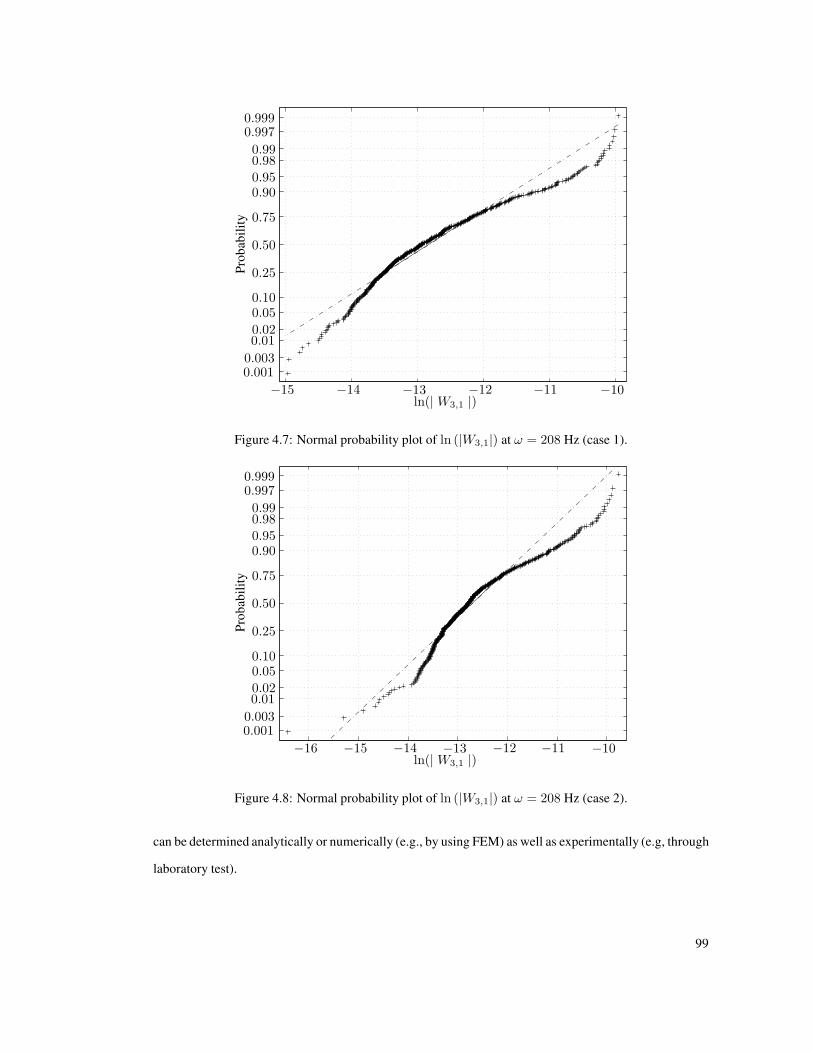
ln(| W3,1 |)

Pro

bab

ilit

y

−15 −14 −13 −12 −11 −10

0.0010.003

0.010.02

0.050.10

0.25

0.50

0.75

0.900.95

0.980.99

0.9970.999

Figure 4.7: Normal probability plot of ln (|W3,1|) at ω = 208 Hz (case 1).

ln(| W3,1 |)

Pro

bab

ilit

y

−16 −15 −14 −13 −12 −11 −10

0.0010.003

0.010.02

0.050.10

0.25

0.50

0.75

0.900.95

0.980.99

0.9970.999

Figure 4.8: Normal probability plot of ln (|W3,1|) at ω = 208 Hz (case 2).

can be determined analytically or numerically (e.g., by using FEM) as well as experimentally (e.g, through

laboratory test).

99

Not only the usual real positive definite/semi-definite mass, stiffness and damping matrices can be

modeled within the framework of the nonparametric approach, it is also shown here that the nonparametric

formulation can also be employed to model the uncertainty in the complex symmetric FRF matrix of the

system. More generally, even if any system matrix does not show any symmetry (e.g., rotating systems

having skew-symmetric damping matrix or/and skew-symmetric stiffness matrix), it can be effectively

dealt with by using the nonparametric approach by having recourse to the SVD that exists for any matrix

A ∈ Mm,n(C).

100

Chapter 5

A Bounded Random Matrix Approach

All fixed set patterns are incapable of adaptability or pliability.

The truth is outside of all fixed patterns.

∼ Bruce Lee (November 27, 1940 – July 20, 1973)

A random matrix approach is proposed in the present chapter to model a stochastic mechanical system

characterized by symmetric positive definite random matrix that is bounded by two deterministic matrices

in positive definite sense from below and above. The existing random matrix approach in the field of

computational mechanics is only adapted to the Wishart matrix supported over the entire space of the

symmetric positive definite matrices, and therefore, unable to exploit the additional information available

through the lower and upper bounds when appropriate. Such a bounded positive definite random matrix is

naturally encountered in the homogenization of a heterogeneous material. A new concept, nonparametric

homogenization, in this context, is introduced. It is also highly unlikely that the system matrices of

an ensemble of nominally different mechanical structures could span the entire space of the symmetric

positive definite matrices.

5.1 Motivation

The present work proposes a maximum-entropy (MaxEnt) [Jay57a, Jay57b, Kap89, KK92] based prob-

abilistic formulation within a nonparametric framework by using the random matrix theory (RMT). The

resulting probability model is useful to characterize a positive definite random matrix, C, that is bounded

in the following sense,

0 < Cl < C < Cu a.s., (5.1)

in which 0 is a zero matrix,Cl andCu are two positive definite deterministic matrices, and the inequalities

should be interpreted in the positive definite sense (for instance, Cl < C a.s. implies that (C − Cl) is

101

positive definite matrix a.s.). Here, a.s. (almost surely, i.e., with probability one) should be interpreted

with respect to (w.r.t.) the joint probability measure of all the associated random variate(s) characterizing

the uncertainties. These uncertainties are induced by several errors, for example, data error, modeling

error, etc., typically involved in modeling a physical phenomenon of interest.

As reviewed in section 4.2, the existing nonparametric approach results in Wishart or matrix-variate

gamma distribution (see, e.g., [Mur82, Section 3.2], [GN00, Chapter 3]). The Wishart distribution is

supported over the entire interior of the positive semi-definite cone [Dat05, Section 2.9] rendering the

existing nonparametric model inapplicable when the random system matrices are positive definite and

bounded in the sense as defined by (5.1). Another important concern expressed by a recent article [Adh07]

is about the large discrepancy between the inverse of the ensemble average or mean of a Wishart random

matrix and the ensemble average of the inverse of the Wishart matrix. It was further proposed there to

modify the parameters of the Wishart distribution in order to minimize such difference if it is practically

unacceptable. Instead of such heuristic scheme, the present work advocates collecting or inferring more

information from the underlying physics of the problem (for example, the bounds as shown in (5.1)) and

encapsulating all the available information to the extent possible in constructing the probability model of

C. It should be noted that the bounds on C automatically imply similar bounds on C−1, i.e., 0 < C−1u <

C−1 < C−1l a.s. [HJ85, Corollary. 7.7.4].

The current chapter begins with describing in the next section a problem of significant practical impor-

tance where a positive definite and bounded random matrix is naturally encountered in determining the

effective (or macroscopic or overall) material property of a heterogeneous material. The existing schemes

for determining the effective material property and the relevant concept, in the context of the present

work, are also reviewed in section 5.2 followed by the probabilistic formulation in section 5.3 for char-

acterizing such a positive definite and bounded random matrix. The proposed probabilistic formulation

is just not limited to characterizing the random effective material property but it is equally applicable

to other similar problems if the associated random system matrices are positive definite and bounded.

Therefore, if the problem of effective material property is not of the readers’ interests, they may wish to

skip to the self-contained section 5.3. It would not impede the flow of reading. Previous works primarily

in the context of computational mechanics, that make use of the RMT, are briefly reviewed or referred

to the appropriate scholarly literature as and when required. Sampling schemes are also highlighted in

section 5.3 for simulation of such bounded positive definite random matrix. The proposed approach is

102

numerically illustrated in section 5.4. Finally, section 5.5 is reserved for the conclusion inferred from the

work presented in this chapter.

The main contributions of the proposed work are the introduction of the new concept of the nonpara-

metric homogenization of a heterogeneous material in the multiscale field and the mathematical formula-

tion presented in section 5.3. This formulation would be useful for constructing the probability model of

a positive definite and bounded random matrix such as random effective elasticity matrix.

5.2 Parametric Homogenization

Physical phenomena associated with many problems of fundamental and practical importance exhibit

a broad spectrum of rich complexity coupled with multiple space and time scale features. Prominent

areas of multiscale applications include, to name a few, heterogeneous materials (concrete structures),

composite materials (ships and aircrafts), flow and transport in porus media, marine structures subjected

to underwater detonation, and living cells (biomolecular mechanics). Exhaustive review and highlight of

many different facets of this multidisciplinary area are available in the prevailing scholarly articles and

monographs (see, e.g., [Baz00, TPO00, LKP06, VG08, OS08]).

It is generally acknowledged that even with the state-of-the-art computer hardware and computing

technology, studying multiscale problem ab initio atomistic level or quantum level is a formidable under-

taking primarily due to the massive requirement of hard-disk space and memory [RKL+02, KGL04].

This challenge brings forward a class of appealing hierarchical (coupled) downscaling approaches

[LLY99, EE03, ZG04, ZKG05, CF06, FNS+07, LKP06], [LKP06, Chapter 5–8]. Within the confine of

such approaches, the entire spatio-temporal domain of a multiscale process is mostly represented by the

well-established or conventional coarse-scale law (for example, the continuum theory) with the excep-

tion of only a very tiny subset of the domain that is enriched, if needed, by the fine-scale theory (for

example, atomistic description near a crack tip). The information between the coarse-scale domain and

the fine-scale domain is typically exchanged through a virtual ‘boundary’ defined for mathematical and

computational tractability.

The focus of the current work, on the other hand, is another class of multiscale research efforts,

namely, the hierarchical (uncoupled) upscaling approach. It is particularly useful if the overall response

103

of the coarse-scale model is of primary concern, albeit, with due care by incorporating the significant fine-

scale mechanism in some approximate sense. Through this upscaling approach, the constitutive law of the

conventional coarse-scale model is updated or constructed, or parameters of the coarse-scale constitutive

law are gleaned by incorporating the effects of the fine-scale regime.

The present work is specifically concerned with the effective material property of a heterogeneous

material. Zooming into the neighborhood of a macroscopic (continuum) material point at the scale of

micron level (1 micron = 1µm = 1 × 10−6 m), that belongs to the mesoscopic domain, would show a

wide variety of nonuniform and non-regular characteristics. This variation results from the fluctuations in

the textural or morphological features of the microconstituents, for example, volume fraction, geometrical

shape and size, spatial orientation, clustering etc. A typical sample of aluminium at the mesoscale regime

is shown in Figure 5.1. It is a polycrystalline material whose mesoscopic texture (associated with an

(a) (b)

Figure 5.1: Heterogeneity of Al2024 at two different scales (mesoscopic regime).1

arbitrary material point in the macroscopic regime) typically shows a dominant matrix phase consisting

of an assembly of single crystal grains connected by grain boundaries, several inclusions or precipitates

(copper, magnesium, silica, manganese etc.) as a secondary phase and a large number of crystallographic

defects. In the rest of the chapter, the term, microstructural characteristics or microstructural features or

sometime simply microstructure, will be used to coherently indicate the features or characteristics induced

by the constitutive laws, texture or morphology, interfacial nature (bonding/debonding) and interactions

of the microconstituents.

1via private communication with Professor Pedro Peralta, Department of Mechanical & Aerospace Engineering, Arizona State

University, Tempe, AZ 85287-6106.

104

Since the underlying microstructural features, and therefore, the macroscopic property of the het-

erogeneous material, randomly vary across samples, a probabilistic formalism clearly is more suitable to

characterize the random macroscopic property with the microstructural features being modeled as random

fields. Consider a volume of heterogeneous material of interest, over domain, D ⊆ Rd, Rd representing

the Euclidean d-space, being subjected to a specified deterministic loading condition for which the het-

erogeneous material can be approximated as a linear elastic material. The specific focus of the current

work is the positive definite fourth-order effective modulus or elasticity tensor.

Let Ceff be the matrix representation of the fourth-order effective elasticity tensor. The positive def-

inite effective elasticity matrix, Ceff, is determined by invoking the concept of representative volume

element (RVE) — a classical notion that was first introduced by Hill [Hil63]. The classical RVE can be

interpreted as a large enough “macroscopically uniform” or “statistically uniform” or “statistically rep-

resentative” [Hil63, Hue90], [NNH99, Section 2] material volume cut from the heterogeneous material

around any macroscopic point x ∈ D. This classical RVE essentially implies satisfaction of the following

two postulations.

Assumption 5.2.1 (Spatial homogeneity and ergodicity) The microstructural random fields of the het-

erogeneous material must be spatially homogeneous (stationary) and ergodic.

Assumption 5.2.2 (Independence of boundary conditions) The classical RVE-based Ceff must be inde-

pendent of the boundary conditions applied on the boundary of the RVE.

Consider two boundary conditions as shown below applied on a volume element, V , of the heteroge-

neous material with boundary ∂V .

Kinematic uniform boundary condition (KUBC): The prescribed displacement vector, u(x), is of

the following form,

u(x) = εo x, ∀x ∈ ∂V,

where εo is a constant symmetric second-order strain tensor i.e., a constant symmetric strain matrix

with the values of its components in the order of the magnitude for which Ceff needs to be deter-

mined.

105

Static uniform boundary condition (SUBC): The applied traction vector surface density, t(x), takes

the following form,

t(x) = σo n(x), ∀x ∈ ∂V, (5.2)

where σo is a constant and consistent symmetric stress matrix and n(x) denotes the unit vector

normal to ∂V at x.

For V to be an RVE in the sense defined above, it is required that V be an infinite-sized volume element in

a rigorous mathematical sense [OS02, BP04]. An infinite volume element, however, cannot be considered

in an experimental or a computational setup. It is proved in literature [Hue90], [NNH99, Section 2] that,

for a finite-sized V , C ≡ Ceff satisfies (5.1) with Cl ≡ Cappσ andCu ≡ C

appε . Here, C

appσ andC

appε repre-

sent the positive definite apparent — a notion introduced by Huet [Hue90] — elasticity matrices. These

matrices, Cappσ and C

appε , are essentially the ensemble average or mean of the positive definite elasticity

matrices resulting from the numerical analysis of an ensemble of finite-sized V subjected to, respectively,

KUBC and SUBC. It should be noted though that the final goal of obtaining such bounds, within a para-

metric framework, is to determine the appropriate bounds for the (random) system parameters (see, e.g.,

[Hil63, HS63, Hue90, HH94], [NNH99, Section 2, 9 and AppendixD], [Tor02, Chapter 14, 20-23]). The

utility of the resulting bounds is, however, not rigorously articulated in the existing multiscale literature.

One remedial route in such situation is to consider, in lieu of Assumption 5.2.1, other statistical condi-

tions that are weaker than Assumption 5.2.1. For instance, spatial homogeneity and ergodicity conditions

only w.r.t. a selective statistical estimators (e.g., lineal path function, marked correlation function, or a

mixture of a few such statistics) of a limited set of random microstructural features are often considered

in the literature [Zv01, SGP04, SG04b, Zv07], [Tor02, Part I]. Certain periodicity structure in the dis-

placement field is also often enforced for computational convenience [Zv01, SGP04, SG04b, Zv07]. The

effective elasticity matrix based on such approaches is usually determined (typically in a deterministic

sense) by considering a reasonably large V and applying either KUBC or SUBC or a series of selective

strain-based boundary conditions. The extracted effective elasticity matrix, nevertheless, also satisfy (5.1)

[Hue90, KFG+03].

From the purview of probabilistic reasoning, consideration of a large V is implicitly geared towards

reducing the uncertainty induced by data error caused by a finite set of experimental samples. The reason

follows from the fact that the ensemble average of a function of spatially homogeneous and ergodic

106

microstructural random fields can be replaced with the corresponding volume average. The effect of

increasing the size of V on the proximity between the two bounds has been extensively studied by Ostoja-

Starzewski and his co-workers [OS01, OS02, DOS06, OSDKL07, OS08] (see also [KFG+03]).

While a large enough material volume, V , certainly reduces the data error, it fails to efficiently capture

many other errors inherently involved in characterizing Ceff, namely, experimental error, modeling error

and numerical error as explained by the following bounded inequality,

‖Ceff−Ceff(true)‖ ≤ ‖Ceff−Ceff

(data)‖+‖Ceff(data)−Ceff

(exp)‖+‖Ceff(exp)−Ceff

(mod)‖+‖Ceff(mod)−Ceff

(true)‖ a.s. (5.3)

Here, ‖·‖ is a suitable matrix norm, for example, Frobenius norm and Ceff(true) is the “true” (unknown) effec-

tive elasticity matrix of a heterogeneous material with spatially homogeneous and ergodic microstructural

random fields. In reality, it cannot be verified in general if such a true Ceff(true) exists or not, and even if it

exists, such a Ceff(true) would remain elusive. Nevertheless, the concept of such a true and unknown effec-

tive elasticity matrix facilitates in understanding the meaning of, e.g., modeling error, data error etc., more

clearly. The other notations in (5.3) can be explained similarly and would be more clear as the associated

error terms are explained below.

The last error term, ‖Ceff(mod)−Ceff

(true)‖, in (5.3) represents the modeling error. While modeling error can

be reduced by considering several detailed modeling issues (for example, the stress concentrations at the

vicinity of grain boundaries, orientations of the contiguous grains, defects and heterogeneities within an

individual grain etc.) [DLRC05, SG04b, DWR07, AS07, RDD07], it cannot be effectively characterized

within the conventional parametric framework. It should be noted that characterization and reduction are

two different issues.

The third error term, ‖Ceff(exp) −Ceff

(mod)‖, represents the experimental error in characterizing Ceff(mod). To

explain it further, consider the optical microscopy or the orientation imaging microscopy that is typically

used to identify the microtexture of polycrystal at the micron level. A grain boundary is generated by

comparing orientations between each pair of neighboring observation points in the micrograph scan with

a specified tolerance angle. It is feasible that the two adjacent microscopic regions with the difference in

their orientations smaller than the specified tolerance angle can be recognized as one single grain. It is

reported by Ren and Zheng [RZ04] that the effective material property is influenced by the grain sizes,

shapes and spatial distribution. Moreover, the currently available microscopy techniques can only be

107

used to create 2D micrographs. Construction of 3D microtexture based on experimentally identified 2D

micrographs is another current research field on its own right [SFED+04, BAS+06]. This experimental

error can only be reduced by employing a better experimental set-up or scheme, and it is not the focus of

the present work. Therefore, it is assumed in the present work that Ceff(exp) ≈ Ceff

(mod).

Now, consider the second error term, ‖Ceff(data) − Ceff

(exp)‖, that represents the data error due to finite set

of experimental samples. This error can be reduced by collecting more data and enhancing the statistical

qualities of the data.

Finally, consider the first error term in (5.3) caused by the numerical error. This error can only be

reduced by invoking better numerical scheme (for example, improved finite element discretization scheme

and better element type) [DLRC05]. In the present work, it is assumed that Ceff ≈ Ceff(data). Hence, based

on the discussion thus far, the inequality in (5.3) can be simplified to,

‖Ceff − Ceff(true)‖ ≤ ‖Ceff − Ceff

(mod)‖ + ‖Ceff(mod) − Ceff

(true)‖ a.s. (5.4)

The present work deals with only these remaining two error terms as shown in (5.4). As already

indicated, the second error term in (5.4) is due to the modeling error, and the first error term is due to

the data error, ‖Ceff − Ceff(mod)‖. The parametric formulation is efficient in characterizing the data error

[DGS06, GD06, DGS08] as illustrated in chapters 2–3 but not the modeling error at least not to the

extent the data error is characterized within a parametric formulation. The nonparametric formulation,

on the other hand, is more efficient and effective in characterizing the modeling error (as well as the data

error) [Soi05a, Soi05b, CLPP+07]. The detailed modeling schemes as indicated earlier in the context

of reduction of modeling error (see pp.107) can also be seamlessly integrated within the nonparametric

formulation to reduce the modeling error.

The present work, therefore, presents a rigorous probabilistic framework based on nonparametric

formulation to characterize Ceff. The uncertainties associated with the resulting probability model of

Ceff can be ascribed not only to the data error but also to the (possibly significant) modeling errors which

are intrinsically present in characterizing Ceff based on a fragment of heterogeneous material volume

element, V .

108

Starting with the definition of Ceff for a heterogeneous material, the concept of Ceff is reviewed and

the notion of nonparametric Ceff is elaborated below setting up the stage for the probabilistic formulation

in section 5.3.

5.2.1 The Concept of Effective Elasticity Matrix

If the stress and strain states resulting from a specified deterministic loading condition can be approx-

imated by a linear relationship and are independent of the boundary condition, then the local effective

elasticity matrix of a nonhomogeneous and nonergodic heterogeneous material is defined by,

E[σ(x)] = Ceff(x)E[ε(x)]. (5.5)

Here, E[·] is the expectation operator w.r.t the joint probability measure of all the microstructural random

fields, Ceff(x) is the local effective elasticity matrix at the macroscopic material point, x ∈ D, and

finally, σ(x) and ε(x) are, respectively, the vector-valued random field representations of the second-

order tensor-valued random stress and strain fields that depend on the underlying microstructural random

fields.

Computation of E[σ(x)] and E[ε(x)] requires joint probabilistic characterization of all the

microstructural random fields. By the assumption of spatial homogeneity on the microstructural random

fields w.r.t. the mean of ε(x), (5.5) simplifies to,

E[σ] = Ceff E[ε], (5.6)

showing the invariance w.r.t. the spatial translation, thus, resulting in the effective elasticity matrix valid

for the entire domain, D. In (5.6) the left-hand-side (lhs) follows from the fact that the assumption of

spatial homogeneity w.r.t. the mean of ε(x) immediately implies the same w.r.t. the mean of σ(x)

because the relationship in (5.5) involves constant coefficients that do not depend on ε(x).

Let us further assume that the microstructural random fields are ergodic w.r.t. the mean of ε(x) (or

σ(x)) so that the local spatial fluctuation over any one sample is identical to the statistical fluctuation over

109

a single neighborhood in an ensemble of samples. Then, the ensemble average in (5.6) can be replaced

by the volume average over an infinite domain of heterogeneous material,

limV →∞

1

V

∫

V

σ(x) dx = Ceff limV →∞

1

V

∫

V

ε(x) dx

〈σ〉V = Ceff 〈ε〉V , (5.7)

in which 〈·〉V represents the volume average over V as V −→ ∞. Equation (5.7) recovers the most

commonly used definition of Ceff based on classical RVE with V being a reasonably large material

volume and manifesting the underlying microstructural characteristics of the heterogeneous material at

any macroscopic point, x ∈ D. Then, carrying out the averaging operation in (5.7) over a rather finite

volume, V , results in Ceff within a given degree of accuracy.

The size of the resulting RVE defined by Lmeso ≈ V 1/d dictates the minimum size beyond which the

continuum theory based on a fictitious homogeneous material, whose property is defined by Ceff, is no

longer valid. One of the significance of Lmeso is that a finite element (FE) model with material property

defined by Ceff and mesh size no smaller than Lmeso can be used as a proxy for a detailed fine-scale FE

model with the actual heterogeneous material property in the following sense. The mesh size of the later

FE model must be sufficiently smaller than Lmeso in order to accurately capture the actual heterogeneous

material property. The response of the later FE model at a point x ∈ D would be same, within a given

accuracy, as the homogenized or averaged (averaged over V ) response of the former FE model at the same

point.

While considering a large V helps one to reduce the variability (typically due to data error) in Ceff,

there exists a different notion of Ceff that allows homogenization of the heterogeneous material at a

remarkably small length scale by only insisting that the mean of Ceff be captured accurately while com-

promising on the variability in Ceff [DW96, Gus97]. The present work can be readily employed to extend

this concept, developed within parametric framework, to the nonparametric framework as explained in

section 5.4.1 while concurrently characterizing the data error and the modeling error.

The two bounds, Cappσ and C

appε , might be given by, respectively, Reuss and Voigt bounds. In fact,

if the volume element, V , can be assumed to contain homogeneous and linear elastic constituent phases

with perfectly bonded interfaces, then Cappσ and C

appε refer to the Reuss and Voigt bounds, respectively

[Hil63, Hue90]. Here, perfectly bonded interfaces essentially imply no defects, no slips and continuity of

110

displacement and traction across interfaces, but no assumptions about the characteristic of stress gradients

at the interfaces are made. These bounds are independent of the detailed microtextural features and depend

only on the volume fractions and elasticity matrices of the constituent phases given by [Hil63, NNH99,

p. 209-213],

(Cappσ )−1 =

np∑

i=1

vi(C(i))−1, and Capp

ε =

np∑

i=1

viC(i), (5.8)

in which vi and C(i) are, respectively, volume fraction and elasticity matrix of the i-th phase with np

being the number of phases identified in V and∑np

i=1 vi = 1. Clearly, substantial experimental, modeling

and numerical details are not required in obtaining these two bounds. Only a minimal information about

the microstructural features is required to obtain these two bounds. However, the “gap” between these

bounds may be large if the constituent phases vary considerably from rigid phase to weak phase in the

sense that some quantitative measure of the magnitude of the constituent elasticity matrices (for example,

trace of the matrix) representing the strength of the constituent phases vary from 0 to ∞. In general, Cappσ

and Cappε , respectively, underestimate and overestimate Ceff [Hil63]. In the probabilistic characterization

of Ceff as developed in section 5.3, this particular issue has been tackled by imposing two constraints

that enforce negligible probability mass around the boundaries of the support of the resulting pdf of the

matrix-variate random variable, Ceff. This will guarantee negligible realizations of Ceff near Cappσ and

Cappε from the resulting pdf.

The nonparametric notion of Ceff stems from the fact that the entire matrix, Ceff, is characterized by

the resulting pdf estimate. Individual characterization of several random system parameters, for example,

Young’s modulus, Poisson’s ratio etc., is neither required nor the goal of such nonparametric formula-

tion. It, therefore, implies that a typical sparsity structure, that is observed for a parametric Ceff, is not

preserved in the individual realization of nonparametric Ceff that are sampled from the resulting pdf esti-

mate. Nevertheless, if the mean of Ceff is enforced while estimating the pdf and it shows some sparsity

structure, then the resulting pdf, of course, yields the same mean matrix with the same sparsity structure

even if the individual realization of Ceff does not display any sparsity structure. The bounds in (5.1) or

(5.8) can be characterized either in a nonparametric or a parametric sense.

Contrary to the classical (first-order) homogenization scheme, a second-order homogenization scheme

based on first order spatial-gradient of the macroscopic strain by using Taylor series expansion has

recently been proposed [KGB02, KGB04]. In another recent work [MVL06], [LKP06, Chapter 9], the

111

microscopic strain-gradient information, instead of the macroscopic strain-gradient information, is used.

In the present work, the effective elasticity matrix based on only the classical homogenization (within

nonparametric formalism) is considered. Nevertheless, the probabilistic formulation as described in the

next section would still be applicable for the positive definite matrices associated with the second-order

homogenization provided the suitable lower and upper bounds associated with these matrices are avail-

able.

5.3 Probability Model for Positive Definite and Bounded Random

Matrix

Let MSN(R) be the set of all real symmetric matrices of size N ×N and M+

N(R) ⊂ MS

N(R) be the set of

symmetric positive definite real matrices of size N ×N . Then, C ∈ M+N(R) a.s. and 0 < Cl ∈ M+

N(R)

and Cu ∈ M+N(R).

Let C be the set of all real symmetric positive definite matrices of size N × N bounded in the sense

as defined by (5.1), i.e., C = {C ∈ M+N(R) : Cl < C < Cu}. Denote the probability space, on which

C is defined, by (C,F , P ) in which F represents the σ−algebra of subsets of C and P represents the

probability measure on F . Assume that P admits a pdf, pC : C −→ R+ =]0,∞[, that is supported on C,

supp(C) = {C : pC(C) > 0} = C. Therefore, dP (C) = pC(C) dC, in which dC is the volume element

on MSN(R) given by,

dC =∏

1≤i≤j≤N

dCij ,

with Cij being the (i, j)-th element of C. In the following, pC is estimated by having recourse to the

MaxEnt principle [Jay57a, Jay57b, Kap89, KK92].

Given information, the MaxEnt principle allows one to estimate the pdf of a random variate that is least

committal to the unavailable information and most consistent with the partial knowledge available about

the quantity modeled as random variate. This is achieved by extending the unique concept of entropy,

that was proposed by Shannon [Sha48] in the context of discrete random variable, to the continuous

random variate, and maximizing it subjected to the available information [Kap89, KK92]. The entropy of

a pdf can be treated as a measure of uncertainty associated with the pdf, i.e., it is a quantitative measure

112

of ignorance in the state of our knowledge about the quantity modeled as random variate. Therefore,

maximizing the entropy (uncertainty) of a pdf defined by,

H(pC) = −∫

C

pC(C) ln[pC(C)] dC, (5.9)

subjected to meaningful constraints cast from the available information, yields the sought-after MaxEnt

pdf estimate.

In section 5.3.1, the MaxEnt principle is first employed to estimate pC by having recourse to the two

constraints that facilitate negligible probability mass around Cl and Cu resulting in matrix-variate beta

type I distribution. The additional information about the ensemble average or mean of C is used next to

estimate an updated pdf in section 5.3.2. The later distribution is known as matrix-variate Kummer-Beta

distribution. Simulation of C from both the distributions are highlighted. A comparison with the Wishart

distribution that results from Soize’s work is also noted.

5.3.1 Matrix Variate Beta Type I Distribution

The pdf, pC, is determined by solving the following MaxEnt problem,

minimize [−H(pC)]

subject to∫

C

pC(C) dC = 1, (5.10)

E {ln[det(C − Cl)]} =

∫

C

ln[det(C − Cl)] pC(C) dC = cl, (5.11)

E {ln[det(Cu − C)]} =

∫

C

ln[det(Cu − C)] pC(C) dC = cu, (5.12)

where cl and cu either are assumed to be known and consistent or need to be estimated from the samples,

C(1), · · · , C(n), of C that are assumed to be available (see section 5.4.1-5.4.2 for a scheme that can be

readily implemented by using a combination of experimental and computational techniques to obtain sam-

ples of nonparametric C by considering n specimens of the heterogeneous material). The first constraint

expresses the normalization of pC. The second and third constraints are properly modified version of

113

Soize’s constraints [Soi00, Soi01a]. These two constraints effectively guarantee that the inverse moments

of (C − Cl) and (Cu − C), respectively, exist a.s. [Soi00, Soi01a] provided | cl |< ∞ and | cu |< ∞

which can be assumed without any loss of generality for most of the practical systems. Existences of

such inverse moments are feasible if pC decreases sufficiently in the neighborhood of C − Cl = 0 and

Cu − C = 0, respectively, ensuring negligible probability mass around Cl and Cu [Spa03, p. 184-185].

The above optimization problem can be solved by using the Lagrange multiplier theory. The

Lagrangian function associated with this optimization problem is given by,

L(pC, λl, λu) = −H(pC) + (λ0 − 1)[ ∫

C

pC(C) dC − 1]

+ λl

[ ∫

C

ln[det(C − Cl)]

× pC(C) dC − cl

]+ λu

[ ∫

C

ln[det(Cu − C)] pC(C) dC − cu

],

in which (λ0 − 1), λl and λu are Lagrange multipliers. It is shown below that λ0 depends on λl and

λu, and therefore, λ0 is not shown in the argument of L(·) above. By using the theory of calculus

of variations, it can be inferred immediately that pC assumes the form, pC(C) = exp(−λ0) det(C −

Cl)a− 1

2 (N+1) det(Cu−C)b− 12 (N+1) IC(C), in which a = (1/2)(N+1)−λl and b = (1/2)(N+1)−λu can

be treated as modified Lagrange multipliers, and IC(·) is the indicator function implying that IC(C) = 1,

if C ∈ C, and IC(C) = 0, otherwise. Assume that a > (1/2)(N − 1) and b > (1/2)(N − 1). Then, from

the already existing results in the literature of RMT [GN00, Eq. 5.2.4], it can be immediately concluded

that pC is a generalized matrix-variate beta type I density given by,

pC(C) =det(C − Cl)

a− 12 (N+1) det(Cu − C)b− 1

2 (N+1)

βN(a, b) det(Cu − Cl)(a+b)− 12 (N+1)

IC(C), (5.13)

a >1

2(N − 1), b >

1

2(N − 1),

that must satisfy (5.10) implying that the normalization constant, exp(−λ0), is given by, exp(−λ0) =

1/[βN(a, b) det(Cu − Cl)(a+b)− 1

2 (N+1)], showing the dependence of λ0 on a = a(λl) and b = b(λu).

Here, βN(·) is the multivariate beta function given by [GN00, p. 20],

βN(x, y) ≡∫

I

det(U)x− 12 (N+1) det(I − U)y− 1

2 (N+1) dU =ΓN(x)ΓN(y)

ΓN(x+ y), (5.14)

114

in which R(x) > (1/2)(N−1), R(y) > (1/2)(N−1), I is aN×N identity matrix, I = {U ∈ M+N(R) :

0 < U < I} and ΓN(·) represents the multivariate gamma function given by [GN00, Theorem 1.4.1],

ΓN(z) = π14 N(N−1)

N∏

i=1

Γ[z − 1

2(i− 1)], R(z) >

1

2(N − 1), (5.15)

with Γ(·) being gamma function defined by Γ(z) =∫∞

0tz−1 exp(−t)dt, R(z) > 0 [AS70, Chapter 6].

For integer z, the gamma function, however, reduces to, Γ(z + 1) = z!. Let the PDF associated with pdf

in (5.13) be denoted by GBIN(a, b;Cu, Cl).

Computation of Parameters of GBIN(a, b;Cu, Cl)

The two parameters, a and b, are now required to be computed by using (5.11) and (5.12). However,

solving these two integral equations for a and b is a formidable problem. An alternative efficient technique

is proposed in this section to determine a and b by following the course of solution as already adopted in

a scalar-variate problem [Kap89, p. 66-67]. By (5.10), equation (5.13) implies that,

βN(a, b) =

∫

C

det(C − Cl)a− 1

2 (N+1) det(Cu − C)b− 12 (N+1)

det(Cu − Cl)(a+b)− 12 (N+1)

dC.

Differentiating this equation w.r.t. a and b, and substituting (5.13) in (5.11) and (5.12), and subsequently

using all the resulting expressions, it can be shown that,

∂ ln[βN(a, b)]

∂a+ ln[det(Cu − Cl)] = cl,

∂ ln[βN(a, b)]

∂b+ ln[det(Cu − Cl)] = cu.

Solving these two differential equations, instead of the two integral equations, (5.11) and (5.12), is

extremely efficient and computationally very cheap since the differentiation of ln[βN(a, b)] as shown

above can be efficiently expressed in terms of the psi or digamma function [AS70, Chapter 6]. This psi

function, ψ(·), is defined by the logarithmic derivative of the gamma function as ψ(z) = d(ln(Γ(z)))/dz.

The two differential equations can be readily cast into a nonlinear least squares problem to solve for a

and b with lower bounds of (1/2)(N − 1) + ǫ and (1/2)(N − 1) + ǫ, respectively, in which ǫ is a very

small number, say, 1× 10−7. For MATLAB users, it might be useful to invoke the lsqnonlin function

115

with Levenberg-Marquardt method option ‘On’ since the Levenberg-Marquardt algorithm is relatively

robust against poorer initial guess (but may be slow in convergence, see also section 2.3.3) [DGS08]. To

compute the psi function, MATLAB function, psi, would be handy as well.

Simulation from GBIN(a, b;Cu, Cl)

Samples of C can be digitally generated fromGBIN(a, b;Cu, Cl) by making use of the theoretical propo-

sitions available in the field of RMT. For that, we need the definition of the matrix-variate gamma distri-

bution and two lemmas as outlined next.

Definition 5.3.1 A random positive definite matrix, S, is said to follow the matrix-variate gamma distri-

bution, GN(α,ΛS) parameterized by α and ΛS , if its pdf is given by,

pS(S) =

{2αN ΓN(α) det

(1

2Λ−1

S

)α}−1

det(S)α− 12 (N+1) etr(−ΛSS) I

M+N (R)(S), (5.16)

in which α > (1/2)(N − 1) is a real number, ΛS ∈ M+N(R) and etr(·) is defined by etr(A) =

exp {tr(A)}.

This pdf is often known (see, e.g., [Mur82, p. 87], [Mat97, p. 264], [Soi00, Soi01a]) as Wishart density

[GN00, Chapter 3]. A ‘pure’ Wishart density is, however, defined for m = 2α ≥ N an integer and

ΛS = (1/2)Σ−1 (e.g., [SK79, Chapter 3], [Mur82, Section 3.2], [GN00, p. 89]). The slightly different

parametrization as shown in (5.16) from the usual notation (as in, [SK79, p. 76], [Mur82, p. 85], [Mat97,

p. 87], [GN00, p. 87], [And03, Section 7.2]) is adopted here to be consistent and for the sake comparison

with the Kummer-Beta distribution as developed in section 5.3.2.

Now, let us introduce the following lemma, based on Barlett’s decomposition [Bar33], that is the

corner stone of sampling S from GN(α,ΛS). Generation of samples of S ∼ GN(α,ΛS) is an important

intermediate step in sampling from the generalized matrix-variate beta type I distribution as shown after

this lemma.

Lemma 5.3.2 Let S ∼ GN(α, 12I) and S = TTT , where T is a lower triangular matrix with its (i, j)-

th element being given by tij and tii > 0. Then, tij , 1 ≤ j ≤ i ≤ N , are statistically independent,

116

tij ∼ N(0, 1), 1 ≤ j < i ≤ N , and t2ii ∼ G(α − 1

2 (i− 1), 12 ), i = 1, · · · , N . Here, N(0, 1) represents

the standard normal distribution and G(k, γ) represents the gamma distribution whose pdf is given by,

p(t) =γk

Γ(k)tk−1 exp(−γt) IR+(t), k, γ > 0.

Proof The proof immediately follows from the literature (see, e.g., [SK79, Corollary 3.2.4], [Mur82,

Theorem 3.2.14], [GN00, Theorem 3.3.4]) by considering α = (m/2) with the only exception that the

chi-squared distribution with (m − i + 1) degrees of freedom as indicated in the literature now needs to

be interpreted as gamma distribution with real parameters, k = (m− i+ 1) and γ = 1/2.

In the present work, (m − i + 1) = (2α − i + 1) is allowed to be a real number while the chi-squared

distribution is a special case of gamma distribution with positive integer (m− i+ 1) and γ = 1/2 [Fis96,

p. 193]. It is emphasized here that no other part of the already available proofs as indicated above need

to be changed because of m = 2α being a real number. The decomposition, S = TTT , as shown in

Lemma 5.3.2, is followed by the fact that every symmetric positive definite matrix always has a unique

Cholesky decomposition [Har97, Theorem 14.5.11].

Since samples of S ∼ GN(α, 12I) is required for generating the samples from the generalized matrix-

variate beta type I distribution, the procedure of sampling fromGN(α, 12I) is sketched in Algorithm 5.3.3

next.

Algorithm 5.3.3 Matrix Variate Gamma Distribution, GN(α, 12I)

Input: Dimension of matrix, N , and real parameter α > (1/2)(N − 1).

Output: Samples of S ∼ GN(α, 12I).

Step 0: Generate statistically independent tij , 1 ≤ j ≤ i ≤ N , as follows.

Step 1: tij ∼ N(0, 1), 1 ≤ j < i ≤ N .

Step 2: yi ∼ G(α − 12 (i− 1), 1

2 ), i = 1, · · · , N . Take tii =√

yi.

Step 3: Form S = TTT to get a sample from GN(α, 12I).

Sampling scheme from a scalar-variate gamma distribution as required in Step 2 is available in many

standard textbook on Monte Carlo (MC) simulation (see, e.g., [Fis96, Section 3.14]). The MATLAB func-

tion, gamrnd, might be useful here. In fact, the whole algorithm above can be substituted by the recently

117

introduced MATLAB function, wishrnd2. Generating a sample from GN(α,ΛA), when ΛA 6= (1/2)I,

is straightforward. Since ΛA ∈ M+N(R), then Λ−1

A∈ M+

N(R) and Λ−1

Ahas a Cholesky decomposi-

tion, Λ−1A = LAL

TA , with LA being a lower triangular matrix. Then, A = (LA/

√2)S(LT

A/√

2), in

which S ∼ GN(α, 12 I), follows GN(α,ΛA) ([Mur82, Theorem 3.2.5], [GN00, Theorem 3.3.1 or Theo-

rem 3.3.11]). This feature has been exploited well by Soize [Soi00, Soi01a] to digitally simulate samples

from the Wishart or matrix-variate gamma distribution.

Now, the final lemma required as a last piece for chalking out a sampling scheme for the generalized

matrix-variate beta type I distribution is introduced.

Lemma 5.3.4 Let S1 ∼ GN(a,ΛS) and S2 ∼ GN(b,ΛS) be statistically independent. Then, U =

(S1 +S2)−1/2S1((S1 +S2)

−1/2)T ∼ GBIN(a, b; I,0), whereA1/2(A1/2)T = A is the symmetric matrix

square root factorization of A ∈ M+N(R).

Proof See p. 149-151 of the monograph by Mathai [Mat97].

The symmetric matrix square root factorization is valid for everyA ∈ M+N(R) [Har97, Theorem 21.9.1]. It

may be noted here that the factorization, (S1+S2)1/2((S1+S2)

1/2)T = (S1+S2), may be safely replaced

by the Cholesky factorization, TTT = (S1 + S2) [Mur82, Theorem 3.3.1]. In fact, any reasonable

nonsingular factorization should work depending on (S1 + S2) [SK79, Theorem 3.6.3], [GN00, p. 186].

It is common in the literature of RMT to denote the distribution of U ∼ GBIN(a, b; I,0), supported on I,

by BIN(a, b) referred hereafter as the standard matrix-variate beta type I distribution. The distribution of

U is free of ΛS , thus often referring it as a density-free approach to the matrix-variate beta distribution

[Mit70, Kha70]; compare also Example 1.15 and Example 2.11 of the monograph by Mathai [Mat97].

Finally, if U ∼ BIN(a, b) and C is defined by,

C = (Cu − Cl)12 U (Cu − Cl)

12 + Cl, (5.17)

then C ∼ GBIN(a, b;Cu, Cl) [GN00, Theorem 5.2.1].

Now, it is only a matter of putting things together as just described in this subsection to prescribe a

sampling technique for GBIN(a, b;Cu, Cl).

2The Algorithm 5.3.3, however, generates samples of relatively better statistical qualities. If S ∼ G3(α, 1

2I), then E {S} =

2αI by (5.42). Consider α = 1.0653. A set of 100 samples of S based on Algorithm 5.3.3 results in a sample mean estimate, S,

with relative mean-squared error (see (5.51) for its definition) relative to E {S} as relMSE(S, E[S]) = 0.0163% as opposed to

relMSE(S, E[S]) = 1.3054% based on 100 samples generated by using wishrnd function.

118

Algorithm 5.3.5 Matrix Variate Generalized Beta Type I Distribution, GBIN(a, b;Cu, Cl)

Input: Dimension of matrix,N , the real parameters a, b > (1/2)(N−1) and the boundsCu, Cl ∈

M+N(R).

Output: Samples of C ∼ GBIN(a, b;Cu, Cl).

Step 1: Generate statistically independent S1 ∼ GN(a, 12I) and S2 ∼ GN(b, 1

2I) by employing

Algorithm 5.3.3.

Step 2: Form U = (S1 + S2)−1/2S1((S1 + S2)

−1/2)T ∼ BIN(a, b).

Step 3: Get a sample C ∼ GBIN(a, b;Cu, Cl) by employing (5.17) based on U.

The MATLAB users may find the function, sqrtm, useful in executing Step 2-3 above.

Remark 5.3.6 If N = 1, then the matrix-variate gamma distribution GN(α, 12I) reduces to [KK92,

p. 67], [DSC04] the scalar-variate gamma distribution G(α, 12 ), and the matrix-variate beta type I dis-

tribution BIN(a, b) reduces to [KK92, Section 2.6.1] the scalar-variate beta type I distribution B(a, b)

whose pdf is defined by,

p(u) =1

β(a, b)ua−1 (1 − u)b−1

I(0,1)(u), a, b > 0,

in which β(a, b) = Γ(a)Γ(b)/Γ(a+ b).

Remark 5.3.7 In the context of the effective material property, we draw attention of the readers to an

interesting previous work [OS01, p. 124-131], [OS08, Section 8.1.2] in which a scalar-variate beta dis-

tribution was proposed to be the most convenient distribution, within a parametric formulation, to char-

acterize the trace of C (note that the pdf in the above literature is wrongly printed; the correct form of

the pdf can be readily obtained from (5.13) by substituting N = 1 and the appropriate upper and lower

bounds). The lower and upper bounds were grossly assumed to be given by, respectively, the most flexi-

ble (matrix phase) and the most stiff (inclusion) material properties of the constituents of the multiphase

material. Similar results on the compliance or flexibility matrix were also reported.

119

5.3.2 Matrix Variate Kummer-Beta Distribution

It is assumed here that the ensemble average, C , of C is known or can be estimated from the available

samples, C(1), · · · , C(n), of C. Therefore, the pdf, pC, can be determined by solving a similar MaxEnt

problem, as formulated in section 5.3.1, along with the following additional constraint,

E[C] =

∫

C

C pC(C) dC = C ∈ M+

N(R). (5.18)

Following the Lagrange multiplier method as employed in section 5.3.1 and assuming that the two

modified Lagrange multipliers, a and b, associated with the constraints (5.11) and (5.12) are greater than

(1/2)(N − 1), it can be immediately concluded that pC is given by,

pC(C) = C(a, b,ΛC, Cu, Cl) etr(−ΛCC) det(C − Cl)a− 1

2 (N+1) (5.19)

× det(Cu − C)b− 12 (N+1)

IC(C),

a >1

2(N − 1), b >

1

2(N − 1), ΛC ∈ M

S

N(R),

in which C(a, b,ΛC, Cu, Cl) is the normalization constant whose explicit expression is given later

in section 5.3.2 and ΛC ∈ MSN(R) is the matrix-valued Lagrange multiplier associated with (5.18).

This pdf has recently been introduced and studied by Nagar and Gupta [NG02]. The associated

PDF is referred as the generalized matrix-variate Kummer-Beta distribution to be denoted hereafter by

GKBN(a, b,ΛC;Cu, Cl).

Computation of Parameters of GKBN(a, b,ΛC;Cu, Cl)

Direct computation of the parameters, a, b and ΛC , of GKBN(a, b,ΛC;Cu, Cl) is likely to cause a com-

puter overflow problem in the ensuing optimization technique since elements of the elasticity matrix asso-

ciated with a practical system often tend to have values of high order, say, 1×1010. An alternative MaxEnt

optimization problem formulated in terms of the standard matrix-variate Kummer-Beta distribution, that

is supported on I, is, therefore, recommended to circumvent this machine overflow problem.

120

If C ∼ GKBN(a, b,ΛC;Cu, Cl) and U is defined by (5.17), i.e., (Cu − Cl)− 1

2 (C − Cl) (Cu −

Cl)− 1

2 , then U follows the standard matrix-variate Kummer-Beta distribution, to be denoted henceforth

as KBN(a, b,ΛU), with its pdf, pU, given by [NG02],

pU(U) = K(a, b,ΛU) etr(−ΛUU) det(U)a− 12 (N+1) (5.20)

× det(I − U)b− 12 (N+1)

II(U),

a >1

2(N − 1), b >

1

2(N − 1), ΛU ∈ M

S

N(R).

Here, ΛU is related to ΛC by ΛU = [(Cu − Cl)1/2ΛC(Cu − Cl)

1/2] ∈ MSN(R) and K(a, b,ΛU) is the

normalization constant given by,

{K(a, b,ΛU)}−1 =

∫

I

etr(−ΛUU) det(U)a− 12 (N+1) det(I − U)b− 1

2 (N+1) dU (5.21)

⇒ {K(a, b,ΛU)}−1 = βN(a, b) 1F1(a; a+ b;−ΛU), (5.22)

in which 1F1(·) is the confluent hypergeometric function of matrix argument [Mur82, Chapter 7], [Mat97,

Section 5.2], [GN00, Section 1.6] defined by,

1F1(α; γ;X) =1

βN(α, γ − α)

∫

I

etr(SX) det(S)α− 12 (N+1)

× det(I − S)γ−α− 12 (N+1) dS,

with R(α) > (1/2)(N − 1), R(γ) > (1/2)(N − 1) and X being a N × N complex symmet-

ric matrix. The computation of 1F1(a; a + b;−ΛU) was a hopeless task until very recently even

in the simplest cases [BW02] before the arrival of the excellent algorithm by Koev and Edelman

[KE06]. We refer the readers to these literatures for a discussion and the numerical algorithm for

computing 1F1(a; a + b;−ΛU). Finally, it can also be shown [NG02] that the normalization constant,

C(a, b,ΛC, Cu, Cl), ofGKBN(a, b,ΛC;Cu, Cl) is related to K(a, b,ΛU) throughC(a, b,ΛC, Cu, Cl) =

K(a, b,ΛU) etr(ΛCCl) det(Cu − Cl)−(a+b)+(N+1)/2.

121

In short, since KBN(a, b,ΛU) and GKBN(a, b,ΛC;Cu, Cl) are directly related as just discussed, the

following MaxEnt optimization problem in terms of U would be solved instead of the MaxEnt problem

as originally formulated in terms of C.

minimize [−H(pU)]

subject to∫

I

pU(U) dU = 1, (5.23)

∫

I

ln[det(U)] pU(U) dU = ul, (5.24)

∫

I

ln[det(I − U)] pU(U) dU = uu, (5.25)

∫

I

U pU(U) dU = U ∈ M+

N(R). (5.26)

The integral domain, C, as originally used in defining the entropy of a pdf in (5.9) also needs to be replaced

with I. By using (5.17), ul, uu and U can be readily extracted from the information already available for

the ensemble of C as shown below,

ul = cl − ln[det(Cu − Cl)] (5.27)

uu = cu − ln[det(Cu − Cl)] (5.28)

U = (Cu − Cl)− 1

2 (C − Cl) (Cu − Cl)− 1

2 . (5.29)

Solving the above MaxEnt optimization problem results in an estimate of the pdf of U as shown in (5.20).

The parameters, a, b and ΛU , can be determined by solving (5.24)-(5.26). Solving these integral equa-

tions, however, is a notoriously challenging problem even with the cutting-edge of computer hardware

and computing techniques. An alternative scheme is, therefore, described next.

Before dealing with the mean matrix constraint defined by (5.26), let us first consider (5.24) and

(5.25). Following a scheme, that is similar in essence as already suggested in section 5.3.1, is adopted

122

here again. Differentiating both sides of (5.21) w.r.t. a and b, and substituting (5.20) in (5.24) and(5.25),

and subsequently using all the equations, it can be shown that,

∂ ln[βN(a, b)]

∂a+∂ ln[1F1(a; a+ b;−ΛU)]

∂a= ul, (5.30)

∂ ln[βN(a, b)]

∂b+∂ ln[1F1(a; a+ b;−ΛU)]

∂b= uu. (5.31)

In deriving the final forms as shown above, the identity in (5.22) is also used.

Now, let us tackle the mean constraint defined by (5.26). It requires the characteristic function,φU(Θ),

of U defined by,

φU(Θ) ≡ E[etr(ιΘU)]

= K(a, b,ΛU)

∫

I

etr(ιΘU − ΛUU) det(U)a− 12 (N+1) det(I − U)b− 1

2 (N+1) dU

=1F1(a; a+ b; ιΘ − ΛU)

1F1(a; a+ b;−ΛU), ι =

√−1, Θ ∈ M

S

N(R), (5.32)

where the second equality follows by (5.20) and the last equality follows by (5.21) and (5.22). From the

above characteristic function, it immediately follows that the (i, j)-th element of E[U] is given by,

E[Uij ] =−ι

2 − δij

[∂φU(Θ)

∂Θij

]

Θ=0

(5.33)

=−ι

2 − δij

1

1F1(a; a+ b;−ΛU)

[∂{1F1(a; a+ b; ιΘ − ΛU)}

∂Θij

]

Θ=0

, (5.34)

in which δij is Kronecker’s delta defined by δij = 1 if i = j and δij = 0 otherwise.

Solving now (5.30), (5.31) and equating the right-hand-side (rhs) of (5.34) to U , the parameters, a,

b and ΛU, can be determined. This can be effectively performed by solving the following nonlinear

constrained minimization problem,

mina> 1

2(N−1), b> 1

2(N−1),

ΛU∈MSN (R)

ǫ21 + ǫ22 + ‖E[U] − U‖2F (5.35)

subject to

E[U] ∈ M+

N(R). (5.36)

123

Here, ǫ1 and ǫ2 are, respectively, the residuals of (5.30) and (5.31) defined by,

ǫ21 =

{ul −

∂ ln[βN(a, b)]

∂a+∂ ln[1F1(a; a+ b;−ΛU)]

∂a

}2

, (5.37)

ǫ22 =

{uu − ∂ ln[βN(a, b)]

∂b+∂ ln[1F1(a; a+ b;−ΛU)]

∂b

}2

. (5.38)

In the above minimization problem, while the differentiation of ln[βN(a, b)] can be determined readily

as indicated in section 5.3.1, the logarithmic derivative of the hypergeometric function is not available

in terms of any known mathematical functions, and therefore, a numerical technique, e.g., a two-sided

classical finite-difference (FD) approximation [Spa03, Section 6.3], should be employed to compute this

derivative. For instance, the FD approximation of the second term of the lhs of (5.30) is given below,

∂ ln[1F1(a; a+ b;−ΛU)]

∂a=

1

1F1(a; a+ b;−ΛU)

∂ 1F1(a; a+ b;−ΛU)

∂a

≈ 1

1F1(a; a+ b;−ΛU)

(1F

(+)1 − 1F

(−)1

2∆

),

in which 1F(+)1 = 1F1[(a+∆); (a+∆)+b;−ΛU] and 1F

(−)1 = 1F1[(a−∆); (a−∆)+b;−ΛU] with ∆

being a very small number, say, 1×10−6. Similar expressions exist for the second term of the lhs of (5.31)

and the square-bracketed quantity of (5.34). This specific step of computations of several derivatives, as

would be required to feed in an optimization algorithm for a set of consistent values of a, b and ΛU, can

be readily performed in parallel by using the above FD approximation. Here, the computation of 1F1 can

be executed by using the algorithm of Koev and Edelman [KE06] available in public domain3.

Since the commonly available optimization algorithms are typically formulated in terms of vector-

valued parameters, the matrix-valued parameter, ΛU ∈ MSN(R), needs to be mapped to a suitable vector

3http://www-math.mit.edu/˜plamen/software/mhgref.html; more recent and updated version of

the code was kindly made available to the authors by Professor Plamen Koev.

124

before invoking such optimization algorithms. This can be achieved by introducing the vec-operator for

a symmetric matrix, X = [xij ] ∈ MSN(R), as defined below, vec : MS

N(R) −→ RN(N+1)/2,

vec(X) =

x11

x12

x22

...

x1N

...

xNN

. (5.39)

However, before computing 1F1, it is also necessary to map vec(ΛU) back to ΛU ∈ MSN(R) by employing

an inverse vec−1-operator, vec−1 : RN(N+1)/2 −→ MSN(R). One convenient way, among many other

possibilities, to tackle the positive definite nonlinear constraint defined by (5.36) is enforcement of the

following inequality constraint,

λmin(a, b,ΛU) > 0. (5.40)

Here, λmin(a, b,ΛU) is the minimum eigenvalue of E[U], in which the dependence on the current values

of a, b and ΛU is made explicit. Finally, the MATLAB users may like to use the function, fmincon, with

Levenberg-Marquardt method option ‘On’, to solve the above minimization problem defined by (5.35),

(5.37), (5.38) and (5.40).

5.3.3 Simulation from GKBN(a, b, ΛC; Cu, Cl)

Once the parameters, a, b and ΛU , are determined, the samples of U ∼ KBN(a, b,ΛU) need to be

generated. Samples of C ∼ GKBN(a, b,ΛC;Cu, Cl) then can be readily obtained from the samples of

U by employing (5.17).

It should be noted that KBN(a, b,ΛU) is a joint pdf of the functionally independent elements,

{u1,u12,u22, · · · ,u1N , · · · ,uNN}, of U. In other words, vec(U) ∼ KBN(a, b,ΛU). Several algorithms

based on MCMC method, namely, M-H algorithm and Gibbs sampling, exist for generating samples from

such multivariate PDF (see, e.g., [Spa03, Chapter 16]). However, application of such algorithms either

requires a good proposal pdf (for M-H algorithm) or full conditional pdf of the components of vec(U) (for

125

Gibbs sampling). Therefore, the present work recommends the use of slice sampling technique [Nea03] to

sample vec(U) ∼ KBN(a, b,ΛU). The slice sampling technique needs neither any proposal distribution

nor the conditional distributions.

The key idea behind the slice sampling technique is to alternately sample from a vertical interval and

a horizontal slice as sketched below:

1. Assume an initial guess, vec(Uo), such that Uo ∈ I.

2. Given vec(Uk), obtain the (k + 1)-th sample as follows:

(a) Draw a scalar Y ∼ uniform on vertical interval (0, pU(Uk)). Define a horizontal “slice”,

S = {X ∈ RN(N+1)/2 : Y < pU(vec−1(X))}.

(b) Draw the new sample, vec(Uk+1) ∼ uniform on S.

3. Increase k → (k + 1) and repeat the above step until the desired number of samples of vec(U) ∼

KBN(a, b,ΛU) is obtained. Map samples of vec(U) to the samples of U and use the later samples

to obtain the samples of C ∼ GKBN(a, b,ΛC;Cu, Cl) by employing (5.17).

The step 2 is essentially the slice sampling technique and can be executed by using the softwares made

available by Neal [Nea03] on-line4. Recently, MATLAB also introduced its function, slicesample, to

implement this slice sampling algorithm.

5.3.4 A Note on Comparing Wishart Distribution and Standard Matrix Variate

Kummer-Beta Distribution

The Wishart distribution or the matrix-variate gamma distribution, GN(α,ΛU), whose pdf is defined

by (5.16), can also be shown to be an outcome of a MaxEnt optimization problem. In this MaxEnt

formulation, the entropy would be defined by (5.9)M

+N(R) and the constraints by (5.23)

M+N(R), (5.24)

M+N(R)

and (5.26)M

+N(R), in which the subscript, M+

N(R), indicates that the support, I, of U now needs to be

replaced with M+N(R) keeping everything else the same.

4http://www.cs.toronto.edu/˜radford/fbm.software.html

126

Consider the characteristic function of the Wishart distribution that can be immediately extracted from

the existing literature of the RMT (see, e.g., [Mat97, p. 364]),

φU(Θ) = det(I − ιΛ−1U Θ)−α, Θ ∈ M

S

N(R). (5.41)

See, for alternate derivations, the books by Srivastava and Khatri [SK79, Section 3.3.6], Murihead

[Mur82, Section 3.2.2], Gupta and Nagar [GN00, Theorem 3.3.7] and Anderson [And03, Section 7.3.1].

Based on this characteristic function and (5.33), the ensemble mean, E[U], can be obtained as,

E {U} = αΛ−1U . (5.42)

In deriving this expression, the differentiation of determinant is required and it is readily available in the

literature as shown below [Mat97, Theorem 1.3 and Lemma 1.3] in component form for any nonsingular

matrix, X = [xij ],

∂ det(X)

∂xij= det(X)[X−1]ji. (5.43)

See the books by Murihead [Mur82, p. 90] and Gupta and Nagar [GN00, Theorem 3.3.15] for alternative

derivations of (5.42).

Clearly, the role of the confluent hypergeometric function in the case of standard matrix-variate

Kummer-Beta density in (5.20) is essentially being played by the determinant in the case of Wishart

density in (5.16). In fact, it can “perhaps” be guessed simply by comparing the normalization constant,

K(a, b,ΛU), of the standard matrix-variate Kummer-Beta density given by (5.22) and the normalization

constant of the matrix-variate gamma density given by,

C(α,ΛU) =

{2αN ΓN(α) det

(1

2Λ−1

U

)α}−1

=1

ΓN(α) det(Λ−1

U

)α . (5.44)

Since, the differentiation of determinant w.r.t. the element of its matrix argument can be readily obtained

in closed form as shown in (5.43), the analytical derivation of the mean matrix of Wishart distribution

as shown in (5.42) is straightforward. Such simple analytical result does not exist for the matrix-variate

Kummer-Beta distribution until now.

127

A New Recommendation for Computing the Parameters of the Wishart Distribution

By the constraint, (5.26)M

+N(R), which implies E {U} = U , the use of (5.42) immediately results in the

associated matrix-valued Lagrange multiplier, ΛU ,

ΛU = αU−1. (5.45)

Here, the mean matrix, U , is already known (either from a FE model or previous experience or from a

set of samples of U) but the other parameter (i.e., the modified Lagrange multiplier, α, associated with

(5.24)M

+N(R)) is still unknown and needs to be determined.

Determination of α typically requires a set of samples of U from which either α or some other scalar-

valued parameter, that directly depends on α, is estimated. Particularly, a “dispersion parameter”, that

explicitly depends on α, is proposed by Soize [Soi00, Soi01a] as discussed in section 4.2 (see equa-

tion 4.3). The dispersion parameter, δU , is defined as δU = (E[‖U − E[U]‖2F]/‖E[U]‖2

F)1/2. The

rhs of this expression can be estimated from the available set of samples resulting in δU . On the other

hand, knowing that U ∼ GN(α,ΛU), the dispersion parameter can also be explicitly expressed in terms

of α and the known matrix, U , (after using (5.45)) by using the already available analytical results on

the fourth-order covariance tensor of U (see e.g. [Mur82, p. 90], [GN00, Theorem 3.3.15]) resulting

in δU(α,U). Then, solving δU(α,U ) = δU immediately yields α [Soi00, Soi01a, Soi06, Adh07]. The

maximum likelihood approach or the minimum relative entropy approach, instead of using the dispersion

parameter, is also applied to estimate α and ΛU [Soi05b, ACB08].

While such schemes (based on covariance tensor or likelihood or relative entropy) are physically

appealing from the end user’s perspective, they also explicitly consider information that was not used

in formulating the MaxEnt problem. If the dispersion parameter is known from previous experience or

other reliable source, then the approach based on covariance tensor is perhaps more easy to apply. On

the other hand, likelihood or relative entropy based approach implicitly assumes that the underlying ‘true’

PDF of U is exactly given by the family of PDF, GN(α,ΛU). The crucial premise behind using the

MaxEnt principle is to estimate a pdf based on partial information so that the entropy (uncertainty) of

the estimated pdf is maximized. Inverse techniques for estimation of α based on some other derived

statistics are inconsistent with the original MaxEnt formulation and philosophy. We believe that it is more

important to satisfy (5.24)M

+N(R) if a set of samples of U, {U (1), · · · , U (n)}, can be used to estimate

128

ul = (1/n)∑n

i=1 log[det(U (i))] or a consistent, ul, can be reliably obtained from other source. Then,

α can be readily estimated by following the similar procedure as already described in section 5.3.1 and

section 5.3.2. By (5.16) and (5.44), (5.23)M

+N(R) implies that,

{C(α,ΛU)}−1 =

∫

M+N (R)

det(U)α− 12 (N+1) etr(−ΛUU) dU.

Differentiating both sides w.r.t. α and substituting (5.16) in (5.24)M

+N(R), and subsequently using all the

resulting expressions along with (5.45), it can be shown that,

∂ log[ΓN(α)]

∂α−N [1 + log(α)] + log[det(U)] = ul.

Here,U and ul are known or given, and the logarithmic derivative of ΓN(α) can be conveniently expressed

in terms of psi or digamma function. A nonlinear least squares technique can be readily employed to solve

the above equation for α with lower bound of (1/2)(N − 1) + ǫ, in which ǫ is a very small number, say,

1 × 10−7.

5.4 Numerical Illustration

A two phase material with a dominant matrix phase and a secondary phase (inclusions) is considered here.

The application of the proposed probability model and the related numerical strategies are illustrated in a

step-by-step sequential fashion.

5.4.1 Computational Experiment

It is explained here, as indicated earlier in section 5.2.1, how the present work can be adapted to the non-

parametric homogenization at a very small length scale. In an experimental set-up, the volume fractions

of the different phases of a heterogeneous material can be identified from the micrograph obtained by

scanning a heterogeneous test specimen. If a reasonably large V is chosen, then the volume fractions are

not expected to vary across different samples of test specimens. On the other hand, the volume fractions

would vary considerably if the size of V is very small. It is assumed here that the volume fraction, vi,

based on a fragment of material volume of size, V , varies across the heterogeneous test specimens. The

volume fraction, vm, of the corresponding matrix phase follows from vi + vm = 1.

129

It is assumed here that the observed minimum (over test specimens) value of vi is 0.01 and the max-

imum value is 0.05. Of course, the actual values would depend on the selected physical size of V , and

a large enough V would ensure that the minimum and maximum value would be approximately equal.

Since V could be small, this difference is allowed. In the present work, Cl is determined based on the

minimum value, 0.01, of the volume fraction of the inclusion (and, therefore, vm = 0.99), and Cu is

determined based on the maximum value, 0.05, of vi (with vm = 0.95). It is also assumed here that the

matrix phase and the inclusion are individually homogeneous, linearly elastic and isotropic. This implies

that V is linearly elastic but it is still, in general, heterogeneous and anisotropic. The lower and upper

bounds of Ceff are computed within a parametric set-up by further assuming that the plane stress linear

elasticity theory is valid for both the matrix phase and the inclusion, and the Young’s modulus and Pois-

son’s ratio of the matrix phase are assumed to be, respectively,Em = 73 GPa and νm = 0.33, and that of

the inclusion, respectively,Ei = 730 GPa and νi = 0.15. It should be noted that this parametric approach

is used only to obtain the two bounds of Ceff. The effective elasticity matrix, Ceff, would still be modeled

by using the nonparametric approach. Based on the isotropic and homogeneous material properties of

the constituent phases and the plane stress condition, the elasticity matrices of the constituent phases can

be computed. Subsequently, using these elasticity matrices of the constituents phases, the bounds, Cl

and Cu, are determined, respectively, by using (5.8)1 (with vi = 0.01 and vm = 0.99) and (5.8)2 (with

vi = 0.05 and vm = 0.95). The matrices, Cl and Cu, are reported below.

Cl = 1.0 × 1010

8.27 2.73 0

2.73 8.27 0

0 0 2.77

, Cu = 1.0 × 1010

11.52 3.13 0

3.13 11.52 0

0 0 4.19

. (5.46)

Now that the bounds are available, either the knowledge about cl in (5.11), cu in (5.12) and the mean

matrix, C, in (5.18) are required or a set of samples are needed to estimate these statistics in order to

characterize Ceff by employing the nonparametric probability model as proposed in section 5.3.2. In the

absence of a suitable experimental database, a set of n = 100 specimens of the heterogeneous material

is digitally generated. Consider a laboratory test set-up where a test specimen is typically subjected to a

specified tensile or compressive loading and the digital image processing technique is used to identify the

associated strain field over the entire domain of the test specimen. The set of n digitally generated test

specimens are tested through a computational experiment virtually simulating this laboratory test set-up.

130

Since such laboratory tests use specimens that are larger than the typical sizes of micrograph scans, the

volume fractions of the different phases of the material based on such relatively larger sized test specimens

are likely to show very small fluctuation. The volume fraction of the inclusion of such test specimen can

be expected to be around the middle of the range, (0.01, 0.05), of vi as used earlier in determiningCl and

Cu based on a relatively small sized V . It is, therefore, presumed here that vi varies between 0.028 and

0.032 across the n test specimens. The set of n values of vi for n test specimens is simply obtained from

U(0.028, 0.032) given an initial seed (resulting a deterministic set of n values of vi), in which U(x, y) is

the PDF of uniform random variable supported on (x, y). Since the volume averaged stress and strain are

required in determining the samples of Ceff (see (5.7)), the size of such computational test specimens can

be conveniently selected as long as they are consistent with the volume fractions of the different phases of

the laboratory test specimens. Therefore, an unit area, that manifests the volume fractions in a statistically

uniform manner, is selected as the size for all the n computational test specimens. Based on the set of n

values of vi as determined earlier, a set of n computational test specimens are digitally generated. Two

such typical samples showing the two different phases are shown in Figure 5.2. Of course, these samples

(a) (b)

Figure 5.2: Typical test samples of unit area; the black phase represents inclusion and the spatial regions

of the inclusions are randomly selected; FE analysis done with 9-node quadrilateral plane stress elements.

are grossly simplified versions of the heterogeneous material. All the simplifications as mentioned here

nevertheless are general enough within the context of the present work, and are employed only to focus

more closely on the primary contributions of the proposed method and also because of non-availability of

experimental data5.

5An application of the proposed method on aluminium specimen containing inclusions of different materials has recently been

completed and presented in the recent SPIE conference 6926 on Modeling, Signal Processing, and Control for Smart Structures

2008.

131

The set of n strain fields, from which the volume averaged strain for n computational test specimens

can be obtained, is determined by performing FE analysis on each test specimen subjected to an applied

traction. In the FE models, the material properties of the matrix phase and inclusion as mentioned earlier

are assigned appropriately to the corresponding phases. The 9-node quadrilateral plane stress elements are

used. The FE mesh and the applied boundary traction, both of which are same for all the n computational

test specimens, are also shown in Figure 5.2. The applied boundary traction is a particular SUBC (see

(5.2)) and the vector-valued representation of the associated σo is given by [σ(o)11 σ

(o)22 σ

(o)12 ]T with σ

(o)11 =

60 KPa and σ(o)22 = σ

(o)12 = 0. It must be realized that the set of n strain fields are generated within

a parametric framework simply because of the lack of experimental strain fields. The computationally

generated database of these consistent strain fields can, therefore, be treated as a proxy for the set of

experimental strain fields typically needed to be identified by employing the digital image processing

technique. Since vi varies between 0.028 and 0.032 across the test specimens and the spatial regions of

the inclusions are randomly selected (see Figure 5.2), the determined n strain fields would vary across the

test specimens even though the applied boundary traction remains same for all the samples.

While the n strain fields as determined above yield the set, {〈ε(i)〉V }ni=1, of volume averaged strain

(with V being unity representing the area of each computational test specimen), the applied boundary

traction immediately results in the volume averaged stress since perfect interfaces between the inclusions

and matrix phase are assumed to be valid here [NNH99, Section 2.1]. The vector-valued representation

of the volume averaged stress for all the specimens, thus, is immediately given by [Hue90, NNH99,

Section 2.3.1],

〈σ〉V = [60 0 0]T KPa. (5.47)

In a laboratory test set-up, the applied tensile loading can be changed to control the value of σ(o)11 =

60 KPa to attain a desired order of stress and strain.

Based on the set, {〈ε(i)〉V }ni=1, and 〈σ〉V in (5.47), the next section describes a computational scheme

(within a nonparametric formalism) to determine a set, {C(1), · · · , C(n)}, of samples of Ceff. From this

set, the sample estimates of cl, cu and C can be obtained as c(samp)l = (1/n)

∑ni=1 ln[det(C(i) − Cl)],

c(samp)u = (1/n)

∑ni=1 ln[det(Cu − C(i))] and C(samp) = (1/n)

∑ni=1 C

(i), respectively.

132

5.4.2 Nonparametric Homogenization: Determination of Experimental Samples

of Ceff

Given the set {〈ε(i)〉V }ni=1 and 〈σ〉V in (5.47), the i-th sample, C(i), of Ceff is given by (5.7), 〈σ〉V =

C(i)〈ε(i)〉V . The i-th sample, C(i), is obtained here by solving the following optimization problem,

minimize 100| 〈σ〉V − C(i)〈ε(i)〉V |1

| 〈σ〉V |1subject to Cl < C(i) < Cu.

Here, | · |1 is the l1-norm defined by | x |1=∑d

i=1 | xi |, x = (x1, · · · , xd) ∈ Rd. Since the values of

the components of C(i) could be of high order (say, 1 × 1010), it might be useful to solve the following

equivalent optimization problem instead to obtain the samples of Ceff in order to avoid machine overflow

problem,

minimize 100| S(i)〈σ〉V − 〈ε(i)〉V |1

| 〈ε(i)〉V |1(5.48)

subject to C−1u < S(i) < C−1

l , (5.49)

and then computingC(i) = (S(i))−1. This optimization problem can be conveniently solved by using the

semi-definite programming (SDP) [VB96], [Dat05, Chapter 4]. A very efficient public domain MATLAB

toolbox, YALMIP, developed by Lofberg [Lof04], is used in the present work to solve a set of n semi-

definite optimization problems to obtain the samples, {C(1), · · · , C(n)}, of Ceff. Based on the samples

thus determined, c(samp)l , c

(samp)u and C(samp) are estimated as,

c(samp)l = 66.3893,

c(samp)u = 71.1065,

and C(samp) = 1.0 × 1010

8.5833 2.9949 0.0033

2.9949 9.1587 0.0007

0.0033 0.0007 3.0915

. (5.50)

It must be realized that the scheme presented in this section is strikingly different than the currently

existing methods available in the multiscale literature for determining the samples of Ceff. It does not

require a sequence of traction or displacement boundary conditions in order to determine the individual

components of C(i)’s as often done in a parametric set-up. Each sample, C(i), can be obtained based on

133

only one operational or representative boundary condition — traction or displacement or combination of

both. The matrix samples, {C(1), · · · , C(n)}, thus obtained by employing the scheme proposed in this

section, are characterized by the nonparametric models even if the bounds, Cl and Cu, are obtained by

using the parametric approach.

5.4.3 Matrix Variate Kummer-Beta Probability Model for Ceff

Having obtained the bounds of Ceff given by (5.46) and the sample statistics given by (5.50), the param-

eters of the matrix-variate Kummer-Beta pdf is determined by following the scheme as described in sec-

tion 5.3.2 by setting cl = c(samp)l , cu = c

(samp)u and C = C(samp). In solving the constrained minimiza-

tion problem defined by (5.35), (5.37), (5.38) and (5.40), a hybrid global and local optimization technique

is employed to determine the triplet of parameters, (a, b,ΛU). A set of several random points (4000 points

here) are first generated in the joint domain of the parameters, (a, b,ΛU), as a set of possible initial points,

and then a subset of the best initial points (200 points) from these randomly generated 4000 points are

carefully chosen. Subsequently, a local optimization algorithm is invoked at each of these best initial

points. The local optimization algorithm successfully converges only for 62 initial points out of these

chosen 200 initial points resulting in a set of 62 triplets of the optimized parameters. The minimum (over

the set of 62 optimized triplets of parameters) value of the objective function defined by (5.35) is 0.0071.

The associated relative mean-squared error (relMSE) of the analytical ensemble mean, E[U], relative to

U (samp) defined by,

relMSE(E[U], U (samp)) = 100 × ‖U (samp) − E[U]‖2F

‖U (samp)‖2F

, (5.51)

turns out to be 4.7492%, in which E[U] is calculated by (5.34) and the sample estimate, U (samp), is

computed by the rhs of (5.29) with C(samp) being given by (5.50)3 and Cl and Cu by (5.46). How-

ever, relMSE(E[U], U (samp)) attains a minimum value of 4.6993% for a different optimized triplet for

which the objective function assumes a value of 0.0074. It clearly indicates the existence of multiple

local solutions. The optimized triplet, (a, b,ΛU), that yields the minimum relMSE(E[U], U (samp)) is,

however, chosen as the parameters of the associated standard matrix-variate Kummer-Beta distribution.

This optimized triplet of parameters is more meaningful in this example since capturing the mean of Ceff

134

as accurately as possible is one of the primary criteria for homogenization at a small length scale. The

optimized parameters thus selected are reported below,

a = 7.5926,

b = 36.3529,and ΛU =

14.2379 −17.5549 1.2482

−17.5549 −13.3125 −3.8675

1.2482 −3.8675 −6.9579

. (5.52)

While the analytical value of B(ul, uu) = [ul, uu] given by the lhs of (5.30) and (5.31), based on

the parameters in (5.52), turns out to be Banal(ul, uu) = [−5.4119, −0.6782], the sample estimate of

B(ul, uu) based on the rhs of (5.27) and (5.28) is Bsamp(ul, uu) = [−5.3846, −0.6674] with c(samp)l

and c(samp)u being given by (5.50)1,2.

Based on (5.52), the relMSE(E[C], C(samp)), C ≡ Ceff, turns out to be 0.0286%, in which the

sample estimate, C(samp), is given by (5.50)3 and the analytical ensemble mean, E[C], is determined

by using (5.17) as E[C] = (Cu − Cl)12 E[U] (Cu − Cl)

12 + Cl. The analytical value of B(cl, cu) is

found to be Banal(cl, cu) = [66.3620, 71.0957] which is determined from (5.27) and (5.28) by using the

already determined Banal(ul, uu). The value of Banal(cl, cu) thus determined should be compared with

the corresponding sample estimate, Bsamp(cl, cu) = [66.3893, 71.1065], as given in (5.50)1,2.

5.4.4 Sampling of Ceff Using the Slice Sampling Technique

Using the probability model as determined above, a set of 0.1 million samples of U is digitally generated

by employing the slice sampling technique as indicated in section 5.3.3. A burn-in period of 500 is used

here. The 501-st sample resulting from one run of the slice sampling algorithm yields one sample of U.

Each run of the slice sampling algorithms is initiated with a sample of the standard matrix-variate beta

type I distribution generated on the fly by using Algorithm 5.3.5. A total of 0.1 million independent such

runs is carried out thus generating ns = 0.1 × 106 statistically independent samples of U. The samples

of Ceff follow from the samples of U through the use of (5.17).

Let us denote the mean matrix based on ns digital samples of U obtained via the slice sam-

pling technique by U (ns), and similarly the mean matrix for C ≡ Ceff by C(ns). Then,

we have relMSE(U (ns), U (samp)) = 3.8824%, relMSE(U (ns), E[U]) = 3.4869% for U and

relMSE(C(ns), C(samp)) = 0.0249%, relMSE(C(ns), E[C]) = 0.0248% for C. The values of

135

B(ul, uu) and B(cl, cu) based on the respective ns slice samples are estimated as B(ns)(ul, uu) =

[−5.4102, −0.6787] and B(ns)(cl, cu) = [66.3637, 71.0952].

5.4.5 Analyzing a Cantilever Beam by Using Nonparametric Ceff

Consider a 2D cantilever beam subjected to a downward load, P = 1 N, at x = L = 16.0 m and fixed

at x = 0 m as shown in Figure 5.3. The total load, P , is distributed along y as f(y) = −P{(h/2)2 −

x (in m)

y(i

nm

)

P

0

0 5 10 16

2

−2

Figure 5.3: A 2D homogenized cantilever beam modeled with 9-node quadrilateral nonparametric plane

elements; the total load P is distributed parabolically as shown with a dashed line at x = L.

y2}/(2I) as shown at x = L with a dashed line, where h = 4 m is the height of the cantilever beam

and I = (1/12)h3 is the second polar moment of inertia of the beam cross-section with unit width. The

material property is characterized by the random effective elasticity matrix, Ceff, the samples of which

are obtained by the nonparametric homogenization scheme as proposed in section 5.4.2. The FE analysis

and MC simulation are employed to characterize the associated random response by considering a set of

Ns = 45000 samples of Ceff. These Ns samples is simply selected from the previously generated ns

samples of Ceff. Each sample of Ceff characterizes the material property over the entire spatial domain

of the corresponding sample of the beam. The FE mesh as shown in Figure 5.3 consists of 9-node

quadrilateral plane elements and remains same for all the beam samples. The material property of each

beam sample is characterized by the corresponding sample of Ceff.

Based onNs samples of Ceff, estimate of the pdf of tr(Ceff) and of the volume averaged strain energy,

ϕ = (1/2)〈εT (x)Ceffε(x)〉V , V = L×h×1 m3, resulting from the FE analysis are shown in Figure 5.4.

A few representative statistics of the random response of the beam are plotted in Figure 5.5. Profile of

136

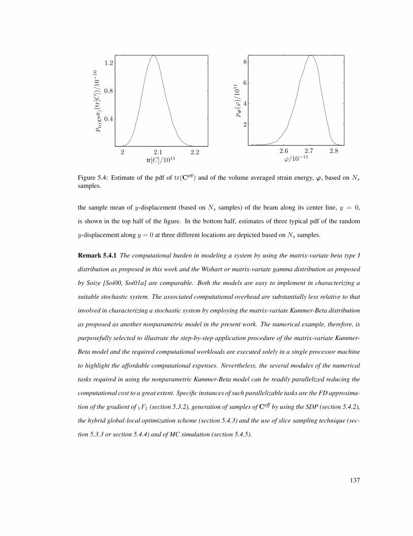
tr[C]/10112.1 2.2

ptr

(Cef

f )(t

r[C

])/10−

10

0.4

0.8

1.2

ϕ/10−112.6 2.7 2.8

2

2

4

6

8

pϕ(ϕ

)/1011

Figure 5.4: Estimate of the pdf of tr(Ceff) and of the volume averaged strain energy, ϕ, based on Ns

samples.

the sample mean of y-displacement (based on Ns samples) of the beam along its center line, y = 0,

is shown in the top half of the figure. In the bottom half, estimates of three typical pdf of the random

y-displacement along y = 0 at three different locations are depicted based on Ns samples.

Remark 5.4.1 The computational burden in modeling a system by using the matrix-variate beta type I

distribution as proposed in this work and the Wishart or matrix-variate gamma distribution as proposed

by Soize [Soi00, Soi01a] are comparable. Both the models are easy to implement in characterizing a

suitable stochastic system. The associated computational overhead are substantially less relative to that

involved in characterizing a stochastic system by employing the matrix-variate Kummer-Beta distribution

as proposed as another nonparametric model in the present work. The numerical example, therefore, is

purposefully selected to illustrate the step-by-step application procedure of the matrix-variate Kummer-

Beta model and the required computational workloads are executed solely in a single processor machine

to highlight the affordable computational expenses. Nevertheless, the several modules of the numerical

tasks required in using the nonparametric Kummer-Beta model can be readily parallelized reducing the

computational cost to a great extent. Specific instances of such parallelizable tasks are the FD approxima-

tion of the gradient of 1F1 (section 5.3.2), generation of samples of Ceff by using the SDP (section 5.4.2),

the hybrid global-local optimization scheme (section 5.4.3) and the use of slice sampling technique (sec-

tion 5.3.3 or section 5.4.4) and of MC simulation (section 5.4.5).

137

x (in m)

0.8889 8 16

Uy(x

)/10−

9(i

nm

)

−1

−2

−3

Uy(x = 0.8889)/10−9

−0.04 −0.01

pU

y(U

y)/

109

500

1000

Uy(x = 8)/10−9−1.2 −0.8

pU

y(U

y)/

109

00

0

10

20

Uy(x = 16)/10−9−3.6 −3.2

pU

y(U

y)/

109

2

4

6

Figure 5.5: Statistics of the random response of the cantilever beam; Uy(x) represents the random dis-

placement of the beam in y-direction along the center line of the beam, y = 0; E[Uy(x)] is the sample

mean of Uy(x) estimated based on Ns samples.

5.5 Conclusions

A MaxEnt based random matrix formalism is proposed in the present work to construct the probability

model of a stochastic mechanical structure whose system matrix, C, is symmetric positive definite and

strictly bounded from below and above in the positive definite sense by two deterministic symmetric pos-

itive definite matrices, Cl and Cu, as shown in (5.1). Two distinct distributions result from the MaxEnt

formulation depending on the information made use of in constructing the probability model of C. The

first probability model is the matrix-variate beta type I distribution that results from imposing two partic-

ular constraints in the MaxEnt framework guaranteeing negligible probability mass near the two bounds

thus taking care of the strict-bound conditions. The second probability model is the outcome of enforcing

the additional constraint of the mean matrix of C yielding the matrix-variate Kummer-Beta distribution.

The former probability model would be more useful if the “gap” between the two bounds, Cl and Cu,

138

is narrow so that imposing the mean matrix constraint is not essential. The later probability model, on

the other hand, would be particularly suitable if the “gap” between the two bounds are relatively wide

yielding higher level of scatter so that enforcing the mean matrix would be beneficial in capturing the

known first-order statistic of C.

While the proposed approach can be applied to characterize a broader spectrum of stochastic systems,

the motivation behind choosing the particular numerical example on homogenization of a heterogeneous

material is close in spirit with two recent works [SZ06, Soi08]. But it is also distinct in key respects

as explained next. One of these works [SZ06] relies on the higher-order statistics of the morphologi-

cal features of the experimental micrographs to characterize the random effective material property (e.g.,

Young’s modulus etc.) within the parametric framework. The corresponding bounds of the effective mate-

rial property are not used in constructing the associated probability model in that work but a finite set of

simulated samples are used to cross-check if the samples lie within the bounds. The present work, besides

being developed within a nonparametric framework, explicitly enforces the bounds in constructing the

pdf of Ceff. It also requires minimal information about the morphological features, or the experimentally

identified complete morphological features are precisely and implicitly incorporated into the bounds, Cl

andCu. The information about the morphological features are also embedded into the statistics such as cl,

cu andC while estimating them from the experimentally identified samples of Ceff. Minimal information

(i.e., volume fractions of the different phases of the heterogeneous material) is used if (5.8) is employed.

The experimentally identified complete morphological features, on the other hand, are inherently taken

into account while computing the bounds as well as cl, cu and C from the samples of Ceff by employ-

ing numerical analysis (e.g., FE technique) of the micrograph specimens. In such cases, the individual

material properties are appropriately assigned to the different phases and the resulting specimens are

subsequently subjected to SUBC, KUBC and computational tension test (or operational/representative

boundary conditions including a combination of traction or displacement boundary conditions depend-

ing on the test-setup) [Hue90, HH94]. Therefore, no attempt is made in the present work to explicitly

incorporate the higher-order statistics of the morphological features of the micrographs in characteriz-

ing the random effective material property. The other work [Soi08], published after the present work

was completed, is carried out within the nonparametric formulation but proposes to use the Wishart or

matrix-variate gamma distribution supported over M+N(R) thus violating the significant bound constraints

as indicated by (5.1).

139

The nonparametric homogenization scheme as proposed in section 5.4.2 is a much less time-

consuming technique both experimentally and computationally since it requires application of only one

boundary condition to extract the full matrix (samples of Ceff) simultaneously. The similar scheme, in

fact, can also be efficiently used in determining the lower and upper bounds, Cl, Cu ∈ M+N(R), of Ceff

when Cl and Cu are obtained by applying the SUBC and KUBC, instead of using the Reuss and Voigt

type bounds as used in the present work, in order to achieve slightly tighter bounds.

The present work also critically investigates the existing schemes for estimating the parameter, α,

of GN(α,ΛU ). A new scheme is proposed to estimate α if a set of samples of U ∼ GN(α,ΛU) are

available or a consistent value of ul in (5.24)M

+N(R) can be specified, which would be fundamentally more

congruous with the very basic motive of seeking a MaxEnt based pdf estimate.

140

Chapter 6

Current and Future Research Tasks

The greater danger for most of us is not that our aim is too high and we miss it,

but that it is too low and we reach it.

∼ Michelangelo di Lodovico Buonarroti Simoni (March 6, 1475 – February 18, 1564)

Based on the study carried out in this dissertation, the followings are a few ongoing works and sug-

gestions for future research plan:

1. (Chapter 2) While the asymptotic probability density function (apdf) of the estimators of the poly-

nomial chaos (PC) coefficients is identified as multivariate normal probability density function

(pdf), a careful reflection from consideration of the moment-based constraints would reveal that the

support of the estimators of the PC coefficients should be a proper subset of R(P+1). Thus, there is

a further need to investigate this issue along with the effect of truncation of the infinite-series based

PC expansion at a finite P <∞.

2. (Chapter 3) Identification of the appropriate apdf of the estimators of the PC coefficients based

on histogram could be another research topic since it would also be useful in determining the

confidence interval as discussed in the context of the work presented in chapter 2.

3. (Chapter 2–3) The constraint, nd = M , is required to be relaxed to identify an optimal functional

(PC) dimension of the random variate under investigation. A maximum-entropy (MaxEnt) based

procedure, with a goal to minimize the mean-square error (MSE) of the resulting PC expansion, has

recently been formulated but the associated algorithm still requires to be validated on a benchmark

problem.

4. (Chapter 4) A time-domain coupling technique for coupling the parametric and nonparametric sub-

systems has also recently been formulated. However, its potential applicability and computational

efficiency are yet to be tested.

141

5. (Chapter 5) A more efficient and robust algorithms, or reformulation of the optimization problem,

for computing the parameters of the matrix-variate Kummer-Beta distribution could be another

interesting topic. Special attentions are also due for more user friendly sampling schemes.

As a part of this task, one mathematical research topic could be to search for a closed-form expres-

sion for the differentiation of the confluent hypergeometric function of matrix argument with respect

to the elements of the associated matrix.

6. (Chapter 5) The proposed approach needs to be extended or/and applied to a several other signif-

icant practical problems including, but not limited to, microstructures with cracks (a simple semi-

definite programming (SDP) based algorithm has recently been formulated but yet to be tested

on practical data), marine structures subjected to underwater detonation (this would probably also

require coupling approach similar to the one presented in chapter 4), living cells, network systems

(e.g., transportation network system) etc.

7. (Chapter 4–Chapter 5) Incorporation of additional higher order statistics (for example, covariance

tensors) of the random matrix or/and mechanics-based constraints into the MaxEnt formulation

would also be a practically appealing research topic.

8. (Chapter 5) Extension of the (discretized) random matrix based approach to the case with contin-

uous stochastic operators would be another potential research task.

9. (Chapter 4-Chapter 5) Another interesting research topic would be to characterize a random vari-

ate by using orthogonal polynomials of matrix argument.

142

References

[ABC+97] J. R. Apel, B. Badiey, C. S. Chiu, S. Finette, J. Headrick, J. N. Kemp, J. F. Lynch,

A. Newhall, M. H. Orr, B. H. Pasewark, D. Tielbuerger, A. Turgut, K. von der Heydt,

and S. Wolf. An overview of the 1995 SWARM shallow-water internal wave acoustic

scattering experiment. IEEE Journal of Oceanic Engineering, 22(3):465–500, 1997.

[ACB08] M. Arnst, D. Clouteau, and M. Bonnet. Inversion of probabilistic structural models using

measured transfer functions. Computer Methods in Applied Mechanics and Engineering,

197(6-8):589–608, 2008.

[Adh07] Sondipon Adhikari. Matrix variate distributions for probabilistic structural dynamics. AIAA

Journal, 45(7):1748–1762, July 2007.

[And03] T.W. Anderson. An Introduction to Multivariate Statistical Analysis. Wiley-Interscience,

New Jersy, 2003.

[AS70] Milton Abramowitz and Irene A. Stegun. Handbook of Mathematical Functions: with

Formulas, Graphs, and Mathematical Tables. Dover Publications, Inc., New York, 1970.

[AS07] Y. Aoyagi and K. Shizawa. Multiscale crystal plasticity modeling based on geometrically

necessary crystal defects and simulation on fine-graining for polycrystal. International

Journal of Plasticity, 23(6):1022–1040, 2007.

[Bar33] M. S. Barlett. On the theory of statistical regression. Proceedings of the Royal Society of

Edinburgh, 53:260–283, 1933.

[Bar98] R.R. Barton. Simulation metamodels. In D.J. Medeiros, E.F. Watson, J.S. Carson, and

M.S. Manivannan, editors, Proceedings of the 1998 Winter Simulation Conference, 1998.

[BAS+06] A. Brahme, M. H. Alvi, D. Saylor, J. Fridy, and A. D. Rollett. 3D reconstruction of

microstructure in a commercial purity aluminum. Scripta Materialia, 55(1):75–80, July

2006.

[Baz00] Zdenek P. Bazant. Size effect. International Journal of Solids and Structures, 37(1-2):69–

80, 2000.

[Ber99] D. Bertsekas. Nonlinear Programming. Athena Scientific, Belmont, Massachusetts, USA,

1999.

[BLT03] I. Babuska, Kang-M. Liu, and R. Tempone. Solving stochastic partial differential equations

based on the experimental data. Mathematical Models and Methods in Applied Sciences,

13(3):415–444, 2003.

143

[BP04] Alain Bourgeat and Andrey Piatnitski. Approximations of effective coefficients in stochas-

tic homogenization. Annales de l’Institut Henri Poincare – Probabilites et Statisques,

40(2):153–165, 2004.

[BPP96] A.L. Berger, S.A.D. Pietra, and V.J.D. Pietra. A maximum entropy approach to natural

language processing. Comput. Linguist., 22(1):39–71, 1996.

[BTC79] A. Ben-Tal and A. Charnes. A dual optimization framework for some problems of infor-

mation theory and statistics. Problems of Control and Information Theory, 8:387–401,

1979.

[BTTC88] A. Ben-Tal, M. Teboulle, and A. Charnes. The role of duality in optimization problems

involving entropy functionals with applications to information theory. J. Optim. Theory.

Appl., 58(2):209–223, August 1988.

[BTZ05] I. Babuska, R. Tempone, and G.E. Zouraris. Solving elliptic boundary value problems with

uncertain coefficients by the finite element method: the stochastic formulation. Computer

Methods in Applied Mechanics and Engineering, 194(12-16):1251–1294, 2005.

[BW02] R.W. Butler and A.T.A Wood. Laplace approximation for hypergeometric functions with

matrix argument. The Annals of Statistics, 30(4):1155–1177, 2002.

[CB02] G. Casella and R.L. Berger. Statistical Inference. Duxbury, USA, 2002.

[CBS00] G. Christakos, P. Bogaert, and M. Serre. Temporal GIS: Advanced Functions for Field-

Based Applications. Springer, 2000.

[CF06] Wen Chen and Jacob Fish. A mathematical homogenization perspective of virial stress.

International Journal for Numerical Methods in Engineering, 67:189–207, 2006.

[CLPP+07] E. Capiez-Lernouta, M. Pellissetti, H. Pradlwarter, G. I. Schueller, and C. Soize. Data

and model uncertainties in complex aerospace engineering systems. Journal of Sound and

Vibration, 295(3-5):923–938, 2007.

[CLR96] G. Chryssolouris, M. Lee, and A. Ramsey. Confidence interval prediction for neural net-

works models. IEEE Transactions on Neural Networks, 7(1):229–232, January 1996.

[CM47] R.H. Cameron and W.T. Martin. The orthogonal development of non-linear functionals in

series of Fourier-Hermite functionals. Ann. Math. (2), 48(2):385–392, April 1947.

[CN97] M.C. Cario and B.L. Nelson. Modeling and generating random vectors with arbitrary

marginal distributions and correlation matrix. Technical report, Department of Industrial

Engineering and 35 Management Sciences, Northwestern University, Evanston, Illinois,

1997. http://citeseer.ist.psu.edu/cario97modeling.html.

[CR99] R.T. Clemen and T. Reilly. Correlations and copulas for decision and risk analysis. Man-

agement Science, 45(2):208–224, February 1999.

[Das07] Sonjoy Das. Efficient calculation of Fisher information matrix: Monte Carlo approach

using prior information. Master’s thesis, Department of Applied Mathematics and Statis-

tics, The Johns Hopkins University, Baltimore, Maryland, USA, May 2007. http:

//dspace.library.jhu.edu/handle/1774.2/32459.

[Dat05] Jon Dattorro. Convex Optimization & Euclidean Distance Geometry. Meboo Publishing

USA, 2005. Corrected version in 2007.

144

[DG04] Sonjoy Das and Roger Ghanem. Uncertainty analysis for surface ship subjected to under-

water detonation. In Proceedings of the IMAC-XXII Conference & Exposition on Structural

Dynamics, 26-29 January 2004.

[DGS06] C. Desceliers, R. Ghanem, and C. Soize. Maximum likelihood estimation of stochastic

chaos representation from experimental data. International Journal for Numerical Methods

in Engineering, 66(6):978–1001, 2006.

[DGS08] Sonjoy Das, Roger Ghanem, and James C. Spall. Asymptotic sampling distribution for

polynomial chaos representation of data : A maximum-entropy and Fisher information

approach. SIAM Journal on Scientific Computing, (accepted), 2008.

[DLRC05] O. Diard, S. Leclercq, G. Rousselier, and G. Cailletaud. Evaluation of finite element based

analysis of 3D multicrystalline aggregates plasticity: Application to crystal plasticity model

identification and the study of stress and strain fields near grain boundaries. International

Journal of Plasticity, 21(4):691–722, 2005.

[DM01] G. Deodatis and R.C. Micaletti. Simulation of highly skewed non-Gaussian stochastic

processes. Journal of Engineering Mechanics - ASCE, 127(12):1284–1295, December

2001.

[DM03] Sonjoy Das and C.S. Manohar. Prediction of vibration energy flow variability in random

built-up structures. In Proceedings of the 74th Shock and Vibration Symposium, 2003.

[DNM+03] B.J. Debusschere, H.N. Najm, A. Matta, O.M. Knio, R.G. Ghanem, and O.P. Le Maıtre.

Protein labeling reactions in electrochemical microchannel flow: Numerical simulation and

uncertainty propagation. Physics Of Fluids, 15(8):2238–2250, August 2003.

[DNP+04] B.J. Debusschere, H.N. Najm, P.P. Pebay, O.M. Knio, R. Ghanem, and O.P. Le Maıtre.

Numerical challenges in the use of polynomial chaos representations for stochastic pro-

cesses. SIAM J. Sci. Comput., 26(2):698–719, 2004.

[DOS06] X. Du and Martin Ostoja-Starzewski. On the scaling from statistical to representative

volume element in the thermoelasticity of random materials. Networks and heterogeneous

media, 1(2):259–274, June 2006.

[DSC04] C. Desceliers, C. Soize, and S. Cambier. Non-parametric-parametric model for random

uncertainties in non-linear structural dynamics: Application to earthquake engineering.

Earthquake Engineering and Structural Dynamics, 33(4):315–327, 2004.

[DSG07] C. Descelliers, C. Soize, and R. Ghanem. Identification of chaos representations of elastic

properties of random media using experimental vibration tests. Computational Mechanics,

39(6):831–838, 2007.

[DW96] W. J. Drugan and J. R. Willis. A micromechanics-based nonlocal constitutive equation

and estimates of representative volume element size for elastic composites. Journal of the

Mechanics and Physics of Solids, 44:497–524, 1996.

[DWR07] F. P. E. Dunne, A. Walker, and D. Rugg. A systematic study of hcp crystal orientation

and morphology effects in polycrystal deformation and fatigue. Proceedings of the Royal

Society of London. Series A, 463(2082):1467–1489, March 2007.

[EE03] W. E and B. Engquist. The heterogeneous multiscale methods. Communications in Math-

ematical Sciences, 1(1):87–133, 2003.

145

[EMS01] P. Embrechts, A.J. McNeil, and D. Straumann. Correlation and dependence in risk man-

agement: Properties and pitfalls. In M.A.H. Dempster, editor, Risk Management : Value at

Risk and Beyond, pages 176–223. Cambridge University Press, 2001.

[Fis96] G.S. Fishman. Monte Carlo: Concepts, Algorithms and Applications. Springer, New York,

1996.

[Fla89] H. Flanders. Differential Forms with Applications to the Physical Sciences. Dover Publi-

cations Inc., New York, 1989.

[FNS+07] Jacob Fish, Mohan A. Nuggehally, Mark S. Shephard, Catalin R. Picu, Santiago Badia,

Michael L. Parks, and Max Gunzburger. Concurrent AtC coupling based on a blend of the

continuum stress and the atomistic force. Computer Methods in Applied Mechanics and

Engineering, 196(45-48):4548–4560, 2007.

[For08] P. Forrester. Log-gases and Random matrices. Book in progress, 2008. http://www.ms.

unimelb.edu.au/˜matpjf/matpjf.html.

[FOT+00] S. Finette, M.H. Orr, A. Turgut, J.R. Apel, C.S. Badiey, B. Chiu, J. Headrick, J.N. Kemp,

J.F. Lynch, A.E. Newhall, K.von der Heydt, B.H. Pasewark, S.N. Wolf, and D. Tielbuerger.

Acoustic field variability induced by time evolving internal wave fields. Journal of the

Acoustical Society of America, 108(3):957–972, September 2000.

[FRT97] Shu-Cheng Fang, J.R. Rajasekera, and H.S.J. Tsao. Entropy Optimization, and Mathemat-

ical Programming. Kluwer Academic Publishers, Boston, USA, 1997.

[GD06] R. Ghanem and A. Doostan. On the construction and analysis of stochastic models: Char-

acterization and propagation of the errors associated with limited data. J. Comput. Phys.,

217(1):63–81, September 2006.

[GGG05] T. Gneiting, M.G. Genton, and P. Guttorp. Geostatistical space-time models, stationarity,

separability and full symmetry. Technical Report 475, Department of Statistics, University

of Washington, 2005. Also references therein. http://www.stat.washington.edu/

www/research/reports/2005/tr475.pdf.

[GGRH05] D. Ghosh, R. Ghanem, and J. Red-Horse. Analysis of eigenvalues and modal interaction

of stochastic systems. AIAA Journal, 43(10):2196–2201, October 2005.

[GH02] S. Ghosh and S.G. Henderson. Chessboard distributions and random vectors with speci-

fied marginals and covariance matrix. Operations Research, 50(5):820–834, September-

October 2002.

[GH03] S. Ghosh and S.G. Henderson. Behavior of the NORTA method for correlated random vec-

tor generation as the dimension increases. ACM Transactions on Modeling and Computer

Simulation, 13(3):276–294, July 2003. (for a short and conference version of the paper,

see http://www.informs-cs.org/wsc02papers/034.pdf).

[Gha99] R. Ghanem. Ingredients for a general purpose stochastic finite elements implementation.

Computer Methods in Applied Mechanics and Engineering, 168(1-4):19–34, 1999.

[GN00] A.K. Gupta and D.K. Nagar. Matrix Variate Distribution. Chapman & Hall/CRC, Boca

Raton, 2000.

[GRH99] R. Ghanem and J. Red-Horse. Propagation of uncertainty in complex physical systems

using a stochastic finite element approach. Phys. D, 133(1-4):137–144, 1999.

146

[Gri98] M. Grigoriu. Simulation of stationary non-Gaussian translation processes. Journal of

Engineering Mechanics - ASCE, 124(2):121–126, February 1998.

[GS91] R. Ghanem and P.D. Spanos. Stochastic Finite Elements: A Spectral Approach. Springer-

Verlag, New York, USA, 1991. Revised edition published by Dover Publications Inc. in

2003.

[GSD07] R. Ghanem, G. Saad, and A. Doostan. Efficient solution of stochastic systems: Application

to the embankment dam problem. Structural Safety, 29(3):238–251, 2007.

[Gus97] Andre1 A. Gusev. Representative volume element size for elastic composites : A numerical

study. Journal of the Mechanics and Physics of Solids, 45(9):1449–1459, 1997.

[Har97] D.A. Harville. Matrix Algebra from a Statistician’s Perspective. Springer, 1997.

[HD97] J.T.G. Hwang and A.A. Ding. Prediction intervals for artificial neural networks. Journal

of the American Statistical Association, 92(438):748–757, June 1997.

[HH94] S. Hazanov and C. Huet. Order relationship for boundary conditions effect in heterogonous

bodies smaller than the representative volume. Journal of the Mechanics and Physics of

Solids, 42(12):1995–2011, 1994.

[Hil63] R. Hill. Elastic properties of reinforced solids: Some theoretical principles. Journal of the

Mechanics and Physics of Solids, 11(5):357–372, 1963.

[HJ85] R.A. Horn and C.R. Johnson. Matrix Analysis. Cambridge University Press, 1985.

[HLD04] W. Hormann, J. Leydold, and G. Derflinger. Automatic Nonuniform Random Variate Gen-

eration. Springer, 2004.

[HM00] A. Haldar and S. Mahadevan. Reliability Assessment using Stochastic Finite Element Anal-

ysis. John Wiley & Sons, 2000.

[HS63] Z. Hashin and S. Shtrikman. A variational approach to the theory of the elastic behavior of

multiphase materials. Journal of the Mechanics and Physics of Solids, 11:127–140, 1963.

[Hue90] C. Huet. Application of variational concepts to size effects in elastic heterogenous bodies.

Journal of the Mechanics and Physics of Solids, 38(6):813–841, 1990.

[Ize91] A.J. Izenman. Recent developments in nonparametric density estimation. Journal of the

American Statistical Association, 86(413):205–224, March 1991.

[Jay57a] E.T. Jaynes. Information theory and statistical mechanics. Physical Review, 106(4):620–

630, May 1957.

[Jay57b] E.T. Jaynes. Information theory and statistical mechanics. Physical Review, 108(2):171–

197, October 1957.

[Jay68] E.T. Jaynes. Prior probabilities. IEEE Transactions on Systems and Cybernetics, SSC-

4(3):227–241, 1968.

[JBF88] B. Jetmundsen, R.L. Bielawa, and W.G. Flannelly. Generalized frequency domain sub-

structure synthesis. Journal of the American Helicopter Society, 33(1):55–64, 1988.

[Jef46] H. Jeffreys. An invariant form for the prior probability in estimation problems. Pro-

ceedings of the Royal Society of London. Series A, Mathematical and Physical Sciences,

186(1007):453–461, September 1946.

147

[Joe97] H. Joe. Multivariate Models and Dependence Concepts. Chapman & Hall, 1997.

[Jol02] I.T. Jolliffe. Principal Component Analysis. Springer, 2nd edition, October 2002.

[Kap89] J.N. Kapur. Maximum Entropy Models in Science and Engineering. Wiley Eastern Limited,

India, 1989. Revised edition in 1993.

[KC06] D. Kurowicka and R. Cooke. Uncertainty Analysis with High Dimensional Dependence

Modelling. John Wiley & Sons Ltd, 2006.

[KE06] P. Koev and A. Edelman. The efficient evaluation of the hypergeometric function of a

matrix argument. Mathematics and Computation, 75(254):833–846, 2006.

[KFG+03] T. Kanit, S. Forest, I. Galliet, V. Mounoury, and D. Jeulin. Determination of the size of the

representative volume element for random composites: statistical and numerical approach.

International Journal of Solids and Structures, 40(13-14):3647–3679, 2003.

[KGB02] V. Kouznetsova, M. G. D. Geers, and W. A. M. Brekelmans. Multi-scale constitutive mod-

elling of heterogeneous materials with a gradient-enhanced computational homogenization

scheme. International Journal for Numerical Methods in Engineering, 54(8):1235–1260,

2002.

[KGB04] V. Kouznetsova, M. G. D. Geers, and W. A. M. Brekelmans. Size of a representative vol-

ume element in a second-order computational homogenization framework. International

Journal for Multiscale Computational Engineering, 2(4):575–598, 2004.

[KGL04] Kai Kadau, Timothy C. Germann, and Peter S. Lomdahl. Large-scale molecular-dynamics

simulation of 19 billion particles. International Journal of Modern Physics C, 15(1):193–

201, 2004. Also see http://www.lanl.gov/orgs/t/publications/research_

highlights_2005/docs/SF05_Kadau_WorldRecord.pdf.

[Kha70] C. G. Khatri. A note on Mitra’s paper “A density-free approach to the matrix variate beta

distribution”. Sankhaya: Series A, 32:311–318, 1970.

[KK92] J.N. Kapur and H.K. Kesavan. Entropy Optimization Principles with Applications. Aca-

demic Press Inc., Boston, USA, 1992.

[KL51] S. Kullback and R.A. Leibler. On information and sufficiency. The Annals of Mathematical

Statistics, 22(1):79–86, March 1951.

[KPU04] Y. Kouskoulas, L.E. Pierce, and F.W. Ulaby. A computationally efficient multivariate

maximum-entropy density estimation (MEDE) technique. IEEE Transactions on Geo-

science and Remote Sensing, 42(2):457–468, February 2004.

[KTH92] M. Kleiber, D.H. Tran, and T.D. Hien. The Stochastic Finite Element Method. John Wiley

& Sons, 1992.

[Kul59] S. Kullback. Information Theory and Statistics. John Wiley & Sons, New York, 1959.

Republished by Dover Publications Inc. in 1997.

[Lan57] H.O. Lancaster. Some properties of the bivariate normal distribution considered in the form

of a contingency table. Biometrika, 44(1-2):289–292, June 1957.

[Leb72] N.N. Lebedev. Special Functions and Their Applications. Dover Publications, New York,

1972.

148

[Leh75] E.L. Lehmann. Nonparametrics: Statistical methods based on ranks. McGraw-Hill Inter-

national Book Company, New York, 1975.

[Lin88] B.G. Lindsay. Composite likelihood methods. Contemporary Mathematics, 80:221–239,

1988.

[Liu00] W. Liu. Structural Dynamic Analysis and Testing of Coupled Structures. PhD thesis,

Department of Mechanical Engineering, Imperial College of Science, Technology and

Medicine, University of London, October 2000.

[LKP06] Wing Kam Liu, Eduard G. Karpov, and Harlod S. Park. Nano Mechanics and Materials:

Theory, Multiscale Methods and Applications. John Wiley & Sons, Ltd., 2006.

[LL04] C.Q. Liu and X. Liu. A new method for analysis of complex structures based on FRF’s of

substructures. Shock and Vibration, 11(1):1–7, 2004.

[LLY99] Ju Li, Dongyi Liao, and Sidney Yip. Nearly exact solution for coupled continuum/MD

fluid simulation. Journal of Computer-Aided Materials Design, 6:95–102, 1999.

[LMNGK04] O.P. Le Maıtre, H. Najm, R. Ghanem, and O. Knio. Multi-resolution analysis of Wiener-

type uncertainty propagation schemes. J. Comput. Phys., 197(2):502–531, 2004.

[LMNP+07] O.P. Le Maıtre, H. Najm, P.P. Pebay, R.G. Ghanem, and O.M. Knio. Multi-resolution-

analysis scheme for uncertainty quantification in chemical systems. SIAM J. Sci. Comput.,

29(2):864889, 2007.

[Loe78] M. Loeve. Probability Theory II. Springer-Verlag, New York, 1978.

[Lof04] J. Lofberg. YALMIP: A toolbox for modeling and optimization in MATLAB. In Proceed-

ings of the IEEE Conference on Computer Aided Control Systems Design (CACSD), Taipei,

Taiwan, 2004. http://control.ee.ethz.ch/˜joloef/yalmip.php.

[Man01] P.S. Mann. Introductory Statistics. John Wiley & and Sons, 4th edition, 2001.

[Mat97] A.M. Mathai. Jacobians of Matrix Transformations and Functions of Matrix Argument.

World Scientific, 1997.

[MB93] A.M.H. Meeuwissen and T. Bedford. Probability distributions with given marginals and

given correlation that have maximal entropy. Technical Report 93-81, Department of Tech-

nical Mathematics and Informatics, Delft University of Technology, Delft, The Nether-

lands, 1993.

[MB97] A.M.H. Meeuwissen and T. Bedford. Minimally informative distributions with given rank

correlation for use in uncertainty analysis. Journal of Statistical Computation and Simula-

tion, 57(1-4):143–174, 1997.

[Meh04] M.L. Mehta. Random Matrices. Academic Press, 3rd edition, 2004.

[MI99] C.S. Manohar and R.A. Ibrahim. Progress in structural dynamics with stochastic parameter

variations: 1987-98. Applied Mechanical Reviews, 52(5):177–197, 1999. also references

therein.

[Mit70] S. K. Mitra. A density-free approach to the matrix variate beta distribution. Sankhaya:

Series A, 32:81–88, 1970.

[Mur82] R.J. Murihead. Aspects of Multivariate Statistical Theory. John Wiley & Sons Inc., 1982.

Revised printing in 2005.

149

[MVL06] Cahal McVeigh, Franck Vernerey, and Brinson L. Cate Liu, Wing Kam. Multiresolution

analysis for material design. Computer Methods in Applied Mechanics and Engineering,

195:5053–5076, 2006.

[Nea03] Radford M. Neal. Slice sampling. The Annals of Statistics, 31(3):705–741, June 2003.

with discussions.

[Nel06] R.B. Nelsen. An Introduction to Copulas. Springer, 2006.

[NG02] D.K. Nagar and A.K. Gupta. Matrix-variate Kummer-Beta distribution. Journal of the

Australian Mathematical Society, 73:11–25, 2002.

[NNH99] Sia Nemat-Nasser and Muneo Hori. Micromechanics: Overall properties of heterogeneous

materials. Elsevier, Amsterdam, 2nd revised edition, 1999.

[OS01] Martin Ostoja-Starzewski. Mechanics of random materials: Stochastics, scale effects and

computation. In Dominique Jeulin and Martin Ostoja-Starzewski, editors, Mechanics of

Random and Multiscale Microstructures, pages 93–161. Springer-Verlag, 2001.

[OS02] Martin Ostoja-Starzewski. Microstructural randomness versus representative volume ele-

ment in thermodynamics. Journal of Applied Mechanics, 69(1):25–35, January 2002.

[OS08] Martin Ostoja-Starzewski. Microstructural Randomness and Scaling in Mechanics of

Materials. Chapman & Hall/CRC, 2008.

[OSDKL07] M. Ostoja-Starzewski, X. Du, Z.F. Khisaeva, and W. Li. Comparisons of the size of

the representative volume element in elastic, plastic, thermoelastic, and permeable ran-

dom microstructures. International Journal for Multiscale Computational Engineering,

5(2):73–82, 2007.

[PB06] C. L. Pettit and P. S. Beran. Spectral and multiresolution Wiener expansions of oscillatory

stochastic processes. Journal of Sound and Vibration, 294:752–779, 2006.

[PG00] M.F. Pellissetti and R.G. Ghanem. Iterative solution of systems of linear equations arising

in the context of stochastic finite elements. Advances in Engineering Software, 31:607–

616, 2000.

[PG04] M. Pellissetti and R. Ghanem. A method for validation of the predictive computations using

a stochastic approach. Journal of Offshore Mechanics and Arctic Engineering, 126:227–

234, August 2004.

[Phi03] G.M. Phillips. Interpolation and Approximation by Polynomials. Springer, 2003.

[PPS02] B. Puig, F. Poirion, and C. Soize. Non-Gaussian simulation using Hermite polyno-

mial expansion: convergences and algorithms. Probabilistic Engineering Mechanics,

17(3):253–264, 2002.

[PQH04] K.K. Phoon, S.T. Quek, and H. Huang. Simulation of non-Gaussian process using fractile

correlation. Probabilistic Engineering Mechanics, 19:287–292, 2004.

[PTVF96] W.H. Press, S.A. Teukolsky, W.T. Vetterling, and B.P. Flannery. Numerical Recipes in

FORTRAN: The Art of Scientific Computing. Cambridge University Press, 1996.

[RB95] Y. Ren and C.F. Beards. On substructure synthesis with FRF data. Journal of Sound and

Vibration, 185(5):845–866, 1995.

150

[RDD07] D. Rugg, M. Dixon, and F. P. E. Dunne. Effective structural unit size in titanium alloys.

The Journal of Strain Analysis for Engineering Design, 42(4):269–279, 2007.

[RKL+02] Cindy L. Rountree, Rajiv K. Kalia, Elefterios Lidorikis, Aiichiro Nakano, Laurent Van

Brutzel, and Priya Vashishta. Atomistic aspects of crack propagation in brittle materials:

Multimillion atom molecular dynamics simulations. Annual Review of Materials Research,

32:377–400, 2002.

[RNGK03] M.T. Reagan, H.N. Najm, R.G. Ghanem, and O.M. Knio. Uncertainty quantification

in reacting-flow simulations through non-intrusive spectral projection. Combustion And

Flame, 132(3):545–555, February 2003.

[Ros52] M. Rosenblatt. Remarks on multivariate transformation. The Annals of Mathematical

Statistics, 23(3):470–472, September 1952.

[RZ04] Z.-Y. Ren and Q.-S. Zheng. Effect of grain sizes, shapes, and distribution on minimum

sizes of representative volume elements of cubic polycrysrals. Mechanics of Materials,

36:1217–1229, 2004.

[Sco92] D.W. Scott. Multivariate Density Estimation: Theory, Practice and Visualization. Wiley-

Interscience, August 1992.

[SFED+04] David M. Saylor, Joseph Fridy, Bassem S. El-Dasher, Kee-Young Jung, and Anthony D.

Rollett. Statistically representative three-dimensional microstructures based on orthogonal

observation sections. Metallurgical and Materials Transactions A — Physical Metallurgy

and Materials Science, 35A(7):1969–1979, July 2004.

[SG02a] S. Sakamoto and R. Ghanem. Polynomial chaos decomposition for the simulation of non-

gaussian nonstationary stochastic processes. Journal of Engineering Mechanics - ASCE,

128(2):190–201, February 2002.

[SG02b] S. Sakamoto and R. Ghanem. Simulation of multi-dimensional non-Gaussian non-

stationary random fields. Probabilistic Engineering Mechanics, 17(2):167–176, April

2002.

[SG04a] C. Soize and R. Ghanem. Physical systems with random uncertainties: Chaos representa-

tions with arbitrary probability measure. SIAM J. Sci. Comput., 26(2):395–410, 2004.

[SG04b] Shriram Swaminathan and Somnath Ghosh. Statistically equivalent representative volume

elements for unidirectional composite microstructures: Part ii — with interfacial debond-

ing. Journal of Composite Materials, 40(7):605–621, 2004.

[SGP04] Shriram Swaminathan, Somnath Ghosh, and N. J. Pagano. Statistically equivalent repre-

sentative volume elements for unidirectional composite microstructures: Part i - without

damage. Journal of Composite Materials, 40(7):583–604, 2004.

[Sha48] C.E. Shannon. A mathematical theory of communication. Bell System Technical Journal,

27(3,4):379–423, 623–656, July, October 1948.

[SJ80] J.E. Shore and R.W. Johnson. Axiomatic derivation of the principle of maximum entropy

and the principle of minimum cross-entropy. IEEE Transactions on Information Theory,

IT-26(1):26–37, January 1980.

[SJ83] J.E. Shore and R.W. Johnson. Comments on and correction to “axiomatic derivation of

the principle of maximum entropy and the principle of minimum cross-entropy”. IEEE

Transactions on Information Theory, IT-29(6):942–943, 1983.

151

[SK79] M. S. Srivastava and C. G. Khatri. An Introduction to Multivariate Statistics. North Hol-

land, New York, 1979.

[SK97] K. Shankar and A.J. Keane. Vibrational energy flow analysis using a substructure approach:

The application of receptance theory to fea and sea. Journal of Sound and Vibration,

201(4):491–513, 1997.

[SKR00] M. Srikanth, H.K. Kesavan, and P.H. Roe. Probability density function estimation using

the minmax measure. IEEE Transactions on Systems, Man, and Cybernatics - Part C:

Applications and Reviews, 30(1):77–83, February 2000.

[Soi99] C. Soize. A nonparametric model of random uncertainties in linear structural dynamics.

Publications du LMA-CNRS, ISBN 2-909669-16-5, 152:109–138, 1999.

[Soi00] C. Soize. A nonparametric model of random uncertainties for reduced matrix models in

structural dynamics. Probabilistic Engineering Mechanics, 15:277–294, 2000.

[Soi01a] C. Soize. Maximum entropy approach for modeling random uncertainties in transient elas-

todynamics. Journal of the Acoustical Society of America, 109(5):1979–1996, 2001. Pt. 1.

[Soi01b] C. Soize. Transient responses of dynamical systems with random uncertainties. Proba-

bilistic Engineering Mechanics, 16:363–372, 2001.

[Soi03] C. Soize. Random matrix theory and non-parametric model of random uncertainties in

vibration analysis. Journal of Sound and Vibration, 263:893–916, 2003.

[Soi05a] C. Soize. A comprehensive overview of non-parametric probabilistic approach of model

uncertainties for predictive models in structural dynamics. Journal of Sound and Vibration,

288:623–652, 2005.

[Soi05b] C. Soize. Random matrix theory for modeling uncertainties in computational mechanics.

Computer Methods in Applied Mechanics and Engineering, 194:1333–1366, 2005.

[Soi06] C. Soize. Non-Gaussian positive-definite matrix-valued random fields for elliptic stochastic

partial differential operators. Computer Methods in Applied Mechanics and Engineering,

195:26–64, 2006.

[Soi08] C. Soize. Tensor-valued random fields for meso-scale stochastic model of anisotropic elas-

tic microstructure and probabilistic analysis of representative volume element size. Proba-

bilistic Engineering Mechanics, (in press) doi:10.1016/j.probengmech.2007.12.019, 2008.

[Spa92] J. C. Spall. Multivariate stochastic approximation using a simultaneous perturbation gra-

dient approximation. IEEE Trans. Automat. Control, 37(3):332–341, 1992.

[Spa03] J. C. Spall. Introduction to Stochastic Search and Optimization: Estimation, Simulation

and Control. Wiley-Interscience, 2003.

[Spe04] C. Spearman. The proof and measurement of association between two things. The Ameri-

can Journal of Psychology, 15(1):72–101, January 1904.

[SZ06] Sethuraman Sankaran and Nicholas Zabaras. A maximum entropy approach for property

prediction of random microstructures. Acta Materialia, 54:2265–2276, 2006.

[Tol62] G.P. Tolstov. Fourier Series. Prentice-Hall, 1962.

[Tor02] Salvatore Torquato. Ranom Heterogeneous Materials: Microstructure and Macroscopic

Properties. Springer, 2002.

152

[TPO00] E.B. Tadmor, R. Phillips, and M. Ortiz. Hierarchical modeling in the mechanics of materi-

als. International Journal of Solids and Structures, 37(1-2):379–389, 2000.

[TV04] A.M. Tulino and S. Verdu. Random Matrix Theory and Wireless Communications. now

Publishers Inc., 2004.

[Urg91] A.P.V. Urgueira. Using the s.v.d. for the selection of independent connection coordinates

in the coupling of substructures. In Proceedings of the 9th International Modal Analysis

Conference, pages 919–925, 1991.

[VB96] Lieven Vandenberghe and Stephen Boyd. Semidefinite programming. SIAM Review,

38(1):49–95, March 1996.

[vdG98] P.A.G. van der Geest. An algorithm to generate samples of multi-variate distributions with

correlated marginals. Computational Statistics & Data Analysis, 27(3):271–289, 1998.

[VG08] Ashkan Vaziri and Arvind Gopinath. Cell and biomolecular mechanics in silico. Nature

Materials, 7(1):15–23, January 2008.

[Wie38] N. Wiener. The homogeneous chaos. Amer. J. Math., 60(4):897–936, 1938.

[WSB07] J.A.S. Witteveen, S. Sarkar, and H. Bijl. Modeling physical uncertainties in dynamic stall

induced fluidstructure interaction of turbine blades using arbitrary polynomial chaos. Com-

puters and Structures, 85(11-14):866–878, June-July 2007.

[Wu03] X. Wu. Calculation of maximum entropy densities with application to income distribution.

J. Econometrics, 115:347–354, 2003.

[XK02] D. Xiu and G.E. Karniadakis. The Wiener-Askey polynomial chaos for stochastic differ-

ential equations. SIAM J. Sci. Comput., 24(2):619–644, 2002.

[XLSK02] D. Xiu, D. Lucor, C.-H. Su, and G.E. Karniadakis. Stochastic modeling of flow-structure

interactions using generalized polynomial chaos. Journal of Fluids Engineering, 124:51–

59, March 2002.

[ZG04] Yu Zou and Roger Ghanem. A multiscale data assimilation with the ensemble Kalman

filter. Multiscale Modeling & Simulation, 3(1):131–150, 2004.

[ZKG05] Yu Zou, Ioannis Kevrekidis, and Roger Ghanem. Equation-free dynamic renormalization:

Self-similarity in multidimensional particle system dynamics. Physical Review E, 72:940–

956, 2005.

[Zv01] J. Zeman and M. Sejnoha. Numerical evaluation of effective elastic properties of graphite

fiber tow impregnated by polymer matrix. Journal of the Mechanics and Physics of Solids,

49:69–90, 2001.

[Zv07] J. Zeman and M. Sejnoha. From random microstructures to representative volume ele-

ments. Modelling and Simulation in Materials Science and Engineering, 15:S325–S335,

2007.

153

Appendices

154

Appendix A

Computation of PC Coefficients

This appendix describes an 1-dimensional (D) scheme based on interpolation technique. It would be

useful for the efficient computation of

1. {aj(y2)}j∈N in (3.7), or

2. {cj}j∈N in (3.12), or

3. {cjk}j∈N for any given k ∈ {1, · · · , N} in (3.15).

Since all these cases are similar, only the last case involving {cjk}j∈N, k ∈ {1, · · · , N}, would be

demonstrated below. Any other case can be readily tackled by considering the appropriate PC coefficients

and the PDFs.

Let the pdf and support of yk be denoted, respectively, by pykand sk = [lk, mk] ⊂ R. The com-

putation of cjk in (3.16) based on qk ≡ P−1ykPξk

needs solving an integral equation. For some given

ξk, the integral equation, Pξk(ξk) =

∫ yk

lkpyk

(y)dy, is to be solved for yk. Solving this integral equation

several times within the numerical integration algorithm, that is employed to compute cjk, significantly

increases the computational burden, and might also lead to certain numerical instability. To overcome

these difficulties and to increase the computational expediency and efficiency, a surrogate function, qk,

determined based on 1-D interpolation scheme, is used for qk in (3.16) to compute the PC coefficients,

cjk . The approximate function, qk, needs to be determined only once ∀j ∈ N.

Consider uk ≡ Pξk(ξk)

d= Pyk

(yk) (uk here should not be confused with the components of U in

sections 3.2.2–3.2.2). For a given yk ∈ syk= [lk, mk], finding uk as uk = Pyk

(yk) is, in general, much

cheaper than finding yk as yk = P−1yk

(uk) for a given uk ∈ [0, 1].

For each k ∈ {1, · · · , N}, let the support, sk, be divided equally into nk ∈ N intervals. Then,

the coordinates of the points defining these intervals are given by y(j)k = lk + j[(mk − lk)/nk], j =

0, · · · , nk. For each of these points, first compute u(j)k as u

(j)k = Pyk

(y(j)k ), and then compute ξ

(j)k as

ξ(j)k = P−1

ξk(u

(j)k ). Since Pξk

’s are suitably chosen standard measures associated with the commonly

155

used PC random variables, computation of P−1ξk

via closed form expression or efficient algorithms is

available in the statistical literature (see e.g., [Fis96, Section 3.2], [HLD04, Section 2.1]). As already

indicated, the statistical toolbox of MATLAB provides functions to evaluate the inverse of PDF for many

such standard PC random variables. Since Pykand Pξk

are monotonically increasing function, the set

of values in {ξ(j)k }nk

j=0 would be in the increasing order, ξ(0)k < · · · < ξ

(nk)k . The set, {ξ(j)k , y

(j)k }nk

j=0,

thus determined is now used to construct the approximate function, sξk∋ ξk 7−→ qk(ξk) ∈ syk

, by using

standard interpolation technique (see e.g., [Phi03, Chapter 1], [PTVF96, Chapter 3]). The basic MATLAB

package offers a function, interp1, use of which should be sufficient enough for determining qk for

many practical purposes. The approximate function, qk, is used as a proxy for qk in (3.16) to compute the

PC coefficients, cjk’s.

The error in approximating qk(ξk) by the resulting PC representation, q(Kk)k (ξk) =

∑Kk

j=0 cjk Ψj(ξk), for some large Kk ∈ N, is bounded above by the following relation,

|qk(ξk) − q(Kk)k (ξk) | ≤ |qk(ξk) − qk(ξk) |

+ | qk(ξk) − q(Kk)k (ξk) | a.s. (A.1)

The second error term is bounded above by some eKk(ξk) satisfying limKk→∞ eKk

(ξk) = 0 [Leb72,

Chapter 4] a.s. When a linear interpolation scheme is employed, the interpolated function, qk, is piecewise

linear in ξk and the first error term is then bounded above by O(h2k), in which hk = max1≤i≤nk

(ξ(i)k −

ξ(i−1)k ), [Phi03, Example 1.1.4] a.s. In establishing this error bound, O(h2

k), it is necessary for the

second derivative of qk to be piecewise bounded by some finite K, i.e., | ∂2qk(ξk)/∂ξk |≤ K on sξk

except possibly a finite number of points. As it is already mentioned that an assumption of piecewise

smoothness is required to arrive at the PC representation in a.s. sense, the piecewise linear function, qk,

that is actually being represented by PC formalism, automatically satisfies the assumption of piecewise

smoothness. Therefore, in order to satisfy (A.1), the assumption of piecewise smoothness of the original

function, qk, needs to be replaced by a relatively stronger assumption of the piecewise boundedness of

the second derivative of the function, qk.

156