TECHNIQUE FOR SOLVING SECOND ORDER

PARTIAL DIFFERENTIAL EQUATION FOR GROUND WATER CONTAMINANT FLOW MODEL

BY

UJILE, A.A*; ABOWEI, M. F. N. AND PUYATE, Y. T.

Department of Chemical/ Petrochemical Engineering Faculty of Engineering, Rivers State University of

Science & Technology, P M B 5080, Port Harcourt, Nigeria

ABSTRACT A solution procedure of the developed model equation, which describes the groundwater flow and solute transport, was carried out. Numerical method, which incorporates the Taylor Theorem using grid system in conjunction with analytical Euler methods, was applied to solve the partial differential model equations in two-dimensional flows. The solution of the final model equation is:

In o

A

C

C = In

h

MKdK bL )/ 1( –

tKh

MKdK dbbL .)/ 1( )/ 1(

Applications of the model in certain location (Yenagoa) in the Niger Delta Region, Nigeria show that the solution is unconditionally convergent and stable. The solution can be used to simulate both confined and unconfined flow and transport problems. 1.0 Introduction:

Contaminated water flows into the ground from the surface of the earth through pores in the soil and underlying geologic structure. Although these pores are very small and so account for only a small portion of the underground volume, contaminated water moves very slowly underground and can cover large distances in depth.1 Many researchers have studied the problem of solute movement through saturated porous media both analytically and numerically. However, published literature related to a field problem on a regional scale such as the present one, (Niger Delta region) is scarce. For example, Mercer2 modeled groundwater flow at Love canal; Bredehoeft and Pinder3 modeled the distribution of contaminant in an aquifer of glacial sediments; solute transport in limestone aquifer by Schwartz4; and assessment of salt water encroachment phenomenon by Ashim and Yapa5. * Corresponding Author

2

Of all the investigations carried out by other researchers there has not been any that considered regional assessment with the application of second order differential equations. This work involves not only solute transport and flow-model in a regional scale, but also multiple solute contaminants (Iron, chloride, hardness, salinity concentration levels) in the region with the application of second order differential equations. Abraham6 used a single cell model to study the regional chloride and nitrate pollution pattern in part of the coastal aquifer in Israel. Spanoudaki et al7 used the finite difference and orthogonal grids for Integrated Surface water-Groundwater modeling; Shahld and Rahman8 applied a two-dimensional groundwater flow for the delineation of wellhead protection area around water well and Fatta et al9 carried out numerical simulation of flow and contaminant migration at a municipal landfill. Park et al10 applied transport modeling to the interpretation of groundwater tracer. Other researchers have recently applied analytical method for the mass transfer coefficient and concentration boundary layer thickness for dissolving non-aqueous phase liquid pool in porous media. The solutions to second order partial differential equations given by other researchers contain other complex functions like Bessel functions, complementary errors functions, Hantush Well functions and others. These have created difficulties for graduate students and researchers for numerical/ analytical evaluations of parameters in practice. The dirac operators and non compact surfaces by Stefan and Hermann11 have posed complex conditions for researchers and graduates to solve partial differential equations. From the standpoint of the above, it becomes imperative to establish solutions to second order partial differential equation that will be simple to all practitioners and researchers. This work considers the existing difficulty and establishes solutions that contain only exponential function which is simple that hand calculator can solve. 2.0 Derivation Procedure: Considering the movement of the contaminated fluid from a solid waste landfill into potable water aquifer located beneath it, is an example of unwanted groundwater flow. The motion of fluid through porous rock induced by pressure and gravity forces is of great practical importance.

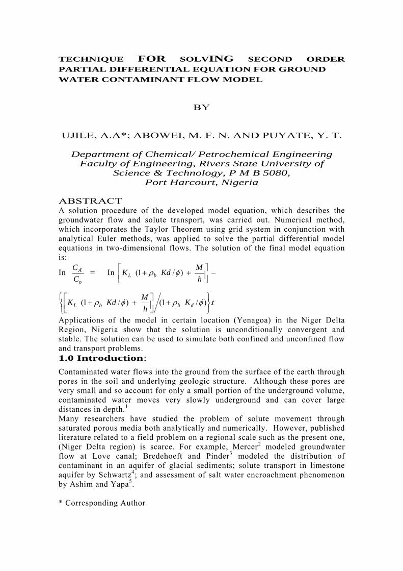
Taking the material balance on the leaching process in figure 1 in the x, y and z directions (UJILE, 2003) obtained the following expressions:

Fig.1 Plume behaviour of TCE (trichloro-ethylene) after 3.5 years NRC12

3

0.1........................

2

KCt

CR

z

CV

z

CD

zy

CVy

y

CDy

yx

CV

x

CD

x zi

xx

Taking the material balance on the leaching process in figure 1 in the x, y and z directions Ujile13 obtained the expressions shown in equation 1.0

Considering the plume of (trichloro-ethylene) TCE leachate figure 1 the direction of flow in horizontal x and vertical y directions is larger than the transverse z direction. The field data obtained from the Niger Delta region shows variation in hydraulic conductivity in different directions

i.e x

c

> y

c

>>> z

c

hence z

c

= 0, Vx > Vy >>> Vz; Vz 0

Then equation 1.0 becomes:

x

c

(Dx x

c

) – Vx x

c

+ y

c

(Dy y

c

) – Vy y

c

= R t

c

+ KC ….. 1.1

Equation 1.1 can be modified to the form.

2

2

2

2

y

CD

x

CD yx –

y

CV

x

CV yx = R

t

C

+ KC …... 1.2

2.1 Basic Engineering Assumptions: Movement of the solute is assumed to be in the plane of the horizontal and vertical section of the aquifer and the porous medium is assumed to be anisotropic with respect to the dispersivity of the medium. The density and viscosity of groundwater is assumed to be constant. This is the case in most ground water flow system. The groundwater flow pattern is not altered by the presence of multiple contaminants in solution. Aquifers with unconsolidated formation of sand and gravel are predominant in Niger Delta region, porosity is considered more or less uniform on a regional basis. (Range 0.33-0.45) The first order decay rate in liquid phase is the same as in soil (solid) phase, (i.e. KL = KS) The mass transfer coefficient of pollutant is considered on a macroscopic scale. This is because of hydraulic conductivity and porosity, which create

4

irregularities in the seepage velocity and consequently additional mixing of the pollutant.

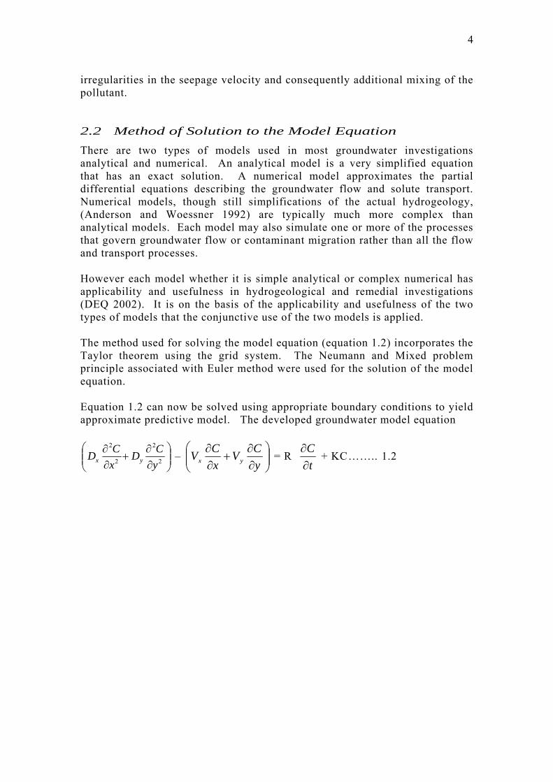
2.2 Method of Solution to the Model Equation

There are two types of models used in most groundwater investigations analytical and numerical. An analytical model is a very simplified equation that has an exact solution. A numerical model approximates the partial differential equations describing the groundwater flow and solute transport. Numerical models, though still simplifications of the actual hydrogeology, (Anderson and Woessner 1992) are typically much more complex than analytical models. Each model may also simulate one or more of the processes that govern groundwater flow or contaminant migration rather than all the flow and transport processes. However each model whether it is simple analytical or complex numerical has applicability and usefulness in hydrogeological and remedial investigations (DEQ 2002). It is on the basis of the applicability and usefulness of the two types of models that the conjunctive use of the two models is applied. The method used for solving the model equation (equation 1.2) incorporates the Taylor theorem using the grid system. The Neumann and Mixed problem principle associated with Euler method were used for the solution of the model equation. Equation 1.2 can now be solved using appropriate boundary conditions to yield approximate predictive model. The developed groundwater model equation

2

2

2

2

y

CD

x

CD yx –

y

CV

x

CV yx = R

t

C

+ KC …….. 1.2

5

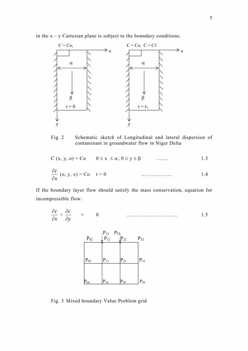
in the x – y Cartesian plane is subject to the boundary conditions.

Fig. 2 Schematic sketch of Longitudinal and lateral dispersion of contaminant in groundwater flow in Niger Delta

C (x, y, o) = Co 0 x ; 0 y ……. 1.3

x

c

(o, y, x) = Co t > 0 ……………… 1.4

If the boundary layer flow should satisfy the mass conservation, equation for

incompressible flow:

x

c

+ y

c

= 0 ………………………… 1.5

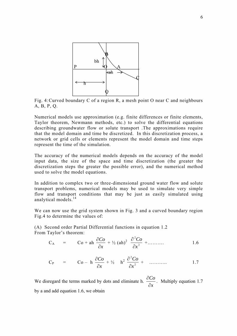
Fig. 3 Mixed boundary Value Problem grid

P13 P23 P02 P12 P22 P32

P01 P11 P21 P31

P00 P10 P20 P30

C = Co, x

t = 0

y

C = Co, C = C1 x

t = t1

y

6

Fig. 4: Curved boundary C of a region R, a mesh point O near C and neighbours A, B, P, Q. Numerical models use approximation (e.g. finite differences or finite elements, Taylor theorem, Newmann methods, etc.) to solve the differential equations describing groundwater flow or solute transport .The approximations require that the model domain and time be discretized. In this discretization process, a network or grid cells or elements represent the model domain and time steps represent the time of the simulation. The accuracy of the numerical models depends on the accuracy of the model input data, the size of the space and time discretization (the greater the discretization steps the greater the possible error), and the numerical method used to solve the model equations. In addition to complex two or three-dimensional ground water flow and solute transport problems, numerical models may be used to simulate very simple flow and transport conditions that may be just as easily simulated using analytical models.14 We can now use the grid system shown in Fig. 3 and a curved boundary region Fig.4 to determine the values of: (A) Second order Partial Differential functions in equation 1.2 From Taylor’s theorem:

CA = Co + ah x

Co

+ ½ (ah)2 2

2

x

Co

+………. 1.6

CP = Co – h x

Co

+ ½ h2 2

2

x

Co

+ ……….. 1.7

We disregard the terms marked by dots and eliminate h. x

Co

. Multiply equation 1.7

by a and add equation 1.6, we obtain

B

bh P O A

ah C h

Q

7

CA + a CP (1 + a) Co + ½ a (a + 1) h2 2

2

x

Co

………….. 1.8

Solving equation 1.8 algebraically for the derivative, we obtain

2

2

x

Co

Co

1C

1

1C

)1(

12A2 aaaah

p ………….. 1.9

Hence,

Dx2

2

x

Co

Co

1C

1

1C

)1(

12pA2 xxx D

aD

aD

aah …… 1.10

Similarly by considering the points O, B and Q in figure IV

2

2

y

Co

Co

1C

1

1C

)1(

12QB2 bbbbh

………….. 1.11

and Dy2

2

y

Co

Co

1C

1

1C

)1(

12QB2 yyy D

bD

bD

bbh ….. 1.12

By addition of equations 1.10 and 1.12 we have:

2

2

2

2

y

CoD

x

CoD yx =

Co

1C

1

1C

)1(

12pA2 xxx D

aD

aD

aah +

Co

1C

1

1C

)1(

1QB yyy D

bD

bD

bb ………... 1.13

(B) First Order Partial Differential Function in Equation: We can also use equations 1.6 and 1.7 to obtain an approximation formula for first order partial derivatives.

CA = Co + ah x

Co

+ ½ (ah)2 2

2

x

Co

………. 1.6

CP = Co – h x

Co

+ ½ h2 2

2

x

Co

……….. 1.7

Multiplying equation 1.7 by a2 and subtract it from equation 1.6

8

CA = Co + ah x

Co

+ ½ (ah)2 2

2

x

Co

a2CP = a2Co – a2h x

Co

+ ½ (ah)2 2

2

x

Co

CA – a2 CP = (1 – a2) Co + (a2h + ah) x

Co

…………… 1.14

Solving equation 1.14 algebraically for the derivative we obtain.

x

Co

= )(

)1(2

22

ahha

CoaCaC PA

…………….. 1.15

Simplifying further

x

Co

= oPA C

aah

aC

aah

a

aah

C

)1(

)1(

)1()1(

22

……. 1.16

=

oPA C

aa

aaC

a

aC

aah )1(

)1)(1(

)1()1(

11 …….…. 1.17

Therefore:

Vx x

Co

=

ox

Px

Ax C

a

aVC

a

aVC

aa

V

h

)1(

)1()1(

1 …… 1.18

Similarly

Vy y

Co

=

oy

Qy

By C

b

bVC

b

bVC

bb

V

h

)1(

)1()1(

1 …… 1.19

By the addition of equations 1.18 and 1.19, we derive

Vx x

Co

+ Vy y

Co

=

o

yxQ

yP

xyBxA Cb

Vb

a

VaC

b

bVC

a

aV

bb

VC

aa

VC

h

)1()1(

)1()1()1()1(

1 1.20

Simplifying, this will give:

9

y

CoV

x

CoV yx

=

)1()1()1(

)1(

1

b

VbC

a

VaC

bb

CV

aa

CV

hyQxpByAx

–

CoVb

bV

a

ayx

)1()1(

But from equation 1.13

2

2

2

2

y

CoDy

x

CoDx

=

Co

b

DCo

a

D

b

CD

a

CD

bb

CD

aa

CD

hyxQyPxByAx

)1(

)1(

)1(

)1(

22

Combining equations 1.13 and 1.20 (i.e. the model equation), we shall obtain

Co

b

D

a

D

b

DC

a

DC

bb

DC

aa

DC

h

yxyQxPyBxA

)1(

)1(

)1(

)1(

22

–

CoVb

bV

a

a

b

VbC

a

VaC

bb

VC

aa

CV

h yxyQxPyBAx )1()1(

1)1()1(

)1(

1

= Rt

c

+ KC ………………… 1.21

Rearranging equation 1.21, we obtain

B

yyP

xxAx

x Cbb

V

hbb

DC

a

aV

ha

DCV

aaaah

D

h )1()1(

2

)1()1(

2

)1(

1

)1(

21

CoVb

bV

a

a

bh

D

ah

DC

b

bV

bh

Dyx

yxQ

yy )1()1(22

1)1(

2

= Rt

C

+ K Co ………… 1.22

Equation 1.22 shows the model of the concentration pattern at various nodes, and can be represented in a simplified form as follows:

h

1(A CA + B CB + P CP + Q CQ) = R

t

c

+

h

MK Co ……… 1.23

10

Where A = )1(

12

aaV

h

Dx

x ………..…… 1.24

B = )1(

12

bbV

h

Dy

y …………….. 1.25

P = )1(

12

aaV

h

Dx

x ……………… 1.26

Q = )1(

12

bbV

h

Dy

y

……..……… 1.27

M = b

Vbh

D

aVa

h

Dy

yx

x 1)1(

21)1(

2

…… 1.28

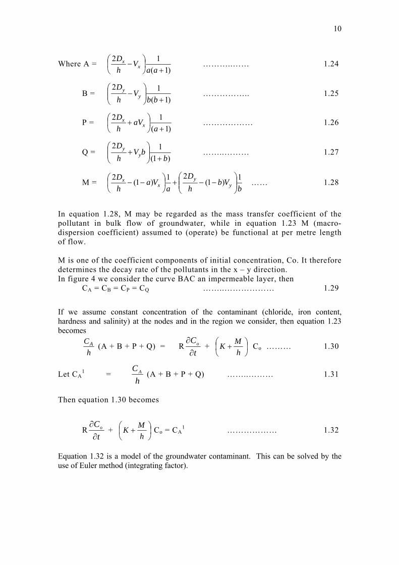
In equation 1.28, M may be regarded as the mass transfer coefficient of the pollutant in bulk flow of groundwater, while in equation 1.23 M (macro-dispersion coefficient) assumed to (operate) be functional at per metre length of flow. M is one of the coefficient components of initial concentration, Co. It therefore determines the decay rate of the pollutants in the x – y direction. In figure 4 we consider the curve BAC an impermeable layer, then

CA = CB = CP = CQ ……..……………… 1.29

If we assume constant concentration of the contaminant (chloride, iron content, hardness and salinity) at the nodes and in the region we consider, then equation 1.23 becomes

h

CA (A + B + P + Q) = Rt

Co

+

h

MK Co ……… 1.30

Let CA1 =

h

C A (A + B + P + Q) ……..……… 1.31

Then equation 1.30 becomes

Rt

Co

+

h

MK Co = CA

1 ……………… 1.32

Equation 1.32 is a model of the groundwater contaminant. This can be solved by the use of Euler method (integrating factor).

11

2.3 Solution of the Model Equation Considering the fact that at stabilization, partial derivative changes to total derivative, equation 1.32 becomes:

R dt

dCo +

h

MK Co = CA

1 …..……… 1.33

or

dt

dCo + R

hMK )/( Co =

R

CA

1

…..……… 1.34

From equation 1.34, integrating factor, IF becomes

IF = exp.

R

h

MK )( .t …..……… 1.35

Multiplying equation 1.34 all through by IF we obtain

exp

R

h

MK )( .t

dt

dCo + exp.

R

h

MK )( .t

R

hMK )/( Co

R

CA1 exp.

R

h

MK )( .t …..……… 1.36

Integrating equation 1.36

tR

h

MKCd o .)(.exp =

t

oA tR

h

MK

R

C.)( exp.

1

dt ….. 1.37

Co. exp.

R

h

MK )( .t =

t

o

A

hMK

tRhMk

R

C

/

./)/(.exp1

Co. exp.

R

h

MK )( .t =

)/(

1

hMK

CA

(exp.

R

h

MK )( .t – 1) …... 1.38

Co = )/(

1

hMK

CA

tR

h

MK .exp

11

12

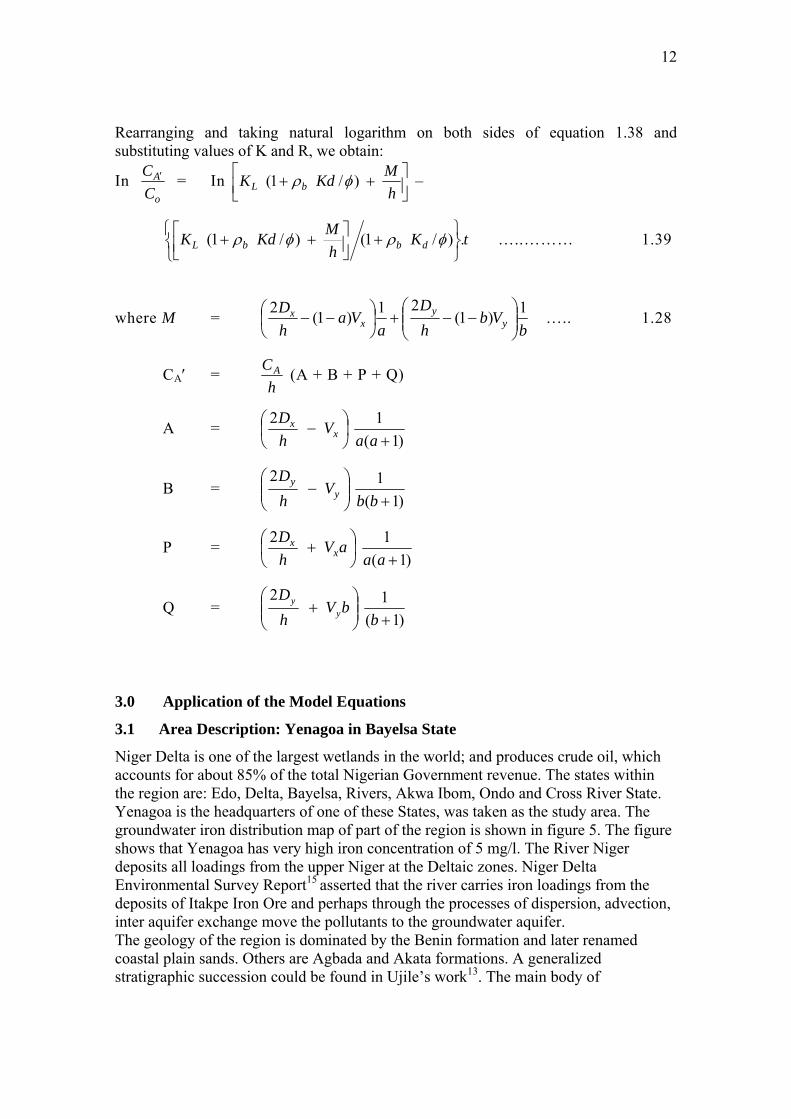
Rearranging and taking natural logarithm on both sides of equation 1.38 and substituting values of K and R, we obtain:

In o

A

C

C = In

h

MKdK bL )/ 1( –

tKh

MKdK dbbL .)/ 1( )/ 1(

…..……… 1.39

where M = b

Vbh

D

aVa

h

Dy

yx

x 1)1(

21)1(

2

….. 1.28

CA = h

CA (A + B + P + Q)

A = )1(

1

2

aa V

h

Dx

x

B = )1(

1

2

bb V

h

Dy

y

P = )1(

1

2

aaa V

h

Dx

x

Q = )1(

1

2

bb V

h

Dy

y

3.0 Application of the Model Equations

3.1 Area Description: Yenagoa in Bayelsa State

Niger Delta is one of the largest wetlands in the world; and produces crude oil, which accounts for about 85% of the total Nigerian Government revenue. The states within the region are: Edo, Delta, Bayelsa, Rivers, Akwa Ibom, Ondo and Cross River State. Yenagoa is the headquarters of one of these States, was taken as the study area. The groundwater iron distribution map of part of the region is shown in figure 5. The figure shows that Yenagoa has very high iron concentration of 5 mg/l. The River Niger deposits all loadings from the upper Niger at the Deltaic zones. Niger Delta Environmental Survey Report15 asserted that the river carries iron loadings from the deposits of Itakpe Iron Ore and perhaps through the processes of dispersion, advection, inter aquifer exchange move the pollutants to the groundwater aquifer. The geology of the region is dominated by the Benin formation and later renamed coastal plain sands. Others are Agbada and Akata formations. A generalized stratigraphic succession could be found in Ujile’s work13. The main body of

13

groundwater in major parts is contained in very thick and extensive sand and gravel aquifers of the Benin formation

Fig. 5 Groundwater Iron distribution map of Bayelsa and Rivers State in Niger Delta

The River Niger bifurcates at some 130 km south of the apex into the rivers Nun and

Forcados. Yenagoa is located east of the confluence of River Nun and Ekole river.

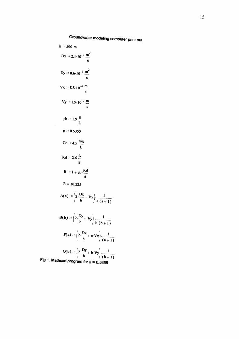
3.2 Application of the model The application of the model was carried out with the MATHCAD software systems. The expression in the parenthesis – (1 + ρb Kd / ) is called the retardation factor. This expression determines the resistance of the contaminant to move through the groundwater aquifer. The analysis of the parameter effective porosity was based on the transient characterization and its effect on the groundwater flow systems. MATHCAD program was developed from the solution of the model equation, and the results are shown on the computer print out as shown in Appendices 1 to 5. The input data for Yenagoa based on the hydrogeological features are: Boundary Conditions 0 ≤ x ≤ 500 0 ≤ y ≤ 49.5 For h = 500m; a = (0.1 – 1.0); b = (0.009 – 0.099); Co = 4.5 mg/l (iron content). Other input data are shown in Appendix 1 and the output indicated from Appendices 2 to 5.

14

4.0 Results and Discussion

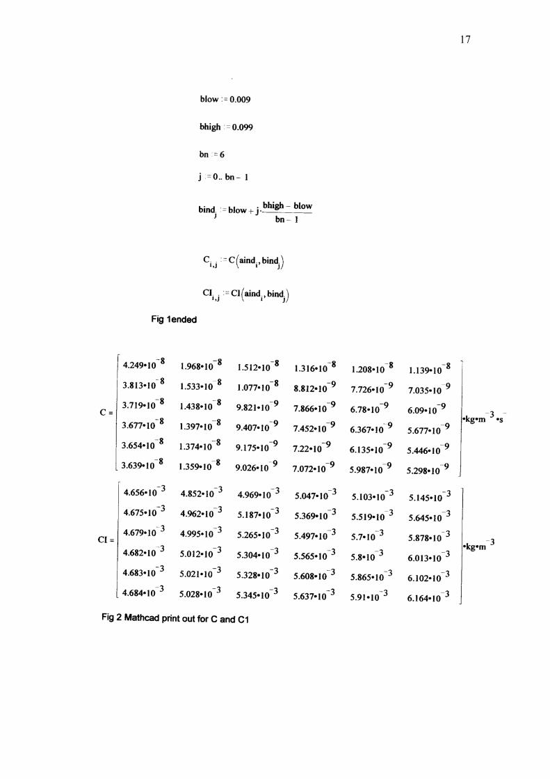
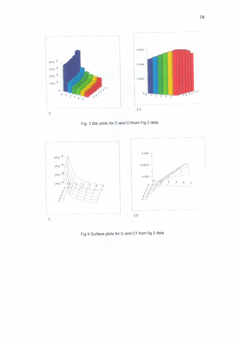
The results obtained in the form of matrix of function values, surface, bar and contour plots over specified horizontal and vertical ranges show rapid divergent when effective porosity is increased. For conservation transport model, the following observations are made: A reduction in contaminant concentrations with increase in porosity values provides primary lines of evidence for natural attenuation of each contaminant. The contour plots provide secondary evidence for possible biodegradation of contaminant in a spatial trend analysis. These observations may be correct for conditions where there are spillages of chemicals, dumpsites of municipal and hazardous wastes. However, the high iron content and hardness levels detected in most groundwater in the region especially in Yenagoa has been traced to the upcoming deposits from the Niger Delta river system distributions which affect the groundwater by processes of diffusion, advection, convection via interaquifer exchange, direct migration, infiltration and groundwater/ surface water interaction. Therefore the source of the contamination seems to be natural. Then attenuation and biodegradation phenomenon may not apply in the circumstance. For non conservative transport model, the following observations are made: An increase in contaminant concentrations with increase in porosity values shows that natural attenuation may not be tenable. The alternative solution to the groundwater problem will be to analyze borehole samples and the results determine the treatment method(s) to be applied to obtain potable water. For the non-conservative transport model there is increase in the contaminant concentration, as it moves from source to sink. The model equation has proved that the concentration levels of iron pollutant in groundwater depend on distance from source of pollution, time and processes transfer and the regime of flow. The distribution map of iron concentration was considered for comparison of the simulated model output. The MATHCAD graphical representations of C and C1 for Yenagoa compare the distribution of the contaminants. C on the printout shows the gradual penetration of the dissolved molecules of the contaminant into groundwater when there is no reaction. Comparison with C1 shows the change owing to the reaction with first order decay rate. As time elapses the concentration profiles with reaction, take on a different shape and approach a limiting exponential profile for which reaction and diffusion are in step at each value of boundary conditions. The profile remains steady because the rate of diffusion at each value of h, a, b (which determine the y and x positions) is exactly equal to the total rate of reaction throughout the aquifer length, x and depth, y. When these occur, there is no further decrease in the mass transfer rate of contaminants into the groundwater bodies. The print out result shows that at x direction concentration of contaminant increases on the surface and decreases in the y-direction perhaps owing to adsorption processes in the rock matrix. The surface, bar and contour plots of C and C1 illustrate the spatial distribution of contaminants without reaction and with first order reaction respectively.

15

16

17

18

19

20

5.0 Conclusions

The solution to second order partial differential equations for groundwater flow has been obtained. The application of the model equation has provided results that are similar to other work carried out by other researchers with complex results The variation of porosity values has caused significant changes in the concentration of groundwater contaminant. This analysis can be applied for the design of natural attenuation landfill for both municipal and industrial wastes. Materials of construction at the bottom of the landfill can be based on the principle of attenuation of groundwater contaminants. The reaction that is simulated is non-linear equilibrium adsorption of a single dissolved species. However several different zones with different sorptive and reactive properties are required: e. g distribution coefficient, decay coefficient, yield coefficient. It is therefore recommended that further analysis/ research on the model equations developed by the author be carried out as to determine the impact of soil bulk density, chemical decay rates and other hydro geological parameters on groundwater contamination. Federal and State Ministries of Environment should consider groundwater protection an issue of paramount importance. Enabling Laws should be put in place for waste disposal systems and these Laws should be enforced. 6.0 Nomenclature C = Conc. of the contaminant at time t, (for conservative transport model),mg/Ls C1 = Concentration of the contaminant at time t, with 1st order reaction (for non conservative transport model), mg/L Co = Initial concentration of the contaminant mg/Ls Dx, Dy, = Directional hydrodynamic dispersion coefficients, m2 / s exp = exponent ln = Natural logarithm h = Distance of flow moved by pollutant; m Kd = Distribution coefficient. Kl ,Ks = First order decay rate in the liquid phase and soil respectively, 1/s K = Overall first order decay rate = Kl + Ks ρb Kd / , 1/s.. l = Characteristic linear dimension, m. M = Bulk mass transfer coefficient of pollutant in groundwater flow in x-y direction, m/s flow in x-y direction, m/s. R = Retardation factor = 1 + ρb Kd / . t = Process time, or time since the start of the simulation, s. Vx, Vy = Directional seepage velocity components, m/s

Greek letter = Effective porosity; porosity of aquifer

ρb = bulk density of soil, kg/m3

21

REFERENCES

1 Chrysikopoulos, C. V; Hsuan, P.Y; Fyrillas, M. M. and Lee, K. Y.(2003): Mass Transfer Coefficient and Concentration boundary layer thickness for a dissolving (non-aqueous phase liquid) NAPL pool in porous media. In: Journal of Hazardous Material. B97, pp 245-255 2 Mercer, J. W; Lyle, R S and Charles, R F.(1983): Modeling Ground- Water Flow at Love Canal, New York In: Journal of Environmental Engineering. Vol. 109 No. 4.pp 924-941 3 Bredehoeft, J. D. and Pinder, G. F. (1973): Mass Transport in Flowing Groundwater: Water Resources Research 9 (1) 194-210 4 Schwartz, W. F; Cherry, A. J; and Roberts, R. J.(1982): A case study of a chemical spill; Polychlorinated Biphenyls (PCBs) in hydrogeological conditions and contaminant migrations. Water Resources Research ,Vol..18 No. 3 pp 535-545 5 Ashim, D.G; Poojitha, N. D and Yapa, D (1982): Salt Water Encroachment in an Aquifer. Water Resources Research.Vol. 18 No. 3 pp 546-550 6 Abraham, M. (1976): Nitrate and Chloride Pollution of Aquifers: A Regional Study with the Aid of a single-cell model, Water Resources Research- August, 1976, Vol.12; No. 4 pp731-732 .7 Spanoudaki, K; Nanou, A; Stamou, A. I; Christodoulou, G; Sparks, T; Bockelmann, B. and Falconer, R.A.(2005): Integrated Surface Water-Groundwater Modeling. In: Global Nest Journal vol.7 No.3 pp 281-295 8 Shahld, S and Rahman, M. M. (2004): Modeling Groundwater Flow for the delineation of wellhead Protection area around a water well. In: Journal of spatial Hydrology. Vol. 4. No. 1 9 Fatta, D; Naoun, C; Karlis, P; and Loizidou, M (2000). Numerical Simulation of Flow and Contaminant Migration at a Municipal Landfill. In: Journal of the International Association for Env. Hydrology. Vol. 8 10 Park, J; Bethke, C. M; Torgerson, T. and Johnson, T. M (2002): Transport Modeling applied to the interpretation of Groundwater 36Cl age. In: Water Resources Research. Vol.38. No.5 11 Stefan, H and Hermann, k. (2003): Geometric Analysis and Non Linear Partial Differential Equations. http://www.Spriger.de © Springer.Verlag.BerlinHeldelberg. 12 NRC (1994): National Research Council, Alternatives for Groundwater Clean Up. National Academy Press pp 336. 13 Ujile, A A (2003): Modeling Groundwater Contaminants due to Transient Sources of Pollutants. PhD Dissertation. RSUST, Nigeria 14 Anderson, M. P (1979): Using Models to simulate the Movement of Contaminants through Groundwater Flow systems, CRC Critical Review in Environmental Control, No. 9, pp. 97-156 15 NDES Report (1998): Niger Delta Environmental Survey, Phase 2 Report. Hydrology and Hydrodynamics vol. 1. Hydrological Characteristics and Resources .