The Astronomical Journal, 135:72–82, 2008 January doi:10.1088/0004-6256/135/1/72c© 2008. The American Astronomical Society. All rights reserved. Printed in the U.S.A.

AN ORBITAL ELEMENT FORMULATION WITHOUT SOLVING KEPLER’S EQUATION

Toshio FukushimaNational Astronomical Observatory, Ohsawa, Mitaka, Tokyo 181-8588, Japan; Toshio.Fukushima@nao.ac.jp

Received 2007 August 1; accepted 2007 September 14; published 2007 November 29

ABSTRACT

Starting from a standard orbital element formulation adopting the mean anomaly or longitude as the elementrelated to time, changing its independent variable from the physical time to the corresponding eccentric angle, andreplacing the mean angle with the time element of Stiefel & Scheifele, we present a new orbital element formulationof perturbed two-body problems which requires no solution of Kepler’s equation.

Key words: celestial mechanics – methods: analytical – methods: numerical

1. INTRODUCTION

In order to study perturbed two-body problems, whethernumerically or analytically, the solution of Kepler’s equationis absolutely essential in almost all orbital element formulationsstarting from those of Lagrange and Gauss and includingquite a few variations of them (Brouwer & Clemence 1961;Pollard 1966; Battin 1987; Danby 1988; Bond & Allman1996; Roy 2002). No closed-form solution of the equationis known. Namely, its analytic solutions are expressed ininfinite series expansion. These are not effective in the case ofhighly eccentric orbits and/or for the purpose of high precisioncomputation. Therefore, the equation is numerically solved inpractical applications. Colwell (1993) details a long history ofseeking efficient numerical schemes to solve Kepler’s equationin a variety of forms. Recently a fairly fast procedure tosolve its standard elliptic form has been published (Feinstein& McLaughlin 2007). It is a refinement of our previouswork (Fukushima 1996b) based on the technique of dynamicprogramming. As for fast procedures of other forms such asthe extended elliptic, the standard hyperbolic, the extendedhyperbolic, the parabolic, the nearly parabolic, and the standarduniversal forms, see Fukushima (1999) and a series of our worksin its references. Despite the existence of such fast numericalprocedures, the complexity of solution of Kepler’s equation hasbeen an obstacle to developing suitable analytic theories or tointegrating practical problems numerically. Is this the fate oforbital element formulations in general?

One exception is the element formulation of Stiefel &Scheifele (1971). They introduced an additional transformationon the physical time to the Kustaanheimo–Stiefel (KS) regu-larization method (Kustaanheimo & Stiefel 1965). The trans-formed variable is called the time element. The independentvariable of their formulation is a sort of eccentric orbital longi-tude, i.e., the eccentric anomaly measured not from the pericen-ter but from a certain longitude origin on the osculating orbit.Meanwhile, their dependent variables are (1) the initial valuesof the KS position and velocity vectors, (2) the square root ofhalf the negative Kepler energy, and (3) the time element men-tioned above. This formulation has a couple of good properties.One is that all the dependent variables are constants or a linearfunction of the independent variable in unperturbed orbits. Thisis suitable in developing perturbation theories. Also their nu-merical integration suffers no truncation error for unperturbedorbits. The other benefit is that the physical position and velocityvectors as well as the physical time are explicitly described interms of the independent and dependent variables. As a result,

the right-hand sides of the evolution equation of the elementscontain no implicit expressions. Namely, there is no need tosolve any variant of Kepler’s equation. However, this schemehas two drawbacks. One is that the number of orbital elementsis as large as 10, the same as that of dependent variables in theoriginal KS regularization. This fact means that the transforma-tion between them and the physical variables is not one-to-one.This causes difficulties in evaluating partial derivatives correctlyand introduces much complexity in orbital improvements. Theother demerit is that they are well defined only in elliptic cases.This is due to the limited nature of the time element.

In order to alleviate the latter defect, Bond (1974) presentedits universal extension by inventing a universal time element. Headopted Sundman’s fictitious time as the independent variableand avoided the above singularity by tactfully utilizing variousformulas of special functions named Stumpff functions. Thenumber of orbital elements remains 10. The extended schemecontains the independent variable explicitly in the evolutionequation of elements. This causes mixed secular terms in de-veloping analytic solutions, and is thus troublesome. There-fore, he also provided a further modification in order to avoidsuch direct appearance at the cost of adding two more ele-ments to be integrated. As a result, the number of elementsincreases to 12. Later, Bond and his coworkers created anotheruniversal formulation of orbital elements based on the Sperling–Burdet regularization method (Sperling 1961; Burdet 1967;Burdet 1968). Their works are summarized in Bond & Allman(1996). In this case, the number of orbital elements is as largeas 15.

In summary, the numbers of orbital elements in the existingformulations without solving Kepler’s equation are as large as10, 12, or 15. This indicates that the orbital elements adoptedare not independent of each other. In other words, we not onlyface extra computational time and additional source of errors innumerical integration of the evolution equation but also muchcomplexity and surplus labor in developing perturbation theoriesanalytically. In order to overcome this situation, we present anew formulation of the orbital elements avoiding the usage ofKepler’s equation and yet with the minimal number of dependentvariables, 6. Starting from standard element formulations usingthe osculating mean angles as the element related to time, we(1) replace the mean angles with the corresponding eccentricones, (2) introduce a new time-like argument linear with respectto the adopted eccentric angles, and (3) exchange the role ofthe independent and dependent variables between the adoptedeccentric angles and the introduced time-like argument. As aresult, the new formulation uses six orbital elements as its set

72

No. 1, 2008 AN ORBITAL ELEMENT FORMULATION 73

of dependent variables and does not require Kepler’s equationto be solved.

2. METHOD

2.1. Standard Orbital Element Formulation

Consider perturbed two-body problems. The equations ofmotion in Cartesian coordinates are given as

d rdt

= v,dv

dt= −µr

r3+ a, (1)

with the initial conditions,

r = r0, v = v0, when t = t0. (2)

Here t is the physical time, r and v are the physical po-sition and velocity vectors, r ≡ |r| is the radius vector,a is the physical perturbative acceleration, which is, in general,a function of t , r , and v as

a = a(t, r, v), (3)

µ is the gravitational constant of the two-body problem, t0 isthe initial epoch, and r0 and v0 are the initial values of r and v,respectively.

To simplify descriptions in the following, we classify orbitalelements into two categories: (1) that directly connected tot , and (2) the other five elements. We denote by C thelatter elements collectively. There are a variety of choicesfor the former element. Among them, we consider using M ,the osculating mean anomaly. This is in order to avoid theoccurrence of so-called mixed secular terms (refer to Chapter 4,Section 5 of Pollard 1966). Throughout this paper, we usethe word “element” in a broad sense, namely as a quantityreducing to a constant or a linear function of the independentvariable under no perturbations (Stiefel & Scheifele 1971). Interms of the independent and dependent variables describing theorbital motions, to adopt this element formulation is to conducta variable transformation from (t; r, v) to (t;C,M).

In any event, the transformation from the elements to positionand velocity is not given in a closed form. Instead, r and vare expressed as explicit functions of C and the trigonometricfunctions of an intermediate angle variable called the osculatingeccentric anomaly, E, as

r = r(C, sin E, cos E), v = v(C, sin E, cos E). (4)

Note that neither t nor M appears directly here. Also, E itselfdoes not appear either. The angle E is determined from M bysolving the standard elliptic form of Kepler’s equation,

E − e sin E = M, (5)

where e is the orbital eccentricity. Sometimes another anglevariable, called the true anomaly, f , is used in place of E. Theexpressions in terms of sin f and cos f are calculated by usingsin E and cos E as

sin f = (√

1 − e2) sin E

1 − e cos E, cos f = cos E − e

1 − e cos E. (6)

In any event, the flow of computing process goes like this:(1) once C and M are given, E is obtained as a solution of

Kepler’s equation, (2) sin E and cos E are evaluated from E,(3) if necessary, sin f and cos f are calculated from sin E andcos E by using the above transformation formula, and (4) r andv are calculated from C, sin E, and cos E, and/or sin f and cos fby standard procedures such as given in Brouwer & Clemence(1961).

On the other hand, the equations of time evolution of theelements are expressed as a system of first-order ordinarydifferential equations as

dC

dt= FC,

dM

dt= n + FM, (7)

where FC and FM are perturbative quantities in the sense theyreduce to zero under no perturbations. Also

n ≡√

µ

a3(8)

is the osculating mean motion and

a ≡ µr

2µ − rv2(9)

is the osculating semimajor axis, the latter usually being chosenas one of orbital elements. Obviously both n and a are functionsof r and v only.

There are two styles to express FC and FM : one to providethem as linear combinations of Cartesian components of a asGauss provided, and the other based on partial derivatives of acertain function V as Lagrange obtained when the perturbingaccelerations are derived from a perturbing potential. In anycase, the evolution equation is given as a result of transformationof the equation of motion into those of time derivatives ofthe elements (Pollard 1966). Specific functional forms of FC

and FM in terms of C, sin E, cos E, sin f , cos f , and a or∂V/∂C plus other partial derivatives can be seen in standardtextbooks on celestial mechanics (Danby 1988; Roy 2002).The original expression of evolution equations developed byLagrange, Gauss, and their followers contain all of sin E, cos E,sin f , and cos f in a mixed manner (Brouwer & Clemence1961). The expression using sin f and cos f only is foundin Chapter 1, Section 17 of Pollard (1966). The expressionusing sin E and cos E only could be derived from this using thetransformation formulas of sin f and cos f given above.

As for the dependence on the main angle variable, E or f ,its sine and cosine functions only appear in these procedures.Namely, the angle variable itself is not explicitly used in thisformulation. As a result, there is no direct appearance of E, f ,or t itself in the orbital element formulations adopting M asthe element related to the physical time. This feature enables usto avoid the so-called mixed secular terms, which are harmfulnot only in constructing analytic theories but also conductingnumerical integrations in the long run.

2.2. Elimination of Kepler’s Equation

Let us remove the necessity to solve Kepler’s equation fromthe above formulation. For this purpose, we find a way tocompute E without using M . More specifically, we directlydefine E as an explicit function of r and v as

E ≡ tan−1

(B

√J

A

), (10)

74 FUKUSHIMA Vol. 135

where

J ≡ 2µ

r− v2, A ≡ rv2 − µ, and B ≡ r · v, (11)

are auxiliary functions of r and v. This definition is derived fromthe expressions of J , A, and B in terms of osculating quantitiesas

J = n2a2, A = µe cos E, and B = na2e sin E, (12)

and an osculating relation, µ = n2a3.Since this expression contains an ambiguity with multiples of

2π , we determine E by integrating a differential equation. Bydifferentiating the above defining relation of E and noting thatr and v are subject to the equations of motion, Equation (1), weimmediately obtain the time derivative of E as

dE

dt= na

r(1 + α), (13)

where

α ≡ r

µe

[(cos E)(r · a) −

(2 − e cos E) sin E

n

(v · a)

](14)

is a perturbative quantity. In deriving the above expression ofα, we used osculating relations of the radius vector and of theeccentricity as

r = a(1 − e cos E) and (µe)2 = A2 + JB2, (15)

and the expression of time derivative of J as

dJ

dt= −2(v · a), (16)

which is also obtained from Equation (1) directly.The above expression of dE/dt can also be derived by

combining the expressions of partial derivative of E with respectto v, which will be given later, and substituting it into a generalexpression of dE/dt , namely Equations (10.87) and (10.89) ofBattin (1987). In general, dE/dt does not reduce to a constanteven under no perturbations, i.e. when α = 0. Therefore, E isnot an element as long as t is the independent variable.

In order to resolve this issue, we introduce a time-likevariable, τ , to be used in place of t . More concretely, we defineτ as an explicit function of t , r , and v as

τ ≡ t +B

J, (17)

which is rewritten in terms of osculating quantities as

τ = t +e sin E

n. (18)

This expression reveals that τ thus defined is equivalent to thetime element of Stiefel & Scheifele (1971).

To show the characteristic of τ more clearly, let us express Mby using n and T , the time of pericenter passage, as

M = n(t − T ). (19)

By using the standard elliptic form of Kepler’s equation,Equation (5), and the above rewriting of the defining relation ofτ , Equation (18), we have a similar expression for E:

E = n(τ − T ). (20)

Under no perturbations, n and T are constants. Therefore, forunperturbed orbits, E is a linear function of τ in the same mannerthat M is a linear function of t . In this sense, we may call τ theeccentric time.

Since τ is explicitly defined as a function of t , r , and v above,we easily evaluate its time derivative as

dτ

dt= a

r(1 + β), (21)

where β is another perturbative quantity expressed as

β ≡ r

µ

[(r · a) +

(2e sin E

n

)(v · a)

]. (22)

Using the time differential formulas of E and τ , Equations (13)and (21), we change the independent variable from t to E whileregarding τ as the last dependent variable other than C. In termsof the combination of independent and dependent variables, weshift from (t;C,M) to (E;C, τ ).

The resulting equations of evolution with respect to E are

dC

dE= GC

1 + α,

dτ

dE= 1

n

(1 + β

1 + α

), (23)

where

GC ≡ rFC

na. (24)

Here α, β, and GC are all perturbative quantities. Since nbecomes a constant under no perturbations, τ is an elementin a broad sense if E is the independent variable. All of theperturbative quantities as well as n are explicit functions ofC, sin E, cos E, and a. Namely, there is no direct appearanceof the independent variable, E, on the right-hand sides of theabove evolution equations. As a result, there occur no difficultiesregarding mixed secular terms with respect to E.

In the above selection of a new set of variables, of course, onemay choose another combination, (τ ;C,E). However, we preferE to τ as the independent variable. This is because E frequentlyappears on the right-hand sides of the above evolution equationsin an explicit manner while τ enters there only indirectly, i.e.by way of t in the argument of a. From the viewpoint ofsolving ordinary differential equations, whether analytically ornumerically, it is wise to choose as the independent variableone whose explicit appearance is most significant on the right-hand sides. To examine this assertion more clearly, we comparethe difficulties in solving the following ordinary differentialequation in two ways:

dy

dx= f (y), and

dx

dy= 1

f (y). (25)

Obviously, the latter form is easier to solve since the problemreduces to integration of a known function of the independentvariable adopted.

2.3. An Example of New Formulation

Let us be more specific. As an illustration of C, we select aclassic set of five elements, (a, e, I, Ω, ω), which we collectivelyname X. Here I is the osculating inclination, Ω is the osculatinglongitude of ascending node, and ω is the osculating argumentof pericenter. Of course, this is not the only choice to which theformulation described in the previous subsection is applicable.

No. 1, 2008 AN ORBITAL ELEMENT FORMULATION 75

For example, we may replace a by L, the magnitude of specificangular momentum vector, as Pollard (1966) did. For cometaryorbits being nearly parabolic but still elliptic, it is customaryto replace a by (1) q ≡ a(1 − e), the osculating pericenterdistance, or (2) p ≡ a(1 − e2), the osculating semilatus rectum.In the case of small inclination orbits, we may use in place of thecombination of I and Ω: (1) the pair of sin I sin Ω and sin I cos Ωas we will use later, (2) the combination of sin(I/2) sin Ωand sin(I/2) cos Ω as given in Roy (2002), (3) the couple oftan I sin Ω and tan I cos Ω as provided in Brouwer & Clemence(1961), or (4) the choice of tan(I/2) sin Ω and tan(I/2) cos Ωas appearing in Broucke & Cefola (1972) and Battin (1987).Furthermore, one may adopt some vectorial elements such ascomponents of the orbital angular momentum vector, L ≡ r×v,or of the eccentricity vector, e ≡ (v × L)/µ − r/r as obtainedby Pollard (1966).

In any event, let us return to our choice, X. Once X and Eare given, the standard variables, t , r , and v, are calculated as

t = τ − e sin E

n, r = rP nP + rQnQ, v = vP nP + vQnQ,

(26)where the position and velocity components in the osculatingorbital plane are given as

rP = a(cos E − e), rQ = aeL sin E,

vP = −na sin E

r, vQ = naeL cos E

r.

(27)

HereeL ≡

√1 − e2, (28)

is the complementary eccentricity, and n and r are computedfrom a, e, and E as

n =√

µ

a3, r = a(1 − e cos E). (29)

Meanwhile, nP and nQ are vector functions of I , Ω, and ωonly. More concretely, these two unit vectors, together with nW ,which will be defined later, consist of a coordinate triad, i.e. a setof three orthonormal base vectors. The triad defines an orbitalreference frame whose x-axis is toward the pericenter, andwhose x–y plane is the osculating orbital plane. Mathematicallythey are expressed in terms of the fundamental rotation matrix,Rj (θ ), with −ω, −I , and −Ω as their Eulerian angles in the3–1–3 manner of rotation as

(nP , nQ, nW ) ≡ R3(−Ω)R1(−I )R3(−ω)

=(

cos Ω cos ω − sin Ω cos I sin ωsin Ω cos ω + sin Ω cos I sin ω

sin I sin ω

−cos Ω sin ω − sin Ω cos I cos ω sin Ω sin I−sin Ω sin ω + cos Ω cos I cos ω −cos Ω sin I

cos I sin ω cos I

).

(30)

Conversely, the new variables, (E; a, e, I, Ω, ω, τ ), are deter-mined from the old ones, (t; r, v), as

E = atan2(B√

J ,A), a = µ

J,

e =√

A2 + JB2

µ, I = atan2(LP ,LZ), (31)

Ω = atan2(LX,−LY ), ω = atan2(eM, eN ), τ = t +B

J,

where

r =√

r2, J = 2µ

r− v2, A = rv2 − µ,

B = r · v,

(LX

LY

LZ

)≡ L = r × v, LP =

√L2

X + L2Y ,

nN = 1

LP

(−LY

LX

0

), L =

√L2

P + L2Z, nW = L

L,

nM = nW × nN, e = v × Lµ

− rr, eN = e · nN,

eM = e · nM, (32)

and atan2(y, x) is the two-argument arc tangent function tocompute tan−1(y/x) while taking into account the signs of thearguments, x and y, and is realized in C and Fortran.

On the other hand, GX are expressed in terms of the newvariables and the perturbative acceleration as

Ga = 2a3

µ(Re sin E + SeL), (33)

Ge = a2eL

µ[ReL sin E + S2 cos E − e(1 + cos2 E)], (34)

GI = a2W

µ(ξ cos ω − η sin ω), (35)

GΩ = a2W

µ sin I(ξ sin ω + η cos ω), (36)

Gω = a2

µe[−ReL(cos E − e) + S sin E(2 − e cos E − e2)]

− GΩ cos I, (37)

where

ξ ≡ cos ω

eL

[cos E − 2e(2 cos2 E − 1) + e2 cos E],(38)

η ≡ sin E(1 − e cos E),

and

R ≡ a · nR, S ≡ a · nS, W ≡ a · nW, (39)

are the well-known notations of perturbative acceleration com-ponents according to Gauss (Brouwer & Clemence 1961). Atrio of nR , nS , and nW is another coordinate triad defining theosculating orbital plane (Pollard 1966) whose x-axis is towardthe direction of r as

nR ≡ rr, (40)

where nW is already defined above, and as a result, the last basevector is defined as

nS ≡ nW × nR. (41)

The expressions of dE/dt and dτ/dt are also derived fromthose of M , e, and a as

dE

dt= 1

1 − e cos E

[dM

dt+

(de

dt

)sin E

], (42)

76 FUKUSHIMA Vol. 135

dτ

dt= 1 +

e cos E

n

(dE

dt

)+

sin E

n

(de

dt

)+

3e sin E

2na

(da

dt

).

(43)These lead to the expressions of α and β in terms of R and S as

α = a2

µe[R(cos E − 2e + e2 cos E) − SeL sin E(2 − e cos E)],

(44)β = a2

µ[R1 − 2e cos E + e2(2 − cos2 E) + 2SeLe sin E].

(45)

These rewritings are also obtained directly from Equations (14)and (22) by using the osculating relations

r · a = Rr, v · a =(

na2

r

)(Re sin E + SeL). (46)

The above expressions of α, β, and GX contain no singularity ofthe form of 1/r . This is because such singularities existing in theexpressions of v · a and Fa are removed by multiplying by r .

Finally, the initial conditions of the evolution equation aresimply given as

X = X0, τ = τ0, when E = E0, (47)

where the quantities with the subscript 0 are their initial values,which are explicitly obtained from those of t , r , and v by usingthe reverse transformation procedure described above.

Reviewing the above, we learn that (1) the number of newdependent variables, (a, e, I, Ω, ω, τ ), is six, the minimum, (2)r and v are directly expressed as analytic functions of a, e,I , Ω, ω, sin E, and cos E, (3) t is explicitly evaluated froma, e, τ , and sin E, (4) the reverse transformation from the oldvariables, (t; r , v), to the new ones, (E; a, e, I, Ω, ω, τ ), is alsoexplicit, (5) all the right-hand sides of the evolution equationswith respect to E either vanish or reduce to a constant whenunder no perturbations, and thus (6) all the new variables areelements, (7) all the right-hand sides of the evolution equationsare explicit functions of a, e, I , Ω, ω, sin E, and cos E, and as aresult, (8) there appear no mixed secular terms in their analyticsolutions. Therefore, we arrive at a formulation (1) using sixelliptic orbital elements, (2) avoiding the singularity of 1/r ,(3) causing no mixed secular terms in analytic developments,and (4) not requiring any form of Kepler’s equation to be solved.

2.4. Exclusion of Small Divisors

In the formulation obtained in the previous subsection,there still remain some mathematical singularities. They resultfrom small divisors as e or sin I in the expressions of theevolution equations. These singularities are spurious since theyare caused by an inappropriate choice of orbital elements. Inorder to remove these fake singularities, one usually adds toM and/or E other angles such as the longitude of pericenter, ≡ Ω + ω (Pollard 1966). Therefore, we replace the previousset of independent and dependent variables, (E;X, τ ), by a newcombination, (D;Y, τ ). Here D ≡ E + is the osculatingeccentric orbital longitude and Y is a set of nonsingularorbital elements, (a, eJ , eK, gX, gY ), which consists of part ofa variation of equinoctial elements (Broucke & Cefola 1972).More specifically, we introduce new orbital elements as

eJ ≡ e cos , eK ≡ e sin ,

gX ≡ sin I sin Ω, gY ≡ −sin I cos Ω,(48)

which are well defined even in the limit e → 0 and/or I → 0.

Although many textbooks refer to the existence of suchnonsingular elements, their full treatment is rarely found inthe literature. Thus, we present their details here. First, thetransformation from (D;Y, τ ) to (t; r, v) becomes

t = τ − eS

n, r = rJ nJ + rK nK, v = vJ nJ + vK nK.

(49)

Here

eS ≡ e sin E = eJ sin D − eK cos D, n ≡√

µ/a3. (50)

Also, we introduce Broucke’s equinoctial coordinate triad,(nJ , nK, nW ), defining the osculating orbital plane. The triadis explicitly defined as functions of gX and gY as

nJ ≡(

1 − gXX

−gXY

−gX

), nK ≡

( −gXY

1 − gYY

−gY

), nW ≡

(gX

gY

gZ

),

(51)where

gXX ≡ g2X

1 + gZ

, gXY ≡ gXgY

1 + gZ

,

gYY ≡ g2Y

1 + gZ

, gZ ≡√

1 − (g2

X + g2Y

).

(52)

The functional form contains no trigonometric functions, whichare much more time-consuming than the square root and divisionoperations. This is the reason why we prefer the pair of gX andgY in place of a more popular combination, I sin Ω and I cos Ω.

The relations among the used sets of coordinate triads aregiven in terms of rotation matrices as

(nR, nS, nW ) = R3(f )(nP , nQ, nW )

= R3(f + ω)(nN, nM, nW )

= R3(f + ω + Ω)(nJ , nK, nW ), (53)

which is decomposed in vector components as

nR = nP cos f +nQ sin f, nS = −nP sin f +nQ cos f, (54)

nP = nN cos ω + nM sin ω, nQ = −nN sin ω + nM cos ω,(55)

nN = nJ cos Ω + nK sin Ω, nM = −nJ sin Ω + nK cos Ω.(56)

On the other hand, the components of the position and velocityvectors in the osculating orbital plane, rJ , rK , vJ , and vK , aredefined as functions of a, eJ , eK , sin D, and cos D as(

rJ

rK

)≡ a

(−eJ + (1 − eKK ) cos D + eJK sin D−eK + eJK cos D + (1 − eJJ ) sin D

), (57)(

vJ

vK

)≡ na

1 − eC

(−(1 − eKK ) sin D + eJK cos D−eJK sin D + (1 − eJJ ) cos D

), (58)

whereeC ≡ e cos E = eJ cos D − eK sin D, (59)

and

eJJ ≡ e2J

1 + eL

, eJK ≡ eJ eK

1 + eL

,

eKK ≡ e2K

1 + eL

, eL ≡√

1 − (e2J + e2

K

).

(60)

No. 1, 2008 AN ORBITAL ELEMENT FORMULATION 77

Second, the reverse transformation from (t; r, v) to (D;Y, τ ) isgiven as

D = atan2(sD, cD), a = µ

J,

(eJ

eK

)=

(e · nJ

e · nK

),

(gX

gY

gZ

)= L

L, τ = t +

r · vJ

, (61)

where (cD

sD

)≡ 1

eL

((1 − eJJ )hJ − eJKhK

−eJKhJ + (1 − eKK )hK

),

(62)(hJ

hK

)≡

(eJ + J (r · nJ )/µ

eK + J (r · nK )/µ

).

Here e, L, and J were provided in the previous subsection. AlsonJ , nK , eJJ , eJK , and eKK are computed from gX, gY , gZ , eJ ,and eK as in the transformation procedure to r and v. In derivingthe above expressions of cD and sD , we used an identity relation,

(1 − eJJ )(1 − eKK ) − e2JK = eL. (63)

Third, we obtain the time derivative of D from its definition as

dD

dt= dE

dt+

dω

dt+

dΩdt

= na

r(1 + γ ), (64)

where

γ ≡ α + Gω + GΩ

= a2

µ

[R

−2 + eL +

(2 + eL

1 + eL

)eC

+ S

(eS

1 + eL

)(e2

1 + eL

− eC

)]−

(aW

µ

)rL, (65)

is a new perturbative quantity and

rL ≡(

1 − eC

eL

) (gXrJ + gY rK

1 + gZ

). (66)

Similarly, β is expressed in terms of D and other osculatingquantities as

β = a2

µ

[R

(1 − 2eC + e2 − e2

C

)+ 2SeLeS

]. (67)

Using these expressions, we obtain the associated evolutionequation as

dY

dD= GY

1 + γ,

dτ

dD= 1

n

(1 + β

1 + γ

), (68)

where GY is expressed in its components as

Ga =(

2a3

µ

)(ReS + SeL), (69)

GeJ=

(a

µ

)[ReLrK + S[eLrJ + r(1 − eJJ ) cos D

− eJK sin D] − WeKrL], (70)

GeK=

(a

µ

)[−ReLrJ + S[eLrK + r−eJK cos D

+ (1 − eKK ) sin D] − WeJ rL], (71)

GgX=

(rW

µ

) [gXgY rJ +

(1 − g2

X

)rK

], (72)

GgY= −

(rW

µ

) [(1 − g2

Y

)rJ + gXgY rK

], (73)

wherer = a(1 − eC). (74)

These forms of β, γ , and GY contain no small divisors as e orsin I , as we expected.

3. NOTES

3.1. Application of Encke’s Method

Encke’s method is generally interpreted as an approach totransform dependent variables to their deviations from unper-turbed solutions, and to integrate the deviations in a manneravoiding loss of information caused by subtraction of quantitiesof the same order of magnitude. Originally it was developedby Encke to accelerate the numerical integration of cometaryorbits in Cartesian coordinates (Brouwer & Clemence 1961).Nevertheless, its application is meaningful even for orbital el-ement formulations. In particular, it is suitable for deriving thefirst-order analytic solutions. Furthermore, it effectively reducesround-off errors in numerical integration (Fukushima 1996a).

Let us apply this idea to the first combination of new variables.Namely, we move from the original variables (E;X, τ ) to theirdeviations (∆E; ∆X, ∆τ ), which are defined as

∆E ≡ E − E0, ∆X ≡ X − X0, ∆τ ≡ τ − τ0 − ∆E

n0,

(75)

where the quantities with the subscript 0 are the initial values.The evolution equations of the deviation variables are expressedin a form minimizing the information loss as

d(∆X)

d(∆E)= GX

1 + α,

(76)d(∆τ )

d(∆E)= 1

n0(1 + α)

[β − α −

(∆n

n

)(1 + β)

],

where

∆n

n≡ n − n0

n= −∆a

a0

(1 +

a

a0 +√

aa0

), (77)

and a ≡ a0 +∆a. The initial conditions of the deviation variablesare

∆X = 0, ∆τ = 0 when ∆E = 0. (78)

On the right-hand sides of the above evolution equations, oneshould understand that E, X, and τ are computed from ∆E, ∆X,and ∆τ as

E ≡ E0 + ∆E, X ≡ X0 + ∆X, τ ≡ τ0 +∆E

n0+ ∆τ.

(79)From a numerical point of view, the key is the expression of∆n not in the form of subtraction as n − n0 but in terms of ∆a,which are directly obtained through the integration procedure.

78 FUKUSHIMA Vol. 135

As a byproduct, the first-order perturbation theories aresimply obtained from the transformed evolution equations byignoring the second and higher order quantities as

d(∆X)

d(∆E)≈ GX,

d(∆τ )

d(∆E)≈ 1

n0

[β − α +

(3∆a

2a0

)],

(80)approximating all the elements on the right-hand sides by theirunperturbed solutions as

X ≈ X0, τ ≈ τ0 +∆E

n0, (81)

integrating the evolution equations of ∆X with respect to ∆E bytaking care of the initial conditions as

X(1) = X0 +∫ E−E0

0GXd(∆E), (82)

and integrating the evolution equation of ∆τ as

τ (1) = τ0 +1

n0

∫ E−E0

0(β − α)d(∆E)

+3

2n0a0

∫ E−E0

0

(∫ ∆E

0Gad(∆E)

)d(∆E), (83)

where ∆a in the integrand of the second integral in the lastprocedure is approximated by the first-order solution obtainedin the third procedure.

The same approach can be taken to the other set of variables;from (D;Y, τ ) to (∆D; ∆Y, ∆τ ). In this case, the evolutionequations become

d(∆Y )

d(∆D)= GY

1 + γ,

(84)d(∆τ )

d(∆D)= 1

n0(1 + γ )

[β − γ −

(∆n

n

)(1 + β)

].

3.2. Partial Derivatives

The number of new dependent variables is six, the same as thatof the standard ones. Also the standard variables are expressedas explicit functions of the new variables as

t = t(E, a, e, τ ), r = r(E, a, e, I, Ω, ω),

v = v(E, a, e, I, Ω, ω). (85)

Therefore, it is straightforward to obtain the partial derivativeof the old variables, (t; r, v), with respect to the new variables,(E; a, e, I, Ω, ω, τ ), as

∂t

∂E= −e cos E

n,

∂ r∂E

= rv

na,

∂v

∂E= −na2r

r2,

(86)

∂t

∂a= −3e sin E

2na,

∂ r∂a

= ra,

∂v

∂a= −v

2a, (87)

∂t

∂e= −sin E

n,

∂ r∂e

= −a

[nP +

(e sin E

eL

)nQ

],

∂v

∂e=

(na2 cos E

2eLr2

)(−rQnP + rP nQ), (88)

∂t

∂I= 0,

∂ r∂I

= (rP sin ω + rQ cos ω)nW,

∂v

∂I= (vP sin ω + vQ cos ω)nW,

∂t

∂Ω= 0,

∂ r∂Ω

= (rP cos ω − rQ sin ω)nL

− [(rP sin ω + rQ cos ω) cos I ]nN, (89)

∂v

∂Ω= (vP cos ω − vQ sin ω)nL

− [(vP sin ω + vQ cos ω) cos I ]nN, (90)

∂t

∂ω= 0,

∂ r∂ω

= −rQnP + rP nQ,

(91)∂v

∂ω= − vQnP + vP nQ,

∂t

∂τ= 1,

∂ r∂τ

= 0,∂v

∂τ= 0, (92)

where the unit vectors, nP , nQ, nW , and nN were provided inthe previous section and

nL ≡(−sin Ω

cos Ω0

). (93)

In order to interpret correctly the expressions of partial deriva-tives given here, one must understand the fixed variables. If wewrite the fixed variables explicitly, some of the above partialderivatives become as follows:

∂t

∂τ=

(∂t

∂τ

)E,a,e

,∂ r∂a

=(

∂ r∂a

)E,e,I,Ω,ω

,

(94)∂v

∂I=

(∂v

∂I

)E,a,e,Ω,ω

.

For example, the expression of ∂ r/∂e presented here differsfrom that of ∂ r/∂e in Chapter 4, Section 6 of Pollard (1966)since the former is the value when E, a, I , Ω, and ω are fixedwhile the latter is the value when M , a, I , Ω, and ω are fixed.This is because M varies according to the change in e when Eis fixed.

On the other hand, the inverse partial derivatives, i.e. thepartial derivatives of the new variables, (E; a, e, I, Ω, ω, τ ),with respect to the old ones, (t; r, v), are calculated as

∂E

∂t= 0,

∂E

∂ r= 1

ae

[a2(1 − e cos E − e2 cos2 E) sin E

r3

rT

+

(cos E

na

)vT

],

∂E

∂v= 1

nae

[(cos E

a

)rT −

(2 − e cos E) sin E

na

vT

],

(95)

No. 1, 2008 AN ORBITAL ELEMENT FORMULATION 79

∂a

∂t= 0,

∂a

∂ r=

(2a2

r3

)rT ,

∂a

∂v=

(2a2

µ

)vT ,

(96)∂e

∂t= 0,

∂e

∂ r= 1

µ

[(r · nP )rT − (v · nP )vT +

(v2 − µ

r

)nT

P

], (97)

∂e

∂v= 1

µ

[2(v · nP )rT − (r · nP )vT − (r · v)nT

P

],

∂I

∂t= 0,

∂I

∂ r= −(v × nM )T

L,

∂I

∂v= (r × nM )T

L,

(98)

∂Ω∂t

= 0,∂Ω∂ r

= (v × nN )T

L sin I,

∂Ω∂v

= −(r × nN )T

L sin I,

(99)

∂ω

∂t= 0,

∂ω

∂ r= 1

µe

[(r · nQ)rT − (v · nQ)vT +

(v2 − µ

r

)nT

Q

]

− cos I

(∂Ω∂ r

),

∂ω

∂v= 1

µe

[2(v · nQ)rT − (r · nQ)vT − (r · v)nT

Q

]− cos I

(∂Ω∂v

), (100)

∂τ

∂t= 1,

∂τ

∂ r= e cos E

n

(∂E

∂ r

)+

sin E

n

(∂e

∂ r

)+

3e sin E

2na

(∂a

∂ r

),

∂τ

∂v= e cos E

n

(∂E

∂v

)+

sin E

n

(∂e

∂v

)+

3e sin E

2na

(∂a

∂v

),

(101)

where T denotes the transpose of a column vector and

L ≡ |L| = na2eL (102)

is the magnitude of specific orbital angular momentum. Again,one must take account of fixed variables in understandingthe above expressions correctly. Some examples of rigorousexpressions are as follows:

∂E

∂t=

(∂E

∂t

)r ,v

,∂e

∂ r=

(∂e

∂ r

)t,v

,∂Ω∂v

=(

∂Ω∂v

)t,r

.

(103)

These expressions of partial derivatives are useful in orbitalimprovement and orbit design.

3.3. Expansion in Terms of Eccentric Anomaly

In developing analytic perturbation theories based on thenew formulation, we need the explicit expressions of variousquantities in terms of E as well as their Fourier expansions with

respect to E. Skipping the details, we present only the finalresults for some basic quantities other than M or r/a, which arealready provided, as

f = E + 2∞∑

k=1

(ekH

k

)sin kE, (104)

a

r= 1

eL

(∂f

∂E

)e

= 1

eL

(1 + 2

∞∑k=1

ekH cos kE

), (105)

cos f = −eH +

(2eL

1 + eL

) ∞∑k=1

ek−1H cos kE, (106)

sin f =(

2eL

1 + eL

) ∞∑k=1

ek−1H sin kE, (107)

where f is the true anomaly, and

eH ≡ e

1 + eL

= e

1 +√

1 − e2, (108)

is an auxiliary quantity. In the above, we quote Equation(19) of Chapter II of Brouwer & Clemence (1961) as Equa-tion (104), differentiate it with respect to E so as to obtainEquation (105), and rewrite cos f and sin f using Equation (6).

Since the coefficients in the above expansions are plainrational combinations of eH and eL, Fourier expansions ofmore general quantities such as (r/a)m exp(

√−1 kf ), wherem and k are arbitrary integers, are simply obtained by basicformula manipulations. Compare these expressions with similarexpansions in terms of M such as given in Brouwer & Clemence(1961). Obviously, the expressions in terms of E are simplerthan those in terms of M , which require the evaluation of Besselfunctions and their infinite summation.

3.4. Example of First-Order Analytic Treatment

Let us give an example of analytic treatments based on thenew formulations. Assume that the perturbation is of a drag-likenature such that the perturbative accelerations are given in theform

a = −cv, (109)

where c is, in general, a function of (1) v ≡ |v|, (2) thedensity of resistive media, and (3) some other quantities specificto the perturbed body such as the ratio of its cross sectionand mass (Pollard 1966; Battin 1987). The velocity vector isdecomposed into components with respect to the coordinatetriad, (nR, nS, nW ), as

v = BnR + LnS

r, (110)

where B and L are already defined as

B ≡ r · v = na2e sin E, L ≡ |L| = na2eL. (111)

Using the above decomposition, we derive the expression ofperturbative acceleration in the same reference frame as

R = −c

(na2e

r

)sin E, S = −c

(na2eL

r

),

(112)W = 0,

80 FUKUSHIMA Vol. 135

which lead to the more explicit expressions of α, β, and GX as

α = −c

(2

ne

)sin E,

β = −c( e

n

) [3 sin E +

( e

2

)sin 2E

],

Ga = −c

(2a2

n

)(1 + e cos E), Ge = −c

(2e2

L

n

)cos E,

GI = GΩ = 0,

Gω = +c

(2e3

L

ne

) (sin E

1 − e cos E

)

= +c

[4e3

L

ne(1 + eL)

] ∞∑k=1

ek−1H sin kE, (113)

where we used an identity relation

1 − e2H

eL

= 2

1 + eL

, (114)

in deriving the last expression.For simplicity, let us assume that c is a constant. Furthermore,

we ignore the contributions of α and β in the sums 1 + α and1 + β except the evolution equation of τ . Then, by integratingEncke’s form of evolution equations, we immediately obtain thefirst-order solutions of new orbital elements in terms of E as

a = a0 − c

(2a0

n0

)[(E − E0) + e0(sin E − sin E0)],

e = e0 − c

(2e2

L0

n0

)(sin E − sin E0),

I = I0, Ω = Ω0,

ω = ω0 − c

[4e3

L0

n0e0(1 + eL0)

] ∞∑k=1

ek−1H0

k(cos kE − cos kE0),

τ = τ0 +E − E0

n0+ c

(1

n20

)[(6e0 − 2

e0

)(cos E − cos E0)

+

(e2

0

4

)(cos 2E − cos 2E0) + (3e0 sin E0)(E − E0)

− 3

2(E − E0)2

], (115)

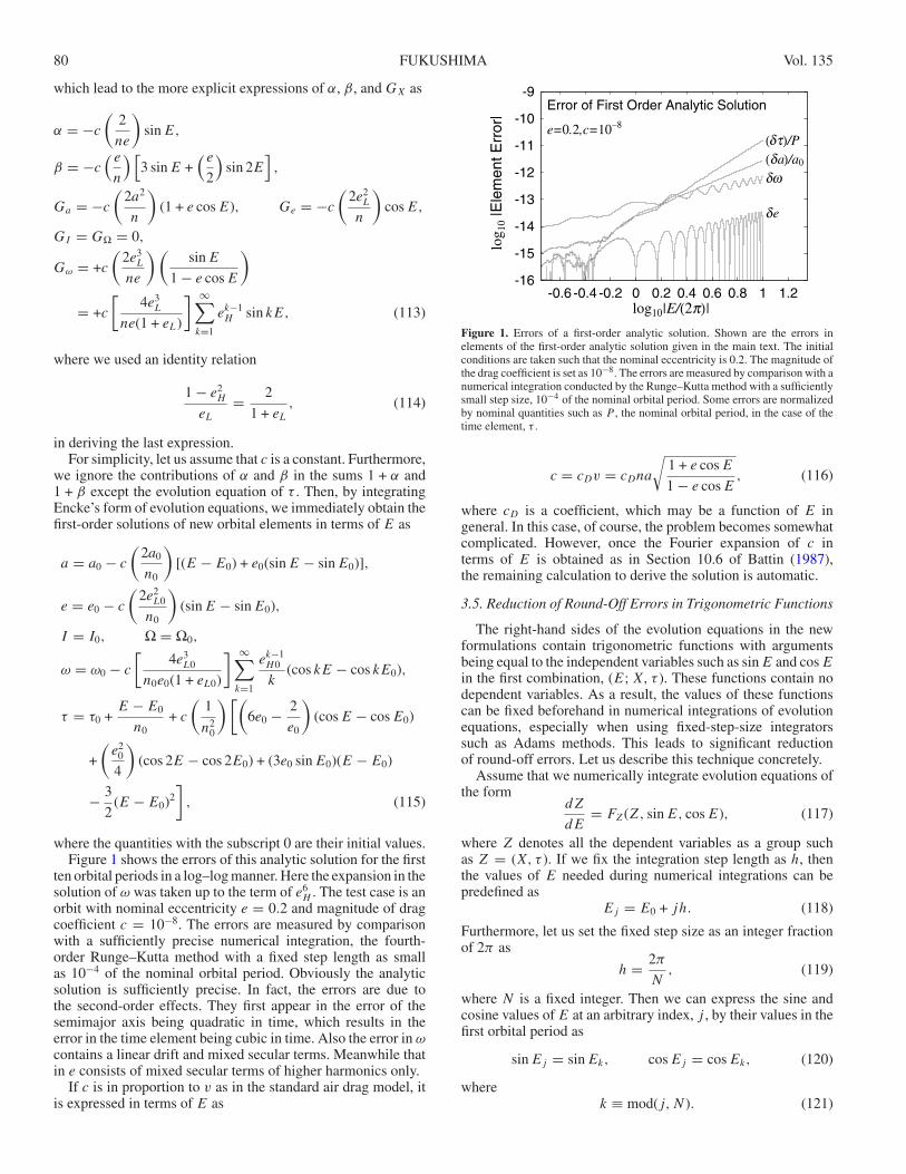
where the quantities with the subscript 0 are their initial values.Figure 1 shows the errors of this analytic solution for the first

ten orbital periods in a log–log manner. Here the expansion in thesolution of ω was taken up to the term of e6

H . The test case is anorbit with nominal eccentricity e = 0.2 and magnitude of dragcoefficient c = 10−8. The errors are measured by comparisonwith a sufficiently precise numerical integration, the fourth-order Runge–Kutta method with a fixed step length as smallas 10−4 of the nominal orbital period. Obviously the analyticsolution is sufficiently precise. In fact, the errors are due tothe second-order effects. They first appear in the error of thesemimajor axis being quadratic in time, which results in theerror in the time element being cubic in time. Also the error in ωcontains a linear drift and mixed secular terms. Meanwhile thatin e consists of mixed secular terms of higher harmonics only.

If c is in proportion to v as in the standard air drag model, itis expressed in terms of E as

-16

-15

-14

-13

-12

-11

-10

-9

-0.6 -0.4 -0.2 0 0.2 0.4 0.6 0.8 1 1.2

log 1

0 |E

lem

ent E

rror

|

Error of First Order Analytic Solution

e=0.2,c=10−8

(δτ)/P(δa)/a0

δe

δω

log10|E/(2π)|Figure 1. Errors of a first-order analytic solution. Shown are the errors inelements of the first-order analytic solution given in the main text. The initialconditions are taken such that the nominal eccentricity is 0.2. The magnitude ofthe drag coefficient is set as 10−8. The errors are measured by comparison with anumerical integration conducted by the Runge–Kutta method with a sufficientlysmall step size, 10−4 of the nominal orbital period. Some errors are normalizedby nominal quantities such as P , the nominal orbital period, in the case of thetime element, τ .

c = cDv = cDna

√1 + e cos E

1 − e cos E, (116)

where cD is a coefficient, which may be a function of E ingeneral. In this case, of course, the problem becomes somewhatcomplicated. However, once the Fourier expansion of c interms of E is obtained as in Section 10.6 of Battin (1987),the remaining calculation to derive the solution is automatic.

3.5. Reduction of Round-Off Errors in Trigonometric Functions

The right-hand sides of the evolution equations in the newformulations contain trigonometric functions with argumentsbeing equal to the independent variables such as sin E and cos Ein the first combination, (E;X, τ ). These functions contain nodependent variables. As a result, the values of these functionscan be fixed beforehand in numerical integrations of evolutionequations, especially when using fixed-step-size integratorssuch as Adams methods. This leads to significant reductionof round-off errors. Let us describe this technique concretely.

Assume that we numerically integrate evolution equations ofthe form

dZ

dE= FZ(Z, sin E, cos E), (117)

where Z denotes all the dependent variables as a group suchas Z = (X, τ ). If we fix the integration step length as h, thenthe values of E needed during numerical integrations can bepredefined as

Ej = E0 + jh. (118)

Furthermore, let us set the fixed step size as an integer fractionof 2π as

h = 2π

N, (119)

where N is a fixed integer. Then we can express the sine andcosine values of E at an arbitrary index, j , by their values in thefirst orbital period as

sin Ej = sin Ek, cos Ej = cos Ek, (120)

wherek ≡ mod(j,N ). (121)

No. 1, 2008 AN ORBITAL ELEMENT FORMULATION 81

-16

-15

-14

-13

-12

-11

-10

-9

-8

-2 -1 0 1 2 3 4 5

log 1

0 |δ

ω |

RK4, ∆E=2−10π

e=0.2,c=10−3

No Care

Prefixed

log10|E/(2π)|

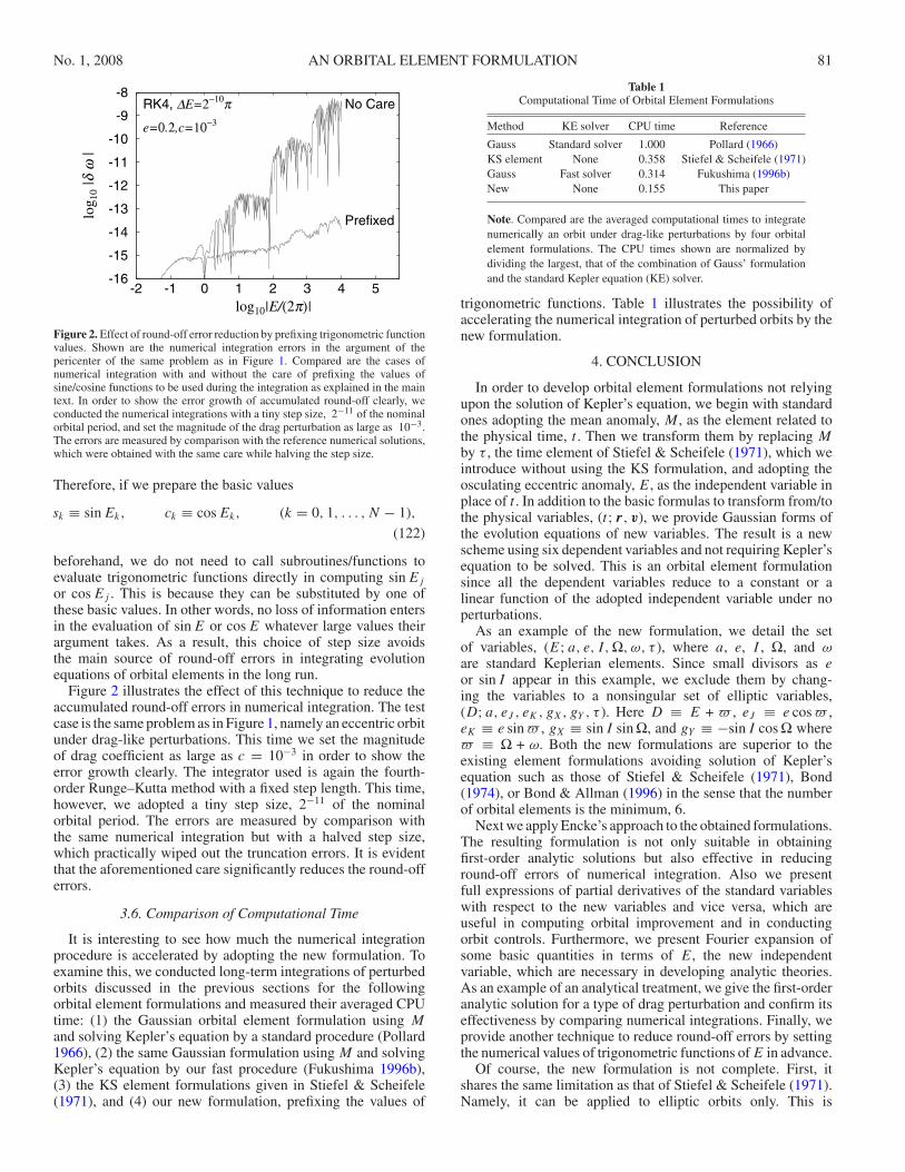
Figure 2. Effect of round-off error reduction by prefixing trigonometric functionvalues. Shown are the numerical integration errors in the argument of thepericenter of the same problem as in Figure 1. Compared are the cases ofnumerical integration with and without the care of prefixing the values ofsine/cosine functions to be used during the integration as explained in the maintext. In order to show the error growth of accumulated round-off clearly, weconducted the numerical integrations with a tiny step size, 2−11 of the nominalorbital period, and set the magnitude of the drag perturbation as large as 10−3.The errors are measured by comparison with the reference numerical solutions,which were obtained with the same care while halving the step size.

Therefore, if we prepare the basic values

sk ≡ sin Ek, ck ≡ cos Ek, (k = 0, 1, . . . , N − 1),

(122)

beforehand, we do not need to call subroutines/functions toevaluate trigonometric functions directly in computing sin Ej

or cos Ej . This is because they can be substituted by one ofthese basic values. In other words, no loss of information entersin the evaluation of sin E or cos E whatever large values theirargument takes. As a result, this choice of step size avoidsthe main source of round-off errors in integrating evolutionequations of orbital elements in the long run.

Figure 2 illustrates the effect of this technique to reduce theaccumulated round-off errors in numerical integration. The testcase is the same problem as in Figure 1, namely an eccentric orbitunder drag-like perturbations. This time we set the magnitudeof drag coefficient as large as c = 10−3 in order to show theerror growth clearly. The integrator used is again the fourth-order Runge–Kutta method with a fixed step length. This time,however, we adopted a tiny step size, 2−11 of the nominalorbital period. The errors are measured by comparison withthe same numerical integration but with a halved step size,which practically wiped out the truncation errors. It is evidentthat the aforementioned care significantly reduces the round-offerrors.

3.6. Comparison of Computational Time

It is interesting to see how much the numerical integrationprocedure is accelerated by adopting the new formulation. Toexamine this, we conducted long-term integrations of perturbedorbits discussed in the previous sections for the followingorbital element formulations and measured their averaged CPUtime: (1) the Gaussian orbital element formulation using Mand solving Kepler’s equation by a standard procedure (Pollard1966), (2) the same Gaussian formulation using M and solvingKepler’s equation by our fast procedure (Fukushima 1996b),(3) the KS element formulations given in Stiefel & Scheifele(1971), and (4) our new formulation, prefixing the values of

Table 1Computational Time of Orbital Element Formulations

Method KE solver CPU time Reference

Gauss Standard solver 1.000 Pollard (1966)KS element None 0.358 Stiefel & Scheifele (1971)Gauss Fast solver 0.314 Fukushima (1996b)New None 0.155 This paper

Note. Compared are the averaged computational times to integratenumerically an orbit under drag-like perturbations by four orbitalelement formulations. The CPU times shown are normalized bydividing the largest, that of the combination of Gauss’ formulationand the standard Kepler equation (KE) solver.

trigonometric functions. Table 1 illustrates the possibility ofaccelerating the numerical integration of perturbed orbits by thenew formulation.

4. CONCLUSION

In order to develop orbital element formulations not relyingupon the solution of Kepler’s equation, we begin with standardones adopting the mean anomaly, M , as the element related tothe physical time, t . Then we transform them by replacing Mby τ , the time element of Stiefel & Scheifele (1971), which weintroduce without using the KS formulation, and adopting theosculating eccentric anomaly, E, as the independent variable inplace of t . In addition to the basic formulas to transform from/tothe physical variables, (t; r, v), we provide Gaussian forms ofthe evolution equations of new variables. The result is a newscheme using six dependent variables and not requiring Kepler’sequation to be solved. This is an orbital element formulationsince all the dependent variables reduce to a constant or alinear function of the adopted independent variable under noperturbations.

As an example of the new formulation, we detail the setof variables, (E; a, e, I, Ω, ω, τ ), where a, e, I , Ω, and ωare standard Keplerian elements. Since small divisors as eor sin I appear in this example, we exclude them by chang-ing the variables to a nonsingular set of elliptic variables,(D; a, eJ , eK, gX, gY , τ ). Here D ≡ E + , eJ ≡ e cos ,eK ≡ e sin , gX ≡ sin I sin Ω, and gY ≡ −sin I cos Ω where ≡ Ω + ω. Both the new formulations are superior to theexisting element formulations avoiding solution of Kepler’sequation such as those of Stiefel & Scheifele (1971), Bond(1974), or Bond & Allman (1996) in the sense that the numberof orbital elements is the minimum, 6.

Next we apply Encke’s approach to the obtained formulations.The resulting formulation is not only suitable in obtainingfirst-order analytic solutions but also effective in reducinground-off errors of numerical integration. Also we presentfull expressions of partial derivatives of the standard variableswith respect to the new variables and vice versa, which areuseful in computing orbital improvement and in conductingorbit controls. Furthermore, we present Fourier expansion ofsome basic quantities in terms of E, the new independentvariable, which are necessary in developing analytic theories.As an example of an analytical treatment, we give the first-orderanalytic solution for a type of drag perturbation and confirm itseffectiveness by comparing numerical integrations. Finally, weprovide another technique to reduce round-off errors by settingthe numerical values of trigonometric functions of E in advance.

Of course, the new formulation is not complete. First, itshares the same limitation as that of Stiefel & Scheifele (1971).Namely, it can be applied to elliptic orbits only. This is

82 FUKUSHIMA Vol. 135

because we assume that the quantity J , which is the doubleof negative Kepler energy, is positive in defining E and τ . Inorder to universalize the current formulations, at least we need auniversal extension of E and M , which is not available yet in theliterature. Another weak point is that no elaborated treatmentsuch as the Lagrangian formalism or the Hamilton–Jacobiapproach is found for the current formulation. As long as we aredealing with first-order perturbation theories, there will be nolarge difference. However, if we go beyond, the availability ofsuch a systematic treatise would make a tremendous differencein deriving high precision solutions. All of these are openproblems and are well worth addressing.

We acknowledge Dr. J. E. Chambers for reviewing themanuscript and suggesting improvements.

REFERENCES

Battin, R. H. 1987, An Introduction to the Mathematics and Methods ofAstrodynamics (New York: AIAA)

Bond, V. R. 1974, Celest. Mech., 10, 303Bond, V. R., & Allman, M. C. 1996, Modern Astrodynamics (Princeton, NJ:

Princeton Univ. Press)Broucke, R., & Cefola, P. 1972, Celest. Mech., 5, 303Brouwer, D., & Clemence, G. M. 1961, Methods of Celestial Mechanics

(New York: Academic)Burdet, C. A. 1967, Z. Angew. Math. Phys., 18, 434Burdet, C. A. 1968, Z. Angew. Math. Phys., 19, 345Colwell, P. 1993, Solving Kepler’s Equation over Three Centuries (Richmond,

VA: Willmann-Bell)Danby, J. M. A. 1988, Fundamentals of Celestial Mechanics (2nd ed.;

Richmond, VA: Willmann-Bell)Feinstein, S. A., & McLaughlin, C. A. 2007, Celest. Mech. Dyn. Astron., 96,

49Fukushima, T. 1996a, AJ, 112, 1263Fukushima, T. 1996b, Celest. Mech. Dyn. Astron., 66, 309Fukushima, T. 1999, Celest. Mech. Dyn. Astron., 75, 201Kustaanheimo, P., & Stiefel, E. L. 1965, J. Reine Angew. Math., 218, 204Pollard, H. 1966, Mathematical Introduction to Celestial Mechanics (New

York: Prentice-Hall)Roy, A. E. 2002, Orbital Motion (4th ed.; Bristol: Adam Hilger)Sperling, H. 1961, Am. Rocket. Soc. J., 31, 1032Stiefel, E. L., & Scheifele, G. 1971, Linear and Regular Celestial Mechanics

(New York: Springer)