Universite Pierre et Marie Curie et

ONERA

Fonctions de base pour la resolution d’equation de transportBasis functions for solving the transport equation

Rapport de fin d’etudes

de

Christina Yassouridis

Directeur de memoire: Eric SavinDate de remise: 31. Aout 2011

Contents

1 Presentation of ONERA 4

1.1 Internship . . . . . . . . . . . . . . . . . . . . . . . . . . . . . . . . . . . . . . . . 5

2 Theory 5

2.1 Physical model . . . . . . . . . . . . . . . . . . . . . . . . . . . . . . . . . . . . . 5

2.1.1 Energy density . . . . . . . . . . . . . . . . . . . . . . . . . . . . . . . . . 5

2.1.2 Space-time energy density and flux . . . . . . . . . . . . . . . . . . . . . . 6

2.1.3 Assumptions . . . . . . . . . . . . . . . . . . . . . . . . . . . . . . . . . . 6

2.1.4 Boundary conditions . . . . . . . . . . . . . . . . . . . . . . . . . . . . . . 7

2.1.5 Interfaces . . . . . . . . . . . . . . . . . . . . . . . . . . . . . . . . . . . . 7

2.1.6 Wave transmission and reflection at interfaces . . . . . . . . . . . . . . . . 8

2.1.6.1 Snell Descartes Law . . . . . . . . . . . . . . . . . . . . . . . . . 8

2.1.6.2 Critical angle for transmission . . . . . . . . . . . . . . . . . . . 8

2.1.6.3 Critical angle for reflection . . . . . . . . . . . . . . . . . . . . . 8

2.1.6.4 Reflection/transmission coefficients . . . . . . . . . . . . . . . . 9

2.2 Discontinuous Galerkin method (DG) . . . . . . . . . . . . . . . . . . . . . . . . 10

2.2.1 Variational formulation . . . . . . . . . . . . . . . . . . . . . . . . . . . . 10

2.2.2 Discretization . . . . . . . . . . . . . . . . . . . . . . . . . . . . . . . . . . 10

2.3 Time integration . . . . . . . . . . . . . . . . . . . . . . . . . . . . . . . . . . . . 12

2.3.1 Runge-Kutta- and SSP- methods . . . . . . . . . . . . . . . . . . . . . . . 13

3 Application 14

3.1 Discontinuous Galerkin method . . . . . . . . . . . . . . . . . . . . . . . . . . . . 14

3.1.1 Variational formulation . . . . . . . . . . . . . . . . . . . . . . . . . . . . 14

3.1.2 Discretization . . . . . . . . . . . . . . . . . . . . . . . . . . . . . . . . . . 15

3.2 Time integration . . . . . . . . . . . . . . . . . . . . . . . . . . . . . . . . . . . . 17

3.2.1 Initial condition . . . . . . . . . . . . . . . . . . . . . . . . . . . . . . . . 17

3.3 Finding the right basis functions . . . . . . . . . . . . . . . . . . . . . . . . . . . 17

3.3.1 Fourier polynomials . . . . . . . . . . . . . . . . . . . . . . . . . . . . . . 19

3.3.2 Results . . . . . . . . . . . . . . . . . . . . . . . . . . . . . . . . . . . . . 20

3.3.3 Problems . . . . . . . . . . . . . . . . . . . . . . . . . . . . . . . . . . . . 21

3.3.3.1 Negativity . . . . . . . . . . . . . . . . . . . . . . . . . . . . . . 21

3.3.3.2 Dispersion . . . . . . . . . . . . . . . . . . . . . . . . . . . . . . 21

3.3.4 Solutions . . . . . . . . . . . . . . . . . . . . . . . . . . . . . . . . . . . . 23

2

3.3.4.1 Nurbs . . . . . . . . . . . . . . . . . . . . . . . . . . . . . . . . . 23

3.3.4.2 Fourier-Collocation method . . . . . . . . . . . . . . . . . . . . . 26

4 Conclusion 28

5 Outlook 28

3

1 Presentation of ONERA

Founded by the French government in 1946, ONERA (Office National d’Etudes et de RecherchesAerospatiales) is a public aerospace research institution with commercial and industrial char-acter, building a bridge between government, science and industry. It combines fundamentalwith applied research with the result of computation codes, methods, tools, technologies ormaterials.

The missions of ONERA are the following:

• Aeronautic research

• Commercializing the research by national and European industry

• Construct and operate experimental facilities

• Supply the industry with research results

• Supply the government with technical analyzes

• Train new researchers and engineers

The company consists of eight major centers and about 2,000 employees, including 1,500 scien-tists, engineers and technicians, 259 of them being doctoral students. It works with a budget of227 Million Euros financed to 60% through projects for industry and agencies and to 40% bythe French government.Not only simulation tools but also experimentations are conducted at different stages to developmechanisms and verify calculations.Therefore Onera possesses lab testing facilities for basic research as well as different wind tunnelsin Meudon, Fauga-Mauzac and Modane-Avrieux. The aerospace lab is divided into 16 scientificdepartments, grouped into four namely:

Fluid Mechanics and Energetics

Physics

Materials and Structures

Information Processing and Systems

Each scientific field is subdivided into 4 departments. One subdepartment of the Materialsand Structures branch is the DADS (Department of Aeroelasticity and Structural Dynamics).Its task is the analysis of static and dynamical behavior of structures in their environment.Subjects of research are mechanical design, structural dynamics and vibration, aeroelasticityand vibroacoustics. Its application contains all kinds of aeronautic and space products such asaircrafts, helicopters, turbine engines, missiles or satellites.

4

1.1 Internship

The internship was carried out in the department DADS under the supervision of EricSavin working in the research area of high precision methods for linear and non-linear wavepropagation systems. Stiffened plates, shells and beams are often used as structural componentsfor ground, underwater or aerospace vehicles. If they undergo shocks, vibrations are generated.Therefore they imply the need of vibro-acoustic response characteristics to high frequencymechanical or acoustical excitations. The characteristics are in the form of energetic wavestravelling through the structures. If the material is heterogeneous, i.e. at material changes ortwo attached plates, multiple reflection and scattering occurs at the interfaces between thesubstructures.

The mathematical model describing these phenomena focuses on the energy density associatedto the waves by using Wigner measures. It is based on the Liouville transport equation firstdeveloped to describe how light energy propagates through a turbulent atmosphere [10]. Thetheory was later extended for other types of waves in a randomly heterogeneous medium. Itresults in radiative transfer equations for the angularly resolved energy density in elastic media.The angular resolution is needed to describe how a wave with wave vector k′ at position xcan be scattered into another direction with wave vector k. Thus not only a physical space forx ∈ O ⊂ Rd is considered but also a spherical space for the wave vectors k ∈ Rd, where d = 1, 2or 3 is the physical space dimension. The numerical method used to solve the radiative transferequations is the discontinuous Galerkin method. This method, which is based on a variationalformulation, requires basis functions in phase space O×Rd of which linear combinations describethe energy density of a wave at position x and in the direction k. For each of these variables adifferent type of basis functions can be defined which together form the full solution space.

Finding adequate basis functions for the propagation direction is however a challenging problem,that has been investigated for quite a while ([11],[2]). So far Fourier, Lagrange and Jacobipolynomials were tested but all of them had unwanted effects such as rays, dispersion problemsor negativity. The task of my internship was to test different sets of basis functions in orderto improve the result. The functions I was working with were Non Uniform Rational B-Splines(NURBS) and Fourier collocation polynomials.

2 Theory

2.1 Physical model

2.1.1 Energy density

Let ω(t, x, k) be the energy density in phase space at time t of a scalar wave field satisfying astandard scalar wave equation. For sound speeds varying randomly at the same length scalesas the wave lengths, it satisfies in the limit of vanishing wave lengths the following radiativetransfer equation [10]:

∂tω(t, x, k) +Hω(t, x, k) =

∫Rdσ(x, k, k′)

(ω(t, x, k′)− ω(t, x, k)

)dk′ (1)

where H stands for the Hamilton operator:

Hf = ∇kλ(x, k)∇xf(t, x, k)−∇xλ(x, k)∇kf(t, x, k) , (2)

5

λ(x, k) is the frequency at x of the wave vector k, and σ(x, k, k′) is a differential scatteringcross-section. It gives the rate of change of an energy ray travelling in the direction of k′ intoanother ray k due to its scattering on the random perturbations of the sound speed. Here anenergy ray corresponds to the trajectory of the energy density in physical space oriented by thewave vector k. It is also the projection in physical space of the bicharacteristic curves associatedto the wave equation.

In this work an heterogeneous, elastic medium embedded in the open domain O ∈ Rd is consid-ered. Because waves are now vector waves with possibly M different polarizations (the directionsof wave motion), M different energy propagation modes are now coupled through the followingmultigroup radiative transfer equations [11]:

∂tωα(t, x, k) +Hαωα(t, x, k) =

M∑β=1

∫Rdσαβ(x, k, k′)

(ωβ(t, x, k′)− ωα(t, x, k)

)dk′ (3)

with:

Hαf = ∇kλα(x, k)∇xf(t, x, k)−∇xλα(x, k)∇kf(t, x, k) for 1 ≤ α ≤M , (4)

and σαβ is the rate of conversion of an energy ray β in direction k′ to an energy ray α in directionk.

In an isotropic elastic medium, three wave modes α coexist: α = P, SV or SH for the compres-sional, shear or transverse shear waves, respectively. The eigenfrequency of the wave mode α isgiven by λα(x, k) = cα(x)|k|, where cα(x) is the energy group velocity and |k| is the wavenumber.

2.1.2 Space-time energy density and flux

The total energy density ε at a point x and time t is recovered by summing the phase-spaceenergy densities over all directions and for all waves types. This leads to:

ε(x, t) =1

2

M∑α=1

∫Rdωα(t, x, k)dk . (5)

The total energy flux density π is given by:

π(x, t) =1

2

M∑α=1

∫Rdcα(x)ωα(t, x, k)kdk , (6)

where k := k|k| ∈ Sd−1, the unit sphere of Rd.

2.1.3 Assumptions

In order to facilitate the subsequent computation of the numerical solutions of the radiativetransfer equations, the following assumptions are made:

• Constant wavenumberThe wavenumber |k| is taken to be constant for all types of waves. Then ωα(t, x, k) =ωα(t, x, |k|k) ≡ ωα(t, x, k) so that the domain of k reduces to the unit sphere Sd−1.

6

• Phase spaceWith D being a bounded subset of O the computational phase space X is defined byX = D× Sd−1.

• Deterministic mediumThe medium is considered to be deterministic (no random inhomogeneities). This leads tothe scattering cross-sections being zero:

Σα(x, k) =

M∑β=1

∫Rdσαβ(x, k, k′)dk′ = 0 .

• Constant velocityThe velocity cα(x) is assumed to be constant so that the Hamilton operator (4) reducesto the first term.

2.1.4 Boundary conditions

Let:

Γ± = (x, k) ∈ ∂D× Sd−1;±k · n(x) > 0 ,

where n(x) is the outward unit normal to the boundary ∂D. At the inward boundary Γ− either asource term gα(t, x, k) is considered, or an incident wave of mode β in direction k′ is reflected intoa wave of mode α in direction k with the rate (a reflection coefficient) ραβ(x, k, k′). To be more

exact, ραβ(x, k, k′) describes how the outward energy flux density cβωβ(t, x, k′)k′ (see Eq. (6))

such that k′ ·n(x) > 0 is reflected into the inward energy flux cαωα(t, x, k)k such that k ·n(x) < 0,with a possible mode conversion β → α. The boundary condition for the energy fluxes at Γ−thus reads:

−cαωα(t, x, k)k ·n(x) = gα(t, x, k) +M∑β=1

∫k·n(x)>0

ραβ(x, k, k′)cβωβ(t, x, k′)k′ ·n(x)dµ(k) , (7)

where µ is the natural measure on the unit sphere Sd−1. In the following example it is assumedthat there is no boundary source, so that the term gα(t, x, k) in equation (7) is zero.

2.1.5 Interfaces

At interfaces between different media the waves are transmitted or reflected. During transmissionthe mode and direction can change, so similarly as in the reflection case a wave of mode β anddirection k′ can be transformed into a wave of mode α and direction k. The transmission angleand transmission coefficient θαβ are calculated by the Snell-Descartes law described in the nextsection. Let ΣD be a regular interface between the media, oriented by its unit normal nD(x)pointing from the left to the right. The left side of ΣD is labelled with a minus sign − andits right side by a plus sign +. For a function f(x) defined on both sides of ΣD, let its tracesbe: f±(x) = limh→0+ f(x ± hnD(x)). c+

β and c−α are the wave celerities of the modes β and α,

respectively, on both sides of the interface. Then the outgoing flux term (k · nD(x) > 0) at that

7

interface is expressed by:

c+αω

+α (t, x, k)k · nD(x) =

M∑β=1

(∫k′·nD(x)>0

τ−αβ(x, k, k′)c−β ω−β (t, x, k′)k′ · nD(x)dµ(k′)

−∫k′·nD(x)<0

ρ+αβ(x, k, k′)c+

β ω+β (t, x, k′)k′ · nD(x)dµ(k′)

),

(8)

and the incoming (k · nD < 0) flux by:

c−αω−α (t, x, k)k · nD(x) =

M∑β=1

(∫k′·nD(x)<0

τ+αβ(x, k, k′)c+

β ω+β (t, x, k′)k′ · nD(x)dµ(k′)

−∫k′·nD(x)>0

ρ−αβ(x, k, k′)c−β ω−β (t, x, k′)k′ · nD(x)dµ(k′)

).

(9)

2.1.6 Wave transmission and reflection at interfaces

2.1.6.1 Snell Descartes Law The direction into which a wave is transmitted or reflectedwhen passing from a medium into another with different material parameters can be calculatedby the Snell-Descartes law. This law is based on the fact that the breaking of the wave directionis caused by different propagation velocities in different materials. It describes the relationshipbetween the incident and emergent angles and states that the following equation holds:

sin θi

sin θ−+αβ

=c+β

c−α,

where θi is the incidence angle of a ray in material + for instance, and θ−+αβ is the transmission

angle of a ray passing from material + in mode β into material − with mode α.

2.1.6.2 Critical angle for transmission If the incident angle increases, the transmissionangle increases as well, so that at a certain threshold the ray is parallel to the tangent of theinterface at the point x. This angle is called the critical angle and is defined by:

θc = arcsin

(c+β

c−α

).

Fig. (1) clarifies this situation. Critical incidences are neglected in our problem because we lack atheoretical model for the transmission process of the energy densities in this case. For incidenceangles greater than the critical one the transmission coefficient is zero because they correspondto surface waves of vanishing energy.

2.1.6.3 Critical angle for reflection The same situation of critical incidence during trans-mission arises for reflection when mode conversion occurs. Without mode conversion the reflectedangle is the same as the incidence angle what is called specular reflection. By Snell-Descarteslaw the following relationship holds:

sin θi

sin θ++αβ

=c+β

c+α,

8

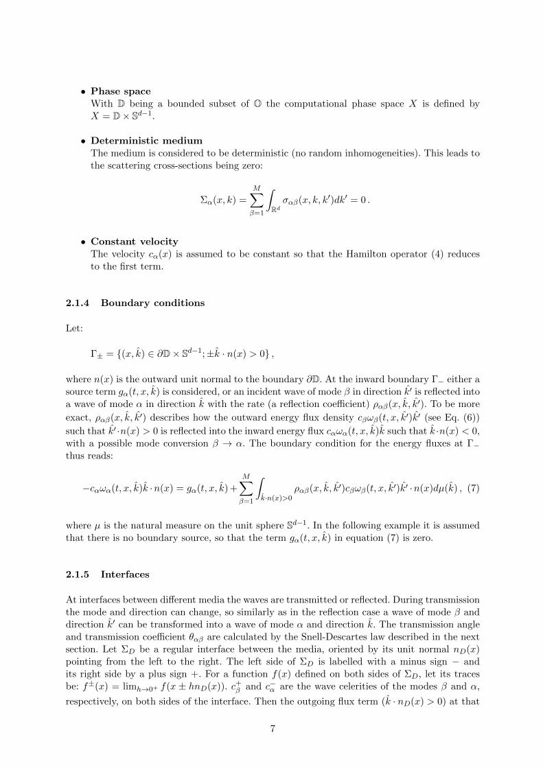
Figure 1: Reflection/transmission of waves at a straight interface. The ray with incident angleθ1 is transmitted into ray with outgoing angle θ2. With increasing θ1 the transmission angle θ2

increases as well until θ1 reaches the critical angle θc where the emerging ray glides along theboundary. θ3 shows a speculare reflection.

θ++αβ being now the reflection angle of a ray in mode β being converted into mode α on the +

side of the interface. The corresponding critical angle is:

θc = arcsin

(c+β

c+α

).

2.1.6.4 Reflection/transmission coefficients The reflection and transmission coefficientsin equations (8) and (9) are given by:

ρ±αβ(x, k, k′)dµ(k) = R±αβ(x, k′)δ(k − R±αβ(k′)) ,

τ±αβ(x, k, k′)dµ(k) = T±αβ(x, k′)δ(k − T±αβ(k′)) ,

with positive smooth functions R±αβ(x, k′) and T±αβ(x, k′).

δ is the Dirac measure so that for any function f(k):⟨f, δ(k − k′)

⟩=

∫Sd−1

δ(k − k′)f(k) dµ(k) = f(k′) .

Finally, R±αβ(k′) and T±αβ(k′) are the reflection and transmission directions corresponding to the

reflection/transmission angles θ±αβ introduced above, for the incidence angle of k′.

9

2.2 Discontinuous Galerkin method (DG)

DG is a class of numerical methods for solving partial differential equations with possible dis-continuous solutions. It combines the finite element and the finite volume method. This meansthat the solution is represented within each element as a polynomial approximation with aninter-cell communication at cells sharing a common face. The inter-element convection termsare resolved with upwinded numerical flux formulas and the elementwise defined polynomialsare independent of the solutions in other cells.Such as the finite element method, the discontinuous Galerkin method is based on a variationalformulation. Its theory is explained in the following on a simple time-independent advection-reaction equation [6].Let Ω ∈ Rd be a bounded convex domain. The passive advection of a scalar field u(x) that iscarried along by a flow of speed c(x) ∈ [W 1,∞(Ω)]d (W k,p = u ∈ Lp(Ω);Dα ∈ Lp(Ω); |α| ≤ k)with a source term f ∈ L2(Ω) is described by:

u+ c · ∇u = f u ∈ Ω

u = 0 u ∈ Γ−(10)

where Γ is the boundary of Ω and Γ± are the incoming and outgoing flux parts of the boundarydefined by Γ± = x ∈ Γ; ±c(x) · n(x) > 0 with the outward pointing normal vector n(x).

2.2.1 Variational formulation

To obtain the variational formulation, Eq. (10) is multiplied by an adequate test function ψ andintegrated over the domain Ω. If the functions ψ and u are continuous throughout the elementsthe bilinear form α(u, ψ) becomes:

α(u, ψ) =

∫ΩuψdΩ +

∫Γ[c · n]−uψdσ +

∫Ωc · ∇uψdΩ (11)

with a right hand side:

α(u, ψ) =

∫ΩfψdΩ (12)

[x]± := 12(|x| ± x) denotes the positive and negative part of a variable x.

Proof:∫Ωc · ∇uψdΩ =

∫Γ[c · n]+uψdσ −

∫Ωuc · ∇ψdΩ =

∫Γ[c · n]+uψdσ −

∫Γc · nuψdσ +

∫Ωc · ∇uψdΩ =∫

Γ[c · n]−uψdσ +

∫Ωc · ∇uψdΩ

2.2.2 Discretization

The domain Ω is then discretized into a set of non-overlapping subdomains Ωi with Ω =⋃

Ωi.The boundaries or interfaces of a cell Ωi are denoted by F ∈ ∂Ωi where ∂Ωi is the total boundaryof cell Ωi and the interior interfaces are denoted by F int if F ∩ Γ = ∅. At F int discontinuitiesmight occur, so that the test function ψ and the function u are assumed to lie in the brokenSobolev space:

Gkh = v ∈ L2(Ω) ∀Ωi ∈ Ω v|Ωi ∈ P k

10

P k is usually a polynomial of degree k.To clarify this relationship functions in the broken Sobolev space are denoted by ψh and uh.In between two different cells, jumps and mean values are defined by: [|u|] := (u− − u+) andu := 1

2(u− + u+) with u±(x) = limh→0+ u(x± hnF (x)) and where nF is the outward pointingnormal at an interface F .

Regarding the equalitiy

[|u2h|] = [|uh|]uh (13)

the broken bilinear αh(uh, ψh) form becomes:

αh(uh, ψh) =∑i

(∫Ωi

uhψhdΩi +

∫Ωi

c · ∇uhψhdΩi

)−∑i

∑F int∈∂Ωi

∫Fc · nF [|uh|]ψhdσ +

∑F∈Γ

∫F

[c · nF ]−uhψhdσ

(14)

Proof:L2-coercivity αh(uh, uh) ≥ c‖uh‖2 with a positive constant c is a neccessary condition for theexistence of a solution. If the continuous bilinear form α(u, φ) was used as broken bilinear form,then α(uh, φh) would contain a term that could harm the L2-coercivity and must therefore besubtracted.

a(uh, uh) =∑i

(∫Ωi

uhuhdΩi +

∫Ωi

c · ∇uhuhdΩi

)+∑F∈Γ

∫F

[c · nF ]−uhuhdσ =

∑i

∫Ωi

u2hdΩi +

∑i

∑F int∈∂Ωi

1

2

∫F

[|c · nFu2h|]dσ +

∑F∈Γ

1

2

∫Fc · nFu2

hdσ −∑i

1

2

∫Ωi

∇ · cu2hdΩi+

∑F∈Γ

1

2

∫F

(|c · nF | − c · nF )u2hdσ =∫

Ω(1− 1

2∇ · c)u2

hdΩ +

∫Γ

1

2|c · n|u2

hdσ +∑i

∑F int∈∂Ωi

[|c · nFu2h|]dσ

Let us assume that (1− 12∇ · c) ≥ 0 in Ω. Then the coercivity holds if the last term is positive.

Since its sign is not known it is subtracted from the bilinear form what leads with the egality ofEq. (13) to the broken bilinear form αh(uh, ψh) of Eq. (14).

The jumps at interior interfaces are now penalized by a penalization function which is added tothe bilinear form. It takes the form:

p∑i

∑F int∈∂Ωi

∫F|c · nF |[|uh|][|ψh|]dσ (15)

11

with a positive constant p that can depend on x. The final broken bilinear form reads:

αh(uh, ψh) =∑i

(∫Ωi

uhψhdΩi +

∫Ωi

c · ∇uhψhdΩi

)−∑i

∑F int∈∂Ωi

c · nF [|uh|]ψhdσ +∑F∈Γ

∫F

[c · nF ]−uhψhdσ +p

2

∑i

∑F int∈∂Ωi

∫F

|c · nF |[|uh|][|ψh|]dσ =

∑i

(∫Ωi

uhψhdΩi −∫

Ωi

c · ∇ψhuhdΩi

)+

∑i

∑F int∈∂Ωi

∫F

c · nF uh[|ψh|]dσ +∑F∈Γ

∫F

(c · nF )+uhψhdσ +p

2

∑i

∑F int∈∂Ωi

∫F

|c · nF |[|uh|][|ψh|]dΩi

(16)

The local formulation for this equation admits to define the fluxes as a function of an interface F .To generalize the notation a test function ψh with ψh = q1Ωi

is chosen where q is an arbitrary polynomialand 1Ωi the indication function defined by:

1Ωi(x) =

1 if x ∈ Ωi

0 else.

A common way to write Eq. (16) is:

∑i

(∫Ωi

uhqhdΩi −∫

Ωi

uhc · ∇qhdΩi

)+∑F

∫F

Φ(F )(uh)qhdσ (17)

Φ(F ) is a up-winded numerical flux function depending on the left and right traces of u.In the above case it represents the standard Lax-Friedrich flux defined by:

Φ(F ) =

(c · nF )u(x)+ p(x)

2 |c · nF |[|u(x)|] if F ∈ F int

(c · n)+u(x) else

For p = 0 the fluxes are centered and p = 1 leads to upwind fluxes.

Let Gih be the set of functions forming a basis of Ωi, i.e. Gih = ψil : Ωi → R; l = 1 . . . L.Then the same functions are used as test functions so that the numerical solution at element i, uih isformed by a linear combination of the basis functions of Gih

uih =

L∑l=1

qlψil ψil ∈ Gih

Plugging the above equality into Eq. (17), it becomes a quadratic, ordinary differential equation systemof the form:

Aiuih = 0 (18)

Ai is the matrix containing the integrals of the basis functions over the elements Ωi. It is not closerdefined here but will be explained in the next section for our specific model.

2.3 Time integration

Once the system in Eq. (32) is set up, the integration in time is performed. The most common methodtherefore is the Runge-Kutta-method.

12

2.3.1 Runge-Kutta- and SSP- methods

Consider the hyperbolic conservation law:

∂tu+ ∂xf(u) = 0 (19)

The method of lines first discretizes ∂xf(u) in space, usually by the finite element method or in discontin-uous cases by the DG-method, resulting in a numerical approximation D(u) = −∂xf(u) + 0(4xk) whereD(u) does not depend on spatial derivatives anymore.0(4xk) is the approximation error of the discretization scheme with mesh size 4x and order k.

Once the space discretization is found, the time integration to solve ∂tu = −D(u) is preformed by aRunge-Kutta-method. An explicit Runge-Kutta-method of order 1 is the forward Euler-method (FE-method) given by:

un+1 = un +4tD(un) (20)

The method is said to be strongly stable if:

‖un+1‖ ≤ ‖un‖ ∀n ≥ 0 (21)

under a certain norm ‖.‖.

The FE-method is strongly stable for a sufficiently small time step 4t ≤ 4tCFL where 4tCFL is theCourant-Friedrich-Levy number. If the problem has a discontinuous solution though (as often for hyper-bolic problems) strong stability is not preserved. This induces the need of stability preserving methodsfor higher orders.

Strong stability preserving methods (SSP)A stronger measure than linear stability is required. Some form of nonlinear stability property must beintroduced i.e. by requiring that the total variation of the numerical solution does not increase in time(total variation diminishing property) [13]. This is of special interest when the solution exhibits shock-like or other non smooth behaviors. Methods that make use of this property are SSP-methods. Assumingthat the first order forward Euler time discretization is strongly stable when the time step 4t is suitablyrestricted, they try to find a higher order time discretization that maintains the stability maybe under amore restricted time step.

The total variation diminishing property is defined by:

TV (un+1) ≤ TV (un) with TV (un) :=∑j

|unj+1 − unj | (22)

where uj are the the points derived from the spatial disretization.

A general m-stage Runge-Kutta-method for an equation ∂tu+D(u) = 0 is of the form [3]:

u0 = un

ui =

i−1∑k=0

(αi,ku

k +4tβi,kD(uk))

i = 1 . . .m

un+1 = um

(23)

with coefficients αi,k ≥ 0 and βi,k and where αi,k = 0 only if βi,k = 0.

For consistency reasons∑i−1k=0 αi,k = 1 for i = 1 . . .m .

If the forward Euler-method Eq. (20) is strongly stable under the TV -norm defined in Eq. (22), then theRunge-Kutta-method (23) with βi,k ≥ 0 is SSP under the restriction

4t ≤ c4 tCFL with c = minαikβik

. (24)

(see [9]).

Because a very small time step leads to a long calculation time, much of the research in the area of SSP-methods concentrates on finding optimal SSP-schemes in the sense of Runge-Kutta-schemes for which cis a maximum under the given constraints placed on the αik and βik.

13

3 Application

In the following the theory is applied to our model equation by using the DG-method for the spacediscretization and SSP-methods of order 2 and 3 for the time integration.

3.1 Discontinuous Galerkin method

Eq. (3) was simplified under assumption of a zero right hand so that the equation to investigate is thefollowing:

ωα(t, x, k) : ([0 T ]× D× Sd−1)→ R

∂tωα(t, x, k) +Hαωα(t, x, k) = 0 (25)

With the assumptions of 2.1.3 it becomes:

∂tωα(t, x, k) +∇kλα(x, k)∇xω(t, x, k) = 0 (26)

3.1.1 Variational formulation

For the continuous problem the solution space is defined by:

V = v ∈ H1(X); v|Γ± ∈ L2µ(Γ±)

withL2µ(Γ±) = v : Γ± → R;

∫Γ±|v(X)|2k · n(x)dµ(k)dγ(x) <∞ and

Γ± = (x, k) ∈ (∂D× Sd−1) : k · n(x)<≥0H1 is the usual Sobolev space, γ is the surface measure of Γ± and X is the phase space X = D × Sd−1

from section 2.1.3.

Because of the possible discontinuities the domain D is divided into non-overlapping subdomains Di.γD is either an interface between two subdomains or a boundary part if ∂Di ∩ Γ± 6= ∅.wi describes the corresponding discretization of X so that wi ∈ (Di × Sd−1) and w±D is its left and right

boundary w±D ∈ ((γD × Sd−1);±k · nD(x) > 0) with the interface normal nD. With these notations thebroken Sobolev space reads:

Vh = v ∈ L2(X); v|wi∈ V (wi) ∀wi ∈ X

With a test function v(x, k) ∈ Vh the elementwise bilinear form is defined by:

α(ωα, v) =∫wi

v(x, k)∂tωα(t, x, k)dµ(k)dx−∫wi

cαk · ∇xv(x, k)ωα(t, x, k)dµ(k)dx

+

∫γD×Sd−1

v(x, k)F (c−αω−α , c

+αω

+α ) · nD(x)dµ(k)dγ(x)

(27)

where the flux term is defined by:

14

∫γD×Sd−1

v(x, k)F (c−αω−α , c

+αω

+α ) · nD(x)dµ(k)dγ(x) =∫

w+D

v(x, k)ω−α (t, x, k)c−α (x)k · nD(x)dµ(k)dγ(x)+

M∑β=1

∫w−D

v(x, k)

(∫k′·nD(x)<0

τ+αβ(x, k, k′)c+β (x)ω+

β (t, x, k′)k′ · nD(x)dµ(k′)−

∫k′·nD(x)>0

ρ−αβ(x, k, k′)c−β (x)ω−β (t, x, k′)k′ · nD(x)dµ(k′)

)dµ(k)dγ(x)

(28)

Proof:

∫wi

v(x, k)∂tωα(t, x, k)dµ(k)dx+

∫wi

∇kλα · ∇xωα(t, x, k)v(x, k)dµ(k)dx =∫wi

v(x, k)∂tωα(t, x, k)dµ(k)dx+

∫wi

cαk · ∇xωα(t, x, k)v(x, k)dµ(k)dx =∫wi

v(x, k)∂tωα(t, x, k)dµ(k)dx−∫wi

cαωα(t, x, k)k · ∇xv(x, k)dµ(k)dx+∫w+

D

k · nDc−αω−α (t, x, k)v(x, k)dµ(k)dγ(x) +

∫w−D

k · nDc+αω+α (t, x, k)v(x, k)dµ(k)dγ(x) =∫

wi

v(x, k)∂tωα(t, x, k)dµ(k)dx−∫wi

cαωα(t, x, k)k · ∇xv(x, k) +

∫w+

D

k · nDc−αω−α (t, x, k)v(x, k)+∫w−D

−|k · nD|c+αω+α (t, x, k)v(x, k) =∫

wi

v(x, k)∂tωα(t, x, k)dµ(k)dx−∫wi

cαωα(t, x, k)k · ∇xv(x, k)dµ(k)dx+

∫w+

D

k · nDc−αω−α (t, x, k)v(x, k)dµ(k)dγ(x) +

M∑β=1

∫w−D

(∫k′·nD(x)<0

τ+αβ(x, k, k′)c+β (x)ω+

β (t, x, k′)k′ · nD(x)dµ(k′)−

∫k′·nD(x)>0

ρ−αβ(x, k, k′)c−β (x)ω−β (t, x, k′)k′ · nD(x)dµ(k′))v(x, k)

)dµ(k)dγ(x)

3.1.2 Discretization

The solution ωα|wi(t, x, k) is a linear combination of basis functions in x and k so that a local

solution ωiα(t, x, k) at element i is given by:

ωiα(t, x, k) =

N−1∑l=0

ξiα,l(t)ψil(x, k) (29)

where ψil(x, k) are local basis functions in Vh for l = 0 . . . N − 1.

The current in each cell is composed by 3 fluxes.

• A transmission part flowing in a neighboring cell without mode conversion.

15

• A reflection part reaching the cell boundary with possible mode conversion.

• A transmission part coming from a neighbor cell with possible mode conversion.

The flux term Eq. (28) is therefore separated into two parts:The reflection and transmission of the current cell i:∫

w+D

v(x, k)ω−α (t, x, k)c−α (x)k · nD(x)dµ(k)dγ(x)+

∫w−D

(∫k′·nD(x)>0

ρ−αβ(x, k, k′)c−β (x)ω−β (t, x, k′)k′ · nD(x)dµ(k′)

)v(x, k)dµ(k)dγ(x)

(30)

and the transmission of a neighboring cell j:∫w−D

(∫k′·nD(x)<0

τ+αβ(t, x, k)c+

β (x)ω+β (t, x, k′)k′ · nD(x)dµ(k′)

)v(x, k)dµ(k)dγ(x) . (31)

If ωiα(t, x, k) is used from Eq. (29) and the same basis functions ψil are used for the test space,then for each cell i = 1 . . . n equation Eq. (27) ends up in a matrix system of the form:

M iξit(t) + Siξi(t) +∑j∈J(i)

Ljξj(t) = 0 ξi(0) = Ξi (32)

where J(i) are the adjacent cells of i and Ξ the vector for the initial condition.

The matrices are:M i = Mass matrix Si = Stiffness matrix Li = Flux matrix.If x ∈ Rd is projected into the unit space x ∈ [−1 1]d by a function Fi with its Jacobian DFi(x)and its determinant Ji(x) = det(DFi(x)) they are given by:

M i(l,m) =

δαβ ⊗∫wi

|Ji(x)|ψl(x, k)ψm(x, k)dµ(k)dx(33)

Biαβ(l,m) =

− δαβ ⊗∫wi

|Ji(x)|ψl(x, k)DF−1i (x)ciαk · ∇xψm(x, k)dµ(k)dx

+ δαβ ⊗∫w+D

Ji(x)ψl(x, k)ψm(x, k)DF−1i ciαk · nD(x)dµ(k)dγ(x)

−∫w−D

Ji(x)ψm(x, k)

(∫DF−1

j k′·nD(x)>0ρiαβ(x, k, k′)ψl(x, k)ciβDFi−1(x)k · nD(x)dµ(k′)

)µ(k)dγ(x)

(34)

Ljαβ(l,m) =∫w−D

Ji(x)ψm(x, k)

(∫DF−1

j k′·nD(x)<0τ jαβ(x, k, k′)ψl(x, k′)c

jβDF

−1j k′ · nD(x)dµ(k′)

)dµ(k)dγ(x)

(35)

Note that ciα is the velocity in cell i of mode α and δ the usual Kronecker delta.

16

3.2 Time integration

If the matrices above are summarized into one matrix A, Eq. (32) can be rewritten as:

ξit(t) = Ai(ξi, ξj) (36)

To perform the time integration of order k = 2 and 3 optimal m-stage SSP Runge-Kutta methodsare used. An optimal 2nd order method is given by:

u1 = un = 4tD(un)

un+1 =1

2un +

1

2u1 +

1

24 tD(u1)

(37)

An optimal 3rd order SSP Runge-Kutta method is given by:

u1 = un = 4tD(un)

u2 =3

4un +

1

4u1 +

1

44 tD(u1)

un+1 =1

3un +

2

3u1 +

2

34 tD(u1)

(38)

with 4t ≤ 4tCFL. The proofs are not given here (see [13]).

3.2.1 Initial condition

For the initial condition

ωα(t, x, k) = ω0α(x, k) ∀(x, k) ∈ X (39)

a Gaussian shape reflecting a circular energy density with its maximum value x0 at time pointt0 and radius r0 is chosen, so that:

ω0α(x) = exp

(−ln2(

x− x0

r0)

)2

(40)

or in two dimensions

ω0α(x, y) = exp

(−ln2(

√(x− x0)2 + (y − y0)2

r0)

)2

(41)

.

3.3 Finding the right basis functions

The material where the model is adopted is a slender substructure so that a 2-dimensional spaceis considered, with:

D = [−L L]× [−M M ] k =

(k1

k2

)ωα(t, x, k) = ωα(t, x, y, k)

The grid points are denoted by (xi+ 12, yj+ 1

2) so that 4xi = xi+ 1

2−xi− 1

2and 4yj = yj+ 1

2−yj− 1

2.

D is divided into l ×m subspaces and the element dij desribes the subspace:

dij = [xi− 12

xi+ 12]× [yj− 1

2yj+ 1

2] i = 0 . . . l − 1 j = 0 . . .m− 1

17

and wij = dij × S1 .Each physical space element (x, y) ∈ dij is transformed into the reference element (x, y) by theformula:

(x, y) = g(x, y) =

(2(x− xi)4xi

,2(y − yj)4yj

)∈ [−1 1]× [−1 1] (42)

and vice-versa (x, y) = g−1(x, y) = f(x, y) ∈ dij .The derivative of a function F (x, y) is therefore:

(∂xF (x, y), ∂yF (x, y)) = (∂xFg(x, y), ∂yFg(x, y))×Df(x, y) = (∂xFg(x, y), ∂yFg(x, y))×( 4xi

2 0

0 4yi2

)One can see that the Jacobian and its determinant in Eq. (33), Eq. (34) and Eq. (35) reduce to

constants DFij(x, y) = diag(4xi2 ,4yj

2 ) and Jij(x, y) = 14 4 xi 4 yj .

To set up the system of Eq. (32) the test spaces need to be defined.Different sets of basis functions will be tested in the following.

The bases ψil(x, k) in Eq. (29) can be separated into the different space variables, so that in a2-dimensional physical space the energy density in mode α at element (i,j) reads:

ωi,jα (t, x, y, k) =

l−1,m−1,n−1∑a,b,c=0

ξi,jα,abc(t)× Lia(x)× Ljb(y)× Tc(k) (43)

Physical spaceIn the physical space Lagrange-polynomials are leading to an adequate result. If the a 1-dimensional domain is discretized into [x0, . . . xl−1], the j-th Lagrange basis functions is definedby:

lj(x) :=∏

0≤m≤km 6=j

x− xmxj − xm

=(x− x0)

(xj − x0). . .

(x− xj−1)

(xj − xj−1)

(x− xj+1)

(xj − xj+1). . .

(x− xk)(xj − xk)

(44)

and in two dimensions:

lij(x, y) = li(x)× lj(y) (45)

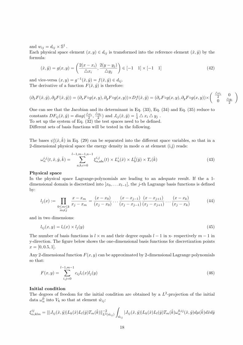
The number of basis functions is l×m and their degree equals l− 1 in x- respectively m− 1 iny-direction. The figure below shows the one-dimensional basis functions for discretization pointsx = [0, 0.5, 1].

Any 2-dimensional function F (x, y) can be approximated by 2-dimensional Lagrange polynomialsso that:

F (x, y) =

l−1,m−1∑i,j=0

cijli(x)lj(y) (46)

Initial conditionThe degrees of freedom for the initial condition are obtained by a L2-projection of the initialdata ω0

α into Vh so that at element wij :

ξijα,klm = ‖|Jij(x, y)|Lk(x)Ll(y)Tm(k)‖−2L2(wij)

∫wij

|Jij(x, y)|Lk(x)Ll(y)Tm(k)ω0,ijα (x, y)dµ(k)dxdy

18

0 0.1 0.2 0.3 0.4 0.5 0.6 0.7 0.8 0.9 1−0.2

0

0.2

0.4

0.6

0.8

1

1.2

L(x)

Lagrange Polynomials

x

Figure 2: Lagrange basis functions up to degree 2

(47)

The calculation can be simplified by using for each element the same integration points xk′ , yl′as the ones used to define the Lagrange polynomials due to the property Li(xi) = 1.Eq. (47) becomes

ξijα,klm = c

∫xy

∫k

Lk(x)Ll(y)Tm(k)ω0,ijα (x, y)dxdydµ(k) =

c

∫k

∫xy

Lk(x)Ll(y)Tm(k)ω0,ijα (x, y)dµ(k)dxdy =

c∑k′l′

∫k

Lk(xk′)Lm(yl′)Tm(k)ω0,ijα (xk′ , yl′)dµ(k) =

d · ω0,ijα (xk, yl) · t(m)

(48)

withd = |Jij |‖Lk(x)Ll(y)Tm(k)|Jij |‖−2

L2(wij) and t(m) =∫kTm(k)dµ(k)

Phase spaceSince by the transformation k = k

|k| the direction of the wave in two dimensions is presenting a

point on the unit circle so that k can be written as k = (cos θ, sin θ).Two ideas arise while trying to find a proper basis decomposition for k. One may immediatelythink of a Fourier series, because its definition includes the sine and cosine functions.Nevertheless unwanted effects such as dissipation and negativity appear. Another idea is torepresent k by a combination of Nurbs basis functions. These have the advantage that theyconserve positivity. In the following the ideas are explained more precisely.

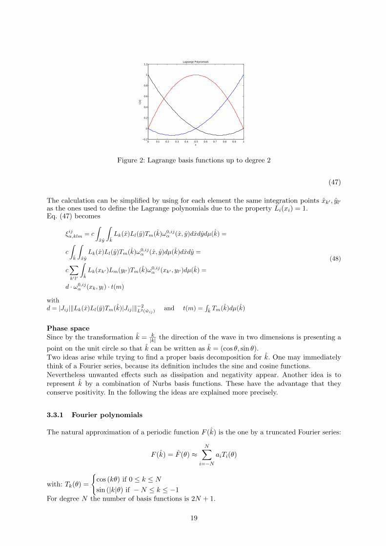
3.3.1 Fourier polynomials

The natural approximation of a periodic function F (k) is the one by a truncated Fourier series:

F (k) = F (θ) ≈N∑

i=−NaiTi(θ)

with: Tk(θ) =

cos (kθ) if 0 ≤ k ≤ Nsin (|k|θ) if −N ≤ k ≤ −1

For degree N the number of basis functions is 2N + 1.

19

Fourier basis functions were used as basis for the spherical space. The figure above shows basisfunctions up to degree 2.

0 1 2 3 4 5 6 7−1

−0.8

−0.6

−0.4

−0.2

0

0.2

0.4

0.6

0.8

1

xT

(x)

Fourier Polynomials

Figure 3: Fourier basis functions of degree up to degree 2

3.3.2 Results

Let the degree of basis functions in x and y direction be equally l − 1 and the degree of basisfunctions for the phase space be n, so that N = 2n+ 1. Then with the definitions:

I = Identity matrix

Cij = diag(cijα )1≤α≤M velocity of ray in mode α at element ij

F (k, k′) =

∫ 1

−1Lk(x)Lk′(x)dx for k, k′ = 0 . . . l − 1

G(l, l′) =

∫ 1

−1Ll(y)Ll′(y)dy for l, l′ = 0 . . .m− 1

U(m,m′) =1

2π

∫ 2π

0Tm(θ)Tm′(θ)dθ for m,m′ = 0 . . . N − 1

V (m,m′) =1

2π

∫ 2π

0Tm(θ)Tm′(θ) cos(θ)dθ for m,m′ = 0 . . . N − 1

W (m,m′) =1

2π

∫ 2π

0Tm(θ)Tm′(θ) sin(θ)dθ for m,m′ = 0 . . . N − 1

P± = (L0(±1)) . . . Ll−1(±1))

V (m,m′)± =1

2

(∫ 2π

0Tm(θ)Tm′(θ) cos(θ)dθ

+−∫ 2π

0Tm(θ)Tm′(θ)| cos(θ)|dθ

)for m,m′ = 0 . . . N − 1

W (m,m′)± =1

2

(∫ 2π

0Tm(θ)Tm′(θ) sin(θ)dθ

+−∫ 2π

0Tm(θ)Tm′(θ)| sin(θ)|dθ

)for m,m′ = 0 . . . N − 1

the matrices in Eq. (32) become:

M ij = JijI ⊗ U ⊗ F ⊗ F (49)

The first term in Eq. (34) writes:

Bij = −2JijCij ⊗ (

1

4xiV ⊗ F ⊗G+

1

4yiW ⊗G⊗ F ) (50)

20

while the second and third terms are summed up into:

2Jij

(1

4xi[Cij ⊗ V + −RRij ]⊗ F ⊗ P+ ⊗ P+ − 1

4xi[Cij ⊗ V − −RLij ]⊗ F ⊗ P− ⊗ P−

+1

4yj[Cij ⊗W+ −RU ij ]⊗ P+ ⊗ P+ ⊗ F − 1

4yj[Cij ⊗W− −RDij ]⊗ P− ⊗ P− ⊗ F

) (51)

The matrix in Eq. (35) describing the neighbor cells is divided into cells that are placed on theleft, the right, above and below the actual cell, so that:

Li+1i−1,j =

2Jij4xi

Ti+1i−1,j ⊗ F ⊗ P± ⊗ P∓ Li,

j+1j−1 =

2Jij4yj

T i,j+1j−1 ⊗ F ⊗ P± +⊗P∓ (52)

The reflection and transmission matrices present the upward, downward, left and right reflectionor transmission.An example of the right reflection matrix is:

RRij = 14π2

∫ π2π2dθ∫ π

2

−π2dθ′ρijαβ(xi− 1

2, θ, θ′)cijβ Tk(θ)Tk′(θ

′) cos θ′

The other matrices are calculated in the same way.

At first sight, the approximation of the phase space by a Fourier series leads to reasonableresult. The wave propagates continuously and the reflection at the boundary is correctly depicted.

with:The picture on the right hand sideshows the reflected wave after two sec-onds. The result seems to be correct intwo dimensions.

t =0.98× T

−L 0 L

L

0

−L

3.3.3 Problems

3.3.3.1 Negativity The phase-space energy densities are non-negative if the initial data isnon-negative. Nevertheless an approximation of the phase space by Fourier polynomials leadsto strong negative values after a short time period. The reason for this are the basis functionscomprised by sine and cosine which are oscillating between −1 and 1.This effect becomes obvious, when y is fixed at a certain point and only the propagation intox-direction is observed as in the figure below.

3.3.3.2 Dispersion To analyze if the wave propagates correctly the dispersive and dissipa-tive behavior must be studied. The theory is brievely explained at the linear advection equationin Rd [1]:

ut + c · ∇u = 0 −∞ < x <∞ (53)

where c is a constant advective field c ∈ Rd.It admits a solution of the form:

u(x, t) = aei(kx−ωt) (54)

21

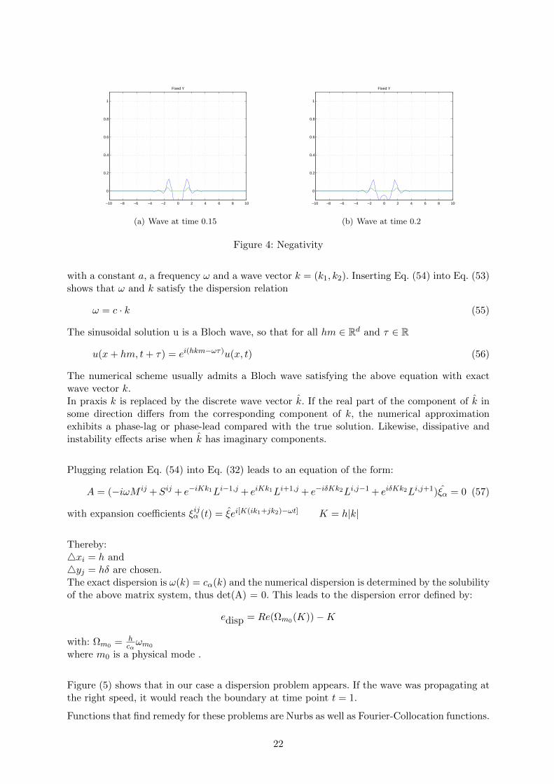
−10 −8 −6 −4 −2 0 2 4 6 8 10

0

0.2

0.4

0.6

0.8

1

Fixed Y

(a) Wave at time 0.15

−10 −8 −6 −4 −2 0 2 4 6 8 10

0

0.2

0.4

0.6

0.8

1

Fixed Y

(b) Wave at time 0.2

Figure 4: Negativity

with a constant a, a frequency ω and a wave vector k = (k1, k2). Inserting Eq. (54) into Eq. (53)shows that ω and k satisfy the dispersion relation

ω = c · k (55)

The sinusoidal solution u is a Bloch wave, so that for all hm ∈ Rd and τ ∈ R

u(x+ hm, t+ τ) = ei(hkm−ωτ)u(x, t) (56)

The numerical scheme usually admits a Bloch wave satisfying the above equation with exactwave vector k.In praxis k is replaced by the discrete wave vector k. If the real part of the component of k insome direction differs from the corresponding component of k, the numerical approximationexhibits a phase-lag or phase-lead compared with the true solution. Likewise, dissipative andinstability effects arise when k has imaginary components.

Plugging relation Eq. (54) into Eq. (32) leads to an equation of the form:

A = (−iωM ij +Sij + e−iKk1Li−1,j + eiKk1Li+1,j + e−iδKk2Li,j−1 + eiδKk2Li,j+1)ξα = 0 (57)

with expansion coefficients ξijα (t) = ξei[K(ik1+jk2)−ωt] K = h|k|

Thereby:4xi = h and4yj = hδ are chosen.The exact dispersion is ω(k) = cα(k) and the numerical dispersion is determined by the solubilityof the above matrix system, thus det(A) = 0. This leads to the dispersion error defined by:

edisp = Re(Ωm0(K))−K

with: Ωm0 = hcαωm0

where m0 is a physical mode .

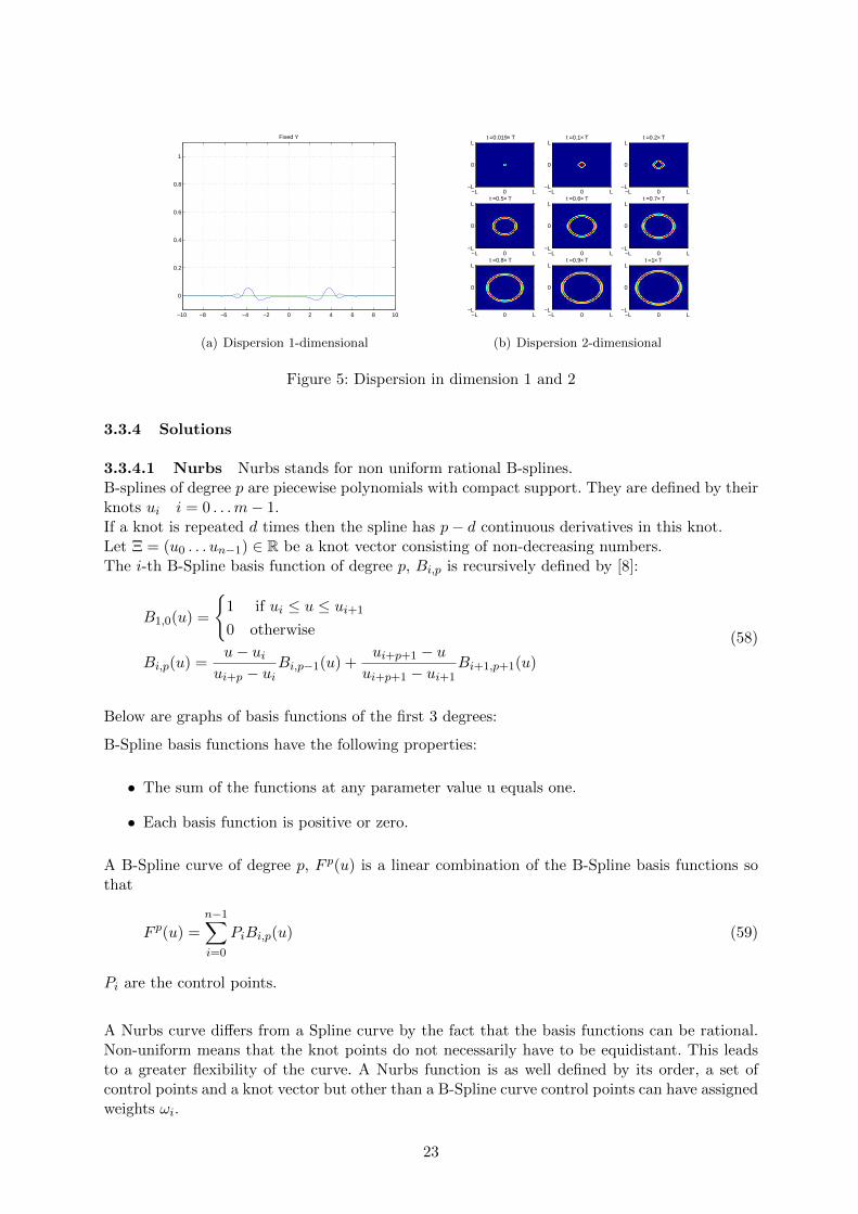
Figure (5) shows that in our case a dispersion problem appears. If the wave was propagating atthe right speed, it would reach the boundary at time point t = 1.

Functions that find remedy for these problems are Nurbs as well as Fourier-Collocation functions.

22

−10 −8 −6 −4 −2 0 2 4 6 8 10

0

0.2

0.4

0.6

0.8

1

Fixed Y

(a) Dispersion 1-dimensional

t =0.019× T

−L 0 L

L

0

−L

t =0.1× T

−L 0 L

L

0

−L

t =0.2× T

−L 0 L

L

0

−L

t =0.5× T

−L 0 L

L

0

−L

t =0.6× T

−L 0 L

L

0

−L

t =0.7× T

−L 0 L

L

0

−L

t =0.8× T

−L 0 L

L

0

−L

t =0.9× T

−L 0 L

L

0

−L

t =1× T

−L 0 L

L

0

−L

(b) Dispersion 2-dimensional

Figure 5: Dispersion in dimension 1 and 2

3.3.4 Solutions

3.3.4.1 Nurbs Nurbs stands for non uniform rational B-splines.B-splines of degree p are piecewise polynomials with compact support. They are defined by theirknots ui i = 0 . . .m− 1.If a knot is repeated d times then the spline has p− d continuous derivatives in this knot.Let Ξ = (u0 . . . un−1) ∈ R be a knot vector consisting of non-decreasing numbers.The i-th B-Spline basis function of degree p, Bi,p is recursively defined by [8]:

B1,0(u) =

1 if ui ≤ u ≤ ui+1

0 otherwise

Bi,p(u) =u− ui

ui+p − uiBi,p−1(u) +

ui+p+1 − uui+p+1 − ui+1

Bi+1,p+1(u)

(58)

Below are graphs of basis functions of the first 3 degrees:

B-Spline basis functions have the following properties:

• The sum of the functions at any parameter value u equals one.

• Each basis function is positive or zero.

A B-Spline curve of degree p, F p(u) is a linear combination of the B-Spline basis functions sothat

F p(u) =

n−1∑i=0

PiBi,p(u) (59)

Pi are the control points.

A Nurbs curve differs from a Spline curve by the fact that the basis functions can be rational.Non-uniform means that the knot points do not necessarily have to be equidistant. This leadsto a greater flexibility of the curve. A Nurbs function is as well defined by its order, a set ofcontrol points and a knot vector but other than a B-Spline curve control points can have assignedweights ωi.

23

0 0.5 1 1.5 2 2.5 3 3.5 4 4.5 50

0.2

0.4

0.6

0.8

1

Nurbs basis functions of degree 0

0 0.5 1 1.5 2 2.5 3 3.5 4 4.5 50

0.1

0.2

0.3

0.4

0.5

0.6

0.7

0.8

0.9

1Nurbs basis functions of degree 1

0 0.5 1 1.5 2 2.5 3 3.5 4 4.5 50

0.1

0.2

0.3

0.4

0.5

0.6

0.7

0.8Nurbs basis functions of degree 2

0 0.5 1 1.5 2 2.5 3 3.5 4 4.5 50

0.1

0.2

0.3

0.4

0.5

0.6

0.7Nurbs basis functions of degree 3

Figure 6: Nurbs basis functions of degree 0 up to 3

A Nurbs basis function of degree p given by:

Ri,p(u) =Bi,p(u)ωi∑n−1i=0 Bi,p(u)ωi

(60)

A Nurbs curve of degree p is defined by:

Np(u) =

n−1∑i=0

PiRi,p(u) (61)

Increasing the value of ωi will pull the curve toward control point Pi.

Note that n, m and p must satisfy m = n+p+1. If all weights are all 1 the Nurbs basis becomesa B-Spline basis. A knot vector is said to be open if its first and last knots are repeated p + 1times. This leads to the fact that the curve is interpolating its control points at the ends.

Approximation of a curveDue to the rational character of Nurbs basis functions, complex objects as circles, ellipses orcylinders can be exactly depicted. For example defining a special knot vector and adequateweights, a circle is generated by a linear combination of Nurbs functions. The knots are thereforedefined by:

knots = [0, 0, 0, 0.25, 0.25, 12 ,

12 ,

34 ,

34 , 1, 1, 1]

weights = [1,√

22 , 1,

√2

2 , 1,√

22 , 1,

√2

2 , 1]

Note that with the above definition of knots, the resulting curve is interpolary at the endpoints and C0 at all other knot points. It seems reasonable to use these basis functions for the

24

0.25 0.3 0.35 0.4 0.45 0.5 0.55 0.6 0.65 0.7 0.750

0.1

0.2

0.3

0.4

0.5

0.6

0.7

0.8

0.9

1Basis functions of degree 2 for a circle

(a) Rational Nurbs basis functions of degree2.

−1 −0.8 −0.6 −0.4 −0.2 0 0.2 0.4 0.6 0.8 1−1

−0.8

−0.6

−0.4

−0.2

0

0.2

0.4

0.6

0.8

1Circle curve

(b) Circle curve that is generated by theright combination of the basis functions.

Figure 7: Circle curve as a combination of Nurbs basis functions

discretization in θ in Eq. (43) since k lies on the unit circle represented by a sum of the productsof 2-dimensional control points and basis functions in u:

(k1(u)k2(u)

)=

(10

)b0,2(u) +

(11

)b1,2(u) +

(01

)b2,2(u) +

(−11

)b3,2(u)+(

−10

)b4,2(u) +

(−1−1

)b5,2(u) +

(0−1

)b6,2(u) +

(1−1

)b7,2(u) +

(10

)b8,2(u)

(62)

The problem with such a definition is, that the functions are discontinuous at the beginningand the end. The point of discontinuity can be observed in the figure at 0 where the circledoes not close. Nevertheless the dispersion problem disappears and the energy density remains

t =0.02× T

−L 0 L

L

0

−L

t =0.1× T

−L 0 L

L

0

−L

t =0.2× T

−L 0 L

L

0

−L

t =0.5× T

−L 0 L

L

0

−L

t =0.6× T

−L 0 L

L

0

−L

t =0.7× T

−L 0 L

L

0

−L

t =0.8× T

−L 0 L

L

0

−L

t =0.9× T

−L 0 L

L

0

−L

t =1× T

−L 0 L

L

0

−L

(a) 2-dimensional spreading energy density for differenttime points t.

0 0.2 0.4 0.6 0.8 1 1.2 1.4 1.6 1.8 20

0.2

0.4

0.6

0.8

1

× T

t

E(t

)

(b) Conservation of the total energy.

Figure 8: Nurbs functions defining a circle

positive.

An immediate observation is the ray effect. This means that the wave carries peaks. These peaksappear at the knots by which the basis functions are defined. One tents to increase the number

25

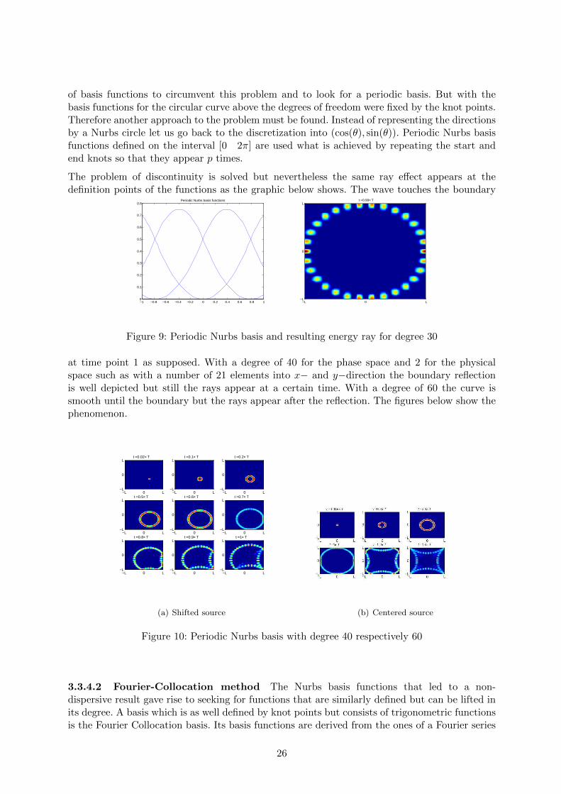
of basis functions to circumvent this problem and to look for a periodic basis. But with thebasis functions for the circular curve above the degrees of freedom were fixed by the knot points.Therefore another approach to the problem must be found. Instead of representing the directionsby a Nurbs circle let us go back to the discretization into (cos(θ), sin(θ)). Periodic Nurbs basisfunctions defined on the interval [0 2π] are used what is achieved by repeating the start andend knots so that they appear p times.

The problem of discontinuity is solved but nevertheless the same ray effect appears at thedefinition points of the functions as the graphic below shows. The wave touches the boundary

−1 −0.8 −0.6 −0.4 −0.2 0 0.2 0.4 0.6 0.8 10

0.1

0.2

0.3

0.4

0.5

0.6

0.7

0.8Periodic Nurbs basis functions t =0.99× T

−L 0 L

L

0

−L

Figure 9: Periodic Nurbs basis and resulting energy ray for degree 30

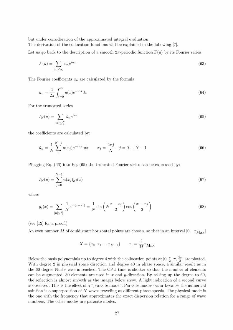
at time point 1 as supposed. With a degree of 40 for the phase space and 2 for the physicalspace such as with a number of 21 elements into x− and y−direction the boundary reflectionis well depicted but still the rays appear at a certain time. With a degree of 60 the curve issmooth until the boundary but the rays appear after the reflection. The figures below show thephenomenon.

t =0.02× T

−L 0 L

L

0

−L

t =0.1× T

−L 0 L

L

0

−L

t =0.2× T

−L 0 L

L

0

−L

t =0.5× T

−L 0 L

L

0

−L

t =0.6× T

−L 0 L

L

0

−L

t =0.7× T

−L 0 L

L

0

−L

t =0.8× T

−L 0 L

L

0

−L

t =0.9× T

−L 0 L

L

0

−L

t =1× T

−L 0 L

L

0

−L

(a) Shifted source (b) Centered source

Figure 10: Periodic Nurbs basis with degree 40 respectively 60

3.3.4.2 Fourier-Collocation method The Nurbs basis functions that led to a non-dispersive result gave rise to seeking for functions that are similarly defined but can be lifted inits degree. A basis which is as well defined by knot points but consists of trigonometric functionsis the Fourier Collocation basis. Its basis functions are derived from the ones of a Fourier series

26

but under consideration of the approximated integral evaluation.The derivation of the collocation functions will be explained in the following [7].

Let us go back to the description of a smooth 2π-periodic function F(u) by its Fourier series

F (u) =∑|n|≤∞

uneinx (63)

The Fourier coefficients un are calculated by the formula:

un =1

2π

∫ 2π

j=0u(x)e−inxdx (64)

For the truncated series

IN (u) =∑|n|≤N

2

uneinx (65)

the coefficients are calculated by:

un =1

N

N−1∑0

u(xj)e−inxjdx xj =

2πj

Nj = 0 . . . N − 1 (66)

Plugging Eq. (66) into Eq. (65) the truncated Fourier series can be expressed by:

IN (u) =N−1∑j=0

u(xj)gj(x) (67)

where

gj(x) =∑|n|≤N

2

1

Nein(x−xj) =

1

Nsin

(Nx− xj

2

)cot

(x− xj

2

)(68)

(see [12] for a proof.)

An even number M of equidistant horizontal points are chosen, so that in an interval [0 xMax]

X = x0, x1 . . . xM−1 xi =i

MxMax

Below the basis polynomials up to degree 4 with the collocation points at [0, π2 , π,3π2 ] are plotted.

With degree 2 in physical space direction and degree 40 in phase space, a similar result as inthe 60 degree Nurbs case is reached. The CPU time is shorter so that the number of elementscan be augmented. 30 elements are used in x and y-direction. By raising up the degree to 60,the reflection is almost smooth as the images below show. A light indication of a second curveis observed. This is the effect of a ”parasite mode”. Parasite modes occur because the numericalsolution is a superposition of N waves traveling at different phase speeds. The physical mode isthe one with the frequency that approximates the exact dispersion relation for a range of wavenumbers. The other modes are parasite modes.

27

0 1 2 3 4 5 6 7−0.2

0

0.2

0.4

0.6

0.8

1

1.2Fourier collocation basis of degree 4

t =0.019× T

−L 0 L

L

0

−L

t =0.1× T

−L 0 L

L

0

−L

t =0.2× T

−L 0 L

L

0

−L

t =0.5× T

−L 0 L

L

0

−L

t =0.6× T

−L 0 L

L

0

−L

t =0.7× T

−L 0 L

L

0

−L

t =0.8× T

−L 0 L

L

0

−L

t =0.9× T

−L 0 L

L

0

−L

t =1× T

−L 0 L

L

0

−L

t =0.019× T

−L 0 L

L

0

−L

t =0.1× T

−L 0 L

L

0

−L

t =0.2× T

−L 0 L

L

0

−L

t =0.5× T

−L 0 L

L

0

−L

t =0.6× T

−L 0 L

L

0

−L

t =0.7× T

−L 0 L

L

0

−L

t =0.8× T

−L 0 L

L

0

−L

t =0.9× T

−L 0 L

L

0

−L

t =1× T

−L 0 L

L

0

−L

Figure 11: Periodic Nurbs basis with degree 40 respectively 60

4 Conclusion

In the paper basis functions for the variational formulation of a radial transport equation wereinvestigated. Whereas the physical space does not cause any problem because of the simple use ofLagrange-functions, the spherical space corresponding to the propagation direction is a difficultissue. So far Lagrange, Fourier, Nurbs and Fourier Collocation basis functions were tested forthe propagation direction. The best result was reached with Fourier Collocation functions withdegree 2 in physical and degree 60 in spherical space and 30 elements in x and y-direction. Thesebasis functions minimize the problems of negativity, dispersion and ray effects. Nevertheless, thematrix of the linear system is huge with number of 1037880 elements, leading to a quite longcalculation time.

5 Outlook

The seeking of optimal basis functions is thus still an ongoing research. Some ideas of other basisfunctions that could be tested are the following;

* Nurbs in 3 dimensions

28

Instead of using different polynomials for the physical and spherical space, Nurbs could bedefined for both of them. This technique is used in isogeometry. In isogemetric analysis,complicated objects are simulated by computer aided design (CAD). This means, thatthey are represented by 2- respectively 3-dimensional Nurbs functions. Once the Nurbs-functions are precised the same functions are used to carry out the analysis i.e. theyare used as basis functions for the FE-method. In our case, this would mean that the2-dimensional plate could be represented by Nurbs functions and the same ones are usedas basis. The problem with Nurbs is that additionally to the knot points, weights mustbe defined which have itself influence of the shape of the curve. For the physical spacethe weights can be set to one since the border is linear. The spherical space is morecomplicated and needs weights other than one. Another difficulty is that the simplificationof the initial condition as indicated in Eq. (47) - Eq. (48) is not possible anymore becauseof the missing property Ni,p(xi) = 1. Instead Eq. (41) needs to be approximated by Nurbs.A surface approximation by Nurbs leads to solving an equational system.

ω0(x, y) =

k−1,l−1∑ij=0

cijNi(x)Nj(y) (69)

so that by choosing at least k × l evaluation points (xi, yj) the system is solvable with:

c = N−1Ω (70)

Ω is the vector formed by ω0(xi, yj).An idea to solve the Nurbs-problem is thus the following:

– Set up a set of 3-dimensional Nurbs-basis functions

– Choose temporary weights for the basis functions

– Modify the weights, so that with c in problem Eq. (70) the representation in Eq. (69)is the best approximation for the initial condition ω0(x, y)

– Use the arising Nurbs basis as basis functions for the physical domain.

– Chose an appropriate Nurbs basis for the spherical domain.

* WaveletsWavelets are mathematical functions that cut up data into different frequency componentswhere each component is studied with a resolution matched to its scale. They have advan-tages over traditional Fourier methods in analyzing physical situations where the signalcontains discontinuities and sharp spikes.Wavelets were developed independently in math-ematics, quantum physics, electrical engineering, and seismic geology. A wavelet basis isdefined by:

ψj,k(x) := 2j/2 ψ(2j x− k) (71)

building a complete orthonormal system in L2(R). ψ can be any wavelet function i.e. theHaar-wavelet.The linear combination of the wavelet basis functions is called wavelet-transformation andis expressed by:

f =∑j,k∈Z

cj,k · ψj,k. (72)

Wavelet have been studied for quite a while and problems are published that made use ofwavelets and the DG-method ([5],[4]). Applying wavelets to our model equation was notpart of the internship but should encourage the reader for further investigations.

29

References

[1] Ainsworth, M. : Dispersive and dissipative behaviour of high order discontinuous Galerkinfinite element methods. In: Journal of Computational Physics 198 (2004), Jul., Nr. 1, S.106–130. – ISSN 0021–9991

[2] Berton, B. : Methode de Galerkin discontinue appliquee a une equation de transport. In:ONERA: Rapport technique de fin d’etude (2010)

[3] Carpenter, M. H.: Fourth-Order 2N-Storage Runge-Kutta Schemes. In: NASA TechnicalMemorandum 109112 (1994), S. 24

[4] Dong Liang, Q. G. ; Gong, S. : Wavelet GalerkinMethods for Aerosol Dynamic Equationsin Atmospheric Environment. In: COMMUNICATIONS IN COMPUTATIONAL PHYSICS6 (2009), S. pp. 109–130

[5] Emmanuil H. Georgoulis, E. H. ; Melenk, J. M.: Wavelets and adaptive grids for thediscontinuous Galerkin method. In: Numerical Algorithms Volume 39 (2005), S. 143–154

[6] Ern, A. ; UPMC-M2R (Hrsg.): Methodes de Galerkin Discontinues et Applications. Par-cours ANEDP, 2007

[7] Hesthaven, J. ; Gottlieb, S. ; Gottlieb, D. : Spectral methods for time-dependentproblems. Cambridge University Press (Cambridge monographs on applied and compu-tational mathematics). http://books.google.com/books?id=dpZg1YEr4GEC. – ISBN9780521792110

[8] Hughes, T. ; Cottrell, J. ; Bazilevs, Y. : Isogeometric analysis: CAD, finite elements,NURBS, exact geometry and mesh refinement. In: Computer Methods in Applied Mechanicsand Engineering 194 (2005), Okt., Nr. 39-41, S. 4135–4195. – ISSN 0045–7825

[9] Kubatko, E. J. ; Westerink, J. J. ; Dawson, C. : Semi discrete discontinu-ous Galerkin methods and stage-exceeding-order, strong-stability-preserving Runge-Kuttatime discretizations. In: Journal of Computational Physics 222 (2007), Nr. 2, S.832 – 848. http://dx.doi.org/DOI: 10.1016/j.jcp.2006.08.005. – DOI DOI:10.1016/j.jcp.2006.08.005. – ISSN 0021–9991

[10] Ryzhik, L. ; Papanicolaou, G. ; Keller, J. B.: Transport equations for elastic and otherwaves in random media. In: Wave Motion 24 (1996), Dez., Nr. 4, S. 327–370. – ISSN0165–2125

[11] Savin, E. : Discontinuous finite element solution of radiative transfer equations for high-frequency power flows in slender structures. In: Rapport technique de l’ONERA (2009),S. 48

[12] Schiemenz, A. R. ; Hesse, M. A. ; Hesthaven, J. S.: Modeling Magma Dynamics with aMixed Fourier Collocation- Discontinuous Galerkin Method. In: Commun. Comput. Phys.10 (2011), S. 433–452

[13] Sigal Gottlieb, E. T. Chi-Wang Shu S. Chi-Wang Shu: Strong-Stability-PreservingHigh-Order Time Discretization Methods. In: SIAM 43 (2001), S. 89–112

30