DELFT UNIVERSITY OF TECHNOLOGY

REPORT 03-01

On a class of preconditioners for solving the Helmholtzequation

Y. A. Erlangga, C. Vuik, C. W. Oosterlee

ISSN 1389-6520

Reports of the Department of Applied Mathematical Analysis

Delft 2003

Copyright 2002 by Department of Applied Mathematical Analysis, Delft, The Netherlands.

No part of the Journal may be reproduced, stored in a retrieval system, or transmitted, inany form or by any means, electronic, mechanical, photocopying, recording, or otherwise,without the prior written permission from Department of Applied Mathematical Analysis,Delft University of Technology, The Netherlands.

On a class of preconditioners for solving the Helmholtz

equation∗

Y. A. Erlangga, C. Vuik, C. W. Oosterlee

January 21, 2003

Abstract

In 1983, Bayliss, Goldstein, and Turkel [2] proposed a preconditioner based onthe Laplace operator for solving the discrete Helmholtz equation efficiently withCGNR. The preconditioner is especially effective for low wavenumber cases wherethe linear system is slightly indefinite. Laird [11] proposed a preconditioner wherean extra term is added to the Laplace operator. This term is similar to that inthe Helmholtz equation but with reversed sign. In this paper, both approaches arefurther generalized to a new class of preconditioners, the so-called ”Shifted Laplace”preconditioners of the form ∆φ−αk2φ with α ∈ C . Numerical experiments for variouswavenumbers indicate the effectiveness of the preconditioner in terms of numbers ofiterations and arithmetic operations. The preconditioner is evaluated in combinationwith GMRES, Bi-CGSTAB, and CGNR.

Keywords: Helmholtz equation, preconditioners, GMRES, Bi-CGSTAB

1 Introduction

In this paper, the time-harmonic wave equation in 2D heterogeneous media is solved nu-merically. The underlying equation governs wave propagations and scattering phenomenaarising in acoustic problems in many areas, e.g., in aeronautics, marine technology, geo-physics, and optical problems. In particular, we look for solutions of the Helmholtz equa-tion discretized by using finite difference discretizations. Since the number of gridpointsper wavelength should be sufficiently fine to result in acceptable solutions, for very highwavenumbers the discrete problem becomes extremely large, prohibiting the use of direct

∗This research is financially supported by the Dutch Ministry of Economic Affairs under the projectBTS01044 ”Rigorous modelling of 3D wave propagation in inhomogeneous media for geophysical andoptical problems”

1

methods. Iterative methods are the interesting alternative. However, Krylov subspacemethods are not competitive without a good preconditioner. In this paper, we consider aclass of preconditioners to improve the convergence of the Krylov subspace methods.

Various authors contributed to the development of powerful preconditioners for Helm-holtz problems. The work in [2] and the follow-up investigation in [9] can be considered asthe start for the class of preconditioners we are interested in. A generalization has beenrecently proposed in [11]. In [2, 9, 11], the preconditioners are constructed based on theLaplace operator. In [11], this operator is perturbed by a real-valued linear term. Thissurprisingly straightforward idea leads to very satisfactorily convergence. Furthermore,the preconditioning matrix allows the use of SSOR, ILU, or multigrid to approximate theinversion within an iteration.

In this paper, we will generalize the approach in [2, 9, 11]. We give theoritical andnumerical evidence that introducing a complex perturbation to the Laplace operator canresult in a better preconditioner than using a real-valued perturbation. We call the resultingclass of preconditioners ”Shifted Laplace” preconditioners. This class of preconditioners issimple to construct and is easy to extend to inhomogeneous media.

There are various other types of preconditioners for general indefinite linear systems,e.g. [6, 8, 12, 14]. In particular for Helmholtz problems, [8] proposed a class of precon-ditioners (so called AILU) based on a parabolic factorization of the Helmholtz operator.In [12] another approach is pursued by perturbing the real part of the matrix to make itless indefinite. An interesting alternative is also described in [14], where a preconditionerbased on the separation of variables is proposed. This preconditioner effectively acceleratesthe convergence for high wavenumbers.

This paper is organized as follows. In Section 2 we describe the mathematical modeland the discretization used to solve wave propagation problems. Iterative methods usedto solve the resulting linear system and the preconditioner will be discussed in Sections 3and 4 respectively. In Section 5, we present the Shifted Laplace preconditioners and showtheoretically the convergence of this type of preconditioner. Numerical results are thenpresented in Section 6.

2 Mathematical model

We solve wave propagations in a two dimensional medium with inhomogeneous propertiesin a unit (scaled) domain governed by the Helmholtz equation

∆φ + k2(x, y)φ = f, Ω = [0, 1]2, (1)

where ∆ ≡ ∂2/∂x2 + ∂2/∂y2, the Laplace operator, and k(x, y) ∈ R is the wavenumber,which may depend on the spatial position in the domain. We consider a so-called ”openproblem”, i.e., outgoing waves penetrate at least at one boundary without (spurious) reflec-tions. To satisfy this condition, a radiation-type condition is imposed. Several formulationshave been developed to model the non-reflecting condition at the boundary [1, 3, 4]. In

2

this paper, the first order Sommerfeld condition is chosen of the form

∂φ

∂n− ikφ = 0, on a part of Γ = ∂Ω (2)

with n an outward direction normal to the boundary. Eventhough (2) may not be suffi-ciently accurate for inclined outgoing waves [4], it is state-of-the-art in industrial codes,easy to implement in our discretization, and requires only a few gridpoints. We anticipatefor possible reflections by considering a sufficiently large domain enabling any wave reflec-tions to be immediately damped out and therefore be localized in the neighborhood of theboundaries.

To find numerical solutions of (1), the equation is discretized using the second-orderdifference scheme, in x-direction:

∂2φ

∂x2=

1

∆x2(φi−1 − 2φi + φi+1) + O(∆x2), (3)

and similar in y-direction. The first order derivative in (2) is discretized with the first orderforward scheme

∂φ

∂n=

1

∆n(φi+1 − φi) . (4)

Substituting (3) and (4) into (1) and (2), one obtains a linear system

Ap = b, A ∈ CN×N , (5)

where A is a large, sparse symmetric matrix, and N is the number of gridpoints. Matrix Ais complex-valued and indefinite for large values of k. Throughout this paper, we say ”Ais indefinite” if A has eigenvalues with a positive real part and eigenvalues with negativereal part [6].

3 Krylov subspace method

For a large, but sparse matrix, Krylov subspace methods are very popular. The methodsare developed based on a construction of iterants in the subspace

Kj(A, r0) = spanr0, Ar0, A2r0, · · · , Aj−1r0, (6)

where Kj(A, r0) is the j-th Krylov subspace associated with A and r0 (see, e.g., [16]).The basic algorithm within this class is the Conjugate Gradient method (CG) which

has the nice properties that it uses only three vectors in memory and minimizes the errorin the A-norm. However, the algorithm mainly performs well if the matrix A is symmetric,and positive definite. In cases where one of these two properties is violated, CG may breakdown. For indefinite linear systems, CG can be applied to the normal equations since theresulting linear system becomes (positive) definite. Upon application of CG to the normalequations, CGNR [16] results. Using CGNR, the iterations are guaranteed to converge.

3

The drawback is that the condition number of the normal equations equals the square ofthe condition number of A, slowing down the convergence drastically.

Some algorithms with short recurrences but without the minimizing property are con-structed based on the bi-Lanczos algorithm [16]. Within this class, BiCG [5] exists andits modifications: CGS [19] and Bi-CGSTAB [20]. In BiCG, the Krylov subspace is con-structed from the orthogonalization of two residual vectors based on actual matrix A andits transpose AT . Accordingly, one extra matrix/vector multiplication and one transposeoperation are needed. In CGS, the extra transpose operation can be avoided. One can ac-celerate the convergence by squaring the polynomial. Whenever the convergence is smooth,CGS converges twice as fast as BiCG. However, if the BiCG iteration diverges, CGS alsodiverges twice as fast as BiCG. To stabilize CGS, rather than taking the square of thepolynomial, another polynomial can be chosen and multiplied with the polynomial of A.This results in Bi-CGSTAB. In many cases, Bi-CGSTAB exhibits a smooth convergencebehavior and often converges faster than CGS. Also within this class are QMR [7] andCOCG [21].

MINRES [13] can also be used to solve indefinite symmetric linear systems, as wellas its generalization to the nonsymmetric case, GMRES [17, 16]. Both algorithms havethe minimization property but GMRES uses long reccurences. GMRES has the advantagethat theoretically the algorithm does not break down unless convergence has been reached.The main problem in GMRES is that the amount of storage increases as the iterationnumber increases. Therefore, the application of GMRES may be limited by the computerstorage. To remedy this problem, a restarted version, GMRES(m), can be utilized [17].Since restarting removes the previous convergence history, GMRES(m) is not guaranteedto converge. There is no specific rule to determine the restart parameter m. In casescharacterized by superlinear convergence, m should often be chosen very large which makesrestarting much less attractive. Another way to remedy the storage problem in GMRESis by including a so-called ”inner iteration” as in GMRESR [22] and FGMRES [15].

Since the convergence theory of GMRES is well established, in our numerical experi-ments mainly full GMRES is used. Of course, experiments then become very restrictive(in this paper, upto k = 30) and for large problems, restarts become necessary. We alsocompute solutions using Bi-CGSTAB and compare the convergence results with GMRES.For completeness, since the underlying theory on the preconditioners is developed basedon the normal equations [11], we also include the convergence results using CGNR in thelast experiment.

4 Preconditioner

To improve the convergence of iterative methods, a preconditioner should be incorporated.By left preconditioning, one solves a linear system premultiplied by a preconditioning

matrix M−1,M−1Ap = M−1b. (7)

4

Often, right preconditioning is used, i.e.,

AM−1p = b, (8)

where p = Mp. Both preconditionings show typically a very similar convergence be-havior. However, for left preconditioning GMRES computes the residuals based on thepreconditioned system. In contrast, for right preconditioning GMRES computes the ac-tual residuals. This difference may affect the stopping criterion to be used (see discussionsin [16]).

The best choice for M−1 is the inverse of A, which is impractical. If A is SPD, onecan approximate A−1 by one iteration of SSOR or multigrid. However, most practicalwave problems result in an indefinite linear system, for which SSOR or multigrid are notguaranteed to converge (and do not converge).

In general, one can distinguish two approaches for constructing preconditioners: matrix-based and operator-based. Within the first class lie, e.g., incomplete LU (ILU) factoriza-tions. Several ILU techniques have been developed with different choices of the toleratedfill-in in the sparsity pattern of A, e.g., zero fill-in ILU, or ILU with drop tolerance. Anotherdifferent approach but falling into this category is the approximate inverse (see, e.g., [16]).An example of an operator-based preconditioner is analytic ILU (AILU) [8], which is basedon the continuous Helmholtz operator.

In the next sections, we will briefly discuss some preconditioners for Helmholtz prob-lems.

4.1 ILU preconditioner

An ILU preconditioner can be constructed by performing Gauss elimination and droppingsome elements based on certain criteria. One can, e.g., drop all elements except for thosein the same diagonals as the original matrix. This leads to ILU(0). ILU(p) allows fill-inin p additional diagonals. One can also drop elements which are smaller than a specifiedvalue, giving ILU(tol). In applications involving M -matrices, this class of preconditioners issufficiently effective. However, preconditioners from this class are not effective for generalindefinite problems. Reference [8] shows some results in which ILU-type preconditionersare used to solve the Helmholtz equation using QMR. For high wavenumbers k, ILU(0)converges slowly, while ILU(tol) encounters storage problems (and also slow convergence).For sufficiently high wavenumbers k, the cost to construct the ILU(tol) factors may becomevery high.

Instead of constructing the ILU factors from A, the Helmholtz operator Lh = ∆ + k2

can be used to set up ILU-like factors in so-called analytic ILU (AILU) [8]. Starting withthe Fourier transform of the analytic operator in one direction, one constructs parabolicfactors of the Helmholtz operator consisting of a first order derivative in one directionand a non-local operator. To remove the non-local operator, a localized approximation isproposed, involving optimization parameters. Finding a good approximation for inhomo-geneous problems is the major difficulty in this type of preconditioner. This is because the

5

method is sensitive with respect to small changes in these parameters. The optimizationparameters depend on k(x, y).

4.2 Shifted Laplace preconditioner

Another approach is found in not looking for an approximate inverse of the discrete in-definite operator A, but merely looking for a form of M , for which M −1A has satisfactoryproperties for Krylov subspace acceleration. A first effort to construct a preconditionerin such a way is in [2]. An easy-to-construct M = ∆ preconditioner is incorporated forCGNR. One SSOR iteration is used whenever operations involving M −1 are required. Thesubsequent work on this preconditioner with multigrid was done in [9].

Instead of the Laplace operator as the preconditioner, [11] investigates possible improve-ments if an extra term −k2 is added to the Laplace operator. So, the Helmholtz equationwith reversed sign is proposed as the preconditioner M . This preconditioner is then usedin CGNR. One multigrid iteration is employed whenever M −1 must be computed. Insteadof the normal equations, our findings suggest that GMRES can solve the preconditionedlinear system efficiently in less arithmetic operations, despite of a storage problem for highk. However, the latter problem can be overcome, e.g., by applying GMRES(m) or GM-RESR. Bi-CGSTAB, which is considered a good alternative except for more matrix/vectormultiplications, does not perform satisfactorily [11]. (See also results in Section 6.)

In the next section, we concentrate on this type of preconditioners and present a gen-eralization.

5 Spectral properties of Shifted Laplace precondition-

ers

In this section we provide some analysis to understand the performance of the ShiftedLaplace preconditioners. The analysis is based on eigenvalue properties of the precondi-tioned system. It is often that the eigenvalue distribution can help in understanding thebehavior of CG-like iterations. Since the spectra of M −1A and AM−1 are identical, weconcentrate on left preconditioning.

5.1 Real Shifted-Laplace preconditioner

The preconditioners in [2, 11] can be motivated as follows. Consider the continuous 1DHelmholtz equation, subject to discretization. For simplicity, suppose that both boundaryconditions are either Dirichlet or Neumann conditions.

We first consider the eigenvalues for the 1D Helmholtz operator without any precondi-tioning. Eigenvalues of this standard problem, denoted by λs, are found to be

λsn = k2

n − k2, kn = nπ, n ∈ N\0. (9)

6

In (9), kn is the natural frequency of the system. (We use n to indicate the eigenmodes).If one considers the modulus of the eigenvalues (which in this case is simply their absolutevalue), it is easily seen that |λ| becomes unbounded if either n or k are large. If the l 2-condition number κ = |λmax/λmin| is used to evaluate the quality of eigenvalue clustering,one concludes that for any sufficiently small λmin the condition number is extremely large.

Now, suppose an operator of the form

d2

dx2− αk2, α ≥ 0 ∈ R (10)

is used as a preconditioner, constructed with the same discretization stencil and boundaryconditions. The following generalized eigenvalue problem is obtained, i.e.,

(

d2

dx2+ k2

)

φv = λ

(

d2

dx2− αk2

)

φv, x ∈ [0, 1] ⊆ R. (11)

For (11), we find the eigenvalues to be

λn =k2

n − k2

k2n + αk2

=1 − (k/kn)

2

1 + α(k/kn)2, n ∈ N\0. (12)

For n → ∞, λn → 1, i.e. the eigenvalues are bounded above by one. Examining the loweigenmodes, for kn → 0, we obtain λ → −1/α. This eigenvalue remains below one unlessα ≤ 1. The maximum eigenvalue can thus be written as

|λmax| = max

(

| 1α|, 1)

, α ≥ 0 ∈ R. (13)

To estimate the minimum eigenvalue, one can use a simple but rough analysis as follows.It is assumed that the minimum eigenvalue is very close (but not equal) to zero. Thisassumption indicates a condition kj ≈ k as obtained from (12). To be more precise, letkj = k + ε, where ε is any small number. If this relation is substituted into (12), and ifhigher order terms are neglected, and εk k2 is assumed, then we find

λmin =2

1 + α

( ε

k

)

. (14)

From (14), the minimum eigenvalue can be very close to zero as α goes to infinity. Thecondition number of the preconditioned Helmholtz operator now reads

κ =

1

2(1 + α)k/ε if α ≥ 1,1

2α(1 + α)k/ε if 0 ≤ α ≤ 1.

(15)

If α ≥ 1, κ is a monotonically increasing function with respect to α. The best choice isα = 1, which gives minimal κ. If 0 ≤ α ≤ 1, κ is a monotonically decreasing function withrespect to α. κ is minimal in this range if α = 1. In the limit sense we find that

limα↓1

κ = limα↑1

κ = k/ε, (16)

which is the minimum value of κ for α ≥ 0 ∈ R.

7

5.2 Generalization to complex α

The analysis on 1D Shifted Laplace preconditioners for α ∈ R gives α = 1 as the optimumcase. The nice property of the real Shifted Laplace operator, at least in 1D, is that theeigenvalues have an upper bound. However, this property does not guarantee that theeigenvalues are favourably distributed. There is still the possibility that one or someeigenvalues (which are extremely small) can be very close to zero. We can improve thepreconditioner by preserving the upper boundedness and at the same time shifting theminimum eigenvalue as far as possible from zero. In this section, we generalize α to becomplex-valued.

Consider the minimum eigenvalue λmin obtained from the 1D problem (14). We haveshifted this eigenvalue away from zero by adding some real values to λ. In general, thisaddition will shift all eigenvalues, which is undesirable. An alternative is multiplying theeigenvalues by a factor. From (12) the relation between eigenvalues for α = 0 and α = 1reads

(λα=1)n =1

1 + (k/kn)2(λα=0)n . (17)

Equation (17) indicates that λα=0 is scaled by a factor 1 + (k/kn)2. Now we shift theminimum eigenvalue as far as possible away from zero. Using (14), we obtain the followingrelation:

(λα=1)min=

1

2(λα=0)min

. (18)

We generalize the same process to the complex plane: shifting the eigenvalues alongthe complex axis away from zero. We introduce a complex coefficient of the form α + iβ,and consider a more general complex-valued Shifted Laplace operator

d2

dx2− (α + iβ)k2, α ≥ 0 ∈ R, β ∈ R . (19)

Eigenvalues of the premultiplied equation, denoted by λ c, are

λc =k2

n − k2

k2n + (α + iβ)k2

⇒ |λc|2 =(k2

n − k2)2

(k2n + αk2)2 + β2k2

. (20)

Evaluating λmax and λmin as in (13) and (14) one finds

|λcmax|2 = max

(

1

α2 + β2, 1

)

, |λcmin|2 =

4

(1 + α)2 + β2

( ε

k

)2

. (21)

These results give the following condition numbers

κ2 =

1

4

(

1 + 1+2αα2+β2

)

(k/ε)2, α2 + β2 ≤ 1,

1

4((1 + α)2 + β2) (k/ε)2, α2 + β2 ≥ 1.

(22)

Since α2 + β2 is non-negative, for any given α taking the circle α2 + β2 = 1 in the firstexpression in (22) provides the smallest κ2. Likewise, for any given α, κ2 is minimal for

8

−10 0 10

−1

−0.5

0

0.5

1

alpha = 0, beta = 0

Real

Imag

−1 0 1

−1

−0.5

0

0.5

1

alpha = 1, beta = 0

Real−1 0 1

−1

−0.5

0

0.5

1

alpha = 0, beta = 1

Real

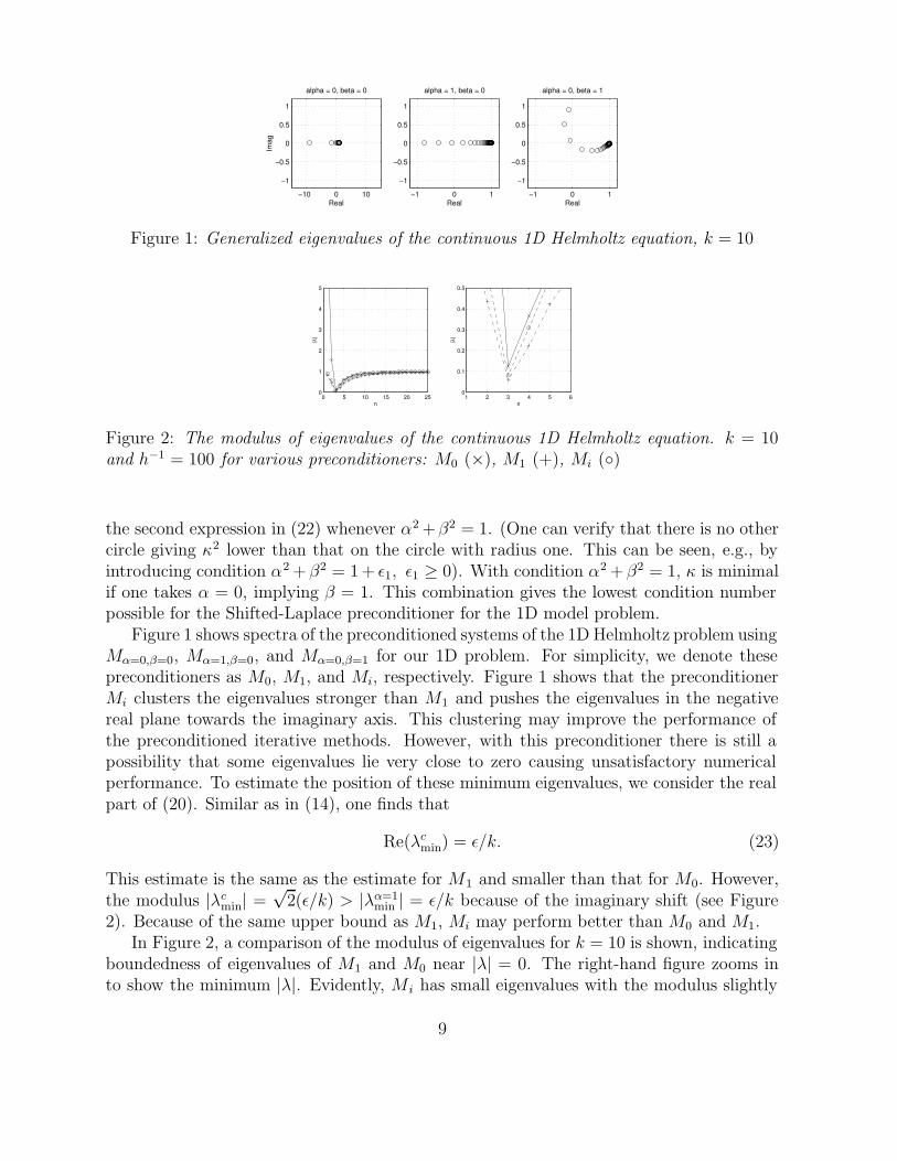
Figure 1: Generalized eigenvalues of the continuous 1D Helmholtz equation, k = 10

0 5 10 15 20 250

1

2

3

4

5

n

|λ|

1 2 3 4 5 60

0.1

0.2

0.3

0.4

0.5

n

|λ|

Figure 2: The modulus of eigenvalues of the continuous 1D Helmholtz equation. k = 10and h−1 = 100 for various preconditioners: M0 (×), M1 (+), Mi ()

the second expression in (22) whenever α2 +β2 = 1. (One can verify that there is no othercircle giving κ2 lower than that on the circle with radius one. This can be seen, e.g., byintroducing condition α2 + β2 = 1 + ε1, ε1 ≥ 0). With condition α2 + β2 = 1, κ is minimalif one takes α = 0, implying β = 1. This combination gives the lowest condition numberpossible for the Shifted-Laplace preconditioner for the 1D model problem.

Figure 1 shows spectra of the preconditioned systems of the 1D Helmholtz problem usingMα=0,β=0, Mα=1,β=0, and Mα=0,β=1 for our 1D problem. For simplicity, we denote thesepreconditioners as M0, M1, and Mi, respectively. Figure 1 shows that the preconditionerMi clusters the eigenvalues stronger than M1 and pushes the eigenvalues in the negativereal plane towards the imaginary axis. This clustering may improve the performance ofthe preconditioned iterative methods. However, with this preconditioner there is still apossibility that some eigenvalues lie very close to zero causing unsatisfactory numericalperformance. To estimate the position of these minimum eigenvalues, we consider the realpart of (20). Similar as in (14), one finds that

Re(λcmin) = ε/k. (23)

This estimate is the same as the estimate for M1 and smaller than that for M0. However,the modulus |λc

min| =√

2(ε/k) > |λα=1min | = ε/k because of the imaginary shift (see Figure

2). Because of the same upper bound as M1, Mi may perform better than M0 and M1.In Figure 2, a comparison of the modulus of eigenvalues for k = 10 is shown, indicating

boundedness of eigenvalues of M1 and M0 near |λ| = 0. The right-hand figure zooms into show the minimum |λ|. Evidently, M i has small eigenvalues with the modulus slightly

9

larger than M1, but smaller than M0.

5.3 Spectrum of the discrete Helmholtz equation

We extend the analysis to the discrete formulation of (1). Suppose that the Helmholtzequation is discretized, we arrive at the linear system Ap = b.

Matrix A can be splitted into two parts: the Laplace component B and the additionaldiagonal term k2I so that A = B + k2I and therefore

(

B + k2I)

p = b. (24)

In this analysis, we use only Dirichlet or Neumann conditions at the boundaries in orderto keep the matrix A real-valued. We precondition (24) using M = B − (α + iβ)k 2I,constructed with the same boundary conditions as for A. This gives

(

B − (α + iβ)k2I)−1 (

B + k2I)

p =(

B − (α + iβ)k2I)−1

b. (25)

The generalized eigenvalue problem of (25) is accordingly

(

B + k2I)

pv = λv

(

B − (α + iβ)k2I)

pv. (26)

Both systems (25) and (26) are indefinite if k2 is larger than the smallest eigenvalueof B. In such a case, the convergence is difficult to estimate. Therefore, the subsequentanalysis will be based on the normal equations formulation of the preconditioned matrixsystem (as in [11]).

Denote the eigenvalues of B as 0 < µ1 ≤ µ2 ≤ · · · ≤ µn. We find for the eigenvalues ofthe four following cases:

λ (A∗A) =(

µi − k2)2

, (27)

λ((

M−10 A

)∗ (

M−10 A

))

=

(

µi − k2

µi

)2

=

(

1 − k2

µi

)2

, (28)

λ((

M−11 A

)∗ (

M−11 A

))

=

(

µi − k2

µi + k2

)2

=

(

1 − 2k2

µi + k2

)2

, (29)

λ((

M−1

i A)∗ (

M−1

i A))

=

(

µi − k2

µi + ik2

)(

µi − k2

µi + ik2

)

= 1 − 2µik2

µ2i + k4

. (30)

10

For all cases, we find for the minimal and maximal eigenvalue, if k ∈ R, 0 < k2 < µ1,

λ ((A∗A))min

=(

µ1 − k2)2

,

λ ((A∗A))max

=(

µn − k2)2

, (31)

λ((

M−10 A

)∗ (

M−10 A

))

min=

(

1 − k2

µ1

)2

,

λ((

M−10 A

)∗ (

M−10 A

))

max=

(

1 − k2

µn

)2

, (32)

λ((

M−11 A

)∗ (

M−11 A

))

min=

(

1 − 2k2

µ1 + k2

)2

,

λ((

M−11 A

)∗ (

M−11 A

))

min=

(

1 − 2k2

µn + k2

)2

, (33)

λ((

M−1i A

)∗ (

M−1i A

))

min= 1 − 2µ1k

2

µ21 + k4

,

λ((

M−1i A

)∗ (

M−1i A

))

max= 1 − 2µnk2

µ2n + k4

. (34)

Since k2/µ1 < 1, one easily sees that

λ(

(M−10 A)∗(M−1

0 A))

min> λ

(

(M−11 A)∗(M−1

1 A))

min.

As n → ∞, one finds also that

limµn→∞

λ(

(M−10 A)∗(M−1

0 A))

max= lim

µn→∞λ(

(M−11 A)∗(M−1

1 A))

max= 1.

With respect to the l2-condition number, it becomes evident that for frequencies lowerthan

õ1, M0 may be better than M1. For Mi, one can compute that

λ((

M−1i A

)∗ (

M−1i A

))

min/λ((

M−10 A

)∗ (

M−10 A

))

min=

(µ1 + k2)2

µ21 + k4

> 1,

limµn→∞

λ((

M−1i A

)∗ (

M−1i A

))

max= 1.

Furthermore, λ ((MiA)∗(MiA))min

≤ λ ((M0A)∗(M0A))min

. So, for frequencies lower thanõ1, M0 may perform better than any other choice. However, the main focus is on high

wavenumbers which are of practical interests.If now µ1 < k2 < µn, we encounter an indefinite problem. However, for the standard

A∗A, one finds

λ (A∗A)min

=(

µm1− k2

)2, where |µm1

− k2| ≤ |µi − k2|, ∀i,

λ (A∗A)max

=(

µn − k2)2

,(35)

11

which is always positive definite. In this case, the eigenvalues are unbounded either forlarge µn or large k. For the preconditioned system (M−1

0 A)∗(M−10 A) one finds

λ(

(M−10 A)∗(M−1

0 A))

min=

(

µm2− k2

µm2

)2

,

where |µm2− k2

µm2

| ≤ |µi − k2

µi

|, ∀i,

λ(

(M−10 A)∗(M−1

0 A))

max= max

(

(

µn − k2

µn

)2

,

(

µ1 − k2

µ1

)2)

. (36)

In this case, there will be a possible boundedness for large µn, i.e., for µn → ∞, λn = 1 aslong as k is finite ( because limk→∞((µi − k2)/(µi))

2 = ∞). Furthermore, limµ1→0((µ1 −k2)/(µ1))

2 = ∞. Therefore, λmax can become extremely large, which makes M0 less favor-able for preconditioning.

For the preconditioned system (M−11 A)∗(M−1

1 A), one finds that

λ(

(M−11 A)∗(M−1

1 A))

min=

(

µm3− k2

µm3+ k2

)2

,

where |µm3− k2

µm3+ k2

| ≤ | µi − k2

µi + µm3

|, ∀i,

λ(

(M−11 A)∗(M−1

1 A))

max= max

(

(

µn − k2

µn + k2

)2

,

(

µ1 − k2

µ1 + k2

)2)

. (37)

From (37), it is found that

limµn→∞

(

µn − k2

µn + k2

)2

= limµ1→0

(

µ1 − k2

µ1 + k2

)2

= limk→∞

(

µi − k2

µi + k2

)2

= 1. (38)

For all possible extreme cases, the preconditioned system M −11 A is always bounded above

by one, i.e. the eigenvalues are always clustered. We can conclude that in the indefinitecase M1 may be better than M0.

Finally, we are looking at the complex shifted preconditioned system with M i. Onefinds that

λ(

(M−1i A)∗(M−1

i A))

min=

(µm4− k2)2

µ2m4

+ k4,

where |(µm4− k2)2

µ2m4

+ k4| ≤ |(µi − k2)2

µ2i + k4

|, ∀i,

λ(

(M−1i A)∗(M−1

i A))

max= max

(

1 − 2µ1k2

µ21 + k4

, 1 − 2µnk2

µ2n + k4

)

. (39)

12

The following results follow:

limµn→∞

λ(

(M−1i A)∗(M−1

i A))

max= lim

µ1→0λ(

(M−1i A)∗(M−1

i A))

max=

= limk→∞

λ(

(M−1i A)∗(M−1

i A))

max= 1. (40)

Hence, the eigenvalues of (M−1i A)∗(M−1

i A) are always bounded above by one.To determine the lower bound, we assume that λmin ≈ 0 implying µm = k2 + ε, ε > 0.

After substituting this relation to (39), one finds that

λ(

(M−1i A)∗(M−1

i A))

min=

1

2

ε2

k4. (41)

Comparing to M1 preconditioning (where λ(

(M−11 A)∗(M−1

1 A))

min= 1

4ε2/k4), it follows

that λ(

(M−1i A)∗(M−1

i A))

min= 2λ

(

(M−11 A)∗(M−1

1 A))

min. With respect to the l2−condit-

ion number, one finds that

κ(

(M−1i A)∗(M−1

i A))

= 2

(

k4

ε2

)

< κ(

(M−11 A)∗(M−1

1 A))

= 4

(

k4

ε2

)

.

We conclude that Mi may be a better preconditioner than M1. Mi also may be betterthan M0, which has possibly unbounded eigenvalues (and therefore a very large conditionnumber) if µ is very small and µ k.

6 Numerical results

We provide some numerical results for solving equation (1), and present three cases as themodel problems: (i) a 2-D closed-off problem with Dirichlet conditions at all boundaries,(ii) a 2-D open problem in a homogeneous medium with Sommerfeld conditions on a partof the boundary, and (iii) a 2-D open problem in an inhomogeneous medium.

For all cases, we solve the resulting linear system with full GMRES and compare threepreconditioners M0, M1, and Mi. We set the maximum number of GMRES iterationsto 150. Beyond this value, we restart GMRES. As k increases considerably, storing 150vectors becomes too expensive, requiring a smaller restart parameter. This is the maindrawback of using GMRES. Therefore, for the third problem the GMRES convergence iscompared to that of CGNR and Bi-CGSTAB. The iteration is terminated at the k-th step if‖rk‖2/‖b‖2 < 10−6. The step involving M−1 is accomplished by using Gauss elimination.In practice this process is very costly. Of course, since M is symmetric and both thereal and imaginary parts are positive definite, the LDLT factorization can always be done(without requiring pivoting) and is unique [10]. We can also approximate M −1 using SSORor multigrid. We do not implement these cheaper processes. The direct computation ofM−1 can be used as a reference for approximations of M−1.

13

−1 0 1−1

−0.5

0

0.5

1

Real

Imag

−1 0 1−1

−0.5

0

0.5

1

Real−1 0 1

−1

−0.5

0

0.5

1

Real

Figure 3: Some extreme eigenvalues of the preconditioned systems of Problem 1 with k = 5and gridsize h−1 = 20

6.1 Closed-off problem

We consider a problem in a rectangular homogeneous medium governed by

(

∆ + k2)

φ = (k2 − 5π2) sin(πx) sin(2πy), x = [0, 1], y = [0, 1],

φ = 0, at the boundaries.(42)

The exact solution of (42) is φ = sin(πx) sin(2πy). Different grid resolutions are usedto solve the problem with various wavenumbers k = 2, 5, 10, 15, 20. k = 2 resembles thedefinite problem. In Figure 3, spectra of the preconditioned system for k = 5, a ”slightly”indefinite problem, are shown. All spectra are bounded above by one.

Table 1 shows the computational performance in terms of number of iterations andnumber of arithmetic operations to reach the specified convergence. For low frequencies,all preconditioners show a very satisfactorily comparable performance. It appears that M 0

becomes less effective for increasing values of k, where the number of iterations increasessomewhat faster than for M1 or Mi. This behavior agrees with the theory.

In Table 2, the numerical performance is shown for the preconditioners for differentgrid resolutions. The preconditioners are sensitive with respect to the grid sizes. For allcases, Mi outperforms the other preconditioners.

6.2 2-D open homogeneous problem

The second problem represents an open problem allowing waves to penetrate the bound-aries. We first look at a homogeneous medium in which waves created at the upper surfacepropagate. We consider

∆φ + k2φ = f, Ω = [0, 1]2,

f = δ(x − 1/2)δ(y), x = [0, 1], y = 0,

φ = 0, y = 0,

∂φ

∂n− ikφ = 0, x = 0, 1, y = 1,

(43)

with k constant in Ω. The performance of GMRES with M0, M1, and Mi as the precon-ditioners is compared.

14

Table 1: Computational performance of GMRES for 2-D closed-off problem. The precon-ditioner is the Shifted Laplace operator. 30 gridpoints per wavelength are used. The flopsare measured in millions

M0 M1 Mi

k Iter flops Iter flops Iter flops

2 4 0.008 4 0.008 4 0.010

5 6 0.093 7 0.106 6 0.012

10 10 0.628 11 0.684 10 0.752

15 16 2.223 18 2.481 16 2.623

20 30 7.256 25 6.091 23 5.627

30 38 20.753 34 18.633 31 17.046

40 57 55.133 46 44.677 37 36.157

Table 2: Number of GMRES iterations to solve Problem 1 with various grid resolutions.The preconditioner is the Shifted Laplace operator

M0 M1 Mi

h−1 h−1 h−1

k 50 100 150 50 100 150 50 100 150

5 5 5 5 6 6 6 6 6 5

10 10 10 10 11 11 11 10 10 10

15 17 14 14 19 15 15 17 14 14

20 33 30 21 37 25 21 31 23 19

30 79 55 38 86 57 34 72 52 31

15

−1 0 1−0.5

0

0.5

1

Real

Imag

−1 0 1−0.5

0

0.5

1

Real

Imag

−1 0 1−0.5

0

0.5

1

Real

Imag

Figure 4: Spectra of the linear systems from Problem 2 preconditioned with M0 (left), M1

(middle), and Mi (right). The radiation condition is replaced by a Dirichlet condition fork = 5 with h−1 = 10 (∼ 10 gridpoints per wavelength)

The Sommerfeld condition is set in the problem to avoid non-physical reflections. How-ever, this may not be important for the preconditioning operator. We prefer to replaceSommerfeld’s condition in the preconditioner by simpler a boundary condition. For thispurpose, we use the Neumann or Dirichlet conditions in M . To see the effect of imposingdifferent types of boundary conditions on the convergence performance, we analyze thespectra of the preconditioned linear systems.

Figure 4–6 show spectra of the preconditioned linear systems of Problem 2. The Jacobi-Davidson algorithm [18] is used to compute some extreme eigenvalues. Imposing eitherDirichlet or Neumann conditions results in a good clustering of eigenvalues. For the exam-ple at hand, it shows that imposing Neumann conditions in the preconditioning operatorgives better clustering and effectively pushes the negative real eigenvalues towards theimaginary axis (see the effect in Figure 4 and 5 for k = 5) compared to the Dirichletconditions.

Figure 6 gives the spectra of the preconditioned linear system for k = 5, where thepreconditioning matrix M is constructed using the same physical boundary conditions.With Mi, the eigenvalues are also pushed towards the positive real plane. But, someeigenvalues still remain in the negative real plane. Compared to Figure 3, imposing thesame boundary conditions as the physics may lead to a better convergence rate than ifthe Dirichlet condition is used to replace the Sommerfeld condition. However, this maynot be the case if the Sommerfeld condition is replaced by the Neumann condition. Fromthe spectra, it shows that the Neumann condition may be the best option to replace theSommerfeld condition for constructing M . Our numerical results (which are not shown inthis paper) also confirm this conslusion. Therefore, for constructing the preconditioner wechoose the Neumann condition to replace the Sommerfeld condition at the correspondingboundary.

Table 3 shows the number of GMRES iterations to solve Problem 2. For all frequencies,Mi outperforms M0 and M1. M0 still performs reasonably well compared to M i. This is notexplained by the theory and may be due to the influence of different boundary conditionsimposed in constructing the preconditioning matrix, which is not taken into account in ouranalysis.

Figure 7 shows the updated residual computed at each iteration as well as the error

16

−1 0 1−0.5

0

0.5

1

Real

Imag

−1 0 1−0.5

0

0.5

1

Real

Imag

−1 0 1−0.5

0

0.5

1

Real

Imag

Figure 5: Spectra of the linear systems from Problem 2 preconditioned with M0 (left), M1

(middle), and Mi (right). The radiation condition is replaced by a Neumann condition fork = 5 with h−1 = 10 (∼ 10 gridpoints per wavelength)

−1 0 1−0.5

0

0.5

1

Real

Imag

−1 0 1−0.5

0

0.5

1

Real

Imag

−1 0 1−0.5

0

0.5

1

Real

Imag

Figure 6: Spectra of the linear systems from Problem 2 preconditioned with M0 (left), M1

(middle), and Mi (right). The Sommerfeld conditions with the physical problems are usedto construct the preconditioner. k = 5, h−1 = 10 (∼ 10 gridpoints per wavelength)

for k = 20. The residual curve (in the left) indicates slow convergence for the first fewiterations and a convergence improvement later on, indicating a superlinear convergence.(For the restarted version, choosing a low restart parameter may cause unacceptably slowconvergence or even stagnation.) The error curve in the right figure indicates that asufficiently small error (based on the l2-norm) is reached, and that the error convergenceclosely follows the residual convergence.

0 10 20 30 40 50 60 70−7

−6

−5

−4

−3

−2

−1

0

Iteration

10lo

g(||M

−1(b

−Ax)

||/||M

−1b|

|)

Mi M

0

M1

0 10 20 30 40 50 60 70−6

−5

−4

−3

−2

−1

0

1

Iteration

10lo

g(||e

rror

||)

Mi

M0

M1

Figure 7: Convergence history of preconditioned GMRES iterations, k = 20

17

Table 3: Computational performance of GMRES to solve Problem 2. The preconditioneris the Shifted Laplace preconditioners. 30 gridpoints per wavelength are used

M0 M1 Mi

k Iter flops Iter flops Iter flops

2 8 0.019 8 0.019 6 0.014

5 12 0.171 14 0.197 11 0.158

10 24 1.476 26 1.596 19 1.179

15 38 5.098 43 5.770 30 4.040

20 59 14.454 68 16.715 46 11.255

30 115 63.984 131 73.479 80 43.997

6.3 2-D open inhomogeneous problem

In this example we repeat the computation of Problem 2 but now in an inhomogeneousmedium. The wavenumber varies inside the domain according to

k =

kref 0 ≤ y ≤ 1/3,

1.5kref 1/3 ≤ y ≤ 2/3,

2.0kref 2/3 ≤ y ≤ 1.0.

(44)

The number of gridpoints used is 5 × kref (i.e., approximately 30 gridpoints per referencewavelength) in the x and y directions. As the preconditioners are sensitive with respectto the gridsize (refer to Table 3), less gridpoints in layers with k > k ref may affect thecomputational performance negatively. Numerical results are presented in Table 4. Here,we compute the solutions using full GMRES, and compare the computational performanceswith CGNR and Bi-CGSTAB. For the latter iterative methods, we limit the number ofiterations to 1000.

In this harder problem, Mi again outperforms M0 and M1 indicated by the smallernumber of iterations required to reach convergence. Compared to M0, M1 shows a lesssatisfactorily performance, and based on our computational restrictions restart is needed.For GMRES, restarting is needed for k > 20.

From Table 4, we also see that the preconditioned Bi-CGSTAB does not perform wellfor M0 and M1, as already indicated in [11]. However, the convergence with M i as thepreconditioner is still satisfactory. Compared to GMRES, Bi-CGSTAB preconditionedby Mi shows better convergence performance (despite of requiring two preconditioningsteps within one iteration). If Mi is used as the preconditioner, Bi-CGSTAB can be thealternative to replace full GMRES.

18

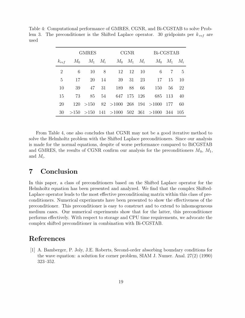
Table 4: Computational performance of GMRES, CGNR, and Bi-CGSTAB to solve Prob-lem 3. The preconditioner is the Shifted Laplace operator. 30 gridpoints per k ref areused

GMRES CGNR Bi-CGSTAB

kref M0 M1 Mi M0 M1 Mi M0 M1 Mi

2 6 10 8 12 12 10 6 7 5

5 17 20 14 39 31 23 17 15 10

10 39 47 31 189 88 66 150 56 22

15 73 85 54 647 175 126 685 113 40

20 120 >150 82 >1000 268 194 >1000 177 60

30 >150 >150 141 >1000 502 361 >1000 344 105

From Table 4, one also concludes that CGNR may not be a good iterative method tosolve the Helmholtz problem with the Shifted Laplace preconditioners. Since our analysisis made for the normal equations, despite of worse performance compared to BiCGSTABand GMRES, the results of CGNR confirm our analysis for the preconditioners M0, M1,and Mi.

7 Conclusion

In this paper, a class of preconditioners based on the Shifted Laplace operator for theHelmholtz equation has been presented and analyzed. We find that the complex Shifted-Laplace operator leads to the most effective preconditioning matrix within this class of pre-conditioners. Numerical experiments have been presented to show the effectiveness of thepreconditioner. This preconditioner is easy to construct and to extend to inhomogeneousmedium cases. Our numerical experiments show that for the latter, this preconditionerperforms effectively. With respect to storage and CPU time requirements, we advocate thecomplex shifted preconditioner in combination with Bi-CGSTAB.

References

[1] A. Bamberger, P. Joly, J.E. Roberts, Second-order absorbing boundary conditions forthe wave equation: a solution for corner problem, SIAM J. Numer. Anal. 27(2) (1990)323–352.

19

[2] A. Bayliss, C.I. Goldstein, E. Turkel, An iterative method for Helmholtz equation, J.Comput. Phys. 49 (1983) 443–457.

[3] R.W. Clayton, B. Engquist, Absorbing boundary conditions for wave-equation migra-tion, Geophysics 45(5) (1980) 895–904.

[4] B. Engquist, A. Majda, Absorbing boundary conditions for the numerical simulationof waves, Math. Comp. 31 (1977) 629–651.

[5] R. Fletcher, Conjugate gradient methods for indefinite systems, in: G.A. Watson,(Eds.), Proc. of the Dundee Biennal Conference on Numerical Analysis 1974, SpringerVerlag, New York, 1975, pp. 73–89.

[6] R.W. Freund, Preconditioning of symmetric, but highly indefinite linear systems, Num.Anal. Manus. 97-3-03, Bell Labs., Murray Hill, NJ, 1997.

[7] R.W. Freund, N.M. Nachtigal, QMR: a quasi minimum residual method for non-Hermitian Linear Systems, Numer. Math. 60 (1991) 315–339.

[8] M.J. Gander, F. Nataf, AILU for Helmholtz problems: a new preconditioner based onthe analytic parabolic factorization, J. Comp. Acoustics 9(4) (2001) 1499–1509.

[9] J. Gozani, A. Nachshon, E. Turkel, Conjugate gradient coupled with multigrid foran indefinite problem, in: Advances in Computer Methods for Partial DifferentialEquations V (1984) 425–427.

[10] N.J. Higham, Factorizing complex symmetric matrices with positive definite real andimaginary parts, Math. Comp. 67(3) (1998) 1591–1599.

[11] A.L. Laird, Preconditioned iterative solution of the 2D Helmholtz equation, FirstYear’s Report St. Hugh’s College (2001).

[12] M.M.M. Made, Incomplete factorization-based preconditionings for solving theHelmholtz equation, Int. J. Numer. Meth. Engng. 50 (2001) 1077–1101.

[13] C.C. Paige, M.A. Saunders, Solution of sparse indefinite systems of linear equations,SIAM J. Numer. Anal. 12 (4) (1975) 617–629.

[14] R.-E. Plessix, W.A. Mulder, Separation of variables as a preconditioner for an iterativeHelmholtz solver, To appear in Appl. Num. Math. (2003).

[15] Y. Saad, A flexible inner-outer preconditioned GMRES algorithm, SIAM J. Sci. Stat.Comput. 14 (1993) 461–469.

[16] Y. Saad, Iterative methods for sparse linear systems, PWS Publishing CompanyBoston, 1996.

20

[17] Y. Saad, M.H. Schultz, GMRES: A generalized minimal residual algorithm for solvingnonsymmetric linear systems, SIAM J. Sci. Stat. Comput. 7(12) (1986) 856–869.

[18] G.L.G. Sleijpen, J. Booten, D.R. Fokkema, H.A. van der Vorst, Jacobi-Davidson typemethods for generalized eigenproblems and polynomial eigenproblems, BIT 36 (1996)593–633.

[19] P. Sonneveld, CGS, a fast Lanczos-type solver for nonsymmetric linear systems, SIAMJ. Sci. Stat. Comput. 10 (1) (1986) 36–52.

[20] H.A. van der Vorst, Bi-CGSTAB: A fast and smoothly converging variant of BI-CGfor the solution of nonsymmetric linear systems, SIAM J. Sci. Stat. Comput. 13(2)(1992) 631–644.

[21] H.A. van der Vorst, J.B.M. Melissen, A Petrov-Galerkin type method for solvingAx = b, where A is symmetric complex, IEEE Trans. on Magnetics 26(2)(1990) 706–708.

[22] H.A. van der Vorst, C. Vuik, GMRESR: a family of nested GMRES methods, Num.Lin. Algebra Appl. 1(4) (1994) 369–386.

21