Seediscussions,stats,andauthorprofilesforthispublicationat:https://www.researchgate.net/publication/223649565

AcomparativestudybetweentwodifferentmethodsforsolvingthegeneralKorteweg–deVriesequation(GKdV)

ArticleinChaosSolitons&Fractals·August2007

DOI:10.1016/j.chaos.2006.11.011

CITATIONS

19

READS

210

2authors:

M.A.Helal

CairoUniversity

42PUBLICATIONS612CITATIONS

SEEPROFILE

MonaSamirMehanna

ModernTechnologyandInformationU…

5PUBLICATIONS120CITATIONS

SEEPROFILE

AllcontentfollowingthispagewasuploadedbyM.A.Helalon03December2016.

Theuserhasrequestedenhancementofthedownloadedfile.Allin-textreferencesunderlinedinblueareaddedtotheoriginaldocumentandarelinkedtopublicationsonResearchGate,lettingyouaccessandreadthemimmediately.

Chaos, Solitons and Fractals 33 (2007) 725–739

www.elsevier.com/locate/chaos

A comparative study between two different methods forsolving the general Korteweg–de Vries equation (GKdV)

M.A. Helal *, M.S. Mehanna

Department of Mathematics, Faculty of Science, University of Cairo, Giza, Cairo, Egypt

Accepted 10 November 2006

Abstract

The family of the KdV equations, the most famous equations embodying both nonlinearity and dispersion, hasattracted enormous attention over the years and has served as the model equation for the development of soliton the-ory. In this paper we present a comparative study between two different methods for solving the general KdV equation,namely the numerical Crank Nicolson method, and the semi-analytic Adomian decomposition method. The stability ofthe numerical Crank Nicolson scheme is discussed. A comparison between the two methods is carried out to illustratethe pertinent features of the two algorithms.� 2006 Elsevier Ltd. All rights reserved.

1. Introduction

Some physical properties of the solitary waves had been cited by Scott Russel in his report to the BritishAssociation in 1844. This can be found at an Internet page of the Herriot Watt University in Edinburgh (Scotland)[1].

The well known KdV equation had been derived in 1885 by the two scientists Korteweg and de Vries todescribe long wave propagation on shallow water. Although this equation was known since the last century, butits physical behaviour is still mysterious. The solitary waves represent the first and most celebrated solution tothe KdV equation. From a detailed numerical study, Zabusky and Kruskal [2] found that stable pulse like wavescould exist in a system described by the KdV equation. A remarkable quality of these solitary waves was that theycould collide with each other and yet preserve their shapes and speeds after the collision. This means that a col-lision between KdV solitary waves is elastic (i.e. the KdV equation is integrable). This particle like nature led Zabu-sky and Kruskal to name such waves solitons. The first presence of the soliton concept explained the recurrence inthe Fermi Pasta Ulam system. From numerical solution of the KdV equation with periodic boundary conditions(representing essentially a ring of coupled nonlinear springs), Zabusky and Kruskal [2] made the followingobservations. An initial profile representing a long wavelength excitation would ‘‘break up’’ into a number of

0960-0779/$ - see front matter � 2006 Elsevier Ltd. All rights reserved.doi:10.1016/j.chaos.2006.11.011

* Corresponding author. Tel.: +20 2 5676547.E-mail addresses: mahelal@yahoo.com (M.A. Helal), mona_mehanna@yahoo.com (M.S. Mehanna).

726 M.A. Helal, M.S. Mehanna / Chaos, Solitons and Fractals 33 (2007) 725–739

solitons, which would propagate around the system with different speeds. The solitons would collide but preservetheir individual shapes and speeds. During the past fifteen years a rather complete mathematical description ofsolitons has been developed.

The amount of information on nonlinear wave phenomena obtained through the fruitful collaboration of mathema-ticians and physicists using this description makes the soliton concept one of the most significant developments in mod-ern mathematical physics.

The nondispersive nature of the soliton solutions to the KdV equation arises not because the effects of dispersion areabsent but because they are balanced by nonlinearities in the system [3,4]. The classical Korteweg and de Vries (KdV)equation [5–9] arises in several areas of nonlinear physics (e.g., hydrodynamics, plasma physics, etc.). Earlier treatmentsby Karpman et al. [10] and Bisognano [11] have also developed theoretical models leading to the Korteweg deVriesequation for weakly nonlinear disturbances in neutral plasma loaded wave guides [10] and for intense beam propaga-tion in a circular pipe [11,12]. This equation has many other direct physical applications to solids, liquids, gases andplasma: magnetohydrodynamic waves in a cold plasma [13], longitudinal waves propagating in a one dimensional lat-tice of equal masses coupled by nonlinear springs, the Fermi et al. problem [14,15], ion acoustic waves in a cold plasma[16], rotating flow in tube [17] and longitudinal dispersive waves in elastic rods [18]. We refer the reader to Jeffrey andKakutani [19] and Miura [20] for more applications.

During the last five decades an exciting and extremely active area of research has been devoted to the construction ofexact solution for a wide class of nonlinear equations. This includes the most famous nonlinear one of Korteweg and deVries. In fact, it stimulated very important progress in the analytic treatment of initial value problems for nonlinearpartial differential equations describing wave propagation. Indeed, various branches of mathematics as well as physicshave been developed, renewed or even started to meet the needs of the nonlinear world.

Certain important and novel subareas of research leading to the construction of exact solutions such as the appli-cations of the Jacobian elliptic function [21], the powerful inverse scattering transform (IST), the B�acklund transforma-tions technique (BTs) [22,23], the Painleve analysis [24], the Lie group theoretical methods [25], the direct algebraicmethod [26] and tangent hyperbolic method [27].

Regarding formal mathematical approaches, Sawada and Kotera [28], Rosales [29], Whitham [30], Wadati and Saw-ada [31,32] and Hickernel [33] have all employed perturbation techniques. Their methods lead, after some tedious alge-braic manipulations, to the known N solitary wave solutions of some nonlinear partial differential equations, e.g. KdV,Burgers, Boussinesq equations etc.

In more recent work, Helal and El Eissa [34], Khater et al. [35,36] and Helal [37] have studied analytically andnumerically some physical problems that lead to the KdV equations and the soliton solutions have been obtained [38].

In the next order of the perturbation theory, a higher-order KdV equation can be obtained, which in general includescubic nonlinearity, fifth-order linear dispersion, and nonlinear dispersion. The contribution of the various high-orderterms depends on the parameters of the model (e.g. density stratification and shear flow), and sometimes several of themmay be more important.

The General Korteweg–de Vries equation (GKdV) has the following form:

ut � 6unux þ uxxx ¼ 0: ð1Þ

The second and third terms unux and uxxx represent the nonlinear convection and dispersion effects, respectively. Thesolitons of the GKdV equation arise as a balance between nonlinear convection and dispersion terms. The nonlineareffect causes the steepening of waveform [32], while the dispersion effect makes the waveform spread. Due to the com-petition of these two effects, a stationary waveform (solitary wave) exists. The reason why each solitary wave is stable inspite of mutual interactions is that the GKdV equation has an infinite number of conserved quantities. Dynamical prop-erties of the system are severely restricted by the existence of an infinite number of conservation laws. The conservedquantities guarantee the time-independence of parameters which characterize the solitons, and therefore the solitons arestable. Corresponding to an infinite number of conserved quantities (recall the field variable has infinite degrees of free-dom), arbitrary number of solitons may coexist [39].

One of the most important special case of the General Korteweg–de Vries equation (GKdV) is the modified Kor-teweg de Vries (mKdV) equation. This equation is derived by setting n = 2 in the GKdV equation. It has many physicalapplications as well . These applications include electrodynamics, electromagnetic waves in size-quantised films, internalwaves for certain special density stratifications, elastic media, and traffic flow. The mKdV equation occurs in two ver-sions; the cubic nonlinearity term can have either positive or negative sign. Hirota [40] found the N soliton solution forthe version of the mKdV equation with positive sign. Both Perelman et al. [41] and Ono [42] developed the N solitonsolution for the case with negative sign. Of particular interest in the negative case is the elastic interaction of a solitonwith a dissipationless shock wave [43].

M.A. Helal, M.S. Mehanna / Chaos, Solitons and Fractals 33 (2007) 725–739 727

Another important special cases of the nonlinear partial differential equation is the extended Korteweg–de Vries(eKdV) equation, sometimes called as the Gardner equation, which has the form:

ut þ auux þ bu2ux þ uxxx ¼ 0: ð2Þ

This equation has been used as a model of strongly nonlinear internal waves in the ocean [44]. The coefficient b ofthe cubic nonlinear term may take the positive or negative sign, depending on the fluid stratification. For the classicaltwo layer model it is always negative, but for certain three layer models, it may be negative, or positive, or zero [45].The solutions of the eKdV equation describe various kinds of nonlinear waves (solitons, breathers, dissipationlessshock waves) for the various signs of the coefficients (a,b) of the quadratic and cubic nonlinear terms. A knowledgeof possible wave regimes is very important for an understanding of nonlinear wave dynamics in the ocean and atmo-sphere [46].

The basic motivation of this work to approach the General KdV equation differently, but effectively, by using analternative techniques. In this work, we will use two different methods: the first one is the Adomian decompositionmethod [47–55] in a direct manner. The introduction of this algorithm not only provides the solution in a rapidly con-vergent series [47–55], but it also guarantees considerable savings of the calculations size, the second method used is theFinite difference technique that will be applied to handle our study numerically. More details and examples can befound in the last section.

2. Exact solution

The general KdV equation is presented by the following equation:

ut þ 6unux þ uxxx ¼ 0; ð3Þ

where u = u(x, t) is the wave function. Specific exact solution will be determined for each value of n given by,

n

u(x, t)

1

c 2

ffiffifficp

sech

se

ð Þ4s

ð Þ5s

ð3Þ

ð2ðx� ctÞÞ;

hðffiffifficpðx� ctÞÞ;

2

2 ffiffifficp

sec

ffiffiffip

3 ffiffiffiffiffi5c3

r2 3

ch3ð2

cðx� ctÞÞ;

12

ffiffiffip

4 2

5c 1

ech ð2 cðx� ctÞÞ;

2 5 ffiffiffip

5 27c 1

ech5ð2

cðx� ctÞÞ;

1 1 ffiffiffip

6 214c

6sech3ð3 cðx� ctÞÞ;

where c is the velocity of the wavefront.

3. The finite-difference method

The most suitable finite-difference method for solving the nonlinear partial differential equation is Crank–Nicolsonmethod. In order to solve Eq. (3) numerically, both space and time are divided into a large numbers of grid points andderivatives are replaced by finite-difference approximations.

Let h and k be the step sizes in coordinate and time grids and n the number of grid points in coordinate grid. The gridpoints (xi, tj) are given by:

xi ¼ ih; for i ¼ 0; 1; . . . ; n and tj ¼ jk; for j P 0

The method is based on replacing ux, uxxx by the mean of there finite-difference representations on the (j + 1)th andjth time rows and approximates Eq. (3) by

728 M.A. Helal, M.S. Mehanna / Chaos, Solitons and Fractals 33 (2007) 725–739

r4

uiþ2;jþ1 þr2ð3h2un � 1Þuiþ1;jþ1 þ ui;jþ1 þ

r2ð1� 3h2unÞui�1;jþ1 �

r4

ui�2;jþ1

¼ �r4

uiþ2;j þr2ð1� 3h2unÞuiþ1;j þ ui;j þ

r2ð3h2un � 1Þui�1;j þ

r4

ui�2;j; ð4Þ

where r ¼ kh3 ; i ¼ 1; 2; . . . ; n, and j P 1.

3.1. Stability analysis

Applying the Von Neumann stability technique in Eq. (4), we find that the scheme is unconditionally stable. Thisleads to the confirmation that, the numerical error will not grow for subsequent marching step in t, and the numericalsolution will proceed in a stable manner.

3.2. Consistency

The difference equation is consistent with the differential equation if the limiting value of the local truncation errortends to zero as h! 0, k! 0. To discuss the consistency of this scheme with the partial differential equation, we expandthe terms

uiþ2;jþ1; uiþ1;jþ1; ui;jþ1; ui�1;jþ1; ui�2;jþ1; uiþ2;j; uiþ1;j; ui�1;j; ui�2;j

about the point (ih, jk) by Taylor’s series, this leads to the following truncation error:

T i;j ¼ k2 1

2uxxxt þ 3unuxt þ

1

2utt

� �þ k3 1

4uxxxtt þ

3

2unuxtt þ

1

6uttt

� �þ kh2 4

15uxxxxx þ unuxxx

� �þ � � �

which tends to zero as h and k tends to zero. Hence the finite-difference equation is consistent with the differentialequation.

4. The decomposition method

To begin with, Eq. (3) can be written in an operator form

Lu ¼ �6unux � uxxx;

uðx; 0Þ ¼ f ðxÞ;ð5Þ

where the differential operator L is

L � o

otð6Þ

and the inverse operator L�1 is an integral operator given by

L�1ð�Þ ¼Z t

0

ð�Þdt: ð7Þ

The Adomian decomposition method [47,49] assumes a series solution for the unknown function u(x, t) given by

uðx; tÞ ¼X1n¼0

unðx; tÞ; ð8Þ

and the nonlinear term F(u) = unux can be decomposed into an infinite series of polynomials given by

F ðuÞ ¼X1n¼0

An; ð9Þ

where the components un(x, t) will be determined recurrently, and An are the so called Adomian polynomials ofu0,u1,u2, . . . ,un defined by

An ¼1

n!

dn

dkn FX1i¼0

kiui

!" #k¼0

ð10Þ

M.A. Helal, M.S. Mehanna / Chaos, Solitons and Fractals 33 (2007) 725–739 729

These polynomials can be calculated for all classes of nonlinearity according to algorithms given by Adomian [47,48]and recently, an alternative approach was developed by Wazwaz [49].

Operating with the integral operator L�1 on both sides of (5) and using the initial condition, we find

uðx; tÞ ¼ f ðxÞ þ L�1ð�6unux � uxxxÞ ð11Þ

Substituting (8) and (9) into the functional equation (11) yields

X1n¼0

unðx; tÞ ¼ f ðxÞ þ L�1 �6X1n¼0

An

!�

X1n¼0

un

!xxx

!ð12Þ

The Adomian method admits that the zeroth component u0(x, t) be identified by all terms that arise from the initialconditions and from the source terms if exist, and as a result, the remaining components un(x, t),n P 1 can be deter-mined by using the recurrence relation

u0ðx; tÞ ¼ f ðxÞ;ukþ1ðx; tÞ ¼ Lð�6Ak � ðukÞxxxÞ; k P 0;

ð13Þ

where Ak, k P 0 are Adomian polynomials that represent the nonlinear term (unux) and given by

A0 ¼ un0u0x;

A1 ¼ nun�10 u0xu1 þ un

0u1x;

A2 ¼ nun�10 u1u1x þ

1

2nðn� 1Þu0xun�2

0 u21 þ nu0xun�1

0 u2 þ un0u2x;

A3 ¼1

2nðn� 1Þun�2

0 u1xu21 þ nðn� 1Þu0xun�2

0 u1u2 þ nun�10 u1u2x þ nun�1

0 u1xu2;

þ 1

6nðn� 1Þðn� 2Þu0xun�3

0 u31 þ nu0xun�1

0 u3 þ un0u3x:

ð14Þ

Other polynomials can be generated in a like manner.The first few components of un(x, t) follow immediately upon setting:

u0ðx; tÞ ¼ f ðxÞ;u1ðx; tÞ ¼ L�1ð�6A0 � ðu0ÞxxxÞ;u2ðx; tÞ ¼ L�1ð�6A1 � ðu1ÞxxxÞ;u3ðx; tÞ ¼ L�1ð�6A2 � ðu2ÞxxxÞ;u4ðx; tÞ ¼ L�1ð�6A3 � ðu3ÞxxxÞ:

ð15Þ

The scheme in (15) can easily determine the components un(x, t), n � 0. It is, in principle, possible to calculate morecomponents in the decomposition series to enhance the approximation. Consequently, one can recursively determineevery term of the series

P1n¼0unðx; tÞ, and hence the solution u(x, t) is readily obtained in a series form. It is interesting

to note that we obtained the series solution by using the initial condition only. The obtained series may lead to the exactsolution.

5. Convergence results

The convergence of the decomposition series have been investigated by several authors [56–58]. In this work, we willdiscuss the convergence analysis [59] of the Adomian decomposition method.

Consider a Hilbert space H,(., .) with the scalar product in H and kÆk the associated norm, defined by:H = L2((a,b) · [0,T]) the set of applications:

u : ða; bÞ � ½0; T � ! R with

Zða;bÞ�½0;T �

u2ðx; sÞdsds < þ1

and the following represent the scalar product:

ðu; vÞH ¼Zða;bÞ�½0;T �

uðx; sÞvðx; sÞdsds

730 M.A. Helal, M.S. Mehanna / Chaos, Solitons and Fractals 33 (2007) 725–739

and

If N i

kuk2H ¼

Zða;bÞ�½0;T �

u2ðx; sÞdsds

is the associated norm.Let us write our problem in an operator form:

Luþ Ruþ Nu ¼ 0;

whereL: is a differential operator defined by: L � o

otR: the remainder of the linear operatorN: the nonlinear operator

Let T be an operator defined by:

Tu ¼ �Ru� Nu

We consider the following hypotheses:

(H1) (T(u) � T(v),u � v) P kku � vk2; k > 0, "u,v 2 H

(H2) whatever may be M > 0, there exists a constant C(M) > 0 such that for u,v 2 H with kuk 6M, kvk < M, we have:

ðT ðuÞ � T ðvÞ;wÞ 6 CðMÞku� vkkwk for every w 2 H

With the above hypotheses (H1) and (H2), Cherruault [58], Mavoungou and Cherrulaut [57] have proved con-vergence of the method by using ideas developed by Sibony [58] when applied to general partial differentialequations.

Theorem (Sufficient condition of convergence).

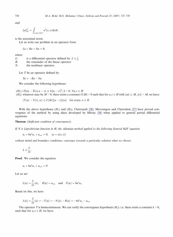
s Lipschitizian function in H, the Adomian method applied to the following General KdV equation

ut þ 6unux þ uxxx ¼ 0; ðu ¼ uðx; tÞÞ

without initial and boundary conditions, converges towards a particular solution when we choose:

L � o

ot:

Proof. We consider the equation

ut þ 6unux þ uxxx ¼ 0

Let us set:

LðuÞ ¼ o

otðuÞ; RðuÞ ¼ uxxx and NðuÞ ¼ 6unux:

Based on this, we have

LðuÞ ¼ o

otðuÞ ¼ �T ðuÞ ¼ �NðuÞ � RðuÞ ¼ �6unux � uxxx

The operator T is hemicontinuous. We can verify the convergence hypothesis (H1): i.e. there exists a constant k > 0,such that for u,v 2 H, we have:

M.A. Helal, M.S. Mehanna / Chaos, Solitons and Fractals 33 (2007) 725–739 731

ðT ðuÞ � T ðvÞ; u� vÞP kku� vk2;

T ðuÞ � T ðvÞ ¼ 6un ouox� 6vn ov

ox

� �þ o3u

ox3� o3v

ox3

� �

¼ 6

nþ 1

o

oxðunþ1 � vnþ1Þ þ o3

ox3ðu� vÞ;

ðT ðuÞ � T ðvÞ; u� vÞ ¼ 6

nþ 1

o

oxðunþ1 � vnþ1Þ; u� v

� �þ o3

ox3ðu� vÞ; u� v

� �:

Notice that oox ;

o3

ox3 are differential operators in H, then there exist real constants d1,d2 > 0 such that

o

oxðunþ1 � vnþ1Þ; u� v

� �6 d1kunþ1 � vnþ1k � ku� vk

6 d1kðu� vÞðun þ un�1vþ un�2v2 þ un�3v3 þ � � � þ vnÞk � ku� vk6 d1ku� vk � kun þ un�1vþ un�2v2 þ un�3v3 þ � � � þ vnk � ku� vk6 ðnþ 1Þd1Mnku� vk2

� o

oxðunþ1 � vnþ1Þ; u� v

� �P ðnþ 1Þd1Mnku� vk2

;

where kuk 6M, kvk 6M.Similarly

o3

ox3ðu� vÞ; u� v

� �6 d2kðu� vÞk � ku� vk

6 d2ku� vk2;

� o3

ox3ðu� vÞ; u� v

� �P d2kðu� vÞk2

;

ðT ðuÞ � T ðvÞ; u� vÞP �61

ðnþ 1Þ ðnþ 1Þd1Mnku� vk2

� �� d2ku� vk2 ¼ Kku� vk2

Setting: K = �6d1Mn � d2, then we obtain hypothesis (H1).We can prove the hypothesis (H2), i.e. "M > 0, $C(M) > 0 such that kuk 6M, kvk 6M)

(T(u) � T(v),w) 6 C(M)ku � vkkwk, "w 2 H.Thus we have:

ðT ðuÞ � T ðvÞ;wÞ ¼ 61

nþ 1

o

oxðunþ1 � vnþ1Þ;w

� �þ o3

ox3ðu� vÞ;w

� �

6 61

ðnþ 1Þ ðnþ 1ÞMnku� vkkwk þ ku� vkkwk;¼ ð6Mn þ 1Þku� vkkwk ¼ CðMÞku� vkkwk;

where C(M) = 6Mn + 1. Hence, the hypothesis (H2) is satisfied. h

6. Application

Consider the initial value problem associated with the General KdV equation:

ut þ 6unux þ uxxx ¼ 0

using the initial condition

732 M.A. Helal, M.S. Mehanna / Chaos, Solitons and Fractals 33 (2007) 725–739

for n ¼ 1; uðx; 0Þ ¼ c2

sech2

ffiffifficp

2x

� �;

for n ¼ 2; uðx; 0Þ ¼ffiffifficp

sechffiffifficp

x� �

;

for n ¼ 3; uðx; 0Þ ¼ffiffiffiffiffi5c3

3

rsech

23

3

2

ffiffifficp

x� �

;

for n ¼ 4; uðx; 0Þ ¼ 5c2

� �14

sech12 2

ffiffifficp

x� �

;

for n ¼ 5; uðx; 0Þ ¼ 7c2

� �15

sech25

5

2

ffiffifficp

x� �

;

for n ¼ 6; uðx; 0Þ ¼ 14c3

� �16

sech13ð3

ffiffifficp

xÞ;

ð16Þ

with u = u(x, t) is a sufficiently smooth function, and f(x) is bounded. As indicated before, we shall assume that the solu-tion u(x, t), along with its derivatives, tends to zero as jxj ! 1.

Applying the inverse operator L�1 on both sides of (3) yield Eq. (12), Adomian decomposition method [47,49] givesthe recurrence relation (13) as we mentioned before.

The solution in series form is

n ¼ 1

uðx; tÞ ¼ 1

2sech

x2

h i2

þ 1

8t2ð�2þ cosh½x�Þsech

x2

h i4

þ 1

384t4ð33� 26 cosh½x�

þ cosh½2x�Þsechx2

h i6

þ 1

48t3 sech

x2

h i5

sinh3x2

� �þ 1

2t sech

x2

h i2

tanhx2

h i

� 11

48t3 sech

x2

h i4

tanhx2

h iþ � � �

n ¼ 2

uðx; tÞ ¼ sech½x� þ 1

2t2 sech½x� � t2 sech½x�3 þ 1

192t4ð115� 76 cosh½2x� þ cosh½4x�Þ

� sech½x�5 þ 1

24t3 sech½x�4 sinh½3x� þ t sech½x� tanh½x� � 23

24t3 sech½x�3 tanh½x� þ � � �

n ¼ 3

uðx; tÞ ¼ 5

3

� �13

sech3x2

� �23

þ 1

4

5

3

� �13

t2ð�4þ cosh½3x�Þsech3x2

� �83

þ 1

192

5

3

� �13

t4

� ð273� 166 cosh½3x� þ cosh½6x�Þsech3x2

� �143

þ 5

3

� �13

t sech3x2

� �53

sinh3x2

� �

þ 1

24

5

3

� �13

t3 sech3x2

� �11

3�39 sinh

3x2

� �þ sinh

9x2

� �� �þ � � �

n ¼ 4 ð18Þ

uðx; tÞ ¼ 5

2

� �14 ffiffiffiffiffiffiffiffiffiffiffiffiffiffiffiffi

sech½2x�p

þ 1

4

5

2

� �14

t2ð�5þ cosh½4x�Þsech½2x�52 þ 1

192

5

2

� �14

t4

� ð531� 308 cosh½4x� þ cosh½8x�Þsech½2x�92 þ 5

2

� �14

t sech½2x�32 sinh½2x�

þ 1

24

5

2

� �14

t3 sech½2x�72ð�59 sinh½2x� þ sinh½6x�Þ þ � � �

M.A. Helal, M.S. Mehanna / Chaos, Solitons and Fractals 33 (2007) 725–739 733

n ¼ 5

uðx; tÞ ¼ 7

2

� �15

sech5x2

� �25

þ 1

4

7

2

� �15

t2ð�6þ cosh½5x�Þsech5x2

� �125

þ 1

192

7

5

� �15

t4

� ð913� 514 cosh½5x� þ cosh½10x�Þsech5x2

� �225

þ 7

2

� �15

t sech5x2

� �75

sinh5x2

� �

þ 1

24

7

2

� �15

t3sech5x2

� �175

�83 sinh5x2

� �þ sinh

15x2

� �� �þ � � �

n ¼ 6

uðx; tÞ ¼ 14

3

� �16

sech½3x�13 þ

73

� �16t2ð�7þ cosh½6x�Þsech½3x�

73

2256

þ 1

96256

7

3

� �16

t4

� ð1443� 796 cosh½6x� þ cosh½12x�Þsech½3x�133

!þ 14

3

� �16

t sech½3x�43 sinh½3x�

þ73

� �16t3ð�55þ cosh½6x�Þsech½3x�

103 sinh½3x�

6256

þ � � �

The previous solutions are the series solutions for the exact solutions given before. This means that these series willconverge to the exact solutions given in closed forms.

When we replace the non linear term (unux) by the term (auux � bu2ux) (containing the summation of u with twodifferent powers) , we obtain the well known equation ‘‘the Gardner equation or the combined KdV–mKdV equation’’.It has an infinite number of solutions. The equation has the form

ut þ auux � bu2ux þ uxxx ¼ 0; b > 0 ð19Þ

With exact solution

uðx; tÞ ¼ a2b

1 tanha

2ffiffiffiffiffiffi6bp x� a2

6bt

� �� �� �ð19iÞ

having the following Numerical scheme:

r4

uiþ2;jþ1 þr4ðh2ðau� bu2Þ � 2Þuiþ1;jþ1 þ ui;jþ1 þ

r4ð2� h2ðau� bu2ÞÞui�1;jþ1 �

r4

ui�2;jþ1

r4

uiþ2;j

þ r4ðh2ðau� bu2Þ � 2Þuiþ1;j � ui;j þ

r4ð2� h2ðau� bu2ÞÞui�1;j �

r4

ui�2;j ¼ 0

with the same condition of stability and consistency. But the convergence results for Adomian decomposition will differ,and given by

T ðuÞ ¼ auux � bu2ux þ uxxx

ðT ðuÞ � T ðvÞÞ ¼ auouox� av

ovox

� �� bu2 ou

ox� bv2 ov

ox

� �þ o3u

ox3� o3u

ox3

� �

¼ a2

o

oxðu2 � v2Þ � b

3

o

oxðu3 � v3Þ þ o3

ox3ðu� vÞ:

Recall that oox ;

o3

ox3 are differential operator in H, then there exist real constants d1,d2,d3 > 0 such thatAccording to Schwartz inequality, we have:

o

oxðu2 � v2Þ; u� v

� �6 d1ku2 � v2k � ku� vk 6 d1kðu� vÞðuþ vÞk � ku� vk 6 d1ð2MÞku� vk2

;

� o

oxðu2 � v2Þ; u� v

� �P 2Md1ku� vk2

;

o

oxðu3 � v3Þ; u� v

� �6 d2ku3 � v3k � ku� vk 6 d2kðu� vÞðu2 þ uvþ v2Þk � ku� vk 6 d2ð3M2Þku� vk2

;

� o

oxðu3 � v3Þ; u� v

� �P 3M2d2ku� vk2

:

734 M.A. Helal, M.S. Mehanna / Chaos, Solitons and Fractals 33 (2007) 725–739

As calculated before

TableErrors

h = 0.1

x

1234567

� o3

ox3ðu� vÞ; u� v

� �P d3ku� vk2;

ðT ðuÞ � T ðvÞ; u� vÞP � a2� 2Md1ku� vk2 þ b

3� 3M2d2ku� vk2 � d3ku� vk2 ¼ Kku� vk2

;

Setting: K = �ad1M + bd2M2 � d3, then we obtain hypothesis (H1).We next can prove the hypothesis (H2),

ðT ðuÞ � T ðvÞ;wÞ ¼ a2

o

oxðu2 � v2Þ;w

� �� b

3

o

oxðu3 � v3Þ;w

� �þ o3

ox3ðu� vÞ;w

� �6 aMku� vkkwk � bM2ku� vkkwk þ ku� vkkwk ¼ ð�bM2 þ aM þ 1Þku� vkkwk¼ CðMÞku� vkkwk;

where C(M) = �bM2 + aM + 1.Hence, the hypothesis (H2) is satisfied.Ak, Bk are the Adomian polynomials that represent the nonlinear terms (auux) and (bu2ux) respectively, are given by

A0 ¼ au0u0x;

A1 ¼ au0u1x þ au1u0x;

A2 ¼ au0u2x þ au1u1x þ au2u0x;

A3 ¼ au0u3x þ au3u0x þ au1u2x þ au2u1x;

ð20iÞ

B0 ¼ bu20u0x;

B1 ¼ bu20u1x þ 2bu0u1u0x;

B2 ¼ bu20u2x þ 2bu0u1u1x þ bu2

1u0x þ 2bu0u2u0x;

B3 ¼ bu20u3x þ 2bu0u3u0x þ bu2

1u1x þ 2bu0u2u1x þ 2bu1u2u0x þ 2bu0u1u2x:

ð20iiÞ

the solution in a series form is thus given by

uðx; tÞ ¼ta4sech xa

2ffiffi6p ffiffi

bp

� �2

24ffiffiffi6p

b52

�t3a10 �2þ cosh xaffiffi

6p ffiffi

bp

� �� �sech xa

2ffiffi6p ffiffi

bp

� �4

62208ffiffiffi6p

b112

�t2a7sech xa

2ffiffi6p ffiffi

bp

� �2

tanh xa

2ffiffi6p ffiffi

bp

� �1728b4

� 1

8957952b7t4a13 �5þ cosh

xaffiffiffi6p ffiffiffi

bp

� �� �sech

xa

2ffiffiffi6p ffiffiffi

bp

� �4

tanhxa

2ffiffiffi6p ffiffiffi

bp

� � !

þa 2þ tanh xa

2ffiffi6p ffiffi

bp

� �� �2b

þ � � � ð21Þ

it is obvious now that the last series solution leads to the exact solution given above in (19i).

1afounded by using ADM and CN compared to the exact solution of the GKdV equation for n = 1,2

t = 0.005

uexact � uCN uexact � uADM uexact � uCN uexact � uADM

n = 1 n = 1 n = 2 n = 2

�0.0000557264 1.45994E�14 6.07153E�18 �3.87468E�14�5.68516E�06 �5.57887E�15 5.20417E�18 �1.7708E�14�8.55601E�07 �2.08167E�15 3.46945E�18 1.06859E�15

6.28982E�08 2.08167E�17 3.46945E�18 8.74301E�16�2.72279E�07 2.08167E�16 �4.33681E�18 3.48679E�16�0.0000591607 1.0842E�16 �1.0842E�17 1.2837E�16

0 4.40186E�17 0.0 4.74881E�17

Table 1bErrors founded by using ADM and CN compared to the exact solution of the GKdV equation for n = 3,4

h = 0.1 t = 0.005

x uexact � uCN uexact � uADM uexact � uCN uexact � uADM

n = 3 n = 3 n = 4 n = 4

1 2.1684E�19 �2.71227E�13 1.19262E�17 �3.56604E�132 �8.0231E�18 �4.27436E�15 2.55872E�17 2.94209E�153 �1.14925E�17 2.26208E�15 2.25514E�17 2.27596E�154 �1.14925E�17 8.95117E�16 2.25514E�17 8.46545E�165 �6.93889E�18 3.36536E�16 2.38524E�17 3.10516E�166 �2.60209E�18 1.21431E�16 2.08167E�17 1.14492E�167 0.0 4.53197E�17 0.0 4.22839E�17

Table 1cErrors founded by using ADM and CN compared to the exact solution of the GKdV equation for n = 5,6

h = 0.1 t = 0.005

x uexact � uCN uexact � uADM uexact � uCN uexact � uADM

n = 5 n = 5 n = 6 n = 6

1 �2.81893E�18 �2.9332E�13 �9.97466E�18 �1.944E�132 �8.89046E�18 5.10703E�15 �6.28837E�18 5.52336E�153 �4.11997E�18 2.19269E�15 �2.1684E�19 2.10942E�154 �6.50521E�18 8.01442E�16 �2.1684E�19 7.84095E�165 5.85469E�18 2.94903E�16 0.0 2.87964E�166 6.50521E�19 1.0842E�16 �2.1684E�18 1.06685E�167 0.0 3.9465E�17 0.0 3.88144E�17

Table 2aErrors founded by using ADM and CN compared to the exact solution of the Gardner equation for: (a = 0.1, b = 0.9) and (a = 0.4,b = 0.6)

h = 0.1 t = 0.005

n = 1 and n = 2 (Gardner equation)

x uexact � uCN uexact � uADM uexact � uCN uexact � uADM

a = 0.1 b = 0.9 a = 0.4 b = 0.6

1 �0.000166875 6.93889E�18 �0.00490656 �5.55112E�172 �0.0000249649 0 �0.000733026 �5.55111E�173 �1.20185E�7 0 �3.52548E�6 04 1.13298E�12 0 �5.91205E�10 �5.55112E�175 2.44227E�7 6.93889E�18 4.45074E�6 �1.11022E�166 0.0000379774 0 0.000692143 �2.22045E�167 0 0 0 �1.11022E�16

Table 2bErrors founded by using ADM and CN compared to the exact solution of the Gardner equation for: a = 0.8, b = 0.2

h = 0.1 t = 0.005

n = 1 and n = 2 (Gardner equation)

x uexact � uCN uexact � uADM

a = 0.8 b = 0.2

1 �0.102342 �4.44089E�162 �0.0150857 03 �0.0000715515 4.44089E�164 �1.91758E�8 �4.44089E�165 3.5334E�6 �4.44089E�166 0.000565815 07 0 �4.44089E�16

M.A. Helal, M.S. Mehanna / Chaos, Solitons and Fractals 33 (2007) 725–739 735

Fig. 1. Approximation of u(x, t) obtained by using the ADM for time t = 0.005.

736 M.A. Helal, M.S. Mehanna / Chaos, Solitons and Fractals 33 (2007) 725–739

7. Numerical results and some illustrations

In what follows, we present the errors that result from using Adomian decomposition method (ADM) and the CrankNicolson method (CN) (Tables 1 and 2).

Where error = exact value � approximated value.

Fig. 2. Approximation of u(x, t) obtained by using the ADM for time 0.005 6 t.

Fig. 3. (a)–(c) Approximation of u(x, t) obtained by using the ADM for time t = 0.005.

M.A. Helal, M.S. Mehanna / Chaos, Solitons and Fractals 33 (2007) 725–739 737

Fig. 1 shows the soliton solution (18) of the GKdV equation for n = 1, 2, and 3 on the left, n = 4, 5 and 6 on theright, t = 0.005 and �6 6 x 6 6.

Fig. 2 shows the soliton solution (18) of the GKdV equation for n = 1, 2, 3, 4, 5 and 6, 0.005 6 t 6 0.01 and�10 6 x 6 10.

Fig. 3(a)–(c) show the soliton solution (21) of the Gardner equation using an alternative values for a,b, t = 0 0.005and �6 6 x 6 6.

8. Conclusion

The main goal of this work is to conduct a comparative study between two methods, the first is a pure numericalmethod, and the second is a semi-analytical method. To achieve our goal, we applied the two methods to the GKdVequation and the Gardner equation. We carried out our analysis by using the two methods. The series solutions were

738 M.A. Helal, M.S. Mehanna / Chaos, Solitons and Fractals 33 (2007) 725–739

obtained that can lead to the closed form solution. Tables that show errors between the exact results and the obtainedapproximations were presented. The tables clearly show that the Adomian method works effectively for numerical pur-poses, and it gives results of higher accuracy level compared to the traditional Crank Nicolson method. Graphs of thesolitons solutions of these well known nonlinear wave equations were also given to support analysis. The stability of thesolutions were investigated as well.

The approximation can be obtained to any desired number of terms to enhance the accuracy level.There is an important point to make here. Unlike the perturbation technique, where the complexity of the calcula-

tions increases rapidly with the increase of order of terms, the Adomian method leads to approximation through areduced size of calculations. The advantage of using the Adomian decomposition method demonstrates the reliabilityand the efficiency of this work.

The comparison of the numerical results was done between the decomposition method, Crank–Nicolson method andthe exact solution in Tables 1 and 2. The decomposition method is numerically more accurate than the conventionalnumerical method of the Crank Nicolson, and it is also easier to use.

References

[1] Eilbeck, C. 1998. http://www.ma.hw.ac.uk/chris/scott_russell.html.[2] Zabusky NJ, Kruskal MD. Interaction of solitons in a collisionless plasma and the recurrence of initial states. Phys Rev Lett

1965;15:240–3.[3] Dodd RK, Eilbeck JC, Gibbon JD, Morris HC. Solitons and nonlinear wave equations. New York: Academic Press; 1982.[4] Lomdahl PS. What is a soliton? Los Alamos Science Spring, 1984. p. 27–31.[5] Korteweg DJ, de Vries G. Philos Mag 1895;39:422.[6] Washimi H, Taniuti T. Phys Rev Lett 1966;17:966.[7] Gardner CS, Greene JM, Kruskal MD, Miura RM. Phys Rev Lett 1967;19:1095.[8] Ott E, Sudan RN. Phys Fluids 1969;12:2388.[9] Davidson RC. Methods in nonlinear plasma theory. New York: Academic Press; 1972.

[10] Karpman VI, Lynov JP, Michelsen P, Pecseli HL, Rasmussen JJ, Turikov VA. Phys Fluids 1980;23:1782.[11] Bisognano JJ. In: Proceedings of the 1996 European particle accelerator conference, Sitges. Bristol, UK: IOP; 1996. p. 328–30.[12] Davidson Ronald C. Korteweg–deVries equation for longitudinal disturbances in coasting charged-particle beams. Physical

Review special topics—accelerators and beams 2004;7:054402-1–2-5.[13] Gardner CS, Morikawa GK. Similarity in the asymptotic behavior of collision-free hydromagnetic waves and water waves. New

York Univ., Courant Inst. Math. Sci. Res. Rep. NYO-9082, 1960.[14] Fermi E, Pasta J, Ulam S. Studies of nonlinear problems, I. Los Alamos Report LA 1940; 1955.[15] Kruskal MD, Zabusky NJ. Progress on the Fermi–Pasta–Ulam nonlinear string problem. Princeton Plasma Physics Laboratory

Annual Rep. MATT-Q-21, Princeton, NJ, 1963. p. 301–308.[16] Taniuti T, Washimi H. Propagation of ion-acoustic solitary waves of small amplitude. Phys Rev Lett 1966;17:996–8.[17] Leibovich S. Weakly non-linear waves in rotating fluids. J Fluid Mech 1970;42:803–22.[18] Nariboli GA. Nonlinear longitudinal dispersive waves in elastic rods. Iowa State Univ. Engineering Res. Inst Preprint, 1969. p.

442 .[19] Jeffrey A, Kakutani T. Weak nonlinear dispersive waves: a discussion centred around the Korteweg–de Vries. SIAM Rev

1972;14:582.[20] Miura RM. The Korteweg–de Vries equation: a survey of results. SIAM Rev 1976;18:412–59.[21] Lamb GL. Elements of soliton theory. New York: Wiley; 1980.[22] Khater AH, Helal MA, El Kalaawy OH. Backlund transformations: exact solutions for the KdV and Calogero–Degasperis–Fokas

mKdV equations. Math Meth Appl Sci 1998;21:719–31.[23] Wahlquist HD, Estabrook FB. Backlund transformation for solutions of the KdV equation. Phys Rev Lett 1973;31:1386–90.[24] Khater AH, El-Sabbagh MF. The Painleve property and coordinates transformations. Nuovo Cimento B 1989;104(2):123–9.[25] Olver PJ. Applications of Lie groups to differential equations. Graduate texts in mathematics. Berlin: Springer; 1986.[26] Hereman W, Korpel A, Banerjee PP. A general physical approach to solitary wave construction from linear solutions. Wave

Motion 1985;7(3):283–9.[27] Malfliet W. Solitary wave solutions of nonlinear wave equations. Am J Phys 1992;60(7):650–4.[28] Sawada K, Kotera T. A method for finding N-Solitons of the KdV equation and KdV like equation. Prog Theor Phys

1974;51:1355–67.[29] Rosales RR. Exact solutions of some nonlinear evolution equations. Stud Appl Math 1978;59:117–57.[30] Whitham GB. Linear and nonlinear waves. New York: Wiley/Interscience; 1974.[31] Wadati M, Sawada K. New representations of the soliton solution for the KdV equation. J Phys Soc Jpn 1980;48:312–8.[32] Wadati M, Sawada K. Application of the trace method to the modified KdV equation. J Phys Soc Jpn 1980;48:319–26.[33] Hickernel FJ. The evolution of large horizontal scale disturbance in marginally stable, inviscid, shear flows: II. Solution of the

Boussinesq equation. Stud Appl Math 1983;69:23–49.

M.A. Helal, M.S. Mehanna / Chaos, Solitons and Fractals 33 (2007) 725–739 739

[34] Helal MA, El Eissa HN. Shallow water waves and KdV equation (oceanographic application). PUMA 1996;7(3–4):263–82.[35] Khater AH, El- Kalaawy OH, Helal MA. Two new classes of exact solutions for the KdV equation via Backlund transformations.

Chaos, Solitons & Fractals 1997;8(12):1901–9.[36] Khater AH, Helal MA, Seadawy AR. General soliton solutions of an n-dimensional nonlinear Schrodinger equation. Nuovo

Cimento B 2000;115(11):1303–11.[37] Helal MA. Chebyshev spectral method for solving KdV equation with hydro dynamical application. Chaos, Solitons & Fractals

2001;12:943–50.[38] Helal MA. Soliton solution of some nonlinear partial differential equations and its applications in fluid mechanics. Chaos, Solitons

& Fractals 2002;13:1917–29.[39] Wadati M. Introduction to solitons. Pramana J Phys 2001;57(5 & 6):841–7.[40] Hirota R. J Phys Soc Jpn 1972;33:1456.[41] Perelman TL, Fridman AK, El’yashevich MM. Phys Lett 1974;47B:321.[42] Ono H. J Phys Soc Jpn 1976;40:1487.[43] Marchant TR. Asymptotic solitons for a higher-order modified Korteweg de Vries equation. Phys Rev E 2002;66:046623-1–3-8.[44] Holloway P, Pelinovsky E, Talipova T. Internal tide transformation and oceanic internal solitary waves. In: Grimshaw R, editor.

Environmental stratified flows. Kluwer Academic Publishers; 2001. p. 29–60 [chapter 2].[45] Grimshaw R, Pelinovsky E, Talipova T. The modified Korteweg–de Vries equation in the theory of the large-amplitude internal

waves. Nonlinear Process Geophys 1997;4:237–50.[46] Grimshaw R, Pelinovsky E, Talipova T. Damping of large amplitude solitary waves. Nizhny Novgorod, Russia: Institute of

Applied Physics; 2002.[47] Adomian G. A review of the decomposition method in applied mathematics. J Math Anal Appl 1998;135:50144.[48] Adomian G. Solving Frontier problems of physics: the decomposition method. Boston (MA): Kluwer Academic Publishers; 1994.[49] Wazwaz AM. A new algorithm for calculating Adomian polynomials for nonlinear operators. Appl Math Comput

2000;111(206):53–69.[50] Adomian G. A review of the decomposition method in applied mathematics. J Math Anal Appl 1998;135:501–44.[51] Wazwaz AM. The decomposition for approximate solution of the Goursat problem. Appl Math Comput 1995;69:299–311.[52] Wazwaz AM. A comparison between Adomian s decomposition methods and Taylor series method in the series solutions. Appl

Math Comput 1998;97:37–44.[53] Wazwaz AM. A new algorithm for calculating Adomian polynomials for nonlinear operators. Appl Math Comput

2000;111:53–69.[54] Wazwaz AM. The modified decomposition method and Pade approximants for solving the Thomas–Fermi equation. Appl Math

Comput 1999;105:11–9.[55] Wazwaz AM. A reliable modification of Adomian decomposition method. Appl Math Comput 1999;102:77–86.[56] Cherruault Y, Saccomandi G, Some B. New results for convergence of Adomian’s method applied to integral equations. Math

Comput Model 1992;16(2):85–93.[57] Mavoungou T, Cherruault Y. Convergence of Adomian’s method and applications to nonlinear partial differential equations.

Kybemetes 1992;21(6):13–25.[58] Cherruault Y. Convergence of Adomian’s method. Kybemetes 1988;18(2):31–8.[59] Ngarhasta N, Some B, Abbaoui K, Cherruault Y. New numerical study of Adomian method applied to a diffusion model.

Kybernetes 2002;31(1):61–75.