structure-preserving reduced-order modelling of korteweg-de ...

arX

iv:2

004.

0850

9v2

[m

ath.

NA

] 8

Feb

202

1

STRUCTURE-PRESERVING REDUCED-ORDER MODELLING OF

KORTEWEG-DE VRIES EQUATION

A PREPRINT

Murat UzuncaDepartment of Mathematics, Sinop University

[email protected]

Suleyman YıldızInstitute of Applied Mathematics

Middle East Technical University, [email protected]

Bulent KarasozenInstitute of Applied Mathematics & Department of Mathematics, Middle East Technical University

[email protected]

February 9, 2021

ABSTRACT

Computationally efficient, structure-preserving reduced-order methods are developed for theKorteweg-de Vries (KdV) equations in Hamiltonian form. The semi-discretization in space by finitedifferences is based on the Hamiltonian structure. The resulting skew-gradient system of ordinarydifferential equations (ODEs) is integrated with the linearly implicit Kahan’s method, which pre-serves the Hamiltonian approximately. We have shown, using proper orthogonal decomposition(POD), the Hamiltonian structure of the full-order model (FOM) is preserved by the reduced-ordermodel (ROM). The reduced model has the same linear-quadratic structure as the FOM. The quadraticnonlinear terms of the KdV equations are evaluated efficiently by the use of tensorial framework,clearly separating the offline-online cost of the FOMs and ROMs. The accuracy of the reducedsolutions, preservation of the conserved quantities, and computational speed-up gained by ROMsare demonstrated for the one-dimensional single and coupled KdV equations, and two-dimensionalZakharov-Kuznetsov equation with soliton solutions.

Keywords Hamiltonian systems, solitary waves, Kahan’s method, energy preservation, model order reduction, tensoralgebraMathematics Subject Classification 2010: 65P10, 65L05, 34C20, 15A69

1 Introduction

Numerical integration of large scale dynamical systems is computationally costly and requires a largeamount of computer memory for applications in real-time and many query solutions. The reduced-order methods (ROMs) have emerged as a powerful approach to reduce the computational effort byconstructing a low-dimensional linear subspace, that approximately represents the solution to the high-dimensional system [Benner et al.(2017)Benner, Cohen, Ohlberger, and Willcox, Quarteroni and Rozza(2014),Hesthaven et al.(2016)Hesthaven, Rozza, and Stamm]. Projection-based model reduction is one of the well-knownand widely used ROM techniques, generally implemented using offline-online decomposition. Proper orthogonaldecomposition (POD) with Galerkin projection is one of the most standard methods to construct a reduced basis[Berkooz et al.(1993)Berkooz, Holmes, and Lumley, Sirovich(1987)]. During the offline stage, a set of reduced basisis extracted from a collection of high-fidelity solutions. In the online stage, the reduced solutions are computed in thereduced space, spanned by a set of basis functions that represents the main dynamics of the full-order model (FOM).

http://arxiv.org/abs/2004.08509v2

Structure-preserving reduced-order modelling of Korteweg-de Vries equation A PREPRINT

Many dynamical systems have some mathematical structures, such as symmetry, symplecticity, and energy preser-vation. Numerical integrators that inherit such properties are referred to as geometric numerical integrators orstructure-preserving integrators [Hairer et al.(2016)Hairer, Lubich, and Wanner]. They produce stable and qualita-tively better numerical solutions than standard general-purpose integrators. Various symplectic and multisymplecticalgorithms have been extended to Hamiltonian partial differential equations (PDEs) to preserve conservation laws.When a Hamiltonian PDE is considered, the Galerkin projection-based POD-ROM is not able to preserve the desiredphysical quantities of the original system because the Hamiltonian structure of the original system may not be retainedin the reduced dynamical system. The reduced-order solutions may exhibit spurious and unphysical artifacts, leadingto instabilities and qualitatively wrong solution behavior. Therefore, ROMs are preferred, that preserve the geometricstructure and conserved quantities of FOMs. In the recent years, several structure-preserving reduced-order methodshave been developed for Lagrangian systems [Carlberg et al.(2013)Carlberg, Farhat, Cortial, and Amsallem],for port-Hamiltonian systems [Chaturantabut et al.(2016)Chaturantabut, Beattie, and Gugercin], for dissi-pative Hamiltonian systems [Afkham and Hesthaven(2019)], for canonical [Afkham and Hesthaven(2017),Buchfink et al.(2019)Buchfink, Bhatt, and Haasdonk, Hesthaven and Pagliantini(2020), Peng and Mohseni(2016),Karasozen and Uzunca(2018)], and for non-canonical Hamiltonian PDEs [Gong et al.(2017)Gong, Wang, and Wang,Miyatake(2019), Hesthaven and Pagliantini(2018)].

In this paper, we develop an efficient structure-preserving ROMs for the Korteweg-de Vries (KdV) equation. TheKdV equation is an integrable Hamiltonian PDE with a constant Poisson structure. The conserved quantities of theKdV equation are the cubic Hamiltonian (energy), quadratic momentum and linear mass. The KdV equation is anonlinear dispersive equation with smooth solutions. There are relatively few papers concerning reduced-order mod-eling of the KdV equation. In [Gerbeau and Lombardi(2014)] ROMs are constructed based on Lax-pairs, and in[Hesthaven and Pagliantini(2018)] a greedy POD algorithm is developed with discrete empirical interpolation method(DEIM) based on the Poisson structure. In [Miyatake(2019)] structure-preserving POD and DEIM are constructedpreserving first integrals of the KdV equation, and in [Ehrlacher et al.(2020)Ehrlacher, Lombardi, Mula, and Vialard]for one-dimensional conservative PDEs in Wasserstein space, ROMs are constructed including the KdV equation. Fornonlinear PDEs without polynomial structure, using hyper-reduction methods like the empirical interpolation (EIM)[Barrault et al.(2004)Barrault, Maday, Nguyen, and Patera] and DEIM [Chaturantabut and Sorensen(2010)], the com-putational efficiency is discovered in solving the reduced system, i.e., in the online stage. When nonlinear PDEslike the KdV equation have polynomial structure, projecting the FOM onto the reduced space yields low-dimensionalmatrix operators that preserve the polynomial structure of the FOMs. Using the offline-online decomposition, compu-tationally efficient ROMs can be constructed.

The KdV equation is discretized in space using various methods; finite difference, finite-volume, finite-element,spectral elements. Finite-volume and finite-element methods are suited for complex geometries, while spec-tral methods have higher order accuracy, but lead to dense matrices for two-dimensional problems. Here, weconsider only one-dimensional and rectangular two-dimensional domains in space. In this paper, we discretizethe KdV equation in space by finite differences while preserving the skew-symmetry of the Poisson structure.The resulting skew-gradient system of ordinary differential equations (ODEs) preserves the energy, momentum,and mass at the discrete level. The resulting semi-discrete system is a linear-quadratic ODE system. Mostof the energy-preserving methods proposed so far are fully implicit methods, like the average vector field(AVF) method [Celledoni et al.(2012)Celledoni, Grimm, McLachlan, McLaren, O’Neale, Owren, and Quispel],where a system of nonlinear equations has to be solved at each time step by iterative methods like Newton’smethod or fixed-point iteration. The computational cost of the iterative solvers increases with the number ofiterations and system size. The AVF method also requires the use of hyper-reduction techniques such as theDEIM to reduce the computational cost of the nonlinear terms in the ROMs [Karasozen and Uzunca(2018)].For time discretization, we use as an alternative to AVF, the second-order linearly implicit Kahan’s method[Kahan and Li(1997), Celledoni et al.(2013)Celledoni, McLachlan, Owren, and Quispel] which is designed for ODEswith quadratic polynomial terms, obtained by semi-discretization of the KdV equation in space by finite differences.In contrast to the fully implicit energy preserving schemes such as the average vector field (AVF) method and themid-point method, Kahan’s method requires only one step Newton iteration at each time step for linear-quadraticsystems such as the semi-discrete KdV equation [Celledoni et al.(2013)Celledoni, McLachlan, Owren, and Quispel].Kahan’s method preserves the cubic integrals such as the Hamiltonians at the discrete-time level[Celledoni et al.(2015)Celledoni, McLachlan, McLaren, Owren, and Quispel]. Applying POD in the ten-sorial framework (TPOD) [Benner et al.(2018)Benner, Goyal, and Gugercin, Benner and Breiten(2015),Kramer and Willcox(2019)] by exploiting matricizations of tensors, the TPOD-ROM for the KdV equa-tion with quadratic nonlinearity recovers an efficient offline-online decomposition. The offline computa-tion is accelerated by the use of tensor techniques like matricizations of tensors [Benner and Breiten(2015),Benner et al.(2018)Benner, Goyal, and Gugercin, Benner and Goyal(2021), Kramer and Willcox(2019)]. Here wemake use of the sparse matrix technique MULTIPROD [Leva(2008)] to further speed up the tensor calculations in

2


the offline stage. We show the computational efficiency of the TPOD for three different KdV equations with solitonsolutions; the one-dimensional single and coupled KdV equations, and the Zakharov-Kuznetsov equation which is atwo-dimensional KdV equation.

The paper organized as follows. In Section 2 we introduce the FOM for three types of the KdV equations. In Section 3the structure-preserving ROMs with POD and TPOD are developed. We present in Section 4 numerical experimentsdemonstrating the preservation of the invariants accurately by ROMs with a low computational cost. The paper endswith concluding remarks in Section 5. Through the paper, variables are denoted by plain letters, vectors are denotedby bold letters, and matrices and tensors are denoted by capital letters.

2 Full-order model

KdV equation is a dispersive, nonlinear hyperbolic equation with smooth solutions. It describes the prop-agation of long, one-dimensional waves, including shallow-water waves, long internal waves in the ocean,ion-acoustic waves in a plasma, acoustic waves on a crystal lattice, and more. Dispersion and non-linearity can interact to produce permanent and localized waveforms. The KdV equation is a Hamilto-nian PDE with a constant Poisson structure. It possesses bi-Hamiltonian structure [Nutku and Oguz(1990),Karasozen and Simsek(2013)], i.e., there exists an infinite number of invariants and therefore it is com-pletely integrable. It was solved using various geometric integrators; symplectic and multisymplectic methods[Ascher and McLachlan(2005), Chen et al.(2011)Chen, Song, and Zhu, Bridges and Reich(2001)], energy preservingintegrators [Karasozen and Simsek(2013), Eidnes and Li(2020), Karasozen and Simsek(2012)]. In this section, weconstruct FOMs by discretizing the one-dimensional single and coupled KdV equations, and the two-dimensionalKdV equation, i.e., Zakharov-Kuznetsov equation, in space and time.

2.1 Single KdV equation

The one-dimensional KdV equation is given as

∂tu = −αu∂xu− µ∂xxxu, (1)

in a space-time domain [a, b]× [0, T ] (a < b, T > 0), with an initial condition and the periodic boundary condition

u(x, 0) = u0(x), u(a, t) = u(b, t),

with the real parameters α and µ. The KdV equation (1) can be written as a Hamiltonian PDE of the following form

∂tu = S δHδu

,

where δ and ∂ denote the variational derivative and partial derivative, respectively. The constant skew-adjoint operator(Poisson tensor) S and the Hamiltonian functional H are given by

S = ∂x, H(u) =

∫ b

a

(−α

6u3 +

µ

2(∂xu)

2)dx.

The KdV equation (1) is completely integrable, i.e., it has infinitely many invariants. Among them, the momentumI1 =

∫u2dx, and the mass I2 =

∫udx are the most important ones.

Semi-discrete form of the KdV equation is obtained on the partition of the spatial interval [a, b] into Nx uniformelements

a = x1 < x2 < · · · < xNx< xNx+1 = b, ∆x = (b − a)/(Nx).

Then we set semi-discrete solution vector as u := u(t) = (u1(t), . . . , uNx(t))T , where ui(t) = u(xi, t), i =

1, . . . , Nx. The discrete Hamiltonian H(u) is given by

H(u) =

Nx∑

i=1

(−α

6u3i +

µ

2

(ui+1 − ui

∆x

)2)∆x. (2)

Similarly, the discrete momentum and mass are given as

I1(u) =

Nx∑

i=1

u2i∆x, I2(u) =

Nx∑

i=1

ui∆x.

3


The semi-discretized KdV equation (1) is a Hamiltonian system of ODEs, equivalently a skew-gradient system

ut = S∇H(u), (3)

with the discrete gradient ∇H(u) and the constant skew-symmetric matrix S

∇H(u) = −α

2u⊙ u− µD2u, S = D1,

where ⊙ denotes the element-wise multiplication of vectors. The matrices D1 ∈ RNx×Nx and D2 ∈ R

Nx×Nx

correspond to the centred finite difference discretization of the first and second order derivative operators ∂x and ∂xx,respectively, which are given under periodic boundary conditions by

D1 :=1

2∆x

0 1 −1−1 0 1

. . .. . .

. . .

−1 0 11 −1 0

, D2 :=1

∆x2

−2 1 11 −2 1

. . .. . .

. . .

1 −2 11 1 −2

, (4)

where D1 is skew-symmetric as an approximation of the skew-adjoint Poisson tensor S. Then, the semi-discretizedKdV equation (1) can be written as

ut = −µD3u︸︷︷︸linear

− α

2D1(u ⊙ u)

︸︷︷︸quadratic

, (5)

where the skew-symmetric matrix D3 := D1D2 approximates the third order derivative ∂xxx.

For time discretization, we divide the time interval [0, T ] into Nt uniform elements 0 = t0 < t1 < · · · < tNt= T ,

∆t = T/Nt, and we denote by uk = u(tk) the full discrete approximation vector at time tk, k = 0, . . . , Nt. Thesemi-discrete KdV equation (5) is a linear-quadratic system of ODEs of the following form

ut = f(u) := BqQ(u) +Blu, (6)

with the quadratic vector field Q(u) = (u ⊙ u) and the skew-symmetric matricesBl = −µD3 and Bq = (−α/2)D1. As the time integrator, we use Kahan’s method[Celledoni et al.(2012)Celledoni, Grimm, McLachlan, McLaren, O’Neale, Owren, and Quispel, Kahan and Li(1997)]whose application to the linear -quadratic system (6) yields

uk+1 − uk

∆t= BqQ(uk,uk+1) +

1

2Bl(u

k + uk+1),

where the symmetric bilinear form Q(·, ·) is obtained by the polarization of the quadratic vector field Q(·) as follows[Celledoni et al.(2015)Celledoni, McLachlan, McLaren, Owren, and Quispel]

Q(uk,uk+1) :=1

2

(Q(uk + uk+1)−Q(uk)−Q(uk+1)

).

For a large class of Hamiltonian systems, the method has a conserved quantity (related to energy) and an invariant[Kahan and Li(1997), Sanz-Serna(1994)] . Kahan’s method is second order, time-reversal, and linearly implicit forODEs with quadratic vector fields [Celledoni et al.(2013)Celledoni, McLachlan, Owren, and Quispel] like the semi-discrete KdV equation (6), i.e., uk+1 can be computed by solving a single linear system of equations

(I − ∆t

2f ′(uk)

)u = ∆tf(uk), uk+1 = uk + u,

where I is the identity matrix and f ′ denotes the Jacobian matrix of f .

Kahan’s method is the restriction of a Runge-Kutta method to quadratic vector fields[Celledoni et al.(2013)Celledoni, McLachlan, Owren, and Quispel]

uk+1 − uk

∆t= −1

2f(uk) + 2f

(uk+1 + uk

2

)− 1

2f(uk+1). (7)

Kahan’s method preserves the Hamiltonian approximately, i.e., it preserves the modified Hamiltonian or the polarizedenergy

H(u) := H(u) +1

2∆t∇H(u)T (I − 1

2∆tf ′(u))−1f(u),

4


for all cubic Hamiltonian systems with constant Poisson structure such as the KdV equation[Celledoni et al.(2013)Celledoni, McLachlan, Owren, and Quispel].

Kahan’s method has not been extensively studied for solving PDEs so far, with the exception [Kahan and Li(1997)],where it is applied for solving the KdV equation. It was shown that Kahan’s method exhibits all favorablenumerical properties like energy conservation, linear error growth with time. For Hamiltonian PDEs, usingmultiple points to discretize the variational derivative, linearly implicit energy-preserving schemes are defined[Matsuo and Furihata(2001)]. These methods are generalized for deriving linearly implicit energy-preserving mul-tistep methods for Hamiltonian PDEs with polynomial invariants [Dahlby and Owren(2011)]. A comparison of thisapproach and Kahan’s method applied to PDEs is given in [Eidnes et al.(2019)Eidnes, Li, and Sato]. Recently a two-step generalization of Kahan’s method [Eidnes and Li(2020)] is applied to multisymplectic PDEs with cubic invari-ants. It was shown that discrete approximations to local and global energy conservation laws are preserved for theone-dimensional KdV equation and the two-dimensional Zakharov-Kuznetsov equation.

Other energy preserving integrators like the implicit mid-point rule [Miyatake(2019)] and the AVF method[Hesthaven and Pagliantini(2018)], both are applied to the KdV equation in the context of reduced-order modelling,are fully implicit. The resulting nonlinear algebraic equations have to be solved by iteratively. We remark that implicitmid-point rule preserves only the quadratic Hamiltonians, whereas the AVF method preserves cubic Hamiltonians.For two-dimensional problems, where fully implicit schemes are computationally costly, the linearly implicit methodsseem to provide for a competitive method. The full order solutions can be speeded up in the periodic setting using theslit-step fast Fourier transformation (FFT) method which was originally proposed in [Hardin(1973)].

2.2 Coupled KdV equation

As the second model, we consider the one-dimensional symmetric coupled KdV-KdV system[Karasozen and Simsek(2012), Bona et al.(2007)Bona, Dougalis, and Mitsotakis]

∂tu =3

2u∂xu− 1

2v∂xv − ∂xv −

1

6∂xxxv,

∂tv = −∂xu− 1

2∂x(uv)−

1

6∂xxxu,

(8)

which represents approximation to two-dimensional Euler equations for surface water waves propagation along ahorizontal channel, where u is the horizontal velocity and v is the deviation of the free surface from its rest position x.The initial and periodic boundary conditions are

u0(x, t) = u0(x), v0(x, t) = v0(x), u(a, t) = u(b, t), v(a, t) = v(b, t).

The corresponding Hamiltonian and skew-adjoint Poisson tensor for the KdV-KdV system (8) are given by

H(u, v) =

∫ b

a

(−uv − 1

4uv2 − 1

4u3 − 1

6u∂xxv

)dx , S =

(∂x 00 ∂x

).

Additional invariants for the coupled KdV-KdV system (8) are the momentum I1 =∫(u2 + v2)dx, and the masses

I2 =∫udx and I3 =

∫vdx. The discrete Hamiltonian H(u,v) is given by

H(u,v) =

Nx∑

i=1

(−uivi −

1

4uiv

2i −

1

4u3i −

1

6ui

(vi+1 − 2vi + vi−1

∆x2

))∆x. (9)

The semi-discrete form of the coupled KdV-KdV system (8) can be written as a skew-gradient system with linear andquadratic terms

ut = −(D1 +

1

6D3

)v

︸︷︷︸linear

− 3

4D1(u⊙ u)− 1

4D1(v ⊙ v)


,

vt = −(D1 +

1

6D3

)u

︸︷︷︸linear

− 1

2D1(u⊙ v)︸︷︷︸

quadratic

.

(10)

2.3 Zakharov-Kuznetsov equation

The third model is the two-dimensional (2D) KdV equation known as the Zakharov-Kuznetsov equa-tion [Iwasaki et al.(1990)Iwasaki, Toh, and Kawahara, Nishiyama et al.(2012)Nishiyama, Noi, and Oharu,

5


Zakharov and Kuznetsov(1974), Xu and Shu(2005)]

∂tu = −αu∂xu− µ(∂xxxu− ∂xyyu), (11)

in the space-time domain ([a, b] × [c, d]) × [0, T ] (a < b, c < d, T > 0) with the initial condition and periodicboundary conditions

u(x, y, 0) = u0(x, y), u(a, y, t) = u(b, y, t), u(x, c, t) = u(x, d, t).

The skew-adjoint Poisson tensor and Hamiltonian are given as

S = ∂x, H(u) =

∫ d

c

∫ b

a

(−α

6u3 +

µ

2

((∂xu)

2 + (∂yu)2)))

dxdy. (12)

Additional invariants are the momentum I1 =∫∫

12u

2dxdy and the mass I2 =∫∫

udxdy. It describes the motion ofnonlinear ion-acoustic waves in magnetized plasma.

For space discretization, the spatial domain Ω = [a, b]×[c, d] is divided into Nx and Ny elements in x and y directions,respectively, to form a rectangular mesh

a = x1 < x2 < · · · < xNx< xNx+1 = b, ∆x = (b− a)/(Nx),

c = y1 < y2 < · · · < yNy< yNy+1 = d, ∆y = (d− c)/(Ny).

Then, the semi-discrete solution vector is defined as

u := u(t) = (u1,1(t), . . . , u1,Ny(t), u2,1(t), . . . , uNx,Ny

(t))T ,

where ui,j(t) = u(xi, yj , t), i = 1, . . . , Nx, j = 1, . . . , Ny. The discrete form of the Hamiltonian in (12) is given by

H(u) =

Nx∑

i=1

Ny∑

j=1

(−1

6(ui,j)

3 +µ

2

(ui+1,j − ui,j

∆x

)2

+µ

2

(ui,j+1 − ui,j

∆y

)2)∆x∆y. (13)

The semi-discrete form of the Zakharov-Kuznetsov equation (11) is a skew-gradient system of the form

ut = S∇H(u) = Dx

(−α

2(u⊙ u)− µ(Dxx +Dyy)u

)

= −µ(Dxxx +Dxyy)u︸︷︷︸linear

− α

2Dx(u ⊙ u)


, (14)

where we set Dxxx := DxDxx, Dxyy := DxDyy, and the 2D centred finite difference matrices Dx, Dxx, Dyy ∈R

NxNy×NxNy are defined by

Dx = D1 ⊗ Iy , Dxx = D2 ⊗ Iy , Dyy = Ix ⊗D2,

where Ix and Iy are Nx and Ny dimensional identity matrices, and the matrices D1 and D2 are the ones defined in(4), with appropriate dimension.

3 Reduced-order model

Semi-discretization of KdV equations in Section 2 leads to the following system of linear-quadratic ODEs

dq

dt= S∇qH(q) = Blq+BqQ(q), (15)

where q ∈ RN is the state vector, Bl, Bq ∈ R

N×N are the linear operators, Q(q) : RN → RN is the quadratic

operator, and N is the degree of freedom of the system , where N = Nx for the single KDV system (5), N = 2Nx forthe coupled KdV system (10), and N = Nx ×Ny for the Zakharov-Kuznetsov system (14).

The POD basis vectors are computed using the method of snapshots. Consider the discrete state vector q as the solutionto one of the KdV equations (5), (10) or (14). The snapshot matrix is defined as

Q := [q1, · · · , qNt ] ∈ RN×Nt ,

where each column qk ∈ RN is the full discrete solution vector at discrete time instances tk, k = 1, . . . , Nt. We then

expand the singular value decomposition (SVD) of the snapshot matrix

Q = V ΣUT ,

6


where the columns of V ∈ RN×Nt and U ∈ R

Nt×Nt are the left and right singular vectors of Q, respectively, andΣ ∈ R

Nt×Nt is the diagonal matrix whose diagonal elements are the singular values σ1 ≥ σ2 ≥ · · · ≥ σNt≥ 0.

The n-POD basis matrix Vn ∈ RN×n minimizes the least squares error of the snapshot reconstruction

minVn∈RN×n

||Q − VnVTn Q||2F = min

Vn∈RN×n

Nt∑

k=1

||qk − VnVTn qk||22 =

Nt∑

k=n+1

σ2k,

where ‖·‖2 denotes the Euclidean 2-norm and ‖·‖F denotes the Frobenius norm. The optimal solution of basis matrixVn to this problem is given by the n left singular vectors of Q corresponding to the n largest singular values.

The POD state approximation is q ≈ q = Vnqr, where qr ∈ Rn is the reduced state vector. The POD reduced model

is then defined by Galerkin projection

d

dtqr = V T

n S∇qH(Vnqr). (16)

Although the matrix S is a constant skew-symmetric matrix, the reduced-order system (16) based on Galerkinprojection is not necessarily a skew-gradient system in general. The Hamiltonian structure can be preservedby inserting VnV

Tn ∈ R

N×N between S and ∇qH(Vnqr) in (16), which yields a small skew-gradient system[Karasozen and Uzunca(2018), Gong et al.(2017)Gong, Wang, and Wang, Miyatake(2019)]

d

dtqr = V T

n SVnVTn ∇qH(Vnqr) = S∇qr

H(qr) (17)

where S := V Tn SVn and H(qr) := H(Vnqr).

The reduced cubic Hamiltonian H is preserved by ROM, because the ROM (17) has the same skew-gradient form as theFOM (3). We remark that the periodic boundary conditions in the FOM are preserved in the ROMs [Sanderse(2020)].

The POD basis for the coupled PDEs, like the coupled KdV equation (10) are usually computed by stacking allu and v in one vector q = (u,v)T and by taking the SVD of the snapshot data. But the resulting ROMsdo not preserve the coupling topology structure of the FOM [Benner and Breiten(2015), Reis and Stykel(2007),Benner et al.(2020)Benner, Goyal, Kramer, Peherstorfer, and Willcox] and produce unstable reduced solutions. In or-der to maintain the coupling structure in ROMs, the POD basis vectors are computed separately for each the statevector u and v. Let Qu, Qv ∈ R

N×Nt be snapshot matrices for each state vector

Qu =[u1, . . . ,uNt

], Qv =

[v1, . . . ,vNt

].

The POD basis are computed taking the SVD of the snapshot matrix Q ∈ R2N×Nt

Q =

(Qu

Qv

)=

(Vu

Vv

)(Σu

Σv

)(UTu

UTv

).

For PDEs like KdV equations with polynomial nonlinearities, ROMs do not require approximating the nonlin-ear terms through sampling hyper-reduction methods. Reduced-order operators can be precomputed in the offlinestage. Projection of FOM onto the reduced space yields low-dimensional matrix operators that preserve the poly-nomial structure of the FOM. This is an advantage because the offline-online computation is separated in contrastto the hyper-reduction techniques like discrete empirical interpolation method, which may cause inaccuracies orinstabilities in the ROM solutions in long term simulations. Recently, for PDEs with polynomial nonlinearities,the computationally efficient ROMs are constructed by the use of some tools from tensor theory and by matriciza-tions of tensors [Benner et al.(2015)Benner, Gugercin, and Willcox, Benner et al.(2018)Benner, Goyal, and Gugercin,Benner and Goyal(2021)].

The dimension of the ROM (17) is supposed to be much smaller than the dimension of the FOM (15)(n ≪ N ) for an efficient online computation of the ROM. But the computation of the quadratic terms ofthe reduced system still depends on the dimension of the FOM, with the computational cost of order O(nN)[Stefanescu et al.(2014)Stefanescu, Sandu, and Navon]. This can be avoided by applying TPOD and exploiting thetensor matricization. TPOD separates the full spatial variables from the reduced time variables, allowing fast non-linear term computations in the online stage. Using the Kronecker product ⊗, the FOM (15) can be written as thefollowing linear-quadratic ODEs

dq

dt= S∇qH(q) = Blq+BqW (q⊗ q), (18)

7


where W ∈ RN×N2

is the matricized tensor which satisfies the identity W (q ⊗ q) = q ⊙ q. The linear-quadraticstructure of the FOM (18) is preserved by the ROM [Benner et al.(2015)Benner, Gugercin, and Willcox]

d

dtqr = Blqr + BqW (qr ⊗ qr), (19)

where, for the single KdV equation (1), Bl, Bq and W are given as

Bl = −µSV Tn D2Vn, Bq = −α

2S,

S = V Tn D1Vn, W = V T

n W (Vn ⊗ Vn).

The ROMs of the coupled KdV equation (8) and the Zakharov-Kuznetsov equation (11) can be defined similarly.

Using the TPOD, the computational cost of the reduced quadratic term in the ROM (19) becomes of order O(n3)[Stefanescu et al.(2014)Stefanescu, Sandu, and Navon], i.e., the offline and online computations are separated. On

the other hand, TPOD requires the computation of the reduced tensor W in the offline stage, but the explicit com-putation of Vn ⊗ Vn is inefficient because of the order O(n2N2) of the computational complexity. In order toavoid from this computational burden, Vn ⊗ Vn is computed in an efficient way using W by µ-mode matriciza-tions of tensors [Benner and Breiten(2015)]. Recently algorithms are developed using tensor techniques to com-

pute W by exploiting the particular structure of Kronecker product [Benner et al.(2018)Benner, Goyal, and Gugercin,

Benner and Goyal(2021)], wherein, W is computed without explicitly forming W with the complexity of order

O(n3N) in contrast to the µ-mode (matrix) computation. The reduced matrix W can be given in MATLAB nota-tion as follows

W = V Tn W (Vn ⊗ Vn) = V T

n

Vn(1, :)⊗ Vn(1, :)...

Vn(N, :)⊗ Vn(N, :)

, (20)

which utilizes the structure of W (Vn ⊗ Vn), without explicit construction of W . In[Benner et al.(2018)Benner, Goyal, and Gugercin, Benner and Goyal(2021)] the CUR matrix approximation[Mahoney and Drineas(2009)] of W (Vn ⊗ Vn) is used to increase computational efficiency. Instead, here we make

use of the ”MULTIPROD” [Leva(2008)] to increase the computational efficiency of W in the offline stage. TheMULTIPROD1 handles multiple multiplications of the multi-dimensional arrays via virtual array expansion. It is afast and memory efficient generalization for arrays of the MATLAB matrix multiplication operator. For any given twovectors a and b, the Kronecker product satisfies

(vec(ba⊤))⊤ = (a⊗ b)⊤ = a⊤ ⊗ b⊤,

where vec(·) denotes the vectorization of a matrix. Using the above identity, the matrix C = W (Vn ⊗ Vn) ∈ RN×n2

can be constructed asC(i, :) = (vec(Vn(i, :)

⊤Vn(i, :))⊤, i ∈ 1, 2, . . . , N. (21)

Reshaping the matrix Vn ∈ RN×n as Vn ∈ R

N×1×n and computing MULTIPROD of Vn and Vn in the 2nd and 3rddimensions, we obtain that

C = MULTIPROD(Vn, Vn) ∈ RN×n×n,

where the matrix C is recovered by reshaping the 3-dimensional array C into a matrix of dimension N × n2.Without MULTIPROD, the computation of the matrix C in (21) requires N for loops within each iteration thematrix product of two matrices of sizes n × 1 and 1 × n are done. But, with the MULTIPROD, the matrix

products are computed simultaneously in a single loop, and the matrix W in (20) can be efficiently computed[Karasozen et al.(2021)Karasozen, Yıldız, and Uzunca].

4 Numerical results

In this section, we demonstrate the performance of the structure-preserving ROM for the single KdV equation (1) withone and two solitons, the coupled symmetric KdV-KdV system (8), and the Zakharov-Kuznetsov equation (11). For allthe problems, we prescribe periodic boundary conditions on the given spatial domain. In numerical test examples, weshow only the preservation of the cubic integrals like the Hamiltonian (energy). Momentum as a quadratic invariant

1https://www.mathworks.com/matlabcentral/fileexchange/8773-multiple-matrix-multiplications-with-array-expansion-enabled

8

https://www.mathworks.com/matlabcentral/fileexchange/8773-multiple-matrix-multiplications-with-array-expansion-enabled


is preserved by all the Runge Kutta methods of type (7) including the Kahan’s method and the implicit-midpoint rule.Linear invariants like the mass are automatically preserved by the Runge-Kutta methods.

All the simulations are performed on a machine with Intel CoreTM i7 2.5 GHz 64 bit CPU, 16 GB RAM, Win-dows 10, using 64 bit MatLab R2014. The snapshot matrices resulting from the space-time discretization of theKdV equations are large, making SVD computations costly. Therefore, we use the randomized SVD (rSVD) algo-rithm [Halko et al.(2011)Halko, Martinsson, and Tropp] that performs SVD of small matrices, to efficiently generatea reduced basis.

In all examples, the number of (POD) modes is determined by the relative information content (RIC) formula

Eric(n) =

(∑nk=1 σ

2k∑Nt

k=1 σ2k

)× 100, (22)

which can be thought as the percentage energy captured from the FOM. According to the RIC formula (22), we set thenumber of POD modes as the smallest positive integer n satisfying Eric(n) ≥ 99.99.

The accuracy of the ROM solutions are measured by the time averaged relative L2-errors

‖q − q‖rel =1

Nt

Nt∑

k=1

‖qk − qk‖L2(Ω)

‖qk‖L2(Ω), ‖qk‖2L2(Ω) =

N∑

i=1

(qki )

2∆x∆y. (23)

We measure the preservation of the reduced conserved quantities using the time-averaged absolute errors between thefull and reduced quantities

‖E − E‖abs =1

Nt

Nt∑

k=1

|E(qk)− E(qkr )|, E = H, I1, (24)

where E(qkr ) = E(Vnq

kr ) denotes the reduced quantity at the time tk.

4.1 Single KdV equation

We consider the one-dimensional single KdV equation (1) with α = 6, µ = 1 in the space-time domain [−10, 10]×[0, 50]. For a positive parameter β, the initial condition is set to u(x, 0) = β sech2(

√βx/2), which leads to one soliton

solutions. We set mesh size in space as ∆x = 0.002 and time step size is ∆t = 0.005. The size of the snapshot matrixis Q ∈ R

10000×10000.

The singular values decay much slowly for larger values of β in Figure 1. Consequently, more modes are neededfor accurate computation of the reduced solutions with increasing β. This behavior is characteristic for PDEslike the KdV equation exhibiting wave propagation phenomena, which require sufficiently large reduced spaces[Ohlberger and Rave(2016)].

0 50 100 150 200 25010

−15

10−10

10−5

100

Nor

mal

ized

sin

gula

r va

lues

n

β=1.5β=5β=10

Figure 1: Singular values of the snapshot matrices by different values of β.

9


According to the RIC formula (22), the number of modes are taken as n = 30, 60, 90 for β = 1.5, 5, 10, respectively.In Figure 2 the reduced approximations are plotted for β = 1.5, 5, 10 for increasing number of modes. We observethat the relative L2-errors (23) between the full and the reduced solutions decrease as the number of modes increasesin Figure 2, bottom-right. The accuracy of the reduced solutions is improved as the number of modes is increased,upper and bottom left plots in Figure 2. They are visually not distinguishable2 from the full solutions for the numberof modes selected by the RIC formula and indicated by a circle in Figure 2, bottom-right.

−10 −5 0 5 10−0.2

0

0.2

0.4

0.6

0.8

x

u

β = 1.5

FOMn=5n=10n=15n=30

−10 −5 0 5 10−1

0

1

2

3

xu

β = 5

FOMn=15n=30n=60

−10 −5 0 5 10−2

0

2

4

6

x

u

β = 10

FOMn=20n=45n=90

20 40 60 80 10010

−10

10−5

100

105

n

Err

or

β = 1.5β = 5β = 10

Figure 2: ROM profiles at T = 50 and relative solution errors (23) between FOMs and ROMs for different number ofmodes n and for different values of β. The circles in the bottom-right plot indicate the number of modes calculatedaccording to the RIC formula (22).

Figure 3 shows that the discrete cubic Hamiltonian (2) is preserved by the ROMs with high accuracy over time. Thestructure-preserving feature of the ROMs is well demonstrated by the solution errors (23) and errors of the conservedquantities (24) in Figure (4). The relative FOM-ROM errors of the solutions and the errors in the Hamiltonian H andthe momentum I1 are decreasing for an increasing number of modes with small oscillations around n = 50− 80.

2Animations are available as the supplementary material ”Ex1 sol.mp4”.

10


0 10 20 30 40 50−0.5

0

0.5

1

1.5

2

2.5

3x 10

−7 FOM

Time

H(u

k)−

H(u

0)

0 10 20 30 40 50−0.5

0

0.5

1

1.5

2

2.5

3x 10

−7 ROM

Time

H(u

k r)−

H(u

0 r)

Figure 3: Time evolution of the full (left) and the reduced (right) Hamiltonian errors.

20 40 60 80 10010

−5

100

n

FO

M−

RO

M e

rror

s

||u− u||rel

||E − E||abs

||I1 − I1||abs

Figure 4: Relative solution errors and absolute errors of the conserved quantities.

In Table 1 the relative solution errors (23), conservation errors (24) of the Hamiltonian and the momentum are givenfor β = 1.5, 5, 10. With increasing values of β, more modes are needed for accurate reduced solutions and for theconservation of the Hamiltonian and the momentum.

Table 1: Hamiltonian, momentum and solution errors between the FOMs and ROMs

β = 1.5 β = 5 β = 10

# modes ‖u− u‖rel ‖H − H‖abs ‖I1 − I1‖abs ‖u− u‖rel ‖H − H‖abs ‖I1 − I1‖abs ‖u− u‖rel ‖H − H‖abs ‖I1 − I1‖abs

10 6.52e-01 1.34e-02 5.06e-03 1.26e+00 2.76e+00 6.06e-01 1.24e+00 2.98e+01 4.35e+0020 5.53e-03 3.42e-05 4.84e-06 1.22e+00 2.04e-01 2.12e-02 1.31e+00 6.37e+00 4.90e-01

30 5.28e-05 4.43e-08 2.96e-09 2.60e-01 8.74e-03 4.69e-04 1.33e+00 8.51e-01 3.55e-0240 1.52e-06 7.16e-11 1.04e-10 1.23e-02 2.79e-04 7.54e-06 8.94e-01 1.03e-01 1.45e-0350 8.68e-07 1.02e-10 1.07e-10 4.64e-04 7.33e-06 6.00e-08 1.51e-01 8.10e-03 6.39e-0560 9.13e-07 9.71e-11 1.07e-10 2.57e-05 1.69e-07 1.29e-09 1.56e-02 6.05e-04 2.09e-05

70 9.44e-07 9.42e-11 1.08e-10 2.83e-06 3.53e-09 8.49e-11 1.42e-03 4.09e-05 2.88e-0680 1.08e-06 6.73e-11 1.09e-10 5.90e-07 2.41e-10 2.25e-12 1.35e-04 2.38e-06 3.39e-0790 1.17e-06 5.86e-11 1.09e-10 5.33e-08 6.41e-12 3.23e-12 1.61e-05 1.53e-07 2.66e-08100 1.15e-06 5.84e-11 1.09e-10 6.42e-09 7.75e-12 3.12e-12 3.06e-06 8.86e-09 2.18e-09

4.2 Two soliton interaction

As the second test problem, we consider for α = 1 and µ = 1 the one-dimensional two soliton KdV equa-tion (1) with the exact solution [Brugnano et al.(2019)Brugnano, Gurioli, and Sun, Bo et al.(2020)Bo, Wang, and Cai,

11


Liu and Yi(2016)]

ue(x, t) = 12k21e

ξ1 + k22eξ2 + 2(k2 − k1)e

ξ1+ξ2 + ρ2(k22eξ1 + k21e

ξ2eξ1+ξ2

(1 + eξ1 + eξ2 + ρ2eξ1+ξ2)2. (25)

The parameters are

k1 = 0.4, k2 = 0.6, ρ = (k1 − k2)/(k1 + k2) = −0.2,

ξ1 = k1x− k31t+ 4, ξ1 = k2x− k32t+ 15.

We take the space domain Ω = [−40, 40], and set the final time T = 120 as in [Bo et al.(2020)Bo, Wang, and Cai,Liu and Yi(2016)].

To determine the experimental orders of convergence (EOC) of the high-fidelity solutions, the mesh size is uniformlyrefined by a factor of two in both space and time dimensions. The EOC is calculated as

order =1

log2log

(error(∆x,∆t)

error(∆x/2,∆t/2)

), (26)

where error(∆x,∆t) denotes the relative L2-error between the exact solution (25) and the numerical solution at thefinal time, computed with the spatial and temporal mesh sizes ∆x and ∆t, respectively. The calculated errors and theirEOC are summarized in Table 2. They confirm the expected second order rate of convergence of the centred finitedifference scheme and Kahan’s method.

Table 2: Relative L2-errors between the exact and FOM solutions, and experimental order of convergence

∆t 0.5 0.25 0.125 0.0625 0.03125 0.016625∆x 4 2 1 0.5 0.25 0.125

Error 2.42e-00 9.68e-01 2.35e-01 5.72-02 1.42e-02 3.55e-03Order - 1.3226 2.0445 2.0359 2.0124 1.9970

We take the spatial mesh size as ∆x = 0.125 and the time step ∆t = 0.05, that leads to the snapshot matrix Q ∈R

640×2400. The singular value spectrum in Figure 5 behaves similar to the single KdV equation with β = 1.5. 30modes are sufficient to capture the behavior of the FOM soliton waves according to the RIC formula (22).

0 200 400 60010

−15

10−10

10−5

100

Nor

mal

ized

sin

gula

r va

lues

n

Figure 5: Singular values of the snapshot matrix.

In Figure 6, the two soliton waves3 with a taller and a lower one, moving to the right and collide at t = 80, continuemoving away from each other until the final time t = 120 in Figure 6 as in [Bo et al.(2020)Bo, Wang, and Cai,Liu and Yi(2016)]. The ROM profiles in Figure 6 at the collision time and at the final time show that with an increasing


12


number of modes they approximate the full solutions more closely and finally catch them for n = 30 according to theRIC formula (22).

−40 −20 0 20 40

0

0.5

1

x

u

FOMn=10n=15n=30

t=80

−40 −20 0 20 40

0

0.5

1

x

u

FOMn=10n=15n=30

t=120

Figure 6: FOM and ROM profiles at collision time t = 80 and at final time t = 120 for different number of modes.

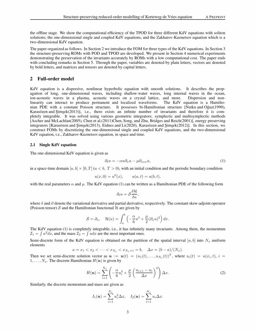
Furthermore, we show the propagation of the relative L2-errors ‖u(x, t) − ue(x, t)‖L2(Ω)/‖ue(x, t)‖L2(Ω) between

the exact solution ue(x, t) and FOM/ROM solutions in Figure 7. The circles indicate that the maximum of the errorsoccur at the final time. In the reduced order modelling framework, the reduced solutions are expected to behavesimilar to the full solutions, since the reduced space is constructed from the FOM. Correspondingly, the errors of thereduced solutions in Figure 7 show similar behavior as the full solution errors. This also indicates that the locationand the shape of the full soliton waves are well-captured by the ROM solutions with increasing number of modes. Thealmost linear error growth rate in time in Figure 7 is characteristic for Hamiltonian preserving and for the geometricintegrators [Hairer et al.(2010)Hairer, Lubich, and Wanner] including Kahan’s method.

20 40 60 80 100 12010

−5

10−4

10−3

10−2

10−1

100

Time

Rel

ativ

e E

rror

FOMROM, n=10ROM, n=15ROM, n=30

Figure 7: Error propagation of relative L2-errors between exact and FOM/ROM solutions.

In Figure 8, the Hamiltonian errors do not show any drift, they are preserved not with a high accuracy as in the singlesoliton example, which might be due to the interaction of the solitons.

13


0 20 40 60 80 100 1200

0.2

0.4

0.6

0.8

1x 10

−6 FOM

Time

H(u

k)−

H(u

0)

0 20 40 60 80 100 120−1

−0.5

0

0.5

1

1.5

2

2.5x 10

−4 ROM

Time

H(u

k r)−

H(u

0 r)


4.3 Coupled KdV equation

Symmetric KdV-KdV equation under periodic boundary conditions possesses solitary pulse solutions decay-ing symmetrically to oscillations of small, constant amplitude [Bona et al.(2007)Bona, Dougalis, and Mitsotakis,Bona et al.(2008)Bona, Dougalis, and Mitsotakis]. The solutions are in the form of traveling waves withmain pulses like the classical solitary waves and dispersive oscillations following the main pulses. Forthe coupled KdV-KdV equation (8), we take the initial conditions as in [Karasozen and Simsek(2012),Bona et al.(2008)Bona, Dougalis, and Mitsotakis]

u(x, 0) = 0 , v(x, 0) = 0.3e−(x+100)2/25.

We set the space-time domain as [−150, 150]× [0, 50], and the mesh sizes are ∆x = 0.1 and ∆t = 0.05. The size ofthe snapshot matrix is Q ∈ R

3000×1000.

In Figure 9 the singular values decay monotonically without reaching a plateau as for the single KdV equation withβ = 10 in Figure 1. The number of modes is determined again by the RIC formula (22) as n = 30 and n = 28 for uand v components, respectively. The reduced and full solutions4 in Figure 10 are visually indistinguishable, and againthe discrete Hamiltonian(9) is preserved accurately by the ROMs in Figure 11.

10 30 50 70 90 110 13010

−15

10−10

10−5

100

n

Nor

mal

ized

sin

gula

r va

lues

uv

Figure 9: Singular values of the snapshot matrices.


14


−150 −100 −50 0 50 100 150−0.2

−0.1

0

0.1

0.2

x

u

FOM−u

−150 −100 −50 0 50 100 150

0

0.05

0.1

0.15

0.2

x

v

FOM−v

−150 −100 −50 0 50 100 150−0.2

−0.1

0

0.1

0.2

x

u

ROM−u

−150 −100 −50 0 50 100 150

0

0.05

0.1

0.15

0.2

x

v

ROM−v

Figure 10: FOM and ROM solutions at T = 50.

0 10 20 30 40 50−4

−3

−2

−1

0

1

2

3

4

5x 10

−16 FOM

Time

H(u

k,vk)−

H(u

0,v0)

0 10 20 30 40 50−4

−2

0

2

4

6

8x 10

−16 ROM

Time

H(u

k r,vk r)−

H(u

0 r,v0 r)


4.4 Zakharov-Kuznetsov equation

We simulate cylindrically symmetric waves of the Zakharov-Kuznetsov equation (11), that are calledas bell-shaped pulses [Chen et al.(2011)Chen, Song, and Zhu, Iwasaki et al.(1990)Iwasaki, Toh, and Kawahara,Nishiyama et al.(2012)Nishiyama, Noi, and Oharu] with α = 6, µ = 1. The initial condition for two pulses is givenby

u(x, y, 0) =2∑

j=1

cj3

10∑

m=1

a2m

(cos

(2marccot

(√cj

2rj

))− 1

),

where c1 and c2 are the velocities of the solitary wave solutions, and ri is defined by r2i = (x − xi)2 + (y −

yi)2, i = 1, 2. The points (xi, yi) are the location of the peak of u. The coefficients a2m are given in

[Nishiyama et al.(2012)Nishiyama, Noi, and Oharu].

Numerical solutions are computed in the rectangular space domain [0, 32]× [0, 32] and in the time interval [0, 5] usinga fine discretization both in space and time, ∆x = ∆y = 0.2286, ∆t = 0.01, to simulate the waves accurately as in

15


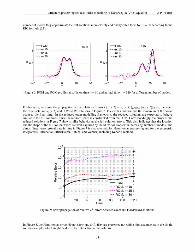
[Chen et al.(2011)Chen, Song, and Zhu, Nishiyama et al.(2012)Nishiyama, Noi, and Oharu]. The snapshot matrix isof size 19600× 500.

The decay of the singular values in Figure 12 shows similar behavior as for the single KdV equations in the Figure 1and in the Figure 9. The number of retained POD modes is n = 50 according to the RIC formula.

0 100 200 300 400 50010

−15

10−10

10−5

100

n

Nor

mal

ized

sin

gula

r va

lues

Figure 12: Singular values of the snapshot matrix.

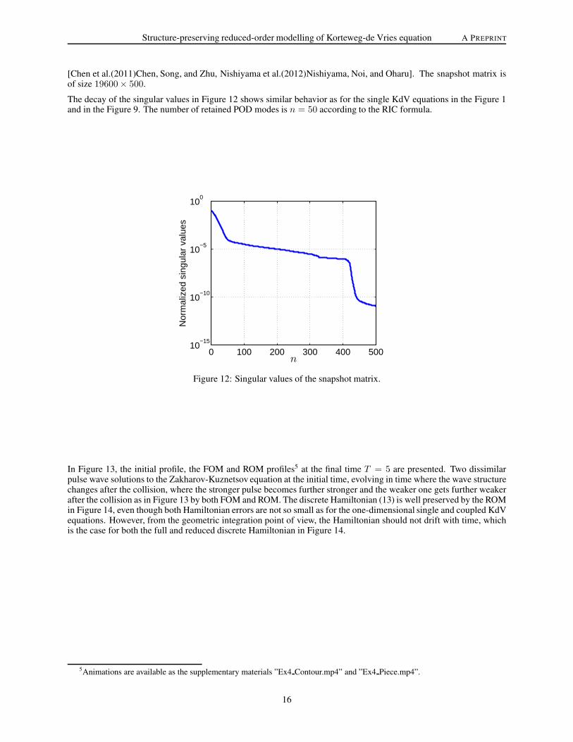
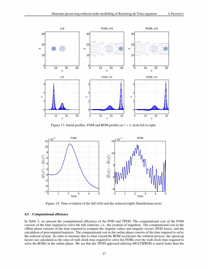
In Figure 13, the initial profile, the FOM and ROM profiles5 at the final time T = 5 are presented. Two dissimilarpulse wave solutions to the Zakharov-Kuznetsov equation at the initial time, evolving in time where the wave structurechanges after the collision, where the stronger pulse becomes further stronger and the weaker one gets further weakerafter the collision as in Figure 13 by both FOM and ROM. The discrete Hamiltonian (13) is well preserved by the ROMin Figure 14, even though both Hamiltonian errors are not so small as for the one-dimensional single and coupled KdVequations. However, from the geometric integration point of view, the Hamiltonian should not drift with time, whichis the case for both the full and reduced discrete Hamiltonian in Figure 14.

5Animations are available as the supplementary materials ”Ex4 Contour.mp4” and ”Ex4 Piece.mp4”.

16


t=0

x

y

0 10 20 300

10

20

30

FOM, t=5

x

y

0 10 20 300

10

20

30

ROM, t=5

x

y

0 10 20 300

10

20

30

0 10 20 30

0

1

2

3

t=0

x

u

0 10 20 30

0

1

2

3

FOM, t=5

x

u

0 10 20 30

0

1

2

3

ROM, t=5

x

u

Figure 13: Initial profiles, FOM and ROM profiles at t = 5, from left to right.

0 1 2 3 4 5−6

−4

−2

0

2

4

6

8

10

12x 10

−3 FOM

Time

H(u

k)−

H(u

0)

0 1 2 3 4 5

−5

0

5

10

15x 10

−3 ROM

Time

H(u

k r)−

H(u

0 r)


4.5 Computational efficiency

In Table 3, we present the computational efficiency of the POD and TPOD. The computational cost of the FOMconsists of the time required to solve the full solutions, i.e., the creation of snapshots. The computational cost in theoffline phase consists of the time required to compute the singular values and singular vectors (POD basis), and thecalculation of precomputed matrices. The computational cost in the online phase consists of the time required to solvethe reduced system. In order to measure that to what extend the ROM accelerates the solution process, the speed-upfactors are calculated as the ratio of wall-clock time required to solve the FOMs over the wall-clock time required tosolve the ROMs in the online phase. We see that the TPOD approach utilizing MULTIPROD is much faster than the

17


POD, where speed-up factors are given in parenthesis in Table 3. The efficiency of the TPOD over the POD is muchpronounced for the KdV equation with one soliton wave and β = 1.5, and for the Zakharov-Kuznetsov equation,because of larger spatial discretization of the FOMs. In addition, for the single KdV equation with one soliton, thecomputational efficiency deteriorates with the increasing values of β and the number of modes.

Table 3: Wall clock times (in seconds) and speed-up factors (in bold parenthesis)

System n FOMPOD TPOD

Offline Online Offline OnlineOne soliton (β = 1.5) 30 178.06 5.28 62.66 (2.8) 5.67 5.55 (32.1)

One soliton (β = 5) 60 185.62 7.49 80.70 (2.3) 8.11 46.30 (4.0)

One soliton (β = 10) 90 188.81 8.25 157.34 (1.2) 9.79 124.40 (1.5)

Two solitons 30 7.26 1.70 2.94 (2.5) 1.71 2.34 (3.1)

Coupled KdV 30, 28 17.85 1.96 2.97 (6.0) 2.01 1.79 ( 9.9)

Zakharov-Kuznetsov equation 50 61.15 3.33 9.25 (6.6) 3.67 0.90 (68.1)

5 Conclusions

We have constructed computationally efficient and accurate ROMs for KdV equations by exploiting the non-canonicalHamiltonian structure. It is difficult to capture the wave dynamics of PDEs like the KdV equation with a few PODmodes. Therefore, in all numerical test problems, the number of the POD modes is relatively large to achieve accuratereduced solutions and to preserve the conserved quantities. Using TPOD and exploiting the quadratic structure of theKdV equations, the online computational time of ROMs is reduced further. In a future study, we plan to extend theresults of this paper to the parametrized problems using the POD/TPOD-greedy approach in time and in parametricspace.

Acknowledgemets: The authors thank for the constructive comments of the referees, which helped much to improvethe paper.

References

[Benner et al.(2017)Benner, Cohen, Ohlberger, and Willcox] P. Benner, A. Cohen, M. Ohlberger, K. Willcox (Eds.),Model reduction and approximation, volume 15 of Computational Science & Engineering, Society for Industrialand Applied Mathematics (SIAM), Philadelphia, PA, 2017. doi:doi:10.1137/1.9781611974829.

[Quarteroni and Rozza(2014)] A. Quarteroni, G. Rozza (Eds.), Reduced order methods for modeling and com-putational reduction, volume 9 of MS&A. Modeling, Simulation and Applications, Springer, Cham, 2014.doi:doi:10.1007/978-3-319-02090-7, selected papers from the workshop “Reduced Basis, POD and ReducedOrder Methods for Model and Computational Reduction: Towards Real-Time Computing and Visualization?”held at Ecole Polytechnique Federale de Lausanne, Lausanne, May 14–16, 2012.

[Hesthaven et al.(2016)Hesthaven, Rozza, and Stamm] J. S. Hesthaven, G. Rozza, B. Stamm, Certified reduced basismethods for parametrized partial differential equations, SpringerBriefs in Mathematics, Springer, Cham; BCAMBasque Center for Applied Mathematics, Bilbao, 2016. doi:doi:10.1007/978-3-319-22470-1, bCAM Springer-Briefs.

[Berkooz et al.(1993)Berkooz, Holmes, and Lumley] G. Berkooz, P. Holmes, J. L. Lumley, The proper orthogonaldecomposition in the analysis of turbulent flows, Annual Review of Fluid Mechanics 25 (1993) 539–575.doi:doi:10.1146/annurev.fl.25.010193.002543.

[Sirovich(1987)] L. Sirovich, Turbulence and the dynamics of coherent structures. III. Dynamics and scaling, Quart.Appl. Math. 45 (1987) 583–590. doi:doi:10.1090/qam/910464.

[Hairer et al.(2016)Hairer, Lubich, and Wanner] E. Hairer, C. Lubich, G. Wanner, Geometric numerical integration:Structure-preserving algorithms for ordinary differential equations, Springer Series in Computational Mathemat-ics, Springer, Heidelberg, 2016. doi:doi:10.1007/978-3-662-05018-7.

[Carlberg et al.(2013)Carlberg, Farhat, Cortial, and Amsallem] K. Carlberg, C. Farhat, J. Cortial, D. Amsallem,The GNAT method for nonlinear model reduction: effective implementation and application to compu-

18

https://doi.org/10.1137/1.9781611974829

https://doi.org/10.1007/978-3-319-02090-7

https://doi.org/10.1007/978-3-319-22470-1

https://doi.org/10.1146/annurev.fl.25.010193.002543

https://doi.org/10.1090/qam/910464

https://doi.org/10.1007/978-3-662-05018-7


tational fluid dynamics and turbulent flows, Journal of Computational Physics 242 (2013) 623 – 647.doi:doi:10.1016/j.jcp.2013.02.028.

[Chaturantabut et al.(2016)Chaturantabut, Beattie, and Gugercin] S. Chaturantabut, C. Beattie, S. Gugercin,Structure-preserving model reduction for nonlinear port-Hamiltonian systems, SIAM Journal on ScientificComputing 38 (2016) B837–B865. doi:doi:10.1137/15M1055085.

[Afkham and Hesthaven(2019)] B. M. Afkham, J. S. Hesthaven, Structure-preserving model-reduction of dissipativeHamiltonian systems, J. Sci. Comput. 81 (2019) 3–21. doi:doi:10.1007/s10915-018-0653-6.

[Afkham and Hesthaven(2017)] B. M. Afkham, J. S. Hesthaven, Structure preserving model reduction of parametricHamiltonian systems, SIAM J. Sci. Comput. 39 (2017) A2616–A2644. doi:doi:10.1137/17M1111991.

[Buchfink et al.(2019)Buchfink, Bhatt, and Haasdonk] P. Buchfink, A. Bhatt, B. Haasdonk, Symplectic modelorder reduction with non-orthonormal bases, Mathematical and Computational Applications 24 (2019).doi:doi:10.3390/mca24020043.

[Hesthaven and Pagliantini(2020)] J. S. Hesthaven, C. Pagliantini, Structure-preserving reduced basis methods forHamiltonian systems with a state-dependent Poisson structure, Mathematics of Computation (2020). URL:http://infoscience.epfl.ch/record/256097.

[Peng and Mohseni(2016)] L. Peng, K. Mohseni, Symplectic model reduction of Hamiltonian systems, SIAM Journalon Scientific Computing 38 (2016) A1–A27. doi:doi:10.1137/140978922.

[Karasozen and Uzunca(2018)] B. Karasozen, M. Uzunca, Energy preserving model order reduction ofthe nonlinear Schrodinger equation, Advances in Computational Mathematics 44 (2018) 1769–1796.doi:doi:10.1007/s10444-018-9593-9.

[Gong et al.(2017)Gong, Wang, and Wang] Y. Gong, Q. Wang, Z. Wang, Structure-preserving Galerkin PODreduced-order modeling of Hamiltonian systems, Computer Methods in Applied Mechanics and Engineering315 (2017) 780 – 798. doi:doi:10.1016/j.cma.2016.11.016.

[Miyatake(2019)] Y. Miyatake, Structure-preserving model reduction for dynamical systems witha first integral, Japan Journal of Industrial and Applied Mathematics 36 (2019) 1021–1037.doi:doi:10.1007/s13160-019-00378-y.

[Hesthaven and Pagliantini(2018)] J. S. Hesthaven, C. Pagliantini, Structure-Preserving Reduced Basis Methods forHamiltonian Systems with a Nonlinear Poisson Structure, Technical Report, EPFL scientific publications, 2018.URL: http://infoscience.epfl.ch/record/256097.

[Gerbeau and Lombardi(2014)] J.-F. Gerbeau, D. Lombardi, Approximated Lax pairs for the reduced order in-tegration of nonlinear evolution equations, Journal of Computational Physics 265 (2014) 246 – 269.doi:doi:10.1016/j.jcp.2014.01.047.

[Ehrlacher et al.(2020)Ehrlacher, Lombardi, Mula, and Vialard] V. Ehrlacher, D. Lombardi, O. Mula, F. X. Vialard,Nonlinear model reduction on metric spaces. application to one-dimensional conservative PDEs in Wassersteinspaces, ESAIM: Mathematical Modelling and Numerical Analysis (2020). doi:doi:10.1051/m2an/2020013.

[Barrault et al.(2004)Barrault, Maday, Nguyen, and Patera] M. Barrault, Y. Maday, N. C. Nguyen, A. T. Patera, An’empirical interpolation’ method: application to efficient reduced-basis discretization of partial differential equa-tions, C. R. Math. Acad. Sci. Paris 339 (2004) 667–672. doi:doi:10.1016/j.crma.2004.08.006.

[Chaturantabut and Sorensen(2010)] S. Chaturantabut, D. C. Sorensen, Nonlinear model reduction via discrete em-pirical interpolation, SIAM Journal on Scientific Computing 32 (2010) 2737–2764. doi:doi:10.1137/090766498.

[Celledoni et al.(2012)Celledoni, Grimm, McLachlan, McLaren, O’Neale, Owren, and Quispel] E. Celledoni,V. Grimm, R. I. McLachlan, D. I. McLaren, D. O’Neale, B. Owren, G. R. W. Quispel, Preserving energy resp.dissipation in numerical pdes using the ”Average Vector Field” method, Journal of Computational Physics 231(2012) 6770 – 6789. doi:doi:10.1016/j.jcp.2012.06.022.

[Kahan and Li(1997)] W. Kahan, R.-C. Li, Unconventional schemes for a class of ordinary differential equationswith applications to the Korteweg-de Vries equation, Journal of Computational Physics 134 (1997) 316 – 331.doi:doi:10.1006/jcph.1997.5710.

[Celledoni et al.(2013)Celledoni, McLachlan, Owren, and Quispel] E. Celledoni, R. I. McLachlan, B. Owren,G. R. W. Quispel, Geometric properties of Kahan’s method, Journal of Physics A: Mathematical and Theo-retical 46 (2013) 025201. doi:doi:10.1088/1751-8113/46/2/025201.

[Celledoni et al.(2015)Celledoni, McLachlan, McLaren, Owren, and Quispel] E. Celledoni, R. I. McLachlan, D. I.McLaren, B. Owren, G. R. W. Quispel, Discretization of polynomial vector fields by polarization, Pro-ceedings of the Royal Society of London A: Mathematical, Physical and Engineering Sciences 471 (2015).doi:doi:10.1098/rspa.2015.0390.

19

https://doi.org/10.1016/j.jcp.2013.02.028

https://doi.org/10.1137/15M1055085

https://doi.org/10.1007/s10915-018-0653-6

https://doi.org/10.1137/17M1111991

https://doi.org/10.3390/mca24020043

http://infoscience.epfl.ch/record/256097

https://doi.org/10.1137/140978922

https://doi.org/10.1007/s10444-018-9593-9

https://doi.org/10.1016/j.cma.2016.11.016

https://doi.org/10.1007/s13160-019-00378-y

http://infoscience.epfl.ch/record/256097


https://doi.org/10.1051/m2an/2020013

https://doi.org/10.1016/j.crma.2004.08.006

https://doi.org/10.1137/090766498


https://doi.org/10.1006/jcph.1997.5710

https://doi.org/10.1088/1751-8113/46/2/025201

https://doi.org/10.1098/rspa.2015.0390


[Benner et al.(2018)Benner, Goyal, and Gugercin] P. Benner, P. Goyal, S. Gugercin, H2-quasi-optimal model orderreduction for quadratic-bilinear control systems, SIAM Journal on Matrix Analysis and Applications 39 (2018)983–1032. doi:doi:10.1137/16M1098280.

[Benner and Breiten(2015)] P. Benner, T. Breiten, Two-sided projection methods for nonlinear model order reduction,SIAM Journal on Scientific Computing 37 (2015) B239–B260. doi:doi:10.1137/14097255X.

[Kramer and Willcox(2019)] B. Kramer, K. E. Willcox, Nonlinear model order reduction via lifting transformationsand proper orthogonal decomposition, AIAA Journal 57 (2019) 2297–2307. doi:doi:10.2514/1.J057791.

[Benner and Goyal(2021)] P. Benner, P. Goyal, Interpolation-based model order reduction for polynomial systems,SIAM Journal on Scientific Computing 43 (2021) A84–A108. doi:doi:10.1137/19M1259171.

[Leva(2008)] P. D. Leva, MULTIPROD TOOLBOX, multiple matrix multiplications, with array expansion enabled,Technical Report, University of Rome Foro Italico, Rome, 2008.

[Nutku and Oguz(1990)] Y. Nutku, O. Oguz, Bi-Hamiltonian structure of a pair of coupled KdV equations, NuovoCimento B (11) 105 (1990). doi:doi:10.1007/BF02742693.

[Karasozen and Simsek(2013)] B. Karasozen, G. Simsek, Energy preserving integration of bi-Hamiltonian partialdifferential equations, Appl. Math. Lett. 26 (2013) 1125–1133. doi:doi:10.1016/j.aml.2013.06.005.

[Ascher and McLachlan(2005)] U. M. Ascher, R. I. McLachlan, On symplectic and multisymplectic schemes for theKdV equation, Journal of Scientific Computing 25 (2005) 83–104. doi:doi:10.1007/s10915-004-4634-6.

[Chen et al.(2011)Chen, Song, and Zhu] Y. Chen, S. Song, H. Zhu, The multi-symplectic Fourier pseudospectralmethod for solving two-dimensional Hamiltonian PDEs, Journal of Computational and Applied Mathematics236 (2011) 1354 – 1369. doi:doi:10.1016/j.cam.2011.08.023.

[Bridges and Reich(2001)] T. J. Bridges, S. Reich, Multi-symplectic spectral discretizations for the Zakharov-Kuznetsov and shallow water equations, Physica D: Nonlinear Phenomena 152-153 (2001) 491 – 504.doi:doi:10.1016/S0167-2789(01)00188-9.

[Eidnes and Li(2020)] S. Eidnes, L. Li, Linearly implicit local and global energy-preserving methods forPDEs with a cubic Hamiltonian, SIAM Journal on Scientific Computing 42 (2020) A2865–A2888.doi:doi:10.1137/19M1272688.

[Karasozen and Simsek(2012)] B. Karasozen, G. Simsek, Energy preserving integra-tion of KdV-KdV systems, TWMS J. Appl. Eng. Math. 2 (2012) 219–227. URL:http://jaem.isikun.edu.tr/web/images/articles/vol.2.no.2/08.pdf.

[Sanz-Serna(1994)] J. Sanz-Serna, An unconventional symplectic integrator of W. Kahan, Applied Numerical Math-ematics 16 (1994) 245 – 250. doi:doi:10.1016/0168-9274(94)00030-1.

[Matsuo and Furihata(2001)] T. Matsuo, D. Furihata, Dissipative or conservative finite-difference schemes forcomplex-valued nonlinear partial differential equations, Journal of Computational Physics 171 (2001) 425 –447. doi:doi:10.1006/jcph.2001.6775.

[Dahlby and Owren(2011)] M. Dahlby, B. Owren, A general framework for deriving integral preserving numericalmethods for PDEs, SIAM Journal on Scientific Computing 33 (2011) 2318–2340. doi:doi:10.1137/100810174.

[Eidnes et al.(2019)Eidnes, Li, and Sato] S. Eidnes, L. Li, S. Sato, Linearly implicit structure-preservingschemes for Hamiltonian systems, Journal of Computational and Applied Mathematics (2019) 112489.doi:doi:10.1016/j.cam.2019.112489.

[Hardin(1973)] R. H. Hardin, Application of the split-step fourier method to the numerical solution of nonlinear andvariable coefficient wave equations, Siam Review 15 (1973) 423.

[Bona et al.(2007)Bona, Dougalis, and Mitsotakis] J. Bona, V. Dougalis, D. Mitsotakis, Numerical solution of KdV-KdV systems of Boussinesq equations: I. the numerical scheme and generalized solitary waves, Mathematicsand Computers in Simulation 74 (2007) 214 – 228. doi:doi:10.1016/j.matcom.2006.10.004.

[Iwasaki et al.(1990)Iwasaki, Toh, and Kawahara] H. Iwasaki, S. Toh, T. Kawahara, Cylindrical quasi-solitonsof the Zakharov-Kuznetsov equation, Physica D: Nonlinear Phenomena 43 (1990) 293 – 303.doi:doi:10.1016/0167-2789(90)90138-F.

[Nishiyama et al.(2012)Nishiyama, Noi, and Oharu] H. Nishiyama, T. Noi, S. Oharu, Conservative finite differenceschemes for the generalized Zakharov-Kuznetsov equations, Journal of Computational and Applied Mathematics236 (2012) 2998 – 3006. doi:doi:10.1016/j.cam.2011.04.010.

[Zakharov and Kuznetsov(1974)] V. Zakharov, E. Kuznetsov, Three-dimensional solitons, Soviet Physics JETP 29(1974) 594–597.

20

https://doi.org/10.1137/16M1098280

https://doi.org/10.1137/14097255X

https://doi.org/10.2514/1.J057791

https://doi.org/10.1137/19M1259171

https://doi.org/10.1007/BF02742693

https://doi.org/10.1016/j.aml.2013.06.005

https://doi.org/10.1007/s10915-004-4634-6

https://doi.org/10.1016/j.cam.2011.08.023

https://doi.org/10.1016/S0167-2789(01)00188-9

https://doi.org/10.1137/19M1272688

http://jaem.isikun.edu.tr/web/images/articles/vol.2.no.2/08.pdf

https://doi.org/10.1016/0168-9274(94)00030-1

https://doi.org/10.1006/jcph.2001.6775

https://doi.org/10.1137/100810174

https://doi.org/10.1016/j.cam.2019.112489

https://doi.org/10.1016/j.matcom.2006.10.004

https://doi.org/10.1016/0167-2789(90)90138-F



[Xu and Shu(2005)] Y. Xu, C.-W. Shu, Local discontinuous Galerkin methods for two classes of two-dimensional nonlinear wave equations, Physica D: Nonlinear Phenomena 208 (2005) 21 – 58.doi:doi:10.1016/j.physd.2005.06.007.

[Sanderse(2020)] B. Sanderse, Non-linearly stable reduced-order models for incompressible flow withenergy-conserving finite volume methods, Journal of Computational Physics 421 (2020) 109736.doi:doi:https://doi.org/10.1016/j.jcp.2020.109736.

[Reis and Stykel(2007)] T. Reis, T. Stykel, Stability analysis and model order reduction of coupled systems, Math.Comput. Model. Dyn. Syst. 13 (2007) 413–436. doi:doi:10.1080/13873950701189071.

[Benner et al.(2020)Benner, Goyal, Kramer, Peherstorfer, and Willcox] P. Benner, P. Goyal, B. Kramer, B. Pe-herstorfer, K. Willcox, Operator inference for non-intrusive model reduction of systems with non-polynomial nonlinear terms, Computer Methods in Applied Mechanics and Engineering 372 (2020) 113433.doi:doi:10.1016/j.cma.2020.113433.

[Benner et al.(2015)Benner, Gugercin, and Willcox] P. Benner, S. Gugercin, K. Willcox, A survey of projection-based model reduction methods for parametric dynamical systems, SIAM Review 57 (2015) 483–531.doi:doi:10.1137/130932715.

[Stefanescu et al.(2014)Stefanescu, Sandu, and Navon] R. Stefanescu, A. Sandu, I. M. Navon, Comparison of PODreduced order strategies for the nonlinear 2D shallow water equations, International Journal for NumericalMethods in Fluids 76 (2014) 497–521. doi:doi:10.1002/fld.3946.

[Mahoney and Drineas(2009)] M. W. Mahoney, P. Drineas, CUR matrix decompositions for improved data analysis,Proceedings of the National Academy of Sciences 106 (2009) 697–702. doi:doi:10.1073/pnas.0803205106.

[Karasozen et al.(2021)Karasozen, Yıldız, and Uzunca] B. Karasozen, S. Yıldız, M. Uzunca, Structure preservingmodel order reduction of shallow water equations, Mathematical Methods in the Applied Sciences 44 (2021)476–492. doi:doi:10.1002/mma.6751.

[Halko et al.(2011)Halko, Martinsson, and Tropp] N. Halko, P. G. Martinsson, J. A. Tropp, Finding structure withrandomness: Probabilistic algorithms for constructing approximate matrix decompositions, SIAM Review 53(2011) 217–288. doi:doi:10.1137/090771806.

[Ohlberger and Rave(2016)] M. Ohlberger, S. Rave, Reduced basis methods: Success, limita-tions and future challenges, Proceedings of the Conference Algoritmy (2016) 1–12. URL:http://www.iam.fmph.uniba.sk/amuc/ojs/index.php/algoritmy/article/view/389.

[Brugnano et al.(2019)Brugnano, Gurioli, and Sun] L. Brugnano, G. Gurioli, Y. Sun, Energy-conserving Hamiltonianboundary value methods for the numerical solution of the Korteweg-de Vries equation, Journal of Computationaland Applied Mathematics 351 (2019) 117 – 135. doi:doi:10.1016/j.cam.2018.10.014.

[Bo et al.(2020)Bo, Wang, and Cai] Y. Bo, Y. Wang, W. Cai, Arbitrary high-order linearly implicit energy-preservingalgorithms for Hamiltonian PDEs, 2020. arXiv:2011.08375.

[Liu and Yi(2016)] H. Liu, N. Yi, A Hamiltonian preserving discontinuous Galerkin method for the gen-eralized Korteweg-de Vries equation, Journal of Computational Physics 321 (2016) 776 – 796.doi:doi:10.1016/j.jcp.2016.06.010.

[Hairer et al.(2010)Hairer, Lubich, and Wanner] E. Hairer, C. Lubich, G. Wanner, Geometric numerical integration,volume 31 of Springer Series in Computational Mathematics, Springer, Heidelberg, 2010. Structure-preservingalgorithms for ordinary differential equations, Reprint of the second (2006) edition.

[Bona et al.(2008)Bona, Dougalis, and Mitsotakis] J. L. Bona, V. A. Dougalis, D. E. Mitsotakis, Numerical solutionof Boussinesq systems of KdV-KdV type. II. Evolution of radiating solitary waves, Nonlinearity 21 (2008)2825–2848. doi:doi:10.1088/0951-7715/21/12/006.

21

https://doi.org/10.1016/j.physd.2005.06.007

https://doi.org/https://doi.org/10.1016/j.jcp.2020.109736

https://doi.org/10.1080/13873950701189071

https://doi.org/10.1016/j.cma.2020.113433

https://doi.org/10.1137/130932715

https://doi.org/10.1002/fld.3946

https://doi.org/10.1073/pnas.0803205106

https://doi.org/10.1002/mma.6751

https://doi.org/10.1137/090771806

http://www.iam.fmph.uniba.sk/amuc/ojs/index.php/algoritmy/article/view/389


http://arxiv.org/abs/2011.08375


https://doi.org/10.1088/0951-7715/21/12/006

structure-preserving reduced-order modelling of korteweg-de ...

Documents

Transcript of structure-preserving reduced-order modelling of korteweg-de ...