A partial differential equation formulation of Vickrey’s bottleneck model, part II: Numerical...

Transportation Research Part B 49 (2013) 75–93

Contents lists available at SciVerse ScienceDirect

Transportation Research Part B

journal homepage: www.elsevier .com/ locate/ t rb

A partial differential equation formulation of Vickrey’sbottleneck model, part II: Numerical analysis and computation q

0191-2615/$ - see front matter � 2012 Elsevier Ltd. All rights reserved.http://dx.doi.org/10.1016/j.trb.2012.10.004

q This work was partially supported by NSF through Grant EFRI-1024707, ‘‘A theory of complex transportation network design’’.⇑ Corresponding author. Tel.: +1 814 863 2445.

E-mail addresses: [email protected] (K. Han), [email protected] (T.L. Friesz), [email protected] (T. Yao).

Ke Han a, Terry L. Friesz b,⇑, Tao Yao b

a Department of Mathematics, Pennsylvania State University, PA 16802, USAb Department of Industrial and Manufacturing Engineering, Pennsylvania State University, PA 16802, USA

a r t i c l e i n f o

Keywords:The Vickrey model
Discrete-time solutionConvergenceSystem optimal dynamic traffic assignmentMixed integer linear program
a b s t r a c t

The Vickrey model, originally introduced in Vickrey (1969), is one of the most widely usedlink-based models in the current literature in dynamic traffic assignment (DTA). One popularformulation of this model is an ordinary differential equation (ODE) that is discontinuouswith respect to its state variable. As explained in Ban et al. (2011) and Han et al. (2013),such an irregularity induces difficulties in both continuous-time analysis and discrete-timecomputation. In Han et al. (2013), the authors proposed a reformulation of the Vickreymodel as a partial differential equation (PDE) and derived a closed-form solution to theaforementioned ODE. This reformulation enables us to rigorously prove analytical proper-ties of the Vickrey model and related DTA models.

In this paper, we present the second of a two-part exploration regarding the PDE formu-lation of the Vickrey model. As proposed by Han et al. (2013), we continue research on thegeneralized Vickrey model (GVM) in a discrete-time framework and in the context of DTA bypresenting a highly computable solution methodology. Our new computational scheme forthe GVM is based on the closed-form solution mentioned above. Unlike finite-differencediscretization schemes which could yield non-physical solutions (Ban et al., 2011), the pro-posed numerical scheme guarantees non-negativity of the queue size and the exit flow aswell as first-in-first-out (FIFO). Numerical errors and convergence of the computed solu-tions are investigated in full mathematical rigor. As an application of the GVM, a class ofnetwork system optimal dynamic traffic assignment (SO-DTA) problems is analyzed. Weshow existence of a continuous-time optimal solution and propose a discrete-time mixedinteger linear program (MILP) as an approximation to the original SO-DTA. We also provideconvergence results for the proposed MILP approximation.

� 2012 Elsevier Ltd. All rights reserved.

1. Introduction

1.1. Existing work

The Vickrey model, initially proposed in Vickrey (1969), has been widely studied in DTA problems; as examples see Dri-ssi-Katouni and Hameda-Benchekroun (1992), Heydecker and Addison (1996), Kuwahara and Akamatsu (1997), and Li et al.(2000). The model is based on two main assumptions: (i) vehicles enter a link and travel with free-flow speed until theyreach the exit, which is a bottleneck with capacity M; (ii) if the flow arriving at the bottleneck exceeds the capacity, a queue

http://crossmark.dyndns.org/dialog/?doi=10.1016/j.trb.2012.10.004&domain=pdf

http://dx.doi.org/10.1016/j.trb.2012.10.004

mailto:[email protected]




http://www.sciencedirect.com/science/journal/01912615

http://www.elsevier.com/locate/trb

76 K. Han et al. / Transportation Research Part B 49 (2013) 75–93

with no physical length will form. For this reason, the Vickrey model is sometimes referred to as the point queue model(PQM).1 The primary mathematical formulation of the Vickrey model is an ordinary differential equation with a discontinuousright hand side (Kuwahara and Akamatsu, 1997; Nie and Zhang, 2005). Such an ODE does not enjoy a wide range of provablemathematical properties. The reader is referred to Filippov (1988) and Stewart (1990) for some case-specific discussions onODEs with discontinuities. Due to the discontinuous right hand side, the Vickrey ODE does not admit any classical solution,i.e. solution that is locally continuously differentiable and satisfies the ODE everywhere.

In Han et al. (2013), a partial differential equation reformulation of the Vickrey model was proposed. In particular,with a virtual spatial dimension x, the link dynamic was described by a scalar conservation law with an x-dependentflux function. Since such an x-dependence is discontinuous, the solution to the scalar conservation law exists only in adistributional sense. In other words, the local density function could contain the dirac-delta, which is the mathematicalabstraction of the well-known notion of ‘‘point queue’’. In order to solve such a non-classical PDE, the authors invokedan equivalent Hamilton–Jacobi equation and employed a variational method known as the Lax–Hopf formula. The Lax–Hopf formula was initially introduced by Lax (1957, 1973) for scalar conservation laws, then extended by Aubin et al.(2008), Bardi and Capuzzo Dolcetta (1997), and Floch (1988) and applied to traffic flow theory in Claudel and Bayen(2010), Daganzo (2005), and Friesz et al. (2013). The Lax–Hopf formula provides a new characterization of solutionsto the scalar conservation law and to the Hamilton–Jacobi equation. It was derived from the characteristics equationsassociated with the Hamilton–Jacobi PDE, which arose from the calculus of variations and classical mechanics. We referthe reader to Evans (2010) for a comprehensive discussion. Han et al. (2013) adapted the Lax–Hopf formula to an H-Jequation with x-dependent Hamiltonian, and derived an explicit solution to the equation. Based on such a solution, theauthors provided a closed-form solution to Vickrey’s ODE with a discontinuous right hand side.

The closed-form solution of the Vickrey ODE leads to an extension of the model, which we call the generalized Vick-rey model (GVM). The GVM is based on traffic quantities that describe the volume, such as the cumulative enteringand exiting vehicle counts and the queue size. All these quantities, plus the link traversal time function, can be ex-pressed explicitly once the cumulative entering vehicle count Uð�Þ : ½0; T� ! Rþ is given. Furthermore, the GVM relieson a weakened regularity assumption on U(�): the cumulative entering vehicle count U(�) can have jump discontinuities.Such an assumption is more general than that made in the Vickrey model since the latter requires the link enteringflow to be Lebesgue integrable, which implies that U(�) is absolutely continuous. Such a relaxed regularity conditionis used for convenience in analysis of DTA models. As we explain later in this paper, existence of solutions to anSO-DTA problem relies on the generalized assumption on U(�). In Bressan and Han (2011), a class of dynamic user equi-librium models was investigated. Solutions of these models exist only when the cumulative departure curves areallowed to contain jump discontinuities. Such regularity assumptions, although not realistic in real-world traffic, arecrucial for analyzing DTA problems and for studying further mathematical properties of the network performancemodels that are based on the Vickrey model.

1.2. Findings

This paper is concerned with the computation and application of the GVM. In particular, we aim to fix the numer-ical problems commonly identified in finite-difference schemes for the Vickrey ODE: the resulting solutions may con-tain negative queue size and negative flow (Ban et al., 2011). In this paper, we propose a new computational methodbased on the GVM. The resulting discrete solution is shown to provide physical realism, such as non-negativity of thequeue size and flow, as well as the first-in-first-out principle. In contrast to many finite-difference schemes, the pro-posed algorithm imposes no constraints on the time step size or the uniformity of the time grid. The closed-form rep-resentations of key variables provided by the GVM enable us to investigate the numerical error of the attained discretesolution, and to establish convergence for the proposed approximation. As stated and proved in Theorem 3.8, theapproximate solution converges uniformly to the exact solution of the GVM when the time step size goes to zero.Such a convergence result provides a theoretical guarantee of the numerical efficacy of the proposed computationalmethod.

In this paper, we present an application of the GVM to system optimal dynamic traffic assignment (SO-DTA) problems.The SO-DTA problems have been primarily studied using mathematical programming (Carey, 1987; Merchant and Nemha-user, 1978a; Merchant and Nemhauser, 1978b; Ziliaskopoulos, 2000) and optimal control (Friesz et al., 1989; Ran and Shi-mazaki, 1989; Wie et al., 1990). Our proposed methodology for studying SO-DTA belongs to the first category. We presentboth continuous-time and discrete-time formulations of the SO-DTA problems. Existence is established for the continuous-time (infinite-dimensional) math program, using the generalized Vickrey model. Such a result is non-trivial and difficult toestablish without the reformulation of the Vickrey model. In order to compute the system optimal solution, we propose adiscrete-time mixed integer linear program as an adequate approximation to the original SO-DTA. The MILP can be effi-ciently solved with standard commercial solvers, such as CPLEX. Convergence results for the proposed MILP approximationare established as well, in Section 4.4.

1 The authors of this paper are reluctant to use the name PQM since it was first used by Daganzo (1994) to describe the link delay model (LDM), initiallyproposed by Friesz et al. (1993).

K. Han et al. / Transportation Research Part B 49 (2013) 75–93 77

1.3. Organization

The rest of this article is organized as follows. In Section 2, we review the main results from Han et al. (2013). InSection 3, we propose a method for numerically computing the solution to the generalized Vickrey model. Errorestimates and convergence results are provided as well. Moreover, we show results regarding the physical realismof the discrete solutions. In Section 4, we consider a network SO-DTA problem expressed as an infinite-dimensionalmathematical program using the GVM. Existence of a continuous-time optimal solution is shown. A mixed integerlinear program (MILP) is proposed to approximate the SO-DTA problem. Convergence results for the proposedMILP approximation are provided. In Section 5, a few numerical solutions to the GVM and to the MILP arepresented.

2. The generalized Vickrey model

The Vickrey model (Vickrey, 1969) can be briefly described as follows. It assumes that vehicles entering a link travel at afree-flow speed before they reach the exit which is a bottleneck. When the flow arriving at the bottleneck exceeds the capac-ity, a queue with no physical length will form. We denote the free flow travel time by t0 and the bottleneck capacity by M. Inaddition, we introduce the following notations.

uðtÞ : link entering flow at time t

qðtÞ : queue size at time t

wðtÞ : link exiting flow at time t

WðtÞ : cumulative link exiting vehicle count by time t

kðtÞ : link traversal time of driver who enters the link at time t

The Vickrey model can be mathematically expressed by an ordinary differential equation of the following form

dqðtÞdt¼ uðt � t0Þ �

minfuðt � t0Þ;Mg if qðtÞ ¼ 0M if qðtÞ > 0

�ð2:1Þ

Notice that ODE (2.1) has a right hand side that is discontinuous w.r.t. the unknown q(�). Such an irregularity is prob-lematic in both theoretical analysis and numerical computation, see Ban et al. (2011) and Han et al. (2013) for somediscussions. In Han et al. (2013), ODE (2.1) was reformulated as a scalar conservation law, based on which an explicitsolution to the ODE was provided. The explicit solution representation led to the generalized Vickrey model (GVM),which we present below.

We consider a time horizon of [0, T] for any T > 0. Let us introduce the cumulative entering vehicle count Uð�Þ : ½0; T� ! Rþ,which is left-continuous and non-decreasing. Notice that in the GVM, U(�) is not necessarily absolutely continuous, whichwould be the case if u(�) were Lebesgue integrable and U(�) is expressed as the integral of u(�)

UðtÞ ¼Z t

0uðsÞds

Therefore, the GVM is more general than the original Vickrey model in that weaker regularity assumptions on U(�) and u(�)are made.

Definition 2.1 (The Generalized Vickrey Model). Given the entering vehicle count Uð�Þ; ½0; T� ! Rþ, which is left-continuousand non-decreasing, the GVM is defined in terms of q(�), W(�) and k(�) given by (2.2), (2.3) and (2.4), respectively.

qðtÞ ¼ Uðt � t0Þ �Mðt � t0Þ � min06s6t�t0

fUðsÞ �Msg t 2 ½t0; T þ t0� ð2:2Þ

WðtÞ ¼ min06s6t�t0

fUðsÞ �Msg þMðt � t0Þ t 2 ½t0; T þ t0� ð2:3Þ

kðtÞ ¼ qðt þ t0Þ=M þ t0 t 2 ½0; T� ð2:4Þ
In the generalized Vickrey model, once the inflow profile U(�) is given, all the other variables of interest are presented in
closed-form. As we demonstrate in the rest of this paper, the closed-form solutions allow for rigorous mathematical analysisand efficient computation. In addition, the GVM can treat discontinuous U(�), which is a desirable feature when DTA prob-lems are analyzed. In the next section, we propose both continuous-time and discrete-time computational schemes for theGVM, based on formulae (2.2)–(2.4). Results regarding solution properties and error estimates are established as well.

3. Computational method

We start with the continuous-time formulae for computing the right hand sides of (2.2)–(2.4), based on an additionalassumption that the cumulative entering vehicle count is piecewise affine (PWA).


3.1. Continuous-time formulae

Assume that bUð�Þ is left-continuous, non-decreasing and piecewise affine. Let fnigmi¼1 � ½0; T� be the set of break points ofbUð�Þ. By convention, we set n1 = 0. For each t 2 [t0, T + t0], define the finite set Xt ¼

: {ni: ni 6 t � t0} [ {t � t0}. Then the righthand sides of (2.2)–(2.4) can be computed explicitly in continuous-time.

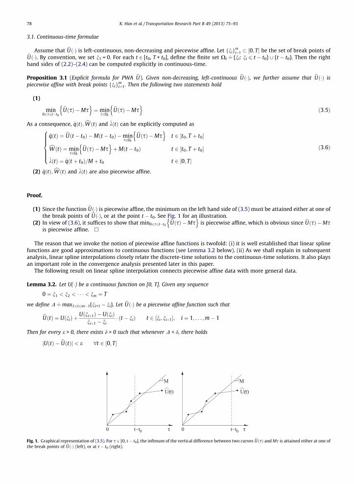
Proposition 3.1 (Explicit formula for PWA bU). Given non-decreasing, left-continuous bUð�Þ, we further assume that bUð�Þ ispiecewise affine with break points fnigm

i¼1. Then the following two statements hold

(1)

Fig. 1.the bre

min06s6t�t0

bUðsÞ �Msn o

¼ mins2Xt

bUðsÞ �Msn o

ð3:5Þ

As a consequence, qðtÞ;cW ðtÞ and kðtÞ can be explicitly computed as

qðtÞ ¼ bUðt � t0Þ �Mðt � t0Þ �mins2Xt

bUðsÞ �Msn o

t 2 ½t0; T þ t0�

cW ðtÞ ¼ mins2Xt

bUðsÞ �Msn o

þMðt � t0Þ t 2 ½t0; T þ t0�

kðtÞ ¼ qðt þ t0Þ=M þ t0 t 2 ½0; T�

8>>>><>>>>: ð3:6Þ

(2) qðtÞ;cW ðtÞ and kðtÞ are also piecewise affine.

Proof.

(1) Since the function bUð�Þ is piecewise affine, the minimum on the left hand side of (3.5) must be attained either at one ofthe break points of bUð�Þ, or at the point t � t0. See Fig. 1 for an illustration.

(2) In view of (3.6), it suffices to show that min06s6t�t0bUðsÞ �Ms

n ois piecewise affine, which is obvious since bUðsÞ �Ms

is piecewise affine. h

The reason that we invoke the notion of piecewise affine functions is twofold: (i) it is well established that linear splinefunctions are good approximations to continuous functions (see Lemma 3.2 below). (ii) As we shall explain in subsequentanalysis, linear spline interpolations closely relate the discrete-time solutions to the continuous-time solutions. It also playsan important role in the convergence analysis presented later in this paper.

The following result on linear spline interpolation connects piecewise affine data with more general data.

Lemma 3.2. Let U(�) be a continuous function on [0, T]. Given any sequence

0 ¼ n1 < n2 < � � � < nm ¼ T

we define D ¼: max16i6m�1{ni+1 � ni}. Let bUð�Þ be a piecewise affine function such that

bUðtÞ ¼ UðniÞ þUðniþ1Þ � UðniÞ

niþ1 � ni� ðt � niÞ t 2 ½ni; niþ1�; i ¼ 1; . . . ;m� 1

Then for every e > 0, there exists d > 0 such that whenever D < d, there holds

jUðtÞ � bUðtÞj < e 8t 2 ½0; T�

Graphical representation of (3.5). For s 2 [0, t � t0], the infimum of the vertical difference between two curves bUðsÞ and Ms is attained either at one ofak points of bUð�Þ (left), or at t � t0 (right).


Lemma 3.2 is a well-known result so its proof is omitted from the paper. We denote C0[0, T] to be the space of continuousfunctions on [0, T] equipped with the supremum norm

kfkC0 ½0;T�¼: max

06t6Tjf ðtÞj f 2 C0½0; T�

Then Lemma 3.2 states that any C0 function can be approximated uniformly by linear spline functions. In other words, the setof continuous piecewise affine functions is dense in C0[0, T].

3.2. Discrete-time solution

Let us consider discrete-time solutions of the GVM. We introduce a uniform time grid with step size h

0 ¼ t1 < t2 < � � � < tN ¼ T

As usual, we consider the left-continuous and non-decreasing inflow profile U(�). For brevity of notations, we let

Ui ¼: UðtiÞ; qi ¼

: qðtiÞ; Wi ¼: WðtiÞ; ki ¼

:kðtiÞ; l ¼: dt0

he ð3:7Þ

The operator d�e rounds its argument to the nearest integer from above. Notice that the Vickrey model involves a backward timeshift by t0, which represents the free-flow phase. If t0 is not a multiple of the time step h, we consider the approximation using d�e.

In the next theorem, we provide formulae for discrete-time solutions of the GVM as well as sharp estimates of the errorwhen t0 is not a multiple of h.

Theorem 3.3 (Discrete-time solution). Given constants t0, M, discrete values fUigNi¼1 and initial data q1 = 0, the discrete-time

solutions Wi and qi are given by

Wi ¼0 1 6 i 6 lmin

16j6i�lfUj �Mtjg þMðti � t0Þ l < i 6 N þ l

(ð3:8Þ

qi ¼ Ui�l �Mti�l � min16j6i�l

fUj �Mtjg 1þ l 6 i 6 N þ l ð3:9Þ

In addition, we let bUð�Þ be a continuous-time PWA function with break points fti;UigNi¼1, and let cW ð�Þ be the corresponding solution

satisfying (3.6). Then the above discrete-time solutions satisfy

0 6 qi 1þ l 6 i 6 N þ l; ð3:10Þ0 6Wi 6Wiþ1 l < i 6 N þ l� 1 ð3:11Þ

0 6Wi � cW ðtiÞ 6 dt0

he � t0

h

� �hM; l < i 6 N þ l ð3:12Þ

In particular, if t0h is integer, the discrete solutions (3.8) and (3.9) become exact.

In the statement of Theorem 3.3, we agree, without causing any confusion, that ti ¼: T + (i � N)h when i > N.

Remark 3.4. Notice that for i 6 l, Wi is zero since it takes a car at least l time intervals to traverse a link. Inequalities (3.10)and (3.11) imply non-negativity of the queue size and the exit flow. Inequality (3.12) provides an upper bound on the error inthe case where the free-flow time t0 is not a multiple of the time step h.

Remark 3.5. We note that the proposed numerical method is unconditionally stable since it imposes no requirement on the timestep size or uniformity of the time grid. (3.12) implies that the error in the solution grows at most linearly with the time step.

Proof. (3.10) follows immediately from (3.9). For (3.11), notice that the quantity

min16j6i�l

fUj �Mtjg � min16j6iþ1�l

fUj �Mtjg

is equal to either 0 or min16j6i�l{Uj �Mtj} � (Ui+1�l �Mti+1�l). In the latter case

min16j6i�l


fUj �Mtjg 6 Ui�l �Mti�l � ðUiþ1�l �Mtiþ1�lÞ 6 Mh

Thus

Wi �Wiþ1 ¼ min16j6i�l


fUj �Mtjg �Mh 6 0

This shows monotonicity. To show non-negativity, it suffices to check that Wl+1 P 0.


For error estimate (3.12), recall l ¼ dt0he. It then follows from (3.6) and the definition of Xt that

cW ðtiÞ ¼mins2Xti

bUðsÞ �Msn o

þ ðti � t0ÞM ¼min min16j6i�l

bUðtjÞ �Mtj

n o; bUðti � t0Þ �Mðti � t0Þ

� �þ ðti � t0ÞM 6Wi

The above strict inequality holds if and only if
bUðti � t0Þ �Mðti � t0Þ < min16j6i�l
bUðtjÞ �Mtj

n o
In this case, we have the estimate
Wi � cW ðtiÞ ¼ min16j6i�l

bUðtjÞ �Mtj

n o� bUðti � t0Þ þMðti � t0Þ 6 bUðti�lÞ �Mti�l � bUðti � t0Þ þMðti � t0Þ

6 Mðti � t0 � ti�lÞ ¼ Mðti � t0 � ti þ lhÞ ¼ Mh l� t0

h

� �
This verifies (3.12). h
Proposition 3.6 (First-in-first-out). The discrete solutions of the generalized Vickrey model satisfy the FIFO property. More pre-cisely, define the discrete link traversal time function

ki¼: qiþl

Mþ t0 1 6 i 6 N ð3:13Þ

where qi is given by (3.9). Then for any 1 6 i < j 6 N

ti þ ki 6 tj þ kj ð3:14Þ

The equality of (3.14) holds if and only if Ui = Uj and Wj+l �Wi+l = (j � i)hM.

Proof. Given any 1 6 i < j 6 N, using (3.9) and (3.13), we equivalently write (3.14) as

Ui �min16k6ifUk �Mtkg 6 Uj �min

16k6jfUk �Mtkg ð3:15Þ

which is always true since Ui 6 Uj and min16k6i{Uk �Mtk} P min16k6j{Uk �Mtk}. The equality in (3.15) holds if and only if

Ui ¼ Uj and min16k6ifUk �Mtkg ¼ min

16k6jfUk �Mtkg

The second equality is equivalent to Wi+l �Mti+l = Wj+l �Mtj+l. h

Similar to the continuous-time FIFO result established in Han et al. (2013), the above discrete-time result states that iftwo drivers entering at two different times ti < tj were to exit the link at the same time, then there must be no cars betweenthem and the driver that enters first must wait in a non-empty queue until the driver that enters later catches up.

3.3. Numerical algorithm

In this section, we present an efficient numerical algorithm for the GVM, based on formulae (3.8), (3.9) and (3.13). The keystep is to evaluate the following quantity

min06j6i�l

fUj �Mtjg i ¼ lþ 1; . . . ;lþ N ð3:16Þ

For each time step l 6 i 6 l + N, we introduce dummy variable Ri recursively defined by

Ri ¼:0 i ¼ lminfRi�1;Ui�l �Mti�lg lþ 1 6 i 6 lþ N

�ð3:17Þ

By computing and storing this dummy variable, the number of comparisons needed in computing (3.16) is reduced to one ineach time step. The cumulative exit vehicle count, the queue size and the traversal time can be therefore written as

Wi ¼0 1 6 i 6 lRi þMðti � t0Þ lþ 1 6 i 6 lþ N

�ð3:18Þ

qi ¼ Ui�l �Mti�l � Ri lþ 1 6 i 6 lþ N ð3:19Þ

ki ¼qiþl

Mþ t0 1 6 i 6 N ð3:20Þ

Our proposed computational scheme is summarized in Algorithm 1 below.


Algorithm 1. Calculate Wi, qi, ki

(Step 1) Set constant l = dt0/he, initialize Rl = 0(Step 2)

for i = 1 ? N doif Rl+i�1 6 Ui �Mti then Rl+i = Rl+i�1

else Rl+i = Ui �Mti

end ifql+i = Ui �Mti � Rl+i ki = ql+i/M + t0

if i 6 l then Wi = 0else Wi = Ri + M(ti � t0)end if

end for

3.4. Convergence analysis

In the previous calculations of the GVM, we mainly work with piecewise affine inflow profiles U(�). If U(�) is an arbitrarycontinuous function it is not practical to evaluate the right hand sides of (2.2)–(2.4) for every time instance t. Instead, onemay solve for the solutions of the GVM at several discrete-time points and construct a continuous-time solution by interpo-lation. This procedure will be illustrated in this section. In addition, to complete the analysis, we will establish error esti-mates by comparing the approximate solution mentioned above with the exact solution given by (2.2)–(2.4).

We first define the approximate solutions to the GVM.

Definition 3.7 (Approximate solutions to the GVM). Given the link parameters and a continuous cumulative entering vehiclecount U(�), let Ui be the values of U(�) at a uniform discrete grid point ti, i = 1, . . ., N. The approximate solutions fW ð�Þ; ~qð�Þ and~kð�Þ of the GVM are defined to be the piecewise affine functions obtained from the discrete solutions given by (3.8), (3.9) and(3.13) respectively.

Notice that fW ð�Þ; ~qð�Þ; ~kð�Þ are not the same as cW ð�Þ; qð�Þ; kð�Þ given by (3.6). The solutions with the ‘hat’ are approxima-tions solely due to interpolating U(�) with piecewise affine function bUð�Þ. The solutions with the ‘tilde’ have one more level ofapproximation due to rounding t0

h up to the next nearest integer.The next theorem establishes the error estimates and convergence for the approximate solutions fW ð�Þ; ~qð�Þ and ~kð�Þ.

Theorem 3.8. Given cumulative entering vehicle count U(�), which is assumed to be continuous and non-decreasing, let W(�), q(�),k(�) be the exact solutions to the GVM. In addition, given any integer N > 1, we consider the uniform time grid ti, i = 1, . . ., N withtime step h > 0. Then for any e > 0, there exits some N0 > 0 such that whenever N > N0 the approximate solutions fW ð�Þ; ~qð�Þ and ~kð�Þsatisfy

jWðtÞ � fW ðtÞj < e; jqðtÞ � ~qðtÞj < e 8t 2 ½t0; T þ t0� ð3:21ÞjkðtÞ � ~kðtÞj < e 8t 2 ½0; T� ð3:22Þ

In other words, as the time step h ? 0, the approximate solutions converge uniformly to the exact solutions.

Proof. Given discrete values Ui, i = 1, . . ., N, we define bUð�Þ to be the corresponding piecewise affine interpolation, qð�Þ; cW ð�Þand kð�Þ to be given by (3.6). Fix any e > 0, by Lemma 3.2 there exists an N1 > 0 such that when N > N1

jUðtÞ � bUðtÞj < mine4;Me2

� �8t 2 ½0; T� ð3:23Þ

where M is the flow capacity of the bottleneck. For any t 2 [0, T], we claim that the following holds

jmin06s6tfUðsÞ �Msg � min

06s6tbUðsÞ �Ms

n oj < min

e4;Me2

� �ð3:24Þ

Indeed, keeping t fixed and defining s⁄ ¼: argmin06s6t{U(s) �Ms}, we have

min06s6t

bUðsÞ �Msn o

6 bUðs�Þ �Ms� 6 Uðs�Þ �Ms� þmine4;Me2

� �¼ min

06s6tfUðsÞ �Msg þmin

e4;Me2

� �ð3:25Þ

On the other hand, we let s�¼: argmin06s6tbUðsÞ �Ms

n o, then


min06s6t

UðsÞ �Msf g 6 Uðs�Þ �Ms� 6 bUðs�Þ þMs� þmine4;Me2

� �¼ min

06s6tbUðsÞ �Ms

n oþmin

e4;Me2

� �ð3:26Þ

Taken together, (3.25) and (3.26) yield

jmin06s6tfUðsÞ �Msg � min

06s6tbUðsÞ �Ms

n oj < min

e4;Me2

� �8t 2 ½0; T�

The claim is substantiated. As immediate consequences of this claim and (3.23), the following must hold

jWðtÞ � cW ðtÞj ¼ j min06s6t�t0

fUðsÞ �Msg � min06s6t�t0

bUðsÞ �Msn o

j < e48t 2 ½t0; T þ t0� ð3:27Þ

jqðtÞ � qðtÞj 6 jUðt � t0Þ � bUðt � t0Þj þ j min06s6t�t0

fUðsÞ �Msg � min06s6t�t0

bUðsÞ �Msn o

j < e=2 8t 2 ½t0; T þ t0� ð3:28Þ

jkðtÞ � kðtÞj ¼ 1Mjqðt þ t0Þ � qðt þ t0Þj 6

1M� eM

2þ eM

2

� �¼ e 8t 2 ½0; T� ð3:29Þ

We next observe that due to (3.12), there exists another N2 > 0 such that when N > N2,

jfW ðtiÞ � cW ðtiÞj <e6

l < i 6 N þ l ð3:30Þ

By the Heine-Cantor theorem, U(�) is uniformly continuous on [0, T]. This implies that there exists N3 > 0 such that if N > N3

the following hold

h <e

6M; jUi � Ui�1j <

e6

i ¼ 2; . . . ;N ð3:31Þ

Recalling (3.6) and (3.9), we deduce from (3.30) and (3.31) that for i = l + 1, . . ., l + N

jqðtiÞ � ~qðtiÞj 6 jbUðti � t0Þ � Ui�lj þ jMðti � t0Þ �Mti�lj þ jmins2Xti

bUðsÞ �Msn o

� min16j6i�l

fUj �Mtjgj

6 jUi�lþ1 � Ui�lj þMhþ jfW ðtiÞ � cW ðtiÞj <e6þ e

6þ e

6¼ e

2ð3:32Þ

and for i = 1, . . ., N

jkðtiÞ � ~kðtiÞj ¼1Mjqðti þ t0Þ � ~qðtiþlÞj ¼

1Mj mins2Xtiþt0

bUðsÞ �Msn o

�min16j6ifUj �Mtjgj ¼ 0 ð3:33Þ

Finally, estimations (3.30), (3.32) and (3.33) hold for all t since the local maxima and minima of PWA functions are obtained at thebreak points. In light of this fact, by choosing N > max{N1, N2, N3}, we conclude (3.21) and (3.22) from (3.27), (3.28) and (3.29). h

In summary, we propose in this section methods for computing cumulative exiting vehicle count, queue size and link tra-versal time function in both continuous-time and discrete-time. The discrete solutions are given in Theorem 3.3 and Prop-osition 3.6. The continuous-time solutions are approximated by piecewise affine functions, using the acquired discretesolutions. There are two types of errors associated with the continuous-time approximate solutions: one arises from approx-imating U(�) with PWA function; the other occurs where t0, the free flow time, is not a multiple of the time step h. Despitethese approximations, the solution converges uniformly to the exact solution as the time step size approaches zero. Theseproperties have not been studied before. They provide theoretical guarantee for the numerical efficacy of our proposed meth-od, and facilitate further analysis of DTA problems, as we shall demonstrate in the next section.

4. Application to system optimal DTA

The previously discussed solution representation and numerical analysis have a number of applications in the context ofdynamic traffic assignment. One such example has been presented by Han et al. (in press), who provided existence result forthe continuous-time simultaneous-route-and-departure-choice dynamic user equilibrium (SRDC-DUE) with the generalizedVickrey model. The proof involves in-depth analysis of the network loading procedure, which is facilitated by the closed-form representations of key variables in the GVM.

In this paper, we present an application of the GVM to system optimal dynamic traffic assignment (SO-DTA) problems.The SO-DTA problems have been primarily studied using mathematical programming (Merchant and Nemhauser, 1978a;Merchant and Nemhauser, 1978b; Ziliaskopoulos, 2000) and optimal control (Friesz et al., 1989; Ran and Shimazaki,1989). The reader is referred to Peeta and Ziliaskopoulos (2001) for a comprehensive review on SO-DTA problems.

The approach we are proposing for SO-DTA is based on mathematical programming, with formulations in both continu-ous-time and discrete-time. We first show that the continuous-time (infinite-dimensional) math program has a solution,which is non-trivial and difficult to establish without the GVM. Then we time-discretize the constraints and present a mixedinteger linear program (MILP) as an approximation of the original SO-DTA problem. Further analysis is conducted to provideconvergence result of the proposed MILP.


4.1. SO-DTA model based on the GVM

We consider a network with mutiple origins and one destination represented as a directed graph ðA;VÞ, where A;V arethe sets of arcs (links) and vertices (node), respectively. For each a 2 A, define the free-flow travel time ta

0 and bottleneckcapacity Ma. For each node v 2 V, denote the set of incoming links by Iv , the set of outgoing links by Ov . The following nota-tions are straightforward.

UaðtÞ : cumulative count of vehicles that have entered link a by time t

WaðtÞ : cumulative count of vehicles that have exited link a by time t

qaðtÞ : queue size of link a at time tkaðtÞ : traversal time on link a when the time of entry is t

For a node v 2 V such that jOv j > 1, we call it dispersive node. Since only one destination is considered, there is no need toexplicitly track the users’ route choices. Instead, it is sufficient to prescribe a flow allocation rate Av,a(t) at each dispersivenode, such that

Av;aðtÞP 0;Xa2Ov

Av;aðtÞ ¼ 1 t 2 ½0; T� ð4:34Þ

The flow allocation rate Av,a(t) describes the percentage of total flow from incoming links that is going to the outgoing linka 2 Ov . Notice that Av,a(t) � 1 if jOv j ¼ 1.

Let S � V be the set of origins in the network. For each s 2 S, we denote the departure rate by hs(�), which is an integrablefunction of time. In consistence with the assumptions made in the GVM, we consider a more general departure profile Hs(�)which is the cumulative number of vehicles that have departed from origin s. Note that each Hs(�) is assumed to be left-con-tinuous and non-decreasing. By working with the cumulative curves, we may avoid using the aforementioned allocation rateby instead using the following constraints based on the conservation of cars.
X
a2I s

WaðtÞ þ HsðtÞ ¼Xa2Os

UaðtÞ s 2 S ð4:35ÞXa2Iv

WaðtÞ ¼Xa2Ov

UaðtÞ v 2 V n S ð4:36Þ

Notice that constraints (4.35) and (4.36) allow jump discontinuities in the cumulative curves – a circumstance in which theflow function contains the dirac-delta and the flow allocation rates are not well-defined. Therefore, formulations (4.35) and(4.36) are more general than those based on (4.34). To ensure the non-negativity of flow, we need additional constraints asfollows.

ðAÞ Hsð�Þ; Uað�Þ; s 2 S; a 2 A are non-decreasing:

The demand-satisfaction constraints and the initial conditions are expressed as

Hsð0Þ ¼ 0; HsðTÞ ¼ Q s 8s 2 S ð4:37ÞUað0Þ ¼ 0; Wað0Þ ¼ 0 8a 2 A ð4:38Þ

where Q s 2 Rþ is the demand between the origin s and the destination. The relationship between the link entering and exit-ing vehicle counts is given by the GVM.

WaðtÞ ¼ min06s6t�ta

0

fUaðsÞ �Masg þMaðt � ta0Þ t 2 ½t0; T þ t0� ð4:39Þ

Summing up previous discussion, the SO-DTA considered in this paper can be formulated as the following infinite-dimen-sional math program.

minFðUað�Þ;Wað�Þ;Hsð�ÞÞ ð4:40Þ

subject to (4.35)–(4.39) and (A). F is a continuous functional with arguments Ua, Wa, Hs for all a 2 A; s 2 S.

4.2. Solution existence

The existence of the previously defined mathematical program is established in Theorem 4.1.

Theorem 4.1 (Existence of a system optimal solution). Given a network ðA;VÞ with the set of origins S and one destination, thenfor every vector of demands ðQsÞs2S 2 R

jSjþ , the optimization problem (4.40) has a solution Ua,⁄(�), Wa,⁄(�), Hs,⁄(�), a 2 A; s 2 S.

Proof. We consider a minimizing sequence of feasible solutions Ua,n(�), Wa,n(�), Hs,n(�) n P 1 that satisfy the constraints. Thesefunctions are non-decreasing and bounded from by

Ps2SQ s. By Helly’s selection theorem we can assume, up to a

subsequence, the following pointwise and L1 convergence

Ua;nðtÞ ! Ua;�ðtÞ; Wa;nðtÞ !Wa;�ðtÞ; Hs;nðtÞ ! Hs;�ðtÞ 8t 2 ½0; T� ð4:41Þ


In the remainder of the proof, we show that the flow profiles Ua,⁄(�),Wa,⁄(�) and Hs,⁄(�) yield an optimal solution. By pointwiseconvergence, it is easy to see that Ua,⁄(�),Wa,⁄(�) and Hs,⁄(�) satisfy (4.35)–(4.38) and (A).

We will next show that

Wa;�ðtÞ ¼ min06s6t�ta

0

fUa;�ðsÞ �Masg þMa t � ta0

� �ð4:42Þ

For the convenience of notations, we let Rn(s) ¼: Ua,n(s) �Mas and R⁄(s) ¼: Ua,⁄(s) �Mas. In order to show (4.42), it suffices toshow that

limn!1

min06s6t�ta

0

RnðsÞ ¼ min06s6t�ta

0

R�ðsÞ 8t 2 ½t0; t0 þ T�

Let us fix any t 2 [t0, t0 + T] and proceed by contradiction. Assume that there exists e > 0 and a subsequence {nk} k P 1 suchthat

min06s6t�ta

0

Rnk ðsÞ R min06s6t�ta

0

R�ðsÞ � e; min06s6t�ta

0

R�ðsÞ þ e

" #8k P 1

By the pointwise convergence Ua;nk ! Ua;�, we must have, up to a further subsequence, that

min06s6t�ta

0

Rnk ðsÞ 6 min06s6t�ta

0

R�ðsÞ � e 8k P 1

The left hand side of the above inequality is clearly bounded. By the Bolzano-Weierstrass theorem we can assume the fol-lowing limit up to a further subsequence

limk!1

min06s6t�ta

0

Rnk ðsÞ ¼ n; limk!1

snk ¼ f

where snk¼: argmin06s6t�ta0Rnk ðsÞ. This means that there exists some K > 0 such that when k P K,

min06s6t�ta

0

Rnk ðsÞ 2 n� e4; nþ e

4

h i; snk 2 f� e

8Ma ; fþe

8Ma

�
We deduce that
nþ e4

P Rnk ðsnk Þ ¼ Ua;nkðsnkÞ �Masnk P Ua;nk f� e8Ma

� ��Ma fþ e

8Ma

� �¼ Rnk f� e

8Ma

� �� e

4

Therefore, for any k P K,

Rnk f� e8Ma

� �6 nþ e

26 min

06s6t�ta0

R�ðsÞ � e46 R� f� e

8Ma

� �� e

4

This contradicts the fact that Rnk ! R�. We conclude (4.42) as promised.We have shown that Ua,⁄(�), Wa,⁄(�) and Hs,⁄(�) are feasible solutions. It remains to show that such solutions are optimal.

Indeed, this follows from the pointwise (also in L1) convergence (4.41) of the minimizing sequence, as well as the continuityof the objective functional F . h

4.3. MILP formulation of the discrete mathematical program

Let us choose a uniform time grid 0 = t1 < t2 < � � � < tN, with step size h. Consider a vehicular network ðA;VÞ with the set oforigins S, and one destination. The decision variables of the optimization problem, as suggested in Section 4.1, areUa

i ; Wai ; Hs

i ; a 2 A; s 2 S; i ¼ 1; . . . ;N. We consider a linear objective function of the form

G Uai ;W

ai ;H

si

� �a 2 A; s 2 S; i ¼ 1; . . . ;N ð4:43Þ

The objective function G can be interpreted as the time-discretization of the functional F from (4.40). Following the numer-ical algorithm from Section 3.3, we propose the following constraints.

Rala ¼ 0; Ra

i ¼ min Rai�1;U

ai�la �Mati�la

n oð4:44Þ

Wai ¼

0 1 6 i 6 la

Rai þMa ti � ta

0

� �la þ 1 6 i 6 N

(ð4:45Þ

where la ¼ dta0he. Condition (4.44) is reformulated into linear constraints with binary variables na

i 2 f0;1g for alla 2 A; i ¼ la þ 1; . . . ;la þ N.


Rala ¼ 0;

Rai�1 þ na

i � 1� �

M 6 Rai 6 Ra

i�1

Uai�la �Mati�la �Mna

i 6 Rai 6 Ua

i�la �Mati�la

(ð4:46Þ

whereM is a sufficiently large number. In the next theorem, we summarize previous discussion and present the MILP for-mulation of the SO-DTA problem.

Theorem 4.2 (MILP for SO-DTA). Given a network ðA;VÞ with the set of origins S and one destination, let Qs; s 2 S be the traveldemand at each origin. The discrete-time SO-DTA problem can be formulated as the following mixed integer linear program.

minUa

i ;Wai ;H

si

G Uai ;W

ai ;H

si

� �ð4:47Þ

such that
Xa2I s
Wai þ Hs

i ¼Xa02Os

Ua0

i 1 6 i 6 N; s 2 S ð4:48ÞXa2Iv

Wai ¼

Xa02Ov

Ua0

i 1 6 i 6 N; v 2 V n S ð4:49Þ

Uai 6 Ua

iþ1; Hsi 6 Hs

iþ1 a 2 A; s 2 S; 1 6 i 6 N � 1 ð4:50ÞHs

1 ¼ 0; HsN ¼ Q s s 2 S ð4:51Þ

Rala ¼ 0; Ra

i�1 � Rai þMna

i 6M a 2 A; la þ 1 6 i 6 la þ N ð4:52Þ� Ra

i�1 þ Rai 6 0 a 2 A; la þ 1 6 i 6 la þ N ð4:53Þ

Uai�la � Ra

i �Mnai 6 Mati�la a 2 A; la þ 1 6 i 6 la þ N ð4:54Þ

� Uai�la þ Ra

i 6 �Mati�la a 2 A; la þ 1 6 i 6 la þ N ð4:55ÞWa

i ¼ 0 a 2 A; 1 6 i 6 la ð4:56Þ� Ra

i þWai ¼ Maðti � ta

0Þ a 2 A; la6 i 6 N ð4:57Þ

nai 2 f0;1g; la ¼ dt

a0

he a 2 A; la þ 1 6 i 6 la þ N ð4:58Þ

Proof. (4.48)–(4.51) are direct discretization of constraints (4.35), (4.36), (A) and (4.37). The rest of the constraints followfrom (4.45) and (4.46). h

4.4. Convergence of the MILP solution

The proposed MILP problem can be solved with standard software such as CPLEX. The next issue is the convergence of thediscrete solution. In other words, we are interested in finding out, in a qualitatively precise way, how close the discrete solu-tion is to the continuous-time solution. To make our problem mathematically precise, we proceed as follows.

Consider a network ðA;VÞ with given link parameters and demands at each origin. By Theorem 4.1, a continuous-timeglobal minimizer Ua(�), Wa(�), Hs(�) exists. Notice that such a solution may be non-unique. Next we fix a uniform time grid0 = t1 < t2 . . . <tN = T and solve the corresponding discrete MILP problem proposed in the previous section. Let us assume thatthe resulting discrete solution Ua

i ; Wai ; Hs

i ; i ¼ 1 . . . ;N; a 2 A; s 2 S is a global optimum of the MILP (although this is notalways true, depending on the problem itself and the types of algorithm/software used). With these notions, we presentour first lemma regarding convergence of the discrete SO-DTA problem.

Lemma 4.3. Let Uað�Þ; Wað�Þ; Hsð�Þ a 2 A; s 2 S be a global optimum of the infinite-dimensional mathematical program (4.40).In addition, assume that Ua(�) and Hsð�Þ a 2 A; s 2 S are continuous. Then for any e > 0, there exists N > 0 and piecewise affinefunctions bUað�Þ; cW að�Þ; bHsð�Þ with break points at 0 = t1 < t2 � � � <tN = T, such that

(1) bUað�Þ; cW að�Þ and bHsð�Þ satisfy constraints (4.35)–(4.39) and (A).(2) There holds

0 6 F bUað�Þ;cW að�Þ; bHsð�Þ �

� F Uað�Þ;Wað�Þ;Hsð�Þ� �

6 e ð4:59Þ

Proof. The proof constructive. We first linearly interpolate Ua(�), Wa(�) and Hs(�) at the grid points ti, i = 1, . . ., N, and call theresulting PWA functions eUað�Þ; fW að�Þ and eHsð�Þ. By choosing N large enough we can make the C0 error of such interpolationarbitrarily small according to Lemma 3.2. It is easy to check that the new PWA functions satisfy (4.35)–(4.38) and (A). Theonly type of constraints that may be violated are


fW aðtÞ ¼ min06s6t�ta

0

eUaðsÞ �Masn o

a 2 A ð4:60Þ

We proceed as follows.

1. Fix any arc a 2 A. Choose N in a way such that the time step h divides all ta0; a 2 A. In light of Theorem 3.8, we can perturbfW að�Þ at its break points within a magnitude of e0 = e0(N) such that the perturbed fW að�Þ satisfies (4.60). Without loss of

generality we assume a 2 Iv for some v 2 V, then the functions eHv ð�Þ and eUa0 ð�Þ a0 2 Ov can also be perturbed within amagnitude of e0 without violating (4.35)–(4.38) and (A). Given the perturbed U;a

0a0 2 Ov , we repeat the same process

above for each a0 2 Ov . After a finite number of steps, the constraints (4.60) will hold for all a 2 A1 � A.2. Choose another arc a00 2 A n A1 and repeat step 1. The whole process will terminate after a finite number of steps and

(4.60) will hold for the entire network. The initial perturbation error e0 may be magnified every time we advance tothe next arc, but the magnifying factors are uniformly bounded by some constant N , which depends only on the topologyof the network since there are finitely number of arcs.

The above procedure allows us to perturb eUað�Þ; fW að�Þ and eHsð�Þ within the magnitude of N � e0ðNÞ, and the resulting PWAsolutions bUað�Þ; cW að�Þ and bHsð�Þ satisfy all the constraints of the optimization problem. Finally, by choosing N large enoughwhile keeping ta

0=h 2 Z; 8a 2 A, we can guarantee the C0 differences between Ua(�), Wa(�), Hs(�) and bUað�Þ; cW að�Þ; bHsð�Þ arearbitrarily small. Inequality (4.59) then follows immediately by the continuity of F . h

Using this lemma, we immediately obtain the following convergence result.

Theorem 4.4. Let Uað�Þ; Wað�Þ; Hsð�Þ; a 2 A; s 2 S be a global minimizer and assume that Uað�Þ; Hsð�Þ a 2 A; s 2 S arecontinuous. Given each N > 0, let Ua;N

i ; Wa;Ni ; Hs;N

i a 2 A; s 2 S; i ¼ 1; . . . ;N be an global optimal solution of the MILP. LetbUa;Nð�Þ; cW a;Nð�Þ; bHs;Nð�Þ be piecewise affine functions defined by these discrete solutions. Then for any sequence Nk ? +1 k P 1such that ta

0=hk 2 Z 8a 2 A, where hk = T/Nk is the corresponding time step, there must hold

0 6 FðbUa;Nkð�Þ;cW a;Nk ð�Þ; bHs;Nk ð�ÞÞ � F Uað�Þ;Wað�Þ;Hsð�Þ� �

! 0 as k! þ1 ð4:61Þ

Moreover, there exists a subsequence fNk0 g of {Nk} such that the corresponding PWA functions bUa;Nk0 ð�Þ, cW a;Nk0 ð�Þ and bHs;Nk0 ð�Þ con-verge pointwise to a global optimal solution of the continuous-time mathematical program.

Proof. Given any sequence {Nk} satisfying ta0=hk 2 Z for all a 2 A; k P 1, it is easy to see from Theorems 3.3 and Theorem 4.2

that for each k P 1, the functions bUa;Nk ð�Þ; cW a;Nk ð�Þ; bHs;Nk ð�Þ corresponding to Nk satisfy the constraints (4.35)–(4.39) and (A).The hypothesis that the MILP solution is a global optimizer implies that bUa;Nk ð�Þ; cW a;Nk ð�Þ; bHs;Nk ð�Þ yield the minimum objec-tive value among all PWA functions defined on the grid t1; . . . ; tNk

. Then (4.61) is a simple consequence of (4.59).Finally, since bUa;Nk ð�Þ;cW a;Nk ð�Þ; bHs;Nk ð�Þ k P 1 is a minimizing sequence, using the same argument in Theorem 4.1 we

conclude the pointwise convergence of a subsequence. h

The implication of Theorem 4.4 is that as long as the free flow time on each link is a multiple of the time step, both theoptimal solution and the global minimum of the infinite-dimensional math program can be approximated by those of theMILP to an arbitrary precision.

5. Numerical example

In this section, we present a few numerical examples of the generalized Vickrey model, as well as the MILP formulation ofthe SO-DTA problem. In Section 5.1 and Section 5.2, we test Algorithm 1 against complicated inflow profiles, including dis-continuous cumulative vehicle count. In Section 5.3 we study the numerical convergence of the approximate solutions to theGVM, and verify the results established in Theorem 3.8. Section 5.4 presents an example of the MILP problem on the SiouxFalls network.

5.1. Continuous entering vehicle count U(�)

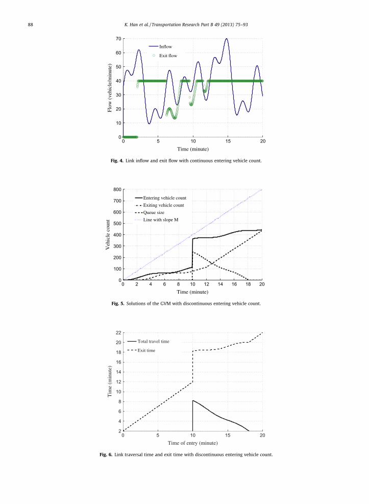
We consider a single link with bottleneck capacity M = 40 (in vehicle/min) and a free-flow travel time t0 = 2 (in min). Inorder to observe the performance of our algorithm under complex inflow profiles, we choose the link inflow function that israndomly generated with trigonometric functions, see Fig. 4. We fix a time horizon of [0, 20] (in min) and a time grid of 800intervals.

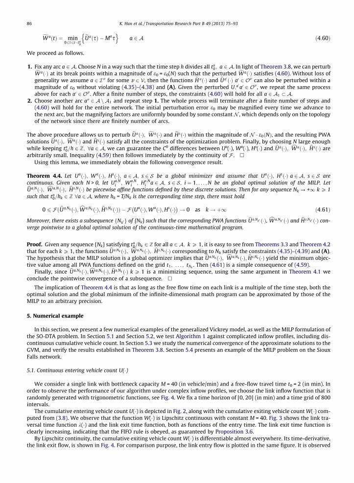
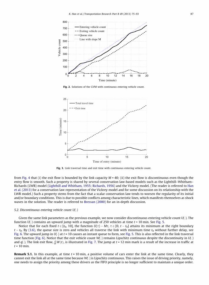
The cumulative entering vehicle count U(�) is depicted in Fig. 2, along with the cumulative exiting vehicle count W(�) com-puted from (3.8). We observe that the function W(�) is Lipschitz continuous with constant M = 40. Fig. 3 shows the link tra-versal time function k(�) and the link exit time function, both as functions of the entry time. The link exit time function isclearly increasing, indicating that the FIFO rule is obeyed, as guaranteed by Proposition 3.6.

By Lipschitz continuity, the cumulative exiting vehicle count W(�) is differentiable almost everywhere. Its time-derivative,the link exit flow, is shown in Fig. 4. For comparison purpose, the link entry flow is plotted in the same figure. It is observed

0 2 4 6 8 10 12 14 16 18 200

100

200

300

400

500

600

700

800

Time (minute)

Veh

icle

cou

nt

Entering vehicle count

Exiting vehicle count

Queue size

Line with slope M

Fig. 2. Solutions of the GVM with continuous entering vehicle count.

0 5 10 15 200

5

10

15

20

25

Time of entry (minute)

Tim

e (m

inut

e)

Total travel time

Exit time

Fig. 3. Link traversal time and exit time with continuous entering vehicle count.


from Fig. 4 that (i) the exit flow is bounded by the link capacity M = 40; (ii) the exit flow is discontinuous even though theentry flow is smooth. Such a property is shared by several conservation law-based models such as the Lighthill–Whitham–Richards (LWR) model (Lighthill and Whitham, 1955; Richards, 1956) and the Vickrey model. (The reader is referred to Hanet al. (2013) for a conservation law representation of the Vickrey model and for some discussion on its relationship with theLWR model.) Such a property stems from the fact that a scalar conservation law tends to worsen the regularity of its initialand/or boundary conditions. This is due to possible conflicts among characteristic lines, which manifests themselves as shockwaves in the solution. The reader is referred to Bressan (2000) for an in-depth discussion.

5.2. Discontinuous entering vehicle count U(�)

Given the same link parameters as the previous example, we now consider discontinuous entering vehicle count U(�). Thefunction U(�) contains an upward jump with a magnitude of 250 vehicles at time t = 10 min. See Fig. 5.

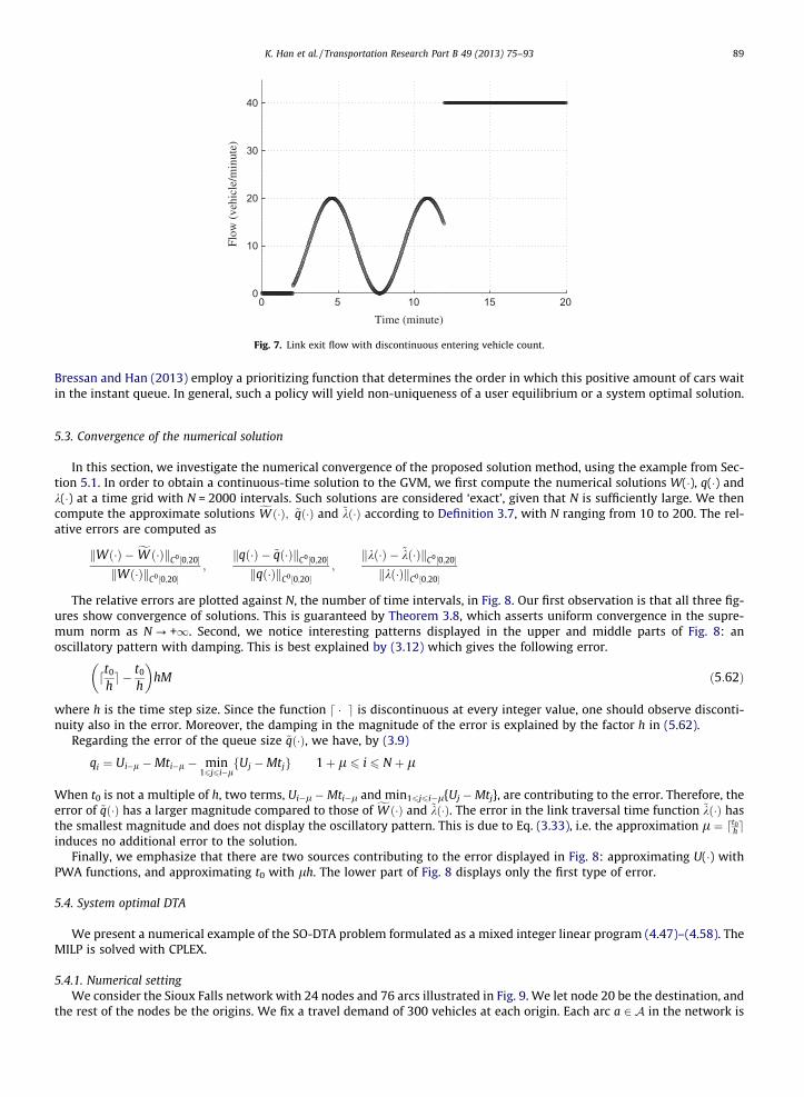
Notice that for each fixed t 2 [t0, 10], the function U(s) �Ms, s 2 [0, t � t0] attains its minimum at the right boundaryt � t0. By (3.6), the queue size is zero and vehicles all traverse the link with minimum time t0 without further delay, seeFig. 6. The upward jump in U(�) at t = 10 causes an instant queue to form, see Fig. 5. This is also reflected in the link traversaltime function (Fig. 6). Notice that the exit vehicle count W(�) remains Lipschitz continuous despite the discontinuity in U(�)and q(�). The link exit flow, d

dt WðtÞ, is illustrated in Fig. 7. The jump at t = 12 min mark is a result of the increase in traffic att = 10 min.

Remark 5.1. In this example, at time t = 10 min, a positive volume of cars enter the link at the same time. Clearly, theycannot exit the link all at the same time because W(�) is Lipschitz continuous. This raises the issue of driving priority, namely,one needs to assign the priority among these drivers as the FIFO principle is no longer sufficient to maintain a unique order.

0 5 10 15 200

10

20

30

40

50

60

70

Time (minute)

Flow

(ve

hicl

e/m

inut

e)

Inflow

Exit flow

Fig. 4. Link inflow and exit flow with continuous entering vehicle count.

0 2 4 6 8 10 12 14 16 18 200

100

200

300

400

500

600

700

800

Time (minute)

Veh

icle

cou

nt

Entering vehicle count

Exiting vehicle count

Queue size

Line with slope M

Fig. 5. Solutions of the GVM with discontinuous entering vehicle count.

0 5 10 15 202

4

6

8

10

12

14

16

18

20

22

Time of entry (minute)

Tim

e (m

inut

e)

Total travel time

Exit time

Fig. 6. Link traversal time and exit time with discontinuous entering vehicle count.


0 5 10 15 200

10

20

30

40

Time (minute)

Flow

(ve

hicl

e/m

inut

e)

Fig. 7. Link exit flow with discontinuous entering vehicle count.


Bressan and Han (2013) employ a prioritizing function that determines the order in which this positive amount of cars waitin the instant queue. In general, such a policy will yield non-uniqueness of a user equilibrium or a system optimal solution.

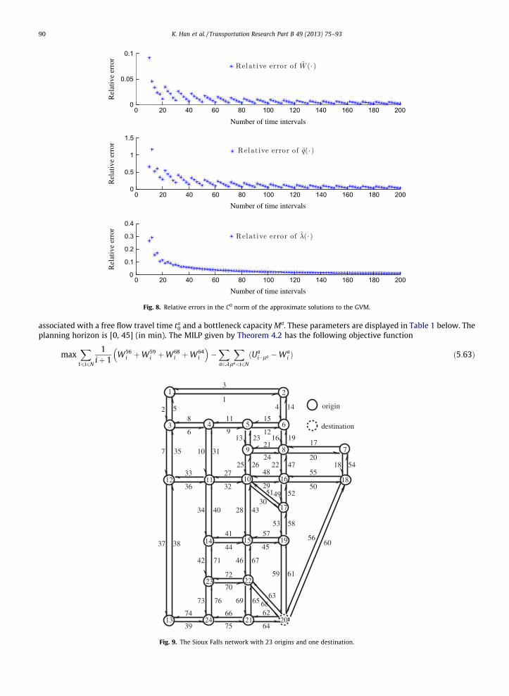
5.3. Convergence of the numerical solution

In this section, we investigate the numerical convergence of the proposed solution method, using the example from Sec-tion 5.1. In order to obtain a continuous-time solution to the GVM, we first compute the numerical solutions W(�), q(�) andk(�) at a time grid with N = 2000 intervals. Such solutions are considered ‘exact’, given that N is sufficiently large. We thencompute the approximate solutions fW ð�Þ; ~qð�Þ and ~kð�Þ according to Definition 3.7, with N ranging from 10 to 200. The rel-ative errors are computed as

kWð�Þ � fW ð�ÞkC0 ½0;20�

kWð�ÞkC0 ½0;20�;

kqð�Þ � ~qð�ÞkC0 ½0;20�

kqð�ÞkC0 ½0;20�;

kkð�Þ � ~kð�ÞkC0 ½0;20�

kkð�ÞkC0 ½0;20�

The relative errors are plotted against N, the number of time intervals, in Fig. 8. Our first observation is that all three fig-ures show convergence of solutions. This is guaranteed by Theorem 3.8, which asserts uniform convergence in the supre-mum norm as N ? +1. Second, we notice interesting patterns displayed in the upper and middle parts of Fig. 8: anoscillatory pattern with damping. This is best explained by (3.12) which gives the following error.

dt0

he � t0

h

� �hM ð5:62Þ

where h is the time step size. Since the function d � e is discontinuous at every integer value, one should observe disconti-nuity also in the error. Moreover, the damping in the magnitude of the error is explained by the factor h in (5.62).

Regarding the error of the queue size ~qð�Þ, we have, by (3.9)

qi ¼ Ui�l �Mti�l � min16j6i�l

fUj �Mtjg 1þ l 6 i 6 N þ l

When t0 is not a multiple of h, two terms, Ui�l �Mti�l and min16j6i�l{Uj �Mtj}, are contributing to the error. Therefore, theerror of ~qð�Þ has a larger magnitude compared to those of fW ð�Þ and ~kð�Þ. The error in the link traversal time function ~kð�Þ hasthe smallest magnitude and does not display the oscillatory pattern. This is due to Eq. (3.33), i.e. the approximation l ¼ dt0

heinduces no additional error to the solution.

Finally, we emphasize that there are two sources contributing to the error displayed in Fig. 8: approximating U(�) withPWA functions, and approximating t0 with lh. The lower part of Fig. 8 displays only the first type of error.

5.4. System optimal DTA

We present a numerical example of the SO-DTA problem formulated as a mixed integer linear program (4.47)–(4.58). TheMILP is solved with CPLEX.

5.4.1. Numerical settingWe consider the Sioux Falls network with 24 nodes and 76 arcs illustrated in Fig. 9. We let node 20 be the destination, and

the rest of the nodes be the origins. We fix a travel demand of 300 vehicles at each origin. Each arc a 2 A in the network is

0 20 40 60 80 100 120 140 160 180 2000

0.05

0.1

Number of time intervals

Rel

ativ

e er

ror

0 20 40 60 80 100 120 140 160 180 2000

0.5

1

1.5


Rel

ativ

e er

ror

0 20 40 60 80 100 120 140 160 180 2000

0.1

0.2

0.3

0.4


Rel

ativ

e er

ror

Fig. 8. Relative errors in the C0 norm of the approximate solutions to the GVM.


associated with a free flow travel time ta0 and a bottleneck capacity Ma. These parameters are displayed in Table 1 below. The

planning horizon is [0, 45] (in min). The MILP given by Theorem 4.2 has the following objective function

maxX

16i6N

1iþ 1

W56i þW59

i þW68i þW64

i

��Xa2A

Xla<i6N

ðUai�la �Wa

i Þ ð5:63Þ

3 4 5 6

9

3

12

8

6

47

5

1 2

7 10

12 11 10 16

49

13 23 16 1921

2452 26

2951

8

36 32

483322

7

18

20

17

50

5518 54

13

23

14 15 19

22

24 21 2074 66

75

62

64

37 76 69

42

59

6563

40 2843

71

4330

53 58

61

52

17

5660

46 67

68

73 83

3135

4 14

12

15

27

9

11

45

5741

44

72

70

39

origin

destination

Fig. 9. The Sioux Falls network with 23 origins and one destination.

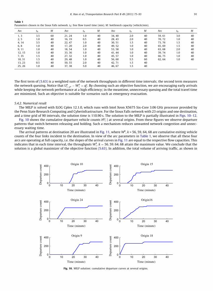
Table 1Parameters chosen in the Sioux Falls network. t0: free flow travel time (min). M: bottleneck capacity (vehicle/min).

Arc t0 M Arc t0 M Arc t0 M Arc t0 M

1, 3 3.5 60 21, 24 1.0 40 34, 40 2.0 40 59, 61 3.0 402, 5 1.0 40 16, 19 0.5 40 28, 43 2.0 40 70, 72 1.0 404, 14 3.5 40 22, 47 1.0 40 30, 51 1.5 40 73, 76 1.5 406, 8 1.0 40 17, 20 2.0 40 49, 52 1.0 40 65, 69 1.5 409, 11 1.0 40 18, 54 1.0 40 53, 58 1.0 40 63, 68 2.0 4012, 15 1.0 40 33, 36 1.0 40 41, 44 1.0 40 39, 74 1.0 407, 35 1.5 40 27, 32 1.0 40 45, 57 1.0 40 66, 75 1.0 4010, 31 1.5 40 29, 48 1.0 40 56, 60 5.5 60 62, 64 1.0 4013, 23 0.5 40 50, 55 2.0 40 42, 71 1.5 4025, 26 1.0 40 37, 38 5.0 40 46, 67 1.5 40


The first term of (5.63) is a weighted sum of the network throughputs in different time intervals; the second term measuresthe network queuing. Notice that Ua

i�la �Wai ¼ qa

i . By choosing such an objective function, we are encouraging early arrivalswhile keeping the network performance at a high efficiency; in the meantime, unnecessary queuing and the total travel timeare minimized. Such an objective is suitable for scenarios such as emergency evacuation.

5.4.2. Numerical resultThe MILP is solved with ILOG Cplex 12.1.0, which runs with Intel Xeon X5675 Six-Core 3.06 GHz processor provided by

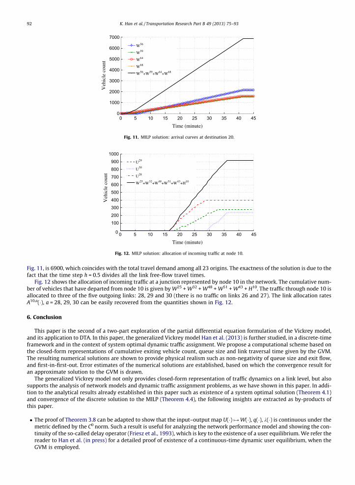
the Penn State Research Computing and Cyberinfrastructure. For the Sioux Falls network with 23 origins and one destination,and a time grid of 90 intervals, the solution time is 110.90 s. The solution to the MILP is partially illustrated in Figs. 10–12.

Fig. 10 shows the cumulative departure vehicle counts Hs(�) at several origins. From these figures we observe departurepatterns that switch between releasing and holding. Such a mechanism reduces unwanted network congestion and unnec-essary waiting time.

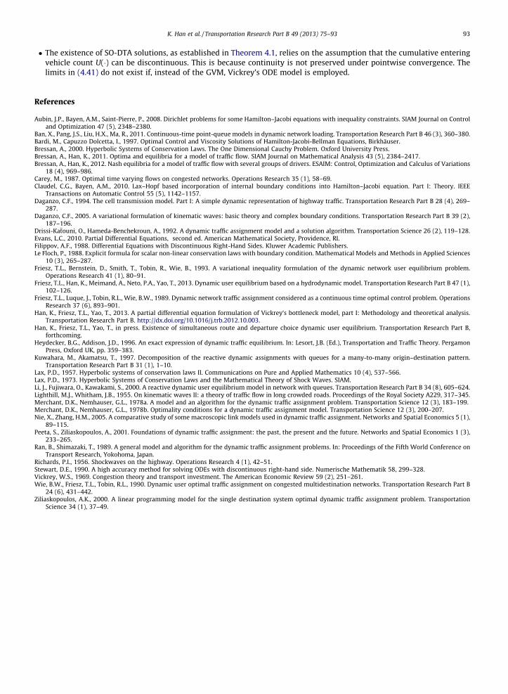
The arrival patterns at destination 20 are illustrated in Fig. 11, where Wk, k = 56, 59, 64, 68 are cumulative exiting vehiclecounts of the four links incident to the destination. In view of the arc parameters in Table 1, we observe that all these fourarcs are operating at full capacity, i.e. the slopes of the arrival curves in Fig. 11 are equal to the respective flow capacities. Thisindicates that in each time interval, the throughputs Wk

i ; k ¼ 56;59;64;68 attain the maximum value. We conclude that thesolution is a global maximizer of the objective function (5.63). In addition, the total volume of arriving traffic, as shown in

0 10 20 30 400

200

400

Time (minute)

Origin 10

0 10 20 30 400

200

400

Time (minute)

Dep

artu

re c

ount Origin 15

0 10 20 30 400

200

400

Time (minute)

Origin 24

0 10 20 30 400

200

400

Time (minute)

Dep

artu

re c

ount

Origin16

0 10 20 30 400

200

400

Time (minute)

Origin 9

0 10 20 30 400

200

400

Time (minute)

Dep

artu

re c

ount

Dep

artu

re c

ount

Dep

artu

re c

ount

Dep

artu

re c

ount

Origin 18

Fig. 10. MILP solution: cumulative departure curves at several origins.

0 5 10 15 20 25 30 35 40 450

1000

2000

3000

4000

5000

6000

7000

Time (minute)

Veh

icle

cou

nt

W56

W59

W64

W68

W56+W59+W64+W68

Fig. 11. MILP solution: arrival curves at destination 20.

0 5 10 15 20 25 30 35 40 450

1002003004005006007008009001000

Time (minute)

Veh

icle

cou

nt

U29

U30

U28

W25+W32+W48+W51+W43+H10

Fig. 12. MILP solution: allocation of incoming traffic at node 10.


Fig. 11, is 6900, which coincides with the total travel demand among all 23 origins. The exactness of the solution is due to thefact that the time step h = 0.5 divides all the link free-flow travel times.

Fig. 12 shows the allocation of incoming traffic at a junction represented by node 10 in the network. The cumulative num-ber of vehicles that have departed from node 10 is given by W25 + W32 + W48 + W51 + W43 + H10. The traffic through node 10 isallocated to three of the five outgoing links: 28, 29 and 30 (there is no traffic on links 26 and 27). The link allocation ratesA10,a(�), a = 28, 29, 30 can be easily recovered from the quantities shown in Fig. 12.

6. Conclusion

This paper is the second of a two-part exploration of the partial differential equation formulation of the Vickrey model,and its application to DTA. In this paper, the generalized Vickrey model Han et al. (2013) is further studied, in a discrete-timeframework and in the context of system optimal dynamic traffic assignment. We propose a computational scheme based onthe closed-form representations of cumulative exiting vehicle count, queue size and link traversal time given by the GVM.The resulting numerical solutions are shown to provide physical realism such as non-negativity of queue size and exit flow,and first-in-first-out. Error estimates of the numerical solutions are established, based on which the convergence result foran approximate solution to the GVM is drawn.

The generalized Vickrey model not only provides closed-form representation of traffic dynamics on a link level, but alsosupports the analysis of network models and dynamic traffic assignment problems, as we have shown in this paper. In addi-tion to the analytical results already established in this paper such as existence of a system optimal solution (Theorem 4.1)and convergence of the discrete solution to the MILP (Theorem 4.4), the following insights are extracted as by-products ofthis paper.

� The proof of Theorem 3.8 can be adapted to show that the input–output map U(�) ´ W(�), q(�), k(�) is continuous under themetric defined by the C0 norm. Such a result is useful for analyzing the network performance model and showing the con-tinuity of the so-called delay operator (Friesz et al., 1993), which is key to the existence of a user equilibrium. We refer thereader to Han et al. (in press) for a detailed proof of existence of a continuous-time dynamic user equilibrium, when theGVM is employed.


� The existence of SO-DTA solutions, as established in Theorem 4.1, relies on the assumption that the cumulative enteringvehicle count U(�) can be discontinuous. This is because continuity is not preserved under pointwise convergence. Thelimits in (4.41) do not exist if, instead of the GVM, Vickrey’s ODE model is employed.

References

Aubin, J.P., Bayen, A.M., Saint-Pierre, P., 2008. Dirichlet problems for some Hamilton–Jacobi equations with inequality constraints. SIAM Journal on Controland Optimization 47 (5), 2348–2380.

Ban, X., Pang, J.S., Liu, H.X., Ma, R., 2011. Continuous-time point-queue models in dynamic network loading. Transportation Research Part B 46 (3), 360–380.Bardi, M., Capuzzo Dolcetta, I., 1997. Optimal Control and Viscosity Solutions of Hamilton-Jacobi-Bellman Equations, Birkhäuser.Bressan, A., 2000. Hyperbolic Systems of Conservation Laws. The One Dimensional Cauchy Problem. Oxford University Press.Bressan, A., Han, K., 2011. Optima and equilibria for a model of traffic flow. SIAM Journal on Mathematical Analysis 43 (5), 2384–2417.Bressan, A., Han, K., 2012. Nash equilibria for a model of traffic flow with several groups of drivers. ESAIM: Control, Optimization and Calculus of Variations

18 (4), 969–986.Carey, M., 1987. Optimal time varying flows on congested networks. Operations Research 35 (1), 58–69.Claudel, C.G., Bayen, A.M., 2010. Lax–Hopf based incorporation of internal boundary conditions into Hamilton–Jacobi equation. Part I: Theory. IEEE

Transactions on Automatic Control 55 (5), 1142–1157.Daganzo, C.F., 1994. The cell transmission model. Part I: A simple dynamic representation of highway traffic. Transportation Research Part B 28 (4), 269–

287.Daganzo, C.F., 2005. A variational formulation of kinematic waves: basic theory and complex boundary conditions. Transportation Research Part B 39 (2),

187–196.Drissi-Katouni, O., Hameda-Benchekroun, A., 1992. A dynamic traffic assignment model and a solution algorithm. Transportation Science 26 (2), 119–128.Evans, L.C., 2010. Partial Differential Equations, second ed. American Mathematical Society, Providence, RI.Filippov, A.F., 1988. Differential Equations with Discontinuous Right-Hand Sides. Kluwer Academic Publishers.Le Floch, P., 1988. Explicit formula for scalar non-linear conservation laws with boundary condition. Mathematical Models and Methods in Applied Sciences

10 (3), 265–287.Friesz, T.L., Bernstein, D., Smith, T., Tobin, R., Wie, B., 1993. A variational inequality formulation of the dynamic network user equilibrium problem.

Operations Research 41 (1), 80–91.Friesz, T.L., Han, K., Meimand, A., Neto, P.A., Yao, T., 2013. Dynamic user equilibrium based on a hydrodynamic model. Transportation Research Part B 47 (1),

102–126.Friesz, T.L., Luque, J., Tobin, R.L., Wie, B.W., 1989. Dynamic network traffic assignment considered as a continuous time optimal control problem. Operations

Research 37 (6), 893–901.Han, K., Friesz, T.L., Yao, T., 2013. A partial differential equation formulation of Vickrey’s bottleneck model, part I: Methodology and theoretical analysis.

Transportation Research Part B. http://dx.doi.org/10.1016/j.trb.2012.10.003.Han, K., Friesz, T.L., Yao, T., in press. Existence of simultaneous route and departure choice dynamic user equilibrium. Transportation Research Part B,

forthcoming.Heydecker, B.G., Addison, J.D., 1996. An exact expression of dynamic traffic equilibrium. In: Lesort, J.B. (Ed.), Transportation and Traffic Theory. Pergamon

Press, Oxford UK, pp. 359–383.Kuwahara, M., Akamatsu, T., 1997. Decomposition of the reactive dynamic assignments with queues for a many-to-many origin–destination pattern.

Transportation Research Part B 31 (1), 1–10.Lax, P.D., 1957. Hyperbolic systems of conservation laws II. Communications on Pure and Applied Mathematics 10 (4), 537–566.Lax, P.D., 1973. Hyperbolic Systems of Conservation Laws and the Mathematical Theory of Shock Waves. SIAM.Li, J., Fujiwara, O., Kawakami, S., 2000. A reactive dynamic user equilibrium model in network with queues. Transportation Research Part B 34 (8), 605–624.Lighthill, M.J., Whitham, J.B., 1955. On kinematic waves II: a theory of traffic flow in long crowded roads. Proceedings of the Royal Society A229, 317–345.Merchant, D.K., Nemhauser, G.L., 1978a. A model and an algorithm for the dynamic traffic assignment problem. Transportation Science 12 (3), 183–199.Merchant, D.K., Nemhauser, G.L., 1978b. Optimality conditions for a dynamic traffic assignment model. Transportation Science 12 (3), 200–207.Nie, X., Zhang, H.M., 2005. A comparative study of some macroscopic link models used in dynamic traffic assignment. Networks and Spatial Economics 5 (1),

89–115.Peeta, S., Ziliaskopoulos, A., 2001. Foundations of dynamic traffic assignment: the past, the present and the future. Networks and Spatial Economics 1 (3),

233–265.Ran, B., Shimazaki, T., 1989. A general model and algorithm for the dynamic traffic assignment problems. In: Proceedings of the Fifth World Conference on

Transport Research, Yokohoma, Japan.Richards, P.I., 1956. Shockwaves on the highway. Operations Research 4 (1), 42–51.Stewart, D.E., 1990. A high accuracy method for solving ODEs with discontinuous right-hand side. Numerische Mathematik 58, 299–328.Vickrey, W.S., 1969. Congestion theory and transport investment. The American Economic Review 59 (2), 251–261.Wie, B.W., Friesz, T.L., Tobin, R.L., 1990. Dynamic user optimal traffic assignment on congested multidestination networks. Transportation Research Part B

24 (6), 431–442.Ziliaskopoulos, A.K., 2000. A linear programming model for the single destination system optimal dynamic traffic assignment problem. Transportation

Science 34 (1), 37–49.


A partial differential equation formulation of Vickrey’s bottleneck model, part II: Numerical...

Documents

Transcript of A partial differential equation formulation of Vickrey’s bottleneck model, part II: Numerical...