Analysis of a Multiserver Queue with Setup Times

Queueing Systems 52, 53–76, 2005c© 2005 Springer Science + Business Media, Inc. Manufactured in The Netherlands.

Analysis of a Multiserver Queue with Setup Times

J.R. ARTALEJODepartment of Statistics and O.R., Faculty of Mathematics, Complutense University of Madrid, Madrid28040, Spain

A. ECONOMOUDepartment of Mathematics, University of Athens, Panepistemioupolis, Athens 15784, Greece

M.J. LOPEZ-HERREROSchool of Statistics, Complutense University of Madrid, Madrid 28040, Spain

Received 7 May 2004; Revised 20 April 2005

Abstract. This paper deals with the analysis of an M/M/c queueing system with setup times. This queueingmodel captures the major characteristics of phenomena occurring in production when the system consists ina set of machines monitored by a single operator. We carry out an extensive analysis of the system includinglimiting distribution of the system state, waiting time analysis, busy period and maximum queue length.

Keywords: queueing performance, multiserver queue, setup times, continuous time Markov chain, differ-ence equations, matrix geometric solutions, numerical inversion

AMS subject classification: 90B22, 60K25

1. Introduction

Queues with removable servers (or vacation models) where the servers may be unavail-able for serving customers over some intervals of time have been the subject matter ofmany papers, mainly due to their versatility and applicability in a variety of computer,communication and production systems. The literature concerning the single servercase is extremely vast. For the multiserver case the number of published papers is moremoderate. A classification of most of them is done in [4].

In this context, many papers are dedicated to the analysis of single server queueswith setup times, for instance, see [6,8,9,11,12] and the references therein. In contrast,we have been able to find only one paper by Borthakur and Choudhury [7] concerninga multiserver queue with setup times. In [7] the authors consider a system where allthe servers are simultaneously turned off as soon as the system becomes empty. Theservers remain inactive until N ≥ c customers are accumulated. Then a start up periodbegins in order to make the system operative. Our paper also deals with a multiserverqueue with setup times but the operating rules governing our model differ substantiallyof those considered in [7].

54 ARTALEJO, ECONOMOU AND LOPEZ-HERRERO

Our model is motivated by situations arising in production systems where severalidentical machines process jobs in order of their arrivals. To save running costs whilethere are no jobs, the machines are switched off as soon as the queue is empty. A setuptime is needed to turn on a machine again. Since the system is monitored by a singleoperator, we assume that at most one machine is warming up at any time t. A similarqueueing system is proposed by Adan and van der Wal [2] for modelling a productionsystem where a single machine provides service to pending jobs.

As usual, a first step in our analysis will be the study of the stationary system statedistribution. However, our aim is to provide a much more detailed study of the systemperformance. To this end, we will investigate the waiting time, the length of a busyperiod and the maximum queue length observed. We will provide a route of evaluationfor these queueing distributions by putting emphasis on a difference equations approach(for a detailed exposition see [10]) which is supplemented by a variety of well-knownmathematical tools such as matrix-analytic methods and numerical inversion.

More concretely, our main goals in this paper can be summarized as follows:

(a) To study the stationary distribution of the system state using a difference equationsapproach. The resulting expressions are related to the matrix-analytic approach.

(b) To investigate the waiting time distribution of a customer. Using the results on thestationary distribution of the system and employing a technique of Bertsimas [5], weobtain explicitly both the unconditional distribution and the conditional distributiongiven that the customer finds all the servers active. Moreover, given the systemstate upon arrival, we reduce the study of the conditional waiting time to a firstpassage problem which can be investigated by combining difference equations andnumerical inversion techniques.

(c) To analyze the busy period and the maximum queue length observed. The differenceequations approach yields again tractable expressions. Our numerical examples arefocused on the numerical inversion of the length of a busy period and the computationof the distribution of the maximum queue length.

As related work, we first mention the existing literature devoted to single serverqueues with setup times and the papers dealing with multiple removable servers. Thelatter are characterized by bidimensional representations of the system state (for exam-ple, see [13] which is one of the pioneering works on this topic). In this way, our workalso connects with the abundant literature for two-dimensional queueing systems. Arecent example is the model with gated random order of service investigated by Resingand Rietman [16]. To illustrate the application of the difference equations approach, orspectral expansion method, to other stochastic models we mention the inventory systemstudied by Adan and van der Wal [1].

The rest of the paper is organized as follows. In Section 2, we describe the math-ematical model as a quasi-birth-and-death (QBD) process. In Section 3, we use thedifference equations approach to study the stationary distribution of the system stateand we relate it with the matrix-analytic theory. The analysis of the waiting time is

ANALYSIS OF A MULTISERVER QUEUE WITH SETUP TIMES 55

Figure 1. States and transitions.

presented in Section 4. Next, in Section 5 we deal with the analysis of the busy periodand related quantities. Numerical examples are given in several points along the paper.There is also an Appendix, where we report some results which proof is omitted.

2. Model description

We consider a multiserver queueing system in which customers arrive according to aPoisson process with rate λ. Customers are served by c identical servers and the servicetimes are exponentially distributed with rate μ. The servers are turned off as soon asthe queue becomes empty. The active servers offer service under first-come-first-serveddiscipline. When a new customer arrives and finds at least one free server which is turnedoff, the administrator of the system prepares one server but it takes an exponential setuptime with rate θ . We assume the case where several pending setup times are not allowed,i.e., the administrator prepares servers one by one until the queue becomes empty. In casethat at any service completion epoch the queue reduces to a single customer, the setup inprogress is stopped and the waiting customer automatically starts to be served. We alsoassume that interarrival times, service times and setup times are mutually independent.In figure 1, we show the transitions among states in our multiserver queue with setuptimes.

We represent the state of the system at time t by the pair (S(t), N (t)), whereS(t) is the number of active servers and N (t) denotes the total number of customersin the system. The process {(S(t), N (t)); t ≥ 0} is a QBD process with state spaceS = {(i, n)|0 ≤ i ≤ c, n ≥ i}. At the light of figure 1 we observe that startingfrom a non-boundary state (i, n) is not possible to make transitions to states ( j, m)


with j < i without going through the boundary states (k, k), j ≤ k ≤ i . Due to thisspecial structure, we will be able to obtain tractable solutions for many performancecharacteristics. Replacing N (t) by the number of waiting customers M(t) (i.e., we haveM(t) = N (t) − S(t)), we obtain an alternative representation. This remark due to areferee yields a simpler state space in a standard semi-infinite strip. Both formulationsare valid and equivalent. We still keep the original one which also shows that a similaranalysis could be performed for other QBD processes with a large number of boundarystates.

Our whole analysis can be also applied in the case where multiple server initial-izations are allowed. In that case, we only need to adapt the rates that correspond to thecompletion of setup times. Assuming that at most k servers can be initialized simulta-neously, the setup rate for state (i, n) is min(n − i, c − i, k)θ . We choose to present thecase k = 1, since the overall notation becomes much simpler. However, the analysisremains the same with appropriate modifications.

3. System state distribution

The first question to be investigated concerns the limiting probabilities

xin = limt→∞ P{(S(t), N (t)) = (i, n)}, (i, n) ∈ S,

which satisfy the following balance equations

λx00 = μx11, (1)

(λ + θ )x0n = λx0,n−1, n ≥ 1, (2)

(λ + iμ)xii = θxi−1,i + iμxi,i+1 + (i + 1)μxi+1,i+1, 1 ≤ i ≤ c − 1, (3)

(λ + iμ + θ )xin = θxi−1,n + λxi,n−1 + iμxi,n+1, 1 ≤ i ≤ c − 1, n ≥ i + 1, (4)

(λ + cμ)xcc = θxc−1,c + cμxc,c+1, (5)

(λ + cμ)xcn = θxc−1,n + λxc,n−1 + cμxc,n+1, n ≥ c + 1, (6)

and the normalizing condition

c∑i=0

∞∑n=i

xin = 1. (7)

The tractability of this system lies in the fact that it is a QBD whose rate matrixR is obtained as the minimal solution of the equation R2A2 + RA1 + A0 = 0, wherethe underlying block matrices Ak, 0 ≤ k ≤ 2, and hence also R, are upper triangular(see Sections 1.4 and 6.5 in [15]). As a result of this, the matrix R can be determinedrecursively, i.e., we avoid to compute R by successive iterations. The eigenvaluesϕi of thematrix R are its diagonal elements rii . They can be obtained as the smallest nonnegativesolutions of the equations iμx2 − (λ + iμ + θ1{i < c})x + λ = 0, 0 ≤ i ≤ c, where


1{i < c} denotes the indicator function of the subset {i < c}. Hence

ϕ0 = λ

λ + θ, (8)

ϕi = λ + iμ + θ −√

(λ + iμ + θ )2 − 4λiμ2iμ

, 1 ≤ i ≤ c − 1,

and

ϕc = min

(λ

cμ, 1

).

Once the eigenvalues are known, we notice that the rest of the elements of thematrix R can be recursively computed from the formula

jμj∑

k=i

rikrk j + θri, j−1 − (λ + jμ + θ1{ j < c})ri j = 0, 0 ≤ i ≤ c − 1, i + 1 ≤ j ≤ c.

We also observe that ϕi ∈ (0, 1), for 0 ≤ i ≤ c − 1. Therefore the positiverecurrence of the process {(S(t), N (t)); t ≥ 0}, which is equivalent to the spectral radiusof R being less than 1, holds if and only if ϕc < 1, i.e., whenever λ < cμ. In what followswe assume this stability condition. Moreover, it is easy to prove that all ϕi , 0 ≤ i ≤ c−1,are different. In addition, for any k ∈ {0, . . . , c − 1}, we can prove that ϕk = ϕc if andonly if θc = (cμ − λ)(c − k). This discussion forces us to distinguish two cases in thefollowing theorem.

Theorem 1.

Case I: ϕi �= ϕc, for all i = 0, . . . , c − 1.The limiting probabilities xin are given by

x00 =(

c∑i=0

i∏k=0

γk

i∑j=0

αi j

1 − ϕ j

)−1

, (9)

xii = x00

i∏k=0

γk, 1 ≤ i ≤ c, (10)

xin = xii

i∑j=0

αi jϕn−ij , 0 ≤ i ≤ c, n ≥ i, (11)

where the coefficients γi , 0 ≤ i ≤ c, and αi j , 0 ≤ j ≤ i ≤ c, are computed by therecursive scheme

γ0 = α00 = 1, (12)


γi = 1

iμ

(λ + (i − 1)μ − (i − 1)μ

i−1∑j=0

αi−1, jϕ j −i−2∑j=0

(i − 1 − j)μαi−1, j (1 − ϕ j )

)

> 0, 1 ≤ i ≤ c, (13)

αi j = θαi−1, jϕ j

(i − j)μ(1 − ϕ j )γi, 1 ≤ i ≤ c − 1, 0 ≤ j ≤ i − 1, (14)

αcj = θαc−1, jϕ j

((c − j)μ(1 − ϕ j ) − θ )γc, 0 ≤ j ≤ c − 1, (15)

αi i = 1 −i−1∑j=0

αi j , 1 ≤ i ≤ c. (16)

Case II: ϕk = ϕc, for some k ∈ {0, . . . , c − 1}.Then the limiting probabilities xin have the structural form (9)–(11) except x00 andxcn which are given by

x00 =(

αckϕk

(1 − ϕk)2

c∏k=0

γk +c∑

i=0

i∏k=0

γk

i∑j=0

αi j

1 − ϕ j

)−1

,

xcn = xcc

((n − c)αckϕ

n−ck +

c∑j=0

αcjϕn−cj

), n ≥ c,

where the coefficients γi , 0 ≤ i ≤ c, and αi j , 0 ≤ j ≤ i ≤ c, are given in (12)–(16)except αck which now is

αck = θαc−1,kϕ2k

λ − cμϕ2k

.

Proof. For brevity, we present only the proof for Case I. By combining (2), (8) and(12) we trivially find that

x0n = x00α00ϕn0 , n ≥ 0,

which agrees with formula (11) for i = 0. From equations (1), (12) and (13), we alsosee that expression (10) holds for i = 1.

Suppose now by the inductive hypothesis that x1n, . . . , xi−1,n have the form (10)–(11), for some i ≤ c − 1 and moreover that all the required coefficients γ0, · · · , γi−1

are positive. Let us consider formula (3) for i − 1. By the inductive hypothesis we havexi−1,i−1 = γi−1xi−2,i−2, for 1 < i ≤ c − 1, and appropriate expressions for xi−2,i−1 and


xi−1,i . This yields the expression

xii = xi−2,i−2

iμ

((λ + (i − 1)μ)γi−1 − θ

i−2∑j=0

αi−2, jϕ j − (i − 1)μγi−1

i−1∑j=0

αi−1, jϕ j

)

= γiγi−1xi−2,i−2,

where for the last equality we have used (14) for i − 1. This expression implies that γiis positive since xii , being a stationary probability of the irreducible positive recurrentchain {(S(t), N (t)); t ≥ 0}, is positive. So we can now safely define αi j , 0 ≤ j ≤ i − 1,by (14) and we have also that xii = γi xi−1,i−1. Hence (10) is valid for i ≤ c − 1. Nowwe will prove the validity of (11).

During the inductive step the variable i is fixed, so for notational convenience wesimply denote xn = xin, n ≥ i . We observe by (4) that xn satisfies the linear differenceequation

−iμxn+1 + (λ + iμ + θ )xn − λxn−1 = θxi−1,n, n ≥ i + 1. (17)

The solution of the associated homogeneous equation yields

c1ρn1 + c2ρ

n2 ,

where ρ1 and ρ2 are the roots of the characteristic equation

iμx2 − (λ + iμ + θ )x + λ = 0.

Thus, we have ρ1 = ϕi and

ρ2 = λ + iμ + θ +√

(λ + iμ + θ )2 − 4λiμ2iμ

Hence, the general solution of (17), given that τn is a particular solution, has theform

c1ρn1 + c2ρ

n2 + τn. (18)

After some algebra, it is possible to prove that

τn = xii

i−1∑j=0

αi jϕn−ij , n ≥ i, (19)

where αi j , 0 ≤ j ≤ i − 1, are computed from (14), is the desired particular solution.Since ρ2 > 1 we easily conclude that c2 = 0. Putting n = i into (18) gives

c1 = ϕ−ii

(1 −

i−1∑j=0

αi j

)xii . (20)


Combining (18)–(20) we complete the induction, so expression (11) for xin holdsfor i ≤ c − 1.

Now we turn our interest to the case i = c. The validity of expression (10) forxcc is consequence of repeating the arguments given at the beginning of the proof fori ≤ c − 1. Let us set yn = xcn, n ≥ c. Then, by equation (6) we have

−cμyn+1 + (λ + cμ)yn − λyn−1 = θxc−1,n, n ≥ c + 1. (21)

In this case we can prove that ϕc and 1 are the distinct roots of the characteris-tic function associated to the corresponding homogeneous equation. Thus, the generalsolution of (21) is

c′1ϕ

nc + c′

2 + σn, (22)

where σn is a particular solution of (21). After some algebra we may verify that

σn = xcc

c−1∑j=0

αcjϕn−cj , n ≥ c, (23)

satisfy the non-homogeneous equation (21). It should be stressed that the assumptionϕi �= ϕc, for all i = 0, . . . , c − 1, plays an essential role to determine that αcj is as weclaimed in (15).

Because of the normalizing condition (7) we should have c′2 = 0. In addition, by

putting n = c in (22) we obtain that

c′1 = ϕ−c

c

(1 −

c−1∑j=0

αcj

)xcc. (24)

Substituting (23)–(24) into (22) we prove the validity of (11) for i = c.The proof for the Case II follows a parallel scheme. The main differences concern

with the choice of the particular solution of equation (21).

Let xn be the row vector that contains the limiting probabilities associated to thelevel n of the QBD (i.e., the subset Sn = {(i, n)|0 ≤ i ≤ min(n, c)}, n ≥ 0). At this point,we refer the reader to Section 1.6 in [15] where the relation between the matrix-geometricsolution (see Theorem 1.7.1 in [15]) and the spectral expansion formulation is clearlystated. In fact, the solution in Theorem 1 can be interpreted in terms of formula (1.6.1)in [15], where xn is reduced to finite sums involving the eigenvalues and eigenvectorsof R.

More precisely, by interpreting Theorem 1 (i.e., the difference equations solutionor spectral expansion form) in terms of the matrix-geometric form we have that xn =xcRn−c, n ≥ c, where the Jordan canonical form M−1DM of R, is explicitly known.Indeed, in Case I, D is the diagonal matrix with diagonal elements ϕi , 0 ≤ i ≤ c, andM = (m ji ) is the triangular matrix with elements m ji = αi jϕ

−ij

∏ik=0 γk , for j ≤ i .

Similarly, in Case II, we have that D is the Jordan matrix with diagonal elements ϕi , 0 ≤


i ≤ c and dkc = 1. The matrix M has its c first columns identical to the correspondingones in Case I, while the last column differs only in the entries (k, c) and (c, c) whichare given by mkc = ((1 − ϕc − c)αck + αcc)ϕ−c

c∏c

l=0 γl and mcc = αckϕ−c+1c

∏cl=0 γl .

4. Waiting time analysis

In this section we turn our attention to the waiting time which is defined as the sojourntime of a customer in the queue excluding the service time. Since the arrival processis Poisson, we may appeal to PASTA (Poisson arrivals see time averages) property toconclude that the distribution of the unconditional waiting time, W, is a mixture ofthe distributions of the conditional waiting times, W(i,n), given that the tagged arrivingcustomer finds the system at state (i, n−1). Then, for the corresponding Laplace-Stieltjestransforms, we get

W (s) =c∑

i=0

∞∑n=i+1

xi,n−1W (i,n)(s). (25)

It should be pointed out that W(i,n) does not depend on future arrivals occurringafter the arrival time of the marked customer. In fact, by neglecting the events associatedto the Poisson arrival process, we can view W(i,n) as the first passage time from theinitial state (i, n) to the subset {(k, k)|i ≤ k ≤ c}. We next use first step analysis toobtain the system of equations governing the dynamics of the transforms W (i,n)(s). Thiswell-known methodology has also been successfully employed to investigate the waitingtime of other bidimensional Markovian systems (see e.g. [3]).

By conditioning on the nearest future event and using Markov property and timehomogeneity, we obtain the system of equations

W (c,n)(s) = cμs + cμ

W (c,n−1)(s), n ≥ c + 1, (26)

W (i,n)(s) = iμs + iμ + θ

W (i,n−1)(s)

+ θ

s + iμ + θW (i+1,n)(s), 0 ≤ i ≤ c − 1, n ≥ i + 1, (27)

and the boundary conditions

W (i,i)(s) = 1, 1 ≤ i ≤ c. (28)

The system (26)–(28) can be solved by using the method of difference equations.The recursive solution is given in Theorem 4 of the Appendix.

An interesting question is to investigate whether the waiting time distributioncan be determined explicitly in the form of a mixture of exponential contributions.Bertsimas [5] gives a closed form solution of this type for a class of G/G/c queueing


systems operating under FCFS discipline. Specifically, the interarrival and service timesfollow mixed generalized Erlang distributions which can approximate arbitrarily closeany general distribution. It should be pointed out that the class of queueing systemsinvestigated by Bertsimas [5] operates under FCFS discipline so the waiting time of acustomer is fully determined upon arrival to the system. In contrast, the waiting time inour model depends on setup completions occurring whereas the tagged customer waitsat the queue. Despite of this fact, the next result shows that the unconditional waitingtime distribution takes the form of a mixture of exponential and Erlang distributions.

Theorem 2. Let us assume that ϕi �= ϕc, for all i = 0, . . . , c − 1.

Case A: ϕ j �= 1 − θ(c−l)μ , for all j = 0, . . . , c − 1 and l = j, . . . , c − 1.

The distribution function of W is given by

P{W ≤ t} =c−1∑i=0

i∑j=0

c−1∑l=i

xiiαi j Ail(ϕ j )

ϕi+1j

(lμ

(1 − ϕ j

) + θ)(

1 − e−(lμ(1−ϕ j )+θ )t)

+c∑

i=0

i∑j=0

xiiαi j Aic(ϕ j )

ϕi+1j cμ(1 − ϕ j )

(1 − e−cμ(1−ϕ j )t

). (29)

Case B: ϕ j = 1 − θ〈c−l〉μ , for some pair ( j, l) such that j = 0, . . . , c − 1 and l =

j, . . . , c − 1.The distribution function of W is given by

P{W ≤ t} =c−1∑i=0

i∑j=0

xiiαi j Aic(ϕ j )

ϕi+1j (cμ(1 − ϕ j ))2

(1 − e−cμ(1−ϕ j )t (1 + cμ(1 − ϕ j )t)

)

+c−1∑i=0

i∑j=0

c−1∑l=i

xiiαi j Ail(ϕ j )

ϕi+1j (lμ(1 − ϕ j ) + θ )

(1 − e−(lμ(1−ϕ j )+θ )t)

+c∑

j=0

xccαcj

1 − ϕ j

(1 − e−cμ(1−ϕ j )t

). (30)

The computation of the coefficients Ail(ϕ j ) will be discussed in the sequel.

Proof. For z ∈ (0, 1) we define the transforms

Pi (z, s) =∞∑

n=i+1

W (i,n)(s)zn, 0 ≤ i ≤ c.


Then equation (27) readily yields

Pi (z, s) = (iμ + θ )zi+1

s + iμ(1 − z) + θ+ θ

s + iμ(1 − z) + θPi+1(z, s), 0 ≤ i ≤ c − 1. (31)

Moreover, in the particular case where all the servers are busy, iterating formula(26) results in

W (c,n)(s) =(

cμs + cμ

)n−c

, n ≥ c. (32)

Thus, Pc(z, s) is given by

Pc(z, s) = cμzc+1

s + cμ(1 − z). (33)

Iterating (31) we find after some algebra that Pi (z, s) has the form

Pi (z, s) =c−1∑h=i

θh−i (hμ + θ )zh+1∏hl=i (s + lμ(1 − z) + θ )

+ θ c−i cμzc+1( ∏c−1l=i (s + lμ(1 − z) + θ )

)(s + cμ(1 − z))

= Ni (z, s)( ∏c−1l=i (s + lμ(1 − z) + θ )

)(s + cμ(1 − z))

, 0 ≤ i ≤ c − 1, (34)

where Ni (z, s) is a polynomial of s with degree smaller than the degree of the denomi-nator. The factors in the denominator are all different except in the case where for somel ∈ {i, . . . , c − 1} we have lμ(1 − z) + θ = cμ(1 − z), which occurs if and only ifz = 1 − θ

(c−l)μ . This motivates to consider the cases A and B.If all the factors in the denominator of (34) are different, we may consider the

partial fraction expansion

Pi (z, s) =c−1∑l=i

Ail(z)

s + lμ(1 − z) + θ+ Aic(z)

s + cμ(1 − z), 0 ≤ i ≤ c − 1. (35)

Note that the coefficients Ail(z) can be obtained using (34) as follows

Ail(z) = lims→−(lμ(1−z)+θ )

(s + lμ(1 − z) + θ )Pi (z, s), i ≤ l ≤ c − 1,

Aic(z) = lims→−cμ(1−z)

(s + cμ(1 − z))Pi (z, s).

We may use (25) and (11) to obtain

W (s) =c∑

i=0

i∑j=0

xiiαi j

ϕi+1j

Pi (ϕ j , s). (36)


Substituting (33) and (35) into (36), we find that

W (s) =c−1∑i=0

i∑j=0

c−1∑l=i

xiiαi j Ail(ϕ j )

ϕi+1j (s + lμ(1 − ϕ j ) + θ )

+c∑

i=0

i∑j=0

xiiαi j Aic(ϕ j )

ϕi+1j (s + cμ(1 − ϕ j ))

,

(37)

where Acc(ϕ j ) = cμϕc+1j , 0 ≤ j ≤ c. The inversion of formula (37) leads to the desired

expression (29).If z = 1 − θ

〈c−l0〉μ , then we replace expression (35) by

Pi (z, s) =c−1∑l=i

Ail(z)

s + lμ(1 − z) + θ+ Aic(z)

(s + cμ(1 − z))2, 0 ≤ i ≤ c − 1,

and the coefficients Aic(z) and Ail0 (z) are now calculated from the equations

Aic(z) = lims→−cμ(1−z)

(s + cμ(1 − z))2 Pi (z, s),

lims→0

Pi (z, s) =c−1∑l=i

Ail(z)

lμ(1 − z) + θ+ Aic(z)

(cμ(1 − z))2.

The rest of the proof follows parallel steps to those given in the case A, but now W (s)has also a term of the form (s + cμ(1 − ϕ j ))−2 which results to the Erlang contributionin the first term of the right hand side of formula (30) for P{W ≤ t}.

The above theorem only covers the Case I. The Case II (i.e., ϕk = ϕc, for somek ∈ {0, . . . , c − 1}) can be treated similarly.

In what follows, we turn to the conditional waiting times W(i,n). At the light offormula (32) we notice that the conditional waiting time W(c,n) has an Erlang distri-bution. However, for any arbitrary starting state (i, n), i < c, the analytical solutionseems intricate, so we use numerical inversion to compute the conditional waiting timedistributions. For notational convenience, we next denote the state after the arrival ofthe tagged customer as (i0, n0).

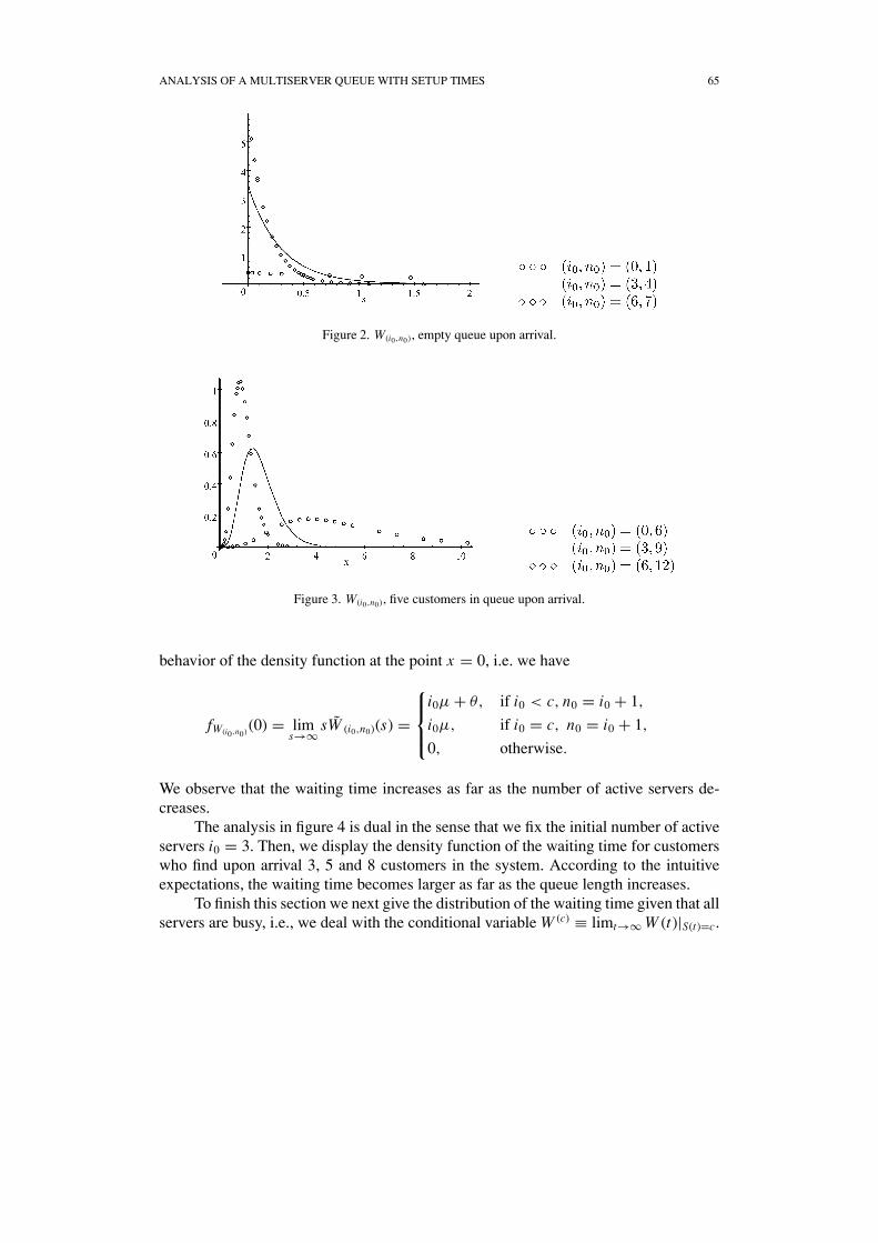
Figures 2–4 show the influence of the initial state (i0, n0) on the waiting time ofthe tagged customer. To this end, we consider c = 6, μ = 1 and θ = 0.4. Then, weuse Theorem 4 in the Appendix to compute the Laplace-Stieltjes transform W (i0,n0)(s).The numerical inversion of this transform leads to the density functions displayed in thefigures.

In figure 2, the tagged customer finds an empty queue upon arrival whereas infigure 3 he finds five customers waiting for service. In both cases, we display 3 curvescorresponding to the cases i0 = 0, 3, 6. The different shape of the densities in both figurescan be explained in terms of the Tauberian theorems which allow us to determine the


Figure 2. W(i0,n0), empty queue upon arrival.

Figure 3. W(i0,n0), five customers in queue upon arrival.

behavior of the density function at the point x = 0, i.e. we have

fW(i0,n0) (0) = lims→∞ sW (i0,n0)(s) =

⎧⎪⎨⎪⎩

i0μ + θ, if i0 < c, n0 = i0 + 1,

i0μ, if i0 = c, n0 = i0 + 1,

0, otherwise.

We observe that the waiting time increases as far as the number of active servers de-creases.

The analysis in figure 4 is dual in the sense that we fix the initial number of activeservers i0 = 3. Then, we display the density function of the waiting time for customerswho find upon arrival 3, 5 and 8 customers in the system. According to the intuitiveexpectations, the waiting time becomes larger as far as the queue length increases.

To finish this section we next give the distribution of the waiting time given that allservers are busy, i.e., we deal with the conditional variable W (c) ≡ limt→∞ W (t)|S(t)=c.


Figure 4. W(i0,n0), three active servers upon arrival.

Note that its Laplace-Stieltjes transform has the expression

W (c)(s) =∞∑

n=c+1

xc,n−1∑∞m=c xcm

W (c,n)(s).

By using (32) for W (c,n)(s) and Theorem 1 for xcn, we can obtain that in the Case I thedistribution function of W (c) is given by

P{W (c) ≤ t

} =c∑

i=0

di(1 − e−cμ(1−ϕi )t

),

where

di = αci

1 − ϕi

(c∑

j=0

αcj

1 − ϕ j

)−1

, 0 ≤ i ≤ c,

whereas in the Case II we have

P{W (c) ≤ t

} =c∑

i=0

fi(1 − e−cμ(1−ϕi )t

) + gk(1 − e−cμ(1−ϕc)t (1 + cμ(1 − ϕc))t

),

where

fi = αci

1 − ϕi

(c∑

j=0

αcj

1 − ϕ j+ αckϕc

(1 − ϕc)2

)−1

, 0 ≤ i ≤ c,

gk = αckϕc

(1 − ϕc)2

(c∑

j=0

αcj

1 − ϕ j+ αckϕc

(1 − ϕc)2

)−1

.


In terms of Laplace-Stieltjes transforms, it can be shown that W (c) decomposes ontwo contributions; one of them is the corresponding counterpart in the standard M/M/cqueue and the second contribution gives the additional delay due to the setup times (see[18,19]).

5. Busy period and related quantities

In this section we derive recursive schemes for the computation of the Laplace-Stieltjestransform of the length of a busy period, L, and the distribution of the maximum queuelength during the busy period, M. The computation of these characteristics is reduced insolving certain systems of difference equations. We notice that the computation of theLaplace-Stieltjes transform of L is necessary for its numerical inversion. The analysisof the number of customers served is similar to the analysis presented in the sequel forL, so it is omitted here.

First, we focus on the study of L and introduce some notation. Let ϕ(i,n)(s) be theLaplace-Stieltjes transform of the first-passage time from state (i, n) to the state (0, 0)(i.e., ϕL (s) = E[e−sL ] = ϕ(0,1)(s)) and let c(s) be the Laplace-Stieltjes transform ofthe length of a busy period of an M/M/1 queue with arrival rate λ and service rate cμ:

c(s) = λ + cμ + s −√

(λ + cμ + s)2 − 4λcμ2λ

.

We also define

i (s) = λ + iμ + θ + s −√

(λ + iμ + θ + s)2 − 4λiμ2λ

, 1 ≤ i ≤ c − 1.

Using first step analysis we get

ϕ(0,0)(s) = 1, (38)

ϕ(0,n)(s) = λ

s + λ + θϕ(0,n+1)(s) + θ

s + λ + θϕ(1,n)(s), n ≥ 1, (39)

ϕ(i,i)(s) = λ

s + λ + iμϕ(i,i+1)(s) + iμ

s + λ + iμϕ(i−1,i−1)(s), 1 ≤ i ≤ c, (40)

ϕ(i,n)(s) = λ

s + λ + iμ + θϕ(i,n+1)(s) + iμ

s + λ + iμ + θϕ(i,n−1)(s)

+ θ

s + λ + iμ + θϕ(i+1,n)(s), 1 ≤ i ≤ c − 1, n ≥ i + 1, (41)

ϕ(c,n)(s) = λ

s + λ + cμϕ(c,n+1)(s) + cμ

s + λ + cμϕ(c,n−1)(s), n ≥ c + 1. (42)

The proof of the next theorem is again based on the general theory of solvinglinear difference equations. In comparison with the solution for xin in Theorem 1,


now the coefficients are more involved and the recursion is performed in a differentorder.

Theorem 3. The Laplace-Stieltjes transforms ϕ(i,n)(s) are given by the formulas

ϕ(i,n)(s) =(

c∑j=i

αi j (s)( j (s))n−i

)ϕ(i,i)(s), 1 ≤ i ≤ c, n ≥ i, (43)

ϕ(0,0)(s) = 1, ϕ(0,n)(s) =c∑

j=1

β j (s)( j (s))n, n ≥ 1, (44)

where the coefficients αi j (s), 1 ≤ i ≤ j ≤ c, are computed by the reversed recursivescheme

αcc(s) = 1, (45)

αi j (s) = θ (i + 1)μαi+1, j (s)(λ + (i + 1)μ + s − λ

∑cj = i + 1 αi+1, j (s) j (s)

)((λ + iμ + θ + s) j (s) − λ( j (s))2 − iμ

) ,

1 ≤ i ≤ c − 1, i + 1 ≤ j ≤ c, (46)

αi i (s) = 1 −c∑

j=i+1

αi j (s), 1 ≤ i ≤ c − 1, (47)

and ϕ(i,i)(s) by the recursive scheme

ϕ(i,i)(s) =(

λ + iμ + s − λ

c∑j=i

αi j (s) j (s)

)−1

iμϕ(i−1,i−1)(s), 1 ≤ i ≤ c. (48)

Finally, β j (s) are computed by the relations

β j (s) = θμα1 j (s)(λ + μ + s − λ

∑cj=1 α1, j (s) j (s)

)((λ + θ + s) j (s) − λ( j (s))2

) ,

1 ≤ j ≤ c. (49)

Proof. First, we consider the case i = c. The first transition from (c, n) to (c, c) isdistributed as a first passage time from n − c to 0 in a standard M/M/1 queue witharrival rate λ and service rate cμ. Thus, from (42) we have

ϕ(c,n)(s) = (c(s))n−cϕ(c,c)(s), n ≥ c.

Therefore, the above formula for ϕ(c,n)(s) is of the form (43) with αcc(s) = 1.Suppose by the inductive hypothesis that ϕ(i+1,n)(s), . . . , ϕ(c,n)(s) are given by (43). Wewill now prove that ϕ(i,n)(s) has also the same form.

Let us set xn = ϕ(i,n)(s), n ≥ i . Then, by (41) we have the linear difference equation

−λxn+1 + (s + λ + iμ + θ )xn − iμxn−1 = θϕ(i+1,n)(s), n ≥ i + 1. (50)


The corresponding homogeneous equation has solution

c1(s)(ρ1(s))n + c2(s)(ρ2(s))n,

where ρ1(s) and ρ2(s) are the roots of the characteristic equation

λx2 − (s + λ + iμ + θ )x + iμ = 0.

Hence, we obtain that ρ1(s) = i (s) and

ρ2(s) = λ + iμ + θ + s +√

(λ + iμ + θ + s)2 − 4λiμ2λ

.

Thus, the general solution of (50) is

c1(s)(i (s))n + c2(s)(ρ2(s))n + τn(s), (51)

where τn(s) is a particular solution of (50). We guess that a particular solution is

τn(s) =(

c∑j=i+1

αi j (s)( j (s))n−i

)ϕ(i,i)(s), n ≥ i, (52)

where αi j (s), i + 1 ≤ j ≤ c, are given by (46).If we plug the trial solution τn(s) into (50), we can check after some algebra that

our guess is correct. Thus the general solution of equation (50) is given by formula (51).Since for every s > 0 we have that |ϕ(i,n)(s)| < 1, n = i, i + 1, . . . while ρ2(s) > 1, weconclude necessarily that c2(s) = 0. We now put n = i into (51) in order to determinec1(s). This yields

c1(s) = (i (s))−i

(1 −

c∑j=i+1

αi j (s)

)ϕ(i,i)(s). (53)

From (47) and (51)–(53) we complete the induction and consequently ϕ(i,n)(s), n ≥i , is of the form (43). Now by combining (40) and (43), we prove that ϕ(i,i)(s), 1 ≤ i ≤ c,is as claimed in (48).

Finally, we concentrate on yn = ϕ(0,n)(s), n ≥ 1. Equation (39) leads to the lineardifference equation

−λyn+1 + (λ + θ + s)yn = θϕ(1,n)(s), n ≥ 1. (54)

The solution for the homogeneous equation is yn = c(s)((s + λ + θ )/λ)n , so thegeneral solution of (54) is

c(s)

(s + λ + θ

λ

)n

+ σn(s).


Figure 5. Busy period densities with ρ = 0.5.

We try as particular solution the expression

σn(s) =c∑

j=1

β j (s)( j (s))n, n ≥ 1,

where β j (s), 1 ≤ j ≤ c, are given by (49). After some algebra we check that our guessis correct. Again we have that |ϕ(0,n)(s)| < 1 for all n = 1, 2, . . . while (s +λ+θ )/λ > 1and j (s) < 1 so we get c(s) = 0. This completes the standard way for solving thedifference equation (54).

Theorem 3 provides a stable recursive scheme for computing any desired transformϕ(i0,n0)(s) (and, in particular, ϕL (s)). Firstly, the coefficients αi j (s) and β j (s) can becomputed from formulas (45)–(47) and (49). Then we compute ϕ(i,i)(s) recursivelyfrom (48). Finally, we obtain ϕ(i0,n0)(s) from (43) or (44).

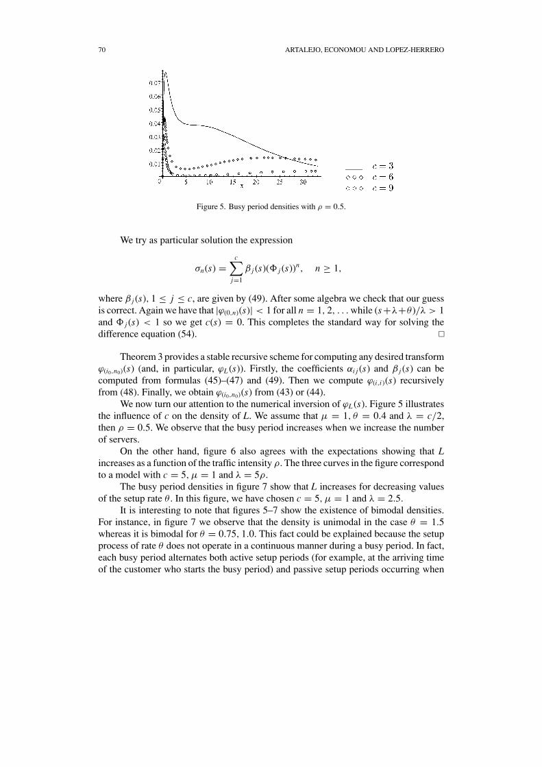
We now turn our attention to the numerical inversion of ϕL (s). Figure 5 illustratesthe influence of c on the density of L. We assume that μ = 1, θ = 0.4 and λ = c/2,then ρ = 0.5. We observe that the busy period increases when we increase the numberof servers.

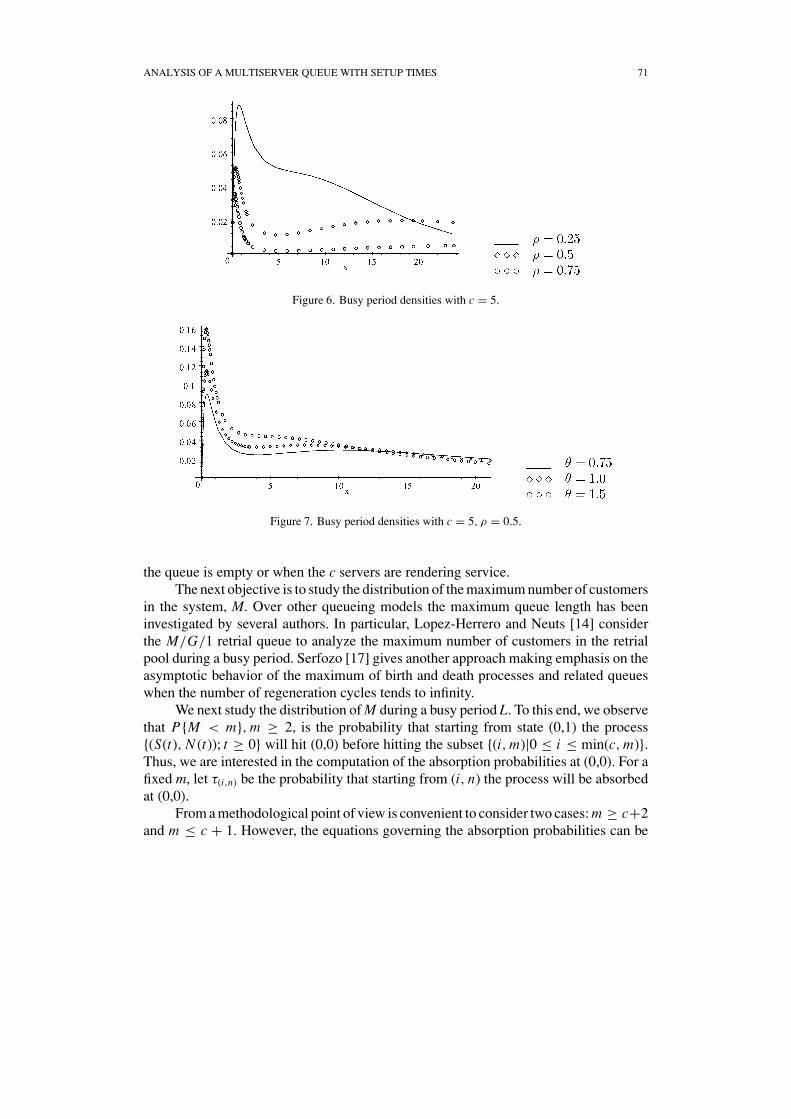
On the other hand, figure 6 also agrees with the expectations showing that Lincreases as a function of the traffic intensity ρ. The three curves in the figure correspondto a model with c = 5, μ = 1 and λ = 5ρ.

The busy period densities in figure 7 show that L increases for decreasing valuesof the setup rate θ . In this figure, we have chosen c = 5, μ = 1 and λ = 2.5.

It is interesting to note that figures 5–7 show the existence of bimodal densities.For instance, in figure 7 we observe that the density is unimodal in the case θ = 1.5whereas it is bimodal for θ = 0.75, 1.0. This fact could be explained because the setupprocess of rate θ does not operate in a continuous manner during a busy period. In fact,each busy period alternates both active setup periods (for example, at the arriving timeof the customer who starts the busy period) and passive setup periods occurring when


Figure 6. Busy period densities with c = 5.

Figure 7. Busy period densities with c = 5, ρ = 0.5.

the queue is empty or when the c servers are rendering service.The next objective is to study the distribution of the maximum number of customers

in the system, M. Over other queueing models the maximum queue length has beeninvestigated by several authors. In particular, Lopez-Herrero and Neuts [14] considerthe M/G/1 retrial queue to analyze the maximum number of customers in the retrialpool during a busy period. Serfozo [17] gives another approach making emphasis on theasymptotic behavior of the maximum of birth and death processes and related queueswhen the number of regeneration cycles tends to infinity.

We next study the distribution of M during a busy period L. To this end, we observethat P{M < m}, m ≥ 2, is the probability that starting from state (0,1) the process{(S(t), N (t)); t ≥ 0} will hit (0,0) before hitting the subset {(i, m)|0 ≤ i ≤ min(c, m)}.Thus, we are interested in the computation of the absorption probabilities at (0,0). For afixed m, let τ(i,n) be the probability that starting from (i, n) the process will be absorbedat (0,0).

From a methodological point of view is convenient to consider two cases: m ≥ c+2and m ≤ c + 1. However, the equations governing the absorption probabilities can be


Figure 8. Mass functions, c = 3, μ = 1, θ = 0.4.

presented under the following unified formulation:

τ(0,0) = 1, (55)

τ(0,n) = λ

λ + θτ(0,n+1) + θ

λ + θτ(1,n), 1 ≤ n ≤ m − 1, (56)

τ(i,i) = λ

λ + iμτ(i,i+1) + iμ

λ + iμτ(i−1,i−1), 1 ≤ i ≤ min(c, m − 1), (57)

τ(i,n) = λ

λ + iμ + θτ(i,n+1) + iμ

λ + iμ + θτ(i,n−1) + θ

λ + iμ + θτ(i+1,n),

1 ≤ i ≤ min(c, m − 1) − 1, i + 1 ≤ n ≤ m − 1, (58)

τ(i,m) = 0, 0 ≤ i ≤ min(c, m). (59)

In addition, in the case m ≥ c+2, the system must be completed with the equation

τ(c,n) = λ

λ + cμτ(c,n+1) + cμ

λ + cμτ(c,n−1), c + 1 ≤ n ≤ m − 1. (60)

Once more the system (55)–(60) can be solved by using the general theory fordifference equations but the algebra becomes now more involved. The solution has beensummarized in Theorem 5 of the Appendix.

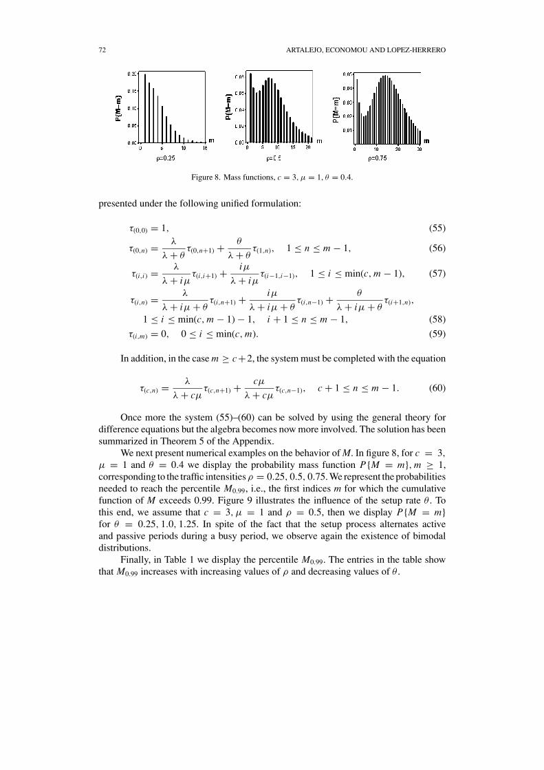
We next present numerical examples on the behavior of M. In figure 8, for c = 3,

μ = 1 and θ = 0.4 we display the probability mass function P{M = m}, m ≥ 1,corresponding to the traffic intensitiesρ = 0.25, 0.5, 0.75. We represent the probabilitiesneeded to reach the percentile M0.99, i.e., the first indices m for which the cumulativefunction of M exceeds 0.99. Figure 9 illustrates the influence of the setup rate θ . Tothis end, we assume that c = 3, μ = 1 and ρ = 0.5, then we display P{M = m}for θ = 0.25, 1.0, 1.25. In spite of the fact that the setup process alternates activeand passive periods during a busy period, we observe again the existence of bimodaldistributions.

Finally, in Table 1 we display the percentile M0.99. The entries in the table showthat M0.99 increases with increasing values of ρ and decreasing values of θ .


Table 199% percentile.

M0.99 θ = 0.1 θ = 0.5 θ = 0.9 θ = 1.3

ρ = 0.1 17 6 5 4ρ = 0.3 47 13 9 8ρ = 0.5 74 21 15 12ρ = 0.7 123 32 23 20ρ = 0.9 176 63 54 50

Figure 9. Mass functions, c = 3, μ = 1, ρ = 0.5.

Appendix

This appendix contains the solutions of the systems of equations (26)–(28) and (55)–(60)which govern respectively the waiting time distribution of a tagged customer, W(i,n), andthe maximum number of customers present in a busy period, M. In particular, we haveP{M = m} = P{M < m+1}−P{M < m}, m ≥ 1, where P{M < m} = τ(0,1), m ≥ 2,and P{M < 1} = 0.

Theorem 4. The Laplace-Stieltjes transforms W (i,n)(s) can be expressed as follows:

W (i,n)(s) =c∑

j=i

αi j (s)( j (s))n−i , 1 ≤ i ≤ c, n ≥ i,

W (0,n)(s) = θ

s + θ

c∑j=1

α1 j (s)( j (s))n−1, n ≥ 1,

where the coefficients αi j (s), 1 ≤ i ≤ j ≤ c, are computed by the reversed recursivescheme

αcc(s) = 1,

αi j (s) = θαi+1, j (s)

(s + iμ + θ ) j (s) − iμ, 1 ≤ i ≤ c − 1, i + 1 ≤ j ≤ c,


αi i (s) = 1 −c∑

j=i+1

αi j (s), 1 ≤ i ≤ c − 1,

and

j (s) = jμs + jμ + θ

, 1 ≤ j ≤ c − 1, c(s) = cμs + cμ

.

Theorem 5. Let us fix the integer m ≥ 2. If m ≥ c + 2, then the probabilities τ(i,n)

satisfy the recursive expressions:

τ(i,n) =(

c∑j=i

αi j ρ jn−i +

c∑j=i

αi j ρ jn−i

)τ(i,i), 1 ≤ i ≤ c, i ≤ n ≤ m,

τ(0,0) = 1,

τ(0,n) =c∑

j=1

β j ρ jn(

1 −(

λρ j

λ + θ

)m−n)+

c∑j=1

β j ρ jn(

1 −(

λρ j

λ + θ

)m−n), 1 ≤ n ≤ m,

where

ρc = 1, ρc = cμλ

> 1,

ρ j = λ + jμ + θ −√

(λ + jμ + θ )2 − 4λ jμ2λ

, 1 ≤ j ≤ c − 1,

ρ j = λ + jμ + θ +√

(λ + jμ + θ )2 − 4λ jμ2λ

, 1 ≤ j ≤ c − 1.

The coefficients αi j and αi j , 1 ≤ i ≤ j ≤ c, are computed by the recursive scheme

αcc = − ρmc

ρcc − ρm

c, αcc = ρc

c

ρcc − ρm

c,

αi j = θ (i + 1)μαi+1, j((λ + iμ + θ )ρ j − λρ2

j − iμ)(

λ + (i + 1)μ − λ�cj=i+1αi+1, j ρ j − λ�c

j=i+1αi+1, j ρ j) ,

αi j = θ(i + 1)μαi+1, j((λ + iμ + θ )ρ j − λρ2

j − iμ)(

λ + (i + 1)μ − λ�cj=i+1αi+1, j ρ j − λ�c

j=i+1αi+1, j ρ j) ,

1 ≤ i ≤ c − 1, i + 1 ≤ j ≤ c,

αi i =(1 − �c

j=i+1αi j − �cj=i+1αi j

)ρm−i

i + (�c

j=i+1αi j ρm−ij + �c

j=i+1αi j ρm−ij

)ρm−i

i − ρm−ii

, 1 ≤ i ≤ c − 1,

αi i = −(1 − �c

j=i+1αi j − �cj=i+1αi j

)ρm−i

i + (�c

j=i+1αi j ρm−ij +�c

j=i+1αi j ρm−ij

)ρm−i

i − ρm−ii

, 1 ≤ i ≤ c−1,

and τ(i,i) is obtained by

τ(0,0) = 1,


τ(i,i) =(

λ + iμ − λ

c∑j=i

αi j ρ j − λ

c∑j=i

αi j ρ j

)−1

iμτ(i−1,i−1), 1 ≤ i ≤ c.

Finally, the coefficients β j and β j are computed by

β j = θμα1 j((λ + θ )ρ j − λρ2

j

)(λ + μ − λ�c

j=1α1 j ρ j − λ�cj=1α1 j ρ j

) , 1 ≤ j ≤ c,

β j = θμα1 j((λ + θ )ρ j − λρ2

j

)(λ + μ − λ�c

j=1α1 j ρ j − λ�cj=1α1 j ρ j

) , 1 ≤ j ≤ c.

On the other hand, for the case m ≤ c + 1, the starting point on the recursivecomputation of the coefficients αi j and αi j is

αm−1,m−1 = − ρm−1

ρm−1 − ρm−1, αm−1,m−1 = ρm−1

ρm−1 − ρm−1.

The rest of coefficients and relationships are analogous to the case m ≥ c + 2 withc replaced by m − 1 in all places.

Acknowledgments

We thank the referees for their constructive comments on an earlier version of the paper.J.R. Artalejo and M.J. Lopez-Herrero thank the support received from DGINV throughthe research project BFM2002-02189. A. Economou was supported by the Universityof Athens grant ELKE/70/4/6415 and by the Greek Ministry of Education and EuropeanUnion Program PYTHAGORAS/2004.

References

[1] I. Adan and J. van der Wal, Combining make to order and make to stock, OR Spektrum 20 (1998)73–81.

[2] I. Adan and J. van der Wal, Difference and Differential Equations in Stochastic Operations Research(1998).

[3] J.R. Artalejo and A. Economou, Markovian controllable queueing systems with hysteretic policies:Analysis of the busy period and the waiting time distributions, Methodology and Computing in AppliedProbability (to appear).

[4] J.R. Artalejo and M.J. Lopez-Herrero, On the M/M/m queue with removable servers, in: StochasticPoint Processes, S.K. Srinivasan and A. Vijayakumar eds. (Narosa Publishing House, 2003) pp. 124–143.

[5] D. Bertsimas, An exact FCFS waiting time analysis for a general class of G/G/s queueing systems,Queueing Systems 3 (1988) 305–320.

[6] W. Bischof, Analysis of M/G/1-queues with setup times and vacations under six different servicedisciplines, Queueing Systems 39 (2001) 265–301.


[7] A. Borthakur and G. Choudhury, A multiserver Poisson queue with a general startup time underN -Policy, Calcutta Statistical Association Bulletin 49 (1999) 199–213.

[8] G. Choudhury, On a batch arrival Poisson queue with a random setup and vacation period, Computersand Operations Research 25 (1998) 1013–1026.

[9] G. Choudhury, An MX/G/1 queueing system with a setup period and a vacation period, QueueingSystems 36 (2000) 23–38.

[10] S.N. Elaydi, An Introduction to Difference Equations, Mathematics. (Springer-Verlag, New York,1999).

[11] Q.M. He and E. Jewkes, Flow time in the MAP/G/1 queue with customer batching and setup times,Stochastic Models 11 (1995) 691–711.

[12] G.V. Krishna Reddy, R. Nadarajan, and R. Arumuganathan, Analysis of a bulk queue with N -policymultiple vacations and setup times, Computers and Operations Research 25 (1998) 957–967.

[13] Y. Levy and U. Yechiali, An M/M/s queue with servers’ vacations, INFOR 14 (1976) 153–163.[14] M.J. Lopez-Herrero and M.F. Neuts, The distribution of the maximum orbit size of an M/G/1 re-

trial queue during the busy period, in: Advances in Stochastic Modelling, eds. J.R. Artalejo and A.Krishnamoorthy (Notable Publications Inc., 2002) pp. 219–231.

[15] M.F. Neuts, Matrix-Geometric Solutions in Stochastic Models: An Algorithmic Approach (JohnsHopkins University Press, Baltimore, 1981, reprinted by Dover Publications, New York, 1994).

[16] J. Resing and R. Rietman, The M/M/1 queue with gated random order of service, Statistica Neer-landica 58 (2004) 97–110.

[17] R.F. Serfozo, Extreme values of birth and death processes and queues, Stochastic Processes and theirApplications 27 (1988) 291–306.

[18] N. Tian, Q.L. Li and J. Cao, Conditional stochastic decompositions in the M/M/c queue with servervacations, Stochastic Models 15 (1999) 367–377.

[19] Z.G. Zhang and N. Tian, Analysis of queueing systems with synchronous single vacation for someservers, Queueing Systems 45 (2003) 161–175.

Analysis of a Multiserver Queue with Setup Times

Documents

Transcript of Analysis of a Multiserver Queue with Setup Times