Transportation Research Part C 17 (2009) 412–427

Contents lists available at ScienceDirect

Transportation Research Part C

journal homepage: www.elsevier .com/locate / t rc

Real-time queue length estimation for congested signalized intersections

Henry X. Liu *, Xinkai Wu 1, Wenteng Ma 1, Heng Hu 1

Department of Civil Engineering, University of Minnesota – Twin Cities, 500 Pillsbury Drive S.E., Minneapolis, MN 55455, United States

a r t i c l e i n f o

Article history:Received 6 November 2008Received in revised form 22 February 2009Accepted 24 February 2009

Keywords:Queue length estimationTraffic signalShockwaveHigh-resolution event-based data

0968-090X/$ - see front matter � 2009 Elsevier Ltddoi:10.1016/j.trc.2009.02.003

* Corresponding author. Tel.: +1 612 625 6347; faE-mail addresses: henryliu@umn.edu (H.X. Liu), w

1 Tel.: +1 612 625 0249; fax: +1 612 625 7750.

a b s t r a c t

How to estimate queue length in real-time at signalized intersection is a long-standingproblem. The problem gets even more difficult when signal links are congested. The tradi-tional input–output approach for queue length estimation can only handle queues that areshorter than the distance between vehicle detector and intersection stop line, becausecumulative vehicle count for arrival traffic is not available once the detector is occupiedby the queue. In this paper, instead of counting arrival traffic flow in the current signalcycle, we solve the problem of measuring intersection queue length by exploiting thequeue discharge process in the immediate past cycle. Using high-resolution ‘‘event-based”traffic signal data, and applying Lighthill–Whitham–Richards (LWR) shockwave theory, weare able to identify traffic state changes that distinguish queue discharge flow fromupstream arrival traffic. Therefore, our approach can estimate time-dependent queuelength even when the signal links are congested with long queues. Variations of the queuelength estimation model are also presented when ‘‘event-based” data is not available. Ourmodels are evaluated by comparing the estimated maximum queue length with the groundtruth data observed from the field. Evaluation results demonstrate that the proposed mod-els can estimate long queues with satisfactory accuracy. Limitations of the proposed modelare also discussed in the paper.

� 2009 Elsevier Ltd. All rights reserved.

1. Introduction

It has long been recognized that vehicular queue length is crucial to either signal performance measures in terms of vehi-cle delay and stops (Webster and Cobbe, 1966; Cronje, 1983a,b; Balke et al., 2005), or signal optimization (Webster, 1958;Gazis, 1964; Newell, 1965; Green, 1968; Michalopoulos and Stephanopolos, 1977a,b; Chang and Lin, 2000; Mirchandani andZou, 2007). Over the years, many researchers have dedicated themselves to this topic and two types of queue estimationmodels have been developed. The first one, which is based on the analysis of cumulative traffic input–output to a signal link,was proposed by Webster (1958) and later improved by a number of researchers (Newell, 1965; Robertson, 1969; Gazis,1974; May, 1975; Catling, 1977; Akcelik, 1999; Strong, et al., 2006; Sharma et al., 2007; Vigos et al., 2008). Such model iscommonly used to describe traffic queuing processes, but ‘‘it is insufficient for obtaining the spatial distribution of queuelengths in time” (Michalopoulos and Stephanopolos, 1981). In addition, cumulative input–output techniques can only beused for the estimation of queue length when the rear of the queue does not exceed the vehicle detector. It cannot handlelong queues exceeding beyond the detector, therefore applications of the technique are limited.

The second model is based on the behavior of traffic shockwaves. The theory was first demonstrated by Lighthill andWhitham (1955) and Richards (1956) for uninterrupted flow; and later expanded by Stephanopolos and Michalopoulos(1979, 1981) to signalized intersections. Essentially, this model estimates queue lengths by tracing the trajectory of

. All rights reserved.

x: +1 612 625 7750.uxxx273@umn.edu (X. Wu), maxxx130@umn.edu (W. Ma), huxxx186@umn.edu (H. Hu).

H.X. Liu et al. / Transportation Research Part C 17 (2009) 412–427 413

shockwaves based on the continuum traffic flow theory. Although shockwave theory successfully describes the complexqueuing process in both temporal and spatial dimensions, these elegant theoretical models have limitations in the practicalapplications as they require ‘‘perfect” input information. In other words, these models assume known vehicle arrivals, whichcannot be satisfied for most of situations. Vehicle arrivals cannot be measured when detector is occupied, which is usually thecase with congested arterials. Without arrival information, existing shockwave models cannot be utilized to estimate inter-section queue lengths.

To estimate the queue length longer than the distance from intersection stop bar to advance detector, Muck (2002) ex-plored the relationship between the ‘‘fill-up” time, i.e., the time ‘‘passes from the beginning of the red time of a signal untilcontinuous occupancy of a detector”, and queue sizes, using a linear regression model. The evaluation result shows that thismethod can estimate queues up to 5–10 times further upstream from the actual detector location. However, Muck’s heuristicapproach is based upon the premise that arrival rate of traffic flow is constant within a cycle; therefore the measured fill-uptime can be proportionally inverse to the queue build-up speed. Such an approach could be problematic when arrival rate oftraffic flow fluctuate greatly, which is not unusual with the ‘‘gating effect” of an upstream traffic signal.

Skabardonis and Geroliminis (2008) proposed a method to estimate intersection queue length using aggregated loopdetector data in 30-s intervals. In their method, they examine the flow and occupancy changes from the loop detector datato determine the queue rear end. The problem is that since 30-s aggregation smoothes out variations for between-vehiclegaps, it is difficult to identify the queue rear unless the arrival traffic flow is significant different with the queue dischargeflow. In addition, since queue length estimation is only part of their travel time estimation model, no evaluation results arereported in their paper to verify the accuracy of the queue length estimation method.

It is the objective of this paper to provide a method for estimation of long queues (meaning ‘‘longer than the distancebetween intersection stop line to location of vehicle detectors”). We are particularly interested in the estimation of maxi-mum queue length, i.e., the distance from the intersection stop line to the position of the last vehicle that has to stop in acycle. The proposed methodology relies on high resolution traffic signal data, which becomes increasingly available in recentyears. For example, second-by-second detector data has been used by ACS-Lite (Adaptive Control Software Lite) (Luyanda,et al., 2003). Event-based data (including both vehicle-detector actuation events and signal phase change events) can beautomatically collected archived by the SMART–SIGNAL system (Systematic Monitoring of Arterial Road Traffic and Signals)developed at the University of Minnesota (Liu and Ma, 2008, 2009). Such high resolution data, to some extent, can be utilizedto recover the event history of a traffic signal and provide us the basis to analyze the relationship between signal phasechanges and traffic flow during the queue forming and discharging processes. In particular, such high resolution data revealssome ‘‘break points” that identify traffic flow pattern changes, which have important physical meaning in terms of trafficshockwave and contribute significantly to the long queue estimation. We will demonstrate that by applying simple shock-wave theory originally developed by Lighthill and Whitham (1955) and Richards (1956) with such data, intersection queuelength can be accurately estimated using existing detectors.

It should be also note that our queue length estimation methods will work with typical detector configurations for signaloperation, i.e., with either stopbar detector for vehicle presence detection or advance detector (a few hundred feet upstreamfrom stopline) for green extension, or both. We do not assume a link input detector, i.e., a detector placed sufficiently up-stream so that input traffic flow to the traffic signal can be measured, subsequently input–output approach can be utilizedfor queue estimation. Such detector, however, is usually not available in the real-world.

This paper is organized as following. The shockwave theory is reviewed in Section 2, followed by data description and‘‘break points” identification. The analytical model is presented in Section 3, as well as two expansion models that allow vari-ations of high-resolution traffic signal data can be used for specific real world scenarios. The testing results are shown inSection 4 followed by discussion and conclusions.

2. Shock wave analysis and ‘‘break points identification

2.1. Shock wave analysis

The traditional Lighthill–Whitham–Richards (LWR) traffic flow model hypothesizes that flow is a function of density atany point of the road. A shockwave is defined as ‘‘the motion (or propagation) of an abrupt change (discontinuity) in con-centration” (Stephanopolos and Michalopoulos, 1979). Traffic shockwave theory is derived from LWR model when applyingthe method of characteristics to analytically solve the partial differential equation (PDE) in the model. Basically, when char-acteristic curves (along which, the density is constant) interact, a shockwave is formed and wave velocity can be determinedby following equation (Eq. (1))

uw ¼DqDk¼ q2 � q1

k2 � k1¼ k2u2 � k1u1

k2 � k1ð1Þ

where q1, k1, u1 are the flow, density and velocity of the upstream region and q2, k2, u2 are the flow, density and velocity ofthe downstream region. Traffic shockwave can be also illustrated by using the fundamental diagram (q–k curve). The tangentof the chord drawn between any two points on the q–k curve defines the shockwave speed, as shown in Fig. 1 (we will ex-plain v1, v2, and v3 in the following).

Fundamental Diagram

maxq

maxk

( )aa kq ,

( )mm kq ,

( )jk,0

jk

2v

1v

Flow

Density

3v

Fig. 1. Representation of shockwaves in the fundamental diagram.

414 H.X. Liu et al. / Transportation Research Part C 17 (2009) 412–427

At signalized intersections, multiple shock waves are generated due to the stop-and-go traffic caused by signal changes.For better explanation simply assume that queue has been fully discharged during the last green phase. In the following redinterval, vehicles are forced to stop, which creates different flow and density conditions between the arrival and the stoppedtraffic. Such interruption of traffic flow, as indicated in Fig. 2a, forms a queuing shockwave v1 in Fig. 1 moving upstream ofthe intersection with velocity

v1 ¼0� qn

a

kj � kna

ð2Þ

where 0 and kj represent the jammed flow and density; and qna and kn

a are the average arrival flow rates and density duringthe nth cycle (subscript a means ‘‘arrival traffic”). In Fig. 2, Tn

g and Tnr indicate the end time and the start time of the effective

green, respectively, during the nth cycle.The queuing shockwave v1 keeps propagating to upstream. At the beginning of the effective green (Tn

r in Fig. 2b), vehiclesbegin to discharge at saturation flow rate (assume there is no congestion downstream) forming the second shock wavewhich is defined as discharge shockwave v2 in Fig. 2 at the stop line moving upstream with speed

v2 ¼qm � 0km � kj

ð3Þ

where qm and km are the capacity or saturation flow and density.The discharge shockwave m2 usually has higher speed than v1, so the two waves will meet at time Tn

max (in Fig. 2c), which isthe time that this approach has the maximum queue length. As soon as the two shock waves meet, a third one (defined as adeparture shockwave, v3 in Fig. 1) is generated propagating toward the stop line with speed

v3 ¼qm � qn

a

km � kna

ð4Þ

At the end of this cycle, i.e., the start of the red phase of the next cycle, if the queue cannot be fully discharged, a residualqueue is formed, which builds the fourth shock wave v4 (Fig. 2d) at stop line moving upstream with speed

v4 ¼0� qm

kj � kmð5Þ

Shock wave v4 describes the queue compression process. Waves v3 and v4 have inverse directions therefore they meet attime Tn

min (Fig. 2e), which is the time the approach has minimum queue length, i.e., the residual queue. As soon as the twowaves meet the fifth wave v5, which is the new queuing wave of the (n + 1)th cycle, is formed moving upstream with similarspeed as the shock wave v1.

v5 ¼0� qnþ1

a

kj � knþ1a

ð6Þ

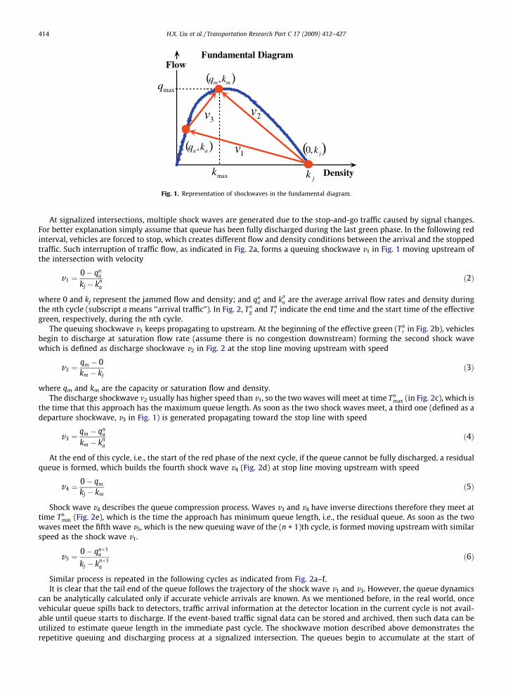
Similar process is repeated in the following cycles as indicated from Fig. 2a–f.It is clear that the tail end of the queue follows the trajectory of the shock wave v1 and v3. However, the queue dynamics

can be analytically calculated only if accurate vehicle arrivals are known. As we mentioned before, in the real world, oncevehicular queue spills back to detectors, traffic arrival information at the detector location in the current cycle is not avail-able until queue starts to discharge. If the event-based traffic signal data can be stored and archived, then such data can beutilized to estimate queue length in the immediate past cycle. The shockwave motion described above demonstrates therepetitive queuing and discharging process at a signalized intersection. The queues begin to accumulate at the start of

a

c

b

d

fe

Fig. 2. Shock wave propagation.

H.X. Liu et al. / Transportation Research Part C 17 (2009) 412–427 415

red interval and discharge at the beginning of green phase. Sometime after the green start, maximum queue length isachieved; and shortly after the red start, minimum queue length (i.e., residual queue) is formed. Such repeated process givesus some hints that if some crucial ‘‘break points” can be identified utilizing detector data, then the queuing and discharging

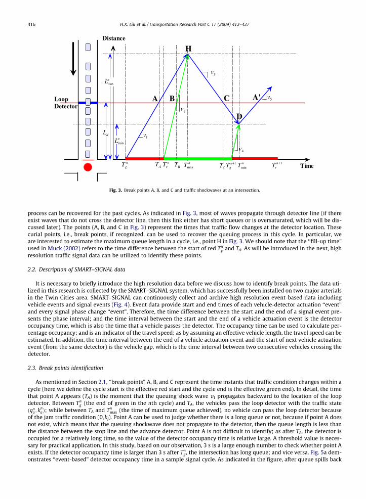
Fig. 3. Break points A, B, and C and traffic shockwaves at an intersection.

416 H.X. Liu et al. / Transportation Research Part C 17 (2009) 412–427

process can be recovered for the past cycles. As indicated in Fig. 3, most of waves propagate through detector line (if thereexist waves that do not cross the detector line, then this link either has short queues or is oversaturated, which will be dis-cussed later). The points (A, B, and C in Fig. 3) represent the times that traffic flow changes at the detector location. Thesecurial points, i.e., break points, if recognized, can be used to recover the queuing process in this cycle. In particular, weare interested to estimate the maximum queue length in a cycle, i.e., point H in Fig. 3. We should note that the ‘‘fill-up time”used in Muck (2002) refers to the time difference between the start of red Tn

g and TA. As will be introduced in the next, highresolution traffic signal data can be utilized to identify these points.

2.2. Description of SMART–SIGNAL data

It is necessary to briefly introduce the high resolution data before we discuss how to identify break points. The data uti-lized in this research is collected by the SMART–SIGNAL system, which has successfully been installed on two major arterialsin the Twin Cities area. SMART–SIGNAL can continuously collect and archive high resolution event-based data includingvehicle events and signal events (Fig. 4). Event data provide start and end times of each vehicle-detector actuation ‘‘event”and every signal phase change ‘‘event”. Therefore, the time difference between the start and the end of a signal event pre-sents the phase interval; and the time interval between the start and the end of a vehicle actuation event is the detectoroccupancy time, which is also the time that a vehicle passes the detector. The occupancy time can be used to calculate per-centage occupancy; and is an indicator of the travel speed; as by assuming an effective vehicle length, the travel speed can beestimated. In addition, the time interval between the end of a vehicle actuation event and the start of next vehicle actuationevent (from the same detector) is the vehicle gap, which is the time interval between two consecutive vehicles crossing thedetector.

2.3. Break points identification

As mentioned in Section 2.1, ‘‘break points” A, B, and C represent the time instants that traffic condition changes within acycle (here we define the cycle start is the effective red start and the cycle end is the effective green end). In detail, the timethat point A appears (TA) is the moment that the queuing shock wave v1 propagates backward to the location of the loopdetector. Between Tn

g (the end of green in the nth cycle) and TA, the vehicles pass the loop detector with the traffic stateðqn

a ; knaÞ; while between TA and Tn

max (the time of maximum queue achieved), no vehicle can pass the loop detector becauseof the jam traffic condition (0,kj). Point A can be used to judge whether there is a long queue or not, because if point A doesnot exist, which means that the queuing shockwave does not propagate to the detector, then the queue length is less thanthe distance between the stop line and the advance detector. Point A is not difficult to identify; as after TA, the detector isoccupied for a relatively long time, so the value of the detector occupancy time is relative large. A threshold value is neces-sary for practical application. In this study, based on our observation, 3 s is a large enough number to check whether point Aexists. If the detector occupancy time is larger than 3 s after Tn

g , the intersection has long queue; and vice versa. Fig. 5a dem-onstrates ‘‘event-based” detector occupancy time in a sample signal cycle. As indicated in the figure, after queue spills back

Fig. 4. Sample data collected at the intersection.

Case 1 - Long Queue

0

10

20

30

40

50

7:26:07 7:26:50 7:27:33 7:28:16 7:29:00

Case 1 - Long Queue

0

2.5

5

7.5

10

7:26:07 7:26:50 7:27:33 7:28:16 7:29:00

Detector Occupancy Time

Break Point A Break Point B

Time Gap Between Consecutive Vehicles

),( mm kq

),( na

na kq

Pattern I: Capacity condition

Pattern II: Free flow arrival

Break Point C

(Sec)

(Sec)

Time

Time

a

b

Fig. 5. (a) Detector occupancy profile in a cycle; (b) time gap between consecutive vehicles in a cycle.

H.X. Liu et al. / Transportation Research Part C 17 (2009) 412–427 417

to the advance detector, the occupancy time is significantly larger than 3 s (about 45 s in this particular cycle). We shouldpoint out that second-by-second percentage occupancy data can also be utilized to identify point A, i.e., the occupancy valueis kept at 100% for more than 3 s.

Point B indicates the time (TB) that the discharge shockwave passes the detector. Between effective green start ðTnr Þ and, TB

the traffic state over the detector is (0,kj); after TB, vehicles are discharged at saturation flow rate and traffic state changes to(qm,km). It is also not difficult to identify Point B using high resolution data. After the green starts and before TB, traffic volumeis zero, and detector occupancy time is high (larger than 3 s) or second-by-second percentage occupancy continues to be 100%for at least 3 s. After TB, queued vehicles begin to discharge over the detector, therefore both detector occupancy time and timegap between consecutive vehicles drop. As indicated in Fig. 5a, the detector occupancy time drops significantly after TB.

The most important break point is point C. As will be introduced in the next section, the time of point C (TC), combinedwith the discharge shock wave v2, will be utilized to estimate the maximum queue length and re-construct queue formingand discharging process. Point C indicates the time (TC) when the rear end of queue passes the detector. The time duration

418 H.X. Liu et al. / Transportation Research Part C 17 (2009) 412–427

between TB and TC is closely related to the estimation of maximum queue length. As introduced before, wave v3 is the inter-face between saturation traffic state (qm,km) and the arrival traffic state ðqn

a ; knaÞ. Therefore, before point C appears, vehicles

discharge at the saturation flow rate at the location of loop detector, i.e., the traffic state is (qm,km). After the wave propagatesto the detector location, the traffic condition becomes to ðqn

a ; knaÞ, i.e., the discharge rate at the loop detector location is less

than saturation flow. A threshold should be selected to identify the two different traffic states (qm,km) and ðqna ; k

naÞ. Based on

our observation, the time gap between two consecutive vehicles is sensitive to traffic state change. As indicated in Fig. 5b,traffic is separated into two states by break point C. Before TC, the time gaps between vehicles are small (less than 2.5 s) andthe variance is small. It means that most of vehicles are discharged at saturation flow rate. But after TC, the vehicle gaps be-come much bigger and the variance is significantly increased. More importantly, there usually exists a time lag between thesaturated queue discharge flow and newly arrival traffic, as shown in Fig. 5b.

Ideally, statistical analysis of vehicle gap data (for example, comparing the means and variances of time gaps of two vehi-cle groups) is necessary in order to recognize traffic state change. However, for simplicity and practicality, a threshold valuefor the time lag between saturated queue discharge flow and arrival traffic is determined based on our observation. In thisstudy, if the value of time gap is larger than 2.5 s, we consider that the end of queue is propagated forward and has reachedthe detector line, therefore TC is identified. Considering the variation of time gaps, using a single value to separate trafficstates may bring large error. In our implementation, if the time gap is between 2.5 s and 3 s, the system will continue search-ing the second and third points with time gaps over 2.5 s to make sure that the traffic state is really changed. It should be alsonoted that if only second-by-second data is available, the method described above is still feasible. As we know that largerthan 2.5 s gap means 0% occupancy for at least two consecutive seconds.

Two other interesting cases are demonstrated in Fig. 6, one is that the break point C cannot be found; and the other is thatvehicles arrive as a platoon. In Fig. 6a, during the green phase, the traffic pattern does not change and vehicles keep discharg-ing at saturation flow rate. This case could be caused by two reasons: (1) vehicle queue cannot be discharged completely andthis approach at this cycle is possibly oversaturated; (2) vehicle platoon arrives within a small time lag so that a large vehiclegap cannot be found. The other case, as indicated in Fig. 6b, is that although the break point is easy to find, the traffic patternbefore and after break point, however, is similar. The explanation of this situation is that after the queue has been discharged,a platoon discharged from upstream intersection arrives. This situation, sometimes, will bring error to our queue estimationmodel, which will be discussed in the later sections.

3. Queue estimation models

The models proposed here are to utilize the break points (A, B and C) identified in the last section using high resolutiondata. As indicated in Fig. 3, the crucial part is how to estimate the coordinate of point H, the maximum queue, in both spatial(i.e., queue length) and temporal ðTn

maxÞ dimensions. Point H is the intersection point of three waves and its coordinate can bedecided by any two of them. As mentioned above, wave v1 is a queuing wave, which highly depends on traffic arrival.Although wave v3 is also related to arrival flow (Eq. (4)), it is the arrival traffic after queue discharge so that the traffic statecan be estimated using detector data. Therefore, in this research, wave v2, which has a constant velocity (as shown in Eq. (3)if we assume saturation flow rate ðqmÞ, saturation density ðkmÞ, and jam density ðkjÞ, are known a priori), and wave v3 areutilized to identify the coordinate of point H, i.e., the location and time when maximum queue is reached. One basic modeland two expansions, which are specially designed for some practical applications, are discussed in this section.

3.1. Basic model

To estimate shockwave speeds, v2 and v3, we need to ‘‘mine” more information from high resolution event-based datafrom one single loop detector. Shockwave speed v2 can be estimated using the distance between advance detector and stop-bar (Ld) and the time difference between the green start ðTn

r Þ and the time discharge wave reaching advance detector (TB), i.e.,v2 ¼ Ld=ðTB � Tn

r Þ. Shockwave speed v2 can also estimated using Eq. (2) with assumed saturation flow rate (qm), saturationdensity (km), and jam density (kj).

To estimate shockwave speed v3, we will need to estimate two traffic states (qm,km) and ðqna ; k

naÞ and apply Eq. (4). This is

feasible because event-based data record both the occupancy time and the gap between consecutive vehicles passing theloop detector. Occupancy time recorded by detectors can be used to estimate the individual speed by assuming an effectivevehicle length; and the sum of occupancy time and vehicle gap, i.e., headway, can be utilized to estimate the average flow.Then density can be estimated by average flow and space mean speed. Eq. (7) is used to estimate the space mean speed (us),flow (q) and density (k)

ui ¼ Le=to;i

us ¼ 1= 1n

Pni¼1

1ui

� �

q ¼ 1= 1n

Pni¼1

hi

� �¼ 1= 1

n

Pni¼1ðto;i þ tg;iÞ

� �k ¼ q=us

8>>>>>>>><>>>>>>>>:

ð7Þ

0

10

20

30

40

50

7:29:06 7:29:50 7:30:33 7:31:16 7:31:59

0

2.5

5

7.5

10

7:29:06 7:29:50 7:30:33 7:31:16 7:31:59

Detector Occupancy Time

BBrreeaakk PPooiinntt AA BBrreeaakk PPooiinntt BB

Time Gap Between Consecutive Vehicles(Sec)

(Sec)

Time

Time

No pattern changes, always dischargeaatt ssaattuurraattiioonn fffff ooww rraattee

0

5

10

15

20

7:32:07 7:32:50 7:33:33 7:34:17 7:35:00

0

2.5

5

7.5

10

7:32:07 7:32:50 7:33:33 7:34:17 7:35:00

Detector Occupancy Time

BBrreeaakk PPooiiiinnntt AA BBrreeaakk PPooiinntt BB

Time Gap Between Consecutive Vehicles

),( mm kmmqmm

),( na

na kq

Pattern I: Capaccity ccoondition

Pattern II: Freee ff ow aarrival

Break Poinnt CC

(Sec)

(Sec)

Time

Time

a

b

l

l

Fig. 6. Two other cases – (a) oversaturation; (b) platoon arrival.

H.X. Liu et al. / Transportation Research Part C 17 (2009) 412–427 419

where, to,i and tg,i are the detector occupancy time and time gap of vehicle i, respectively; ui,hi are the speed and headway ofvehicle i, respectively; Le is the effective vehicle length, i.e., the sum of average vehicle length and detector length, which mayrequire calibration; and n is the number of vehicles which has been identified with same traffic state.

Distance

Time

1v

2v

ngT n

rT nTmax1+n

gT

3v

nTmin

5v

1+nrT

4v

A B CLoopDetector

H

AT BTCT

dL

nLmax

D

nLmin

1v

A'

Fig. 7. Model I – basic model.

420 H.X. Liu et al. / Transportation Research Part C 17 (2009) 412–427

As we discussed before, the traffic state is (qm,km) between TB and TC, and ðqna ; k

naÞ after TC (and before Tnþ1

g ). Eq. (7) can thenbe applied to estimate these two conditions. Note that in the algorithm, we use observed data to estimate traffic state (qm,km)instead of assuming the constant values; this is because the capacity or saturation flow rate will decrease if the traffic is af-fected by the downstream intersections. The velocity of wave v3 is calculated based on the two estimated traffic conditions.Using estimated m3 and v2, the maximum queue length Ln

max and time Tnmax during nth cycle can be calculated:

Lnmax ¼ Ld þ ðTC � TBÞ 1

v2þ 1

v3

� �.Tn

max ¼ TB þ ðLnmax � LdÞ=v2

8<: ð8Þ

where Ld is the distance from stop line to the loop detector.The minimum queue length Ln

min and time Tnmin (if residual queue exists) during nth cycle can be also calculated:

Lnmin ¼

Lnmaxv3þ Tn

max � Tnþ1g

� �1v3þ 1

v4

� �.Tn

max ¼ Tnþ1g þ Ln

min=v4

8<: ð9Þ

where v4 is the velocity of the shock wave v4, which has similar value as velocity of the shock wave v2 (Eq. (5)).The dynamic queue discharging process after Tn

max (before Tnmin) is easy to be formulated as we know the wave speed v3;

and the queuing process before TA has been recorded by loop detectors (as we can see in Fig. 7, the arrival may not beconstant).

The problem now is to estimate the queue state between points A and H. Without any other information, we can assume aconstant velocity for wave v1, which can be estimated by

v1 ¼ ðLnmax � LdÞ=ðTn

max � TAÞ ð10Þ

Then the entire queue accumulation and discharge processes can be fully described.

3.2. Expansion I – using second-by-second detector data

In the basic model, event-based data is required in order to identify the shockwave speeds; such requirement may not besatisfied in the real world. If second-by-second detector data and signal phase data are available (such as the ACS-Lite sys-tem), the basic model for the calculation of maximum and minimum queue lengths can still be applied by identifying breakpoints A, B and C and calculating traffic state variables using Eq. (7). Model Expansion I provides a simple alternative to cal-culate maximum and minimum queue length, without applying Eq. (7), as explained below.

As we know, among all the vehicles passing loop detectors before TC, most of them are part of the maximum queue Lnmax,

while a small portion of vehicles join the queue after the tail end of original maximum queue began to move. This small por-tion of vehicles theoretically has no contribution to the maximum queue length, but they are affected by the queue. There-

Distance

Time

2v

ngT n

rT ′nTmax

1+ngT

3v

′nTmin

5v

1+nrT

4v

A B C A'LoopDetector

H

AT BTCT

dL

′nLmax

1v

H'

D

D'

1v′3v′

′nLmin

5v′

Fig. 8. Expansion I.

H.X. Liu et al. / Transportation Research Part C 17 (2009) 412–427 421

fore, an approximation can be made to treat all the vehicles passing the detector between the green start and TC as thequeued vehicles. Because the number of vehicles can be easily obtained using second-by-second detector data, by assuminga constant jam density, the maximum queue length ðLn0

maxÞ and the time ðTn0

maxÞ as well as wave speed v 03 under such approx-imation can be directly estimated:

Ln0

max ¼ n=kj þ Ld

Tn0

max ¼ Tnr þ Ln0

max=v2

v 03 ¼ Ln0

max � Ld= TC � Tn0

max

� �8>><>>: ð11Þ

where n is the number of vehicles passing detector between Tng and TC.

By using a constant shock wave speed v4, Eq. (9) can then be applied to estimate the minimum queue length (Ln0

min) and thetime (Tn0

min) as well as wave speed v 01.Essentially, Expansion I is a simplified queue estimation model. As demonstrated in Fig. 8, point H represents the true

maximum queue, while H0 is an approximation. Theoretically, the expanded model I overestimates the maximum queuelength as it includes some portion of vehicles which do not belong to the stopped vehicle queue.

3.3. Expansion II – dealing with wired-together detectors

The expanded model II is specifically designed to deal with a case that detectors in different lanes (in a same approach)are wired together, or a single detector cover multiple lanes. In this case, vehicles traveling at different lanes will be countedonly once if they pass the detector at the same time. This detector configuration is common for many signalized intersectionsin Minnesota. Under such design, although the break points can still be identified by using second-by-second detector data,the vehicle counts are not accurate any more (which means that the Basic Model and Expansion I will not work). An approx-imation is made here to deal with this problem. This approximation is based on the assumption that after the tail end ofmaximum queue begins to move, no additional vehicles can join the queue. Then the shock wave v 003 actually is the trajectoryof the last vehicle. By assuming a priori known constant acceleration speed (3.5 feet/s, for example), the trajectory of thelasted stopped vehicle can be analytically derived.

Depending on whether the last vehicle in the queue reaches maximum speed at point C, the time interval between Tn00

max

and TC (t) in Fig. 9) can be estimated using following equation:

12 a uf

a

� �2 þ uf t � uf

a

� �¼ v2ðTC � TB � tÞ if t P uf

a12 at2 ¼ v2ðTC � tÞ if t < uf

a

(ð12Þ

where uf and a are free flow speed and acceleration speed, respectively.

Distance

Time

2v

ngT n

rT″nTmax

1+ngT

3v

″nTmin

5v

1+nrT

4v

A B C A'LoopDetector

H

AT BTCT

dL

″nLmax1v

H''

D

D''

1v ′′3v ′′

″nLmin t

5v ′′

t

Fig. 9. Expansion II.

422 H.X. Liu et al. / Transportation Research Part C 17 (2009) 412–427

Then the maximum queue length ðLn00

maxÞ and the time ðTn00

maxÞ can be estimated by:

Ln00

max ¼ Ld þ v2ðTC � TB � tÞTn00

max ¼ TC � t

(ð13Þ

Similar formulations are used to estimate the minimum queue length ðLn00

minÞ and the time ðTn00

minÞ as well as wave speed v 001.Clearly, the assumption made in this model may not be true in reality. So for some situation, similar as Expansion I,

Expansion II overestimates the maximum queue. As indicated in Fig. 9, point H is the real maximum queue length, and esti-mated maximum queue length (H00) actually is an overestimation.

4. Implementation

4.1. Implementation procedure

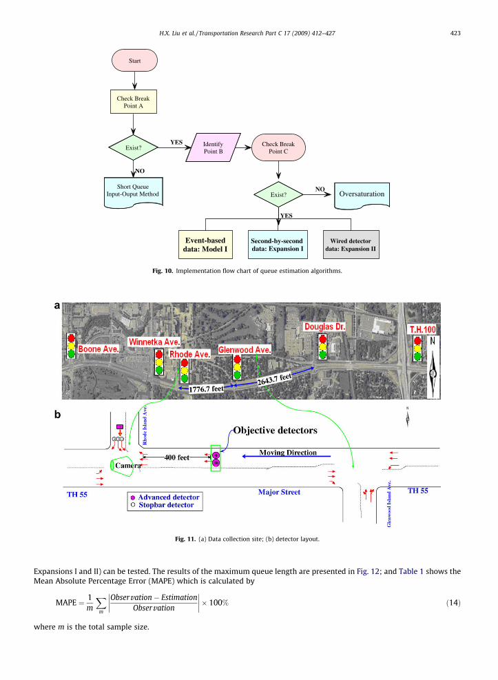
Fig. 10 demonstrates the implementation procedure for the queue length estimation algorithms. To implement such algo-rithms, the first step is to check whether break point A exists. If point A cannot be found, it is a short queue case; and a simpleinput–output method can be applied to estimate queue size. This simple method records number of vehicles passing loopdetector, assumes saturation flow rate discharging when signal turns green, and calculates the residual number of vehicleswithin the area between stop line and the location of the advance detectors. Then queue length can be estimated by simplyassuming an effective vehicle length in jam traffic state. If point A exists, then it requires identifying point B and C. (actually,point B is not necessary to identify because the wave speed v2 for most of situation is a constant value). If point C can beidentified, depending on the resolution of detector data, different models are applied to estimate the long queue. If pointC cannot be identified, as we discussed in the last section, the approach is under oversaturation. The queue length underoversaturated condition is difficult to estimate, but it is longer than or equal to the distance that occupied by the maximumdischargeable queue during green time.

4.2. Field evaluation results by the research team

The intersection of Trunk Highway 55 and Rhode Ave in Minnesota is selected as the testing site because of the frequentoccurrences of extended queues on the west bound (From Glenwood Ave. to Rhode Ave.) during morning peak. Fig. 11a is amap of the intersection (including six coordinated intersections on Trunk Highway 55) and Fig. 11b shows the detector lay-out of the intersection. The data collected from detector #9 and #10 during two morning peak hours with fixed cycle-length(180 s) on June 11th, 2008 (Wednesday) are used to estimate the queue length; and the estimated values are comparedwith the ground truth data, which is recorded by a camera installed at the intersection (the maximum queue length for eachcycle is manually extracted by watching the video). As event-based data are collected by detectors, all three models (basic,

Check BreakPoint A

Exist?

Short QueueInput-Ouput Method

IdentifyPoint B

Check BreakPoint C

Start

NO

YES

Exist?

YES

NOOversaturation

Wired detectordata: Expansion II

Event-baseddata: Model I

Second-by-seconddata: Expansion I

Fig. 10. Implementation flow chart of queue estimation algorithms.

Fig. 11. (a) Data collection site; (b) detector layout.

H.X. Liu et al. / Transportation Research Part C 17 (2009) 412–427 423

Expansions I and II) can be tested. The results of the maximum queue length are presented in Fig. 12; and Table 1 shows theMean Absolute Percentage Error (MAPE) which is calculated by

MAPE ¼ 1m

Xm

Observation� EstimationObservation

��������� 100% ð14Þ

where m is the total sample size.

Maximum Queue Length Comparion - Left Lane

Maximum Queue Length Comparion - Right Lane

Distance (ft)

Distance (ft)

Time

Time

Fig. 12. Testing results.

Table 1MAPE of three models.

MAPE of maximum queue length Basic model (%) Expansion I (%) Expansion II (%)

Left lane (Detector #10) 6.5 15.9 22.3Right lane (Detector #9) 8.7 13.4 18.8

Expansion IExpansion II

Basic Model

Queue Trajectories of Detector #9Distance (ft)

Time

Fig. 13. Queue trajectory.

424 H.X. Liu et al. / Transportation Research Part C 17 (2009) 412–427

As presented in Fig. 12, for both left lane and right lane, the basic model can successfully estimate the maximum queuelength; and the average MAPE is around 7% (Table 1). However, Expansion I and Expansion II, as we mentioned before, over-estimate the maximum queue; and the average absolute percentage errors are about 14% and 20%. Fig. 13 visually presentsthe estimated queue dynamics. It is very clear that the proposed models successfully describe queue forming and discharg-ing processes. In addition, Table 2 presents the time differences when the maximum queue length is reached ðTn00

maxÞ, usingthe three proposed models and real-world observations. The absolute errors for three models are around 5 s.

Table 2Absolute errors of time of maximum queue length.

Absolute errors of time of maximum queue length Basic model (s) Expansion I (s) Expansion II (s)

Left lane (Detector #10) 6 6 5Right lane (Detector #9) 5 6 4

H.X. Liu et al. / Transportation Research Part C 17 (2009) 412–427 425

4.3. Independent evaluation results by Alliant Engineering Inc.

A Minneapolis-based Transportation Consulting firm, Alliant Engineering Inc. also conducted an independent evaluationof the queue length estimation algorithm. To observe the queue length, Alliant sent observers to the field (the Rhode Islandintersection) during morning peak (7:00–9:00 a.m.) on three randomly selected days in 2008: July 23rd, October 29th, andDecember 10th. These observers manually count the vehicles as they enter the queue (they were instructed to count astopped vehicle as one that was traveling at less than 5 miles per hour) and record the time when queue is maximal.

Maximum Queue Length Comparison - Jul. 23rd, 2008

Maximum Queue Length Comparison - Occ. 29th, 2008

Maximum Queue Length Comparison - Dec. 10th, 2008

Distance (ft)

Distance (ft)

Distance (ft)

Time

Time

Time

Observation

Basic Model

Observation

Basic Model

Observation

Basic Model

Fig. 14. Comparison of maximum queue length.

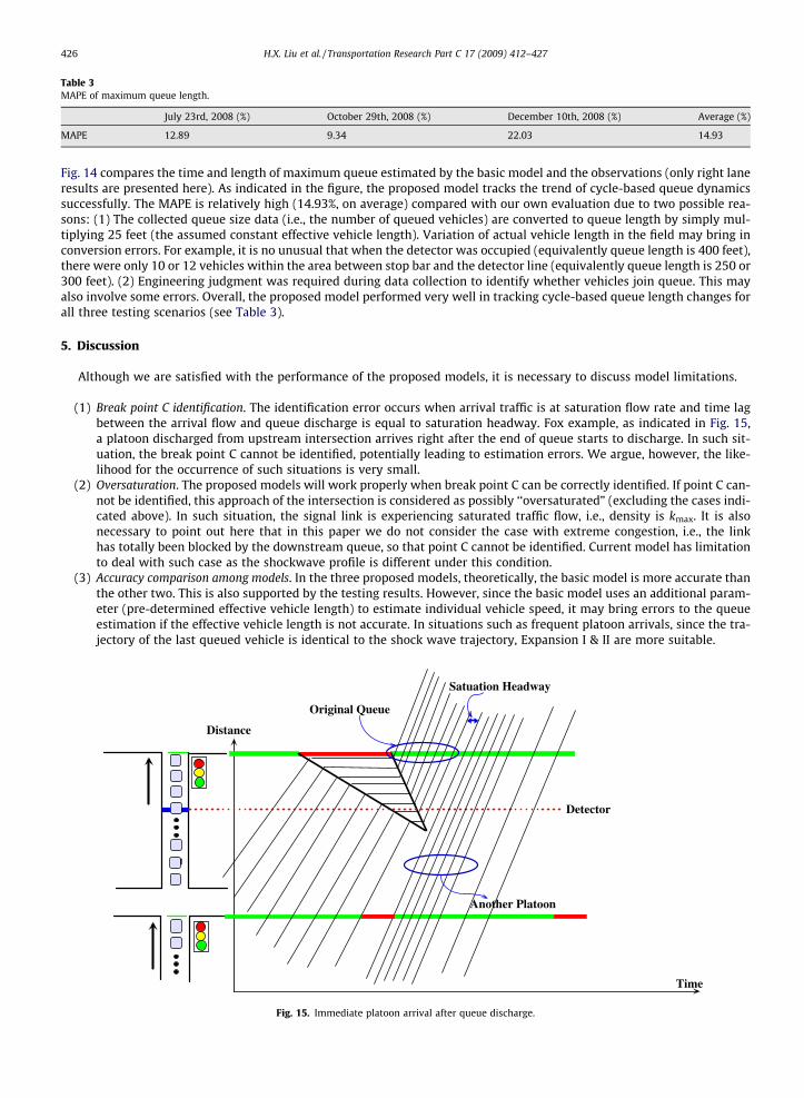
Table 3MAPE of maximum queue length.

July 23rd, 2008 (%) October 29th, 2008 (%) December 10th, 2008 (%) Average (%)

MAPE 12.89 9.34 22.03 14.93

426 H.X. Liu et al. / Transportation Research Part C 17 (2009) 412–427

Fig. 14 compares the time and length of maximum queue estimated by the basic model and the observations (only right laneresults are presented here). As indicated in the figure, the proposed model tracks the trend of cycle-based queue dynamicssuccessfully. The MAPE is relatively high (14.93%, on average) compared with our own evaluation due to two possible rea-sons: (1) The collected queue size data (i.e., the number of queued vehicles) are converted to queue length by simply mul-tiplying 25 feet (the assumed constant effective vehicle length). Variation of actual vehicle length in the field may bring inconversion errors. For example, it is no unusual that when the detector was occupied (equivalently queue length is 400 feet),there were only 10 or 12 vehicles within the area between stop bar and the detector line (equivalently queue length is 250 or300 feet). (2) Engineering judgment was required during data collection to identify whether vehicles join queue. This mayalso involve some errors. Overall, the proposed model performed very well in tracking cycle-based queue length changes forall three testing scenarios (see Table 3).

5. Discussion

Although we are satisfied with the performance of the proposed models, it is necessary to discuss model limitations.

(1) Break point C identification. The identification error occurs when arrival traffic is at saturation flow rate and time lagbetween the arrival flow and queue discharge is equal to saturation headway. Fox example, as indicated in Fig. 15,a platoon discharged from upstream intersection arrives right after the end of queue starts to discharge. In such sit-uation, the break point C cannot be identified, potentially leading to estimation errors. We argue, however, the like-lihood for the occurrence of such situations is very small.

(2) Oversaturation. The proposed models will work properly when break point C can be correctly identified. If point C can-not be identified, this approach of the intersection is considered as possibly ‘‘oversaturated” (excluding the cases indi-cated above). In such situation, the signal link is experiencing saturated traffic flow, i.e., density is kmax. It is alsonecessary to point out here that in this paper we do not consider the case with extreme congestion, i.e., the linkhas totally been blocked by the downstream queue, so that point C cannot be identified. Current model has limitationto deal with such case as the shockwave profile is different under this condition.

(3) Accuracy comparison among models. In the three proposed models, theoretically, the basic model is more accurate thanthe other two. This is also supported by the testing results. However, since the basic model uses an additional param-eter (pre-determined effective vehicle length) to estimate individual vehicle speed, it may bring errors to the queueestimation if the effective vehicle length is not accurate. In situations such as frequent platoon arrivals, since the tra-jectory of the last queued vehicle is identical to the shock wave trajectory, Expansion I & II are more suitable.

Distance

Time

Original Queue

Another Platoon

Detector

Satuation Headway

Fig. 15. Immediate platoon arrival after queue discharge.

H.X. Liu et al. / Transportation Research Part C 17 (2009) 412–427 427

(4) Detector errors. We need to point out that the proposed models do not consider the impact of detector errors, such asmiss-counting or over-counting. An error filtering method such as Kalman Filter, may improve the reliability of theproposed model. Such research is left for future study.

6. Concluding remarks

In this paper, we proposed an innovative approach to estimate the intersection queue length using existing detectors. Akey methodological contribution of our approach is that it can estimate time-dependent queue length even when the signallinks are congested with long queues. By applying LWR shockwave theory with the high-resolution traffic signal data, we areable to distinguish different traffic states at the intersection, so that queue length estimation under congested conditionsbecomes possible. Two expanded models are also provided for practical application to deal with the problem that if only sec-ond-by-second data is available and that if the detectors are wired together. Three models are evaluated by comparing theestimated maximum queue length with the ground truth data recorded by camera and human observers. The results indicatethe basic model is more accurate but the other two are also acceptable. Limitations of the proposed models are also dis-cussed. In the future study, we will deal with these limitations either by improving the models’ robustness or by utilizingadditional data, such as the information from upstream intersections, to increase the estimation accuracy and reliability.

Acknowledgements

The authors would like to thank James Grube and Eric Drager of the Hennepin County Transportation Department, andSteve Misgen and Ron Christopherson of Minnesota Department of Transportation for their support for the field implemen-tation of the SMART–SIGNAL system. The authors also appreciate the constructive comments offered by the anonymousreviewers of this paper.

References

Akcelik, R., 1999. A Queue Model for HCM 2000. ARRB Transportation Research Ltd., Vermont South, Australia.Balke, K., Charara, H., Parker, R., 2005. Development of a Traffic Signal Performance Measurement System (TSPMS). Texas Transportation Institute, Report 0-

4422-2.Catling, I., 1977. A time dependent approach to junction delays. Traffic Engineering and Control 18, 520–526.Chang, T.-H., Lin, J.-T., 2000. Optimal signal timing for an oversaturated intersection. Transportation Research, Part B 34 (6), 471–491.Cronje, W.B., 1983a. Analysis of existing formulas for delay, overflow, and stops. In: Transportation Research Record 905, TRB, National Research Council,

Washington, DC, pp. 89–93.Cronje, W.B., 1983b. Derivation of equations for queue length, stops, and delay for fixed-time traffic signals. In: Transportation Research Record 905, TRB,

National Research Council, Washington, DC, pp. 93–95.Gazis, D.C., 1964. Optimal control of a system of oversaturated intersections. Operations Research 12, 815–831.Gazis, D.C., 1974. Traffic Science. Wiley Interscience, New York.Green, D.H., 1968. Control of oversaturated intersections. Operational Research Quarterly 18 (2), 161–173.Lighthill, M.J., Whitham, G.B., 1955. On kinematic waves I Flood movement in long rivers. II A theory of traffic flow on long crowded roads. Proceedings of

Royal Society (London) A229, 281–345.Liu, H., Ma, W., 2008. A real-time performance measurement system for arterial traffic signals. In: Proceedings of the 2008 Annual Meeting of Transportation

Research Board, Washington, DC.Liu, H., Ma, W., 2009. A virtual probe approach for time-dependent arterial travel time estimation. Transportation Research, Part C 17 (1), 11–26.Luyanda, F., Gettman, D., Head, L., Shelby, S., Bullock, D., Mirchandani, P., 2003. ACS-Lite algorithmic architecture applying adaptive control system

technology to closed-loop traffic signal control systems. TRR No.1856 Paper No. 03-2962.May Jr., A.D., 1975. Traffic flow theory-the traffic engineers challenge. Proceedings of the Institute of Traffic Engineering, 290–303.Michalopoulos, P., Stephanopoulos, G., 1977a. Oversaturated signal system with queue length constraints: single intersection. Transportation Research 11,

413–422.Michalopoulos, P., Stephanopoulos, G., 1977b. Oversaturated signal system with queue length constraints: systems of intersections. Transportation

Research 11, 423–428.Michalopoulos, P.G., Stephanopoulos, G., 1981. An application of shock wave theory to traffic signal control. Transportation Research, Part B 15, 31–51.Mirchandani, P.B., Zou, N., 2007. Queuing models for analysis of traffic adaptive signal control. IEEE Transactions on Intelligent Transportation Systems 8 (1).Muck, J., 2002. Using detectors near the stop-line to estimate traffic flows. Traffic Engineering and Control 43, 429–434.Newell, G.F., 1965. Approximation methods for queues with application to the fixed-cycle traffic light. SIAM Review 7.Richards, P.J., 1956. Shock waves on the highway. Operations Research 4, 42–51. MathSciNet Highway Capacity Manual, 2000. TRB, National Research

Council, Washington, DC.Robertson, D.I., 1969. TRANSYT: A Traffic Network Study Tool. Road Research Laboratory, Laboratory Report LR 253, Crowthorne.Sharma, A., Bullock, D.M., Bonneson, J., 2007. Input–output and hybrid techniques for real-time prediction of delay and maximum queue length at a

signalized intersection. Transportation Research Record, #2035, TRB, National Research Council, Washington, DC, pp. 88–96.Skabardonis, A., Geroliminis, N., 2008. Real-time Monitoring and Control on Signalized Arterials. Journal of Intelligent Transportation Systems. 12 (2), 64–

74.Stephanopoulos, G., Michalopoulos, P.G., 1979. Modelling and analysis of traffic queue dynamics at signalized intersections. Transportation Research, 13A.Strong, D.W., Nagui M.R, Ken C., 2006. New calculation method for existing and extended HCM delay estimation procedure. Paper #06-0106, Proceedings of

the 85th annual meeting of the Transportation Research Board, Washington, DC.Vigos, G., Papageorgiou, M., Wang, Y., 2008. Real-time estimation of vehicle-count within signalized links. Transportation Research, Part C 16 (1), 18–35.Webster, F., 1958. Traffic signal settings. Road Research Technical Paper 39. Road Research Laboratory, Her Majesty’s Stationery Office, London.Webster, F.V., Cobbe, B.M., 1966. Traffic signals. Road Research Technical Paper 56, Road Research Laboratory, Her Majesty’s Stationery Office, London.