1

7.5 Dynamic traffic assignment with non separable link cost functions and queue spillovers In this Section, in comparison with the formulation described in Section 7.4.2, two main improvements

are introduced, so achieving the possibility of solving the within-day Dynamic Traffic Assignment (DTA) problem on large road networks while simulating explicitly the formation and dispersion of vehicle queues.

In Section 5.4 it is shown that the equilibrium flow pattern can be expressed as the solution of a fixed-point problem obtained by combining: a) the supply model with the demand model; or b) the uncongested network assignment map1 and flow-dependent link cost functions, so making it possible to use an implicit path enumeration approach. In the static case the equivalence of the two formulations is proved and the uncongested network assignment map, also called Network Loading Map (NLM), is available without requiring the explicit enumeration of path alternatives for each one of the route choice models generally utilized in practice (Deterministic, Logit, Probit). The first improvement consists then in extending the approach b) to the dynamic case, so paving the way for the implementation of robust solving algorithms.

The second improvement consists, exactly, in extending the continuous formulation of the DTA developed in the previous Sections, so as to reproduce spillback congestion within the Link Performance Model (LPM), which is a crucial step towards a satisfying simulation of highly congested networks.

The dynamic user equilibrium will be then expressed as a fixed-point problem where the current variables are the temporal profiles of the link flows, consistently with the scheme depicted in Figure 7.22.

Figure 7.22. Scheme of the fixed-point formulation for the DTA with spillback congestion without

explicit path enumeration. Note that we have introduced above an alternative approach to the formulation of the NLM, which has

proved to be more effective when solving DTA than that sketched in Figure 7.2 Indeed, Figure 7.22 shows that the proposed model does not involve the solution of a Dynamic Network Loading (DNL) problem within the fixed-point formulation, thus achieving the reciprocal consistency between flows and travel times only jointly with the equilibrium.

Finally, its worth mentioning that none of the models presented in this Section (unlike many other proposed in the literature) requires to set a limitation on the time intervals introduced for solving the continuous formulation. In practice, this let us to define few long time intervals of 5-10 minutes to cover the simulation period, instead of many short intervals of few seconds, thus making a decisive step towards the implementation of efficient DTA algorithms.

7.5.1 Network performance model We introduce now a particular link performance model which is capable (among a few) of reproducing

queue spillovers, that is the most relevant traffic phenomenon occurring in highly congested road networks. The prevalent non-separability of this link cost function induced us to named it Network Performance Model (NPM). Since the NPM can be easily plugged into any dynamic model requiring a LPM, its relevance goes beyond the specific formulation of DTA presented in this Section.

1 Under the assumption of probabilistic path choice behaviour, the one-to-many map becomes a one-to-one function.

network flow propagation model

implicit path enumeration route choice model

demand flows

link travel times

network loading map

network performance model

link conditional probabilities

link costs

link performance model

link flows

2

An adequate simulation of spillback congestion requires to explicitly represent the formation and dispersion of vehicle queues under the condition that the length of the queue never exceeds the length of the link. To this end, any interaction among the flows on adjacent links will be translated in terms of time-varying link entry and exit capacities. The spillback phenomenon is then modeled as a hypercritical flow state, either propagating backwards from the end point of a link till its initial point, or originating on the latter, that reduces the capacities of the links belonging to its backward star and eventually influences their flow states.

The key idea here is to introduce the spillback representation directly in the LPM, without affecting the network flow propagation model internal to the NLM. On this basis the DTA can still be formulated as the system of a NLM based on implicit path enumeration and of a suitable LPM. The latter will be provided by the NPM, which is a system of spatially non-separable macroscopic flow models specifically aimed at simulating the propagation of congestion due to queue spillovers among adjacent links.

To represent the spillback phenomenon, we assume that each link is characterized by two time-varying bottlenecks, one located at the initial point and the other one located at the end point, called “entry capacity” and “exit capacity”, respectively.

The entry capacity, bounded from above by the physical capacity which is typically related to the number of road lanes, is meant to reproduce the effect of queues propagating backwards from the end point of the link itself, that can reach the initial point so inducing spillback conditions on the upstream links. In this case the entry capacity is set to limit the current inflow at a value that keeps the number of vehicles on the link equal to the storage capacity currently available, which is related to the queue density along the link. The latter changes dynamically in time and space as a function of the outflows at previous instants. Specifically, any change in the rate of the space freed by vehicles exiting the link at the head of the queue takes some time to become actually available at the tail of the queue, while the jam density multiplied by the length is just the upper bound of the storage capacity, which can be reached only if the queue is not moving.

The exit capacity, bounded from above by the saturation capacity which is typically related to the regulation of the road intersection, is meant to reproduce the effect of queue spillovers propagating backwards from the downstream links, which in turn may generate hypercritical flow states on the link itself. For given inflows, outflows and intersection priorities2, the exit capacities are obtained as a function of the entry capacities based on flow conservation at the node.

The NPM is specified as a circular chain of three models, namely the “exit capacity model”, the “exit flow and travel time model”, and the “entry capacity model”, whose system can be formulated and solved through a fixed-point problem to determine the temporal profiles of the bottleneck capacities and the link exit flows, for given inflows and outflows, while the link travel times and costs are determined accordingly. The three models, described separately in the following Sections, are synthesized in Figure 7.23, which shows how the entry capacities may be taken as current variables in the fixed point formulation of the NPM.

Figure 7.23. Scheme of the fixed point formulation for the NPM.

2 Intersection priorities are usually assumed proportional to the saturation capacities.

link flows

network performance model

entry capacity model backward propagation of queues along links

link travel times

link entry capacities

physical capacities

link costs

link cost model

saturation capacities

link exit capacities

link exit flows

exit capacity model backward propagation of queues through nodes

exit flow and travel time model forward propagation of inflows along links

3

It is worth pointing out that the exit flows, which are derived from the forward propagation of the inflows,

are by definition different from the outflows, although the two coincide at the solution of the DNL3 which in the proposed formulation is reached jointly with equilibrium.

To keep focusing on the extreme points of the link and avoiding its spatial discretization into many short

segments, a wave model will be assembled as the composition of three elements: the initial bottleneck, the running segment, and the final bottleneck. The general properties of bottlenecks and segments are analyzed in the context of the Simplified Theory of Kinematic Waves (STKW) based on cumulative flows in Appendix Errore. L'origine riferimento non è stata trovata..

The initial bottleneck keeps the flow entering the running segment below its physical capacity, specified by the fundamental diagram, and reproduces the effects of queue spillovers coming from the initial point of the link itself.

The running segment aims at simulating the movement of vehicles along the link when no queue is present (i.e. in hypocritical conditions), and the effect of spillback on the entry capacity when the queue reaches the initial point of the link.

The final bottleneck keeps the flow exiting the running segment below its saturation capacity, which is usually lower than the physical capacity due to the presence of an intersection at the end of the link, and reproduces the effects of queue spillovers coming from the links exiting from such intersection4.

Since the above three elements are in series, the leaving flow of one element corresponds to the arriving

flow of the subsequent one. Thus, we will deal with five distinct flow temporal profiles and two time-varying capacity constraints, as depicted in Figures 7.24 and 7.25, where the link and node models are sketched, respectively5:

u(τ) the inflow, i.e. the arriving flow to the initial bottleneck for each time τ,with cumulative U(τ); μ(τ) the entry capacity of the initial bottleneck, with cumulative Μ(τ); γ(τ) the leaving flow from the initial bottleneck, which is equal to the arriving flow to the running

segment, with cumulative Γ(τ); λ(τ) the leaving flow from the running segment in hypocritical condition, which is equal to the potential

arriving flow to the final bottleneck, with cumulative Λ(τ); ψ(τ) the exit capacity of the final bottleneck, with cumulative Ψ(τ); φ(τ) the exit flow, i.e. the leaving flow from the final bottleneck, with cumulative Φ(τ). w(τ) the outflow, with cumulative W(τ), which unlike the exit flow satisfies flow conservation at nodes

when coupled with inflows6. Performances are denoted as follows: t(τ) the exit time form the final bottleneck, for vehicles arriving to the running segment at time τ7; c(τ) the link cost, for vehicles arriving to the running segment at time τ. Finally, we introduce here below the notation for the main link characteristics: S saturation capacity; C physical capacity; L length; ω°(q), ω+(q) hypocritical and hypercritical wave speed as a function of flow q; v°(q), v+(q) hypocritical and hypercritical vehicular speed as a function of flow q.

3 The DNL guarantees that travel times and flows are reciprocally consistent. 4 The saturation capacity can be assumed to be time-varying, so as to simulate the alternations in a traffic light between green and red; however, in many applications these are insignificant with respect to the within-day dynamic of traffic, so that the saturation capacity is often taken constant in time, thus aiming at reproducing only the average effect of the junction regulation. 5 The index referring to the link is omitted whenever unambiguous. 6 Inflows and outflows are also referred for short as link flows, since they are the current variable of the fixed-point formulating the DTA, while all other flow and capacity variables are internal to the NPM. 7 At the solution of the DNL, the vehicles entering the link arrive immediately to the running segment, since by definition no vehicle queues at the initial bottleneck, otherwise meaning that spillback conditions are violated.

4

Figure 7.24. Link model and flow notation. When “mergings” and “diversions” are separated at the graph level, as it often occurs to represent turn

penalties and prohibitions, the maneuver flows, which play a role when the available entry capacity at a node is split among its upstream links, coincide with the link inflows and outflows, respectively8. Therefore, to simplify the exposition, in the following we will consider only these two typologies of nodes9.

Figure 7.25. Node model and flow notation.

7.5.1.1 Exit capacity model In this Section, the exit capacities of upstream links are determined on the basis of the entry capacities of

the downstream links, and of the link flows at the node. When considering a merging x, i.e. an intersection with a single exiting link, the problem is to split the

entry capacity μb(τ) of the link b = FS(x) available at time τ among the links belonging to its backward star,

8 The extension of the exit capacity model to intersections with both mergings and diversions requires to formulate the DTA in terms of maneuver flows at nodes. 9 This leads to overlook the phenomenon of performance deterioration due to a misusage of the intersection capacity, that occurs when at a real node working like several separate mergings some users occupy the intersection although they can’t cross it due to the presence of a queue on their successive link. In this case, we should assume a “polite behavior” where users wait until the necessary space becomes available.

μ b(τ) , Μb(τ)

ψa(τ) , Ψa(τ) μ b(τ) , Μb(τ)

μ c(τ) , Μc(τ)

diversion x

γc(τ) , Γc(τ)

uc(τ) , Uc(τ)

γb(τ) , Γb(τ)

ub(τ) , Ub(τ)

wa(τ) , Wa(τ)

ψc(τ) , Ψc(τ)

ψa(τ) , Ψa(τ)

merging x

wa(τ) , Wa(τ)

wc(τ) , Wc(τ)

ub(τ) , Ub(τ) γb(τ) , Γb(τ)

Sa

Sc

Sa a = BS(x)

b∈FS(x) a∈BS(x)

b = FS(x)

u(τ) , U(τ)

final bottleneck

running segment

initial bottleneck

μ(τ) , Μ(τ) ψ(τ) , Ψ(τ)

γ(τ) , Γ(τ) λ(τ) , Λ(τ) φ(τ) , Φ(τ)

5

whose outflows compete to get through the intersection. In principle, we assume that the available capacity is distributed proportionally to the saturation capacity Sa of each link a∈BS(x)10.

But this way it may happen that for some link a the outflow wa(τ) is lower than the share of entry capacity assigned to it, so that only a lesser portion of the latter is actually exploited. Let Ωb(τ) ⊆ BS(x) be the set of such links. The rest of the entry capacity μb(τ) - ∑a∈Ωb(τ) wa(τ) shall then be distributed among the links making up the complementary set BS(x) \ Ωb(τ) with the same partition criterion. Moreover, when no spillback phenomenon is active, i.e. ∑a∈BS(x) wa(τ) < μb(τ), the exit capacity ψa(τ) of each link a∈BS(x) shall be set equal to its saturation capacity Sa .

On these bases, we have: ψa(τ) = Sa ⋅ ξb(τ, Ωb(τ)) , (7.5.1) Ωb(τ) = {a∈BS(x): wa(τ) < ψa(τ)} , (7.5.2) where we denoted for any given set of links Ω ⊆ BS(x):

( )\

( ) ( )( , )

b aa

ba

a BS x

w

S∈Ω

∈ Ω

μ τ − τξ τ Ω =

∑∑

, if Ω ⊂ BS(x) ; 1, otherwise. (7.5.3)

Note that a set Ωb(τ) satisfies jointly (7.5.1) and (7.5.2) if and only if every link a∈BS(x) with a saturation ratio wa(τ) / Sa < ξb(τ, Ωb(τ)) belongs to Ωb(τ) itself and every link a with wa(τ) / Sa ≥ ξb(τ, Ωb(τ)) does not. Since based on (7.5.3) ξb(τ, Ω) decreases adding to Ω links for which wa(τ) / Sa > ξb(τ, Ω), while it increases removing from Ω links for which wa(τ) / Sa < ξb(τ, Ω), and vice versa, the partition set Ωb(τ) can be easily proved to be unique, and it can be simply obtained by iteratively adding to an initially empty set Ω* each link a∈ BS(x) \ Ω* such that wa(τ) / Sa < ξb(τ, Ω*). Finally, we shall prove that equation (7.5.1) yields ψa(τ) ≤ Sa for each link a∈BS(x). Assume by contradiction that ξb(τ, Ωb(τ)) > 1. Based on (7.5.1), we have that ψa(τ) > Sa ; moreover by definition it is Sa ≥ wa(τ). Based on (7.5.2) we have then Ωb(τ) = BS(x), which, considering (7.5.3), contradicts the hypothesis. The fact that (7.5.1) holds also for links belonging to Ωb(τ) enhances the continuity of the model.

When considering a diversion x, that is an intersection with a single entering link, the problem is to

determine at the generic time τ the most severe reduction to the outflow from the link a = BS(x) among those produced by the entry capacities of the links belonging to its forward star. Again, when no link is spilling back, the exit capacity shall be set equal the saturation capacity. When only one link b∈FS(x) is spilling back, that is ub(τ) ≥ μb(τ), the exit capacity ψa(τ) scaled by the share of vehicles turning on link b is set equal to the entry capacity in order to ensure capacity conservation at the node while satisfying the FIFO rule applied to the vehicles exiting from link a: ψa(τ) ⋅ ub(τ) / wa(τ) = μb(τ). When more than one link b∈FS(x) is spilling back, the exit capacity is the most penalizing among the above values. On this basis, we have: ψa(τ) = min{Sa ; μb(τ) ⋅ wa(τ) / ub(τ) : b∈FS(x) , ub(τ) ≥ μb(τ)} . (7.5.4)

Combining the solution of the system (7.5.1)-(7.5.3) with (7.5.4), we can express the exit capacity model

in the following compact form: ψ = ψ(u, w, μ ; S) . (7.5.5)

Note that, in contrast with the models presented in the previous two sub-Sections, this model is spatially non-separable, because the exit capacities of all the links belonging to the backward star of a given node are determined jointly, and temporally separable, because all relations refer to the same instant.

7.5.1.2 Exit flow and travel time model The input of the model are the temporal profile of the inflow (i.e. the flow arriving at the initial

bottleneck) and the temporal profile of the two bottleneck capacities, while the output of the model are the temporal profile of the exit flow (i.e. flow leaving the final bottleneck) and then the temporal profile of the exit time, for any given entry instant. However, as shown in Figure 7.23, while the exit flow model is involved in the fixed-point formulation of the NPM, the travel time model is not, and link performances are

10 More general partition criteria require the introduction of priority coefficients which scale opportunely the saturation capacities.

6

therefore obtained only after mutually consistent entry and exit capacities have been found. Applying equation (Errore. L'origine riferimento non è stata trovata..Errore. L'origine riferimento

non è stata trovata. to the initial bottleneck, we determine the arriving flows to the running segment which are consistent with the time-varying entry capacity, corresponding to given inflows: Γ(τ) = min{U(σ) + Μ(τ) - Μ(σ): σ ≤ τ} . (7.5.6)

Applying equation (Errore. L'origine riferimento non è stata trovata..Errore. L'origine riferimento non è stata trovata. to the end point, we forward propagate the arriving flow to the running segment throughout the link as being hypocritical, thus obtaining the potential arriving flow at the final bottleneck: Λ(τ) = min{Γ(σ) + γ(σ) ⋅ L ⋅ [1/ω°(γ(σ)) - 1/v°(γ(σ))]: σ + L / ω°(γ(σ)) = τ} . (7.5.7)

The above equation exploits the analytical solution of the STKW based on cumulative flows. It’s worth noting that, indeed, any link performance model yielding exit flows for given entry flows can replace (7.5.7) to simulate the running segment.

Applying equation (Errore. L'origine riferimento non è stata trovata..Errore. L'origine riferimento non è stata trovata. to the final bottleneck, we determine the exit flows which are consistent with the time-varying exit capacity, corresponding to given arriving flows at the final bottleneck: Φ(τ) = min{Λ(σ) + Ψ(τ) - Ψ(σ): σ ≤ τ} . (7.5.8)

A full understanding of the above equations requires a throughout reading of Appendix Errore. L'origine riferimento non è stata trovata., where the reader is referred for any detail.

As shown in the scheme of Figure 7.23, when the above exit flow model is applied, the exit capacities are

consistent with the entry capacities to enable spillback propagation through the nodes. This implies that the delay generated by the initial bottleneck is taken into account as the delay incurred at the final bottlenecks within the travel times of the upstream links. Indeed, this is exactly the main mechanism of the NPM, whose role is to transfers at backward links the excess of travel time that any separable LPM would attribute to a link where spillback condition occur.

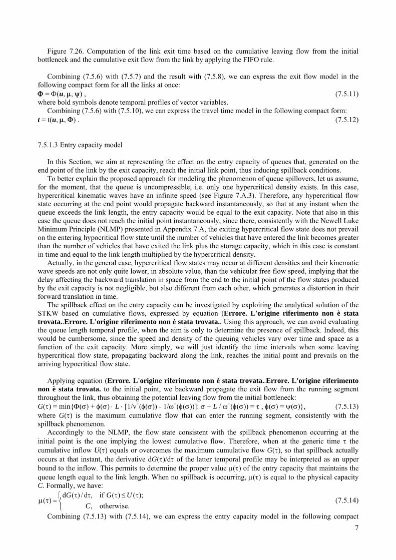
Therefore, the link exit time t(τ) at time τ is obtained, as depicted in Figure 7.26, by applying equation (Errore. L'origine riferimento non è stata trovata..Errore. L'origine riferimento non è stata trovata. to the sequence of the sole running segment and final bottleneck, i.e. without the initial bottleneck, through the following implicit expression: Φ(t(τ)) = Γ(τ) . (7.5.9)

This way we avoid to compute twice the initial bottleneck delay; moreover, at the solution of the DNL (i.e. at equilibrium, in this case) the entry capacity constraint u(τ) ≤ μ(τ) is satisfied at any time τ, and thus such delay is null.

In presence of time intervals with null flow, equation (7.5.9) does not allow to obtain a univocal value of the exit time. To take these circumstances into account, once the cumulative exit flow temporal profile is known, the exit time temporal profile is calculated conventionally as: t(τ) = max{τ + L / v°(0), min{σ: Φ(σ) = Γ(τ)}} , (7.5.10) where L / v°(0) is the free flow travel time of the running segment.

Γ(τ)

τ' t(τ')

Γ(τ') = Λ(σ') = Φ(t(τ'))

time

vehicles

σ'

Λ(τ)

Φ(τ)

7

Figure 7.26. Computation of the link exit time based on the cumulative leaving flow from the initial bottleneck and the cumulative exit flow from the link by applying the FIFO rule.

Combining (7.5.6) with (7.5.7) and the result with (7.5.8), we can express the exit flow model in the

following compact form for all the links at once: Φ = Φ(u, μ, ψ) , (7.5.11) where bold symbols denote temporal profiles of vector variables.

Combining (7.5.6) with (7.5.10), we can express the travel time model in the following compact form: t = t(u, μ, Φ) . (7.5.12)

7.5.1.3 Entry capacity model In this Section, we aim at representing the effect on the entry capacity of queues that, generated on the

end point of the link by the exit capacity, reach the initial link point, thus inducing spillback conditions. To better explain the proposed approach for modeling the phenomenon of queue spillovers, let us assume,

for the moment, that the queue is uncompressible, i.e. only one hypercritical density exists. In this case, hypercritical kinematic waves have an infinite speed (see Figure 7.A.3). Therefore, any hypercritical flow state occurring at the end point would propagate backward instantaneously, so that at any instant when the queue exceeds the link length, the entry capacity would be equal to the exit capacity. Note that also in this case the queue does not reach the initial point instantaneously, since there, consistently with the Newell Luke Minimum Principle (NLMP) presented in Appendix 7.A, the exiting hypercritical flow state does not prevail on the entering hypocritical flow state until the number of vehicles that have entered the link becomes greater than the number of vehicles that have exited the link plus the storage capacity, which in this case is constant in time and equal to the link length multiplied by the hypercritical density.

Actually, in the general case, hypercritical flow states may occur at different densities and their kinematic wave speeds are not only quite lower, in absolute value, than the vehicular free flow speed, implying that the delay affecting the backward translation in space from the end to the initial point of the flow states produced by the exit capacity is not negligible, but also different from each other, which generates a distortion in their forward translation in time.

The spillback effect on the entry capacity can be investigated by exploiting the analytical solution of the STKW based on cumulative flows, expressed by equation (Errore. L'origine riferimento non è stata trovata..Errore. L'origine riferimento non è stata trovata.. Using this approach, we can avoid evaluating the queue length temporal profile, when the aim is only to determine the presence of spillback. Indeed, this would be cumbersome, since the speed and density of the queuing vehicles vary over time and space as a function of the exit capacity. More simply, we will just identify the time intervals when some leaving hypercritical flow state, propagating backward along the link, reaches the initial point and prevails on the arriving hypocritical flow state.

Applying equation (Errore. L'origine riferimento non è stata trovata..Errore. L'origine riferimento

non è stata trovata. to the initial point, we backward propagate the exit flow from the running segment throughout the link, thus obtaining the potential leaving flow from the initial bottleneck: G(τ) = min{Φ(σ) + φ(σ) ⋅ L ⋅ [1/v+(φ(σ)) - 1/ω+(φ(σ))]: σ + L / ω+(φ(σ)) = τ , φ(σ) = ψ(σ)}, (7.5.13) where G(τ) is the maximum cumulative flow that can enter the running segment, consistently with the spillback phenomenon.

Accordingly to the NLMP, the flow state consistent with the spillback phenomenon occurring at the initial point is the one implying the lowest cumulative flow. Therefore, when at the generic time τ the cumulative inflow U(τ) equals or overcomes the maximum cumulative flow G(τ), so that spillback actually occurs at that instant, the derivative dG(τ)/dτ of the latter temporal profile may be interpreted as an upper bound to the inflow. This permits to determine the proper value μ(τ) of the entry capacity that maintains the queue length equal to the link length. When no spillback is occurring, μ(τ) is equal to the physical capacity C. Formally, we have:

d ( ) / d , if ( ) ( );( )

, otherwise.G G U

Cτ τ τ ≤ τ⎧

μ τ = ⎨⎩

(7.5.14)

Combining (7.5.13) with (7.5.14), we can express the entry capacity model in the following compact

8

form11: μ = μ(u, ψ, Φ ; C) . (7.5.15)

7.5.1.4 Fixed-point formulation of the NPM

Figure 7.27. Variables and models of the fixed point formulations for the NPM (left hand side) and for the

DTA with spillback (right hand side) in terms of link flows f = (u, w). The NPM allows determining (see Figure 7.23 and the left hand side of Figure 7.27), for given link flows,

link travel times and capacities consistent with the traffic flow theory that ensure the propagation of congestion through the network. It can be formulated by combining (7.5.11) and (7.5.5) with (7.5.15), yielding a following fixed point problem in terms of entry capacity temporal profiles: μ = μ(u, ψ(u, w, μ ; S), Φ(u, μ, ψ(u, w, μ ; S)) ; C) . (7.5.16)

Although not formally proved, the above fixed-point problem behaves like a contraction and converges in a few iterations to a solution. However, when the travel demand is very high, a solution may not exist due to the possible prevalence of gridlocks, that are queues spilling over intersections that generated them12. For given link flows, the solution to (7.5.16), if any, is denoted as follows: μ = μ*(u, w) . (7.5.17)

Combining (7.5.17) with (7.5.5), the result and (7.5.17) with (7.5.11), the result and (7.5.17) with (7.5.12), yields a performance function, expressing the link exit times in terms of the link flows:

11 The dependency of μ from ψ is solely due to the need of backward propagating only the hypercritical portions of the exit flow temporal profile. 12 This problem can be alleviated by a proper setting (raising) of priority coefficients to favor circulation in roundabouts and other close cycles of the graph.

p(z, c, t) D

ϕ(p, t ; D)

p

ĉ(t)

f t c

z

z(c, t)

network loading map

link performance model

μ*( f)

ψ( f, μ)

t( f, μ, W)

W(f, μ, ψ)

μ

W

ψ

μ

μ( f, ψ, W; C)

ψ

network performance model

C

S f

W

W(f, μ, ψ)

ψ( f, μ; S)

9

t = t(u, μ*(u, w), Φ(u, μ*(u, w), ψ(u, w, μ*(u, w) ; S))) = t*(u, w) . (7.5.18) The cost for users entering a link at any given time is assumed to depend on the travel time at that instant¸

then in compact form we have: c = ĉ(t) . (7.5.19)

Finally, substituting (7.5.18) in (7.5.19), we obtain: c = ĉ(t*(u, w)) = c*(u, w) , (7.5.20) which jointly with (7.5.18) expresses synthetically the LPM.

7.5.2 Network loading map and fixed-point formulation of the equilibrium model In the following, we briefly addresses both route choice and network flow propagation by adopting an

implicit path enumeration approach. Referring to users traveling towards a single destination d, the formulation is based on the concepts of link conditional probability and node satisfaction, whose notation and definitions are introduced below:

pad(τ) probability of using link a, conditional on crossing node TL(a) at time τ;

zxd(τ) expected value of the maximum perceived utility at time τ, relative to the paths Kxd connecting

node x to d which are considered by the user. It can be proved that the following expressions of the node satisfaction and of the link conditional

probability are consistent with a Logit route choice model in which users consider all and only “efficient” paths (a path is efficient if each one of its links is efficient):

( )( ) ( ) ( )( )

( )( )ln exp

da aHD ad

xa FS x EA d

c z tz

∈ ∩

⎛ ⎞⎛ ⎞− τ + τ⎜ ⎟⎜ ⎟τ = θ ⋅

⎜ ⎟⎜ ⎟θ⎝ ⎠⎝ ⎠∑ , if x ≠ d ; 0, otherwise , (7.5.21)

( )( ) ( ) ( )( ) ( ) ( )

expd d

a aHD a TL ada

c z t zp

⎛ ⎞− τ + τ − τ⎜ ⎟τ =⎜ ⎟θ⎝ ⎠

, if a∈EA(d) ; 0, otherwise , (7.5.22)

where EA(d) is the set of the efficient links, that get closer to the destination with reference to a “distance” pattern on the network which is constant in time.

The solution of the triangular system formed by the equations (7.5.21) in topological order, combined with the equations (7.5.22), yields the route choice model, which can be expressed in compact form as: z = z(c, t) , (7.5.23) p = p(z, c, t) . (7.5.24)

Similar expressions can be derived for the deterministic case: zx

d(τ) = max{-ca(τ) + zHD(a)d(ta(τ)): a∈FS(x)∩EA(d)} , if x ≠ d ; 0, otherwise , (7.5.25)

pad(τ) ⋅ [zx

d(τ) + ca(τ) - zHD(a)d(ta(τ))] = 0 , if a∈EA(d) ; 0, otherwise , (7.5.26)

where by definition it is pad(τ) ≥ 0 and :

∑a∈FS(x) pad(τ) = 1 . (7.5.27)

Since the solution to the system (7.5.26)-(7.5.27) is non unique, when more than one link exiting from node x yields the maximum utility zx

d(τ), the symbol “=” in equations (7.5.24) should be replaced by the symbol “∈”. The generalization of the deterministic route choice model to the case where the set of alternatives coincides with all acyclic paths is available but out of the scope of this outline. Moreover, the deterministic model can be exploited within a Monte Carlo simulation to address the case of Probit route choice.

We assume that the origins and the destinations are connected to the rest of the network by dummy links

or infinitesimal length with an infinite physical and saturation capacities, so that for all other nodes the flow conservation equation holds.

Therefore, the inflow uad(τ) on the generic link a is given by the link conditional probability pa

d(τ) multiplied by the flow exiting from node TL(a). The latter is given, in turn, by the sum of the outflow wb

d(τ) from each link b∈BS(TL(a))∩EA(d) of its efficient backward star. While, the inflow uFS(o)

d(τ) on the dummy link FS(o) exiting from origin o is instead equal to the demand flow Do

d(τ) from o to d. Then we have: ua

d(τ) = DHD(a)d(τ), if TL(a) in an origin ; ua

d(τ) = pad(τ) ⋅ ∑ b∈BS(TL(a))∩EA(d) wb

d(τ), otherwise. (7.5.28) Based on equation (Errore. L'origine riferimento non è stata trovata..Errore. L'origine riferimento

10

non è stata trovata., given the exit time temporal profile of link a, the outflow is related to the inflow temporal profile as follows: wa

d(ta(τ)) = uad(τ) / [dta(τ)/dτ] , (7.5.29)

where the weight dta(τ)/dτ stems from the fact that users enter the link at a certain rate and exit it at a different rate, which is higher than the previous one, if the travel time is decreasing, and lower, otherwise.

Obviously, ua(τ) and wa(τ) are given by the sum for all destinations of uad(τ) and wa

d(τ), respectively. The solution of the triangular system formed by the equations (7.5.28)-(7.5.29) in reverse topological

order, yields the network flow propagation model, which can be expressed in compact form as: (u, w) = ϕ(p, t ; D) . (7.5.30)

Combining (7.5.23) with (7.5.24) and the result with (7.5.30) yields a formulation based on implicit path

enumeration of the NLM: (u, w) = ϕ(p(z(c, t), c, t), t ; D) = ϕ*(c, t ; D) . (7.5.31)

On this basis the DTA can be formalized (see Figure 7.27) as a fixed-point problem in terms of link flow temporal profiles by substituting into the NLM (7.5.31) the LPM (7.5.18)-(7.5.20): (u, w) = ϕ*(c*(u, w), t*(u, w); D) . (7.5.32)

The above fixed-point problem can be, as usual, solved by means of an MSA. Reference notes The formulation reported in Section 7.5 is taken from Bellei et al. (2005) and Gentile et al. (2004, 2007),

where solution algorithms are also devised. 1. Bellei G., Gentile G., Papola N. (2005) A within-day dynamic traffic assignment model for urban road

networks. Transportation Research Part B 39, 1-29. 2. Gentile G., Meschini L., Papola N. (2004) Fast heuristics for continuous dynamic shortest paths and all-

or-nothing assignment. Presented at AIRO 2004, Lecce, Italy. 3. Gentile G., Meschini L., Papola N. (2007) Spillback congestion in dynamic traffic assignment: a

macroscopic flow model with time-varying bottlenecks. Transportation Research Part B 41, 1-29.