Centre de Referència en Economia Analítica

Barcelona Economics Working Paper Series

Working Paper nº 154

Can consumption spillovers be a source of equilibrium indeterminacy?

Jaime Alonso-Carrera, Jordi Caballé and Xavier Raurich

July 2007

Can consumption spillovers be a source of equilibriumindeterminacy?

Jaime Alonso-CarreraDepartamento de Economia Aplicada and RGEA

Universidade de Vigo

Jordi CaballéUnitat de Fonaments de l’Anàlisi Economica and CODE

Universitat Autònoma de Barcelona

Xavier RaurichDepartament de Teoria Econòmica and CREB

Universitat de Barcelona

July 20, 2007

Abstract

In this paper, we show that consumption externalities are a source of equilibriumindeterminacy in a growth model with endogenous labor supply. In particular,when the marginal rate of substitution between own consumption and the others’consumption is constant along the equilibrium path, the equilibrium does not ex-hibit indeterminacy. In contrast, when that marginal rate of substitution is notconstant, the equilibrium may exhibit indeterminacy even if the elasticity of thelabor demand is smaller than the elasticity of the Frisch labor supply.

JEL classification codes: D91, E62, O40.

Keywords: consumption externalities, labor supply, indeterminacy.

We are grateful to Thomas Seegmuller, an anonymous referee of this journal, and participantsin the International Conference on Instability and Fluctuations in Intertemporal Equilibrium Mod-els (Marseille) and the XXX Simposio de Analisis Economico (Murcia) for their useful comments.Financial support from the Spanish Ministry of Education and FEDER through grants SEJ2005-03753 and SEJ2006-05441; the Generalitat of Catalonia through the Barcelona Economics program(XREA) and grants SGR2005-00447 and SGR2005-00984; and the Xunta de Galicia through grantPGIDIT06PXIC300011PN are gratefully acknowledged.

Correspondence address: Jordi Caballé. Universitat Autònoma de Barcelona. Departamentd’Economia i d’Història Econòmica. Edifici B. 08193 Bellaterra (Barcelona). Spain.Phone: (34)-935.812.367. Fax: (34)-935.812.012. E-mail: Jordi.Caballe@uab.es

1. Introduction

In this paper we study how the introduction of average consumption in the utilityfunction modifies the determinacy of the equilibrium path of the one sector growthmodel. That average consumption generates an externality resulting on either anincrease or a reduction in the felicity that each individual obtains from his ownconsumption. According to Dupor and Liu (2003), this means that individuals couldexhibit either altruism or jealousy. Moreover, consumption externalities may alsoincrease or reduce the marginal rate of substitution between own consumption andleisure. Thus, we will consider a model encompassing the “keeping-up with the Joneses”and the "running away from the Joneses" features considered by Dupor and Liu (2003).

Several authors have studied the uniqueness of the equilibrium path of the one-sector growth model when the labor supply is endogenous and production externalitiesare introduced. In particular, Benhabib and Farmer (1994) show that the equilibriumof the model with separable instantaneous utility may exhibit indeterminacy whenthe labor supply and the labor demand cross with the wrong slopes. If the laborsupply is upward sloping, the condition for indeterminacy will require a su cientlylarge degree of returns to labor so that the labor demand ends up being upward sloping.However, Bennett and Farmer (2000) argue that the required degree of returns to laboris not plausible. These authors show that if preferences are non-separable betweenconsumption and leisure, then indeterminacy can arise when the labor demand and thelabor supply cross with the normal slopes. In this case, the necessary condition forindeterminacy is that the elasticity of the labor demand is larger than the elasticityof the Frisch labor supply.1 Thus, if the production function exhibits non-increasingreturns to labor, indeterminacy requires that the Frisch labor supply has a negativeelasticity, i.e., it must be downward sloping. However, as shown by Hintermaier (2003),the indeterminacy condition obtained by Bennett and Farmer (2000) implies that theutility function is not concave. In fact, Hintermaier shows that, if the utility functionis concave, the Frisch labor supply will be upward sloping and the equilibrium of theone sector growth model with production externalities will not exhibit indeterminacy.2

In this paper, we will analyze whether the introduction of consumption externalitiescan cause the indeterminacy of the equilibrium path under a concave utility functionand a production function that does not exhibit increasing returns to labor. Liu andTurnovsky (2005) show that consumption externalities do not generate indeterminacyof the equilibrium path when the labor supply is exogenous. Therefore, we will assumeinstead that the labor supply is endogenous and we will show that, in this case,consumption externalities can give rise to equilibrium indeterminacy. In particular,we will show that the indeterminacy of the equilibrium path depends on the restrictedhomotheticity property of the utility function (RH property henceforth). We say thatthe utility function satisfies this property when the marginal rate of substitution (MRS)between consumption and consumption spillovers is constant along the equilibriumpath. In this case, the equilibrium does not exhibit indeterminacy. In contrast, whenthe utility function does not satisfy the RH property, the equilibrium may exhibit

1The Frisch labor supply is defined as the labor supply resulting from keeping the marginal utilityof consumption constant.

2Lloyd-Braga et al. (2006) extend this analysis to technologies with factor-specific external e ects.

1

indeterminacy even though the elasticity of the Frisch labor supply is larger than theelasticity of the labor demand.

Consumption externalities are a source of equilibrium indeterminacy if the equilib-rium interest rate rises when agents coordinate to increase their savings. In this case,starting with an arbitrary equilibrium path, another can be constructed by increasingsavings because the rate of return of capital increases accordingly so as to justify itshigher rate of accumulation. We show that this positive relationship between savingand interest rate may arise when an increase in the amount of saving causes an increasein the next period equilibrium employment, which in turn requires that consumptionexternalities a ect the labor supply. Depending on the e ect of consumption exter-nalities on the labor supply, we can distinguish two regions of indeterminacy. In oneof these regions, the indeterminacy condition of Bennett and Farmer (2000) does nothold and the Frisch labor supply can even be upward slopping. In the other region, theBennett and Farmer condition holds even though the utility function is concave. Thus,consumption externalities make a downward slopping Frisch labor supply compatiblewith a concave utility function. We conclude that indeterminacy can only arise whenconsumption externalities modify the Frisch labor supply, which requires that the util-ity function is non-separable between consumption and leisure. In fact, we prove thatthe kind of separability that prevents indeterminacy from arising is the one implied bythe RH property.

The result that the only presence of consumption externalities may be a sourceof equilibrium indeterminacy in the one-sector growth model is in contrast with thenegative result obtained by Guo (1999), who showed that consumption externalitiesare not a source of equilibrium indeterminacy. However, Guo considers in his analysisan instantaneous utility function that satisfies the RH property and, in this case,consumption externalities do not cause equilibrium indeterminacy. Weder (2000) alsoconsiders a model with consumption externalities and an utility function that satisfiesthe RH property. In his model productive externalities are thus needed to obtainindeterminacy of the dynamic equilibrium.

The rest of the paper is organized as follows. Section 2 describes the economy andcharacterizes the equilibrium path. Section 3 analyzes the uniqueness of the equilibriumpath. Section 4 studies the mechanism that causes equilibrium indeterminacy. Finally,Section 5 concludes the paper. All the proofs appear in the Appendix.

2. The economy

We consider an infinite horizon, continuous time, one-sector model with capitalaccumulation. The economy consists of competitive firms and a representativehousehold.

2.1. Firms

We assume that the unique good of this economy is produced by means of a neoclassicalproduction function with constant returns to scale. For simplicity in the exposition,and without loss of generality, we consider a Cobb-Douglas production function. Hence,per capita output is given by = 1 with (0 1) and where and are the

2

per capita stock of capital and the employment, respectively. The depreciation rate ofcapital is (0 1) As firms behave competitively, profit maximization implies thatthe rental prices of the two inputs equal their marginal productivities,

= 1 1 (2.1)

and= (1 ) (2.2)

2.2. Household

We assume that the representative household is endowed in each period with one unitof time that can be devoted either to supply the amount of labor or to enjoy theamount 1 of leisure. The objective of the household is to maximizeZ

0( 1 ) (2.3)

where is the own consumption, is the average consumption in the economy, and0 is the subjective discount rate. The instantaneous utility function is twice

continuously di erentiable and satisfies the following properties: 1 ( 1 ) 0

11 ( 1 ) 0 3 ( 1 ) 0 33 ( 1 ) 0 lim 1 ( 1 ) = 0

lim01 ( 1 ) = and

11 ( 1 ) 33 ( 1 ) [ 13 ( 1 )]2 (2.4)

for all 0 3 Condition (2.4) implies that the utility function is jointly concavewith respect to consumption and leisure which, together with the other assumptions,guarantees that the solution to the household’s maximization problem is interior. Wealso assume that consumption and leisure are normal goods.

The introduction of average consumption implies that consumption spillovers a ectthe household’s utility. In particular, preferences exhibit jealously when 2 ( 1 ) 0whereas they display admiration (or altruism) when 2 ( 1 ) 0 Following Du-por and Liu (2003) and Liu and Turnovsky (2005), we will assume that

1 ( 1 ) + 2 ( 1 ) 0

According to Dupor and Liu (2003), preferences correspond to the “keeping-up with theJoneses” formulation when the marginal rate of substitution between own consumptionand leisure raises with average consumption and correspond to the “running away fromthe Joneses” formulation when that marginal rate of substitution decreases.

The representative household maximizes (2.3) subject to the budget constraint

+ = + ˙ (2.5)

Let us denote by the Lagrangian multiplier of this maximization problem. Then, thefirst order conditions are

1 ( 1 ) = (2.6)3From now on, the subindex of a function will refer to the position of the argument with respect to

which the partial derivative is taken.

3

3 ( 1 ) = (2.7)

=˙

(2.8)

and the transversality condition is

lim = 0 (2.9)

Combining (2.6) and (2.7), we obtain

3 ( 1 )

1 ( 1 )= (2.10)

Equation (2.6) shows that the Lagrangian multiplier is equal to the discountedmarginal utility of private consumption, (2.8) is the Keynes-Ramsey equation thatshows the intertemporal trade-o between consuming today and consuming in thefuture, and (2.10) drives the intratemporal trade-o between consumption and leisure.Therefore, (2.10) characterizes the labor supply.

2.3. The competitive equilibrium

We are going to obtain the dynamic equations characterizing the equilibrium path. Tothis end, we combine (2.2) and (2.10) to get

3 ( 1 )

1 ( 1 )= (1 ) (2.11)

After evaluating the previous equation at a symmetric equilibrium (i.e., when = )we obtain an equation that implicitly defines the mapping = ( ) from capital andemployment to consumption. Let us di erentiate equation (2.11) with respect to timeand evaluate it at a symmetric equilibrium to obtain

[ ( ) + ( )]

μ˙¶+ [ ( ) ( ) + ]

Ã˙!=

Ã˙!

(2.12)

where

( ) =

μ11 + 12

1

¶( ) ;

( ) =

μ13

1

¶;

( ) =

μ13 + 23

3

¶( ) ;

and

( ) =

μ33

3

¶Note that ( ) is the inverse of the intertemporal elasticity of substitution and weassume that ( ) 0. This requires that 11 + 12 0 Moreover, we assume that

[ ( ) ( )] [ ( ) + ( ) + ( )] 0 (2.13)

4

where

( ) =

μ12

1

23

3

¶( )

Inequality (2.13) holds because both consumption and leisure are assumed to be normalgoods.4 Note also that, if ( ) 0 then preferences exhibit the "keeping up withthe Joneses" feature, whereas they exhibit the "running away from the Joneses" featurewhen ( ) 0

We next combine equations (2.1), (2.6) and (2.8) evaluated at a symmetricequilibrium to get

1 1 = ( )

μ˙¶+ ( )

Ã˙!

(2.14)

Moreover, using (2.12) and (2.14), we get

˙=

³˙´ h

( )+ ( )( )

i £1 1

¤+ ( )

(2.15)

where

( ) = ( )( )

( )

¸( )

is the price elasticity of the Frisch labor supply. Recall that the Frisch labor supply isthe labor supply obtained when the marginal utility of consumption is kept constant.Thus, to obtain that elasticity just note from (2.10) that the labor supply evaluated ata symmetric equilibrium can be written as

( 1) =3 [ ( 1 ) ( 1 ) 1 ]

1(2.16)

where the upper bar in the marginal utility of consumption means that we keep itconstant, and the function ( 1 ) is obtained implicitly from

1 ( 1 ) 1 = 0 (2.17)

Then, the elasticity of the Frisch labor supply is

( ) =1( 1)

( 1)

Finally, from (2.1), (2.2), and (2.5), we obtain the resource constraint

˙ = 1 ( ) (2.18)

where ( ) is implicitly defined in (2.11).Given an initial condition 0 a competitive equilibrium is a path of employment

and capital that solves the system of di erential equations formed by (2.15) and (2.18)

4 Inequality (2.13) follows from applying the implicit function theorem in (2.11) and setting

(1 ) 31

0

5

with (0 1) and that satisfies the transversality condition (2.9). Note that is nowthe control variable, whereas is the state variable.

Let us index the di erent interior steady states by and let be a steady statevalue of employment. Then, according to (2.15), a steady state value of capital will begiven by

= ( )

μ+

¶ 11

(2.19)

Therefore, using (2.18), we immediately see that the steady state values of employmentmust solve the following equation:

( ) [ ( )] 1 ( ) ( ( ) ) = 0 (2.20)

We denote the steady state values of the variables by means of a star and, hence,= ( ) = ( ) = ( ) = ( ) = ( )= ( ) = ( ) and = ( ) are the values of the corresponding

variables at the steady stateThe existence and uniqueness of interior steady states depend on the properties of

the mapping ( ( ) ) In absence of externalities, the assumption on the normality ofconsumption and leisure implies by definition that consumption is a decreasing functionof labor. Hence, since the net output is an increasing function of employment,equation (2.20) has at most a solution in the open interval (0 1). Moreover, observethat the unique steady state satisfies that 0 ( ) 0 This property implies that netinvestment increases with employment around the steady state, which is equivalent tosay that the elasticity of consumption with respect to gross output is smaller than oneat the steady state.5

Condition (2.13) implies that the demand of consumption depends negatively onemployment. However, in the presence of consumption externalities, this conditiondoes not impose any restriction on the equilibrium relationship between consumptionand employment. More precisely, in that case equation (2.11) can implicitly defineconsumption as an increasing function of employment or even as a set-valued mappingof consumption to employment. In these cases, equation (2.20) can have multiplesolutions in the open interval (0 1) and the relationship between net investmentand employment at these interior steady states is ambiguous.

From now on, we will assume that 0 ( ) 0 Although condition (2.13) does notimply that in equilibrium consumption decreases with employment, we assume thatthe increase in consumption is smaller than the increase in net production so thatthe amount of net investment raises with employment. However, this condition doesnot impede the existence of multiple interior steady states when (2.11) defines a set-valued mapping from employment to consumption. To see this, consider the following

5Constant returns to scale imply that output depends linearly on employment at the steady state.By using this property and (2.20), we get that the elasticity of consumption with respect to output atthe steady state is smaller than one if and only if 0( ) 0.

6

instantaneous utility function:6

( 1 ) =

¡ ¢1 ¡1 + 2

¢ (1 )

1(2.21)

which always satisfies (2.13), and is jointly concave with respect to consumption andleisure when (1 + ) and 0 The next result characterizes the existence ofinterior steady states for the economy with this particular utility.

Proposition 2.1. Assume that the utility function has the functional form (2.21), anddefine

1 =(1 )

¸μ+

¶1

2 =(1 ) +

¸μ+

¶ 11

= [(1 + 2 1) 2 2]2 and = 1 2 where 0 Then, there are no interior

steady states either if 2 1 1 and or if 2 1 1 and There are twointerior steady states if 2 1 1 and Otherwise, there is a unique interiorsteady state.

By using (2.10), it is easy to show that the elasticity of the labor supply withrespect to the wage is equal to 1 2 in the economy with the utility function (2.21).Then, according to Proposition 2.1, there is a unique interior steady state when thiselasticity is lower than one, whereas multiple interior steady states may exits when thiselasticity is larger than one and the intensity of consumption externalities, measuredby the parameter is su ciently large.

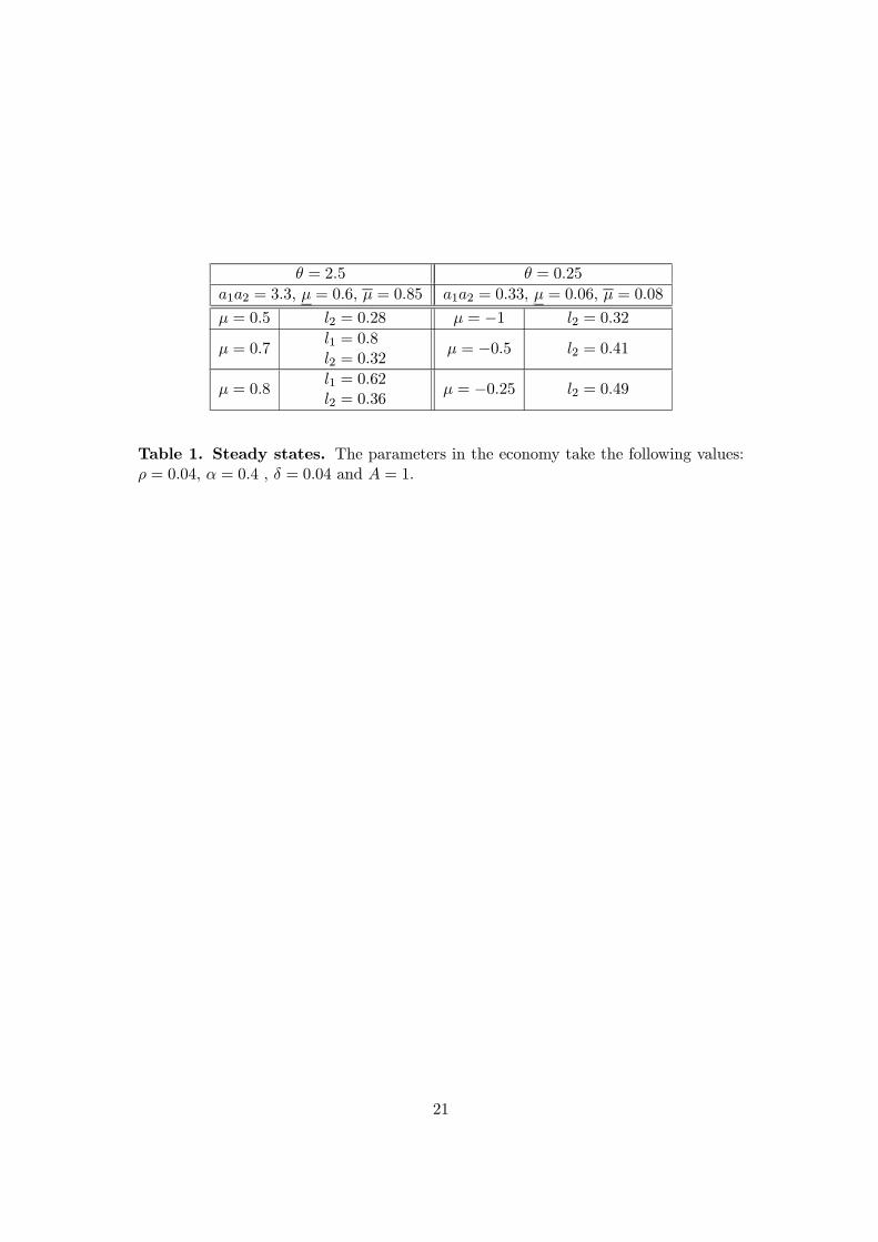
Table 1 provides the steady state values of employment of this economy for severalnumerical examples. We construct these examples as follows. First, we set = 0 4= 0 04 and = 0 04 so that our economy replicates at the steady state a labor income

share of 0 6 a consumption-output ratio of 0 8 and a net interest rate of 0 04. Second,we set the e ciency parameter = 1 Third, the parameters and do not a ect thesteady state value of employment, but their value should be set so that the followingconditions are satisfied: (i) the utility function is concave; (ii) 1 + 2 0; and (iii)

0. The numerical examples in Table 1 satisfy these conditions when = 1 and1 7 Finally, the parameters and are set to replicate the di erent configurations

of interior steady states given in Proposition 2.1. In particular, we consider two di erentvalues of : (i) = 2 5 for which the elasticity of labor supply is larger than one; and(ii) = 0 25 for which the elasticity of labor supply is smaller than one. When = 2 5

6The utility function (2 21) could be generalized to

( 1 ) =

1(1 + ) (1 )

1

We have considered the particular case with = 2 since this allows us both to have a reasonablenumber of subcases in the statement of Proposition 2.1 and to write the statement in tems of the deepparameters of the model. Obviously, the case = 1 is much more simple but generates only one regionof indeterminacy instead of the two indeterminacy regions appearing when = 2 (see Proposition 3.3).

7

two interior steady states exist if 0 6 For the case with = 0 25 there is a uniqueinterior steady state if 0 06 whereas no interior steady states exists when 0 06In these examples, all the interior steady states satisfy the condition 0( ) 0

[Insert Table1]

3. Existence of local indeterminacy

In this section we show that consumption externalities can be a source of equilibriumindeterminacy and we will also provide a su cient condition on the instantaneous utilityfunction that guarantees the uniqueness of the equilibrium path. For that purpose, wefirst linearize the law of motions (2.15) and (2.18) around each interior steady state tofind the local stability properties of these steady states. In this way, we obtain in theAppendix that the trace and the determinant of the Jacobian matrix of the linearizeddynamic system are respectively given by

( ) =

μ+

+

¶( ) (3.1)

and

( ) = (1 ) ( + ) [(1 ) + ]+ +

( + )

¸(3.2)

where

( ) = (1 )

μ ¶(1 ) +

+

¸μ ¶ μ+

¶( + )

By using (3.1) and (3.2), we directly obtain the following result on the stabilityproperties of the steady state equilibria:

Proposition 3.1. Given any steady state(a) the steady state is unstable when one of the following two sets of conditions

holds:(i) + 0 + + 0 and ( ) 0;(ii) + 0 + + 0 and ( ) 0

(b) the steady state is locally saddle-path stable when one of the following two setsof conditions holds:

(i) + 0 and + + 0;(ii) + 0 and + + 0

(c) the steady state is locally stable when one of the following two sets of conditionsholds:

(i) + 0 + + 0 and ( ) 0;(ii) + 0 + + 0 and ( ) 0

The dynamic equilibrium exhibits local indeterminacy when the steady state islocally stable and, thus, Proposition 3.1 shows that consumption spillovers can makethe dynamic equilibrium locally indeterminate. This result is obtained when three

8

reasonable assumptions are imposed: (i) the utility function is concave, (ii) consumptionand leisure are normal goods, and (iii) the production function exhibits constant returnsto scale. Moreover, indeterminacy may arise in two di erent regions of the parameterspace that are separated by the equation = The right hand side of this equationis the elasticity of the labor demand and the left hand side is the elasticity of the Frischlabor supply at the steady state.

In the first region, indeterminacy arises when 0 and, hence, theFrisch labor supply has a negative slope. A crucial contribution of this result is thatindeterminacy in this region is possible with a concave utility function. Note that, since11 + 12 0 the inequality 0 implies that

13 23 12 33 33 11 ( 13)2 0

where the last inequality follows from the concavity condition (2.4). If consumptionexternalities are not present, then 12 = 23 = 0 and the two inequalities cannot besimultaneously satisfied. Thus, consumption spillovers make compatible the existenceof a downward-sloping Frisch labor supply with a concave utility function. This is instark contrast with the indeterminacy configuration derived by Bennett and Farmer(2000). These authors show that the equilibrium exhibits indeterminacy in a modelwithout consumption externalities when production externalities are su ciently largeand However, as Hintermaier (2003) shows, in their model indeterminacyrequires that the utility function be non-concave. Therefore, our result complementsthe uniqueness result obtained by Hintermaier (2003) in a model without consumptionexternalities. This author shows for the case of a Cobb-Douglas production functionthat, if utility function is concave, then the equilibrium does not exhibit indeterminacyeven though production externalities are present.

In the second region, indeterminacy arises when and, hence, the Frischlabor supply may be upward sloping. Note that the related literature says thatindeterminacy from production externalities requires a downward-sloping Frisch laborsupply function. However, we show that consumption spillovers can lead to equilibriumindeterminacy even when this supply function is upward sloping. Observe that in thecase with , indeterminacy arises when + + 0 This conditioncan only be satisfied if consumption spillovers are introduced. To see this, let us assumethat there are no consumption externalities. In this case, the concavity condition (2.4) isgiven by + 0 and condition (2.13) becomes ( + ) ( ) 0 . Thus,if we assume that then + 0 This means that 0 as 0Moreover, since there are no consumption spillovers, we end up having 23 = 0 and

0 which means that 13 0 . This in turn implies that 0 In this case,the concavity condition (2.4) only holds when which contradicts our initialassumption. This means that and condition (2.13) implies that + 0Therefore, the indeterminacy condition + + 0 is not satisfied in absenceof consumption externalities.

The uniqueness of the equilibrium path will depend on the assumptions made onthe utility function. In what follows, we provide a su cient condition on the utilityfunction that implies the uniqueness of the equilibrium path. To this end, we definethe concept of restricted homotheticity (RH). We say that the utility function satisfiesthe RH property if the marginal rate of substitution between consumption and average

9

consumption is constant along the equilibrium path (i.e., when = ). This means that

2( 1 )

1( 1 )= (3.3)

for some constant . The RH property requires the following conditions at a symmetricequilibrium (with = ): (i) the marginal utilities 1 and 2 must be homogenous of thesame degree with respect to consumption; and (ii) the utility must be either additivelyor multiplicatively separable between consumption and leisure. The next result showsthat consumption externalities do not give raise to equilibrium indeterminacy when theutility function satisfies the RH property:

Proposition 3.2. The equilibrium does not exhibit indeterminacy when the utilityfunction satisfies the RH property

As can be seen in the proof of Proposition 3.2, the RH property makes the dynamicequations characterizing the competitive equilibrium equivalent to those of the standardRamsey model with no consumption externalities. Thus, the lack of equilibriumindeterminacy of the latter model is inherited by its counterpart with consumptionexternalities satisfying the RH property.

We next illustrate the results in Propositions 3.1 and 3.2 by using the functionalform (2.21) of the utility function. We will look at two cases: (i) = 0 and (ii) 6= 0In the first case, the utility function satisfies the RH property, whereas this propertydoes not hold in the second case. From Proposition 2.1 we know that in the case with= 0 there exists a unique interior steady state with a level of employment given by

=(1 ) ( + )

(1 ) ( + ) + [ (1 ) + ]

Moreover, Proposition 3.2 ensures that this steady state is never locally indeterminate.We now analyze the economy defined by the utility function (2.21) with 6= 0 As

was proved in Proposition 2.1, in this case two interior steady states may emerge, whichwould be given by

1 =h(1 + 1 2 + ) 2 ( 2)

2i

and

2 =h(1 + 1 2 ) 2 ( 2)

2i

where

=h(1 + 1 2)

2 4 ( 2)2i1 2

The next proposition gives the necessary and su cient conditions under which thedynamic equilibrium is locally indeterminate around these steady states.

Proposition 3.3. Assume the instantaneous utility function (2.21) with 6= 0 anddefine

=1

11 2+ (1 ) +

h1 2

11

i1+ 1 2 1

1 2

10

and

=1

μ1 + 2 1

1 + 1 2

¶for = 1, 2 and with 1 =

h³1 + 1 2 +

2

´2 1 2

iand 2 =

h³1 + 1 2

2

´2 1 2

iHence,

(a) The steady state given by 1 is locally stable either if 1 and³

1 1

´or if 1 and

³1 1

´(b) The steady state given by 2 is locally stable either if 1 and

³2 2

´or if 1 and

³2 2

´As shown in Proposition 2.1, when the utility function (2.21) does not satisfy the RH

property, two steady states may exist when the elasticity of the labor supply is largerthan one. Proposition 3.3 shows how the stability properties of each steady state dependon the intensity of the consumption externality, measured by the parameter Notethat the steady states can be locally stable and, in this case, the dynamic equilibriumexhibits local indeterminacy. However, the indeterminacy region is di erent in eachsteady state. From the proof of this proposition, it can be seen that steady state givenby 1 exhibits indeterminacy only when + 1 0 whereas steady state given by 2

exhibits indeterminacy only when + 2 0Table 2 shows the value of the characteristic roots in each steady state when di erent

values of the parameters and are considered. The other parameters are setas in the economy of Table 1. The steady state equilibrium is saddle-path stablewhen the two roots have a di erent sign, and it is unstable when the real part of thetwo roots is positive. When the real part of the two roots takes a negative value,the dynamic equilibrium exhibits indeterminacy. Table 2 shows several examples ofequilibrium indeterminacy. In particular, when = 2 5 = 0 75 = 0 7 and= 0 9 steady state 2 is locally stable. In this case, 2 = 0 32 and the intertemporal

elasticity of substitution is equal to 16 4. Steady state 1 is also locally stable when= 2 5 = 4 = 0 85 and = 4 4 In this case, 1 = 0 51 and the intertemporal

elasticity of substitution is equal to 0 67. These examples show that the equilibriumcan exhibit local indeterminacy when the value of the parameters is plausible and thevalue of the intertemporal elasticity of substitution is low.

[Insert Table 2]

4. Labor supply and indeterminacy

In this section, we explain the economic mechanism underlying the indeterminacy resultdescribed in the previous section. We start by considering the intertemporal trade-obetween consuming today and consuming in the future. In particular, we assume thatthe economy is in an equilibrium path and agents coordinate into a reduction of currentconsumption that reduces current utility and increases future utility through a largeramount of saving. Obviously, the increase in savings can only be an equilibrium decision

11

if the interest rate increases. We proceed to show that consumption externalities cancause a complementarity between the current amount of saving and the next periodamount of employment, which may lead to the necessary increase in the interest ratethat justifies the larger amount of savings. When this occurs, then the equilibrium mayexhibit local indeterminacy.

Note that equation (2.14) implies that consumption externalities modify the path ofsavings either by changing the intertemporal elasticity of substitution or by modifyingthe labor supply. As Liu and Turnovsky (2005) have already shown that the equilibriumpath is unique when the labor supply is exogenous, we will focus the analysis on thee ects of consumption externalities on the Frisch labor supply. We distinguish twodi erent e ects on this labor supply. First, consumption externalities modify the slopeof the Frisch labor supply. Second, they also distort the e ect that changes in privateconsumption have on this labor supply.

In order to understand the e ect of an increase in consumption on the labor supply,we use (2.16) to obtain the elasticity of the Frisch labor supply with respect to themarginal utility of private consumption, that is,

μ1

¶μ1¶=

( 31 + 32)³

1

´3

1

( 31 + 32)¡ ¢

33

μ1¶

where

1=

1

11 + 12

and

=13

11 + 12

as follows from (2.17). Then, using the definitions of and we obtain that in asteady state this elasticity is μ

1

¶μ1¶=

+(4.1)

Moreover, after applying the implicit function theorem to (2.11), we obtain from (2.20)that

0 ( ) =

μ ¶μ+ +

+

¶As we have assumed that 0 ( ) 0 the signs of + and of + +coincide. This implies that the sing of + is di erent in the the two regions forwhich Proposition 3.1 states the existence of local indeterminacy. We proceed to explainthe mechanism driving the complementarity between saving and employment and, thus,the positive e ect of saving on the interest rate, in each region of indeterminacy.

In the first region of indeterminacy, we have + + 0 andThis means that + 0 and 0 and, hence, the elasticity of the labor supplywith respect to the marginal utility of consumption, which is given by (4.1), is negative.As the increase in savings raises future consumption and then reduces next periodmarginal utility, the Frisch labor supply increases in the next period. The increase

12

in the labor supply raises the equilibrium amount of employment since Thisincreases the next period interest rate because the marginal product of capital increaseswith employment. We have then explained the complementarity between savings andemployment, and the corresponding positive relationship between saving and interestrate, in the first region. When this complementarity is su ciently strong, it resultsin equilibrium indeterminacy. Note that, in this region, indeterminacy arises becausethe equilibrium amount of leisure decreases as consumption increases. If consumptionexternalities were not introduced, condition (2.13) would imply that leisure raises withconsumption and the equilibrium would be unique.

In the second region of indeterminacy, we have + + 0 andwhich implies that + 0 However, can be either positive or negative and,therefore, we can distinguish two cases in this region. Assume first that the price elas-ticity of Frisch labor supply is positive, i.e., 0 . In this case, the elasticity of thelabor supply with respect to the marginal utility of consumption given by (4.1) is neg-ative. Then, the labor supply increases as the amount of saving increases, due to thereduction in the next period marginal utility of consumption. As 0 the increasein the labor supply raises the amount of employment in the next period. This makes theinterest rate increase in the next period and we end up obtaining a positive relationshipbetween saving and interest rate. Thus, in this case, indeterminacy is also explainedby the reduction in the equilibrium amount of leisure when consumption raises.

In contrast, when ( 0) the elasticity of labor supply with respect tomarginal utility of consumption given by (4.1) is positive. In this case the increasein saving then reduces the marginal utility of consumption, so that the next periodlabor supply declines. However, since the Frisch labor supply has a negative slope, butits price elasticity is larger than the elasticity of labor demand, the decrease in laborsupply is followed by a decrease in the equilibrium rate of wages that finally drivesemployment up. This causes the increase in the interest rate resulting in indeterminacy.

Consumption externalities may then cause equilibrium indeterminacy becausethey distort the labor market by altering the marginal rate of substitution betweenconsumption and leisure at the equilibrium. In fact, if there were no consumptionexternalities, condition (2.13) would imply that leisure increases with consumption.This means that, as a result of the increase in savings, next period labor supplywould decrease. The reduction in the labor supply would imply a reduction in theamount of employment, because the Frisch labor supply is upward slopping when theutility function is concave and there are no consumption externalities. Obviously, thereduction in employment implies that next period interest rate would decline as agentsincrease savings. This shows that there is a unique equilibrium path in this economywhen there are no consumption externalities.

Condition (2.13) implies that leisure and consumption are normal goods. How-ever, indeterminacy arises when employment increases with consumption along anequilibrium path. It follows that the equilibrium can only exhibit indeterminacy ifconsumption externalities modify the labor supply. This requires that preferences arenon-separable between consumption and leisure. In fact, as shown in Proposition 3.2,the kind of separability that prevents indeterminacy from arising is the one impliedby the RH property. To see this, suppose that consumption externalities have beeninternalized, which implies that the utility function satisfies b ( 1 ) ( 1 ).

13

Then, the labor supply is characterized by

=b3b1 = 3

1 + 2

When the utility function satisfies the RH property, this equation can be rewritten as

(1 + ) =3

1

Note that the Frisch labor supply obtained from this equation has both the same slopeand the same elasticity with respect to the marginal utility of consumption than thelabor supply obtained from equation (2.11). This shows that consumption externalitiesdo not modify the labor supply when the RH property is satisfied, which explains theuniqueness of the equilibrium path in this case.

5. Concluding remarks

In this paper we have analyzed the uniqueness of the dynamic equilibrium of a one-sector growth model when we assume that average consumption a ects individualsfelicity, that is, when consumption externalities are present. We assume thatthe utility function of this model is concave, consumption and leisure are normalgoods, and the production function does not exhibit increasing returns. With theseplausible assumptions, we show that multiple steady states may exist in this economywith consumption externalities. We also show that the equilibrium may exhibitindeterminacy when consumption externalities are introduced. In particular, we showthat the equilibrium path is unique if the utility function satisfies the RH property. Incontrast, if the RH condition does not hold, the equilibrium can exhibit indeterminacy.

We have shown that there are two di erent regions of indeterminacy. In the firstone, the elasticity of the labor demand is smaller than the elasticity of the Frisch laborsupply; whereas the opposite relation holds in the second region. Therefore, whenconsumption externalities are introduced, the equilibrium can exhibit indeterminacyeven if the elasticity of the labor demand is smaller than the elasticity of the Frischlabor supply.

Alonso-Carrera et. al. (2006) show that the equilibrium is ine cient when habitadjusted consumption and consumption externalities are not perfect substitutes, whichsuggests that the interaction between habits and externalities is another potentialsource of equilibrium indeterminacy. Moreover, Chen (2006) shows that the economymay exhibit multiple steady states when a process of habit formation is introduced.Therefore, to study how the interaction between habit formation and consumptionexternalities a ects the uniqueness of the dynamic equilibrium seems a promising lineof future research.

14

References

[1] Alonso-Carrera, J., J. Caballé, and X. Raurich (2006). “Welfare implicationsof the interaction between habits and consumption externalities,” InternationalEconomic Review 47: 557-571.

[2] Alonso-Carrera, J., J. Caballé, and X. Raurich (2007). “Can ConsumptionSpillovers Be a Source of Equilibrium Indeterminacy?” CREA-Barcelona Eco-nomics Working Papers 154.

[3] Benhabib, J. and R. Farmer (1994). “Indeterminacy and Increasing Returns”Journal of Economic Theory, 63: 19-41.

[4] Bennett, R. and R. Farmer (2000) “Indeterminacy with Non-Separable Utility”,Journal of Economic Theory 93: 118-143.

[5] Chen, B-L. (2006). “Multiple BGPs in a Growth Model with Habit Persistence,”Journal of Money, Credit and Banking, forthcoming.

[6] Dupor, B., and W.F. Liu, (2003). “Jealousy and Equilibrium Overconsumption,”American Economic Review 93: 423-428.

[7] Guo, J. T. (1999). “Indeterminacy and Keeping up with the Joneses,” Journal ofQuantitative Economics, 15: 17-27.

[8] Hintermaier, T. (2003). “On the Minimum Degree of Returns to Scale in SunspotModels of the Business Cycle,” Journal of Economic Theory 110: 400-409.

[9] Liu, W.F. and S. Turnovsky (2005). “Consumption Externalities, Production Ex-ternalities and Long-Run Macroeconomic E ciency,” Journal of Public Economics89:1097-1129.

[10] Loyd-Braga, T., C. Nourry and A. Venditti (2006). “Indeterminacy with smallexternalities: the role of non-separable preferences,” forthcoming in InternationalJournal of Economic Theory

[11] Turnovsky, S. (1995). Methods of Macroeconomic Dynamics. MIT Press. Cam-bridge, MA.

[12] Weder, M. (2000). “Consumption Externalities, Production Externalities andIndeterminacy,” Metroeconomica 51: 435-453.

15

AppendixThe linearized dynamic system. Throughout this analysis the variables of themodel are evaluated at a steady state. The Jacobian matrix associated with the systemof di erential equations (2.15) and (2.18) around the steady state is

=

˙ ˙

˙ ˙=

"( )

˙( + )

+

# "( )

˙( + )+

#

where

=( )

=

μ+

¶³ ´=

( )=

μ+

¶³ ´and , and represent the partial derivatives of the production function,with the subindex denoting the argument with respect to which the partial derivativeis taken. The determinant of the Jacobian matrix is

( ) =

μ+

¶μ+

¶( )

μ ¶( )

¸Constant returns to scale imply that = Then, using the expressions forand we obtain

( ) =

μ+

¶μ+

¶ μ ¶( ) +

μ+

¶³ ´¸As constant returns to scale also imply that = + the Cobb-Douglas functionalform for the production function and (2.20) make the previous equation to simplify to(3.2). The trace of the Jacobian matrix is

( ) =

μ1

+

¶ μ+

¶ μ ¶( ) ( ) ( + )

¸By using the expressions for and and the Cobb-Douglas production function and(2.20),we obtain (3.1).

Proof of Proposition 2.1. Consider the utility function (2.21). Then, using (2.19),we obtain

( ) =

μ+

¶ 11

(A.1)

and using (2.11) and (A.1), we obtain

( ) = 21 + 1 (A2)

16

where

1 =

(1 )³+´

1

Finally, using (2.20), it can be shown that the steady-states are the roots of the followingfunction:

( ) 2

μ2 1 + 1

2

¶+ 1

where

2 =(1 ) +

¸μ+

¶ 11

The two roots of ( ) are:

1 =1 + 2 1 +

2 2(A3)

2 =1 + 2 1

2 2(A4)

with =h(1 + 2 1)

2 4 ( 2)2i1 2

Note that if 0 then 1 2 0 whereas if

0 then 1 0 and 2 0 Note also that we can define = ( ). Obviously, ansteady state requires that (0 1) andμ

1 + 2 1

2

¶24

On the one hand, the second condition implies that where

=

μ1 + 2 1

2 2

¶2On the other hand, in order to set conditions that guarantee that (0 1) we

must di erentiate between the two candidates to steady state. First, 1 1 impliesthat

21 1 1 + 1 1

and, using (A3), we obtainq(1 + 2 1)

2 4 22 1 2 1

Note that if 1 2 1 then 1 1 and if 1 2 1 then 1 1 when where= 1

2Second, 1 0 implies that 2

1 1 1 1 and, using (A3), we can rewritethis inequality as

1+ 2 1+ (1+ 2 1)2 4 2

2 0

Obviously, if ( ) 0 then 1 ( ) 0 Next, 2 1 when 22 1 2 + 1 1 Using

(A4), this inequality can be rewritten asq(1 + 2 1)

2 4 22 1 2 1

17

Note that 2 1 when either 1 2 1 or when 1 2 1 and Finally, 2 0when 2

2 1 2 1 which is always satisfied as it can be shown using (A4).

Proof of Proposition 3.2. Let us find the command optimum allocation of our modelwhen consumption externalities are internalized by a social planner. For this problem,the resource constraint is (2.18), which is the same that for the competitive economy.The instantaneous utility faced by the planner will be

b( 1 ) = ( 1 ) (A.1)

The utility b is increasing in under our assumptions on since b1 = 1 + 2 0Moreover, the planner’s marginal utility is decreasing in . To see this, use the RHproperty to compute b11 = (1 + )( 11 + 12) 0

and observe that 0 implies that 11+ 12 0, while 1+ 2 0 together with theRH property (i.e., 1 + 2 = (1 + ) 1) implies that 1 + 0

The first order conditions for the planner’s problem are

1 ( 1 ) (1 + ) = (A.2)

3 ( 1 ) = (1 ) (A.3)

and1 1 =

˙

Dividing (A.3) by (A.2) we obtain

3 ( 1 )

1 ( 1 )= (1 + )(1 )

If we di erentiate the previous equation with respect to time in order to express it interms of the growth rates of and , the term (1 + ) disappears and the resultingequation turns out to be (2.15). Therefore, the dynamic equations characterizing theplanner’s solution are (2.15) and (2.18), which characterize also the solution of theoriginal model where the consumption spillovers are not internalized. Finally, noticethat the planner’s solution coincides with the solution of the standard Ramsey modelwithout consumption externalities when the instantaneous utility function faced byindividuals is (A.1). Since it is well known that the Ramsey model with endogenouslabor supply does not exhibit indeterminacy (see, for instance, Turnovsky, 1995,Chapter 9), the model with consumption externalities satisfying the RH property doesnot display indeterminacy either.

Proof of Proposition 3.3. Assume that 6= 0 Then, by using (2.21) we obtain thatthe following equalities hold at each interior steady state :

= (1 ) (1 )

= (1 )

μ1 + 2

¶18

= (1 + ) (1 ) + [ (1 ) 1] = 1

= [ (1 ) 1]

μ1 + 2

¶and

=2 2

1 + 2

where and are the steady state value of employment and consumption, respectively.From some mechanical algebra we obtain that the interior steady state of this economysatisfies 1 + 2 = 1 and = 1 We then get

=2

1

= (1 )

μ1

1 2

¶= [ (1 ) 1]

μ1

1 2

¶We proceed to obtain parameter conditions that define the di erent stability regions

in Proposition 3.1. First, note that

+ + = 12

1+

1

1 2

Replacing the starionary value of in the previous equation, it follows that + +is negative in steady state given by 1 and positive in steady state given by 2.

Next, + can be rewritten as follows

+ =

μ1

1 2

¶1 + 1 2 (1 )

μ1

¶¸and, using the definition of we obtain that

+ =

μ1

1 2

¶½[ (1 )] (1 + 1 2) (1 ) (1 + 1 2 )

¾Hence, + 0 when either (i) and 1 or (ii) and 1 Finally,( ) can be rewritten as follows

( ) =

μ1

¶+

¸(1 ) + +

¸(1 ) +

+

¸Using the definition of 1 and 2 in Proposition 2.1, we get

(1 ) +

+

¸=(1 ) 1 2

Using this equation and the definitions of and of , ( ) simplifies to

19

( ) = (1 )

μ1

¶+ (1 )

(1 )

1 2

¸(1 )

μ(1 )

+ 1 2 +1

1 2

¶Using the definition of it can be shown that ( ) 0 when either (i)and 1 or (ii) and 1 Otherwise, ( ) 0. Using these conditionsand Proposition 3.1, the statement of Proposition 3.4 follows.

20

= 2 5 = 0 25

1 2 = 3 3 = 0 6 = 0 85 1 2 = 0 33 = 0 06 = 0 08

= 0 5 2 = 0 28 = 1 2 = 0 32

= 0 7 1 = 0 8

2 = 0 32= 0 5 2 = 0 41

= 0 8 1 = 0 62

2 = 0 36= 0 25 2 = 0 49

Table 1. Steady states. The parameters in the economy take the following values:= 0 04 = 0 4 , = 0 04 and = 1

21

= 2 5 = 0 75 = 0 7Steady State 2 Steady State 1

= 0 1 = 0 223

2 = 0 121 = 0 091

2 = 0 36

= 0 9 1 = 0 12 + 0 8

2 = 0 12 0 81 = 0 0906

2 = 0 16

= 1 1 1 = 2 02 0 3

2 = 2 02 + 0 31 = 0 0904

2 = 0 142

= 2 5 = 4 = 0 85Steady State 2 Steady State 1

= 0 1 = 0 07

2 = 0 011 = 0 001

2 = 0 07

= 4 4 1 = 0 25

2 = 0 00561 = 0 845

2 = 0 0134

= 4 5 1 = 0 21

2 = 0 0511 = 0 733

2 = 1 042

= 0 25 = 0 03

Steady State 2= 0 75 = 4

= 0 1 = 0 12

2 = 0 079= 0 1 = 0 0635

2 = 0 023

= 2 1 = 0 0224

2 = 0 169= 0 5 1 = 0 07

2 = 0 053

= 2 76 1 = 0 44 2 4

2 = 0 44 + 2 4= 1 1 = 0 0678

2 = 0 032

Table 2. Stability when 6= 0

22