Optimal Hyper-Scalable Load Balancing with a

Strict Queue Limit

Mark van der BoorEindhoven University of Technology

Sem BorstEindhoven University of Technology

Johan van LeeuwaardenTilburg University, Eindhoven University of Technology

December 16, 2020

Abstract

Load balancing plays a critical role in efficiently dispatching jobs inparallel-server systems such as cloud networks and data centers. A funda-mental challenge in the design of load balancing algorithms is to achievean optimal trade-off between delay performance and implementation over-head (e.g. communication or memory usage). This trade-off has primarilybeen studied so far from the angle of the amount of overhead required toachieve asymptotically optimal performance, particularly vanishing delayin large-scale systems. In contrast, in the present paper, we focus on anarbitrarily sparse communication budget, possibly well below the min-imum requirement for vanishing delay, referred to as the hyper-scalableoperating region. Furthermore, jobs may only be admitted when a specificlimit on the queue position of the job can be guaranteed.

The centerpiece of our analysis is a universal upper bound for theachievable throughput of any dispatcher-driven algorithm for a given com-munication budget and queue limit. We also propose a specific hyper-scalable scheme which can operate at any given message rate and enforceany given queue limit, while allowing the server states to be captured viaa closed product-form network, in which servers act as customers travers-ing various nodes. The product-form distribution is leveraged to provethat the bound is tight and that the proposed hyper-scalable scheme isthroughput-optimal in a many-server regime given the communication andqueue limit constraints. Extensive simulation experiments are conductedto illustrate the results.

1

arX

iv:2

012.

0835

7v1

[cs

.PF]

14

Dec

202

0

1 Introduction

Load balancing provides a crucial mechanism for efficiently distributing jobsamong servers in parallel-processing systems. Traditionally, the primary ob-jective in load balancing has been to optimize performance in terms of queuelengths or delays. Due to the immense size of cloud networks and data centers[13, 20, 28], however, implementation overhead (e.g. communication or mem-ory usage involved in obtaining or storing state information) has emerged asa further key concern in the design of load balancing algorithms. Indeed, thefundamental challenge in load balancing is to achieve scalability: providing fa-vorable delay performance, while only requiring low implementation overheadin large-scale deployments.

The seminal paper [12] approached the above challenge by imposing the nat-ural performance criterion that the probability of non-zero delay vanishes as thenumber of servers grows large. It was shown that this can only be achieved withconstant communication overhead per job when sufficient memory is availableat the dispatcher. There are in fact schemes which achieve a vanishing delayprobability with only one message per job [3, 18, 29] or even fewer [7], but theserely on server-initiated updates as opposed to dispatcher-driven probes. Wedefer a more extensive discussion of these papers and the broader literature toa later stage in this introduction.

In the present paper we pursue the same intrinsic trade-off between perfor-mance and communication overhead, but focus on the optimal performance for apotentially scarce communication budget, and our perspective is fundamentallydifferent in two respects. First of all, we set the admissible message rate δ to bearbitrary, and in particular to be far lower than one message per job, which werefer as the ‘hyper-scalable’ operating regime. This range is especially relevantin scenarios with relatively tiny jobs and a correspondingly massive arrival ratewhich may significantly exceed the message rate that can be sustained betweenthe dispatcher and the servers, prohibiting even just one message per job. Sec-ond, jobs may only be admitted when a strict limit K on the queue positionof the job can be guaranteed. This queue limit K can have any value and isoffered in systems of any size, as opposed to a zero queue length that is only en-sured with high probability in a many-server regime. The combination of a lowcommunication budget per job and a strict admission condition is particularlypertinent for high-volume packet processing applications, where zero delay maynot be feasible given the admissible message rate, but where an explicit queuelimit is crucial.

As the cornerstone of our analysis, we establish a universal upper bound forthe achievable throughput of any dispatcher-driven algorithm as function of δand K, thus capturing the trade-off between performance and communicationoverhead. We also introduce and analyze a specific hyper-scalable scheme whichapproaches the latter bound in a many-server regime, demonstrating that thebound is sharp.

2

Model set-up and hyper-scalable scheme We adopt the set-up of the cele-brated supermarket model which has emerged as the canonical framework in therelated literature (as further reviewed below), but add several salient featuresrelevant for our purposes. Specifically, we consider a system with N identicalservers of unit exponential rate and a single dispatcher where jobs arrive as aPoisson process of rate Nλ. The dispatcher is unaware of the service require-ments of jobs and cannot buffer them, but must immediately forward them toone of the servers or block them. The throughput of the system is defined asthe rate of admitted jobs per server.

The blocking option is relevant since the dispatcher must enforce an explicitqueue limit K, and is only allowed to admit a job and assign it to a server ifit can guarantee that the queue position encountered by that job is at most K.Note that it is not enough for a job to end up in such a position thanks to alucky guess, but that the dispatcher must have absolute certainty in advancethat this is the case, and that a job must be discarded otherwise. Discardingmay be the preferred option in packet processing applications when handlinga packet beyond a certain tolerance window serves no useful purpose. In thatcase, processing an obsolete packet results in an unnecessary resource wastageand needlessly contributes to further congestion, and is thus worse than simplydropping the packet upfront.

As mentioned above, the dispatcher is oblivious of the service requirements,which are exponentially distributed and thus have unbounded support. Hence,the dispatcher critically relies on information provided by the servers in orderto enforce the queue limit K, and is allowed to send probes for this purpose,requesting queue length reports at a rate Nδ. In addition, the dispatcher isendowed with unlimited memory capacity, which it may use to determine whichserver to probe and when or to which server it will dispatch an arriving job.Servers return instantaneous queue length reports in response to probes fromthe dispatcher, but are not able to initiate messages or send unsolicited updateswhen reaching a certain status.

With the above framework in place, we will construct a specific hyper-scalable scheme which is guaranteed to enforce the queue limit K and oper-ate within the communication budget δ. The scheme toggles each individualserver between two modes of operation, labeled open and closed. An open pe-riod starts when the dispatcher requests a queue length update from the serverand the reported queue length is below K; during that period the server is notworking, and waits for incoming jobs from the dispatcher, seeing its queue onlygrow. Once the queue length reaches the limit K, a closed period starts, endingwhen the dispatcher requests the next update after τ time units; during thatperiod the server is continuously working as long as jobs are available, withoutreceiving any further jobs, thus draining its queue. When the queue lengthreported at an update is exactly K, the open period has length zero, and thenext closed period starts immediately. By construction, the above-describedmechanism maintains a queue limit of K at all times and induces a messagerate of at most 1/τ per server, which makes τ = 1/δ the obvious choice.

3

Main contributions The main contributions of the paper may be summa-rized as follows. First of all, we establish a universal upper bound λ∗(δ,K)for the achievable throughput of any dispatcher-driven algorithm subject to thecommunication budget per server in terms of δ and the queue limit K. Theupper bound relies on a simple yet powerful argument which counts the num-ber of jobs that can be admitted per message given the queue limit K and themessage rate δ. While the macroscopic view of the argument covers a broadrange of strategies with possibly dynamic and highly complex update rules, thenature of the upper bound strongly points to the superior properties of constantupdate intervals.

Armed with that insight, we propose a hyper-scalable scheme which canoperate at any given message rate δ and enforce any given queue limit K. Atthe same time, the scheme is specifically designed to produce system dynamicsthat can be represented in terms of a closed product-form queueing network,in which the servers act as customers traversing various nodes. This furnishestractable expressions for the relevant stationary distributions and in particularthe blocking probability. The expression for the blocking probability is usedto prove that the achieved throughput approaches the minimum of the above-mentioned upper bound and the normalized job arrival rate λ in a many-serverregime. This in turn demonstrates that the upper bound is tight and that theproposed hyper-scalable scheme provides optimality in the three-way trade-offamong queue limit, communication and throughput.

Background on load balancing algorithms Load balancing algorithmscan be broadly categorized as static (open-loop), dynamic (closed-loop), or someintermediate blend, depending on the amount of state information (e.g. queuelengths or load measurements) that is used in dispatching jobs among servers.Within the category of dynamic policies, one can further distinguish betweendispatcher-driven (push-based) and server-oriented (pull-based) approaches. Inthe former case, the dispatcher ‘pushes’ jobs to the servers and takes the ini-tiative to collect state information for that purpose, while the servers play apassive role and only provide state information when explicitly requested. Incontrast, in server-oriented approaches, the servers may pro-actively share stateinformation with the dispatcher, and indirectly ‘pull’ in jobs by advertisingtheir availability or load status. The use of state information naturally allowsdynamic policies to achieve better performance, but also involves higher im-plementation complexity (e.g. communication overhead and memory usage) asmentioned earlier. The latter issue has emerged as a pivotal concern due tothe deployment of large-scale cloud networks and data centers with immensenumbers of servers handling massive amounts of service requests.

The celebrated Join-the-Shortest-Queue (JSQ) policy provides the gold stan-dard in the category of dispatcher-driven algorithms and offers strong stochas-tic optimality properties. Specifically, in case of identical servers, exponentiallydistributed service requirements and a service discipline at each server that isoblivious to the actual service requirements, the JSQ policy achieves minimum

4

mean delay among all non-anticipating policies [10, 31]. In order to implementthe JSQ policy, however, a dispatcher relies on instantaneous knowledge of thequeue lengths at all the servers, which may involve a prohibitive communicationburden, and may not be scalable. Related is the join-below-threshold scheme[34], which is throughput-optimal, but the dispatcher-driven variant is not scal-able either.

The latter issue has spurred a strong interest in so-called JSQ(d) strate-gies, where the dispatcher assigns incoming jobs to a server with the shortestqueue among d servers selected uniformly at random. This involves d messageexchanges per job (assuming d ≥ 2), and thus drastically reduces the communi-cation overhead compared to the full JSQ policy when the number of servers Nis large. At the same time, even a value as small as d = 2 yields significantperformance improvements in the many-server regime N → ∞ compared topurely random assignment (d = 1) [22, 30]. This is commonly referred to as the“power-of-two” effect. Similar power-of-d effects have been demonstrated forheterogeneous servers, non-exponential service requirements and loss systems in[8, 9, 25, 26, 27, 32].

Unfortunately, JSQ(d) strategies lack the ability of the conventional JSQpolicy to achieve zero queueing delay as N → ∞ for any finite value of d.In contrast, if d grew with N , making it possible to drive queueing delay tozero [24, 17], the communication overhead would grow unboundedly. A note-worthy exception arises for batches of jobs when the value of d and the batchsize grow suitably large, as can be deduced from results in [33]. Leaving batcharrivals aside though, it is in fact necessary for d to grow with N in order toachieve zero queueing delay, since results in the seminal paper [12] show thatthis is fundamentally impossible with a finite communication overhead per job,unless memory is available at the dispatcher to store state information.

The latter feature is exactly at the core of the so-called Join-the-Idle-Queue(JIQ) scheme [3, 18], where servers advertise their availability by transferring a‘token’ to the dispatcher whenever they become idle, thus generating at mostone message per job. The dispatcher assigns incoming jobs to an idle serveras long as tokens are outstanding, or to a uniformly at random selected serverotherwise. Remarkably, the JIQ scheme has the ability of the full JSQ policyto drive the queueing delay to zero as N → ∞, even for generally distributedservice requirements [11, 29].

Note that for no single value of d, a JSQ(d) strategy can rival the JIQ schemewhich simultaneously provides low communication overhead and asymptoticallyoptimal performance. As alluded to above, this superiority reflects the power ofserver-oriented approaches in conjunction with memory at the dispatcher. Thevalue of memory in load balancing was already studied in [1, 23] in a ‘balls-and-bins’ context. Related work in [21] examines how much load balancingperformance degrades when delayed information is used. A framework for mean-field analysis for JSQ(d) strategies with memory is developed in [19]. Theauthors of [2] use mean-field limits to determine the minimum required valueof d for JSQ(d) strategies with memory to achieve zero queueing delay. Thepossibilities with limited memories are explored in [14].

5

As described above, the main interest in the line of work sparked by [12] hasfocused on the amount of communication overhead and/or memory usage re-quired to drive the queueing delay to zero in a many-server regime. While thereare known schemes to achieve that with just one message per job, even that maystill be prohibitive, especially when jobs do not involve big computational tasks,but tiny data packets which each require little processing. In such situationsthe sheer message exchange in providing queue length information may be dis-proportionate to the actual amount of processing required. While the overheadcan be reduced, that only appears feasible for sufficiently low load [7], and itremains largely unknown what the best achievable performance is for a givencommunication budget below one message per job. Motivated by these issues,we focus on dispatcher-driven schemes that can operate at an arbitrarily lowcommunication budget, and that can additionally enforce a specific queue limitfor every admitted job. To the best of our knowledge, this hyper-scalable per-spective has not been pursued before, with the exception of [5] which howeverdoes not consider explicit queue limits or optimality properties.

The literature on load balancing algorithms has ballooned in recent years,and the above discussion provides a non-exhaustive cross-section with some ofthe classical paradigms and results most pertinent to the present paper. Werefer to [6] for a more comprehensive survey discussing related job assignmentmechanisms, further model extensions and alternative asymptotic regimes (e.g.heavy-traffic and non-degenerate slow down scalings).

Organization of the paper The main results are presented in Section 2: theupper bound for the throughput and the analysis of the hyper-scalable scheme,using a closed queueing network. In Section 3 we provide simulation results tofurther illustrate the behavior of the hyper-scalable scheme. An extension of thehyper-scalable scheme that also aims to minimize queue lengths is introducedin Section 4. In Section 5 we establish product-form distributions for a generalclosed queueing network scenario which covers both the hyper-scalable schemeand the latter extension as special cases. We conclude with some remarks andsuggestions for further research in Section 6.

2 Main results

In this section we discuss the main results, which can be summarized as follows.There is a function λ∗ of δ and K, such that subject to a message rate δ andqueue limit K,

• the throughput of any dispatcher-driven algorithm is bounded from aboveby min{λ∗(δ,K), λ},

• the throughput of our hyper-scalable scheme approaches min{λ∗(δ,K), λ}as N →∞.

These two results are covered in Subsections 2.1 and 2.2, respectively.

6

2.1 Universal upper bound

We establish the upper bound for a slightly more general scenario with heteroge-neous server speeds. Denote the speed of the n-th server by µn for n = 1, . . . , N .The next theorem shows that the achievable throughput of any dispatcher-drivenalgorithm subject to the message rate δ and queue limit K is bounded fromabove by

λ∗(δ,K) = δMK(µ/δ),

with

MK(τ) =

K−1∑k=0

(1− αk(τ)), (1)

αk(τ) = e−τ∑ki=0

τ i

i! and µ = 1N

∑Nn=1 µn denoting the system-wide average

server speed. Note that MK(τ) may be equivalently written as

MK(τ) = K −K−1∑k=0

(K − k)e−ττk

k!,

and may be interpreted as the expected value of the minimum of K and a Pois-son distributed random variable with mean τ .

Theorem 1. The expected number of jobs that any dispatcher-driven algorithmcan admit subject to the queue limit K during a period of length T0 with at mostδNT0 message exchanges cannot exceed 2KN + λ∗(δ,K)×NT0, for any δ > 0.In particular, the achievable throughput with a message rate of at most δ > 0 isbounded from above by λ∗(δ,K).

Recall that we defined throughput as the rate of admitted jobs per server,and note that the throughput is naturally bounded from above by the normalizedarrival rate λ.

Proof. As noted earlier, since the execution times are exponentially distributedand thus have unbounded support, the dispatcher relies on information providedby the servers in order to enforce the queue limit K. Specifically, the dispatcherearns ‘passes’ for admitting k jobs when a server reports k = 0, . . . ,K servicecompletions since the previous update, and cannot admit any job without relin-quishing a pass. Thus, the number of jobs that the dispatcher can admit duringa particular time period cannot exceed the sum of (i) the maximum possiblenumber of KN passes initially available; (ii) the maximum possible number ofKN passes earned at the first update from each server during that period, ifany; and (iii) the number of additional passes obtained at further updates overintervals that fell entirely during that period, if any. Now suppose that the dis-patcher requests Ln queue length reports from the n-th server during a periodof length T0, one after each of the update intervals of lengths Tn,1, . . . , Tn,Ln ,

with∑Ln

l=1 Tn,l ≤ T0 for all n = 1, . . . , N and L =∑Nn=1 Ln ≤ δNT0. Then the

7

number of passes earned at the l-th update equals the number of service com-pletions during the time interval Tn,l, which depends on the queue length at thestart of that interval. However, this random variable is stochastically boundedfrom above by when the queue was full with K jobs at the start of the interval.In the latter case the number of passes earned is given by the minimum of K anda Poisson distributed random variable with parameter µnTn,l. We deduce thatthe expected total number of passes obtained at all these updates is boundedfrom above by

N∑n=1

Ln∑l=1

MK(µnTn,l), (2)

and to prove the first statement of the theorem it thus remains to be shownthat this quantity is no larger than λ∗(δ,K)×NT0. It is easily verified that

∂2MK(t)

∂t2= −e−t

tK−1

(K − 1)!< 0,

implying that MK(t) is concave as function of t. As an aside, the above expres-

sion may be intuitively explained from the fact that the first derivative ∂MK(t)∂t

equals the probability that exactly K − 1 unit-rate Poisson events occur duringa period of length t, while the (negative) derivative of the latter probabilityequals that very same probability by virtue of the Kolmogorov equations for apure birth process. Because of concavity, we obtain that (2) is no larger thanL×MK(τ), with

τ =1

L

N∑n=1

µn

Ln∑l=1

Tn,l ≤1

L

N∑n=1

µnT0 = µNT0L

. (3)

Invoking the fact that ∂MK(t)∂t > 0, i.e., MK(t) is increasing in t, we may write

L×MK(τ) ≤ L×MK

(µNT0L

)= λ∗(γ,K)×NT0, (4)

with γ = LNT0≤ δ. It is easily verified that

∂λ∗(x,K)

∂x= K −Ke−1/x

K∑k=0

(1/x)k

k!> 0, (5)

i.e., λ∗(x,K) is increasing in x, and hence λ∗(γ,K) ≤ λ∗(δ,K), which completesthe proof of the first statement of the theorem.

Finally, to prove the second statement, we consider the long-term scenarioT0 → ∞. The number of jobs that are admitted per time-unit per server thenequals (2KN + λ∗(δ,K) × NT0)/(NT0) → λ∗(δ,K) and the message rate perserver equals at most δNT0/(NT0) = δ.

8

Properties of λ∗ We now state some properties of λ∗(δ,K) and discuss theirconsequences, where we assume without loss of generality that µ = 1. In the nextsubsection we will introduce a hyper-scalable scheme which is able to achieve thisthroughput in the many-server regime. For now, we will reflect the propertiesin light of the maximum throughput that is possible for any dispatcher-drivenload balancing algorithm given a message rate δ.

Proposition 1. λ∗(δ,K) has the following properties:

(i) λ∗(δ,K) is strictly increasing in both δ and K,

(ii) λ∗(δ,K) ↑ 1 as δ →∞,

(iii) λ∗(δ,K) ↓ 0 and λ∗(δ,K)/δ → K as δ ↓ 0,

(iv) for a ≤ 1, λ∗(a/K,K)→ a as K →∞.

Proof. λ∗(δ,K) is strictly increasing in δ because of (5) and is strictly increasingin K since 1− αk(τ) > 0 in (1). For Properties (ii) to (iv), note that

δ[K −Ke−1/δ − e−1/δ((K − 1)/δ + (K − 2)(1/δ)y(δ))]

≤ δ(K − e−1/δK−1∑i=0

(K − i) (1/δ)i

i!) = λ∗(δ,K) ≤ min(δK, 1),

with y(δ) = 2 when δ ≥ 1 and y(δ) = K−1 when δ < 1. All limiting statementsare true for the LHS and RHS of the previous equation, therefore proving theseproperties for λ∗(δ,K) too.

0.5 1.0 1.5 2.0

0.2

0.4

0.6

0.8

1.0

Figure 1: Visualization of the throughput bound λ∗(δ,K) for various values ofK as function of δ. For the fourth and fifth graph, only values of δ are evaluatedfor which the second argument is integer-valued.

9

The properties in Proposition 1 are visualized in Figure 1. They can beinterpreted intuitively and practically too. For Property (i), when the commu-nication budget is expanded, i.e. δ is increased, more jobs can be dispatched toqueues that are guaranteed to be short. Similarly, more jobs can be admittedinto the system if the queue limit is raised, i.e., K is increased. Property (i),in conjunction with Theorem 1, implies that a throughput λ∗(δ,K) cannot beachieved with a message rate strictly below δ, or a queue limit strictly below K.

Property (ii) shows that as the message rate grows large, full server utiliza-tion can be achieved. With an unlimited message rate, the dispatcher is able tofind idle servers immediately, a necessary requirement for achieving full serverutilization irrespective of the queue limit K.

Property (iii) shows that, first, when no communication is allowed, no jobscan be sent to queues that are guaranteed to be short. The further specificationof the limit indicates that K jobs are admitted into the system per message.This in turn reveals that when the communication is extremely infrequent, allmessages result into finding an idle server, and thus provide the dispatcher withK passes to admit jobs.

Finally, Property (iv) is somewhat similar to Property (iii). When the queuelimit K increases, one needs fewer messages in order to achieve a server utiliza-tion level a. With a = 1, Property (iv) shows that one message per K jobs isneeded in order to achieve full server utilization, which is a somewhat similarconclusion as the one from Property (iii).

2.2 The hyper-scalable scheme

We now introduce the hyper-scalable scheme in full detail for the case of homo-geneous servers.

At all times, the dispatcher remembers the most recent queue length thatwas reported by every server. Furthermore, the dispatcher records the numberof jobs that have been sent to every server since the last update from that server.When the sum of these two numbers is strictly less than the queue limit K, aserver is labeled open, and otherwise closed.

Whenever a job arrives to the dispatcher, it is assigned to an open server, ifpossible. There are two options for how to select an open server. Either an openserver is selected uniformly at random (random case), or the open server thatwas interacted with (i.e. updated or received job) the longest ago is selected(FCFS case). The job is dropped when no open servers exist.

Exactly τ time units after a server was labeled closed, the dispatcher willrequest a queue length update of the server. The server becomes open when thisqueue length is strictly less than K, and the server remains closed for another τtime units if the queue length equals K, in which case the dispatcher will requestthe next queue length update after another τ time units. The hyper-scalablescheme is a dispatcher-driven algorithm, since only the dispatcher initiates mes-sages and every server can track itself when it is labeled open by the dispatcher:exactly when the sum of the queue length during the latest update and the

10

number of jobs received since then is strictly below K.

Note that by construction the hyper-scalable scheme respects the queue limitK at all times and involves a message rate of at most 1/τ . In addition, thescheme has been specifically designed to allow explicit analysis and derivationof provable capacity benchmarks. As it turns out, a crucial feature in that regardis for the servers to refrain from executing jobs while being marked open. Thisfeature ensures that the queue length is exactly K at the moment a serverbecomes closed. The average number of job completions in an interval of lengthτ then equals MK(τ), so one message leads to MK(τ) admitted jobs on average,immediately yielding the following result.

Corollary 1. The average number of messages per admitted job is equal to1/MK(τ), regardless of λ and N .

While the forced idling of servers during open periods may seem inefficient,the next theorem shows that the proposed hyper-scalable scheme is in factthroughput-optimal in large-scale systems, given the message rate δ and queuelimit K, with the choice τ = 1/δ.

Theorem 2. For any δ > 0, the throughput achieved by the hyper-scalablescheme with τ = 1/δ approaches min{λ∗(δ,K), λ} as N →∞.

Since the hyper-scalable scheme obeys the queue limit K and involves a mes-sage rate of at most δ, Theorems 1 and 2 combined imply that it is throughput-optimal as N →∞.

According to Theorem 1 and Property (i) of Proposition 1, one would re-quire a message rate of at least δ to achieve a throughput of λ∗(δ,K). Theorem2 shows that the throughput of the hyper-scalable scheme approaches λ∗(δ,K)as N → ∞ when λ ≥ λ∗(δ,K). A combination of these two observations (andthe fact that λ∗(δ,K) is continuous in δ) indicates that the message rate of thehyper-scalable scheme must approach δ as N →∞ when λ ≥ λ∗(δ,K). This inturn implies that the expected duration of an open period must become negli-gible, compare to the length τ of a closed period, i.e. the fraction of time thata server is marked open vanishes.

We now proceed with an outline of the proof of Theorem 2.

Analysis For brevity, a server is said to be in state k when the sum of thequeue length at its latest update epoch and the number of jobs the server hasreceived since, equals k. This means that all servers in state k < K are labeledopen and servers in state K are labeled closed. In view of the homogeneity of theservers, it is useful to further introduceN(t) = (N0(t), N1(t), . . . , NK−1(t), NK(t)),with

∑kNk(t) = N , where Nk(t) stands for the number of servers in state k at

time t. While the vector N(t) provides a convenient representation, it is worthemphasizing that it does not provide a Markovian state description.

We now explain how individual servers transition between various states.When a job arrives to the system, the state of an open server will change from

11

k < K to k + 1. An update of a server may cause the server to change statetoo. The new state of the server equals the number of jobs that are left in queueafter the update interval of τ time units. The number of jobs that were servedfollows a truncated Poisson distribution, so the probability pk that exactly k

jobs remain, equals pk := e−τ τK−k

(K−k)! for k > 0 and p0 := 1 − e−τ∑K−1i=0

τ i

i! .

When k < K jobs are left, the state of the server becomes k. When there areK jobs left, the state of the server does not change and remains K.

It is important to observe that service completions of jobs do not cause di-rect transitions in server states. The reason is twofold. When a server is open,it stops working on jobs, so there are no such completions at open servers. Forclosed servers, all servers are aggregated; the number of jobs in queue is nottaken into account. Only after the period of length τ , the number of jobs left inqueue is determined indirectly by using the transition probabilities as specifiedabove.

Although the vector N(t) does not provide a Markovian state descriptionas noted above, its evolution can be described in terms of a closed queueingnetwork, in which the servers act as customers in the network, traversing variousnodes corresponding to their states. Specifically, the closed queueing networkconsists of one multi-class “single-server” node with service rate λN in whichthe customers can be of classes 0, 1, . . . ,K − 1, and one “infinite-server” nodewith deterministic service time τ that holds all class-K customers. A servicecompletion at the single-server node makes one customer transition. The classof the customer changes from k to k+1 if k < K−1, or the customer transitionsto the infinite-server node if its class was K − 1. When multiple customers arepresent at the single-server node, the customer that transitions is either selecteduniformly at random (random case), or the customer that has been in the single-server node for the longest time is selected (FCFS case). Finally, upon a servicecompletion at the infinite-server node a customer moves to the single-servernode as class k < K with probability pk, or directly re-enters the infinite-servernode with probability pK .

A schematic representation is shown in Figure 2. We define γk as the relativethroughput value of class-k customers. With γK = 1, it follows that γk =p0 + . . .+ pk = 1− αK−1−k(τ) for k < K.

By virtue of the above-described equivalence, the process N(t) representingthe server states under the hyper-scalable scheme inherits the product-formequilibrium distribution of the closed network as stated in the next proposition.

Proposition 2. The equilibrium distribution of the system with N servers is

π(n0, n1, . . . , nK−1, nK) = G−1N(n0 + . . .+ nK−1)!

n0! . . . nK−1!

(K−1∏i=0

( γiλN

)ni

)τnK

nK !(6)

if n0 + . . .+ nK = N , with normalization constant

GN =∑

v0+...+vK−1+w=N

(v0 + . . .+ vK−1)!

v0! . . . vK−1!

(K−1∏i=0

( γiλN

)vi) τw

w!.

12

0 1 2 ... K−1

Open

Closed

p0 p1 p2

pK−1

pK

Figure 2: Schematic representation of the circulation of an individual customerin the closed queueing network.

A proof of Proposition 2 can be found in Section 5, and the product-formequilibrium distribution may be informally understood as follows. The infinite-server node allows a product-form distribution even for deterministic servicetimes. While traditionally exponentially distributed service times are consid-ered, the equilibrium distribution is insensitive to the service time distributionat the infinite-server node and only depends on its mean, see Section 5 for de-tails. As mentioned above, the service discipline at the single-server node withexponentially distributed service times may either be FCFS or random orderof service. In the case of the FCFS discipline, albeit not being reversible [15],the single-server node with multiple classes can be represented as an order-independent queue [4, 16]. According to Theorem 2.2 in [16], the queue isquasi-reversible, which is sufficient for a product-form distribution. For randomorder of service, which is a symmetric service discipline, the single-server nodeis reversible, yielding a product-form as well.

The equilibrium distribution (6) can be simplified when only the number ofopen and closed servers matters. This immediately yields an expression for theblocking probability LN as provided in the next corollary.

Corollary 2. The equilibrium probability of there being n open servers andN − n closed servers under the hyper-scalable scheme equals

π(n,N−n) =∑

n0+...+nK−1=n

π(n0, . . . , nK−1, N−n) =

(MK(τ)λN

)nτN−n

(N−n)!∑Nw=0

(MK(τ)λN

)wτN−w

(N−w)!

.

(7)In particular, because of the PASTA property, the blocking probability is givenby

LN = π(0, N) =(xN)N

N !∑Nw=0

(xN)w

w!

, (8)

13

with x = λτ/MK(τ) = λ/λ∗(1/τ,K). Finally,

LNN→∞→ max{0, 1− λ∗(1/τ,K)/λ}.

Specifically, LN ↓ 0 as N →∞ when λ ≤ λ∗(1/τ,K).

Suppose that the allowed message rate is δ as stated in Theorem 2, then putτ = 1/δ. When λ ≤ λ∗(1/τ,K), the blocking probability vanishes in the many-server regime according to Corollary 2, and thus the throughput approaches λ.When λ > λ∗(1/τ,K), the acceptance probability tends to λ∗(1/τ,K)/λ andthe throughput approaches λ × λ∗(1/τ,K)/λ = λ∗(1/τ,K). These two state-ments combined yield Theorem 2.

Theorem 2 allows us to equivalently view λ∗(δ,K) as the throughput thatis achieved by the hyper-scalable scheme as N → ∞ when λ ≥ λ∗(δ,K). Wenow revisit properties (ii) and (iii) as stated in Proposition 1 from that per-spective. In the limiting scenario δ → ∞, τ ↓ 0, servers are updated after aninfinitesimally small time, which in turn alerts the dispatcher immediately wheneven a single job has been served. This ensures that all servers can work at fullcapacity.

In the scenario δ ↓ 0, τ →∞, update periods become extremely long. Everyupdate that does happen, will definitely find an idle server and allow for Kadmitted jobs, explaining why λ∗(δ,K) ≈ Kδ for small δ.

Remark 1. Note that with the queue limit K in force we may assume each serverto have a finite buffer of size K. In case of a finite buffer, the queue limit Kwould automatically be enforced, even if the dispatcher were allowed to forwardjobs without any advance guarantee. With the option of ”(semi)-blind guesses”,the throughput bound would trivially become 1 (the average server speed), andProperty (iii) indicates that the achievable throughput λ∗(δ,K) without luckyguesses could be (substantially) lower when δ is (significantly) smaller than 1/K.However the throughput of 1 can only be approached for a high arrival rate, atthe expense of severe blocking, whereas the hyper-scalable scheme can deliverthe throughput λ∗(δ,K) with negligible blocking asymptotically.

3 Simulation experiments and optimality bench-marks

In this section we conduct various simulation experiments to further bench-mark the properties of the hyper-scalable scheme and make several compar-isons. Throughout we set the queue limit K = 2, yielding the throughputbound λ∗(δ, 2) = 2δ − 2δe−1/δ − e−1/δ as function of the message rate δ. Fur-thermore, all simulation results emulate the random case, i.e. a job is sent toan open server selected uniformly at random.

14

Throughput

Messages per adm. job

Message rate per server

Blocking probability

0.5 1.0 1.50.0

0.5

1.0

1.5

(a) K = 2.

Throughput

Messages per adm. job

Message rate per server

Blocking probability

0.5 1.0 1.50.0

0.5

1.0

1.5

(b) K = 3.

Figure 3: Simulation results for the hyper-scalable scheme for λ = 1.2 andN = 100. Numerical values of the throughput bound λ∗(1/τ,K), the associatedblocking probability bound 1 − λ∗(1/τ,K)/λ, the average number of messagesper admitted job 1/MK(τ) and 1/τ are also shown with thin black lines.

3.1 Baseline version of the hyper-scalable scheme

First, we evaluate the hyper-scalable scheme itself in Figures 3a and 3b forK = 2 and K = 3 respectively. We note that the message rate stays below theline y = 1/τ , confirming that it never exceeds 1/τ . The throughput and blockingprobability achieved by the hyper-scalable scheme are nearly indistinguishablefrom the respective asymptotic values (upper and lower bounds, respectively),especially at lower and medium values of the communication budget 1/τ . Forhigher values of the communication budget, the throughput and blocking prob-ability slightly diverge from the asymptotic values but remain remarkably closenevertheless. This demonstrates that the asymptotic optimality properties ofthe hyper-scalable scheme as stated in Theorems 1 and 2 already manifest them-selves in moderately large systems.

In order to provide further insight in the asymptotic optimality, we comparethe baseline version of the hyper-scalable scheme with several variants and al-ternative scenarios that are not analytically tractable.

Specifically, in the next two subsections, we examine the following variantsthrough simulations:

• “non-idling”; open servers continue working, but convey their queue lengthas if they had not been working while being open,

• “work-conserving”; open servers continue working and convey their actualqueue lengths at update epochs.

At first sight, one might suspect that these variants achieve a possibly largerthroughput. As we will see however, the differences are small and are onlyobservable at low load or in systems with few servers.

In Subsection 3.4 we make a comparison with the AUJSQdet(δ) scheme con-sidered in [5], which is not analytically tractable either but seems to be asymp-

15

Throughput

Messages per adm. job

Q. len. at admission epoch

Q. len. at adm. ep. (non-idl.)

0.5 1.0 1.5 2.0

0.1

0.2

0.3

0.4

0.5

0.6

0.7

(a) Non-idling variant.

Throughput

Messages per adm. job

Blocking probability

0.5 1.0 1.5 2.0

0.1

0.2

0.3

0.4

0.5

0.6

0.7

(b) Work-conserving variant.

Figure 4: Simulation results: comparison between two variants (thick lines) andthe baseline scenario (thin lines), for K = 2, τ = 2 and N = 500, yielding athroughput bound λ∗(1/2, 2) ≈ 0.73.

totically throughput-optimal as well.

3.2 Non-idling variant

Open servers do not work on jobs in the baseline version of the hyper-scalablescheme. While Theorem 2 showed that the forced idling does not affect theachieved throughput in large-scale systems, it is still interesting to investigatethe consequences of this design. In the non-idling variant, open servers do workon jobs, but they convey their queue length to the dispatcher as if they had notbeen working on jobs while being labeled open. While this variant may seemfundamentally different, the information that the dispatcher has is exactly thesame as in the baseline version: the sets of open servers and their respectivestates coincide in both scenarios, as long as jobs are sent to the same openserver.

In particular, the equilibrium distribution of the server states as providedin Proposition 2 applies to the non-idling variant as well, and the throughputand the number of messages exchanged per admitted job are identical in bothscenarios. The only difference arises in the expected queue lengths encounteredby admitted jobs: they are somewhat smaller in the non-idling scenario, asillustrated by the simulation results presented in Figure 4a.

At low load values, there are instants where there is time for servers toexecute jobs when they are open. This causes a distinction between the twovariants, since in the non-idling variant jobs join shorter queues. In Section 4,we will consider a tractable extension of the hyper-scalable scheme that aims toreduce the queue lengths. As the number of servers grows however, an overflowof arrivals will cause open servers to have less time to execute jobs, which causesthe queue lengths to be similar in both scenarios. This viewpoint providesfurther intuition why the hyper-scalable scheme is still asymptotically optimal.

16

Throughput

Messages per adm. job

Blocking probability

0.2 0.4 0.6 0.8 1.0

0.1

0.2

0.3

0.4

0.5

0.6

Figure 5: Simulation results: compari-son between the baseline scenario (thinlines) and the work-conserving variant(thick lines) for K = 2, τ = 5 andN = 500, so that λ∗(1/5, 2) ≈ 0.39.

Throughput

Messages per adm. job

Blocking probability

0.6 0.7 0.8 0.9

0.5

1.0

1.5

2.0

Figure 6: Simulation results: compari-son between the baseline scenario (thinlines) and the AUJSQdet(δ) scheme(thick lines) for K = 2, τ = 1 andN = 500, so that λ∗(1, 2) ≈ 0.90.

3.3 Work-conserving variant

We now turn to a work-conserving variant of the hyper-scalable scheme, in whichopen servers also work on jobs, and in fact convey their actual queue length atan update epoch. In this case the evolution of the server states is different, andthe equilibrium distribution provided in Proposition 2 no longer applies.

The throughput and blocking probability are similar in both scenarios. Thismay be intuitively explained as follows. When λ ≥ λ∗(1/2, 2), Theorem 2 showsthat there are hardly ever any open servers, and hence there should not be anysubstantial difference between the two variants, which is corroborated by Figure4b.

When λ < λ∗(1/2, 2), there can be a significant number of open servers. The-orem 2 however implies that the hyper-scalable scheme approaches zero blockingand throughput λ in this case. While it is plausible that the work-conservingvariant achieves that as well, as attested by Figure 4b, it is simply not feasibleto achieve lower blocking or higher throughput. The only room for improvementis thus in the number of message exchanges per admitted job, and Figure 4bdemonstrates that the work-conserving variant indeed provides some gain com-pared to the hyper-scalable scheme in that regard. To put that observation inperspective, consider Corollary 1. As one can see, the communication overheadis strictly decreasing in τ . For such a low arrival rate, the hyper-scalable schemepermits to choose the update interval τ much larger. Figure 5 confirms thatthe choice τ = 5 largely eliminates the difference in communication overheadbetween the work-conserving variant and the baseline version.

17

3.4 Comparison with the AUJSQdet(δ) scheme

We now compare the hyper-scalable scheme with the AUJSQdet(δ) scheme [5],which is somewhat similar, except that every server is updated exactly everyτ = 1/δ time units based on a timer. Thus the AUJSQdet(δ) scheme mightupdate servers even when they are known to have strictly less than K = 2 jobsin queue. There are further minor differences: in AUJSQdet(δ) jobs are assignedto the server with the lowest state (so giving preference to servers that are morelikely to be empty) and open servers do work on jobs. In contrast to [5], weconsider a variant of the AUJSQdet(δ) scheme in which jobs are blocked whenthe dispatcher is not aware of any servers that are guaranteed to have strictlyless than K = 2 jobs in queue. The comparison is shown in Figure 6.

It is important to note that in the hyper-scalable scheme the expected num-ber of messages per admitted job is independent of λ, while in the AUJSQdet(δ)scheme the expected number of messages per time unit is independent of λ.We observe that the average number of messages per admitted job coincideswhen λ > λ∗(1/τ,K). While it is natural to expect that the AUJSQdet(δ)scheme offers similar asymptotic optimality properties, it lacks the mathematicaltractability of the hyper-scalable scheme to facilitate a rigorous proof argument.

3.5 Non-exponential service times

We conclude our simulation experiments with analyzing the hyper-scalable schemefor non-exponential service time distributions. In Figure 7a, the service timesare Gamma(2,2) distributed. The throughput of the hyper-scalable algorithmslightly exceeds λ∗(1/τ,K), the maximum throughput when job sizes are expo-nential. The number of messages per admitted job is also lower than 1/MK(τ).This is all explained by the fact that the tail of the Gamma(2,2) distribution issmaller than the tail of the exponential distribution. This means that more jobsare completed in a fixed time interval, which increases the effectiveness of themessages sent. The service time distribution in Figure 7b is Gamma(1/2,1/2).The opposite effect is observed: the throughput is lower compared to Figure 3aand the message rate is larger, because of the heavier tail.

4 Extension aimed at minimizing queue lengths

While the hyper-scalable scheme is asymptotically throughput-optimal given themessage rate δ and queue limit K, it does not make any explicit effort beyondthat to minimize queue lengths or delays experienced by jobs. Motivated bythat observation, we now consider an extension of the hyper-scalable schemeaimed at minimizing waiting times. In this extension, a server that receives itsi-th job after an update at which its queue length was k, becomes closed forτk,k+i time units. After this time, it becomes open if k+i < K and it is updatedif k + i = K. Thus, servers are not only closed when they become full, but areclosed for a while after every job they receive.

18

Throughput

Messages per adm. job

Message rate per server

Blocking probability

0.5 1.0 1.50.0

0.5

1.0

1.5

(a) Gamma(2, 2).

Throughput

Messages per adm. job

Message rate per server

Blocking probability

0.5 1.0 1.50.0

0.5

1.0

1.5

(b) Gamma(1/2, 1/2).

Figure 7: Simulation results for the hyper-scalable scheme for K = 2, λ =1.2 and N = 100, and non-exponential service times. Numerical values ofthe throughput bound λ∗(1/τ,K), the associated blocking probability bound1 − λ∗(1/τ,K)/λ, the average number of messages per admitted job 1/MK(τ)and 1/τ are also shown with thin black lines.

Henceforth, we focus on the case K = 2 for the ease of exposition, and weset τ0,0 = 0, τ0,1 = τ1,1 = τ1, τ0,2 = τ1,2 = τ2 and τ2,2 = τ3. We can putτ0,0 to zero without loss of generality as it makes no sense to have a cool-downperiod for an empty server. As a consequence there is no difference betweenservers that had zero jobs or one job at the previous update epoch, so we canset τ0,1 = τ1,1, and τ0,2 = τ1,2 as well. Let p2j be the probability that j jobsremain after an update, when there were zero or one jobs just after the latestupdate epoch. This means that the server had τ0,1 time units to work on thefirst job and another τ0,2 time units after both jobs were dispatched to it. Thisgives p20 = e−τ1(1− τ2e−τ2 − e−τ2) + (1− e−τ1)(1− e−τ2), p22 = e−τ1e−τ2 andp21 = 1 − p20 − p22. Let q2j be the probability that j jobs remain after anupdate, when there were two jobs just after the latest update epoch. This givesq20 = 1− e−τ3 − τ3e−τ3 , q22 = e−τ3 and q21 = 1− q20 − q22.

Servers can be in either of the five following states.

A1 The server is idle and open.

B1 The server had zero jobs during the previous update moment and receivedone job since, or the server had one job during the previous update momentand received no jobs since. The server is now marked closed for τ1 timeunits.

A2 The server had zero jobs during the previous update moment and receivedone job since, or the server had one job during the previous update momentand received no jobs since. The server was marked closed for τ1 but is nowopen.

B2 The server had zero jobs during the previous update moment and receivedtwo jobs since, or the server had one job during the previous update mo-

19

A1 B1 A2 B2 B31 1 1 p

22

p20

p21

q20

q21 q

22

Figure 8: Schematic representation of the server states and transitions whenK = 2.

ment and received one job since. The server is now marked closed for τ2time units.

B3 The server had two jobs during the previous update moment and is nowmarked closed for τ3 time units.

The transitions are schematically represented in Figure 8, with the transitionprobabilities as defined earlier.

The system dynamics under this extension of the hyper-scalable scheme canalso be represented in terms of a closed queueing network with one single-servernode that holds two classes of customers and three infinite-server nodes. Thestates A1 and A2 correspond to the two classes that customers can be of whenthey are present at the single-server node. The states B1, B2 and B3 each corre-spond to one of the three infinite-server nodes in the network, with deterministicservice times τ1, τ2 and τ3, respectively.

Proposition 3. The equilibrium distribution of the system with N servers is

π(n1, n2,m1,m2,m3)

= H−1N(n1 + n2)!

n1!n2!

( γ1λN

)n1( γ2λN

)n2 (κ1τ1)m1

m1!

(κ2τ2)m2

m2!

(κ3τ3)m3

m3!

(9)

if n1+n2+m1+m2+m3 = N , with (γ1, γ2, κ1, κ2, κ3) = (p20+ p22q201−q22 , 1,1,1,

p221−q22 )

and normalization constant HN =∑v1+v2+w1+w2+w3=N

(v1 + v2)!

v1!v2!

( γ1λN

)v1 ( γ2λN

)v2 (κ1τ1)w1

w1!

(κ2τ2)w2

w2!

(κ3τ3)w3

w3!,

where ni is the number of open servers in state Ai and mi the number of closedservers in state Bi.

The proof of Proposition 3 is provided in Section 5.The equilibrium distribution (9) can be simplified when only the number of

open and closed servers are counted, as shown in the next corollary.

20

0.5 1.0 1.5 2.0 2.5 3.0

0.2

0.4

0.6

(a)

0.5 1.0 1.5 2.0

0.2

0.4

0.6

0.8

1.0

(b)

Figure 9: Maximum throughput λ∗, average number of updates per admittedjob u and average queue position of admitted jobs q as a function of τ1.

Corollary 3.

• The equilibrium probability of there being n open servers and N −n closedservers under the extension equals

π(n,N − n) =

(γ1+γ2λN

)n (κ1τ1+κ2τ2+κ3τ3)N−n

(N−n)!∑Nw=0

(γ1+γ2λN

)w (κ1τ1+κ2τ2+κ3τ3)N−w

(N−w)!

.

In particular, because of the PASTA property, the blocking probability isgiven by

π(0, N) =(xN)N

N !∑Nw=0

(xN)w

w!

,

with x = λ × κ1τ1+κ2τ2+κ3τ3γ1+γ2

, and π(0, N) → max{0, 1 − λ∗(τ1, τ2, τ3)/λ}as N →∞, which equals zero when λ ≤ λ∗(τ1, τ2, τ3) := γ1+γ2

κ1τ1+κ2τ2+κ3τ3.

• The average number of messages per admitted job equals

u(τ1, τ2, τ3) :=κ2 + κ3γ1 + γ2

.

• The average queue position of an admitted job equals

q(τ1, τ2, τ3) :=e−τ1

γ1 + γ2.

The last two statements follow directly from the relative throughput values.These exact expressions for the maximum throughput λ∗, the average numberof updates per admitted job u and the average queue position q of admittedjobs, allow us to evaluate the performance of this extension.

In Figure 9a, the value of τ1 is varied while the values of τ2 and τ3 arekept constant. Since τ1 represents the time that a server is closed when it has

21

one job in queue, the result is that the second job that is sent to the serverexperiences a shorter queue in expectation. Indeed, for larger values of τ1,the mean experienced queue length q decreases. As a further benefit, the meannumber of updates decreases as well, since an idle server will take at least τ1+τ2time units to be updated. The penalty incurred for these advantages is that themaximum throughput, λ∗, drops below the value of λ∗(δ,K) as asymptoticallyachieved by the baseline version of the hyper-scalable scheme, since servers maybecome idle during the τ1 time in which they will not receive any more jobs.

Finally, in Figure 9b we show that a trade-off between the parameters ispossible. τ1 is increased while τ2 is decreased, and this leads to interestingbehavior. Around the point τ1 = 0, the values of λ∗ and u do not change whenthe parameters are altered, but the value of q does change. Such a trade-offmight be worth it in scenarios where mean queue lengths play an importantrole.

5 Closed queueing network and further proofs

In this section we establish product-form distributions for a general closed queue-ing network scenario which captures the network representations of the hyper-scalable scheme and the extension considered in the previous section as specialcases. This provides the proofs of Propositions 2 and 3.

The closed queueing network consists of N customers circulating among onesingle-server node and B infinite-server nodes. Customers can be of A classeswhile at the single-server node, denoted by A1, . . . , AA. Denote the infinite-server nodes by B1, . . . , BB . The routing probabilities are denoted by px→y;this is the probability that a customer transitions from x to y (x and y maycorrespond to either a class or an infinite-server node).

Service completions at the multi-class single-server node occur at an expo-nential rate λN . The customer that completes service is either selected uni-formly at random, or in a FCFS manner, where the next customer is the onethat transitioned last. If the selected customer is of class i, then it immedi-ately returns to the single-server node as a class-j customer with probabilitypAi→Aj

or it moves to node Bj with probability pAi→Bj. The service times at

the infinite-server node Bi are deterministic and equal to τi. Upon complet-ing service at node Bi, a customer moves to the single-server node as a class-jcustomer with probability pBi→Aj

, or to node Bj with probability pBi→Bj.

The relative throughput values may be calculated from the traffic equations,{γi =

∑Aj=1 pAj→Ai

× γj +∑Bj=1 pBj→Ai

× κj ,κi =

∑Aj=1 pAj→Bi × γj +

∑Bj=1 pBj→Bi × κj ,

where γi stands for the relative throughput of class Ai at the single-server nodeand κi for the relative throughput at node Bi. We assume a “single-chainnetwork”, where the routing probability matrix is irreducible, meaning that allcustomers can reach all classes and nodes.

22

Proposition 4.

(a) The equilibrium distribution of the system with N customers is

π(n1, n2, . . . , nA,m1,m2, . . . ,mB)

= F−1N

(n1 + . . .+ nA)!

n1! · · ·nA!

A∏i=1

( γiλN

)niB∏j=1

(κjτj)mj

mj !

(10)

if n1 + . . .+ nA +m1 + . . .+mB = N , with normalization constant

FN =∑

v1+...+vA+w1+...+wB=N

(v1 + . . .+ vA)!

v1! · · · vA!

A∏i=1

( γiλN

)vi B∏j=1

(κjτj)wj

wj !,

where ni is the number of customers of class Ai at the single-server nodeand mj the number of customers at infinite-server node Bj.

(b) The equilibrium probability of there being n customers at the single-servernode and N − n customers in total at all the infinite-server nodes equals

π(n,N − n) =∑

n1+...+nA=nm1+...+mB=N−n

π(n1, . . . , nA,m1, . . . ,mB)

=

(∑Ai=1 γiλN

)n (∑B

j=1 κjτj)N−n

(N−n)!∑Nw=0

(∑Ai=1 γiλN

)w (∑B

j=1 κjτj)N−w

(N−w)!

.

(11)

In particular, with R = γ1+...+γAκ1τ1+...+κBτB

and x = λ/R, because of the PASTAproperty, the probability that no customer resides at the single-server nodeis

π(0, N) =(xN)N

N !∑Nw=0

(xN)w

w!

,

and π(0, N)→ max{0, 1−R/λ} as N →∞ which equals zero when λ ≤ R.

In order to prove Proposition 4, we will verify that the equilibrium distribu-tion (10) satisfies the balance equations of the closed queueing network.

5.1 Proof of Proposition 4

In order to verify the balance equations, we may assume that the service timesof the infinite-server nodes are exponentially distributed even though in ourclosed queueing network, the service times are deterministic. This is becausethe equilibrium distribution (10) is insensitive to the service time distributionof nodes and only depends on the means of them (see Chapter 3 of [16] for afurther discussion on this).

23

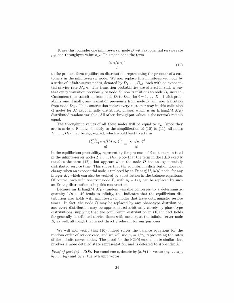
To see this, consider one infinite-server node D with exponential service rateµD and throughput value κD. This node adds the term

(κD/µD)d

d!(12)

to the product-form equilibrium distribution, representing the presence of d cus-tomers in the infinite-server node. We now replace this infinite-server node bya series of infinite-server nodes, denoted by D1, . . . , DM , each with an exponen-tial service rate MµD. The transition probabilities are altered in such a waythat every transition previously to node D, now transitions to node D1 instead.Customers then transition from node Di to Di+1 for i = 1, . . . , D−1 with prob-ability one. Finally, any transition previously from node D, will now transitionfrom node DM . This construction makes every customer stay in this collectionof nodes for M exponentially distributed phases, which is an Erlang(M,Mµ)distributed random variable. All other throughput values in the network remainequal.

The throughput values of all these nodes will be equal to κD (since theyare in series). Finally, similarly to the simplification of (10) to (11), all nodesD1, . . . , DM may be aggregated, which would lead to a term

(∑Mi=1 κD/(MµD))d

d!=

(κD/µD)d

d!

in the equilibrium probability, representing the presence of d customers in totalin the infinite-server nodes D1, . . . , DM . Note that the term in the RHS exactlymatches the term (12), that appears when the node D has an exponentiallydistributed service time. This shows that the equilibrium distribution does notchange when an exponential node is replaced by an Erlang(M,Mµ) node, for anyinteger M , which can also be verified by substitution in the balance equations.Of course, each infinite-server node Bi with µi = 1/τi can be replaced by suchan Erlang distribution using this construction.

Because an Erlang(M,Mµ) random variable converges to a deterministicquantity 1/µ as M tends to infinity, this indicates that the equilibrium dis-tribution also holds with infinite-server nodes that have deterministic servicetimes. In fact, the node D may be replaced by any phase-type distribution,and every distribution may be approximated arbitrarily closely by phase-typedistributions, implying that the equilibrium distribution in (10) in fact holdsfor generally distributed service times with mean τi at the infinite-server nodeBi as well, although that is not directly relevant for our purposes.

We will now verify that (10) indeed solves the balance equations for therandom order of service case, and we will use µi = 1/τi, representing the ratesof the infinite-server nodes. The proof for the FCFS case is quite similar, butinvolves a more detailed state representation, and is deferred to Appendix A.

Proof of part (a) - ROS. For conciseness, denote by (a, b) the vector (a1,. . . , aA,b1, . . . , bB) and by ei the i-th unit vector.

24

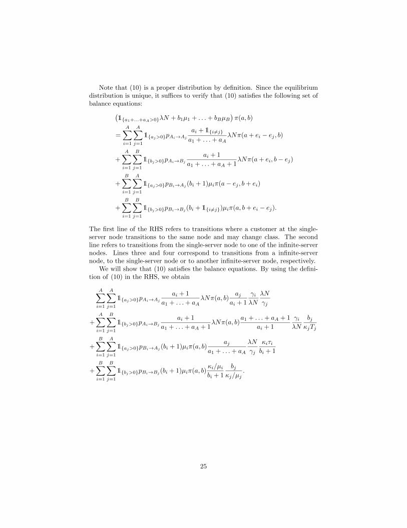
Note that (10) is a proper distribution by definition. Since the equilibriumdistribution is unique, it suffices to verify that (10) satisfies the following set ofbalance equations:(

1{a1+...+aA>0}λN + b1µ1 + . . .+ bBµB)π(a, b)

=

A∑i=1

A∑j=1

1{aj>0}pAi→Aj

ai + 1{i 6=j}

a1 + . . .+ aAλNπ(a+ ei − ej , b)

+

A∑i=1

B∑j=1

1{bj>0}pAi→Bj

ai + 1

a1 + . . .+ aA + 1λNπ(a+ ei, b− ej)

+

B∑i=1

A∑j=1

1{aj>0}pBi→Aj(bi + 1)µiπ(a− ej , b+ ei)

+

B∑i=1

B∑j=1

1{bj>0}pBi→Bj(bi + 1{i 6=j})µiπ(a, b+ ei − ej).

The first line of the RHS refers to transitions where a customer at the single-server node transitions to the same node and may change class. The secondline refers to transitions from the single-server node to one of the infinite-servernodes. Lines three and four correspond to transitions from a infinite-servernode, to the single-server node or to another infinite-server node, respectively.

We will show that (10) satisfies the balance equations. By using the defini-tion of (10) in the RHS, we obtain

A∑i=1

A∑j=1

1{aj>0}pAi→Aj

ai + 1

a1 + . . .+ aAλNπ(a, b)

ajai + 1

γiλN

λN

γj

+

A∑i=1

B∑j=1

1{bj>0}pAi→Bj

ai + 1

a1 + . . .+ aA + 1λNπ(a, b)

a1 + . . .+ aA + 1

ai + 1

γiλN

bjκjTj

+B∑i=1

A∑j=1

1{aj>0}pBi→Aj(bi + 1)µiπ(a, b)

aja1 + . . .+ aA

λN

γj

κiτibi + 1

+

B∑i=1

B∑j=1

1{bj>0}pBi→Bj(bi + 1)µiπ(a, b)

κi/µibi + 1

bjκj/µj

.

25

Next, we combine the inside sums, resulting in

A∑j=1

1{aj>0}aj

a1 + . . .+ aA

λN

γj

[A∑i=1

pA1→Ajγi +

B∑i=1

pBi→Ajκi

]π(a, b)

+

B∑j=1

1{bj>0}bj

κj/µj

[A∑i=1

pAi→Bjγi +

B∑i=1

pBi→Bjκi

]π(a, b)

=

A∑j=1

1{aj>0}aj

a1 + . . .+ aAλN +

B∑j=1

bjµj

π(a, b)

=

1{a1+...+aA>0}λN +B∑j=1

bjµj

π(a, b).

6 Conclusion

We established a universal upper bound for the achievable throughput of anydispatcher-driven algorithm for a given communication budget and queue limit.We also introduced a specific hyper-scalable scheme which can operate at anygiven message rate and enforce any given queue limit, while allowing the systemdynamics to be captured via a closed product-form network. We leveraged theproduct-form distribution to show that the bound is tight, and that the proposedhyper-scalable scheme provides asymptotic optimality in the three-way trade-off among performance, communication and throughput. Extensive simulationexperiments were presented to illustrate the results and make comparisons withvarious alternative design options.

The work-conserving variant covered in Subsection 3.3 is especially worthdiscussing further. Intuitively, letting servers work all the time seems better thanpausing the servers when they become open, but this remains to be rigorouslyproven.

The extension aimed at minimizing waiting times that was introduced inSection 4 warrants further attention as well. For the baseline scenario, wewere able to prove a strict relationship between the amount of communicationand the throughput. Likewise, there might exist a result, similar in spirit toTheorem 1, which provides an upper bound for the throughput and the averagequeue position of admitted jobs, given a certain communication budget. Themain point of concern in this regard is that the concavity argument no longerseems to hold.

Finally, it would be worth investigating whether the current framework couldbe broadened further. It may be possible for example to extend the categoryof algorithms considered, specifically allowing for pull-based schemes. Whilethe results in [7] imply that Theorem 1 does not hold for pull-based schemes,

26

there might be a larger upper bound covering such algorithms as well. Forfurther extensions, other performance metrics might be considered too, such asthe mean waiting time as opposed to the throughput subject to a queue limit.

Acknowledgments

This work is supported by the NWO Gravitation Networks grant 024.002.003and an ERC Starting Grant. We would like to thank Celine Comte and MartinZubeldia for several helpful discussions and suggestions.

References

[1] N. Alon, O. Gurel-Gurevich, and E. Lubetzky. Choice-memory tradeoff inallocations. The Annals of Applied Probability, 20(4):1470–1511, 08 2010.

[2] Jonatha Anselmi and Francois Dufour. Power-of-d-choices with memory:Fluid limit and optimality. Mathematics of Operations Research, 45(3):862–888, 2020.

[3] R. Badonnel and M. Burgess. Dynamic pull-based load balancing for auto-nomic servers. In Network Operations and Management Symposium, 2008.NOMS 2008. IEEE, pages 751–754. IEEE, 2008.

[4] S.A. Berezner, C.F. Kriel, and A.E. Krzesinski. Quasi-reversible multiclassqueues with order independent departure rates. Queueing Systems, 19:345–359, 1995.

[5] M. van der Boor, S.C. Borst, and J.S.H. van Leeuwaarden. Hyper-scalableJSQ with sparse feedback. Proceedings of the ACM on Measurement andAnalysis of Computing Systems, 3(1), March 2019.

[6] M. van der Boor, S.C. Borst, J.S.H. van Leeuwaarden, and D. Mukherjee.Scalable load balancing in networked systems: Universality properties andstochastic coupling methods. In Proceedings of the International Congressof Mathematicians, ICM 2018, volume 4, pages 3911–3942, 01 2018.

[7] M. van der Boor, M. Zubeldia, and S.C. Borst. Zero-wait load balancingwith sparse messaging. Operations Research Letters, 48(3):368–375, 2020.

[8] M. Bramson, Y. Lu, and B. Prabhakar. Randomized load balancing withgeneral service time distributions. In ACM SIGMETRICS PerformanceEvaluation Review, volume 38(1), pages 275–286. ACM, 2010.

[9] M. Bramson, Y. Lu, and B. Prabhakar. Asymptotic independence of queuesunder randomized load balancing. Queueing Systems, 71(3):247–292, 2012.

[10] A. Ephremides, P. Varaiya, and J. Walrand. A simple dynamic routingproblem. IEEE Transactions on Automatic Control, 25(4):690–693, 1980.

27

[11] S.G. Foss and A.L. Stolyar. Large-scale Join-Idle-Queue system with gen-eral service times. Journal of Applied Probability, 54(4):995–1007, 2017.

[12] D. Gamarnik, J.N. Tsitsiklis, and M. Zubeldia. Delay, memory, and mes-saging tradeoffs in distributed service systems. ACM SIGMETRICS Per-formance Evaluation Review, 44(1):1–12, 2016.

[13] R. Gandhi, H.H. Liu, Y.C. Hu, G. Lu, J. Padhye, L. Yuan, and M. Zhang.Duet: Cloud scale load balancing with hardware and software. ACM SIG-COMM Computer Communication Review, 44(4):27–38, 2014.

[14] T. Hellemans and B. Van Houdt. Performance analysis of load balancingpolicies with memory. In Proceedings of the 13th EAI International Confer-ence on Performance Evaluation Methodologies and Tools, VALUETOOLS’20, page 27–34, 2020.

[15] F.P. Kelly. Reversibility and stochastic networks. Cambridge UniversityPress, 2011.

[16] A.E. Krzesinski. Order independent queues. In R. Boucherie , N. van Dijk(eds) Queueing Networks. International Series in Operations Research andManagement Science, volume 154, 2011.

[17] X. Liu and L. Ying. On achieving zero delay with power-of-d-choices loadbalancing. In 2018 IEEE Conference on Computer Communications (IN-FOCOM), pages 297–305, 2018.

[18] Y. Lu, Q. Xie, G. Kliot, A. Geller, J.R. Larus, and A. Greenberg. Join-idle-queue: A novel load balancing algorithm for dynamically scalable webservices. Performance Evaluation, 68(11):1056–1071, 2011.

[19] M.J. Luczak and J.R. Norris. Averaging over fast variables in the fluid limitfor Markov chains: application to the supermarket model with memory.The Annals of Applied Probability, 23(3):957–986, 2013.

[20] S.T. Maguluri, R. Srikant, and L. Ying. Stochastic models of load balancingand scheduling in cloud computing clusters. In 2012 IEEE Conference onComputer Communications (INFOCOM), pages 702–710. IEEE, 2012.

[21] M. Mitzenmacher. How useful is old information? IEEE Transactions onParallel and Distributed Systems, 11(1):6–20, 2000.

[22] M. Mitzenmacher. The power of two choices in randomized load balancing.IEEE Transactions on Parallel and Distributed Systems, 12(10):1094–1104,2001.

[23] M. Mitzenmacher, B. Prabhakar, and D. Shah. Load balancing with mem-ory. In The 43rd Annual IEEE Symposium on Foundations of ComputerScience, 2002. Proceedings., pages 799–808, 2002.

28

[24] D. Mukherjee, S.C. Borst, J.S.H. van Leeuwaarden, and P.A. Whiting. Uni-versality of power-of-d load balancing in many-server systems. StochasticSystems, 8(4):265–292, 2018.

[25] A. Mukhopadhyay, A. Karthik, and R.R. Mazumdar. Randomized assign-ment of jobs to servers in heterogeneous clusters of shared servers for lowdelay. Stochastic Systems, 6(1):90–131, 2016.

[26] A. Mukhopadhyay, A. Karthik, R.R. Mazumdar, and F. Guillemin. Meanfield and propagation of chaos in multi-class heterogeneous loss models.Performance Evaluation, 91:117–131, 2015.

[27] A. Mukhopadhyay and R.R. Mazumdar. Randomized routing schemes forlarge processor sharing systems with multiple service rates. In ACM SIG-METRICS Performance Evaluation Review, volume 42(1), pages 555–556.ACM, 2014.

[28] P. Patel, D. Bansal, L. Yuan, A. Murthy, A. Greenberg, D.A. Maltz,R. Kern, H. Kumar, M. Zikos, H. Wu, K. Changhoon, and N. Karri.Ananta: Cloud scale load balancing. ACM SIGCOMM Computer Com-munication Review, 43(4):207–218, 2013.

[29] A.L. Stolyar. Pull-based load distribution in large-scale heterogeneous ser-vice systems. Queueing Systems, 80(4):341–361, 2015.

[30] N.D. Vvedenskaya, R.L. Dobrushin, and F.I. Karpelevich. Queueing systemwith selection of the shortest of two queues: An asymptotic approach.Problemy Peredachi Informatsii, 32(1):20–34, 1996.

[31] W. Winston. Optimality of the shortest line discipline. Journal of AppliedProbability, 14(1):181–189, 1977.

[32] Q. Xie, X. Dong, Y. Lu, and R. Srikant. Power of d choices for large-scalebin packing: A loss model. ACM SIGMETRICS Performance EvaluationReview, 43(1):321–334, 2015.

[33] L. Ying, R. Srikant, and X. Kang. The power of slightly more than one sam-ple in randomized load balancing. In 2015 IEEE Conference on ComputerCommunications (INFOCOM), pages 1131–1139. IEEE, 2015.

[34] Xingyu Zhou, Fei Wu, Jian Tan, Yin Sun, and Ness Shroff. Designing low-complexity heavy-traffic delay-optimal load balancing schemes: Theory toalgorithms. Proc. ACM Meas. Anal. Comput. Syst., 1(2):39, 2017.

A Proof of Proposition 4 - FCFS case

Proof of part (a) - FCFS. The proof for the FCFS case consists of multiplesteps. First we define a more detailed state space. A state is representedby (c, b) = ((c1, . . . , cm), (b1, . . . , bB)), which represents the situation where m

29

customers are at the single-server node, and the order of the classes of cus-tomers is saved as well: the kth customer at the single-server node has classck. We will sometimes refer to the number of customers of a specific class withai =

∑j 1{cj=Ai}. Furthermore, bi customers are at the infinite-server node Bi.

Equilibrium distribution for the extended state space. We will show that theequilibrium distribution (modulo normalization constant) of state (c, b) equals

π(c, b) =( γ1λN

)a1· · ·( γAλN

)aA (κ1/µ1)b1

b1!· · · (κB/µB)bB

bB !(13)

with ak the number of customers of class Ak.We assume FCFS arrivals of customers at the single-server node: customers

arrive at the end of the line at the single-server node and only the customer firstin line is able to transition.

Balance equations. First, we introduce the balance equations, in which thesymbol m is used to denote the length of vector c,(

1{m>0}λN + b1µ1 + . . .+ bBµB)π(c, b)

=

A∑i=1

1{m>0}pAi→cmλNπ((Ai, c1, . . . , cm−1), b)

+

A∑i=1

B∑j=1

1{bj>0}pAi→BjλNπ((Ai, c1, . . . , cm), b− ej)

+

B∑i=1

1{m>0}pBi→cm(bi + 1)µiπ((c1, . . . , cm−1), b+ ei)

+

B∑i=1

B∑j=1

1{bj>0}pBi→Bj (bi + 1{i 6=j})µiπ(c, b+ ei − ej).

(14)

The term before π(c, b) on the LHS represents the outgoing rate of state (c, b),which equals a rate of λN for the single-server node (if at least one customer ispresent there) plus a rate of bjµj , for each infinite-server node Bj .

On the RHS, four possible transitions to state (c, b) are shown preceded bythe rate of the transitions. First, a transition from the non-empty single-servernode makes the then first customer change its class from cm−1 to class cm. Ifthe previous class order at the single-server node is cm − 1, c1, . . . , cm−1, thena transition to that node will make the class order exactly c. Second, if theprevious class order at the single-server node is K − 1, c1, . . . , cm, then a transi-tion from that node to a infinite-server node will make the class order exactly c.Additionally, if the number of customers at infinite-server node Bj was bj − 1,then it will become bj as the infinite-server node receives an extra customer.Third, any of the customers at the infinite-server nodes might transition to thesingle-server node. Finally, customers might transition from and to one of theinfinite-server nodes.

30

We will show that π satisfies the balance equations. By using the definitionof π in the RHS, we obtain

A∑i=1

1{m>0}pAi→cmλNπ(c, b)γiλN

λN

γcm

+

A∑i=1

B∑j=1

1{bj>0}pAi→BjλNπ(c, b)

γiλN

bjκjτj

+

B∑i=1

1{m>0}pBi→cm(bi + 1)µiπ(c, b)λN

γcm

κi/µibi + 1

+

B∑i=1

B∑j=1

1{bj>0}pBi→Bj(bi + 1)µiπ(c, b)

κi/µibi + 1

bjκj/µj

.

(15)

Next, we reorganize terms, yielding

1{m>0}λN

γcmπ(c, b)

[A∑i=1

pAi→cmγi +

B∑i=1

pBi→cmκi

]

+

B∑j=1

1{bj>0}bj

κj/µjπ(c, b)

[A∑i=1

pAi→Bjγi +

B∑i=1

pBi→Bjκi

]

=

1{m>0}λN +

B∑j=1

bjµj

π(c, b),

(16)

which shows that π is the equilibrium distribution of the extended state space.Finally, note that in the original state space, only the number of customers of

certain classes is tracked. Thus, π(a, b) is an enumeration of π(c, b) over all pos-sible orders with the correct number of customers of a certain class. The numberof possible orders is

(a1+...+aAa1...aA

), which leads to π(a, b) =

(a1+...+aAa1...aA

)π(c, b); the

description of π as presented in the statement of the proposition.

31