Openness, competition, technology and FDI spillovers: Evidence from Romania

Openness, competition, technology and FDIspillovers: Evidence from Romania

Bruno MerlevedeKoen Schoors

Department of Economics and CERISE,

Centre for Russian International Socio-Political and Economic Studies,

Ghent University,

Hoveniersberg 24, B-9000 Ghent, Belgium

[email protected], [email protected]

February 10, 2009

Abstract

We study whether FDI spillovers depend on openness, competitionand the level of technology in a sample of Romanian manufacturing �rms.Spillovers depend on the level of technology in non-linear way and aremore likely to be positive in open sectors than in closed sectors. Hori-zontal spillovers are especially bene�cial export-oriented and competitivesectors. Backward spillovers are very positive for �rms that face globalizedcompetition on their home and export markets, in line with Rodriguez-Clare (1996). Forward spillovers are especially important for �rms thatface high levels of import penetration in their product markets

JEL Classi�cation:Keywords: foreign direct investment, spillovers, absorptive capability

1

1 Introduction

When a �rm invests in a foreign country, it often brings with it proprietary

technology to compete successfully with indigenous �rms (Markusen, 1995).

Believing that this transferred technology will be adopted by domestic �rms,

host country policymakers may try to implement policies to attract foreign di-

rect investment (FDI). Unfortunately, such faith in the positive spillover e¤ects

of FDI contrasts starkly with the empirical evidence (Rodrik, 1999). The liter-

ature surveys of Görg and Greenaway (2004), Smarzynska Javorcik (2004), and

Crespo and Fontoura (2007) conclude that there is no clear evidence of aggre-

gate positive spillovers from FDI. The literature distinguishes spillovers to �rms

in the same industries (intra-industry or horizontal spillovers) and spillovers

to �rms in linked industries (inter-industry or vertical spillovers). Horizontal

spillovers have received widespread attention, while the vertical spillover discus-

sion launched by McAleese and McDonald (1978) and Lall (1980) languished

for two decades until its recent revival by Schoors and van der Tol (2002) and

Smarzynska Javorcik (2004). Schoors and van der Tol (2002) and Smarzyn-

ska Javorcik (2004) distinguish vertical spillovers that occur through contacts

between foreign �rms and their local suppliers in upstream industries (back-

ward spillovers) from those that occur through contacts between foreign �rms

and their downstream customers (forward spillovers). Both studies suggest that

spillovers between industries dominate spillovers within industries. Several pa-

pers in this line of research that aim at identifying vertical spillovers. Kugler

(2006) �nds evidence in a sample of Colombian manufacturing �rms for the

propagation of technology between industries, suggesting that MNCs outsourc-

ing relationships with local upstream suppliers are the main channel of di¤usion.

Gorodnichenko et al. (2007) �nd for a sample of �rms in 17 Central and East-

ern European countries that backward spillovers (stemming from supplying a

foreign �rm in the host country or exporting to a foreign �rm) are consistently

positive.

Our contribution is threefold. First we consider non-linear inter-industry

spillover e¤ects that depend on the level of technology. Second, we classify

sectors along three lines, -import penetration, export orientation and sectoral

competition -, and verify whether FDI spillovers depend on this sector classi-

�cation. Last, we consider the welfare impact of the spillovers implied by our

model. We analyze the spillover e¤ects of FDI in a sample of domestic Romanian

manufacturing �rms. Romania is a good testing ground for the spillover e¤ects

2

Table 1: Overview of spillovers

from FDI, because it received hardly any FDI in the years before the �rst year

of our data sample, 1998, while it received a considerable amount during the

years of our sample. The fact that there is no important stock of FDI before the

period of study allows a clean identi�cation of the spillover e¤ects of interest.

We �nd that vertical spillovers are economically more important than horizontal

spillovers. The spillovers are often found to be dependent on the original level of

technology and on the characteristics of the sector. The welfare e¤ects are found

to be considerable, which underlines the economic signi�cance of FDI spillovers.

In section 2, we provide a short overview of the spillover literature. Section 3

lays out the data and the estimation strategy. Results and interpretation are

provided in section 4. Section 5 concludes.

2 Spillovers of foreign investment to local �rm

productivity

2.1 Direct and indirect e¤ects

Figure 1 illustrates how the spillovers from foreign direct investment run through

the host economy�s production chain.

Horizontal spillovers run from a foreign �rm to a host country �rm in the

same industry. Teece (1977) suggests two main channels for horizontal spillovers:

technology imitation (the demonstration e¤ect) and mobility of workers trained

by foreign �rms (see Fosfuri et al., 2001, and Görg and Strobl, 2005). Marin

and Bell (2006) �nd that training activities by foreign subsidiaries are related

to higher horizontal spillovers. Foreign entry may also fuel competition in the

domestic market. Fiercer competition urges host country �rms to either use

existing technologies and resources more e¢ ciently or adopt new technologies

and organizational practices, which provides another important channel of hor-

izontal spillovers (see Aitken and Harrison, 1999, and Glass and Saggi, 2002).

None of these e¤ects is necessarily positive, however. Labor market dynamics

may entail negative spillovers such as a brain drain of local talent to foreign

�rms to the detriment of local �rm productivity (Blalock and Gertler, 2004) or

an overall increase in wages irrespective of productivity improvements caused

3

final goods

raw materials

# Foreign# Domestic # Domestic

Sector AHorizontal spillover

Forwardspillover

(δAB)

Sector BSector C

Sector DSector E

Backwardspillover

(αAE)

Forwardspillover

(δAC)

Backwardspillover

(αAD)

SpilloverGoods flow

Figure 1: Spillovers through the host economy�s production chain

4

by foreign �rms paying higher wages (Aitken et al., 1996). Where foreign tech-

nology is easily copied, the foreign investor may choose to avoid leakage costs on

state-of-the-art technology by restricting its technology transfer to technology

that is only marginally superior to technology found in the host country (see

Glass and Saggi, 1998). Such policies obviously limit the scope for horizontal

spillovers via demonstration e¤ects. The higher productivity of foreign a¢ liates

may also lead to lower prices or less demand for the products of domestic com-

petitors. If domestic �rms fail to raise productivity in response to the increased

competition, they will be pushed up their average cost curves. Ultimately, do-

mestic producers may not merely fall behind, but fall by the wayside, driven

out of business by the shock of foreign entry (see Aitken and Harrison, 1999, on

this market-stealing e¤ect). These partial e¤ects are hard to disentangle empir-

ically. We identify labor market spillovers by including a measure that accounts

for labor market e¤ects next to a measure that incorporates the net e¤ect of all

other spillovers.

As seen from the top panel in Figure 1, backward spillovers go from the

foreign �rm to its upstream local suppliers. Thus, even if foreign �rms attempt

to minimize their technology leakage to direct competitors (horizontal e¤ect),

they may still want to assist their local suppliers in providing inputs of su¢ cient

quality in order to realize the full bene�ts of their investment. In other words,

they want the inputs from the host country to be lower cost yet similar in quality

to inputs in the home country. If the foreign �rm decides to source locally, it may

transfer technology to more than one domestic supplier and encourage upstream

technology di¤usion to circumvent a hold-up problem. Rodriguez-Clare (1996)

shows that the backward linkage e¤ect is more likely to be favorable when the

good produced by the foreign �rm uses intermediate goods intensively and when

the home and host countries are similar in terms of the variety of intermediate

goods produced. Under reversed conditions, the backward linkage e¤ect could

even damage the host country�s economy. Figure 1 also suggests how a forward

spillover goes from the foreign �rm to its downstream local buyer of inputs. The

availability of better inputs due to foreign investment enhances the productivity

of �rms that use these inputs. However, there is also a danger that inputs

produced locally by foreign �rms are more expensive and less adapted to local

requirements. In this case there would be a negative forward spillover.

5

2.2 The level of technology and non-linear spillovers

The existence, direction, and magnitude of spillovers may depend on the �rm-

speci�c level of technology. Findlay (1978) constructs a dynamic model of tech-

nology transfer through FDI from developed to developing countries. He argues

that there is a positive connection between the distance to the world�s techno-

logical frontier and economic growth. Findlay�s model implies that productivity

spillovers are an increasing function of the technology gap between foreign and

domestic �rms. Acemoglu et al. (2002) and Aghion et al. (2005) on the other

hand use a Schumpeterian model to predict that �rms that are close to the e¢ -

ciency frontier bene�t more from foreign presence than �rms that are far from

the frontier. This is the absorptive capability hypothesis. Kokko et al. (1996)

�nd a positive spillover e¤ect in a subsample of �rms with high absorptive capa-

bility and no e¤ect in a subsample of �rms with low absorptive capability. While

Findlay suggests that spillovers are a negative function of the level of technology,

the absorptive capability interpretation suggests a positive relation. Figure 2

suggests roughly how these competing hypotheses might give rise to non-linear

relationships. In line with these competing hypotheses, Girma and Görg (2005)

o¤er a U-shaped relationship between productivity growth and their horizontal

spillover variable interacted with the level of technology. Girma (2005) observes

that horizontal spillovers increase with absorptive capability up to a threshold

level, beyond which the increase is much less pronounced.

.

2.3 Characteristics of the sector

The existence, direction, and magnitude of spillovers may also depend on sec-

toral characteristics like openness or competition. Domestic �rms in export-

oriented sectors are more likely to be already exposed to contacts with foreign

�rms, new technologies and high competition on their export markets, prior

to the entry of the MNC. This implies that domestic �rms have less to learn

from foreign entrants, but also that they have a greater capacity to absorb the

foreign technology that remains to be learned, as suggested by the results of

Barrios and Strobl (2002) and Schoors and van der Tol (2002) and Sisani and

Meyer (2004). As regards import penetration, Sjöholm (1999) �nds for Indone-

sian �rms that domestic competition rather than competition from imported

goods a¤ects FDI spillovers. The theoretical literature is inconclusive as to the

impact of competition on productivity. Stephen J. Nickell (1996) �nds a posi-

6

Level oftechnology

Spillover effecton firm

productivity

scope forspillover

ability to takeadvantage of

spillover

Level oftechnology

Spillover effecton firm

productivity scope forspillover

ability to takeadvantage of

spillover

Figure 2: Spillovers as a non-linear function of the level of technology

7

tive impact of competition on �rm performance. Wang and Blomström (1992)

are the �rst to stress the importance of competition for FDI spillovers. Higher

levels of competition force foreign subsidiaries to bring relatively new and so-

phisticated technologies from the parent company, which magni�es the potential

for spillovers. The reverse reasoning also applies and reinforces the argument.

Kokko (1994, 1996) examined the e¤ect of FDI on productivity in di¤erent man-

ufacturing sectors. A high technology gap in combination with a low degree of

competition was found to prevent spillovers. There is however a serious identi�-

cation problem in examining productivity levels, as foreign �rms may locate in

highly productive sectors. Nickell (1996) �nds evidence of a generally positive

impact of competition on productivity growth in his empirical analysis. Sjöholm

(1999) �nds in an Indonesian dataset that high sectoral competition (measured

by a Her�ndahl index) raises the magnitude of FDI spillovers, suggesting that

the degree of competition a¤ects the choice of technology transferred to the

MNC�s a¢ liate, and the potential for spillovers size. The literature also con-

siders other conditionalities like the degree of foreign ownership (Blomström

and Sjöholm, 1999; Smarzynska and Spatareanu, 2008) or �rm size, (Sisani and

Meyer, 2004; Merlevede and Schoors, 2008), but these fall beyond the scope of

this contribution.

3 Empirical approach, data, and variables

3.1 Empirical approach

We use a two-step procedure. The �rst step consists in the estimation of a

standard production function. The second step relates the estimated total factor

productivity to measures of FDI spillovers and several control variables.

Our initial problem is that researchers cannot directly observe how �rms re-

act to �rm-speci�c productivity shocks. For example, a �rm confronted with a

large positive productivity shock might respond by using more inputs. Griliches

and Mairesse (1995) provide a detailed account of this problem and make the

case that inputs should be treated as endogenous variables since they are cho-

sen on the basis of the �rm�s, rather than an econometrician�s, assessment of

its productivity. OLS estimates of production functions therefore yield biased

estimates of factor shares and biased estimates of productivity.1 We thus em-

1Speci�cally, the coe¢ cient of labor is biased upwards, while the capital coe¢ cient is biaseddownwards.

8

ploy the semi-parametric approach suggested by Olley and Pakes (1996) and

subsequently modi�ed by James Levinsohn and Amil Petrin (2003).that in-

corporates idiosyncratic shocks to �rm-speci�c productivity di¤erences.� We

estimate domestic industry production functions for each industry j in the pe-

riod 1998�2001, excluding foreign �rms from the estimation. A measure of total

factor productivity tfpit is obtained as the di¤erence between value added and

capital and labor inputs, multiplied by their estimated coe¢ cients:

8j : tfpit = vait � b�llit � b�kkit (1)

In the second step, we relate tfpijrt to a vector of spillover variables, FDI,

a concentration index, H, and industry, region, and time dummies (�j , �r, and

�t). Note that we pool industries for the estimation of (2), whereas (1) is an

industry-speci�c estimation.

tfpijrt = �i +1f (FDIjt; Tijrt)0+ �j + �r + �t + "ijrt (2)

The vector of spillover variables (FDIjt) covers di¤erent transformations of

the horizontal and vertical spillovers. We interact our three spillover variables

(horizontal, backward, forward) with the �rm-speci�c level of technology (Tijrt)

in a non-linear way. Speci�cation (2) is �rst di¤erenced and estimated as a �xed

e¤ects model:

�tfpijrt = �i +1�f (FDIjt; Tijrt)0+ �t + "ijrt (3)

The �xed e¤ects control for all time-invariant �rm-speci�c unobservables

driving productivity growth, including region and industry e¤ects. The �rst-

di¤erenced time dummies still control for the business cycle. Because FDIjtand Hjt are de�ned at the industry level, while estimations are performed at

the �rm level, standard errors need to be adjusted (see Brent R. Moulton,

1990). Standard errors are clustered for all observations in the same industry

and year. The e¤ects of openness and competition are considered by estimating

(3) for di¤erent subsamples. First we consider the characteristics separately

(high versus low export share, high versus low import penetration, high versus

low competition). In a second phase we consider these characteristics jointly,

by running (3) for 8 exclusive subsamples that cover all possible combinations

of the three characteristics of interest.

9

3.2 Data description and variable de�nitions

Romanian �rm-level data for 1996�2001 are drawn from the Amadeus database

published on DVD and CD by Bureau Van Dijk. Given our interest in import

penetration and export orientation we limit our sample to manufacturing �rms.

Other sectors are largely producing non-tradables and their inclusion would ob-

fuscate the distinction between closed sectors and service sectors. The sample is

unbalanced due to �rms entering in later years. There is no �rm exit. Industry

price level data at Nace 2-digit level2 are taken from the Industrial Database for

Eastern Europe from the Vienna Institute for International Economic Studies

and from the Statistical Yearbook of the Romanian National Statistical O¢ ce

(RNSO). Our industry classi�cation follows the classi�cation used in the Ro-

manian input-output (IO) tables. This classi�cation is then linked to the Nace

classi�cation scheme. The entire Amadeus series is used to construct a database

of time-speci�c foreign entry in local Romanian �rms.3 IO tables for the period

1995�2001 were obtained from the RNSO.

The matrix FDI in (3) contains measures of foreign presence to capture the

di¤erent spillovers described above. We classify a �rm as foreign (Foreign =

1) when foreign participation exceeds 10%.4 The horizontal spillover variable

Horizontaljt captures the degree of foreign presence in sector j at time t and

is measured as industry j�s share of output produced by foreign-owned �rms:

Horizontaljt =

Pi2j Foreignit � YitP

i2j Xit(4)

For the measurement of the backward spillover variable Backwardjt, one

possibility might be to employ the share of �rm output sold to foreign �rms.

However, this information is unavailable from our dataset. Moreover, the share

of �rm output sold to foreign-owned domestic �rms may cause endogeneity

problems if the latter prefer to buy inputs from more productive domestic �rms.

2Nomenclature générale des activités économiques dans les Communautés européennes.3Amadeus DVDs are released each year. They provide a pan-European database of �nancial

information on public and private companies. Speci�c entries, however, only indicate the mostrecent ownership information. Since ownership information is gathered at irregular intervals,we do not have ownership information for all years and �rms. Ownership changes tend toshow up ex post in the database. Therefore, if a given �rm has any gaps in its ownershipseries, we �ll the gaps with the information from the following year.

4This threshold level is commonly applied (e.g. by the OECD) in FDI de�nitions.

10

We thus measure Backwardjt as :

Backwardjt =X

k if k 6=j jkt �Horizontalkt (5)

where jkt is the proportion of industry j�s output supplied to sourcing industry

k at time t. The s are calculated from the time-varying IO tables for interme-

diate consumption. Horizontalkt is a measure for foreign presence in industry

k at time t. In the calculation of , we explicitly exclude inputs sold within the

�rm�s industry (k 6= j) because this is captured by Horizontaljt.5 Since �rmscannot easily switch between industries for their inputs, we can avoid the prob-

lem of endogeneity by using the share of industry output sold to downstream

domestic markets with some foreign presence. In the same spirit, we de�ne the

forward spillover variable Forwardjt as:

Forwardjt =X

l if l 6=j�jlt �Horizontallt (6)

where the IO tables reveal the proportion �jlt of industry j�s inputs purchased

from upstream industries l. Inputs purchased within the industry (l 6= j) are

again excluded, since this is already captured by Horizontal.6

A measure of the level of technology needs to re�ect the relative technical

capabilities of a domestic �rm vis-à-vis the foreign �rms in the same industry.

In constructing measure Tit, we apply the Levinsohn-Petrin technique on earlier

years of the full sample of both domestic and foreign �rms to avoid endogeneity.

The estimated relation is then used to derive total factor productivity measures

'it for all �rms. Tit is de�ned in (7) as the distance between �rm i�s lagged

productivity level, 'it�1, and the lagged �foreign frontier�in its industry. The

latter is de�ned as the mean productive e¢ ciency of the 25% most productive

foreign �rms in industry j ('jt�1;FOR). More productive �rms have higher

5To clarify, we o¤er the following example. Consider three sectors: j, k1, and k2. Supposethat half of the output of j is purchased by k1 and the other half by k2. Further suppose thatno foreign �rms are active in k1, but half of the output of k2 is produced by foreign �rms.The backward variable for sector j would be (0:5 � 0:0) + (0:5 � 0:5) = 0:25. From this, itcan be easily seen that the value of Backward increases with foreign presence in the sectors kthat source inputs from j and with the share of output of sector j supplied to industries withforeign presence.

6Consider three sectors: j, l1, and l2. Suppose j buys 75% of its inputs with l1 and theremaining 25% with l2. Further suppose that 10% of l1�s output is produced by foreign �rms,and half of the output of l2 is produced by foreign �rms. The backward variable for sector jwould be (0:75 � 0:10) + (0:25 � 0:50) = 0:20.

11

I III

II IV

V VII

VI VIII

low sectoralcompetition

high sectoralcompetition

high importcompetition

low importcompetition

high exportcompetition

low exportcompetitio

n

5033 (28)

646 (25)

5511 (11)

639 (26)

403 (15) 113 (16)

1725 (20) 1969 (30)

Figure 3: Classi�cation of sectors according to three criteria

values of T .

Tit ='it�1

'jt�1;FOR(7)

3.3 Subamples and summary statistics

We �rst split the sample in subsamples according to levels of export orientation,

import penetration and sectoral competition. Export orientation is measured

by the share of sectoral exports in total sectoral output from the time varying

IO tables. IImport penetration is measured by the share of imports of products,

comparable to the produce of the sector, in total sectoral output from the time

varying IO tables. Sectoral competition is proxied by the Her�ndahl index.

Then we combine these three criteria to classify �rms and sectors into 8 classes

Figure splitsample shows precisely how we split the sample in 8 exclusive

12

subsamples and indicates the number of �rms and sectors (between brackets) in

each subsample. Subample I consists of high export, high import, high competi-

tion sectors (sectors that engage in globalized competition on all markets) . We

have 5033 �rms and 10364 observations in subsample I. Subample II consists of

low export, high import, high competition sectors (sectors that face globalized

competition on their home market). We have 1725 �rms and 3618 observations

in subsample II. Subsample III contains the high export, low import, high com-

petition sectors (sectors with a competitive advantage). We have 5511 �rms and

12310 observations in subsample III. Subsample IV contains the low export, low

import, high competition sectors (closed but locally competitive sectors) We

have 1969 �rms and 4226 observations in subsample IV. Subsample V consists of

high export, high import, low competition sectors (open sectors with high entry

barriers). We have only 646 �rms with 996 �rms in subsample V. Subsample

VI contains low export, high import, low competition sectors (sectors that are

faced with devastating import competition). We have 403 �rms with 602 ob-

servations in subsample VI. Subsample VII consists of high export, low import,

low competition sectors (export-led growth of concentrated industries). We have

639 �rms and 1327 observations in subsample VII. Subsample VIII contains low

export, low import, low competition sectors (closed and unreformed sectors).

insert TABLE 1 around hereTable 1 gives summary statistics for the variables described above. The ta-

ble shows data on real output, real materials, real capital, labor, the level of

technology and the spillover variables of interest. Panel A provide the summary

statistics for the sample splits according to import penetration, export orien-

tation and sectoral competition. Panel B provides the summary statistics for

the eight exclusive classes. The average values for the spillovers are surprisingly

similar across sectors, which ensures that any found di¤erences in spillover ef-

fects are not due to the fact that the level of foreign involvement is di¤erent in

di¤erent types of sectors. This is less surprising in panel A, where the various

columns are not exclusive, than in panel B, where the 8 subclasses are de�ned

as exclusive classes.

4 Results and interpretation

INSERT Table 2 and around hereTable 2 shows how the estimates of (3) depend on import penetration, export

13

orientation and industry concentration. The �rst column shows results for all

observations in the sample. Further columns show split sample results for low

and high import penetration (columns 2 and 3), low and high export orientation

(columns 4 and 5) and low and high competition (columns 6 and 7). Panel A of

table 1 shows the estimates of the linear spillover e¤ects. Only the horizontal

spillovers are found to play a signi�cant role. The signi�cance of all vertical

spillover e¤ects is rejected, with the exception of a positive backward spillover

in the export-oriented sectors, which are already used to supplying foreign �rms.

Panel B reveals that the insigni�cance of most vertical spillovers e¤ects in panel

A is explained by the inappropriate linearity assumed in panel A. Indeed, most

vertical spillovers are now found to be signi�cant. This is supported by the joint

signi�cance F-tests reported in panel C. These tests suggest that horizontal and

backward spillovers are only insigni�cant in sectors that export a low share their

total production. The other spillover e¤ects can no longer be rejected, either in

a linear or a non-linear form. The introduction on non-linear e¤ects also raises

the explanatory power of the regression by about 8% from around 2% in panel

A to about 10%. This suggests by and large that the non-linear interactions

with the level of technology are essential to a good understanding of the nature

of productivity spillovers, as hypothesized.

In table 2 we observe that positive spillovers are more likely if import pen-

etration is high, if export orientation is high and if competition is high than in

the converse cases. Horizontal spillovers for example are consistently positive in

open or competitive sectors (columns 3, 5 and 7), while this is not necessarily or

less the case in closed or less competitive sectors. The found di¤erences across

subsamples suggest that the ambiguous results in the literature about the sign

and the magnitude of horizontal spillovers may be explained by di¤erences in

openness and competition. Another result that catches the eye is that the rela-

tion between backward spillovers and the level of technology mostly shows an

inverted U pattern, with backward spillovers turning less positive or negative at

larger levels of technology,.while the relation between forward spillovers and the

level of technology mostly shows a classical U-pattern, with forward spillovers

more likely to be positive at fairly low levels of technology. For both vertical

spillovers the sectors with low import penetration constitute an exception to

this rule. The non-linear relation of horizontal spillovers with the level of tech-

nology also follows a classical U-shape, but is clearly less pronounced than in

the case of forward spillovers.

INSERT Table 3 and �gure 4 around here

14

Table 3 shows estimates of (3) for the exclusive subclasses de�ned in �gure

3. Since we have only 113 �rms and 199 observations in subsample 8, estimates

are very unstable. Therefore table 3 reports estimates of (3) for the �rst 7 sub-

samples only. The implied non-linear productivity spillover are plotted in �gure

4. With respect to horizontal spillovers Table 3 and Figure 4 rea¢ rm the ear-

lier result that horizontal spillovers are particularly positive in sectors that are

both export-oriented and competitive (subsamples I, III). If we remove the cri-

terion of high export orientation (subsamples II, IV), horizontal spillovers turn

insigni�cant, though still positive . If we remove the criterion of competition

(subsamples V, VII) or both criteria (subsample VI) the horizontal spillovers

turn largely negative, though not always signi�cant. These �ndings are in line

with Wang and Blomström (1992), who �nd low or negative horizontal spillovers

in sectors with low competition, and with Barrios and Strobl (2002), Schoors

and van der Tol (2002) and Sisani and Meyer (2004), who �nd more positive

spillovers in export-oriented industries, but in contrast to Sjöholm (1999), who

�nds that horizontal spillovers are positive in competitive sectors especially if

these sectors are still relatively closed (the so-called demonstration e¤ect).

The results in Table 3 and Figure 4 also suggest that the backward spillover

is very positive for sectors that are engaged in global competition in their home

and export markets (subsample I). This is in line with the model of Rodriguez-

Clare (1996) who shows that backward spillover e¤ects should be positive if the

inputs required are not too di¤erent from the ones already produced by the lo-

cal �rms. This condition is more likely to be ful�lled in export-oriented sectors.

Firms in these sectors are already used to the required quality on export mar-

kets and will more easily adapt to the demand from foreign �rms in downstream

sectors. The impact on productivity will be especially pronounced if import pen-

etration is high (the foreign �rm has an option to buy imported components)

and sectoral competition is high (there is competition between local �rms to

make the components for the foreign �rm). In addition, the backward spillover

is also signi�cantly positive, though economically less important, in sectors with

low competition and import penetration, but still a high degree of export ori-

entation (subsample VII). Clearly, backward spillovers can be very positive in

sectors that pursue a strategy of export-led growth. This is in line with anecdo-

tal evidence of host country suppliers of foreign �rms becoming more productive

and turning into competitors of the home country suppliers, initially on the host

country market and in the long run even on the home country market.

The results also suggest that forward spillovers are not very positive in man-

15

ufacturing sectors. Merlevede and Schoors (2008) �nd that forward spillovers

are very positive if all sectors are considered. It is clear therefore that positive

forward spillovers are mainly to be found in non-tradable and service sectors

(�nancial services, business services, communication, trade, energy) . There is

however one important exception to this general rule: Forward spillovers tend

to be very positive economically and statistically in sectors faced with severe

import competition (low export, low competition, high import, subsample VI).

In these sectors access to better and cheaper inputs is a necessary condition to

cope with import competition. Forward spillovers are self-evidently not very

important for �rms in export-oriented sectors, since these need to produce high

quality anyhow and will have been forced already to buy better foreign inputs

if local input quality were too low. So these �rms can at best only bene�t

marginally from better local inputs.

The analysis above portrays the contribution of the spillovers to TFP as a

function of the �rm�s level of technology at the average values of the spillover

variables. This neither reveals what actually happened to Romanian �rms, nor

provides a sound basis for FDI policy. Since �rms are subject to all spillover

e¤ects at the same time, the correlations between the spillover variables will mat-

ter to determine their eventual economic impact. Moreover, the spillover vari-

ables, their correlation structure, and the �rm�s level of technology change over

the time period considered. To analyze the economic signi�cance of spillover

e¤ects for the domestic Romanian �rms in the period 1998-2001 we use the

results of Table 3, panel B, to calculate the total net e¤ect of foreign presence

on domestic �rms. We predict the contribution to total factor productivity of

the di¤erent spillovers at the �rm level by multiplying the estimated coe¢ cients

with the actual values of the variables concerned.

Figure 5 show the spillovers�contribution to total factor productivity growth

during the period 1998�2001, averaged over all �rms in the subclass. H shows

the accumulated 1998-2001 productivity impact for horizontal spillovers, B for

backward spillovers, F for forward spillovers andP

indicates the sum of all

three spillovers. The results suggest that the eventual economic impact of FDI

spillovers on local �rm productivity is potentially large, but strongly depends on

the characteristics of the sector. The net productivity impact of the spillovers

ranges from 0.626 in subsample I (the high competition, high openness sectors)

to -0.367 in subsample II (sectors that face globalized competition on their home

market). Net spillovers seem to be especially bene�cial in highly competitive,

export-oriented sectors (sector I and III). These are also the only sectors were

16

I III

II IV

V VII

VI VIII

low sectoralcompetition

high sectoralcompetition

high importpenetration

low importpenetration

high exportorientation

low exportorientation

n.a.

H 0.273B 0.256F 0.097∑ 0.626

H 0.001B 0.010F 0.378∑ 0.367

H 0.404B 0.045F 0.079∑ 0.280

H 0.021B 0.025F 0.091∑ 0.045

H 0.012B 0.034F 0.364∑ 0.342

H 0.075B 0.819F 1.213∑ 0.470

H 0.042B 0.171F 0.085∑ 0.214

Figure 4: The spillovers�implied impact on �rm level productivity

17

the horizontal spillover is large and positive. The forward spillover is especially

bene�cial to local �rms of subsample VI. These are the sectors that face sti¤

import competition, without the bene�t of either experience on export markets

or local competition. Apparently the access to better inputs through foreign

investment in these �rms�local supplier sectors, greatly enhances their ability

to face down the import competition. In most other subsamples however, the

forward spillover is either small or negative. The backward spillover on the other

hand is especially detrimental to local �rm productivity in the same subsample

VI. This seems logical: In sectors where imported goods dominate the local

market and threaten to wipe out local �rms, foreign �rms in user sectors will

simply buy imported goods rather then sourcing locally. In the other subsam-

ples, the backward spillovers have either a negligible or a positive e¤ect on local

�rm productivity. In Annex we provide the average contribution of spillovers

to total factor productivity growth during the period 1998�2001 for di¤erent

ranges of the initial level of technology. The breakdown in technology ranges is

based on the 1998 level of technology percentiles.

5 Conclusions

This paper investigates whether productivity spillovers from foreign �rms to

domestic manufacturing �rms depend on the sectoral levels of import penetra-

tion, export orientation and competition. We test this on a comprehensive set

of Romanian manufacturing �rms. In the estimation of the production function

we allow unobserved productivity shocks. In the �nal regressions, productiv-

ity di¤erences are explained by horizontal, backward and forward productivity

spillovers from foreign investment. Here we allow non-linear interactions be-

tween the spillover variables and the �rm-speci�c level of technology.

Spillovers a¤ect productivity in a highly non-linear way. Both horizontal and

vertical spillovers are more likely to be positive in open sectors than in closed

sectors. Horizontal spillovers are most positive in sectors that are both export-

oriented and competitive. They turn insigni�cant or even negative if these

conditions are not met. This result may explain the lack of consensus in the

literature about the direction and magnitude of the e¤ect of horizontal spillovers

on local form productivity. Highly positive backward spillovers are found in

highly competitive and open sectors. The positive backward spillovers in these

sectors characterized by "globalized competition" are in line with Rodriguez-

18

Clare (1996) who shows that backward spillover e¤ects are bene�cial if the inputs

required are not too di¤erent from the ones already produced by the local �rms.

In addition the backward spillover is signi�cantly positive, though economically

less important, in sectors with low competition and import penetration, but still

a high degree of export orientation. This is in line with the narrative that new

local suppliers of foreign �rms may grow to compete with and even outperform

the home-country suppliers of the foreign �rm. Forward spillovers are, as in

most of the literature, not very important for manufacturing �rms, except for

sectors that struggle to cope with very high levels of import penetration in

their product markets. In the latter sectors the access to better and cheaper

inputs through foreign investment in supply sectors helps �rms to compete with

imported produce. The debate in the literature on the direction and magnitude

of spillovers from foreign �rms to local �rms has a fair answer: it all depends

on technology, openness and competition.

19

References

Acemoglu, D., Aghion, P., Zilibotti, F.,2002. Vertical Integration and Distanceto Frontier. Journal of the European Economic Association, Papers andProceedings.

Aghion, P., Bloom, N., Blundell, R.,Gri¢ th, R., Howitt, P., 2005. Competitionand Innovation: An Inverted U Relationship. Quarterly Journal of Eco-nomics 120(2), 701-.

Aitken, B. and A. Harrison, 1999, Do Domestic Firms Bene�t from Direct For-eign Investment? Evidence from Venezuela, American Economic Review,vol. 89(3), pp. 605-18

Aitken, B., A. Harrison and R. Lipsey, 1996, Wages and Foreign Ownership: AComparative Study of Mexico, Venezuela and the United States, Journal ofInternational Economics, vol. 40, pp.345-71

Barrios, S., & Strobl, E., 2002, Foreign direct investment and productiv-ity spillovers: evidence from the Spanish experience. WeltwirtschaftlichesArchiv,138(3), 459�481.

Belderbos, R., Capannelli, G.,

Blalock, G. and P. Gertler, 2004, Firm Capabilities and Technology Adoption:Evidence from Foreign Direct Investment in Indonesia, mimeo

Blomström, M. and A. Kokko, 1998, MNCs and Spillovers, Journal of EconomicSurveys, vol. 12(3), pp. 247-77

Blomström, M. and F. Sjöholm, 1999, Technology Transfer and Spillovers: DoesLocal Participation with Multinationals Matter?, European Economic Re-view, vol. 43, pp. 915-923

Caves, R., 1974, Multinational Firms, Competition and Productivity in Host-Country Markets, Economica, vol. 41(162), pp. 176-93

Cohen, W. and D. Levinthal, 1989, Innovation and Learning: The Two Facesof R&D, The Economic Journal, vol. 99(397), F569-F596

Crespo, N., Fontoura, M.P., 2007. Determinant Factors of FDI Spillovers �WhatDo We Really Know? World Development 35(3), 410�425.

Damijan, J., M. Knell, B. Macjen and M. Rojec, 2003, The role of FDI, R&Daccumulation and trade in transferring technology to transition countries:Evidence from �rm panel data for eight transition countries, Economic Sys-tems, vol. 27(2), pp. 127-153

Damijan, J., M. Knell, B. Macjen and M. Rojec, 2003, Technology Transferthrough FDI in Top-10 Transition Countries: How important are Direct Ef-fects, Horizontal and Vertical Spillovers?, William Davidson Institute Work-ing Paper No. 459, 29p.

20

Djankov, S. and B. Hoekman, 2000, Foreign Investment and ProductivityGrowth in Czech Enterprises, World Bank Economic Review, vol. 14(1),pp. 49-64

Findlay, R., 1978, Relative backwardness, direct foreign investment, and thetransfer of technology: A simple dynamic model, Quarterly Journal of Eco-nomics, vol. 92, pp. 116

Fosfuri, A., M. Motta and T. Rønde, 2001, Foreign Direct Investment andSpillovers through Workers�Mobility, Journal of International Economics,vol. 53(1), pp. 205-22

Frydman, R., C. Gray, M. Hessel and A. Rapaczynski, 1999, When Does Privati-zation Work? The Impact of Private Ownership on Corporate Performancein the Transition Economies, Quarterly Journal of Economics, vol. 114(4),pp. 1153-91

Görg, H. and E. Strobl, 2001, Multinational companies and productivityspillovers: A meta-analysis, Economic Journal, vol. 111, pp. F723-39

Görg, H. and D. Greenaway, 2003, Much ado about nothing? Do domestic �rmsreally bene�t from Foreign Direct Investment?, IZA Discussion Paper No.944, 34p.

Glass, A. and K. Saggi, 1998, International Technology Transfer and the Tech-nology Gap, Journal of Development Economics, vol. 55, pp. 369-98

Glass, A. and K. Saggi, 2002, Multinational Firms and Technology Transfer,Scandinavian Journal of Economics, vol. 104(4), pp. 495-513

Globerman, S., 1979, Foreign Direct Investment and Spillover E¢ ciency Bene�tsin Canadian Manufacturing Industries, Canadian Journal of Economics,vol. 12(1), pp. 42-56

Gri¢ th, R., 1999, Using the ADR Establishment Level Data to Look at theForeign Ownership and Productivity in the United Kingdom, EconomicJournal, vol. 109(456), pp. F416-41

Griliches, Z. and J. Mairesse, 1995, Production Functions: The Search for Iden-ti�cation, NBER Working Paper No. 5067, 40 p.

Harris, R. and C. Robinson, 2002, The E¤ect of Foreign Acquisitions on TotalFactor Productivity: Plant-Level Evidence from UK Manufacturing, 1987-1992, The Review of Economics and Statistics, vol. 84(3), pp. 562-68

Haskel, J., S. Pereira and M. Slaughter, 2002, Does Inward Foreign Direct In-vestment Boost the Productivity of Domestic Firms, NBER Working PaperNo. 8724, 38p.

Kinoshita, Y., 2001, R&D and Technology Spillovers through FDI: Innovationand Absorptive Capacity, CEPR Discussion Paper No. 2775

21

Kokko, A., 1994, Technology, Market Characteristics, and Spillovers, Journal ofDevelopment Economics, vol. 43, pp. 279-93

Kokko, A., 1996, Productivity Spillovers from Competition between Local Firmsand Foreign A¢ liates, Journal of International Development, vol. 8, pp.517-30

Kokko, A., R. Tansini and M. Zejan, 1996, Local Technological Capability andProductivity Spillovers from FDI in the Uruguayan Manufacturing Sector,The Journal of Development Studies, vol. 32(4), pp. 602-11

Konings, J., 2001, The E¤ects of Foreign Direct Investment on Domestic Firms- Evidence from Firm-Level Panel Data in Emerging Economies, Economicsof Transition, vol. 9(3), pp. 619-33

Lall, S., 1980, Vertical Inter�rm Linkages in LDCs: An Empirical Study, OxfordBulletin of Economics and Statistics, vol. 42, pp. 203-26

Leahy, D. and P. Neary, 2004, Absorptive Capacity, R&D Spillovers and PublicPolicy, CEPR Discussion Paper No. 4171

Levinsohn, J. and A. Petrin, 2003, Estimating Production Functions Using In-puts to Control for Unobservables, Review of Economic Studies, Vol. 70,pp. 317-41

Liu, X., Siler, P., Wang, C. and Y. Wei, 2000, Productivity spillovers fromForeign Direct Investment: Evidence from UK Industry Level Panel Data,Journal of International Business Studies, vol. 31(3), pp.407-425

McAleese, D. and D. McDonald, 1978, Employment Growth and Development ofLinkages in Foreign-owned and Domestic Manufacturing Enterprises, OxfordBulletin of Economics and Statistics, vol. 40, pp. 321-39

Nickell, S., 1996, Competition and Corporate Performance, Journal of PoliticalEconomy, vol. 104(4), pp. 724-46

Olley, G. and A. Pakes, 1996, The Dynamics of Productivity in the Telecom-munications Equipment Industry, Econometrica, Vol. 64(6), pp. 1263-97

Pack., H. and K. Saggi, 2001, Vertical Technology Transfer via InternationalOutsourcing, Journal of Development Economics, vol. 65, pp. 389-415

Petrin, A., B. Poi and J. Levinsohn, 2004, Production Function Estimation inStata Using Inputs to Control for Unobservables, The Stata Journal, vol.4(2), pp. 113-23

Rodríguez-Clare, A., 1996, Multinationals, Linkages, and Economic Develop-ment, American Economic Review, vol. 86(4), pp. 852-73

22

Rodrik, D., 1999, The New Global Economy and Developing Countries: MakingOpenness work, Overseas Development Council (Baltimore, MD), PolicyEssay No. 24.

Sabirianova Peter, K., J. Svejnar and K. Terell, 2004, Distance to the E¢ ciencyFrontier and FDI Spillovers, forthcoming in Journal of the European Eco-nomic Association Papers and Proceedings

Schoors, K. and B. Van Der Tol, 2002, Foreign Direct Investment Spilloverswithin and between Sectors: Evidence from Hungarian Data, Ghent Uni-versity Working Paper 02/157, available on line

Sinani, E. and K. Meyer, 2004, Spillovers of technology transfer from FDI: Thecase of Estonia, Journal of Comparative Economics, vol. 32, pp. 445-66

Sjöholm, F., 1999, Technology Gap, Competition and Spillovers from ForeignDirect Investment: Evidence from Establishment Data, Journal of Devel-opment Studies, vol. 36(1), pp. 53-73

Smarzynska Javorcik, B., 2004, Does Foreign Direct Investment Increase theProductivity of Domestic Firms? In Search of Spillovers Through BackwardLinkages, American Economic Review, Vol. 94(3), pp.605-27

Smarzynska Javorcik, B. and M. Spatareanu, 2008, To Share or not to Share:Does Local Participation Matter for Spillovers from Foreign Direct Invest-ment, Journal of Development Economics, 85 (1-2), pp. 194-217.

Teece, D. (1977), Technology Transfer by Multinational Firms: The ResourceCost of Transferring Technological Know-how, Economic Journal, vol. 87,pp. 242-61

Wang, J. and M. Blomström, 1992, Foreign Investment and Technology Trans-fer: A Simple Model, European Economic Review, vol. 36, pp. 137-55

Yudaeva, K., K. Kozlov, N. Melentieva and N. Ponomareva, 2003, Does For-eign Ownership Matter? Russian Experience, Economics of Transition, vol.11(3), pp. 383-410

Zukowska-Gagelmann, K., Productivity Spillovers From Foreign Direct Invest-ment In Poland,Economic Systems, vol. 24(3)

23

24

Table 1 Summary Statistics Panel A Summary statistics for the three sample splits

All firms Low import penetration

High import penetration

Low export orientation

High export orientation

Low competition

High competition

Ln(real output) 9.56 9.41 9.74 9.73 9.50 9.89 9.52 (1.99) (1.92) (2.05) (1.93) (2.00) (2.16) (1.96) Ln(labour) 2.15 2.09 2.22 2.01 2.20 2.38 2.13 (1.58) (1.51) (1.66) (1.50) (1.61) (1.84) (1.55) Ln(real capital) 7.63 7.51 7.77 7.80 7.57 8.00 7.59 (2.51) (2.41) (2.61) (2.43) (2.54) (2.76) (2.48) Ln(real materials) 8.80 8.63 9.00 9.01 8.74 9.12 8.77 (2.17) (2.10) (2.23) (2.14) (2.18) (2.35) (2.15) T 0.19 0.18 0.21 0.21 0.18 0.22 0.19 (0.19) (0.18) (0.20) (0.21) (0.19) (0.22) (0.19) Horizontal 0.24 0.24 0.25 0.24 0.25 0.24 0.24 (0.10) (0.09) (0.12) (0.11) (0.10) (0.19) (0.09) Backward 0.23 0.22 0.24 0.24 0.23 0.22 0.23 (0.05) (0.05) (0.04) (0.05) (0.05) (0.05) (0.05) Forward 0.26 0.26 0.27 0.28 0.26 0.24 0.27 (0.07) (0.05) (0.08) (0.06) (0.07) (0.05) (0.07) # of observations 33642 18062 15580 8645 24997 3124 30518

25

Panel B Summary statistics for the sector classifications

All firms I II III IV V VI VII VIII Ln(real output) 9.56 9.65 9.84 9.30 9.59 10.16 9.79 9.65 10.41 (1.99) (2.03) (2.06) (1.92) (1.78) (2.14) (2.03) (2.21) (1.95) Ln(labour) 2.15 2.25 2.07 2.11 1.93 2.53 2.04 2.43 2.25 (1.58) (1.64) (1.64) (1.49) (1.37) (1.95) (1.51) (1.94) (1.38) Ln(real capital) 7.63 7.67 7.89 7.40 7.70 8.32 7.82 7.78 8.47 (2.51) (2.57) (2.62) (2.43) (2.22) (2.83) (2.67) (2.80) (2.17) Ln(real materials) 8.80 8.90 9.18 8.54 8.79 9.36 9.18 8.80 9.94 (2.17) (2.21) (2.25) (2.09) (2.00) (2.29) (2.21) (2.44) (2.10) T 0.19 0.19 0.24 0.17 0.19 0.25 0.17 0.22 0.17 (0.19) (0.19) (0.22) (0.17) (0.20) (0.24) (0.20) (0.22) (0.20) Horizontal 0.24 0.25 0.24 0.25 0.21 0.20 0.36 0.21 0.22 (0.10) (0.10) (0.12) (0.08) (0.06) (0.15) (0.23) (0.17) (0.06) Backward 0.23 0.24 0.24 0.22 0.24 0.21 0.24 0.22 0.23 (0.05) (0.04) (0.05) (0.05) (0.06) (0.04) (0.04) (0.06) (0.03) Forward 0.26 0.27 0.27 0.25 0.29 0.25 0.24 0.24 0.23 (0.07) (0.09) (0.05) (0.04) (0.06) (0.04) (0.05) (0.05) (0.05) # of observations 33642 10364 3618 12310 4226 996 602 1327 199

26

Table 2 Panel A Are simple spillovers dependent on sector characteristics?





Low competition

High competition

ΔHorizontal 1.385*** 1.414*** 4.113*** 1.986** 1.341*** 0.336* 5.198*** [0.471] [0.357] [1.019] [0.931] [0.507] [0.197] [1.132] ΔBackward 1.114** 0.612 1.297 0.575 2.255** 0.790 0.515 [0.492] [0.647] [0.850] [0.370] [1.140] [0.621] [0.537] ΔForward -0.544 -0.815 -0.066 -2.144 -0.308 -0.290 0.108 [0.514] [1.476] [0.561] [1.362] [0.492] [0.851] [0.551] # observations 33642 18062 15580 8645 24997 3124 30518 # firms 15011 8220 7326 3898 11418 1409 13817 R-squared 0.02 0.02 0.04 0.04 0.02 0.07 0.03

27

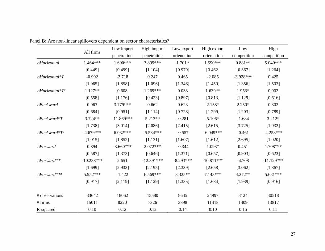
Panel B: Are non-linear spillovers dependent on sector characteristics?





Low competition

High competition

ΔHorizontal 1.464*** 1.600*** 3.899*** 1.701* 1.590*** 0.881** 5.040*** [0.449] [0.499] [1.104] [0.979] [0.462] [0.367] [1.264] ΔHorizontal*T -0.902 -2.718 0.247 0.465 -2.085 -3.928*** 0.425 [1.065] [1.858] [1.096] [1.346] [1.450] [1.356] [1.503] ΔHorizontal*T² 1.127** 0.608 1.269*** 0.033 1.639** 1.953* 0.902 [0.558] [1.176] [0.423] [0.897] [0.813] [1.129] [0.616] ΔBackward 0.963 3.779*** 0.662 0.623 2.158* 2.250* 0.302 [0.684] [0.951] [1.114] [0.728] [1.299] [1.203] [0.789] ΔBackward*T 3.724** -11.869*** 5.213** -0.281 5.106* -1.684 3.212* [1.738] [3.014] [2.086] [2.415] [2.615] [3.725] [1.932] ΔBackward*T² -4.679*** 6.032*** -5.534*** -0.557 -6.049*** -0.461 -4.258*** [1.015] [1.852] [1.131] [1.607] [1.612] [2.695] [1.020] ΔForward 0.894 -3.660*** 2.072*** -0.344 1.093* 0.451 1.708*** [0.587] [1.373] [0.646] [1.371] [0.657] [0.903] [0.623] ΔForward*T -10.238*** 2.651 -12.391*** -8.293*** -10.811*** -4.708 -11.129*** [1.699] [2.933] [2.195] [2.339] [2.658] [3.062] [1.867] ΔForward*T² 5.952*** -1.422 6.569*** 3.325** 7.143*** 4.272** 5.681*** [0.917] [2.119] [1.129] [1.335] [1.684] [1.939] [0.916] # observations 33642 18062 15580 8645 24997 3124 30518 # firms 15011 8220 7326 3898 11418 1409 13817 R-squared 0.10 0.12 0.12 0.14 0.10 0.15 0.11

28

Panel C F-tests for the joint existence of non-linear spillovers





Low competition

High competition

F: No T-Horizontal 2.72* 1.92 8.10*** 0.18 2.47* 5.25*** 4.06** F: No Horizontal 4.66*** 4.48*** 7.27*** 1.32 5.19*** 3.64** 7.85*** F: No T-Backward 12.99*** 7.79*** 14.16*** 0.29 8.49*** 1.07 11.94*** F: No Backward 9.11*** 6.12*** 10.15*** 0.97 6.35*** 2.26* 7.98*** F: No T-Forward 21.52*** 0.42 17.07*** 6.50*** 9.20*** 3.01* 19.89*** F: No Forward 14.64*** 2.49* 11.61*** 4.53*** 6.18*** 2.03 13.27***

29

Table 4 spillovers according to firm classification Panel A Simple spillovers according to firm classification

All firms I II III IV V VI VII ΔHorizontal 1.385*** 6.909*** 0.845 19.576** 2.467* -1.272* 4.283*** 0.214 [0.471] [1.590] [1.145] [7.529] [1.345] [0.714] [0.090] [0.343] ΔBackward 1.114** 7.109*** -0.077 3.741 0.280 -2.199 -5.613*** 2.092*** [0.492] [1.502] [0.505] [5.787] [0.993] [1.724] [0.236] [0.653] ΔForward -0.544 0.704 -8.130*** 0.070 -1.526 -2.889 15.136*** 2.333 [0.514] [0.576] [2.207] [3.192] [2.477] [2.614] [0.310] [2.725] # observations 33642 10364 3618 12310 4226 996 602 1327 # firms 15011 5033 1725 5511 1969 646 403 639 R-squared 0.02 0.10 0.09 0.03 0.05 0.06 0.05 0.13

30

Panel B Non-linear spillovers according to firm classification

All firms I II III IV V VI VII ΔHorizontal 1.464*** 6.928*** 0.093 11.705* 2.220 -0.721 2.276** 0.414 [0.449] [1.701] [1.367] [5.763] [1.655] [1.065] [0.871] [0.550] ΔHorizontal*T -0.902 -0.891 0.047 1.471 3.266 0.277 -12.388*** -5.400** [1.065] [1.927] [2.770] [3.318] [2.888] [2.713] [2.903] [1.950] ΔHorizontal*T² 1.127** 2.006*** 0.274 -1.011 -2.320 -0.383 8.011*** 1.830 [0.558] [0.707] [1.213] [2.374] [1.460] [1.883] [1.856] [1.672] ΔBackward 0.963 6.147*** 0.123 0.113 2.443 1.319 -17.375*** 4.901*** [0.684] [1.857] [0.654] [4.746] [2.007] [2.143] [4.667] [0.692] ΔBackward*T 3.724** 5.614* 0.769 -12.808** -14.760** -3.052 -31.499** -5.685 [1.738] [3.213] [2.858] [5.523] [5.986] [7.622] [13.516] [4.712] ΔBackward*T² -4.679*** -5.843*** -0.356 5.307 15.357*** -0.141 33.790** 1.599 [1.015] [1.639] [1.771] [3.371] [3.764] [6.089] [15.298] [4.161] ΔForward 0.894 2.881*** -5.036** -1.486 -3.535 -3.387 35.477*** 2.013 [0.587] [0.743] [2.410] [3.529] [3.099] [3.636] [7.918] [2.680] ΔForward*T -10.238*** -12.026*** -9.275*** -1.949 0.682 -13.136 20.605* -1.129 [1.699] [3.323] [3.339] [5.988] [4.633] [8.324] [10.932] [3.612] ΔForward*T² 5.952*** 6.394*** 3.820* 1.511 -7.380*** 10.142 -27.159** 3.000 [0.917] [1.912] [1.929] [4.394] [2.293] [6.661] [11.381] [2.790] # observations 33642 10364 3618 12310 4226 996 602 1327 # firms 15011 5033 1725 5511 1969 646 403 639 R-squared 0.10 0.17 0.20 0.15 0.15 0.24 0.32 0.24

31

Panel C: F-test of joint significance of non-linear spillovers

All firms I II III IV V VI VII F: No T-Horizontal 2.72* 10.01*** 0.16 0.10 1.36 0.03 10.26*** 10.48*** F: No Horizontal 4.66*** 8.38*** 0.13 1.67 2.19 0.29 6.96*** 11.33*** F: No T-Backward 12.99*** 7.51*** 0.04 3.14* 22.38*** 0.62 2.81* 2.29 F: No Backward 9.11*** 10.81*** 0.10 2.67* 14.92*** 0.53 34.18*** 20.33*** F: No T-Forward 21.52*** 6.55*** 4.54** 0.06 22.69*** 1.27 2.86* 1.46 F: No Forward 14.64*** 6.41*** 6.54*** 0.27 15.81*** 1.62 22.15*** 1.09

32

Figure 4: The implied productivity spillovers for the 8 exclusive subamples I II

-1.00

-0.50

0.00

0.50

1.00

1.50

2.00

0 0.1 0.2 0.3 0.4 0.5 0.6 0.7 0.8 0.9 1

horizontal backward forward

-3.00

-2.50

-2.00

-1.50

-1.00

-0.50

0.00

0.50

0 0.1 0.2 0.3 0.4 0.5 0.6 0.7 0.8 0.9 1


III IV

-2.00

-1.50

-1.00

-0.50

0.00

0.50

1.00

1.50

2.00

2.50

3.00

3.50

0 0.1 0.2 0.3 0.4 0.5 0.6 0.7 0.8 0.9 1


-3.00

-2.50

-2.00

-1.50

-1.00

-0.50

0.00

0.50

1.00

1.50

0 0.1 0.2 0.3 0.4 0.5 0.6 0.7 0.8 0.9 1


33

V VI

-2.00

-1.50

-1.00

-0.50

0.00

0.50

0 0.1 0.2 0.3 0.4 0.5 0.6 0.7 0.8 0.9 1


-8.00

-6.00

-4.00

-2.00

0.00

2.00

4.00

6.00

8.00

10.00

0 0.1 0.2 0.3 0.4 0.5 0.6 0.7 0.8 0.9 1


VII VIII*

-0.60

-0.40

-0.20

0.00

0.20

0.40

0.60

0.80

1.00

1.20

0 0.1 0.2 0.3 0.4 0.5 0.6 0.7 0.8 0.9 1


-1.50

-1.00

-0.50

0.00

0.50

1.00

1.50

0 0.1 0.2 0.3 0.4 0.5 0.6 0.7 0.8 0.9 1


34

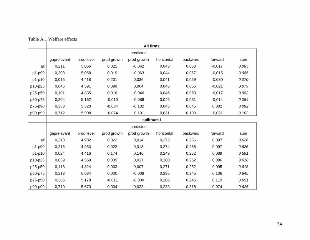
Table A.1 Welfare effects All firms

gaprelevant prod level prod growth

predicted

prod growth horizontal backward forward sum

all 0,211 5,056 0,021 -0,062 0,043 0,058 -0,017 0,085

p1-p99 0,208 5,058 0,019 -0,063 0,044 0,057 -0,015 0,085

p1-p10 0,015 4,418 0,201 0,036 0,041 0,059 -0,030 0,070

p10-p25 0,046 4,591 0,099 0,004 0,045 0,055 -0,021 0,079

p25-p50 0,101 4,835 0,016 -0,046 0,046 0,053 -0,017 0,082

p50-p75 0,204 5,162 -0,010 -0,088 0,046 0,051 -0,014 0,084

p75-p90 0,383 5,520 -0,034 -0,102 0,045 0,045 0,002 0,092

p90-p99 0,712 5,908 -0,074 -0,101 0,031 0,103 -0,031 0,102

splitnum I


predicted


all 0,218 4,932 0,022 0,014 0,273 0,256 0,097 0,626

p1-p99 0,215 4,933 0,022 0,013 0,274 0,255 0,097 0,626

p1-p10 0,024 4,416 0,174 0,146 0,249 0,252 0,089 0,591

p10-p25 0,059 4,559 0,039 0,017 0,280 0,252 0,086 0,618

p25-p50 0,113 4,824 0,003 0,007 0,271 0,252 0,095 0,618

p50-p75 0,213 5,034 0,000 -0,008 0,295 0,245 0,106 0,645

p75-p90 0,385 5,178 -0,011 -0,030 0,286 0,246 0,119 0,651

p90-p99 0,710 5,670 0,004 0,023 0,233 0,318 0,074 0,625

35

splitnum II


predicted


all 0,268 5,287 -0,068 -0,066 0,001 0,010 -0,378 -0,367

p1-p99 0,267 5,286 -0,069 -0,070 0,002 0,010 -0,378 -0,366

p1-p10 0,022 4,611 0,173 0,158 0,003 0,012 -0,393 -0,378

p10-p25 0,068 4,601 0,025 -0,063 0,003 0,011 -0,382 -0,367

p25-p50 0,142 5,071 -0,073 -0,054 0,003 0,010 -0,379 -0,366

p50-p75 0,279 5,379 -0,124 -0,114 0,003 0,010 -0,368 -0,356

p75-p90 0,487 5,911 -0,109 -0,111 0,003 0,010 -0,399 -0,387

p90-p99 0,782 6,088 -0,151 -0,079 -0,009 0,008 -0,352 -0,353

splitnum III


predicted


all 0,204 4,826 -0,109 -0,119 0,404 -0,045 -0,079 0,280

p1-p99 0,198 4,820 -0,107 -0,117 0,404 -0,046 -0,078 0,280

p1-p10 0,022 4,209 0,017 -0,025 0,393 -0,069 -0,080 0,243

p10-p25 0,054 4,348 -0,086 -0,076 0,407 -0,061 -0,081 0,266

p25-p50 0,105 4,601 -0,093 -0,083 0,402 -0,055 -0,079 0,269

p50-p75 0,197 4,978 -0,106 -0,129 0,403 -0,048 -0,078 0,277

p75-p90 0,352 5,258 -0,150 -0,174 0,408 -0,032 -0,073 0,303

p90-p99 0,658 5,569 -0,193 -0,199 0,408 0,010 -0,085 0,332

36

splitnum IV


predicted


all 0,194 5,112 0,166 -0,069 0,021 0,025 -0,091 -0,045

p1-p99 0,192 5,121 0,162 -0,068 0,020 0,030 -0,097 -0,046

p1-p10 0,008 4,375 0,332 0,077 0,059 -0,275 0,122 -0,095

p10-p25 0,029 4,645 0,281 0,064 0,038 0,027 -0,142 -0,078

p25-p50 0,075 4,926 0,194 -0,042 0,031 0,025 -0,122 -0,066

p50-p75 0,172 5,166 0,125 -0,063 0,022 0,046 -0,114 -0,046

p75-p90 0,346 5,567 0,091 -0,106 0,005 0,094 -0,128 -0,029

p90-p99 0,681 5,968 0,035 -0,121 0,013 -0,041 0,007 -0,021

splitnum V


predicted


all 0,273 5,674 -0,006 0,009 -0,012 0,034 -0,364 -0,342

p1-p99 0,267 5,659 -0,007 0,008 -0,012 0,034 -0,362 -0,341

p1-p10 0,022 4,163 -0,005 0,004 -0,013 0,032 -0,298 -0,280

p10-p25 0,057 5,047 -0,066 -0,071 -0,016 0,031 -0,296 -0,281

p25-p50 0,124 5,435 0,023 0,041 -0,012 0,021 -0,280 -0,271

p50-p75 0,254 5,873 0,019 0,017 -0,017 0,016 -0,351 -0,351

p75-p90 0,506 6,199 0,028 -0,008 -0,008 0,046 -0,417 -0,380

p90-p99 0,889 6,914 0,025 0,071 -0,004 0,093 -0,662 -0,572

37

splitnum VI


predicted


all 0,226 6,045 0,104 0,084 0,075 -0,819 1,213 0,470

p1-p99 0,227 6,045 0,104 0,084 0,075 -0,819 1,226 0,483

p1-p10 0,020 4,754 0,364 0,084 0,055 -0,962 1,551 0,644

p10-p25 0,048 5,340 0,218 0,230 0,059 -0,820 1,246 0,485

p25-p50 0,096 5,579 0,172 0,152 0,034 -0,907 1,374 0,502

p50-p75 0,216 6,337 0,027 0,035 0,099 -0,722 1,086 0,463

p75-p90 0,421 6,697 -0,005 -0,008 0,103 -0,829 1,203 0,477

p90-p99 0,734 6,915 0,057 0,032 0,084 -0,768 1,059 0,375

splitnum VII


predicted


all 0,251 5,376 -0,261 -0,270 -0,042 0,171 0,085 0,214

p1-p99 0,254 5,378 -0,260 -0,270 -0,042 0,171 0,085 0,214

p1-p10 0,021 4,333 -0,143 -0,171 0,015 0,191 0,092 0,299

p10-p25 0,064 4,924 -0,247 -0,268 -0,017 0,167 0,089 0,238

p25-p50 0,151 5,203 -0,315 -0,335 -0,035 0,164 0,093 0,222

p50-p75 0,318 5,722 -0,307 -0,303 -0,073 0,156 0,089 0,172

p75-p90 0,561 6,119 -0,185 -0,197 -0,036 0,191 0,097 0,252

p90-p99 0,899 6,214 -0,147 -0,106 -0,108 0,209 -0,018 0,083

Openness, competition, technology and FDI spillovers: Evidence from Romania

Documents

Transcript of Openness, competition, technology and FDI spillovers: Evidence from Romania