Unbelievably preliminary. Cite this and you’re cactus.

Migration, Trade and FDI in Mexico

Patricio Aroca Universidad Catolica del Norte, Antofagasta, Chile

W.F. Maloney

Office of the Chief Economist for Latin America The World Bank

April 15, 2002

“Mexico wants to export goods, not people.”

Carlos Salinas de Gortari I. Introduction

Mexican President Carlos Salinas de Gortari promoted NAFTA partly on the

grounds that it would reduce the incentives for Mexicans to migrate north. Yet what

limited evidence there is does not strongly support this claim. As Razin and Sadka

(1997) note, theoretically trade and to a lesser degree capital flows, and migration can be

complements. Markusen and Zahniser (1999), drawing on models by Feenstra and

Hanson (1995) and Markusen and Venables (1995) study the effects of NAFTA on the

convergence in the wages of unskilled workers between the two countries and they echo

the widely held view that NAFTA will do little to achieve wage convergence and hence

deter migration.

This paper attempts to measure the direct impact of foreign direct investment and

trade on migration. Ideally, we would answer the question using actual data on Mexican-

US migration, but the illicit nature of these flows and generally poor quality of the data

makes such a direct approach difficult. The paper instead asks whether these variables

have had any impact on flows within Mexico where the census data permit careful

analysis. We find that they do and that both FDI and exports are substitutes for labor

flows- they deter migration. We then generate some tentative inferences about the impact

on Mexico-US migration and find it to be of important magnitude.

In the process, we also generate the first estimates of determinants of migration

flows within Mexico. In line with recent advances in the industrialized country literature,

we generate proxies for both the level of amenities and costs of living and find their

influence statistically significant. Contrary to much of the literature, we also find very

significant and very intuitively plausible signs on labor market variables. The signs on

all these variables confirm the often postulated liquidity effect- it takes resources to

move.

1

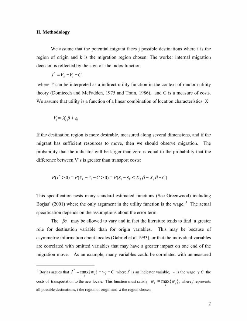
II. Methodology

We assume that the potential migrant faces j possible destinations where i is the

region of origin and k is the migration region chosen. The worker internal migration

decision is reflected by the sign of the index function

CVVI ik −−=*

where V can be interpreted as a indirect utility function in the context of random utility

theory (Domicech and McFadden, 1975 and Train, 1986), and C is a measure of costs.

We assume that utility is a function of a linear combination of location characteristics X

Vj = Xj β + εj

If the destination region is more desirable, measured along several dimensions, and if the

migrant has sufficient resources to move, then we should observe migration. The

probability that the indicator will be larger than zero is equal to the probability that the

difference between V’s is greater than transport costs:

)()0()0( * CXXPCVVPIP ikkiik −−≤−=>−−=> ββεε

This specification nests many standard estimated functions (See Greenwood) including

Borjas’ (2001) where the only argument in the utility function is the wage. 1 The actual

specification depends on the assumptions about the error term.

The βs may be allowed to vary and in fact the literature tends to find a greater

role for destination variable than for origin variables. This may be because of

asymmetric information about locales (Gabriel et.al 1993), or that the individual variables

are correlated with omitted variables that may have a greater impact on one end of the

migration move. As an example, many variables could be correlated with unmeasured

1 Borjas argues that where I* is an indicator variable, w is the wage y C the

costs of transportation to the new locale. This function must satisfy , where j represents

all possible destinations, i the region of origin and k the region chosen.

CwwI ijj−−= }{max*

}{max jjk ww =

2

wealth or liquidity that would determine whether the worker has the savings to pay the

fixed cost C of moving (See Vanderkamp 1972).

The matrix X contains the variables capturing the relative expected incomes (Y)

in the two areas(wages, unemployment, price indices), and the set of characteristics of the

region (amenities) that may also affect the migration decision. It is through Y that we

might expect the impact of FDI and trade. As the survey by Razin and Sadka (1997)

argues, migration and trade, and to a lesser degree FDI may be substitutes or

complements and hence there is no guarantee that NAFTA would necessarily, on purely

theoretical grounds, lead to lower migration.

Since we work with aggregate data, we follow Berkson’s (1944) setup as

elaborated by Ben-Akiva and Lerman (1985) and generalized in Gourieroux (2000). Here

CXXIPF oidk −−=>− ββ))0(( *1

where F is the probability function that is determined by the structure of the errors.

III. Data

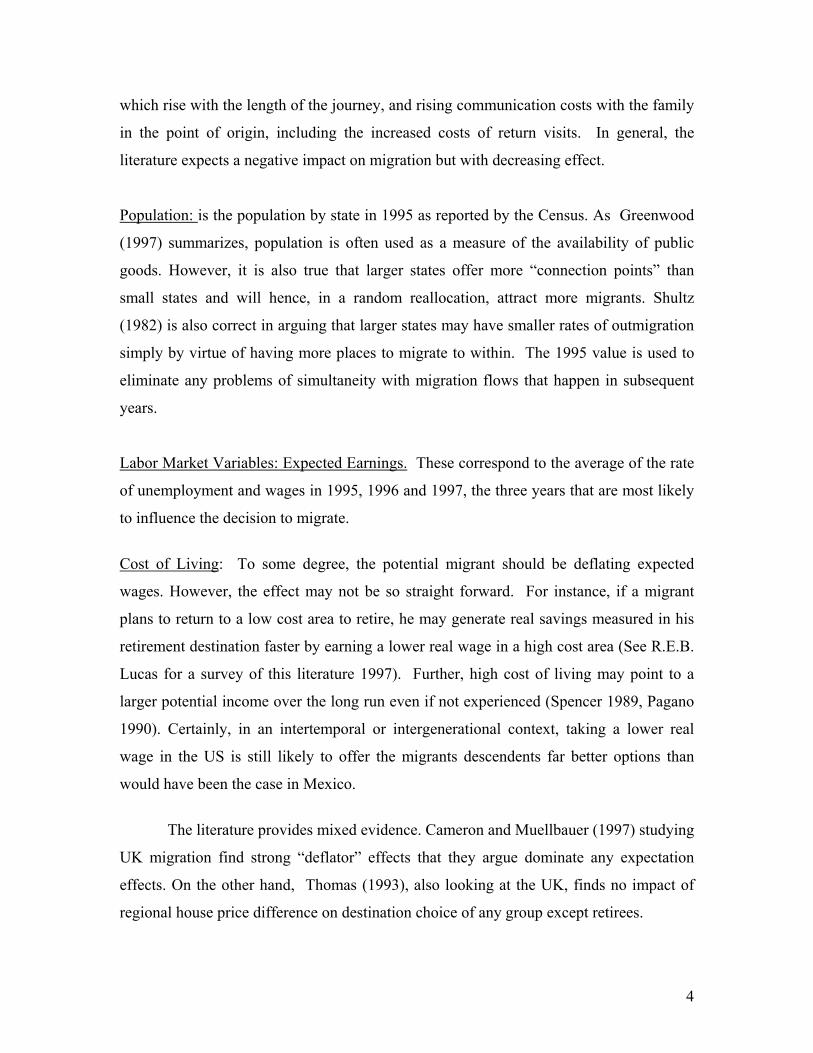
Migration data: The 2000 census tabulates the question “In which state did you reside

five years ago?” (¿En qué estado vivía usted hace 5 años?) and then this response is

compared with the present state. As with most data of this type, this has the drawback of

obscuring migrants who may have left and returned in the five year period. Graph 1

shows the rates of Net Migration by states. The variable is calculated as net flows as a

fraction of the population in the initial period.

Moving Costs: Following the literature (again, see Greenwood), we approximate the

costs of transportation as a quadratic function of distance.2 This is a proxy for the costs

of migration that consist of the moving costs themselves, the opportunity costs of moving

2 Though we assume that the indirect utility function is linear and the weight of each variable is similar in each region, this assumption can be easy relaxed to differentiate the origin (o) and destination (d) parameters.

3

which rise with the length of the journey, and rising communication costs with the family

in the point of origin, including the increased costs of return visits. In general, the

literature expects a negative impact on migration but with decreasing effect.

Population: is the population by state in 1995 as reported by the Census. As Greenwood

(1997) summarizes, population is often used as a measure of the availability of public

goods. However, it is also true that larger states offer more “connection points” than

small states and will hence, in a random reallocation, attract more migrants. Shultz

(1982) is also correct in arguing that larger states may have smaller rates of outmigration

simply by virtue of having more places to migrate to within. The 1995 value is used to

eliminate any problems of simultaneity with migration flows that happen in subsequent

years.

Labor Market Variables: Expected Earnings. These correspond to the average of the rate

of unemployment and wages in 1995, 1996 and 1997, the three years that are most likely

to influence the decision to migrate.

Cost of Living: To some degree, the potential migrant should be deflating expected

wages. However, the effect may not be so straight forward. For instance, if a migrant

plans to return to a low cost area to retire, he may generate real savings measured in his

retirement destination faster by earning a lower real wage in a high cost area (See R.E.B.

Lucas for a survey of this literature 1997). Further, high cost of living may point to a

larger potential income over the long run even if not experienced (Spencer 1989, Pagano

1990). Certainly, in an intertemporal or intergenerational context, taking a lower real

wage in the US is still likely to offer the migrants descendents far better options than

would have been the case in Mexico.

The literature provides mixed evidence. Cameron and Muellbauer (1997) studying

UK migration find strong “deflator” effects that they argue dominate any expectation

effects. On the other hand, Thomas (1993), also looking at the UK, finds no impact of

regional house price difference on destination choice of any group except retirees.

4

Two indices were constructed and the methodologies are detailed in annex I. The

first is a hedonically estimated housing price that is the analogue to those used elsewhere

in the industrial country literature. Since food is likely comprise a larger share of the

consumption basket in LDCs, we also generate the cost of a basic food basket by state.

These were included both separately and as an average measure of the cost of living.

Amenities: Price indices, however, may also simply reflect amenities available in the

new area, implying a positive relation with migration decisions. Further, as Roback

(1982) showed, they affect equilibrium wages as well and hence should be included as

part of the net utility change of moving from one region to another. To attempt to control

for this, we extract the principal component of a set of variables that include health,

education, and infrastructure services (see Annex II).

Trade and Investment Variables

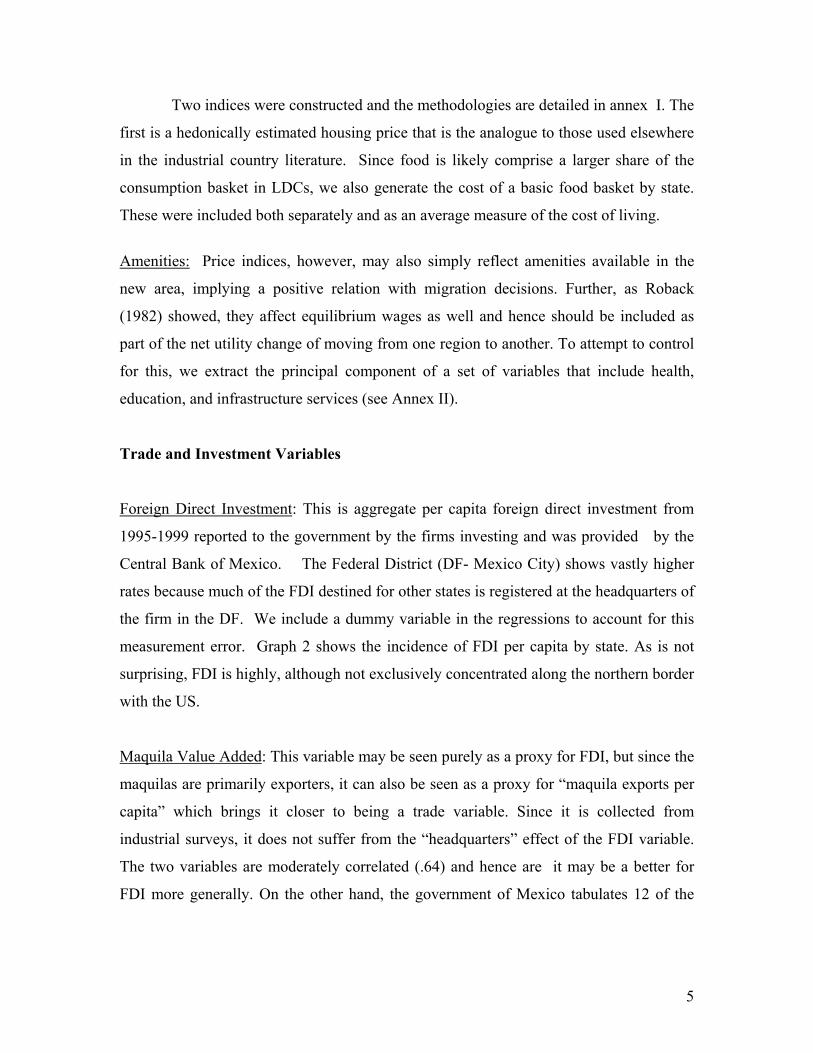
Foreign Direct Investment: This is aggregate per capita foreign direct investment from

1995-1999 reported to the government by the firms investing and was provided by the

Central Bank of Mexico. The Federal District (DF- Mexico City) shows vastly higher

rates because much of the FDI destined for other states is registered at the headquarters of

the firm in the DF. We include a dummy variable in the regressions to account for this

measurement error. Graph 2 shows the incidence of FDI per capita by state. As is not

surprising, FDI is highly, although not exclusively concentrated along the northern border

with the US.

Maquila Value Added: This variable may be seen purely as a proxy for FDI, but since the

maquilas are primarily exporters, it can also be seen as a proxy for “maquila exports per

capita” which brings it closer to being a trade variable. Since it is collected from

industrial surveys, it does not suffer from the “headquarters” effect of the FDI variable.

The two variables are moderately correlated (.64) and hence are it may be a better for

FDI more generally. On the other hand, the government of Mexico tabulates 12 of the

5

states in an “other” other category and hence we lose substantial information. We run the

regressions with the substantially reduced sample.

Exports: This variable is provided by the Ministry of Finance (Hacienda) and is alleged

to capture exports per state. However, it may be that this represents interpolations by the

government based on employment in industry as measured by the IMSS (Pending

verification).

Imports: Provided by Bancomext. This variable could have multiple and conflicting

effects. It could simply reflect the degree of integration of a state with external

economies and hence proxy as well for exports. On the other hand, if it is seen as

representing competition for import substituting firms, the short run labor market impact

could be negative and hence it could conceivably lead to more migration.

None of the variables are ideal, but they are complementary in the sense of being strong

whether the other is weak. Together, we may get some reliable picture of the impact of

trade/investment variables.

IV. Results

In preliminary regressions, we estimated a multinomial logit model for aggregate

data. Though the results were consistent with the theory, the Fry and Harris test (1998)

suggest that the data violated the Independence of Irrelevant Alternative (IIA). Therefore,

we estimate a multinomial probit and follow Gourieroux’s (2000) weighted least square

procedure.3

3 Given that the restriction on the pseudo indirect utility function that imposes the condition that all individuals in every state have an identical distribution of conditional probabilities may be strong, we follow the route suggested by Pudney (1989) that includes an alternative-specific additive constant in an otherwise invariant utility function. This constant can be interpreted as fixed effects associated with the average individual in each state and therefore measures the unobservable individual characteristics that individuals in each state use in making their decisions. As in Davies et al. (2001) estimating model problematic, most likely due to the large number of parameters and the likely correlation between origin characteristics and state fixed effects. 3 Where Davies et al tackled the problem by respecifying arbitrarily the variable associated between state, joining the states that

6

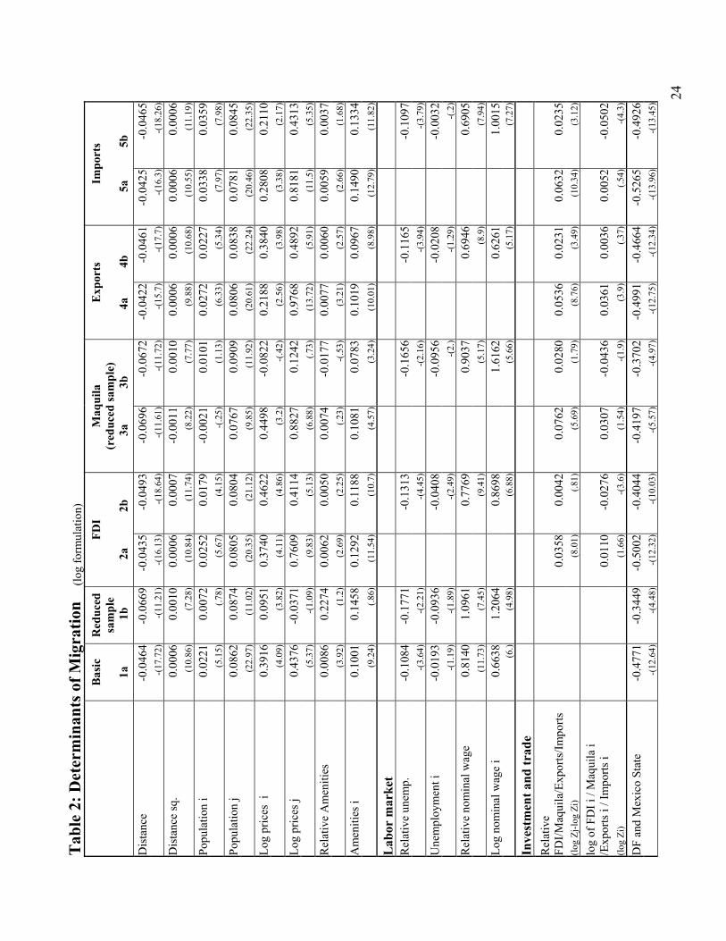
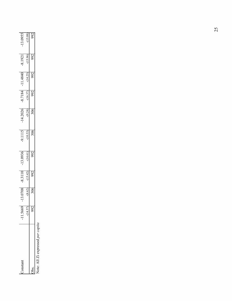
Column1 and la present the standard regression including the labor market

variables. Overall, the specifications are very satisfactory with the coefficients on the

core variables are all statistically different from zero and of predicted sign. [The distance

measure is at the low end, but firmly within the usual range of -.02 to -.2 (Greenwood,

see also Gabriel et al 1996, Fields 1982, and Schultz, 1982) and the population variables

are also consistent with usual results.

Preliminary regressions found both the origin unemployment and wage level to be

insignificant as has been found frequently in the literature (Greenwood, Lucas 1997).

However, we then attempted to isolate two countervailing effects, one a substitution

effect among regions, and the other a wealth or liquidity effect that allows the worker to

cover the fixed cost of moving. The latter effect has been found for unemployment by

Goss and Schoening (1984) and Herzog et al. (1993) for the US who find that the

probability of moving decreases with the duration of unemployment, and the literature on

the wage effect is also extensive (See Stark and Taylor 1991 for a discussion of credit

constraints). We generate relative wage (ln wj-ln wi) and relative unemployment

(Uj/Ui) variables, and then allowing free standing initial wage and unemployment

variables to capture credit constraint effects. In the complete sample, all but the free

standing unemployment term enter significantly although it is of predicted sign and

significant at the 10% level in the restricted regression. This overall strong performance

suggests that the poor results of origin labor market variables in many previous studies

arises precisely because they capture two contradictory tendencies.

The cost of living variable enters very significantly and of important magnitude in

the sector of origin. The strong positive coefficient on the destination is unexpected,

share similar unobservable characteristics, we follow a different approach. We proceed to estimate stepwise based on the initial parameters of the model, and choosing the dummy variables according to their contribution to the model.

7

although perhaps consistent with the view of cost of living being a measure of

expectations for future income growth as discussed earlier.

The amenities variable also enters with predicted signs, but again in the

relative/free standing format that suggests that amenities may be correlated with an

omitted credit constraint variable. It is not significant in the restricted sample although

the signs are as predicted.

Integration Variables

Columns 2a,3a,4a,5a drop the labor force variables and replaces them with the the

trade and investment variables in Z. In all cases, we find evidence of a strong

substitution effect: FDI and trade reduce migration. In most cases, simply entering the

initial and final terms yielded symmetrical results. However, a free standing term was

significant or borderline in half the cases suggesting again, a liquidity/wealth effect so the

results are again reported in the constrained/free standing form. All other coefficients

remain relatively unchanged with the exception of the destination price term which

appears to almost double.

Columns 2b, 3b, 4b, and 5b add the labor force variables and confirms that some,

but not all of the effect of Z works through the labor market at the same time. The

substitution effect diminishes by at least a factor of 2 in more cases and in the case of FDI

becomes insignificant. The free standing terms also show propensity to flip sign

suggesting that initial FDI was capturing the initial wealth/liquidity now capture by initial

wages and unemployment and that, minus this, local Z has a more powerful deterent

effect than destination an attractive effect. The fact that all Z retain an effect outside of

the contemporaneous labor market variables may reflect that there is an independent

disincentive effect to migrate, perhaps through expectations of future growth.

8

In short, Salinas was correct to suppose that NAFTA, through various channels,

would lead to reduced migration, at least within Mexico. The next section attempts to

quantify how large these effects might be in the context of US/Mexican migration.

V. Simulations

With the estimate above, we attempt to make some inferences about the impact of

foreign investment or Trade on migration to the US. The key assumption is that we can

treat the US as a “33rd Mexican State.” It is probably not too far out of sample to make

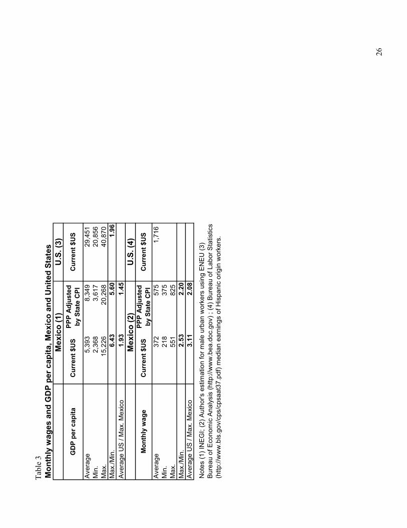
predictions. As table 3 shows, ratio of the per capita income of Mexico’s richest state,

the D.F. relative to its poorest is about 6.4 in nominal or 5.6 in real terms while the ratio

of the average for the US relative to the D.F. is only about 1.9 or 2.3 PPP adjusted. That

is, in terms of development the US is closer to Mexico City than Mexico City is to

Chiapas. Nor are wage differentials radically different. The ratio of the Hispanic real

wage in the US to the mean wage of the DF adjusted for PPP is roughly the same as the

ratio of the real DF wage to that in Chiapas.

There may be some concern about the importance of the border representing

fundamentally different “transport costs.” In fact, the evidence is strong that this is more

a difference in magnitude than kind. Donato, Durand and Massey (1992) argue that “our

data from Mexico reveal a fairly high probability of apprehension by INS combined with

a near-certain probability of ultimately entering the United States.”(p 152) and that

“every migrant who attempted a border crossing, whether apprehended or not, eventually

gained entry” p 155 italics theirs. This suggests that border control serves more as a tariff

than a quota.

The costs of movement are substantially different, but perhaps not so much as we

might think at first look. The present (2002) cost of a second class bus from Quintana

Roo to Coahuila, one of longer trips in our sample, was roughly $US100 compared to

9

very little between Mexico State and DF.4 Anecdotal evidence about the cost of direct

transport across the border in the 1980s was $150 (244 $US 2002 CHECK; Conover

1987 cited in Hanson and Spilimbergo 1999), again, not so far out of sample.5 That is

the Mex/US cost is roughly 2.5 time the ratio Max/Min within Mexico- not too far out of

sample. The cost of a Coyote or smuggler/guide appears to have held steady in real terms

since the 1960s at around $350 ( $2075 $US2002; Donato, Durand and Massey 1992) 6

although Crane et al (1990 cited in Hanson and Spilimbergo 1999) suggest that in 1993

only 8.3 percent of those apprehended by the INS had employed one. Clearly, the

premium for risk involved in crossing the border and for the multiple trips will widen the

gap substantially. Even if these gaps are wide, eq (1) suggests that the coefficients on the

components of the indirect utility functions should be separable from those of the cost of

travel. That is, the travel cost elasticity may not be suitably estimated for forecasting the

impact of a change in Mex/US travel costs, but the response to wages, FDI or exports

should not be affected.

Under these assumptions, we can think of the estimates above in two ways. First,

as corresponding to those of the aggregate average Mexican state vis a vis any other state

including the US. The implicit elasticities therefore capture the reduction in push to the

US and the increased attractiveness from the US of and increase in trade or investment.

Alternatively, and with the potential for greater richness, we assume that total

emigration from any state is the sum of migration to other states plus the US:

32

1i ij

jiUSM m m

=

= +∑ for all i = 1,..., 32

32

1

*i i ijj

iUSM Pop p m=

= +∑

4 White Star Bus line 5 Inflated from 1985 figure with CPI. 6 This showed little change with the Immigration Reform and Control Act of 1986 suggesting that it is a fairly robust number. Figure was reached by inflating the 1960 figure by the CPI. Coyotes only get paid for successful crossings.

10

and that further total emigration is fixed: 32

1i

iM M

=

=∑ . This implies that we are only

concerned about the redistribution of emigrants between the Mexican states and the US in

response to a change in the X variables. This is consistent with models which postulate

a two step decision on the part of migrants- first to migrate, and then which destination to

choose. It is also only problematic to the degree that we believe that the impact on total

flows are not second order and/or that they are radically different in distribution among

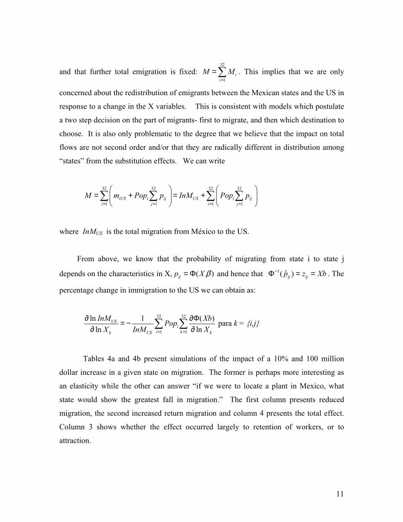
“states” from the substitution effects. We can write

32 32 32 32

1 1 1iUS i ij US i ij

i j i 1jM m Pop p InM Pop p

= = =

= + = +

∑ ∑ ∑ ∑

=

where InMUS is the total migration from México to the US.

From above, we know that the probability of migrating from state i to state j

depends on the characteristics in X, ( )ijp X β= Φ and hence that 1 ˆ( )ij ijp z X− = bΦ = . The

percentage change in immigration to the US we can obtain as:

32 32

1 1

ln 1ln ln

USi

i kk US

InM ( )

k

XbPopX InM X= =

∂ ∂Φ= −∂ ∂∑ ∑ para k = {i,j}

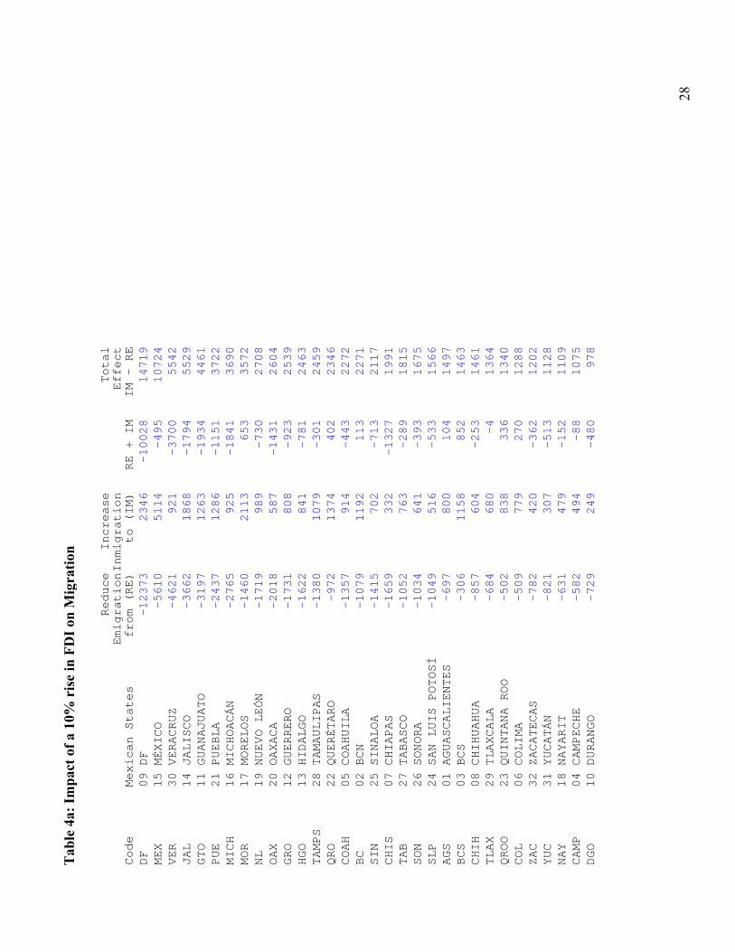
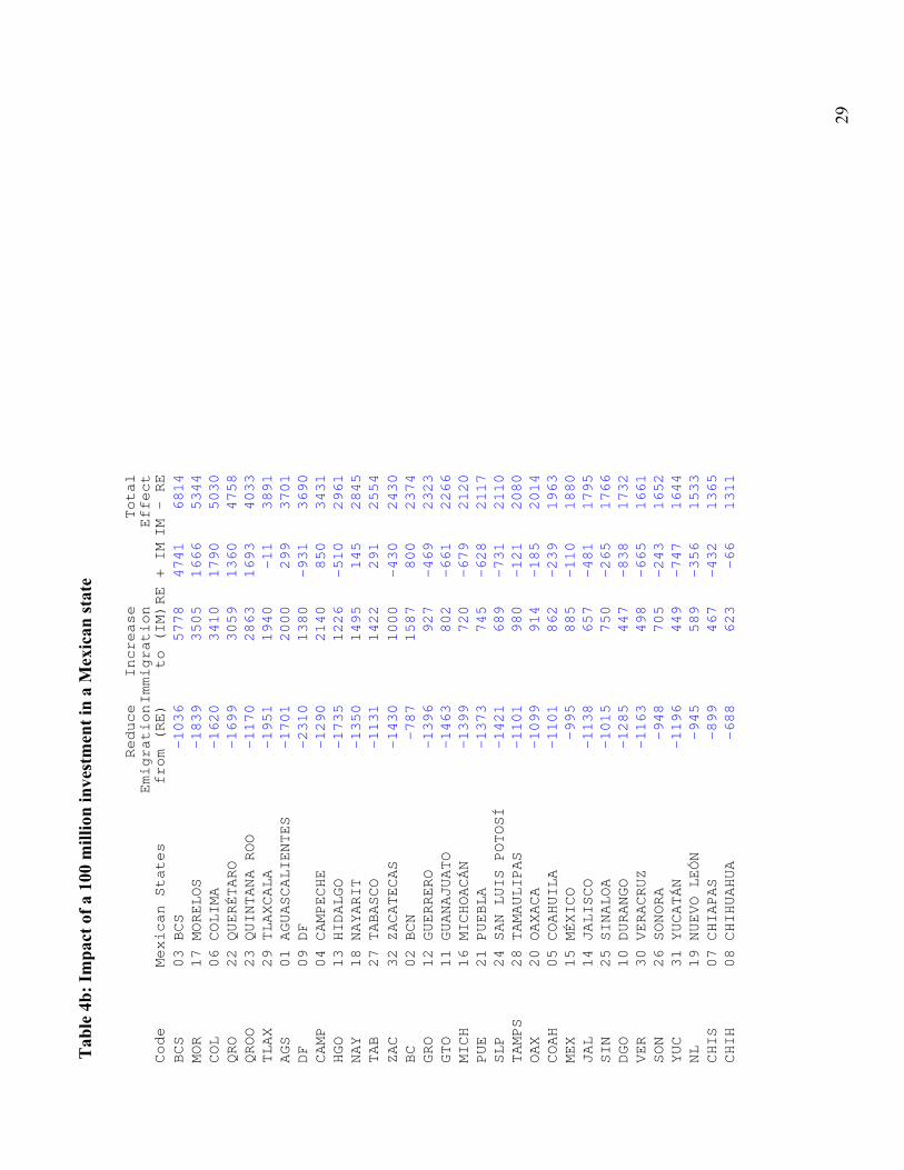
Tables 4a and 4b present simulations of the impact of a 10% and 100 million

dollar increase in a given state on migration. The former is perhaps more interesting as

an elasticity while the other can answer “if we were to locate a plant in Mexico, what

state would show the greatest fall in migration.” The first column presents reduced

migration, the second increased return migration and column 4 presents the total effect.

Column 3 shows whether the effect occurred largely to retention of workers, or to

attraction.

11

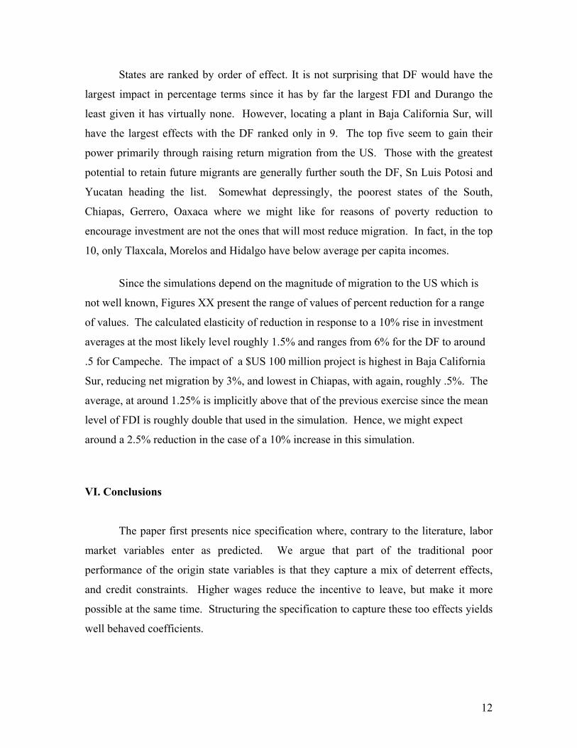
States are ranked by order of effect. It is not surprising that DF would have the

largest impact in percentage terms since it has by far the largest FDI and Durango the

least given it has virtually none. However, locating a plant in Baja California Sur, will

have the largest effects with the DF ranked only in 9. The top five seem to gain their

power primarily through raising return migration from the US. Those with the greatest

potential to retain future migrants are generally further south the DF, Sn Luis Potosi and

Yucatan heading the list. Somewhat depressingly, the poorest states of the South,

Chiapas, Gerrero, Oaxaca where we might like for reasons of poverty reduction to

encourage investment are not the ones that will most reduce migration. In fact, in the top

10, only Tlaxcala, Morelos and Hidalgo have below average per capita incomes.

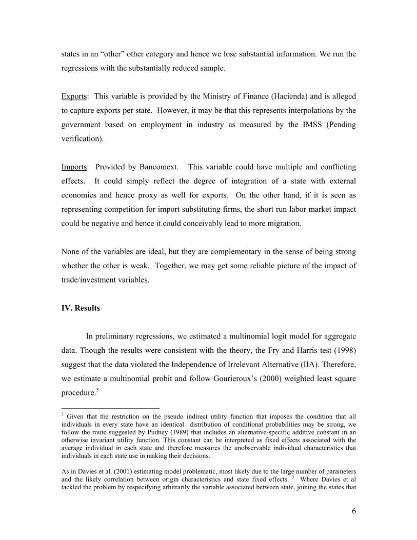
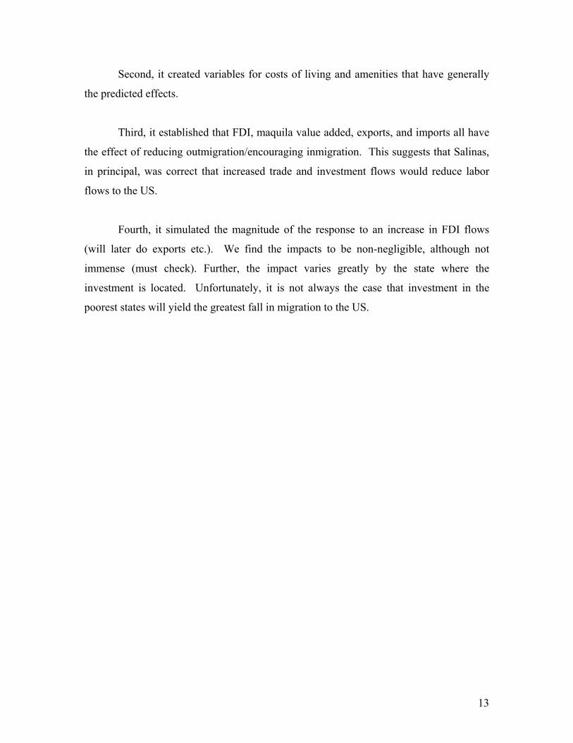
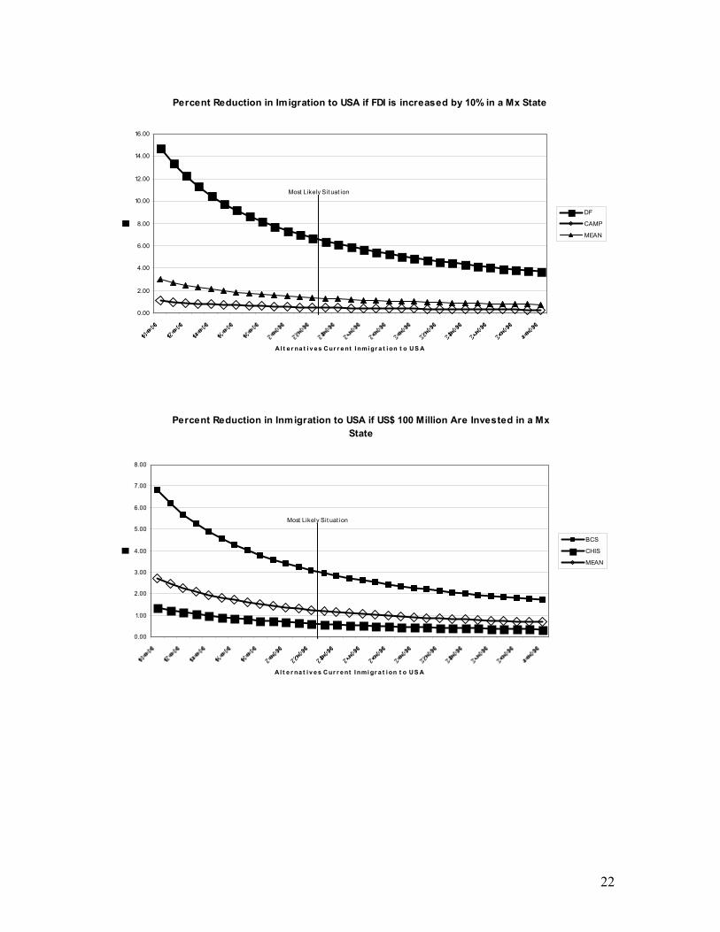
Since the simulations depend on the magnitude of migration to the US which is

not well known, Figures XX present the range of values of percent reduction for a range

of values. The calculated elasticity of reduction in response to a 10% rise in investment

averages at the most likely level roughly 1.5% and ranges from 6% for the DF to around

.5 for Campeche. The impact of a $US 100 million project is highest in Baja California

Sur, reducing net migration by 3%, and lowest in Chiapas, with again, roughly .5%. The

average, at around 1.25% is implicitly above that of the previous exercise since the mean

level of FDI is roughly double that used in the simulation. Hence, we might expect

around a 2.5% reduction in the case of a 10% increase in this simulation.

VI. Conclusions

The paper first presents nice specification where, contrary to the literature, labor

market variables enter as predicted. We argue that part of the traditional poor

performance of the origin state variables is that they capture a mix of deterrent effects,

and credit constraints. Higher wages reduce the incentive to leave, but make it more

possible at the same time. Structuring the specification to capture these too effects yields

well behaved coefficients.

12

Second, it created variables for costs of living and amenities that have generally

the predicted effects.

Third, it established that FDI, maquila value added, exports, and imports all have

the effect of reducing outmigration/encouraging inmigration. This suggests that Salinas,

in principal, was correct that increased trade and investment flows would reduce labor

flows to the US.

Fourth, it simulated the magnitude of the response to an increase in FDI flows

(will later do exports etc.). We find the impacts to be non-negligible, although not

immense (must check). Further, the impact varies greatly by the state where the

investment is located. Unfortunately, it is not always the case that investment in the

poorest states will yield the greatest fall in migration to the US.

13

REFERENCES

Ben-Akiva, M. and S.R. Lerman (1985). Discrete Choice Analysis. Theory and Application to Travel Demand. MIT Press, Cambridge, MA, USA Beyer, H., P. Rojas and R. Vergara (1999). Trade Liberalization and Wage Inequality. Journal of Development Economics, 59: 103-123. Borjas, George (2001). Does Immigration Grease the Wheels of the Labor Market?. Brooking Panel on Economics Activity, March 29-30. Available on http://www.brook.edu/es/events/bpea/200103/0101_papers.htm Borjas, George (1994 “The Economics of Immigration,” Journal of Economic Literature, 32:1667-717 Cameron, Gavin, and John Muellbauer (1998) “The Housing Market and Regional Commuting and Migration Choices.” Centere for Economic Policy Research, Discussion Paper no. 1945. Conover, Ted (1987) Coyotes: A Journey through the Secret World of America’s Illegal Aliens. New York: Vintage. Crane, Keith, W., Beth J. Asch, Joanna Z Heilbrunn, and Danielle C. Cullinane, (1990) “The Effect of Employer Sanctions on the Flow of Undocumented Immigrants to the United States.” Urban Institute Report No. 90-8, Washington, DC, 1990. Davies, P.S., M.J. Greenwood and H. Li (2001). A Conditional Logit Approach to U.S. State-To-State Migration. Journal of Regional Science, Vol. 41, No. 2, pp.337-360. Domecich, T.A., and D. McFadden (1975). Urban Travel Demand. A Behavioral Analysis. North Holland Publishing Co., NY, USA. Donato, Katharine M. Jorge Druand and Douglas S. Massey (1992), “Stemming the Tide? Assessing the Deterrent Effects of the Immigration Reform and Control Act” Demography, 29:139-157. Faini, R., J-M. Grether and J. De Melo (1999). Globalisation, and migratory pressures from developing countries: a simulation analysis. Published in Migration. The Controversies and the Evidence, Ed. By R. Faini, J. De Melo and K.F. Zimmermann, Cambridge University Press, Cambridge, UK. Feenstra, R.C. and G.H. Hanson (1995). Foreign Direct Investment and Realtive Wages: Evidence from Mexico’s Maquiladoras. NBER wp 5122, Cambridge, MA, USA.

14

Field, G. (1982). Place-to-Place Migration in Colombia. Economic Development and Cultural Change, 31, pp. 538-558. Fry, T.R.L. and M.N. Harris (1998). Testing for Independence of Irrelevant Alternatives. Some Empirical Results. Sociological Methods & Research. Vol 26 No 3, pp. 401-423. Gabriel, S.A., J. Shack-Marquez and W.L. Wascher (1996). Does Migration Arbitrage Regional Labor Market Differentials? Regional Science and Urban Economics, 23, pp. 211-233. Goss, E. P and N.C. Schoening (1984), “ Search time, Unemployment and the Migration Decision,” Journal of Human Resources, 19:570-579 Gourieroux, Christian (2000). Econometrics of Qualitative Dependent Variables. Cambridge University Press, Cambridge, UK. Greenwood, M. J. (1997). “Internal Migration in Developed Countries”. In Handbook of Families and Population Economics. Rosenzweig and Stark (Eds.). North-Holland, Amsterdam. Hanson, Gordon and Antonio Spillembergo (1999) “Illegal Immigration, Border Enforcemtn, and Relative Wages: Evidence from Apprehensions at the U.S.-Mexico Border” American Economic Review 89:1337-1357 Herzog, H.W. Jr., A.M. Schlottmann and T.P Boehm (1993), “Migration as Spatial JobSearch: A Survey of Empirical Findinggs”, Regional Studies 27:605-620. Leonard, J.S. and R. McCulloch (1991). Foreign-Owned Businesses in the United State. Published in Immigration, Trade and the Labor Market, Ed. By J.M. Abowd and R.B. Freeman, NBER Project Report, The University of Chicago Press, Chicago, USA. Lucas, R.E.B. (1997) “Internal Migration in Developing Countries,” In Handbook of Families and Population Economics. Rosenzweig and Stark (Eds.). North-Holland, Amsterdam. Markusen, J.R. and S. Zahniser (1999). Liberalisation and incentives for labour migration: theory with applications to NAFTA. Published in Migration. The Controversies and the Evidence, Ed. By R. Faini, J. De Melo and K.F. Zimmermann, Cambridge University Press, Cambridge, UK. Markusen, J.R. and A.J. Venables (1997) “The Role of the Multinational Firm in the Wage-Gap Debate,” Review of International Economics,5:435-51 Pagano, M. (1990 “Discussion of Muellbauer and Murpher (1990) “Is the Balance of Payments Sustainable? Economic Policy 5:387-390. Cited in Cameron and Muellbauer (1998)

15

Pudney, S. (1989). Modeling Individual Choice. The Econometrics of Corners, Kinks and Holes. Basil Blackwell, Oxford, Uk. Roback, Jennifer (1982), “Wages, Rents and the Quality of Life” Journal of Political Economy 6:1257-1278. Sjaastad, Larry A. (1962) “The Costs and Returns of Human Migration.” Journal of Political Economy 70:80-93. Shultz, T.P. (1982). Lifetime Migration Within Educational Strata in Venezuela: Estimates of a Logistic Model. Economic Development and Cultural Change, 31, pp. 559-593. Spencer, P.D. (1989), “Comments on Bover et al” (1989), Oxford Bulletin of Economics and Statistics, 51: 153-157. Cited in Cameron and Muellbauer (1998). Stark, Oded, and J. Edward Taylor(1991) “Migration Incentives, Migration Types: The Role of Relative Deprivation, The Economic Journal, 101:1163-1178. Thomas, Alun (1993) “The Influence of Wages and House Prices on British Interregional Migration Decisions,” Applied Economics 25:1261-1268. Train, Kenneth (1986). Qualitative Choice Analysis. Theory, Econometrics, and an Application to the Automobile Demand. The MIT Press, Cambridge, MA, USA. Vanderkamp, J. (1971) “Migration Flows, their Determinants and the Effects of Return Migration,” Journal of Political Economy, 79:1012-1031.

16

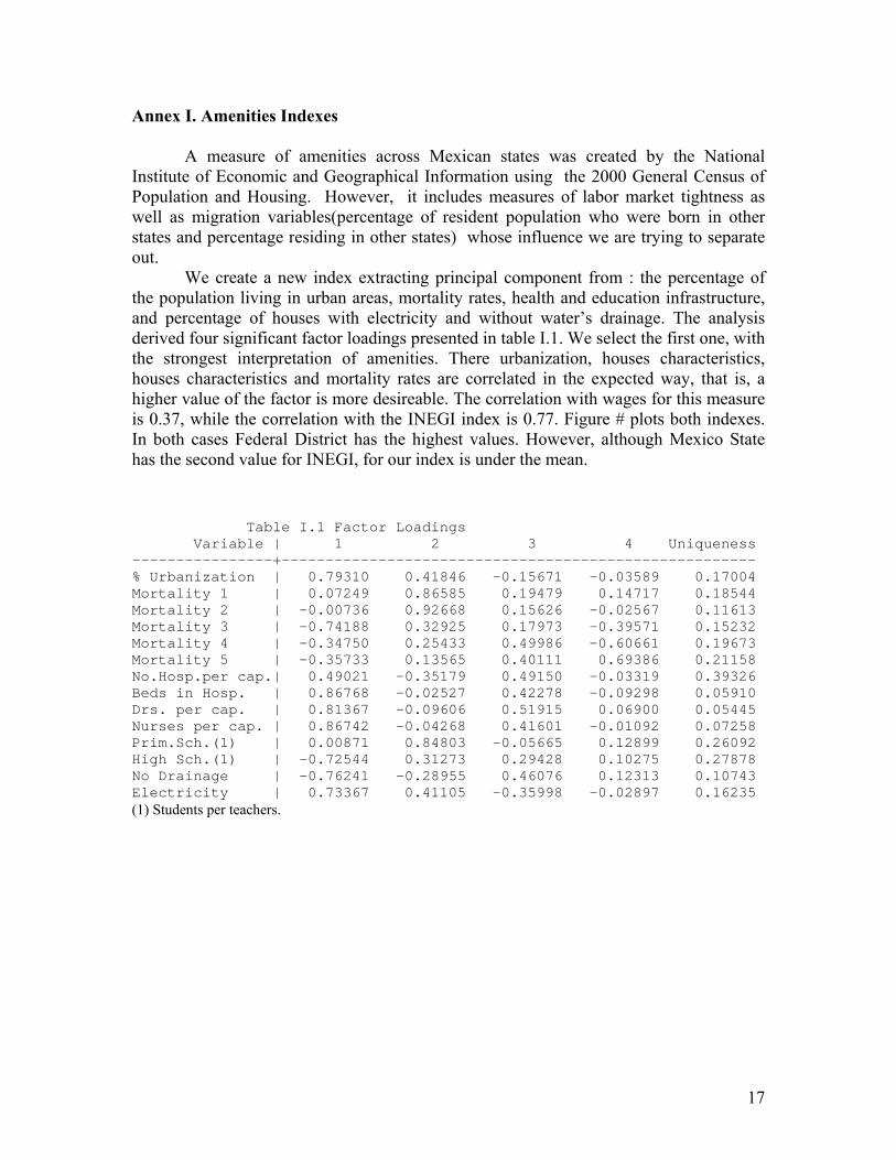
Annex I. Amenities Indexes

A measure of amenities across Mexican states was created by the National Institute of Economic and Geographical Information using the 2000 General Census of Population and Housing. However, it includes measures of labor market tightness as well as migration variables(percentage of resident population who were born in other states and percentage residing in other states) whose influence we are trying to separate out. We create a new index extracting principal component from : the percentage of the population living in urban areas, mortality rates, health and education infrastructure, and percentage of houses with electricity and without water’s drainage. The analysis derived four significant factor loadings presented in table I.1. We select the first one, with the strongest interpretation of amenities. There urbanization, houses characteristics, houses characteristics and mortality rates are correlated in the expected way, that is, a higher value of the factor is more desireable. The correlation with wages for this measure is 0.37, while the correlation with the INEGI index is 0.77. Figure # plots both indexes. In both cases Federal District has the highest values. However, although Mexico State has the second value for INEGI, for our index is under the mean.

Table I.1 Factor LoadingsVariable | 1 2 3 4 Uniqueness

----------------+------------------------------------------------------% Urbanization | 0.79310 0.41846 -0.15671 -0.03589 0.17004Mortality 1 | 0.07249 0.86585 0.19479 0.14717 0.18544Mortality 2 | -0.00736 0.92668 0.15626 -0.02567 0.11613Mortality 3 | -0.74188 0.32925 0.17973 -0.39571 0.15232Mortality 4 | -0.34750 0.25433 0.49986 -0.60661 0.19673Mortality 5 | -0.35733 0.13565 0.40111 0.69386 0.21158No.Hosp.per cap.| 0.49021 -0.35179 0.49150 -0.03319 0.39326Beds in Hosp. | 0.86768 -0.02527 0.42278 -0.09298 0.05910Drs. per cap. | 0.81367 -0.09606 0.51915 0.06900 0.05445Nurses per cap. | 0.86742 -0.04268 0.41601 -0.01092 0.07258Prim.Sch.(1) | 0.00871 0.84803 -0.05665 0.12899 0.26092High Sch.(1) | -0.72544 0.31273 0.29428 0.10275 0.27878No Drainage | -0.76241 -0.28955 0.46076 0.12313 0.10743Electricity | 0.73367 0.41105 -0.35998 -0.02897 0.16235(1) Students per teachers.

17

Cre

ated

Fac

tor

Amenities measuresINEGI Welfare Index

1 2 3 4 5 6 7

0

2

4

6

18

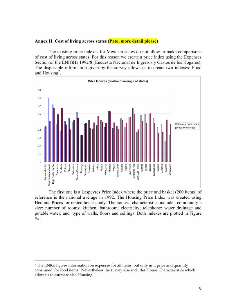
Annex II. Cost of living across states (Pato, more detail please) The existing price indexes for Mexican states do not allow to make comparisons of cost of living across states. For this reason we create a price index using the Expenses Section of the ENIGHs 1992/8 (Encuesta Nacional de Ingresos y Gastos de los Hogares). The disposable information given by the survey allows us to create two indexes: Food

The f

and Housing7.

one is a Laspeyres Price Index where the price and basket (200 items) of referen

irst

Price Indexes (relative to average of states)

0

0.2

0.4

0.6

0.8

1

1.2

1.4

1.6

1.8

Agua

scal

ient

esBa

ja C

alifo

rnia

Nor

teBa

ja C

alifo

rnia

Sur

Cam

pech

eC

oahu

ilaC

olim

a C

hiap

asC

hihu

ahua

Dis

trito

Fed

eral

Dur

ango

Gua

naju

ato

Gue

rrero

Hid

algo

Jalis

coM

exic

oM

icho

acan

Mor

elos

Nay

arit

Nue

vo L

eon

Oax

aca

Pueb

laQ

uere

tario

Qui

ntan

a R

ooSa

n Lu

is P

otos

iSi

nalo

aSo

nora

Taba

sco

Tam

aulip

asTl

axca

laVe

racr

uzYu

cata

nZa

cate

cas

Housing Price IndexFood Price Index

ce is the national average in 1992. The Housing Price Index was created using Hedonic Prices for rented houses only. The houses’ characteristics include : community’s size; number of rooms; kitchen; bathroom; electricity; telephone; water drainage and potable water; and type of walls, floors and ceilings. Both indexes are plotted in Figure ##.

7 The ENIGH gives information on expenses for all items, but only unit price and quantity consumed for food items. Nevertheless the survey also includes House Characteristics which allow us to estimate also Housing.

19

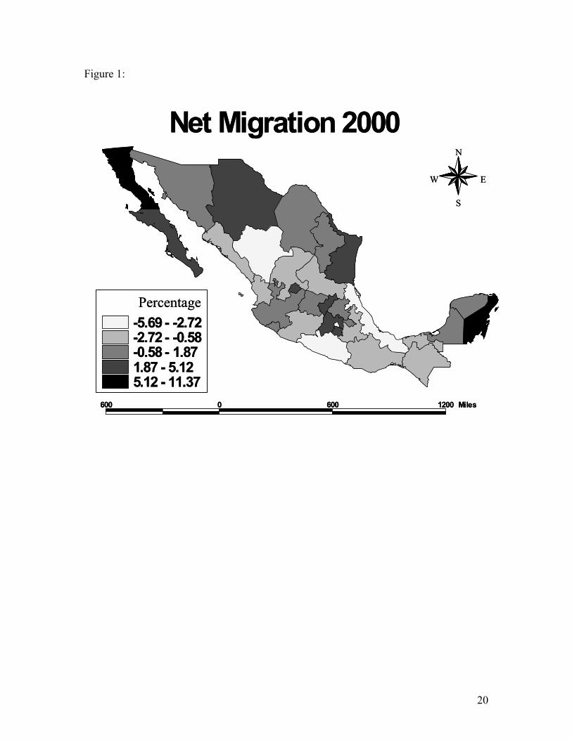
Figure 1:

-5.69 - -2.72-2.72 - -0.58-0.58 - 1.871.87 - 5.125.12 - 11.37

600 0 600 1200 Miles

N

EW

S

Net Migration 2000

Percentage-5.69 - -2.72-2.72 - -0.58-0.58 - 1.871.87 - 5.125.12 - 11.37

600 0 600 1200 Miles

N

EW

S

Net Migration 2000

Percentage

20

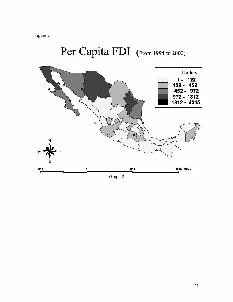
Figure 2

Graph 2

1 - 122122 - 452452 - 972972 - 18121812 - 4315

600 0 600 1200 Miles

N

EW

S

Per Capita FDI (From 1994 to 2000)

Millions of Dollars1 - 122

122 - 452452 - 972972 - 18121812 - 4315

600 0 600 1200 Miles

N

EW

S

1 - 122122 - 452452 - 972972 - 18121812 - 4315

600 0 600 1200 Miles

N

EW

S

Per Capita FDI (From 1994 to 2000)

Millions of Dollars

21

Percent Reduction in Imigration to USA if FDI is increased by 10% in a Mx State

0.00

2.00

4.00

6.00

8.00

10.00

12.00

14.00

16.00

Al t e r na t i v e s Cur r e nt I nmi gr a t i on t o US A

DF

CAMP

MEAN

Most Likely Sit uat ion

Percent Reduction in Inmigration to USA if US$ 100 Million Are Invested in a Mx State

0.00

1.00

2.00

3.00

4.00

5.00

6.00

7.00

8.00

Al t e r na t i v e s Cur r e nt I nmi gr a t i on t o US A

BCS

CHIS

MEAN

Most Likely Sit uat ion

22

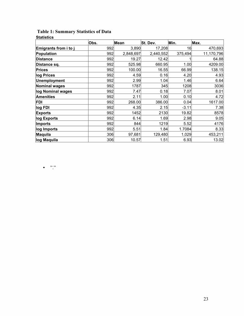
Table 1: Summary Statistics of Data Statistics Obs. Mean St. Dev. Min. Max. Emigrants from i to j 992 3,890 17,208 16 470,693 Population 992 2,848,697 2,440,552 375,494 11,170,796 Distance 992 19.27 12.42 1 64.88 Distance sq. 992 525.98 660.95 1.00 4209.00 Prices 992 100.00 16.55 66.99 138.15 log Prices 992 4.59 0.16 4.20 4.93 Unemployment 992 2.99 1.04 1.46 6.64 Nominal wages 992 1787 345 1208 3036 log Nominal wages 992 7.47 0.18 7.07 8.01 Amenities 992 2.11 1.00 0.10 4.72 FDI 992 268.00 386.00 0.04 1617.00 log FDI 992 4.35 2.15 -3.11 7.38 Exports 992 1452 2130 19.82 8578 log Exports 992 6.14 1.69 2.98 9.05 Imports 992 844 1219 5.52 4176 log Imports 992 5.51 1.84 1.7084 8.33 Maquila 306 97,681 129,480 1,029 453,211 log Maquila 306 10.57 1.51 6.93 13.02

• ”.”

23

Tab

le 2

: Det

erm

inan

ts o

f Mig

ratio

n (lo

g fo

rmul

atio

n)

Bas

ic

1a

Red

uced

sa

mpl

e 1

b

FDI

2a

2b

Maq

uila

(red

uced

sam

ple)

3a

3b

Exp

orts

4a

4b

Impo

rts

5a

5

b

Dis

tanc

e

-0

.046

4-0

.066

9-0

.043

5-0

.049

3 -0

.069

6-0

.067

2-0

.042

2-0

.046

1-0

.042

5-0

.046

5

-(17

.72)

-(

11.2

1)-(

16.1

3)-(

18.6

4)-(

11.6

1)-(

11.7

2)-(

15.7

)-(

17.7

)-(

16.3

)-(

18.2

6)D

ista

nce

sq.

0.

0006

0.00

100.

0006

0.00

07-0

.001

10.

0010

0.00

060.

0006

0.00

060.

0006

(10.

86)

(7.2

8)(1

0.84

)(1

1.74

)(8

.22)

(7.7

7)(9

.88)

(10.

68)

(10.

55)

(11.

19)

Popu

latio

n i

0.

0221

0.00

720.

0252

0.01

79-0

.002

10.

0101

0.02

720.

0227

0.03

380.

0359

(5

.15)

(.7

8)(5

.67)

(4.1

5)-(

.25)

(1.1

3)(6

.33)

(5.3

4)(7

.97)

(7.9

8)Po

pula

tion

j

0.08

620.

0874

0.08

050.

0804

0.07

670.

0909

0.08

060.

0838

0.07

810.

0845

(22.

97)

(11.

02)

(20.

35)

(21.

12)

(9.8

5)(1

1.92

)(2

0.61

)(2

2.24

)(2

0.46

)(2

2.35

)Lo

g pr

ices

i

0.

3916

0.09

510.

3740

0.46

220.

4498

-0.0

822

0.21

880.

3840

0.28

080.

2110

(4

.09)

(3

.82)

(4.1

1)(4

.86)

(3.2

)-(

.42)

(2.5

6)(3

.98)

(3.3

8)(2

.17)

Log

pric

es j

0.43

76

-0.0

371

0.76

090.

4114

0.

8827

0.12

42

0.97

68

0.48

920.

8181

0.

4313

(5

.37)

-(1.

09)

(9.8

3)(5

.13)

(6.8

8)(.7

3)(1

3.72

)(5

.91)

(11.

5)(5

.35)

Rel

ativ

e A

men

ities

0.00

860.

2274

0.00

620.

0050

0.00

74-0

.017

70.

0077

0.00

600.

0059

0.00

37

(3.9

2)

(1.2

)(2

.69)

(2.2

5)(.2

3)-(

.53)

(3.2

1)(2

.57)

(2.6

6)(1

.68)

Am

eniti

es i

0.10

010.

1458

0.12

920.

1188

0.10

810.

0783

0.10

190.

0967

0.14

900.

1334

(9

.24)

(.8

6)

(11.

54)

(10.

7)

(4.5

7)(3

.24)

(1

0.01

) (8

.98)

(12.

79)

(11.

82)

Lab

or m

arke

t

Rel

ativ

e un

emp.

-0

.108

4 -0

.177

1

-0.1

313

-0

.165

6

-0.1

165

-0

.109

7

-(3.

64)

-(2.

21)

-(

4.45

)

-(2.

16)

-(

3.94

)

-(3.

79)

Une

mpl

oym

ent i

-0

.019

3 -0

.093

6

-0.0

408

-0

.095

6

-0.0

208

-0

.003

2

-(1.

19)

-(1.

89)

-(

2.49

)

-(2.

)

-(1.

29)

-(

.2)

Rel

ativ

e no

min

al w

age

0.81

40

1.09

61

0.77

69

0.90

37

0.69

46

0.69

05

(1

1.73

) (7

.45)

(9

.41)

(5

.17)

(8

.9)

(7

.94)

Lo

g no

min

al w

age

i 0.

6638

1.

2064

0.

8698

1.

6162

0.

6261

1.

0015

(6.)

(4.9

8)

(6.8

8)

(5.6

6)

(5.1

7)

(7.2

7)

Inve

stm

ent a

nd tr

ade

Rel

ativ

e

FDI/M

aqui

la/E

xpor

ts/Im

ports

0.

0358

0.00

42

0.07

620.

0280

0.

0536

0.

0231

0.06

32

0.02

35

(log

Zj-lo

g Zi

)

(8

.01)

(.81)

(5

.69)

(1.7

9)

(8.7

6)

(3.4

9)(1

0.34

) (3

.12)

log

of F

DI i

/ M

aqui

la i

/Exp

orts

i / I

mpo

rts i

0.01

10-0

.027

6 0.

0307

-0.0

436

0.03

61

0.00

360.

0052

-0

.050

2 (lo

g Zi

)

(1

.66)

-(3.

6)

(1.5

4)-(

1.9)

(3

.9)

(.37)

(.54)

-(

4.3)

DF

and

Mex

ico

Stat

e -0

.477

1 -0

.344

9 -0

.500

2-0

.404

4

-0

.419

7-0

.370

2-0

.499

1-0

.466

4-0

.526

5-0

.492

6

-(12

.64)

-(

4.48

)-(

12.3

2)-(

10.0

3)-(

5.57

)-(

4.97

)-(

12.7

5)-(

12.3

4)-(

13.9

6)-(

13.4

5)

24

Con

stan

t

-11.

5669

-13.

0708

-8.3

110

-13.

0936

-9.1

115

-14.

2026

-8.7

184

-11.

4840

-8.1

921

-13.

0955

-(14

.57)

-(8.

62)

-(15

.42)

-(14

.61)

-(10

.53)

-(9.

24)

-(16

.37)

-(14

.25)

-(15

.96)

-(15

.08)

Obs

.

992

306

992

992

306

306

992

992

992

992

Not

e: A

ll Zi

exp

ress

ed p

er c

apita

25

Tabl

e 3

Mon

thly

wag

es a

nd G

DP

per c

apita

, Mex

ico

and

Uni

ted

Stat

esU

.S. (

3)

Aver

age

5,39

3

8,

349

29,4

51

M

in.

2,36

8

3,

617

20,8

56

M

ax.

15,2

26

20,2

68

40,8

70

M

ax./M

in.

6.43

5.60

1.96

Aver

age

US

/ Max

. Mex

ico

1.93

1.45

U.S

. (4)

Aver

age

372

57

5

1,71

6

Min

.21

8

375

M

ax.

551

82

5

Max

./Min

.2.

532.

20Av

erag

e U

S / M

ax. M

exic

o3.

112.

08

Not

es (1

) IN

EGI;

(2) A

utho

r's e

stim

atio

n fo

r mal

e ur

ban

wor

kers

usi

ng E

NEU

(3)

Bure

au o

f Eco

nom

ic A

naly

sis

(http

://w

ww

.bea

.doc

.gov

) ; (4

) Bur

eau

of L

abor

Sta

tistic

s (h

ttp://

ww

w.b

ls.g

ov/c

ps/c

psaa

t37.

pdf)

med

ian

earn

ings

of H

ispa

nic

orig

in w

orke

rs.

Mon

thly

wag

e

GD

P pe

r cap

itaC

urre

nt $

US

PPP

Adju

sted

by

Sta

te C

PI

Cur

rent

$U

SPP

P Ad

just

ed

by S

tate

CPI

C

urre

nt $

US

Mex

ico

(2)

Mex

ico

(1)

Cur

rent

$U

S

26

27

Tab

le 4

a: Im

pact

of a

10%

ris

e in

FD

I on

Mig

ratio

n

Code

MexicanStates

Reduce

Emigration

from(RE)

Increase

Inmigration

to(IM)

RE+IM

Total

Effect

IM-RE

DF

09DF

-12373

2346

-10028

14719

MEX

15MÉXICO

-5610

5114

-495

10724

VER

30VERACRUZ

-4621

921

-3700

5542

JAL

14JALISCO

-3662

1868

-1794

5529

GTO

11GUANAJUATO

-3197

1263

-1934

4461

PUE

21PUEBLA

-2437

1286

-1151

3722

MICH

16MICHOACÁN

-2765

925

-1841

3690

MOR

17MORELOS

-1460

2113

653

3572

NL

19NUEVOLEÓN

-1719

989

-730

2708

OAX

20OAXACA

-2018

587

-1431

2604

GRO

12GUERRERO

-1731

808

-923

2539

HGO

13HIDALGO

-1622

841

-781

2463

TAMPS

28TAMAULIPAS

-1380

1079

-301

2459

QRO

22QUERÉTARO

-972

1374

402

2346

COAH

05COAHUILA

-1357

914

-443

2272

BC

02BCN

-1079

1192

113

2271

SIN

25SINALOA

-1415

702

-713

2117

CHIS

07CHIAPAS

-1659

332

-1327

1991

TAB

27TABASCO

-1052

763

-289

1815

SON

26SONORA

-1034

641

-393

1675

SLP

24SANLUISPOTOSÍ

-1049

516

-533

1566

AGS

01AGUASCALIENTES

-697

800

104

1497

BCS

03BCS

-306

1158

852

1463

CHIH

08CHIHUAHUA

-857

604

-253

1461

TLAX

29TLAXCALA

-684

680

-4

1364

QROO

23QUINTANAROO

-502

838

336

1340

COL

06COLIMA

-509

779

270

1288

ZAC

32ZACATECAS

-782

420

-362

1202

YUC

31YUCATÁN

-821

307

-513

1128

NAY

18NAYARIT

-631

479

-152

1109

CAMP

04CAMPECHE

-582

494

-88

1075

DGO

10DURANGO

-729

249

-480

978

28

Tab

le 4

b: Im

pact

of a

100

mill

ion

inve

stm

ent i

n a

Mex

ican

stat

e

Code

MexicanStates

Reduce

Emigration

from(RE)

Increase

Immigration

to(IM)RE+IM

Total

Effect

IM-RE

BCS

03BCS

-1036

5778

4741

6814

MOR

17MORELOS

-1839

3505

1666

5344

COL

06COLIMA

-1620

3410

1790

5030

QRO

22QUERÉTARO

-1699

3059

1360

4758

QROO

23QUINTANAROO

-1170

2863

1693

4033

TLAX

29TLAXCALA

-1951

1940

-11

3891

AGS

01AGUASCALIENTES

-1701

2000

299

3701

DF

09DF

-2310

1380

-931

3690

CAMP

04CAMPECHE

-1290

2140

850

3431

HGO

13HIDALGO

-1735

1226

-510

2961

NAY

18NAYARIT

-1350

1495

145

2845

TAB

27TABASCO

-1131

1422

291

2554

ZAC

32ZACATECAS

-1430

1000

-430

2430

BC

02BCN

-787

1587

800

2374

GRO

12GUERRERO

-1396

927

-469

2323

GTO

11GUANAJUATO

-1463

802

-661

2266

MICH

16MICHOACÁN

-1399

720

-679

2120

PUE

21PUEBLA

-1373

745

-628

2117

SLP

24SANLUISPOTOSÍ

-1421

689

-731

2110

TAMPS

28TAMAULIPAS

-1101

980

-121

2080

OAX

20OAXACA

-1099

914

-185

2014

COAH

05COAHUILA

-1101

862

-239

1963

MEX

15MÉXICO

-995

885

-110

1880

JAL

14JALISCO

-1138

657

-481

1795

SIN

25SINALOA

-1015

750

-265

1766

DGO

10DURANGO

-1285

447

-838

1732

VER

30VERACRUZ

-1163

498

-665

1661

SON

26SONORA

-948

705

-243

1652

YUC

31YUCATÁN

-1196

449

-747

1644

NL

19NUEVOLEÓN

-945

589

-356

1533

CHIS

07CHIAPAS

-899

467

-432

1365

CHIH

08CHIHUAHUA

-688

623

-66

1311

29

30