Can Openness Deter Corruption?*

Felipe Larraín B.Pontifícia Universidad Católica, Santiago, Chile

andCenter for International Development

Harvard University

José TavaresUniversidade Nova, Lisbon, Portugal

This version: October 2000

* We thank Oriana Bandera, Marco Celentani, Gerardo Esquivel, Rafael DiTella andGeorge Siotis and participants at seminars at Carlos III, the NEUDC Conference 1999at Harvard University and the V Lacea Conference in Rio de Janeiro for valuablecomments. Rafael LaPorta and Francis Ng have generously facilitated access to theirdata. Andrea Cid, Lorena Barberia and Claudio Sauer have provided excellentresearch assistance. All errors remain our responsibility.

Abstract

In this paper we estimate the effect of openness on corruption for abroad cross section of countries and different corruption indices, in the period1970 to 1994. We use import and export intensity - given by the shares ofimports and exports in GDP - as indicators of openness in the goods markets,while the share of Foreign Direct Investment (FDI) inflows in GDP is themeasure of openness in the asset market. To infer causation, we instrument foropenness with new and powerful instruments using the interaction ofgeographical and cultural proximity to the largest economies. Our resultssupport the view that higher levels of import and FDI openness lead tosubstantially lower corruption. Comparing the effects of a standard deviationincrease in import intensity and in GDP per capita, we find that they lead tosimilar decreases in corruption. This result is encouraging for the use ofopenness as a policy tool to decrease corruption. FDI inflows are an evenstronger determinant of corruption. Further investigating the channels throughwhich imports intensity leads to lower corruption we find that the level andvariability of tariffs is not important in determining corruption once importintensity is considered. The effect of openness to imports in decreasingcorruption is very robust to the consideration of tariffs. Finally, we investigatethe role of sectoral imports and find that manufactures, food, fuel and metalimports decrease corruption whereas agricultural imports increase corruption.

1

1. Introduction

Corruption is a phenomenon present in all economies in the world,irrespective of level of development as well as social and cultural history. Theactual level of corruption, however, varies greatly between countries.Moreover, high levels of corruption have been found to lead to lower rates ofeconomic growth.1 In spite of its importance as an economic phenomenon, thedeterminants of corruption have not been subjected to extensive empiricalexamination. Several reasons contribute to this fact. Corruption is a complexsocial as well as economic phenomenon and its non-economic determinantsare not easily taken into consideration. In addition, corruption is difficult toquantify and, until recently, researchers did not have access to dependable andquantifiable corruption indices.

The international dimension of corruption gained visibility in the pastdecade. This comes as an implicit recognition of the difficulty of nationalstrategies to single-handedly control the phenomenon. As a result, the UnitedStates Foreign Corrupt Practices Act was instituted, prohibiting Americanbusinesses from bribing foreign officials. More recently, in December 1997,the OECD ratified the Convention on Combating Bribery of Foreign PublicOfficials in International Business Transactions. Both of these initiativesresulted from the need to act in industrialized countries to control corruptionaround the world. In spite of its jump to the limelight, empirical estimates ofthe impact of international trade and investment on corruption are very scarce.

This paper analyzes the determinants of corruption, focusing on theeffect of a country’s international openness on the domestic level ofcorruption. For our purposes, openness is defined as a country’s exposure tointernational trade and foreign direct investment flows, measured as the shareof imports, exports and foreign investment on Gross Domestic Product (GDP).We also investigate the direct effect of tariff barriers and their variability oncorruption levels. The significance of the question at hand is clear: corruptionis a pervasive phenomenon, which is very difficult to extricate. If opennessdeters corruption, liberalization policies can be used as an effective policy tobring about beneficial institutional change.

This paper adds to the current literature in three ways. First, we use alarger set of openness concepts, from trade to investment to import barriers. Inthis way we are able to better understand what types of openness have whateffects on corruption. In addition, by quantifying these effects precisely wecan assess the relative impact of capital versus trade flows on the level ofcorruption. Second, we develop powerful instruments for the degree ofcountry openness, which are then used to interpret the causal relation betweenopenness on corruption, properly addressing the issue of reverse causation.

1 See Mauro (1995) for evidence that both economic growth and private investment arenegatively affected by the extent of corruption at the national level.

2

The instruments for openness rely on a country’s geographical and culturalproximity to the major economies and the trade and investment flows of thelatter. Third, our study examines a larger sample of countries than previousstudies of openness and corruption, thus obtaining a better sense of therobustness of the results.

The paper is organized as follows. Section 2 reviews the theoreticaland empirical literature linking trade and foreign direct investment tocorruption. This section also reviews the connection between corruption andeconomic growth. Section 3 presents the data, specification and the empiricalmethodology employed. Section 4 presents the results and section 5 concludes.

2. Openness and Corruption: An Overview

Corruption is likely to arise when there are resources that can be easilyappropriated or transferred and discretionary power in allocating them.2 Inmarkets characterized by some form of imperfect competition, there are rentsto be appropriated, a necessary condition for the emergence of corruption. Thesecond necessary ingredient for corruption to arise is the presence ofindividuals with discretionary power over market outcomes, especially if theseindividuals are imperfectly accountable for their decisions. This definitionsuggests that corruption is mainly associated with the activities of the publicsector. Thus, as is common in the literature, we will not address corruptionwhen both parties involved are private since corruption usually involves aprivate and a public party. This is only natural since most private goods andactivities use public or publicly provided goods and services as complements.3

The natural antidote for corruption is competition. Rose-Ackerman(1988) points out that “the role of competitive pressures in preventingcorruption may be an important aspect of a strategy to deter bribery (…)”.4 Fora bribe to be undertaken it needs to alter the profits accrued to all bribingparties. In perfectly competitive markets, economic profits are exogenouslydetermined and equal to zero. Since outcomes are not subject to manipulationby market players, there is no scope for corruption. As an alternative tointroducing competition in the market, competition may be introduced in theprovision of public services.5 However, this type of “institutional engineering”in the provision of public services is very rare.

2 Klitgaard (1988) provides an elegant conceptualization of the determinants of corruption asthe sum of “monopoly power” and “discretion” minus “accountability”. Rose-Ackerman(1975) mentions that the bribed individual is necessarily “in a position of power, created eitherby market imperfections or an institutional position which grants him discretionary authority”.3 As pointed out in Shleifer and Vishny (1993)4 Rose-Ackerman (1975) acknowledges the use of other instruments as the law to deter corruptpractices and Ades and Di Tella (1997) and Tanzi (1998) mention, in addition to tough laws,the payment of higher wages to public officials.5 Rose-Ackerman (1978) demonstrates how the presence of even a small number of honestofficials can drive corrupt officials out, if people can reapply for service through alternativechannels.

3

In a recent paper, Bliss and DiTella (1997) present a model in whichthe equilibrium number of firms and the amount of corruption areendogenously determined. Competition relates to the level of corruptionbecause corrupt officials and market participants can benefit from thereduction of market competition. However, even in this simple model theimpact of competition on corruption depends on third variables such as thecost structure and the uncertainty that officials face. In other words, theempirical impact of competition on corruption is an open question.

Competition is a difficult concept to measure and cannot easily bevaried at will by policymakers. Country openness to international trade andinvestment, on the other hand, is a reasonable policy variable. In addition, it isconvenient to obtain exogenous measures of variation in competition that cantake into account the problem of reverse causality. Openness indicators oftrade and foreign investment intensity are partly determined by country’scharacteristics such as proximity to markets and partly explained by changesin the partner country behavior, variables that are exogenous to the countryitself. As such, a study of the impact of openness on corruption will beparticularly illuminating.

2.1. How Costly Is Corruption?

The effect of corruption on economic growth remains theoreticallyunclear Leff (1964) and, more recently, by Shleifer and Vishny (1993)actually raise the possibility that some types of corruption may increasewelfare. In the presence of inefficient institutions, corruption may be anavenue to entrepreneurship, especially if the associated payment and privatebenefit are predictable. This is not more than the well-known second-bestresult: when a distortion is in place, the introduction of a second distortionmay be welfare improving.

Bhagwati (1982) presents a detailed taxonomy of directly unproductiveactivities (DUP), dividing them into four cases, according to whether theinitial and final situations are distorted or distortion-free. In the case where aninitially distorted situation becomes distortion free through corruption, say, thepayment of bribes to politicians to dismantle tariff barriers, corruption may bebeneficial. In the most common situation, the move from an initially distortedeconomy to a distorted economy with corruption, second best analysis appliesand a beneficial outcome may arise. Bliss and DiTella (1997) present analternative taxonomy that refers to two types of corruption: cost reducing orsurplus-division. Corruption of the cost-reduction type may be welfareenhancing.

In contrast to the theoretical analysis, the empirical evidence hasprovided strong evidence that the efficiency costs of corruption outweighpossible benefits. Mauro (1995) shows that corruption has a negative impacton investment and growth. He reports that a one-standard-deviation increase in

4

corruption causes investment to drop by 5 percent of GDP, and overall growthto decline by 0.5 percent per year. Keefer and Knack (1995) confirm theexistence of a direct negative effect of corruption on growth, in addition to itseffect on investment. Kauffman and Wei (1999) use survey data to analyze therelation between bribe payments, management time spent with bureaucrats andindividual firm’s cost of capital. They find that firms paying more bribes alsospend more, not less, time negotiating with bureaucrats and face a higher costof capital. They take these results as evidence that the level of corruption isendogenous and that the business community would benefit from a strongexogenous commitment to low bribes provided, say, by international law.6

Corruption harms growth through a variety of channels. First andforemost, corruption is a tax that dampens private incentives for investmentand capital accumulation. This is because a fraction of the return toentrepreneurship is not privately appropriated, leading individuals to provideless of it. However, corruption is more arbitrary than standard taxation. Wei(1997b) finds that the uncertainty associated with corruption has particularlydetrimental effects.

Corruption also creates difficulties to governments raising revenue tofinance public services essential for economic growth. The amount and thequality of government provision may suffer. Corruption may make it harder tocollect revenues as it creates incentives for entrepreneurs to switch to theinformal sector.7 Corruption is also likely to affect the composition of publicservices as well. Because bribes are harder to collect in some transactions thanin others, corrupt officials have an incentive to change the composition ofpublic provision independently of their social benefits. Mauro (1998) presentsevidence indicating that corruption leads to a decrease in the provision ofeducation services and interprets it as stemming from the fact that it is harderto “collect bribes on textbooks and on teacher salaries than on largeinfrastructure projects.”8 Shleifer and Vishny (1993) suggest that large-sizeprojects offer more opportunities for corruption, especially if their value isdifficult to monitor (the true cost of a dam is harder to assess than the cost oftextbooks). Tanzi and Davoodi (1997) show that, whereas the amount ofpublic investment increases with corruption, indicators of quality deteriorate.Hines (1995) shows that trade in military aircraft is very vulnerable tocorruption. In areas such as health provision the picture is less clear-cut: on theone hand there are large purchases (medical equipment and installations) butalso payments that are harder to fiddle with (health workers salaries).

6 Or, we should add, economy-wide, permanent and credible competitiveness-enhancingmeasures such as trade and investment liberalization.7 See Loayza (1996) for theory and some evidence.8 Mauro (1996) presents a model where, if bribes are collected as a percent of income,corruption does not affect the amount and composition of government expenditure. So anyevidence that this is not the case can be interpreted as evidence that corruption is not just a tax,and officials actually influence the composition of expenditure to facilitate bribe collection.

5

Corruption may also harm growth in subtler, less quantifiable ways.Murphy, Shleifer and Vishny (1991) argue that when the returns to rent-seeking activities are comparatively high, the most talented people will bediverted from (socially) productive activities to directly unproductiveactivities.9

2.2. Trade and Corruption

A protectionist trade policy is an important source of rents. When thedefinition of duties (and exceptions) which apply to the different products aresubject to political influence, public officers yield substantial discretionarypower. There are rents to be appropriated by private parties, both producers ofcompeting goods, who benefit from higher import prices, or buyers of foreigngoods, whom benefit from lower priced imports. These private interests arewilling to bribe officials to have their way. In contrast, free trade leaves littleroom to the policymaker’s discretion, thus becoming an effective policy toolin the fight against corruption.

Krueger (1974) developed a theoretical model focusing on trade-restrictions as originators of rents and an inducement to corruption. In hermodel, corruption results from competition for import licenses giving accessto lower cost imports. Bhagwati and Srinivasan (1980) analyze the case whereagents attempt to appropriate a share of the tariff revenue resulting from theadoption of protectionist policies. Brock and Magee (1978) pioneered thetheoretical analysis of lobbies seeking the imposition of protectionist tariffs. Inthis area, most theoretical efforts have been made in understanding theinfluence of domestic political actors on trade policies. However, Helpman(1995) has recently emphasized the importance of two-way interactionsbetween trade policy (often defined in the international arena) and domesticspecial interest groups.

The empirical analysis of the link between trade openness andcorruption is relatively recent. Ades and DiTella (1999) examine it in thecontext of the effects of rents on corruption and find that economies wherecompanies are isolated from foreign competition display higher levels ofcorruption. They use the share of imports in GDP as an independent variableto find that an increase in international exposure leads to less corruption.10 Theauthors use distance to trading partners as a measure of exogenous exposure tocompetition from foreign firms11 and find that an increase in distance is in factrelated to higher levels of corruption. Wei (2000) instruments for countryopenness by using indicators of bilateral distance, remoteness, country sizeand common language to construct an indicator of “natural openness” and also

9 A substitution effect, in addition to the “income “ effect of reducing the productivity ofexisting projects.10 They also find that countries that rely more heavily on natural resource-based exports tendto be more corrupt.11 Say, because transport costs shelter local producers.

6

finds that more open countries are less corrupt.12 Wei interprets his results interms of the incentive to devote resources to build better local institutions, thusdisplaying lower corruption in equilibrium.

The typical trade openness measures are measures of trade intensity, i.e., theshare of imports, exports (or their sum) divided by GDP. These measuresrespond to the structural characteristics of an economy, its externalenvironment and to economic policy decisions. But other measures areimportant, too. The level and variability of tariffs are policy choices, whichdirectly affect the opportunity of private agents to collect rents through bribes.The higher and more variable are trade barriers, the higher the level ofcorruption we may expect since the benefits that can be extracted from policychoices made by officials increase. Gatti (1999) argues that a diversified tradetariff menu fuels corrupt behavior and finds evidence in support of herargument.

2.3. Foreign Direct Investment and Corruption

Investment projects, both originating at home or abroad, have someelement of a “hostage relationship”: before the investment is actually made itis impossible to foresee perfectly all contingencies that may affect itsperformance. This fact provides public officials with an opportunity to collectbribes after the investment is made. The provision of infrastructure services,for instance, may be an important bargaining tool.

For several reasons, foreign-owned firms may be particularly prone tobe involved in corruption. First, average income disparity between the typicalinvestor and host countries makes even a small bribe from the point of view ofthe investor go a long way in influencing the behavior of the corruptedofficial. Second, in undemocratic societies the use of public funds is poorlymonitored and officials are tempted to use them to influence the location offoreign investment. Moreover, if the foreign investor obtains market power,she may be willing to bribe officials since this cost will be recovered throughhigher prices charged from consumers. All the elements that facilitate theemergence of corruption are present: market power and discretionary decisionmaking by imperfectly accountable public officials. Moreover, as reported inTanzi and Davoodi (1997), in some investor countries the commissions paid toforeign officials are not only legal but also tax deductible. The OECD iscurrently moving to criminalize “commissions” to foreign officials, suggestingthe importance of the connection between foreign direct investment andcorruption.

Foreign direct investment is often associated with large infrastructureprojects or privatization of firms, which offer opportunities for corruption,given both the size of the rents involved and the possibility of passing costs

12 He also unveils that “naturally more open economies” pay relatively higher wages to publicservants.

7

onto the consumers. Tanzi and Davoodi (1997) present strong results of apositive association between corruption levels and the provision ofinfrastructure.13

On the other hand, foreign direct investment may lead to lesscorruption. The mobility of international capital and foreign standards ofprobity impact local officials as foreign investment becomes more importantto the local economy.14 Rose-Ackerman (1975) suggests that corruption maybecome more frequent if its discovery leads to long-term negativeconsequences to the firms and individuals involved. The argument can bemade that once foreign direct investment is undertaken, it has elements ofrigidity that make it more sensitive to involvement in corrupt activities say,relative to trade. According to Hines (1995) American multinationals routineengagement in bribery changed since 1977, when a U.S. law criminalized thecorruption of foreign officials. Using various controls to estimate the effect ofthe anti-bribery laws on American business abroad, Hines (1995) uncovers asubstantial decrease in American investment abroad following the ratificationof the law. Wei (1997a) finds evidence that American and European investorsare averse to corruption in the host countries.15 Both these results pertain to theeffect of corruption on investment. In this paper we are interested in thereverse direction of causality.

3. Data and Specification

As indicators of an economy’s openness we use imports, exports andforeign direct investment inflows in percent of GDP. In addition, we also usethe average tariff level and its variability, as well as the share of sectoralimports in overall merchandise exports as indicators of openness. Thedependent variable is always an indicator of the country corruption level. Weuse three different sources: the Business International (denoted BI) indicator,the Transparency International indicator (TI), and the International CountryRisk Guide indicator (ICRG). We measure the data as averages for five-yearperiods. The BI indicator covers the period 1970-84 while the TI and theICRG indicators cover the period 1980-94. Previous papers have used sub-setsof these corruption indicators, though generally relying on shorter sampleperiods.

3.1 Specification

Other than openness, there are several other possible determinants ofthe level of corruption. Cultural and social factors are important. LaPorta et al.(1998) explains the quality of government by a series of variables, economic

13 Consistent with the fact, mentioned above, that education, unlike public investment, isunder-financed in more corrupt countries. See Mauro (1998).14 Kimberley (1997) reports on this link.15 The author finds evidence that Japanese investors are somewhat less averse to corruption intheir choice of countries to locate investments.

8

and cultural in nature. They find that cultural variables such as the origin ofthe legal system (and a country’s religious composition) are significantlyassociated with the quality of government. It is likely that corruption andquality of government are closely related so that it is sensible to use culturalcharacteristics as controls in ours specifications. The degree of a country’sethnic and linguistic heterogeneity may also be a social variable of relevanceto explain corruption. In a seminal paper, Mauro (1995) used ethnolinguisticdiversity as the instrumental variable for corruption in a study of the impact ofcorruption on economic growth. Shleifer and Vishny (1994) show thatethnolinguistic diversity leads to a more erratic and thus more harmful kind ofcorruption. In addition, Tanzi (1994) suggests that in developing countries,where non-economic ties are strong, government officials tend to benefit theirnext of kin and ethnic group.

The level of public spending (or taxation) also affects the opportunitiesfor corruption. Tanzi (1998) presents the general argument for the relationshipbetween fiscal policy variables and corruption. Governments that have asubstantial involvement in the economy are possibly more prone to privatepressures that can be associated with corruption. The structure of tax systemscan be associated with the level of corruption, too: high levels of taxationbased on complex tax systems provide opportunities to take advantage ofloopholes through the corruption of officials.16

The level of corruption is likely to vary with the structure of theeconomy. Economies with heavy reliance on a stock of natural resources maybe more prone to corruption. Since natural resources are closely associatedwith the territory they since they are immobile, their fruitful exploitationcannot bypass the cooperation of local governments. This makes the naturalresource sector a major source of rents. Leite and Weidmann (1999) present amodel where economies abundant in natural resources are prone to displayhigher levels of corruption. They find that higher levels of natural resourcesare positively related to higher levels of corruption. Tornell and Lane (1998)develop a common-pool theoretical model for a country relying onundiversified commodity exports. An increase in the price of that commodityleads to a fight for public revenues between groups, and this results inoverspending. This so-called “voracity” effect of price increases oncommodity exporters is likely to foster government corruption. Finally, Sachsand Warner (1995) have shown that natural resource economies tend to growmore slowly and suggest that this may be due in part to a lower efficiency ofgovernment.

Finally, historical variables such as a colonial past and the youth of thenation as an independent entity may impact the extent of corruption. Publicinstitutions take time to create and adapt to local circumstances so that

16 Another possible determinant of the supply of corruption is the relative wage of publicsector employees. Ades and DiTella (1997) have presented tentative evidence that the higherthe salaries of politicians the lower the corruption.

9

younger nations with less mature institutions may be more prone to corruption.In addition, countries, which inherited their institutional framework from theirformer colonial power, may be more vulnerable to irregular practices.

In all but our most basic specification we will include as controls thelevel of GDP per capita and an indicator of political rights. A country’seconomic growth is closely associated with the development of betterinstitutions for at least two reasons. Good institutions may be a normal goodso that higher income per capita leads to more public demand for it; moreover,good institutions may be more “affordable” in high income countries as, forinstance, human capital becomes more widespread. One would expect GDPper capita to be closely related with corruption. Such is indeed the case: in oursample the simple correlation between the two variables is -0.64. As to therole of political rights, since any act of corruption is likely to benefit some atthe expense of others, countries with a more transparent evaluation of policiesand policy-makers that is, more democratic, are expected to display lowercorruption levels. The correlation between political rights and corruption inour sample is –0.56.17

In the most complete specification, and in line with the discussionabove, we use the following variables as controls in our specification of thedeterminants of corruption:

- the level of ethnolinguistic fractionalization, that is, the likelihood that twocitizens in a given country belong to a different ethnic or linguistic group;

- a dummy indicating whether the country is a major oil exporter, as anindicator of the reliance of the economy on natural resources;

- a dummy which takes the value 1 if the country was a colony after 1820;- a dummy which takes the value 1 if the country acquired independence

after the second world war;- the share of public expenditures in GDP;- dummies that indicate the origin of the country’s legal system, as an

indicator of the legal and cultural determinants of corruption (the differentdummies are for British, French, German and Scandinavian);

- year dummies capturing the likely change in corruption over time due tonon-specified factors;

When exploiting the role of tariff barriers and sectoral imports we usethe parsimonious specification with GDP per capita and political rights ascontrols. However, the qualitative results are robust to the introduction of theadditional controls.

3.2 Causality

17 Since high-income countries also tend to be more democratic, to some extent it isimpossible to perfectly identify what is the exact role of income per capita versus politicalrights in decreasing corruption. Our paper is consistent with Wei’s results on imports

10

There is a relatively abundant literature on the effects of corruption onopenness, particularly how higher corruption leads to lower levels of foreigndirect investment. Wei (1997a, b) and Hines (1995) estimate the impact of thelevel and variability of corruption on foreign direct investment flows and findthem to be robust and economically significant. In this paper we are interestedprecisely in the opposite direction of causality: how does a higher degree ofcountry openness affects the level of corruption in an economy. As mentionedin section 2, since corruption is likely to explain as well as be explained byopenness the issue of causality becomes key to interpret our results. Weaddress the issue of reverse causality by using instrumental variables forimports, exports and FDI as a share of GDP. 18 In this way we obtainindicators of geographical and cultural proximity between the countries in thesample and the largest economies in the world.

This approach is consistent with the empirical studies based on thegravity equation which found that geographical proximity, common languageand land border have exceptional power to explain bilateral trade flows. See,for instance, Frankel et al. (1993). Since Wei (1997a) shows that commonlinguistic ties and geographical proximity strongly and positively affectforeign direct investment flows, we are also confident in using similargeographic and cultural variables as exogenous determinants of FDI flows.

Our objective is to find exogenous variables that affect openness butare exogenous to a country’s institutional behavior, namely corruption.19 Foreach openness indicator, imports, exports or FDI, we build four new variablesto capture its exogenous component. We compute, for each country in thesample, its bilateral distance to each of the 20 largest countries in 1990.20 Inaddition, we construct dummy variables, which take the value of 1 if eachcountry shares with characteristic with each of the 20 largest economies a landborder, an official language or the major religion. We then take the constantUS dollar value of exports, imports and foreign investment outflows of the 20largest economies and weigh them by the proximity variables above21. Foreach country in the sample, the summation of the product of large countryexports by the proximity variables constitutes the instruments for eachcountry’s imports. In this way as the 20 largest economies total exportsincreases, it is expected that the import intensity of all the countries which areclosest to them – geographically and culturally - increases exogenously. We

18 While writing this paper we came across a paper by Wei on “Natural Openness and GoodGovernment” that also measures the impact of openness on corruption by instrumenting for acountry’s level of trade openness. Wei (2000) finds that an economy, which is naturally moreopen, due to factors such as size, remoteness and major language, is likely to be less corrupt.19 Appendix III provides a detailed explanation of the process of building proper instrumentsfor a country’s level of openness to trade (imports and exports) and to foreign investment.20 The 20 largest economies according to Gross Domestic Product in 1990 are: Argentina,Australia, Brazil, Canada, China, France, Germany, India, Indonesia, Iran, Italy, Japan, Korea,Mexico, Netherlands, Poland, Spain, Turkey, United Kingdom and United States.21 Religious and linguistic proximity as well as common land border deliver the weights 1 and0 whereas bilateral distance provides a continuous weight, that is decreasing in bilateraldistance

11

follow an exactly parallel procedure using total imports and total FDI outflowsby the 20 largest countries - weighed by the proximity factors – as instrumentsfor each country’s export intensity and FDI inflow intensity, respectively.22

Notice that, unlike most previous papers in the literature, our instruments aretime varying which will allow us to exploit the time dimension of the impactof openness on corruption.

In the first-stage regression of the openness indicators (import, exportand FDI inflow intensity) on the instruments, we find that the proposedinstruments tend to be significant, have the expected sign, and explain animportant fraction of the total variation. The fitted values of these first stageregressions of intensity indicators on exogenous openness are then used asregressors themselves in the specifications explaining corruption.

4. Empirical Results

In this section we present estimates of the impact of openness –measured by imports, exports and foreign direct investment inflows as a shareof GDP - on the level of corruption. We use five-year data covering the 1970to 1994 period. Furthermore, we present evidence on the role of the level andvariability of tariff barriers and the degree of corruption, as well as the sectoralimports, which are more closely associated with corruption.

4.1. Can Openness Deter Corruption?The Role of Imports, Exports and Foreign Direct Investment

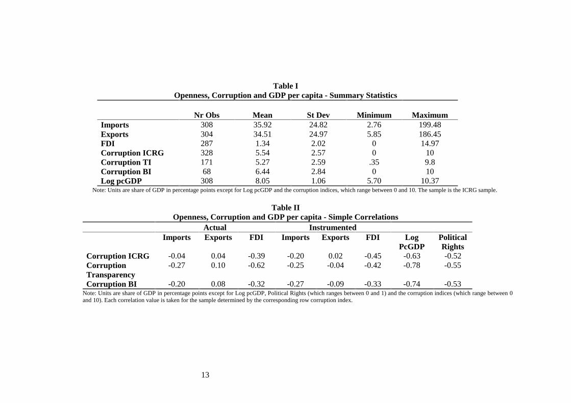
Tables I and II present summary statistics and simple correlationcoefficients for the openness indicators, the three corruption indices, the log ofper capita GDP and the level of political rights. We also present the correlationbetween each instrumented openness indicator and the rest of the variables.Imports as a share of GDP ranges from 2.76 to 199 whereas exports fluctuatebetween 5.85 and 186 percent of GDP. Foreign direct investment inflows varyin a much shorter range, between 0 and roughly 15 percent of GDP. Thecorruption indices have all been transformed so that they range from 0 (lowestcorruption) to 10 (highest corruption). Thus, an increase in the corruptionindex corresponds to a decrease in corruption. The standard deviation of eachopenness variable is useful in evaluating the extent to which each can be usedas an instrument to decrease corruption. In particular, we will be interested inthe relative magnitude of feasible changes in import intensity as compared tochanges in FDI and the level of GDP per capita. In Table III it can be shownthat lower levels of corruption are weakly correlated with imports and exports(respectively negatively and positively) and display a stronger negativecorrelation with FDI inflows. Furthermore, the correlation of instrumented

22 In the same way as before, as one of the large economies increases its imports/FDIoutflows, we assume that this is likely to positively affect the exports/FDI inflows of allcountries which are closer, share a land border, a common language or a common religion.

12

export intensity with corruption decreases to levels very close to 0, whereasinstrumented imports and FDI remain negatively correlated with corruption.

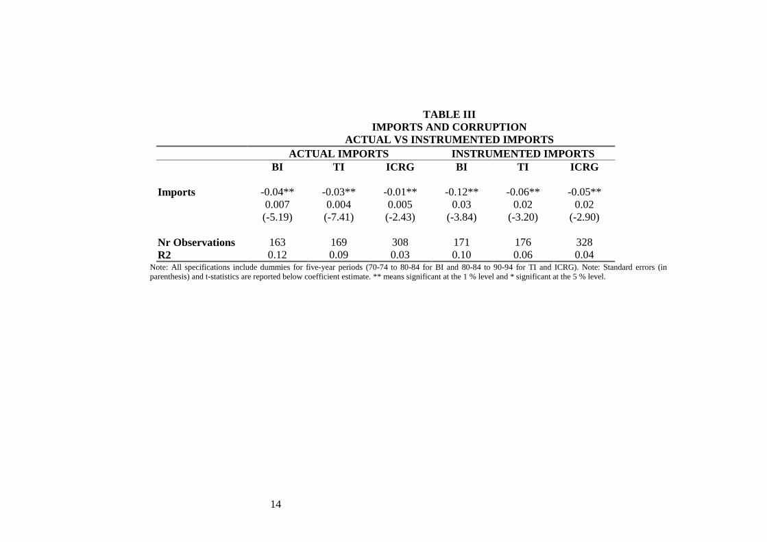
Tables II through V present the estimates for the effect of imports onthe level of corruption. In Table III we present Pooled Least Squares estimatesof corruption on import intensity alone, both the actual variable and theinstrumented variable.23 Actual import intensity is negatively and significantlyrelated to corruption, whatever the indicator used. As we can verify,instrumented import intensity remains a significant determinant of thecorruption but the size of the effect is larger than that on actual imports, a signthat the instrument is capturing an actual relationship.24 As shown by the R2,import intensity alone explains an important share of the variability ofcorruption.

23 In all specifications dummies for each five-year period are added to correct for time-varyingaverage levels of corruption.24 When income per capita is used as a control actual import intensity becomes insignificant inthe case of ICRG, whereas instrumented import intensity remains significant throughout. Thispattern is repeated with other controls added so that instrumented imports is fairly robust tospecification whereas actual imports is not.

13

Table IOpenness, Corruption and GDP per capita - Summary Statistics

Nr Obs Mean St Dev Minimum MaximumImports 308 35.92 24.82 2.76 199.48Exports 304 34.51 24.97 5.85 186.45FDI 287 1.34 2.02 0 14.97Corruption ICRG 328 5.54 2.57 0 10Corruption TI 171 5.27 2.59 .35 9.8Corruption BI 68 6.44 2.84 0 10Log pcGDP 308 8.05 1.06 5.70 10.37

Note: Units are share of GDP in percentage points except for Log pcGDP and the corruption indices, which range between 0 and 10. The sample is the ICRG sample.

Table IIOpenness, Corruption and GDP per capita - Simple Correlations

Actual InstrumentedImports Exports FDI Imports Exports FDI Log

PcGDPPoliticalRights

Corruption ICRG -0.04 0.04 -0.39 -0.20 0.02 -0.45 -0.63 -0.52CorruptionTransparency

-0.27 0.10 -0.62 -0.25 -0.04 -0.42 -0.78 -0.55

Corruption BI -0.20 0.08 -0.32 -0.27 -0.09 -0.33 -0.74 -0.53Note: Units are share of GDP in percentage points except for Log pcGDP, Political Rights (which ranges between 0 and 1) and the corruption indices (which range between 0and 10). Each correlation value is taken for the sample determined by the corresponding row corruption index.

14

TABLE IIIIMPORTS AND CORRUPTION

ACTUAL VS INSTRUMENTED IMPORTSACTUAL IMPORTS INSTRUMENTED IMPORTS

BI TI ICRG BI TI ICRG

Imports -0.04** -0.03** -0.01** -0.12** -0.06** -0.05**0.007 0.004 0.005 0.03 0.02 0.02(-5.19) (-7.41) (-2.43) (-3.84) (-3.20) (-2.90)

Nr Observations 163 169 308 171 176 328R2 0.12 0.09 0.03 0.10 0.06 0.04

Note: All specifications include dummies for five-year periods (70-74 to 80-84 for BI and 80-84 to 90-94 for TI and ICRG). Note: Standard errors (inparenthesis) and t-statistics are reported below coefficient estimate. ** means significant at the 1 % level and * significant at the 5 % level.

15

TABLE IVIMPORTS AND CORRUPTION

POOLED OLS, FIXED AND RANDOM EFFECTS ESTIMATES

POOLED LEAST SQUARES FIXEDEFFECTS

RANDOMEFFECTS

BI TI ICRG BI TI ICRG BI TI ICRG

Imports -0.07** -0.03** -0.03** -0.04 -0.02 0.02 -0.07** -0.03** -0.020.02 0.01 0.01 0.09 0.05 0.04 0.03 0.02 0.02-3.31 -2.85 -2.33 -0.43 -0.45 0.62 -2.09 -2.10 -1.09

GDP Per Capita -1.70** -2.09** -1.21** 0.13 -0.90 1.09** -1.61** -1.83** -0.85**0.31 0.20 0.13 1.26 0.75 0.45 0.33 0.20 0.17-5.43 10.38 9.44 0.10 -1.21 2.44 -4.85 -8.97 -4.88

Political Rights -1.69** 0.56** -1.51** -0.77 -0.08 -0.62 -1.20 -0.10 -1.30**0.88 0.63 0.36 1.21 0.69 0.48 0.80 0.53 0.41-1.92 0.88 -4.19 -0.63 -0.12 -1.29 -1.50 -0.19 -3.20

Nr Observations 170 171 308 170 171 308 170 171 308R2 0.47 0.63 0.46 0.21 0.04 0.12 0.47 0.62 0.46Note: All specifications include dummies for five-year periods (70-74 to 80-84 for BI and 80-84 to 90-94 for TI and ICRG). Note: Standard errors (in parenthesis) and t-statistics are reported below coefficient estimate. ** means significant at the 1 % level and * significant at the 5 % level.

16

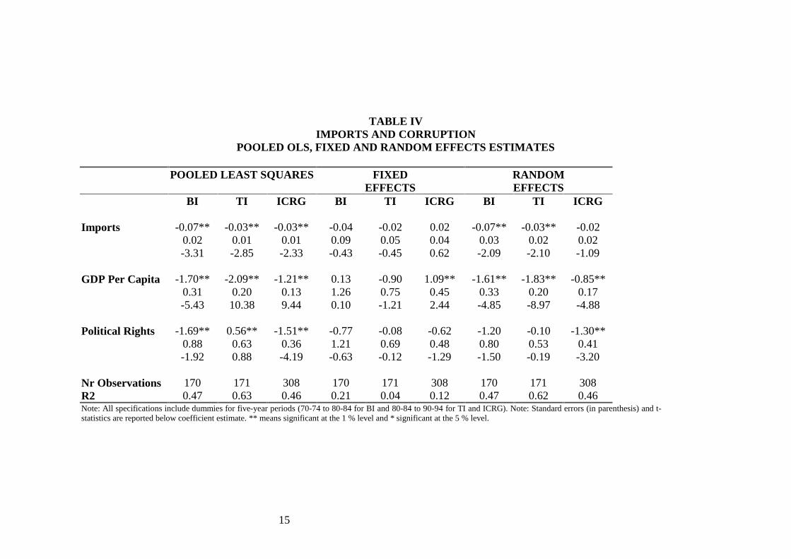
Table IV presents Pooled LS, Fixed Effects and Random Effectsestimates of the basic specification of the determinants of corruption, withincome per capita and political rights as controls. As can be verified,instrumented imports appears with a significant and negative sign in all butone of the Pooled Least Squares or the Random Effects estimations.

This is indicative of higher openness to imports causing a decrease incorruption. The size of the coefficient on imports is such that a 10 percentincrease in import intensity leads to a 0.6 decrease in the corruption index (1.4decrease in the BI sample) out of a total range of 10. A standard deviationincrease in import share (approximately 25) leads to a 1.5 decrease incorruption. This is an effect of similar magnitude to the effect of a onestandard deviation in GDP per capita (approximately 1). In other words,openness is a statistically and economically significant determinant ofcorruption when the cross-section variation is used in the estimates.

In contrast, instrumented import intensity is never significant when welook at fixed effects estimates and thus control for any unchanging countrycharacteristic. The time dimension of the variability in import intensity seemsto be unimportant in explaining corruption. It is the fact that a country isgeographically and culturally close close to, say, the United States, togetherwith the fact that the US is a big exporter, that decreases corruption, not thequinquennial variability in US exports. The insignificant sign on per capitaGDP for the BI and TI indices and the lower share of total variation in thecorruption index that is explained point to the possibility that the Fixed Effectsspecification is not the appropriate one. It may be what one would expectgiven the relative stability of the indices of corruption across time for the samecountry. However, for the first time, with the use of time varying instruments,we show that previous work, which relies on the cross-section variation, isappropriate.

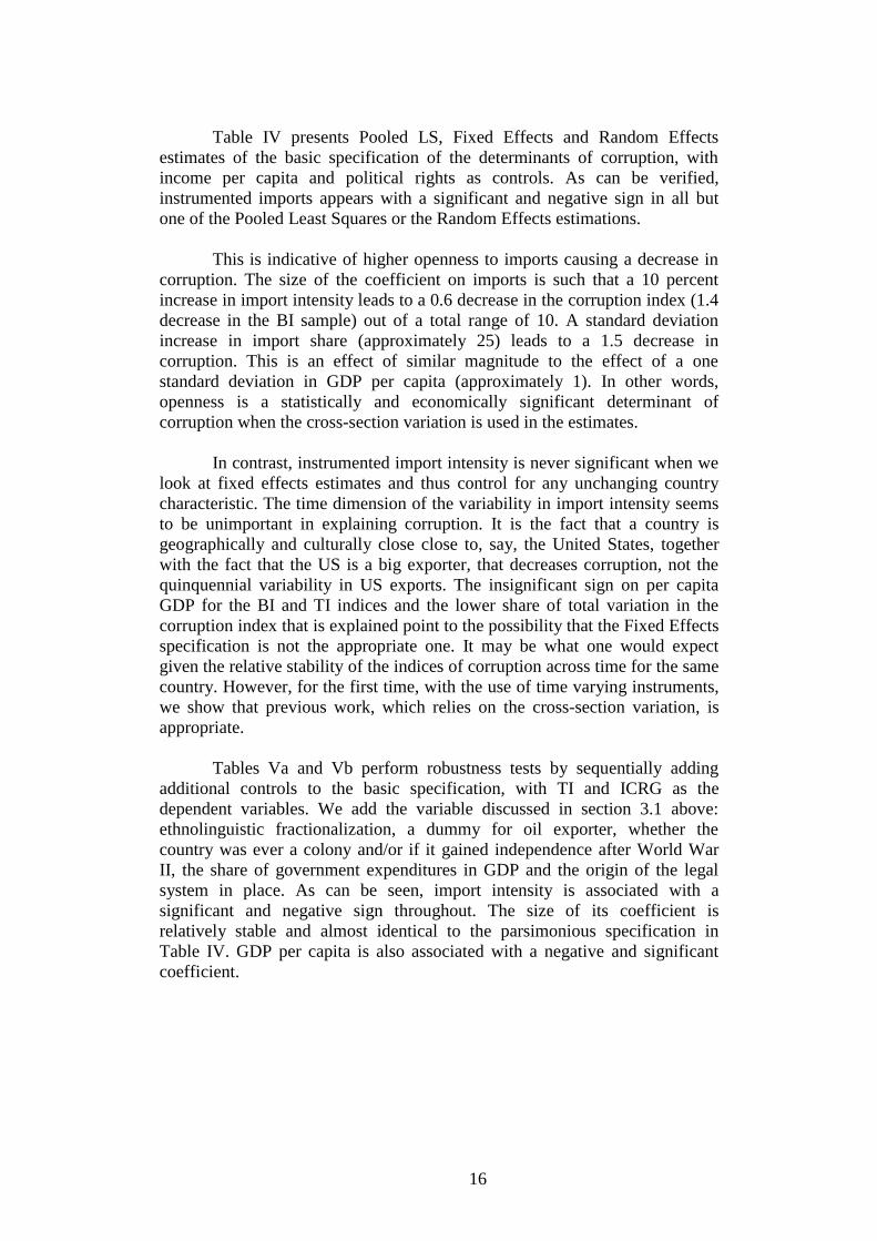
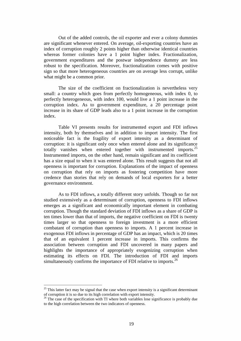
Tables Va and Vb perform robustness tests by sequentially addingadditional controls to the basic specification, with TI and ICRG as thedependent variables. We add the variable discussed in section 3.1 above:ethnolinguistic fractionalization, a dummy for oil exporter, whether thecountry was ever a colony and/or if it gained independence after World WarII, the share of government expenditures in GDP and the origin of the legalsystem in place. As can be seen, import intensity is associated with asignificant and negative sign throughout. The size of its coefficient isrelatively stable and almost identical to the parsimonious specification inTable IV. GDP per capita is also associated with a negative and significantcoefficient.

17

TABLE VaIMPORTS AND CORRUPTION - ICRG

POOLED LEAST SQUARES

(1) (2) (3) (4) (5) (6) (7)

Imports -0.03** -0.05** -0.04** -0.03** -0.03** -0.03** -0.03**0.01 0.01 0.01 0.01 0.01 0.01 0.01-2.33 -4.62 -4.33 -3.15 -2.85 -2.63 -2.71

GDP Per Capita -1.21** -1.43** -1.70** -1.46** -1.47** -1.60** -1.47**0.13 0.16 0.16 0.18 0.18 0.19 0.19-9.44 -8.76 -10.84 -7.98 -7.94 -8.39 -7.85

Political Rights -1.51** -1.42** -0.58 -0.51 -0.55 -0.72* -0.460.36 0.41 0.40 0.39 0.40 0.41 0.46-4.19 -3.47 -1.44 -1.30 -1.36 -1.77 -1.00

Fractionalization -0.01* -0.01** -0.01** -0.01* -0.01** -0.01**0.01 0.00 0.00 0.01 0.01 0.01-1.78 -2.27 -2.19 -1.89 -1.96 -1.71

Oil Exporter 2.08** 2.00** 2.01** 1.92** 1.69**0.33 0.33 0.33 0.34 0.346.22 6.06 6.09 5.61 4.94

Ever a Colony 1.09** 1.15** 1.13** 0.81**0.28 0.31 0.31 0.333.87 3.65 3.62 2.47

Postwar Independence -0.14 -0.09 0.210.34 0.33 0.37-0.43 -0.28 0.56

Government Expenditure -0.05** -0.04*1.85 1.95-2.68 -1.920.01 0.06

Legal System Dummies No No No No No No YesPeriod Dummies Yes Yes Yes Yes Yes Yes Yes

Nr Observations 308 280 280 280 280 278 278R2 0.46 0.52 0.56 0.58 0.58 0.60 0.61Note: All specifications include dummies for five-year periods (70-74 to 80-84 for BI and 80-84 to 90-94 for TI andICRG). Note: Standard errors (in parenthesis) and t-statistics are reported below coefficient estimate. ** Meanssignificant at the 1 % level and * significant at the 5 % level.

18

TABLE VbIMPORTS AND CORRUPTION - TI

POOLED LEAST SQUARES

(1) (2) (3) (4) (5) (6) (7)

Imports -0.03** -0.06** -0.05** -0.06** -0.06** -0.05** -0.06**0.01 0.01 0.01 0.01 0.01 0.01 0.01-2.85 -4.94 -4.38 -5.41 -4.83 -4.59 -5.51

GDP Per Capita -2.09** -2.32** -2.29** -2.50** -2.59** -2.73** -2.32**0.20 0.23 0.22 0.21 0.20 0.20 0.21

-10.38 -10.28 -10.55 -11.63 -12.84 -13.44 -11.25

Political Rights 0.56 0.81 0.82 0.48 0.13 -0.07 0.360.63 0.66 0.64 0.63 0.63 0.61 0.590.88 1.22 1.29 0.76 0.20 -0.12 0.60

Fractionalization -0.01* -0.01** -0.01** -0.01 -0.01* -0.000.01 0.01 0.01 0.01 0.01 0.01-1.81 -1.83 -2.12 -1.55 -1.79 -0.36

Oil Exporter 2.63** 2.87** 2.92** 2.73** 2.03**0.28 0.37 0.31 0.34 0.419.40 7.82 9.45 7.92 4.96

Ever a Colony -0.97** -0.74** -0.74** -0.85**0.30 0.31 0.31 0.34-3.28 -2.39 -2.40 -2.52

Postwar Independence -0.95** -0.87** -0.290.36 0.37 0.35-2.63 -2.39 -0.84

Government Expenditure -0.06** -0.022.04 1.90-3.06 -1.18

Legal System Dummies No No No No No No YesPeriod Dummies Yes Yes Yes Yes Yes Yes Yes

Nr Observations 308 280 280 280 280 278 278R2 0.46 0.52 0.56 0.58 0.58 0.60 0.61Note: All specifications include dummies for five-year periods (70-74 to 80-84 for BI and 80-84 to 90-94 for TI andICRG). Note: Standard errors (in parenthesis) and t-statistics are reported below coefficient estimate. ** meanssignificant at the 1 % level and * significant at the 5 % level.

19

Out of the added controls, the oil exporter and ever a colony dummiesare significant whenever entered. On average, oil-exporting countries have anindex of corruption roughly 2 points higher than otherwise identical countrieswhereas former colonies have a 1 point higher index. Fractionalization,government expenditures and the postwar independence dummy are lessrobust to the specification. Moreover, fractionalization comes with positivesign so that more heterogeneous countries are on average less corrupt, unlikewhat might be a common prior.

The size of the coefficient on fractionalization is nevertheless verysmall: a country which goes from perfectly homogeneous, with index 0, toperfectly heterogeneous, with index 100, would live a 1 point increase in thecorruption index. As to government expenditure, a 20 percentage pointincrease in its share of GDP leads also to a 1 point increase in the corruptionindex.

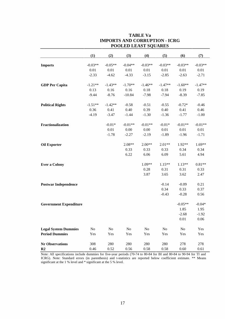
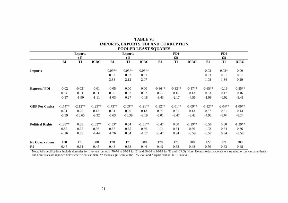
Table VI presents results for instrumented export and FDI inflowsintensity, both by themselves and in addition to import intensity. The firstnoticeable fact is the fragility of export intensity as a determinant ofcorruption: it is significant only once when entered alone and its significancetotally vanishes when entered together with instrumented imports.25

Instrumented imports, on the other hand, remain significant and its coefficienthas a size equal to when it was entered alone. This result suggests that not allopenness is important for corruption. Explanations of the impact of opennesson corruption that rely on imports as fostering competition have morecredence than stories that rely on demands of local exporters for a bettergovernance environment.

As to FDI inflows, a totally different story unfolds. Though so far notstudied extensively as a determinant of corruption, openness to FDI inflowsemerges as a significant and economically important element in combatingcorruption. Though the standard deviation of FDI inflows as a share of GDP isten times lower than that of imports, the negative coefficient on FDI is twentytimes larger so that openness to foreign investment is a more efficientcombatant of corruption than openness to imports. A 1 percent increase inexogenous FDI inflows in percentage of GDP has an impact, which is 20 timesthat of an equivalent 1 percent increase in imports. This confirms theassociation between corruption and FDI uncovered in many papers andhighlights the importance of appropriately exogenizing corruption whenestimating its effects on FDI. The introduction of FDI and importssimultaneously confirms the importance of FDI relative to imports.26

25 This latter fact may be signal that the case when export intensity is a significant determinantof corruption it is so due to its high correlation with export intensity.26 The case of the specification with TI where both variables lose significance is probably dueto the high correlation between the two indicators of openness.

21

TABLE VIIMPORTS, EXPORTS, FDI AND CORRUPTION

POOLED LEAST SQUARESExports

(1)Exports

(1)FDI(2)

FDI(3)

BI TI ICRG BI TI ICRG BI TI ICRG BI TI ICRG

Imports 0.09** 0.03** 0.03** 0.03 0.03* 0.000.02 0.02 0.01 0.03 0.01 0.013.88 2.12 2.07 1.08 1.84 0.29

Exports / FDI -0.02 -0.03* -0.01 -0.05 0.00 0.00 -0.86** -0.33** -0.57** -0.65** -0.16 -0.55**0.04 0.01 0.01 0.05 0.02 0.02 0.25 0.15 0.13 0.33 0.17 0.16-0.57 -1.90 -1.11 -1.03 0.27 -0.18 -3.43 -2.17 -4.55 -1.98 -0.92 -3.41

GDP Per Capita -1.74** -2.12** -1.23** -1.73** -2.09** -1.21** -1.82** -2.01** -1.09** -1.82** -2.04** -1.09**0.31 0.20 0.13 0.31 0.20 0.13 0.36 0.21 0.13 0.37 0.21 0.13-5.59 -10.65 -9.32 -5.63 -10.39 -9.19 -5.01 -9.47 -8.42 -4.92 -9.64 -8.24

Political Rights -1.88** 0.39 -1.62** -1.53* 0.54 -1.51** -0.47 0.60 -1.29** -0.58 0.60 -1.29**0.87 0.62 0.36 0.87 0.65 0.36 1.01 0.64 0.36 1.02 0.64 0.36-2.16 0.63 -4.44 -1.76 0.84 -4.17 -0.47 0.94 -3.59 -0.57 0.94 -3.59

Nr Observations 170 171 308 170 171 308 170 171 308 122 171 308R2 0.45 0.61 0.45 0.48 0.63 0.46 0.49 0.62 0.48 0.50 0.63 0.48

Note: All specifications include dummies for five-year periods (70-74 to 80-84 for BI and 80-84 to 90-94 for TI and ICRG). Note: Heteroskedastic-consistent standard errors (in parenthesis)and t-statistics are reported below coefficient estimate. ** means significant at the 5 % level and * significant at the 10 % level.

22

In sum, this section highlights the importance of country openness tocorruption by using new and powerful instruments for openness. Higherexogenous import intensity and, specially, FDI intensity, lead to significantlylower levels of corruption. Export intensity, on the other hand, does not seemto cause a decrease in the level of corruption. Future work should exploitfurther the role of FDI in fighting corruption.

4.2. Are Tariffs All That Matters?

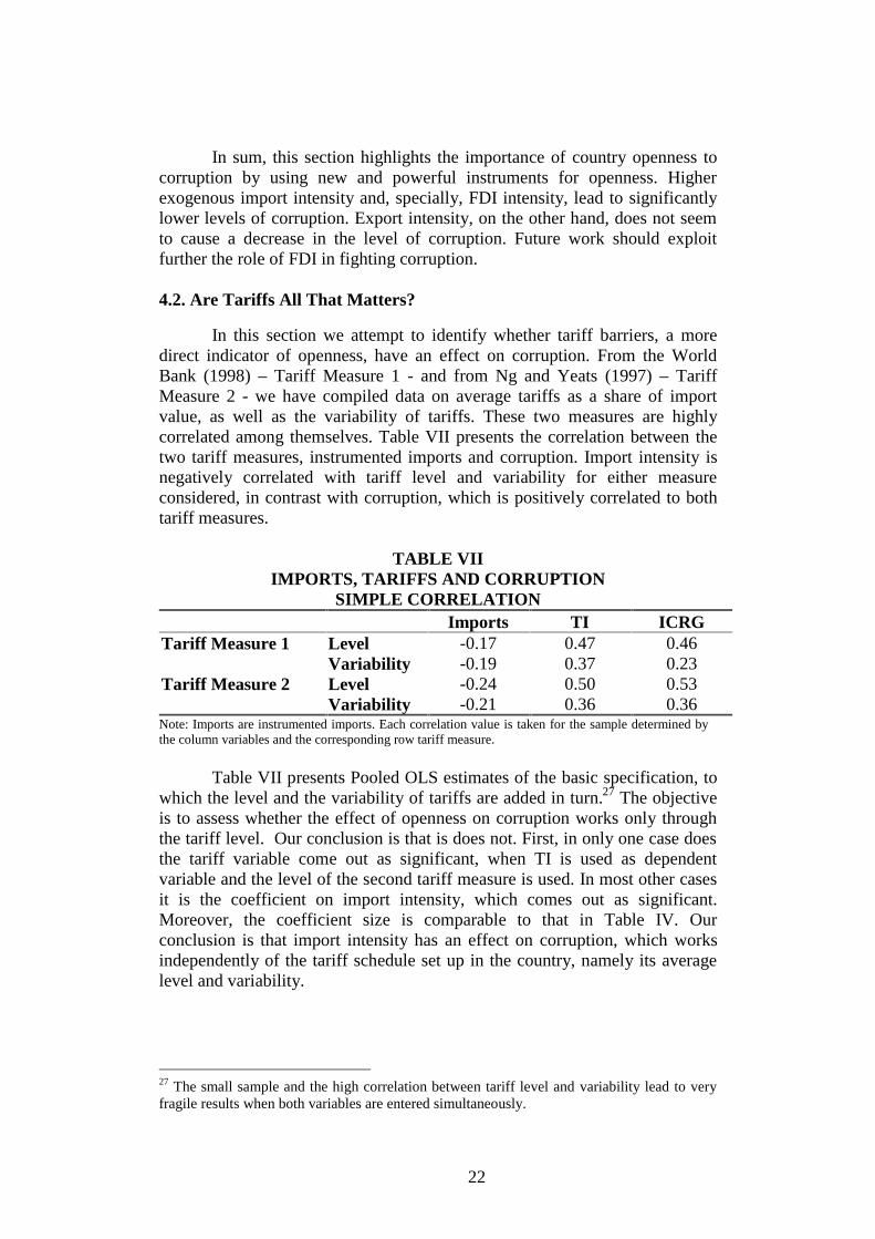
In this section we attempt to identify whether tariff barriers, a moredirect indicator of openness, have an effect on corruption. From the WorldBank (1998) – Tariff Measure 1 - and from Ng and Yeats (1997) – TariffMeasure 2 - we have compiled data on average tariffs as a share of importvalue, as well as the variability of tariffs. These two measures are highlycorrelated among themselves. Table VII presents the correlation between thetwo tariff measures, instrumented imports and corruption. Import intensity isnegatively correlated with tariff level and variability for either measureconsidered, in contrast with corruption, which is positively correlated to bothtariff measures.

TABLE VIIIMPORTS, TARIFFS AND CORRUPTION

SIMPLE CORRELATIONImports TI ICRG

Tariff Measure 1 Level -0.17 0.47 0.46Variability -0.19 0.37 0.23Level -0.24 0.50 0.53Tariff Measure 2Variability -0.21 0.36 0.36

Note: Imports are instrumented imports. Each correlation value is taken for the sample determined bythe column variables and the corresponding row tariff measure.

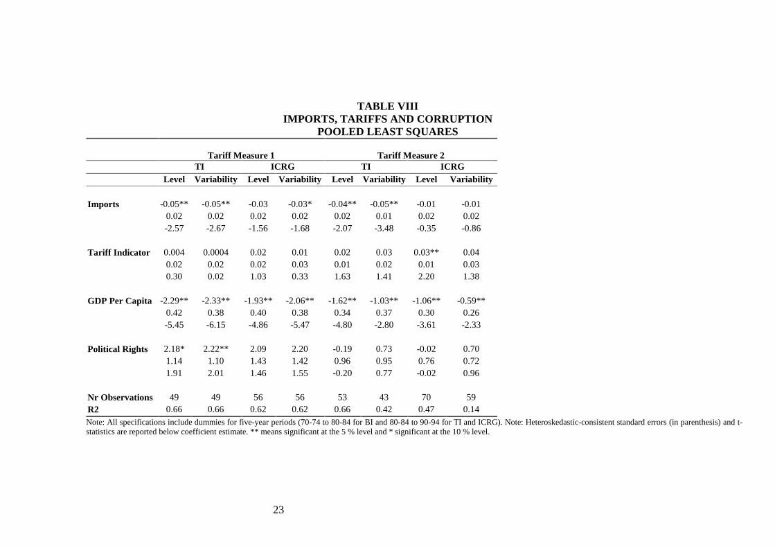
Table VII presents Pooled OLS estimates of the basic specification, towhich the level and the variability of tariffs are added in turn.27 The objectiveis to assess whether the effect of openness on corruption works only throughthe tariff level. Our conclusion is that is does not. First, in only one case doesthe tariff variable come out as significant, when TI is used as dependentvariable and the level of the second tariff measure is used. In most other casesit is the coefficient on import intensity, which comes out as significant.Moreover, the coefficient size is comparable to that in Table IV. Ourconclusion is that import intensity has an effect on corruption, which worksindependently of the tariff schedule set up in the country, namely its averagelevel and variability.

27 The small sample and the high correlation between tariff level and variability lead to veryfragile results when both variables are entered simultaneously.

23

TABLE VIIIIMPORTS, TARIFFS AND CORRUPTION

POOLED LEAST SQUARES

Tariff Measure 1 Tariff Measure 2TI ICRG TI ICRG

Level Variability Level Variability Level Variability Level Variability

Imports -0.05** -0.05** -0.03 -0.03* -0.04** -0.05** -0.01 -0.010.02 0.02 0.02 0.02 0.02 0.01 0.02 0.02-2.57 -2.67 -1.56 -1.68 -2.07 -3.48 -0.35 -0.86

Tariff Indicator 0.004 0.0004 0.02 0.01 0.02 0.03 0.03** 0.040.02 0.02 0.02 0.03 0.01 0.02 0.01 0.030.30 0.02 1.03 0.33 1.63 1.41 2.20 1.38

GDP Per Capita -2.29** -2.33** -1.93** -2.06** -1.62** -1.03** -1.06** -0.59**0.42 0.38 0.40 0.38 0.34 0.37 0.30 0.26-5.45 -6.15 -4.86 -5.47 -4.80 -2.80 -3.61 -2.33

Political Rights 2.18* 2.22** 2.09 2.20 -0.19 0.73 -0.02 0.701.14 1.10 1.43 1.42 0.96 0.95 0.76 0.721.91 2.01 1.46 1.55 -0.20 0.77 -0.02 0.96

Nr Observations 49 49 56 56 53 43 70 59R2 0.66 0.66 0.62 0.62 0.66 0.42 0.47 0.14Note: All specifications include dummies for five-year periods (70-74 to 80-84 for BI and 80-84 to 90-94 for TI and ICRG). Note: Heteroskedastic-consistent standard errors (in parenthesis) and t-statistics are reported below coefficient estimate. ** means significant at the 5 % level and * significant at the 10 % level.

24

This suggests direct effects of import intensity on the competitivenessof the local markets rather than the potential of high and variable tariffs togenerate rent-seeking behavior and corruption.28

4.3. Are All Imports Alike? Sectoral Imports and Corruption

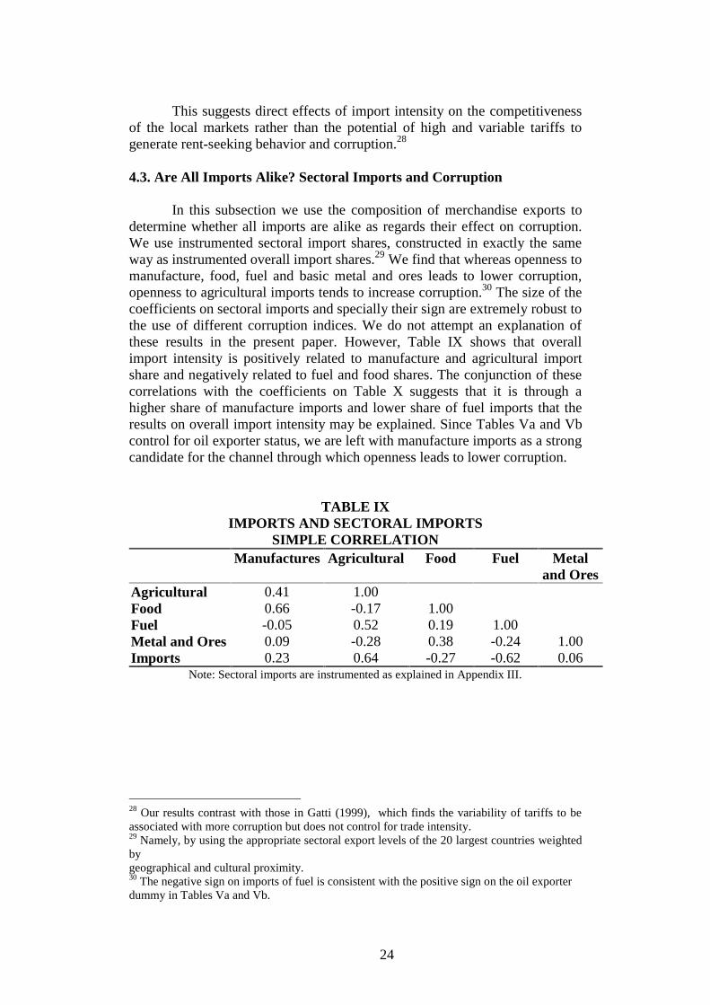
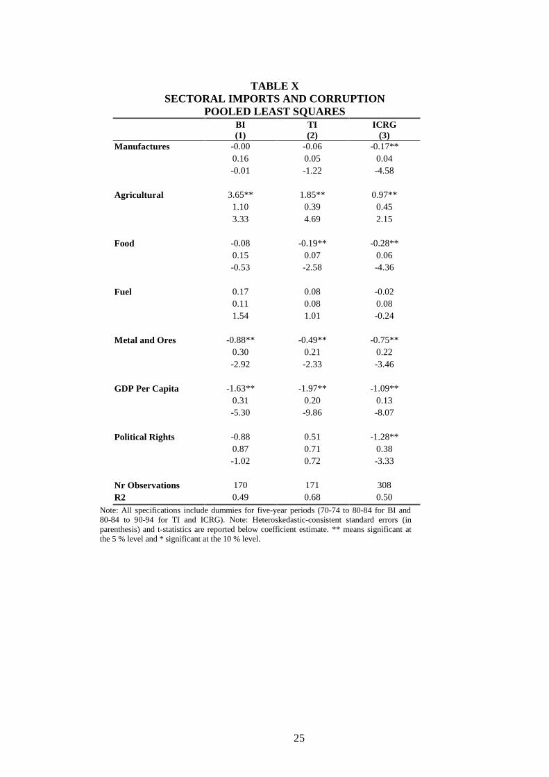
In this subsection we use the composition of merchandise exports todetermine whether all imports are alike as regards their effect on corruption.We use instrumented sectoral import shares, constructed in exactly the sameway as instrumented overall import shares.29 We find that whereas openness tomanufacture, food, fuel and basic metal and ores leads to lower corruption,openness to agricultural imports tends to increase corruption.30 The size of thecoefficients on sectoral imports and specially their sign are extremely robust tothe use of different corruption indices. We do not attempt an explanation ofthese results in the present paper. However, Table IX shows that overallimport intensity is positively related to manufacture and agricultural importshare and negatively related to fuel and food shares. The conjunction of thesecorrelations with the coefficients on Table X suggests that it is through ahigher share of manufacture imports and lower share of fuel imports that theresults on overall import intensity may be explained. Since Tables Va and Vbcontrol for oil exporter status, we are left with manufacture imports as a strongcandidate for the channel through which openness leads to lower corruption.

TABLE IXIMPORTS AND SECTORAL IMPORTS

SIMPLE CORRELATIONManufactures Agricultural Food Fuel Metal

and OresAgricultural 0.41 1.00Food 0.66 -0.17 1.00Fuel -0.05 0.52 0.19 1.00Metal and Ores 0.09 -0.28 0.38 -0.24 1.00Imports 0.23 0.64 -0.27 -0.62 0.06

Note: Sectoral imports are instrumented as explained in Appendix III.

28 Our results contrast with those in Gatti (1999), which finds the variability of tariffs to beassociated with more corruption but does not control for trade intensity.29 Namely, by using the appropriate sectoral export levels of the 20 largest countries weightedbygeographical and cultural proximity.30 The negative sign on imports of fuel is consistent with the positive sign on the oil exporterdummy in Tables Va and Vb.

25

TABLE XSECTORAL IMPORTS AND CORRUPTION

POOLED LEAST SQUARESBI(1)

TI(2)

ICRG(3)

Manufactures -0.00 -0.06 -0.17**0.16 0.05 0.04-0.01 -1.22 -4.58

Agricultural 3.65** 1.85** 0.97**1.10 0.39 0.453.33 4.69 2.15

Food -0.08 -0.19** -0.28**0.15 0.07 0.06-0.53 -2.58 -4.36

Fuel 0.17 0.08 -0.020.11 0.08 0.081.54 1.01 -0.24

Metal and Ores -0.88** -0.49** -0.75**0.30 0.21 0.22-2.92 -2.33 -3.46

GDP Per Capita -1.63** -1.97** -1.09**0.31 0.20 0.13-5.30 -9.86 -8.07

Political Rights -0.88 0.51 -1.28**0.87 0.71 0.38-1.02 0.72 -3.33

Nr Observations 170 171 308R2 0.49 0.68 0.50

Note: All specifications include dummies for five-year periods (70-74 to 80-84 for BI and80-84 to 90-94 for TI and ICRG). Note: Heteroskedastic-consistent standard errors (inparenthesis) and t-statistics are reported below coefficient estimate. ** means significant atthe 5 % level and * significant at the 10 % level.

26

5- Conclusions

This paper makes a systematic attempt to estimate the effects ofopenness on corruption. The impact of corruption on variables such as foreigndirect investment has been relatively well studied. The reverse causality,however, which analyzes the effect of openness on corruption remains an issueof policy debate. We estimate the effects of higher levels of imports, exportsand foreign direct investment inflows (as shares of Gross Domestic Product)on corruption. To address the causality issue we develop and use powerfulinstruments, variable across country and time, which correct for reversecausation.

Several important results arise. First, imports are an important channelthrough which openness to the international economy leads to lowercorruption. This result is robust to the inclusion of several determinants ofcorruption studied in the literature. There is an association between actualimport intensity and the level of corruption but when we instrument for importintensity the effect is more robust and quantitatively stronger. The powerfulinstruments used indicate that imports are not only associated with lesscorruption but also reduce corruption. Interestingly, given the typical deviationof import intensity in the sample, the effect of openness indicators oncorruption is of the same magnitude as that of income per capita on corruption.This is important since a policy of trade openness is more easily pursued thana general policy of raising the economy’s average income.

Second, export intensity seems to be only weakly associated withcorruption whereas the intensity of foreign direct investment inflows is astatistically and economically significant determinant of corruption. More FDIleads to lower corruption and its effect is stronger than that of imports. A 2percent increase in FDI leads to around 1.5 decrease in the country corruptionindex, out of a total possible range of 10. Third, the effect of imports inlowering corruption does not work through the tariff schedule. Moreover, thelevel and variability of tariffs does not impact corruption significantly afterimport intensity is taken into account. Fourth, a higher intensity of imports ofmanufactures, food, fuel and metal and ores lower corruption, whereasagricultural imports increase corruption.

The results of this paper strongly point to a beneficial effect of countryopenness on corruption. Our evidence shows that higher levels of opennessreduce corruption, thus adding another argument for trade and FDIliberalization policies. More needs to be done in analyzing the channelsthrough which openness decreases corruption but our evidence suggests thatcompetition in the goods and assets markets both contribute to detercorruption.

27

References

- Ades, Alberto, and Rafael DiTella (1997), “The New Economics of Corruption: A Surveyand Some New Results,” Political Studies, Summer 1997, Vol. 45, N 3, pp. 496-516.

- Ades, Alberto and Rafael DiTella (1999), “Rents, Competition and Corruption,” forthcomingThe American Economic Review.

- Bardhan, Pranab (1997), "Corruption and Development: A Review of Issues", Journal ofEconomic Literature, 35, 1320-1346.

- Bhagwati, Jagdish (1982), Directly Unproductive, Profit-Seeking (DUP) Activities” , Journalof Political Economy, 90, 988-1002.

- Bhagwati, Jagdish and T. N. Srinivasan (1980), “Revenue Seeking: A Generalization of theTheory of Tariffs”, Journal of Political Economy, 88, 1069-87.

- Bliss, Christopher and Rafael DiTella (1997), “Does Competition Kill Corruption?,” Journalof Political Economy, October, Vol 105, N 5, 1001-23.

- Brock, William and Stephen Magee (1978), “ The economics of Special Interest Politics: theCase of the Tariff”, American Economic Review Papers and Proceedings, 68, 246-50.

- Frankel, Jeffrey, Ernesto Stein and Shang-Jin Wei (1993), “Continental Trading Blocs: AreThey Natural, or Super-Natural?”, NBER Working Paper No. W4588

- Gatti, Roberta (1999), “Corruption and Trade Tariffs, or a Case for Uniform Tariffs”, WorldBank Working Paper.

- Helpman, Elhanan (1995), “ Politics and Trade Policy”, NBER Working Papers 5309.

- Hines, James (1995), “Forbidden Payment: Foreign Bribery and American Business”, NBERWorking Papers 5266, Cambridge.

- Kaufmann, Daniel and Shang-Jin Wei (1999), “Does ’Grease Money’ Speed Up the Wheelsof Commerce?”, NBER Working Paper 7093.

- Keefer, Philip and Stephen Knack (1995), "Institutions and Economic Performance: Cross-Country Tests Using Alternative Institutional Measures", Economics and Politics, 7,November 207-227.

- Kennedy, Peter (1998), “A Guide to Econometrics”, MIT Press.

- Kimberley, Ann (ed.) (1997), "Corruption and the Global Economy", Institute forInternational Economics, Washington, DC.

- Klitgaard, Robert (1988), “Controlling corruption”, Berkeley and London: University ofCalifornia Press, 1988.

- Krueger, Anne (1974), “The Political Economy of the Rent Seeking Society”, AmericanEconomic Review 64, no. 3, June, p. 291-303.

- LaPorta, Rafael, Florencio Lopez de Silanes, Andrei Shleifer and Robert Vishny, (1998),“The Quality of Government”, NBER Working Paper 6727.

28

- Leite, C., and Weidmann, J. (1999), “Does Mother Nature Corrupt? Natural Resources,Corruption and Economic Growth”, International Monetary Fund Working Paper, WashingtonDC.

- Leff, Nathaniel (1964), “Economic Development through Bureaucratic Corruption”,American Behavioral Scientist, 8-14.

- Loayza, Norman (1996), “The Economics of the Informal Sector: A Simple Model and SomeEmpirical Evidence from Latin America”, The World Bank, Washington DC.

- Mauro, Paolo (1995), “ Corruption and Growth”, Quarterly Journal of Economics, 110.

- Mauro, Paolo (1998), “ Corruption and the Composition of Government Expenditure”,Journal of Public Economics, 69, p. 263-279.

- Mauro, Paolo (1996), “ The Effects of Corruption on Growth, Investment and GovernmentExpenditure”, Corruption and Growth”, IMF Working Papers, IMF, Washington DC.

- Murphy, Kevin, Andrei Shleifer and Robert Vishny (1991), “Allocation of Talent:Implications for Growth”, Quarterly Journal Of Economics, 106.

- Ng, Francis and Alexander Yeats (1997), “Open Economies Work Better! Did Africa’sProtectionist Policies Cause its Marginalization in World Trade”, World Bank Working Paper,The World Bank, Washington D.C.

- Rose-Ackerman, Susan (1975), “The Economics of Corruption”, Journal of PublicEconomics, 4, 187-203.

- Rose-Ackerman, Susan (1978), “Corruption: A Study in Political Economy”, New York,Academic Press.

- Rose-Ackerman, Susan (1988), “Bribery”, in The New Palgrave Dictionary of EconomicThought, edited by John Eatwell, Murray Milgate and Peter Newman, London, Macmillan.

- Sachs, Jeffrey and Andrew Warner (1995), " Natural Resource Abundance and EconomicGrowth", HIID Development Discussion Paper No. 517, Harvard University.

- Shleifer, Andrei and Robert Vishny (1993), “Corruption”, Quarterly Journal Of Economics,108, p. 599-617.

- Shleifer, Andrei and Robert Vishny (1994), “Politicians and Firms”, Quarterly Journal OfEconomics, 109, p. 995-1025.

- Summers, Robert and Alan Heston (1991), "The Penn World Table (Mark 5): An ExpandedSet of International Comparisons, 1950-1988", Quarterly Journal of Economics, 106(2), May,327-68.

- Tanzi, Vito (1994), “Corruption, Governmental Activities and Markets”, IMF WorkingPapers 94/99, IMF, Washington DC.

- Tanzi, Vito and Hamid Davoodi (1997), “Corruption, Public Investment, and Growth”, IMFWorking Papers, IMF, Washington DC.

- Tanzi, Vito (1998), “Corruption Around the World - Causes, Consequences, Scope, andCures” , IMF Working Papers, IMF, Washington DC.

- Tornell, Aaron and Philip Lane (1998), “Voracity and Growth”, American EconomicReview, forthcoming.

29

- Tullock, Gordon (1967), “The Welfare Costs of Tariffs, Monopolies and Theft”, WesternEconomic Journal, 5, 224-32.

- Wei, Shang-Jin (1997a), "How Taxing is Corruption on International Investors?", NBERWorking Paper No. 6030.

- Wei, Shang-Jin (1997b), "Why is Corruption So Much More Taxing Than Tax?Arbitrariness Kills", mimeo, Harvard University.

- Wei, Shang-Jin (2000), “Natural Openness and Good Government”, NBER Working Paper7765, Cambridge, MA.

- World Bank (1998), “World Development Indicators”, World Bank, Washington DC.

30

Appendix IData Sources and Definitions

Imports - Source: World Bank (1998). Definition: Imports as a share of economy’s GDP. Unit: Percent.

Exports - Source: World Bank (1998). Definition: Imports as a share of economy’s GDP. Unit: Percent.

Foreign Direct Investment- Source: World Bank (1998). Definition: Gross inflows of foreign directinvestment as a share of domestic economy’s GDP. Unit: Percent.

Tariff Barriers - World Bank (1998) and Ng and Yeats (1997). Definition: Average level and standarddeviation of tariffs on all products, primary products and manufactures. Unit: Percent.

Corruption- Source: ICRG (1998). Definition: Indicator of corruption as reported by internationalconsultants. Unit: 0 to 6, with higher values denoting less corruption.

GDPpc- Source: World Bank (1998). Definition: Level Gross Domestic Product per capita at the beginningof the five year period. Unit: US Dollars PPP.

Fractionalization – Source: LaPorta et al. (1998). Definition: Ethnic and linguistic fractionalization. Theprobability that two radom selected individuals within the country belong to the same religious and ethnicgroup. Unit: Continuous variable between 0 and 100.

Political Rights – Source: LaPorta et al. (1998). Definition: Indicator of the level of political rights. Unit:Continuous variable between 0 and 10.

Legal Origin – Source: LaPorta et al. (1998). Definition: The country of origin of the legal codes in vigor.Unit: Dummy.

Government Expenditures – Source: Barro and Lee (1993). Definition: Share of government expendituresin GDP. Unit: Continuous variable.

Oil – Source: Barro and Lee (1993). Definition: Dummy for oil exporting-countries. Unit: Dummy.

Post War Independence – Source: Barro and Lee (1993). Definition: Dummy for countries achievingindependence after the Second World War. Unit: Dummy.

Ever a Colony – Source: Barro and Lee (1993). Definition: Whether the country was a colony after 1820.Unit: Dummy.

31

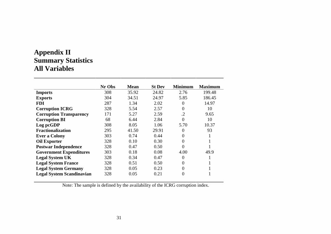
Appendix IISummary StatisticsAll Variables

Nr Obs Mean St Dev Minimum MaximumImports 308 35.92 24.82 2.76 199.48Exports 304 34.51 24.97 5.85 186.45FDI 287 1.34 2.02 0 14.97Corruption ICRG 328 5.54 2.57 0 10Corruption Transparency 171 5.27 2.59 .2 9.65Corruption BI 68 6.44 2.84 0 10Log pcGDP 308 8.05 1.06 5.70 10.37Fractionalization 295 41.50 29.91 0 93Ever a Colony 303 0.74 0.44 0 1Oil Exporter 328 0.10 0.30 0 1Postwar Independence 328 0.47 0.50 0 1Government Expenditures 303 0.18 0.08 4.00 49.9Legal System UK 328 0.34 0.47 0 1Legal System France 328 0.51 0.50 0 1Legal System Germany 328 0.05 0.23 0 1Legal System Scandinavian 328 0.05 0.21 0 1

Note: The sample is defined by the availability of the ICRG corruption index.

32

Appendix IIIInstrumenting for Openness

In this appendix we explain the procedure to develop new, more powerful, instruments forindicators of a country’s openness as measured by imports, exports and foreign direct investmentinflows. In the context of the present paper we wanted to find variables that were exogenous and didnot affect the degree of corruption directly. We have built four new variables that are likely to affectopenness but can at the same time be reasonably seen as totally exogenous to a country’s policychoices. The procedure was the following:

1. Select the 20 largest economies by Gross Domestic Product in 1990. The full list includesArgentina, Australia, Brazil, Canada, China, France, Germany, India, Indonesia, Iran, Italy, Japan,South Korea, Mexico, Netherlands, Poland, Spain, Turkey, the United Kingdom and the UnitedStates.

2. Compute, for each pair country in the sample – one of 20 largest economies, 4 variablesthat indicate the geographic and cultural closeness between each country in the sample and each ofthe 20 largest. The variables are: bilateral distance, dummy taking the value 1 if the country pair hasa common land border, dummy taking the value 1 if the country pair has the same majoritarianreligion and dummy taking the value 1 if the country pair shares an official language.

3. Take the constant US dollar value of exports, imports and foreign investment outflows ofeach of the 20 largest economies, averaged for each 5 year period, and multiply them by the dummyvariables constructed in 2. For bilateral distance, multiply the trade and investment flows by theinverse of the distance. The sum in each of the four categories (distance, contiguity, religion andlanguage) constitutes the instrument for the trade and investment openness of each country in thesample.

For example, each country in the sample will have four exogenous variables that will serveas instruments for its degree of trade openness, defined as:

TradeDI country i in the sample = SUM country j=1 to 20 of largest economies {( Inverse of

Bilateral Distance i,j ) * Exports j}TradeCO country i in the sample = SUM country j=1 to 20 of largest economies

{Contiguous i,j *

Exports j}TradeRE country i in the sample = SUM country j=1 to 20 of largest economies

{Religion i,j *

Exports j}TradeLA country i in the sample = SUM country j=1 to 20 of largest economies

{Language i,j *

Exports j}

The same four-fold of variables is built in a similar way for foreign investment outflows ofthe 20 largest economies. We are left with a group of exogenous variables that capture the export,import and trade impulses from the largest economies and weigh them by the geographical and

33

cultural proximity to each of the economies in the sample. These exogenous variables are thusdifferent for each of the openness indicators and, not least important, vary though time. This is asubstantial improvement relative to previous instruments for trade that were solely based onunchanging country characteristics.

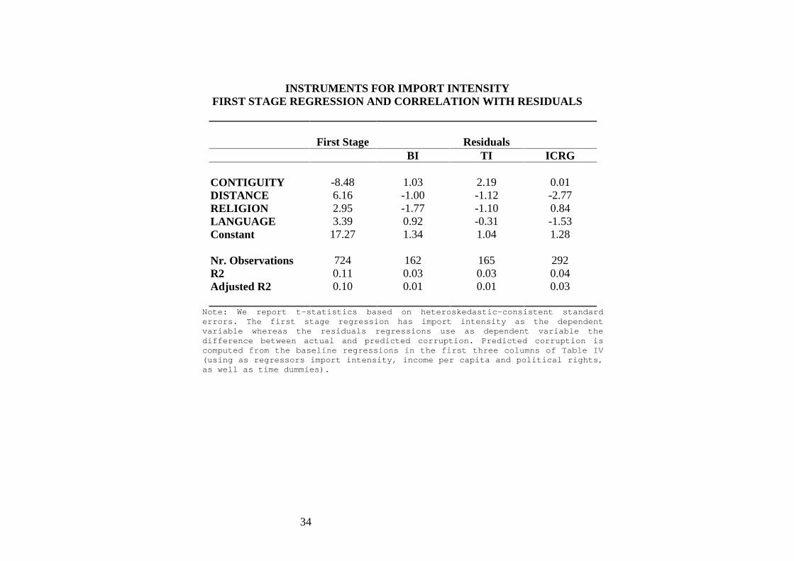
We regress actual imports, exports and FDI over GDP on the exogenous instruments listedabove. These first stage regressions have a strong predictive power, with R2 around 0.30. Thecorrelation between the exogenous and actual openness indicators range from 0.21 for FDI to 0.35and 0.38 for exports and imports, respectively. Thus, though the correlation is high, the variables arefar from displaying identical behavior. The coefficient on the exogenous determinants of opennessis significant and mostly come out with the expected sign. The predicted value of the dependentvariable in the regression above is then used in a second stage regression with a corruption index asthe dependent variable. We infer the causal effect of imports, exports and foreign direct investmenton a country’s level of corruption by examining the coefficient of openness in the second stageregression.

34

INSTRUMENTS FOR IMPORT INTENSITYFIRST STAGE REGRESSION AND CORRELATION WITH RESIDUALS

First Stage ResidualsBI TI ICRG

CONTIGUITY -8.48 1.03 2.19 0.01DISTANCE 6.16 -1.00 -1.12 -2.77RELIGION 2.95 -1.77 -1.10 0.84LANGUAGE 3.39 0.92 -0.31 -1.53Constant 17.27 1.34 1.04 1.28

Nr. Observations 724 162 165 292R2 0.11 0.03 0.03 0.04Adjusted R2 0.10 0.01 0.01 0.03

Note: We report t-statistics based on heteroskedastic-consistent standarderrors. The first stage regression has import intensity as the dependentvariable whereas the residuals regressions use as dependent variable thedifference between actual and predicted corruption. Predicted corruption iscomputed from the baseline regressions in the first three columns of Table IV(using as regressors import intensity, income per capita and political rights,as well as time dummies).