Stationary Analysis of a Fluid Queue Driven by Some Countable State Space Markov Chain
20
Methodol Comput Appl Probab (2007) 9:521–540 DOI 10.1007/s11009-006-9007-1 Stationary Analysis of a Fluid Queue Driven by Some Countable State Space Markov Chain Fabrice Guillemin · Bruno Sericola Received: 28 December 2005 / Revised: 11 September 2006 / Accepted: 19 September 2006 / Published online: 16 February 2007 © Springer Science + Business Media, LLC 2007 Abstract Motivated by queueing systems playing a key role in the performance evaluation of telecommunication networks, we analyze in this paper the station- ary behavior of a fluid queue, when the instantaneous input rate is driven by a continuous-time Markov chain with finite or infinite state space. In the case of an infinite state space and for particular classes of Markov chains with a countable state space, such as quasi birth and death processes or Markov chains of the G/M/1 type, we develop an algorithm to compute the stationary probability distribution function of the buffer level in the fluid queue. This algorithm relies on simple recurrence relations satisfied by key characteristics of an auxiliary queueing system with normalized input rates. Keywords fluid queues · Markov chains · uniformization · stationary regime · numerical algorithm AMS 2000 Subject Classification Primary 60K25 · Secondary 60J27 1 Introduction In the performance evaluation of packet telecommunication networks, fluid flow approximations prove very useful to analyze complex systems. Among fluid flow models, fluid queues with Markov modulated input rates play a key role in the recent developments of both queueing theory and performance evaluation of packet F. Guillemin France Telecom, 2 Avenue Pierre Marzin, 22300 Lannion, France e-mail: [email protected] B. Sericola (B ) IRISA-INRIA, Campus de Beaulieu, 35042 Rennes Cedex, France e-mail: [email protected]
-
Upload
independent -
Category
Documents
-
view
1 -
download
0
Transcript of Stationary Analysis of a Fluid Queue Driven by Some Countable State Space Markov Chain

Methodol Comput Appl Probab (2007) 9:521–540DOI 10.1007/s11009-006-9007-1
Stationary Analysis of a Fluid Queue Driven by SomeCountable State Space Markov Chain
Fabrice Guillemin · Bruno Sericola
Received: 28 December 2005 / Revised: 11 September 2006 /Accepted: 19 September 2006 / Published online: 16 February 2007© Springer Science + Business Media, LLC 2007
Abstract Motivated by queueing systems playing a key role in the performanceevaluation of telecommunication networks, we analyze in this paper the station-ary behavior of a fluid queue, when the instantaneous input rate is driven by acontinuous-time Markov chain with finite or infinite state space. In the case of aninfinite state space and for particular classes of Markov chains with a countablestate space, such as quasi birth and death processes or Markov chains of the G/M/1type, we develop an algorithm to compute the stationary probability distributionfunction of the buffer level in the fluid queue. This algorithm relies on simplerecurrence relations satisfied by key characteristics of an auxiliary queueing systemwith normalized input rates.
Keywords fluid queues · Markov chains · uniformization · stationary regime ·numerical algorithm
AMS 2000 Subject Classification Primary 60K25 · Secondary 60J27
1 Introduction
In the performance evaluation of packet telecommunication networks, fluid flowapproximations prove very useful to analyze complex systems. Among fluid flowmodels, fluid queues with Markov modulated input rates play a key role in therecent developments of both queueing theory and performance evaluation of packet
F. GuilleminFrance Telecom, 2 Avenue Pierre Marzin, 22300 Lannion, Francee-mail: [email protected]
B. Sericola (B)IRISA-INRIA, Campus de Beaulieu, 35042 Rennes Cedex, Francee-mail: [email protected]

522 Methodol Comput Appl Probab (2007) 9:521–540
networks (see for instance Boxma and Dumas, 1998). The first studies of suchqueueing systems can be dated back to the works by Kosten (1984) and Anick etal. (1982), who analyzed in the early 1980’s fluid models in connection with statisticalmultiplexing of several identical exponential on-off input sources in a buffer.
The above studies mainly focused on the analysis of the stationary regime andhave given rise to a series of theoretical developments. For instance, Mitra (1987)and (1988) generalizes this model by considering multiple types of exponential on–off inputs and outputs. Stern and Elwalid (1991) consider such models for separableMarkov modulated rate processes which lead to a solution of the equilibriumequations expressed as a sum of terms in Kronecker product form. Igelnik etal. (1995) derive a new approach, based on the use of interpolating polynomials,for the computation of the buffer overflow probability. Using the Wiener–Hopffactorization of finite Markov chains, Rogers (1994) shows that the distribution ofthe buffer level has a matrix exponential form, and Rogers and Shi (1994) explorealgorithmic issues of that factorization. Ramaswami (1996) and da Silva Soares andLatouche (2002) respectively exhibit and exploit the similarity between stationaryfluid queues in a finite Markovian environment and quasi birth and death processes.Ahn and Ramaswami (2003) establish a direct connection by stochastic couplingbetween fluid queues and quasi birth and death processes. Following the work ofSericola (1998) and that of Nabli and Sericola (1996), Nabli (2004) obtained analgorithm to compute the stationary distribution of a fluid queue driven by a finiteMarkov chain.
Most of the above cited studies have been carried out for finite modulatingMarkov chains. The analysis of a fluid queue driven by infinite state space Markovchains has also been addressed in many research papers. For instance, when thedriving process is the M/M/1 queue, Virtamo and Norros (1994) solve the associatedinfinite differential system by studying the continuous spectrum of a key matrix.Adan and Resing (1996) consider the background process as an alternating renewalprocess, corresponding to the successive idle and busy periods of the M/M/1 queue.By renewal theory arguments, the fluid level distribution is given in terms of integralof Bessel functions. They also obtain the expression of Virtamo and Norros via anintegral representation of Bessel functions. Barbot and Sericola (2002) obtain ananalytic expression for the joint stationary distribution of the buffer level and thestate of the M/M/1 queue. This expression is obtained by writing down the solutionin terms of a matrix exponential and then by using generating functions that areexplicitly inverted.
The Markov chain describing the number of customers in the M/M/1 queue isa specific birth and death process. Queueing systems with more general modulatinginfinite Markov chain have been studied by several authors. For instance, van Dornand Scheinhardt (1997) studied a fluid queue fed by an infinite general birth anddeath process using spectral theory. In Sericola and Tuffin (1999), the authorsconsider a fluid queue driven by a general Markovian queue with the hypothesisthat only one state has a negative drift. By using the differential system, the fluidlevel distribution is obtained in terms of a series, which coefficients are computedby means of recurrence relations. This study is extended to the finite buffer case inSericola (2001).
Besides the study of the stationary regime of fluid queues driven by finite orinfinite Markov chains, the transient analysis of such queues has been studied by

Methodol Comput Appl Probab (2007) 9:521–540 523
using Laplace transform by Kobayashi and Ren (1992) and Ren and Kobayashi(1995) for exponential on–off sources. These studies have been extended to theMarkov modulated input rate model by Tanaka et al. (1995). Sericola (1998) hasobtained a transient solution based on simple recurrence relations, which are particu-larly interesting for their numerical properties. More recently, Ahn and Ramaswami(2004) use an approach based on an approximation of the fluid model by the amountsof work in a sequence of Markov modulated queues of the quasi birth and death type.When the driving Markov chain has an infinite state space, the transient analysis ismore complicated. Sericola et al. (2005) consider the case of the M/M/1 queue byusing recurrence relations and Laplace transforms.
With respect to all above cited studies, the contribution of the present paperis to propose to a general algorithm for computing the stationary distribution andrelated characteristics of an infinite buffer fluid queue driven by a Markov chainwith a countable state space, while controlling the error made in the computations.The only assumption underlying the proposed algorithm is that some associatedMarkov chain can be uniformized. This means that the corresponding infinitesimalgenerator must have a finite norm. This restrictive assumption is needed becausethe solution we propose here is based on the uniformization technique (Ross, 1983).By using simple recurrence relations, we obtain in the case of infinite state spacesand for particular classes of countable Markov chains, such as quasi birth and deathprocesses or Markov chains of the G/M/1 type, algorithms to compute the stationarydistribution of the buffer level in the fluid queue. Clearly, the recurrence relationscan also be used to compute the stationary distribution of the buffer level in the fluidqueue, when the state space of the driving Markov chain is finite.
The paper is organized as follows. In Section 2, we present the model, the notationand the system of partial differential equations satisfied by the joint probabilitydistribution function of the buffer level and of the state of the driving process.Section 3 is devoted to the resolution of that system of partial differential equations;the solution is obtained in terms of a series. We first construct an equivalent fluidqueue with unit net input rates, which allows us to obtain simpler recurrence relationssatisfied by the coefficient of the series. In Section 4, we give details of somealgorithmic aspects of the buffer level distribution computation for general drivingprocesses and we give, in Section 5, the precise algorithms for particular classes ofdriving processes.
2 Model Description
We consider an infinite capacity fluid queue driven by a continuous-time Markovchain {Zt, t ≥ 0} on the countable state space S with infinitesimal generator A =(ai, j). The Markov chain {Zt} is supposed to be stationary and ergodic. We denote byβ j the output rate from state j given by β j = −a j, j and by π its stationary probabilitydistribution that satisfies π A = 0. The stationary distribution π has been studied inseveral papers for various special types of countable Markov chains such as birthand death processes, quasi birth and death processes or Markov chains of the G/M/1type. We refer the reader to Latouche and Ramaswami (1999), Meini (1998) and thereferences therein for the main results on this subject.
524 Methodol Comput Appl Probab (2007) 9:521–540
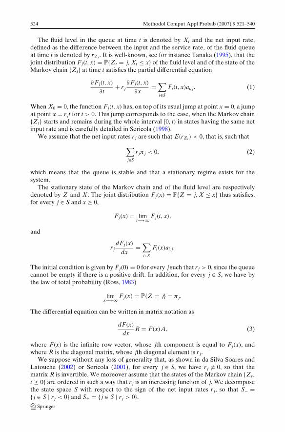
The fluid level in the queue at time t is denoted by Xt and the net input rate,defined as the difference between the input and the service rate, of the fluid queueat time t is denoted by rZt . It is well-known, see for instance Tanaka (1995), that thejoint distribution F j(t, x) = P{Zt = j, Xt ≤ x} of the fluid level and of the state of theMarkov chain {Zt} at time t satisfies the partial differential equation
∂ F j(t, x)
∂t+ r j
∂ F j(t, x)
∂x=
∑
i∈S
Fi(t, x)ai, j. (1)
When X0 = 0, the function F j(t, x) has, on top of its usual jump at point x = 0, a jumpat point x = r jt for t > 0. This jump corresponds to the case, when the Markov chain{Zt} starts and remains during the whole interval [0, t) in states having the same netinput rate and is carefully detailed in Sericola (1998).
We assume that the net input rates r j are such that E(rZt ) < 0, that is, such that
∑
j∈S
r jπ j < 0, (2)
which means that the queue is stable and that a stationary regime exists for thesystem.
The stationary state of the Markov chain and of the fluid level are respectivelydenoted by Z and X. The joint distribution F j(x) = P{Z = j, X ≤ x} thus satisfies,for every j ∈ S and x ≥ 0,
F j(x) = limt−→∞ F j(t, x),
and
r jdF j(x)
dx=
∑
i∈S
Fi(x)ai, j.
The initial condition is given by F j(0) = 0 for every j such that r j > 0, since the queuecannot be empty if there is a positive drift. In addition, for every j ∈ S, we have bythe law of total probability (Ross, 1983)
limx−→∞ F j(x) = P{Z = j} = π j.
The differential equation can be written in matrix notation as
dF(x)
dxR = F(x)A, (3)
where F(x) is the infinite row vector, whose jth component is equal to F j(x), andwhere R is the diagonal matrix, whose jth diagonal element is r j.
We suppose without any loss of generality that, as shown in da Silva Soares andLatouche (2002) or Sericola (2001), for every j ∈ S, we have r j �= 0, so that thematrix R is invertible. We moreover assume that the states of the Markov chain {Zt,
t ≥ 0} are ordered in such a way that r j is an increasing function of j. We decomposethe state space S with respect to the sign of the net input rates r j, so that S− ={ j ∈ S | r j < 0} and S+ = { j ∈ S | r j > 0}.

Methodol Comput Appl Probab (2007) 9:521–540 525
In the following, we denote by |M| the matrix obtained from matrix M by takingthe absolute values of its entries.
3 Solution to the Basic Matrix Equation
3.1 Notation and Preliminary Results
In this paper, we are interested in computing the quantity P(X > x) for x ≥ 0 andin designing an algorithm for obtaining the numerical value of this quantity with apredetermined round-off error ε. It turns out that instead of considering the originalsystem, it is more convenient in the computations to introduce an auxiliary system.It is easy to check that the matrix T = |R|−1 A is an infinitesimal generator. Define
λ = sup{β j/|r j| ; j ∈ S} (4)
and
r = inf{|r j| ; j ∈ S}. (5)
In the following, we make the two following assumptions:
(H1) The Markov chain with generator T can be uniformized, i.e., λ < ∞.(H2) The infimum of the absolute values of the net input rates is positive, i.e., r > 0.
Let ξ the stationary probability distribution corresponding to the matrix T, thatis, the row vector such that ξT = 0 and ξ� = 1, where � is the infinite column vectorwith all entries equal to 1. It is easy to check that ξ = π |R|/(π |R|�) or equivalentlythat π = ξ |R|−1/(ξ |R|−1�).
We denote by � the diagonal matrix with entries equal to −1 for the states of S−and equal to 1 for the states of S+, that is
� =(−I− 0
0 I+
),
where I− and I+ are the identity matrices corresponding to the subsets S− and S+,respectively.
As suggested in da Silva Soares and Latouche (2002), we rewrite Eq. (3) as
dF(x)
dx|R|� = F(x)|R|T. (6)
This amounts to introducing an auxiliary fluid queue with net input rates given by thematrix � and driven by the Markov chain with infinitesimal generator T. This latterqueue is stable and we denote by X and Z the stationary level in this queue and thestationary state of the driving Markov chain, respectively. The row vector G(x) ofthe joint distributions G j(x) = P{Z = j, X ≤ x} satisfies
dG(x)
dx� = G(x)T with G j(0) = 0 for j ∈ S+ and lim
x−→∞ G(x) = ξ.

526 Methodol Comput Appl Probab (2007) 9:521–540
We thus have
F(x) = G(x)|R|−1
ξ |R|−1�or equivalently G(x) = F(x)|R|
π |R|� .
The transient distribution of the couple (Z t, Xt) is denoted by the row vectorG(t, x), the jth component of this vector is G j(t, x) = P{Z t = j, Xt ≤ x}. Similarly toEq. (1), this transient distribution satisfies the following partial differential equation
∂G(t, x)
∂t+ ∂G(t, x)
∂x� = G(t, x)T. (7)
By taking as initial conditions X0 = 0 and P{Z 0 = j} = ξ j, for every j ∈ S, it is shownin Sericola (1998) that for every t > 0 and x ∈ [0, t), we have
G(t, x) =∞∑
n=0
e−λt (λt)n
n!n∑
k=0
(nk
) ( xt
)k (1 − x
t
)n−kb(n, k), (8)
where the infinite row vector b(n, k) = (bj(n, k), j ∈ S) is defined as follows. Forj ∈ S−,
bj(n, n) = ξ j for n ≥ 0, (9)
bj(n, k) = 1
2bj(n, k + 1) + 1
2
∑
i∈S
bi(n − 1, k)pi, j for k = n − 1, . . . , 0. (10)
and for j ∈ S+
bj(n, 0) = 0 for n ≥ 0, (11)
bj(n, k) =∑
i∈S
bi(n − 1, k − 1)pi, j for k = 1, . . . , n. (12)
where P = (pi, j) is the transition probability matrix of the uniformized Markov chainwith generator T with respect to the rate λ. This matrix is related to T by the relationP = I + T/λ, where I is the identity matrix with dimension given by the context andλ is defined by Eq. (4). The stationary probability distribution ξ satisfies ξ P = ξ .
In the next section, we show how to use the auxiliary queueing system withnet input rates given by matrix � and driven by the Markov chain with infinitesimalgenerator T to compute the probability distribution function (PDF) of the buffer X.
3.2 Computation of the Stationary PDF of the Buffer Level
By using the auxiliary queue with net input rates given by matrix � and driven by theMarkov chain with infinitesimal generator T, we have the following representationfor the complementary probability distribution function P(X > x).

Methodol Comput Appl Probab (2007) 9:521–540 527
Proposition 1 For fixed k ≥ 0, the sequence (b(n, k), n ≥ k) converges to a limit b(k)
as n → ∞ and the complementary probability distribution function of the stationarybuffer content X is given for fixed N by
P{X > x} =N∑
k=0
e−λx (λx)k
k! (1 − b(N, k)�) + e(x; N), (13)
where
e(x; N) =N∑
k=0
e−λx (λx)k
k! (b(N, k) − b(k))� +∞∑
k=N+1
e−λx (λx)k
k! (1 − b(k)�) (14)
and the column vector � is given by
� = |R|−1�
ξ |R|−1�= (π |R|�)|R|−1
�. (15)
To prove Proposition 1, we first establish a technical lemma describing theproperties of the sequence of vectors b(n, k). For the sake of simplicity, an inequalitybetween vectors of the same dimension means that the inequality stands for each oftheir entry (i.e., the inequality holds component by component).
Lemma 1 The row vectors b(n, k), n ≥ 0 and 0 ≤ k ≤ n, satisfy:
(a) For n ≥ 0 and 1 ≤ k ≤ n, 0 ≤ b(n, k − 1) ≤ b(n, k) ≤ ξ .(b) For n ≥ 1 and 1 ≤ k ≤ n, b(n − 1, k − 1) ≤ b(n, k).(c) For n ≥ 1 and 0 ≤ k ≤ n − 1, b(n, k) ≤ b(n − 1, k).(d) For n ≥ 1 and 0 ≤ k ≤ n − 2, b(n, k) ≤ b(n − 1, k + 1).
Proof Inequality (a) has been proven in Sericola (1998), in which we consider thevectors ξ − b(n, k) instead of the b(n, k). Inequality (d) follows from (c) and (a) bywriting b(n, k) ≤ b(n − 1, k) ≤ b(n − 1, k + 1). Inequalities (b) and (c) are proven inthe Appendix. �
We now proceed to the proof of Proposition 1.
Proof of Proposition 1 From Lemma 1, we deduce that for fixed k, the sequence(b(n, k), n ≥ k) is non increasing and non negative, and then converges as n goesto infinity. We denote by b(k) = (bj(k), j ∈ S) the limit of b(n, k) when n tends toinfinity. In other words, for j ∈ S, we have
limn−→∞ bj(n, k) = bj(k).
528 Methodol Comput Appl Probab (2007) 9:521–540
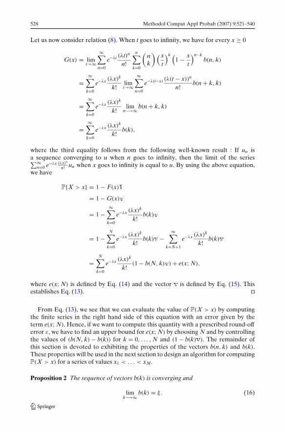
Let us now consider relation (8). When t goes to infinity, we have for every x ≥ 0
G(x) = limt→∞
∞∑
n=0
e−λt (λt)n
n!n∑
k=0
(nk
)( xt
)k (1 − x
t
)n−kb(n, k)
=∞∑
k=0
e−λx (λx)k
k! limt→∞
∞∑
n=0
e−λ(t−x) (λ(t − x))n
n! b(n + k, k)
=∞∑
k=0
e−λx (λx)k
k! limn−→∞ b(n + k, k)
=∞∑
k=0
e−λx (λx)k
k! b(k),
where the third equality follows from the following well-known result : If un isa sequence converging to u when n goes to infinity, then the limit of the series∑∞
n=0 e−λx (λx)n
n! un when x goes to infinity is equal to u. By using the above equation,we have
P{X > x} = 1 − F(x)�
= 1 − G(x)�
= 1 −∞∑
k=0
e−λx (λx)k
k! b(k)�
= 1 −N∑
k=0
e−λx (λx)k
k! b(k)� −∞∑
k=N+1
e−λx (λx)k
k! b(k)�
=N∑
k=0
e−λx (λx)k
k! (1 − b(N, k)�) + e(x; N),
where e(x; N) is defined by Eq. (14) and the vector � is defined by Eq. (15). Thisestablishes Eq. (13). �
From Eq. (13), we see that we can evaluate the value of P(X > x) by computingthe finite series in the right hand side of this equation with an error given by theterm e(x; N). Hence, if we want to compute this quantity with a prescribed round-offerror ε, we have to find an upper bound for e(x; N) by choosing N and by controllingthe values of (b(N, k) − b(k)) for k = 0, . . . , N and (1 − b(k)�). The remainder ofthis section is devoted to exhibiting the properties of the vectors b(n, k) and b(k).These properties will be used in the next section to design an algorithm for computingP(X > x) for a series of values x1 < . . . < xM.
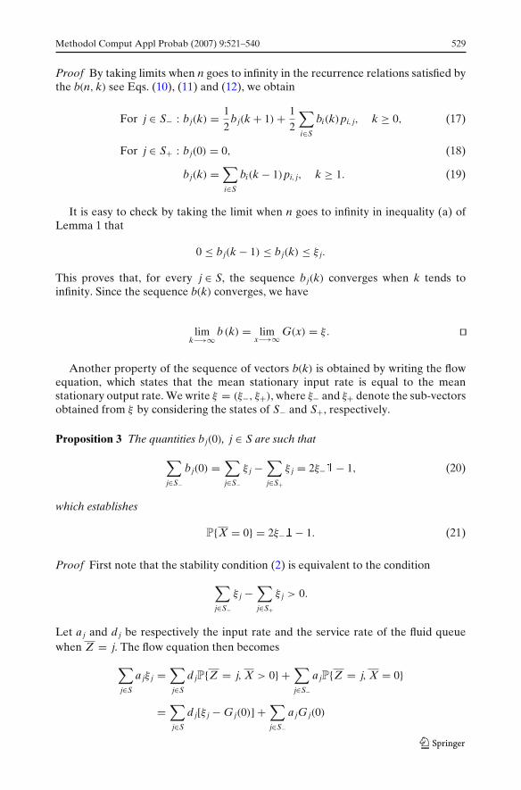
Proposition 2 The sequence of vectors b(k) is converging and
limk−→∞
b(k) = ξ. (16)
Methodol Comput Appl Probab (2007) 9:521–540 529
Proof By taking limits when n goes to infinity in the recurrence relations satisfied bythe b(n, k) see Eqs. (10), (11) and (12), we obtain
For j ∈ S− : bj(k) = 1
2bj(k + 1) + 1
2
∑
i∈S
bi(k)pi, j, k ≥ 0, (17)
For j ∈ S+ : bj(0) = 0, (18)
bj(k) =∑
i∈S
bi(k − 1)pi, j, k ≥ 1. (19)
It is easy to check by taking the limit when n goes to infinity in inequality (a) ofLemma 1 that
0 ≤ bj(k − 1) ≤ bj(k) ≤ ξ j.
This proves that, for every j ∈ S, the sequence bj(k) converges when k tends toinfinity. Since the sequence b(k) converges, we have
limk−→∞
b(k) = limx−→∞ G(x) = ξ. �
Another property of the sequence of vectors b(k) is obtained by writing the flowequation, which states that the mean stationary input rate is equal to the meanstationary output rate. We write ξ = (ξ−, ξ+), where ξ− and ξ+ denote the sub-vectorsobtained from ξ by considering the states of S− and S+, respectively.
Proposition 3 The quantities bj(0), j ∈ S are such that
∑
j∈S−
bj(0) =∑
j∈S−
ξ j −∑
j∈S+
ξ j = 2ξ−�− 1, (20)
which establishes
P{X = 0} = 2ξ−�− 1. (21)
Proof First note that the stability condition (2) is equivalent to the condition
∑
j∈S−
ξ j −∑
j∈S+
ξ j > 0.
Let a j and d j be respectively the input rate and the service rate of the fluid queuewhen Z = j. The flow equation then becomes
∑
j∈S
a jξ j =∑
j∈S
d jP{Z = j, X > 0} +∑
j∈S−
a jP{Z = j, X = 0}
=∑
j∈S
d j[ξ j − G j(0)] +∑
j∈S−
a jG j(0)

530 Methodol Comput Appl Probab (2007) 9:521–540
=∑
j∈S
d jξ j −∑
j∈S−
d jG j(0) +∑
j∈S−
a jG j(0)
=∑
j∈S
d jξ j +∑
j∈S−
(a j − d j)G j(0),
which can be written as∑
j∈S
(a j − d j)ξ j =∑
j∈S−
(a j − d j)G j(0).
Since for every j ∈ S, G j(0) = bj(0), and for j ∈ S−, we have a j − d j = −1, and forj ∈ S+, we have a j − d j = 1, we obtain the first equality of Eq. (20). The second oneis trivial by using the normalizing condition ξ+�+ ξ−� = 1. To get relation (21) wesimply write
P{X = 0} =∑
j∈S
G j(0) =∑
j∈S−
G j(0) =∑
j∈S−
bj(0),
and then we use relation (20). �
By using the above proposition and relations (17), (18) and (19), it can be easilyshown that for every k ≥ 0, we have
∑
j∈S−
bj(k) −∑
j∈S+bj(k) = 2ξ−�− 1.
As we did for ξ , we write b(n, k) = (b−(n, k), b+(n, k)) and b(k) = (b−(k), b+(k))
where b−(n, k), b+(n, k), b−(k) and b+(k) are the sub-vectors restricted to the statesof S− and S+, respectively.
Proposition 4 The vectors b(n, k) satisfy the inequalities
b(n − 1, k)�− b(n, k)� ≤ b−(n, 0)�− 2ξ−�+ 1, for n ≥ 1 and 0 ≤ k ≤ n − 1
(22)
and
ξ−�− b−(n, 0)� ≤ b+(n, n)� ≤ ξ+�, for n ≥ 0. (23)
Proof By summation over j in relation (10) at point (n, k − 1) and in relation (12) atpoint (n, k), we obtain
2∑
j∈S−
bj(n, k − 1) =∑
j∈S−
bj(n, k) +∑
i∈S
bi(n − 1, k − 1)∑
j∈S−
pi, j,
and∑
j∈S+
bj(n, k) =∑
i∈S
b i(n − 1, k − 1)∑
j∈S+
pi, j.

Methodol Comput Appl Probab (2007) 9:521–540 531
By adding these two relations, we obtain
2∑
j∈S−
bj(n, k − 1) +∑
j∈S+
bj(n, k) =∑
j∈S−
bj(n, k) +∑
j∈S
bj(n − 1, k − 1),
which can be written as
b−(n, k)�−b+(n, k)�=b−(n, k−1)�−b+(n, k−1)�+b(n, k−1)�−b(n−1, k−1)�.
Defining dn,k = b−(n, k)�− b+(n, k)�, we obtain
b(n − 1, k)�− b(n, k)� = dn,k − dn,k+1.
This quantity is positive from inequality (c) of Lemma 1. Hence, the sequence dn,k isdecreasing with respect to integer k. We then have, from inequality (a) of Lemma 1,
0 ≤ b(n − 1, k)�− b(n, k)� = dn,k − dn,k+1
≤ dn,0 − dn,n = b−(n, 0)�− ξ−�+ b+(n, n)�
≤ b−(n, 0)�− ξ−�+ ξ+� = b−(n, 0)�− 2ξ−�+ 1,
which completes the proof of relation (22).The right hand side of inequality (23) is the right hand side of inequality (a)
of Lemma 1. In order to prove the first inequality of Eq. 23, we use the fact thatthe sequence dn,k is decreasing with respect to integer k by writing that dn,n ≤ dn,0,that is
ξ−�− b+(n, n)� ≤ b−(n, 0)�,
which is the desired inequality. �
Propositions 3 and 4 are used in the next section in order to devise a numericalalgorithm for computing the quantity P(X > x) for different values x1 < . . . < xm.
4 Algorithmic Aspects
From Proposition 1, we see that we can compute P{X > x} with a prescribedprecision ε by using the series in the right hand side of Eq. (13) as soon as we canguarantee that the term e(x; N) defined by Eq. (14) is less than ε. This requiresto adequately choose N and to control the terms (b(N, k) − b(k)) and (1 − b(k)�).For this purpose, we first need to compute the vectors b(k). However, this taskis quite intricate because these vectors appear as limits of sequences of vectors(b(n, k), n ≥ k) defined by recurrence relations. By assuming that these sequencesare sufficiently smooth (typically that there is no step decrease), we approximateb(k) by b(n, k) as soon as b(n, k) − b(n + 1, k) ≤ ε, which means that the sequence(b(n, k)) is numerically stable and close to the limit b(k).

532 Methodol Comput Appl Probab (2007) 9:521–540
Denote by v the maximal entry of vector �. We have
v = sup{� j ; j ∈ S} = sup{1/|r j| ; j ∈ S}ξ |R|−1�
= 1
rξ |R|−1�= π |R|�
r,
where r is defined Eq. (5).We then define the integer N as the smallest integer n such that v(b−(n, 0) −
b−(0))� ≤ ε. From Proposition 3, we have b−(0)� = 2ξ−�− 1, so that N isdefined as
N = inf{n ≥ 0 | v(b−(n, 0)�− 2ξ−�+ 1) ≤ ε}. (24)
With this choice for N, we subsequently show that we have (b(N, k) −b(N + 1, k)) ≤ ε and (1 − b(N, k)�) ≤ ε so that we can expect that
(1 − b(k)�) ≤ ε and (b(N, k) − b(k)) ≤ ε,
which in turn implies that e(x; N) ≤ ε for all x ∈ R.For k = 0, we have, by definition of N and v,
(b(N, 0) − b(0))� ≤ v(b(N, 0) − b(0))� ≤ ε.
For k = 1, . . . , N, we have from Proposition 4 and by definition of N
(b(N, k) − b(N + 1, k))� ≤ v(b(N, k) − b(N + 1, k))�
≤ v(b(N + 1, 0)�− 2ξ−�+ 1)
≤ v(b(N, 0)�− 2ξ−�+ 1)
≤ ε,
so we expect that (b(N, k) − b(k))� ≤ ε.For k ≥ N + 1, from inequality (23) and since b−(n, n) = ξ−, we get
2ξ−�− b−(n, 0)� ≤ b(n, n)� ≤ 1,
that is
0 ≤ v(1 − b(n, n)�) ≤ v(b−(n, 0)�− 2ξ−�+ 1).
By definition of N, we have for k ≥ N,
0 ≤ v(1 − b(k, k)�) ≤ ε,
and we obtain for k ≥ N
1 − b(k, k)� = (ξ − b(k, k))� ≤ v(ξ − b(k, k))� = v(1 − b−(k, k)�) ≤ ε.
That is why we expect that (1 − b(k)�) ≤ ε, for k ≥ N.

Methodol Comput Appl Probab (2007) 9:521–540 533
Table 1 Algorithm for the computation of P{X > x}.input : x1 < · · · < xM, ε
output : P{X > x} for x = x1, . . . , xM
λ = sup{β j/|r j| ; j ∈ S}T = |R|−1 A
Compute the stationary distribution ξ
Compute the column vector � and v = sup{� j ; j ∈ S}P = I + T/λ
b+(0, 0) = 0
b−(0, 0) = ξ−n = 0
while v(b−(n, 0)�− 2ξ−�+ 1) > ε don = n+1
b+(n, 0) = 0
for k = 1 to n do compute b+(n, k) from Eq. (12) endforb−(n, n) = ξ−for k = n − 1 downto 0 do compute b−(n, k) from Eq. (10) endfor
endwhileN = n
for m = 1 to M do P{X > xm} =N∑
k=0
e−λxm(λxm)k
k! (1 − b(N, k)�) endfor
The above considerations lead us to expect that e(x; N) ≤ ε. We tested thisapproximation by considering fluid queues fed Markov chains with only one negativeeffective input rate. For such queues we developed in Sericola and Tuffin (1999) anexact algorithm which gives for a prescribed precision ε the same results as thoseobtained with the method presented in this paper. This supports the assumptionmade above on the smoothness of the sequences of vectors (b(n, k), n ≥ k), k ≥ 0.
The algorithm to compute the distribution Pr{X > x} for the M values x1 <
x2 < · · · < xM of x is then given in Table 1.Of course, this algorithm can be applied for every finite Markov chain. For infinite
state space Markov chains, the computation of the stationary distribution ξ and of theinfinite row vectors b(n, k) can be obtained only for special structures of the drivingMarkov chain. We deal with these particular types of structures in the followingsection.
5 Special Cases
In this section, we give a few examples of Markov chains for which the algorithmdescribed in Section 4 can be used for estimating the probability distribution functionof the buffer content in the stationary regime of a fluid queue driven by a Markovchain with a countable state space.

534 Methodol Comput Appl Probab (2007) 9:521–540
5.1 Fluid Queues Fed by Quasi Birth and Death Processes
The fluid queue is driven by a stationary ergodic continuous-time quasi birthand death (QBD) process, non necessarily homogeneous, represented by the two-dimensional Markov chain {Zt} on the state space S given by
S = {(�, j) : � ∈ �, 1 ≤ j ≤ m�},
where the first component is called the level and the second one is called the phase.The infinitesimal generator A of the QBD process is a block-tridiagonal infinitematrix that can be written as
A =
⎛
⎜⎜⎜⎜⎜⎜⎜⎝
A0,0 A0,1 0A1,0 A1,1 A1,2 0
0 A2,1 A2,2 A2,3. . .
0 A3,2 A3,3. . .
. . .. . .
. . .
⎞
⎟⎟⎟⎟⎟⎟⎟⎠
,
where, for � ≥ 0, the matrices A�,� are square matrices of dimension m� and thesizes of the other sub-matrices are determined accordingly. The computation of thestationary distribution π (or ξ) of the QBD process has been studied in severalpapers for various types of QBD processes. We refer the reader to Latouche andRamaswami (1999) and the references therein for the main results on this subject.
As we did for matrix A, we write the matrix R and the vectors b(n, k) and ξ byusing blocks, that is
R = diag(R0, R1, · · · , R�, R�+1, · · · ),
where R� is the diagonal matrix containing the entries r(�, j) for j = 1, . . . , m�,
b(n, k) = (b 0(n, k), b 1(n, k), . . . , b�(n, k), . . .),
with, for � ≥ 0,
b�(n, k) = (b(�,1)(n, k), . . . , b(�,m�)(n, k)),
and
ξ = (ξ0, ξ1, . . . , ξ�, . . .),
with, for � ≥ 0,
ξ� = (ξ(�,1), . . . , ξ(�,m�)).

Methodol Comput Appl Probab (2007) 9:521–540 535
We assume that r(�, j) > 0 when � is greater than a fixed �0 > 0 and that r(�, j) < 0for 0 ≤ � ≤ �0. We thus have S− = {(�, j) ∈ S : � ≤ �0} and S+ = {(�, j) ∈ S : � > �0}.The transition probability matrix P = I + T/λ can then be written as
P =
⎛
⎜⎜⎜⎜⎜⎜⎜⎜⎜⎝
P0,0 P0,1 0
P1,0 P1,1 P1,2 0
0 P2,1 P2,2 P2,3. . .
0 P3,2 P3,3. . .
. . .. . .
. . .
⎞
⎟⎟⎟⎟⎟⎟⎟⎟⎟⎠
,
where
P�,�+1 = |R�|−1 A�,�+1/λ,
P�,� = I + |R�|−1 A�,�/λ,
P�,�−1 = |R�|−1 A�,�−1/λ.
The relations (9), (10), (11), (12) can be written for 0 ≤ � ≤ �0 as
b�(n, n) = ξ� for n ≥ 0 (25)
b�(n, k) = 1
2b�(n, k + 1) + 1
2
[b�−1(n − 1, k)P�−1,� + b�(n − 1, k)P�,� ]
+ 1
2b�+1(n − 1, k)P�+1,� for k = n − 1, . . . , 0 (26)
and for � ≥ �0 + 1 as
b�(n, 0) = 0 for n ≥ 0 (27)
b�(n, k) = b�−1(n − 1, k − 1)P�−1,� + b�(n − 1, k − 1)P�,�
+ b�+1(n − 1, k − 1)P�+1,� for k = 1, . . . , n, (28)
where we set b−1(n − 1, k)P−1,0 = 0. The computation of each b�(n, k) requires afinite number of operations but the number of such vectors is infinite. This difficultyis overcome by the following result.
Lemma 2 For n ≥ 0 and 0 ≤ k ≤ n, we have
b�(n, k) = 0 for � ≥ �0 + k + 1.
Proof We proceed by recurrence over index k. For k = 0, we have from relation (11),bj(n, 0) = 0 for j ∈ S+ which means that b�(n, 0) = 0 for � ≥ �0 + 1.
Suppose that for a fixed index k ≥ 1, we have b�(n, k − 1) = 0 for � ≥ �0 + k, forevery n ≥ k − 1. This means in particular that
b�−1(n − 1, k − 1) = 0 for � ≥ �0 + k + 1
b�(n − 1, k − 1) = 0 for � ≥ �0 + k
b�+1(n − 1, k − 1) = 0 for � ≥ �0 + k − 1.

536 Methodol Comput Appl Probab (2007) 9:521–540
Thus, we obtain, from relation (28), that b�(n, k) = 0 for � ≥ �0 + k + 1. �
The above result means also that we only need to compute relation (28) for� = �0 + 1 to � = �0 + k.
5.2 Fluid Queues Fed by G/M/1 Type Markov Chains
Markov chains of the G/M/1 type have an infinitesimal generator with the followingHessenberg structure
A =
⎛
⎜⎜⎜⎜⎜⎜⎜⎜⎜⎝
A0,0 A0,1 0 0 · · ·A1,0 A1,1 A1,2 0 · · ·A2,0 A2,1 A2,2 A2,3
. . .
A3,0 A3,1 A3,2 A3,3. . .
......
. . .. . .
. . .
⎞
⎟⎟⎟⎟⎟⎟⎟⎟⎟⎠
,
on the same state space S as that used for QBDs. The computation of the stationarydistribution of such Markov chains can be found for instance in Meini (1998).
The matrix P has clearly the same structure and thus the recurrence relations (9),(10), (11), (12) become for 0 ≤ � ≤ �0
b�(n, n) = ξ� for n ≥ 0, (29)
b�(n, k) = 1
2b�(n, k + 1)
+ 1
2
∞∑
h=max(0,�−1)
bh(n − 1, k)Ph,� for k = n − 1, . . . , 0, (30)
and for � ≥ �0 + 1
b�(n, 0) = 0 for n ≥ 0, (31)
b�(n, k) =∞∑
h=�−1
bh(n − 1, k − 1)Ph,� for k = 1, . . . , n. (32)
In this case, the computation of each b�(n, k) requires an infinite number of opera-tions and the number of such vectors is infinite. These difficulties are overcome byusing Lemma 2, which is still valid. The recurrence relations (29), (30), (31), (32) thusbecome for 0 ≤ � ≤ �0
b�(n, n) = ξ� for n ≥ 0, (33)
b�(n, k) = 1
2b �(n, k + 1)
+ 1
2
�0+k∑
h=max(0,�−1)
bh(n − 1, k)Ph,� for k = n − 1, . . . , 0, (34)

Methodol Comput Appl Probab (2007) 9:521–540 537
and for � ≥ �0 + 1
b�(n, 0) = 0 for n ≥ 0 (35)
b�(n, k) =�0+k−1∑
h=�−1
bh(n − 1, k − 1)Ph,� for k = 1, . . . , n. (36)
This means that we only need to compute relation (36) for � = �0 + 1 to � = �0 + k.
5.3 Non-skip-free G/M/1 Type Markov Chains
Clearly, our method also applies for more general driving processes such as Markovchains of the non-skip-free G/M/1 type. The corresponding infinitesimal generator isan H-Hessenberg matrix, that is a matrix of the following form.
A =
⎛
⎜⎜⎜⎜⎜⎜⎜⎜⎜⎝
A0,0 · · · A0,H−1 A0,H 0 0 · · ·A1,0 · · · A1,H−1 A1,H A1,H+1 0 · · ·A2,0 · · · A2,H−1 A2,H A2,H+1 A2,H+2
. . .
A3,0 · · · A3,H−1 A3,H A3,H+1 A3,H+2. . .
......
.... . .
. . .. . .
⎞
⎟⎟⎟⎟⎟⎟⎟⎟⎟⎠
.
Appendix
Proof of Lemma 1
In this Appendix, we prove inequalities (b) and (c) appearing in Lemma 1.
Proof of inequality (b) The proof is by mathematical induction on the index n. Weuse inequality (a) of Lemma 1, i.e. 0 ≤ b(n, k) ≤ ξ .
For n = 1, we have
bj(1, 1) ≥ 0 = bj(0, 0) for j ∈ S+bj(1, 1) = ξ j = bj(0, 0) for j ∈ S−.
Suppose that for a fixed index n ≥ 1, we have
b(n, k) ≥ b(n − 1, k − 1) for 1 ≤ k ≤ n. (37)
We must show that for 1 ≤ k ≤ n + 1, we have b(n + 1, k) ≥ b(n, k − 1).Let j ∈ S+. By using the recurrence hypothesis (37), we obtain
bj(n + 1, k) − bj(n, k − 1) =∑
i∈S
(bi(n, k − 1) − bi(n − 1, k − 2))pi, j ≥ 0.
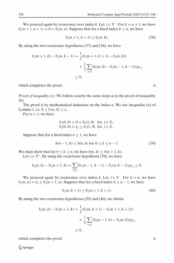
538 Methodol Comput Appl Probab (2007) 9:521–540
We proceed again by recurrence over index k. Let j ∈ S−. For k = n + 1, we havebj(n + 1, n + 1) = 0 = bj(n, n). Suppose that for a fixed index k ≤ n, we have
bj(n + 1, k + 1) ≥ bj(n, k). (38)
By using the two recurrence hypotheses (37) and (38), we have
bj(n + 1, k) − bj(n, k − 1) = 1
2(bj(n + 1, k + 1) − bj(n, k))
+ 1
2
∑
i∈S
(bj(n, k) − bj(n − 1, k − 1))pi, j
≥ 0,
which completes the proof. �
Proof of inequality (c) We follow exactly the same steps as in the proof of inequality(b).
The proof is by mathematical induction on the index n. We use inequality (a) ofLemma 1, i.e. 0 ≤ b(n, k) ≤ ξ .
For n = 1, we have
bj(0, 0) ≥ 0 = bj(1, 0) for j ∈ S+bj(0, 0) = ξ j ≥ bj(1, 0) for j ∈ S−.
Suppose that for a fixed index n ≥ 1, we have
b(n − 1, k) ≥ b(n, k) for 0 ≤ k ≤ n − 1. (39)
We must show that for 0 ≤ k ≤ n, we have b(n, k) ≥ b(n + 1, k).Let j ∈ S+. By using the recurrence hypothesis (39), we have
bj(n, k) − bj(n + 1, k) =∑
i∈S
(bi(n − 1, k − 1) − bi(n, k − 1))pi, j ≥ 0.
We proceed again by recurrence over index k. Let j ∈ S−. For k = n, we havebj(n, n) = ξ j ≥ bj(n + 1, n). Suppose that for a fixed index k ≤ n − 1, we have
bj(n, k + 1) ≥ bj(n + 1, k + 1). (40)
By using the two recurrence hypotheses (39) and (40), we obtain
bj(n, k) − bj(n + 1, k) = 1
2(bj(n, k + 1) − bj(n + 1, k + 1))
+ 1
2
∑
i∈S
(bj(n − 1, k) − bj(n, k))pi, j
≥ 0,
which completes the proof. �
Methodol Comput Appl Probab (2007) 9:521–540 539
References
I. Adan, and J. Resing, “Simple analysis of a fluid queue driven by an M/M/1 queue,” QueueingSystems—Theory and Applications vol. 22 pp. 171–174, 1996.
S. Ahn, and V. Ramaswami, “Fluid flow models and queues—a connection by stochastic coupling,”Communications in Statistics. Stochastic Models vol. 19(3) pp. 325–348, 2003.
S. Ahn, and V. Ramaswami, “Transient analysis of fluid flow models via stochastic coupling,”Communications in Statistics. Stochastic Models vol. 20(1) pp. 71–101, 2004.
D. Anick, D. Mitra, and M. M. Sondhi, “Stochastic theory of a data-handling system with multiplesources,” Bell System Technical Journal vol. 61(8) pp. 1871–1894, 1982.
N. Barbot, and B. Sericola, “Stationary solution to the fluid queue fed by an M/M/1 queue,” Journalof Applied Probability vol. 39 pp. 359–369, 2002.
O. J. Boxma, and V. Dumas, “The busy period in the fluid queue,” Performance Evaluation Reviewvol. 26 pp. 100–110, 1998.
A. da Silva Soares, and G. Latouche, “Further results on the similarity between fluid queues andQBDs.” In G. Latouche and P. Taylor (eds.), Proceedings of the 4th Int. Conf. on Matrix-AnalyticMethods, pp. 89–106, World Scientific: Adelaide, 2002.
B. Igelnik, Y. Kogan, V. Kriman, and D. Mitra, “A new computational approach for stochastic fluidmodels of multiplexers with heterogeneous sources,” Queueing Systems—Theory and Applica-tions vol. 20 pp. 85–116, 1995.
H. Kobayashi, and Q. Ren, “A mathematical theory for transient analysis of communicationnetworks,” IEICE Transactions on Communications vol.E75-B(12) pp. 1266–1276, 1992.
L. Kosten, “Stochastic theory of data-handling systems with groups of multiple sources.” In H. Rudinand W. Bux (eds.), Proceedings of the IFIP WG 7.3/TC 6 Second International Symposiumon the Performance of Computer–Communication Systems, Zurich, Switzerland, pp. 321–331,1984.
G. Latouche, and V Ramaswami, Introduction to Matrix Analytic Methods in Stochastic Modeling,In ASA-SIAM Series on Statistics and Applied Probability, SIAM, Philadelphia, PA, 1999.
B. Meini, “Solving M/G/1 type Markov chains : recent advances and applications,” Communicationsin Statistics. Stochastic Models vol. 14 pp. 479–496, 1998.
D. Mitra, “Stochastic fluid models.” In Proceedings of Performance’87, Brussels, Belgium, pp. 39–51,1987.
D. Mitra, “Stochastic theory of a fluid model of producers and consumers coupled by a buffer,”Advances in Applied Probability vol. 20 pp. 646–676, 1988.
H. Nabli, and B. Sericola, “Performability analysis: a new algorithm,” IEEE Transactions on Com-puters vol. 45 pp. 491–494, 1996.
H. Nabli, “Asymptotic solution of stochastic fluid models,” Performance evaluation vol. 57 pp. 121–140, 2004.
V. Ramaswami, “Matrix analytic methods for stochastic fluid flows.” In D. Smith and P. Hey (eds.),Proceedings ITC 16, pp. 1019–1030, Elsevier: Edinburgh, 1996.
Q. Ren, and H. Kobayashi, “Transient solutions for the buffer behavior in statistical multiplexing,”Performance evaluation vol. 23 pp. 65–87, 1995.
L. C. G. Rogers, and Z. Shi, “Computing the invariant law of a fluid model,” Journal of AppliedProbability vol. 31(4) pp. 885–896, 1994.
L. C. G. Rogers, “Fluid models in queueing theory and Wiener–Hopf factorization of Markovchains,” Annals of Applied Probability vol. 4(2) pp. 390–413, 1994.
S. M. Ross, Stochastic Processes, Wiley, New York, 1983.B. Sericola, P. R. Parthasarathy, and K. V. Vijayashree, “Exact transient solution of and M/M/1
driven fluid queue,” International Journal of Computer Mathematics vol. 82(6) pp. 659–671, 2005.B. Sericola, and B. Tuffin, “A fluid queue driven by a Markovian queue,” Queueing Systems—Theory
and Applications vol. 31 pp. 253–264, 1999.B. Sericola, “Transient analysis of stochastic fluid models,” Performance evaluation vol.32 pp. 245–
263, 1998.B. Sericola, “A finite buffer fluid queue driven by a Markovian queue,” Queueing Systems—Theory
and Applications vol. 38 pp. 213–220, 2001.T. E. Stern, and A. I. Elwalid, “Analysis of separable Markov-modulated rate models for
information-handling systems,” Advances in Applied Probability vol. 23 pp. 105–139, 1991.T. Tanaka, O. Hashida, and Y. Takahashi, “Transient analysis of fluid models for ATM statistical
multiplexer,” Performance evaluation vol. 23 pp. 145–162, 1995.

540 Methodol Comput Appl Probab (2007) 9:521–540
E. A. van Dorn, and W. R. Scheinhardt, “A fluid queue driven by an infinite-state birth and deathprocess.” In V. Ramaswami and P. Wirth (eds.), Proceedings ITC 15, pp. 465–475, Elsevier:Amsterdam, 1997.
J. Virtamo, and I. Norros, “Fluid queue driven by an M/M/1 queue,” Queueing Systems—Theory andApplications vol. 16 pp. 373–386, 1994.