An Obstacle-Free and Power-Efficient Deployment Algorithm for Wireless Sensor Networks

IEEE TRANSACTIONS ON SYSTEMS, MAN, AND CYBERNETICS—PART A: SYSTEMS AND HUMANS, VOL. 39, NO. 4, JULY 2009 795

An Obstacle-Free and Power-Efficient DeploymentAlgorithm for Wireless Sensor Networks

Chih-Yung Chang, Jang-Ping Sheu, Senior Member, IEEE, Yu-Chieh Chen, and Sheng-Wen Chang

Abstract—This paper proposes a robot-deployment algorithmthat overcomes unpredicted obstacles and employs full-coveragedeployment with a minimal number of sensor nodes. Withoutthe location information, node placement and spiral movementpolicies are proposed for the robot to deploy sensors efficiently toachieve power conservation and full coverage, while an obstaclesurrounding movement policy is proposed to reduce the impactsof an obstacle upon deployment. Simulation results reveal thatthe proposed robot-deployment algorithm outperforms most ex-isting robot-deployment mechanisms in power conservation andobstacle resistance and therefore achieves a better deploymentperformance.

Index Terms—Deployment, obstacle, placement, robot, wirelesssensor networks (WSNs).

I. INTRODUCTION

R ECENT advances in digital electronics, microprocessors,and wireless communication have made sensors smaller,

low powered, and cheaper to manufacture [1]. Due to theseattractive characteristics, wireless sensor networks (WSNs) arenow widely applied to many applications, which include envi-ronmental monitoring, tracking, precision agriculture, militarysurveillance, smart homes, and so on [2]–[7]. WSNs are large-scale distributed systems composed of a large number of sen-sors and a few sinks. Sensors are responsible for collecting thesensed information and sending them to sinks in a multihopmanner. A sink is the interface between the sensors and users,executing tasks that include accepting the user’s command,delivering the data request criteria to the sensors, collectingthe interested data from the sensors, and integrating them toprovide the user with advanced uses.

Developing a good deployment algorithm is one of the mostimportant issues for an efficient WSN. In the literature, existingdeployment algorithms can be classified into three categories:stationary sensor, mobile sensor, and mobile robot. Several

Manuscript received February 13, 2007; revised May 24, 2008. First pub-lished April 17, 2009; current version published June 19, 2009. This work wassupported in part by the National Science Council, Taiwan. This paper wasrecommended by Associate Editor A. Ollero.

C.-Y. Chang, Y.-C. Chen, and S.-W. Chang are with the Departmentof Computer Science and Information Engineering, Tamkang University,Tamsui 25137, Taiwan (e-mail: [email protected]; [email protected]; [email protected]).

J.-P. Sheu is with the Department of Computer Science and InformationEngineering, National Tsing Hua University, Hsinchu 30013, Taiwan (e-mail:[email protected]).

Color versions of one or more of the figures in this paper are available onlineat http://ieeexplore.ieee.org.

Digital Object Identifier 10.1109/TSMCA.2009.2014389

random deployment schemes [8], [9] have been proposed forthe deployment of stationary sensors. The random deploymentscheme is simple and easy to implement. However, to ensurefull coverage, its number of deployed sensors is extremelylarger than the actual required number of sensors. The randomdeployment of stationary sensors may result in an inefficientWSN wherein some areas have a high density of sensors whileothers have a low density. Areas with high density increasehardware costs, computation time, and communication over-heads, whereas areas with low density may raise the problemsof coverage holes or network partitions. Other works [10]–[13]have discussed deployment using mobile sensors. Mobile sen-sors first cooperatively compute for their target locations ac-cording to their information on holes after an initial phase ofrandom deployment of stationary sensors and then move to tar-get locations. However, hardware costs cannot be lessened forareas that have a high density of stationary sensors deployed.

Another deployment alternative [14]–[17] is to use the robotto deploy static sensors. The robot explores the environmentand deploys a stationary sensor to the target location fromtime to time. The robot deployment can achieve full coveragewith fewer sensors, increase the sensing effectiveness of sta-tionary sensors, and guarantee full coverage and connectivity.Aside from this, the robot may perform other missions suchas hole-detection, redeployment, and monitoring. However,unpredicted obstacles are a challenge of robot deployment andhave a great impact on deployment efficiency. One of the mostimportant issues in developing a robot-deployment mechanismis to use fewer sensors for achieving both full coverage andenergy-efficient purposes even if the monitoring region containsunpredicted obstacles.

Obstacles such as walls, buildings, blockhouses, and pill-boxes might exist in the outdoor environment. These obsta-cles significantly impact the performance of robot deployment.A robot-deployment algorithm without considering obstaclesmight result in coverage holes or might spend a long timeexecuting a deployment task. In the literature, Batalin andSukhatme [14] assume that the robot is equipped with a com-pass which makes it aware of its movement direction. A robotmovement strategy that uses deployed sensors to guide a robot’smovement as well as sensor deployment in a given area is pro-posed. Although the proposed robot-deployment scheme likelyachieves the purpose of full coverage and network connectivity,it does not, however, take into account the obstacles. The nextmovement of the robot is guided from only the nearest sensornode, raising problems of coverage holes or overlapping in thesensing range as the robot encounters obstacles. Aside fromthis, during robot deployment, all deployed sensors stay in an

1083-4427/$25.00 © 2009 IEEE

Authorized licensed use limited to: Tamkang University. Downloaded on July 12, 2009 at 08:52 from IEEE Xplore. Restrictions apply.

796 IEEE TRANSACTIONS ON SYSTEMS, MAN, AND CYBERNETICS—PART A: SYSTEMS AND HUMANS, VOL. 39, NO. 4, JULY 2009

active state in order to participate in guiding tasks, resulting inan inefficiency in power consumption.

To handle obstacle problems, a previous research [17] hasproposed a centralized algorithm that uses global obstacleinformation to calculate for the best deployment locationof each sensor. Although the proposed mechanism achievesfull coverage and connectivity using fewer stationary sensors,global obstacle information is required, which makes the de-veloped robot-deployment mechanism useful only in limitedapplications.

This work aims to develop an obstacle-free robot-deployment algorithm. Unpredicted obstacles are taken intoconsideration in the proposed mechanism so full coverage canbe likely achieved with the deployment of a minimal number ofsensors. Moreover, most deployed sensors may stay in a sleepstate to reduce power consumption during robot deployment.Simulation results show that the proposed algorithm signifi-cantly reduces the total number of deployed stationary sensors,achieves full coverage, and saves on energy consumption.

The rest of this paper is organized as follows. Section IIfirst reviews related work; then, the network model and thebasic concept of this paper are given. Section III gives thedetails of the robot-deployment algorithm. The node placementand spiral movement policies are proposed without consideringthe existence of obstacles. Section IV presents the obstaclehandling mechanism and discusses the energy conservationissue. The performance study is presented in Section V. Finally,conclusions are drawn in Section VI.

II. RELATED WORK AND BASIC CONCEPTS

This section initially describes related work on robot deploy-ment. Later on, the network environment and basic concepts ofthis paper are introduced with examples.

A. Related Work

Compared with random deployment, using the robot to step-wise deploy static sensors in a specific region can give fullsensing coverage with fewer sensors. Previous research [14]assumes that the robot is equipped with a compass and is ableto detect obstacles. Each sensor has a communication range rc

and a sensing range rs. To guide the robot’s movement, eachdeployed sensor maintains a time duration for each direction,whether south, east, north, or west, that the robot did not visit.The longer the time length, the higher priority the direction is.When the robot intends to make a movement decision, it com-municates with the closest deployed sensor, queries the timelength of each direction, and then selects one direction with thehighest priority to be the direction of its next movement.

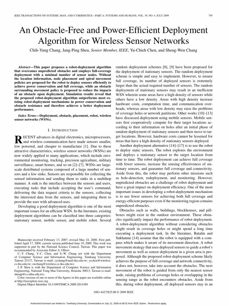
Although the robot-deployment algorithm developed in [14]likely achieves the purpose of full coverage and network con-nectivity, the next movement of the robot is guided by onlyone sensor, resulting in it taking a long time to achieve fullcoverage and requiring more sensors due to a big overlappingarea. As shown in Fig. 1(a), assume that sensors sk and sj werepreviously deployed in the monitoring area and sensor si isthe most recently deployed sensor. According to the guiding

Fig. 1. Drawback of the algorithm in [14] is due to the situation where thenext movement of the robot is guided by only one sensor. (a) Coverage hole.(b) Many overlapping areas. (c) Improved deployment.

of sensor si, the robot will move east and deploy sensor si+1,resulting in a hole this time even though sensor sk is in thecommunication range of the robot. A sensor will be deployedto the hole after a long period. Fig. 1(b) shows another example.Assume that the distance between si and sk is smaller than rs.The robot only guided by si may deploy a sensor si+1 to thelocation that overlaps a lot of the sensing regions of sk andsj , requiring more sensors to be deployed on the whole targetregion. This paper develops an efficient robot-deployment algo-rithm. The robot will be guided by si and sk at the same time toachieve full coverage and network connectivity purposes usingfewer deployed sensors. The improved deployment in this caseis shown in Fig. 1(c). The overlapping area among the sensingranges of si, si+1, and sk is minimal, achieving full coverageby using fewer sensors.

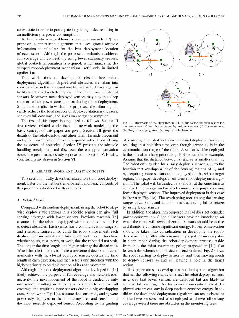
In addition, the algorithm proposed in [14] does not considerpower conservation. Since all sensors have no knowledge onwhen the robot will revisit them, all sensors should be activeand therefore consume significant energy. Power conservationshould be taken into consideration in developing the robot-deployment algorithm wherein most deployed sensors may stayin sleep mode during the robot-deployment process. Asidefrom this, the robot movement policy proposed in [14] alsoleaves holes whenever an obstacle is encountered. Fig. 2 showsthe robot starting to deploy sensor s1 and then moving southto deploy sensors s2 and s3, leaving a hole in the targetregion.

This paper aims to develop a robot-deployment algorithmthat has the following characteristics. The robot deploys sensorsin a way that fewer sensors are deployed but are likely toachieve full coverage. As for power conservation, most de-ployed sensors can stay in sleep mode to conserve energy. In ad-dition, the developed deployment algorithm can resist obstaclesso that fewer sensors need to be deployed to achieve full sensingcoverage even if there are obstacles in the monitoring area.


CHANG et al.: OBSTACLE-FREE AND POWER-EFFICIENT DEPLOYMENT ALGORITHM FOR WSNs 797

Fig. 2. Robot movement policy leaves a hole when an obstacle is encountered.

B. Network Environment and Protocol Overview

1) Network Environment: This paper assumes that the robotis aware of its own location information. This assumption canbe achieved if the robot is equipped with both GPS and compassmodules which provide the current location and moving direc-tion of the robot, respectively. Although the GPS localizationsystem might have an inaccuracy range, the other localizationsystem based on the compass module could help estimatethe current location of the robot according to the movementdirection provided by the compass as well as the distance,which can be calculated based on the rotation rate of the robot’swheels. We also assume that the monitoring field is a 2-D planewhere there may exist obstacles in the field and that the robot isembedded with a radio system that enables it to communicatewith deployed sensors in a wireless manner. Aside from this,the robot is also able to discover unknown obstacles as it movescloser to them. Let symbol sm denote a sensor, 0 ≤ m ≤ N ,where N is the number of sensors required for full coverage.The communication range is denoted by rc, while the sensingrange is denoted by rs, and they both satisfy the relationrc ≥ √

3rs. Given two locations p and q in the monitoringfield, symbol d(p, q) represents the distance of p and q. In thefollowing, an example is given to illustrate the basic idea of theproposed robot-deployment protocol.

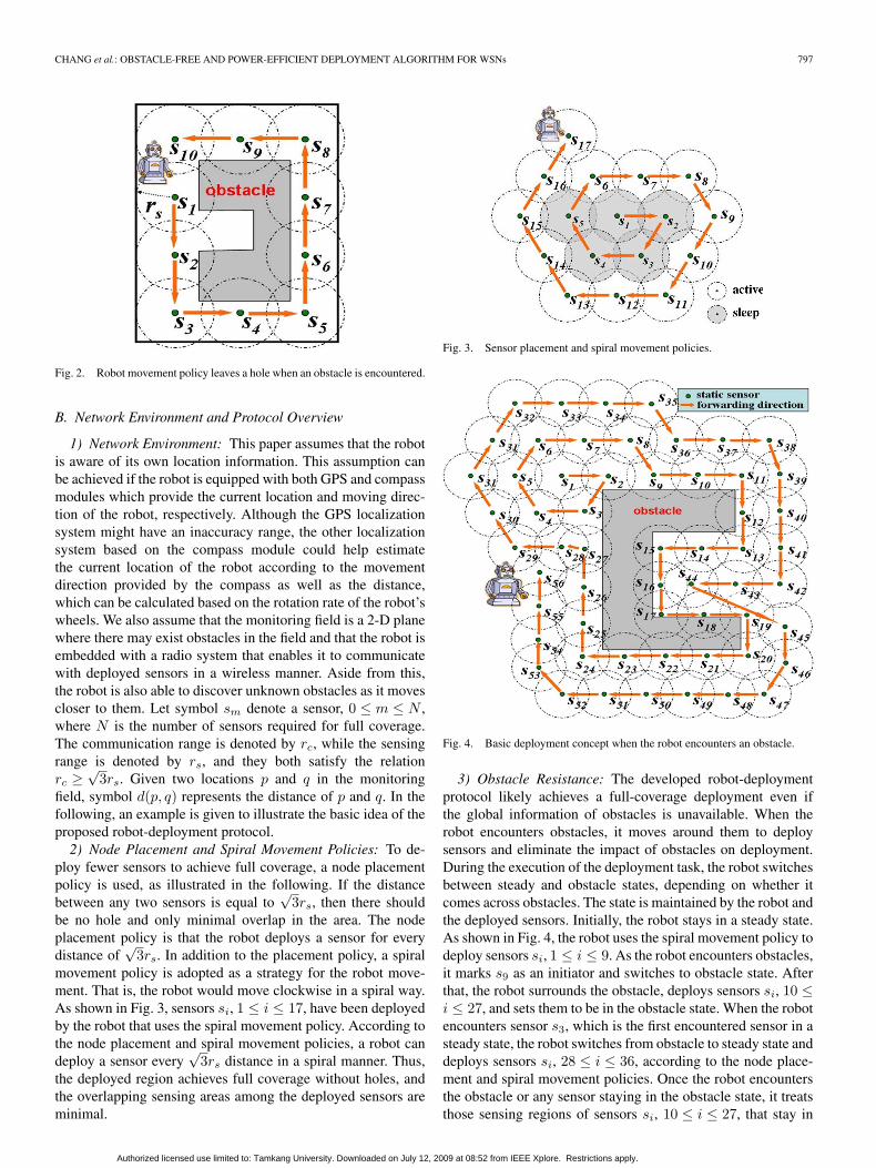
2) Node Placement and Spiral Movement Policies: To de-ploy fewer sensors to achieve full coverage, a node placementpolicy is used, as illustrated in the following. If the distancebetween any two sensors is equal to

√3rs, then there should

be no hole and only minimal overlap in the area. The nodeplacement policy is that the robot deploys a sensor for everydistance of

√3rs. In addition to the placement policy, a spiral

movement policy is adopted as a strategy for the robot move-ment. That is, the robot would move clockwise in a spiral way.As shown in Fig. 3, sensors si, 1 ≤ i ≤ 17, have been deployedby the robot that uses the spiral movement policy. According tothe node placement and spiral movement policies, a robot candeploy a sensor every

√3rs distance in a spiral manner. Thus,

the deployed region achieves full coverage without holes, andthe overlapping sensing areas among the deployed sensors areminimal.

Fig. 3. Sensor placement and spiral movement policies.

Fig. 4. Basic deployment concept when the robot encounters an obstacle.

3) Obstacle Resistance: The developed robot-deploymentprotocol likely achieves a full-coverage deployment even ifthe global information of obstacles is unavailable. When therobot encounters obstacles, it moves around them to deploysensors and eliminate the impact of obstacles on deployment.During the execution of the deployment task, the robot switchesbetween steady and obstacle states, depending on whether itcomes across obstacles. The state is maintained by the robot andthe deployed sensors. Initially, the robot stays in a steady state.As shown in Fig. 4, the robot uses the spiral movement policy todeploy sensors si, 1 ≤ i ≤ 9. As the robot encounters obstacles,it marks s9 as an initiator and switches to obstacle state. Afterthat, the robot surrounds the obstacle, deploys sensors si, 10 ≤i ≤ 27, and sets them to be in the obstacle state. When the robotencounters sensor s3, which is the first encountered sensor in asteady state, the robot switches from obstacle to steady state anddeploys sensors si, 28 ≤ i ≤ 36, according to the node place-ment and spiral movement policies. Once the robot encountersthe obstacle or any sensor staying in the obstacle state, it treatsthose sensing regions of sensors si, 10 ≤ i ≤ 27, that stay in



Fig. 5. Optimal deployment of sensors si, sj , and sk .

obstacle state as virtual obstacles and uses a similar way to over-come these obstacles. In the obstacle state, the robot maintainsthe locations of the deployed sensors in Stack. Whenever therobot moves to a location that is surrounded by the deployedsensors, it pops the location from Stack and moves to it untilthe robot is not surrounded by the deployed sensors. Fig. 4shows an example to illustrate how the robot copes with thedead-end problem. Let pos(s) denote the location of a deployedsensor s. When the robot deploys sensor s44, it subsequentlypops locations pos(s43) and pos(s42) from Stack and deploysa new sensor s45. Finally, the robot deploys sensors around theobstacle until the deployed sensors cover the entire monitor-ing area.

III. ROBOT-DEPLOYMENT ALGORITHM

This section describes the deployment algorithm thatachieves full coverage with fewer sensors. The algorithmmainly consists of a node placement policy and a spiral move-ment policy.

A. Node Placement Policy

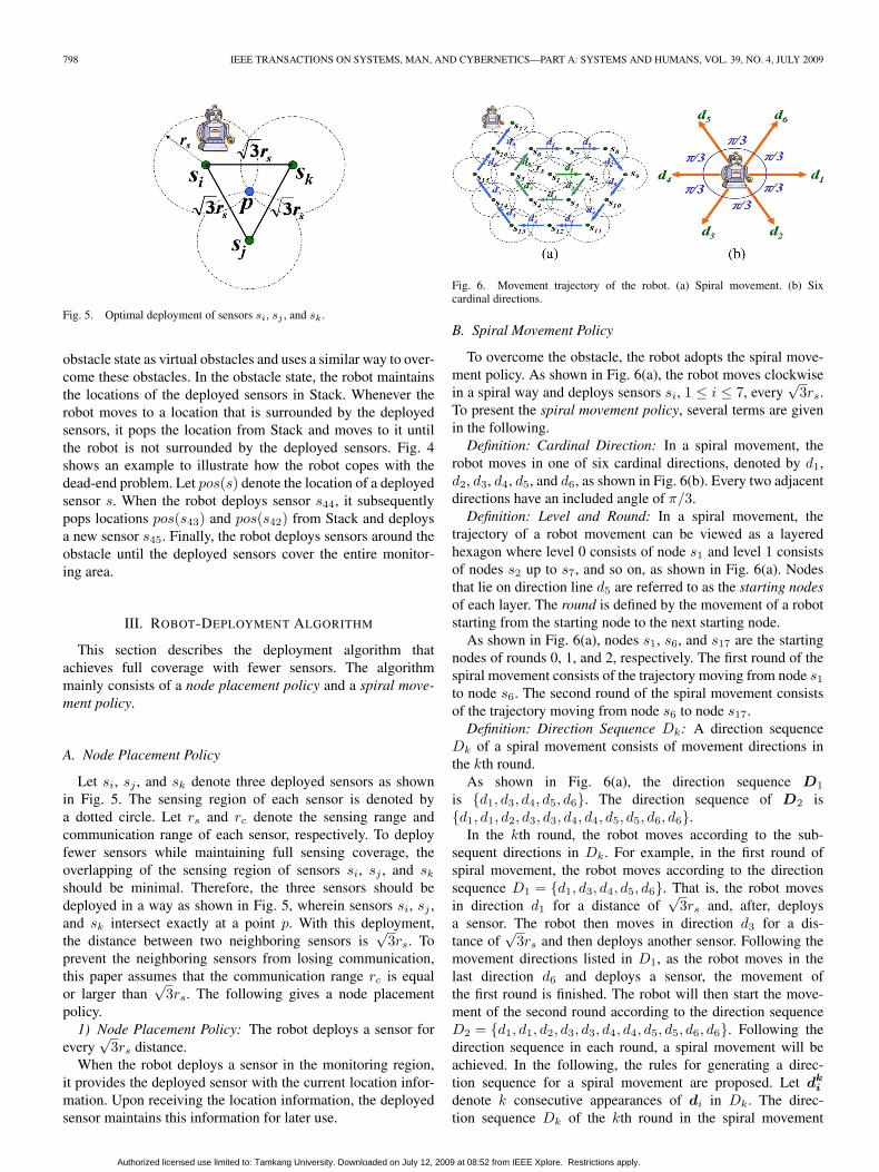
Let si, sj , and sk denote three deployed sensors as shownin Fig. 5. The sensing region of each sensor is denoted bya dotted circle. Let rs and rc denote the sensing range andcommunication range of each sensor, respectively. To deployfewer sensors while maintaining full sensing coverage, theoverlapping of the sensing region of sensors si, sj , and sk

should be minimal. Therefore, the three sensors should bedeployed in a way as shown in Fig. 5, wherein sensors si, sj ,and sk intersect exactly at a point p. With this deployment,the distance between two neighboring sensors is

√3rs. To

prevent the neighboring sensors from losing communication,this paper assumes that the communication range rc is equalor larger than

√3rs. The following gives a node placement

policy.1) Node Placement Policy: The robot deploys a sensor for

every√

3rs distance.When the robot deploys a sensor in the monitoring region,

it provides the deployed sensor with the current location infor-mation. Upon receiving the location information, the deployedsensor maintains this information for later use.

Fig. 6. Movement trajectory of the robot. (a) Spiral movement. (b) Sixcardinal directions.

B. Spiral Movement Policy

To overcome the obstacle, the robot adopts the spiral move-ment policy. As shown in Fig. 6(a), the robot moves clockwisein a spiral way and deploys sensors si, 1 ≤ i ≤ 7, every

√3rs.

To present the spiral movement policy, several terms are givenin the following.

Definition: Cardinal Direction: In a spiral movement, therobot moves in one of six cardinal directions, denoted by d1,d2, d3, d4, d5, and d6, as shown in Fig. 6(b). Every two adjacentdirections have an included angle of π/3.

Definition: Level and Round: In a spiral movement, thetrajectory of a robot movement can be viewed as a layeredhexagon where level 0 consists of node s1 and level 1 consistsof nodes s2 up to s7, and so on, as shown in Fig. 6(a). Nodesthat lie on direction line d5 are referred to as the starting nodesof each layer. The round is defined by the movement of a robotstarting from the starting node to the next starting node.

As shown in Fig. 6(a), nodes s1, s6, and s17 are the startingnodes of rounds 0, 1, and 2, respectively. The first round of thespiral movement consists of the trajectory moving from node s1

to node s6. The second round of the spiral movement consistsof the trajectory moving from node s6 to node s17.

Definition: Direction Sequence Dk: A direction sequenceDk of a spiral movement consists of movement directions inthe kth round.

As shown in Fig. 6(a), the direction sequence D1

is {d1, d3, d4, d5, d6}. The direction sequence of D2 is{d1, d1, d2, d3, d3, d4, d4, d5, d5, d6, d6}.

In the kth round, the robot moves according to the sub-sequent directions in Dk. For example, in the first round ofspiral movement, the robot moves according to the directionsequence D1 = {d1, d3, d4, d5, d6}. That is, the robot movesin direction d1 for a distance of

√3rs and, after, deploys

a sensor. The robot then moves in direction d3 for a dis-tance of

√3rs and then deploys another sensor. Following the

movement directions listed in D1, as the robot moves in thelast direction d6 and deploys a sensor, the movement ofthe first round is finished. The robot will then start the move-ment of the second round according to the direction sequenceD2 = {d1, d1, d2, d3, d3, d4, d4, d5, d5, d6, d6}. Following thedirection sequence in each round, a spiral movement will beachieved. In the following, the rules for generating a direc-tion sequence for a spiral movement are proposed. Let dk

i

denote k consecutive appearances of di in Dk. The direc-tion sequence Dk of the kth round in the spiral movement



can be automatically generated by the robot according to thefollowing:

Dk ={dk1 , dk−1

2 , dk3 , dk

4 , dk5 , dk

6

}, k ∈ Z+.

For example, the robot can generate the movement directionsequence Dk using

k = 1, D1 = {d1, d3, d4, d5, d6}k = 2, D2 = {d1, d1, d2, d3, d3, d4, d4, d5, d5, d6, d6}k = 3, D3 = {d1, d1, d1, d2, d2, d3, d3, d3, d4, d4, d4,

d5, d5, d5, d6, d6, d6} and so on.

Therefore, the robot will move according to the followingspiral movement policy.

Spiral Movement Policy: The robot moves a distance of√3rs in a specific direction according to the direction sequence

Dk in the kth round and then deploys a sensor, where

Dk ={dk1 , dk−1

2 , dk3 , dk

4 , dk5 , dk

6

}, k ∈ Z+.

IV. OBSTACLE HANDLING

This section introduces the obstacle handling mechanism thatovercomes unknown obstacles in order to achieve full-coveragedeployment. Two types of states are used to distinguish whetherthe robot encounters obstacles, namely, the steady and obstaclestates. In the steady state, the robot moves and deploys sensorsfollowing the aforementioned spiral movement and sensor de-ployment policies. When the robot encounters an obstacle, itswitches from steady to obstacle state and moves and deployssensors according to an obstacle surrounding movement policywhich is introduced in the following to reduce the negativeimpacts of an obstacle upon deployment.

A. Obstacle Surrounding Movement Policy

To reduce the impact of an obstacle upon deployment, theobstacle surrounding movement policy is employed in thissection. When the robot encounters obstacles, it switches fromsteady to obstacle state. In the obstacle state, the robot adoptsthe obstacle surrounding movement policy, in which the robotmoves clockwise around the obstacle and deploys sensors tohave full coverage. Some terms are introduced first to makethe illustration clear. The guiding sensor is the most recentlydeployed sensor. Note that the guiding sensor is closest to therobot. The reference sensor refers to the deployed sensor thatis second closest to the robot. It is observed that the distancesbetween any pair of three locations, including the expectedlocation, the location of the guiding sensor, and the locationof the reference sensor, are exactly

√3rs apart. Let the initiator

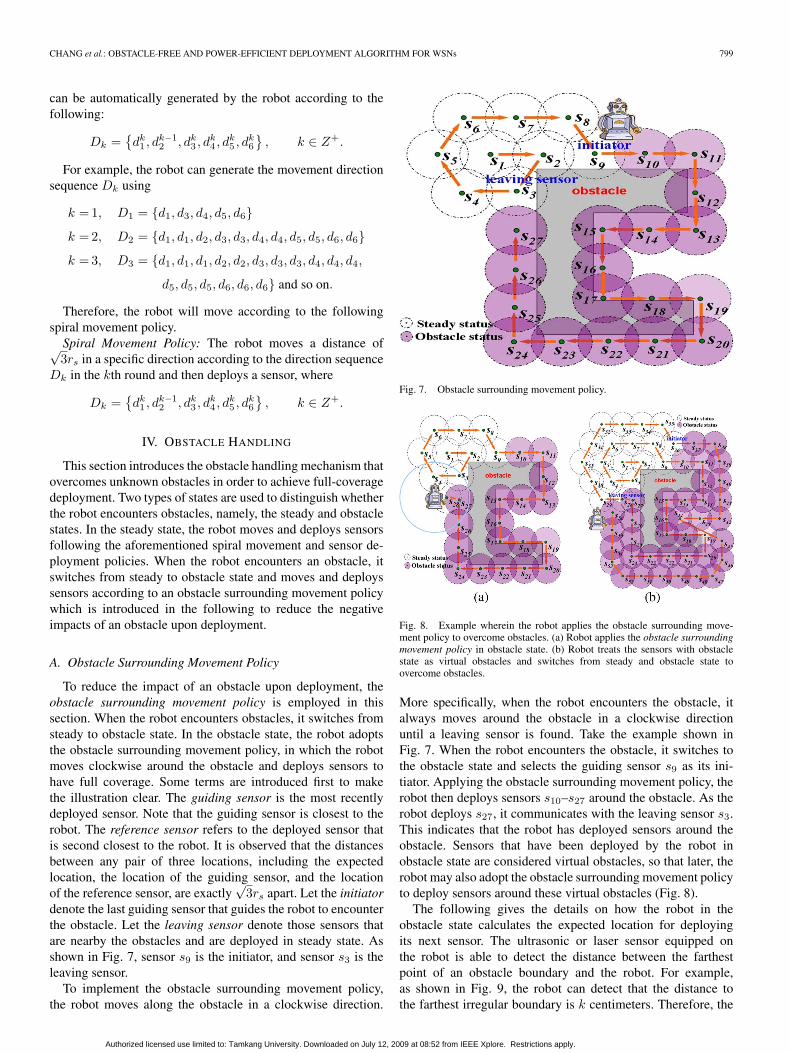
denote the last guiding sensor that guides the robot to encounterthe obstacle. Let the leaving sensor denote those sensors thatare nearby the obstacles and are deployed in steady state. Asshown in Fig. 7, sensor s9 is the initiator, and sensor s3 is theleaving sensor.

To implement the obstacle surrounding movement policy,the robot moves along the obstacle in a clockwise direction.

Fig. 7. Obstacle surrounding movement policy.

Fig. 8. Example wherein the robot applies the obstacle surrounding move-ment policy to overcome obstacles. (a) Robot applies the obstacle surroundingmovement policy in obstacle state. (b) Robot treats the sensors with obstaclestate as virtual obstacles and switches from steady and obstacle state toovercome obstacles.

More specifically, when the robot encounters the obstacle, italways moves around the obstacle in a clockwise directionuntil a leaving sensor is found. Take the example shown inFig. 7. When the robot encounters the obstacle, it switches tothe obstacle state and selects the guiding sensor s9 as its ini-tiator. Applying the obstacle surrounding movement policy, therobot then deploys sensors s10–s27 around the obstacle. As therobot deploys s27, it communicates with the leaving sensor s3.This indicates that the robot has deployed sensors around theobstacle. Sensors that have been deployed by the robot inobstacle state are considered virtual obstacles, so that later, therobot may also adopt the obstacle surrounding movement policyto deploy sensors around these virtual obstacles (Fig. 8).

The following gives the details on how the robot in theobstacle state calculates the expected location for deployingits next sensor. The ultrasonic or laser sensor equipped onthe robot is able to detect the distance between the farthestpoint of an obstacle boundary and the robot. For example,as shown in Fig. 9, the robot can detect that the distance tothe farthest irregular boundary is k centimeters. Therefore, the



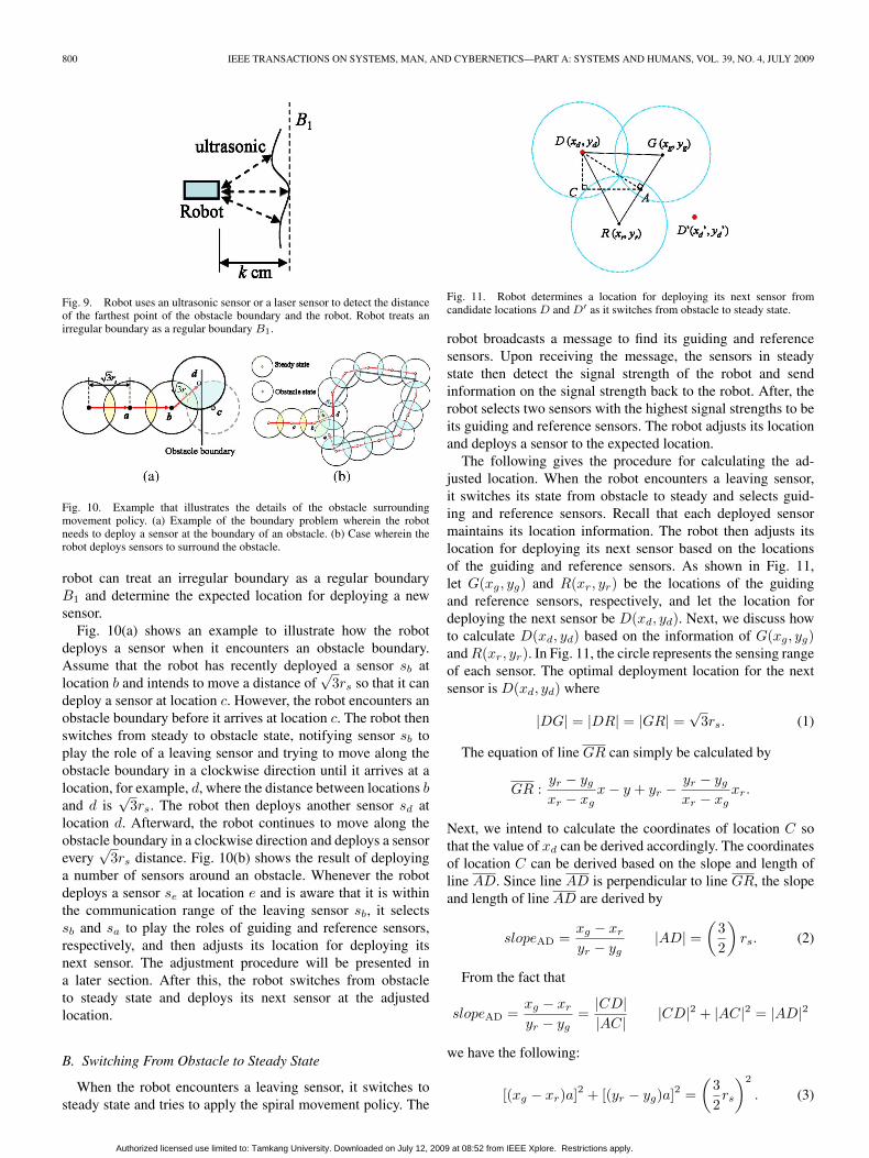
Fig. 9. Robot uses an ultrasonic sensor or a laser sensor to detect the distanceof the farthest point of the obstacle boundary and the robot. Robot treats anirregular boundary as a regular boundary B1.

Fig. 10. Example that illustrates the details of the obstacle surroundingmovement policy. (a) Example of the boundary problem wherein the robotneeds to deploy a sensor at the boundary of an obstacle. (b) Case wherein therobot deploys sensors to surround the obstacle.

robot can treat an irregular boundary as a regular boundaryB1 and determine the expected location for deploying a newsensor.

Fig. 10(a) shows an example to illustrate how the robotdeploys a sensor when it encounters an obstacle boundary.Assume that the robot has recently deployed a sensor sb atlocation b and intends to move a distance of

√3rs so that it can

deploy a sensor at location c. However, the robot encounters anobstacle boundary before it arrives at location c. The robot thenswitches from steady to obstacle state, notifying sensor sb toplay the role of a leaving sensor and trying to move along theobstacle boundary in a clockwise direction until it arrives at alocation, for example, d, where the distance between locations band d is

√3rs. The robot then deploys another sensor sd at

location d. Afterward, the robot continues to move along theobstacle boundary in a clockwise direction and deploys a sensorevery

√3rs distance. Fig. 10(b) shows the result of deploying

a number of sensors around an obstacle. Whenever the robotdeploys a sensor se at location e and is aware that it is withinthe communication range of the leaving sensor sb, it selectssb and sa to play the roles of guiding and reference sensors,respectively, and then adjusts its location for deploying itsnext sensor. The adjustment procedure will be presented ina later section. After this, the robot switches from obstacleto steady state and deploys its next sensor at the adjustedlocation.

B. Switching From Obstacle to Steady State

When the robot encounters a leaving sensor, it switches tosteady state and tries to apply the spiral movement policy. The

Fig. 11. Robot determines a location for deploying its next sensor fromcandidate locations D and D′ as it switches from obstacle to steady state.

robot broadcasts a message to find its guiding and referencesensors. Upon receiving the message, the sensors in steadystate then detect the signal strength of the robot and sendinformation on the signal strength back to the robot. After, therobot selects two sensors with the highest signal strengths to beits guiding and reference sensors. The robot adjusts its locationand deploys a sensor to the expected location.

The following gives the procedure for calculating the ad-justed location. When the robot encounters a leaving sensor,it switches its state from obstacle to steady and selects guid-ing and reference sensors. Recall that each deployed sensormaintains its location information. The robot then adjusts itslocation for deploying its next sensor based on the locationsof the guiding and reference sensors. As shown in Fig. 11,let G(xg, yg) and R(xr, yr) be the locations of the guidingand reference sensors, respectively, and let the location fordeploying the next sensor be D(xd, yd). Next, we discuss howto calculate D(xd, yd) based on the information of G(xg, yg)and R(xr, yr). In Fig. 11, the circle represents the sensing rangeof each sensor. The optimal deployment location for the nextsensor is D(xd, yd) where

|DG| = |DR| = |GR| =√

3rs. (1)

The equation of line GR can simply be calculated by

GR :yr − yg

xr − xgx − y + yr − yr − yg

xr − xgxr.

Next, we intend to calculate the coordinates of location C sothat the value of xd can be derived accordingly. The coordinatesof location C can be derived based on the slope and length ofline AD. Since line AD is perpendicular to line GR, the slopeand length of line AD are derived by

slopeAD =xg − xr

yr − yg|AD| =

(32

)rs. (2)

From the fact that

slopeAD =xg − xr

yr − yg=

|CD||AC| |CD|2 + |AC|2 = |AD|2

we have the following:

[(xg − xr)a]2 + [(yr − yg)a]2 =(

32rs

)2

. (3)



According to (3), the value of a is

a =3rs

2√

(xg − xr)2 + (yr − yg)2. (4)

The value of xd can therefore be derived based on (3)and (4):

xd =xr + xy

2− a(xg − xr).

Similarly, the value of yd can be derived using

yd =yr + yg

2+ a(yr − yg).

Note that the two locations D and D′ both satisfy (1), as shownin Fig. 11. The robot selects a location Dnext closest to the lastdeployed sensor from candidates D and D′.

Fig. 8 shows an example of the robot switching from obstacleto steady state. In Fig. 8(a), the robot finds the leaving sensor s3

and switches its state from obstacle to steady. After, the robotbroadcasts a message to neighboring steady sensors. Uponreceiving the signal strength reports from the neighboring sen-sors, the robot selects sensor s3 that has the strongest strength asits guiding sensor and selects sensor s4 as its reference sensor.Then, the robot adjusts its location and deploys sensor s28.After this, the robot applies the deployment protocol designedfor steady state. As shown in Fig. 8(b), the robot deployssensors from s28 up to s36.

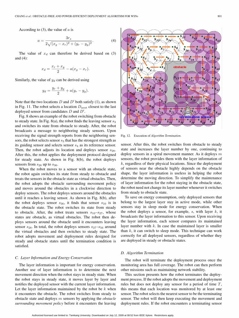
When the robot moves to a sensor with an obstacle state,the robot again switches its state from steady to obstacle andtreats the sensors in the obstacle state as virtual obstacles. Then,the robot adopts the obstacle surrounding movement policyand moves around the obstacles in a clockwise direction todeploy sensors. The robot deploys sensors around the obstaclesuntil it reaches a leaving sensor. As shown in Fig. 8(b), afterthe robot deploys sensor s36, it finds that sensor s10 is inthe obstacle state. The robot switches its state from steadyto obstacle. After, the robot treats sensors s10–s27, whosestates are obstacle, as virtual obstacles. The robot then de-ploys sensors around the obstacle until it encounters leavingsensor s28. In total, the robot deploys sensors s37–s56 aroundthe virtual obstacles and then switches to steady state. Therobot adopts movement and deployment rules designed forsteady and obstacle states until the termination condition issatisfied.

C. Layer Information and Energy Conservation

The layer information is important for energy conservation.Another use of layer information is to determine the nextmovement direction when the robot stays in steady state. Whenthe robot stays in steady state, it moves layer by layer andnotifies the deployed sensor with the current layer information.Let the layer information maintained by the robot be k whenit encounters the obstacle. The robot switches from steady toobstacle state and deploys m sensors by applying the obstaclesurrounding movement policy before it encounters the leaving

Fig. 12. Execution of Algorithm Termination.

sensor. After this, the robot switches from obstacle to steadystate and increases the layer number by one, continuing todeploy sensors in a spiral movement manner. As it deploys msensors, the robot provides them with the layer information ofk, regardless of their physical locations. Since the deploymentof sensors near the obstacle highly depends on the obstacleshape, the layer information is useless in helping the robotdetermine the moving direction. To simplify the maintenanceof layer information for the robot staying in the obstacle state,the robot need not change its layer number whenever it switchesfrom steady to obstacle state.

To save on energy consumption, only deployed sensors thatbelong to the largest layer stay in active mode, while othersensors stay in sleep mode for energy conservation. Whenthe robot deploys a sensor, for example, s, with layer k, itbroadcasts the layer information to this sensor. Upon receivingthe layer information, each sensor compares its maintainedlayer number with k. In case the maintained layer is smallerthan k, it can switch to sleep mode. This technique can workcorrectly for all deployed sensors, regardless of whether theyare deployed in steady or obstacle states.

D. Algorithm Termination

The robot will terminate the deployment process once themonitoring area has full coverage. The robot can then performother missions such as maintaining network stability.

This section presents how the robot terminates the deploy-ment process. If the robot adopts the movement and deploymentrules but does not deploy any sensor for a period of time T ,this means that each location was monitored by at least onesensor. The robot selects the nearest sensor to be the terminatingsensor. The robot will then keep executing the movement anddeployment rules. If the robot encounters a terminating sensor



Fig. 13. Considered monitoring areas that might contain obstacles.(a) Scenario 1: Rectangular area. (b) Scenario 2: Circular area. (c) Scenario 3:U-shaped obstacle existing in the rectangular area. (d) Scenario 4: X-shapedobstacle existing in the rectangular area. (e) Scenario 5: Multiple obstaclesexisting in the rectangular area.

twice but does not deploy any sensor in the monitoring field,the robot terminates the deployment process. As shown inFig. 12, after a period of time T , the robot does not deployany sensor on the monitoring field. Next, it selects sensor s49

as the terminating sensor. The robot will then keep executingthe movement and deployment rules. When the robot encoun-ters sensor s49 again, the robot terminates the deploymentprocess.

E. Robot-Deployment Algorithm

The following gives a formal description of the proposedrobot-deployment algorithm.

Notations:si: the sensor that its ID = i, i ∈ Z+.sg: guiding sensorss: initiatorse: leaving sensorsr: reference sensorst: terminating sensorC_R, cri: the current round of the robot and si.

TABLE ISIMULATION PARAMETERS

Fig. 14. Average number of deployed sensors in different monitoring areas.

C_D, cdi: the current direction of the robot and si.C_S, csi: the current state of the robot and si.(0) Initialization

set dm = {0, 5/3π, 4/3π, π, 2/3π, 1/3π}, 1 ≤ m ≤ 6.set C_R = 0, C_S = steady_state,Drop a sensor s1

If (no obstacle encounters) thenC_S = steady_state

elseC_S = obstacle_state

(1) Case 1: C_S = steady_stateIf (new round begins: C_R = end or a round) then

If (C_R �= 0 and C_R �= 1) thenbroadcast sleep_msg〈C_R〉

produce Dk={dk1 , dk−1

2 , dk3 , dk

4 , dk5 , dk

6} through C_Rthen robot deploys sensors according to Dk

else (C_R �= end or a round)send record_msg〈C_R,C_D,C_S〉 to si−1

select sg and sr by broadcasting search_beaconrobot moves in C_D direction listed in Dk for adistance of

√3rs and deploy si

If (no sensors deployed during period time T ) thensend termination_msg to sg as st

If (robot encounters st again without deploying anysensor)



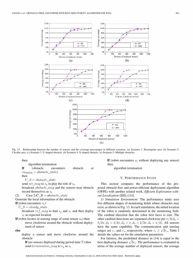
Fig. 15. Relationship between the number of sensors and the coverage percentages in different scenarios. (a) Scenario 1: Rectangular area. (b) Scenario 2:Circular area. (c) Scenario 3: U-shaped obstacle. (d) Scenario 4: X-shaped obstacle. (e) Scenario 5: Multiple obstacles.

thenalgorithm termination

If (obstacle encounters obstacle orcsMRDS = obstacle_state)then

C_S = obstacle_statesend set_msg to sg to play the role of ss

broadcast obstacle_msg and the sensors near obstaclerecord themselves as se

(2) Case 2:C_S = obstacle_stateGenerate the local information of the obstacleIf (robot encounters se)

C_S = steady_statebroadcast ref_msg to find sg and sr and then deploysi at expected location

If (robot locates in sensing range of some sensor sk) thenmove clockwise around the obstacle without deploy-ment of sensor

elsedeploy a sensor and move clockwise around theobstacle

If (no sensors deployed during period time T ) thensend termination_msg to sg as st

If (robot encounters st without deploying any sensor)then

algorithm termination

V. PERFORMANCE STUDY

This section compares the performance of the pro-posed obstacle-free and power-efficient deployment algorithm(OFPE) with another related work, Efficient Exploration with-out Localization (EEL) [14].

1) Simulation Environment: The performance study usesfive different shapes of monitoring fields where obstacles mayexist, as shown in Fig. 13. In each simulation, the initial locationof the robot is randomly determined in the monitoring field.The cardinal direction that the robot first faces is east. Theother cardinal directions are separated clockwise per π/3(d2 =5/3π, d3 = 4/3π, d4 = π, d5 = 2/3π, d6 = π/3). All sensorshave the same capability. The communication and sensingranges are rc and rs, respectively, where rc ≥ √

3rs. Table Idetails the values set for the simulation parameters.

For fairness, the predefined distance in [14] is equal to thebest deploying distance

√3rs. The performance is evaluated in

terms of the average number of deployed sensors, the average



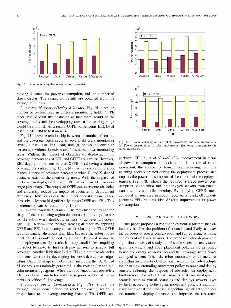
Fig. 16. Average moving distance in various scenarios.

moving distance, the power consumption, and the number ofcheck circles. The simulation results are obtained from theaverage of 20 runs.

2) Average Number of Deployed Sensors: Fig. 14 shows thenumber of sensors used in different monitoring fields. OFPEtakes into account the obstacles so that there would be nocoverage holes and the overlapping area of the sensing rangewould be minimal. As a result, OFPE outperforms EEL by atleast 28.64% and at best 44.41%.

Fig. 15 shows the relationship between the number of sensorsand the coverage percentages in several different monitoringareas. In particular, Fig. 15(a) and (b) shows the coveragepercentage without the existence of obstacles in two monitoringareas. Without the impact of obstacles on deployment, thecoverage percentages of EEL and OFPE are similar. However,EEL deploys more sensors than OFPE in achieving a similarcoverage percentage. Fig. 15(c), (d), and (e) shows the perfor-mance in terms of coverage percentage when U- and X-shapedobstacles exist in the monitoring areas. With the impacts ofobstacles on deployment, the OFPE outperforms EEL in cov-erage percentage. The proposed OFPE can overcome obstaclesand efficiently reduce the impact of obstacles in deploymentefficiency. However, in case the number of obstacles increases,these obstacles would significantly impact OFPE and EEL. Thisphenomenon can be found in Fig. 15(e).

3) Average Moving Distance: The movement policy and theshape of the monitoring region determine the moving distancefor the robot when deploying sensors to achieve full cover-age. Fig. 16 shows the average moving distance by applyingOFPE and EEL in a rectangular or circular region. The OFPErequires smaller distances than EEL because the robot move-ment of EEL is only guided by a single deployed sensor, sothis deployment easily results in many small holes, requiringthe robot to move to further deploy sensors to achieve fullcoverage. Another limitation is that EEL did not take obstaclesinto consideration in developing its robot-deployment algo-rithm. Different shapes of obstacles, including the U, X, andM shapes, are randomly generated in the rectangular and cir-cular monitoring regions. When the robot encounters obstacles,EEL results in many holes and thus requires additional move-ments to achieve full coverage.

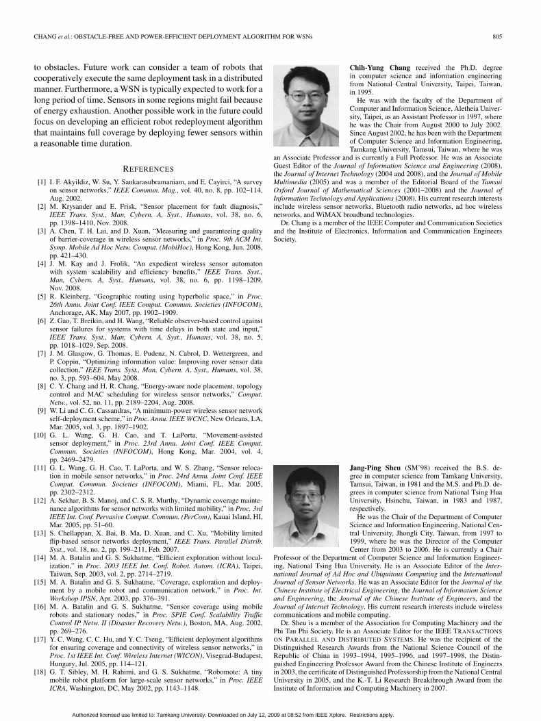
4) Average Power Consumption: Fig. 17(a) shows theaverage power consumption of robot movement, which isproportional to the average moving distance. The OFPE out-

Fig. 17. Power consumption of robot movements and communications.(a) Power consumption in robot movements. (b) Power consumption incommunications.

performs EEL by a 48.67%–63.13% improvement in termsof power consumption. In addition to the factor of robotmovement, the number of transmitting, receiving, and idlelistening packets created during the deployment process alsoimpacts the power consumption of the robot and the deployedsensors. Fig. 17(b) shows the required average power con-sumption of the robot and the deployed sensors from packettransmissions and idle listening. By applying OFPE, mostdeployed sensors stay in sleep mode. As a result, OFPE out-performs EEL by a 64.54%–82.09% improvement in powerconsumption.

VI. CONCLUSION AND FUTURE WORK

This paper proposes a robot-deployment algorithm that ef-ficiently handles the problem of obstacles and likely achievesthe purposes of power conservation and full coverage with thedeployment of fewer sensors. The proposed robot-deploymentalgorithm consists of steady and obstacle states. In steady state,spiral movement and node placement policies are proposedto achieve energy conservation and full coverage using fewerdeployed sensors. When the robot encounters an obstacle, itsalgorithm switches to obstacle state wherein the robot adoptsthe obstacle surrounding movement policy to move and deploysensors, reducing the impacts of obstacles on deployment.Furthermore, the robot treats sensors that are deployed inobstacle state as virtual obstacles and deploys sensors layerby layer according to the spiral movement policy. Simulationresults show that the proposed algorithm significantly reducesthe number of deployed sensors and improves the resistance



to obstacles. Future work can consider a team of robots thatcooperatively execute the same deployment task in a distributedmanner. Furthermore, a WSN is typically expected to work for along period of time. Sensors in some regions might fail becauseof energy exhaustion. Another possible work in the future couldfocus on developing an efficient robot redeployment algorithmthat maintains full coverage by deploying fewer sensors withina reasonable time duration.

REFERENCES

[1] I. F. Akyildiz, W. Su, Y. Sankarasubramaniam, and E. Cayirci, “A surveyon sensor networks,” IEEE Commun. Mag., vol. 40, no. 8, pp. 102–114,Aug. 2002.

[2] M. Krysander and E. Frisk, “Sensor placement for fault diagnosis,”IEEE Trans. Syst., Man, Cybern. A, Syst., Humans, vol. 38, no. 6,pp. 1398–1410, Nov. 2008.

[3] A. Chen, T. H. Lai, and D. Xuan, “Measuring and guaranteeing qualityof barrier-coverage in wireless sensor networks,” in Proc. 9th ACM Int.Symp. Mobile Ad Hoc Netw. Comput. (MobiHoc), Hong Kong, Jun. 2008,pp. 421–430.

[4] J. M. Kay and J. Frolik, “An expedient wireless sensor automatonwith system scalability and efficiency benefits,” IEEE Trans. Syst.,Man, Cybern. A, Syst., Humans, vol. 38, no. 6, pp. 1198–1209,Nov. 2008.

[5] R. Kleinberg, “Geographic routing using hyperbolic space,” in Proc.26th Annu. Joint Conf. IEEE Comput. Commun. Societies (INFOCOM),Anchorage, AK, May 2007, pp. 1902–1909.

[6] Z. Gao, T. Breikin, and H. Wang, “Reliable observer-based control againstsensor failures for systems with time delays in both state and input,”IEEE Trans. Syst., Man, Cybern. A, Syst., Humans, vol. 38, no. 5,pp. 1018–1029, Sep. 2008.

[7] J. M. Glasgow, G. Thomas, E. Pudenz, N. Cabrol, D. Wettergreen, andP. Coppin, “Optimizing information value: Improving rover sensor datacollection,” IEEE Trans. Syst., Man, Cybern. A, Syst., Humans, vol. 38,no. 3, pp. 593–604, May 2008.

[8] C. Y. Chang and H. R. Chang, “Energy-aware node placement, topologycontrol and MAC scheduling for wireless sensor networks,” Comput.Netw., vol. 52, no. 11, pp. 2189–2204, Aug. 2008.

[9] W. Li and C. G. Cassandras, “A minimum-power wireless sensor networkself-deployment scheme,” in Proc. Annu. IEEE WCNC, New Orleans, LA,Mar. 2005, vol. 3, pp. 1897–1902.

[10] G. L. Wang, G. H. Cao, and T. LaPorta, “Movement-assistedsensor deployment,” in Proc. 23rd Annu. Joint Conf. IEEE Comput.Commun. Societies (INFOCOM), Hong Kong, Mar. 2004, vol. 4,pp. 2469–2479.

[11] G. L. Wang, G. H. Cao, T. LaPorta, and W. S. Zhang, “Sensor reloca-tion in mobile sensor networks,” in Proc. 24rd Annu. Joint Conf. IEEEComput. Commun. Societies (INFOCOM), Miami, FL, Mar. 2005,pp. 2302–2312.

[12] A. Sekhar, B. S. Manoj, and C. S. R. Murthy, “Dynamic coverage mainte-nance algorithms for sensor networks with limited mobility,” in Proc. 3rdIEEE Int. Conf. Pervasive Comput. Commun. (PerCom), Kauai Island, HI,Mar. 2005, pp. 51–60.

[13] S. Chellappan, X. Bai, B. Ma, D. Xuan, and C. Xu, “Mobility limitedflip-based sensor networks deployment,” IEEE Trans. Parallel Distrib.Syst., vol. 18, no. 2, pp. 199–211, Feb. 2007.

[14] M. A. Batalin and G. S. Sukhatme, “Efficient exploration without local-ization,” in Proc. 2003 IEEE Int. Conf. Robot. Autom. (ICRA), Taipei,Taiwan, Sep. 2003, vol. 2, pp. 2714–2719.

[15] M. A. Batalin and G. S. Sukhatme, “Coverage, exploration and deploy-ment by a mobile robot and communication network,” in Proc. Int.Workshop IPSN, Apr. 2003, pp. 376–391.

[16] M. A. Batalin and G. S. Sukhatme, “Sensor coverage using mobilerobots and stationary nodes,” in Proc. SPIE Conf. Scalability TrafficControl IP Netw. II (Disaster Recovery Netw.), Boston, MA, Aug. 2002,pp. 269–276.

[17] Y. C. Wang, C. C. Hu, and Y. C. Tseng, “Efficient deployment algorithmsfor ensuring coverage and connectivity of wireless sensor networks,” inProc. 1st IEEE Int. Conf. Wireless Internet (WICON), Visegrad-Budapest,Hungary, Jul. 2005, pp. 114–121.

[18] G. T. Sibley, M. H. Rahimi, and G. S. Sukhatme, “Robomote: A tinymobile robot platform for large-scale sensor networks,” in Proc. IEEEICRA, Washington, DC, May 2002, pp. 1143–1148.

Chih-Yung Chang received the Ph.D. degreein computer science and information engineeringfrom National Central University, Taipei, Taiwan,in 1995.

He was with the faculty of the Department ofComputer and Information Science, Aletheia Univer-sity, Taipei, as an Assistant Professor in 1997, wherehe was the Chair from August 2000 to July 2002.Since August 2002, he has been with the Departmentof Computer Science and Information Engineering,Tamkang University, Tamsui, Taiwan, where he was

an Associate Professor and is currently a Full Professor. He was an AssociateGuest Editor of the Journal of Information Science and Engineering (2008),the Journal of Internet Technology (2004 and 2008), and the Journal of MobileMultimedia (2005) and was a member of the Editorial Board of the TamsuiOxford Journal of Mathematical Sciences (2001–2008) and the Journal ofInformation Technology and Applications (2008). His current research interestsinclude wireless sensor networks, Bluetooth radio networks, ad hoc wirelessnetworks, and WiMAX broadband technologies.

Dr. Chang is a member of the IEEE Computer and Communication Societiesand the Institute of Electronics, Information and Communication EngineersSociety.

Jang-Ping Sheu (SM’98) received the B.S. de-gree in computer science from Tamkang University,Tamsui, Taiwan, in 1981 and the M.S. and Ph.D. de-grees in computer science from National Tsing HuaUniversity, Hsinchu, Taiwan, in 1983 and 1987,respectively.

He was the Chair of the Department of ComputerScience and Information Engineering, National Cen-tral University, Jhongli City, Taiwan, from 1997 to1999, where he was the Director of the ComputerCenter from 2003 to 2006. He is currently a Chair

Professor of the Department of Computer Science and Information Engineer-ing, National Tsing Hua University. He is an Associate Editor of the Inter-national Journal of Ad Hoc and Ubiquitous Computing and the InternationalJournal of Sensor Networks. He was an Associate Editor for the Journal of theChinese Institute of Electrical Engineering, the Journal of Information Scienceand Engineering, the Journal of the Chinese Institute of Engineers, and theJournal of Internet Technology. His current research interests include wirelesscommunications and mobile computing.

Dr. Sheu is a member of the Association for Computing Machinery and thePhi Tau Phi Society. He is an Associate Editor for the IEEE TRANSACTIONS

ON PARALLEL AND DISTRIBUTED SYSTEMS. He was the recipient of theDistinguished Research Awards from the National Science Council of theRepublic of China in 1993–1994, 1995–1996, and 1997–1998, the Distin-guished Engineering Professor Award from the Chinese Institute of Engineersin 2003, the certificate of Distinguished Professorship from the National CentralUniversity in 2005, and the K.-T. Li Research Breakthrough Award from theInstitute of Information and Computing Machinery in 2007.



Yu-Chieh Chen received the B.S. degree in com-puter science and information engineering fromMing Chuan University, Taipei, Taiwan, in 2005 andthe M.S. degree in computer science and informa-tion engineering from Tamkang University, Tamsui,Taiwan, in 2007, where he has been working towardthe Ph.D. degree in the Department of ComputerScience and Information Engineering since then.

His research domains include wireless sensor net-works, ad hoc wireless networks, mobile/wirelesscomputing, and WiMAX.

Mr. Chen won many scholarships in Taiwan and participated in manywireless sensor networking projects.

Sheng-Wen Chang received the B.S. degree incomputer science and information engineering fromTamkang University, Tamsui, Taiwan, in 2004,where he has been working toward the Ph.D. degreesince 2005 in the Department of Computer Scienceand Information Engineering.

He has published extensively in the wireless net-working area. His research interests are WiMAX,wireless sensor networks, Bluetooth radio networks,wireless mesh networks, and ad hoc wireless net-works, concerning both theoretic and algorithm

design.Mr. Chang is a student member of the IEEE Computer and Communication

Societies and the Institute of Electronics, Information and CommunicationEngineers Society. He has won many scholarships in Taiwan and participatedin many Bluetooth and wireless sensor networking projects.


An Obstacle-Free and Power-Efficient Deployment Algorithm for Wireless Sensor Networks

Documents

Transcript of An Obstacle-Free and Power-Efficient Deployment Algorithm for Wireless Sensor Networks