Mobility Limited Flip-based Sensor Networks

Deployment

Sriram Chellappan, Xiaole Bai, Bin Ma, Dong Xuan and Changqing Xu

Abstract

An important phase of sensor networks operation is deployment of sensors in the field of interest. Critical

goals during sensor networks deployment include coverage, connectivity, load balancing etc. A class of work has

recently appeared, where mobility in sensors is leveraged to meet deployment objectives. In this paper, we study

deployment of sensor networks using mobile sensors. The distinguishing feature of our work is that the sensors in

our model have limited mobilities. More specifically, the mobility in the sensors we consider is restricted to a flip,

where the distance of the flip is bounded. We call such sensors as flip-based sensors. Given an initial deployment

of flip-based sensors in a field, our problem is to determine a movement plan for the sensors in order to maximize

the sensor network coverage, and minimize the number of flips. We propose a minimum-cost maximum-flow based

solution to this problem. We prove that our solution optimizes both the coverage and the number of flips. We

also study the sensitivity of coverage and the number of flips to flip distance under different initial deployment

distributions of sensors. We observe that increased flip distance achieves better coverage, and reduces the number

of flips required per unit increase in coverage. However, such improvements are constrained by initial deployment

distributions of sensors, due to the limitations on sensor mobility.

Index Terms

Sensor Networks Deployment, Limited Mobility, Flip-based Sensors.

Sriram Chellappan, Xiaole Bai and Dong Xuan are with The Dept. of Computer Science and Engineering, The Ohio-State University,Columbus, OH 43210, U.S.A. E-mail: {chellapp, baixia, xuan}@cse.ohio-state.edu. Bin Ma is with The Dept. of Computer Science, Universityof Western Ontario, London, ON N6A5B7, Canada. Email: bma@csd.uwo.ca. Changqing Xu is with The Dept. of Electronic Engineering,Shanghai Jiao Tong University, China. Email: cqxu@sjtu.edu.cn.

This work was partially supported by NSF under grants No. ACI-0329155 and CAREER Award CCF-0546668. Any opinions, findingsand conclusions or recommendations expressed in this material are those of the authors and do not necessarily reflect the views of NSF.

2

I. INTRODUCTION

Sensor networks deployment in an important phase of sensor networks operation. A host of works has

appeared in this realm in the recent past [1], [2], [3], [4], [5], [6], [7], [8], [9]. One of the important

goals of sensor networks deployment is to ensure that the sensors meet critical network objectives that

may include coverage, connectivity, load balancing etc. When a number of sensors are to be deployed,

it is not practical to manually position sensors in desired locations. In many situations, the sensors are

deployed from a remote site (like from an airplane) that makes it very hard to control deployment.

To address this issue, a class of work has recently appeared where mobility of sensors is taken advantage

of to achieve desired deployment [1], [2], [4], [7]. Typically in such works, the sensors detect lack

of desired deployment objectives. The sensors then estimate new locations, and move to the resulting

locations. While the above works are quite novel in their approaches, the mobility of the sensors in their

models is unlimited. Specifically, if a sensor chooses to move to a desired location, it can do so without

any limitation in the movement distance.

In practice however, it is quite likely that the mobility of sensors is limited. Towards this extent, a class

of Intelligent Mobile Land Mine Units (IMLM) [10] to be deployed across battlefields have been developed

by DARPA. The IMLM units are expected to detect breaches and move to repair them. The mobility of

the IMLM units is limited. Briefly, the mobility system in [10] is based on a hopping mechanism that is

actuated by a single-cylinder combustion process. Each IMLM unit in the field carries onboard fuel tanks

and a spark initiation/ propeller system. For each hop, the fuel is metered into the combustion chamber

and ignited to propel the IMLM unit into the air. The hop distance is limited depending on the amount of

fuel and the propeller dynamics. The units include a righting and steering system for orientation during

hops. Other technologies can also assist in such mobilities, like sensors enabled with spring actuation,

external agents launching sensors after being deployed in the field etc. Such a model typically trades-off

mobility with energy consumption and cost. In many applications, the latter goals outweigh the necessity

for advanced mobilities, making such mobility models quite practical in the future.

3

In this paper, we study sensor networks deployment using sensors with limited mobilities. In our model,

sensors can flip (or hop) only once to a new location, and the flip distance is bounded. We call such sensors

as flip-based sensors. A certain number of flip-based sensors are initially deployed in the sensor network

that is clustered into multiple regions. The initial deployment may not cover all regions in the network.

Regions that do have any sensor in them are holes. In this framework, our problem is to determine an

optimal movement (or flip) plan for the sensors in order to maximize the number of regions that is covered

by at-least one sensor (or minimize the number of holes), and simultaneously minimize the total number

of sensor movements (or flips).

We propose a minimum-cost maximum-flow based solution to our deployment problem. Our approach

is to translate the sensor network at initial deployment and sensor mobility model into a graph (called

virtual graph). Regions in the sensor network are modeled as vertices, and possible sensor movement paths

between regions are modeled as edges between corresponding vertices in the virtual graph. Capacities

for the edges model the number of sensors that can flip between regions. A cost value is also assigned

to the edges to capture the number of flips between regions. Since the virtual graph models the sensor

network, our problem of optimally moving sensors to holes, can be translated as one where we want

to optimally determine flows to hole vertices in the virtual graph. The first objective of our problem,

namely determining a movement plan to maximize coverage can be translated as determining the flow

plan (a set of flows in the virtual graph) that corresponds to the maximum flow to hole vertices in the

virtual graph, without violating edge capacities. Note that, there can be more than one flow plan that can

maximize the flow in the virtual graph. Out of such flow plans, our second objective is to determine the

plan that minimizes the overall cost, which corresponds to the minimizing the number of sensor flips.

Intuitively, each flow in the flow plan (in the virtual graph) denotes a path for a sensor movement to a

hole in the sensor network. As we discuss later, the maximum flow value in the virtual graph denotes

the maximum number of holes into which a sensor can move without violating the mobility constraints,

4

while the minimum cost denotes the corresponding minimum number of sensor movements (or flips) 1.

In our solution, we translate the flow plan corresponding to the minimum cost maximum flow in the

virtual graph into a movement plan for the sensors in the region. We subsequently prove the optimality of

this movement plan. We also propose multiple approaches that sensors can adopt to execute our solution

in practice. We then perform simulations to study the sensitivity of coverage and the number of flips to

flip distance under different initial deployment distributions of sensors. We observe that increased flip

distance achieves better coverage, and reduces the number of flips required per unit increase in coverage.

However, such improvements are constrained by initial deployment distributions of sensors, due to the

limitations on sensor mobility.

The rest of our work is organized as follows. We present important related work in Section II. In Section

III, we formally define our flip-based mobility model, and our deployment problem. We then present our

solution, its properties and alternate approaches to execute our solution in Section IV. In Section V, we

present results of our performance evaluations. We present some discussions in Section VI and conclude

our paper with some final remarks in Section VII.

II. RELATED WORK

Sensor network deployment is a topic that has received significant attention in the recent past [1], [2],

[3], [4], [5], [6], [7], [8], [11], [12], [9] [13]. In this section, we focus on works related to mobility

assisted sensor networks deployment [1], [2], [4], [7]. The key objective in [1], [4], [7] is to detect holes

in the network and cover them with at least one sensor. In the approach proposed by Wang, Cao and La

Porta, in [4] the detection of holes is based on constructing Voronoi diagrams. Each sensor constructs its

own Voronoi polygon, which enables sensors to detect holes. The authors then propose three algorithms,

namely Vector-based algorithm, Voronoi-based algorithm and Minimax algorithm to maximize coverage.

In their algorithms, sensors move over a series of iterations to balance virtual forces between themselves.

They stop moving when global force balance is achieved, which corresponds to attainment of desired

1The translation will become clearer once we discuss exactly how capacities and costs are assigned in the virtual graph in Section IV-B.

5

deployment. In [1], Howard, Mataric and Sukhatme propose the idea of constructing potential fields to

maximize coverage. The fields are constructed such that each node is repelled by both obstacles and by

other nodes, thereby forcing the sensors to spread throughout the environment. In Zou and Chakrabarty’s

work in [7], all sensors in the network forward their location to a centralized node. The centralized node

determines the final positions of sensors as those positions that balance the virtual forces in the network.

In all the above works [1], [4], [7], sensors move depending on virtual forces exerted by them. In the

principle of virtual forces, sensors attract each other if they are far apart, and repel each other if they

are too close. In this approach, sensors keep moving over several iterations. In each iteration, a degree of

force balance is achieved by the sensors. After many such iterations, sensors achieve global force balance

among themselves, which in turn corresponds to attainment of desired deployment objectives. The virtual

force approach cannot work for our problem for two reasons. Sensors in our model are capable of only

a flip. The lack of continuous motion implies that even between two sensors, force balance may not be

achieved if they flip towards or apart from each other. Secondly, the virtual force approach requires a

series of iterations (a series of sensor movements) to achieve global force balance in the network. When

constrained by mobility, the virtual force approach has limited application.

Another related work is Wu and Yang’s work in [2]. In [2], the sensor network is divided into clusters.

The objective is to ensure that the number of sensors per cluster is uniform. The algorithms designed

efficiently scan the clusters in two stages (row-wise and column-wise) sequentially, and determine new

sensor locations (or clusters) in each stage. Sensors move in each stage to new clusters to achieve uniform

deployment. Intuitively, this approach has some applicability to our problem. Sensors can exchange

information row wise (along all rows) and then flip between regions in their row first. A column-wise

information exchange and flip can follow next. Clearly, coverage is improved here compared to initial

deployment. However, the final deployment in the two-stage approach will be far from optimal in terms of

both coverage and sensor flips. Optimizing coverage sequentially in row-wise and column-wise directions

results in non-optimal flips that will compromise optimality of final coverage. Due to the two-stage flip

6

sequence for sensors (row-wise and column wise), more than necessary flips can be introduced.

To summarize here, our objectives in this paper (maximizing coverage and minimizing sensor move-

ments) shares similarities with the above works [1], [2], [4], [7]. The major reason why the above

approaches do not work in our problem is due to limitations on sensor mobility. In the above works, sensors

move based on local measurements and communications. Erroneous movements made by the sensors are

eventually corrected over time, since the sensor movement distance is unlimited. In our problem, sensor

movement distance itself is a hard constraint. This means that, we are fundamentally constrained by the

movement choices available to us (compared to unlimited mobility) during deployment. The consequence

is the increased importance that each sensor flip needs to be accorded. Sensors therefore cannot just make

local decisions and flip. We need to determine a movement plan for the sensors prior to their flip, which

is the output of our solution in this paper.

III. MOBILITY MODEL AND PROBLEM DEFINITION

A. The Flip-based Sensor Mobility model

In this paper, we model sensor mobilities as a flip. That is, the motion of the sensor is in the form

of a flip (or hop) from its current location to a new one when triggered by an appropriate signal. Such

a movement can be realized in practice by propellers powered by fuels [10], coiled springs unwinding

during flips, external agents launching sensors after deployed in the field etc. In our model, sensors can

flip only once to a new location. This could be due to propeller dynamics, or the spring unable to recoil

after a flip, or the external agent launching the sensor. The distance to which a sensor can flip is limited.

The sensor can flip in a desired angle. Mechanisms in [10] can be used for orientation during flips. The

limitation in sensor mobility comes from the bound on the maximum distance they can move, which again

depends on available fuel quantity, degree of spring coil etc. We study two models of flip-based mobility.

The first is a fixed distance mobility model, while the second is a variable distance mobility model.

We denote the maximum distance a sensor can flip to as F . In the first model, the distance to which a

sensor can flip is fixed and is equal to F . We extend the above model further. Although the number of flips

7

is still one, in many cases, depending on the triggering signals, fuel can be metered variably, or the spring

can unwind only partially, or the external agent can variably adjust the flip distance during launching. In

the second model, sensors can flip to distances between 0 and F . We denote d as the basic unit of distance

flipped. We assume that F is an integral multiple of the basic unit d. Thus in the second model, sensors

can flip once to distances d, 2d, 3d, . . . nd from its current location, where nd = F . To differentiate the

above two models, we introduce the notation C to denote choice for flip distance. C = 1 denotes the first

model, where the sensor has only one fixed choice for flip distance (the maximum distance F ). C = n

denotes the second model, where the sensor has n choices for the flip distance (between d and maximum

distance F ). For the rest of the paper, unless otherwise clearly specified, the term flip distance denotes

the maximum flip distance F .

B. Problem Definition

The sensor network we study is a square field. It is divided into 2-dimensional regions, where each

region is a square of size R. A certain number of flip-based sensors are deployed initially in the network.

The initial deployment may have holes that are not covered by any sensor. In this context, our problem

statement is; Given a sensor network of size D, a desired region size R, an initial deployment of N flip-

based sensors that can flip once to a maximum distance F , our goal is to determine an optimal movement

plan for the sensors, in order to maximize the number of regions that is covered by at least one sensor,

while simultaneously minimizing the total number of flips required. The input to our problem is the initial

deployment (number of sensors per region) in the sensor network, and the mobility model of sensors. The

output is the detailed movement plan of the sensors across the regions (which sensors should move, and

where) that can achieve our desired objectives.

The region size R is contingent on the application, based on sensing/ transmission ranges of sensors,

and application demands. We assume that min{Ssen√

2, Str√

5} ≥ R, where Ssen and Str are sensing and

transmission ranges of the sensors respectively. This guarantees that if a sensor is present in a region,

every point in the region is covered by the sensor, and the sensor can communicate with sensors in each

8

of its four adjacent regions. In this paper, we first assume that the desired region size R is an integral

multiple of the basic unit of flip distance, i.e., R = m ∗ d, where m is an integer (≥ 1). We discuss the

general case of R subsequently in Section VI. We assume that each sensor knows its position. To do

so, sensors can be provisioned with GPS devices, or approaches in [14] can be applied, where sensors

are localized using sensors themselves as landmarks. In our model, the regions to which a sensor can

flip, are those in its left, right, top and bottom directions. However, those regions need not be just the

adjacent neighbors. They depend on the flip distance F . After discussing the above case, the general case,

where a sensor can flip to regions in any arbitrary direction is discussed subsequently in Section VI. The

base-station can reside anywhere as long as it is able to communicate with the sensors.

C. An Example

We illustrate our problem further with an example. Figure 1 (a) shows an instance of initial deploy-

ment in the sensor network. The shaded circles denote sensors, and the numbers denote the id of the

corresponding region in the network. The neighbors of any region are its immediate left, right, top and

bottom regions. For instance in Figure 1, the neighbors of region 6 are regions 2, 5, 7 and 10. In Figure

1 (a) after the initial deployment, regions 1, 6, 11, 12, 16 are not covered by any sensor and are thus

holes. Optimally covering such holes is the problem we address in this paper.

1

5 6

3 42

7

9 10 11 12

13 14 15 16

1

5 6

3 42

7 8

9 10 11 12

13 14 15 16

(a) (b)

8

Fig. 1. A snapshot of the sensor network and a movement plan to maximize coverage (a), and the resulting deployment (b)

The above problem is not easy to solve. For instance, consider Figure 1 (a). For ease of elucidation, let

the desired region size R = d. Let the flip distance F = d. One intuitive approach towards maximizing

9

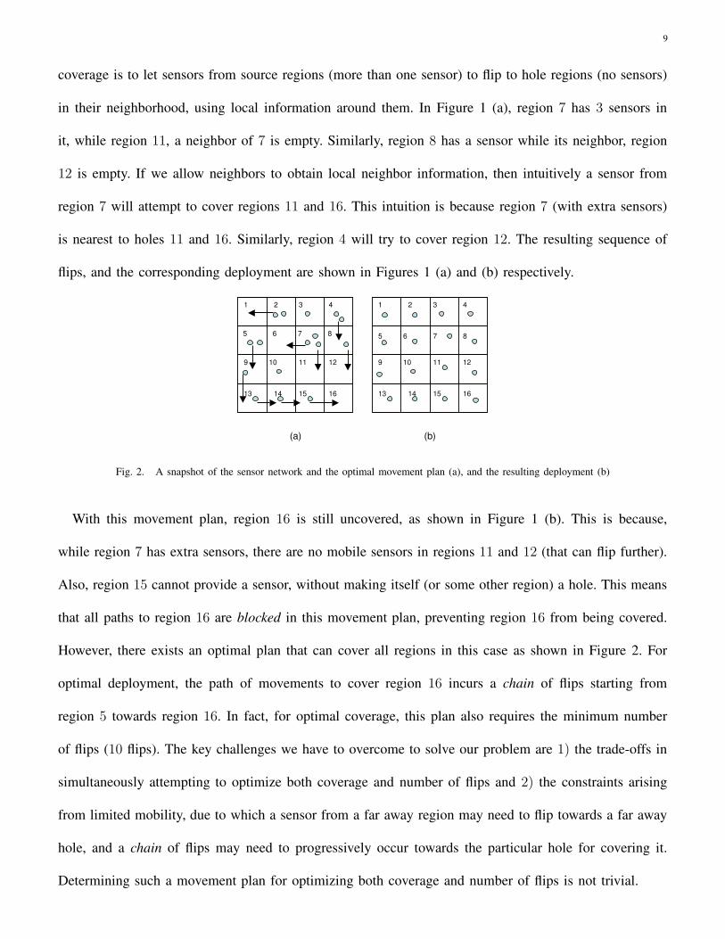
coverage is to let sensors from source regions (more than one sensor) to flip to hole regions (no sensors)

in their neighborhood, using local information around them. In Figure 1 (a), region 7 has 3 sensors in

it, while region 11, a neighbor of 7 is empty. Similarly, region 8 has a sensor while its neighbor, region

12 is empty. If we allow neighbors to obtain local neighbor information, then intuitively a sensor from

region 7 will attempt to cover regions 11 and 16. This intuition is because region 7 (with extra sensors)

is nearest to holes 11 and 16. Similarly, region 4 will try to cover region 12. The resulting sequence of

flips, and the corresponding deployment are shown in Figures 1 (a) and (b) respectively.

1 3 42

9 10 11 12

13 14 15 16

1

5 6

3 42

7 8

9 10 11 12

13 14 15 16

(a) (b)

5 6 7 8

Fig. 2. A snapshot of the sensor network and the optimal movement plan (a), and the resulting deployment (b)

With this movement plan, region 16 is still uncovered, as shown in Figure 1 (b). This is because,

while region 7 has extra sensors, there are no mobile sensors in regions 11 and 12 (that can flip further).

Also, region 15 cannot provide a sensor, without making itself (or some other region) a hole. This means

that all paths to region 16 are blocked in this movement plan, preventing region 16 from being covered.

However, there exists an optimal plan that can cover all regions in this case as shown in Figure 2. For

optimal deployment, the path of movements to cover region 16 incurs a chain of flips starting from

region 5 towards region 16. In fact, for optimal coverage, this plan also requires the minimum number

of flips (10 flips). The key challenges we have to overcome to solve our problem are 1) the trade-offs in

simultaneously attempting to optimize both coverage and number of flips and 2) the constraints arising

from limited mobility, due to which a sensor from a far away region may need to flip towards a far away

hole, and a chain of flips may need to progressively occur towards the particular hole for covering it.

Determining such a movement plan for optimizing both coverage and number of flips is not trivial.

10

IV. OUR SOLUTION

A. Design Rationale

In this paper, we propose a solution where information on number of sensors per region for all regions is

collected by the Base-station, and an optimal movement plan for the sensors is determined and forwarded

to the sensors. We propose a minimum-cost maximum-flow based solution that is executed by the Base-

station using the region information to determine the movement plan. The Base-station will then forward

the movement plan (which sensors should move and where) to corresponding sensors in the network.

Each sensor in the network will first determine its position and the region it resides in. Sensors then

forward their location information to the Base-station 2. The packets are forwarded towards the Base-

station through other neighboring regions closer to the Base-station. To do so, protocols like [15], [16],

[17] can be used, where the protocols route packets towards sinks in the network (Base-station in our

case) using shortest paths. Another solution that does not require a centralized node is to let individual

sensors collect region information, and execute our solution independently to determine the movement

plan. We discuss the latter solution in Section IV-E.

We now discuss how to translate our problem into a minimum-cost maximum-flow problem. Let us

denote regions with at least two sensors as sources. Source Regions can provide sensors (like region 5

in Figure 1 (a)), or they can be on a path between another source and a hole. Let us denote regions

with only one sensor as forwarders. Forwarder regions cannot provide sensors (otherwise, they become

holes themselves), but they can be on a path between a source and a hole (like regions 9, 13, 14, 15 in

Figure 1 (a)). Let us denote regions without any sensor as holes. Obviously holes can only accept sensors

(regions 1, 6, 11, 12 and 16). The first objective of our problem is to maximize the number of holes that

eventually have a sensor in them. Since there can be multiple sources and multiple forwarders, in the event

of maximizing the number of holes that eventually contain a sensor, there can be many possible sequences

of sensor movements. Out of such possible sequences, our second objective is to find the sequence that

2Alternatively, a region-head can be elected in each region to collect and forward information on number of sensors in their region.

11

minimizes the number of sensor movements.

If we identify regions (sources, forwarders and holes) using vertices, and incorporate path relationships

in the sensor network as edges (with appropriate constrained capacities) between the vertices, then from

a graph-theoretic perspective, our problem is a version of the multi-commodity maximum flow problem,

where the problem is to maximize flows from multiple sources to multiple sinks in a graph, while ensuring

that the capacity constraints on the edges in the graph are not violated. While obtaining the optimal plan

to maximize coverage, we also want to minimize the number of flips. That is, if we associate a cost with

each flip, we wish to minimize the overall cost of flips while still maximizing coverage. This problem

is then a version of the minimum-cost multi-commodity maximum-flow problem, where the objective is

to find paths that minimize the overall cost while still maximizing the flow. Our solution is to model the

sensor network as an appropriate graph structure (called virtual graph) following the objectives discussed

above, determine the minimum cost maximum flow plan in the virtual graph. Each flow in the flow plan

(in the virtual graph) denotes a path for a sensor movement from a source to a hole in the sensor network.

As we discuss later, the maximum flow value in the virtual graph denotes the maximum number of holes

into which a sensor can move without violating the mobility constraints, while the minimum cost denotes

the corresponding minimum number of sensor movements (or flips). We then translate the flow plan as

flip sequences in the sensor network. For the rest of the paper, if the context is clear, we will call our

solution as minimum-cost maximum-flow solution.

B. Constructing the virtual graph from the initial deployment

We now discuss the construction of the virtual graph in detail. The inputs are the initial deployment

(with N sensors), the granularity of desired coverage (region size R), flip distance (F ) and the number of

sensors per region i (ni). We denote the number of regions in the network as Q. Let GS(VS, ES) be an

undirected graph representing the sensor network. Each vertex ∈ VS represents one region in the sensor

network and each edge ∈ ES represents path relationship between regions. GS purely represents the initial

network structure (and does not reflect whether regions are sources, forwarders or holes), and as such is

12

undirected. The virtual graph (denoted by GV (VV , EV )) is constructed from GS .

The key task in constructing the virtual graph (GV ) is to first determine its vertices (the set VV )

commensurate with the status of each region as a source, forwarder or hole. Then, we have to establish

the edges (the set EV ), directions, capacities and costs in GV between the vertices. For any region i in

the sensor network, we denote its reachable regions as those to which a sensor from region i can flip to.

Obviously, the reachable regions depend on the flip distance F . In GV , edges are added between such

reachable regions. The directions of edges between vertices are based on whether the corresponding regions

are sources, forwarders or holes in the sensor network. The capacities of the edges depend on the number

of sensors in the regions, while the cost is used to quantify the number of sensor flips between regions

in the sensor network. We denote C(p, q) as the capacity, and Cost(p, q) as the cost of the edge between

vertices p and q in GV respectively. The final objective is to ensure that the minimum-cost maximum-flow

plan in GV can be translated into an optimal movement (flip) plan for sensors in the network. In the

following, we first discuss how to construct the virtual graph for a simple, yet representative basic case.

We then discuss how to construct the virtual graph for general case.

1) Constructing the virtual graph for the case R = d: In this case, the region size R is equal to the

basic unit of flip distance d. To explain the virtual graph construction process clear, we first describe it

for the case where the flip distance F = d, and C = 1. That is, the flip distance is the basic unit d and

the sensor has only one choice for flip distance. We discuss the case where F > d and C = 1, and F > d

and C = n (multiple choices) subsequently. The case where R > d is discussed in Section IV-B.2.

a) Construction when F = d and C = 1: In the virtual graph, each region (of size R) is represented

by 3 vertices. For each region i, we create a vertex for it in GV called base vertex, denoted as vbi . The

base vertex vbi of region i keeps track on the number of sensors that are in region i. For each region, we

need to keep track of the number of sensors from other regions that have flipped to it, and the number of

sensors that have flipped from this region to other regions. The former task is accomplished by creating

an in vertex, and the latter is accomplished by creating an out vertex for each region. For each vertex i,

13

its in vertex in the virtual graph is denoted as vini and its out vertex is denoted as vout

i .

1v1

b

0 infv1

outv1in

inf

Hole

1v2

b

2v2

out

Source

v2in

Fig. 3. The Virtual Graph with only regions 1 and 2 in it

Having established the vertices, we now discuss how edges (and their capacities) are added between

vertices in GV . Recall that each region that has ≥ 2 sensors is considered a source, and each region that

has ≥ 1 sensor is considered a forwarder. We are interested in how to optimally push sensors from such

regions. For such regions, an edge is added from the corresponding vbi to vin

i with capacity ni − 1. The

interpretation of this is that when attempting to determine the flow from the base vertex (vbi ), at least

one sensor will remain in the corresponding region i. Then an edge with capacity ni is added from the

same vini to vout

i . This ensures that it is possible for up to ni sensors in this region to flip from it. Recall

the example in Figure 1 (a). Region 2 is a source. The GV construction corresponding to this region is

shown in Figure 3, where there is an edge with capacity n2 − 1 = 1 from vertex vb2

to vin2

, and an edge

of capacity ni = 2 from vin2

to vout2

. Other source and forwarder regions are treated similarly in GV .

Each region that has 0 sensors is considered a hole. We are interested in how to optimally absorb

sensors in such regions. For holes, an edge is added from the corresponding v ini to base vertex vb

i with

edge capacity equal to 1. This is to allow a maximum of one sensor into the base vertex vbi of hole region

i. If a sensor flips to this hole, the hole is then covered, and no other sensor needs to flip to this region.

Then an edge with capacity 0 is added from the same vini to vout

i . This is because a sensor that moves

into a hole will be not able to flip further 3. Recall again from the example in Figure 1 (a). Region 1 is

a hole. In Figure 3, there is an edge with capacity 1 from vertex vin1

vertex to vb1, and edge of capacity 0

3In practice an edge with capacity 0 need not be specifically added. We do so to retain the symmetricity in the virtual graph construction.

14

from vini to the vout

1. Other holes are treated similarly in GV . We now have,

∀vini and vout

i ∈ VV , C (vini , vout

i ) = ni (1)

∀vbi and vin

i ∈ VV | ni > 0, C (vbi , v

ini ) = ni − 1 (2)

∀vini and vb

i ∈ VV | ni = 0, C (vini , vb

i ) = 1. (3)

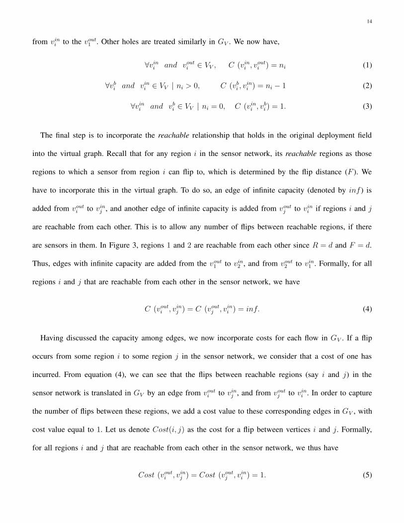
The final step is to incorporate the reachable relationship that holds in the original deployment field

into the virtual graph. Recall that for any region i in the sensor network, its reachable regions as those

regions to which a sensor from region i can flip to, which is determined by the flip distance (F ). We

have to incorporate this in the virtual graph. To do so, an edge of infinite capacity (denoted by inf ) is

added from vouti to vin

j , and another edge of infinite capacity is added from voutj to vin

i if regions i and j

are reachable from each other. This is to allow any number of flips between reachable regions, if there

are sensors in them. In Figure 3, regions 1 and 2 are reachable from each other since R = d and F = d.

Thus, edges with infinite capacity are added from the vout1

to vin2

, and from vout2

to vin1

. Formally, for all

regions i and j that are reachable from each other in the sensor network, we have

C (vouti , vin

j ) = C (voutj , vin

i ) = inf. (4)

Having discussed the capacity among edges, we now incorporate costs for each flow in GV . If a flip

occurs from some region i to some region j in the sensor network, we consider that a cost of one has

incurred. From equation (4), we can see that the flips between reachable regions (say i and j) in the

sensor network is translated in GV by an edge from vouti to vin

j , and from voutj to vin

i . In order to capture

the number of flips between these regions, we add a cost value to these corresponding edges in GV , with

cost value equal to 1. Let us denote Cost(i, j) as the cost for a flip between vertices i and j. Formally,

for all regions i and j that are reachable from each other in the sensor network, we thus have

Cost (vouti , vin

j ) = Cost (voutj , vin

i ) = 1. (5)

15

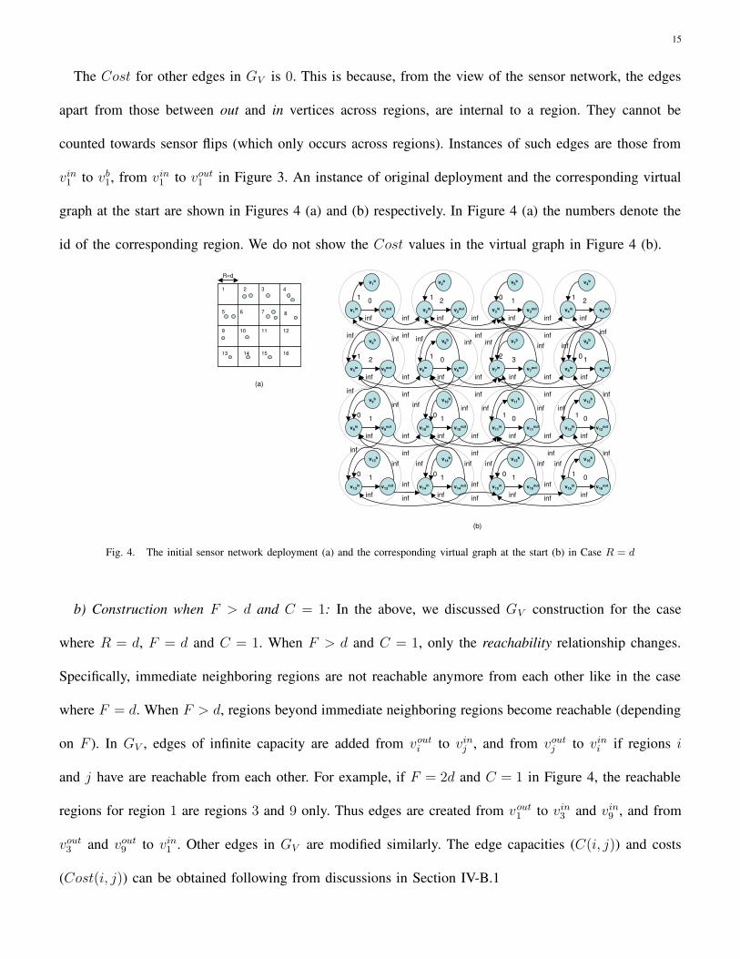
The Cost for other edges in GV is 0. This is because, from the view of the sensor network, the edges

apart from those between out and in vertices across regions, are internal to a region. They cannot be

counted towards sensor flips (which only occurs across regions). Instances of such edges are those from

vin1

to vb1, from vin

1to vout

1in Figure 3. An instance of original deployment and the corresponding virtual

graph at the start are shown in Figures 4 (a) and (b) respectively. In Figure 4 (a) the numbers denote the

id of the corresponding region. We do not show the Cost values in the virtual graph in Figure 4 (b).

1

5 6

3 42

7

9 10 11 12

13 14 15 16

(a)

v1b

v1outv1

in v2outv2

in v3outv3

in v4outv4

in

v4bv3

bv2b

1 0

inf

1 2

inf

0 1

inf

1 2

inf

0 1

inf

0 1

inf

1 0

inf

1 0

inf

0 1

inf

0 1

inf

0 1

inf

1 0

inf

1 2

inf

1 0

inf

2 3

inf

0 1

inf

inf

infinf

infinf

inf inf inf

infinfinf

inf

inf inf

inf inf

inf

infinfinf

infinfinfinfinf

inf

inf inf

inf

infinfinfinfinfinf

infinfinf infinfinf

infinfinfinf infinfinf

v5b

v5outv5

in v6outv6

in v7outv7

in v8outv8

in

v8bv7

bv6b

v9b

v9outv9

in v10outv10

in v11outv11

in v12outv12

in

v12bv11

bv10b

v13b

v13outv13

in v14outv14

in v15outv15

in v16outv16

in

v16bv15

bv14b

(b)

R=d

8

Fig. 4. The initial sensor network deployment (a) and the corresponding virtual graph at the start (b) in Case R = d

b) Construction when F > d and C = 1: In the above, we discussed GV construction for the case

where R = d, F = d and C = 1. When F > d and C = 1, only the reachability relationship changes.

Specifically, immediate neighboring regions are not reachable anymore from each other like in the case

where F = d. When F > d, regions beyond immediate neighboring regions become reachable (depending

on F ). In GV , edges of infinite capacity are added from vouti to vin

j , and from voutj to vin

i if regions i

and j have are reachable from each other. For example, if F = 2d and C = 1 in Figure 4, the reachable

regions for region 1 are regions 3 and 9 only. Thus edges are created from vout1

to vin3

and vin9

, and from

vout3

and vout9

to vin1

. Other edges in GV are modified similarly. The edge capacities (C(i, j)) and costs

(Cost(i, j)) can be obtained following from discussions in Section IV-B.1

16

c) Construction when F > d and C = n: In this case again, only the reachability relationship changes.

Recall that if F > d and C = n, the distance of flip can be d, 2d, 3d, . . . nd, where F = nd. For example

if F = 2d and C = 2 in Figure 4, then the reachable regions of region 1 are regions 2, 3, 5 and 9. Thus,

apart from existing edges, edges are also added from vout1

to vin3

and vin9

, and from vout3

and vout9

to vin1

.

Other edges, capacities and costs are modified similarly.

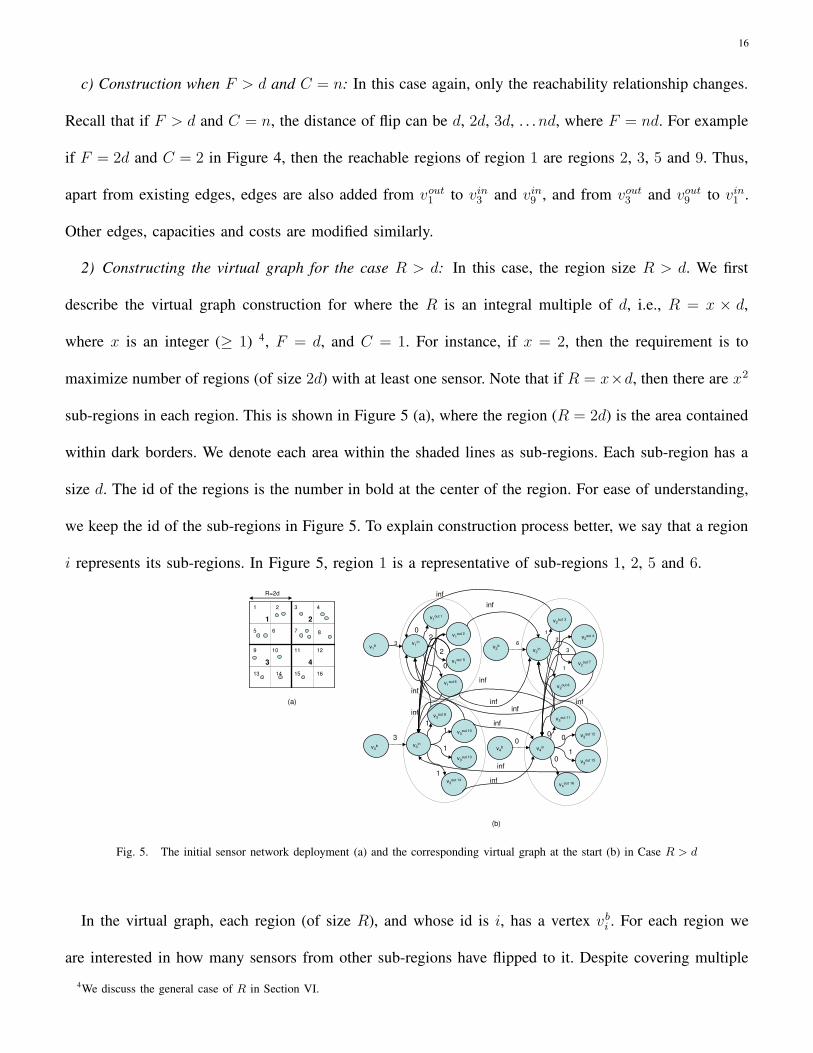
2) Constructing the virtual graph for the case R > d: In this case, the region size R > d. We first

describe the virtual graph construction for where the R is an integral multiple of d, i.e., R = x × d,

where x is an integer (≥ 1) 4, F = d, and C = 1. For instance, if x = 2, then the requirement is to

maximize number of regions (of size 2d) with at least one sensor. Note that if R = x×d, then there are x2

sub-regions in each region. This is shown in Figure 5 (a), where the region (R = 2d) is the area contained

within dark borders. We denote each area within the shaded lines as sub-regions. Each sub-region has a

size d. The id of the regions is the number in bold at the center of the region. For ease of understanding,

we keep the id of the sub-regions in Figure 5. To explain construction process better, we say that a region

i represents its sub-regions. In Figure 5, region 1 is a representative of sub-regions 1, 2, 5 and 6.

1

5 6

3 42

7

9 10 11 12

13 14 15 16

1 2

43

(a)

v3b

v1b

v1out 1

v1in

v1out 2

v1out 5

v1out 6

v2out 3

v2in

v2out 4

v2out 7

v2b

v2out 8

v3out 9

v3in

v3out 10

v3out 13

v3out 14

v3out 11

v4in

v3out 12

v3out 15

v4b

v4out 16

inf

inf

inf

inf

3

0

02

2

0

6

12

61

3

01

00

1

1

11

3

inf

inf

(b)

R=2d

inf

infinf

infinf

8

Fig. 5. The initial sensor network deployment (a) and the corresponding virtual graph at the start (b) in Case R > d

In the virtual graph, each region (of size R), and whose id is i, has a vertex vbi . For each region we

are interested in how many sensors from other sub-regions have flipped to it. Despite covering multiple

4We discuss the general case of R in Section VI.

17

sub-regions, we are interested in coverage of the region in itself (and not the sub-regions). Thus, we

still need only one in vertex (vini ) for each region. However, each region has multiple sub-regions, and

sensors in them can be pushed out. Thus the number of out vertices per region is equal to the number

of sub-regions as shown in Figure 5 (b). Note that, sensors do not need to make internal flips to other

sub-regions within a region, as there is no improvement in region coverage. Hence, there are no edges

created for internal flips within a region.

We now discuss how edges are added between vertices in GV . Each region i that has ≥ 1 (or = 1)

sensors, is a source region (or a forwarder region), and an edge is added from vbi to vin

i with edge capacity

equal∑x2

j=1nj −1 in the virtual graph, where x2 is the number of sub-regions in each region, and nj is

the number of sensors in sub-region j. For example in Figure 5, region 1 is a source, and there is an

edge with capacity∑

4

j=1nj −1 = 3 from vertex vb

1to vin

1. This ensures that, when determining the flow

from this region, at least one sensor remains. Then, edges with capacity nk are added from this vini to

each vout ki as shown in Figure 5, where vout k

i is the out vertex corresponding to sub-region k in region

i. For each hole j, we add an edge with capacity 1 from vinj vertex to vb

j , an edge of 0 capacity from vinj

to each vout kj in the virtual graph. Finally, to incorporate the reachability relationship between regions,

an edge of infinite capacity is added from vout mi to vin

j , and an edge of infinite capacity is added from

vout pj to vin

i if regions i and j are reachable from each other and sub-region m is reachable from region

j and sub-region p is reachable from region i as shown in Figure 5. The cost, that captures number of

flips between regions is 1 between the corresponding edges above. Other edges that are between regions

also have cost value 1. For each region i, the edges from vbi to vin

i , and from vini to voutk

i (for all k) do

not count towards sensor flips and have 0 cost (similar to the preceding case). We can obtain equations

for capacities and costs following from discussions in Section IV-B.1 in the preceding case. An instance

of original deployment and the corresponding virtual graph at the start are shown in Figures 5 (a) and (b)

respectively. We do not show the cost values in the virtual graph in Figure 5 (b).

The extensions to construct GV when F > d and C = 1, and when F > d and C = n for the case

18

where R > d are similar to those proposed for F > d and C = n, and F > d and C = 1 respectively for

the case where R = d. Due to space limitations, we do not describe the construction for these cases.

C. Determining the optimal movement plan from the virtual graph

Recall that the base vertex (vbi ) keeps track of the number of sensors in region i in GV . Also, the

edges going into the base vertices of holes have capacity one to allow a maximum of one sensor into

the holes. Consequently, our problem can be translated as determining flows from the base vertices of

source regions to as many base vertices of holes as possible in GV , with minimum overall cost. Let us

now discuss why this is true. From the construction rules of GV , we can see that for each feasible sensor

movement sequence in the sensor network between a source region and a hole, there is a feasible path for

a flow in GV between base vertices of the corresponding regions and vice-versa. For example, consider a

feasible sensor movement sequence from a source region (say i) to a hole (say j) through forwarder regions

k, l, . . . , m and n. We denote the path as a tuple of the form < i, k, l, . . . , m, n, j >. The feasibility of this

path means that each of regions i, k, l, . . . , m, n have at least one sensor in them, and region i has at least

two sensors. From the construction of GV , the capacities C(vbi , v

ini ),C(vin

i , vouti ),C(vout

i , vink ),C(vin

k , voutk ),

C(voutk , vin

l ), . . ., C(voutm , vin

n ), C(vinn , vout

n ), C(voutn , vin

j ), and C(vinj , vb

j) are all ≥ 1 (where C(i, j) was

defined in Section IV-B.1). Thus a flow from vbi to vb

j is feasible in GV5. The cost of this flow in is

the summation of cost of all edges in the path. Recall that the cost of edges from out to in of reachable

regions is one, and all other edges costs are zero. Consequently, the cost of the above flow in GV is

the number of times a flow occurs between out and in vertices of successive reachable regions in the

path. Clearly, this is the number of regions traversed in the sensor network (i.e., the number of flips). At

this point it is clear that if we can determine a flow plan (the actual flow among the edges) in GV that

can maximize the flow from the base vertices of source regions to as many base vertices of holes with

minimum overall cost, we can translate the flow plan as a movement plan for sensors (across the regions)

5A similar argument can show that for every feasible flow in GV , a corresponding sensor movement sequence is feasible in the sensornetwork.

19

in the sensor network that maximizes coverage and minimizes the number of sensor flips.

Determining the minimum cost maximum flow plan in a graph is a two step process. First, the maximum

flow value from sources to sinks in the graph is determined (for which there are many existing algorithms).

Second, the minimum cost flow plan (for this maximum flow) in the graph is determined (for which also

there are many existing algorithms). In our implementations, we first determine the maximum flow value

in GV from all base vertices of source regions to base vertices of hole regions using the Edmonds-Karp

algorithm [18]. We then determine the minimum cost flow plan (for the above maximum flow) in GV

using the method in [19], which is an implementation of the algorithm in [20]. For more details on the

algorithms, readers can refer to [18], [19] and [20]. The corresponding flow plan is a set of flows in all

edges in GV corresponding to the minimum cost maximum flow in GV .

Let W V denote the flow plan (a set of flows) corresponding to the minimum cost maximum flow in GV ,

where the amount of each flow is one. Each flow in W V is actually a path from the base vertex of a source

to the base vertex of a hole. The flow value is one for each flow, since only one sensor eventually moves

to a hole (from our problem definition). Consequently, the value of the maximum flow is the number of

such flows (with flow value one), which in turn is the maximum number of holes that can be covered

eventually with one sensor. Each flow wVi,j ∈ W V is a flow from the base vertex of a source vb

i to the base

vertex of a hole vbj in GV , and is of the form 〈vb

i , vini , vout

i , vink , vout

k , vinl , vout

l , . . . , voutm , vin

n , voutn , vin

j , vbj〉,

which denotes that the path of the flow is from vbi to vin

i , from vini to vout

i . . . , from vinj to vb

j . From

the construction of GV , for each such wVi,j (∈ W V ), a corresponding movement sequence in the sensor

network wSi,j can be determined, and is of the form 〈ri, rk, rl . . . rm, rn, rj〉, where ri, rk, rl . . . rm, rn, rj

correspond to regions i, k, l, . . . , m n, j in the sensor network respectively. Physically, this means that

one sensor should flip from regions i to k, k to l, . . . m to n and n to j. The sensor flip (or movement)

plan W S (set of all wSi,j) is the output of our solution.

Once the Base-station determines the flip plan, it will forward instructions to the sensors (that need to

flip). For each sensor, the Base-station can forward instructions on the reverse direction of the original path

20

of communication between the sensor and the Base-station. The forwarded packet contains the destination

of the sensor and the intended region the sensor needs to flip to. Since sensors know the regions they

reside in, they can determine the direction of the intended region (i.e., left, right, top or bottom region).

We assume that sensors are equipped with steering mechanisms (similar to the one in [10]) that allow

sensors to orient themselves in an appropriate direction prior to their flip. Theorem 1 shows that the flip

plan obtained by our solution optimizes both coverage and the number of flips.

Theorem 1: Let W Vopt be the minimum-cost maximum-flow plan in GV . Its corresponding flip plan W S

opt

will maximize coverage and minimize the number of flips (Refer to Appendix for proof).

We now discuss the time complexity of our solution. There are three phases in our solution while deter-

mining the optimal movement plan. The first is the virtual graph construction, the second is determining

the maximum flow, and the third is the execution of the minimum-cost flow algorithm. Denoting |V | and

|E| as the number of vertices and edges in the virtual graph respectively, we have |V | = O((dDRe2)(dR

de)2)

and |E| = O((dFde)(dR

de)(dD

Re2)), where dD

Re2 denotes the number of regions, dR

de2 denotes the number

of sub-regions and dFde denotes the number of reachable regions for each region. The time complexity of

the virtual graph construction is O(|V | + |E|). The time complexity for determining the maximum flow

using the implementation in [18] is O(|V ||E|2), and time complexity for determining the minimum cost

flow using the implementation in [20] is O(|V |2|E|log|V |). As such, the resulting time complexity of our

solution is O(max (|V ||E|2, |V |2|E|log|V |)). We wish to emphasize here that the above implementations

are not necessarily the fastest. For a detailed survey of other works on the maximum flow and minimum

cost problems, please refer to [21] and [22].

D. Extending our solution for multiple flips

Our solution presented above considered sensors that can flip only once. We now discuss how to extend

the above solution when a sensor can flip more than once. In this case, we only have to modify GV to

incorporate more reachable regions due to multiple flips. Let us consider the example in Figure 4 (a).

Let F = d, and let us assume that a sensor can flip to a distance d twice. For region 1 in Figure 4 (a),

21

its reachable regions now are regions 2, 3, 5, 6 and 9. Thus, edges are added from vout1

to vin2

, vin3

, vin5

,

vin6

and vin9

. The edge capacity is still infinity for all the edges. The cost of the edge from vout1

to vin2

and

vin5

is still one. However, since a sensor in region 1 needs two flips to move to regions 3, 6 and 9, the

cost of the edges from vout1

to vin3

, vin6

and vin9

is two. Correspondingly, edges are also added from vout2

,

vout3

, vout5

vout6

and vout9

to vin1

, with infinite edge capacity and appropriate edge costs. All other regions

are treated similarly in GV . The rest of the solution remains the same. It can be shown that the resulting

movement plan is optimal (the proof is straightforward from Theorem 1).

E. Alternate Approaches to Execute our Solution

Our solution requires information on the number of sensors in each region in the network. In the above,

we proposed to let a centralized Base station to collect this information and execute our solution. We now

discuss distributed approaches to execute our solution. In the first approach, sensors in the network once

again share information about the number of sensors in their regions. In the extreme case, a sensor in each

region can execute our solution independently with this information. An alternate distributed approach is

to divide the network into multiple areas. In this approach, we let each area to obtain region information

only in their area and not exchange it with other areas. A special sensor in each area can then execute our

solution independently only with this information (without global synchronization with other areas), and

determine a movement plan for sensors in its area. We call this the area-based approach. However, this

approach can only achieve local optima in each area and cannot guarantee global optima in the sensor

network. We will study performance of this approach further using simulations in Section V.

V. PERFORMANCE ANALYSIS

In the above, we proved the optimality of our solution in terms of coverage and number of flips. We

now study the sensitivity of coverage and the number of flips to flip distance under different choices (for

flip distance), initial deployment scenarios and coverage requirements. We also study performance and

overhead when our solution is executed using the area-based approach discussed in Section IV-E.

22

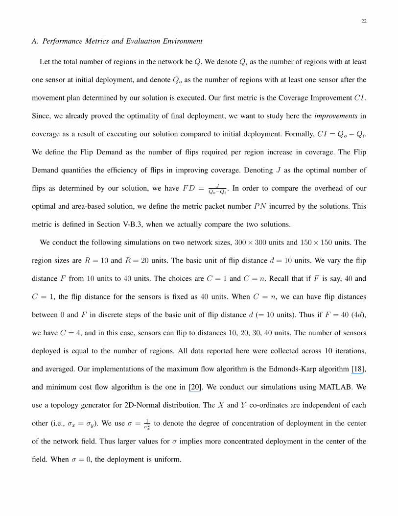
A. Performance Metrics and Evaluation Environment

Let the total number of regions in the network be Q. We denote Qi as the number of regions with at least

one sensor at initial deployment, and denote Qo as the number of regions with at least one sensor after the

movement plan determined by our solution is executed. Our first metric is the Coverage Improvement CI .

Since, we already proved the optimality of final deployment, we want to study here the improvements in

coverage as a result of executing our solution compared to initial deployment. Formally, CI = Qo − Qi.

We define the Flip Demand as the number of flips required per region increase in coverage. The Flip

Demand quantifies the efficiency of flips in improving coverage. Denoting J as the optimal number of

flips as determined by our solution, we have FD = JQo−Qi

. In order to compare the overhead of our

optimal and area-based solution, we define the metric packet number PN incurred by the solutions. This

metric is defined in Section V-B.3, when we actually compare the two solutions.

We conduct the following simulations on two network sizes, 300× 300 units and 150× 150 units. The

region sizes are R = 10 and R = 20 units. The basic unit of flip distance d = 10 units. We vary the flip

distance F from 10 units to 40 units. The choices are C = 1 and C = n. Recall that if F is say, 40 and

C = 1, the flip distance for the sensors is fixed as 40 units. When C = n, we can have flip distances

between 0 and F in discrete steps of the basic unit of flip distance d (= 10 units). Thus if F = 40 (4d),

we have C = 4, and in this case, sensors can flip to distances 10, 20, 30, 40 units. The number of sensors

deployed is equal to the number of regions. All data reported here were collected across 10 iterations,

and averaged. Our implementations of the maximum flow algorithm is the Edmonds-Karp algorithm [18],

and minimum cost flow algorithm is the one in [20]. We conduct our simulations using MATLAB. We

use a topology generator for 2D-Normal distribution. The X and Y co-ordinates are independent of each

other (i.e., σx = σy). We use σ = 1

σ2x

to denote the degree of concentration of deployment in the center

of the network field. Thus larger values for σ implies more concentrated deployment in the center of the

field. When σ = 0, the deployment is uniform.

23

0

20

40

60

80

100

120

10 20 30 40 F

CI

C=1 C=n � = 1, R=10

0

50

100

150

200

250

300

350

10 20 30 40 F

CIC=1 C=n � = 1, R=10

(a) (b)

Fig. 6. Sensitivity of CI to F under different C in 150 × 150 and300 × 300 network

0

0.5

1

1.5

2

2.5

10 20 30 40 F

FD

C=1 C=n � = 0, R=10

0

0.5

1

1.5

2

2.5

3

10 20 30 40 F

FDC=1 C=n � = 0, R=10

(a) (b)

Fig. 7. Sensitivity of FD to F under different C in 150 × 150 and300 × 300 network

B. Our Performance Results

1) Sensitivity of CI and FD to F under different C: Figures 6 (a) and (b) show the sensitivity of CI to

flip distance F under different choices C in two different network sizes (150×150 and 300×300), where

R = 10, σ = 1 and d = 10. The number of regions in the networks are 15× 15 = 225 and 30× 30 = 900

respectively. We observe that in both figures, for a given value of F , C = n has larger CI compared

to C = 1, except for F = d = 10, when both C = n and C = 1 have the same performance. This is

because, when F = 10, we have n = 1, and so C = n is the same as C = 1. However, when F > 10,

for a given F there are more flip choices that our solution can exploit when C = n, hence increasing

CI . The second observation we make is that when C = n, as F increases CI increases in both figures.

This is also because when C = n, an increase in F means more choices to exploit. However, the trend

is different when C = 1. In general, a large flip distance (even when C = 1) may appear to be perform

better as more far away holes can be filled if F increases. However, when C = 1, such improvements

depend on the size of the network. Beyond a certain point (depending on the network size), an increase

in F becomes counter-productive. This is due to two reasons. First many sensors near the borders of

the sensor network have flips that cannot be exploited when F is too large. Secondly, the chances of

sequential flips (i.e., sensor x flipping to sensor y’s region, sensor y flipping to sensor z’s region and so

on) to cover holes are reduced when F is too large. The value of F , where this shift takes place in the

150 × 150 network in Figure 6 (a) is F = 40, where CI decreases. Such a shift is not observed for the

300 × 300 network in Figure 6 (b), as the network size is quite large.

24

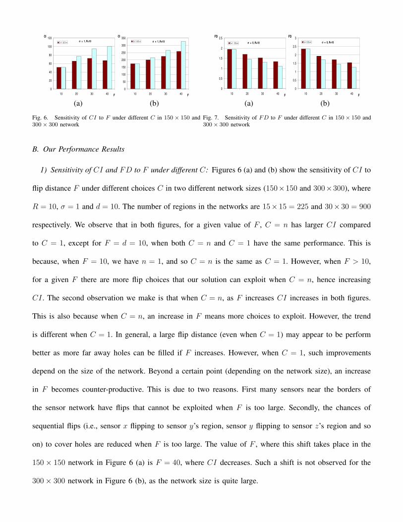
Figures 7 (a) and (b) show the sensitivity of flip demand FD to flip distance F under different choices

C in two different network sizes. We wish to emphasize here that the number of flips does not linearly

increase with coverage. Consequently, to enable a fairer comparison, we compare FD across different

cases when the final coverage is the same. For both network sizes, we set R = 10 and σ = 0, where the

final deployment covers all regions. Since the initial distribution is the same, the coverage improvement

is the same. The comparison becomes more meaningful. From Figures 7 (a) and (b), we see that for a

given value of F , C = n has a lower FD than C = 1, except for F = d = 10, when both C = n and

C = 1 have the same performance. This observation is consistent with our earlier observations on CI .

The second observation we make is that as F increases, FD decreases irrespective of C in both figures.

When F is small, in order to achieve optimality, there may be multiple flips from sensors farther away

from a hole (although the number of flips is still optimum). As F increases, it is likely that far away

sensors can flip to such holes directly, minimizing the number of flips. By comparing Figures 7 (a) and

(b), we observe that FD is more for the 300 × 300 network compared to the 150 × 150 network. For a

larger network with more regions, more flips have to be made. Consequently FD is larger.

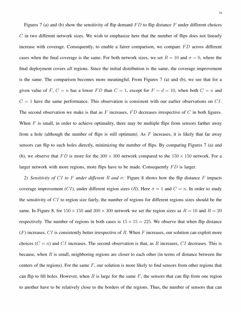
2) Sensitivity of CI to F under different R and σ: Figure 8 shows how the flip distance F impacts

coverage improvement (CI), under different region sizes (R). Here σ = 1 and C = n. In order to study

the sensitivity of CI to region size fairly, the number of regions for different regions sizes should be the

same. In Figure 8, for 150 × 150 and 300 × 300 network we set the region sizes as R = 10 and R = 20

respectively. The number of regions in both cases is 15 × 15 = 225. We observe that when flip distance

(F ) increases, CI is consistently better irrespective of R. When F increases, our solution can exploit more

choices (C = n) and CI increases. The second observation is that, as R increases, CI decreases. This is

because, when R is small, neighboring regions are closer to each other (in terms of distance between the

centers of the regions). For the same F , our solution is more likely to find sensors from other regions that

can flip to fill holes. However, when R is large for the same F , the sensors that can flip from one region

to another have to be relatively close to the borders of the regions. Thus, the number of sensors that can

25

0

20

40

60

80

100

120

10 20 30 40 F

CI

R=10 R=20 � = 1

Fig. 8. Sensitivity of CI to F under different R

0

30

60

90

120

10 20 30 40 F

CI

� = 0 � = 1� = 2

R=10

Fig. 9. Sensitivity of CI to F under different σ

be found to flip are less. Naturally CI (which captures improvement) decreases when R is large. Thus,

performance improvement due to increases in flip distance is constrained by the desired region size.

Figure 9 shows how the flip distance F impacts CI under different distributions in initial deployment.

The network size is 150× 150, R = 10, and C = n. We vary σ from 0 (uniform distribution) to 4 (highly

concentrated at the center of the field). The first observation we make here is that increases in flip distance

(F ) increases CI . However, the degree of increase in CI is impacted by σ. When σ = 0 (uniform), CI is

almost the same for all values of F . This is because, in our simulations, close to full coverage is achieved

when σ = 0. Since the initial deployment is the same for all cases, the improvement is the same.

We now study the trade-off between increasing F and σ in terms of which parameter has a more

dominating effect on CI . In Figure 9, when F = 10, σ dominates over F . We can see that as σ increases

(bias increases), CI deceases. The increase in bias cannot be compensated using sensors with flip distance

of only 10 units. However, when F increases, our solution can exploit more choices (C = n). Thus F

dominates when it increases. However, the degree of domination still depends on σ. When F = 20,

σ = 1 performs better that σ = 0. This is because, the increase in bias can be compensated better when

F = 20 (than was the case, when F = 10). Thus, CI increases. However, increasing σ beyond this point

makes the bias dominate and consequently CI decreases. When F > 20, the increase in F consistently

dominates the increase in bias (although the degree of domination is different), showing that performance

improvement due to increases in flip distance is limited by initial deployment distribution.

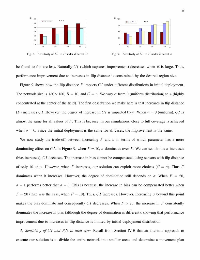
3) Sensitivity of CI and PN to area size: Recall from Section IV-E that an alternate approach to

execute our solution is to divide the entire network into smaller areas and determine a movement plan

26

0

20

40

60

80

100

15 5 3 A

CI

F=20, � = 1, R=10

100

130

160

190

220

250

30 15 10 5 A

CI

F=20, � = 1, R=10

(a) (b)

Fig. 10. Sensitivity of CI to A in 150×150 and 300×300 network

0

5

10

15

15 5 3 A

PN

F=20, � = 1, R=10

0

5

10

15

20

30 15 10 5 A

PN

F=20, � = 1, R=10

(a) (b)

Fig. 11. Sensitivity of PN to A in 150×150 and 300×300 network

in each area independently. We study this approach under two network sizes: 150 × 150 and 300 × 300.

We set R = 10, F = 20, C = n and σ = 1 for both cases. Thus, the number of regions are 225 and

900 respectively. We divide the networks into multiple areas. We denote the area size A as the number

of regions along one dimension in each area 6.

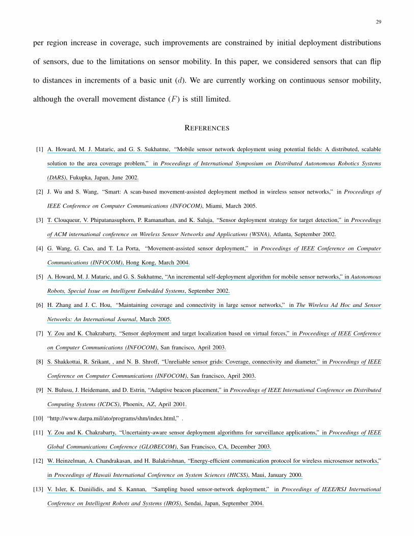
We introduce a new metric here called packet number per region PN . Denoting P as the total number

of packets (or messages) sent, and Q as the number of regions, we have PN = PQ

. The packet number

quantifies the overhead incurred by the approaches. The packet number is calculated based on a simple

protocol. After initial deployment, an elected region-head in each region sends a packet to Base-station

(located in the center of the network) with information on the number of sensors in its region. The packets

are forwarded along shortest paths through other regions. After the Base-station receives all packets and

determines a movement plan, it sends a packet to each region in the reverse path, informing sensors of

their movement plan. A similar protocol is assumed for the area-based approach, where the region-head

in each area will forward region information to a special sensor in the area, which executes the algorithm

and forwards a movement plan to each region in the area. Note that, there can be other versions of the

above protocols, like direct relaying of messages, row-wise (or column wise) message delivery etc.

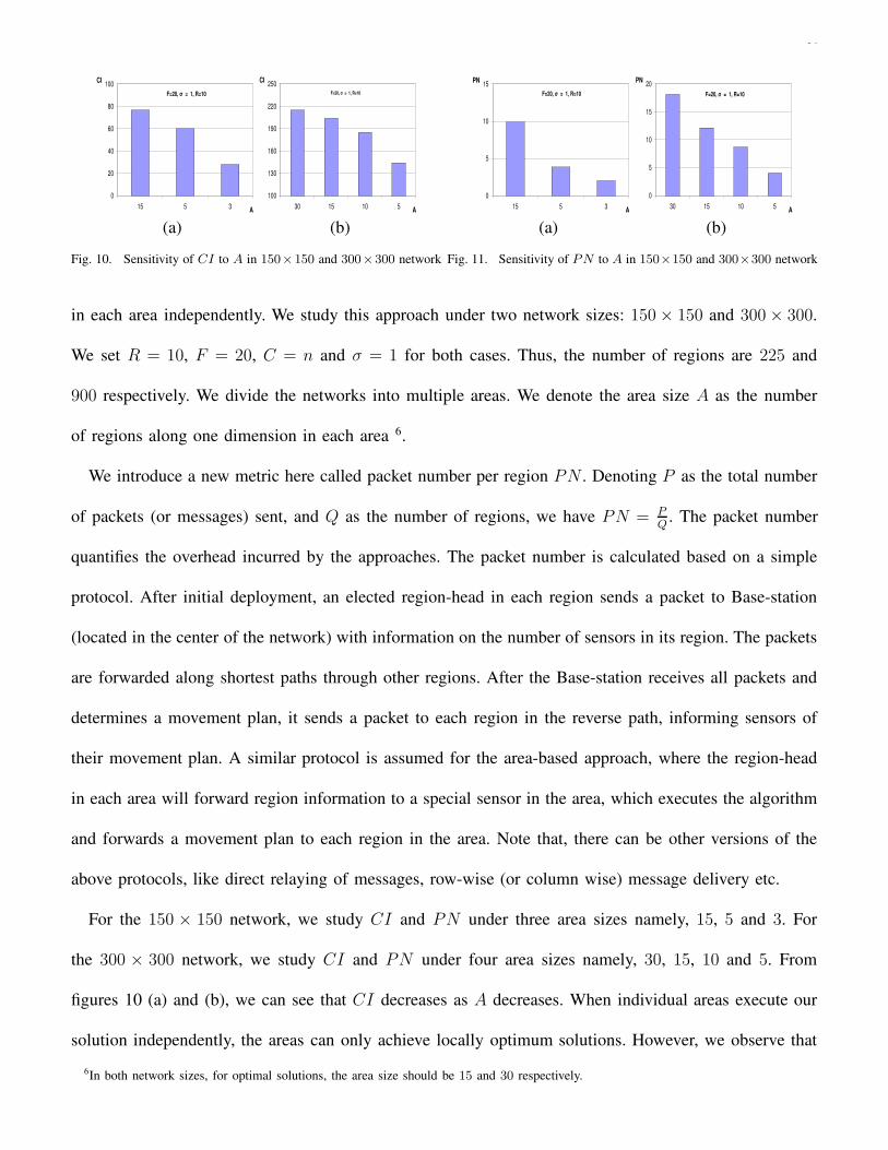
For the 150 × 150 network, we study CI and PN under three area sizes namely, 15, 5 and 3. For

the 300 × 300 network, we study CI and PN under four area sizes namely, 30, 15, 10 and 5. From

figures 10 (a) and (b), we can see that CI decreases as A decreases. When individual areas execute our

solution independently, the areas can only achieve locally optimum solutions. However, we observe that

6In both network sizes, for optimal solutions, the area size should be 15 and 30 respectively.

27

when the area size is half of the network size (i.e., A = 15 in Figure 10 (b)), CI is close to the globally

optimum case. This is because of the exploitation of the bias in initial deployment. Since sensors are

initially deployed one time targeted at the center of the network, the sensors are uniformly balanced in

all directions surrounding the center. In this case, if we choose the area size as half the network size

(resulting in four areas), we are optimizing deployment independently in the four directions from the

center of the network. Since the sensors are uniformly balanced in all the four directions, the ensuing CI

is not far from optimal (when A = 15 in Figure 10 (b)). Figures 11 (a) and (b) show the packet numbers

for the optimal algorithm and the area-based approach. We can see that PN decreases as A decreases,

demonstrating the savings in overhead in the area-based approach.

VI. DISCUSSIONS

Extensions to construct the virtual graph for any Region size R: In the above, we discussed the

construction of the virtual graph when R was an integral multiple of d. In the following, we discuss

the construction for any general value of R. Without loss of generality, let R = sd + xd, where s is an

integer (≥ 0) and x is a real number (1.0 ≥ x ≥ 0). In preceding cases, x was either 1.0 (R = (s + 1)d)

or 0 (R = sd). Let us now consider the case when (1.0 > x > 0). For two adjacent regions (say regions

i and j), we cannot determine whether a sensor in region i can flip to region j in case 1.0 > x > 0. To

circumvent this problem, we leverage the concept of sub-regions. For each region of size R, we add a

certain number of sub-regions of same size that meets the following condition; the size of each sub-region

should be a factor of d, and a factor of R. In this situation, we can correctly determine if a sensor in

a particular sub-region can or cannot flip to another region. This can be done by traversing an integral

number of sub-regions depending on d and the size of sub-regions. Our above solution is optimal if x

is a terminating decimal. If x is non-terminating (e.g. x = 1

3, 2

3etc.), we can choose an approximate

sub-region size, such that the number of sub-regions is an integral multiple of R. The smaller the size of

the sub-region, smaller is the error from optimality in this case.

Network partitions: In some situations the network may be partitioned, and we many need to repair

28

them. In the approach proposed by Wu and Wang [2], empty holes are filled by placing a seed from a

non-empty region to a hole. The algorithms to place seeds are tuned to meet load balancing objectives.

We can apply the algorithms in [2] to repair partitions in our case. Once seeds are placed, our proposed

solution can be executed. The key issue is the optimality of final coverage and the number of flips, given

the mobility limitations of sensors. Developing optimal solutions for partition recovery problem using

flip-based sensors is a part of our on-going work.

Arbitrary flip directions: Our solution can be extended to handle situations where a sensor can flip to

regions in arbitrary directions apart from left, right, top and bottom directions. The reachability relationship

between regions changes under arbitrary flip directions. In GV , we have to add edges from each region

to all newly reachable regions from it, corresponding to arbitrary directions of sensor flips.

Deployment under hostile zones/ failures in Sensor Networks: In some cases, there may be certain

hostile zones in the network (lakes, fires, etc.) that can destroy sensors. To avoid sensor flips to such

zones, we only have to modify the edges and their capacities to such hostile zones in the virtual graph.

The resulting solution is optimal.

In some cases, there can be faults/ failures in the sensors and their communication. For example, if a

sensor makes an erroneous movement to a region other than the intended region, there will be an extra

hole in the network. Or if a packet from a region does not reach the Base-station, the region will be

incorrectly treated as a hole, which may result in extra sensors in that region. As such, our solution can

tolerate a degree of faults/ failures in the network at a cost of optimality. A rigorous study of deployment

under faults/ failures will be part of future work.

VII. FINAL REMARKS

In this paper, we studied sensor network deployment using flip-based sensors. We proposed a minimum-

cost maximum-flow based solution to optimize coverage and the number of flips. We also proposed

multiple approaches to execute our solution in practice. Our performance data demonstrated that while

increased flip-distances achieves better coverage improvement, and reduces the number of flips required

29

per region increase in coverage, such improvements are constrained by initial deployment distributions

of sensors, due to the limitations on sensor mobility. In this paper, we considered sensors that can flip

to distances in increments of a basic unit (d). We are currently working on continuous sensor mobility,

although the overall movement distance (F ) is still limited.

REFERENCES

[1] A. Howard, M. J. Mataric, and G. S. Sukhatme, “Mobile sensor network deployment using potential fields: A distributed, scalable

solution to the area coverage problem,” in Proceedings of International Symposium on Distributed Autonomous Robotics Systems

(DARS), Fukupka, Japan, June 2002.

[2] J. Wu and S. Wang, “Smart: A scan-based movement-assisted deployment method in wireless sensor networks,” in Proceedings of

IEEE Conference on Computer Communications (INFOCOM), Miami, March 2005.

[3] T. Clouqueur, V. Phipatanasuphorn, P. Ramanathan, and K. Saluja, “Sensor deployment strategy for target detection,” in Proceedings

of ACM international conference on Wireless Sensor Networks and Applications (WSNA), Atlanta, September 2002.

[4] G. Wang, G. Cao, and T. La Porta, “Movement-assisted sensor deployment,” in Proceedings of IEEE Conference on Computer

Communications (INFOCOM), Hong Kong, March 2004.

[5] A. Howard, M. J. Mataric, and G. S. Sukhatme, “An incremental self-deployment algorithm for mobile sensor networks,” in Autonomous

Robots, Special Issue on Intelligent Embedded Systems, September 2002.

[6] H. Zhang and J. C. Hou, “Maintaining coverage and connectivity in large sensor networks,” in The Wireless Ad Hoc and Sensor

Networks: An International Journal, March 2005.

[7] Y. Zou and K. Chakrabarty, “Sensor deployment and target localization based on virtual forces,” in Proceedings of IEEE Conference

on Computer Communications (INFOCOM), San francisco, April 2003.

[8] S. Shakkottai, R. Srikant, , and N. B. Shroff, “Unreliable sensor grids: Coverage, connectivity and diameter,” in Proceedings of IEEE

Conference on Computer Communications (INFOCOM), San francisco, April 2003.

[9] N. Bulusu, J. Heidemann, and D. Estrin, “Adaptive beacon placement,” in Proceedings of IEEE International Conference on Distributed

Computing Systems (ICDCS), Phoenix, AZ, April 2001.

[10] “http://www.darpa.mil/ato/programs/shm/index.html,” .

[11] Y. Zou and K. Chakrabarty, “Uncertainty-aware sensor deployment algorithms for surveillance applications,” in Proceedings of IEEE

Global Communications Conference (GLOBECOM), San Francisco, CA, December 2003.

[12] W. Heinzelman, A. Chandrakasan, and H. Balakrishnan, “Energy-efficient communication protocol for wireless microsensor networks,”

in Proceedings of Hawaii International Conference on System Sciences (HICSS), Maui, January 2000.

[13] V. Isler, K. Daniilidis, and S. Kannan, “Sampling based sensor-network deployment,” in Proceedings of IEEE/RSJ International

Conference on Intelligent Robots and Systems (IROS), Sendai, Japan, September 2004.

30

[14] A. Howard, M. J. Mataric, and G. S. Sukhatme, “Relaxation on a mesh: a formation for generalized localization,” in Proceedings of

IEEE/RSJ International Conference on Intelligent Robots and Systems (IROS), Maui, November 2001.

[15] B. Karp and H.T. Kung, “Greedy perimeter stateless routing for wireless networks,” in Proceedings of ACM International Conference

on Mobile Computing and Networking (MOBICOM), Boston, August 2000.

[16] Y. Xu, J. Heidemann, and D. Estrin, “Geography-informed energy conservation for ad hoc routing,” in Proceedings of ACM International

Conference on Mobile Computing and Networking (MOBICOM), Rome, July 2001.

[17] P. Bose, P. Morin, I. Stojmenovic, and J. Urrutia, “Routing with guaranteed delivery in ad hoc wireless networks,” in Proceedings of

International Workshop on Discrete Algorithms and methods for mobile computing and communications, Seattle, August 1999.

[18] T. Cormen, C. Leiserson, R. Rivest, and C. Stein, “Introduction to algorithms,” in MIT Press, 2001.

[19] A. V. Goldberg, “An efficient implementation of a scaling minimum-cost flow algorithm,” in J. Algorithms 22, 1997.

[20] A. V. Goldberg and R. Tarjan, “Solving minimum-cost flow problems by successive approximation,” in Proceedings of ACM Symposium

on Theory of Computing (STOC), New York, May 1987.

[21] A. V. Goldberg, “Recent developments in maximum flow algorithms,” in Proceedings of Scandinavian Workshop on Algorithm Theory

(SWAT), 1998.

[22] P. T. Sokkalingam, R. K. Ahuja, and J. B. Orlin, “New polynomial-time cycle-canceling algorithms for minimum-cost flows,” in

Networks, 36, 53-63, 2000.

APPENDIX

Proof of Theorem 1 in Section IV-C

Proof: We first prove that our solution optimizes coverage. We prove by contradiction. Consider a

flip plan W Sopt in the sensor network corresponding to a flow plan W V

opt in GV obtained by our solution.

Let W Sopt be non-optimal in terms of coverage. This means there is a better flip plan, W S

x that can cover

at least one extra region in the sensor network. Clearly, a corresponding flow plan W Vx can be found in

GV . The amount of flow in W Vx is larger than the maximum flow in W V

opt. This is a contradiction.

We now prove that our solution optimizes the number of flips. We prove by contradiction. Consider a

flip plan W Sopt in the sensor network corresponding to a flow plan W V

opt in GV obtained by our solution.

Let W Sopt be non-optimal in terms of the number of flips. This means there is a better plan, W S

x that can

reduce at least one flip in the sensor network. Clearly, a corresponding flow plan W Vx can be found in

GV . The number of flips in W Vx is less than that in W V

opt. This is a contradiction.