Airport Capacity Enhancement Analysis Through Fast-Time Simulations

Lisbon’s Airport Case Study

Gustavo Lopes Craveiro

Thesis to obtain the Master of Science Degree in

Aerospace Engineering

Supervisors: Prof. Vasco Domingos Moreira Lopes Miranda dos Reis

Prof. Maria do Rosário Maurício Ribeiro Macário

Examination Committee

Chairperson: Prof. José Fernando Alves da Silva

Supervisor: Prof. Vasco Domingos Moreira Lopes Miranda dos Reis

Member of the Committee: Prof. Pedro da Graça Tavares Alvares Serrão

March 2017

i

Resumo

Neste trabalho estudaram-se novas soluções para o aumento da capacidade do aeroporto de

Lisboa utilizando o software de Fast-Time Simulations CAST Aircraft.

Inicialmente é feito um resumo teórico dos conceitos de capacidade aeroportuária e dos

métodos para aumento de capacidade da pista de um aeroporto. É também feita uma revisão de

literatura referente ao tema, nomeadamente em relação aos modelos analíticos e de simulação mais

relevantes.

De seguida é feito o estudo do aeroporto em causa. Para tal, primeiro, procedeu-se à criação

de um modelo simplificado do aeroporto atual para servir de cenário de referência. Gerou-se tráfego

de aeronaves (fictício) até alcançar uma calibração aceitável do modelo, recorrendo a dados

históricos para uma das pistas do aeroporto.

Posteriormente, com base numa recomendação feita pela EUROCONTROL em estudos

semelhantes e analisando os resultados obtidos com o cenário de referência, desenvolveram-se 3

novos cenários: estudou-se a introdução de uma nova saída para uma das pistas do aeroporto, a

adoção de novas separações temporais entre aeronaves nos segmentos de partida e a combinação

dos dois anteriores.

Analisando os resultados chegou-se à conclusão que será possível aumentar a capacidade do

aeroporto com algumas modificações no desenho de pista e, sobretudo, com separações menos

restritivas entre aeronaves no espaço aéreo terminal do aeroporto.

Palavras-Chave: Saída de Pista Rápida, Separação entre Aeronaves, Simulação Baseada em

Agentes.

ii

Abstract

In this document, new capacity enhancement alternatives were studied for Lisbon’s airport,

using the Fast-Time simulations software CAST Aircraft.

Initially, airport’s capacity concepts and factors theoretical background is presented.

Additionally, the literature regarding the topic is also reviewed, with the main focus on the most

relevant analytical and simulation models used for these purposes.

Firstly, the Lisbon’s airport case study is introduced. In order to do that, the airport’s baseline

scenario model is created. Then, traffic is generated and increased until the model is calibrated

according to historical data for one of the airport’s runways.

Then, based on EUROCONTROL’s recommendations and analyzing the baseline scenario

results, 3 new scenarios are created: study of additional exits to one of the airport’s runways, the

analysis of less-restrictive departure/departure separations and the combination of both

alternatives.

After comparing the scenarios results, it was concluded that the airport’s capacity could be

increased with small changes on the runway layout and, most important, with the introduction of

less restrictive aircraft separation in the airport’s terminal maneuvering area.

Keywords: Rapid Exit Taxiway, Departure-Departure Separations, Agent-Based Simulation.

iii

Table of Contents

Resumo ............................................................................................................................................................................... i

Abstract ............................................................................................................................................................................. ii

Table of Contents ........................................................................................................................................................ iii

List of Tables ................................................................................................................................................................... v

List of Figures .............................................................................................................................................................. vii

Glossary ............................................................................................................................................................................ ix

1 Introduction ....................................................................................................................................................... 1

Motivation ...................................................................................................................................................... 1

Objectives ....................................................................................................................................................... 3

Methodology ................................................................................................................................................. 3

Thesis Outline .............................................................................................................................................. 4

2 Airport Performance ...................................................................................................................................... 5

Airport Capacity .......................................................................................................................................... 6

2.1.1 Concepts ............................................................................................................................................... 6

2.1.2 Factors .................................................................................................................................................. 8

Capacity Enhancement .......................................................................................................................... 11

2.2.1 Separation Between Aircraft ................................................................................................... 11

2.2.2 Runway Occupancy Times ........................................................................................................ 16

2.2.3 Rapid Exit Taxiways .................................................................................................................... 19

3 Performance Assessment Modelling .................................................................................................... 24

Model Classification................................................................................................................................ 24

Analytical Models .................................................................................................................................... 26

Simulation Models ................................................................................................................................... 28

Model Selection ........................................................................................................................................ 31

4 Work Methodology ....................................................................................................................................... 33

Technical Approach ................................................................................................................................ 33

Available Data and Model Inputs ...................................................................................................... 34

4.2.1 LPPT/LIS Airport .......................................................................................................................... 34

4.2.2 Separation Requirements ......................................................................................................... 40

4.2.3 Aircraft Fleet Mix .......................................................................................................................... 40

iv

4.2.4 Exits Usage Distribution ............................................................................................................ 41

Fast-time Simulations - CAST ............................................................................................................. 42

4.3.1 Model Structure ............................................................................................................................. 42

4.3.2 Model Configuration .................................................................................................................... 43

4.3.3 Model Initialization ...................................................................................................................... 49

4.3.4 Data Logging ................................................................................................................................... 52

Output Data Evaluation ........................................................................................................................ 54

5 Case Study ........................................................................................................................................................ 57

Scenarios ..................................................................................................................................................... 57

5.1.1 LPPT_A ............................................................................................................................................... 57

5.1.2 LPPT_B ............................................................................................................................................... 62

5.1.3 LPPT_C ............................................................................................................................................... 66

5.1.4 LPPT_D............................................................................................................................................... 68

Discussion ................................................................................................................................................... 70

6 Conclusions and Further Research ....................................................................................................... 77

References ..................................................................................................................................................................... 80

Appendix ........................................................................................................................................................................ 83

A. Standard Rapid Exit Taxiway Designs .................................................................................................... 83

B. Charts related to the aerodrome ............................................................................................................... 84

B.1 LPPT Aerodrome Chart .......................................................................................................................... 84

B.2 Aprons, Taxiways and Check Locations Data .............................................................................. 85

B.3 Ground Movement Chart Arr/Dep RWY 03 .................................................................................. 89

B.4 ILS RWY 03 Approach Chart ................................................................................................................ 90

C. Simulation Data ................................................................................................................................................. 91

C.1 Aircraft Prototypes Data........................................................................................................................ 91

C.2 LPPT_A Outputs ......................................................................................................................................... 92

C.3 LPPT_B Outputs ......................................................................................................................................... 94

C.4 LPPT_C Outputs ......................................................................................................................................... 96

C.5 LPPT_D Outputs......................................................................................................................................... 98

v

List of Tables

Table 2-1 - Airport capacity factors - examples. .................................................................................... 9

Table 2-2 - Radar wake-turbulence separation minima [22]. ......................................................... 13

Table 2-3 - IFR flights non-radar time-based separation [22]. ........................................................ 14

Table 2-4 - Major concepts for reduced wake separation. ................................................................ 15

Table 2-5 - Aerodrome code number and letter [35] . ....................................................................... 21

Table 4-1 - Current taxiways serving RWY 03. ..................................................................................... 36

Table 4-2 - Summary of key statistics for RWY03 observed in ACE’s report [71]. ..................... 37

Table 4-3 - RWY 03 ROTA by aircraft group, exit and average [71]. .............................................. 38

Table 4-4 - Key departure intervals and respective durations [71]. ............................................. 38

Table 4-5 - Taxi-in and taxi-out times observed during the summer of 2015 [72].................... 39

Table 4-6 - Exits usage distribution for medium jets observed during ACE’s exercise [71]. ... 41

Table 4-7 - Maximum aircraft speeds applied in CAST. ..................................................................... 46

Table 4-8 - Maximum aircraft accelerations applied in CAST. ......................................................... 46

Table 4-9 - Vehicle interaction rules applied in CAST. ....................................................................... 46

Table 4-10 - Flow Management waypoints and respective passage restrictions. ...................... 47

Table 4-11 - Flight states and sub states [65]. ...................................................................................... 48

Table 5-1 - Scenarios overview. ............................................................................................................... 57

Table 5-2 - Arrival aircraft separation minima. .................................................................................. 58

Table 5-3 - Aircraft fleet mix used as inputs during the simulations, by flight direction. ....... 59

Table 5-4 - Exits usage distribution for LPPT_A and LPPT_B scenarios. ....................................... 59

Table 5-5 - LPPT_A descriptive statistics - 40 replications. .............................................................. 60

Table 5-6 - RWY3 ROTs per exit for LPPT_A and LPPT_c scenarios. .............................................. 60

Table 5-7 - LPPT_A Average Arrival Exit Distribution - 40 Replications Sample........................ 60

Table 5-8 - LPPT_A Aircraft Fleet Mix - 40 Replications Sample. .................................................... 60

Table 5-9 - LPPT_A Arrival/Departure Proportion - 40 Replications Sample. ............................ 61

Table 5-10 - LPPT_A Mix of Operations - 40 Replications Sample. ................................................. 61

Table 5-11 - Exits usage distribution for LPPT_B and LPPT_D scenarios. .................................... 63

Table 5-12 - RWY 03 ROTs per exit for LPPT_B and LPPT_D scenarios. ........................................ 64

Table 5-13 - LPPT_B Average Arrival Exit Distribution - 30 Replications Sample. .................... 64

Table 5-14 - LPPT_B Aircraft Fleet Mix - 30 Replications Sample. .................................................. 64

Table 5-15 - LPPT_B descriptive statistics - 30 replications. ........................................................... 65

Table 5-16 - LPPT_B Mix of Operations - 30 Replications Sample. ................................................. 65

Table 5-17 - LPPT_B Arrival/Departure Proportion - 30 Replications Sample. ......................... 65

Table 5-18 - LPPT_C Average Arrival Exit Distribution - 40 Replications Sample. .................... 66

Table 5-19 - LPPT_C Aircraft Fleet Mix - 40 Replications Sample. .................................................. 67

Table 5-20 - LPPT_C Arrival/Departure Proportion - 40 Replications Sample........................... 67

Table 5-21 - LPPT_C Mix of Operations - 40 Replications Sample. ................................................. 67

Table 5-22 - LPPT_C descriptive statistics - 40 replications. ............................................................ 67

vi

Table 5-23 - LPPT_D Average Arrival Exit Distribution - 30 Replications Sample. .................... 68

Table 5-24 - LPPT_D Aircraft Fleet Mix - 30 Replications Sample. .................................................. 68

Table 5-25 - LPPT_D Arrival/Departure Proportion - 30 Replications Sample. ......................... 69

Table 5-26 - LPPT_D Mix of Operations - 30 Replications Sample. ................................................. 69

Table 5-27 - LPPT_D descriptive statistics - 30 replications. ........................................................... 69

Table 5-28 - Ground movements duration and delay per direction for LPPT_A with 40

replications sample. ............................................................................................................................ 71

Table 5-29 - LPPT_A duration in departure queue - 40 Replications Sample. ............................ 72

Table 5-30 - LPPT_B ground movement durations for the inbound traffic. ................................. 73

Table 5-31 - LPPT_B duration in departure queue - 30 Replications Sample. ............................ 74

Table 5-32 - LPPT_C duration in departure queue - 40 Replications Sample. ............................. 75

Table 5-33 - LPPT_D duration in departure queue - 30 Replications Sample. ............................ 75

Table 5-34 - Departure queue delay comparison................................................................................ 76

Table 5-35 - Departure queue length comparison. ............................................................................. 76

Table 5-36 - RWY throughput comparison. .......................................................................................... 76

vii

List of Figures

Figure 1.1 - Lisbon’s arport layout development from 1942 to 1992 [2]. ...................................... 1

Figure 1.2 - Full 2017 summer season LPPT runway system slot availability from 8h00-9h00

AM [5]. ....................................................................................................................................................... 2

Figure 1.3 - Flowchart representing the methodology followed....................................................... 3

Figure 2.1 - Airfiel major components [6]. .............................................................................................. 6

Figure 2.2 - Ultimate and Practical Capacity concepts [12]. ............................................................... 7

Figure 2.3 - Typical single-runway operations [15]. ............................................................................ 8

Figure 2.4 - Arriva-Departure total cycle [17]. ..................................................................................... 10

Figure 2.5 - Time separation between departures [22]..................................................................... 12

Figure 2.6 - Eurocontrol’s ROTA concept [27] . .................................................................................... 16

Figure 2.7 - Eurocontrol’s ROTD concept [27] . .................................................................................... 17

Figure 2.8 - Runway occupancy times influence on runway capacity [32]................................... 18

Figure 2.9 - Three Segment method [36]. .............................................................................................. 23

Figure 3.1 - Simulation paradigms on abstraction level scale [42]. ............................................... 25

Figure 3.2 - Gilbo capacity envelope diagram [59]. ............................................................................ 30

Figure 3.3 - Böck and Hornung capacity assessment technical approach [60]. .......................... 31

Figure 3.4 - CAST Aircraft caption [65]. .................................................................................................. 32

Figure 4.1 - Testing new layout for Lisbon’s airport in CAST. .......................................................... 34

Figure 4.2 - Overview of LPPT just after take-off from runway 21 (2008). T2 already standing

but no aprons yet, and runway 17-35 closed for repairs [67]. ................................................ 35

Figure 4.3 - LPPT terminal airspace: TMA and APP sector [70]. ..................................................... 36

Figure 4.4 - Average total movements during ACE’s report observation period [71]. .............. 38

Figure 4.5 - Main delay causes at the top 10 affected arrival airports in 2015 [73]. ................. 39

Figure 4.6 - ACE’s exercise hourly aircraft fleet mix percentage of arrival by wake vortex

category [71]. ........................................................................................................................................ 40

Figure 4.7 - ACE’s exercise hourly aircraft fleet mix percentage of departure by wake vortex

category [71]. ........................................................................................................................................ 41

Figure 4.8 - Current LPPT’s CAD model (DXF). ..................................................................................... 42

Figure 4.9 - CAST Aircraft main infrastructure elements [65]. ........................................................ 42

Figure 4.10 - After DXF import axiway intersection clean up and adjustment of junction entry

bars [65]. ................................................................................................................................................ 43

Figure 4.11 - Typical CAST local and remote airport configuration [65]. ..................................... 43

Figure 4.12 - CAST PBLs [65]. .................................................................................................................... 44

Figure 4.13 - CAST Ground Controller [65]. .......................................................................................... 44

Figure 4.14 - Runway system components in CAST [65]. .................................................................. 46

Figure 4.15 - RWY03 Departure Sector. ................................................................................................. 47

Figure 4.16 - Single flight states and transition points [65]. ............................................................ 48

Figure 4.17 - Traffic generation - Progressor conditions tree. ........................................................ 51

viii

Figure 4.18 - Queue Detector frame [65]. .............................................................................................. 53

Figure 5.1 - CAST model of current LPPT layout. ................................................................................. 58

Figure 5.2 - Terminal approach and airport model overview. ........................................................ 58

Figure 5.3- LPPT_A Normal Probability Plot - 40 Replications Sample. ........................................ 59

Figure 5.4 - LPPT_A average daily movements and departure delay (hh:mm:ss) - 40

replications sample, 10-minutes steps. ......................................................................................... 61

Figure 5.5 - CAST model for LPPT’s layout with the new RET. ......................................................... 63

Figure 5.6 LPPT_B Normal Probability Plot - 30 Replications Sample. ......................................... 64

Figure 5.7 - LPPT_B average daily movements and departure delay (hh:mm:ss) - 30

replications sample, 10-minutes steps. ......................................................................................... 65

Figure 5.8 - LPPT_C Normal Probability Plot - 40 Replications Sample. ....................................... 66

Figure 5.9 - LPPT_C average daily movements and departure delay (hh:mm:ss) - 40

replications sample, 10-minutes steps. ......................................................................................... 67

Figure 5.10 - LPPT_D Normal Probability Plot - 30 Replications Sample. .................................... 68

Figure 5.11 - LPPT_D average daily movements and departure delay (hh:mm:ss) - 30

replications sample, 10-minutes steps. ......................................................................................... 69

Figure 5.12 - LPPT_A Queue Detector dwell time (mm:ss) - scatter plot - 40 replications. ..... 72

Figure 5.13 - LPPT_B Queue Detector dwell time (mm:ss) scatter plot - 30 replications. ....... 74

Figure 5.14 - LPPT_C Queue Detector dwell time (mm:ss) scatter plot - 40 replications......... 75

Figure 5.15 - LPPT_D Queue Detector dwell time (mm:ss) scatter plot - 30 replications. ....... 76

ix

Glossary

AA Arrival-Arrival aircraft sequence

ABS Agent Based Simulation

ACATS Airport Capacity Analysis Through Simulation

ACE Airport Capacity Enhancement exercise

ADA Arrival-Departure-Arrival aircraft sequence

ADS-B Automatic Dependent Surveillance-Broadcast

AFMT Arrival Flow Management Transition

AIP Airport Information Publication

APP Approach Control Position

ARC Airport Research Center GmbH

ASDE-X Airport Surface Detection Equipment, Model-X

ATC Air Traffic Control

ATCT Airport Traffic Control Towers

ATFM Air Traffic Flow Management

ATM Air Traffic Management

ATT Arrival Threshold Transition

CAMACA Commonly Agreed Methodology for Airport Capacity Assessment

CAST Comprehensive Airport Simulation Tool

CNAP Conventional Approach Procedure

CODA Central Office for Delay Analysis

CREDOS Crosswind - Reduced Separations for Departure Operations

DD Departure-Departure aircraft sequence

DES Discrete Event Simulation

DHT Departure Holding Transition

DLT Departure Line-up Transition

DXF Drawing Exchange Format

EEC EUROCONTROL Experimental Centre

FAA Federal Aviation Administration

FACM FAA Capacity Model

FRTT Flight crew Reaction Time to Take-off clearance

HERMES Heuristic Runway Movement Event Simulation

ICAO International Civil Aviation Organization

ILS Instrument Landing System

IMC Instrument Meteorological Conditions

KPA Key Performance Area

LIDAR Light Detection and Ranging Radar

x

LOS Level of Service

LUPT Line-Up Time

MAS Multi-Agent Systems

MLS Microwave Landing System

MTOM Maximum Take Off Mass

NSA Network Sector Analyzer

PBL Push-Back Location

PI Performance Indicator

ROT Runway Occupancy Time

ROTA Runway Occupancy Time of Arrival

ROTD Runway Occupancy Time of Departure

RWY Runway

SEAP Steeper Approach Procedure

SET Sector Exit Transition

SGAP Staggered Approach Procedure

SID Standard Instrument Departure

SIMMOD Airspace Simulation Model

STAR Standard Terminal Arrival Route

TAAM Total Airspace and Airport Modeler

TFG Traffic Flow Generator

TMA Terminal Maneuvering Area

TOCD Take-off Clearance for Departure

TOFT Take-off roll Time

TWR Airport Tower

VMC Visual Meteorological Conditions

1

1 Introduction

Motivation

Since the construction of the first airport, air transportation became a useful link between

countries and a fast way to travel. The number of flights and passengers have been increasing within

last decades and with it the demand for larger and better Airports [1]. The Humberto Delgado

Airport, in Lisbon, was no exception. In fact, many changes have been made since it was first

constructed and many of those changes were done for the improvement of the airport's operation

efficiency [2].

As illustrated in Figure 1.1, the optimization of the Lisbon Airport’s maneuvering area (runway

and its accesses) has been achieved by iteratively redesigning the previous configurations, as the

airport’s infrastructure expansion beyond its perimeter is highly limited by the surrounding urban

tissue. In fact, the lack of available areas for construction and the obstacles around the airport are the

major problems that limit the airport’s expansion.

Figure 1.1 - Lisbon’s arport layout development from 1942 to 1992 [2].

Humberto Delgado airport has also strong constraints in the airspace, with direct

consequences to the runway capacity system. The proximity of Sintra and Montijo air bases, and

military priority paths, introduce limitations on civil management of that space. Moreover, the need

for large investments in technology, to reduce separation between aircraft approaching, is also

another capacity limiting problem.

At the time of writing, it was predicted that Lisbon’s main airport would be able to

accommodate 267545 movements during 2016, with maximum 40 movements per hour (total of

arrivals and departures) in the morning peak hours (0700 to 0900 UTC). Eurocontrol’s forecast

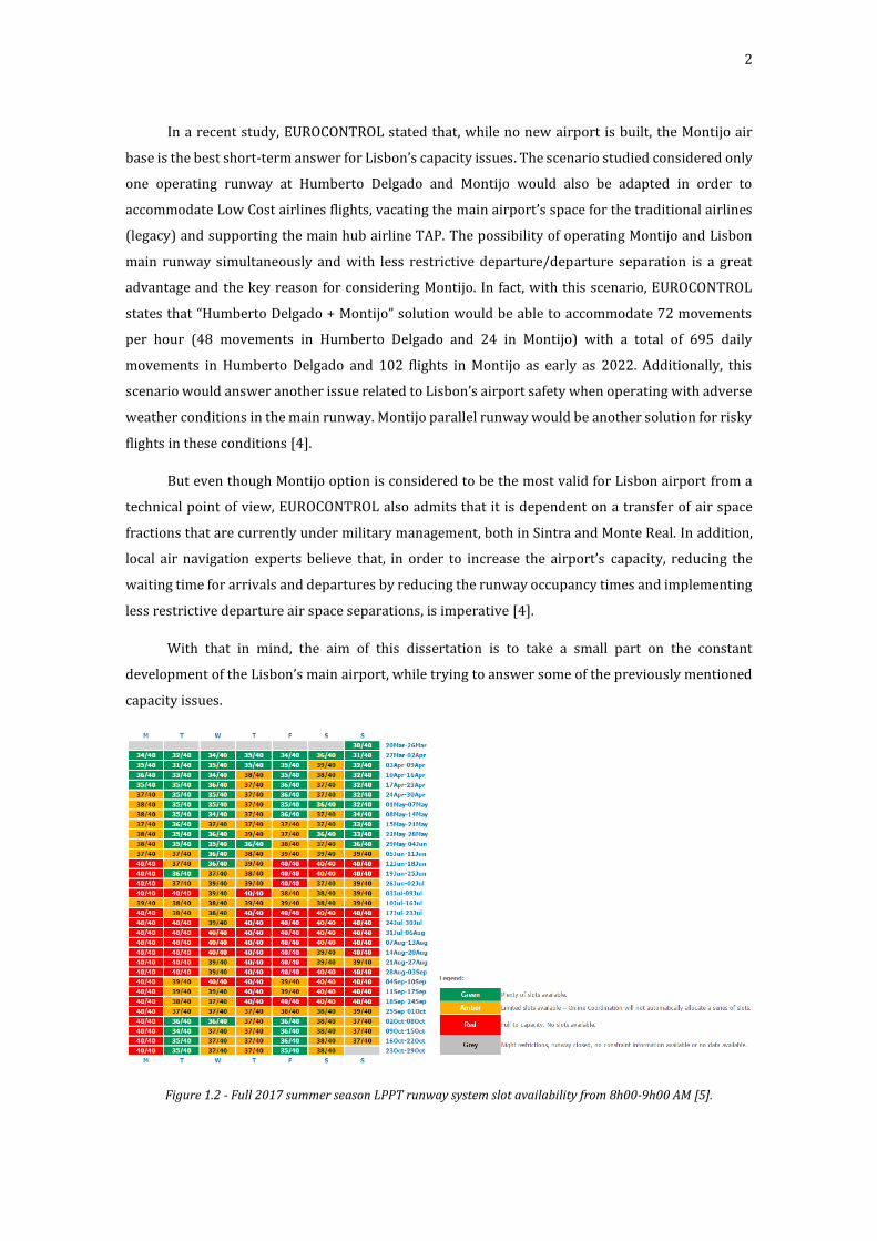
287255 movements in 2038 with the peak of 43 flights per hour [3]. As Figure 1.2 shows, in many

cases, the runway slot load is already reaching the runway system capacity limits in one of the

airport’s traffic peak hour.

2

In a recent study, EUROCONTROL stated that, while no new airport is built, the Montijo air

base is the best short-term answer for Lisbon’s capacity issues. The scenario studied considered only

one operating runway at Humberto Delgado and Montijo would also be adapted in order to

accommodate Low Cost airlines flights, vacating the main airport’s space for the traditional airlines

(legacy) and supporting the main hub airline TAP. The possibility of operating Montijo and Lisbon

main runway simultaneously and with less restrictive departure/departure separation is a great

advantage and the key reason for considering Montijo. In fact, with this scenario, EUROCONTROL

states that “Humberto Delgado + Montijo” solution would be able to accommodate 72 movements

per hour (48 movements in Humberto Delgado and 24 in Montijo) with a total of 695 daily

movements in Humberto Delgado and 102 flights in Montijo as early as 2022. Additionally, this

scenario would answer another issue related to Lisbon’s airport safety when operating with adverse

weather conditions in the main runway. Montijo parallel runway would be another solution for risky

flights in these conditions [4].

But even though Montijo option is considered to be the most valid for Lisbon airport from a

technical point of view, EUROCONTROL also admits that it is dependent on a transfer of air space

fractions that are currently under military management, both in Sintra and Monte Real. In addition,

local air navigation experts believe that, in order to increase the airport’s capacity, reducing the

waiting time for arrivals and departures by reducing the runway occupancy times and implementing

less restrictive departure air space separations, is imperative [4].

With that in mind, the aim of this dissertation is to take a small part on the constant

development of the Lisbon’s main airport, while trying to answer some of the previously mentioned

capacity issues.

Figure 1.2 - Full 2017 summer season LPPT runway system slot availability from 8h00-9h00 AM [5].

3

Objectives

The object of this dissertation is part of a current issue related to Air Traffic Management

(ATM) in Portugal: increasing Lisbon’s Airport (LPPT/LIS) traffic capacity. The main objective is to

study how some changes in the current configuration of the taxiway system and on the aircraft

separation requirements affect the Lisbon airport’s capacity through fast-time simulations.

The scope of the project was limited to the study of additional exits to one of the airport’s

runways and the analysis of less-restrictive departure/departure separations. In order to do that, a

network model representation of the airport was used to simulate the ground and airspace

movements with the help of an airport simulation software.

Methodology

Despite being a powerful analysis tool, the software used for the simulations, described in

detail next, is just part of the methodology used in this study. In fact, before starting simulating, one

should analyze the problem that is given and should obtain all the parameters that will affect the

design of new alternatives to the current airport layout and the introduction of new operational

procedures. After testing the different scenarios in respect to the runway occupancy times and

capacity, in order to study the relationship between capacity and operational efficiency, some extra

outputs need to be studied. Once better runway throughput results are obtained, if the scenario being

studied has better operational efficiency than the baseline scenario, the test can proceed and is

considered to further discussion. Usually capacity analysis considers also the estimation of delays

extent in the system as demand varies. In fact, that is a quick way of proving the viability of new

layout scenarios.

Additionally, one must derive the benefits/disadvantages of such investments before

purposing anything to the stakeholders, thus avoiding a scientific study out of real context. The

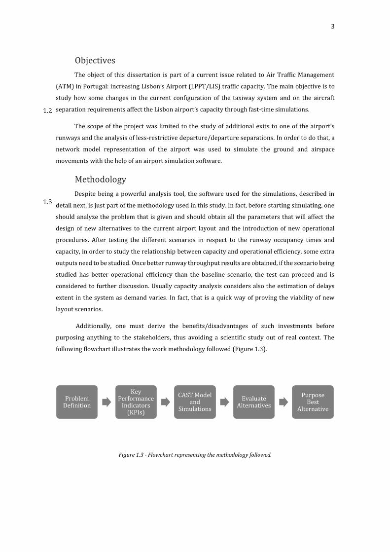
following flowchart illustrates the work methodology followed (Figure 1.3).

Figure 1.3 - Flowchart representing the methodology followed.

Problem Definition

Key Performance

Indicators (KPIs)

CAST Model and

Simulations

Evaluate Alternatives

Purpose Best

Alternative

4

Thesis Outline

This document is divided into these major chapters:

Chapter 2 - This chapter starts with a summary on the airport system basic information,

followed by information on the airport typical performance metrics, focusing on the assessment and

enhancement of the airport’s capacity.

Chapter 3 - Discusses the process of performance assessment modelling with a description of

the state of the art for analytical and simulation airport models.

Chapter 4 - Presents the methodology followed starting with the inputs for the airport’s model

and finalizing with its data logging and output analysis.

Chapter 5 – In this chapter, the reference and alternative scenarios are presented. For each

scenario, there is an overview and the simulation results are presented. After that, the different

results are compared and discussed.

Chapter 6 - Finally, in the last chapter, the conclusions of this dissertation are described, along

with future work that can be done in this matter.

5

2 Airport Performance

An airport system contains several subsystems with particular purposes and capacities that

make it possible for an aircraft to take off and land, along with many mechanisms that allow

passengers, pilots and other people involved in the operation of the airport to access the facilities on

the ground. Normally, the airport system can be divided in two main components: airspace and

airfield [6].

Airspace is defined as the portion of the atmosphere above a certain land area. This land area

can be defined in terms of the political sector that it overlays (e.g., the country or state), or it can be

defined based on proximity to the airport [7]. The airspace surrounding an airport, the so-called

Terminal Maneuvering Area (TMA), is decisive for an airport’s operational efficiency. The number of

routes that can be followed by aircraft flying into and out of the airport depends on the structure and

design of the airspace. Airspace constraints, such as high terrain, tall structures, special-use airspace,

and aircraft operations at another nearby airport, may limit the number of such routes, thereby

adversely affecting airport operation. Therefore, airspace is a very important consideration while

evaluating airport performance.

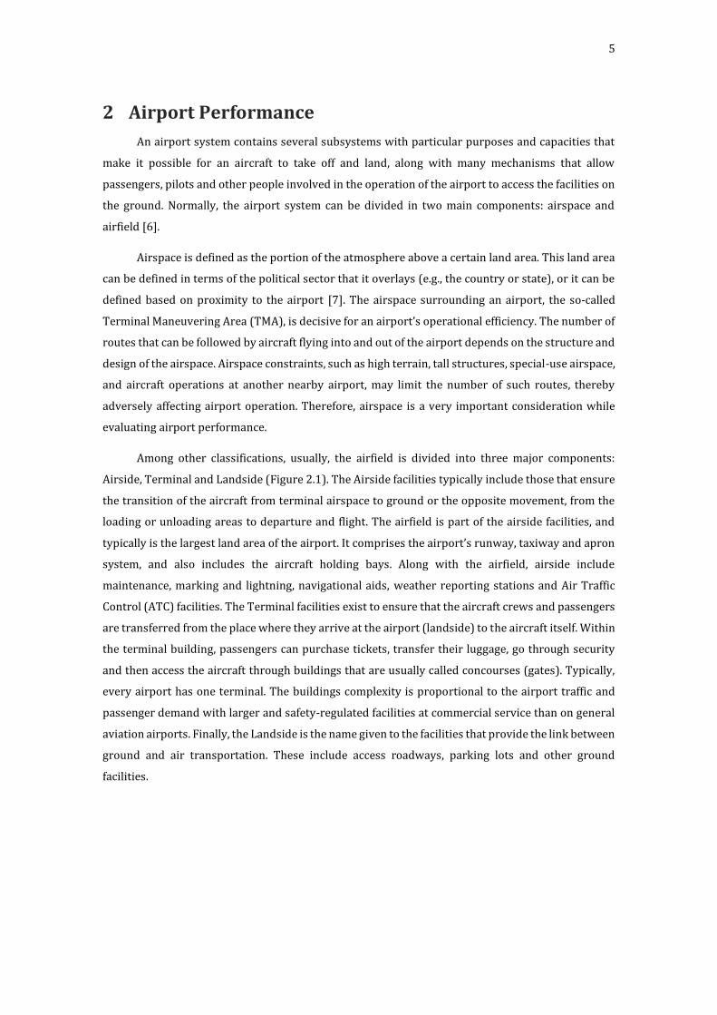
Among other classifications, usually, the airfield is divided into three major components:

Airside, Terminal and Landside (Figure 2.1). The Airside facilities typically include those that ensure

the transition of the aircraft from terminal airspace to ground or the opposite movement, from the

loading or unloading areas to departure and flight. The airfield is part of the airside facilities, and

typically is the largest land area of the airport. It comprises the airport’s runway, taxiway and apron

system, and also includes the aircraft holding bays. Along with the airfield, airside include

maintenance, marking and lightning, navigational aids, weather reporting stations and Air Traffic

Control (ATC) facilities. The Terminal facilities exist to ensure that the aircraft crews and passengers

are transferred from the place where they arrive at the airport (landside) to the aircraft itself. Within

the terminal building, passengers can purchase tickets, transfer their luggage, go through security

and then access the aircraft through buildings that are usually called concourses (gates). Typically,

every airport has one terminal. The buildings complexity is proportional to the airport traffic and

passenger demand with larger and safety-regulated facilities at commercial service than on general

aviation airports. Finally, the Landside is the name given to the facilities that provide the link between

ground and air transportation. These include access roadways, parking lots and other ground

facilities.

6

Figure 2.1 - Airfiel major components [6].

Airports operate under diverse circumstances in terms of aviation/commercial activities, site

constraints, governance and ownership structure, among others. As a result, individual airports will

find different Performance Indicators (PIs) to be most relevant and useful [8]. As recommended in

International Civil Aviation Organization’s (ICAO) Airport Economics Manual four Key Performance

Areas (KPAs) should be emphasized: safety, quality of service, productivity and cost-effectiveness

[9]. In terms of quality of service, one of the most important PI is the airport’s capacity, for example

airport average daily capacity (average aircraft movements per day) and the flight’s delay [9]. This

document will focus on the airport capacity issues, as it is the most urgent in what concerns

Humberto Delgado future.

Airport Capacity

As mentioned, airport capacity is an important performance indicator. Airport capacity

analysis serves two main functions: (a) to objectively measure the capabilities of the components of

the airport system to handle forecast aircraft movements and passenger flows and (b) to estimate

the extent of delays in the system as demand varies. Capacity can be defined as the ability of the

airport to accommodate aircraft. It is expressed as the number of operations per unit time, typically

in operations per hour [10].

2.1.1 Concepts

According to most of the relevant literature there are two basic concepts: ultimate and practical

capacity [11] [12] [10] [13] [14]. As it is explained next, the runway system is considered to be the

major capacity constraint and that is why airfield capacity is usually expressed through runway

system capacity. The definitions of ultimate and practical airport capacity by De Neufville and Odoni,

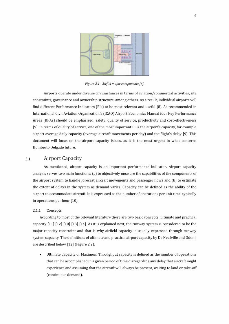
are described below [12] (Figure 2.2):

Ultimate Capacity or Maximum Throughput capacity is defined as the number of operations

that can be accomplished in a given period of time disregarding any delay that aircraft might

experience and assuming that the aircraft will always be present, waiting to land or take-off

(continuous demand).

7

Practical Capacity refers to the number of operations that can be accommodated in a given

time period, considering all constraints incumbent to the airport, and with no more than a

given amount of delay.

Figure 2.2 - Ultimate and Practical Capacity concepts [12].

There are also two concepts that are not meant for planning purposes but only for describing

reasonable capabilities of the airport systems. They are also suggested by De Neufville and Odoni:

Sustained Capacity and Declared Capacity [12]. The first one, is defined as the number of movements

that can be reasonably sustained over a period of several hours. As maximum operational

performance often cannot be guaranteed for long periods of time, Sustained Capacity is, usually, more

realistic than Ultimate Capacity. Declared capacity is defined as the number of aircraft movements

that an airport can accommodate at a reasonable Level of Service (LOS). As explained before, in the

case of air traffic, the level of service is highly related with delays so Declared Capacity can equal the

Practical Capacity in same cases.

In this document, since Lisbon’s airport is having capacity issues mainly on the major traffic

hours, Ultimate Capacity concept was found to be the most suitable for these purposes. This way, by

entering a continuous demand for both arrivals and departures flights, it is possible to study the

extreme hypothetic situation where there is always an aircraft waiting to land or to take off.

8

2.1.2 Factors

For simplicity the main features of the capacity analysis will be described for landings and

take-offs on a single runway under Instrument Flight Rules (IFR). Figure 2.3 represents a runway

with its approach and departure paths. The arrival and departure fixes may be of the order of 30-50

nautical miles from the airport while the final approach path, in line with the runway from the

approach gate to the runway threshold, may be 6-10 nautical miles long. Typically, an arriving

aircraft follows essentially a curved path from an arrival fix to the approach gate where different

paths merge. It then follows the straight glide path defined by the radar beams of the Instrument

Landing System (ILS), and touches down after passing over the threshold. After touch down the

aircraft decelerates to a speed at which it can turn off at a suitable exit. A departing aircraft travels

along the taxiways to a holding point near the runway threshold where it may have to wait before

being given clearance to line up on the runway prior to departure. After receiving take-off clearance,

the aircraft accelerates down the runway, lifts off and follows a common departure path for only a

short distance before turning towards one of a number of departure fixes.

Figure 2.3 - Typical single-runway operations [15].

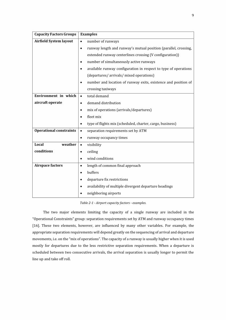
With these typical runway operations, several capacity factors can be defined and grouped

according to their nature. Table 2-1 is an example of how the factors can be distributed.

9

Capacity Factors Groups Examples

Airfield System layout number of runways

runway length and runway’s mutual position (parallel, crossing,

extended runway centerlines crossing (V configuration))

number of simultaneously active runways

available runway configuration in respect to type of operations

(departures/ arrivals/ mixed operations)

number and location of runway exits, existence and position of

crossing taxiways

Environment in which

aircraft operate

total demand

demand distribution

mix of operations (arrivals/departures)

fleet mix

type of flights mix (scheduled, charter, cargo, business)

Operational constraints separation requirements set by ATM

runway occupancy times

Local weather

conditions

visibility

ceiling

wind conditions

Airspace factors length of common final approach

buffers

departure fix restrictions

availability of multiple divergent departure headings

neighboring airports

Table 2-1 - Airport capacity factors - examples.

The two major elements limiting the capacity of a single runway are included in the

“Operational Constraints” group: separation requirements set by ATM and runway occupancy times

[16]. These two elements, however, are influenced by many other variables. For example, the

appropriate separation requirements will depend greatly on the sequencing of arrival and departure

movements, i.e. on the “mix of operations”. The capacity of a runway is usually higher when it is used

mostly for departures due to the less restrictive separation requirements. When a departure is

scheduled between two consecutive arrivals, the arrival separation is usually longer to permit the

line up and take off roll.

10

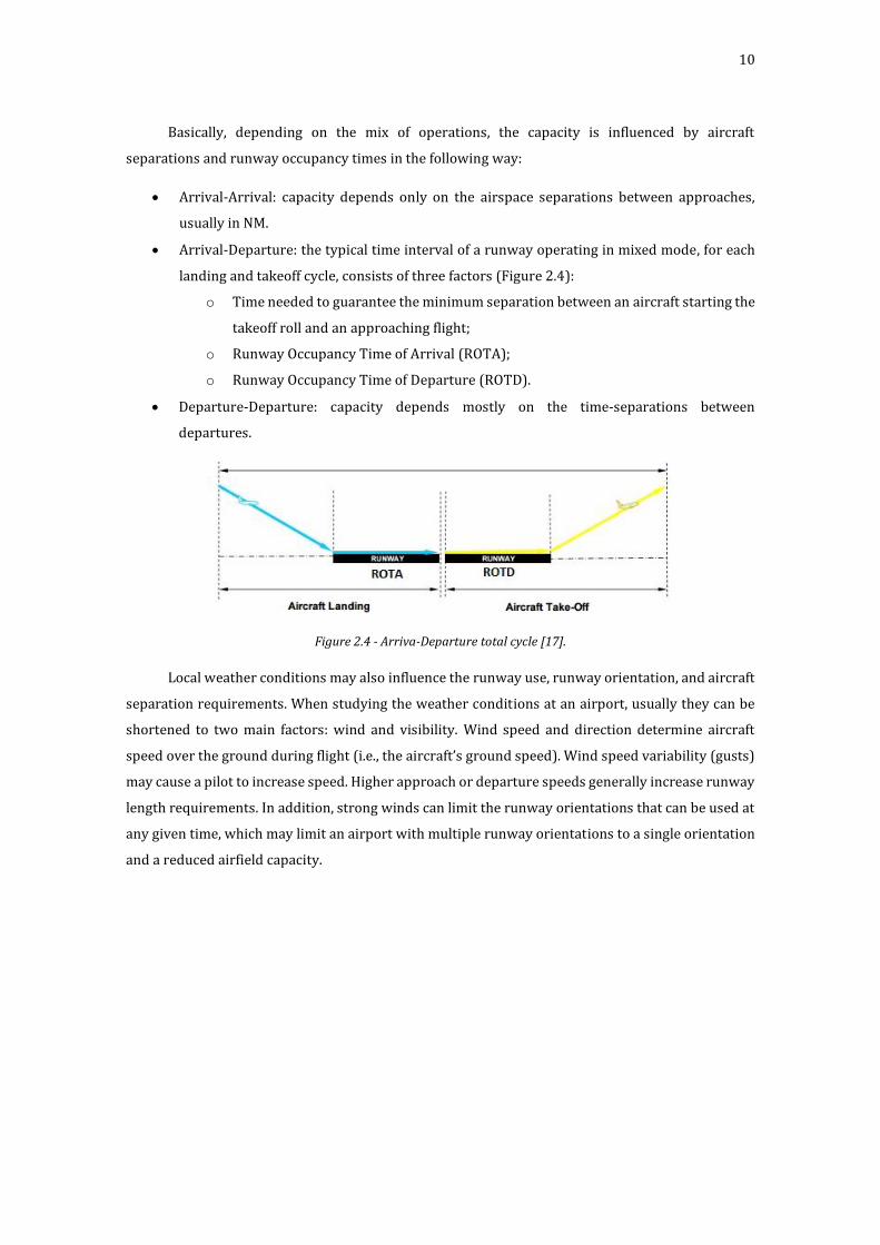
Basically, depending on the mix of operations, the capacity is influenced by aircraft

separations and runway occupancy times in the following way:

Arrival-Arrival: capacity depends only on the airspace separations between approaches,

usually in NM.

Arrival-Departure: the typical time interval of a runway operating in mixed mode, for each

landing and takeoff cycle, consists of three factors (Figure 2.4):

o Time needed to guarantee the minimum separation between an aircraft starting the

takeoff roll and an approaching flight;

o Runway Occupancy Time of Arrival (ROTA);

o Runway Occupancy Time of Departure (ROTD).

Departure-Departure: capacity depends mostly on the time-separations between

departures.

Figure 2.4 - Arriva-Departure total cycle [17].

Local weather conditions may also influence the runway use, runway orientation, and aircraft

separation requirements. When studying the weather conditions at an airport, usually they can be

shortened to two main factors: wind and visibility. Wind speed and direction determine aircraft

speed over the ground during flight (i.e., the aircraft’s ground speed). Wind speed variability (gusts)

may cause a pilot to increase speed. Higher approach or departure speeds generally increase runway

length requirements. In addition, strong winds can limit the runway orientations that can be used at

any given time, which may limit an airport with multiple runway orientations to a single orientation

and a reduced airfield capacity.

11

Cloud ceiling and visibility at the airport, which define whether aircraft are operating in Visual

Meteorological Conditions (VMC) or Instrument Meteorological Conditions (IMC), also affect airfield

capacity. Assuming all other factors are equal, fewer aircraft operations can occur when visual

approaches are not conducted, and aircraft require additional separation from one another, i.e. flights

are conducted under IFR. For example, in IMC, controllers can no longer apply visual separation from

the Airport Traffic Control Towers (ATCT) or direct pilots to conduct visual approaches to the

airport’s runways; instead, full radar separations must be applied. Moreover, increased

dependencies between runways in IMC may limit the number of simultaneous movements that can

occur at the airport. In IMC, there are stricter requirements on pilot and aircraft certifications and

performance capabilities than in VMC, which may affect the number of pilots that can fly in poor

weather conditions.

The number and types of runway exits also affect the runway occupancy and consequently the

aircraft separations. The location of the runway exits determines how long the runway is occupied

before the next landing or departure can take place on the same runway. As regulations do not allow

two aircraft occupying the same runway at the same time, that increase on the ROT will have direct

consequences on the separation between the aircraft while still on airspace and, consequently, on

the number of aircraft movements, as it is discussed next.

Capacity Enhancement

With the need to increase the capacity of airports, several approaches can be taken. One

method to increase airport capacity, more specifically the airside capacity, is to improve the capacity

of the runway system, which is a significant component of airside and where, usually, the major

bottlenecks on the airfield come from [18]. The most obvious and the single most important factor

influencing a runway system’s capacity has to do with the number of runways at the airport and their

geometric layout. By constructing a well-located (relative to the other existing runways) and well-

designed runway it is guaranteed that the capacity will increase. On the other hand, adding a new

runway requires acquisition of a large amount of additional land area with evident economic

complications since it is a great infrastructural investment. Just as important, the construction of new

runways has various environmental and other similar impacts with uncertain outcomes and

regulations problems. For these reasons, many authors have been studying the increase of the

airport’s capacity, by using existing runways more efficiently, for many years. As expected, the main

focus of runway capacity enhancement studies has been on the two major capacity limiting factors

mentioned before: minimization of aircraft separations and runway occupancy times.

2.2.1 Separation Between Aircraft

Several studies were made on the separation between aircraft during the departure and

landing phases of flight. In fact, there have been constant opportunities for improvement in this case

and, at the time of writing, there are still some relevant studies being made on this matter [19] [16]

[20] [21]. But first, it is important to clarify some basic information about aircraft separation.

12

The most obvious reason for separating aircraft is to prevent collisions. For arriving aircraft

ICAO states that: “A landing aircraft will not normally be permitted to cross the runway threshold on

its final approach until the preceding departing aircraft has crossed the end of the runway-in-use, or

has started a turn, or until all preceding landing aircraft are clear of the runway-in-use’’ [22]. For

departing aircraft, ICAO states that: ‘’A departing aircraft will not normally be permitted to

commence take-off until the preceding departing aircraft has crossed the end of the runway-in-use

or has started a turn or until all preceding landing aircraft are clear of the runway-in-use’’ [22]. But

the runway separation minima between aircraft using the same runway may be reduced in certain

situations, as described in ICAO Doc 4444 chapter 7.11 [22]. This means that the airport may reduce,

according to its needs, the ‘collision avoidance separation’ in certain situations, such as visual

separation. That is a typical capacity enhancement procedure.

When Air Traffic Control (ATC) separates the IFR flight from other flights with the aid of radar

(or ADS-B), ICAO prescribes a minimum horizontal (longitudinal) separation of 5.0 nautical miles

(9.3 km). This may be reduced at the discretion of the appropriate Air Traffic Services (ATS) authority

to 3 nautical miles (5.6 km) or even 2.5 nautical miles (4.6 km) when the conditions described in

ICAO Doc 4444 chapter 8.7.3.2b are met [22]. For departures, one-minute separation is required if

aircraft are to fly on tracks diverging by at least 45 degrees immediately after take-off so that lateral

separation is provided. Two minutes are required between take-offs when the preceding aircraft is

74km/h (40kt) or faster than the following aircraft and both will follow the same track [22](Figure

2.5).

Figure 2.5 - Time separation between departures [22].

13

Another reason to separate aircraft is wake vortex turbulence. Wake vortex turbulence is

generated from the point when the nose landing gear of an aircraft leaves the ground on take-off and

will cease to be generated when the nose landing gear touches the ground during landing [23].

According to ICAO, wake turbulence may cause three dangerous effects: induced roll, loss of height

and rate of climb and structural stress [24]. This way, wake turbulence is a serious thing to avoid by

providing enough separation between aircraft. This will have direct effects on the separation

requirements as the heavier aircraft will need a larger separation for the following aircraft. At first,

ICAO wake turbulence separations were based on certificated Maximum Take Off Mass (MTOM) and

they included three categories (i.e Heavy, Medium or Light) allocating all aircraft into one of them.

Then Airbus made the A380 model, with a maximum take-off mass of approximately 560,000 kg.

After conducting investigations and writing state letters, ICAO created a guideline in 2008

recommending a new category [25]. Because the vortices generated by the A380 are more substantial

than those of other aircraft in the Heavy wake turbulence category, a super category was introduced

for A380 aircraft (Table 2-2). These minimum separations apply whenever:

an aircraft directly follows another at the same altitude or less than 1000 ft below it;

if both aircraft are using the same runway or parallel runways separated by less than 760 m;

an aircraft is crossing behind another aircraft, at the same altitude or less than 300 m below.

Follower

A380-800 Heavy Medium Light

Lea

der

A380-800 6 NM 7 NM 8 NM

Heavy (MTOM≥136 tons) 4 NM 5 NM 6 NM

Medium (7 tons≤MTOM≤136 tons) 5 NM

Light (MTOM≤7tons)

Table 2-2 - Radar wake-turbulence separation minima [22].

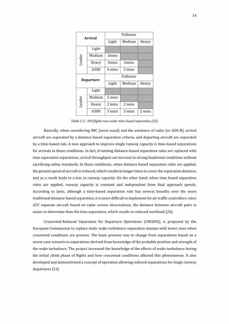
According to ICAO, when the aerodrome controller uses non-radar separation, an IFR

arrival/departure must be separated from other aircraft with time-based wake turbulence

separation. The rules applied for arriving and departing aircraft are listed in Table 2-3. One exception

applies for departures from intermediate parts of the same runway. Then, a minimum separation of

3 minutes is needed for a configuration with Light, Medium and Heavy aircraft. A separation

minimum of 4 minutes should be applied for a Light or Medium aircraft when taking off behind an

A380-800 aircraft.

14

Arrival Follower

Light Medium Heavy

Lea

der

Light

Medium 3mins

Heavy 3mins 2mins

A380 4 mins 3 mins

Departure Follower

Light Medium Heavy L

ead

er

Light

Medium 2 mins

Heavy 2 mins 2 mins

A380 3 mins 3 mins 2 mins

Table 2-3 - IFR flights non-radar time-based separation [22].

Basically, when considering IMC (most usual) and the existence of radar (or ADS-B), arrival

aircraft are separated by a distance based separation criteria, and departing aircraft are separated

by a time-based rule. A new approach to improve single runway capacity is time-based separations

for arrivals in those conditions. In fact, if existing distance-based separation rules are replaced with

time equivalent separations, arrival throughput can increase in strong headwind conditions without

sacrificing safety standards. In these conditions, when distance based separation rules are applied,

the ground speed of aircraft is reduced, which results in longer times to cover the separation distance,

and as a result leads to a loss in runway capacity. On the other hand, when time based separation

rules are applied, runway capacity is constant and independent from final approach speeds.

According to Janic, although a time-based separation rule has several benefits over the more

traditional distance-based separation, it is more difficult to implement for air traffic controllers: since

ATC separate aircraft based on radar screen observations, the distance between aircraft pairs is

easier to determine than the time separation, which results in reduced workload [26].

Crosswind-Reduced Separation for Departure Operations (CREDOS), is proposed by the

European Commission to replace static wake turbulence separation minima with lower ones when

crosswind conditions are present. The basic premise was to change from separations based on a

worst-case scenario to separations derived from knowledge of the probable position and strength of

the wake turbulence. The project increased the knowledge of the effects of wake turbulence during

the initial climb phase of flights and how crosswind conditions affected this phenomenon. It also

developed and demonstrated a concept of operation allowing reduced separations for single runway

departures [21].

15

CREDOS ended in 2009 giving way to other projects such as RECAT-EU. During recent years,

knowledge about wake vortex behavior in the operational environment has increased thanks to

measured data and improved understanding of physical processes. It was possible to revise ICAO’s

wake turbulence categorization and corresponding separation minima. The RECAT-EU program

basically splits the Heavy and Medium ICAO category into an upper and lower subcategory, using

information from the Light Detection and Ranging Radar (LIDAR) and X-band RADAR systemsTable

2-1 [20]. According to Eurocontrol, ATS can immediately expect benefits from the deployment of this

program. They specifically mention the following benefits [20]:

The runway throughput benefits can reach 5% or more during peak periods depending on

individual airport traffic mix.

For an equivalent throughput, RECAT-EU also allows a reduction of the overall flight time

for an arrival or departure sequence of traffic, and this is beneficial to the whole traffic

sequence. This may offer more flexibility for the air traffic controllers to manage the traffic.

More rapid recovery from adverse conditions, helping to reduce the overall delay and will

also enable improvements in Air Traffic Flow Management (ATFM) slot compliance through

the flexibility afforded by reduced departure separations.

The gain in capacity could even increase further by 2020 due to evolution of traffic mix: the

benefits are expected to further increase over time as the overall fleet mix is forecasted to

evolve towards larger aircraft.

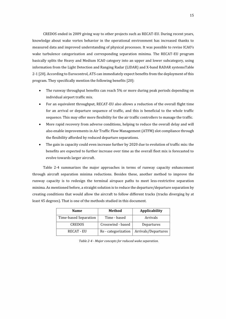
Table 2-4 summarizes the major approaches in terms of runway capacity enhancement

through aircraft separation minima reductions. Besides these, another method to improve the

runway capacity is to redesign the terminal airspace paths to meet less-restrictive separation

minima. As mentioned before, a straight solution is to reduce the departure/departure separation by

creating conditions that would allow the aircraft to follow different tracks (tracks diverging by at

least 45 degrees). That is one of the methods studied in this document.

Name Method Applicability

Time-based Separation Time - based Arrivals

CREDOS Crosswind - based Departures

RECAT - EU Re - categorization Arrivals/Departures

Table 2-4 - Major concepts for reduced wake separation.

16

2.2.2 Runway Occupancy Times

2.2.2.1 Definitions

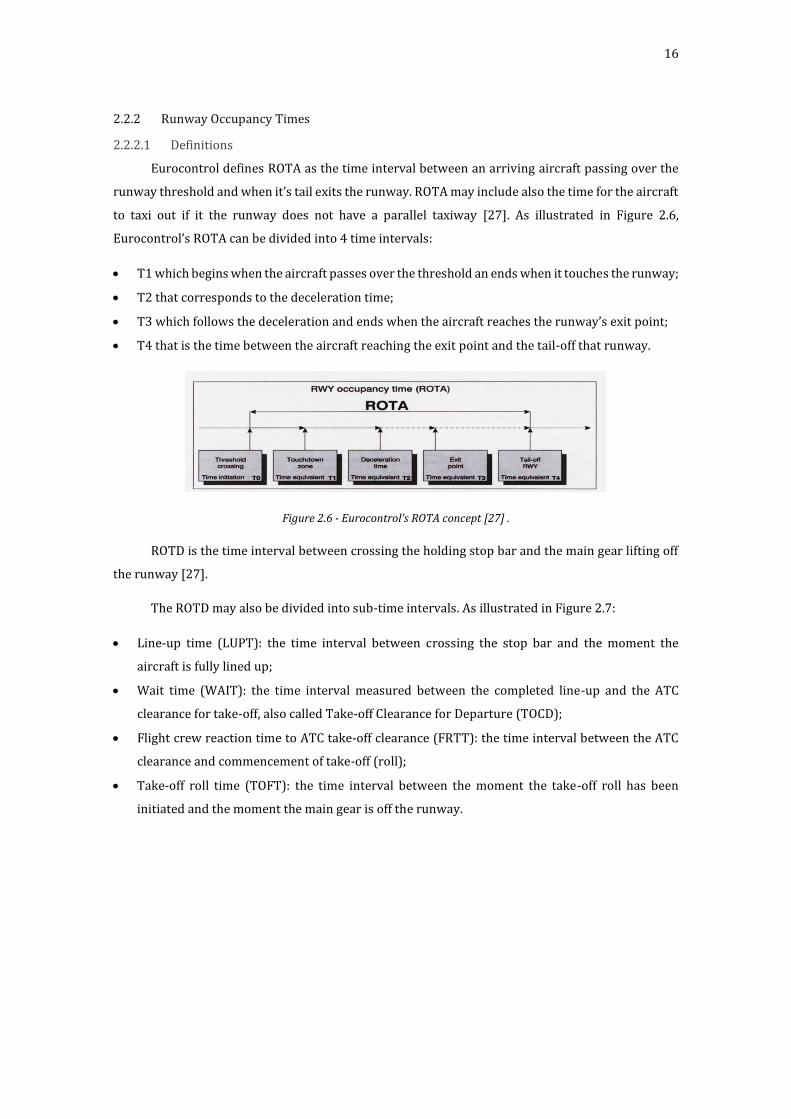
Eurocontrol defines ROTA as the time interval between an arriving aircraft passing over the

runway threshold and when it’s tail exits the runway. ROTA may include also the time for the aircraft

to taxi out if it the runway does not have a parallel taxiway [27]. As illustrated in Figure 2.6,

Eurocontrol’s ROTA can be divided into 4 time intervals:

T1 which begins when the aircraft passes over the threshold an ends when it touches the runway;

T2 that corresponds to the deceleration time;

T3 which follows the deceleration and ends when the aircraft reaches the runway’s exit point;

T4 that is the time between the aircraft reaching the exit point and the tail-off that runway.

Figure 2.6 - Eurocontrol’s ROTA concept [27] .

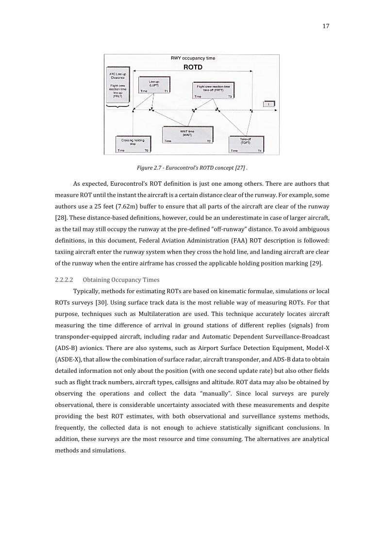
ROTD is the time interval between crossing the holding stop bar and the main gear lifting off

the runway [27].

The ROTD may also be divided into sub-time intervals. As illustrated in Figure 2.7:

Line-up time (LUPT): the time interval between crossing the stop bar and the moment the

aircraft is fully lined up;

Wait time (WAIT): the time interval measured between the completed line-up and the ATC

clearance for take-off, also called Take-off Clearance for Departure (TOCD);

Flight crew reaction time to ATC take-off clearance (FRTT): the time interval between the ATC

clearance and commencement of take-off (roll);

Take-off roll time (TOFT): the time interval between the moment the take-off roll has been

initiated and the moment the main gear is off the runway.

17

Figure 2.7 - Eurocontrol’s ROTD concept [27] .

As expected, Eurocontrol’s ROT definition is just one among others. There are authors that

measure ROT until the instant the aircraft is a certain distance clear of the runway. For example, some

authors use a 25 feet (7.62m) buffer to ensure that all parts of the aircraft are clear of the runway

[28]. These distance-based definitions, however, could be an underestimate in case of larger aircraft,

as the tail may still occupy the runway at the pre-defined “off-runway” distance. To avoid ambiguous

definitions, in this document, Federal Aviation Administration (FAA) ROT description is followed:

taxiing aircraft enter the runway system when they cross the hold line, and landing aircraft are clear

of the runway when the entire airframe has crossed the applicable holding position marking [29].

2.2.2.2 Obtaining Occupancy Times

Typically, methods for estimating ROTs are based on kinematic formulae, simulations or local

ROTs surveys [30]. Using surface track data is the most reliable way of measuring ROTs. For that

purpose, techniques such as Multilateration are used. This technique accurately locates aircraft

measuring the time difference of arrival in ground stations of different replies (signals) from

transponder-equipped aircraft, including radar and Automatic Dependent Surveillance-Broadcast

(ADS-B) avionics. There are also systems, such as Airport Surface Detection Equipment, Model-X

(ASDE-X), that allow the combination of surface radar, aircraft transponder, and ADS-B data to obtain

detailed information not only about the position (with one second update rate) but also other fields

such as flight track numbers, aircraft types, callsigns and altitude. ROT data may also be obtained by

observing the operations and collect the data “manually”. Since local surveys are purely

observational, there is considerable uncertainty associated with these measurements and despite

providing the best ROT estimates, with both observational and surveillance systems methods,

frequently, the collected data is not enough to achieve statistically significant conclusions. In

addition, these surveys are the most resource and time consuming. The alternatives are analytical

methods and simulations.

18

Analytical models are simple and provide ready application. On the other hand, their

assumptions usually are not realistic and they do not consider deviations. As mentioned above, a

popular analytical method is to assume a constant deceleration profile and use kinematic formulas

to obtain the desired ROT. Assuming average performance for the aircraft will have obvious issues

as actual ROTs show a great dispersion due to pilot and controllers action variation and also due to

the variability of weather conditions, pavement conditions, and so on.

In the case of simulation models, despite being less reliable than local surveys, the

introduction of stochastic models improves the model realistically and will allow, as long as main

inputs are available, the study of current and what-if scenarios with minor costs. Despite some

parameters in the "real world" are usually decided on a case by case basis by the pilots, as long as

there is a calibration with actual data, the use of constant values for input data, such as deceleration

and turn-off speeds, is a sensible and practical way for estimation of ROTs. That is the case of Runway

Exit Design Interactive Model (REDIM v2.1) a simulation model carried out for the FAA, and the case

of the model used in this document.

2.2.2.3 Runway Occupancy Time as element of runway capacity

ROTs are one of the most important operational factors since they are used as input/output

for several capacity models [7]. Their importance is more evident if one considers an aircraft that

occupies the runway for just a few additional seconds after arriving or during the departure, and

realize the inevitable domino effect on the rest of the airfield system capacity (Figure 2.8). Recent

studies have shown that, depending on the traffic mix, runway capacity can be increased between

5% (in the case of single-runway airports) and 15 % (multiple-runway airports) by reducing ROTs

[31]. In some cases, saving 5 seconds per movement could increase capacity by 1 to 1.5 movements

an hour [27]. With this being said, the tradeoff between the operational efficiency and the safety

issues should not be slighted. When thinking of minimizing the ROTs, the context of the study and

the implications of some changes on the current operations and (or) on the layout itself, should not

be neglected.

Figure 2.8 - Runway occupancy times influence on runway capacity [32].

19

Runway exits, aircraft and pilot performance all play an important role in controlling runway

occupancy. Stanislav et al concluded that, despite being a function of aircraft type, landing weight,

threshold speed, weather and runway conditions, the point at which the aircraft exits the runway is

largely dependent upon pilot operation techniques. They state that the pilot’s objective should be to

consistently achieve minimum runway occupancy - within the normally accepted landing and

braking performance of the aircraft - by targeting the earliest suitable exit point and applying the

right deceleration rate so that the aircraft leaves the runway as expeditiously as possible at the

nominated exit. They concluded that pilots can improve runway occupancy performance by aiming

for an exit which can be made comfortably, rather than simply aiming for an earlier exit, and rolling

slowly to the next if they miss it [31]. Those “comfortable exits” have been studied and are still a quick

way of dealing with capacity issues. In fact, throughout the years, either probabilistic models,

describing the landing of aircraft, or simulation models, were developed to evaluate the benefits from

the use of high-speed exits [33] [34]. Next, those types of exits are reviewed.

2.2.3 Rapid Exit Taxiways

The taxiway system should be designed to operate at the highest levels of both safety and

efficiency, i.e. minimize the restriction of aircraft movement to and from the runways and apron

areas, accommodating (without significant delay) the demands of aircraft arrivals and departures on

the runway system. A properly designed system should maintain a smooth, continuous flow of

aircraft ground traffic at the maximum practical speed with a minimum of acceleration or

deceleration. The taxiway system can accomplish this with a minimum number of components when

considering low levels of runway utilization. However, as the runway utilization demand increases,

the taxiway system capacity must be sufficiently expanded to avoid becoming a factor which limits

aerodrome capacity. In the extreme case of runway capacity saturation, when aircraft are arriving

and departing at the minimum separation distances, the taxiway system should allow aircraft to exit

the runway as soon as practical after landing and to enter the runway just before take-off, i.e. the ROT

should be as low as possible.

For the above-mentioned reasons, there should be a sufficient number of entrance and exit

taxiways serving a specific runway to accommodate the current demand peaks for take-offs and

landings. Additional entrances and exits should be designed and developed ahead of expected growth

in runway utilization. ICAO presents several principles to be considered while planning the layout of

these taxiway system. Quoting: “an exit taxiway can be either at a right angle to the runway or at an

acute angle. The former type requires an aircraft to decelerate to a very low speed before turning off

the runway, whereas the latter type allows aircraft to exit the runway at higher speeds, thus reducing

the time required on the runway and increasing the runway capacity” [35]. Typically, the later type

is also called Rapid Exit Taxiway (RET) and the main purpose of these taxiways is to minimize aircraft

runway occupancy and thus increase aerodrome capacity. Although the construction costs of high-

speed exits are higher than the cost of conventional exits, the additional cost may be justified if lower

runway occupancy allows for reduced separations and increased runway throughput.

20

According to ICAO, the number of exit taxiways will depend on the types of aircraft and

number of each type that operate during the peak period and the following basic planning criteria

should beconsidered when planning rapid exit taxiways to ensure that, wherever possible, standard

design methods and configurations are used [36]:

a) For runways exclusively intended for landings, a RET should be provided only if dictated by

the need for reduced runway occupancy times consistent with minimum inter-arrival

spacings;

b) For runways where alternating landings and departures are conducted, time separation

between the landing aircraft and the following departing aircraft is the main factor limiting

runway capacity;

c) As different types of aircraft require different locations for RETs, the expected aircraft fleet

mix will be an essential criterion;

d) The threshold speed, braking ability and operational turn-off speed (𝑉𝑒𝑥) of the aircraft will

determine the location of the exits.

Next, the standard geometric designs for RETs are presented and the different approaches for

finding the optimal location for those types of exits are also analyzed.

2.2.3.1 Standard Geometric Design

For the purpose of exit taxiway design, ICAO assumes that aircraft cross the threshold at an

average of 1.3 times the stall speed in the landing configuration at maximum certificated landing

mass with an average gross landing mass of about 85 per cent of the maximum. Aircraft are grouped

according to their threshold speed at sea level, in the following way [35]:

Group A: less than 169 km/h (91 kt)

Group B: between 169 km/h (91 kt) and 222 km/h (120 kt)

Group C: between 224 km/h (121 kt) and 259 km/h (140 kt)

Group D: between 261 km/h (141 kt) and 306 km/h (165 kt).

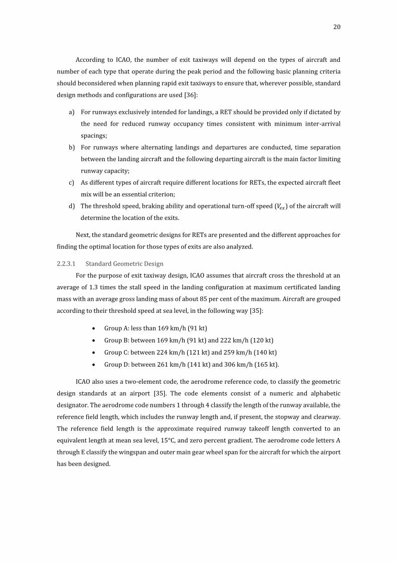
ICAO also uses a two-element code, the aerodrome reference code, to classify the geometric

design standards at an airport [35]. The code elements consist of a numeric and alphabetic

designator. The aerodrome code numbers 1 through 4 classify the length of the runway available, the

reference field length, which includes the runway length and, if present, the stopway and clearway.

The reference field length is the approximate required runway takeoff length converted to an

equivalent length at mean sea level, 15°C, and zero percent gradient. The aerodrome code letters A

through E classify the wingspan and outer main gear wheel span for the aircraft for which the airport

has been designed.

21

Aerodrome Code Number

Reference Field Length (m)

Aerodrome Code Letter

Wingspan (m)

Distance between outside edges of main

wheel gear (m) 1 <800 A <15 <4.5

2 800≤1200 B 15≤24 4.5≤6

3 1200≤1800 C 24≤36 6≤9

4 ≥1800 D 36≤52 9≤14

E 52≤65 9≤14

F 65≤80 14≤16

Table 2-5 - Aerodrome code number and letter [35] .

Annex A illustrates standard designs for rapid exit taxiways in accordance with the

specifications given in ICAO Aerodrome Design Manual [36]. Assuming deceleration rates of

0.76 𝑚/s2 along the turn-off curve, a standard rapid exit taxiway should:

be designed with radius of turn-off curve of at least 550 m where the code number is 3 or 4,

and 275 m where the code number is 1 or 2;

enable exit speeds under wet conditions of: 93 km/h (50 kt) where the code number is 3 or

4, and 65 km/h (35 kt) where the code number is 1 or 2.

It is also recommended a straight tangent section after the turnoff curve to allow exiting

aircraft to come to a full stop clear of the intersecting taxiway when the intersection is 30°. Assuming

deceleration rates of 1.52 𝑚/s2 along the straight section, this tangent distance should be:

35 m (115 ft) for aerodrome code number 1 and 2 runways and

75 m (250 ft) for aerodrome code number 3 and 4 runways.

2.2.3.2 Optimal Location

Several mathematical analyses or models have been developed for optimizing exit locations

[37] [33] . While these analyses have been useful in providing an understanding of the significant

parameters affecting location, their usefulness to planners has been limited because of the

complexity of the analyses and a lack of knowledge of the inputs required for the application of the

models. As a result, greater use is made of much more simplified methods. Using ICAO’s Three

Segment Method, it is possible to calculate the total distance required from the landing threshold to

the point of turn-off from the runway center line [36].

22

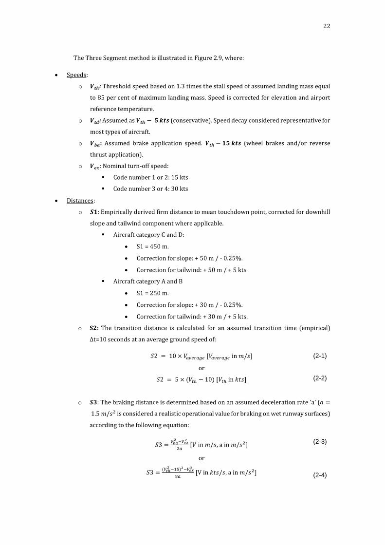
The Three Segment method is illustrated in Figure 2.9, where:

Speeds:

o 𝑽𝒕𝒉: Threshold speed based on 1.3 times the stall speed of assumed landing mass equal

to 85 per cent of maximum landing mass. Speed is corrected for elevation and airport

reference temperature.

o 𝑽𝒕𝒅: Assumed as 𝑽𝒕𝒉 − 𝟓 𝒌𝒕𝒔 (conservative). Speed decay considered representative for

most types of aircraft.

o 𝑽𝒃𝒂: Assumed brake application speed. 𝑽𝒕𝒉 − 𝟏𝟓 𝒌𝒕𝒔 (wheel brakes and/or reverse

thrust application).

o 𝑽𝒆𝒙: Nominal turn-off speed:

Code number 1 or 2: 15 kts

Code number 3 or 4: 30 kts

Distances:

o 𝑺𝟏: Empirically derived firm distance to mean touchdown point, corrected for downhill

slope and tailwind component where applicable.

Aircraft category C and D:

S1 = 450 m.

Correction for slope: + 50 m / - 0.25%.

Correction for tailwind: + 50 m / + 5 kts

Aircraft category A and B

S1 = 250 m.

Correction for slope: + 30 m / - 0.25%.

Correction for tailwind: + 30 m / + 5 kts.

o S2: The transition distance is calculated for an assumed transition time (empirical)

∆t=10 seconds at an average ground speed of:

𝑆2 = 10 × 𝑉𝑎𝑣𝑒𝑟𝑎𝑔𝑒 [𝑉𝑎𝑣𝑒𝑟𝑎𝑔𝑒 in 𝑚/𝑠]

or

𝑆2 = 5 × (𝑉𝑡ℎ − 10) [𝑉𝑡ℎ in 𝑘𝑡𝑠]

(2-1)

(2-2)

o 𝑺𝟑: The braking distance is determined based on an assumed deceleration rate ‘a’ (𝑎 =

1.5 𝑚/𝑠2 is considered a realistic operational value for braking on wet runway surfaces)

according to the following equation:

𝑆3 =𝑉𝑏𝑎

2 −𝑉𝑒𝑥2

2𝑎 [𝑉 in 𝑚/𝑠, a in 𝑚/𝑠2]

or

𝑆3 =(𝑉𝑡ℎ

2 −15)2−𝑉𝑒𝑥2

8𝑎 [V in 𝑘𝑡𝑠/𝑠, a in 𝑚/𝑠2]

(2-3)

(2-4)

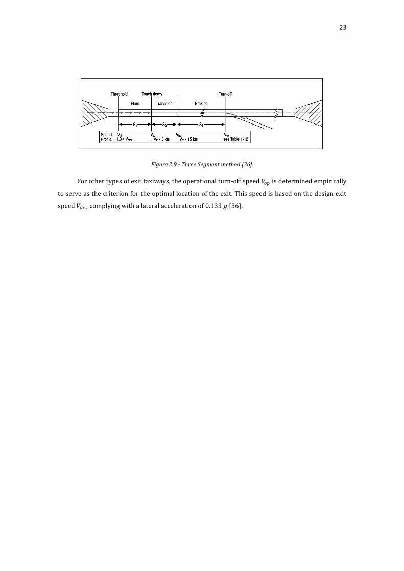
23

Figure 2.9 - Three Segment method [36].

For other types of exit taxiways, the operational turn-off speed 𝑉𝑜𝑝 is determined empirically

to serve as the criterion for the optimal location of the exit. This speed is based on the design exit

speed 𝑉𝑑𝑒𝑠 complying with a lateral acceleration of 0.133 𝑔 [36].

24

3 Performance Assessment Modelling

As mentioned before, two of the major performance measures of ATM systems are capacity

and delay. A large number of models have been developed over the years for these purposes. In fact,

this is the oldest area of model development in the ATM field, with the first significant models dating

back to the late 1950s. It is also the area where the most advanced modeling capabilities currently

exist [38] . Next, the different modelling approaches are analyzed.

Model Classification

According to Odoni et al, usually, airport models are classified with respect to three aspects:

coverage, methodology and level of detail [38]. According to the model coverage, airfield models can

be grouped according to their main focus: models focused on the runway system, the taxiway system,

the apron area, or integrated models (complete airfield). The majority of models cover runway

systems because this airfield element is the greatest capacity constraining factor, as it will be

discussed next. There are also a few models for taxiway systems. On the other hand, the apron area

is usually modelled as a part of integrated microscopic models and there are no generic models for

aprons suitable for quick assessment of apron area capacity.

With respect to methodology, models can be divided into analytical and simulation models.

Analytical models consist of a set of simplified mathematical relations that represent the real world.

Simulation models move individual objects through the system elements. Based on the parameters

and flow intersections of each entity, the time which objects spend in each segment of the system is

determined, and consequently system performance and the LOS. According to whether they are

analytical or simulation, models can be: dynamic(static), and stochastic(deterministic). Dynamic

models will capture the fluctuations over time in the performance metrics using as inputs time-

dependent parameters. Stochastic models will capture the impacts of uncertainty on the

performance metrics using as inputs parameters which are specified probabilistically, i.e. random or

pseudo-random variables.

In general, in simulation modelling, there are four major paradigms (Figure 3.1). In airfield

modelling, mainly two of those approaches are used: Discrete Event Simulation (DES) and Agent

Based Simulation (ABS). The first approach, is based on the concept of entities, resources and

flowcharts and/or networks describing entity flow and resource sharing [39]. Entities are passive

objects that represent tasks, vehicles, people and so on. They move through the blocks, where they

may, for example, wait in a queue, be processed or split. There are several commercial tools for this

modelling approach, which one targeting for particular businesses or purposes. Despite having

different interfaces, underneath they all have similar discrete event mechanisms that allow entities

to flow through the blocks, resulting in a global processing method.

25

With the second method, the modeler defines behavior at individual level and, unlike DES, the

global behavior results from many individual’s activities, each one with its own rules (also called

bottom-up modelling). Usually, for describing and analyzing a complex problem, the best

methodology is to use different modelling paradigms for different parts of the simulation model:

multi-paradigm commercial tools, such as AnyLogic [40]. But in airfield modelling, ABS approach

may be sufficient for some types of studies as it allows the construction of more complex models in

the absence of the knowledge about the global interdependencies. Moreover, the geographical and

functional distribution and the highly dynamic nature of ATC make it an ideal candidate with many

potential applications that can be modeled with Multi-Agent Systems (MAS), i.e. systems modelled

by a collection of agents [41].

Figure 3.1 - Simulation paradigms on abstraction level scale [42].

Simulation models may also be classified according to their level of detail as macroscopic or

microscopic. The first, omit a great deal of detail, since their objective is to obtain approximate

answers, with lower granularity. These models are used primarily for planning purposes, some

design issues and cost-benefit evaluation. Ideally they should be fast, in terms of both input

preparation and execution times, so they can be used to explore a large number of scenarios. Airfield

microscopic models use highly faithful representation of the various processes that take place at the

airport. Typically, such models represent aircraft on an individual basis and move them through the

ATM elements, which are represented by the model. They take into consideration each aircraft’s

performance characteristics. Such detailed features as the airport’s taxiway and gate selection,

pushback maneuvering, and so on, are generally included only in microscopic models.

26

In practice, according to Transport Research Board, depending on their applications,

assumptions, the data, time and cost requirements, the model availability and the skill/training

required for the operator, five levels of airfield modelling sophistication can be defined [7]:

1. Table Lookup;

2. Charts, Nomographs, and Spreadsheets;

3. Analytical Capacity Models;

4. Airfield Capacity Simulation Models and

5. Aircraft Delay Simulation Models.

The difference between the last two levels as to do mainly with the level of detail and

sophistication and the input data needed for their use. Then, as they overlap in most of their

characteristics, hereafter they are going to be grouped and simply named “Simulation Models”. The

first two levels are self-explanatory, i.e in these levels of sophistication, capacity analyses are

accomplished using table reference, charts, nomographs and spreasheets. For that reason, and since

analytical methods are used as basis for the simulation models, the last three levels are reviewed

next.

Analytical Models

The basis for analytical probabilistic models for runway capacity estimation, in conditions of

saturation, was set by Blumstein [19]. He set the method for calculating landing capacity for a single

runway as the mean time interval between two consecutive passes “over” the runway threshold. That

mean time interval depends on the length of the common final approach path and on separation

requirements at final approach set by the ATM. Mean inter-arrival time also depends on the fleet mix.

This is a common approach, even today, when estimating the landing capacity of a runway. All other

analytical models can be defined as extensions or modifications of Blumstein method.

According to Ashford et. al, the first improvement in Blumstein model was done by Harris [10].

He adapted the model for departures and mixed operations, and introduced stochastic to aircraft

arrival at the final approach fix [43]. After that, Hockaday et. al, upgraded Harris’ model. In their

model, they considered the effect of wake turbulence created by large jet aircraft separations, and

the derivation of optimal operating strategies for specific proportions of arrivals and departures in

the mix. They were also the first to analyze the case of multiple runways with many configurations

[14].

27

Several authors studied the effect on the capacity estimation of introducing new procedures,

or technological improvements. These are the cases of Horonjeff and Tos̆ic that analyzed the effects

of the MLS (Microwave Landing System) introduction on runway landing capacity [44]. This new

system differs from the ILS by using multiple and curved approach paths to the runway whereas the

ILS describes only a single straight path. Another case, more recent, is Janice that developed

analytical models for calculating the ultimate arrival, departure, and mixed operation capacity of

closely-spaced parallel runways using innovative approach procedures, such as the Staggered

Approach Procedure (SGAP), the Steeper Approach Procedure (SEAP) in combination with the

baseline Conventional Approach Procedure (CNAP) under IMC and IFR [45].

Based on Blumstein method, several models were created by translating into computer

language what was established before. That is the case of the FAA Capacity Model (FACM) and the

LMI Capacity and Delays Model. The FACM estimates capacity for 15 different common runway

configurations, ranging from one to four simultaneously active runways. These configurations are

observed as the combination of 4 fundamental configurations: single runway, closely-spaced parallel

(dependent), medium-spaced parallel (independent departures) and crossed runways. The first

version of FACM is developed during the 1970s by Peat, Marwick, Mitchell and Company and

McDonnell Douglas Automation, which was later modified by the FAA supported by the MITRE

Corporation (Enhanced FAA Airfield Capacity Model) [38].

According to Odoni et al, the LMI Capacity Model main objective is to obtain the "runway

capacity curve", i.e., the set of points that define the envelope of the maximum throughput capacities

that can be achieved at a single runway, under the entire range of possible arrival and departure

mixes. The model determines four points on the runway capacity curve. By interpolating between

pairs of points with straight-line segments, one can then obtain (approximately) the full runway

capacity curve. The four points are the following [38]:

Point 1: The "all arrivals" point, i.e., the capacity of the runway when it is used for arrivals

only.

Point 2: The "freely inserted departures" point which has the same arrival capacity as Point

1 and a capacity for departures equal to the number of departures that can be inserted into

the arrival stream "for free", i.e., by exploiting large inter-arrival gaps without increasing the

separations between successive arrivals (and, thus, without reducing the number of arrivals

from what can be achieved in the all-arrivals case).

Point 3: The "alternating arrivals and departures" point, i.e., the point at which an equal

number of departures and arrivals is performed. This is achieved through an arrival-

departure-arrival-departure sequencing, implemented by "stretching", when necessary, the

inter-arrival gaps, so that a departure can always be inserted between two successive

arrivals.

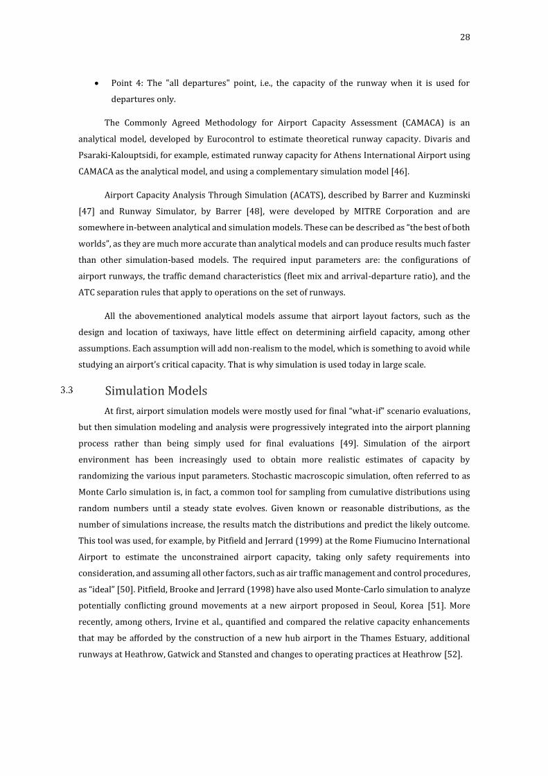
28

Point 4: The "all departures" point, i.e., the capacity of the runway when it is used for

departures only.

The Commonly Agreed Methodology for Airport Capacity Assessment (CAMACA) is an

analytical model, developed by Eurocontrol to estimate theoretical runway capacity. Divaris and

Psaraki-Kalouptsidi, for example, estimated runway capacity for Athens International Airport using

CAMACA as the analytical model, and using a complementary simulation model [46].

Airport Capacity Analysis Through Simulation (ACATS), described by Barrer and Kuzminski

[47] and Runway Simulator, by Barrer [48], were developed by MITRE Corporation and are

somewhere in-between analytical and simulation models. These can be described as “the best of both

worlds”, as they are much more accurate than analytical models and can produce results much faster

than other simulation-based models. The required input parameters are: the configurations of

airport runways, the traffic demand characteristics (fleet mix and arrival-departure ratio), and the

ATC separation rules that apply to operations on the set of runways.

All the abovementioned analytical models assume that airport layout factors, such as the

design and location of taxiways, have little effect on determining airfield capacity, among other

assumptions. Each assumption will add non-realism to the model, which is something to avoid while

studying an airport’s critical capacity. That is why simulation is used today in large scale.

Simulation Models

At first, airport simulation models were mostly used for final “what-if” scenario evaluations,

but then simulation modeling and analysis were progressively integrated into the airport planning

process rather than being simply used for final evaluations [49]. Simulation of the airport

environment has been increasingly used to obtain more realistic estimates of capacity by

randomizing the various input parameters. Stochastic macroscopic simulation, often referred to as

Monte Carlo simulation is, in fact, a common tool for sampling from cumulative distributions using

random numbers until a steady state evolves. Given known or reasonable distributions, as the

number of simulations increase, the results match the distributions and predict the likely outcome.

This tool was used, for example, by Pitfield and Jerrard (1999) at the Rome Fiumucino International

Airport to estimate the unconstrained airport capacity, taking only safety requirements into

consideration, and assuming all other factors, such as air traffic management and control procedures,

as “ideal” [50]. Pitfield, Brooke and Jerrard (1998) have also used Monte-Carlo simulation to analyze

potentially conflicting ground movements at a new airport proposed in Seoul, Korea [51]. More

recently, among others, Irvine et al., quantified and compared the relative capacity enhancements

that may be afforded by the construction of a new hub airport in the Thames Estuary, additional

runways at Heathrow, Gatwick and Stansted and changes to operating practices at Heathrow [52].

29

There are no regimentations about the standardized employment of capacity analysis and

simulation. However, most research has been implementing the same methodologies, with small

differences depending on several factors, such as the software used. As referred before, microscopic

simulation models generate traffic flows through the airspace and airport segments. Observations

from these flows allow appropriate measures of capacity and/or delay to be computed. Microscopic

models, can be either node-link or 3-Dimensional (3-D). Node-link models such as the Airport and

Airspace Simulation Model (SIMMOD) and the Airport Machine separate the airport and airspace into

a number of nodes and links over which aircraft move. Conflict occurs when more than one aircraft

tries to pass one node. 3-D models such as Total Aispace and Airport Modeller (TAAM) and Heuristic

Runway Movement Event Simulation (HERMES), allow flight over random 3-Dimensional routes

[38]. Most of the literature reviewed that used SIMMOD followed essentially the same steps to study

maximum capacities for baseline and alternative scenarios [53] [54] [55]:

1. Modeling of existing conditions and calibration with respect to hourly runway throughput

and delay.

2. Cloning using constant demand increments.

3. Making curve estimation: carry out curve fitting test, significance test and parameter

estimates.

4. Summarizing and calculating average delays of each cloning scenario. Then, usually, the next

step is to estimate at which rate of demand and under which scenario the service rate is

exceeded, flights are delayed and the average delays increase above predefined LOS.

In the case of the literature found for TAAM, the authors analyzed three capacity measures for

each scenario. This way, they compare the different scenarios in terms of: efficiency/design

functionality; sensitivity to technological/procedural improvements and overall utilization of

potential capacity. These are, essentially, saturation capacities of each layout constrained at varying

levels [56] [57]:

Fully constrained capacity (𝜆𝑠1): Capacity as influenced by all constraints incumbent at an

airport - ground as well as airspace constraints,

Semi-constrained capacity (𝜆𝑠2): Capacity under procedural and technological constraints -

only Airspace constraints,

Unconstrained capacity (𝜆𝑠3): Capacity in an unconstrained environment considering only

safety related constraints such as separation standards.

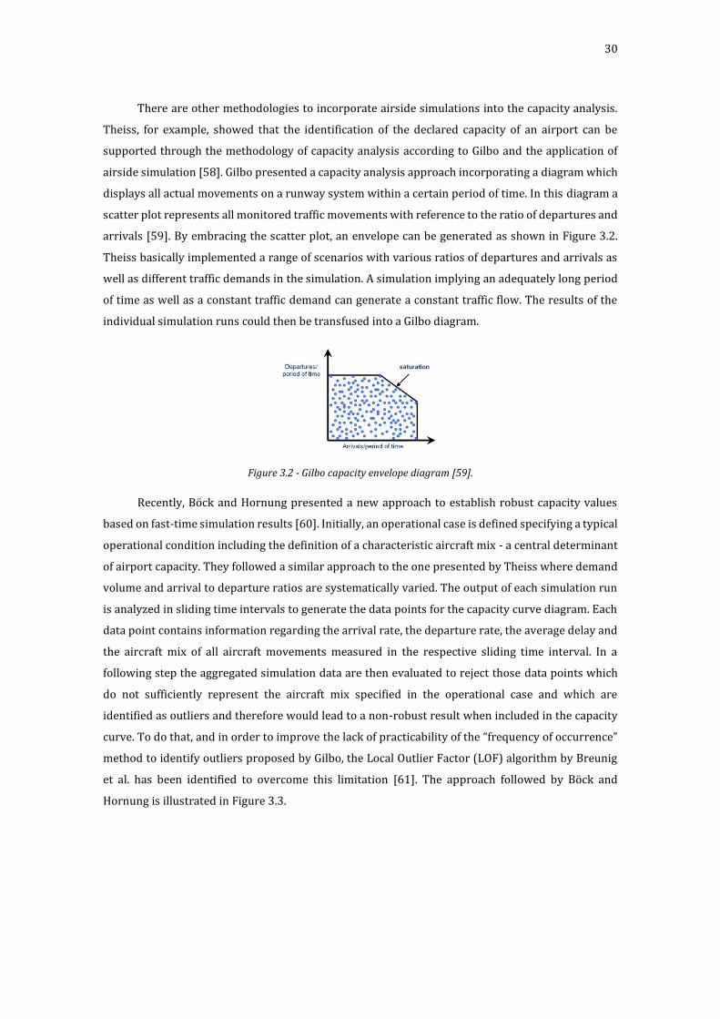
30

There are other methodologies to incorporate airside simulations into the capacity analysis.

Theiss, for example, showed that the identification of the declared capacity of an airport can be

supported through the methodology of capacity analysis according to Gilbo and the application of

airside simulation [58]. Gilbo presented a capacity analysis approach incorporating a diagram which

displays all actual movements on a runway system within a certain period of time. In this diagram a

scatter plot represents all monitored traffic movements with reference to the ratio of departures and

arrivals [59]. By embracing the scatter plot, an envelope can be generated as shown in Figure 3.2.

Theiss basically implemented a range of scenarios with various ratios of departures and arrivals as

well as different traffic demands in the simulation. A simulation implying an adequately long period

of time as well as a constant traffic demand can generate a constant traffic flow. The results of the

individual simulation runs could then be transfused into a Gilbo diagram.

Figure 3.2 - Gilbo capacity envelope diagram [59].

Recently, Böck and Hornung presented a new approach to establish robust capacity values

based on fast-time simulation results [60]. Initially, an operational case is defined specifying a typical

operational condition including the definition of a characteristic aircraft mix - a central determinant

of airport capacity. They followed a similar approach to the one presented by Theiss where demand

volume and arrival to departure ratios are systematically varied. The output of each simulation run

is analyzed in sliding time intervals to generate the data points for the capacity curve diagram. Each

data point contains information regarding the arrival rate, the departure rate, the average delay and

the aircraft mix of all aircraft movements measured in the respective sliding time interval. In a

following step the aggregated simulation data are then evaluated to reject those data points which

do not sufficiently represent the aircraft mix specified in the operational case and which are

identified as outliers and therefore would lead to a non-robust result when included in the capacity

curve. To do that, and in order to improve the lack of practicability of the “frequency of occurrence”

method to identify outliers proposed by Gilbo, the Local Outlier Factor (LOF) algorithm by Breunig

et al. has been identified to overcome this limitation [61]. The approach followed by Böck and

Hornung is illustrated in Figure 3.3.

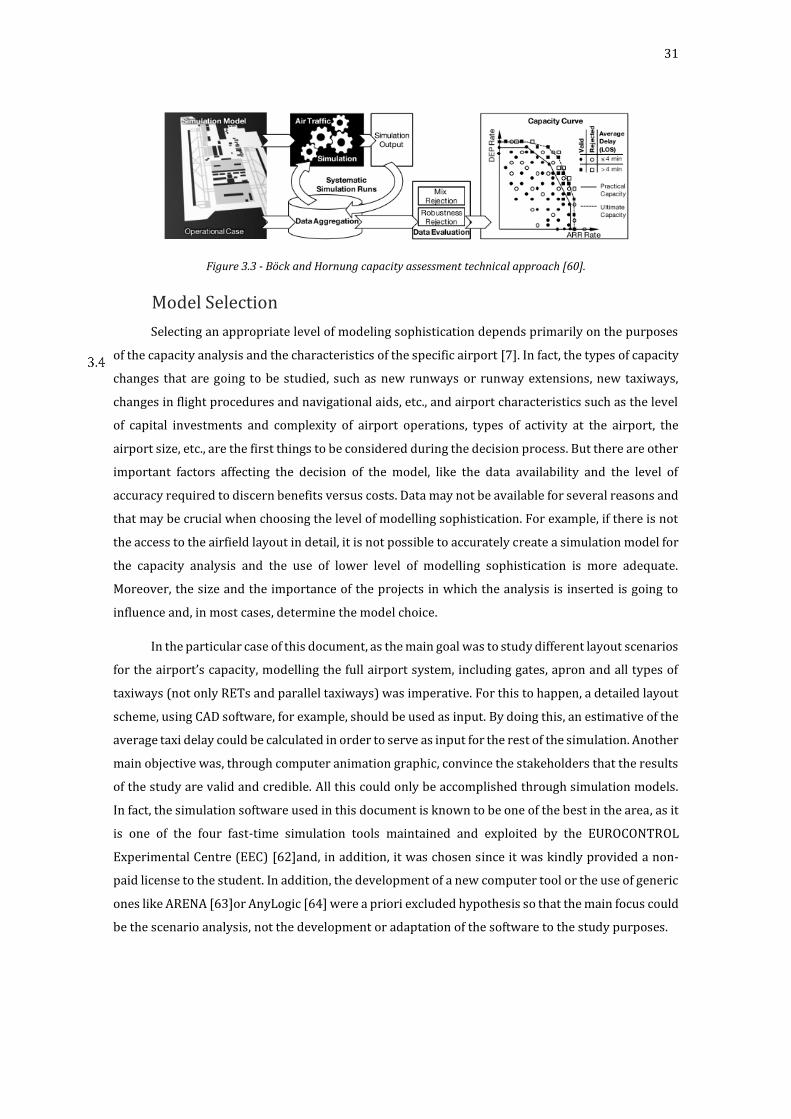
31

Figure 3.3 - Böck and Hornung capacity assessment technical approach [60].

Model Selection

Selecting an appropriate level of modeling sophistication depends primarily on the purposes

of the capacity analysis and the characteristics of the specific airport [7]. In fact, the types of capacity

changes that are going to be studied, such as new runways or runway extensions, new taxiways,

changes in flight procedures and navigational aids, etc., and airport characteristics such as the level

of capital investments and complexity of airport operations, types of activity at the airport, the

airport size, etc., are the first things to be considered during the decision process. But there are other

important factors affecting the decision of the model, like the data availability and the level of

accuracy required to discern benefits versus costs. Data may not be available for several reasons and

that may be crucial when choosing the level of modelling sophistication. For example, if there is not

the access to the airfield layout in detail, it is not possible to accurately create a simulation model for

the capacity analysis and the use of lower level of modelling sophistication is more adequate.

Moreover, the size and the importance of the projects in which the analysis is inserted is going to

influence and, in most cases, determine the model choice.

In the particular case of this document, as the main goal was to study different layout scenarios

for the airport’s capacity, modelling the full airport system, including gates, apron and all types of

taxiways (not only RETs and parallel taxiways) was imperative. For this to happen, a detailed layout

scheme, using CAD software, for example, should be used as input. By doing this, an estimative of the

average taxi delay could be calculated in order to serve as input for the rest of the simulation. Another

main objective was, through computer animation graphic, convince the stakeholders that the results

of the study are valid and credible. All this could only be accomplished through simulation models.

In fact, the simulation software used in this document is known to be one of the best in the area, as it

is one of the four fast-time simulation tools maintained and exploited by the EUROCONTROL

Experimental Centre (EEC) [62]and, in addition, it was chosen since it was kindly provided a non-

paid license to the student. In addition, the development of a new computer tool or the use of generic

ones like ARENA [63]or AnyLogic [64] were a priori excluded hypothesis so that the main focus could

be the scenario analysis, not the development or adaptation of the software to the study purposes.

32

The software used in this document for simulation analysis is called Comprehensive Airport

Simulation Tool (CAST) developed by Airport Research Center GmbH (ARC). CAST is a high-

performance 2D/3D fast time PC-based simulation system for modeling and evaluating airport-

systems, traffic and processes. CAST is based on multi-agent technology: every passenger, vehicle or

aircraft is an individual agent and able to react to the given situation according its individual goals,

intentions and characteristics.

Figure 3.4 - CAST Aircraft caption [65].

CAST is made of three modules: CAST Terminal, CAST Vehicle and CAST Aircraft. Each module

may be used as a stand-alone application or together with other CAST modules. The first one presents

detailed and realistic 3D models of airport terminals and other buildings to enable decision support,

planning, design and analysis. The second one, evaluates airside ground traffic, providing an accurate

model of microscopic driving behavior: vehicles accelerate, turn, change lanes and overtake

according to their kinematic and dynamic properties and give way at road junctions obeying the

respective traffic rules. CAST Aircraft is the module used in this document simulations. It simulates

the aircraft traffic at and around airports considering infrastructure, rules, restrictions, and

operational strategies [65].

33

4 Work Methodology

The methodology followed can be divided in two stages. In the first stage, based on the

available data, the baseline airport model is created and tested. In the second stage, alternatives are

tested and the results are compared to the reference scenario.

Technical Approach

In addition to the airport layout structure, based on charts presented in the Airport

Information Publication (AIP), ground movement and terminal airspace restrictions are entered in

the model. Then, to test the model, traffic is generated using typical/historical values for the inputs.

Besides the airport layout, the main inputs for the model are: the aircraft separation

requirements, the aircraft fleet mix and the runway exits usage distribution. The separation between

aircraft is based on ICAO’s critical values, i.e. those that lead to maximum runway capacity. In terms

of aircraft fleet mix, a compromise is obviously required between a very precise categorization of

aircraft types and the need to keep the number of movement types down to manageable levels for

modelling purposes. Two characteristics of aircraft which have an important effect on times are

weight and speed. Weight is the dominant factor and acts via the wake turbulence separation. For

the purpose of specifying the wake turbulence separations, aircraft are usually divided into three

main weight classes. Speed determines the runway occupancy times as well as the travel times over

certain specified separation distances on the approach and departure paths. An independent division

of aircraft according to both weight and speed could lead to a large number of types. For civilian

aircraft, a rough correlation between weight and speed can be made: the heavier aircraft tend to be

faster. This way, for the capacity analysis it is sufficient to distinguish heavy, medium and light

aircraft and to adopt typical mean speed and accelerations for each class [15]. In this document, as

explained later, the aircraft categorization will only act via wake turbulence separation and through

the runway exit distribution, since the mean speeds and accelerations were equally defined for the

three classes.

The arrival aircraft are then distributed by the runway exits according to their type. Both

aircraft fleet mix and the exits usage distribution are entered as fixed probabilities which will result

in different outputs since CAST uses a (pseudo)random seed to produce different distributions of

those shares over the simulation time.

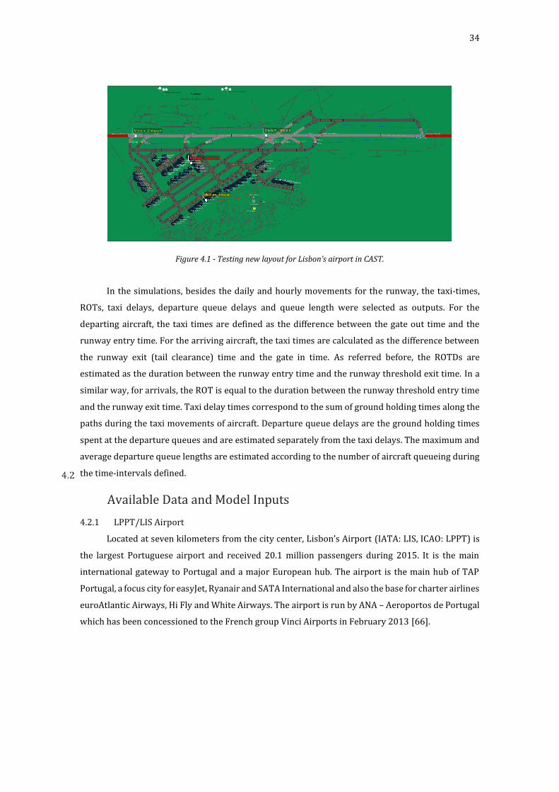
34

Figure 4.1 - Testing new layout for Lisbon’s airport in CAST.

In the simulations, besides the daily and hourly movements for the runway, the taxi-times,

ROTs, taxi delays, departure queue delays and queue length were selected as outputs. For the

departing aircraft, the taxi times are defined as the difference between the gate out time and the

runway entry time. For the arriving aircraft, the taxi times are calculated as the difference between

the runway exit (tail clearance) time and the gate in time. As referred before, the ROTDs are

estimated as the duration between the runway entry time and the runway threshold exit time. In a

similar way, for arrivals, the ROT is equal to the duration between the runway threshold entry time

and the runway exit time. Taxi delay times correspond to the sum of ground holding times along the

paths during the taxi movements of aircraft. Departure queue delays are the ground holding times

spent at the departure queues and are estimated separately from the taxi delays. The maximum and

average departure queue lengths are estimated according to the number of aircraft queueing during

the time-intervals defined.

Available Data and Model Inputs

4.2.1 LPPT/LIS Airport

Located at seven kilometers from the city center, Lisbon’s Airport (IATA: LIS, ICAO: LPPT) is

the largest Portuguese airport and received 20.1 million passengers during 2015. It is the main

international gateway to Portugal and a major European hub. The airport is the main hub of TAP

Portugal, a focus city for easyJet, Ryanair and SATA International and also the base for charter airlines

euroAtlantic Airways, Hi Fly and White Airways. The airport is run by ANA – Aeroportos de Portugal

which has been concessioned to the French group Vinci Airports in February 2013 [66].

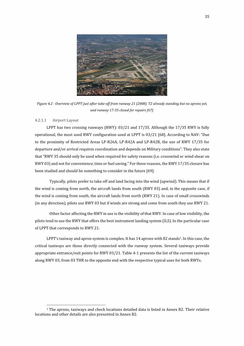
35

Figure 4.2 - Overview of LPPT just after take-off from runway 21 (2008). T2 already standing but no aprons yet,

and runway 17-35 closed for repairs [67].

4.2.1.1 Airport Layout

LPPT has two crossing runways (RWY): 03/21 and 17/35. Although the 17/35 RWY is fully

operational, the most used RWY configuration used at LPPT is 03/21 [68]. According to NAV: “Due

to the proximity of Restricted Areas LP-R26A, LP-R42A and LP-R42B, the use of RWY 17/35 for

departure and/or arrival requires coordination and depends on Military conditions”. They also state

that “RWY 35 should only be used when required for safety reasons (i.e. crosswind or wind shear on

RWY 03) and not for convenience, time or fuel saving.” For these reasons, the RWY 17/35 closure has

been studied and should be something to consider in the future [69].

Typically, pilots prefer to take off and land facing into the wind (upwind). This means that if

the wind is coming from north, the aircraft lands from south (RWY 03) and, in the opposite case, if

the wind is coming from south, the aircraft lands from north (RWY 21). In case of small crosswinds

(in any direction), pilots use RWY 03 but if winds are strong and come from south they use RWY 21.

Other factor affecting the RWY in use is the visibility of that RWY. In case of low visibility, the

pilots tend to use the RWY that offers the best instrument landing system (ILS). In the particular case

of LPPT that corresponds to RWY 21.

LPPT’s taxiway and apron system is complex. It has 14 aprons with 82 stands1. In this case, the

critical taxiways are those directly connected with the runway system. Several taxiways provide

appropriate entrance/exit points for RWY 03/21. Table 4-1 presents the list of the current taxiways

along RWY 03, from 03 THR to the opposite end with the respective typical uses for both RWYs.

1 The aprons, taxiways and check locations detailed data is listed in Annex B2. Their relative

locations and other details are also presented in Annex B2.

36

Taxiway Purpose

RWY 03 RWY 21

M5 Entrance Exit

N2 Entrance Exit

P Entrance Exit

RET HS - Exit

RWY 17 Exit -

S1 Exit -

RET HN Exit -

U5 Exit Entrance

S4 Exit Entrance

Table 4-1 - Current taxiways serving RWY 03.

4.2.1.2 Terminal Airspace

Lisbon’s terminal airspace is divided into four sectors: TMA Upper Sector, TMA Lower Sector,

APP Sector 1 and APP Sector 2. It is usual to refer to Lisbon’s terminal area simply as TMA and

Approach Control Position (APP). APP covers an 30NM circular arc area centred in LPPT’s reference

point and limited west by TMA (Figure 4.3). APP is responsible for separation of aircraft on TMA and

Vectoring Area until transfer of control point. Tower (TWR) is responsible after established on ILS

approach. ILS approach chart for RWY 03 is in Annex B.4.

Figure 4.3 - LPPT terminal airspace: TMA and APP sector [70].

There are SIDs and STARs published for, respectively, traffic departing from and arriving at

Lisbon. RWYs 03 and 35 share the standard procedures. These two RWYs have eleven SIDs and

twelve STARs.

For the inbound traffic, these are the maximum speeds allowed [3]:

280KT IAS between FL245 and FL100;

250KT IAS at and below FL100;

220KT IAS at and below FL070

200KT IAS at and below 4000ft;

Between 160 and 180KT IAS when established on final approach segment;

160KT IAS until 4NM from RWY threshold.

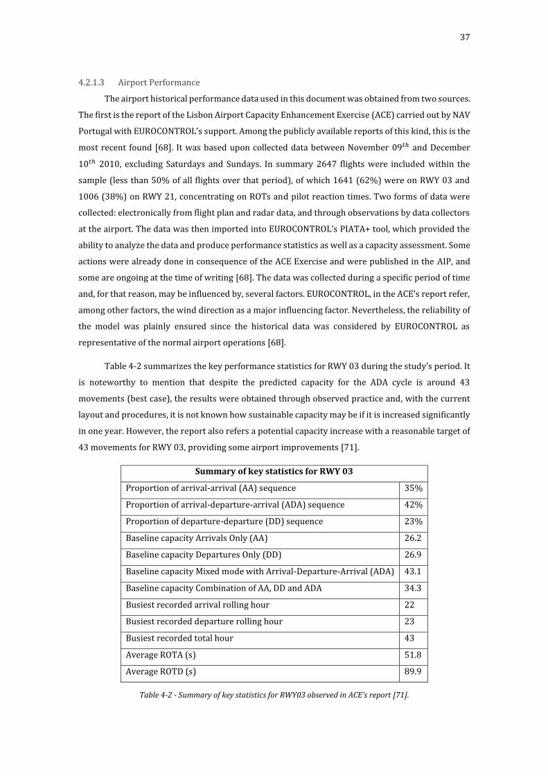
37

4.2.1.3 Airport Performance

The airport historical performance data used in this document was obtained from two sources.

The first is the report of the Lisbon Airport Capacity Enhancement Exercise (ACE) carried out by NAV

Portugal with EUROCONTROL’s support. Among the publicly available reports of this kind, this is the

most recent found [68]. It was based upon collected data between November 09𝑡ℎ and December

10𝑡ℎ 2010, excluding Saturdays and Sundays. In summary 2647 flights were included within the

sample (less than 50% of all flights over that period), of which 1641 (62%) were on RWY 03 and

1006 (38%) on RWY 21, concentrating on ROTs and pilot reaction times. Two forms of data were

collected: electronically from flight plan and radar data, and through observations by data collectors

at the airport. The data was then imported into EUROCONTROL’s PIATA+ tool, which provided the

ability to analyze the data and produce performance statistics as well as a capacity assessment. Some

actions were already done in consequence of the ACE Exercise and were published in the AIP, and

some are ongoing at the time of writing [68]. The data was collected during a specific period of time

and, for that reason, may be influenced by, several factors. EUROCONTROL, in the ACE’s report refer,

among other factors, the wind direction as a major influencing factor. Nevertheless, the reliability of

the model was plainly ensured since the historical data was considered by EUROCONTROL as

representative of the normal airport operations [68].

Table 4-2 summarizes the key performance statistics for RWY 03 during the study’s period. It

is noteworthy to mention that despite the predicted capacity for the ADA cycle is around 43

movements (best case), the results were obtained through observed practice and, with the current

layout and procedures, it is not known how sustainable capacity may be if it is increased significantly

in one year. However, the report also refers a potential capacity increase with a reasonable target of

43 movements for RWY 03, providing some airport improvements [71].

Summary of key statistics for RWY 03

Proportion of arrival-arrival (AA) sequence 35%

Proportion of arrival-departure-arrival (ADA) sequence 42%

Proportion of departure-departure (DD) sequence 23%

Baseline capacity Arrivals Only (AA) 26.2

Baseline capacity Departures Only (DD) 26.9

Baseline capacity Mixed mode with Arrival-Departure-Arrival (ADA) 43.1

Baseline capacity Combination of AA, DD and ADA 34.3

Busiest recorded arrival rolling hour 22

Busiest recorded departure rolling hour 23

Busiest recorded total hour 43

Average ROTA (s) 51.8

Average ROTD (s) 89.9

Table 4-2 - Summary of key statistics for RWY03 observed in ACE’s report [71].

38

Typically, the daily variation in traffic for LPPT is very high. Usually there are two or three

hourly movements peaks (Figure 4.4). These peaks are usually between 0800-0859 UTC, 1400-1500

UTC and 2000-2100 UTC [3]. The first and last hourly peak correspond to the daily maximum

movements: 40 movements [3]. Between 1400 and 1500 UTC the peak is usually smaller and the

runway maximum throughput is 39 movements [3]. During the rest of the day, the hourly maximum

capacity is 38 movements [3].Typical daily traffic also indicates that, on an hourly basis, there are no

significant arrival or departure peaks, i.e. the proportion of arrivals and departures in each hour is

approximately the same.

Figure 4.4 - Average total movements during ACE’s report observation period [71].

The following Table 4-3 shows the average ROTA observed for RWY 03 for three aircraft types

(Heavy, Medium Jets and Medium Prop) and by exit for Medium Jets. It is shown the advantage of

using HN instead of S1 with a difference in ROTA of 7 seconds. ACE exercise also states that the aim

should be to target the 10.3% of medium jet aircraft that use S1. In fact, the 7 seconds difference

between HN and the worst case (S1) can make a great difference in terms of the RWY capacity.

RWY 03 ROTA (seconds)

Aircraft Group Exit Average

Heavy MedJet MedProp HN RWY17 S1 54.1

57.5 51.1 53.6 52 51 59

Table 4-3 - RWY 03 ROTA by aircraft group, exit and average [71].

In what concerns departures for RWY 03 observed in ACE’s report, Table 4-4 shows the key

components of departure runway occupancy time and the total ROTD.

Key Departure Intervals LUPT TOCD FRTT TOFT Total (ROTD)

Duration (seconds) 32.5 4.1 14.3 31.4 89.9

Table 4-4 - Key departure intervals and respective durations [71].

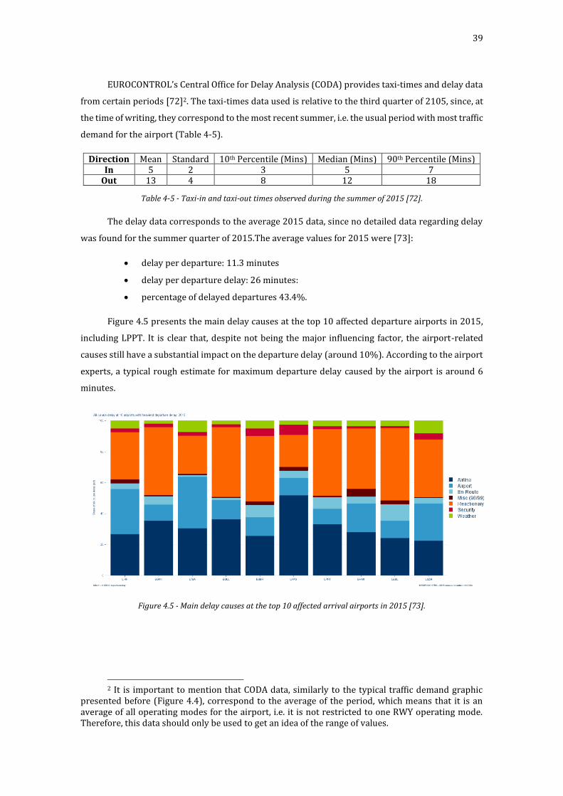
39

EUROCONTROL’s Central Office for Delay Analysis (CODA) provides taxi-times and delay data

from certain periods [72]2. The taxi-times data used is relative to the third quarter of 2105, since, at

the time of writing, they correspond to the most recent summer, i.e. the usual period with most traffic

demand for the airport (Table 4-5).

Direction Mean Standard 10th Percentile (Mins) Median (Mins) 90th Percentile (Mins) In 5 2 3 5 7

Out 13 4 8 12 18

Table 4-5 - Taxi-in and taxi-out times observed during the summer of 2015 [72].

The delay data corresponds to the average 2015 data, since no detailed data regarding delay

was found for the summer quarter of 2015.The average values for 2015 were [73]:

delay per departure: 11.3 minutes

delay per departure delay: 26 minutes:

percentage of delayed departures 43.4%.

Figure 4.5 presents the main delay causes at the top 10 affected departure airports in 2015,

including LPPT. It is clear that, despite not being the major influencing factor, the airport-related

causes still have a substantial impact on the departure delay (around 10%). According to the airport

experts, a typical rough estimate for maximum departure delay caused by the airport is around 6

minutes.

Figure 4.5 - Main delay causes at the top 10 affected arrival airports in 2015 [73].

2 It is important to mention that CODA data, similarly to the typical traffic demand graphic

presented before (Figure 4.4), correspond to the average of the period, which means that it is an average of all operating modes for the airport, i.e. it is not restricted to one RWY operating mode. Therefore, this data should only be used to get an idea of the range of values.

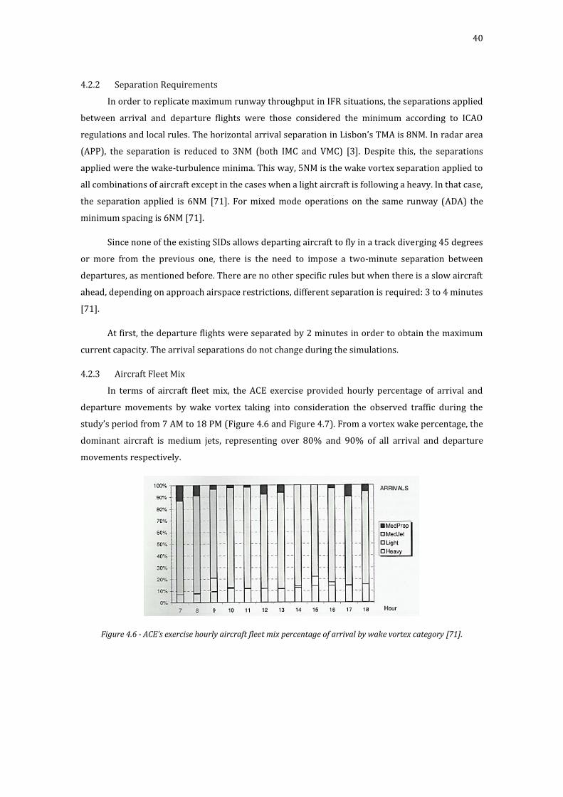
40

4.2.2 Separation Requirements

In order to replicate maximum runway throughput in IFR situations, the separations applied

between arrival and departure flights were those considered the minimum according to ICAO

regulations and local rules. The horizontal arrival separation in Lisbon’s TMA is 8NM. In radar area

(APP), the separation is reduced to 3NM (both IMC and VMC) [3]. Despite this, the separations

applied were the wake-turbulence minima. This way, 5NM is the wake vortex separation applied to

all combinations of aircraft except in the cases when a light aircraft is following a heavy. In that case,

the separation applied is 6NM [71]. For mixed mode operations on the same runway (ADA) the

minimum spacing is 6NM [71].

Since none of the existing SIDs allows departing aircraft to fly in a track diverging 45 degrees

or more from the previous one, there is the need to impose a two-minute separation between

departures, as mentioned before. There are no other specific rules but when there is a slow aircraft

ahead, depending on approach airspace restrictions, different separation is required: 3 to 4 minutes

[71].

At first, the departure flights were separated by 2 minutes in order to obtain the maximum

current capacity. The arrival separations do not change during the simulations.

4.2.3 Aircraft Fleet Mix

In terms of aircraft fleet mix, the ACE exercise provided hourly percentage of arrival and

departure movements by wake vortex taking into consideration the observed traffic during the

study’s period from 7 AM to 18 PM (Figure 4.6 and Figure 4.7). From a vortex wake percentage, the

dominant aircraft is medium jets, representing over 80% and 90% of all arrival and departure

movements respectively.

Figure 4.6 - ACE’s exercise hourly aircraft fleet mix percentage of arrival by wake vortex category [71].

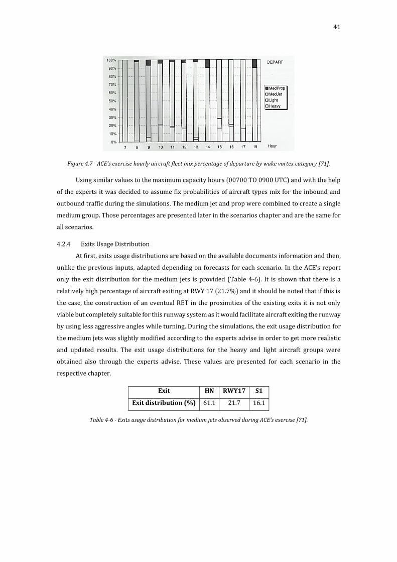
41

Figure 4.7 - ACE’s exercise hourly aircraft fleet mix percentage of departure by wake vortex category [71].

Using similar values to the maximum capacity hours (00700 TO 0900 UTC) and with the help

of the experts it was decided to assume fix probabilities of aircraft types mix for the inbound and

outbound traffic during the simulations. The medium jet and prop were combined to create a single

medium group. Those percentages are presented later in the scenarios chapter and are the same for

all scenarios.

4.2.4 Exits Usage Distribution

At first, exits usage distributions are based on the available documents information and then,

unlike the previous inputs, adapted depending on forecasts for each scenario. In the ACE’s report

only the exit distribution for the medium jets is provided (Table 4-6). It is shown that there is a

relatively high percentage of aircraft exiting at RWY 17 (21.7%) and it should be noted that if this is

the case, the construction of an eventual RET in the proximities of the existing exits it is not only

viable but completely suitable for this runway system as it would facilitate aircraft exiting the runway

by using less aggressive angles while turning. During the simulations, the exit usage distribution for

the medium jets was slightly modified according to the experts advise in order to get more realistic

and updated results. The exit usage distributions for the heavy and light aircraft groups were

obtained also through the experts advise. These values are presented for each scenario in the

respective chapter.

Exit HN RWY17 S1

Exit distribution (%) 61.1 21.7 16.1

Table 4-6 - Exits usage distribution for medium jets observed during ACE’s exercise [71].

42

Fast-time Simulations - CAST

4.3.1 Model Structure

As mentioned before, one advantage of the chosen simulation software is the ability to import

the layout from a Drawing Exchange Format (DXF) file to create the airport’s model structure. This

way it is much easier to create the model than creating the structure inside the simulation software.

The DXF file was based on a scale drawing chart of the airport in PDF format, present in the Annex A.

This chart is part of the AIP provided by the local Air Traffic Control company – NAV. Similar charts

were used to obtain other specific layout configuration characteristics, such as the stand locations

(Annex B.2). In cases where the charts didn’t provide enough information for a clear model creation,

Google Earth was used to get the objects disposition and sometimes, in very few cases, some

distances were obtained using its internal measurement tool by scaling according to foreknown 2D

distances.

Figure 4.8 illustrates how an airport layout should look like before importing the DXF into

CAST. Each infrastructure type is represented by a separate layer (layers may be of different colors).

Each element is represented by consecutive polylines with the respective straight or arc segments

(no splines) and junctions are automatically created where more than two lines meet.

Figure 4.8 - Current LPPT’s CAD model (DXF).

The infrastructure of a CAST Aircraft model consists of the following object elements: Airport,

Aircraft Stands, Taxiway Sections, Runway Sections and Airspace Sections (Figure 4.9).

Figure 4.9 - CAST Aircraft main infrastructure elements [65].

While the imported DXF layout may be a good baseline for the simulation modelling, before

validating the simulation setup, it requires some clean-ups, modifications and improvements, such

as: removing unnecessary sections and adjusting connecting elements of a junction in order to extend

these to an adequate size.

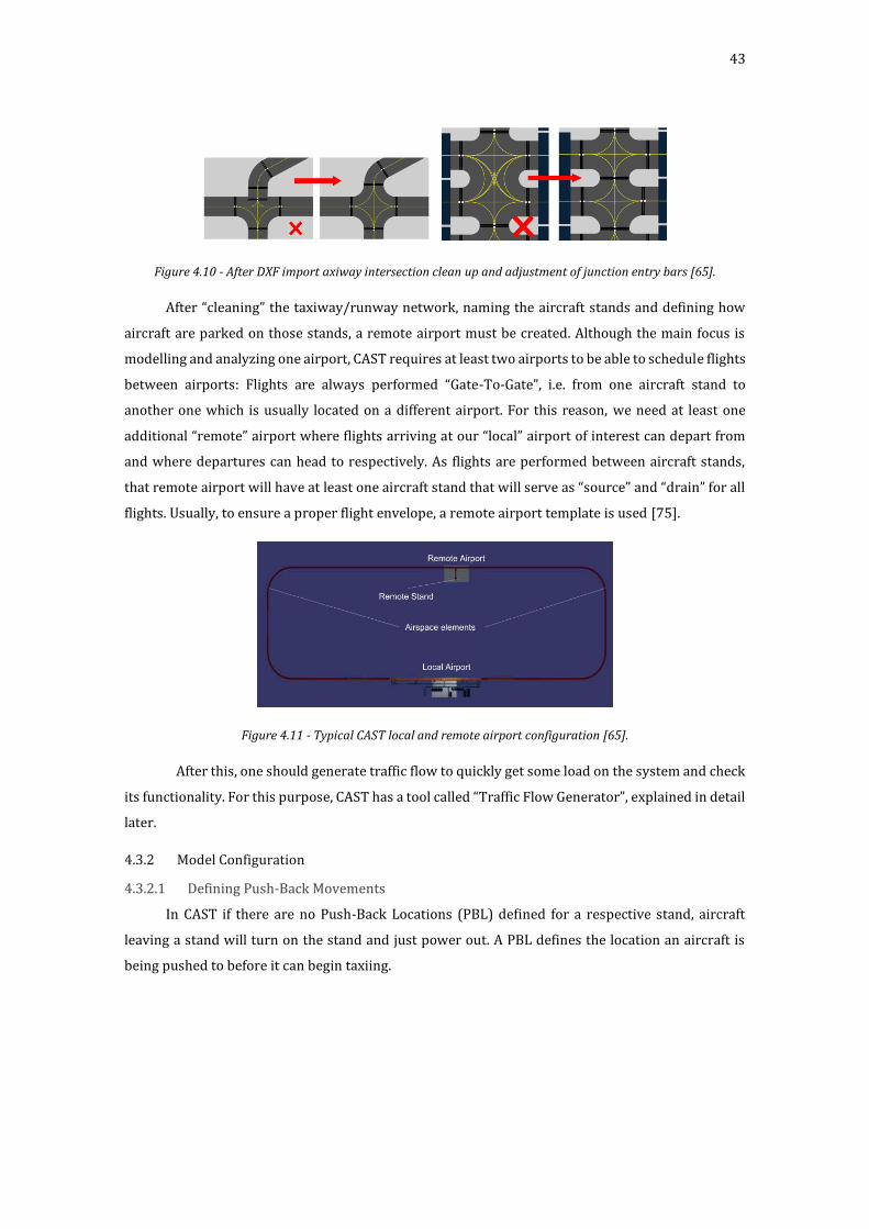
43

Figure 4.10 - After DXF import axiway intersection clean up and adjustment of junction entry bars [65].

After “cleaning” the taxiway/runway network, naming the aircraft stands and defining how

aircraft are parked on those stands, a remote airport must be created. Although the main focus is

modelling and analyzing one airport, CAST requires at least two airports to be able to schedule flights

between airports: Flights are always performed “Gate-To-Gate”, i.e. from one aircraft stand to

another one which is usually located on a different airport. For this reason, we need at least one

additional “remote” airport where flights arriving at our “local” airport of interest can depart from

and where departures can head to respectively. As flights are performed between aircraft stands,

that remote airport will have at least one aircraft stand that will serve as “source” and “drain” for all

flights. Usually, to ensure a proper flight envelope, a remote airport template is used [75].

Figure 4.11 - Typical CAST local and remote airport configuration [65].

After this, one should generate traffic flow to quickly get some load on the system and check

its functionality. For this purpose, CAST has a tool called “Traffic Flow Generator”, explained in detail

later.

4.3.2 Model Configuration

4.3.2.1 Defining Push-Back Movements

In CAST if there are no Push-Back Locations (PBL) defined for a respective stand, aircraft

leaving a stand will turn on the stand and just power out. A PBL defines the location an aircraft is

being pushed to before it can begin taxiing.

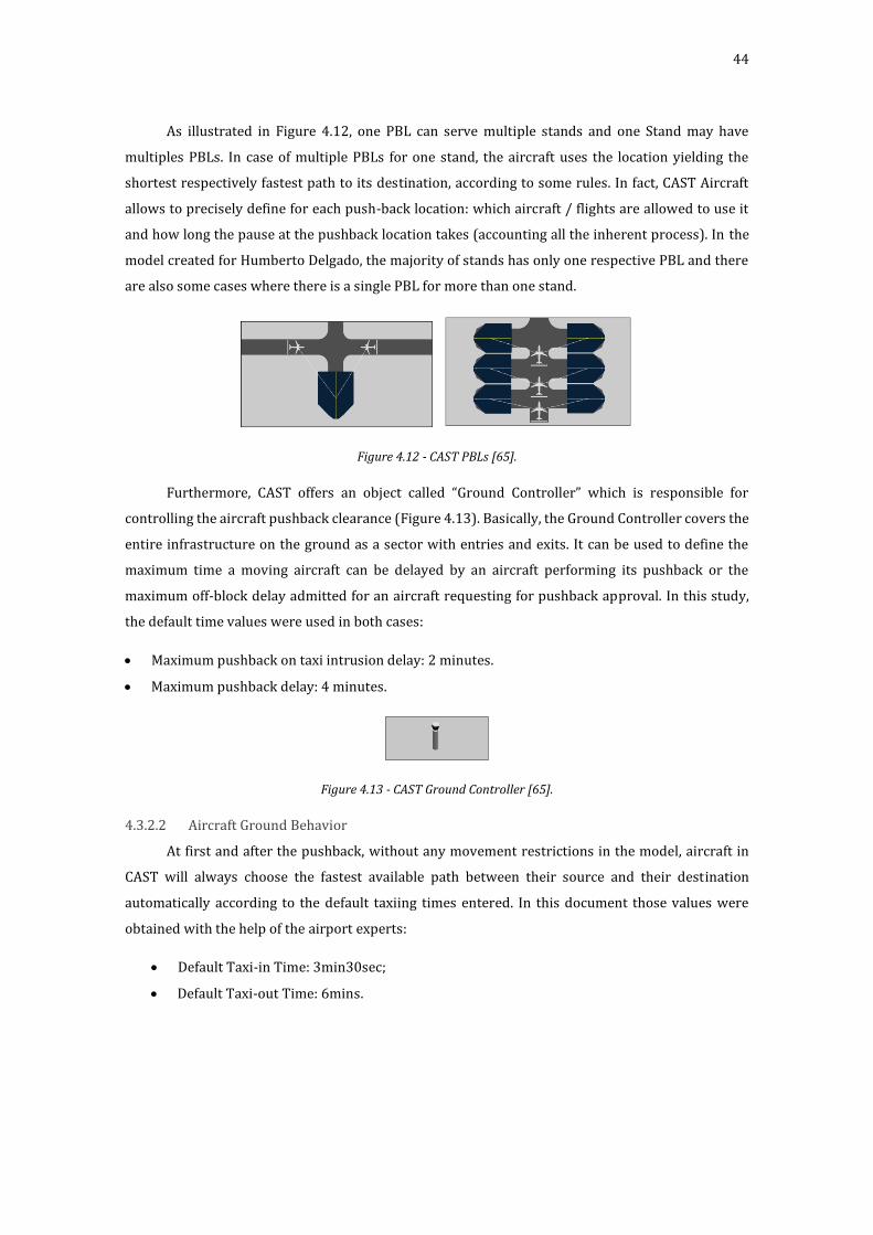
44

As illustrated in Figure 4.12, one PBL can serve multiple stands and one Stand may have

multiples PBLs. In case of multiple PBLs for one stand, the aircraft uses the location yielding the

shortest respectively fastest path to its destination, according to some rules. In fact, CAST Aircraft

allows to precisely define for each push-back location: which aircraft / flights are allowed to use it

and how long the pause at the pushback location takes (accounting all the inherent process). In the

model created for Humberto Delgado, the majority of stands has only one respective PBL and there

are also some cases where there is a single PBL for more than one stand.

Figure 4.12 - CAST PBLs [65].

Furthermore, CAST offers an object called “Ground Controller” which is responsible for

controlling the aircraft pushback clearance (Figure 4.13). Basically, the Ground Controller covers the

entire infrastructure on the ground as a sector with entries and exits. It can be used to define the

maximum time a moving aircraft can be delayed by an aircraft performing its pushback or the

maximum off-block delay admitted for an aircraft requesting for pushback approval. In this study,

the default time values were used in both cases:

Maximum pushback on taxi intrusion delay: 2 minutes.

Maximum pushback delay: 4 minutes.

Figure 4.13 - CAST Ground Controller [65].

4.3.2.2 Aircraft Ground Behavior

At first and after the pushback, without any movement restrictions in the model, aircraft in

CAST will always choose the fastest available path between their source and their destination

automatically according to the default taxiing times entered. In this document those values were

obtained with the help of the airport experts:

Default Taxi-in Time: 3min30sec;

Default Taxi-out Time: 6mins.

45

When calculating which is the fastest path to their destination aircraft will take into account:

Passage Restrictions;

The speed limitation of all guidelines used to reach the destination;

User-defined guideline costs;

The aircraft's speed;

The number of bends the aircraft has to take (as the speed is lower).

Therefore, in order to control the aircraft's routing through the model, it is possible to define

various restrictions:

Defining speed limitations on selected sections;

Set up user-defined costs on specific guidelines;

Defining restrictions depending on certain aircraft, flight or global properties;

Closing a path completely.

By default, in CAST Aircraft, each guideline can be used by each aircraft. But one can define

passages restrictions, defining which type of aircraft is allowed to use one particular guideline. For

example, one may allow the usage of some guideline only if the aircraft requesting permission are

Arrival aircraft. If there are multiple restrictions one can combine them: using “OR” (disjunction) or

“AND” (conjunction). In this study, besides some closing some paths completely, only two types of

passage restrictions were applied to guidelines, according to:

Flight Direction: first, in runway entrance taxiways, it was necessary to restrict the passage

to arrival aircraft. For runway exit taxiways, the opposite was applied: departure aircraft

cannot use the taxiway guideline.

Airport Operating Mode: restrict the routing of the aircraft according to the operating mode

of the airport, i.e. it was assumed that, during the simulation time, the airport is operating

with a single runway and that the aircraft should follow the routing concepts defined in the

Aerodrome Ground Movements Charts (Annex B.3). To do that, a property was created on

the airport, with the following parameters:

o Name: “Operation Mode”;

o Value Kind: “String”;

o Enumerated Values: 03, 21 (available runways).

In LPPT’s model, the ground dynamics were defined independently of the aircraft type. The

maximum linear and radial accelerations and speeds are presented in Table 4-7. The same applies to

the vehicle interaction: all vehicles must respect the same distance/time separations independently

of the leading/trailing aircraft (Table 4-9).

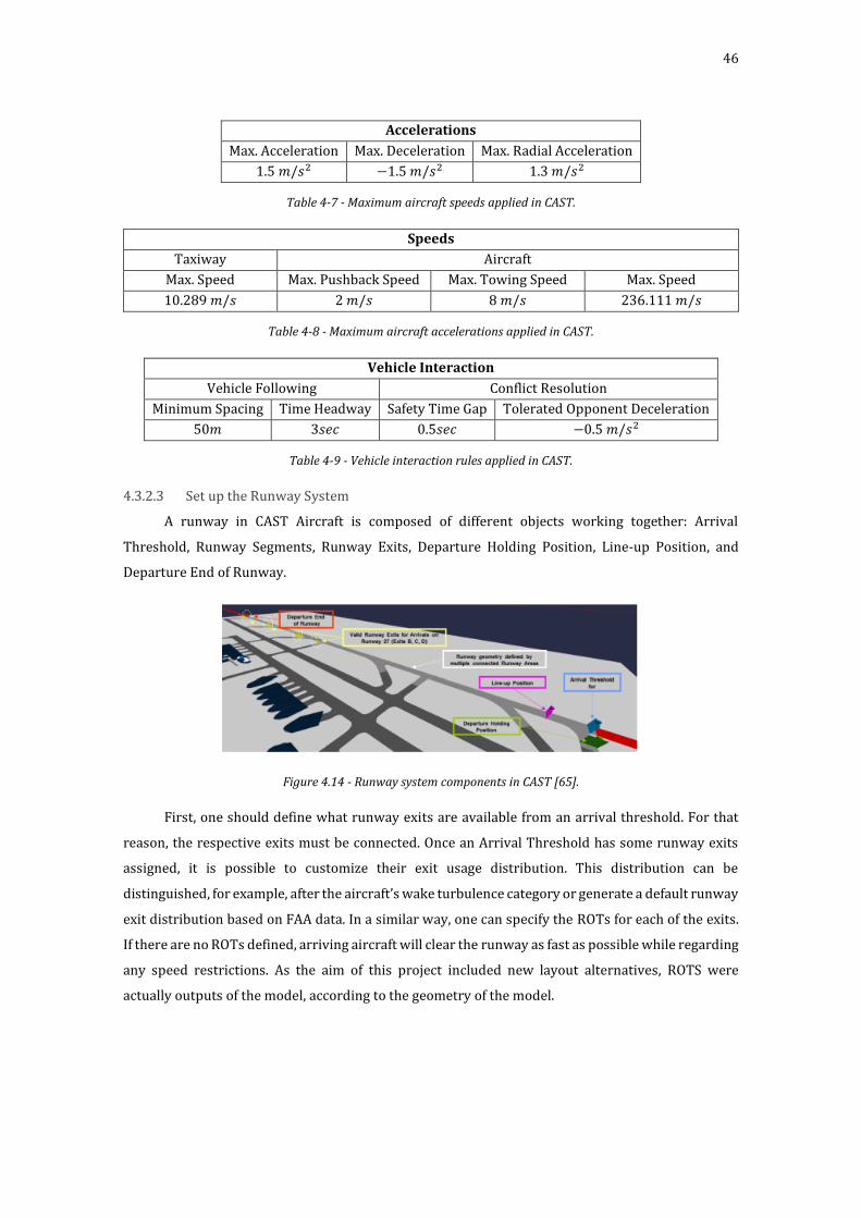
46

Accelerations

Max. Acceleration Max. Deceleration Max. Radial Acceleration

1.5 𝑚/𝑠2 −1.5 𝑚/𝑠2 1.3 𝑚/𝑠2

Table 4-7 - Maximum aircraft speeds applied in CAST.

Speeds

Taxiway Aircraft

Max. Speed Max. Pushback Speed Max. Towing Speed Max. Speed

10.289 𝑚/𝑠 2 𝑚/𝑠 8 𝑚/𝑠 236.111 𝑚/𝑠

Table 4-8 - Maximum aircraft accelerations applied in CAST.

Vehicle Interaction

Vehicle Following Conflict Resolution

Minimum Spacing Time Headway Safety Time Gap Tolerated Opponent Deceleration

50𝑚 3𝑠𝑒𝑐 0.5𝑠𝑒𝑐 −0.5 𝑚/𝑠2

Table 4-9 - Vehicle interaction rules applied in CAST.

4.3.2.3 Set up the Runway System

A runway in CAST Aircraft is composed of different objects working together: Arrival

Threshold, Runway Segments, Runway Exits, Departure Holding Position, Line-up Position, and

Departure End of Runway.

Figure 4.14 - Runway system components in CAST [65].

First, one should define what runway exits are available from an arrival threshold. For that

reason, the respective exits must be connected. Once an Arrival Threshold has some runway exits

assigned, it is possible to customize their exit usage distribution. This distribution can be

distinguished, for example, after the aircraft’s wake turbulence category or generate a default runway

exit distribution based on FAA data. In a similar way, one can specify the ROTs for each of the exits.

If there are no ROTs defined, arriving aircraft will clear the runway as fast as possible while regarding

any speed restrictions. As the aim of this project included new layout alternatives, ROTS were

actually outputs of the model, according to the geometry of the model.

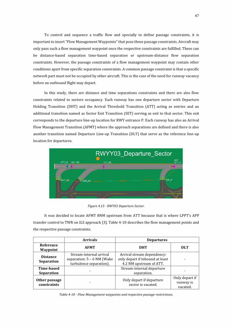
47

To control and sequence a traffic flow and specially to define passage constraints, it is

important to insert “Flow Management Waypoints” that pose those passage constraints. Aircraft may

only pass such a flow management waypoint once the respective constraints are fulfilled. These can

be distance-based separation time-based separation or upstream-distance flow separation

constraints. However, the passage constraints of a flow management waypoint may contain other

conditions apart from specific separation constraints. A common passage constraint is that a specific

network part must not be occupied by other aircraft. This is the case of the need for runway vacancy

before an outbound flight may depart.

In this study, there are distance and time separations constraints and there are also flow

constraints related to sectors occupancy. Each runway has one departure sector with Departure

Holding Transition (DHT) and the Arrival Threshold Transition (ATT) acting as entries and an

additional transition named as Sector Exit Transition (SET) serving as exit to that sector. This exit

corresponds to the departure line-up location for RWY entrance P. Each runway has also an Arrival

Flow Management Transition (AFMT) where the approach separations are defined and there is also

another transition named Departure Line-up Transition (DLT) that serve as the reference line-up

location for departures.

Figure 4.15 - RWY03 Departure Sector.

It was decided to locate AFMT 8NM upstream from ATT because that is where LPPT’s APP

transfer control to TWR on ILS approach [3]. Table 4-10 describes the flow management points and

the respective passage constraints.

Arrivals Departures

Reference Waypoint

AFMT DHT DLT

Distance Separation

Stream-internal arrival separation: 5 – 6 NM (Wake

turbulence separation).

Arrival stream dependency: only depart if inbound at least

4.2 NM upstream of ATT. -

Time-based Separation

- Stream-internal departure

separation. -

Other passage constraints

- Only depart if departure

sector is vacated.

Only depart if runway is vacated.

Table 4-10 - Flow Management waypoints and respective passage restrictions.

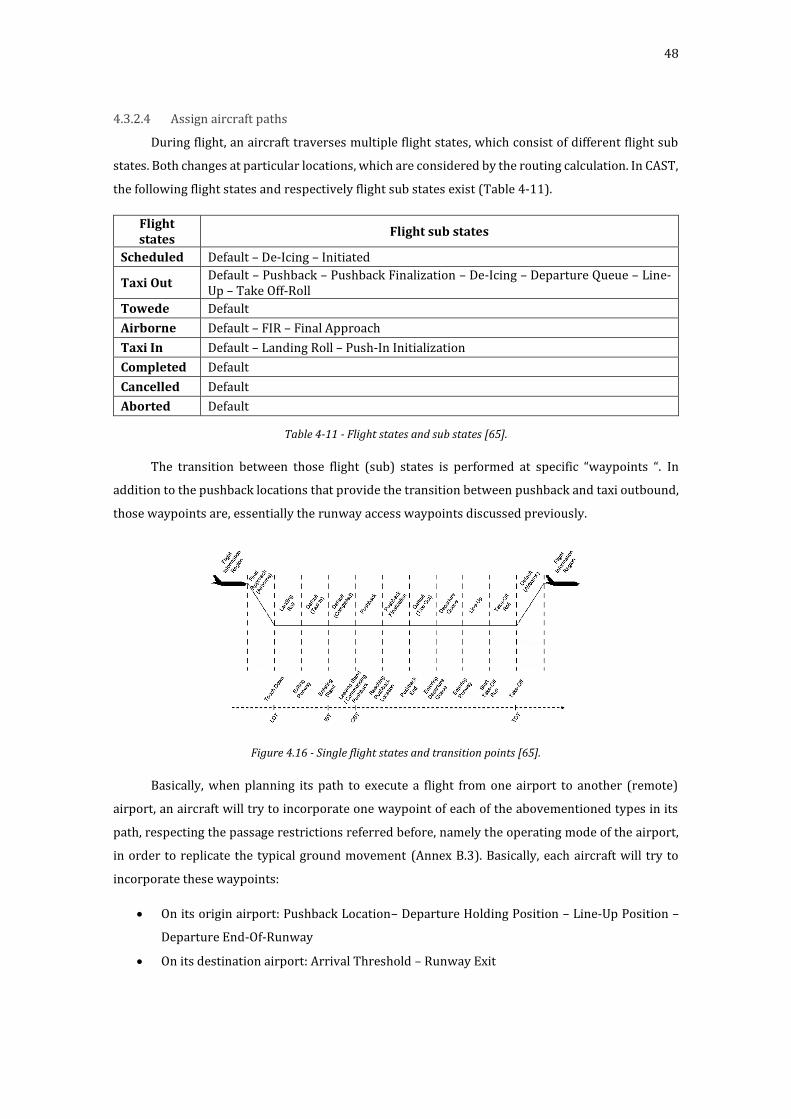
48

4.3.2.4 Assign aircraft paths

During flight, an aircraft traverses multiple flight states, which consist of different flight sub

states. Both changes at particular locations, which are considered by the routing calculation. In CAST,

the following flight states and respectively flight sub states exist (Table 4-11).

Flight states

Flight sub states

Scheduled Default – De-Icing – Initiated

Taxi Out Default – Pushback – Pushback Finalization – De-Icing – Departure Queue – Line-Up – Take Off-Roll

Towede Default

Airborne Default – FIR – Final Approach

Taxi In Default – Landing Roll – Push-In Initialization

Completed Default

Cancelled Default

Aborted Default

Table 4-11 - Flight states and sub states [65].

The transition between those flight (sub) states is performed at specific “waypoints “. In

addition to the pushback locations that provide the transition between pushback and taxi outbound,

those waypoints are, essentially the runway access waypoints discussed previously.

Figure 4.16 - Single flight states and transition points [65].

Basically, when planning its path to execute a flight from one airport to another (remote)

airport, an aircraft will try to incorporate one waypoint of each of the abovementioned types in its

path, respecting the passage restrictions referred before, namely the operating mode of the airport,

in order to replicate the typical ground movement (Annex B.3). Basically, each aircraft will try to

incorporate these waypoints:

On its origin airport: Pushback Location– Departure Holding Position – Line-Up Position –

Departure End-Of-Runway

On its destination airport: Arrival Threshold – Runway Exit

49

4.3.3 Model Initialization

4.3.3.1 Generating Traffic

There are two options to generate flights within CAST:

1. Importing a Flight Schedule

One of the main features of CAST is its ability to generate a schedule-based traffic flow. This

has the direct advantage of adding realism to the simulation. By importing a flight schedule one can

generate aircraft movements according to any preferences as well as, and most importantly, test the

model by importing a previous flight schedule and use it to serve as a model validation.

The flight schedule must consist of several rows and columns. Each row represents a single

aircraft movement (flight), while the columns reflect the properties of these movements. CAST uses

the CSV (comma separated values) format for importing and exporting the flight schedule. Every

imported flight schedule must have these mandatory entries: ReferenceTimestamp [Date/Time];

AircraftType [String]; RemoteAPT [String]; RemoteStand [String]; FlightDirection [Enumeration];

FlightNumber [String]; AirlineCode [String]; Registration [String] and LocalStand [String].

Although very useful, importing a flight schedule can become an inadequate method when the

user wants to test in a quick and easy way several flights conditions and different aircraft stand

allocation scenarios. This can turn out to be a problem when there is the need to test in a time-

efficient way, the airport’s maximum capacity. When that is the case, the need to define specific flight

characteristics, like a precise hour of arrival or departure, is overtaken by the need to run a large

number of tests with increasing flight demand, while ensuring that there are no big irregularities in

each run. Besides, in order to use this method, several historical detailed flight schedules are needed,

which can be difficult to obtain for academic purposes. That is exactly the case of this study and that

is why another object named “Traffic Flow Generator”, explained next, is used.

2. Traffic Flow Generator

CAST also allows the generation of flights according to user-defined rules. As mentioned

before, this can be done with Traffic Flow Generator (TFG). It is used for evaluating a network and

also for other types of analyses, as it works independently of any flight schedule.

TFG alone simply generates a continuous traffic flow from the pre-defined stand source(s) to

the pre-defined stand destination(s). In order to do that, first, one aircraft is chosen as the prototype

aircraft. Secondly, one should define sources and destinations for the traffic flow. As in CAST Aircraft

flight movements are always performed from stand to stand, stands are the sources and destinations

of all traffic. Once the TFG has at least one prototype, source and destination, it will generate a

continuous traffic flow from one of its sources to one of its destinations using one of its prototypes.

To get a more realistic aircraft traffic it is possible to adjust the probabilities of using any source,

destination and prototype or install two TFGs, one for outbound and one for inbound traffic.

50

TFG, together with two other objects, can generate a flight in every pre-defined time-step

during the simulation. Those objects are called Network Sector Analyser (NSA)and Progressor.

The NSA facilitates the local analysis of traffic flows by creating a sector defined by other

objects called Sector Transitions, which serve as entries or exits. The NSA detects all vehicles in the

area of interest, their time in the sector as well as their entry and exit. Following one can connect the

respective NSA, as well as the TFG, with a Progressor. A Progressor is an object which has an

evaluation unit that is evaluated in every time step. Therefore, one can use it to evaluate in every time

step how many aircraft are in the NSA in order to trigger whether aircraft should be generated by the

TFG or not. The maximum time-step allowed during the simulations was 1 second, which means that

the test is performed at least every second. Then, one should test this system with different values to

make sure that there are always enough aircraft in the sector without having an unacceptable queue

at the exiting transition of that sector.

In this study, two TFGs were used. For the outbound traffic generator all local stands were

used as sources and the single stand on the remote airport as destination. The opposite was done for

the inbound traffic generator. In addition, one NSA is created starting at the remote airport and

ending at the transition representing the final approach for inbound traffic, and another NSA is

created for outbound traffic using the aircraft stands as entries and the departure end of runway

transition as the single exit for the sector. The aircraft prototypes used were the Aibus A330-300,

Airbus A320-200 and Cessna Citation Mustang 510 for the Heavy, Medium and Light wake turbulence

category, respectively (Annex C.1).

With the aim of generating typical daily traffic in each simulation, there is also the need to

replicate the hourly peaks usually observed. In order to do that, the traffic generation process

differentiate periods of time in which the maximum number of aircraft allowed inside the NSAs is

greater. Those periods correspond to the previous mentioned: 0800-0900 UTC, 1400-1500 UTC and

2000-2100 UTC. Figure 4.17 represents the Progressor method. 𝑋1 and 𝑌1 variables correspond to

the of maximum number of aircraft allowed in the approach and maneuvering area sector,

respectively, during the morning and afternoon peak hours. 𝑋3 and 𝑌3 represent the maximum values

from 1400-1500 UTC. Finally, 𝑋2 and 𝑌2 correspond to the maximum aircraft permitted during the

rest of the day (0600-0800 UTC and 2100-2200 UTC). The values given to these variables were tested

until the movements generated would resemble to the typical daily traffic of LPPT and when it was

reasonable to assume the continuous generation of traffic during the traffic peaks (to test both

Ultimate and Practical Capacity). After testing all combinations possible with range of values from 1-

10 for each variable, the best values found to reproduce the typical high demand traffic were 3 for 𝑋1

and 𝑌1, 2 for 𝑋2 and 𝑌2, and 1 for 𝑋3 and 𝑌3.

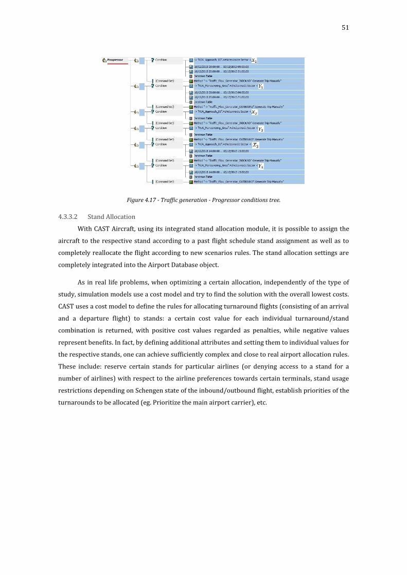
51

Figure 4.17 - Traffic generation - Progressor conditions tree.

4.3.3.2 Stand Allocation

With CAST Aircraft, using its integrated stand allocation module, it is possible to assign the

aircraft to the respective stand according to a past flight schedule stand assignment as well as to

completely reallocate the flight according to new scenarios rules. The stand allocation settings are

completely integrated into the Airport Database object.

As in real life problems, when optimizing a certain allocation, independently of the type of

study, simulation models use a cost model and try to find the solution with the overall lowest costs.

CAST uses a cost model to define the rules for allocating turnaround flights (consisting of an arrival

and a departure flight) to stands: a certain cost value for each individual turnaround/stand

combination is returned, with positive cost values regarded as penalties, while negative values

represent benefits. In fact, by defining additional attributes and setting them to individual values for

the respective stands, one can achieve sufficiently complex and close to real airport allocation rules.

These include: reserve certain stands for particular airlines (or denying access to a stand for a

number of airlines) with respect to the airline preferences towards certain terminals, stand usage

restrictions depending on Schengen state of the inbound/outbound flight, establish priorities of the

turnarounds to be allocated (eg. Prioritize the main airport carrier), etc.

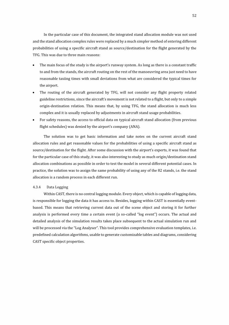
52

In the particular case of this document, the integrated stand allocation module was not used

and the stand allocation complex rules were replaced by a much simpler method of entering different

probabilities of using a specific aircraft stand as source/destination for the flight generated by the

TFG. This was due to three main reasons:

The main focus of the study is the airport’s runway system. As long as there is a constant traffic

to and from the stands, the aircraft routing on the rest of the manoeuvring area just need to have

reasonable taxiing times with small deviations from what are considered the typical times for

the airport.

The routing of the aircraft generated by TFG, will not consider any flight property related

guideline restrictions, since the aircraft's movement is not related to a flight, but only to a simple

origin-destination relation. This means that, by using TFG, the stand allocation is much less

complex and it is usually replaced by adjustments in aircraft stand usage probabilities.

For safety reasons, the access to official data on typical aircraft stand allocation (from previous

flight schedules) was denied by the airport’s company (ANA).

The solution was to get basic information and take notes on the current aircraft stand

allocation rules and get reasonable values for the probabilities of using a specific aircraft stand as

source/destination for the flight. After some discussion with the airport’s experts, it was found that

for the particular case of this study, it was also interesting to study as much origin/destination stand

allocation combinations as possible in order to test the model in several different potential cases. In

practice, the solution was to assign the same probability of using any of the 82 stands, i.e. the stand

allocation is a random process in each different run.

4.3.4 Data Logging

Within CAST, there is no central logging module. Every object, which is capable of logging data,

is responsible for logging the data it has access to. Besides, logging within CAST is essentially event-

based. This means that retrieving current data out of the scene object and storing it for further

analysis is performed every time a certain event (a so-called “log event”) occurs. The actual and

detailed analysis of the simulation results takes place subsequent to the actual simulation run and

will be processed via the “Log Analyser”. This tool provides comprehensive evaluation templates, i.e.

predefined calculation algorithms, usable to generate customizable tables and diagrams, considering

CAST specific object properties.

53

The objects used to directly aggregate and analyze data were:

Network Sector Analyser: as mentioned before, the sector to analyse is defined by sector

transitions, which serve as entries or exits. This way, this object detects all vehicles in the area

of interest, their time in the sector as well as their entry and exit. It is used in the RWY system

for analysis of specified areas concerning daily RWY throughput using 10 minute steps:

o Number of Arrival, departure and total movements;

o Number of Movements per aircraft type;

o Number of Movements per RWY exit;

o ROTS.

Ground Controller: as referred before, the Ground Controller is the NSA equivalent for the entire

infrastructure on the ground. This way, it is used in a similar way as the RWY NSA, to calculate:

o Average taxi-times;

o TOP 90 percentile analysis;

o Maximum taxi-times.

Queue Detector: determines the number of aircraft in a queue, the queue length and the queuing

times. During the simulation, the Queue Detector also draws a frame around all aircraft it has

detected to be in the queue, helping to visualise the main taxiway bottlenecks (Figure 4.18).

Based on the values obtained from the DHP it is used to calculate:

o Average dwell times;

o TOP 90 percentile analysis;

o Maximum dwell times.

Figure 4.18 - Queue Detector frame [65].

The only data that is not retrieved directly from the Log Analyzer is related with the mix of

operations observed during the simulations. As logging within CAST is basically event-based, in order

to obtain that values, a simple test was performed with the data retrieved from the TFG: using 1-

minute step (the smallest possible), the traffic per dispatching center (remote stand for arrivals and

local stands for departures) was calculated and every time a difference in the traffic between two

time intervals is verified, it is assumed that there was an arrival or departure. This way, with the

correspondent sequence, it is possible to make a rough estimate on the proportion of sequences

during the simulation. Consequently, the ADA sequence is divided into DA and AD sequences.

54

Output Data Evaluation

The first thing to do when evaluating a model is to determine if it is an acceptable

representation of the real system. For that purpose, the flights demand, mix of operations, taxi-times,

ROTs and delays are compared to what is considered typical and there is a basic deviation (from

target) analysis for those outputs. Since there is randomness while using probabilities in some inputs,

the next step is to perform several replications (𝑛) to deal with the stochastic variations, and to

precisely estimate measurements uncertainty and outputs statistical significance.

The main focus is the runway capacity of each scenario. In that case, for the daily number of

movements mean observed in each sample, for which an estimated value, µ̄, and an estimate of the

standard deviation, 𝑠, is calculated, one can report confidence intervals by means of parametric

descriptive statistics analysis. For that reason, one should first explore the normality of the output

data-set before deciding the use of parametric analysis.

To test the assumption of normality, various measures and tests can be applied. They fall into

two broad categories: graphical and statistical. In terms of statistical methods, a 2011 study

concluded that Shapiro–Wilk has the best power for a given significance, followed closely by

Anderson–Darling when comparing the Shapiro–Wilk, Kolmogorov–Smirnov, Lilliefors, and

Anderson–Darling tests [76]. For that reason, Shapiro-Wilk’s test is performed for every sample,

using an algorithm by Royston [77]. Assuming that the sample has n elements, the algorithm follows

these steps [78]:

1. Sort the data in ascending order 𝑥1 ≤ … ≤ 𝑥𝑛

2. Define the values 𝑚1, … , 𝑚𝑛 by3:

𝑚𝑖 = 𝑁𝑂𝑅𝑀𝑆𝐼𝑁𝑉 (𝑖 − .375

𝑛 + .25)

(4-1)

3. Assuming 𝑀 = [𝑚𝑖], the 𝑛 × 1 column vector whose elements are these 𝑚𝑖 , then:

𝑚 = 𝑀 ⋅ 𝑀 = 𝑀𝑇𝑀 = ∑ 𝑚𝑖2

𝑛

𝑖=1

(4-2)

4. Define the coefficients 𝑎1, … , 𝑎𝑛:

𝑎𝑛 = −2.706056𝑢5 + 4.434685𝑢4 − 2.701190𝑢3 − 0.147981𝑢2 + 0.221157𝑢

+ 𝑚𝑛𝑚−0.5

(4-3)

3 𝑁𝑂𝑅𝑀𝑆𝐼𝑁𝑉(𝑥) = Inverse of the standard normal cumulative distribution with probability of

x

55

𝑎𝑛−1 = −3.582633𝑢5 + 5682633𝑢4 − 1.752461𝑢3 − 0.293762𝑢2 + 0.042981𝑢

+ 𝑚𝑛−1𝑚−0.5

(4-4)

𝑎𝑖 = 𝑚𝑖 /√(𝜖) for 2 < 𝑖 < 𝑛 − 1

(4-5)

𝑎2 = −𝑎𝑛−1 𝑎1 = −𝑎𝑛 (4-6)

Where:

𝑢 = 1/√(𝑛)

𝜖 =𝑚 − 2𝑚𝑛

2 − 2𝑚𝑛−12

1 − 2𝑎𝑛2 − 2𝑎𝑛−1

2

Assuming 𝐴 = [𝑎𝑖] is the 𝑛 × 1 column vector whose elements are 𝑎𝑖 = −𝑎𝑛 − 𝑖 + 1 for all i:

1 = 𝐴 ⋅ 𝐴 = 𝐴𝑇𝐴 = ∑ 𝑎𝑖2

𝑛

𝑖=1

(4-7)

5. Define the W statistic:

𝑊 =(∑ 𝑎𝑖𝑥𝑖

𝑛𝑖=1 )2

(∑ 𝑥𝑖 − �̄�𝑛𝑖=1 )2

(4-8)

This way W equals the square of the correlation coefficient between 𝑎1, … , 𝑎𝑛 and 𝑥1, … , 𝑥𝑛.

Thus the values of W are always between 0 and 1. One may also assume that for values of 𝑛 between

12 and 5,000 the statistic 𝑙𝑛 (1 − 𝑊) is approximately normally distributed with the following mean

and standard deviation:

µ = 0.0038915 (ln 𝑛)3 − 0.083751(ln 𝑛)2 − 0.31082 ln 𝑛 − 1.5861

(4-9)

𝜎 = 𝑒0.0030302(ln 𝑛)2−0.082676 ln 𝑛−0.4803

(4-10)

6. Finally, test the statistic using the standard normal distribution:

𝑧 =ln(1 − 𝑊) − µ

𝜎

(4-11)

56

The test should not be significant to meet the assumption of normality, i.e. the p-value must

be greater than the significance level, 𝛼, which, by definition, corresponds to the probability of

rejecting the null hypothesis when the null hypothesis is true. In this case, the hypotheses used are:

𝐻0: The sample data are not significantly different than a normal population.

𝐻𝑎: The sample data are significantly different than a normal population.

Since the test is biased by sample size, the test may be statistically significant from a normal

distribution in any large samples. Therefore, a Q–Q plot is usually required for verification in addition

to the test. For that reason, Q-Q plots for each sample size are also generated in order to better

visualize the samples distributions and compare them to the standard normal distribution - Normal

Probability Plots 𝑁(0,1).

As the observations are independent and the sampling is random, if the errors in the daily

movements have a normal probability distribution, then the probability distribution for the error in

the sample mean, normalized by the standard error in the sample average, is the t-distribution. The

t-statistic of interest is that which bounds a chosen level of probability, 1 - α, for the t-distribution

with n - 1 degrees of freedom. Then, one can conclude that there is a 1 - α probability that the

Confidence Interval (CI) contains the true value of µ̄. In this case, the value used for 𝛼 was 0.05 (95%

confidence). The 1-α CI for µ̄ is:

𝐶𝐼 = µ̄ ± 𝑤 = µ̄ ± 𝑡𝑛−1;𝛼/2𝑠µ̄ (4-12)

Where: 𝑤 = Confidence Interval half-width 𝑡𝑛−1;𝛼/2 = t-statistic corresponding to the α/2 probability (representing one side of a symmetric

two-sided interval)

𝑠µ̄ =𝑠

√𝑛 = standard error of the mean

Essentially, in order to ensure mean statistical significance for the daily movements, the

number of replications is increased in increments of 10 until the assumption of normality for the

sample data is acceptable and w is below 1. The rest of the data is examined according to the average

of the total replications (per scenario), with the exception of ROTs, as they do not change from

replication to replication (the acceleration profiles remains the same for all aircraft).

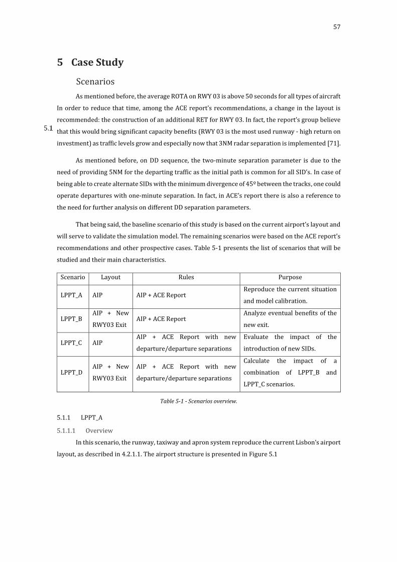
57

5 Case Study

Scenarios

As mentioned before, the average ROTA on RWY 03 is above 50 seconds for all types of aircraft

In order to reduce that time, among the ACE report’s recommendations, a change in the layout is

recommended: the construction of an additional RET for RWY 03. In fact, the report’s group believe

that this would bring significant capacity benefits (RWY 03 is the most used runway - high return on

investment) as traffic levels grow and especially now that 3NM radar separation is implemented [71].

As mentioned before, on DD sequence, the two-minute separation parameter is due to the

need of providing 5NM for the departing traffic as the initial path is common for all SID’s. In case of

being able to create alternate SIDs with the minimum divergence of 45º between the tracks, one could

operate departures with one-minute separation. In fact, in ACE’s report there is also a reference to

the need for further analysis on different DD separation parameters.

That being said, the baseline scenario of this study is based on the current airport’s layout and

will serve to validate the simulation model. The remaining scenarios were based on the ACE report’s

recommendations and other prospective cases. Table 5-1 presents the list of scenarios that will be

studied and their main characteristics.

Scenario Layout Rules Purpose

LPPT_A AIP AIP + ACE Report Reproduce the current situation

and model calibration.

LPPT_B AIP + New

RWY03 Exit AIP + ACE Report

Analyze eventual benefits of the

new exit.

LPPT_C AIP AIP + ACE Report with new

departure/departure separations

Evaluate the impact of the

introduction of new SIDs.

LPPT_D AIP + New

RWY03 Exit

AIP + ACE Report with new

departure/departure separations

Calculate the impact of a

combination of LPPT_B and

LPPT_C scenarios.

Table 5-1 - Scenarios overview.

5.1.1 LPPT_A

5.1.1.1 Overview

In this scenario, the runway, taxiway and apron system reproduce the current Lisbon’s airport

layout, as described in 4.2.1.1. The airport structure is presented in Figure 5.1

58

Figure 5.1 - CAST model of current LPPT layout.

As mentioned before, the aircraft separations are the current wake-turbulence minima,

obtained from the ACE’s report:

Arrival/Arrival:

Following Aircraft

Light Medium Heavy

Leading

Aircraft

Light 5 NM 5 NM 5 NM

Medium 5 NM 5 NM 5 NM

Heavy 6 NM 5 NM 5 NM

Table 5-2 - Arrival aircraft separation minima.

Arrival/Departure/Arrival: 6NM.

Departure/Departure: 2minutes.

Based on the maximum speeds allowed published in the LPPT EUROCONTROL Airport Public

Corner [3] and with some advice from the airport experts, it was decided to create a terminal

approach airspace starting at 8NM from RWY 03 threshold, divided in four segments of 2NM each.

The maximum speeds allowed were 180 knots (8NM - 6NM), 160 knots (6NM - 4NM), 140 knots

(4NM - 2NM) and 120 knots (2NM - RWY threshold).

Figure 5.2 - Terminal approach and airport model overview.

59

The aircraft fleet mix (Table 5-3) and the exits usage distribution (Table 5-4) are based on the

ACE report with some minor adjustments. Based on those values, the total use of the exits should be

around 60% for HN, 30% for RWY 17, 8.7% for S1 and 1.3% for U5.

Flight Direction Light Medium Heavy

Inbound 10% 80% 10%

Outbound 4% 95% 1%

Table 5-3 - Aircraft fleet mix used as inputs during the simulations, by flight direction.

Exits usage distribution (%)

Wake-turbulence category RWY 17 S1 HN U5

Light 100 0 0 0

Medium 25 9 65 1

Heavy 0 15 80 5

Table 5-4 - Exits usage distribution for LPPT_A and LPPT_B scenarios.

5.1.1.2 Results

After 40 replications, the p-value obtained with the WS test was 0,24 which is greater than the

𝛼 (0.05) meaning that the assumption of the sample normality distribution is not rejected, confirmed

by the observation of the Q-Q plot (Figure 5.3).

Figure 5.3- LPPT_A Normal Probability Plot - 40 Replications Sample.

The descriptive analysis for the daily movements data is presented in Table 5-5. The CI for the

sample total daily movements mean is approximately [409 ± 0.95], which means that is reasonable

to conclude that for the reference scenario the daily average would be around 408 to 410 movements,

with all the assumptions made before.

60

LPPT_ A Daily Movements - 40 Replications Sample Mean 409

Standard Error of the Mean 0,47 Median 410 Mode 410

Standard Deviation 2,96 Sample Variance 8,77

Kurtosis -0,37 Skewness -0,26

Range 12 Minimum 403 Maximum 415

Confidence Level (95,0%) 0,95

Table 5-5 - LPPT_A descriptive statistics - 40 replications.

Table 5-6 presents the results for ROTs for arrival (per exit) and for departure. The results for

ROTAs are close to the observed in ACE’s report for HN and RWY 17 exits: 2 seconds difference in

both cases. S1 exit ROTA is equal to the observed in the exercise. In the case of U5 the 62 seconds

result was found suitable according to the typical values. The ROTD corresponds to the interval

between the line-up position and the end of the runway, i.e. it is the sum of the ATC take-off clearance

time (TOCD), the flight crew reaction to line-up clearance (FRLC) and the take-off roll time (TOFT),

assuming, in this case, that both TOCD and FRLC are included in the TOFT. There is a difference of 3.2

seconds between the model’s ROTD and the observed 49.8 seconds (4.1 + 14.3 + 31.4) total departure

time after the aircraft has been lined up. Considering these distributions and the ROTAs obtained for

each exit, the average ROTA for this scenario is 54.3 seconds, which is very close to the historical

value of 54.1 seconds.

RWY 03 ROTs per exit - LPPT_A and LPPT_C scenarios

RWY 03 Exit HN S1 RWY 17 U5 Departure End of Runway

ROT (seconds) 54 59 53 62 53

Table 5-6 - RWY3 ROTs per exit for LPPT_A and LPPT_c scenarios.

LPPT_A Average Arrival Exit Distribution - 40 Replications Sample

HN (%) RWY17 (%) S1 (%) U5 (%)

62,0 27,8 8,8 1,4

Table 5-7 - LPPT_A Average Arrival Exit Distribution - 40 Replications Sample.

The average aircraft fleet mix for the 40 sample is presented in Table 5-8. As expected, most

aircraft are medium type followed by the light and the heavy, which means that most approach

movements are separated 5NM from each other in the approach segment.

LPPT_A Aircraft Fleet Mix - 40 Replications Sample

Light (%) Medium (%) Heavy (%)

7,0 87,3 5,7

Table 5-8 - LPPT_A Aircraft Fleet Mix - 40 Replications Sample.

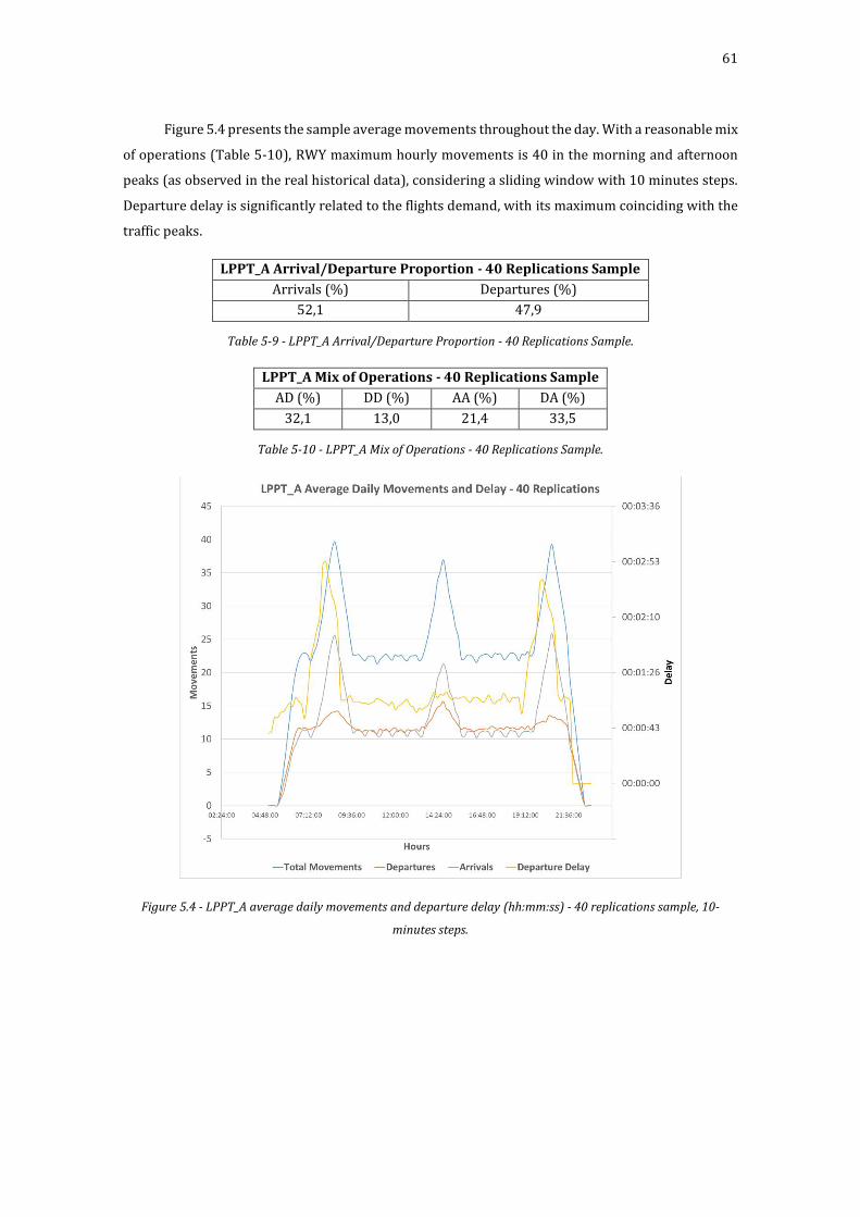
61

Figure 5.4 presents the sample average movements throughout the day. With a reasonable mix

of operations (Table 5-10), RWY maximum hourly movements is 40 in the morning and afternoon

peaks (as observed in the real historical data), considering a sliding window with 10 minutes steps.

Departure delay is significantly related to the flights demand, with its maximum coinciding with the

traffic peaks.

LPPT_A Arrival/Departure Proportion - 40 Replications Sample

Arrivals (%) Departures (%)

52,1 47,9

Table 5-9 - LPPT_A Arrival/Departure Proportion - 40 Replications Sample.

LPPT_A Mix of Operations - 40 Replications Sample

AD (%) DD (%) AA (%) DA (%)

32,1 13,0 21,4 33,5

Table 5-10 - LPPT_A Mix of Operations - 40 Replications Sample.

Figure 5.4 - LPPT_A average daily movements and departure delay (hh:mm:ss) - 40 replications sample, 10-

minutes steps.

62

5.1.2 LPPT_B

5.1.2.1 Overview

In Scenario LPPT_B the layout includes the new rapid exit for RWY 03. The new exit is identical

to the existent one (HN), i.e. it has a standard design in accordance with the specifications given in

ICAO Aerodrome Design Manual for airport code number 3 and 4 (Annex A). As mentioned before,

using the three segment method one can calculate the total landing distance for aircraft of category

A/B and C/D. Assuming threshold speed of 105 knots for aircraft category A/B and 120 knots for

C/D, and assuming a deceleration rate of −1.5 𝑚/𝑠2 the total distances are given by:

Aircraft category A and B:

o S1 = 250 m.

o 𝑆2 = 5 × (𝑉𝑡ℎ − 10) = 5× (105 − 10) = 475 𝑚

o 𝑆3 =𝑉𝑏𝑎

2 −𝑉𝑒𝑥2

2𝑎=

((105−15) ×0.51 )2

−( 30×0.51 )2

2∗1.5≃ 624.24 𝑚

o Total distance = S1 + S2 + S3 = 1349.24 m

Aircraft category C and D:

o S1 = 450 m.

o 𝑆2 = 5 × (𝑉𝑡ℎ − 10) = 5× (120 − 10) = 550 𝑚

o 𝑆3 =𝑉𝑏𝑎

2 −𝑉𝑒𝑥2

2𝑎=

((120−15) ×0.51 )2

−( 30×0.51 )2

2∗1.5≃ 877.84 𝑚

o Total distance = S1 + S2 + S3 = 1877.84 m

Assuming that the new rapid exit is mainly for aircraft approaching with threshold speed of

between 110 knots to 120 knots (between category B and C) the ideal distance would be between

the correspondent ideal distances for each category, i.e. between 1349.24m and 1877.84m. Another

important analysis has to do with the need for a smooth turn after exiting the runway. As said before,

ICAO recommends a straight tangent section after the turnoff curve to allow exiting aircraft to come

to a full stop clear of the intersecting taxiway when the intersection is 30°. Assuming deceleration

rates of 1.52 𝑚/s2 along the straight section, this tangent distance should be not less than 75 m for

aerodrome code number 3 or 4. Despite most aircraft arriving at LPPT belong to category C, after a

series of pilot tests, it was decided to place the new exit at 1500 m from RWY03 threshold.

63

Figure 5.5 - CAST model for LPPT’s layout with the new RET.

The inputs are the same as LPPT_A except the exits usage distribution that now has to take

into account the new exit, from now on named “HG”. It was decided to assign all light aircraft to the

new exit. Considering the airport expert’s opinion, and assuming that the new rapid exit would be

used by a smaller amount of aircraft than the already existing one, 60% and 30% of medium and

heavy aircraft, are distributed by the new exit, respectively. The aircraft distribution for the rest of

the exits followed the baseline scenario proportion. Assuming the same aircraft fleet mix used in

LPPT_A scenario, the total use of the exits should be around 61% for HG, 26.4% for HN, 8% for RWY

17, 3.93% for S1 and 0.67% for U5.

Exits usage distribution (%)

RWY 17 HG S1 HN U5

Light 0 100 0 0 0

Medium 10 60 3.6 26 0.4

Heavy 0 30 10.5 56 3.5

Table 5-11 - Exits usage distribution for LPPT_B and LPPT_D scenarios.

5.1.2.2 Results

In this case, the number of replications required to accept the normality of the sample mean

was 30 replications. The p-value obtained with the WS test was 0,0533 (>0.05). The Q-Q plot is

presented in Figure 5.6.

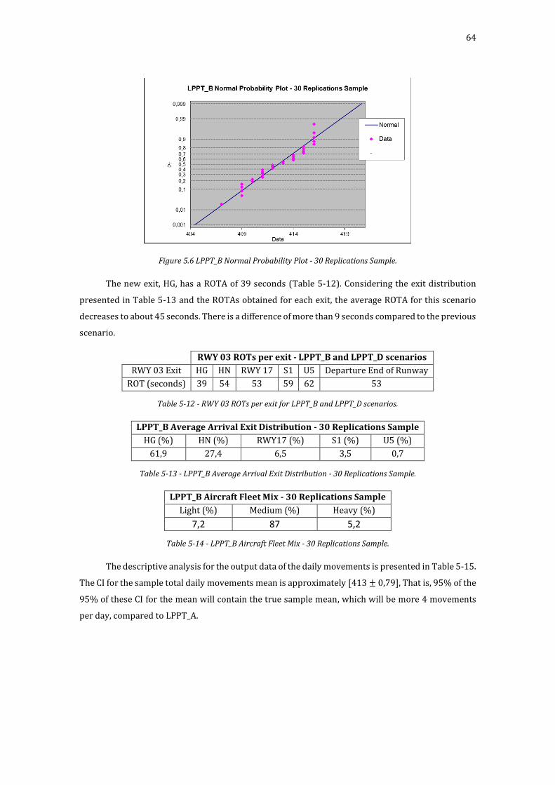
64

Figure 5.6 LPPT_B Normal Probability Plot - 30 Replications Sample.

The new exit, HG, has a ROTA of 39 seconds (Table 5-12). Considering the exit distribution

presented in Table 5-13 and the ROTAs obtained for each exit, the average ROTA for this scenario

decreases to about 45 seconds. There is a difference of more than 9 seconds compared to the previous

scenario.

RWY 03 ROTs per exit - LPPT_B and LPPT_D scenarios

RWY 03 Exit HG HN RWY 17 S1 U5 Departure End of Runway

ROT (seconds) 39 54 53 59 62 53

Table 5-12 - RWY 03 ROTs per exit for LPPT_B and LPPT_D scenarios.

LPPT_B Average Arrival Exit Distribution - 30 Replications Sample

HG (%) HN (%) RWY17 (%) S1 (%) U5 (%)

61,9 27,4 6,5 3,5 0,7

Table 5-13 - LPPT_B Average Arrival Exit Distribution - 30 Replications Sample.

LPPT_B Aircraft Fleet Mix - 30 Replications Sample

Light (%) Medium (%) Heavy (%)

7,2 87 5,2

Table 5-14 - LPPT_B Aircraft Fleet Mix - 30 Replications Sample.

The descriptive analysis for the output data of the daily movements is presented in Table 5-15.

The CI for the sample total daily movements mean is approximately [413 ± 0,79], That is, 95% of the

95% of these CI for the mean will contain the true sample mean, which will be more 4 movements

per day, compared to LPPT_A.

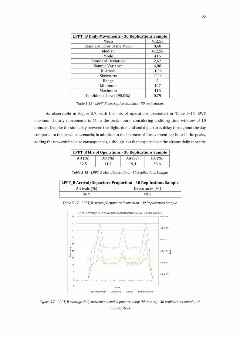
65

LPPT_ B Daily Movements - 30 Replications Sample Mean 412,53

Standard Error of the Mean 0,48 Median 412,50 Mode 416

Standard Deviation 2,62 Sample Variance 6,88

Kurtosis -1,04 Skewness -0,24

Range 9 Minimum 407 Maximum 416

Confidence Level (95,0%) 0,79

Table 5-15 - LPPT_B descriptive statistics - 30 replications.

As observable in Figure 5.7, with the mix of operations presented in Table 5-16, RWY

maximum hourly movements is 41 in the peak hours, considering a sliding time window of 10

minutes. Despite the similarity between the flights demand and departures delay throughout the day

compared to the previous scenario, in addition to the increase of 1 movement per hour in the peaks,

adding the new exit had also consequences, although less than expected, on the airport daily capacity.

LPPT_B Mix of Operations - 30 Replications Sample

AD (%) DD (%) AA (%) DA (%)

32,5 11,4 19,4 33,6

Table 5-16 - LPPT_B Mix of Operations - 30 Replications Sample.

LPPT_B Arrival/Departure Proportion - 30 Replications Sample

Arrivals (%) Departures (%)

50.9 49.1

Table 5-17 - LPPT_B Arrival/Departure Proportion - 30 Replications Sample.

Figure 5.7 - LPPT_B average daily movements and departure delay (hh:mm:ss) - 30 replications sample, 10-

minutes steps.

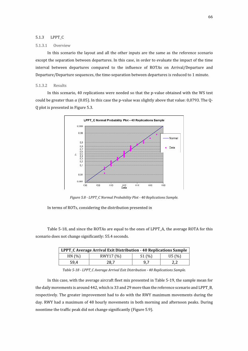
66

5.1.3 LPPT_C

5.1.3.1 Overview

In this scenario the layout and all the other inputs are the same as the reference scenario

except the separation between departures. In this case, in order to evaluate the impact of the time

interval between departures compared to the influence of ROTAs on Arrival/Departure and

Departure/Departure sequences, the time-separation between departures is reduced to 1 minute.

5.1.3.2 Results

In this scenario, 40 replications were needed so that the p-value obtained with the WS test

could be greater than 𝛼 (0.05). In this case the p-value was slightly above that value: 0,0793. The Q-

Q plot is presented in Figure 5.3.

Figure 5.8 - LPPT_C Normal Probability Plot - 40 Replications Sample.

In terms of ROTs, considering the distribution presented in

Table 5-18, and since the ROTAs are equal to the ones of LPPT_A, the average ROTA for this

scenario does not change significantly: 55.4 seconds.

Table 5-18 - LPPT_C Average Arrival Exit Distribution - 40 Replications Sample.

In this case, with the average aircraft fleet mix presented in Table 5-19, the sample mean for

the daily movements is around 442, which is 33 and 29 more than the reference scenario and LPPT_B,

respectively. The greater improvement had to do with the RWY maximum movements during the

day. RWY had a maximum of 48 hourly movements in both morning and afternoon peaks. During

noontime the traffic peak did not change significantly (Figure 5.9).

LPPT_C Average Arrival Exit Distribution - 40 Replications Sample

LPPT_C Average Arrival Exit Distribution - 40 Replications Sample

HN (%) RWY17 (%) S1 (%) U5 (%)

59,4 28,7 9,7 2,2

67

LPPT_C Aircraft Fleet Mix - 40 Replications Sample

Light (%) Medium (%) Heavy (%)

5,9 88,8 5,4

Table 5-19 - LPPT_C Aircraft Fleet Mix - 40 Replications Sample.

LPPT_C Arrival/Departure Proportion - 40 Replications Sample

Arrivals (%) Departures (%)

48,5 51,5

Table 5-20 - LPPT_C Arrival/Departure Proportion - 40 Replications Sample.

LPPT_C Mix of Operations - 40 Replications Sample

AD (%) DD (%) AA (%) DA (%)

34,5 13,8 17,4 34,3

Table 5-21 - LPPT_C Mix of Operations - 40 Replications Sample.

LPPT_ C Daily Movements - 40 Replications Sample Mean 442

Standard Error of the Mean 0,30

Median 442

Mode 442

Standard Deviation 1,89

Sample Variance 3,58

Kurtosis 0,14

Skewness 0,47

Range 8,00

Minimum 439

Maximum 447

Confidence Level (95,0%) 0,61

Table 5-22 - LPPT_C descriptive statistics - 40 replications.

Figure 5.9 - LPPT_C average daily movements and departure delay (hh:mm:ss) - 40 replications sample, 10-

minutes steps.

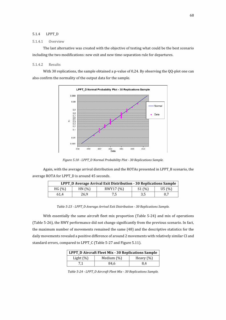
68

5.1.4 LPPT_D

5.1.4.1 Overview

The last alternative was created with the objective of testing what could be the best scenario

including the two modifications: new exit and new time-separation rule for departures.

5.1.4.2 Results

With 30 replications, the sample obtained a p-value of 0,24. By observing the QQ-plot one can

also confirm the normality of the output data for the sample.

Figure 5.10 - LPPT_D Normal Probability Plot - 30 Replications Sample.

Again, with the average arrival distribution and the ROTAs presented in LPPT_B scenario, the

average ROTA for LPPT_D is around 45 seconds.

Table 5-23 - LPPT_D Average Arrival Exit Distribution - 30 Replications Sample.

With essentially the same aircraft fleet mix proportion (Table 5-24) and mix of operations

(Table 5-26), the RWY performance did not change significantly from the previous scenario. In fact,

the maximum number of movements remained the same (48) and the descriptive statistics for the

daily movements revealed a positive difference of around 2 movements with relatively similar CI and

standard errors, compared to LPPT_C (Table 5-27 and Figure 5.11).

LPPT_D Aircraft Fleet Mix - 30 Replications Sample

Light (%) Medium (%) Heavy (%)

7,1 84,6 8,4

Table 5-24 - LPPT_D Aircraft Fleet Mix - 30 Replications Sample.

LPPT_D Average Arrival Exit Distribution - 30 Replications Sample

LPPT_C Average Arrival Exit Distribution - 40 Replications Sample

HG (%) HN (%) RWY17 (%) S1 (%) U5 (%)

61,4 26,9 7,5 3,5 0,7

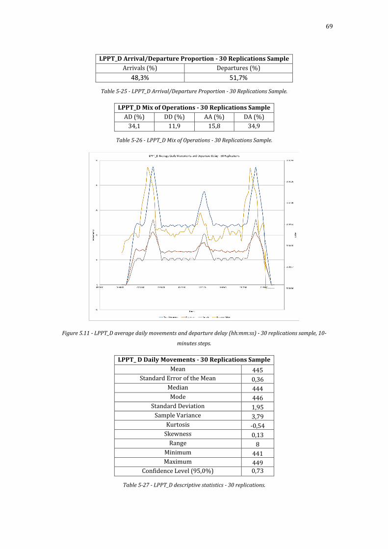
69

LPPT_D Arrival/Departure Proportion - 30 Replications Sample

Arrivals (%) Departures (%)

48,3% 51,7%

Table 5-25 - LPPT_D Arrival/Departure Proportion - 30 Replications Sample.

LPPT_D Mix of Operations - 30 Replications Sample

AD (%) DD (%) AA (%) DA (%)

34,1 11,9 15,8 34,9

Table 5-26 - LPPT_D Mix of Operations - 30 Replications Sample.

Figure 5.11 - LPPT_D average daily movements and departure delay (hh:mm:ss) - 30 replications sample, 10-

minutes steps.

LPPT_ D Daily Movements - 30 Replications Sample

Mean 445 Standard Error of the Mean 0,36

Median 444 Mode 446

Standard Deviation 1,95 Sample Variance 3,79

Kurtosis -0,54 Skewness 0,13

Range 8 Minimum 441 Maximum 449

Confidence Level (95,0%) 0,73

Table 5-27 - LPPT_D descriptive statistics - 30 replications.

70

Discussion

The reproduction and calibration of the reference scenario resulted in realistic simulations

with consistent performance data compared to the historical data. The visualization of the aircraft

movements and interaction during the simulations also contributed to confirm the reliability of the

model:

Correct pushback and parking maneuvering;

No excessive vehicle interaction or congestion problems were verified;

The airport’s operating mode was plainly respected (Annex B.3);

Realistic ROTs;

Realistic taxi-in and taxi-out times (Table 5-28);

Reasonable departure queue delay and lengths;

In what concerns ROTS, as discussed before, the results for the baseline scenario were

satisfactory will small deviations from the historical values. In terms of airside operations durations

and delay, the values presented in Table 5-28 correspond to the complete ground maneuvering, i.e.

for the outbound traffic the departure delay in queue and the delay during pushback are included in

those values, for example. The ROTs are also included in the taxiing durations for both directions.

The average durations found with the fast-time simulations were slightly below the historical values.

Two reasons may be responsible for these difference:

Speeds: In the fast-time simulations, only maximum fixed ground speeds for aircraft could

be used because the simulation did not allow momentary speed changes. This could be done,

for example, as in real world situations, depending on the current traffic congestion. In

practice, controllers can influence the speeds of aircraft with specific commands for each

flight, such as to expedite taxi or slow down. In addition, in the real world, the aircraft are

subjected to variations in their accelerations/velocities, which means that, in most cases, the

aircraft will not follow its path as quick as the airport taxiway layout and the aircraft

characteristics would allow.

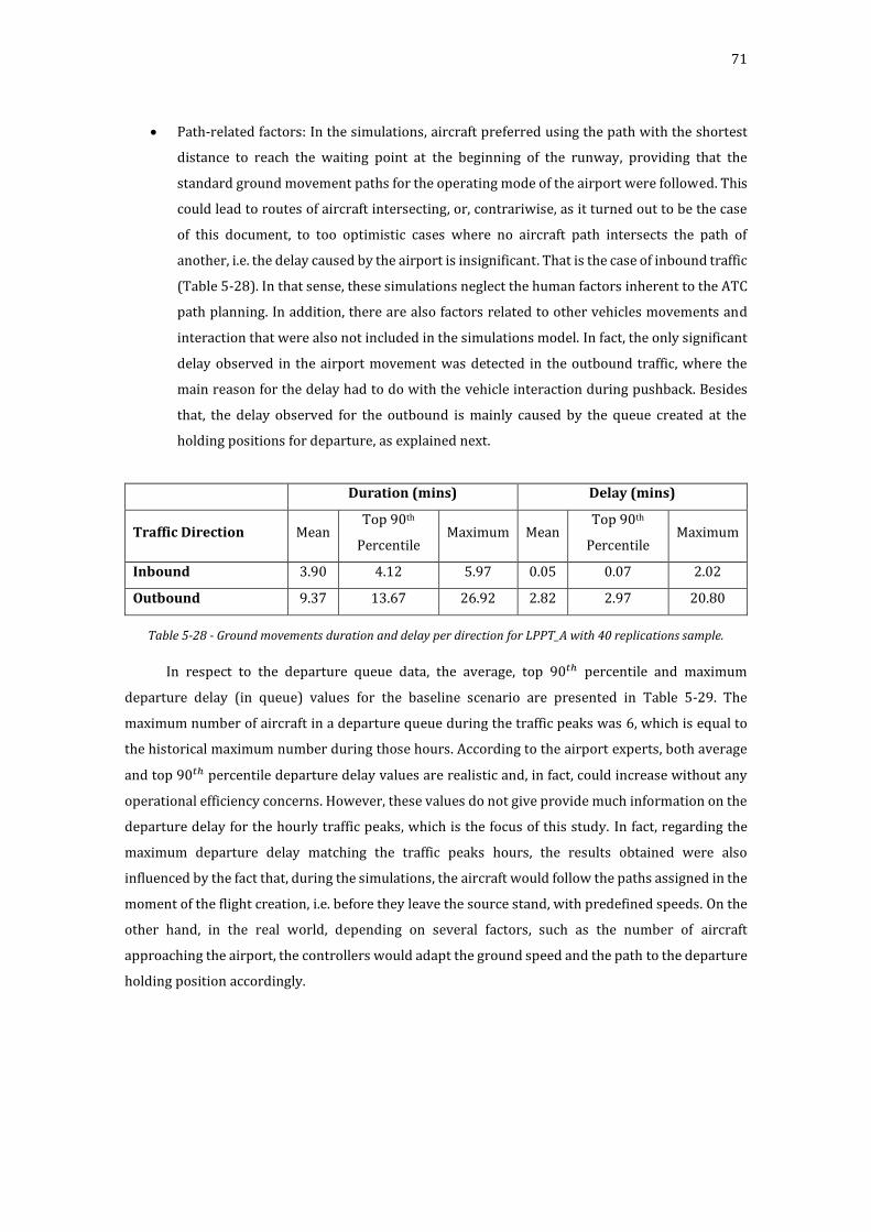
71

Path-related factors: In the simulations, aircraft preferred using the path with the shortest

distance to reach the waiting point at the beginning of the runway, providing that the

standard ground movement paths for the operating mode of the airport were followed. This

could lead to routes of aircraft intersecting, or, contrariwise, as it turned out to be the case

of this document, to too optimistic cases where no aircraft path intersects the path of

another, i.e. the delay caused by the airport is insignificant. That is the case of inbound traffic

(Table 5-28). In that sense, these simulations neglect the human factors inherent to the ATC

path planning. In addition, there are also factors related to other vehicles movements and

interaction that were also not included in the simulations model. In fact, the only significant

delay observed in the airport movement was detected in the outbound traffic, where the

main reason for the delay had to do with the vehicle interaction during pushback. Besides

that, the delay observed for the outbound is mainly caused by the queue created at the

holding positions for departure, as explained next.

Duration (mins) Delay (mins)

Traffic Direction Mean Top 90th

Percentile Maximum Mean

Top 90th

Percentile Maximum

Inbound 3.90 4.12 5.97 0.05 0.07 2.02

Outbound 9.37 13.67 26.92 2.82 2.97 20.80

Table 5-28 - Ground movements duration and delay per direction for LPPT_A with 40 replications sample.

In respect to the departure queue data, the average, top 90𝑡ℎ percentile and maximum

departure delay (in queue) values for the baseline scenario are presented in Table 5-29. The

maximum number of aircraft in a departure queue during the traffic peaks was 6, which is equal to

the historical maximum number during those hours. According to the airport experts, both average

and top 90𝑡ℎ percentile departure delay values are realistic and, in fact, could increase without any

operational efficiency concerns. However, these values do not give provide much information on the

departure delay for the hourly traffic peaks, which is the focus of this study. In fact, regarding the

maximum departure delay matching the traffic peaks hours, the results obtained were also

influenced by the fact that, during the simulations, the aircraft would follow the paths assigned in the

moment of the flight creation, i.e. before they leave the source stand, with predefined speeds. On the

other hand, in the real world, depending on several factors, such as the number of aircraft

approaching the airport, the controllers would adapt the ground speed and the path to the departure

holding position accordingly.

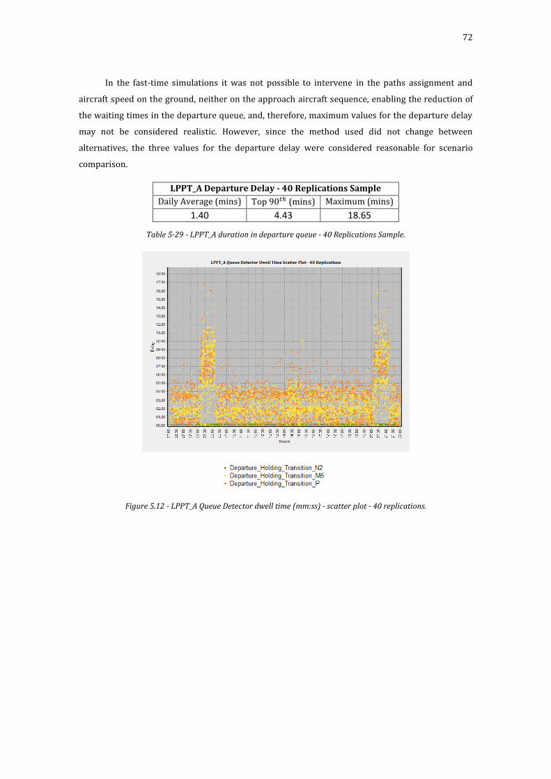
72

In the fast-time simulations it was not possible to intervene in the paths assignment and

aircraft speed on the ground, neither on the approach aircraft sequence, enabling the reduction of

the waiting times in the departure queue, and, therefore, maximum values for the departure delay

may not be considered realistic. However, since the method used did not change between

alternatives, the three values for the departure delay were considered reasonable for scenario

comparison.

LPPT_A Departure Delay - 40 Replications Sample

Daily Average (mins) Top 90𝑡ℎ (mins) Maximum (mins)

1.40 4.43 18.65

Table 5-29 - LPPT_A duration in departure queue - 40 Replications Sample.

Figure 5.12 - LPPT_A Queue Detector dwell time (mm:ss) - scatter plot - 40 replications.

73

In terms of scenario comparison, although there is an improvement of 1 movement in the

traffic peak hours and almost a 4 movements increase in the daily average traffic, a direct conclusion

can be drawn when comparing the outputs resulting from the introduction of the new RWY exit

(LPPT_A to LPPT_B): with the model used and with the methodology followed, the reduction in the

ROTAs did not have the impact that was expected in terms of RWY maximum capacity, and

consequently on the airport daily capacity (Table 5-34). In fact, despite there is almost a 4-minute

reduction of the maximum departure delay in queue and on the maximum queue length (Table 5-31

and Table 5-34) and a reduction in the ground movement duration for the inbound traffic , due to the

aircraft stand proximity to the new exit (Table 5-30), the 9 seconds reduction in the average ROTA,

which corresponds to a reduction of about 17% from the previous value, did not result in significant

capacity enhancement, neither in departure delay improvement, suggesting that the delay is mainly

caused by the separations between takeoffs and landings and not because of the RWY occupancy

times.

Inbound Traffic Ground Movement Duration

Mean (mins) Top 90th (mins) Maximum (mins)

3.68 4.10 5.72

Table 5-30 - LPPT_B ground movement durations for the inbound traffic.

As referred before three factors can influence the RWY capacity when analyzing AD sequences:

ROTA, ROTD and the time needed to guarantee the minimum separation between an aircraft starting

the takeoff roll and an approaching flight. Since ROTD did not change between the scenarios, and

since the mix of operations did not change significantly from LPPT_A to LPPT_B, one can define the

last factor as the major capacity factor for this type of sequence. This means that a reduction in the

minimum upstream distance from the arrival threshold required for a new departure flight to enter

in the runway (4.2NM in this document), is mandatory in order to obtain better results in this types

of sequences.

In AD sequences, the time needed to ensure correct separation has also to take into account

the departure/departure appropriate separation, i.e. the DD separation needs to be respected first in

order to consider the aircraft entrance on the RWY and the AD separation. Therefore, studying the

introduction of less restrictive departure separations becomes more relevant for AD sequence, in

which, with the traffic generation method used, the departure waiting time turned out to be mostly

due to the need of providing the 2-minute separation between departure aircraft, instead of the time

needed for RWY vacancy. In fact, the study of LPPT_C is of great importance not only for AD but also

for DD sequences, which means that it could, according to the mix of operations obtained from the

simulations, potentially benefit the RWY capacity in more than 65% of the total operations.

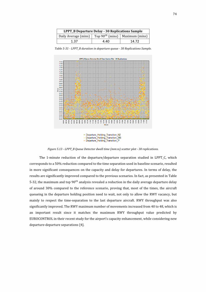
74

LPPT_B Departure Delay - 30 Replications Sample

Daily Average (mins) Top 90𝑡ℎ (mins) Maximum (mins)

1.37 4.40 14.72

Table 5-31 - LPPT_B duration in departure queue - 30 Replications Sample.

Figure 5.13 - LPPT_B Queue Detector dwell time (mm:ss) scatter plot - 30 replications.

The 1-minute reduction of the departure/departure separation studied in LPPT_C, which

corresponds to a 50% reduction compared to the time separation used in baseline scenario, resulted

in more significant consequences on the capacity and delay for departures. In terms of delay, the

results are significantly improved compared to the previous scenarios. In fact, as presented in Table

5-32, the maximum and top 90𝑡ℎ analysis revealed a reduction in the daily average departure delay

of around 30% compared to the reference scenario, proving that, most of the times, the aircraft

queueing in the departure holding position need to wait, not only to allow the RWY vacancy, but

mainly to respect the time-separation to the last departure aircraft. RWY throughput was also

significantly improved. The RWY maximum number of movements increased from 40 to 48, which is

an important result since it matches the maximum RWY throughput value predicted by

EUROCONTROL in their recent study for the airport’s capacity enhancement, while considering new

departure-departure separations [4].

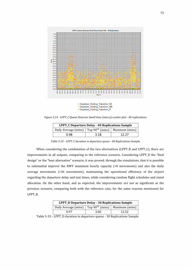
75

Figure 5.14 - LPPT_C Queue Detector dwell time (mm:ss) scatter plot - 40 replications.

LPPT_C Departure Delay - 40 Replications Sample

Daily Average (mins) Top 90𝑡ℎ (mins) Maximum (mins)

0.98 3.18 12.27

00:07:29

00:07:29

Table 5-32 - LPPT_C duration in departure queue - 40 Replications Sample.

When considering the combination of the two alternatives (LPPT_B and LPPT_C), there are

improvements in all outputs, comparing to the reference scenario. Considering LPPT_D the “final

design” or the “best alternative” scenario, it was proved, through the simulations, that it is possible

to substantial improve the RWY maximum hourly capacity (+8 movements) and also the daily

average movements (+36 movements), maintaining the operational efficiency of the airport

regarding the departure delay and taxi times, while considering random flight schedules and stand

allocation. On the other hand, and as expected, the improvements are not as significant as the

previous scenario, comparing both with the reference case, for the same reasons mentioned for

LPPT_B.

LPPT_D Departure Delay - 30 Replications Sample

Daily Average (mins) Top 90𝑡ℎ (mins) Maximum (mins)

0.97 3.00 12.52

Table 5-33 - LPPT_D duration in departure queue - 30 Replications Sample.

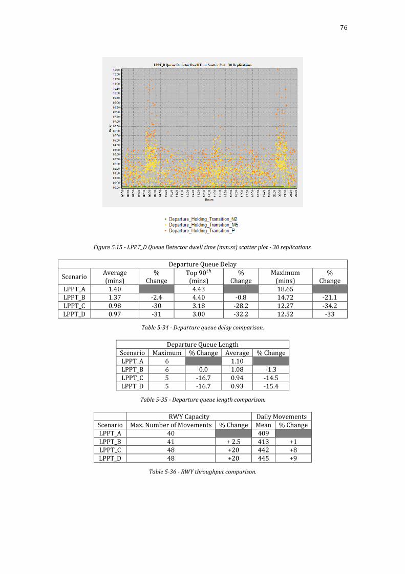
76

Figure 5.15 - LPPT_D Queue Detector dwell time (mm:ss) scatter plot - 30 replications.

Departure Queue Delay

Scenario Average (mins)

% Change

Top 90𝑡ℎ (mins)

% Change

Maximum (mins)

% Change

LPPT_A 1.40 4.43 18.65 LPPT_B 1.37 -2.4 4.40 -0.8 14.72 -21.1 LPPT_C 0.98 -30 3.18 -28.2 12.27 -34.2 LPPT_D 0.97 -31 3.00 -32.2 12.52 -33

Table 5-34 - Departure queue delay comparison.

Departure Queue Length Scenario Maximum % Change Average % Change LPPT_A 6 1.10 LPPT_B 6 0.0 1.08 -1.3 LPPT_C 5 -16.7 0.94 -14.5 LPPT_D 5 -16.7 0.93 -15.4

Table 5-35 - Departure queue length comparison.

RWY Capacity Daily Movements Scenario Max. Number of Movements % Change Mean % Change LPPT_A 40 409 LPPT_B 41 + 2.5 413 +1 LPPT_C 48 +20 442 +8 LPPT_D 48 +20 445 +9

Table 5-36 - RWY throughput comparison.

77

6 Conclusions and Further Research

Regarding EUROCONTROL’s “Humberto Delgado + Montijo” solution for the urgent Lisbon’s

airport capacity issues and since it is the local air navigation expert’s belief that, in order to increase

the airport’s capacity, it is imperative to reduce the waiting time for arrivals and departures by

reducing the runway occupancy times and implementing less restrictive departure air space

separations, this document focused on the maneuvering area and on the departure procedures.

Firstly, airport capacity concepts were studied. Since Lisbon’s airport is having capacity issues

mainly on the major traffic hours, Ultimate Capacity concept was found to be the most suitable for

these purposes. This way, by entering a continuous demand for both arrivals and departures flights,

it was possible to study the extreme hypothetic situation where there is always an aircraft waiting to

land or to take off. Since the focus was on the airport’s maneuvering area and on the departure

operations, the departure delay (on ground) was another major data analysis.

Secondly, the major capacity enhancement approaches were analyzed. Most of the literature

reviewed stated that the major approaches are restricted to two major groups, coinciding with the

approaches initially suggested by the local air navigations experts for Humberto Delgado:

minimization of aircraft separations and runway occupancy times. With the lack of available area for

construction around the airport, at first, a previous EUROCONTROL recommendation was studied:

study of a new RET to RWY 03. Then, with the separations between aircraft in mind and, with some

expertise advise, another solution was studied: reducing the departure-departure time separation

by half, as in ICAO’s regulations.

In order to study the alternatives, the different airport modelling approaches were reviewed.

This study helped to evidence the viability of using fast-time simulations in airport capacity analysis

with reliable results. A network model for the airport was created and, this way, it was possible to

visualize the aircraft movements after introducing the modifications in the airport, which helped in

the tradeoff analysis between capacity improvements and ground operations trustworthiness. The

software chosen was also suitable for this type of research. CAST was the right choice since it

provided a user-friendly interface and efficient tools which facilitated not only the airport models

creation but also the output analysis.

The technical approach followed was adequate . Based on the available data (airport charts

and ACE’s exercise) and with the adaptation of some inputs, the model was correctly structured and

configured. The traffic generation method and the random stand allocation resulted in typical airport

operations during low and high demand hours. In fact, the baseline scenario was properly calibrated

regarding the declared capacity of the airport the typical taxi times and the delay data.

78

After the baseline scenario calibration, the main objectives of the study were achieved. The

results obtained with the simulations were consistent and, after comparing the scenarios, it can be

concluded that the airport’s capacity could be increased with the introduction of the new runway exit

and, most important, with the introduction of less restrictive aircraft separation in the airport’s

terminal maneuvering area for departures in RWY 03. The introduction of the new exit resulted in a

statistical significant increase of 1 hourly movement during the traffic peaks and in an increase of 4

movements in the daily mean. Better results were obtained with the 1-minute reduction in the

departure time separations: an increase of 7 movements during the traffic peaks and 33 movements

increase of the daily traffic. As expected, the best results were obtained with the combination of the

other two alternatives: increase of 7 movements during the peak hours and 36 daily movements. In

the three alternative scenarios the mean results for the time spent by the aircraft in queue and the

queue length were reduced proving also the benefits in terms of ground movement bottlenecks.

In this document, as inherent to the process of modelling, some simplifications were done.

Despite this, the adaptations were only applied to the model providing that those would not affect it

directly in terms of respecting the real world regulations and deviating from typical operational

procedures of the airport. Nevertheless, there is room for further research:

In the future, inputting different ground dynamics per aircraft type and per replication may

result in interesting conclusions that could then be compared to the three aircraft categorization

used in this document. This could be done, for example, by means of distributions in the inputs,

or by entering more types of aircraft with different acceleration profiles and air/ground

behavior.

In this document, the airspace segments serve as entrance or exit to the model, with the

restrictions applied to airspace movements being the separation between aircraft, according to

their type, and to whether there are departure aircraft waiting in a queue or not. In the future, as

the runway capacity is directly affected by the airport terminal airspace, one development could

be the introduction of more complex airspace models. In addition, alongside one of the

alternatives of this study, there is also the need to study what would have to be the new airspace

configurations in order to achieve the requirements for less restrictive departure separations. In

order to do that, another airspace specific software, such as RAMS, could be used, since the core

focus of CAST is on the airport airside and terminal topics.

The method for the generation of traffic and the stand allocation rules were modified due mainly

to the need of assessing the capacity of the runway in as many scenarios as possible. Despite the

satisfactory results, testing the model with real flight schedules is something to consider in the

future.

79

Although the runway system capacity is usually recognized as the major airport capacity limiting

factor, other infrastructure elements should not be neglected a priori. In the particular case of

the taxiway system, despite some local constraints due to taxiway locations or configurations,

especially in the areas of taxiway intersections, the taxiway system it is most often designed to

provide capacity which exceeds the capacity of the runway system and should not be analyzed

as the factor limiting its capacity [12]. However, the development of the Lisbon’s airport taxiway

system is something to consider in the future and a similar study, with a similar fast-time

simulation software, could be used for that purpose.

80

References

[1] IATA, 19 September 2016. [Online]. Available: http://www.iata.org/about/Pages/history_3.aspx. [Acedido em 19 September 2016].

[2] Ministério das Comunicações, “Estudo da localização do novo aeroporto de Lisboa,” Imprensa Nacional, Lisboa, 1972.

[3] EUROCONTROL, 2016. [Online]. Available: https://ext.eurocontrol.int/airport_corner_public/LPPT. [Acedido em 19 September 2016].

[4] Dinheiro Vivo, “Montijo é a única “opção tecnicamente viável” para a Portela,” Dinheiro Vivo, Lisboa, 2016.

[5] Online Coordination System, 19 September 2016. [Online]. Available: https://www.online-coordination.com/Default.aspx?tabid=AvailTime. [Accessed 19 September 2016].

[6] R. Horonjeff e F. X. McKelvey, Planning and design of airports, New York: McGraw-Hill, 1983.

[7] LeighFisher et al, “Evaluating Airfield Capacity (Vol.79),” Transportation Research Board, Burlingame, CA, 2012.

[8] Airports Council International, “Guide to Airport performance measures,” Oliver Wyman, Inc., Quebec, 2012.

[9] ICAO, Airport Economics Manual, 2013.

[10] N. J. Ashford e P. H. Wright, Airport engineering, 2nd ed., New York: Wiley-Interscience, 1984.

[11] M. Janic, “Modelling the Capacity of Closely-Spaced Parallel Runways Using Innovative Approach Procedures,” Transportation Research Part C, Volume 16, Issue 6, pp. 704-730, 2008.

[12] R. De Neufville e A. R. Odoni, Airport systems, New York: McGraw-Hill, 2003.

[13] FAA, “Airport Capacity and Delay - Advisory Circular No 150/5060-S,” 1983.

[14] S. Hockaday e A. Kanafani, “Developments in Airport Capacity Analysis,” Transportation Research Vol. 8, pp. 171-180, 1974.

[15] F. Poldy, Airport Runway Capacity and Delay : Some Models for Planners and Managers, Canberra: Australian Government Publishing Service, 1982.

[16] K.-L. Tamas, “The Influence of Runway Occupancy Time and Wake Vortex Separation Requirements on Runway Throughput,” University of Florida, 2013.

[17] Hong Kong International Airport, “Hong Kong International Airport Master Plan 2030 - Technical Report,” [Online]. Available: http://hkia3way.blob.core.windows.net/pdf/en/TR_24May_Eng_Full.pdf. [Acedido em 14 December 2016].

[18] B. Mirkovic, “Airfield Modelling - State of the Art,” Faculty of Transport and Traffic Engineering, University of Belgrade, Belgrade, Serbia, 2015.

[19] A. Blumstein, “The Landing Capacity of a Runway,” Operations Research, pp. 752-763, 1959.

[20] EUROCONTROL, “RECAT-EU - European Wake Turbulence Categorisation and Separation Minima on Approach and Departure,” EUROCONTROL Headquarters, Brussels, 2015.

[21] EUROCONTROL, “Crosswind - Reduced Separations for Departure Operations (CREDOS),” [Online]. Available: http://www.eurocontrol.int/credos. [Acedido em 16 February 2017].

[22] ICAO, Air Traffic Management - Procedures for Air Navigation Services (Doc 4444) (Fifteen Edition ed.), ICAO, 2007.

[23] EUROCONTROL, 2016. [Online]. Available: http://www.eurocontrol.int/articles/wake-vortex. [Acedido em 20 September 2016].

[24] ICAO, “Air Traffic Services Planning Manual,” 2016. [Online]. Available: http://www2010.icao.int/EURNAT/Other%20Meetings%20Seminars%20and%20Workshops/Global%20ATFM%20Manual%20Coordination%20Team/1st%20Meeting%20at%20ATC%20Global%202012%20and%20EUROCONTROL%20CFMU/ICAO%20Doc%209426_cons_en.pdf. [Acedido em 20 September 2016].

[25] EUROCONTROL, “Wake turbulence aspects of Airbus A380-800 aircraft,” 2008. [Online]. Available: https://www.eurocontrol.int/sites/default/files/field_tabs/content/documents/nm/airports/airports-wake-vortex-aspects-letter-a380-aircraft1.pdf. [Acedido em 20 September 2016].

[26] M. Janic, “Toward Time-Based Separation Rules for Landing Aircraft,” Transportation research record, no. 2052, pp. 79-89.

81

[27] Eurocontrol, “Guidelines on Runway Capacity Enhancement,” European Air Traffic Management Programme, 2001.

[28] V. Kumar e L. Sherry, “Runway Occupancy Time Extraction and Analysis,” 2009.

[29] Federal Aviation Administration, “Aeronautical Information Manual,” 2012.

[30] C. Barbas, J. Vázquez e P. López, “Development of an Algorithm to model the landing operations, based on statistical analysis of actual data survey - ProESTOP,” Madrid, Spain, 2007.

[31] S. Pavlin, M. Zuzic e S. Pavicic, “Runway occupancy time as element of runway capacity,” Promet - Traffic& Transportation, vol. 18, no. 4, pp. 293-299, 2006.

[32] INECO, “Development of an Algorithm to model the landing operations, based on statistical analysis of actual data survey - ProESTOP,” Barcelona, 2007.

[33] R. R. Read e T. Yoshikawaf, “Operations analysis of locating high-speed runway exits,” Operations Research, 1962.

[34] M. Bazargan, K. Flemine e P. Subramanian, “A simulation study to investigate runway capacity using TAAM,” em Proceedings of the 2082 Winter Simulation Conference , Daytona Beach, FL, U.S., 2002.

[35] ICAO, “Annex 14 - Aerodromes - Volum I - Aerodrome Design and Operations,” em Convention on International Civil Aviation, 2013.

[36] ICAO, Aerodrome Design Manual - Part 2: Taxiways, Aprons and Holding Bays, 2005.

[37] H. D. Sherali, A. G. Hobeik, A. A. Trani e B. J. Kim, “An Integrated Simulation and Dynamic Programming Approach for Determining Optimal Runway Exit Locations,” Management Science, Vols. %1 de %2No. 7, Vol. 38, pp. 1049-1062, 1992.

[38] A. Odoni, J. Bowman, D. Delahaye, J. Deyst, E. Feron, R. Hansman, K. Khan, J. Kuchar, N. Pujet e R. Simpson, “Existing and Required Modeling Capabilities for Evaluating ATM Systems and Concepts,” Massachusetts Institute of Technology, Cambridge, U.S., 1997.

[39] A. Borshchev e A. Filippov, “From System Dynamics and Discrete Event to Practical Agent Based Modelling: Reasons, Techniques, Tools,” em The 22nd International Conference of the System Dynamics Society, Oxford, England, 2004.

[40] AnyLogic, “AnyLogic Features,” 20 September 2016. [Online]. Available: http://www.anylogic.com/features. [Accessed 20 September 2016].

[41] B. Burmeister, A. Haddadi e G. Matylis, “Application of multi-agent systems in traffic and transportation,” em IEE Proceedings - Software Engineering , Berlin, Germany, 1997.

[42] A. Borshchev e A. Filippov, “From System Dynamics and Discrete Event to Practical Agent Based Modelling: Reasons, Techniques, Tools,” St. Petersburg, Russia, 2004.

[43] R. Harris, “Models for runway capacity analysis,” Langley, Virginia, U.S., 1972.

[44] V. Tos̆ic e R. Horonjeff, “Effect of multiple path approach procedures on runway landing capacity,” Transportation research, 10(5), pp. 319-329, 1976.

[45] M. Janic, “Expansion of Airport Capacity: Case of London Heathrow Airport,” Transportation Research Record, pp. 7-14 , 2004.

[46] C. Divaris e V. Psaraki-Kalouptsidi, “Estimation of the Runway Capacity of the,” em Proceedings of the 12th Air Transport Research Society Conference, Athens, Greece, 2008.

[47] J. Barrer e P. Kuzminski, “Analyzing the Runway Capacity of Complex Airports,” em Proceedings of the 6th USA/Europe Air Traffic Management R&D Seminar, Baltimore, MD, U.S., 2005.

[48] J. Barrer, ““A New Method for Modeling Complex Runway Systems,” em Proceedings of the 7th USA/Europe Air Traffic Management R&D Seminar, Barcelona, Spain, 2007.

[49] P. T. Fishburn e M. Stouppe, “ Simulation: a powerful planning tool.,” em Airpon Modeling and Simulafion: Conference Proceedings, August 17-20, Key Bridge Marriot Hotel, Arlington, Virginia, 1997.

[50] P. D. E. e E. A. Jerrard, “Monte-Carlo comes to Rome: a note on the estimation of unconstrained runway capacity at Rome Fiumucino International Airport,” Journal ofAir Transport Management, vol. 5, pp. 185-192, 1999.

[51] D. E. Pitfield, A. S. Brooke e E. A. Jerrard, “Monte-Carlo simulation of potentially conflicting ground movements at a new international airport,” Journal ofAir Transport Management , vol. 4, pp. 3-9, 1998.

[52] D. Irvine, L. C.S. Budd e D. E. Pitfield, “A Monte-Carlo approach to estimating the effects of selected airport capacity options in London,” Journal of Air Transport Management, vol. 42, pp. 1-9, 2015.

[53] W. Chao, Z. Xinyue e X. Xiaohao, “Simulation Study on Airfield System Capacity Analysis Using SIMMOD,” Civil Aviation University of China, Tianjin 300300, China , 2008.

[54] R. Florio Moser, “Simulação e análises de configurações aeroportuárias utilizando Visual SIMMOD:aplicação ao aeroporto internacional de São Paulo/Guarulhos,” São Paulo, Brasil, 2007.

82

[55] B. Bubalo e J. R. Daduna, “Airport capacity and demand calculations by simulation - the case of Berlin-Brandenburg,” Berlin School of Economics and Law, Germany, 2012.

[56] R. Araújo Almeida, “Análise de alternativas para aumento de capacidade operacional do Aeroporto Internacional de São Paulo/Guarulhos,” São Paulo, Brasil, 2012.

[57] M. Bazargan, K. Flemine e P. Subramanian, “A simulation study to investigate runway capacity using TAAM,” Embry Riddle Aeronautical University, USA, 2002.

[58] S. Theiss, “Support of the Determination of the Declared Capacity by the Use of Airside Simulation for Runway Capacity Analysis,” Aerlines Magazine, Vols. %1 de %2e-zine edition 41, nº Aviation Simulation, 2007.

[59] E. P. Gilbo, “Airport capacity: representation, estimation, optimization,” IEEE Transactions on Control Systems Technologies, Vols. %1 de %21, No3, pp. 144-154, 1993.

[60] P. Böck e M. Hornung, “Airport capacity representation based on airside simulations,” Munich, Germany , 2012.

[61] M. M. Breunig, H.-P. Kriegel, R. T. Ng e J. Sander, “LOF: Identifying Density-Based Local Outliers,” Dalles, TX, 2000.

[62] EUROCONTROL, “,” 29 June 2011 . [Online]. Available: https://www.eurocontrol.int/eec/public/standard_page/WP_Fast_Time_Simulation_Tools.html. [Acedido em 26 October 2016].

[63] X. Zou e P. Cheng, “A Simulation Model for Airport Runway Capacity Estimation,” Qingdao, China, 2014.

[64] Y. Peng, G. Wei e S. Jun-Qing, “Capacity Analysis for Parallel Runway through Agent-Based Simulation,” Ming Cao, Tianjin 300300, China, 2013.

[65] CAST, “CAST Simulation,” 2016. [Online]. Available: http://www.airport-consultants.com/cast-simulation. [Acedido em 20 September 2016].

[66] ANA Aeroportos de Lisboa, 22 March 2016. [Online]. Available: http://www.ana.pt/pt-PT/Aeroportos/Lisboa/Lisboa/OAeroporto/ConhecaoAeroporto/Paginas/Conheca-o-Aeroporto.aspx.

[67] M. v. d. Hoofd, “Airliners,” 26 April 2008. [Online]. Available: http://www.airliners.net/photo/-/-/1681723/L?qsp=eJwtjbEOwjAQQ38F3cwEEkM3%2BgMw8ANHYtGI0ER3p7ZR1X8nKWy2n2Wv5NJoWOxRMqgjBYsb6EiZhT9K3UpvlDmJr5pi0GcaD2mCTAFzrWkS60tFng1X55AN/p/fxEMagrp98dUeTk1C7j93vlTrg%2BbI%2BwqMQ6Rt%2BwK8iDL%2B. [Acedido em 14 December 2016].

[68] NAV/EUROCONTROL, “Lisbon Capacity Enhancement Exercise 2010-2011,” 2011.

[69] Lusa, 18 March 2016. [Online]. Available: http://economico.sapo.pt/noticias/ana-quer-decisao-sobre-aeroporto-em-lisboa-este-ano_245270.html.

[70] J. G. P. D. A. Coelho, “Análise de Novos Procedimentos Operacionais de Gestão de Chegadas em Espaço Aéreo Terminal,” IST, Lisboa, 2016.

[71] NAV Portugal, “Lisbon Capacity Enhancement Exercise 2010-2011,” 2011.

[72] EUROCONTROL/CODA, “CODA Publications,” [Online]. Available: http://www.eurocontrol.int/articles/coda-publications. [Acedido em 16 January 2017].

[73] EUROCONTROL/CODA, “All-Causes Delay and Cancellations to Air Transport in Europe – Annual 2015,” CODA, 2015.

[74] EUROCONTROL, European Airspace Concept Handbook for PBN Implementation, 2013.

[75] Airport Research Center, “CAST Aircraft Tutorial,” 2014.

[76] N. M. Razali e Y. B. Wah, “Power comparison of Shapiro-Wilk, Kolmogorov-Smirnov, Lilliefors and Anderson-Darling tests,” Journal of Statistical Modelling and Analytics, vol. Vol.2 No.1 , pp. 21-33, 2011.

[77] J. Royston, “An extension of Shapiro and Wilk's W Tests for Normality to Large Samples,” Applied Statistics, vol. 31, pp. 115-124, 1982.

[78] “Real Statistic Using Excel,” 2017. [Online]. Available: http://www.real-statistics.com/tests-normality-and-symmetry/statistical-tests-normality-symmetry/shapiro-wilk-expanded-test/. [Acedido em 06 March 2017].

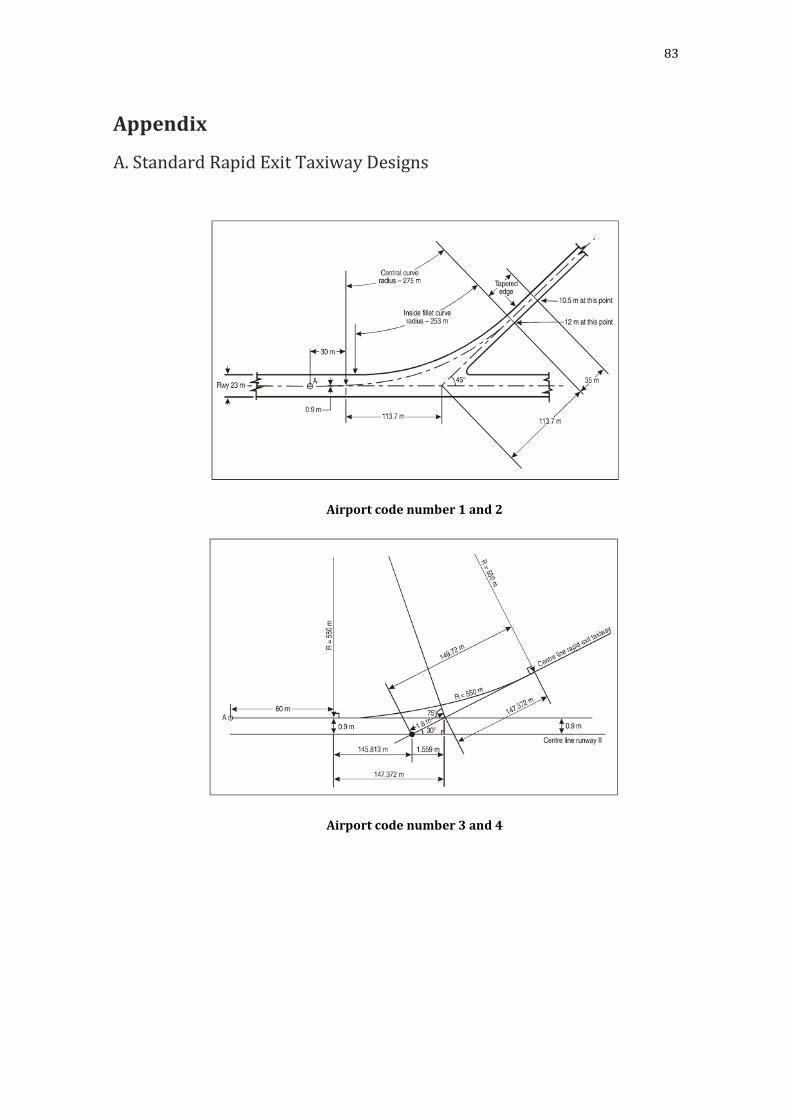
83

Appendix

A. Standard Rapid Exit Taxiway Designs

Airport code number 1 and 2

Airport code number 3 and 4

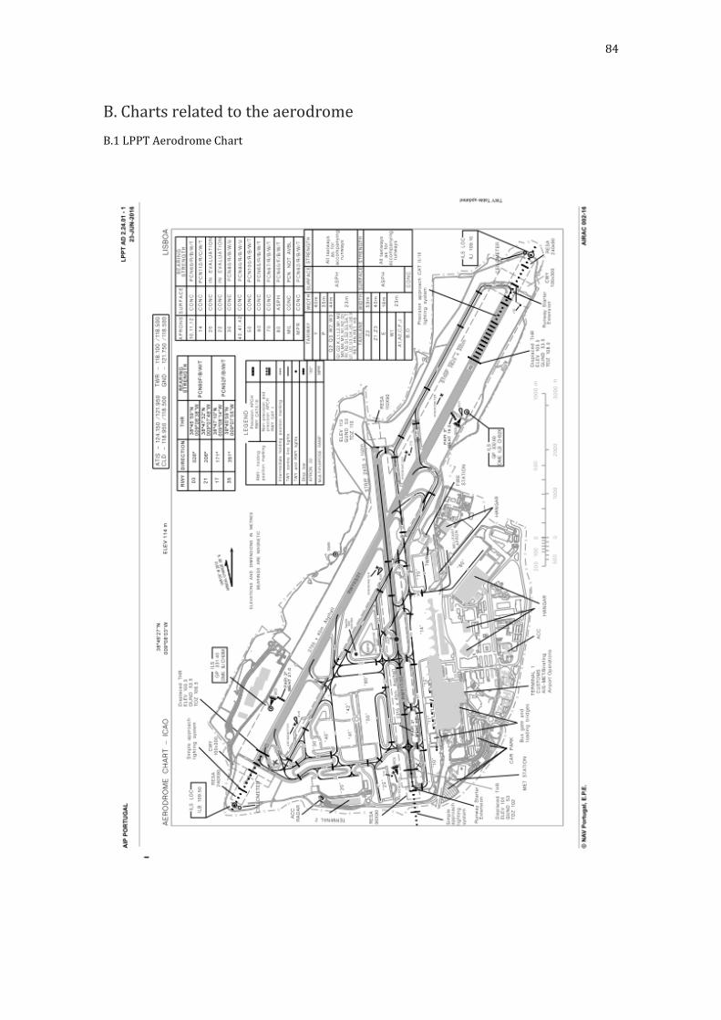
84

B. Charts related to the aerodrome

B.1 LPPT Aerodrome Chart

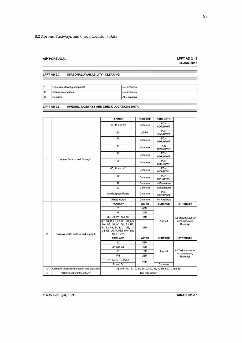
85

B.2 Aprons, Taxiways and Check Locations Data

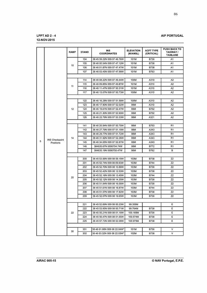
86

87

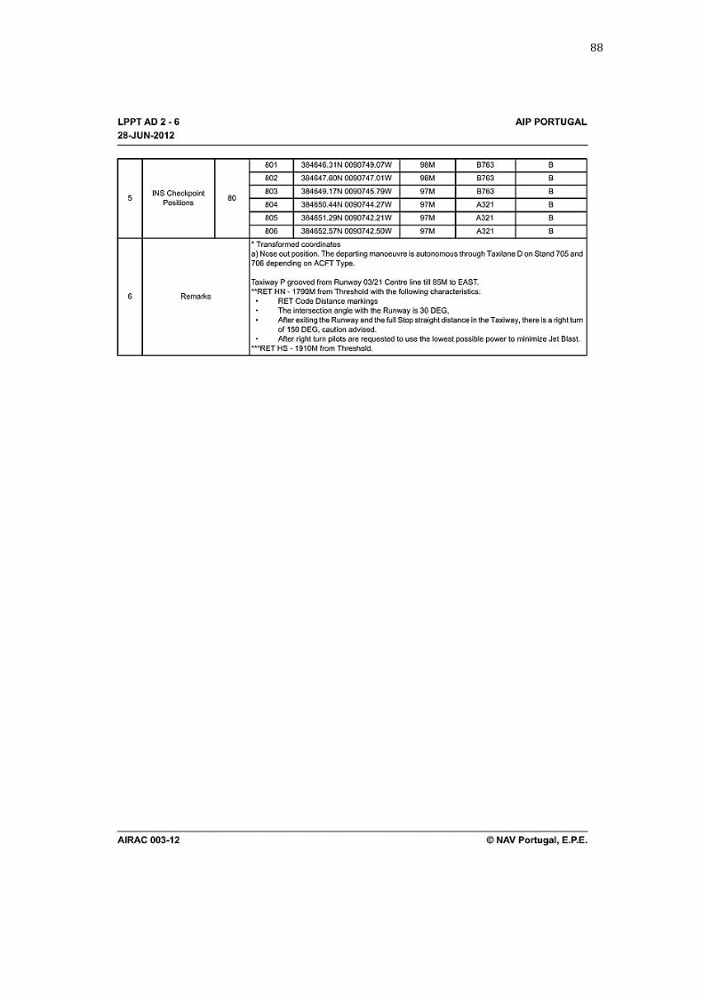
88

89

B.3 Ground Movement Chart Arr/Dep RWY 03

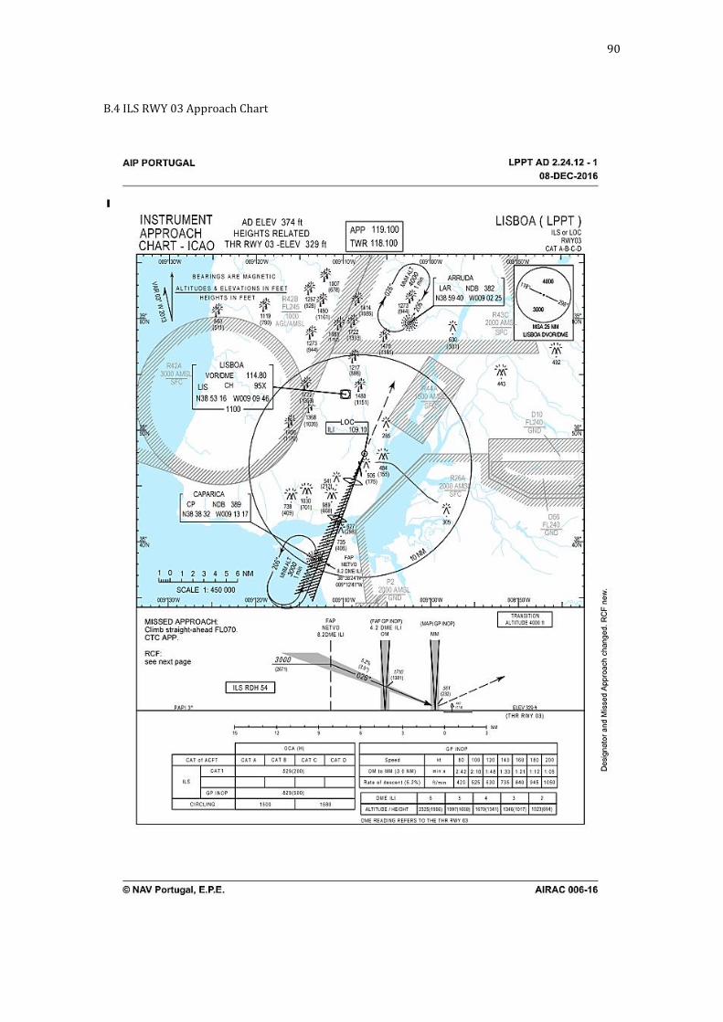
90

B.4 ILS RWY 03 Approach Chart

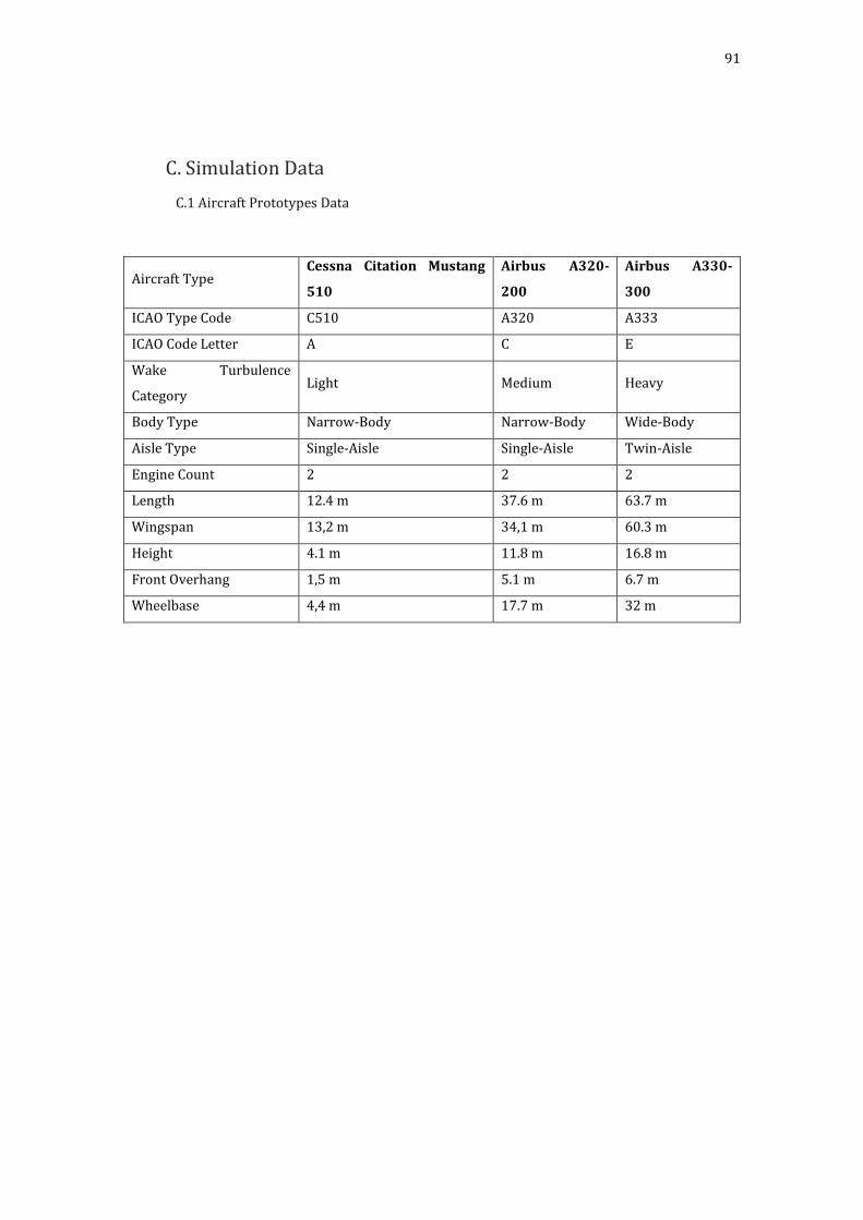
91

C. Simulation Data

C.1 Aircraft Prototypes Data

Aircraft Type Cessna Citation Mustang

510

Airbus A320-

200

Airbus A330-

300

ICAO Type Code C510 A320 A333

ICAO Code Letter A C E

Wake Turbulence

Category Light Medium Heavy

Body Type Narrow-Body Narrow-Body Wide-Body

Aisle Type Single-Aisle Single-Aisle Twin-Aisle

Engine Count 2 2 2

Length 12.4 m 37.6 m 63.7 m

Wingspan 13,2 m 34,1 m 60.3 m

Height 4.1 m 11.8 m 16.8 m

Front Overhang 1,5 m 5.1 m 6.7 m

Wheelbase 4,4 m 17.7 m 32 m

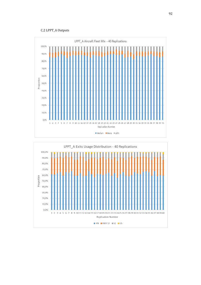
92

C.2 LPPT_A Outputs

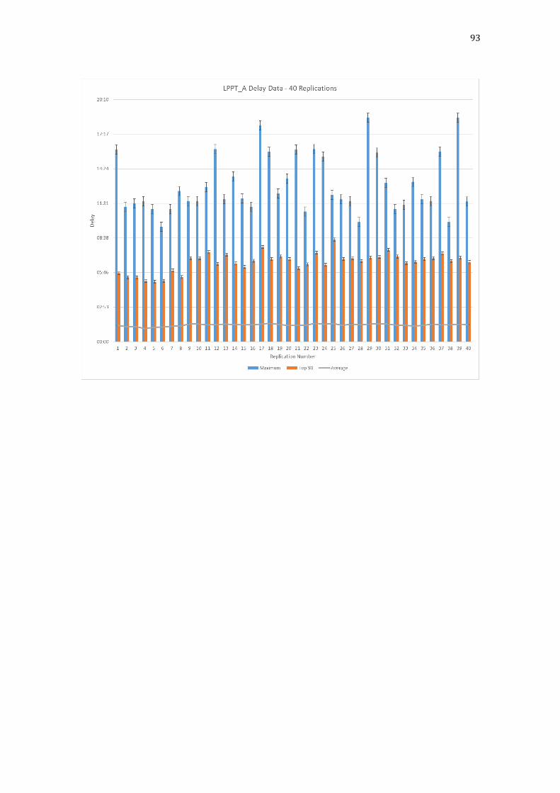
93

94

C.3 LPPT_B Outputs

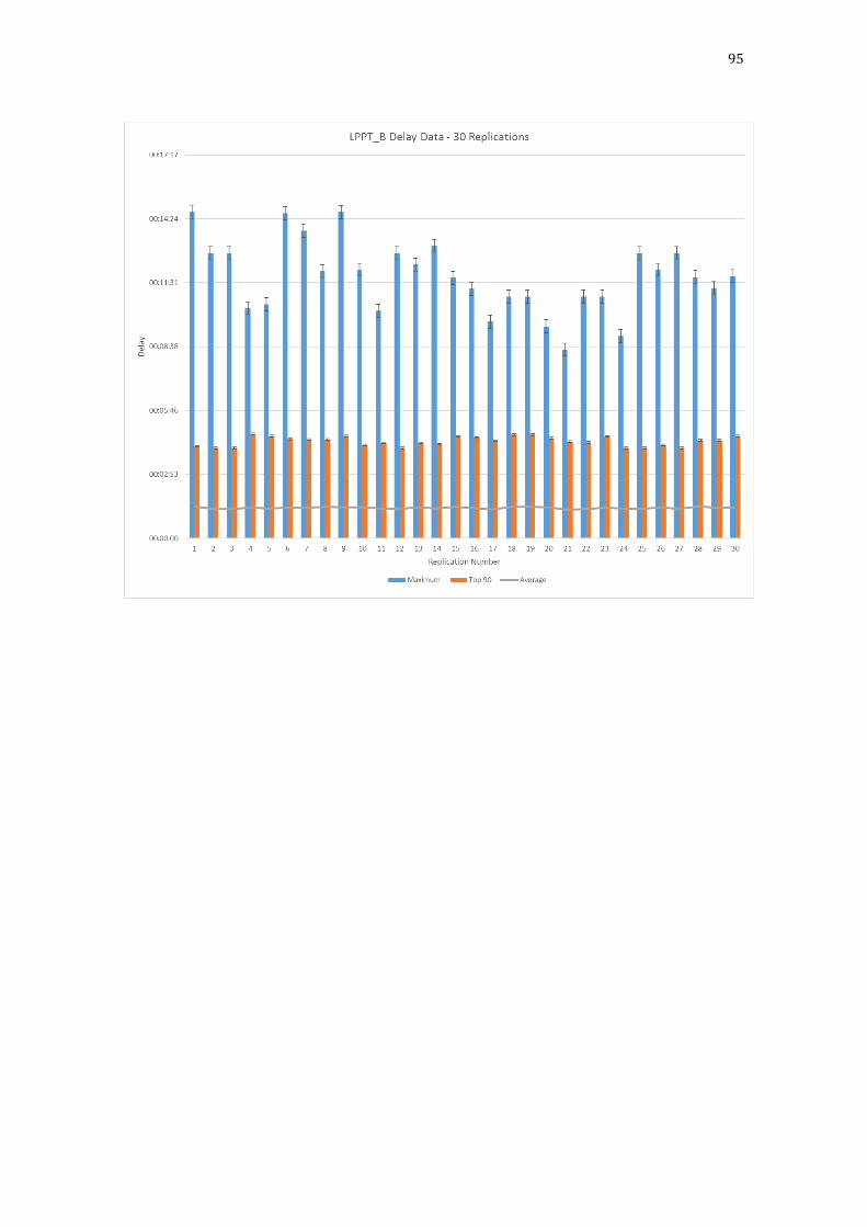
95

96

C.4 LPPT_C Outputs

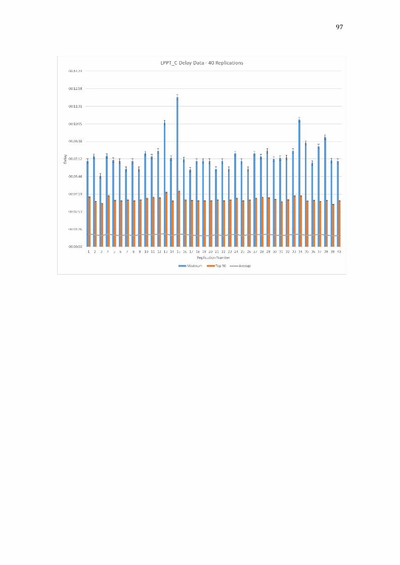
97

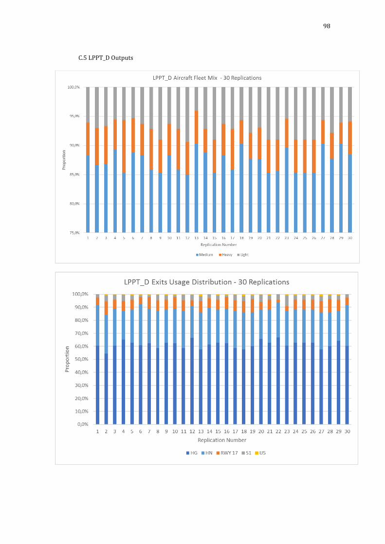
98

C.5 LPPT_D Outputs

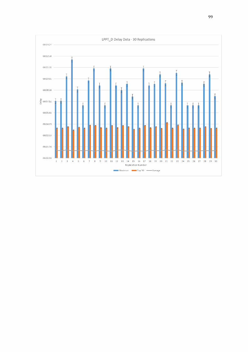
99