ACCELERATION OF CONVERGENCE IN DONTCHEV'S ITERATIVE METHOD FOR SOLVING VARIATIONAL INCLUSIONS

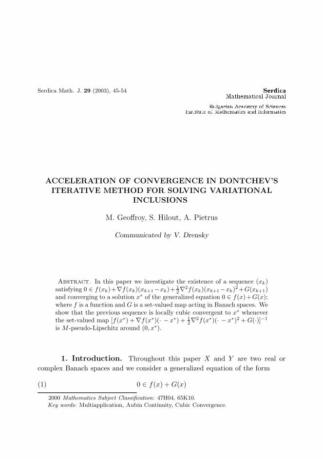
Serdica Math. J. 29 (2003), 45-54

ACCELERATION OF CONVERGENCE IN DONTCHEV’S

ITERATIVE METHOD FOR SOLVING VARIATIONAL

INCLUSIONS

M. Geoffroy, S. Hilout, A. Pietrus

Communicated by V. Drensky

Abstract. In this paper we investigate the existence of a sequence (xk)satisfying 0 ∈ f(xk)+∇f(xk)(xk+1−xk)+ 1

2∇2f(xk)(xk+1−xk)2+G(xk+1)

and converging to a solution x∗ of the generalized equation 0 ∈ f(x)+G(x);where f is a function and G is a set-valued map acting in Banach spaces. Weshow that the previous sequence is locally cubic convergent to x∗ wheneverthe set-valued map [f(x∗) +∇f(x∗)(· − x∗) + 1

2∇2f(x∗)(· − x∗)2 +G(·)]−1

is M -pseudo-Lipschitz around (0, x∗).

1. Introduction. Throughout this paper X and Y are two real or

complex Banach spaces and we consider a generalized equation of the form

0 ∈ f(x) +G(x)(1)

2000 Mathematics Subject Classification: 47H04, 65K10.Key words: Multiapplication, Aubin Continuity, Cubic Convergence.

46 M. Geoffroy, S. Hilout, A. Pietrus

where f is a function from X into Y an G is a set-valued map from X to the

subsets of Y .

When G = ∂ψC is the subdifferential of the function

ψC(x) =

{

0 if x ∈ C

+∞ otherwise,

(1) has been studied by Robinson [10]. The key of his idea is to associate to (1)

a linearized equation. His study concerns especially the stability of solutions of

some minimization problems.

When ∇f is locally Lipschitz Dontchev [4] associates to (1) a Newton-

type method based on a partial linearization which provides a local quadratic

convergence. Following his work, Pietrus [9] obtains a Newton-type sequence

which converges whenever ∇f satisfies a Holder-type condition.

In this paper we associate to (1) the relation

0 ∈ f(xk) + ∇f(xk)(xk+1 − xk) +1

2∇2f(xk)(xk+1 − xk)

2 +G(xk+1),(2)

where ∇f(x) and ∇2f(x) denote respectivly the first and the second Frechet

derivative of f at x. One can note that if xk −→ x∗, then x∗ is a solution of (1).

Let us mention that relation (2) derives from a second-degree Taylor polynomial

expansion of f at xk and that such an approximation is an extension of Dontchev’s

original work [3].

The paper is organized as follows: in section 2 we recall a few preliminary

results and make some fundamental assumptions on f . Then, in section 3 we

prove the existence of a sequence (xk) satisfying (2) and we show that it is locally

cubic convergent.

2. Preliminaries and fundamental assumptions.

Definition 2.1. A set-valued map Γ : X −→ Y is said to be M -pseudo-

lipschitz around (x0, y0) ∈ graph Γ := {(x, y) ∈ X × Y | y ∈ Γ(x)} if there exist

neighbourhoods V of x0 and U of y0 such that

supy∈Γ(x1)∩U

dist(y,Γ(x2)) ≤M ‖ x1 − x2 ‖,∀x1, x2 ∈ V.(3)

Acceleration of convergence in Dontchev’s iterative method 47

When a multiapplication Γ is M -pseudo-Lipschitz, the constant M is

called the modulus of Aubin continuity.

The Aubin continuity of Γ is equivalent to the openess with linear rate

of Γ−1 (the covering property) and to the metric regularity of Γ−1 (a basic well-

posedness property in optimization).

Finally, when f is a function which is strictly differentiable at some x0,

then the Aubin continuity of f−1 around (f(x0), x0) is equivalent to the surjec-

tivity of ∇f(x0). For more details, the reader can refer to [1, 2, 8, 11, 12].

Let A and C be two subsets of X, we recall that the excess e from the set

A to the set C is given by e(C,A) = supx∈C

dist(x,A).

Then, we have an equivalent definition ofM -pseudo-Lipschitzness in terms

of excess by replacing (3) by

e(Γ(x1) ∩ U,Γ(x2)) ≤M ‖ x1 − x2 ‖,∀x1, x2 ∈ V,(4)

in the previous definition. In [6] the above property is called Aubin property and

in [5] it has been used to study the problem of the inverse for set-valued maps.

In the sequel, we will need the following fixed point statement which has been

proved in [5].

Lemma 2.1. Let (X, ρ) be a complete metric space, let φ a map from X

into the closed subsets of X, let η0 ∈ X and let r and λ be such that 0 ≤ λ < 1

and

a) dist (η0, φ(η0)) ≤ r(1 − λ),

b) e(φ(x1) ∩Br(η0), φ(x2)) ≤ λ ρ(x1, x2) ∀x1, x2 ∈ Br(η0),

then φ has a fixed point in Br(η0). That is, there exists x ∈ Br(η0) such that

x ∈ φ(x). If φ is single-valued, then x is the unique fixed point of φ in Br(η0).

The previous lemma is a generalization of a fixed-point theorem in [7],

where in (b) the excess e is replaced by the Haussdorff distance.

We suppose that x∗ ∈ X is a solution of equation (1). Before studying our

problem, we make the following assumptions:

(H0) G has closed graph;

(H1) f is Frechet differentiable on some neighborhood V of x∗;


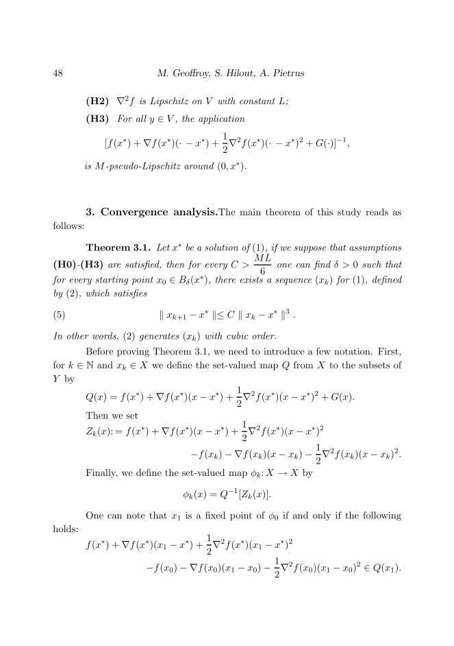
(H2) ∇2f is Lipschitz on V with constant L;

(H3) For all y ∈ V , the application

[f(x∗) + ∇f(x∗)(· − x∗) +1

2∇2f(x∗)(· − x∗)2 +G(·)]−1,

is M -pseudo-Lipschitz around (0, x∗).

3. Convergence analysis.The main theorem of this study reads as

follows:

Theorem 3.1. Let x∗ be a solution of (1), if we suppose that assumptions

(H0)-(H3) are satisfied, then for every C >ML

6one can find δ > 0 such that

for every starting point x0 ∈ Bδ(x∗), there exists a sequence (xk) for (1), defined

by (2), which satisfies

‖ xk+1 − x∗ ‖≤ C ‖ xk − x∗ ‖3 .(5)

In other words, (2) generates (xk) with cubic order.

Before proving Theorem 3.1, we need to introduce a few notation. First,

for k ∈ N and xk ∈ X we define the set-valued map Q from X to the subsets of

Y by

Q(x) = f(x∗) + ∇f(x∗)(x− x∗) +1

2∇2f(x∗)(x− x∗)2 +G(x).

Then we set

Zk(x):= f(x∗) + ∇f(x∗)(x− x∗) +1

2∇2f(x∗)(x− x∗)2

−f(xk) −∇f(xk)(x− xk) −1

2∇2f(xk)(x− xk)

2.

Finally, we define the set-valued map φk:X → X by

φk(x) = Q−1[Zk(x)].

One can note that x1 is a fixed point of φ0 if and only if the following

holds:

f(x∗) + ∇f(x∗)(x1 − x∗) +1

2∇2f(x∗)(x1 − x∗)2

−f(x0) −∇f(x0)(x1 − x0) −1

2∇2f(x0)(x1 − x0)

2 ∈ Q(x1).


Thus, it is easy to see that the previous assertion is equivalent to

0 ∈ f(x0) + ∇f(x0)(x1 − x0) +1

2∇2f(x0)(x1 − x0)

2 +G(x1).(6)

Once xk is computed, we show that the function φk has a fixed point xk+1 in X.

This process allows us to prove the existence of a sequence (xk) satisfying (2).

Now, we state a result which is the starting point of our algorithm. It

will be very usefull to prove Theorem 3.1 and reads as follows:

Proposition 3.1. Under the hypotheses of Theorem 3.1, there exists

δ > 0 such that for all x0 ∈ Bδ(x∗) (x0 6= x∗), the map φ0 has a fixed point x1 in

Bδ(x∗) satisfying ‖x1 − x∗‖ ≤ C‖x0 − x∗‖3.

P r o o f. By hypothesis (H3) there exist positive numbers a and b such

that

e(Q−1(y′) ∩Ba(x∗), Q−1(y′′)) ≤M ‖ y′ − y′′ ‖, ∀y′, y′′ ∈ Bb(0).(7)

Fix δ > 0 such that

δ < min

{

a,

(

2b

3L

)1

3

,1√C

}

.(8)

To prove Proposition 3.1 we intend to show that both assertions (a) and

(b) of Lemma 2.1 hold; where η0: = x∗, φ is the function φ0 defined at the very

begining of this section and where r and λ are numbers to be set.

According to the definition of the excess e, we have

dist (x∗, φ0(x∗)) ≤ e

(

Q−1(0) ∩Bδ(x∗), φ0(x

∗)

)

.(9)

Moreover, for all x0 ∈ Bδ(x∗) such that x0 6= x∗ we have

‖Z0(x∗)‖ = ‖f(x∗)− f(x0)−∇f(x0)(x

∗ − x0)−1

2∇2f(x0)(x

∗ − x0)2‖, so

‖Z0(x∗)‖ ≤ L

6‖x∗ − x0‖3.


Then (8) yields, ‖Z0(x∗)‖ < b. Hence from (7) one has

e

(

Q−1(0)∩Bδ(x∗), φ0(x

∗)

)

= e

(

Q−1(0)∩Bδ(x∗), Q−1[Z0(x

∗)]

)

≤ ML

6‖x∗−x0‖3.

By (9), we get

dist (x∗, φ0(x∗)) ≤ ML

6‖x∗ − x0‖3.(10)

Since C >ML

6there exists λ ∈ ]0, 1[ such that C(1 − λ) ≥ ML

6. Hence,

dist (x∗, φ0(x∗)) ≤ C(1 − λ)‖x∗ − x0‖3.(11)

By setting η0 := x∗ and r := r0 = C‖x∗ − x0‖3 we can deduce from the

last inequalities that assertion (a) in Lemma 2.1 is satisfied.

Now, we show that condition (b) of lemma 2.1 is satisfied. Since1√C

≥ δ

and ‖x∗ − x0‖ ≤ δ, we have r0 ≤ δ ≤ a.

Moreover for x ∈ Bδ(x∗),

‖Z0(x)‖ ≤ ‖f(x∗) − f(x) −∇f(x∗)(x− x∗) − 1

2∇2f(x∗)(x− x∗)2‖

+ ‖f(x) − f(x0) −∇f(x0)(x− x0) −1

2∇2f(x0)(x− x0)

2‖

≤ L

6‖x− x∗‖3 +

L

6‖x− x0‖3

≤ 3L

2δ3.

Then by (8) we deduce that for all x ∈ Bδ(x∗), Z0(x) ∈ Bb(0). Then it

follows that for all x′, x′′ ∈ Br0(x∗), we have

e(φ0(x′) ∩ Br0

(x∗), φ0(x′′)) ≤ e(φ0(x

′) ∩ Bδ(x∗), φ0(x

′′)), which yields by

(7):

e(φ0(x′) ∩Br0

(x∗), φ0(x′′)) ≤M‖Z0(x

′) − Z0(x′′)‖

≤M‖∇f(x∗)(x′ − x′′) −∇f(x0)(x′ − x′′)


+1

2∇2f(x∗)(x′ − x∗)2 − 1

2∇2f(x∗)(x′′ − x∗)2

+1

2∇2f(x0)(x

′′ − x0)2 − 1

2∇2f(x0)(x

′ − x0)2‖

≤M‖∇f(x∗)(x′ − x′′) −∇f(x0)(x′ − x′′)

+1

2∇2f(x∗)(x′ − x′′ + x′′ − x∗)2 − 1

2∇2f(x∗)(x′′ − x∗)2

+1

2∇2f(x0)(x

′′ − x0)2 − 1

2∇2f(x0)(x

′ − x′′ + x′′ − x0)2‖.

Assumption (H2) ensures the existence of L1 > 0 such that ‖∇2f‖ ≤ L1

on Bδ(x∗). Then an easy computation yields:

e(φ0(x′) ∩Br0

(x∗), φ0(x′′)) ≤ 5ML1δ‖x′ − x′′‖.(12)

Without loss of generality we may assume that δ <λ

5ML1thus condition

(b) of Lemma 2.1 is satisfied. Since both conditions of Lemma 2.1 are fulfilled,

we can deduce the existence of a fixed point x1 ∈ Br0(x∗) for the map φ0. Then

the proof of Proposition 3.1 is complete. �

Now that we proved Proposition 3.1, the proof of Theorem 3.1 is straight-

forward as it is shown below.

P r o o f o f Th e o r em 3.1. Proceeding by induction, keeping η0 = x∗

and setting rk = C‖xk − x∗‖3, the application of proposition 3.1 to the map φk

gives the existence of a fixed point xk+1 for φk, which is an element of Brk(x∗).

This last fact implies that :

‖ xk+1 − x∗ ‖≤ C ‖ xk − x∗ ‖3 .(13)

In others words, (2) generates a sequence (xk) with cubic order and the proof of

theorem 3.1 is complete. �

Corollary 3.1. Let x∗ be an isolated solution of (1), if assumptions

(H0)-(H3) are satisfied, then for every C >ML

6one can find δ > 0 such that

any sequence (xk) generated by (2) with xk ∈ Bδ(x∗) satisfies (5).


P r o o f. As we recalled it in the proof of Proposition 3.1, there exists

L1 > 0 such that ‖∇2f(x)‖ ≤ L1. Then, we fix δ satisfying both relation (8) and

the following:

δ < min

{

1

3ML1,6C −ML

18CML1

}

.(14)

Without loss of generality we may assume that the solution of (1) is unique

in B4δ(x∗). Let (xk) be a sequence generated by (2) with xk ∈ Bδ(x

∗), then x∗ is

the only point in B4δ(x∗) satisfying (1), i.e., x∗ = Q−1(0) ∩ B4δ(x

∗). Moreover,

for all k ∈ N, by Theorem 3.1 we have:

xk+1 ∈ Q−1[Zk(xk+1)].

Hence,

‖xk+1 − x∗‖ = dist (xk+1, Q−1(0)) then,

‖xk+1 − x∗‖ ≤ e

(

Q−1[Zk(xk+1)] ∩Bδ(x∗), Q−1(0)

)

,

‖xk+1 − x∗‖ ≤M‖Zk(xk+1)‖,

‖xk+1 − x∗‖ ≤M‖f(x∗) + ∇f(x∗)(xk+1 − x∗) +1

2∇2f(x∗)(xk+1 − x∗)2

−f(xk) −∇f(xk)(xk+1 − xk) −1

2∇2f(xk)(xk+1 − xk)

2‖.

Then, an easy computation shows that

‖xk+1 − x∗‖ ≤M

(

L

6‖x∗ − xk‖3 + 3L1δ‖xk+1 − x∗‖

)

.

Thus,

‖xk+1 − x∗‖ ≤ ML

6(1 − 3ML1δ)‖xk − x∗‖3.

Thanks to (14), we have C >ML

6(1 − 3ML1δ)so ‖xk+1−x∗‖ ≤ C ‖xk−x∗‖3

and then the proof is complete. �

Acknowledgement. The authors thank the referee for his valuable re-

marks and comments on this work.


REF ERENC ES

[1] J. P. Aubin. Lipschitz behavior of solutions to convex minimization prob-

lems. Math. Oper. Res. 9 (1984) 87–111.

[2] J. P Aubin, H. Frankowska. Set-valued Analysis. Birkhauser, Boston,

1990.

[3] A. L. Dontchev. Local analysis of a Newton-type method based on par-

tial linearization. In: The mathematics of numerical analysis (Eds Renegar,

James et al.) 1995 AMS-SIAM summer seminar in applied mathematics,

Providence, RI: AMS. Lect. Appl. Math. vol. 32 (1996), 295–306.

[4] A. L. Dontchev. Local convergence of the Newton method for generalized

equation, C. R. Acad. Sci. Paris Ser. I Math. 322, Serie I, (1996), 327–331.

[5] A. L. Dontchev, W. W. Hager. An inverse function theorem for set-

valued maps. Proc. Amer. Math. Soc. 121 (1994), 481–489.

[6] A. L. Dontchev, R. T. Rockafellar. Characterizations of strong regu-

larity for variational inequalities over polyhedral convex sets. SIAM J. Op-

tim. 6, 4 (1996), 1087–1105.

[7] A. D. Ioffe, V. M. Tikhomirov. Theory of Extremal Problems. North

Holland, Amsterdam, 1979.

[8] B. S. Mordukhovich. Complete characterization of openess metric regu-

larity and Lipschitzian properties of multifunctions. Trans. Amer. Math. Soc

340 (1993), 1–36.

[9] A. Pietrus. Generalized equation under mild differentiability conditions.

Rev. R. Acad. Cienc. Exactas Fis. Nat. (Esp.) 94, (1) (2000), 15–18.

[10] S. M. Robinson. Strong regular generalized equations. Math. of Oper. Res.

5 (1980), 43–62.

[11] R. T. Rockafellar. Lipschitzian properties of multifunctions. Nonlinear

Anal. 9 (1984), 867–885.

[12] R. T. Rockafellar, R. Wets. Variational Analysis. A Series of compre-

hensive studies in mathematics, Springer, vol. 317, 1998.


M. Geoffroy

A. Pietrus

Laboratoire Analyse, Optimisation, Controle

Universite des Antilles et de la Guyane

Departement de Mathematiques

et Informatique

Campus de Fouillole

F-97159 Pointe-a-Pitre

France

e-mail: [email protected]

e-mail: [email protected]

S. Hilout

Departement de Mathematiques

Appliquees et Informatique

Faculte des Sciences et Techniques

B.P. 523, Beni-Mellal

Maroc

Received August 13, 2002

Revised January 28, 2003

ACCELERATION OF CONVERGENCE IN DONTCHEV'S ITERATIVE METHOD FOR SOLVING VARIATIONAL INCLUSIONS

Documents

Transcript of ACCELERATION OF CONVERGENCE IN DONTCHEV'S ITERATIVE METHOD FOR SOLVING VARIATIONAL INCLUSIONS