ABCAnalytical and semi-analytical analysis of an artificial satellite’s rotational motion

ANALYTICAL AND SEMI-ANALYTICAL ANALYSIS OF ANARTIFICIAL SATELLITE’S ROTATIONAL MOTION

M. CECILIA ZANARDI and R. VILHENA DE MORAESGrupo de Dinamica Orbital e Planetologia, Department of Mathematics, UNESP - Campus de

Guaratingueta, Caixa Postal 205, 12500-000, Guaratinguet´a, SP, Brazil

(Received: 16 July 1997; accepted: 16 February 2000)

Abstract. The rotational motion of an artificial satellite is studied by considering torques producedby gravity gradient and direct solar radiation pressure. A satellite of circular cylinder shape is con-sidered here, and Andoyers variables are used to describe the rotational motion. Expressions fordirect solar radiation torque are derived. When the earth’s shadow is not considered, an analyticalsolution is obtained using Lagrange’s method of variation of parameters. A semi-analytical procedureis proposed to predict the satellite’s attitude under the influence of the earth’s shadow. The analyticalsolution shows that angular variables are linear and periodic functions of time while their conjugatessuffer only periodic variations. When compared, numerical and analytical solutions have a goodagreement during the time range considered.

Key words: rotational motion, solar radiation torque, Andoyer variables

1. Introduction

The main objective of this paper is to analyze the influence of external torques onthe rotational motion of an earth’s artificial satellite. Direct solar radiation pressureand gravity gradient were chosen as the external torques. Long period and seculareffects are emphasized.

Here Andoyer’s canonical variables (Kinoshita, 1972)(L1, L2, L3) and(l1, l2, l3), shown in Figure 1, are used to describe the motion of a body around itscenter of mass. Andoyer’s metric variablesLi, i = 1,2,3 are defined as follows:L2 is the modulus of the total angular momentum,L1 andL3 are respectively theprojection ofL2 on thez-axis’ principal axis system of inertia and on the inertialZ-axis. The Andoyer’s angular variablesli, i = 1,2,3, are related to the orientationof the body frame respectively to the inertial frame. The inertial system consideredis the equatorial system of the earth.

An analytical solution is derived assuming a circular cylindric type satellite.For some missions the order of the magnitude of the gravity gradient torque can beassumed bigger than the magnitude of the solar radiation torque (Wiggins, 1964).This will be done here.

In this paper Georgeovic’s model (Georgeovic, 1973) is used to derive thecomponents of the solar radiation torque. An analytical solution, based on the

Celestial Mechanics and Dynamical Astronomy75: 227–250, 1999.c© 2000Kluwer Academic Publishers. Printed in the Netherlands.

228 M. CECILIA ZANARDI AND R. VILHENA DE MORAES

Figure 1.Andoyer’s variables.

Lagrange’s method of variation of parameters (Vilhena de Moraes, 1989) is ob-tained when the earth’s shadow is not considered. In order to validate the ran-ging of the analytical solution, Bulirsch–Stoer’s method (Bulirsch and Stoer, 1966)is used to perform a numerical integration of the motion’s system of equations.Considering a hypothetical satellite, a numerical application is exhibited.

A semi-analytical procedure is also proposed to predict the time variations ofthe Andoyer’s variables when the influence of the earth’s shadow is considered.

2. Solar Radiation Pressure Torque Model

The light pressure is created by the continuous impingement of a stream of photonsupon an intercepting surface. The total change of momentum of all photons strikingthe surface is the solar radiation pressure force, and this force produces a torque inthe satellite.

The free space intensity of the solar radiation per unit of area, in unit of time, atthe earth’s mean solar distance(as) is known as solar constant radiation(S0). Withsufficient accuracy we may take (Georgeovic, 1973):

S0 = 1.353× 103 W m−2.

If the phenomenon is considered over long time period, it is necessary to includethe change in the distance between the earth and the sun. In this paper the earth–sundistance is considered as a constant.

The intensity of the solar radiation flowing per area, in unit of time, at distanceR, is

S = S0

(as

R

)2.

ARTIFICIAL SATELLITE’S ROTATIONAL MOTION 229

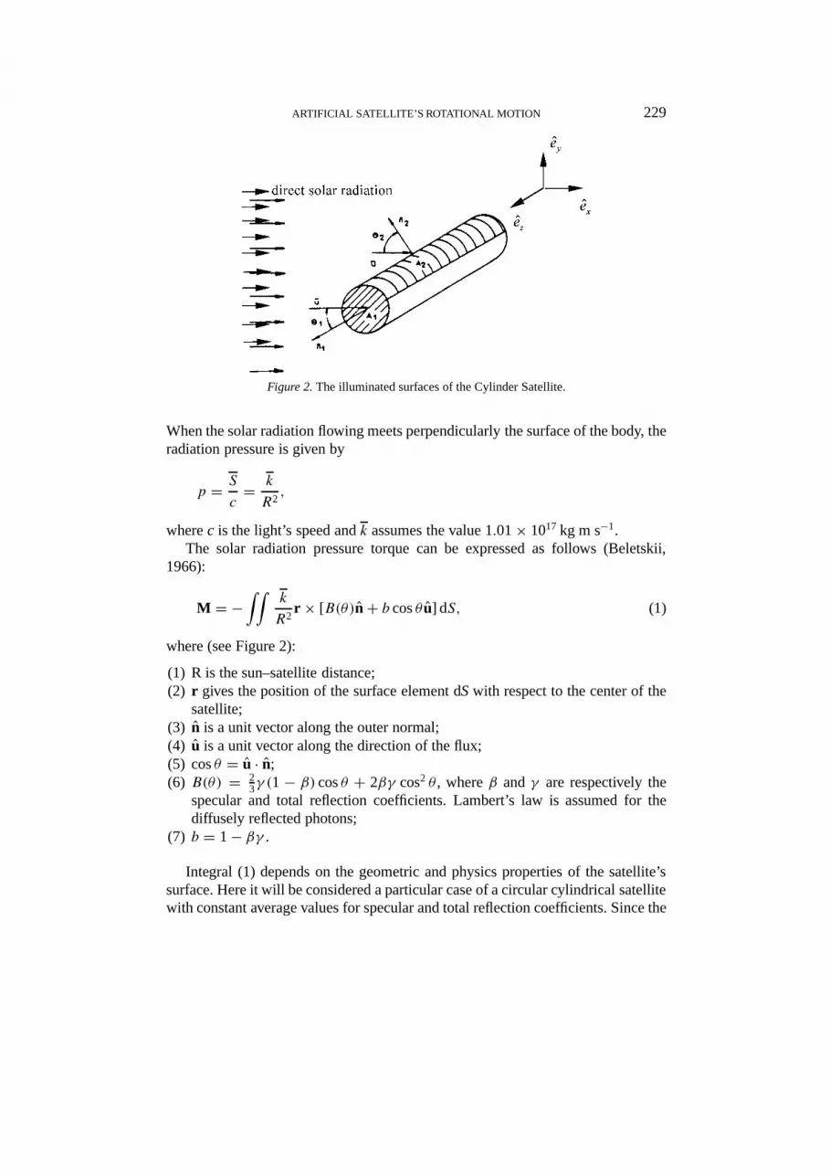
Figure 2.The illuminated surfaces of the Cylinder Satellite.

When the solar radiation flowing meets perpendicularly the surface of the body, theradiation pressure is given by

p = S

c= k

R2,

wherec is the light’s speed andk assumes the value 1.01× 1017 kg m s−1.The solar radiation pressure torque can be expressed as follows (Beletskii,

1966):

M = −∫∫

k

R2r × [B(θ)n+ b cosθ u] dS, (1)

where (see Figure 2):

(1) R is the sun–satellite distance;(2) r gives the position of the surface element dSwith respect to the center of the

satellite;(3) n is a unit vector along the outer normal;(4) u is a unit vector along the direction of the flux;(5) cosθ = u · n;(6) B(θ) = 2

3γ (1 − β) cosθ + 2βγ cos2 θ , whereβ andγ are respectively thespecular and total reflection coefficients. Lambert’s law is assumed for thediffusely reflected photons;

(7) b = 1− βγ .

Integral (1) depends on the geometric and physics properties of the satellite’ssurface. Here it will be considered a particular case of a circular cylindrical satellitewith constant average values for specular and total reflection coefficients. Since the


satellite–earth distance is much smaller than the sun–satellite distance the follow-ing simplifications can be introduced:

(1) The direction of the solar flux is given by the apparent motion of the sun withrespect to the earth;

(2) The sun-earth distance is constant.

The inertial system considered is the equatorial system of the earth and the direc-tion of the solar flux is given as a function of the sun’s right ascension(αs) anddeclination(δs).

The components of the solar radiation torque will be expressed in the system ofthe artificial satellite’s principal axes of inertia (Oxyz with unit vectorsex, ey, ez).This system is related to the inertial system by matrices whose elements are func-tions of the Andoyer’s variables. Therefore, the direction ofu is given by (Zanardi,1993):

u = uxex + uyey + uzez,where

ux = cosδs{cosαs[(cosl2 cosl3− sinl3 sinl2 cosI ) cosl1++ [cosJ (− sinl2 cosl3− cosl2 sinl3 cosI )+ sinJ sinI sinl3] sin l1] ++ sinαs[(cosl2 sinl3 + sinl2 cosl3 cosI ) cosl1++ [cosJ (cosI cosl3 cosl2− sinl3 sinl2)− sinJ sinI cosl3] sin l1]} ++ sinδs{sinI sinl2 cosl1+ (cosJ sinI cosl2+ sinJ cosI ) sinl1},

uy = cosδs{cosαs[(sinl3 sinl2 cosI − cosl2 cosl3) sinl1 ++[cosJ (− sinl2 cosl3− cosl2 sinl3 cosI )+ sinJ sinI sinl3] cosl1] ++ sinαs[(− cosl2 sinl3 − sinl2 cosl3 cosI ) sinl1++ [cosJ (cosI cosl3 cosl2− sinl3 sinl2)− sinJ sinI cosl3] cosl1]} ++ sinδs{− sinI sinl2 sinl1+ (cosJ sinI cosl2+ sinJ cosI ) cosl1},

uz = cosδs{cosαs[(sinJ sinl2 cosl3+ (sinJ cosI cosl2+ cosJ sinI ) sinl3] ++ sinαs[sinJ (sinl3 sinl2− cosI cosl3+ cosl2)− cosJ sinI cosl3]} ++ sinδs{cosI cosJ − sinJ sinI cosl2},

and

cosI = L3

L2, cosJ = L1

L2.

The illuminated surfaces of the cylinder satellite are a circular flat surface(A1),with radiusσ , and the portion of the cylindrical surface(A2), of heightH, as shownin Figure 2.βj andγj , j = 1, 2, are respectively the coefficients of specular andtotal reflection of the surfacesAj .


Cylindrical and polar coordinates can be used to describe the position of thesurface elements with respect to the geometric center of the satellite (Zanardi,1992).

After integration Equation (1) remains (Zanardi, 1993):

M = Mx ex +My ey, (2)

where

Mx = −muyuz, My = muxuzwith

m = k

R2

πσ 2H

2(β2γ2− β1γ1). (3)

For the considered model, as we can see by Equation (2), the solar radiationtorque’szcomponent is zero.

3. Equations for the Rotational Motion

The equations for the rotational motion of a cylindrical type artificial satellite,considering gravity gradient and solar radiation torque, can be expressed in thefollowing form:

dlidt= ∂F

∂Li+ Piψ, dLi

dt= ∂F

∂li+ Siψ, i = 1, 2, 3. (4)

Here(1) F is the Hamiltonian for the conservative problem. The Hamiltonian con-

tains terms up to the order of inverse of the cube of the distance from the satellite tothe earth and terms of the second order in eccentricity. Therefore, the HamiltonianF, for a cylindrical type satellite, can be written in the following form (Zanardi,1986):

F = F0(L1, L2)+ F1(lk, Lk), k = 1, 2, . . . ,6, (5)

where

F0 = 1

2

{[1

C− 1

2A− 1

2B

}]L2

1+1

2

[1

A+ 1

B

]L2

2

}, (6)

F1 = 1

4

(1

B− 1

A

)(L2

2− L21) cos(2l1)+

+(µ4M6

L64

)[2C − A− B

2h1(lk, Lk)] + A− B

4h2(lk, Lk)

], (7)

with


(a) M is the mass of the satellite;(b) µ is the earth’s gravitational constant;(c) A, B, C are the satellite’s principal moments of inertia;(d) lj andLj represent Delaunay’s variables forj = 4,5,6, which describe the

translational motion;(e) h1 andh2 are functions oflkandLk, k = 1,2, . . . ,6. These functions, ex-

pressed in terms of the mean anomaly, were developed in a previous paper(Zanardi, 1986).

Note that the term

1

4

(1

B− 1

A

)(L2

2− L21) cos 2l1

was included in the perturbed HamiltonianF1. This can be true for a cylindricaltype satellite when the moment of inertiaA is not exactly the same as the moment ofinertiaB. (2)Pi andSi are functions of the solar radiation torque components withrespect to the Andoyer variablesli andLi (Zanardi, 1992). For a cylindrical typesatellite these expressions are given in the Appendix. (3)ψ is the shadow-functionintroduced by Ferraz-Mello (1972).ψ is zero if the satellite is in the earth’s shadow,and equals one in the opposite case.

Although refined models are available to describe physically and geometricallythe entry and the exit of an artificial satellite to the earth’s shadow (Kabelac, 1988;Vokroulicky, 1993), Ferraz-Mello’s one provides a good enough approximation forour needs.

In this paper we will obtain an analytical solution for the rotational motionEquations (4) consideringA ≈ B and that the satellite is illuminated, so thatψ =1, When the effect of the earth’s shadow is considered, we will obtain a semi-analytical solution.

4. Canonical Transformation

First we note that, the equations for the torque free rotational motion of a triaxialsatellite was completely solved by Kinoshita (1972) in terms of elliptical functions.

For a cylindrical type satellite, whenPi = Si = 0, the problem is described bythe equations

dlidt= ∂F

∂Li,

dLidt= ∂F

∂li, i = 1,2,3, (8)

with the Hamiltonian given by (5).It must be pointed out that we can include, inF0, secular terms due to the gravity

gradient torque. This can be useful as an integrable kernel of Hori solution (Ferraz-Mello, 1996) for a second order solution of the problem in which gravity gradient


torque must be considered with other perturbations. The system with this newHamiltonian will be solved by canonical transformation using Hori–Lie method.

Since the coupling of the translational-rotational motion produces terms of su-perior order (Zanardi, 1986), we will consider known a first order solution forthe translational motion(lj , Lj , j = 4,5,6). Keplerian motion will be used asunperturbed translational motion.

System (8) can be solved by canonical transformation where the new Hamilto-nianF ′ = F ′0+F ′1, is averaged over fast variables and does not contain short periodterms. The generating functionWhas the formW = W1+W2.

According to the Hori–Lie algorithm (Hori, 1966) the first order perturbation inany variablesx can be found from the following formulax = x′ + {x,W }, wherethe symbol{x,W } is used for Poisson bracket.

Appling the first order Hori–Lie algorithm for the system (8), we have

Li = L′i −∂W1

∂l′i, li = l′i −

∂W1

∂L′i, i = 1,2,3. (9)

The new HaminltonianF ′ is given by

F ′(l′k′, L′k) = F ′0+ F ′1, k′ = 3,5,6, k = 1,2,3,4,5,6, (10)

where

F ′0 = F ′0(L′1, L′2) =1

2

{[1

C− 1

2A− 1

2B

]L′21 +

1

2

[1

B+ 1

A

]L′22

}, (11)

F ′1 = limT→∞

1

T

∫ T

0F1(τ )dτ, (12)

and the generating functionW1 is obtained from

W1 =∫

[F1(τ )− F ′1(τ )] dτ. (13)

The parameterτ is introduced through the called Hori’s auxiliary system or Hori’skernel:

dl′idτ= ∂F ′0∂L′i

,dL′idτ= −∂F

′0

∂l′i, i = 1,2,3. (14)

The new equations of motion are given by

dl′idt= ∂F ′

∂L′i,

dL′idt= −∂F

′

∂l′i, i = 1,2,3. (15)

The solution of the auxiliary system (14) is

L′i = constant, i = 1,2,3,


l′3 = constant, l′1 = n10τ + 1′10, l′2 = n20τ + l′20 (16)

with

n10

(1

C− 1

2A− 1

2B

)L′1, n20 = 1

2

(1

A+ 1

B

)L′2. (17)

Therefore, this solution is composed by the torque free rotational motion for thecylindrical type artificial satellite.

Using the HamiltonianF1 given by Equations (7), and the solution (16), we cancomputeF ′1 andW1 from Equations (12) and (13):

F ′1 =µ4M6

2L′64(2C − A− B)

[1+ 3

2

(1− L

′25

L′24

)+ 15

8

(1− L

′25

L′24

)2]×

×(

3

2

L′21L′22− 1

2

){−1

2+ 3

8(1+ θ ′2− θ ′2− 3θ ′2θ ′2− 3

8sin(2I ′)×

× sin(I ′) cos(l′6− l′3)−3

2sin2(I ′) sin2(I ′) cos(2l′6 − 2l′3)

}, (18)

W1 = 1

8

(1

B− 1

A

) [L′22 − L′21

] sin 2l′1n10

+

+ µ4M6

2L′64

[(2C − A− B)h3(l

′j , L

′j )+

(A− B

2

)h4(l

′j , L

′j )

],

j = 1,2, . . . ,6, (19)

whereh3 and h4 are periodic functions which encloselj , j = 1,2, . . . ,6, asarguments of sines (Zanardi, 1983),θ ′ = cosI ′ = L′3/L

′2 and θ ′ = cosI ′ =

L′6/L′5.

The final solution of the system (9) can be expressed in the following form(Zanardi, 1986):

Li = L∗i + δLi, li = l∗i + nit + δli, i = 1,2,3, (20)

whereL∗i and l∗i are constants;ni = ni0 + nig with n10 andn20 given by Equations

(17), n30 = 0. nig is due to the gravity gradient torque, depending on the termβ

computed by

β = µ4M6(2C − A− B)4L6

40

[1+ 3

2

(1− L

250

L240

)][3L2

10

L220

− 1

],

δLi andδli are periodic functions given by

δLj = δLjCP, j = 1,2, δL3 = δL3LP + δL3CP,

δli = δliLP + δliCP, i = 1,2,3.


Here, δLiCP and δliCP are short periodic variations computed from the termW1 of the generating function;δLiLP and δliLP, depending onl3, l6 andLk, k =1,2, . . . ,6, are long periodic variation (due toF ′1). δL3LP is computed by

δL3LP = α1 sin(α2t + α3)+ α4,

where

α1 = (b2− 4ac)1/2

2a, α2 = ±(−v)(−a)1/2,

α3 = arcsin

[2aL30+ b(b2 − 4ac)1/2

]± (−a)1/2vt0, α4 = − b2a ,

a = −4g2

L220

, b = 4KZ0(g2+ L2

20− L250)

L220

,

c = 4(K2X0 +K2

Y0)−(g2+ L2

20− L250

L20

)2

,

v = 3β

8L250

(g2− L2

50− L220

L20

),

t0 is the initial time and the vectorg is the total angular momentum. Att0, g can beexpressed in the inertial systemOXYZas follows:

g= KX0eX +KY0eY +KZ0eZ,

where

KX0 = L50 sinI ′0 sinl60+ L20 sinI0 sinl30,

KY0 = −L50 sinI ′0 cosl60− L20 sinI0 cosl30,

KZ0 = L50 cosI ′0+ L20 cosI0,

I ′ is the orbit inclination. Sign(±) is determined by the relation:

2 sinI0(KX cosl30−KY sinl30) = ±(aL230+ bL30+ c)2.

5. Analytical Analysis

Considering the satellite always illuminated(ψ = 1) and the effects of the gravitygradient and solar radiation torque being, respectively, of first and second orderwith regard to the torque free rotational motion, let us apply Lagrange’s method(Vilhena de Moraes, 1989) in the system (4), using the first order solution (20).Doing it we get

dL∗idt= Si(σ

∗i , L

∗i , αs, δs,m)−

3∑k=1

[Sk∂(δLi)

∂L∗k+ P k ∂(δLi)

∂σ ∗k

],


dσ ∗idt= ni(L

∗i , m)+ P i(σ ∗i , L∗i , αs, δs,m)−

−3∑k=1

[Sk∂(δσ i)

∂L∗k+ P k ∂(δσ i)

∂σ ∗k

], i = 1,2,3. (21)

In the system (21) we have

(a) the transformation,

L∗i = L∗i , l∗i = σ ∗i − ni t, i = 1,2,3,

was introduced in order to eliminate spurious mixed terms (Vilhena deMoraes, 1981);

(b) P i, Si, ni are, respectively, thePi, Si, ni written in the new variablesL∗i andσ ∗i ;

(c) δLi, δσ i are periodic parts of solution without solar radiation torque expressedin terms ofL∗i andσ ∗i ;

(d) the variablesαs, δs andσ ∗i are always present in the right hand of system (21)as arguments of trigonometric terms.

Thus, neglecting coupling terms in the system (21), we get the following equa-tions for the variation of the constantsL∗i andσ ∗i :

dL∗idt= Si(σ

∗i , L

∗i , αs, δs,m),

dσ ∗idt= ni(L

∗i , m)+ P i(σ ∗i , L∗i , αs, δs), i = 1,2,3. (22)

The solution of system (22) can be obtained by the method of successive approx-imations. It’s interesting to analyze the secular variations from the Equations (22).Thus, eliminating the periodic variables(σ ∗1 , σ

∗2 , σ

∗3 , αs, δs) and integrating we get:

L = constant, σi = n∗i t + σ ∗i0, i = 1,2,3, (23)

with

n∗1 = n1+ m cosJ

8L2

(3 sin2 I − 2),

n∗2 = n2− m

8L2

[cos2 J − cos2 I(2+ 3 cos2 J)],

n∗3 = n3− m cosI

16L2

(3 cos 2J + 1),

whereni are theni expressed in terms of theLi, i = 1,2,3 and

cosJ = L1

L2

, cosI = L3

L2

.


In the application of the method of successive approximations it will be con-sidered the solutions (23) to avoid the spurious Poisson terms. The sun’s rightascension(αs) and declination(δs) will be assumed with a linear variation:

αs = nαt + α0, δs = nδt + δ0,

wherenα andnδ are estimated for the initial time and(α0, δ0) are the initial valuesfor (αs, δs).

Then by the application of the method of successive approximations in theEquations (22), the analytical solution is

L∗1 = constant, L∗j = L∗j0+ δL∗j , j = 2,3,

σ ∗i = σ ∗i0+ (ni +1ni)t + σ ∗i , i = 1,2,3, (24)

whereδL∗j , δσ∗i are periodic functions in the variablesσ ∗i , αs, δs; L∗j0, σ

∗i0 are con-

stants given by the initial conditions;ni and1ni are secular terms due to gravitygradient and direct solar radiation torques.

By examining solution (24) we can conclude that solar radiation torque pro-duces secular and periodic variations in the angular variables, and only periodicvariations in the rotational angular momentum and in its projection on the inertialZ axis.

The projection of the rotational angular momentum on thez-axis’ principalinertial axes system is not influenced by the torque derived from the solar radiationpressure.

Therefore the final solution for the rotational motion equations, considering thetorque produced by direct solar radiation(ψ = 1) and the gravity gradient torque,is

L1 = L10+ δL1, Ls = Ls0+ δLs+ δL∗s, s = 2,3,

li = li0+ (ni0+ ni +1ni)t + δli + δl∗i , i = 1,2,3, (25)

where(a) Li0 andli0, (i = 1, 2, 3) are constants depending on the initial conditions;(b) ni0 are mean motions associated to the free rotational motion, beingn30 = 0

(see Equations (17));(c) δli andδLi are periodic functions andni are mean motions associated to the

gravity gradient torque;(d) δl∗i andδLs

i are periodic functions and1ni are mean motions associated tothe torque produced by solar radiation torque. Their analytical expression canbe derived directly from Equations (4) and Appendix, and the1ni are givenby


1n1 = m cosJ0

8L20(3 sin2 I0− 2),

1n2 = − m

8L20[cos2 J0− cos2 I0(2+ 3 cos2 J0)],

1n3 = −m cosI0

16L20(3 cos 2J0 + 1),

(26)

6. Analytical and Numerical Results

In order to analyze orders for the magnitude of the gravity gradient and solar radi-ation torques, and to validate our analytical solution let us consider an hypotheticalsatellite with its orbital and physical characteristics similar to ‘Pegasus A’ satellite(Cochran, 1972). Thus, the following values will be assumed as

A = B = 3.9499× 105 kg m2, C = 1.0307× 105 kg m2,

M = 11,550 kg, m = −4.245× 105 kg m2 s−1,

orbital period= 5778 s, rotational period= 255 s.

The initial conditions for Andoyer’s variables will be taken as

L10 = 0 kg km2 s−1, l10 = l20 = J0 = π2 rad,

L20 = 9.7307× 10−3 kg km2 s−1, l30 = 5.87 rad,

L30 = −2.9956× 10−3 kg km2 s−1, I0 = 1.887 rad,

The orbit parameters are

e = eccentricity= 0.01617, l40 = 0 rad,

a = semi-axis= 6.95964× 103 km, l5 = 0 rad,

I = 0.5533 rad, l6 = π/6 rad.

A numerical integration was performed by Bulirsch–Stoer method (Bulirsh andStoer, 1966) with time step of 0.1 s and simulation time of 100,000 s (about 20orbital periods and 400 satellite rotations). The used accuracy was EPS= 10−14,with double precision and 10 extrapolation steps.

From the Astronomical Almanac (1993), the following values can be taken (on4 December):

nα = 2.1956× 10−7 rad/s, α0 = 4.3692 rad,

nδ = −2.6767× 10−8 rad/s, δ0 = −0.3876 rad.

The proposed analytical solution and numerical solution are shown in Figure 3 for99,000–100,000 s and in Figure 4 for 0–100,000 s. They agree quite well duringall the considered time.


Figure 3. Andoyer’s variables variations due radiation torque, where1L2 = L2 − L20,

1L3 = L3−L30,1l1 = l1− l10− (1/C−1/A)L10 t,1l2 = l2− l20− (L20/A) t,1l3 = l3− l30.


Figure 4. Andoyer’s variables variation due to solar radiation and gravity gradient torques, where1l2 = l2− l20− (L20/A) t,1l3 = l3− l30,1L3 = L3− L30.

Figure 3 shows the results for all Andoyer’s variables obtained when only solarradiation torque is considered. Due to the choice of the initial conditions (J0 =90◦), l1 has only periodic variation due to the solar radiation torque. The appar-ent secular variation of1L3, as shown in this figure, actualy is a long periodicvariation produced by terms ofS3 independent ofl1andl2 (see Appendix). It mustbe observed that it was consideredA = B in the example. The magnitude of theeffects due to the solar radiation torque in the variations of Andoyer’s variables,during 100,000 s, are 10−7 kg km2s−1 for L3, 10−10 kg km2s−1 for L2, 10−8 rad forl1, and 10−5 rad forl2 andl3.

Table I shows the magnitude of the effects of the solar radiation torque on eachAndoyer’s variables. This table shows also the comparison between the analyticaland numerical solutions, when only the solar radiation torque is considered.


TABLE I

Magnitude of solar radiation torque effects on Andoyer’s variables

Variable Results Time(s)

1000 10000 100000

1L2 Analytical 0.153389× 10−10 −0.574003× 10−9 −0.278858× 10−9

(kg km2s−1) Numerical 0.153796× 10−10 −0.573602× 10−9 −0.274960× 10−9

Difference −0.000407× 10−10 −0.000401× 10−9 −0.003898× 10−9

1L3 Analytical −0.663991× 10−8 −0.673028× 10−7 −0.652717× 10−6

(kg km2s−1) Numerical −0.664114× 10−8 −0.674245× 10−7 −0.665144× 10−6

Difference 0.000123× 10−8 0.001217× 10−7 0.012427× 10−6

1l1 Analytical 0.381969× 10−7 −0.432905× 10−7 −0.301335× 10−7

(rad) Numerical 0.381982× 10−7 −0.432789× 10−7 −0.299838× 10−7

Difference −0.000013× 10−7 −0.000116× 10−7 −0.001479× 10−7

1l2 Analytical −0.764686× 10−6 −0.748143× 10−5 −0.757318× 10−4

(rad) Numerical −0.764803× 10−6 −0.747178× 10−5 −0.748017× 10−4

Difference −0.000117× 10−6 −0.000965× 10−5 −0.009301× 10−4

1l3 Analytical 0.108697× 10−6 0.135434× 10−5 0.136946× 10−4

(rad) Numerical 0.108682× 10−6 0.135311× 10−5 0.135789× 10−4

Difference 0.000015× 10−6 0.000123× 10−5 0.001157× 10−4

Figure 4 shows the results for all Andoyer’s variables when we consider thesolar radiation and gravity gradient torques.L2 has only periodic variations due tothe solar radiation torque since in this case the mean Hamiltonian is considered.Due to the initial conditions the behavior of the variablesl1 andL2 is the samewhen just the radiation solar torque is considered. Concerning the apparent secularvariation of1L3, it can be explained by the long periodic terms considered in thegravity gradient torque. The order of the magnitude in 100,000 s is 10−3 kg km2s−1

for the periodic variations inL3, 10−1 rad forl3 andl2.For a cylindric satellite, Runge–Kutta and Adams–Moulton–Bashforth meth-

ods, beside Bulirsch–Stoer method, were also used to integrate the equations ofrotational motion, when only the gravity gradient torque was considered as a per-turbation. Concerning to the accuracy we have noted that, for this case, all the threemethod lead to the same precision.

7. Semi-Analytical Process

We show here a semi-analytical process to solve Equations (4) when only solarradiation torque and the influence of the earth’s shadow are taken into account.


Figure 5.Mapping of function9’s shadow.

The shadow function9 depends on the parameters of the satellite and the sun’sorbit. In this process a mapping for the function9 is performed and solution (24)is used to compute the variables describing the rotational motion when9 = 1.

The mapping of9 is shown in Figure 5, considering a simulation time of about30,000 s and a satellite whose characteristics are given in Section 5. By this figure,we can observe that, on each orbit, the satellite is on the shadow about 35% of itsorbital period.

The semi-analytical process is given by the following algorithm:

(1) Fromt0 to t1 the satellite is on the shadow and solar radiation torque is zero.

(2) From t1 to t2 the satellite is illuminated and solution (24) is valid, beingt1 the initial time of integration andt2 the final time of integration for thecomputation of the analytical solution in the intervalt1 to t2.

(3) Fromt2 to t3 the satellite is not affected by the solar radiation torque. In thisinterval, the variablesL2, L3, l1 andl3 remain constants, with values fixed att2. Besides the value ofL2 at t2 be different from its value att0, the linearvariation of variablel2 betweent2 andt3 differs from its linear variation in theinterval t0 to t1;

(4) Fromt3 to t4 the satellite is illuminated again and the analytical solution (24)is used, considering the initial condition given int3.

(5) Fromt4 to t5 the satellite is in the earth’s shadow, the procedure is similar toitem 3.

(6) After t5 the procedure will be repeated.


Figure 6. Semi-analytical solution and numerical solution due to solar radiation torque, where1L2 = L2 − L20,1L3 = L3 − L30,1l1 = l1 − l10 − (1/C − 1/A)L10 t,1l2 = l2 − l20−(L20/A) t,1l3 = l3− l30.


The results of this semi-analytical process are shown in the grafics of Figure 6.The semi-analytical solution is compared with a numerical solution of Equation (4)performed by the Bulirsh Stoer method.

8. Conclusions

An analytical solution for the equations describing the rotational motion of anartificial satellite under the influence of the gravity gradient and the solar radiationtorques was presented. A model for solar radiation torque was also developed for acircular cylinder satellite. This solution, valid when the satellite is totally illumin-ated, presents secular terms in all angular variables. The modulus of the rotationalangular momentum and its projection on the inertialZ-axis contain only periodicterms. Due to the symmetry of chosen satellite, the projection of rotational angularmomentum on thez-axis’ principal axis system of inertia is not affected by solarradiation torque and gravity gradient torque.

When compared with a numerical integration the solution shows to be very ac-curate for about 20 orbital revolutions and 400 rotations of an hypothetical satellite.

A semi-analytical procedure was also proposed to predict the satellite’s attitudewhen the earth’s shadow is taken into account. In this procedure a mapping of theshadow’s function is constructed and a known analytical solution is used whenthe satellite is illuminated. The semi-analytical solution was also compared withnumerical integration.

When other torques are also considered, this analytical solution can be usefulas a propagation method in an optimization process of attitude determination.

Appendix

For a cylindrical type satellitePi andSi are given by

S1 = 0

S2 = mK

a2s

{[b1 sin 2l2 + b2 sinl2](3 cos2 δs− 2)+

+ cos2 δs[b3 sin(−2l3 + 2l2 + 2αs)+ b4 sin(−2l3 − 2l2+ 2αs)++ b5 sin(−2l3 + l2+ 2αs)+ b6 sin(−2l3− l2− 2αs)] ++ sin 2δs

2[b7 cos(−l3− 2l2 + αs)+ b8 cos(−l3+ 2l2 + αs)+

+ b9 cos(−l3− l2+ αs)+ b10 cos(−l3+ l2+ αs)]

},

where

b1 = sin2 J sin2 I

4, b2 = −sin 2J sin 2I

8,


b3 = sin2 J

8(2− sin2 I − 2 cosI ), b4 = sin2 J

8(−2+ sin2 I − 2 cosI ),

b6 = sin 2J sinI

8(cosI − sinI ), b7 = −sin2 J sinI

2(cosI + 1),

b8 = sin2 J sinI

2(cosI − 1), b9 = sin 2J

4(cos 2I + cosI ),

b10 = sin 2J

4(− cos 2I + cosI ).

S3 = −mKa2

s

cos2 δs{d1 sin(2l3 + l2− 2αs)+ d2 sin(l2− 2l3 + 2αs)++ d3 sin(2l3 − 2αs)+ d4 sin(2l3 + 2αs)+ d5 sin(2l3+ 2l2 − 2αs)++ d6 sin(2l2 − 2l3+ 2αs)+ d7[sin(2l3 − 2l2 + 2αs)++ sin(2l3+ 2l2+ 2αs)] + d8[cos(−2l3 + 2αs)+ cos(2l3+ 2αs)−− 1

2 sin(2l3 − 2l1 − 2αs)− 12 sin(2l3− 2l1 + 2αs)+

+ 12 sin(2l3 + 2l1 − 2αs)− 1

2 sin(2l3+ 2l1 + 2αs)++ 1

2 cos(2l3+ 2l1 + 2αs)+ 12 cos(2l3 + 2l1− 2αs)+

+ 12 cos(2l3− 2l1 + 2αs)+ 1

2 cos(2l3 − 2l1− 2αs)++ cos(2l3 − 2l2+ 2αs)+ cos(−2l3+ 2l2 + 2αs)++ cos(2l3 + 2l2+ 2αs)+ cos(−2l3− 2l2 + 2αs)] ++ d9[cos(2l3 − l2+ 2αs)+ cos(2l3− l2 − 2αs)−− sin(2l3− l2+ 2αs)+ cos(2l3 + l2+ 2αs)++ cos(2l3 + l2− 2αs)− sin(2l3 + l2+ 2αs)++ 1

2 cos(2l3− l2+ 2l1 + 2αs)+ 12 cos(2l3 − l2+ 2l1 − 2αs)+

+ 12 cos(2l3+ l2+ 2l1 + 2αs)+ 1

2 cos(2l3 + l2+ 2l1 − 2αs)++ 1

2 cos(2l3+ l2− 2l1 + 2αs)+ 12 cos(2l3 + l2− 2l1 − 2αs)+

+ 12 cos(2l3− l2− 2l1 + 2αs)+ 1

2 cos(2l3 + l2− 2l1 − 2αs)−− 1

2 sin(2l3 − l2− 2l1 + 2αs)− 12 sin(2l3 − l2− 2l1 − 2αs)−

− 12 sin(2l3 + l2− 2l1 + 2αs)− 1

2 sin(2l3 + l2− 2l1 − 2αs)−− 1

2 sin(2l3 − l2+ 2l1 − 2αs)+ 12 sin(2l3 − l2+ 2l1 + 2αs)−

− 12 sin(2l3 + l2+ 2l1 + 2αs)− 1

2 sin(2l3 + l2+ 2l1 − 2αs)] ++ d10[sin(2l3+ 2l2 − 2l1 − 2αs)+ sin(2l3 − 2l2 + 2l1− 2αs)++ sin(2l3+ 2l2− 2l1 + 2αs)+ sin(2l3 − 2l2 + 2l1+ 2αs)−− cos(2l3 + 2l2+ 2l1 − 2αs)− cos(2l3− 2l2 − 2l1 − 2αs)−− cos(2l3 − 2l2− 2l1 + 2αs)− cos(2l3+ 2l2 + 2l1 + 2αs)] ++ d11[sin(2l3+ 2l2 + 2l1 − 2αs)+ sin(2l3 − 2l2 − 2l1− 2αs)+


+ sin(2l3+ 2l2+ 2l1 + 2αs)+ sin(2l3 − 2l2 − 2l1+ 2αs)−− cos(2l3 − 2l2+ 2l1 − 2αs)− cos(2l3+ 2l2 − 2l1 − 2αs)−− cos(2l3 − 2l2+ 2l1 + 2αs)− cos(2l3+ 2l2 − 2l1 + 2αs)]} ++ mKa2

s

sin 2δs

2{d12 cos(−l3+ αs)+

+ d13 cos(−l3+ l2+ αs)+ d14 cos(−l3− l2+ αs)++ d15 cos(−l3− 2l2+ αs)+ d16 cos(−l3+ 2l2+ αs)++ d17[cos(l3− 3l2 + αs)− cos(l3+ 3l2 + αs)−− cos(l3− l2+ αs)− cos(l3+ l2+ αs)] ++ d18[cos(−l3− 3l2 + αs)− cos(−l3+ 3l2+ αs]}

where

d1 = −sin 2J

4

(7

16sin 2I + sinI

), d3 = −sin2 I

32(5+ 9 cos 2J ),

d2 = sin 2J

4

(7

16sin 2I − sinI

), d4 = sin2 I

32(3+ 7 cos 2J ),

d5 = − 1

64{sin2 J (16 cosI + 9+ 7 cos 2I )+ 2 sin2 I },

d6 = − 1

64{sin2 J (9− 16 cosI + 7 cos 2I )+ 2 sin2 I },

d7 = 1

16

{1− cos2 I sin2 J + cos2 J

2(sin2 I − 2)

},

d8 = −cos2 J sin2 I

16, d10 = sin2 I

64(cos2 J − cosJ ),

d9 = −sin 2J sin 2I

64, d11 = sin2 I

64(cos2 J − cosJ ),

d12 = sin 2I

8(3 cos 2J + 1), d13 = sin 2J sin 2I

16(1+ 6 sinI ),

d14 = sin 2J

4[2 cos 2I + sin 2I

4(6 sinI − 1)],

d15 = sinI (cos 2J − 1)

8(cosI + 1), d17 = − 1

16sin 2J sin 2I sinI,

d16 = sinI (cos 2J − 1)

8(cosI − 1), d18 = − 1

16sin 2J sin 2I,

P1 = mK

a2s

{[2e1 + 2e2 cos 2l2](3 cos2 δs− 2)+ cos2 δs[e3 cos(−2l3 + 2αs)++ e4 cos(−2l3+ l2 + 2αs)+ e5 cos(−2l3 − 2l2 + 2αs)+


+ e6 cos(−2l3+ 2l2 + 2αs)+ e7 cos(−2l3− 2l2 + 2αs)] ++ sin 2δ2

2[e8 sin(l3− αs)+ e9 sin(l3+ l2− αs)+

+ e10 sin(l3− l2− αs)+ e11 sin(l3+ 2l2− αs)++ e12 sin(−l3+ 2l2 + αs)]}

where

e1 = −cosJ

8L2(3 sin2 I − 2), e2 = −cosJ sin2 I

8L2,

e1 = 3

4

cosJ sin2 I

L2, e4 = −cos 2J sinI

4L2 sinJ(cosI − 1),

e5 = −cosJ

8L2(1+ 2 cosI + cos2 I ), e6 = −cosJ

8L2(1+ cos2 I − 2 cosI ),

e7 = cos 2J sinI

4L2 sinJ(cosI + 1), e8 = −3

2

cosJ sin 2I

L2,

e9 = cos 2J

2L2 sinJ(cos 2I + cosI ), e10 = − cos 2J

2L2 sinJ(cos 2I − cosI ),

e11 = cosJ sinI (1+ cosI )

L2, e12 = −cosJ sinI (1− cosI )

L2,

P2 = mK

a2s

{[f1+ f2 cos 2l2 + f3 cosl2](3 cos2 δs− 2)++ cos2 δs[f4 cos(−2l3 + 2αs)+ f5 cos(−2l3+ 2l2 + 2αs)++ f6 cos(−2l3 − 2l2+ 2αs)+ f7 cos(−2l3 + l2+ 2αs)++ f8 cos(−2l3 − l2+ 2αs)++f9(cos(−2l3+ 3l2 + 2αs)− cos(2l3 − 3l2 + 2αs))] ++ sin 2δs

2[f10 sin(−l3+ αs)+ f11 sin(−l3+ l2 + αs)+

+ f12 sin(−l3− l2+ αs)++ f13 sin(−l3+ 2l2+ αs)+ f15 sin(−l3− 2l2+ αs)++ f14[sin(l3+ 2l2 + αs)+ sin(l3− 2l2+ αs)] ++ f16(sin(l3+ l2+ αs)+ sin(l3− l2+ αs)+ sin(l3+ 3l2 + αs)++ sin(l3− 3l2+ αs))++ f17[sin(l3+ 3l2 + αs)+ sin(−l3− 3l2+ αs)]]},

where

f1 = 1

4L2[cos2 J (1− 6 cos2 I )+ cos2 I ],


f2 = 1

4L2[cos2 J (1− 2 cos2 I )− cos2 I ],

f3 = 1

16L2{sin 2I [sin 2J − 4 cotJ cos 2J ] + 2 cotI sin 2J (3 sin2 I − 2)},

f4 = 1

4L2[cos2 J (cos2 I − 3 sin2 I )+ cos 2J cos2 I ],

f5 = 1

8L2(1− cosI )[cos2 J − cosI cos 2J ],

f6 = 1

8L2(cosI + 1)[cos2 J + cosI cos 2J ],

f7 = 1

4L2

[(cosI − 1) cotJ cos 2J sinI +

+ cotI sin 2J

8(−4+ 8 cos2 I − 3 cosI )

],

f8 = 1

4L2

[(cosI + 1) cotJ cos 2J sinI +

+ cotI sin 2J

8(−4+ 8 cos2 I + 3 cosI )

],

f9 = 1

32L2cotI sin 2J cosI,

f10 = 1

4L2{−6 cos2 J sin 2I + cos 2I cotI (3 cos 2J + 1),

f11 = 1

2L2

{cosI

[sin 2J

2cos 2J cotJ

]+

+ cos 2I cotJ cos 2J − 7

4cos2 I sin 2J

},

f12 = 1

2L2

{cosI

[cos 2J cotJ − sin 2J

2

]+

+ cos 2I cotJ cos 2J − 7

4cos2 I sin 2J

},

f13 = 1

L2

{cos 2J sinI + cotI

4(cos 2J − 1)(cos 2I − cosI )

},

f14 = 1

4L2sin 2I cos2 J,

f15 = 1

L2

{− cos2 J sinI + (cos 2J − 1)

cotI

4(cosI + cos 2I )

},

f16 = 1

8L2cos2 I sinJ, f17 = 1

8L2cos2 I sin 2J,


P3 = mK

a2s

{(3 cos2 δs− 2)[g1 + g2 cosl2+ g3 cos 2l2 + g4 cos 3l2] ++ cos2 δs[g5[cos(−2l3+ l2+ 2αs)+ cos(−213 − l2+ 2αs)] ++ g6 cos(−3l3+ 2αs)++ g7 cos(−2l3+ 2l2 + 2αs)+ g8 cos(−2l3− 2l2 + 2αs)] ++ sin 2δs

2[g9 sin(−l3+ αs)+ g10 sin(−l3+ 2l2 + αs)+

+ g11 sin(−l3− 2l2 + αs)++ g12 sin(−l3− l2+ αs)+ g13 sin(−l3+ l2+ αs)++g14(sin(l3+ l2+ αs)+ sin(l3− l2+ αs)+ sin(l3 − 3l2+ αs)++ sin(l3− 3l2+ αs))++ g15 sin(−l3+ 3l2 + αs)+ g16 sin(−l3− 3l2+ αs)]},

where

g1 = cosI

8L2(1+ 3 cos 2J ),

g2 = − 1

16L2 sinI(sinJ sin2 I − 4 sin 2J cos 2I ),

g3 = cosI

16L2(cos 2J − 1), g4 = −sinI sinJ

16L2,

g5 = sin 2J

16L2(2 cos2 I − 5 sin2 I ), g6 = sin 2I

16L2(3 cos 2J + 1),

g7 = sinI

16L2[2 sin2 J + cosI (1+ 3 cos 2J )],

g8 = sinI

16L2[−2 sin2 J + cosI (1+ 3 cos 2J )],

g9 = − cos 2I

2L2 sinI(cos 2J + cosJ ),

g10 = 1

4L2 sinI[(cos 2J − cosJ )(cos 2I − cosI )+ sin 2J sinI ],

g11 = − 1

4L2 sinI[(cos 2J − cosJ )(cos 2I + cosI )− sin 2J sinI ],

g12 = sinJ

4L2[cosI (6 cosJ + 1)+ 1],

g13 = sinJ

4L2[(cosI (6 cosJ + 1)− 1],

g14 = sin 2J sinI

16, g15 = sinJ

4L2(1− cosI ), g16 = −sinJ

4L2(cosI + 1).


References

Belestkii: 1966, NASA TF – 429.Bulirsh, R. and Stoer, J.: 1966,Numerishe Mathematik8, 93–104.Cochran, J. E.: 1972,Celest. Mech. & Dyn. Astr.6, 127–150.Ferraz-Mello, S.: 1982,Celest. Mech. & Dyn. Astr.5, 80–101.Ferraz-Mello, S.: 1996,Celest. Mech. & Dyn. Astr.66(1), 39–50.Georgeovic, R. M.: 1973,J. Astr. Sci.XX (5), 255–274.Hori, G.: 1966,Publ. Astr. Soc. Jap.18, 287–295.Kabelac, J.: 1988,Bull. Astr. Inst. Czechosl. 39, 213–220.Kinoshita, H.: 1972,Publ. Astr. Soc. Jap.24, 423–457.Vilhena de Moraes, R.: 1981,Celest. Mech. & Dyn. Astr.25, 281–292.Vilhena de Moraes, R.: 1989,Celest. Mech. & Dyn. Astr.45, 281–284.The Astronomical Almanac: 1993, U.S. Government Printing Office, Washigton, D.C.Vokroulicky, D., Farinella, P. and Mignard, F.: 1993,Astron. Astrophys.280.Wiggins, L. E.: 1964,AIAA J.4, 271.Zanardi, M. C.: 1983,Movimento Rotacional-Translacional Acoplados de Satélites Artificiais,

Master Thesis, ITA, São José dos Campos, SP, Brazil.Zanardi, M. C.: 1986,Celest. Mech. & Dyn. Astr.39, 147–158.Zanardi, M. C. and Moraes, R. V.: 1992,Proc. 32nd Annual Israel Conference on Aeronautics and

Astronautics, pp. 279–286.Zanardi, M. C.: 1993,Influencia do Torque de Radiaçao Solar na Atitude de um Satélite Artificial,

Doctoral Thesis, ITA, São José dos Campos, SP, Brazil.Zanardi, M. C. and Moraes, R. V.: 1994,J. Brazilian Soc. Mech. Sci.XVI , 533–535.

ABCAnalytical and semi-analytical analysis of an artificial satellite’s rotational motion

Documents

Transcript of ABCAnalytical and semi-analytical analysis of an artificial satellite’s rotational motion