Semi-Analytical Galaxiesin the

MultiDark UniverseA perspective on the evolution of the most luminous

and massive galaxies throughout cosmic history

A dissertation submitted in partial fulfilment of therequirements of the degree of

Doctor of Philosophy in Theoretical Physics

of the Universidad Autónoma de Madrid

by

Doris Stoppacheradvised by

Dr. F. Prada & Dr. A. Knebe

Madrid, November 2019

ii

Abstract

Understanding the formation and evolution of galaxies within a self-consistent cosmologicalcontext is one of the outstanding and most challenging topics of astrophysics. This dissertationis dedicated to investigating the concepts of galaxy formation with cosmology, in particular, theformation of large-scale structures and the assembly and evolution of their associated galaxiesover cosmic time. This forms part of a vibrate and innovative field of research spanning allimaginable scales from The Big Bang to the Milky Way Galaxy with its many satellites.

Over the last few decades a lot of effort has been invested into the development of models whichcan produce statistically significant sets of galaxy properties in a computationally efficient way.These models included the population of dark matter halos using simplified phenomenologicaltreatments of baryonic processes and coarse-graining the properties of galaxies. As a result,relevant equation systems can be solved more efficiently – a semi-analytical model (SAM) wasborn.

The MultiDark-Galaxies was an ambitious project dedicated to the release of galaxycatalogues from three different SAMs: Galacticus, SAG, and SAGE; run on the MultiDarkPlanck 2 N-body simulation covering a cubic volume of 1h−1Gpc as part of this thesis work.To this point, the released galaxy catalogues remain one of the largest of their kind based onSAMs. We perform a comparison of the outputs of the three models and their conformity withfundamental galaxy properties derived from observations. Each model of galaxy formation hasits unique recipe followed by individual calibration and tuning, therefore we highlight theirdifferences and similarities. We demonstrate further that SAMs are an exceptional resourcefulmethod of studying statistically significant samples of galaxy properties.

We identify modelled galaxies from Galacticus, which show similar properties as observationalsamples and therefore are truly comparable with luminous red galaxies (LRGs) from e.g. SDSS atz ∼ 0.1 or BOSS-CMASS at z ∼ 0.5. We extract CMASS-mock samples from Galacticus usingthe original photometric selection as well as alternative methods mimicking such a selection. Westudy these mock samples in detail and find correlations of properties related to star formation:(specific) star formation rate, gas-phase metallicity ZCold, and cold-gas fraction MCold/M∗, butalso properties such as the halo mass M200c or the black hole mass MBH; with the large-scalestructure environment e.g. filaments or knots.

We emphasise that, the bimodalities found in the properties of Galacticus’ CMASS-mocks,manifesting themselves as two distinct populations, could provide insights in the galaxy evolutionin the context of the origin of the fundamental luminosity/mass-metallicity relation, merger-induced star formation, or “downsizing”. Our results may further challenge the paradigm thatthe large-scale environment does not influence the galaxy formation and predictions on theevolution of a galaxy inside its halo can be derived only from the halo mass and the occupationdistribution, also know as the galaxy assembly bias.

We trace the progenitors of Galacticus’ LRG-samples at low redshift to z ∼ 0.5 and identify20% of them as CMASS. We show further the full mass growth history of the progenitors ofthe most diverse populations, red and blue, found in the CMASS-mock of Galacticus. Wefind that those samples have distinct properties, cluster differently, and have been assembled atdifferent cosmic times, most probably throughout different evolutionary paths. We will conductfurther analyses in order to confirm the possible detection of a galaxy assembly bias signal inour SAM.

iii

iv

Resumen

Comprender la formación y evolución de las galaxias dentro de un contexto cosmológico auto-consistente es uno de los temas más destacados de la astrofísica actual y uno de sus mayoresretos. Esta tesis está dedicada a investigar los conceptos de formación de galaxias en una cos-mología distinca, y en particular a la formación de estructuras a gran escala y al ensamblaje yevolución de las galaxias asociadas a las mismas a lo largo del tiempo cósmico. Esto forma partede un campo de investigación vibrante e innovador que abarca todas las escalas imaginables,desde el Big Bang hasta la Vía Láctea con sus numerosos satélites.

A lo largo de las últimas décadas se ha invertido mucho esfuerzo en el desarrollo de modeloscapaces de producir conjuntos estadísticamente significativos de propiedades de galaxias de unamanera computacionalmente eficiente. Estos modelos han incluido la población de halos demateria oscura utilizando tratamientos fenomenológicos simplificados de procesos bariónicosy procesar rudimentario las propiedades de las galaxias. Como resultado se ha obtenido unaresolución más eficiente de los sistemas de ecuaciones relevantes, lo que ha supuesto el nacimientodel modelo semi-analítico (SAM).

El proyecto The MultiDark-Galaxies es un ambicioso proyecto dedicado a la obtenciónde catálogos de galaxias de tres SAM diferentes: Galacticus, SAG y SAGE; ejecutado enla simulación de N -cuerpos MultiDark Planck 2 cubriendo un volumen cúbico de h−1Gpccomo parte de este trabajo de tesis. En la actualidad, los catálogos de galaxias publicados siguensiendo algunos de los más grandes de su tipo basados en SAM. Realizamos una comparación delos resultados de los tres modelos y de su concordancia con las propiedades fundamentales de lasgalaxias derivadas de las observaciones. Cada modelo de formación de galaxias usa presciptionesúnicas, así como calibraciones y ajustes individuales, por lo que podemos analizar sus diferenciasy similitudes. Además, demostramos que los SAM son un método excepcionalmente ingeniosopara estudiar muestras estadísticamente significativas de propiedades de galaxias.

Identificamos galaxias modeladas por Galacticus que muestran propiedades similares a lasmuestras observacionales y que son comparables con las galaxias rojas luminosas (LRG) decatálogos como SDSS en z ∼ 0.1 o BOSS-CMASS en z ∼ 0.5. Extraemos muestras simuladas deCMASS de Galacticus utilizando la selección fotométrica original, así como métodos alter-nativos que imitan dicha selección. Estudiamos estas muestras simuladas de forma detallada yencontramos correlaciones entre propiedades relacionadas con la formación estelar: tasa de for-mación de estrellas (específica), metalicidad en fase gaseosa ZColdy fracción de gas frío (MCold/M∗), pero también con otras propiedades como la masa de halo M200c o la masa del agujeronegro MBH; con el entorno de galaxias a gran escala, por ejemplo filamentos o nudos.

Cabe resaltar que las bimodalidades encontradas en las propiedades de la muestra similadaCMASS de Galacticus, que se manifiestan como dos poblaciones distintas, podrían propor-cionar información sobre la evolución de la galaxia en el contexto del origen de la relaciónfundamental luminosidad / masa-metalicidad, la formación estelar producida por mergers, o“downsizing”. Nuestros resultados pueden desafiar aún más el paradigma de que el entorno agran escala no influye en la formación de galaxias y las predicciones sobre la evolución de unagalaxia dentro de su halo pueden derivarse solo de la masa de halo y la distribución de ocupación,también conocida como el sesgo de ensamblaje de galaxias.

Rastreamos los progenitores de las muestras LRG de Galacticus con un desplazamiento al rojobajo hasta z ∼ 0.5 e identificamos el 20% de ellos como CMASS. Mostramos además el historialcompleto de crecimiento en masa de los progenitores de poblaciones muy diversas, rojas y azules,

v

que se encuentran en la muestra similada de CMASS de Galacticus. Encontramos que esasmuestras tienen propiedades distintas, se agrupan de manera diferente y se han ensambladoen diferentes tiempos cósmicos, muy propablemente siguiendo diferentes caminos evolutivos.Llevaremos a cabo más análisis para confirmar la posible detección de una señal de sesgo deensamblaje de galaxias en nuestro SAM.

vi

Contents1 Introduction 1

1.1 Part I: How does the Universe work? . . . . . . . . . . . . . . . . . . . . . . . . . 11.1.1 A brief introduction on the history of the Universe . . . . . . . . . . . . . 11.1.2 Galaxies – A Universe’s accomplishments . . . . . . . . . . . . . . . . . . 51.1.3 The galaxy-halo connection . . . . . . . . . . . . . . . . . . . . . . . . . . 71.1.4 The Large-Scale Structure & Environment . . . . . . . . . . . . . . . . . . 10

1.2 Part II: How to simulate a Universe on a computer? . . . . . . . . . . . . . . . . 121.2.1 Galaxy formation theory . . . . . . . . . . . . . . . . . . . . . . . . . . . . 131.2.2 Modelling techniques in galaxy formation . . . . . . . . . . . . . . . . . . 141.2.3 Semi-analytical models (SAMs) . . . . . . . . . . . . . . . . . . . . . . . . 16

1.3 Part III: Modern challenges in galaxy formation & evolution – The Assembly Bias 20

2 Thesis Overview 232.1 Overview & Introduction of the MultiDark-Galaxies as Thesis Compendium . . . 232.2 Publications & Authorship on the MultiDark-Galaxies . . . . . . . . . . . . . . . 24

3 Paper I – The MultiDark-Galaxies 27

4 Paper II – Luminous red galaxies and their correlation with environment 55

5 Paper III – The Three Hundred Clusters 73

6 Main Results on the MultiDark-Galaxies 936.1 The MultiDark-Galaxies and their distinctiveness . . . . . . . . . . . . . . . . . . 936.2 Galaxy properties reflected in the clustering performance . . . . . . . . . . . . . . 936.3 Quiescent galaxies in the spotlight – Luminous giants and their relation to their

dark matter halos . . . . . . . . . . . . . . . . . . . . . . . . . . . . . . . . . . . . 946.4 Nature vs. nurture? - Environment as a factor to be considered . . . . . . . . . . 966.5 A million ways to simulate a galaxy cluster . . . . . . . . . . . . . . . . . . . . . 97

7 Conclusion & Discussion of the Main Results on the MultiDark-Galaxies 99

8 Conclusión & Discusión de los Resultados Generales de las The MultiDark-Galaxies107

Bibliography 115

vii

1 IntroductionI am fascinated! When I was very young and took a look onto the bright night sky, I wasfascinated. When I learned, that all those sparkling stars, I observed, are actually suns thatlived a long time ago in systems far away from us, I was fascinated. Much later, when I found outthat, each tiny temperature anomaly measured in the cosmic microwave back ground radiation(CMB) [218] is about to grow towards the impossible size of a supercluster and gives rise tothe most massive objects in the Universe, I was fascinated. And finally, when I researched thecosmic history and galaxy evolution for this very dissertation, I have been truly fascinated. Iam fascinated by the puzzles the Universe holds for us, by the mechanisms of galaxy formation,by the formation and growth of structure, by the question where did we come from and whereare we heading for, I was always fascinated.

With that fascination in my head and mind, I am going to introduce theories of galaxy evolutionand computational methods of galaxy formation with the main objective of understanding whatdoes shape galaxy properties in a cosmological context. In the first part of this introduction, abrief review of the most important paradigms of cosmology and the history of the Universe isgiven, before focusing on luminous red galaxies and their connection to their dark matter halos.The second part is dedicated to the presentation of modelling techniques and introduces mainlysemi-analytical models of galaxy formation and evolution. In the third and last part of thisintroduction, one example of modern challenges in the field of galaxy formation is presented –the assembly bias, which recently has been a topic for extensive debate.

1.1 Part I: How does the Universe work?

The Universe is all of time and space,1 born from The Big Bang, driven by late-time acceleration[220, 231], and constrained by the fundamental laws of nature such as conservation, classicalmechanics, and relativity [308]. The Universe comprises all energy and matter in their variousforms as an isolated2 thermodynamical system steadily pursuing the maximisation of its ownentropy according to the second law of thermodynamics.3

1.1.1 A brief introduction on the history of the Universe

In the framework of modern cosmology and astrophysics, the standard model, Lambda Cold DarkMatter (ΛCDM) [41, 91, 257], describing the formation and evolution of the cosmos, is builtupon two simple but important principles supported by a number of observations [139, 155, 221]:The Universe is isotropic and homogeneous [100, 128], although we find ourselves living in avery inhomogeneous place, a galaxy. Our galaxy, the Milky Way, forms part of an even largerstructure, a network of galaxies, clusters, and superclusters we call the cosmic web [34], wheregalaxies are aligned on rather thin filaments and concentrated towards the centre of gravitysuch as huge knots hosting the most massive clusters and galaxies. For an illustration of theobservable Universe see Fig. 1.1.

1 ... everywhere and anywhere, every star that ever was. Where do you want to start? – Doctor Who2 However, if the Universe is really a closed system remains controversy [117].3 The second law of thermodynamics states that the entropy of an isolates system can never decrease over time,but reaches its maximum in the state of thermodynamical equilibrium [47]

1

1 Introduction

The expansion and evolution of the Universe is determined by the Friedmann Equations [107],derived from Einstein’s field equation in the context of general relativity4 and the under assump-tion of the cosmological principle. The solution for a flat open world model can be expressedin one single elegant equation and describes the evolution of the cosmic scale factor 5 (a) withtime and therefore the expansion of the Universe:

H2(t) =

(a

a

)2

= H20 [Ωrad (1 + z)4 + Ωm (1 + z)3 + Ωk (1 + z)2 + ΩΛ] (1.1)

with H0 being today’s Hubble constant and the Ωs, the density parameters defined as the ratioof the observed density ρ to the critical density6 ρcr of today’s Universe. z is the redshift of theUniverse and related to the scale factor as a(t) = 1/(1 + z). The density of radiation is givenby Ωrad, the density of matter by Ωm, the density of curvature by Ωk, and the density of darkenergy 7 by ΩΛ, respectively:

Ωrad =8πG

3 H20

ρrad , Ωm =8πG

3 H20

ρm , Ωk = − c2

H20

k , ΩΛ =c2

3 H20

Λ (1.2)

with G being the gravitational and Λ the cosmological constant.8

The density parameter given in Eq. (1.1) such as radiation or matter scale differently withredshift z. Therefore, each component of the equation dominates the expansion of the Universeat different cosmological times. Each transition, when one of the parameters started dominatingthe expansion, brought forward a new era in cosmic history. Currently, the energy densitycorresponding to the dark energy, represented by ΩΛ is dominating and causing what we calllate-time acceleration. Dark energy took over the expansion of the Universe almost at the sametime as the solar system formed or the first tracers of life appeared on Earth (a coincidence?!).Before this epoch, the Universe went through a phase where collisionless dark matter togetherwith ordinary baryonic matter, represented by Ωm, dominated its fate. Previously, baryonshave not yet been cool enough to accrete into the potential wells of the cold dark matter toform galaxies. The obscure period of time, where the Universe has been transparent,9 but nostar was born yet, is called dark ages. The only photons which could travel freely throughspace and time originated from the cosmic microwave background radiation (CMB), the oldestobservable of the Universe at z ∼ 1100. The CMB consists of photons which could escape theircoupling state and have not experienced an interaction with matter ever since. Previously tothe time of recombination, where the Universe actually became transparent, the temperature

4 Spacetime tells matter how to move; matter tells spacetime how to curve – John A. Wheeler, theoretical physicist5 The scale factor is a dimensionless parameter which represents the relative expansion of the universe and relatesthe comoving distances for an expanding universe with the distances at a reference time – the present.

6 The critical density is estimated to be approximately 5 atoms/m2 whereas the average density of baryonic matterseems to be approximately 0.2 atoms/m2 [230]. Furthermore, the contribution to the total energy budget of theUniverse is with ∼ 5% fairly small [221].

7 It is distinguished from ordinary matter in the sense that is has a negative pressure. It holds ∼ 70% of theUniverse’s total energy budget, but its true nature or origin has not been identified yet [48, 215, 237]. It furtherprovides a general label on physics which is unknown or currently not well enough understood [8].

8 Originally introduced by Einstein in his field equation to guarantee for a static solution for the Universe and sincethe 1990s associated with the energy of the vacuum as the simplest explanation of dark energy. As Amendola andTsujikawa [8] noted in their book, coincidently Aristotle first proposed an “eternal” and “incorruptible” cosmicsubstance in The Lambda Book (i.e. the 12th) of his Metaphysics.

9 That means that the photons could propagate without getting scattered on or re-emitted by baryons.

2

1.1 Part I: How does the Universe work?

was to high to allow atoms to recombine into their neutral states. This epoch is know as theradiation-dominated phase where the driving component of the equation of expansion aroundredshift z ∼ 3400 was Ωrad and the baryons and photons tightly coupled to each other in a statewhich is comparable to that of a hot dense plasma. With the nucleosynthesis [32] finishing thebuild-up of the basic elements: hydrogen, deuterium, and helium10; approximately at minute 3of cosmic time or z ∼ 108, we enter the era of the early Universe. The evolution of the Universeand its properties had already been predestinated by its phase transitions most probably a resultof spontaneous symmetry breaking .11 The predominance of matter over antimatter during theBaryogenesis, an example of symmetry breaking, left us with a baryonic 12 fine-tuned 13 Universedestined to bring forward life.14 Our knowledge of the physics before that is very incomplete. Weonly can assume that primordial density perturbations seeded the cosmic structure formationduring an episode of extreme expansion called inflation 15 [3, 125, 267]. During the earliest epochof the Universe, the Planck era, the laws of physics, as we understand them today, might nothave even been applicable since the fundamental forces still have been unified and the Universe’sstate comparable with a chaotic foam of quantised black holes,16 space and time inextricablyand discontinuously, unimaginable by a human mind.17 And finally all that was initialised byThe Big Bang.

The ΛCDM paradigm, described in the most straightforward way above, provides a generalframework allowing galaxies to form and evolve. Thereby large-scale structure is dominated bycollisionless, dissipationless cold dark matter which forms potential wells in which the baryonscan accrete, cool, and subsequently form proto-galaxies. The physical mechanisms involved inthis process are described by the framework of galaxy formation and evolution and includesroughly gas cooling, star formation, and feedback processes (which will be described in detail inwhat follows). In the next section, we will focus on the end product of those processes: Galaxies.They are the objects on the smallest scale we discuss in this thesis. We will then subsequentlymove to larger scales when introducing the interaction of galaxies with their dark matter halos,their clustering dependency, and their environmental affiliation.

10We, all of us, are what happens when a primordial mixture of hydrogen and helium evolves for so long that itbegins to ask where it came from. – Jill Tarter, astronomer

11It describes the spontaneous process of a symmetric state to end up asymmetrically and is a common phenomenonseen in particle physics such as the (Nobel prize winning) charge conjugation parity symmetry (CP)-violation[53].

12Physicists are made of atoms. A physicist is an attempt by an atom to understand itself. – Michio Kaku,theoretical physicist

13It seems that dimensionless physical constants such as the strength of the electromagnetic interaction betweenelementary charged particles, commonly known as the fine-structure constant 1/α ∼ 137 [127, 261] have tightlyconstrained values. Small variation in them would make structure formation or nuclear fusion and therefore life,as we know it, non-existent.

14A controversial explanation for the observed fine-tuning of the Universe uses the anthropic principle whichbasically states that the properties of the Universe and hence fundamental constants must be compatible withthe establishment of intelligent life to observe it [14, 49]. Interestingly, the fine-tuning problem as well as theanthropic principle have been debated interdisciplinary for more than 100 years (also compare to puddle thinking[2]). Richard Feynman once said that every theorist should have the following statement written on their officeboard: “1/137, how little we know? ” [108]. In his honour, I chose the font size of this dissertation to be 11.37pt.

15Originally proposed in the early 1980s to solve several cosmological problems such as the flatness or horizonproblem, provides a casual mechanism for the origin of large-scale structures in the Universe [8].

16As described by John A. Wheeler17Never limit yourself because of others’ limited imagination; never limit others because of your own limited imag-ination – Mae Jackson, astronaut

3

1 Introduction

©Pab

loCar

los

Bud

assi

Figure 1.1: Logarithmic scale illustration of the observable Universe.

4

1.1 Part I: How does the Universe work?

1.1.2 Galaxies – A Universe’s accomplishments

The above described expanding Universe luckily brought forward a diversity of objects we callgalaxies. They are dynamically bound systems which consists of a variety of material such ascold and hot gas, stars, metals, black holes, and dark matter.

Fundamental properties of galaxies

Galaxies come in many different shapes and sizes. They can be divided into distinct populationssuch as red and blue, old and young, metal-rich and metal-poor, elliptical and disk. For thisthesis work, we only need to understand the overall characteristics of the most massive luminouspopulation, which are know to be redder, older, and can be found in the most massive structures[258]. In this section, we review briefly common terms used in the framework of galaxy formationand evolution and the most important properties of galaxies:

• Stellar masses: The stellar mass is one of the most important properties of a galaxyand can be used as a proxy for other properties as we will see in Chapter 4 of thisthesis. The abundances of galaxies as a function of mass is given by the stellar massfunction (SMF ). Galaxies seem to build up their mass continuously over cosmic time [183].Thereby, their characteristic number densities follow the shape of a Schechter-function[243]. Massive galaxies formed and assembled their stars earlier than lower massive galaxieswhich synthesised their stellar masses later and over longer periods of time [202, 206]. Inthis work we are mostly interested in massive quiescent galaxies.

• Luminosities and colours: The luminosity is the total amount of electromagnetic en-ergy emitted per unit time while its flux is the rate of energy transferred per unit surfaceor wavelength/frequency. The colour of an astrophysical object can be described roughlyas the difference in flux/energy/magnitude measured by certain band-pass filters of a pho-tometric system. The luminosity-colour distribution of a sample of galaxies is stronglybimodal [11] with the majority of galaxies being located in a quite narrow optical wave-length range know as the red sequence and in a slightly broader blue cloud. In the localUniverse, the red sequence was found to host predominantly quiescent galaxies showinglow rates of star formation and older stellar populations, whereas the blue cloud’s pop-ulations are younger and their galaxies are actively starforming. The bimodality in theluminosity-colour or colour-colour diagram provides deep insights into the evolution of agalaxy population. We will us the colour of galaxies in order to select a galaxy sample byapplying photometric selection cuts Chapter 4.

• Number densities: The comoving number density of quiescent galaxies increases withtime since the cosmic noon 18 [39], while the number of starforming galaxies has been moreor less constant [206]. This implies that, with time the star formation in galaxies becomeless and less efficient or has be suppressed, which we call quenching. Number densitiesare useful to our analysis, since we will later show how to mimic a photometric selectionusing the same number density of objects of its observational counterpart. The quenchingof star formation is further important to this thesis when discussing if ant to what degreeenvironment shapes galaxy properties in Chapter 7.

• Scaling relations: The tight correlations of galaxy properties, also called scaling rela-tions, have been intensively studied in the past. They help to classify galaxies according

18The peak of cosmic star formation and black hole accretion around z ∼ 2 − 3 [183]

5

1 Introduction

to their morphology type such as disk or elliptical, size and growth, or prominent featuressuch as spiral arms as well as give clues about their intrinsic properties. Diverse scal-ing relations e.g. for dwarf galaxies revealed that the mechanisms behind the formationof these objects are actually different from the formation of normal-sized galaxies [157].Scaling relation are important in the framework of galaxy formation, as we will see later,since they can be used to implement physical processes at the sub-grid19 level and consistof the most direct approaches to constrain baryon cycling processes. Some examples forscaling relations are:

– The cold gas fraction is the fraction of the cold gas MCold in the interstellar medium(ISM) to the total stellar mass M∗ [12, 216]. The gas fraction decreases since cosmicnoon and is assumed to tightly correlate with star formation history and the cold gasdensity [223].

– The mass-metallicity relation describes the relation of the metallicity or masses ofmetals of the stars or in the ISM to the total stellar mass [280, 304]. Its evolutionsuggests that galaxies of a given stellar mass M∗ had lower cold gas-phase metallitiesZCold at higher redshift [304] and that galaxies which form stars more rapidly havesubsequently lower metallicities [168, 185]. We will come across this relation manytimes when presenting our results, since our adopted model of galaxy formation,introduced in Chapter 3, shows dependencies of properties related to star formationand ZCold on their large-scale environment (spoiler!).

– The fundamental plane is a combination of properties such as radius, luminosity, andvelocity of galaxies based on the classic Faber-Jackson relation [101] or Kormendyrelation [156] for elliptical and Tully-Fisher relation [281] for disk galaxies. Therebythe galaxies populate a fairly narrow region in the luminosity-radius-velocity plane.

– The stellar-to-halo mass relation is one of the tightest relations and provides usefulinformation on the formation and evolution of a galaxy of given halo and stellarmass within its dark matter halo. Interestingly, the halos at intermediate massesproduce most efficiently stars [22, 38, 296]. It is still poorly understood why haloswith lower or higher masses form stars by orders of magnitudes less efficiently. [17].Furthermore, this relation is crucial to our research, because we want to understandthe evolution and the large-clustering of luminous red galaxies living in the mostmassive halos.

– Recent studies have shown that there is a fairly tight correlation between secondarygalaxy properties such structural parameters or colour and the properties of darkmatter, apart from the stellar mass. In what follows we will discuss the galaxy-haloconnection in detail in Section 1.1.3 and introduce modelling approaches of how toparametirisise this important scaling relation in Section 1.2.2.

Luminous Red Galaxies (LRGs)

As mentioned before, LRGs are our main research object in this thesis. Here we will summarisetheir most important properties. They are located in the centre of dense regions as today’scluster and supercluster and therefore hosted by the most massive dark matter halos [176]. Theyserve as powerful cosmological probes to study the formation of structure, the assembly of mass

19Those are the small-scale physical processes that occur at length-scales beyond resolution limits or act as a placeholder for not yet understood physics.

6

1.1 Part I: How does the Universe work?

and cosmology itself. However, their detailed formation and evolution is still not sufficientlyunderstood or quantified [274, 291]. To shed light on the topic one would need informationabout the full history of mass assembly and star formation of luminous red galaxies within alarge redshift range. The Baryon Oscillation Spectroscopic Survey [hereafter BOSS, 88, 99, 244]provides such data.

The BOSS-CMASS galaxy sample of luminous red galaxies

The Sloan Digital Sky Survey (hereafter SDSS) III, also known as BOSS, was dedicated to study-ing properties of the large-scale distribution of massive galaxies. The BOSS sample is divided intoa low (LOWZ) and a high redshift sample (CMASS, stands for “constant mass”), respectively. TheCMASS-sample was designed to target the most luminous red galaxies in order to produce a inmass uniformly distributed sample of ∼ 1.5 million LRGs. The sample exhibits a peak comovingnumber density n ∼ 3.4× 10−4 h3Mpc−3 at z ∼ 0.5 and shows only passive evolution with littleor no on-going star formation [186] along the redshift range of 0.43 < z < 0.7. The galaxies areselected by applying a set of photometric selection cuts20 using (g-i) and (r-i) colours, where g,r, and i stand for the bands of the classic photometric filters of the SDSS. An important charac-teristic of this colour selection is that it guarantees for an extension towards the bluer colours,hence blue-cloud galaxies can enter the sample. Because the CMASS sample consists of a non-evolving population of massive galaxies, it provides an excellent “cosmic laboratory” to studygalaxy formation and evolution [25, 197, 198] as well as their link to cosmology via e.g. theirspatial distribution and clustering [122, 234]. BOSS LRGs were repeatedly used to determinefundamental cosmological parameters [77, 111], to probe cosmological models [4, 29, 203], andto inform the relation between the dark matter halos to their hosted galaxies [104, 121, 211]. Wededicated a great deal of our analysis to CMASS-galaxies and will show how and how successfulwe can select the same galaxy population from a model of galaxies formation in Chapter 4.

Galaxy Formation in a cosmological context

The amount of mass detectable by human astrophysical instrumentation in the form of baryonsis only about 1/5 of the total mass budget the Universe holds [221]. The remaining 4/5 can onlybe measured indirectly due to the alignment and behaviour of galaxies in the gravitational fieldof their underlying dark matter distribution. Studying the basic properties of galaxies changednot only our entire view of the Universe, as it has been discovered that galaxies live in halos ofdark matter [239], but also the fact that their properties and evolution are tightly linked theirhalos [291] has been an unexpected discovery of modern astrophysics. The so called, galaxy-halo connection is a fundamental and highly complex relation incooperating many physicalprocesses, some of them possibly not even discovered yet. Exploring this relation is crucialto our understanding of galaxy formation and evolution and helps in finding an answer to thefundamental question of what shapes the observables of galaxies.

1.1.3 The galaxy-halo connection

In the framework of cosmology, the galaxy-halo connection relates multivariate distributions ofproperties of dark matter halos with their galaxies. Getting to the bottom of this relation wouldnot only help in understanding the physics of galaxy formation, but also probe the propertiesand the distribution of the underlying dark matter [291]. The most challenging questions in this

20See the BOSS target selection web page for details on the photometric selection cuts https://www.sdss.org/dr15/algorithms/boss_galaxy_ts/

7

1 Introduction

context is: Which properties of dark matter halos and their environment are most significantlyshaping properties of galaxies or in other words How do halo properties induce star formationor quenching in their galaxies?

Early works on the galaxy-halo relation recognised that more massive galaxies and clustersshould also show different clustering statistics than average galaxies, merely because their darkmatter halos exhibit such a strong clustering dependency on halo mass [86, 143, 195]. Therealisation of large survey missions of galaxies in the 90s of the last century made it possible tomeasure huge sets of galaxies simultaneously (e.g. with Two-degree Field Galaxy Redshift Survey[59] or SDSS [302]). The field of computational astrophysics grew quickly with the developmentof N -body simulations [58, 160] being able to resolve substructures of dark matter halos. Bothdisciplines together allowed for detailed studies on the galaxy-halo relation, here we summarisetheir most important findings:

• Scaling of stellar and halo mass: The stellar mass, M∗, of a given galaxy scales withhalo mass, MHalo, as M∗ ∼MHalo

2−3 for dwarf stellar masses and with M∗ ∼MHalo1/3 at

the highest stellar masses [178]. The shape of the stellar-to-halo mass function (SHMF ),derived from the mismatch between the halo mass function and the galaxy stellar massfunction (SMF ), provides evidence for strong feedback processes in galaxy formation whichresults in actively suppressing the star formation.

• Feedback: Typical feedback processes can be observed in galaxies with high and lowhalo masses such as induced by an active galactic nucleus (AGN) in high-mass galaxies[74, 251], or by supernovae of massive stars in low-mass galaxies [89, 136]. Both preventthe gas from cooling and limit star formation.

• Star formation efficiency: It exists a maximum efficiency in the star formation of agalaxy depending on its stellar mass, located around the mass of the Milky Way Galaxy(M∗ ∼ 1012 M), and a narrow range in halo mass where galaxies most productively formstars [17, 63].

• Bias: The bias factor b represents the ratio of the clustering of galaxies in comparisonto their underlying matter distribution: b2 = ξgal/ξDM , ξgal and ξDM are the two-pointcorrelation functions of galaxies and dark matter, respectively [143]. Lower mass halos havean almost constant bias, meaning that, they follow tightly their underlying dark matterdistribution. Halos of higher masses are less abundant, have a larger scatter in SHMF atfixed halo mass, σlog10M∗ , and as a result, are stronger clustered [306]. Furthermore, theirbiases rise quickly with halo mass.

• Concentration is a halo property that informs about the distribution of the dark matterinside a halo. It is defined as c ≡ rhalo/rs with rhalo being the radius of the halo estimatedby a certain over-density criterion,21 and rs the typical scale radius.22 The concentrationis closely related to the formation time and mass assembly (see also mass-concentrationrelation [147, 226]) of a halo as well as the evolution of the galaxy residing in it [68, 240,292, 293, 311]. To mentioned a few examples: halos which experienced a recent merger

21Since the dark matter halos have no strict dimensions, rhalo and subsequently the mass inside the halo need tobe defined via a certain over-density criterion as e.g. the radius at which the gravitationally collapsing spherevirialises (rvir) or when the density inside the radius reaches 200 × the critical density of the Universe (r200ρcr)[194]

22The slope of the density slope coincides with that isothermal sphere, r−2, at rs. The density profile seems tobe universal for a wide range of halo masses and variants of the curvature density parameter Ωk (see Eq. (1.1))[207]

8

1.1 Part I: How does the Universe work?

are low-concentrated, while high-concentrated halos are older and had longer phases ofquiescent evolution. Furthermore, more concentrated halos tend to host more massivecentral galaxies and are also stronger clustered. They start to host the central at lowerhalo masses than less concentrated halos [307].

The scatter in the stellar-to-halo mass relation

The basic shape of the SHMF provides strong evidence of feedback mechanisms driving theformation and evolution of galaxies. Feedback can be found on almost all scales and in all typesof galaxies as its strength depends not only on halo mass, but also on redshift and environment.The scatter in the SHMF , given as the variation of stellar mass at fixed halo mass, σlog10M∗ ,is another important feature of the galaxy-halo connection in central galaxies. It basicallycharacterises the mean value of stellar mass in bins of halo mass, indicating that a galaxies witha fixed mass can live in halos of different masses. This applies fundamental constrains on both,the galaxy and halo properties, most responsible for star formation, quenching, and/or theirtransformation into quiescent galaxies. The scatter σlog10M∗ shows the following dependencies:

• At low masses, the scatter has a constant value but widens considerable due to the changein the slope of the SHMF (see e.g. Fig. 5 in Wechsler and Tinker [291]).

• Above the pivot mass (the halo mass which corresponds to the maximum in star formationefficiency MHalo ∼ 1012), the scatter is monotonically increasing.

• As σlog10M∗ increases, the mean halo mass at fixes stellar mass decreases

• The higher the scatter, the shallower the mean stellar mass increases with halo mass.

• If the scatter is lower, galaxies with higher stellar masses can be found in halos of lowermasses.

It is important to bear in mind that, the variation of the scatter affects directly the clusteringof galaxies, since with increasing σlog10M∗ , the halo mass that permits to host a galaxy witha certain stellar mass decreases with the scatter. In other words, an increasing scatter makesmore low-mass halos to host galaxies with the same mean stellar mass as more massive halos.Since high-mass halos cluster stronger and are also more biased, the clustering signal of samplesselected by stellar mass would show deviations depending on the scatter. We explained thegalaxy-halo connection and the scatter in such detail in this section, because later in Chapter 4(spoiler!) we will show that our adopted model of galaxy formation and evolution shows notsufficient scatter in its SHMF . This has consequences on the halo occupation distribution (theprobability of a halo of certain mass to host a certain amount of galaxies) and subsequently onthe clustering performance of our selected galaxy sample.

Measurements on the scatter are reported in the literature as e.g. 0.18 < σlog10M∗ < 0.22 [314]at z = 0.0 using SDSS galaxies or σlog10M∗ = 0.18 [275] using BOSS at z = 0.5.

The clustering of galaxies

The clustering signal of galaxies, measured as the two-point auto-correlation function (hereafter2pCF), holds fundamental information about the structure formation of the Universe. It is notonly a powerful cosmological probe constraining the matter density parameter Ωm, observationsalso have shown that the clustering results depend strongly on luminosity, morphology, andother physical properties of a given galaxy sample [85, 90, 210]. The 2pCF is defined as the

9

1 Introduction

measurement by counting and averaging the number of neighbours of each galaxy at a givenscale, compared to a random distribution. This gives the typical shape of the clustering functionof e.g. the baryon acoustic oscillations (BAO) measured by BOSS, where at a certain scale, thelength of the sound horizon ∼ 100 h−1 Mpc, an excess in number density of galaxies can befound. This scale serves as a standard ruler and important cosmological constraint, since itdescribes the maximal distances photons could travel before decoupling from the hot, denseplasma of electrons and baryons at the time of recombination. The resulting sound waves areimprinted in the CMB power spectrum. The signal of the BAO is used for accurate distantmeasurements and to constrain cosmological parameters [171].

The evolution of the stellar-to-halo mass function

Does the galaxy-halo relation evolve with redshift? As we have discussed in this section, halo andgalaxy properties are closely correlated. It would be interesting to know, if this relation holdsat higher redshift or if a redshift-dependent factor can be derived. That information would giveclues on how strongly the mass assembly of a galaxy depends on its halo mass. As mentionedbefore, the star formation efficiency correlates highly with mass, but weakly with redshift [17].Behroozi et al. [16] found that the SHMF evolves only little with the peak of the relation nearlybeing constant until z ∼ 3. However, not enough evidence was brought forward yet to supportthe hypothesis that the slope of the SHMF changes significantly with halo mass and redshift.

1.1.4 The Large-Scale Structure & Environment

In the framework of galaxy formation it is vital to understand if the large and small scaleenvironments influence the properties as well as their evolution of a given sample of galaxies[31, 95, 212, 290]. The correlation between galaxy properties and galaxy environment has beenstudied for almost 100 years with the result that many galaxies cannot be found in isolation,but are members of gravitationally bound larger structures. It further has been proven that,elliptical galaxies prefer cluster environments, whereas spirals the field (morphology-densityrelation) [94].

What is environment? In the field of galaxy formation and evolution, the term environmenthas been used differently depending on the context: It could be referred to as the interactionbetween satellites and centrals [241], but it could also be understood in terms of the “groupenvironment” like the distance from the centre of a cluster or defined by its surface density[181, 190]. Other studies refer to environment as the location of a galaxy within the large-scale structure distribution[158, 219, 295] which can be roughly divided into four categories:knots/nodes, filaments, sheets, and voids [126, 175]; in consequence of the hierarchical structureformation [78].

Galaxy Clusters

The large-scale distribution of galaxies in the Universe is dominated by the endeavour of galaxiesto group into clusters and superclusters. Galaxy clusters are the largest gravitationally boundobjects and therefore consist of excellent laboratories to study galaxy formation and evolution.Many recent works have been presented on galaxy clusters [51, 84, 112] as well as many groupsformed dedicating their research effort on their modelling and simulation: e.g. the nIFTy galaxyclusters [79], Cluster-EAGLE [9], The Three Hundred[80], or the MultiDark-Clusters[305], only to mention a few of them.

10

1.1 Part I: How does the Universe work?

The formation of clusters strongly depends on the applied cosmology, but also on the variouscomplex feedback processes, regulating and shaping galaxy properties or determine their mor-phology as e.g. early-type galaxies can often be found in denser environments [94]. Therefore, wededicate this section to the discussion of feedback driven environmental processes that impactcluster galaxies.

Feedback processes and properties of cluster galaxies are tightly correlated with each other,which makes them difficult to entangle. On top of that, clusters have their own characteristicsregarding their formation. In the framework of halo formation, clusters grow in an inside-out manner in two growth phases, a “fast” growth phase of the central region driven by rapidaccumulation and major merger events followed by a “slow” phase, where the outer regionsgradually grow via moderate matter accretion [120]. As a result, the internal structure of haloscontain information about their growth history [73, 292], which can then be used to trackdifferences in the evolutional paths of cluster members.

It is important to understand, if some galaxy or halo properties determine the evolution of clustergalaxies (or the whole cluster) rather than others, and if the local and large-scale environmentplay a role in this scenario. For example, the most significant effect environment has on clustergalaxies is the gas stripping in outer regions of the cluster, resulting in a systematic differencein effective radius and leading to the transformation of their morphology type (e.g. from theblue cloud to the red sequence) [36, 92]. Recent works have also shown that, possibly the smallscale environment influences the evolution of cluster galaxies more than the large-scale [181].Other works studied X-ray emission from clusters and found a significant offset of the locationof the central galaxy, most likely a bright cluster galaxy (BCG), with respect to the centre ofthe X-ray emission peak[115].

Why are galaxy cluster relevant to our discussion? The BCG consist of another sample ofluminous galaxies, although their properties are similar to those of “normal” LRGs [60, 192], theyenable galaxy formation studies in the visual and X-ray range of the electromagnetic spectrum(see e.g. the COSMOS survey [61, 129, 246]). The paradigm that, central galaxies are also the mostmassive in the system, has been proven as not being entirely correct by recent works [255].23

Suspicious offsets of central galaxies with respect to the centre of the halo have also been foundin model clusters in The Three Hundred [80] derived from semi-analytical models. SinceBCGs can be found in denser environments, they would also provide a promising additionalresearch object to the BOSS LRGs (our main research object in this thesis) and possibly help onour mission to trace the galaxy assembly bias. However, this would be beyond the scope of thisdissertation, therefore we leave the studies of clusters and cluster galaxies with respect to theirenvironment for future works.

We summarise that, baryons occupy only a small fraction of the total energy budget of theUniverse and dominate at small scales such as inside a galaxies, inside a host halo as e.g. theinteraction between centrals and satellites, or within groups and clusters of galaxies. In general,feedback processes such as gas cooling or AGN activity regulate the star formation in galaxiesand therefore influence basic properties such as their morphological type or colour. Feedbackis one of the most important and at the same time at least understood mechanism within theframework galaxy formation, since it involves a variety of processes and also is strongly linkedto the host environment of a given galaxy.

23Speaking of paradigms and biases, the same leading author of this publication also wrote an interesting and veryrelevant article on women in physics see Skibba [254]

11

1 Introduction

Quenching and feedback

The phenomenon that the star formation of a certain galaxy is very rapidly ceased is calledquenching [5, 39, 72]. The existence of a tight connection between the quenching and feedbackprocesses is widely accepted, but it seems that different mechanisms are at work for differentpopulations of galaxies. In the low stellar mass range, feedback from massive stars typicallydrives the quenching [72, 82, 169]. In more massive galaxies M∗ > 1 × 1010 Mthe feedback ofthe central AGN is powerful enough to heat up the surrounding cold gas by injecting energy viaradio jets as well as to remove the gas content in the ISM of the galaxy through outflows andwinds [74]. This type of quenching is referred to as mass-quenching, mostly depending on thestellar mass and usually found in central galaxies [217].

A more complex process is the environmental-quenching where the interaction between galaxiesand their surroundings, e.g. if the galaxy is a cluster of group member, quench the star formation[279]. Common phenomena thereby are: ram-pressure stripping [120, 222], strangulation [170,201], and harassment [102, 200]; and most likely to be found in satellite galaxies.

Until now it is not entirely clear what exactly causes the quenching and to what degree itinvolves properties such as morphology or environment. To discuss a few examples, Wanget al. [288] confirmed a weak but significant dependency on environment, but reported that theprimary driver for quenching is halo mass which regulates the star formation in both, centralsand satellites. Other works as e.g. Contini et al. [65] found that the star formation stronglydepends on stellar mass, rather than environment or halo mass. A few studies have found thatit is more likely for galaxy to be quenched or red, if it is hosted by more massive halos [205],but other studies have shown that there is only little dependence on either the halo mass or thedistance from the central galaxy.

Summary: In this section we provided the necessary background to study luminous red galaxyby discussing their basic properties such as mass, morphology, or scaling relations. We furtherestablished a connection between the galaxies and their dark matter halos which consists ofa fundamental relation. We further argued about the influence of their small- and large-scaleenvironments and presented examples of studies from the literature derived from models andobservations. In summary, it is well established that galaxies in denser environments are older,redder, metal-richer, more concentrated, more luminous, and show higher surface brightnessthan galaxies in voids. However, the formation of structures due to the spherical collapse andthe virialisation of dark matter halos as well as the accretion of baryons into these halos andthe subsequent formation of galaxies involve non-linear and highly complex processes whichcannot be described analytically anymore. Therefore, modern computational techniques arenecessary to investigate in detail the processes involved. In what follows, we introduce modellingtechniques of galaxy formation and evolution and will provide a brief overview of cutting-edgemethods and subsequently centre our discussion on semi-analytical models.

1.2 Part II: How to simulate a Universe on a computer?

In this section we introduce cosmological simulations of galaxy formation and evolution in formof a short presentation of the galaxy formation theory as well as the most common modellingtechniques and their ingredients. Since the development of the first cosmological simulations inthe early 80s, the field has grown ever since. Modern research in astrophysics and cosmologycannot be imagined without using computational approaches anymore. The knowledge accu-mulated over almost 40 years helps to complete our view of the Universe and provide crucial

12

1.2 Part II: How to simulate a Universe on a computer?

insights informing other field as observational cosmology or astronomy. Both domains, compu-tation and observation together, form the baseline for cosmological studies and cannot succeedone without the other. Galaxy formation depends highly on observations, because they providethe necessary constraints modellers use to calibrate or tune their models. The challenges andthe ultimate objective of models are to reproduce the observed Universe as detailed and accurateas possible.

1.2.1 Galaxy formation theory

The theory of galaxy formation consists of the modelling of physical processes that affect thebaryonic component distributed in their dark matter halos. It can be separated into two steps:(i) modelling the formation and evolution of the halo population hosting the galaxies using N -body simulations or analytical methods like the Press-Schechter theory [227] and (ii) modellingthe evolution of the baryonic matter distributed in their halos [70].

Overview of physical processes involved in galaxy formation and evolution

• Gravity: Provides the “skeleton” for galaxy formation and determines the shape andamplitude of the primordial power spectrum of density fluctuation, described by the initialconditions and the applied cosmology. The evolution of the power spectrum and thereforethe growth of structure via merging and accretion of halos is predicted by the framework ofhierarchical structure formation. The number and properties of dark matter halos existingin the simulation as well as their evolution is recorded in the so called merger trees.

• Cooling: After the skeleton of dark matter has been formed, gas will accreted into theover-dens regions and eventually cool down. Thereby, we can roughly distinguish threecooling regimes: bremsstrahlung (Tgas ∼> 107 K), cooling via recombination of electronswith ions (104 < Tgas < 107 K), and metal line cooling through collisional excitation/de-excitation of heavy elements and molecules (Tgas < 104 K).

• Star formation: The gas cooled down enough to collapse into the deepest potential wellusually the central region of the halo. It might become self-gravitating and collapse evenmore rapidly driven by its own mass rather than by the dark matter halo. Eventually,denser regions form and will reach temperatures and pressures to enable nuclear fusionand star formation. In this discussion, we describe star formation only rudimentarily,since many processes involved are still poorly understood and simulations are unable toresolve the relevant scales. Therefore, empirical sub-grid recipes, a standard procedurein large-scale cosmological simulations, are introduced to fill in for the lack of physicalunderstanding or resolution.

• Feedback can be classified as thermal (heating the gas), kinetic (ejecting the gas due towinds), and radiative (ionising or photo-dissociating the gas). It regulates the cooling ofgas and subsequently the star formation in galaxies. As we briefly raised the subject inthe previous section, it can be discriminated between: supernova feedback (such as photo-heating, photo-ionisation, winds [136]) and AGN feedback (mostly in early-type galaxiesand in the majority of all massive galaxies as they seem to host a central black hole [157]).The latter is associated with high-velocity winds and cold gas ejection from the interstellarmedium of the galaxy into the hot halo [131]. Both feedback processes are also treated assub-grid implementation in current cosmological simulations.

• Mergers: In the ΛCDM paradigm large-scale structures form hierarchically via halos

13

1 Introduction

merging into more massive and more concentrated objects [55]. The merging events clearlyaffect the galaxies hosted by the merging halos through triggering star formation, changingtheir morphology types, or disrupting and accreting one another. It can be discriminatedbetween minor and major mergers. In the standard scenario, it is assumed that duringa major merger the disk of the central is destroyed and all stars migrate to a spheroidalbulge. Picturing the formation of early-type galaxies in this way is fairly simple and inpractice is more complicated and therefore needs careful modelling, hence some modellerse.g. track the mass loss from satellites when moving through the dark matter halo orassume dynamical friction, the loss of momentum and kinetic energy through gravitationalinteraction e.g. in a system hosting central and satellite galaxies [52].

• Chemical evolution plays an important part in galaxy evolution, because metal line-cooling at intermediate temperatures and subsequent star formation is boosted by metal-rich gas. The luminosity and colour of stellar populations are also highly sensitive tometallicity, since heavy elements produce dust that reddens the galaxy in the ultra-violetand optical as well as re-radiates energy in the infrared [62].

1.2.2 Modelling techniques in galaxy formation

In this section, we introduce modelling techniques in modern computational astrophysics andcosmology. We will briefly summarise the most popular approaches and then focus on semi-analytical models as most relevant to our work.

Empirical models: Some modelling techniques are called empirical, because they map ob-servable properties of galaxies onto properties of dark matter halos, but do not include actualmodelling of physical processes. The most basic approach is called halo abundance matching(HAM). It assumes that the most massive dark matter halo also hosts the most massive galax-ies, while the second most massive halo hosts the second most massive galaxy (and so forth)[141, 161, 234]. This approach is famous for its “non-parametric” implementation, meaning thatthere is at least only one parameter necessary to constrain the model, usually the scatter of theSHMF , σlog10M∗ . A more sophisticated approach is called halo occupation distribution (HOD)and describes the galaxy-halo connection as the mean number of galaxies per halo <Ngal> asa function of MHalo, passing a particular observational selection [24, 235, 312]. There are manydifferent parameterisations available usually using a set of 5-10 parameters. The conditionalluminosity/mass function (CL/MF) goes one step further and describes the full distributionof galaxy luminosity or stellar masses for a given halo mass (The luminosity or stellar massfunction is “conditioned” on the halo mass) [69, 284, 298]. It further can be used to not onlyparameterise the galaxy-halo connection, but e.g. the relation between galaxy star formationrates and halo mass accretion rates [291].

We summarise that, empirical models have fairly simple assumptions, which do not hold whenconsidering e.g. feedback processes we discussed in the previous section. However, empiricalmodels as simple as they are, they are predicting the galaxy-halo connection remarkably well.Furthermore, they are very helpful in determining the galaxy formation histories or generatingmock galaxy catalogues [16, 233].

Physical models: We can roughly distinguish between three types of physical models: N -body, hydro-dynamics, and semi-analytics; although the approaches can be mixed or one buildupon the other (e.g. N -body+hydro). The first step consists of choosing a cosmological modelsuch as ΛCDM and applying initial conditions. Those can contain random perturbations in

14

1.2 Part II: How to simulate a Universe on a computer?

a homogeneous density field of the dark matter distribution, random seeds of particles in thesimulation box, or mimic e.g. the over-densities in the local Universe [286].

Numerical N-body dark matter only simulations

N -body methods, also named “gravity-solvers”, establish the dark matter structure in cosmo-logical simulation by discretely computing the forces between dark matter particles in the fieldof gravity. That basically means solving the Poisson’s equation. The evolution of the systemis followed within a co-moving expanding cosmological frame using periodic boundaries. Theexpansion is derived from the Friedmann-Equations (obtained from the field equations of gen-eral relativity) or a Newtonian approximation of that, since general relativity corrections arenegligible on large scales. This approach is widely used to model large-scale structure formationin a cosmological context and was used for the first time by von Hoerner [287] 1963 to describethe dynamics of stellar clusters.

N -body methods can also include baryons. Such simulations are either particle-based 24 suchas MultiDark [147] or Euclid-Flagship [225], mesh-based 25 such as Millennium [265],or hybrids of both. Particle- and grid-based methods have advantages and disadvantages e.g.particle-based codes can introduce a softening length, the length between two particle where thethe gravitational interaction is suppressed, while mesh-codes are limited by the resolution oftheir grids. Therefore, hybrid tree-mesh codes have been developed using the particle approachon large scales and the mesh approach on small scales in order to resolve those more accurately.A popular example for a hybrid-code is Gadget-2/3 [262].

In the context of galaxy formation, two fundamental properties are given by the underlyingdark matter structure: the distribution of their masses at a certain redshift as the halo massfunction and their formation histories as statistical properties also named merger trees. Withinthe framework of galaxy formation modelling, the general approach is to adopt the merger treesand populate their halos with galaxies.

Merger trees

The details on the formation of structure through gravitational instabilities at each time-stepof the simulation is stored in the merger trees. That includes the number of dark matter halosand subhalos, the identification number of their progenitors as well as their merging time. Thefirst step to construct a merger tree is to identify the halos and their substructures (subhaloswhich became bond to a larger halo) which is done by a halo-finder algorithm. That can beeither done by connecting particles located near each others, the friends-of-friends method [87],or by identifying spherical overdensities in the distribution of particles. A popular method forthe former is e.g. FOF [114] and for the latter e.g. AHF [154] or the 6D-phase space basedcode ROCKSTAR [18]. Different halo-finders tend to identify properties of halos like mass orpeak circular velocity differently, which could introduce systematic errors and when populatingthose halos with galaxies leading to an insufficient reproduction of the real Universe. For adetail discussion on halo-finders see Knebe et al. [148], for merger trees Lee et al. [173], and fornumerical methods in general Vogelsberger et al. [286].

24Also called “tree-codes”, the forces between particles are approximated by dividing the volume into cubic cellsand distant cells can be treated as individual large particle. The forces between the particles are approximatedvia their multipole moments [13].

25Also called “mesh-codes”, particles are sampled on a discrete grid, their masses divided by the cell volume, anda local gravitational potential calculated via Fourier transformations [134].

15

1 Introduction

Hydro-cosmological simulations

The most accurately way to model galaxy formation is using numerical hydrodynamic tech-niques, in which the equation of gravity and fluid-dynamics are solved for particles and/or a gridof cells simultaneously. Some examples: EAGLE [242] was run on a tree-particle mesh N -bodysimulation, where smooth particle hydrodynamics 26 (SPH) was applied, whereas for Horizon-AGN [96], a particle-mesh code with an adaptive-mesh-refinement27 (AMR) approach was used.Those two approaches have been combined in e.g. Arepo [263]. Furthermore, some codes likeNIHAO [289] focus on the simulation of individual galaxies, while other such as Simba [83]generate a whole galaxy population at once. For a more detailed list on simulation codes andmodelling techniques see Table 2 in Vogelsberger et al. [286].

The physical processes can be most precisely modelled (within the obtained resolution limits)with “full-physics” hydro-cosmological simulations, which guarantees for most accurate predic-tions on the physics and is clearly the biggest advantage of this modelling technique. However,there limits are the computational exigencies such simulation bring with them and thereforehydro-codes are often restricted to studying small-scale processes or individual galaxies only.As mentioned before, parametrisation and empirical recipes are used to describe physics beyondthe resolution limits and on larger scales.

Summary: In this section we have briefly discussed the most common modelling techniquesand basic concepts in the context of galaxy formation. We explained how the “skeleton” ofthe dark matter simulation is modelled via N -body techniques and show the necessary steps ofprepare for the population of those structures with galaxies (merger trees and a halo-finders).Subsequently, we presented hydro-cosmological simulations and some examples among them.We complete this section with revealing why we adopted a semi-analytical modelling approachfor studying galaxies in this thesis. For our study we need a large set of galaxy properties andhigh number densities of galaxies to guarantee for optimal clustering statistics, because we wantto compare with the BOSS-CMASS sample, one of the largest observed galaxy catalogues. Theserequirements cannot be fulfilled with hydro-cosmological simulations due to their restriction tosmall scales. We cannot use the HOD approach either, because we want to make predictions onthe underlying physical processes and probe the clustering of galaxy samples in relation withtheir intrinsic properties and environmental affiliations. In the next section, we introduce semi-analytical modelling techniques and apply what we have discussed in the general introductionof galaxy formation theory in Section 1.2.1 as well as in this section.

1.2.3 Semi-analytical models (SAMs)

Different approaches, like semi-analytical models (SAMs), of how galaxies populate dark matterhalos, form and evolve, have been developed, because it is not possible to model galaxy forma-tion on all scales simultaneously and at the same time guarantee for sufficient number densities.SAMs are built upon N -body dark matter simulations using merger trees (information of the hi-erarchical formation of dark matter halos). In contrast to full-physics hydrodynamics, the SAMapproach does not explicitly solve the fundamental equations, but adopts a set of simplifiedrecipes as implementations of baryonic physics as a post-processing step. This includes phe-nomenological treatments of baryonic processes and coarse-graining the properties of galaxies,

26SPH is a Lagrangian method, historically most popular, where particles themselves carry the information aboutthe fluid which is obtained via summarising over neighbouring particles closer then a smoothing length [196, 264]

27AMR is an Eulerian method of solving hydrodynamics to discretise the fluid onto grid cells and then computeadvection of properties across the boundaries of the cell [258]

16

1.2 Part II: How to simulate a Universe on a computer?

allowing them to solve the system of equations more rapidly.

SAMs are adjusted (tuned) to reproduce the properties of the observed galaxy distributions andare constrained by empirical measurements. Although the modelling of the physical processesinvolved is fairly simplified, the advantage of SAMs lies in their ability to deal with sub-gridphysics, subsequently the parameter spaces of a wide range of galaxy properties can exploredeasily. A typical SAM tracks e.g. how much gas can accrete into the halos, which fractionsof gas is converted into stars, or how strong feedback processes interfere with the gas cooling.[15, 19, 258]

State-of-the-art of semi-analytical models

Since the first models in the 90s [56, 144, 296] built upon the theories of dynamical collapse of aspherical top-hat model [227], SAMs have been under constant development and improvement(see comparison and assessment reports [7, 150, 151, 182, 208, 229]) evolving to those we call“Millennial-SAMs” [20, 21, 74, 172, 259].

In terms of physical processes, some SAMs make use of state-of-the-art implementations aschemical enrichment schemes [133, 301] or modelling chemical elements [224]; self-consistentradiative gas cooling [124, 137] and gas stripping from satellites; environmental- and mass-quenching [71]; or starburst triggered by disc instabilities and/or galaxy mergers [76, 110, 123,140, 268].

Examples for modern SAM codes are: Gaea [133], Galacticus [20], Galform [113, 138],Lgalaxies [132, 285], SAG [71, 110], (Dark-)Sage [76, 268], Santa-Cruz [224, 260] Shark[167], or ν2GC [184, 250]

We only could mentioned a few SAMs here, but there is a much wider variety of models avail-able. We further want to mention two notable examples of SAMs: Galacticus, which is mostrelevant to this thesis, because we adopted it as our preferred model for this work. Further-more, this model, developed by Benson [20], is an open-source project28 and comes with a welldocumented manual and model description. The second SAM we want to highlight is Shark,29

developed by Lagos et al. [167], which is a great example for transparency, scientific philoso-phy and collaborative manners (see their Section 1.1 and also their Table 1 for an overview oncutting-edge SAMs).

SAMs have been used in various frameworks as e.g. to study correlation functions and galaxyclustering [46, 103, 283], the galaxy-halo connection [66, 67], most massive galaxies and LRGs,active galactic nuclei, galaxy mergers, or the cosmic web [6, 180, 249]. They have been usedto trace star formation histories [119, 204, 213] or study galaxies and their evolution at highredshift [187], they helped in understanding galaxy mass-luminosity relations [313], and probinggalaxy colours and metallicities [113, 232, 300]. They also provided predictions for upcominglarge galaxy survey missions [118, 266, 303].

28https://github.com/galacticusorg/galacticus/wiki29https://github.com/ICRAR/shark

17

1 Introduction

How to model certain galaxy properties with a SAM?

• Stellar masses are initially assumed by the adopted initial mass function 30 (IMF) andsubsequently build-up by the models recipes taking into account all physical processesinvolving star formation such as gas cooling, feedback, merger etc. Examples for differentlibraries of IMFs are Salpeter [238] and Kroupa [162] as used by earlier SAMs, whilerecently the Chabrier [50] library became most popular among modern SAMs.

• Star formation: SAMs do not necessarily need to model their star formation in detail,given its complexity and the number of properties involved (mass, size, density, gas frac-tion, chemical composition etc.). As a shortcut, SAMs rather need to define the resultingrate. Those rates are estimated by either a given scaling relation such as the Schmidt-Kennicutt law 31 or, if a more complex ansatz was chosen, star formation can also becalculated using spectral energy distribution 32 (SED) modelling. It is also common to as-sume the star formation efficiency as a free parameter, which defines how efficiently starsare produced in the model. This efficiency is often coupled to a dynamical timescale ofstar formation or to halo properties such as the characteristic halo circular velocity (e.g.shown in an early version of Galform see Cole et al. [57]).

• Luminosities: In the simplest case, the luminosity of a galaxy is the sum over theluminosities of all its stars. Technically that means that, the luminosity can be expressedas a function of frequency, the SED. It is furhter assumed that galaxies consist of anumber of simple stellar populations (SSP), which are populations of stars with the sameage, chemical composition, and evolutionary tracks. The total luminosity of a galaxyis then by definition, the convolution integral over the contribution of individual starpopulations. Many libraries are available providing SSP-luminosities for different stellarpopulations such as the library of Bruzual and Charlot [40] used e.g. by SAG and SAGE,or of Conroy et al. [64] used by Galacticus.

• Dust extinction: Unfortunately, luminosities cannot be estimated by the SSP alone,because galaxies usually contain a fair amount of dust, which reddens their colours. Twotypes of “dust models” are commonly used: a simple slab 33 model (e.g. optionally forSAGE) or a more complex model as it has been proposed by Ferrara et al. [105] (used byGalacticus). The Ferrara model uses random inclination angles of galaxies combinedwith radiative transfer calculations to estimate the dust extinction. Other models use e.g.a Calzetti extinction curve [44] (also optionally for SAGE) or implemente additional codessuch as Grasil34 [252] to calculate the dust extinction (e.g. used by Galform).

• Chemical evolution: Most SAMs use simple instantaneous recycling fractions, wherethe yield of heavy elements, often treated as a free parameter, produced in stars getrecycled into new stars or ejected into the ISM or the hot halo. Recently more detailed

30The initial mass function gives the initial distribution of the masses of stars. The distribution is often describedas a power-law or broken power-law as for Salpeter [238] (with a classical value of the exponent α = 2.35) andKroupa [162], or as a log-normal distribution for Chabrier [50].

31The rate of star formation per unit surface area depending on the surfance density of the gas [145, 245].32The SED is a fundamental property of galaxies and is shaped by various physical properties e.g. star formationhistory, metal content, dust mass [62].

33In a slab model stars and dust are assumed to be homogeneously distributed in an infinite plane-parallel slabwith the same vertical scale [27]

34Grasil is similar to the Bruzual and Charlot [40] model, as it is based on similar stellar evolution tracks andspectra, but improves the dust model of Ferrara et al. [105] significantly by allowing clumping of both, dust andstars, as well as by using radiative transfer calculations [116].

18

1.2 Part II: How to simulate a Universe on a computer?

treatments of chemical enrichment have successfully been implemented into some models.35

That treatments involve the tracking of multiple individual elements and the gas recyclingfrom asymptotic giant branch (AGB) stars as well as different types of supernovae (seeLgalaxies [301]).

• Gas Cooling: Most SAMs use a self-similar cooling flow model originally proposed byWhite and Frenk [296] to track the thermal evolution of the gas. In this context thegas enters the halo and gets shock-heated to the virial temperature of the halo (whichdepends on its virial velocity). The cooling time is then defined by the time the gas needsto “radiate away” its energy. If radiative cooling is inefficient, then gas will graduallycool in what often is referred to as the hot-mode accretion. The hot-mode dominates thecooling regime at low redshift or late cosmic times, while its counterpart, the cold-modeaccretion36 is more effecient at early cosmic times via re-incorporating cold gas on cold,dense filaments [30, 146].

• Black hole masses and growth: Black holes are usually hand-picked and placed asinitial seeds into halos of a certain mass range or according to the localMBH−σ relation.37

Their growth and evolution regulates the life-cycle of their host galaxies [74] in the formof strong feedback processes. Those are often referred to as radio-mode or quasar-modefeedback (see Section 9 in Croton et al. [76]). The radio-mode feedback was introducedto solve the cooling flow problem 38 e.g. by implementing the Bondi-Hoyle formula [35] toapproximate the rate at which the hot gas can accrete onto the central black hole. Tobalance the radio-mode, the quasar-mode, triggered by mergers or by disk instabilities,moves gas into the galactic centre on a very short time-scale. As a result, the black holeaccretion rate increases rapidly.

• Merger: The large-scale structure builds up hierarchically via the merging of halos. Itfurther can be discriminated between major and minor merger. SAMs typically assume amajor merger scenario when two galaxies exhibit a mass fraction of 1:3-4 (e.g. Galacticus1:4 or SAG 1:3.3). Merger are closely linked to feedback processes.

How to calibrate a semi-analytical model?

In previous sections, we have briefly reviewed the most important ingredients when buildinga semi-analytical model as well as introduced basic recipes, commonly used in modern SAMs.Here, we will discuss how this models are calibrated. We have seen, that the semi-analyticalapproach simplifies the treatment of physical processes especially in the sub-grid physics regimeby using a set of approximation and scaling relations. Thereby, each SAM is characterised byits very own, unique recipe and is tuned to different observational properties assuming a setof free parameters. Typical parameters are e.g. the recycling fraction and the yield of metals,the time-scale on disc-instabilities, where material is transferred from the disc to the bulge, or

35Early SAMs tracked only Type II supernovae enrichment which is closely related to the oxygen abundance, butother key elements as carbon and iron (which e.g. affect highly the cooling of the cold gas), via implementingAGB stars (those metal-rich ejecta dominate the carbon budget in the local Universe) and Type Ia supernovae(that produce iron in disk-dominated systems), are missing [258].

36Note that the cold-mode accretion is not a very well constraint problem and challenging to model. The obtainedresults are very sensitive to resolution, the implementation of physical properties, and the model itself.

37An empirical correlation between the stellar velocity dispersion of the bulge stars σ and the mass MBH of thesupermassive black hole at its centre.

38The cooling flow problem referred to the “overaccreation” of cold gas onto the central galaxy and led to toomassive, too blue, and too disky galaxies [76]

19

1 Introduction

the mass-loading factor of winds moving cold gas from the disk back into the hot halo. Asmentioned before, the mass fraction of major merger or the star formation efficiency can also beserve as a parameter. The number of parameters and approximations varies considerable frommodel to model being between a few or up to 20-50, whereas the complexity of the implementedphysics depends on the models’ purpose or research objective. For example, Croton et al. [76]uses 14 parameters shown in their Table 2, where some of them are fixed and some of themused for the calibration of their model SAGE. Lagos et al. [167] use more than 40 parameterfor the default implementation of Shark, shown in their Table 3. Makiya et al. [184] use 12parameters for ν2GC, shown in their Table 2, although their model is tuned to seven of them.

Most of the SAMs are calibrated to the stellar mass function at redshift z = 0 and/or z = 2(e.g. SAG) from e.g. Moustakas et al. [202] or Baldry et al. [12]. The black hole to bulge massfraction or cold gas fraction are also commonly used (see e.g. The MultiDark-Galaxies).Modern SAMs are also tuned to the local luminosity function such as Galacticus or ν2GC.While early SAMs used mostly visual inspection (calibration by hand – in combination withthe modeller’s experience on the subject) to explore the parameter spaces of their model’sparameters, modern SAMs include high-performance computational techniques as Monte CarloMarkov Chain algorithms (e.g. Lgalaxies and ν2GC), self-learning methods such as ParticleSwarm Optimisation [236] (e.g. SAG), or Bayesian emulator methods [37] to constrain theirmodels. For more information about the parameter and approximations, we refer the reader toreviews and comparison papers on SAMs such as Knebe et al. [150] who provide a detail listof different SAMs and their calibration in their Appendix A, as well as Pujol et al. [229], andKnebe et al. [152] for the calibration of The MultiDark-Galaxies.

1.3 Part III: Modern challenges in galaxy formation & evolution– The Assembly Bias

In this last section of the introduction, we want to address an interesting question of modernastrophysics which encapsulates many challenges of galaxy formation and evolution: Do whatdegree does the large-scale environment shape galaxy properties? or in other words: What is theassembly bias?

In the framework of galaxy formation and evolution it is highly debated if, how, and to whatdegree the dark matter halo affects the evolution of its associated galaxies due to its own large-scale environment and assembly history (see e.g. Section 4.4 of Wechsler and Tinker [291]).The paradigm, that the large-scale environment does not influence the galaxy formation andpredictions on the evolution of a galaxy inside the halo can be derived only from the halomass and the occupation distribution [33, 174, 195], was highly challenged by recent works[10, 209, 240, 278, 307]. The effect of secondary properties such as halo concentration or ageon the evolution of galaxies is known as the halo assembly bias. The correlation of galaxyproperties with the formation history of their halos would lead to their dependency on thelarge-scale environment and therefore manifests itself as a signal in their spatial distributionand subsequent in their clustering function [75, 248, 293]. This effect is referred to as the galaxyassembly bias.

How can we measure the assembly bias? Both biases and their correlation have been researchedintensively within the last few years using computational approaches [54, 278, 282] or observa-tional data [164, 193, 276, 310]. It is important to note, that the results obtained lad to mostlymixed conclusion from observations, where the bias signal is found to be small or not existent[97, 165, 209, 297]. Evidence that various systematic effects could mimic the signature of the

20

1.3 Part III: Modern challenges in galaxy formation & evolution – The Assembly Bias

bias themselves, both in computations and observations, was also brought forward [45, 166, 277].

Observational attempts in detecting the assembly bias

Environment & Clustering

As we have discussed in previous sections, the stellar-to-halo mass relation provides a tightconstraint to galaxy and halo properties as well as on their evolution with cosmic time. How-ever, certain aspects especially when referring to quenching and environmental effects are stillinconclusive. There have been a few attempts in studying the assembly bias in the spatial dis-tribution of observed galaxies. Montero-Dorta et al. [199] analysed the star formation historiesof CMASS galaxies from BOSS and found two main evolutionary paths, fast- and slow-growingof luminous red galaxies, converging into the same quiescent galaxy population at z ∼ 0.5.They also found different clustering behaviours for the same two quiescent populations. Thefast-growing population is more strongly clustered and resides in denser large-scale structureenvironments than the slow-growing systems. Their results on the stellar mass assembly historycan be interpreted as an observational signal of assembly bias, however more studies need to beconcluded to confirm their results.

Assembly bias in clusters and groups

The observational detection of the assembly bias in groups and clusters of galaxies is difficult.On the cluster mass scales, the theory predicts that late-forming, low-concentrated objects of agiven mass are more clustered [81, 293, 309]. However, this effect is even weaker as on galaxyscales [109]. Lin et al. [179] argues that the signal on groups scales could be contaminated bysatellite galaxies or caused by selection effects. Medezinski et al. [189] studied the assembly biasof cool-core versus non cool-core clusters and could conform, within significant uncertainties,that a difference in the clustering of those two types exists. It is assumed that cool-core andnon cool-core clusters form under different physical conditions: externally and internally. Inthe external scenario, where the large-scale structure would contribute to the shaping of clusterproperties as the non cool-core clusters would typically be found in denser environments withmerger activity fuelling the clusters. Whereas, cool-core clusters would tend to form in isolationwithout any additional fuelling [98].

Galactic Conformity

The phenomenon that the properties of neighbouring galaxies correlate with the properties ofnearby central galaxies is described as galactic conformity. In general, the effect of conformity,usually found on colours and star formation, can be divided into one-halo conformity (withinthe same superordinated dark matter halo of a given central galaxy) and two-halo conformity(outside the virial radius of the central halo). The first detection of a signal of galactic conformitywas reported by Weinmann et al. [294] studying satellites from the SDSS sample. They foundthat at fixed halo mass the quenching fraction of the satellites was higher when the central wasquenched itself with a variation of 10-20% between passive and star-forming central galaxies.Other works have found similar results [28, 153], however, it is debatable if the systematicerrors e.g. in the estimation of halo mass [46] or caused by selection effects [253, 277] wouldpredominate the results [43]. Current data can neither confirm nor preclude that a conformity-signal exists and that it is related to the assembly bias. Detail studies ruling out any errorsregarding systematic or selection effects with both, observations and computation, would be

21

1 Introduction

favourable to shed light into this issue.

Computational attempts in detecting the assembly bias

Computational approaches show in general positive results regarding the detection of the galaxyor halo assembly bias [10, 68, 307]. The latter two authors investigated the redshift evolutionof the clustering of halos and their galaxy content depending on halo formation time and con-centration. Artale et al. [10] extended the analysis of Zehavi et al. [307] and confirmed robustpredictions on the occupancy variation, the dependency of the HODs on halo properties otherthan mass reflected in the subhalo occupation number, in hydro-dynamical simulations. Thiseffect has been studied before by a couple of authors [24, 130, 188]. It is assumed that in com-bination with the halo assembly bias, it would give rise to the galaxy assembly bias. The sameauthors show as well that halos in simulations which form earlier host more massive centralgalaxies, started to host them at lower halo mass, and have fewer satellites compared to late-forming halos. The halo and galaxy assembly bias also have been studied with semi-analyticalmodels [142, 163, 166, 214, 228].

Summary & Outlook

In the last years a lot of interesting projects on the assembly bias and galactic conformity havebeen brought forward heavily challenging the long standing paradigms of galaxy formation andevolution. We summarise that, the detailed studies on the dependency of galaxy propertieson halo properties other than their halo masses, known as the galaxy assembly bias, showpromising results and feature interdisciplinary attempts of how to detect or model this effect.On the one hand, computational approaches mostly acknowledge the detection of the assemblybias, however, it cannot be denied that there is a possibility that the detected signals arise fromsystematic uncertainties as e.g. how detail a halo-finder can resolve substructure or caused byselection effect e.g. how a semi-analytical model assigns their galaxies to halos.

However, this branch of galaxy formation and evolution theory is still in its early stage andwould need both, improved modelling of galaxy formation and precise observations which canconstrain the properties involved in e.g. the environmental dependency of quenching, the evolu-tion of luminous red galaxies, or the formation of cool-core clusters. Within this dissertation wecontribute to the understanding of the physics of luminous red galaxies and what shapes theirproperties in a cosmological context. Furthermore, the knowledge gained from our analysis willenable further studies on the mass assembly and the evolution of massive galaxies throughoutcosmic history.

22

2 Thesis OverviewThe main objective of this thesis is to study the most massive and luminous red galaxies, theirclustering properties, their environmental dependency, and their possible utilisation as a probeto trace the signal of the so called “galaxy assembly bias”. This thesis documents all necessarymeasures in accomplishing those objectives including the adequate choice of research object, thedevelopment of all necessary tools, and the selection of statistically significant samples of galaxyproperties. The results obtained in this thesis and especially on the large-scale clustering ofluminous red galaxies helps in interpreting the physical processes that shape galaxy propertiesin the light of their small and large-scale environment such as dark matter halo or location ina cluster. This knowledge will inform future models of galaxy formation and well as assists inconstructing mock catalogues for future survey missions.

As the main research object we adopt The MultiDark-Galaxies, one of the largest knowgalaxy catalogues run on the MultiDark Planck 2 N -body simulation using semi-analyticalmodels. Those catalogues have been developed as part of this thesis work. Thereby, our workdoes not only include the analysis of those catalogues regarding their large-scale clustering,but also a major part consists of the validation, the comparison, and the post-processing ofTerabytes of data stemming from a simulation as large as MDPL2.

2.1 Overview & Introduction of the MultiDark-Galaxies as ThesisCompendium

This dissertation is presented as a compendium of three publications and is organised as follows:In this section, the published scientific works relevant to this thesis are introduced and brieflysummarised. In what follows, each publication will also be discussed in separate chapters.Publication details, a full list of authors, and a brief motivation will also be given at the beginningof each chapter.

Chapter 3 presents The MultiDark-Galaxies, a project dedicated to the release ofgalaxy catalogues from three different semi-analytical models of galaxy formation and evolution(SAMs) and promotes first results on basic galaxy properties and large-scale clustering.

In order to study what builds-up the largest structures of the Universe, adequate knowledgeof the properties of such building blocks and their environment are necessary. This goes handin hand with the most relevant research topic presented in this thesis: the most massive andluminous red galaxies (LRGs). We dedicate a great part of this thesis work to the extractionand analysis of mock galaxy catalogues of well-studied observational samples of galaxies, usingtheir original photometric target selection algorithms on a semi-analytical model. This effortis presented in Chapter 4 and shows all details of the complex selection algorithms and therelevance of well-calibrated galaxy formation models.

The MultiDark-Galaxies have further been used to study different aspects of galaxyclusters, shown in Chapter 5, which are the largest know structures of the Universe andprovide suitable laboratories to test cosmology and galaxy evolution physics. In this project,called The Three Hundred, the MultiDark SAMs and other cutting-edge models ofgalaxy formation have been examined and compared.

We summaries the main results of our analysis of LRGs from The MultiDark-Galaxies

23

2 Thesis Overview

semi-analytical models in Chapter 6 as well as present the most relevant conclusions in Chap-ter 7 (para una tradución a Español de ese capítulo consulta Chapter 8). We further discussinteresting aspects of our results and provide an outlook to future projects, which favours the-ories proposing that the large-scale environment of galaxies truly shapes galaxy properties.

2.2 Publications & Authorship on the MultiDark-Galaxies

The MultiDark-Galaxies as Paper I: MNRAS, 474, 4, 5206 (2018)

The MultiDark-Galaxies was an ambitious project dedicated to the release of well-calibrated galaxy catalogues from three different semi-analytical models run on the MultiDarkPlanck 2 N -body simulation (hereafter MDPL2) covering a cubic volume of 1h−1Gpc [147].To this point, the released galaxy catalogues remain one of the largest of their kind based onSAMs and was released as Knebe et al. [152] (hereafter Paper I). The publication is presentedin Chapter 3 as one of the articles relevant to this thesis.

The major purpose of this project was to provide carefully calibrated simulated galaxy cataloguesbased on three cutting-edge SAMs: Galacticus, SAG, and SAGE with a huge set of propertiesavailable and run on a significantly large N-body simulation box. In Paper I, the SAMs havenot only been released, but also assessed and compared. However, it was not our intent toprovide another SAM comparison study, but rather to demonstrate that different SAMs can betuned to different observational properties and therefore serve different purposes. In the secondpart of this publication, we analysed the galaxy clustering of different subsamples of galaxiesand establish the foundation for future works.

The contribution of the author of this thesis to the scientific work presented inPaper I combinedall necessary data handling and post-processing tasks as well as the extended analysis on thesemi-analytical models including full cosmic history and clustering analysis. Therefore, anadequate analysis pipeline has been developed by the author to facilitate the processing of hugesets of galaxy properties simultaneously. This pipeline is available on github.39 The author wasalso greatly involved in the presentation and discussion of the scientific content of the article andstill provides support on the data release of The MultiDark-Galaxies via the platformSkies & Universes.40

A semi-analytical CMASS-mock galaxy sample as Paper II: MNRAS, 486, 1316(2019)

"A semi-analytical perspective on ..." is a series of publications on the analysis and interpretationof semi-analytical models. The first paper in this series was published as Stoppacher et al.[269] (hereafter Paper II) and contains a study on the main research object most relevantto this thesis: the most massive and luminous red galaxies (LRGs) in the Universe presentedin Chapter 4. As already discussed in the introduction, at low redshift the LRGs are knowto populate the most massive haloes located in denser regions such as the centre of clustersand superclusters. That makes them particularly interesting to study, because they provideinformation on the assembly of large-scale structures and how dark matter halo propertiesmanifest themselves onto a certain galaxy population. In Paper II it was of great importanceto reproduce the large-scale clustering of the BOSS galaxies with an SAM mock samples using

39https://github.com/dstoppacher40www.skiesanduniverses.org

24

2.2 Publications & Authorship on the MultiDark-Galaxies

the the original CMASS photometric selection (see Section 1.1.2 for information on BOSS andCMASS).

The author conducted all work related to the analysis and the writing of this publication as anindependent researcher, guided by their supervisors and advised by their collaboration members.

The Three Hundred as Paper III: MNRAS, 480, 2898 (2018)

A collaborative follow-up project, incorporating The MultiDark-Galaxies is calledThe ThreeHundred and presented in Cui et al. [80] (hereafter Paper III). Thereby more than 300 clus-ters from the same MDPL2 simulation have been studied. In this project hydro-dynamical,semi-analytical, and dark matter-only modelling techniques have been assessed and compared.This was motivated by galaxy evolution theory as the properties and evolution of clusters de-pend on both, the underlying cosmological framework and the baryonic physics (mostly becomenoticeable via feedback processes). The large suite of massive galaxy cluster regions, as pro-vided by The Three Hundred, guarantees for excellent statistics. As galaxy clusters arethe largest gravitationally bound objects in the Universe and their centres often host massiveobjects as luminous red galaxies, they provide perfect host environments for testing both, cos-mology models and theories of galaxy formation and evolution. We discuss this publication inChapter 5.

For this project, the author of this thesis performed the extraction of the 300 cluster regions fromThe MultiDark-Galaxies semi-analytical galaxy catalogues, helped with the analysisand interpretation of the cluster properties in the context of semi-analytical modelling as wellas provided support on the data release.

25

3 Paper I – The MultiDark-GalaxiesPublication

Title: MULTIDARK-GALAXIES: data release and first results

Reference: Monthly Notices of the Royal Astronomical Society, Volume 474, Issue4, p.5206-5231

Date: March 2018

Motivation

In order to study the formation and the evolution of galaxies in a statistically significant ap-proach, a sufficient number density of galaxies with and adequate set of well-calibrated galaxyproperties are necessary. The MultiDark-Galaxies project laid the foundation for suchan undertaking by releasing galaxy catalogues from three different semi-analytical model, runs onthe MultiDark Planck 2 N-body simulation (MDPL2), covering a cubic volume of 1h−1Gpc[147]. To this point, the released galaxy catalogues remain one of the largest of their kind basedon SAMs. Those catalogues were used to study the clustering of galaxies related to their intrin-sic galaxy properties such as stellar masses or star formation rates. Thereby, sub-samples of theSAMs have been selected by number densities in stellar mass (M∗), cold gas mass (MCold), andstar formation rate (SFR) following the approach of Contreras et al. [66]. This initial idea ofcomparing catalogues from galaxy formation models at a fixed number density was developed byBerlind et al. [24] and Zheng et al. [312] and provides important insights into the correlation anddependencies of galaxy properties and model specific implementation of the physical processes.In order to validate the results from The MultiDark-Galaxies SAMs we compare theirclustering with the well-studied sample of early-type galaxies from the SDSS-II Sloan DigitalSky Survey DR7 (Abazajian et al. [1]) at the redshift z ∼ 0.1.

27

MNRAS 474, 5206–5231 (2018) doi:10.1093/mnras/stx2662Advance Access publication 2017 October 12

MULTIDARK-GALAXIES: data release and first results

Alexander Knebe,1,2,3‹ Doris Stoppacher,1,4† Francisco Prada,5 Christoph Behrens,6

Andrew Benson,7 Sofia A. Cora,8,9 Darren J. Croton,10 Nelson D. Padilla,11,12

Andres N. Ruiz,13,14 Manodeep Sinha,10 Adam R. H. Stevens,10,15

Cristian A. Vega-Martınez,8 Peter Behroozi,16‡ Violeta Gonzalez-Perez,17

Stefan Gottlober,18 Anatoly A. Klypin,19 Gustavo Yepes,1,2,3 Harry Enke,18

Noam I. Libeskind,18 Kristin Riebe18 and Matthias Steinmetz181Departamento de Fısica Teorica, Modulo 15, Facultad de Ciencias, Universidad Autonoma de Madrid, E-28049 Madrid, Spain2Centro de Investigacion Avanzada en Fısica Fundamental (CIAFF), Facultad de Ciencias, Universidad Autonoma de Madrid, E-28049 Madrid, Spain3Astro-UAM, UAM, Unidad Asociada CSIC4Instituto de Fısica Teorica, (UAM/CSIC), Universidad Autonoma de Madrid, Cantoblanco, E-28049 Madrid, Spain5Instituto de Astrofısica de Andalucıa (CSIC), Glorieta de la Astronomıa, E-18080 Granada, Spain6Institut fur Astrophysik, Georg-August Universitat Gottingen, Friedrich-Hund-Platz 1, D-37077 Gottingen, Germany7Carnegie Observatories, 813 Santa Barbara Street, Pasadena, CA 91101, USA8Instituto de Astrofısica de La Plata (CCT La Plata, CONICET, UNLP), Paseo del Bosque s/n, B1900FWA, La Plata, Argentina9Facultad de Ciencias Astronomicas y Geofısicas, Universidad Nacional de La Plata, Paseo del Bosque s/n, B1900FWA, La Plata, Argentina10Centre for Astrophysics and Supercomputing, Swinburne University of Technology, Hawthorn, Victoria 3122, Australia11Instituto de Astrofısica, Universidad Catolica de Chile, Santiago, Chile12Centro de Astro-Ingenierıa, Universidad Catolica de Chile, Santiago, Chile13Instituto de Astronomıa Teorica y Experimental (CONICET-UNC), Laprida 854, X5000BGR, Cordoba, Argentina14Observatorio Astronomico de Cordoba, Universidad Nacional de Cordoba, Laprida 854, X5000BGR, Cordoba, Argentina15International Centre for Radio Astronomy Research, University of Western Australia, 35 Stirling Highway, Crawley, Western Australia 6009, Australia16Department of Astronomy, University of California at Berkeley, Berkeley, CA 94720, USA17Institute of Cosmology and Gravitation, University of Portsmouth, Portsmouth PO1 3FX, UK18Leibniz-Institut fur Astrophysik Potsdam (AIP), An der Sternwarte 16, D-14482 Potsdam, Germany19Astronomy Department, New Mexico State University, Department 4500, Las Cruces, NM 88003-0001, USA

Accepted 2017 October 10. Received 2017 September 27; in original form 2017 July 31

ABSTRACTWe present the public release of the MULTIDARK-GALAXIES: three distinct galaxy cataloguesderived from one of the Planck cosmology MULTIDARK simulations (i.e. MDPL2, with a volumeof (1 h−1 Gpc)3 and mass resolution of 1.5 × 109 h−1 M⊙) by applying the semi-analyticmodels GALACTICUS, SAG, and SAGE to it. We compare the three models and their conformitywith observational data for a selection of fundamental properties of galaxies like stellar massfunction, star formation rate, cold gas fractions, and metallicities – noting that they sometimesperform differently reflecting model designs and calibrations. We have further selected galaxysubsamples of the catalogues by number densities in stellar mass, cold gas mass, and starformation rate in order to study the clustering statistics of galaxies. We show that despitedifferent treatment of orphan galaxies, i.e. galaxies that lost their dark-matter host halo due tothe finite-mass resolution of the N-body simulation or tidal stripping, the clustering signal iscomparable, and reproduces the observations in all three models – in particular when selectingsamples based upon stellar mass. Our catalogues provide a powerful tool to study galaxyformation within a volume comparable to those probed by ongoing and future photometricand redshift surveys. All model data consisting of a range of galaxy properties – includingbroad-band SDSS magnitudes – are publicly available.

Key words: methods: numerical – catalogues – galaxies: formation – galaxies: haloes –cosmology: theory – large-scale structure of Universe.

⋆ E-mail: alexander.knebe@uam.es† Severo Ochoa IFT-CSIC Scholar.‡ Hubble Fellow.

C⃝ 2017 The Author(s)Published by Oxford University Press on behalf of the Royal Astronomical Society

Dow

nloaded from https://academ

ic.oup.com/m

nras/article-abstract/474/4/5206/4494373 by Konkoly Observatory user on 23 Septem

ber 2019

MULTIDARK-GALAXIES 5207

1 IN T RO D U C T I O N

Galaxy formation is one of the most complex phenomena in as-trophysics, as it involves scales from the large-scale structure ofthe Universe down to the sizes of black holes (BHs, e.g. Silk &Mamon 2012; Silk, Di Cintio & Dvorkin 2013). And during the lastfew decades, we have witnessed great steps in the field of galaxyformation within a cosmological context. On the one hand, throughdirectly accounting for the baryonic component (gas, stars, super-massive BHs, etc.) in cosmological simulations that include hydro-dynamics and gravity, and on the other hand through ‘semi-analyticgalaxy formation’ modelling (SAM). The former approach has leftus to date with excellent cosmological simulations such as Illus-tris (Vogelsberger et al. 2014), Horizon-AGN (Dubois et al. 2014),EAGLE (Schaye et al. 2015), Magneticum (Dolag 2015), and Mas-siveBlack II (Khandai et al. 2015) – just to name the full boxsimulations, i.e. simulations with a unique mass resolution acrossthe whole volume modelled. However, these volumes are still muchsmaller than those covered by ongoing and upcoming large surveys(see below). There are also groups that focus the computationaltime on individual objects, still within a cosmological volume,but increasing the mass resolution to a level suitable to modelgalaxy formation only within a much smaller subvolume (e.g.Governato et al. 2010; Guedes et al. 2011; Hopkins et al. 2014;Wang et al. 2015; Grand et al. 2017) – of which some are evenconstraining their initial conditions in a way to model the actual ob-served Local Universe (Gottlober, Hoffman & Yepes 2010; Yepes,Gottlober & Hoffman 2014; Sawala et al. 2016).

Besides of advances in hydrodynamical simulation, the last fewdecades have also seen great improvements in aforementioned semi-analytic galaxy formation modelling in which the distribution ofdark-matter haloes and their merger history – mostly extracted fromN-body cosmological simulations these days – is combined withsimplified yet physically motivated prescriptions to estimate thedistribution and physical properties of galaxies. Those models dateback to the work of White & Rees (1978) who used a synthesis ofthe theory of Press & Schechter (1974) to describe the hierarchyof gravitationally bound structures, and gas cooling arguments tomotivate the first ideas of galaxy formation. White & Rees pro-posed a two-stage process for galaxy formation: dark-matter haloesform first via gravitational collapse and then provide the potentialwells for gas to cool and subsequently form galaxies. This idea waspicked up later by White & Frenk (1991) where it was developedinto a semi-analytic method for studying the formation of galaxiesby gas condensation within dark-matter haloes. Their model in-cluded gas cooling, star formation, evolution of stellar populations,stellar feedback, and chemical enrichment. This has been refinedand improved over the following years leading to highly successfulsemi-analytic models (for a review see Baugh 2006; Benson 2010;Somerville & Dave 2015).

The strong point of SAMs over direct hydrodynamical simu-lations is that they are computationally far less expensive. Thisallows the construction of a multitude of galaxy catalogues explor-ing parameter space (e.g. Henriques et al. 2009; Ruiz et al. 2015;Rodrigues, Vernon & Bower 2017). A SAM further facilitates theaddition of new physics without the need of re-running the cos-mological simulation as would be the case for a hydrodynamicalsimulation. But any model of galaxy formation depends on prescrip-tions for all the physical processes we believe are relevant for galaxyformation. These recipes are not precisely known but are each reg-ulated by several parameters that are chosen to satisfy one or moreobservational constraints. While in the past this has been primarily

accomplished by means of one-point functions [like the stellar massfunction (SMF), the black hole–bulge mass relation (BHBM), thestar formation rate density, etc.], more recent studies have extendedtheir recipes for galaxy formation to two-point functions (e.g. thetwo-point correlation function, 2PCF, of galaxies; see Kauffmannet al. 1999a,b; Benson et al. 2000; van Daalen et al. 2016).

SAMs can be considered the most versatile tool when it comes tostudying the multitude of galaxy properties such as sizes, masses,metallicities, luminosities, etc. as well as their individual compo-nents like disc, bulge, halo, BH, etc. However, when interpretingand using the resulting galaxy catalogues from SAMs one needs tobear in mind that these models are primarily tools: our understand-ing of galaxy formation is still not advanced enough to ‘predict’every possible galaxy property. For that reason one needs to dis-tinguish between actual model ‘predictions’ and ‘descriptions’, i.e.model parameters have to be tuned to reproduce selected observa-tional data. But this calibration is a highly degenerate process andmay also depend on the scientific question to be addressed. Knebeet al. (2015) have shown that there exist significant model-to-modelvariations when applying different SAMs to the same cosmologicaldark-matter-only simulation (especially when not recalibrating theparameters, Knebe et al., in preparation). And if the SAM parame-ters have been tuned to a certain observation this particular galaxyproperty is then ‘described’ rather than ‘predicted’. But this processalso allows to adjust the model to the actual needs and objectivesof any galaxy study. If the aim is to investigate, for instance, galaxyclustering, one might refrain from using the observed 2PCF duringthe calibration of the model parameters so that it becomes a clearprediction. Further, models might also put a different emphasis oncertain galaxy properties aiming at predicting (or describing) thembetter than other properties. We will return to this point later (inSection 2.5) when we highlight the similarities and differences be-tween the three models used in this study. But we like to alreadystress here that our galaxy catalogues are diverse enough to providethe community with predictions/descriptions that fit the needs ofusers with assorted interests in galaxies as we chose to not onlyapply one but three well-tested SAMs to one of the MULTIDARK dark-matter-only cosmological simulations in a flat " cold dark matter("CDM) Planck cosmology.

While the field of galaxy formation is very much driven by ob-servations where cosmological simulations provide the gravitationalscaffolding for it, semi-analytic modelling of galaxy formation nowcombines both providing the framework for theoretically interpret-ing, understanding, and even predicting new results verifiable obser-vationally. Access to such models attracts an ever growing interestand relevance with galaxy surveys nowadays routinely mappingmillions of galaxies. Extracting information from ongoing and up-coming surveys (such as eBOSS, DES, J-PAS, DESI, LSST, Euclid,and WFIRST) requires theoretical models and galaxy cataloguescomparable in volume to the sizes of these surveys, which still isa highly demanding task and not feasible by means of hydrody-namical simulations yet. The MULTIDARK simulations have been es-pecially helpful in designing current cosmological surveys, such asSDSS-IV/eBOSS (Favole et al. 2016; Rodrıguez-Torres et al. 2017;Comparat et al. 2017; Favole et al. 2017). But so far all these workshave been using empirical models together with the MULTIDARK sim-ulation. The new catalogues are providing the opportunity to havephysically motivated models to populate the simulation and thus,they can be useful for exploring the physical properties of cos-mological tracers of current and future surveys. Moreover, giventhat GALACTICUS and SAGE are publicly available codes, it also pro-vides the opportunity to re-run these models on this simulation, but

MNRAS 474, 5206–5231 (2018)

Dow

nloaded from https://academ

ic.oup.com/m

nras/article-abstract/474/4/5206/4494373 by Konkoly Observatory user on 23 Septem

ber 2019

5208 A. Knebe et al.

varying their parameters to explore particular aspects of the galaxiesclustering and the dependence on their physical properties.

Within this work, we present a study of the properties of thethree distinct galaxy catalogues which is divided into three mainparts: Section 2 primarily introduces the SAMs highlighting theirdifferences and similarities. In that section, we also present the MUL-TIDARK PLANCK 2 simulation (MDPL2, Klypin et al. 2016) with a cubi-cal volume of (1000 h−1 Mpc)3. The mass and temporal resolutionof the simulation is sufficiently high to allow for post-processingwith semi-analytic galaxy formation models (see Guo et al. 2011;Benson et al. 2012). In Section 3, we present the MULTIDARK-GALAXIES by calculating distributions and correlations of the mostfundamental properties (see Table B1 for an overview), and com-pare them to observational and computational data. In Section 4, wethen select subsamples by number density cuts using stellar mass,cold gas mass, and star formation rate (SFR) to study the 2PCF. Wefurther present a comparison to the observed projected two-pointcorrelation function (p2PCF). A summary and discussion can befound in Section 5.

All further and more detailed studies of the MULTIDARK semi-analytic catalogues would be beyond the scope of this paper whichis mainly written to present our models and provide some firstresults which verify the validity and show possible limitations ofthe catalogues. The simulation itself and its associated dark-matterhaloes, merger trees, and the catalogues of the MULTIDARK-GALAXIES

are publicly available.

2 TH E S I M U L AT I O N A N D G A L A X YF O R M AT I O N M O D E L S

In this section, we present – in addition to the underlying cosmo-logical simulation in Section 2.1 – the three semi-analytic mod-els (GALACTICUS, SAG, and SAGE) used to generate the three distinctgalaxy catalogues MDPL2–GALACTICUS, MDPL2–SAG, and MDPL2–SAGE.We briefly describe the implementation of physical processes foreach model individually (Sections 2.2– 2.4) before highlighting anydifferences and/or similarities in Section 2.5.

2.1 Simulation data

The simulation used in this work forms part of the aforemen-tioned COSMOSIM data base. The original MULTIDARK (and Bol-shoi) simulations as well as the structure of the data base havebeen described in Riebe et al. (2013). Here, we use a simulationfrom the MULTIDARK suite which follows the evolution of 38403

particles in a cubical volume of side length 1475.6 Mpc (1000h−1 Mpc) described in Klypin et al. (2016). The adopted cos-mology consists of a flat "CDM model with the Planck cosmo-logical parameters: #m = 0.307, #B = 0.048, #" = 0.693, σ8 =0.823, ns = 0.96, and a dimensionless Hubble parameter h = 0.678(Planck Collaboration XIII 2016). This leaves us with a massresolution of mp = 1.51 × 109 h−1 M⊙ per dark-matter particleand a force resolution of 13 h−1 kpc (high z) to 5 h−1 kpc (lowz). The catalogues are split into 126 snapshots between redshiftsz = 17 and 0.

Haloes and subhaloes have been identified with ROCKSTAR

(Behroozi, Wechsler & Wu 2013a) and merger trees constructedwith CONSISTENT TREES (Behroozi et al. 2013b). All models followand trace substructures explicitly from the N-body simulation. Ithas been demonstrated that both of these choices guarantee highlyreliable halo catalogues and merger trees (Knebe et al. 2013b; Avilaet al. 2014; Behroozi et al. 2015; Wang et al. 2016). Like most

SAMs, the models operate on merger trees of dark-matter haloes. Agalaxy is potentially formed within each branch of each merger tree,and is defined by a set of properties. Some of these properties are de-termined by direct measurements from the N-body simulation (suchas halo position, velocity, and spin). Most of the remaining proper-ties are typically evolved using a set of differential equations. Thisdifferential evolution is sometimes interrupted by stochastic events(such as galaxy mergers). Finally, some properties (such as galaxysizes) are determined under assumptions of equilibrium.

Below we now describe each of the SAM models as applied tothe MDPL2 simulation.

2.2 GALACTICUS

As GALACTICUS is primarily described in Benson (2012), we onlysummarize its salient features here.

Cooling: cooling rates from the hot halo are computed using thetraditional cooling radius approach (White & Frenk 1991), with atime available for cooling equal to the halo dynamical time, andassuming a β-model profile with isothermal temperature profile (atthe virial temperature) ρh(r) = ρh,0

!r2 + r2

β

"3β/2, where β = 2/3,rβ = fβrv, fβ = 0.3, and ρh,0 is determined by normalizing to the totalmass, Mh, within radius rh. Metallicity-dependent cooling curvesare computed using CLOUDY (v13.01, Ferland et al. 2013) assumingcollisional ionization equilibrium; we note that the differences withrespect to Sutherland & Dopita (1993) for low metallicities are verylow, whereas they can reach factors of up to 3 for metallicities of0.1 solar and above.

Star formation: star formation in discs is modelled using theprescription of Krumholz, McKee & Tumlinson (2009, i.e. theirequation 1 for the star formation rate surface density, and equa-tion 2 for the molecular fraction), assuming that the cold gas ofeach galaxy is distributed with an exponential radial distribution.The scalelength of this distribution is computed from the disc’s an-gular momentum by solving for the equilibrium radius within thegravitational potential of the disc+bulge+dark matter halo system(accounting for adiabatic contraction using the algorithm of Gnedinet al. 2004).

Metal treatment: metal enrichment is followed using the instan-taneous recycling approximation, with a recycled fraction of 0.46and yield of 0.035. Metals are assumed to be fully mixed in allphases, and so trace all mass flows between phases.

Supernova feedback and winds: the wind mass loading factor, β,is computed as β = (Vdisc/250 km s−1)−3.5 where Vdisc is the circularvelocity at the disc scale radius. Winds move cold gas from the discback into the hot halo. For satellite galaxies, the ouflowing gas isadded to the hot halo of the satellite’s host.

Gas ejection and re-incorporation: gas removed from galaxies bywinds is retained in an outflowed reservoir. This reservoir graduallyleaks mass back into the hot halo on a time-scale of tdyn/5, wheretdyn is the dynamical time of the halo at the virial radius. As with allparameter values, the 1/5 was chosen to give a reasonable matchto a variety of data sets (see below). While the value is small (sore-incorporation is fast), the results are not highly sensitive to this(e.g. if the value was 0 instead of 1/5 the results would not bedramatically different).

Disc instability: material is transferred from the disc to thespheroid on an instability time-scale τ ins which is given by

τins =#

((ϵiso/(ϵ)τd if ϵ < ϵstab

∞ otherwise,(1)

MNRAS 474, 5206–5231 (2018)

Dow

nloaded from https://academ

ic.oup.com/m

nras/article-abstract/474/4/5206/4494373 by Konkoly Observatory user on 23 Septem

ber 2019

MULTIDARK-GALAXIES 5209

where τ d = Rd/Vd is the dynamical time-scale of thedisc, (ϵ = ϵstab − ϵ, (ϵiso = ϵstab − ϵiso, ϵstab = (ϵstab,gMg,d +ϵstab,⋆M⋆,d)/(Mg,d + M⋆,d), ϵstab,g = 0.7, ϵstab,⋆ = 1.1,ϵ = Vd,max/[G(M⋆,d + Mg,d)/r]1/2 is the stability parameter definedby Efstathiou, Lake & Negroponte (1982), Vd,max = χdVd is themaximum of the disc rotation curve, χd ≈1.18 converts velocity atthe scale radius to the maximum velocity (assuming an exponentialdisc which is the only source of gravitational potential), and ϵiso

≈0.622 is the stability parameter attained for an exponential discwhich is the only source of gravitational potential). In this way, discsare unstable if ϵ < ϵstab, and the time-scale for instability decreasesfrom infinity at the stability threshold to the dynamical time-scalefor a maximally unstable disc.

Starburst: there is no special ‘starburst’ mode in GALACTI-CUS. Instead, gas in the spheroid forms stars at a rate M⋆ =0.04Mgas/tdyn(V /200 km s−1)−2, where tdyn is the dynamical timeof the spheroid at its half-mass radius, and V its circular velocity atthe same radius.

AGN feedback: the mass and spin of BHs are followed in detail,assuming BHs accrete from both the hot gas halo and the interstellarmedium (ISM) of the spheroid component at rates

macc,h = min [ChmBondi(mBH, ρh, Th), mEdd/ϵrad], (2)

macc,s = min!CsMBondi(mBH, ρs, Ts), mEdd/ϵrad

", (3)

resulting in the BH gaining mass at rates

m′acc,h =

$1 − ϵrad − ϵjet

%macc,h, (4)

m′acc,s =

$1 − ϵrad − ϵjet

%macc,s. (5)

In the above Ch = 6 and Cs = 5 are numerical factors,mBondi(M, ρ, T ) is the Bondi accretion rate for gas of density ρ,and temperature T on to a stationary BH of mass mBH, mEdd is theEddington accretion rate for the BH, ϵrad is the radiative efficiencyof the accretion disc feeding the BH, and ϵjet is the jet efficiency (de-fined as the jet power divided by the accretion power,

&i macc,ic2).

For the Bondi accretion rate from the spheroid, ρs is the densityof gas in the spheroid at the larger of the Bondi radius and Jeanslength, and we assume Ts = 100 K. For accretion from the hot halo,Th = Tv, and ρh is computed at the Bondi radius but reduced by afactor fh as we assume accretion can only occur from the fractionof the hot halo mass actually in the hot mode.

We do not explicitly model whether haloes are undergoing hot-or cold-mode accretion, and so instead impose a simple transitionfrom cold- to hot-mode behaviour at the point where a halo (was itin the hot mode) is able to cool out to the virial radius (see detailsin Benson & Bower 2011).

As discussed in detail by Begelman (2014), accretion flows withaccretion rates close to the Eddington limit will be radiatively in-efficient as they struggle to radiate the energy they release, whileflows with accretion rates that are much smaller than Eddington(Macc < α2MEdd, where α ∼ 0.1 is the usual parameter controllingthe rate of angular momentum transport in a Shakura (1973) ac-cretion disc) are also radiatively inefficient as radiative processesare too inefficient at the associated low densities to radiate energyat the rate it is being liberated. Therefore, accretion disc struc-ture is assumed to be a radiatively efficient, geometrically thin,Shakura (1973) accretion disc if the accretion rate is between 0.01and 0.3MEdd, and an advection-dominated accretion flow (ADAF)otherwise (Begelman 2014).

For thin discs and high-accretion rate ADAFs, the radiative ef-ficiency is given by ϵrad = 1 − EISCO, where EISCO is the specificenergy of the innermost stable circular orbit (in dimensionless units)for the given BH spin. For low accretion rate ADAFs, the radiativeefficiency is matched to that of the thin disc solution at the transi-tion point (0.01MEdd) and is decreased linearly with accretion ratebelow that.

For the jet efficiency in thin accretion discs, we use the re-sults of Meier (2001), interpolating between their solutions forSchwarzchild BHs and rapidly rotating Kerr BHs. For the caseof ADAF accretion flows, we use the jet efficiency computed byBenson & Babul (2009). Note that the only role of BH spin is todetermine the jet power for a given accretion rate.

Merger treatment: amerger between two galaxies is deemed to be‘major’ if their (baryonic) mass ratio exceeds 1:4. In major mergers,the stars and gas of the two merging galaxies are re-arranged intoa spheroidal remnant. In other, minor mergers, the merging galaxyis added to the spheroid of the galaxy that it merges with, while thedisc of that galaxy is left unaffected.

Orphans: when a subhalo can no longer be found in the N-bodymerger trees, a ‘subresolution merging time’ is computed for thesubhalo (based on its last known orbital properties and the algorithmof Boylan-Kolchin, Ma & Quataert 2008). The associated galaxyis then an orphan, which continues to evolve as normal (althoughwe have no detailed knowledge of its position within its host halo)until the subresolution merging time has passed, at which point it isassumed to merge with the central galaxy of its host halo.

Calibration method: The parameters of galaxy formation physicsin GALACTICUS have been chosen by manually searching parameterspace and seeking models which provide a reasonable match to avariety of observational data, including the z = 0 SMF of galax-ies (Li & White 2009), z = 0 K and bJ-band luminosity functions(LFs, Cole et al. 2001; Norberg et al. 2002), the local Tully–Fisherrelation (Pizagno et al. 2007), the colour–magnitude distribution ofgalaxies in the local Universe (Weinmann et al. 2006), the distri-bution of disc sizes at z = 0 (de Jong & Lacey 2000), the BHBM(Haring & Rix 2004), and the star formation history of the Universe(Hopkins 2004). However, we need to remind the reader that themodel has not been recalibrated to the MDPL2 simulation used forthis project.

2.3 SAG

The SAG model originates from a version of the Munich code(Springel et al. 2001) and has been further developed and improvedas described in Cora (2006), Lagos, Cora & Padilla (2008), Tecceet al. (2010a), Orsi et al. (2014), Munoz Arancibia et al. (2015), andGargiulo et al. (2015). The latest version of the model is presentedby Cora et al. (in preparation). The major changes introduced are re-lated to supernova and active galactic nucleus (AGN) feedback, gasejection and re-incorporation, and environmental effects, coupledto a detailed treatment of the orbits of orphan galaxies.

Cooling: radiative cooling of the hot gas in the halo is treatedas in White & Frenk (1991), but with the metal-dependent coolingfunction estimated by considering the radiated power per chemicalelement obtained from the plasma modelling code ATOMDB V2.0.2(Foster et al. 2012). Gas inflows generate gaseous discs with anexponential density profile. Both central and satellite galaxies ac-quire gas through cooling processes. Galaxies keep their hot gashalo when they become satellites, which are gradually removed bythe action of tidal stripping and ram pressure stripping (RPS); thelatter is modelled according to McCarthy et al. (2008). The amount

MNRAS 474, 5206–5231 (2018)

Dow

nloaded from https://academ

ic.oup.com/m

nras/article-abstract/474/4/5206/4494373 by Konkoly Observatory user on 23 Septem

ber 2019

5210 A. Knebe et al.

of gas stripped is determined by the stronger effect. When a sig-nificant fraction (90 per cent) of the hot halo is removed, the coldgas disc can also be affected by RPS following the criterion fromGunn & Gott (1972), as explained in detail in Tecce et al. (2010a).

Star formation: an event of quiescent star formation takes placewhen the mass of the cold gas disc exceeds a critical limit(Mcold,crit), as in Croton et al. (2006), according to the star for-mation law M⋆ = αMcold − Mcold,crit/tdyn, with Mcold,crit = 3.8 ×109

$Vvir

200 km s−1

% '3Rdisc10 kpc

(M⊙, where tdyn = Vvir/3Rdisc is the dynam-

ical time of the galaxy, Vvir is the circular velocity at the virial radiusand Rdisc the disc scalelength calculated as described in Tecce et al.(2010b). The star formation efficiency is given by the free parameterα.

Metal treatment: the chemical model included in SAG followsthe detailed implementation described in Cora (2006) in whichstars in different mass ranges can contaminate the cold and hotgas because of mass loss during their stellar evolution and metalejection at the end of their lives. Their stellar yields have been up-dated as detailed in Gargiulo et al. (2015). Namely, for low- andintermediate-mass stars (mass interval 1–8 M⊙), the code consid-ers yields given by Karakas (2010), while it adopts results fromHirschi, Meynet & Maeder (2005) and Kobayashi et al. (2006) forthe mass loss of pre-supernova stars (He and CNO elements) and theexplosive nucleosynthesis of core-collapse supernovae (SNe CC),respectively; all of these yields correspond to stars with solar metal-licities. Rates of supernovae type Ia (SNe Ia) are estimated usingthe single degenerate model (Lia, Portinari & Carraro 2002) withejecta given by Iwamoto et al. (1999). Metals are recycled backto the gas phase taking into account stellar lifetimes (Padovani &Matteucci 1993). Thus, the model tracks the production and cir-culation of eight chemical elements (H, 4He, 12C, 14N, 16O, 24Mg,28Si, and 56Fe) generated by stars with masses distributed in 27mass ranges, from 1 to 100 M⊙, relaxing the instantaneous recy-cling approximation. Initially, the hot gas has primordial abundances(76 per cent of hydrogen and 24 per cent of helium), but becomeschemically enriched as a result of gas reheating by supernovaeexplosions that transfers contaminated cold gas to the hot phase,which calls for the use of metal-dependent cooling rates. Gas cool-ing in turn influences the level of star formation which is ultimatelyresponsible for the chemical pollution.

Supernova feedback and winds: the energy released by SNe CCdetermines the amount of reheated cold gas that is transferred to thehot gas phase of the galaxy host halo. The reheated mass is inverselyproportional to the square of the halo virial velocity. The mass trans-fer takes place when SNe CC explode, to be consistent with thechemical model implemented (Cora 2006). For satellite galaxies,the hot gas halo is reduced by gas cooling and environmental ef-fects but can also be rebuilt by the transfer of reheated gas, receivingmass, and metals proportionally to its mass. This takes place when-ever the fraction of hot gas with respect to the total baryonic contentof the galaxy is above a certain fraction considered as a free param-eter of the model. The estimation of reheated mass is modified byadding a dependence on redshift and an additional modulation withvirial velocity, according to a fit to hydrodynamical simulationsresults presented by Muratov et al. (2015), so that the current pre-scription is (Mreheated = 4

3 ϵ ηESNV 2

vir(1 + z)β

$Vvir

60 km s−1

%α(M⋆, where

the exponent α takes the values −3.2 and −1.0 for virial veloci-ties smaller and larger than 60 km s−1, respectively. The efficiencyϵ and the exponent β are free parameters of the model; the lattertakes a value of 2 during its calibration, a bit higher than the onecorresponding to the fit provided by Muratov et al. (2015).

Gas ejection and re-incorporation: some of the hot gas is ejectedout of the halo as a result of the energy input by massive stars ac-cording to the energy conservation argument presented by Guo et al.(2011), that is (Mejected = ((ESN − 0.5 (Mreheated V 2

vir)/(0.5 V 2vir),

where (ESN is the energy injected by massive stars which includesthe same explicit redshift dependence and the additional modula-tion with virial velocity as the reheated mass (see above), with itscorresponding efficiency ϵejec. It also involves the factor 0.5 V 2

SNwhich is the mean kinetic energy of SN ejecta per unit mass of starsformed, being VSN = 1.9 V 1.1

vir (Muratov et al. 2015). The ejectedgas mass is re-incorporated back on to the corresponding (sub)halowithin a time-scale that depends on the inverse of (sub)halo massfollowing Henriques et al. (2013).

Disc instability: galactic discs with high surface densities becomeunstable against small perturbations according to the criterion ofEfstathiou et al. (1982). The SAG model considers that the presenceof a neighbouring galaxy perturbs the unstable disc triggering theinstability; this condition involves the mean separation betweengalaxies in a main host halo. When the instability is triggered, starsare transferred to the bulge component along with the cold gas thatis consumed in a starburst.

Starburst: starbursts take place in both mergers and triggered discinstabilities; these mechanisms are channels of bulge formation. Thecold gas available for starbursts is kept in a separate reservoir andis gradually consumed as described in Gargiulo et al. (2015). Thisgas reservoir is affected by recycling and reheated processes in thesame way as the cold gas disc.

AGN feedback: AGNs are produced from the growth of centralBHs that take place through two channels: (i) infall of gas towardsthe galactic centre, induced by merger events or disc instabilities; (ii)accretion of gas during the cooling process, which produces radio-mode feedback that injects energy into the hot atmosphere reducingthe amount of gas that can cool as M

′cool = Mcool − LBH/(V 2

vir/2),where LBH = η MBHc2 is the BH luminosity (the mechanicalheating generated by the BH accretion), being MBH the BH mass,c the speed of light, and η the standard efficiency of energyproduction that occurs in the vicinity of the event horizon, whichtakes a value of 0.1. The former process is implemented as de-scribed by Lagos et al. (2008, following Croton et al. 2006), that is,(MBH = fBH(Msat/Mcen)(Mcold,sat + Mcold,cen)/(1 + 280 km s−1/Vvir)2,where Mcen and Msat are the masses of the merging central andsatellite galaxies, and Mcold,cen and Mcold,sat are their correspondingcold gas masses. In case of disc instabilities, only the hostgalaxy is involved. The parameter fBH is the fraction of coldgas accreted on to the central BH. The latter is replaced bythe formulation proposed by Henriques et al. (2015), so thatMBH = κAGN(Mhot/1011 M⊙)(MBH/108 M⊙) where Mhot is themass of the hot gas atmosphere and κAGN is the efficiency of coldgas accretion on to the BH during gas cooling. Both fBH and κAGN

are free parameters of the model.Merger treatment: orphan satellites inhabiting a subhalo are as-

sumed to merge with the corresponding central galaxy when thepericentric distance of their orbits becomes less than 10 per centthe virial radius of the host subhalo. If the (baryonic) mass ratiobetween satellite and central galaxies is larger than 0.3, then themerger is considered a major one. In this case, the stars and coldgas in the disc of the remnant galaxy are transferred to the bulge,where the gas is consumed in a starburst. In minor mergers, the starsof the merging satellite are transferred to the bulge component ofthe central galaxy. A starburst is triggered depending on the fractionof cold gas in the disc of the central, consuming all the cold gasfrom both merging galaxies, as implemented in Lagos et al. (2008);

MNRAS 474, 5206–5231 (2018)

Dow

nloaded from https://academ

ic.oup.com/m

nras/article-abstract/474/4/5206/4494373 by Konkoly Observatory user on 23 Septem

ber 2019

MULTIDARK-GALAXIES 5211

even if there is enough cold gas available, the starburst is preventedif the mass ratio between satellite and central is less than 5 per cent.

Orphans: orphan galaxies emerge when their subhaloes are nolonger identified. Their positions and velocities are obtained froma detailed treatment of their orbital evolution, taking into accountmass loss by tidal stripping and dynamical friction effects. Thistreatment allows us to apply the position-based merger criterionand to obtain an adequate radial distribution of satellite galaxies(Vega-Martınez et al., in preparation).

Calibration method: calibrations of SAG are performed using theparticle swarm optimization (PSO) technique presented in Ruiz et al.(2015). The PSO consists in a set of particles which explore the pa-rameter space comparing the model’s results with a given set of ob-servables and sharing information between them, thus determiningnew exploratory positions from both their individual and collectiveknowledge. The result of this exploration is a set of best-fitting val-ues for the free parameters that allows the model to achieve the bestpossible agreement with the imposed observational constraints. Forthe current calibration, we consider nine parameters as free in themodel related to the star formation and supernova feedback effi-ciencies, the power of the redshift-dependent factor involved in theestimation of the reheated mass, the ejection of hot gas and its rein-corporation, the growth of BH masses and efficiency of radio-modeAGN feedback, the disc instability events, and the circulation of thereheated cold gas. The observational constraints used are the SMFat z = 0 and 2 (data compilations of Henriques et al. 2015), the starformation rate function (SFRF) at z = 0.14 (Gruppioni et al. 2015),the fraction of mass in cold gas as a function of stellar mass at z = 0(Boselli et al. 2014), and the BHBM at z = 0 (combination of thedata sets from McConnell & Ma 2013; Kormendy & Ho 2013). Thisset of observational data is called ‘CARNage set’ and is presentedin more detail in Knebe et al. (in preparation).

2.4 SAGE

The SAGE model is a major update to that described in Croton et al.(2006). SAGE was rebuilt from that version to be modular and cus-tomizable; it is described in full in Croton et al. (2016). It runs onany N-body simulation whose trees are organized in a supportedformat and has basic set of halo properties. Key changes with re-spect to 2006 cover the treatment of gas cooling and AGN heating,quasar-mode feedback, ejected gas reincorporation, satellite galax-ies, mergers, and ter stars.

Cooling: cooling is handled as in the original Croton et al. (2006)model and assumes a singular isothermal density profile. It is ba-sically the same as the White & Frenk (1991) algorithm, but hasundergone some evolution (e.g. definition of cooling time) sincethen. The cooling rate estimated from a simple continuity equation(Bertschinger 1989), where it was shown that – under this assump-tion – the rate at which gas is deposited at the centre is proportional(and close to 1) to the rate at which it crosses the cooling radius.

Star formation: sAGE calculates the mass of cold gas in the discthat is above a critical surface density for star formation. New starsthen form from this gas using a Kennicutt–Schmidt-type relation(Kennicutt 1989; Kauffmann 1996; Kennicutt 1998).

Metal treatment: sAGE uses the simple metal treatment introducedin De Lucia, Kauffmann & White (2004). A yield of metals isproduced from each star formation event and is recycled instantlyback to the cold gas from short-lived stars.

Supernova feedback and winds: Feedback from supernova inSAGE is a two step process. Firstly, a parametrized mass loadingfactor blows cold gas out of the disc and into the hot halo following

the simple prescription mreheated = ϵdiscm∗ (where ϵdisc = 3 here).Secondly, if the thermal energy from supernova added to the hothalo by this gas exceeds the binding energy of the hot halo, some ofthe hot gas becomes unbound and is removed to an ejected reservoir(see section 8 of Croton et al. 2016).

Gas ejection and re-incorporation: gas can be ejected from thehalo potential through supernova or quasar winds. Ejected gas isreincorporated back into the hot halo at a rate proportional to thedynamical time of the dark-matter halo, i.e. the reincorporationmass scales at mreinc = (Vvir/Vcrit − 1)mejected/tdyn where Vvir (Vesc)is the virial (escape) velocity of the halo (see Croton et al. 2016).Here, we used Vcrit/Vesc = 0.15.

Disc instability: the SAGE model applies the idealized Mo, Mao &White (1998) model to determine when a disc has become unstable.If Vcirc/

√Gmdisc/rdisc < 1, existing stars are transferred to the bulge

to make the disc stable again, along with any new stars as a resultof an instability-triggered starburst.

Starburst: sAGE uses the collisional starburst model of Somerville,Primack & Faber (2001), in which bursts of star formation aretriggered by galaxy–galaxy mergers, to determine the mass of coldgas that becomes new stars as a result of a merger.

AGN feedback: as described in detail in Croton et al. (2016), SAGE

uses a modified version of the radio-mode AGN heating modelintroduced by Croton et al. (2006), which invokes an additionalheating radius based on previous AGN activity, where hot gasinternal to this has its cooling ceased. SAGE also includes a newquasar-mode wind model. In the radio mode, the central BH ac-cretes gas at a rate mBH = κR(15/16)πGµmp(kT /")mBH, whereκR = 0.08 is the ‘radio-mode efficiency factor’. The resulting heat-ing rate from this feedback mode is then mheat = ηmBHc2/(0.5V 2

vir)where η = 0.1 is the standard efficiency. The effect of merg-ers (as well as disc instabilities) on BH growth – as mod-elled by the ‘quasar mode’ – is modelled phenomenological as(mBH = fBH(msat/mcentral)mcold/(1 + (280 km s−1/Vvir)2), where fBH

controls the accretion efficiency. This change in BH mass (due tosome rapid gas accretion) then leads to an energy input into thesurrounding medium, too.

Merger treatment: mergers are treated using the method describedin Croton et al. (2016). Major mergers are defined by a threshold forthe (baryonic) mass ratio of 0.3. Satellites are either merged with thecentral galaxy or added to the halo’s intra-cluster stars, dependingon the subhalo survival time relative to an average expected based onits infall properties. Briefly, upon becoming a satellite an (analytic)expected time to merge is calculated using the dynamical frictionmodel of Binney & Tremaine (1987). The satellite–subhalo systemis then followed until the dark-to-baryonic mass ratio falls belowa critical threshold (chosen to be 1.0). At this point, if the systemhas survived longer than the (analytic) expected merger time, wesay it is more resistant to disruption and merge the satellite withthe central galaxy. Otherwise the satellite is disrupted and its starsadded to an intracluster mass component around the central galaxy.This is described in more detail in section 10 of Croton et al. (2016).

Orphans: sAGE does not contain orphan galaxies. Before a galaxycan become an orphan a decision is made about its fate based onits actual survival time and the average survival time for subhaloesthat have similar properties.

Calibration method: sAGE is calibrated by hand primarily usingthe z = 0 SMF (Baldry, Glazebrook & Driver 2008), and secondarilyusing the stellar metallicity–mass relation (Tremonti et al. 2004),baryonic Tully–Fisher relation (Stark, McGaugh & Swaters 2009),BHBM (Scott, Graham & Schombert 2013), and cosmic star for-mation rate density (cSFRD, Somerville et al. 2001).

MNRAS 474, 5206–5231 (2018)

Dow

nloaded from https://academ

ic.oup.com/m

nras/article-abstract/474/4/5206/4494373 by Konkoly Observatory user on 23 Septem

ber 2019

5212 A. Knebe et al.

Table 1. We list the following acronyms and the intrinsic constraints adopted for the calibration of the parameters of our models: BHBM, SMF, LF, SFRF,cSFRD, (baryonic and local) Tully–Fisher relation ((b,l)TF), mass–metallicity relation (MZ), CGF, local colour–magnitude (lCMD) at z = 0.1, and discsize distribution of galaxies (DSD). Unless specified otherwise constraints are used at redshift z = 0. Note that all our SAM models assume a Chabrier(2003) IMF, but use different mass definitions for dark-matter haloes. Further, they all provide different information for orphan galaxies. Next to the columnstating whether the model parameters have been recalibrated to the MDPL2 simulation, we also assign a name to each catalogue that combines the particularsimulation and SAM name.

Model name Reference Intrinsic constraints Mass definition Orphans Recalibrated Catalogue name

GALACTICUS Benson (2012) BHBM, SMF, LFs (K and bj bands), MBN98 Yes, but no MDPL2–GALACTICUS

lCMD (z = 0.1), DSD, lTF, cSFRD without x, vSAG Cora et al. (in preparation) BHBM, SMF (z = 0 and 2), CGF, M200c Yes yes MDPL2–SAG

SFRF (z = 0.14)SAGE Croton et al. (2016) BHBM, SMF, bTF, MZ, cSFRD M200c No yes MDPL2–SAGE

2.5 SAM differences and similarities

We already know that model-to-model variations in galaxy cata-logues exist when different SAMs are applied to the same simulation(Knebe et al. 2015), but are currently investigating the influence ofrecalibration on this scatter. This has its origin not only in differentcalibration approaches (Knebe et al., in preparation; see also Guoet al. 2013, 2016; Gonzalez-Perez et al. 2014, where this has beenpartially addressed, too), but also in the model design and imple-mentation of the actual physical phenomena (Hirschmann, De Lucia& Fontanot 2016). This certainly also applies to the three modelspresented here. SAG, for instance, is a model with strengths in pro-viding reasonable gas fractions and metallicity relations; SAGE fitsmultiple observables simultaneously, first and foremost the SMFand stellar-to-halo mass relation; and GALACTICUS has its strengthin the SFRF and evolution. Therefore, it appears important to notonly have a single but multiple galaxy formation models availableexploring different approaches to galaxy formation physics.

Calibration: while SAG and SAGE modellers have retuned theirmodel parameters to the MDPL2 simulation, GALACTICUS was run withits standard calibration. While SAGE relies on a manual tuning ofits parameters, SAG applies a PSO technique. GALACTICUS uses sevenobservational data sets during calibration. The model further has alarge set of parameters to choose from depending on the desiredimplementation. SAG has left nine of its parameters free during thecalibration to five observations, whereas SAGE has five observationalconstraints and 14 parameters out of which seven have been variedduring the calibration. All of the five observations used by SAG

for calibration (see Table 1) coincide with galaxy properties usedthroughout this paper for comparison; while SAGE also calibratesto some of these properties, this model uses observational datasets different to the ones employed here. In that regards also notethat all models have been calibrated to the BHBM relation and theSMF, but again, not necessarily using the same observational dataas presented in the respective plots below.

Initial mass function: for the processing of the MDPL2 simulation,all our SAM models assume a Chabrier (2003) initial mass function(IMF). But whenever we compare the models to observations basedupon a different IMF, we apply the following conversion to thatreference data (Lacey et al. 2016):

log10(MChabrier∗ ) = log10(MSalpeter

∗ ) − 0.240

log10(MChabrier∗ ) = log10(MKroupa

∗ ) − 0.039(6)

These numbers certainly depend on the assumed stellar populationsynthesis (SPS) model, age, and metallicity as well as the estima-tion of stellar masses from broad-band photometry, but have proven

to be sufficiently accurate for average galaxies (Mitchell et al.2014).

Mass definition: the mass of a dark-matter halo is a not well-defined quantity (see, for instance, Diemer, More & Kravtsov 2013)and various possible definitions exist (see, for instance, discussionin section 2.5 of Knebe et al. 2013a). The ROCKSTAR halo finder– used for the MDPL2 simulation – provides us with a variety ofmasses:

Mref (< Rref ) = (refρc4π

3R3

ref, (7)

where

(ref = 200 for M200c,

(ref = (BN98 for MBN98,(8)

and ρc is the critical and background density of the Universe. (BN98

is the virial factor as given by equation (6) in Bryan & Norman(1998), and Rref is the corresponding halo radius for which theinterior mean density matches the desired value on the right-handside of equation (7).

The models presented here apply two different mass definitionsto define the dark-matter haloes that formed their halo merger tree.GALACTICUS uses MBN98 whereas SAG, and SAGE apply M200c. But ascan be verified in appendix B of Knebe et al. (2015), this will havelittle impact on the properties of the galaxies.

AGN feedback: all models include AGN feedback caused byaccretion of gas on to a central BH via various channels. GALACTICUS

and SAG both model radio-mode feedback caused by the accretionof cooling gas from the hot halo on to the BH. SAGE additionallyfeatures a new quasar-mode wind (see Croton et al. 2016).

Mergers: all three models treat minor and major mergers a bitdifferently, also using varying thresholds for this separation: SAG andSAGE use 0.3 as the threshold for the mass ratio to separate majorfrom minor mergers, while GALACTICUS uses a slightly lower valueof 0.25. For SAGE, the satellite survival time determines whetherthe galaxy will contribute to the central or the intracluster light.In GALACTICUS, a major merger calls for a re-arrangement of thespheroid, whereas a minor merger simply leads to adding the satel-lite to the existing spheroid leaving the disc unaffected. And in SAG,all mergers contribute to the bulge formation through the transferof stars and gas from the disc to the spheroid. However, the gastransfer and subsequent starburst depend on the mass ratio of themerging galaxies and their gas content.

Orphan galaxies: besides the different implementations of theunderlying physics and differences in the choices of parameter cal-ibration, there is one fundamental difference between the threemodels presented here: the treatment of orphans galaxies. SAGE

MNRAS 474, 5206–5231 (2018)

Dow

nloaded from https://academ

ic.oup.com/m

nras/article-abstract/474/4/5206/4494373 by Konkoly Observatory user on 23 Septem

ber 2019

MULTIDARK-GALAXIES 5213

does not feature any orphans at all; GALACTICUS creates orphangalaxies and assigns physical properties to them, but does not in-tegrate their orbits, i.e. no phase-space information is provided;SAG not only provides galaxy properties but also full position andvelocity information for orphans as their orbits are integrated ina pre-processing step previous to the application of SAG (Vega-Martınez et al., in preparation). This will then certainly have im-plications for studies such as clustering, where positions directlyenter.

Another important difference in the orphan treatment for SAGE isthat the stellar mass of disrupted satellites (see Section 2.4) can beadded to an intracluster component (ICC): what would otherwiseend up as an orphan in other models can either be merged withthe central or go to the ICC in SAGE, depending on how long itssubhalo had survived (compared to the average for a subhalo of itsgeneral properties). This is rather distinct from the other models.In the case of SAG, such component is built up by the contributionof tidally stripped material of the stellar components of satellitegalaxies that could be smaller than expected if tidal stripping is notefficient enough. And GALACTICUS does not track intracluster stars inthe version used here. We will see later that this will have an impacton the galaxy SMF.

2.6 Public release of MULTIDARK-GALAXIES

As mentioned before, all galaxy catalogues (as well as halo cat-alogues and merger trees) are publicly available in the COSMOSIM

data base.1 Direct downloads of the data products are also availablefrom the ‘Skies & Universes’ site.2 The uploaded galaxy properties,their units, and further information are given in Appendix A.

3 M ULTID ARK-G ALAXIES PROPERTIES

In this section, we present a comparison of the three MULTIDARK-GALAXIES catalogues. We restrict our work to studying some of themore basic properties of galaxies3 and leave further details regardingthe SAMs to the accompanying model papers and references listedin Table 1.

If the data we refer to are spread over a certain redshift range, wechoose the value which lies in the middle, unless redshift evolutionis studied. Note that the Hubble parameter h = 0.678 is includedin the numerical value of the data presented in plots or calcula-tions, therefore we will not further refer to h. When binning datawe always use median values (except in the LF) and estimate a‘median absolute deviation’ as our preferred error estimator whichis the median of the absolute deviations of the data points aboutthe median. If there are no error bars given in the plot, the bars areconsidered negligible. For the contour plots we use throughout thiswork the following confidence levels in per cent: [4.55, 10.0, 20.0,31.74, 50.0, 68.26, 80.0, 90.0, 95.45, 99.9] and – in case we arepresenting SAM results – apply a stellar mass cut of M∗ > 108 M⊙for better readability. For observational data retrieved from otherworks, we use the following contour levels (in per cent, too): [4.55,31.74, 50.0, 68.26, 90.0, 99.9].

1 http://www.cosmosim.org2 http://www.skiesanduniverses.org3 Please check Appendix B for a summary of the all the plots presented inthis section.

Table 2. The table presents for the three MULTIDARK-GALAXIES cataloguesthe number of galaxies (as measured in millions) for various redshifts andstellar mass cuts. The numbers in parenthesis give the fraction of orphans.‘All’ represents the total number of objects in the catalogue and M∗ > Mcut(where M∗ is measured in M⊙) stands for a selection at that particularthreshold Mcut.

Catalogue z Number of galaxies [106]all M∗ > 109 M∗ > 1010 M∗ > 1011

MDPL2– 0.0 189 (0.33) 60 (0.30) 26 (0.15) 0.8 (0.04)GALACTICUS 0.1 191 (0.32) 59 (0.29) 25 (0.16) 0.8 (0.02)

0.14 190 (0.32) 59 (0.28) 25 (0.16) 0.7 (0.02)MDPL2–SAG 0.0 194 (0.34) 40 (0.12) 11 (0.05) 1.0 (0.03)

0.1 197 (0.34) 38 (0.11) 10 (0.05) 0.9 (0.02)0.14 196 (0.34) 37 (0.11) 10 (0.05) 0.9 (0.02)

MDPL2–SAGE 0.0 127 (0.00) 58 (0.00) 19 (0.00) 1.6 (0.00)0.1 130 (0.00) 59 (0.00) 19 (0.00) 1.5 (0.00)0.14 130 (0.00) 60 (0.00) 19 (0.00) 1.5 (0.00)

Before discussing any plots, we present in Table 2 an overviewof the number of galaxies (measured in millions) each model’s cat-alogue contains; we also provide the fraction of orphans in paren-thesis (noting that SAGE does not feature orphans). The number ofgalaxies in the first column (‘all’) refers to the total number of galax-ies provided. In the second and third columns, we list the numbersabove a certain stellar mass threshold: even though the subsequentplots use all supplied galaxies (if not indicated otherwise), a massthreshold of M∗ ! 109 M⊙ seems appropriate for simulations with aresolution comparable to the Millennium simulation (like the MDPL2simulation used here, see Guo et al. 2011). In practical terms, wecan consider M∗ ! 109 M⊙ the completeness limit of our galaxycatalogues. We have verified that implementing such a cut does notchange the conclusions from any of the plots, but it does greatlyfacilitate the handling of the data.

3.1 Stellar mass function

One of the most fundamental properties of galaxies is the stellarmass and its distribution into individual galaxies, as measured bythe galaxy SMF. Generally, SMFs also play a central role for thecalibration of the models, i.e. model parameters are fine-tuned toreproduce a given observationally measured SMF.

In Fig. 1, we compare each of the three SAMs to the SMF of theSDSS–GALEX survey at redshift z = 0.1 (Moustakas et al. 2013).We observe a similar yet smaller model-to-model variation as al-ready reported by Knebe et al. (2015): all models presented hereprovide a valid reproduction of the observed SMF, but all with indi-vidual features, e.g. GALACTICUS shows a ‘bump’ at medium masses– a feature that will affect some of the other results shown below –and a flattening at smaller masses. SAGE provides the closest match tothe observational data. This is unsurprising given it is the strongestconstraint used for that model, even though they did not use theobservational data shown here, but Baldry et al. (2008) instead.However, both GALACTICUS and SAG overpredict galaxies at the veryhigh-mass end. Croton et al. (2006) and Bower et al. (2006) relatesuch an excess to a radio-mode AGN feedback not being efficientenough to suppress star formation in these massive galaxies (seealso Hirschmann et al. 2016). However, this has also been investi-gated in more detail with the SAG model here, but changing someaspects of the AGN feedback to avoid the excess at the high-massend of the SMF did not lead to an improvement: when calibrating

MNRAS 474, 5206–5231 (2018)

Dow

nloaded from https://academ

ic.oup.com/m

nras/article-abstract/474/4/5206/4494373 by Konkoly Observatory user on 23 Septem

ber 2019

5214 A. Knebe et al.

Figure 1. SMF of all three models in comparison with the SDSS–GALEXobservation at z = 0.1.

the code, the values of the free parameters change to compensatefor those modifications, and the results are eventually the same. Butwe need to remind the reader that SAG simultaneously calibrates tothe SMF at redshift z = 0 and 2 (cf. Table 1).4 And this is non-trivialfor any SAM model (Henriques et al. 2015; Hirschmann et al. 2016;Rodrigues et al. 2017, Knebe et al., in preparation, Asquith et al.,in preparation). We also like to mention at this point that the excessof massive galaxies for SAG and GALACTICUS is not readily explainedby a too high SFR – at least not when considering the local SFRF(see Section 3.2.1 below) where we find that all models reproducethe observed SFRF sufficiently well. This is further supported byaforementioned agreement of the SMF at z = 2 with observationaldata and abrupt decay of SFR from z = 2 for galaxies with masseslarger than 1011h−1 M⊙ (Cora et al., in preparation).

We conclude that the results seen here in Fig. 1 have to be at-tributed to other aspects such as mergers or the treatment of orphans(see Section 2.5). In particular, one of the features of SAGE is to tidallydisrupt satellite galaxies when they become orphans adding theirstars to the intracluster light. As SAGE keeps track of this component,we confirm that adding it back to the mass of the galaxy substan-tially lifts the SMF for masses log10(M∗) > 11.3, i.e. above theknee (not shown here though), to a level where it is approximately1.5 dex larger than the other two models at log10(M∗) > 12.5. Thisexercise hints at possible inefficiencies in the mechanism of tidalstripping implemented in SAG. This process removes stellar massfrom the disc and bulge of satellite galaxies that is deposited in theICC. However, it seems that the stripped mass is being underpre-dicted, preventing tidal stripping from alleviating the discrepancybetween model and observations at the high-mass end of the SMFat z = 0. This will be discussed in more detail in an accompanyingpaper that focuses on the treatment of orphan galaxies in the SAG

model (Vega-Martınez et al., in preparation).

4 SAG uses the compilation of observed SMFs of the ‘CARNage set’ (Knebeet al. in preparation) for which the agreement is better – especially at redshiftz = 2 (not explicitly shown here, but see Cora et al. in preparation).

Figure 2. SFRF for of all three models at z = 0.14 compared to observationsfrom Gruppioni et al. (2015).

3.2 Star formation

While a fraction of the galaxy mass is expected to be ejected bystellar winds and new mass being accreted via mergers, differentamounts of stellar mass across semi-analytic models – as found inthe previous subsection – also has to relate to different SFRs and starformation histories, respectively. We investigate such differences instar formation across our models in this subsection and comparethem to observational data, too.

3.2.1 The star formation rate function

We start with showing in Fig. 2, the SFRF, i.e. the number of galaxiesper unit volume with a given SFR. The models are contrasted toobservations from Gruppioni et al. (2015) who determined the SFRfunction in the redshift interval z ∈ [0.0, 0.3], whereas the SAM dataare shown for redshift z = 0.14. We find that all models reproduceit rather well although we again observe some scatter from modelto model (bearing in mind that SAG used the SFRF as a constraintduring parameter calibration). We further note that GALACTICUS andSAG have more galaxies with higher SFR as compared to SAGE.They nevertheless both match the observational data and hence – asmentioned before – the SFR alone does not explain their excess ofhigh-mass galaxies seen in Fig. 1, i.e. they form stars at the correct(i.e. observed) rate – at least during the epoch 0.0 < z < 0.3 whichis the redshift range of the observational data shown in Fig. 2. Theiroverabundance of high-mass galaxies as previously seen in Fig. 1must be related to other phenomena as already discussed before.

3.2.2 The specific star formation rate to stellar mass relation

Not all galaxies form stars at the same rate and the SFR certainlydepends on the actual (stellar) mass of the galaxy. Thus, it is in-structive to have a closer look at the specific SFR (sSFR), i.e. theSFR per unit stellar mass. Assuming a constant SFR, we like toremark that the inverse of the sSFR can serve as a proxy for galaxyage. We show sSFR versus stellar mass as a contour plot (colouredwith white lines) for our models at z = 0 in Fig. 3. The dashed blackline represents a commonly used separation of active and passivegalaxies log10(sSFR[yr−1]) > log10(0.3/tHubble(z = 0)[yr−1]) ∼ −11

MNRAS 474, 5206–5231 (2018)

Dow

nloaded from https://academ

ic.oup.com/m

nras/article-abstract/474/4/5206/4494373 by Konkoly Observatory user on 23 Septem

ber 2019

MULTIDARK-GALAXIES 5215

Figure 3. The sSFR versus stellar mass contours (coloured with white lines)and binned function for star-forming galaxies (yellow squares) at z = 0 forGALACTICUS (top panel), SAG (middle panel), and SAGE (bottom panel). As areference, we include a compilation of observations of star-forming galaxies(Elbaz et al. 2011, left-hand panel of Fig. 16) which is presented here asdashed black contours as well as the binned function (black dots) at z ∼ 0.The dashed black line represents a commonly used separation of active andpassive galaxies log10(sSFR[yr−1]) > log10(0.3/tHubble(z = 0)[yr−1]) ∼ −11(Franx et al. 2008).

Figure 4. cSFRD for all galaxies as a function of redshift compared toa compilation of observations from Behroozi, Wechsler & Conroy (2013,table 4).

(Franx et al. 2008). From this sample, we calculate the binnedfunction of active galaxies for our models, represented as yellowsquares in the figure. We compare the model results to a compi-lation of star-forming galaxies from Elbaz et al. (2011) at z ∼ 0presented here both as black dashed contour lines and binned data(black dots). Fig. 3 gives us wider insight into the galaxy stellarmasses as compared to studying the SFRF (Fig. 2) only. Whilethe SFRF agreed impressively well with observations in the range1 < SFR[ M⊙yr−1] < 30, the sSFR as a function of stellar massshows that the distribution of star formation across galaxies followsa marginally different mass trend as found in observations (espe-cially for GALACTICUS and SAGE). When interpreting the panels, weneed to bear in mind that observations are likely incomplete at thelow-mass end – a region where all models still provide data. But asthe specific star formation can be viewed as a proxy for the (inverseof the) age of a galaxy, all models agree with the observations inthe sense that more massive galaxies tend to be older – at least interms of stellar ages – a phenomenon also referred to as downsizing(e.g. Cowie et al. 1996; Neistein, van den Bosch & Dekel 2006;Fontanot et al. 2009). However, this trend is not as pronounced forSAGE as for the other models as the highest mass galaxies in SAGE aretoo star-forming. These galaxies also have discs that are relativelytoo massive and bulges that are relatively too low in mass (see fig.6 in Stevens, Croton & Mutch 2016), something to be rememberedwhen discussing the BHBM below.

3.2.3 The cosmic star formation rate function

In Fig. 4, we close this subsection with a presentation of the evo-lution of the SFR density across cosmic time (cSFRD), i.e. theso-called Madau–Lilly plot (Lilly et al. 1996; Madau et al. 1996;Madau & Dickinson 2014). We confirm that all three models showa pronounced peak around redshift z ∼ 2–3 and approximatelyfollow the observational data compiled by Behroozi et al. (2013,shown here as open circles with error bars) within the error bars.However, their individual curves are rather distinct. GALACTICUS andSAGE show approximately the same shape but appear shifted in am-plitude with respect to each other, whereas SAG shows a marginally

MNRAS 474, 5206–5231 (2018)

Dow

nloaded from https://academ

ic.oup.com/m

nras/article-abstract/474/4/5206/4494373 by Konkoly Observatory user on 23 Septem

ber 2019

5216 A. Knebe et al.

different shape. Up to redshift z ∼ 1 (i.e. approximately 40 per centof the present age of the Universe), the SAG model shows a sub-stantially lower SFR. From that time onwards, the model followsthe same trend as GALACTICUS, albeit a marginally larger amplitudenow. While SAG forms in total very few stars (due to the low SFRin the early Universe), it nevertheless provides roughly the samenumber of galaxies as GALACTICUS (see Table 2), especially abovelog10(M∗[M⊙]) > 10.5 (see Fig. 1): that can be explained by thefact that there are lots of galaxies with low stellar mass, i.e. M∗ ≤108.5 M⊙ (not explicitly shown here, but can be concluded fromthe numbers in Table 2). And despite SAGE having the highest inte-grated SFR the total number of galaxies is lowest for this model (seeTable 2). SAGE forms – in total – the fewest number of galaxies belowM∗ < 108 M⊙ (as can be inferred again from Table 2, noting alsothat SAGE does not feature orphans). Therefore, the question remainswhy SAGE – with reasonable matches to both the observed SFRF andSMF – shows a consistently higher cSFRD for redshifts z > 0.5.While we leave a more detailed study of high-redshift galaxies tofuture work, we have seen – at least at redshift z = 0 – that SAGE

features a marginal excess of sSFR as seen for high-mass galaxiesin Fig. 3: for stellar masses log10(M∗) > 11, SAGE shows the highestsSFR amongst all models.

One can now raise the question about the interplay and simulta-neous interpretation, respectively, of the four plots presented in thissection. For instance, the integral over all masses of the SMF at afixed redshift corresponds to the integral of the cSFRD up to thatredshift. Further, the integral over all SFR values in the SFRF givesthe point in the cSFRD at the corresponding redshift. However, thisrelation has to be viewed with care because of the recycle fractionof exploding stars and/or produced by stellar winds which has to beconsidered during that integration. Fig. 4 now tells us that at red-shift z = 0.14 SAG has a higher (integrated) SFR than the GALACTICUS

model. But when comparing this to Fig. 2 one needs to bear in mindthat the excess seen there for SAG and GALACTICUS at the high-SFRend hardly contributes to such an integral. And the fact that the SAGE

model gives the smallest number of galaxies (cf. Table 2) is alsonot inconsistent with the fact that its cSFRD is highest (at least forredshifts z > 0.5): it simply means that all those stars generatedover the course of the simulation are forming part of the lower massgalaxies (note that for stellar masses log10(M∗[M⊙]) < 11.3 SAGE

provides the highest SMF, cf. Fig. 1).Therefore, while the set of plots presented in this section clearly

show consistency, they are not sufficient to explain, for instance, anexcess of high-mass galaxies in the SMF plot. But it is apparent thatfor both SAG and GALACTICUS those objects with high SFR (as seen inFig. 2) have to be high in stellar mass, too. Similarly, the deficit ofobjects with high SFR for SAGE evidently helps the model to betterreproduce the high-mass end of the SMF, even though those high-mass galaxies have rather high sSFR’s, according to Fig. 3. Further,for the SAG model, we also confirm that galaxies with stellar massM∗ < 1011 M⊙ are actually responsible for the ‘excess’ seen in thecSFRD.

3.3 The black hole to bulge mass relation

It is very challenging to observe BH masses in galaxies especiallyin a lower mass regime. Therefore, SAMs provide a helpful andvaluable tool to study possible correlations of galaxy properties –even at scales not yet well probed observationally. And BH growthand growth in stellar mass are connected via feedback mechanisms(e.g. AGN feedback); therefore, BH growth plays a critical rolein galaxy evolution (Croton et al. 2006, 2016; Bower et al. 2006).

For more than a decade, the picture that BHs and bulges co-evolveby regulating each other’s growth was mainly accepted. However,more recent studies support a more advanced picture claiming thatBHs correlate differently with different galaxy components (Kor-mendy & Ho 2013). In Fig. 5, we present the BHBM for GALACTICUS

(top panel), SAG (middle panel), and SAGE ( bottom panel) at redshiftz = 0 as coloured contours and binned data points (yellow squares).All three models are in excellent agreement with the observationsreported by Kormendy & Ho (2013) and McConnell & Ma (2013);they all favour the almost linear relation (in logspace, i.e. a powerlaw in linear space) between BH and stellar mass. We note that allour models are tuned to match the BHBM relation, and hence theagreement reported here is expected.

However, we observe for SAG that for large bulge masses, theBHs are more massive than in the other models. This is due to therestriction imposed on the high-mass end of the SMF at z = 0. TheSAG model tries to avoid the excess in the high-mass end makingthe AGN feedback as effective as possible by large accretions onto BHs (high values of fBH in the related equations; see formula inSection 2.3) which leads to their high masses. However, despite thisstrong effect, model predictions do not satisfy this particular aspectof the observational constraint, indicating that other processes mustbe revised, like tidal stripping and disruption of satellites galaxies,since the dry mergers at low redshifts with massive satellites seemto produce the excess at the high-mass end.

The reason why the correlation for SAGE does not extend to largerbulge masses – as, for instance, SAG – relates back to what we havealready noted in Fig. 3, i.e. the star-forming massive galaxies inSAGE have discs that are relatively too massive and bulges that arerelatively too low in mass. There are, therefore, fewer galaxies withmassive bulges than expected, meaning there are fewer galaxieshosting massive BHs (because the model is constrained for the BHand bulge masses to meet the observed trend). While a thoroughtreatment of disc evolution in an extension of SAGE has been pre-sented in Stevens et al. (2016), we leave the application of thatparticular model (DARK SAGE) to MULTIDARK for future work.

3.4 The cold gas fraction

An important tracer for star formation, age, and metallicity is thefraction of cold gas to stellar mass. We therefore show in Fig. 6,the CGF versus stellar mass for GALACTICUS (top panel), SAG (mid-dle panel), and SAGE (bottom panel) at redshift z = 0 as colouredcontours and binned data points (yellow squares). We report thatSAG and SAGE are in excellent agreement with the observational datapoints from Boselli et al. (2014, Fig. 5 a; open circles). This also ap-plies to considering H I and CO-detected late-type objects (Peeples& Shankar 2011, compilation Table 2; black triangles) as well asconsidering H I from 21 cm and H I+H II detected star-forming ob-jects. Every data point of the binned function of SAGE and SAG islocated within the error bars of at least one of the observations,with the exception of SAG for log10(M∗[M⊙]) > 11.0. But note thatSAG has been calibrated to the Boselli et al. (2014) data for whichthere are no data points beyond log10(M∗[M⊙]) > 10.5. GALACTICUS’CGF drops rapidly between 10.0 < log10(M∗[M⊙]) < 11.0. This isrelated to the current model of AGN feedback in GALACTICUS whichis quite extreme, and dramatically reduces gas cooling above thisscale. However, SFRs remain high in these galaxies after AGN feed-back kicks in, so they rapidly deplete their gas supply. However,we note that all our models are consistent with standard theories ofstar formation where massive, red galaxies either already used uptheir gas reservoir or (cold) gas became unavailable due to feedback

MNRAS 474, 5206–5231 (2018)

Dow

nloaded from https://academ

ic.oup.com/m

nras/article-abstract/474/4/5206/4494373 by Konkoly Observatory user on 23 Septem

ber 2019

MULTIDARK-GALAXIES 5217

Figure 5. The contours show the relation of the BH mass to stellar bulgemass at redshift z = 0 compared to observations from Kormendy & Ho (2013,open circles) and McConnell & Ma (2013, filled triangles) for GALACTICUS (top panel), SAG (middle panel), and SAGE (bottom panel). The yellow squaresrepresent the binned data points of the same relation for a certain model.

Figure 6. Fraction of cold gas compared to stellar mass as a function ofstellar mass at redshift z = 0 compared to observations from Boselli et al.(2014, their fig. 5a, open circles) and Peeples & Shankar (2011, Table 2,black triangles). The yellow squares represent the binned data points of thesame relation for a certain model.

MNRAS 474, 5206–5231 (2018)

Dow

nloaded from https://academ

ic.oup.com/m

nras/article-abstract/474/4/5206/4494373 by Konkoly Observatory user on 23 Septem

ber 2019

5218 A. Knebe et al.

mechanisms. Or – compared to the total stellar mass – they simplycontain too small cold gas fractions (CGFs, Lagos et al. 2014). Allof this explains the low CGF for the high-M∗ galaxies see in thisfigure.

3.5 The mass–metallicity relation

Metals in galaxies are produced in stars and released into the ISMand intergalactic medium when stars let go of their gaseous en-velopes or explode as supernovae. And as metals act as coolingagents in the process of star formation, their distribution throughoutthe galaxy also influences the (distribution of the) next generationof stars providing a link between metallicities and galaxy morphol-ogy (Lara-Lopez et al. 2009a, 2010a; Yates et al. 2013). They arefurther strongly linked to stellar mass and star formation, leading topronounced correlations with luminosities, and circular velocitiesas well.

We now verify such a relation between metallicity and stellarmass in the models by considering the total gas-phase abundanceas a function of stellar mass using

Zcold = 8.69 + log10(MZ,cold/Mcold) − log10(Z⊙), (9)

where MZ,cold is the mass of metals in the cold gas phase and Mcold

is the total gas mass. Zcold is normalized by the metallicity of theSun Z⊙ = 0.0134 (Asplund et al. 2009), while the factor 8.69 (Al-lende Prieto, Lambert & Asplund 2001) corresponds to its oxygenabundance. Note that Zcold as defined here is a conversion of coldgas metallicity to the oxygen abundance. Displaying metallicitiesthis way is a commonly used approach in the literature, and hence itis also adopted here. Note that for SAGE, the total gas mass is givenby the cold gas disc mass and that the other two models additionallyprovide a cold gas component for the bulge.

We present the results for the total gas-phase metallicity to stellarmass relation in Fig. 7. We find that the SAMs in general are ingood agreement with the observational data from Tremonti et al.(2004). Compared to Fig. 6, where the Mcold/M∗ ratio is decreasing,here the metallicity Zcold is increasing with mass. That means thatmore massive galaxies tend to have a smaller cold gas reservoir andhigher metallicity. The larger extent of the CGF seen in Fig. 6 forGALACTICUS is mirrored here again: for a fixed M∗ value, the spreadin predicted metallicity is largest for GALACTICUS further hinting ata similar bimodality as for the CGF. The peak seen for this modelat log10(M∗) ≈10.5 again relates to the depletion of gas due tothe AGN feedback implementation in GALACTICUS: these galaxieshave almost no inflow of pristine gas, and rapidly consume their gassupply. As expected from simple chemical evolution models, themetallicity of the cold gas is driven up to the effective yield in thiscase. The other two models SAG and SAGE show excellent agreementwith the observational data – noting that this relation has beenused during the parameter calibration for SAGE. And the marginaloffset seen for that model is simply due to the conversion frommetal fraction to Zgas being different for this plot versus the SAGE

calibration plot. To relate metallicity with cold gas mass, we alsoinclude upper (approximated) tick marks representing the total coldgas mass Mcold. Recent studies of the M∗–Zcold relation suggest thatthere is an additional dependence of this relation on SFR (Ellisonet al. 2008; Mannucci et al. 2010; Lara-Lopez et al. 2009b, 2010b;Yates, Kauffmann & Guo 2012). Additional projections are used byvarious authors in their works including SFR and CGF to investigatethe parameter space of these properties in more detail. The picturedrawn by these works clearly corresponds to our current knowledgeabout galaxy formation. However, they report a ‘turnover’ towards

Figure 7. The total gas-phase metallicity to stellar mass relation at redshiftz = 0.1 compared to observations from Tremonti et al. (2004, black dotserror bars represent the 2.5/97.5 percentile of the distribution). The yellowsquares represent the binned data points of the same relation for a certainmodel. The inset plot shows the same gas-phase metallicity as in the outerplot, but now compared to Mcold/M∗.

MNRAS 474, 5206–5231 (2018)

Dow

nloaded from https://academ

ic.oup.com/m

nras/article-abstract/474/4/5206/4494373 by Konkoly Observatory user on 23 Septem

ber 2019

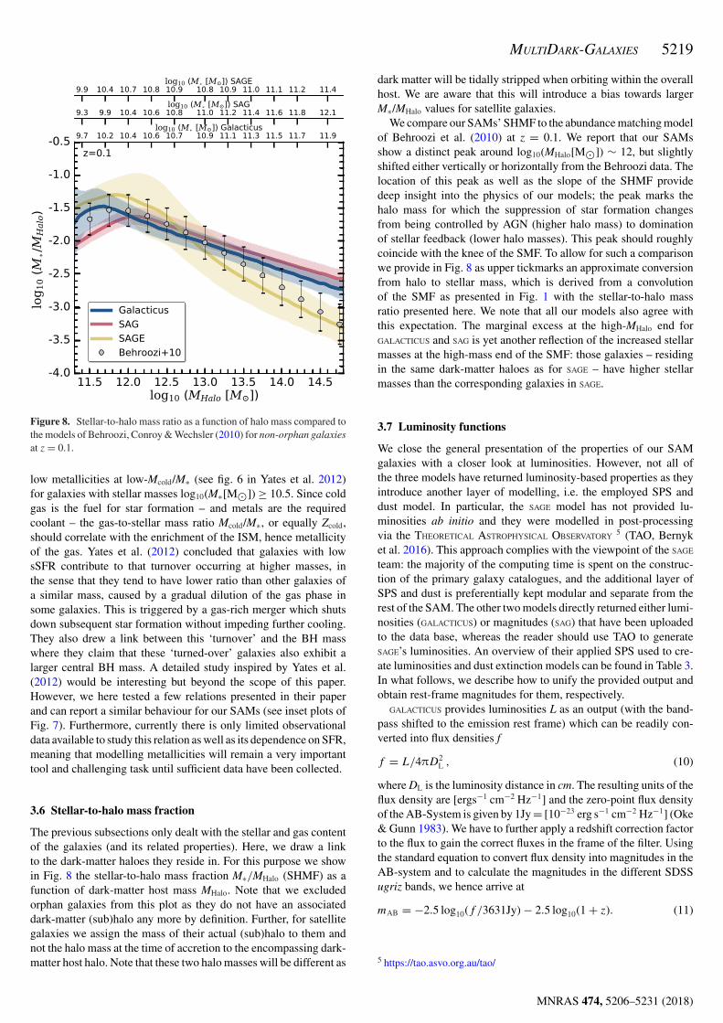
MULTIDARK-GALAXIES 5219

Figure 8. Stellar-to-halo mass ratio as a function of halo mass compared tothe models of Behroozi, Conroy & Wechsler (2010) for non-orphan galaxiesat z = 0.1.

low metallicities at low-Mcold/M∗ (see fig. 6 in Yates et al. 2012)for galaxies with stellar masses log10(M∗[M⊙]) ≥ 10.5. Since coldgas is the fuel for star formation – and metals are the requiredcoolant – the gas-to-stellar mass ratio Mcold/M∗, or equally Zcold,should correlate with the enrichment of the ISM, hence metallicityof the gas. Yates et al. (2012) concluded that galaxies with lowsSFR contribute to that turnover occurring at higher masses, inthe sense that they tend to have lower ratio than other galaxies ofa similar mass, caused by a gradual dilution of the gas phase insome galaxies. This is triggered by a gas-rich merger which shutsdown subsequent star formation without impeding further cooling.They also drew a link between this ‘turnover’ and the BH masswhere they claim that these ‘turned-over’ galaxies also exhibit alarger central BH mass. A detailed study inspired by Yates et al.(2012) would be interesting but beyond the scope of this paper.However, we here tested a few relations presented in their paperand can report a similar behaviour for our SAMs (see inset plots ofFig. 7). Furthermore, currently there is only limited observationaldata available to study this relation as well as its dependence on SFR,meaning that modelling metallicities will remain a very importanttool and challenging task until sufficient data have been collected.

3.6 Stellar-to-halo mass fraction

The previous subsections only dealt with the stellar and gas contentof the galaxies (and its related properties). Here, we draw a linkto the dark-matter haloes they reside in. For this purpose we showin Fig. 8 the stellar-to-halo mass fraction M∗/MHalo (SHMF) as afunction of dark-matter host mass MHalo. Note that we excludedorphan galaxies from this plot as they do not have an associateddark-matter (sub)halo any more by definition. Further, for satellitegalaxies we assign the mass of their actual (sub)halo to them andnot the halo mass at the time of accretion to the encompassing dark-matter host halo. Note that these two halo masses will be different as

dark matter will be tidally stripped when orbiting within the overallhost. We are aware that this will introduce a bias towards largerM∗/MHalo values for satellite galaxies.

We compare our SAMs’ SHMF to the abundance matching modelof Behroozi et al. (2010) at z = 0.1. We report that our SAMsshow a distinct peak around log10(MHalo[M⊙]) ∼ 12, but slightlyshifted either vertically or horizontally from the Behroozi data. Thelocation of this peak as well as the slope of the SHMF providedeep insight into the physics of our models; the peak marks thehalo mass for which the suppression of star formation changesfrom being controlled by AGN (higher halo mass) to dominationof stellar feedback (lower halo masses). This peak should roughlycoincide with the knee of the SMF. To allow for such a comparisonwe provide in Fig. 8 as upper tickmarks an approximate conversionfrom halo to stellar mass, which is derived from a convolutionof the SMF as presented in Fig. 1 with the stellar-to-halo massratio presented here. We note that all our models also agree withthis expectation. The marginal excess at the high-MHalo end forGALACTICUS and SAG is yet another reflection of the increased stellarmasses at the high-mass end of the SMF: those galaxies – residingin the same dark-matter haloes as for SAGE – have higher stellarmasses than the corresponding galaxies in SAGE.

3.7 Luminosity functions

We close the general presentation of the properties of our SAMgalaxies with a closer look at luminosities. However, not all ofthe three models have returned luminosity-based properties as theyintroduce another layer of modelling, i.e. the employed SPS anddust model. In particular, the SAGE model has not provided lu-minosities ab initio and they were modelled in post-processingvia the THEORETICAL ASTROPHYSICAL OBSERVATORY 5 (TAO, Bernyket al. 2016). This approach complies with the viewpoint of the SAGE

team: the majority of the computing time is spent on the construc-tion of the primary galaxy catalogues, and the additional layer ofSPS and dust is preferentially kept modular and separate from therest of the SAM. The other two models directly returned either lumi-nosities (GALACTICUS) or magnitudes (SAG) that have been uploadedto the data base, whereas the reader should use TAO to generateSAGE’s luminosities. An overview of their applied SPS used to cre-ate luminosities and dust extinction models can be found in Table 3.In what follows, we describe how to unify the provided output andobtain rest-frame magnitudes for them, respectively.

GALACTICUS provides luminosities L as an output (with the band-pass shifted to the emission rest frame) which can be readily con-verted into flux densities f

f = L/4πD2L , (10)

where DL is the luminosity distance in cm. The resulting units of theflux density are [ergs−1 cm−2 Hz−1] and the zero-point flux densityof the AB-System is given by 1Jy = [10−23 erg s−1 cm−2 Hz−1] (Oke& Gunn 1983). We have to further apply a redshift correction factorto the flux to gain the correct fluxes in the frame of the filter. Usingthe standard equation to convert flux density into magnitudes in theAB-system and to calculate the magnitudes in the different SDSSugriz bands, we hence arrive at

mAB = −2.5 log10(f /3631Jy) − 2.5 log10(1 + z). (11)

5 https://tao.asvo.org.au/tao/

MNRAS 474, 5206–5231 (2018)

Dow

nloaded from https://academ

ic.oup.com/m

nras/article-abstract/474/4/5206/4494373 by Konkoly Observatory user on 23 Septem

ber 2019

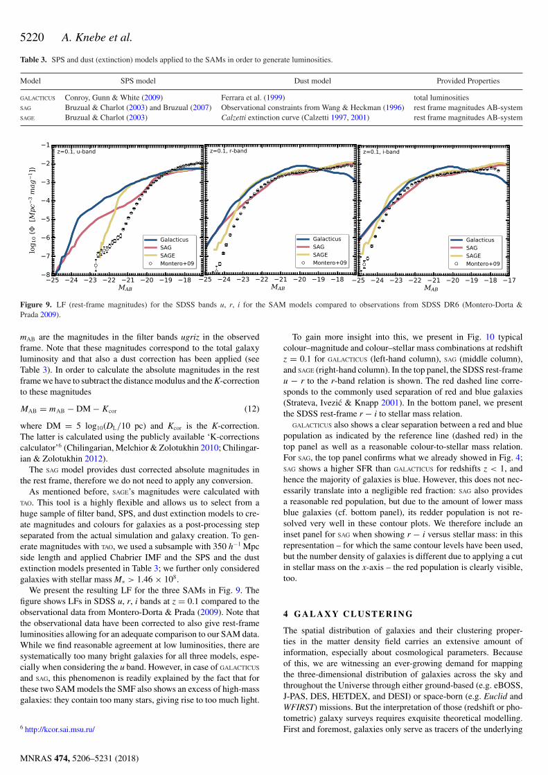
5220 A. Knebe et al.

Table 3. SPS and dust (extinction) models applied to the SAMs in order to generate luminosities.

Model SPS model Dust model Provided Properties

GALACTICUS Conroy, Gunn & White (2009) Ferrara et al. (1999) total luminositiesSAG Bruzual & Charlot (2003) and Bruzual (2007) Observational constraints from Wang & Heckman (1996) rest frame magnitudes AB-systemSAGE Bruzual & Charlot (2003) Calzetti extinction curve (Calzetti 1997, 2001) rest frame magnitudes AB-system

Figure 9. LF (rest-frame magnitudes) for the SDSS bands u, r, i for the SAM models compared to observations from SDSS DR6 (Montero-Dorta &Prada 2009).

mAB are the magnitudes in the filter bands ugriz in the observedframe. Note that these magnitudes correspond to the total galaxyluminosity and that also a dust correction has been applied (seeTable 3). In order to calculate the absolute magnitudes in the restframe we have to subtract the distance modulus and the K-correctionto these magnitudes

MAB = mAB − DM − Kcor (12)

where DM = 5 log10(DL/10 pc) and Kcor is the K-correction.The latter is calculated using the publicly available ‘K-correctionscalculator’6 (Chilingarian, Melchior & Zolotukhin 2010; Chilingar-ian & Zolotukhin 2012).

The SAG model provides dust corrected absolute magnitudes inthe rest frame, therefore we do not need to apply any conversion.

As mentioned before, SAGE’s magnitudes were calculated withTAO. This tool is a highly flexible and allows us to select from ahuge sample of filter band, SPS, and dust extinction models to cre-ate magnitudes and colours for galaxies as a post-processing stepseparated from the actual simulation and galaxy creation. To gen-erate magnitudes with TAO, we used a subsample with 350 h−1 Mpcside length and applied Chabrier IMF and the SPS and the dustextinction models presented in Table 3; we further only consideredgalaxies with stellar mass M∗ > 1.46 × 108.

We present the resulting LF for the three SAMs in Fig. 9. Thefigure shows LFs in SDSS u, r, i bands at z = 0.1 compared to theobservational data from Montero-Dorta & Prada (2009). Note thatthe observational data have been corrected to also give rest-frameluminosities allowing for an adequate comparison to our SAM data.While we find reasonable agreement at low luminosities, there aresystematically too many bright galaxies for all three models, espe-cially when considering the u band. However, in case of GALACTICUS

and SAG, this phenomenon is readily explained by the fact that forthese two SAM models the SMF also shows an excess of high-massgalaxies: they contain too many stars, giving rise to too much light.

6 http://kcor.sai.msu.ru/

To gain more insight into this, we present in Fig. 10 typicalcolour–magnitude and colour–stellar mass combinations at redshiftz = 0.1 for GALACTICUS (left-hand column), SAG (middle column),and SAGE (right-hand column). In the top panel, the SDSS rest-frameu − r to the r-band relation is shown. The red dashed line corre-sponds to the commonly used separation of red and blue galaxies(Strateva, Ivezic & Knapp 2001). In the bottom panel, we presentthe SDSS rest-frame r − i to stellar mass relation.

GALACTICUS also shows a clear separation between a red and bluepopulation as indicated by the reference line (dashed red) in thetop panel as well as a reasonable colour-to-stellar mass relation.For SAG, the top panel confirms what we already showed in Fig. 4;SAG shows a higher SFR than GALACTICUS for redshifts z < 1, andhence the majority of galaxies is blue. However, this does not nec-essarily translate into a negligible red fraction: SAG also providesa reasonable red population, but due to the amount of lower massblue galaxies (cf. bottom panel), its redder population is not re-solved very well in these contour plots. We therefore include aninset panel for SAG when showing r − i versus stellar mass: in thisrepresentation – for which the same contour levels have been used,but the number density of galaxies is different due to applying a cutin stellar mass on the x-axis – the red population is clearly visible,too.

4 G A L A X Y C L U S T E R I N G

The spatial distribution of galaxies and their clustering proper-ties in the matter density field carries an extensive amount ofinformation, especially about cosmological parameters. Becauseof this, we are witnessing an ever-growing demand for mappingthe three-dimensional distribution of galaxies across the sky andthroughout the Universe through either ground-based (e.g. eBOSS,J-PAS, DES, HETDEX, and DESI) or space-born (e.g. Euclid andWFIRST) missions. But the interpretation of those (redshift or pho-tometric) galaxy surveys requires exquisite theoretical modelling.First and foremost, galaxies only serve as tracers of the underlying

MNRAS 474, 5206–5231 (2018)

Dow

nloaded from https://academ

ic.oup.com/m

nras/article-abstract/474/4/5206/4494373 by Konkoly Observatory user on 23 Septem

ber 2019

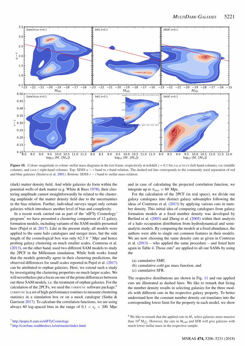
MULTIDARK-GALAXIES 5221

Figure 10. Colour–magnitude or colour–stellar mass diagrams in the rest frame, respectively at redshift z = 0.1 for GALACTICUS (left-hand column), SAG (middlecolumn), and SAGE ( right-hand column). Top: SDSS u − r band to r-band relation. The dashed red line corresponds to the commonly used separation of redand blue galaxies (Strateva et al. 2001). Bottom: SDSS r − i band to stellar mass relation.

(dark) matter density field. And while galaxies do form within thepotential wells of dark matter (e.g. White & Rees 1978), their clus-tering amplitude cannot straightforwardly be related to the cluster-ing amplitude of the matter density field due to the uncertaintiesin the bias relation. Further, individual surveys target only certaingalaxies which introduces another level of bias and complexity.

In a recent work carried out as part of the ‘nIFTy Cosmology’program7 we have presented a clustering comparison of 12 galaxyformation models, including variants of the SAM models presentedhere (Pujol et al. 2017). Like in the present study, all models wereapplied to the same halo catalogues and merger trees, but the sidelength of the cosmological box was only 62.5 h−1 Mpc and henceprobing galaxy clustering on much smaller scales. Contreras et al.(2013), on the other hand, used two different SAM models to studythe 2PCF in the Millenium simulation. While both works foundthat the models generally agree in their clustering predictions, theobserved differences for small scales reported in Pujol et al. (2017)can be attributed to orphan galaxies. Here, we extend such a studyby investigating the clustering properties on much larger scales. Wewill nevertheless put a focus on one of the prime differences betweenour three SAM models, i.e. the treatment of orphan galaxies. For thecalculation of the 2PCFs, we used the CORRFUNC software package.8

CORRFUNC is a set of high-performance routines to measure clusteringstatistics in a simulation box or on a mock catalogue (Sinha &Garrison 2017). To calculate the correlation functions, we are usingalways 60 log-spaced bins in the range of 0.1 < rp < 200 Mpc

7 http://popia.ft.uam.es/nIFTyCosmology8 http://corrfunc.readthedocs.io/en/master/index.html

and in case of calculating the projected correlation function, weintegrate up to πmax = 60 Mpc.

For the calculation of the 2PCF (in real space), we divide ourgalaxy catalogues into distinct galaxy subsamples following theideas of Contreras et al. (2013) by applying various cuts in num-ber density. This initial idea of comparing catalogues from galaxyformation models at a fixed number density was developed byBerlind et al. (2003) and Zheng et al. (2005) within their analysisof a halo occupation distribution from hydrodynamical and semi-analytic models. By comparing the models at a fixed abundance, theauthors were able to single out common features in their models.We are now choosing the same density cuts as given in Contreraset al. (2013) – who applied the same procedure – and listed hereagain in Table 4. Those cuts9 are applied to all our SAMs by usingthe

(a) cumulative SMF,(b) cumulative cold gas mass function, and(c) cumulative SFR.

The respective distributions are shown in Fig. 11 and our appliedcuts are illustrated as dashed lines. We like to remark that fixingthe number density results in selecting galaxies for the three mod-els with different cuts in the respective galaxy property. To betterunderstand how the constant number density cut translates into thecorresponding lower limit for the property in each model, we show

9 We like to remark that the applied cuts in M∗ select galaxies more massivethan 109 M⊙. However, the cuts in Mcold and SFR will give galaxies withmuch lower stellar mass in the respective sample.

MNRAS 474, 5206–5231 (2018)

Dow

nloaded from https://academ

ic.oup.com/m

nras/article-abstract/474/4/5206/4494373 by Konkoly Observatory user on 23 Septem

ber 2019

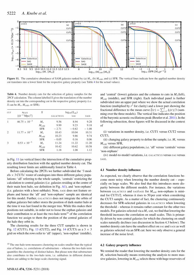
5222 A. Knebe et al.

Figure 11. The cumulative abundance of SAM galaxies ranked by (a) M∗, (b) Mcold, and (c) SFR. The vertical lines indicate how the applied number densitycut translates into a lower limit for the respective galaxy property (see Table 4 for the actual values).

Table 4. Number density cuts for the selection of galaxy samples for the2PCF calculation. The column labelled X gives the translation of the numberdensity cut into the corresponding cut in the respective galaxy property (i.e.X can be M∗, Mcold, or SFR).

CUT nCUT X log10(Xcut)[(h−1 Mpc)3] GALACTICUS SAG SAGE

1 46.75 × 10−3 M∗ 9.56 8.94 9.28Mcold 9.99 9.23 9.18SFR − 2.71 − 0.82 − 1.08

2 11.77 × 10−3 M∗ 10.43 10.04 10.31Mcold 10.23 9.86 9.74SFR − 0.05 0.16 0.06

3 0.53 × 10−3 M∗ 11.24 11.22 11.20Mcold 10.42 10.62 10.58SFR 1.18 1.08 1.12

in Fig. 11 (as vertical lines) the intersection of the cumulative prop-erty distribution function with the applied number density cut. Theresulting lower limits are additionally listed in Table 4.

Before calculating the 2PCFs we further subdivided the ‘3 mod-els × 3 CUTs’ roster of catalogues into three different galaxy popu-lations: ‘all’ referring to the whole sample, ‘centrals’ restricting thecalculation to central galaxies (i.e. galaxies residing at the centre oftheir main host halo, see definition in Fig. A1), and ‘non-orphans’(i.e. galaxies with a host subhalo). Note, SAGE does not feature or-phans and hence the ‘all’ and ‘non-orphans’ sample are identicalfor this model. Further, GALACTICUS does not integrate the orbits oforphan galaxies but rather stores the position of dark-matter halo atthe time it was last found in the merger tree. While this makes theirpositions not suitable, in order not to loose the orphan galaxies andtheir contribution to at least the two-halo term10 of the correlationfunction we assign to them the position of the central galaxies ofthe halo they orbit in.

The clustering results for the three CUT samples is shown inFig. 12 (CUT1), Fig. 13 (CUT2), and Fig. 14 (CUT3) as a 3 × 3grid on which the rows refer to ‘all’ (upper), ‘non-orphan’ (middle),

10 The one-halo term measures clustering on scales smaller than the typicalsize of haloes, i.e. correlations of substructure – whereas the two-halo termquantifies the clustering of distinct haloes. But please note that substructurealso contributes to the two-halo term, i.e. subhaloes in different distincthaloes are adding to the large-scale clustering signal.

and ‘central’ (lower) galaxies and the columns to cuts in M∗(left),Mcold (middle), and SFR (right). Each individual panel is furthersubdivided into an upper part where we show the actual correlationfunction (multiplied by r2 for clarity) and a lower part showing thefractional difference to the mean curve ξ (r) =

&3i=1 ξi(r)/3 (sum-

ming over the three models). The vertical line indicates the positionof the baryonic acoustic oscillations peak (Beutler et al. 2011). In thefollowing subsection, those figures will be discussed in the contextof

(i) variations in number density, i.e. CUT1 versus CUT2 versusCUT3,

(ii) changing galaxy property to define the sample, i.e. M∗ versusMcold versus SFR,

(iii) different galaxy populations, i.e. ‘all’ versus ‘centrals’ versus‘non-orphans’

(iv) model-to-model variations, i.e. GALACTICUS versus SAG versusSAGE.

4.1 Number density influence

As expected, we clearly observe that the correlation functions be-come more noisy when lowering the number density cut – espe-cially on large scales. We also find that this introduces more dis-parity between the different models. For instance, the variationsbetween GALACTICUS and SAG/SAGE for Mcold non-orphans is mini-mal for CUT1/2, whereas it rises to 50 per cent when consideringthe CUT3 sample. As a matter of fact, the clustering continuouslydecreases for SFR-selected galaxies in GALACTICUS when loweringthe threshold – whereas it remains rather constant for the other twomodels. For galaxies selected via a M∗-cut, we find that lowering thethreshold increases the correlation on small scales. This is primar-ily driven by non-central galaxies for which the clustering on smallscales naturally declines (see discussion in Section 4.3 below). Thenumber density cuts have the smallest effect on SAG and SAGE as wellas galaxies selected via an SFR cut: here we only observe a generalincrease of the noise level.

4.2 Galaxy property influence

We remind the reader that lowering the number density cuts for theM∗ selection basically means restricting the analysis to more mas-sive galaxies, lowering in Mcold selects those with huge reservoirs of

MNRAS 474, 5206–5231 (2018)

Dow

nloaded from https://academ

ic.oup.com/m

nras/article-abstract/474/4/5206/4494373 by Konkoly Observatory user on 23 Septem

ber 2019

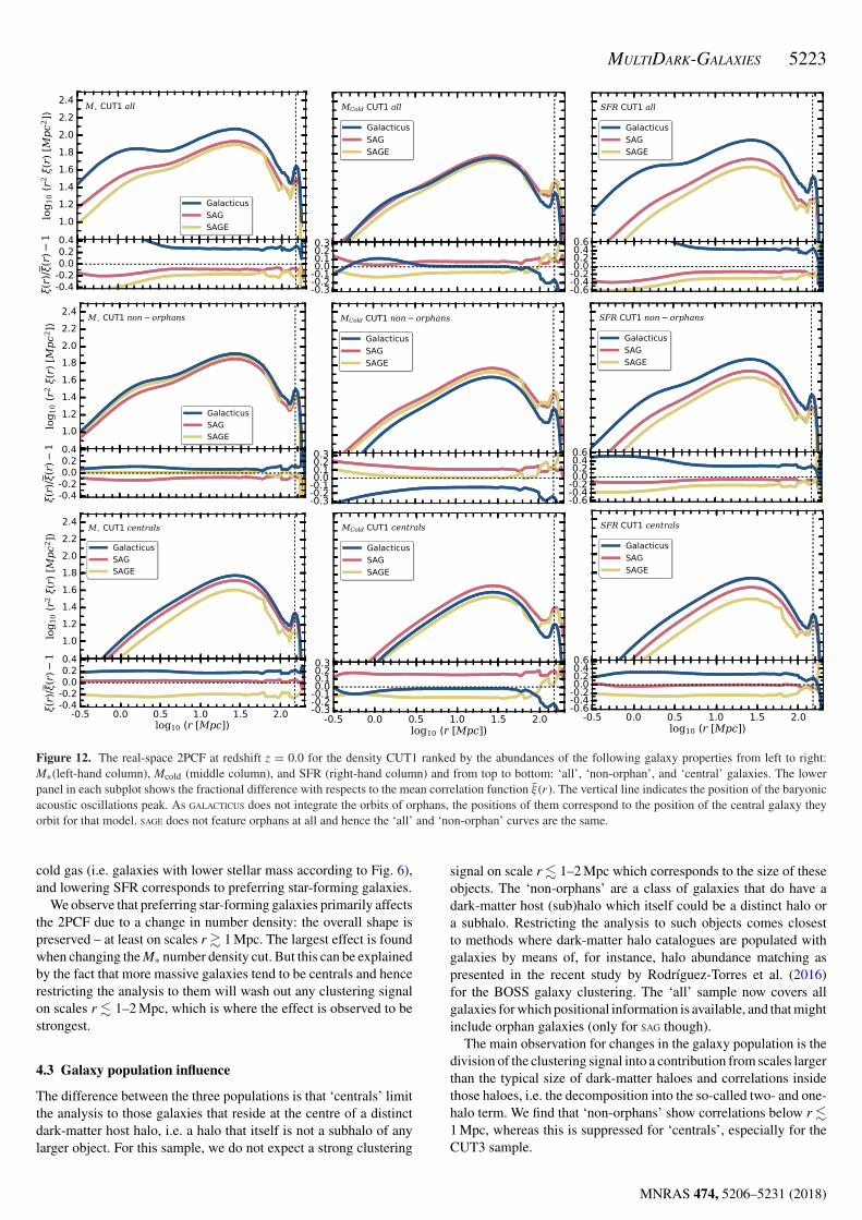
MULTIDARK-GALAXIES 5223

Figure 12. The real-space 2PCF at redshift z = 0.0 for the density CUT1 ranked by the abundances of the following galaxy properties from left to right:M∗(left-hand column), Mcold (middle column), and SFR (right-hand column) and from top to bottom: ‘all’, ‘non-orphan’, and ‘central’ galaxies. The lowerpanel in each subplot shows the fractional difference with respects to the mean correlation function ξ (r). The vertical line indicates the position of the baryonicacoustic oscillations peak. As GALACTICUS does not integrate the orbits of orphans, the positions of them correspond to the position of the central galaxy theyorbit for that model. SAGE does not feature orphans at all and hence the ‘all’ and ‘non-orphan’ curves are the same.

cold gas (i.e. galaxies with lower stellar mass according to Fig. 6),and lowering SFR corresponds to preferring star-forming galaxies.

We observe that preferring star-forming galaxies primarily affectsthe 2PCF due to a change in number density: the overall shape ispreserved – at least on scales r ! 1 Mpc. The largest effect is foundwhen changing the M∗ number density cut. But this can be explainedby the fact that more massive galaxies tend to be centrals and hencerestricting the analysis to them will wash out any clustering signalon scales r " 1–2 Mpc, which is where the effect is observed to bestrongest.

4.3 Galaxy population influence

The difference between the three populations is that ‘centrals’ limitthe analysis to those galaxies that reside at the centre of a distinctdark-matter host halo, i.e. a halo that itself is not a subhalo of anylarger object. For this sample, we do not expect a strong clustering

signal on scale r " 1–2 Mpc which corresponds to the size of theseobjects. The ‘non-orphans’ are a class of galaxies that do have adark-matter host (sub)halo which itself could be a distinct halo ora subhalo. Restricting the analysis to such objects comes closestto methods where dark-matter halo catalogues are populated withgalaxies by means of, for instance, halo abundance matching aspresented in the recent study by Rodrıguez-Torres et al. (2016)for the BOSS galaxy clustering. The ‘all’ sample now covers allgalaxies for which positional information is available, and that mightinclude orphan galaxies (only for SAG though).

The main observation for changes in the galaxy population is thedivision of the clustering signal into a contribution from scales largerthan the typical size of dark-matter haloes and correlations insidethose haloes, i.e. the decomposition into the so-called two- and one-halo term. We find that ‘non-orphans’ show correlations below r "1 Mpc, whereas this is suppressed for ‘centrals’, especially for theCUT3 sample.

MNRAS 474, 5206–5231 (2018)

Dow

nloaded from https://academ

ic.oup.com/m

nras/article-abstract/474/4/5206/4494373 by Konkoly Observatory user on 23 Septem

ber 2019

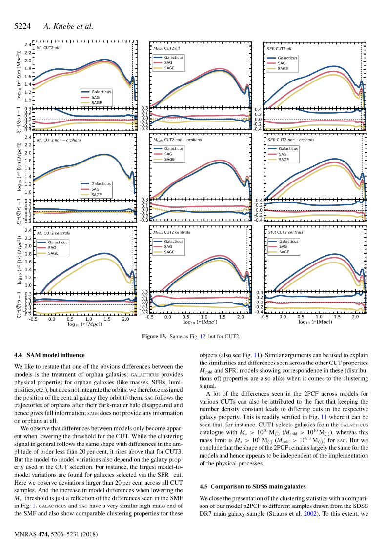
5224 A. Knebe et al.

Figure 13. Same as Fig. 12, but for CUT2.

4.4 SAM model influence

We like to restate that one of the obvious differences between themodels is the treatment of orphan galaxies: GALACTICUS providesphysical properties for orphan galaxies (like masses, SFRs, lumi-nosities, etc.), but does not integrate the orbits; we therefore assignedthe position of the central galaxy they orbit to them. SAG follows thetrajectories of orphans after their dark-matter halo disappeared andhence gives full information; SAGE does not provide any informationon orphans at all.

We observe that differences between models only become appar-ent when lowering the threshold for the CUT. While the clusteringsignal in general follows the same shape with differences in the am-plitude of order less than 20 per cent, it rises above that for CUT3.But the model-to-model variations also depend on the galaxy prop-erty used in the CUT selection. For instance, the largest model-to-model variations are found for galaxies selected via the SFR cut.Here we observe deviations larger than 20 per cent across all CUTsamples. And the increase in model differences when lowering theM∗ threshold is just a reflection of the differences seen in the SMFin Fig. 1. GALACTICUS and SAG have a very similar high-mass end ofthe SMF and also show comparable clustering properties for these

objects (also see Fig. 11). Similar arguments can be used to explainthe similarities and differences seen across the other CUT propertiesMcold and SFR: models showing correspondence in these (distribu-tions of) properties are also alike when it comes to the clusteringsignal.

A lot of the differences seen in the 2PCF across models forvarious CUTs can also be attributed to the fact that keeping thenumber density constant leads to differing cuts in the respectivegalaxy property. This is readily verified in Fig. 11 where it can beseen that, for instance, CUT1 selects galaxies from the GALACTICUS

catalogue with M∗ > 1010 M⊙ (Mcold > 1010 M⊙), whereas thismass limit is M∗ > 109 M⊙ (Mcold > 109.3 M⊙) for SAG. But weconclude that the shape of the 2PCF remains largely the same for themodels and hence appears to be independent of the implementationof the physical processes.

4.5 Comparison to SDSS main galaxies

We close the presentation of the clustering statistics with a compari-son of our model p2PCF to different samples drawn from the SDSSDR7 main galaxy sample (Strauss et al. 2002). To this extent, we

MNRAS 474, 5206–5231 (2018)

Dow

nloaded from https://academ

ic.oup.com/m

nras/article-abstract/474/4/5206/4494373 by Konkoly Observatory user on 23 Septem

ber 2019

MULTIDARK-GALAXIES 5225

Figure 14. Same as Fig. 12, but for CUT3.

selected SAM galaxy samples within the following four absoluter-band magnitude bins

(a) Mr ∈ [−19, −18],(b) Mr ∈ [−20, −19],(c) Mr ∈ [−21, −20], and(d) Mr ∈ [−22, −21].

Note that the samples are only selected by r-band magnitude andno additional cuts have been made.

As for the real-space correlation function, we used the CORRFUNC

PYTHON package and compute the projected correlation function bychoosing an integration length of πmax = 60 Mpc. We also tested ifa different integration length would change our results, but cannotreport any relevant differences when using πmax = [40, 80, 100]Mpc.

Our results can be viewed in Fig. 15 where show the p2PCF forthe aforementioned four magnitude bins. In each of the panels, wefurther compare them to the SDSS results from Zehavi et al. (2011,table 7) at z ∼ 0.1, within the same magnitude bins. The upper part ofeach panel shows the correlation function with the observations asopen circles and the lower part represents the residuals with respect

to the observations in the respective magnitude bin. In Table 5, weshow the number densities and the fraction of satellites and orphansatellites, respectively, of our samples presented in Fig. 15.

All our models reproduce the basic features of the observationalp2PCF, and the transition from the one- to the two-halo term ataround rp ∼1–2 Mpc is well described. Especially in the bin (a)where SAG and SAGE reproduce the SDSS clustering signal perfectlyfor large separations, and in (b) where GALACTICUS describes theobservational data best, and within 15 per cent–40 per cent. Thiscan be understood if we take a look at the fraction of satellites inTable 5. GALACTICUS shows the largest fraction of satellites – whencombining satellites and orphans together – and the largest frac-tion of orphans, respectively. As we discussed in previous sections,this again confirms how strong the clustering behaviour correlateswith the galaxy type (see Figs 12–14): models (in our case SAG

and SAGE) with smaller satellite fraction lack clustering power onsmall scales, but nevertheless reproduce the observed p2PCF verywell beyond the one-halo term. However, we also need to remindthe reader that the positions for the orphans in GALACTICUS coincidewith the position of the central galaxy as that model does not inte-grate the orbits of satellite galaxies once they are stripped off their

MNRAS 474, 5206–5231 (2018)

Dow

nloaded from https://academ

ic.oup.com/m

nras/article-abstract/474/4/5206/4494373 by Konkoly Observatory user on 23 Septem

ber 2019

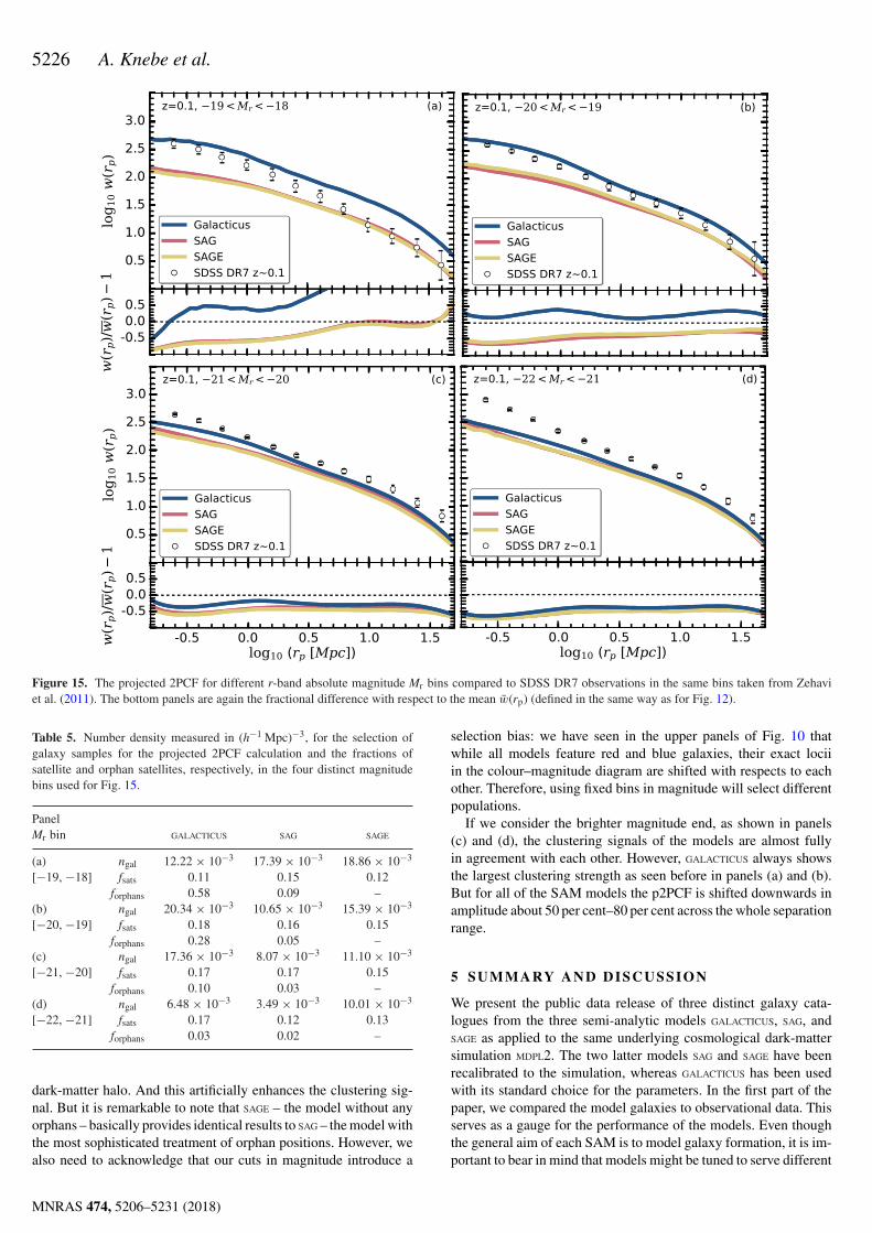
5226 A. Knebe et al.

Figure 15. The projected 2PCF for different r-band absolute magnitude Mr bins compared to SDSS DR7 observations in the same bins taken from Zehaviet al. (2011). The bottom panels are again the fractional difference with respect to the mean w(rp) (defined in the same way as for Fig. 12).

Table 5. Number density measured in (h−1 Mpc)−3, for the selection ofgalaxy samples for the projected 2PCF calculation and the fractions ofsatellite and orphan satellites, respectively, in the four distinct magnitudebins used for Fig. 15.

PanelMr bin GALACTICUS SAG SAGE

(a) ngal 12.22 × 10−3 17.39 × 10−3 18.86 × 10−3

[−19, −18] fsats 0.11 0.15 0.12forphans 0.58 0.09 –

(b) ngal 20.34 × 10−3 10.65 × 10−3 15.39 × 10−3

[−20, −19] fsats 0.18 0.16 0.15forphans 0.28 0.05 –

(c) ngal 17.36 × 10−3 8.07 × 10−3 11.10 × 10−3

[−21, −20] fsats 0.17 0.17 0.15forphans 0.10 0.03 –

(d) ngal 6.48 × 10−3 3.49 × 10−3 10.01 × 10−3

[−22, −21] fsats 0.17 0.12 0.13forphans 0.03 0.02 –

dark-matter halo. And this artificially enhances the clustering sig-nal. But it is remarkable to note that SAGE – the model without anyorphans – basically provides identical results to SAG – the model withthe most sophisticated treatment of orphan positions. However, wealso need to acknowledge that our cuts in magnitude introduce a

selection bias: we have seen in the upper panels of Fig. 10 thatwhile all models feature red and blue galaxies, their exact lociiin the colour–magnitude diagram are shifted with respects to eachother. Therefore, using fixed bins in magnitude will select differentpopulations.

If we consider the brighter magnitude end, as shown in panels(c) and (d), the clustering signals of the models are almost fullyin agreement with each other. However, GALACTICUS always showsthe largest clustering strength as seen before in panels (a) and (b).But for all of the SAM models the p2PCF is shifted downwards inamplitude about 50 per cent–80 per cent across the whole separationrange.

5 SU M M A RY A N D D I S C U S S I O N

We present the public data release of three distinct galaxy cata-logues from the three semi-analytic models GALACTICUS, SAG, andSAGE as applied to the same underlying cosmological dark-mattersimulation MDPL2. The two latter models SAG and SAGE have beenrecalibrated to the simulation, whereas GALACTICUS has been usedwith its standard choice for the parameters. In the first part of thepaper, we compared the model galaxies to observational data. Thisserves as a gauge for the performance of the models. Even thoughthe general aim of each SAM is to model galaxy formation, it is im-portant to bear in mind that models might be tuned to serve different

MNRAS 474, 5206–5231 (2018)

Dow

nloaded from https://academ

ic.oup.com/m

nras/article-abstract/474/4/5206/4494373 by Konkoly Observatory user on 23 Septem

ber 2019

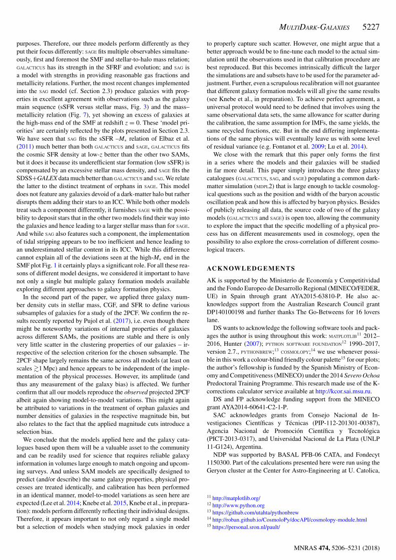
MULTIDARK-GALAXIES 5227

purposes. Therefore, our three models perform differently as theyput their focus differently: SAGE fits multiple observables simultane-ously, first and foremost the SMF and stellar-to-halo mass relation;GALACTICUS has its strength in the SFRF and evolution; and SAG isa model with strengths in providing reasonable gas fractions andmetallicity relations. Further, the most recent changes implementedinto the SAG model (cf. Section 2.3) produce galaxies with prop-erties in excellent agreement with observations such as the galaxymain sequence (sSFR versus stellar mass, Fig. 3) and the mass–metallicity relation (Fig. 7), yet showing an excess of galaxies atthe high-mass end of the SMF at redshift z = 0. These ‘model pri-orities’ are certainly reflected by the plots presented in Section 2.3.We have seen that SAG fits the sSFR –M∗ relation of Elbaz et al.(2011) much better than both GALACTICUS and SAGE, GALACTICUS fitsthe cosmic SFR density at low-z better than the other two SAMs,but it does it because its underefficient star formation (low sSFR) iscompensated by an excessive stellar mass density, and SAGE fits theSDSS+GALEX data much better than GALACTICUS and SAG. We relatethe latter to the distinct treatment of orphans in SAGE. This modeldoes not feature any galaxies devoid of a dark-matter halo but ratherdisrupts them adding their stars to an ICC. While both other modelstreat such a component differently, it furnishes SAGE with the possi-bility to deposit stars that in the other two models find their way intothe galaxies and hence leading to a larger stellar mass than for SAGE.And while SAG also features such a component, the implementationof tidal stripping appears to be too inefficient and hence leading toan underestimated stellar content in its ICC. While this differencecannot explain all of the deviations seen at the high-M∗ end in theSMF plot Fig. 1 it certainly plays a significant role. For all these rea-sons of different model designs, we considered it important to havenot only a single but multiple galaxy formation models availableexploring different approaches to galaxy formation physics.

In the second part of the paper, we applied three galaxy num-ber density cuts in stellar mass, CGF, and SFR to define varioussubsamples of galaxies for a study of the 2PCF. We confirm the re-sults recently reported by Pujol et al. (2017), i.e. even though theremight be noteworthy variations of internal properties of galaxiesacross different SAMs, the positions are stable and there is onlyvery little scatter in the clustering properties of our galaxies – ir-respective of the selection criterion for the chosen subsample. The2PCF shape largely remains the same across all models (at least onscales !1 Mpc) and hence appears to be independent of the imple-mentation of the physical processes. However, its amplitude (andthus any measurement of the galaxy bias) is affected. We furtherconfirm that all our models reproduce the observed projected 2PCFalbeit again showing model-to-model variations. This might againbe attributed to variations in the treatment of orphan galaxies andnumber densities of galaxies in the respective magnitude bin, butalso relates to the fact that the applied magnitude cuts introduce aselection bias.

We conclude that the models applied here and the galaxy cata-logues based upon them will be a valuable asset to the communityand can be readily used for science that requires reliable galaxyinformation in volumes large enough to match ongoing and upcom-ing surveys. And unless SAM models are specifically designed topredict (and/or describe) the same galaxy properties, physical pro-cesses are treated identically, and calibration has been performedin an identical manner, model-to-model variations as seen here areexpected (Lee et al. 2014; Knebe et al. 2015, Knebe et al., in prepara-tion): models perform differently reflecting their individual designs.Therefore, it appears important to not only regard a single modelbut a selection of models when studying mock galaxies in order

to properly capture such scatter. However, one might argue that abetter approach would be to fine-tune each model to the actual sim-ulation until the observations used in that calibration procedure arebest reproduced. But this becomes intrinsically difficult the largerthe simulations are and subsets have to be used for the parameter ad-justment. Further, even a scrupulous recalibration will not guaranteethat different galaxy formation models will all give the same results(see Knebe et al., in preparation). To achieve perfect agreement, auniversal protocol would need to be defined that involves using thesame observational data sets, the same allowance for scatter duringthe calibration, the same assumption for IMFs, the same yields, thesame recycled fractions, etc. But in the end differing implementa-tions of the same physics will eventually leave us with some levelof residual variance (e.g. Fontanot et al. 2009; Lu et al. 2014).

We close with the remark that this paper only forms the firstin a series where the models and their galaxies will be studiedin far more detail. This paper simply introduces the three galaxycatalogues (GALACTICUS, SAG, and SAGE) populating a common dark-matter simulation (MDPL2) that is large enough to tackle cosmolog-ical questions such as the position and width of the baryon acousticoscillation peak and how this is affected by baryon physics. Besidesof publicly releasing all data, the source code of two of the galaxymodels (GALACTICUS and SAGE) is open too, allowing the communityto explore the impact that the specific modelling of a physical pro-cess has on different measurements used in cosmology, open thepossibility to also explore the cross-correlation of different cosmo-logical tracers.

ACK NOW L E D G E M E N T S

AK is supported by the Ministerio de Economıa y Competitividadand the Fondo Europeo de Desarrollo Regional (MINECO/FEDER,UE) in Spain through grant AYA2015-63810-P. He also ac-knowledges support from the Australian Research Council grantDP140100198 and further thanks The Go-Betweens for 16 loverslane.

DS wants to acknowledge the following software tools and pack-ages the author is using throughout this work: MATPLOTLIB11 2012–2016, Hunter (2007); PYTHON SOFTWARE FOUNDATION12 1990–2017,version 2.7., PYTHONBREW;13 COSMOLOPY;14 we use whenever possi-ble in this work a colour-blind friendly colour palette15 for our plots;the author’s fellowship is funded by the Spanish Ministry of Econ-omy and Competitiveness (MINECO) under the 2014 Severo OchoaPredoctoral Training Programme. This research made use of the K-corrections calculator service available at http://kcor.sai.msu.ru.

DS and FP acknowledge funding support from the MINECOgrant AYA2014-60641-C2-1-P.

SAC acknowledges grants from Consejo Nacional de In-vestigaciones Cientıficas y Tecnicas (PIP-112-201301-00387),Agencia Nacional de Promocion Cientıfica y Tecnologica(PICT-2013-0317), and Universidad Nacional de La Plata (UNLP11-G124), Argentina.

NDP was supported by BASAL PFB-06 CATA, and Fondecyt1150300. Part of the calculations presented here were run using theGeryon cluster at the Center for Astro-Engineering at U. Catolica,

11 http://matplotlib.org/12 http://www.python.org13 https://github.com/utahta/pythonbrew14 http://roban.github.io/CosmoloPy/docAPI/cosmolopy-module.html15 https://personal.sron.nl/pault/

MNRAS 474, 5206–5231 (2018)

Dow

nloaded from https://academ

ic.oup.com/m

nras/article-abstract/474/4/5206/4494373 by Konkoly Observatory user on 23 Septem

ber 2019

5228 A. Knebe et al.

which received funding from QUIMAL 130008 and FondequipAIC-57.

CVM was supported by a fellowship from CONICET, Argentina.PB was supported by program number HST-HF2-51353.001-A,

provided by NASA through a Hubble Fellowship grant from theSpace Telescope Science Institute, which is operated by the As-sociation of Universities for Research in Astronomy, Incorporated,under NASA contract NAS5-26555.

VGP acknowledges support from the University of Portsmouththrough the Dennis Sciama Fellowship award.

GY is supported by the MINECO/FEDER, UE in Spain throughgrant AYA2015-63810-P.

We all thank the anonymous referee whose suggestions and re-marks greatly helped to improve the paper.

The COSMOSIM data base16 used in this paper is a service by theLeibniz-Institute for Astrophysics Potsdam. The MULTIDARK database was developed in cooperation with the Spanish MULTIDARK

Consolider Project CSD2009-00064.The SAGE galaxy model is a publicly available code base and

is available for download at https://github.com/darrencroton/sage.Magnitudes for SAGE galaxies were generated using Swinburne Uni-versity’s Theoretical Astrophysical Observatory (TAO). TAO is partof the Australian All-Sky Virtual Observatory and is freely acces-sible at https://tao.asvo.org.au.

The authors gratefully acknowledge the Gauss Centre for Su-percomputing e.V. (www.gauss-centre.eu) and the Partnership forAdvanced Supercomputing in Europe (www.prace-ri.eu) for fund-ing the MULTIDARK simulation project by providing computing timeon the GCS Supercomputer SuperMUC at Leibniz Supercomput-ing Centre (www.lrz.de). The MDPL2 simulation has been performedunder grant pr87yi.

The authors contributed to this paper in the following ways:AK and FP initiated and coordinated the project. DS created allthe plots. The three of them wrote the paper (with help from theremaining authors). GY (together with SG and AAK) ran the MDPL2simulation. SG, HE, NIL, and MSt provided access to the data baseto which KR uploaded the simulation, halo catalogues, merger trees,and eventually galaxy catalogues. PB generated the halo cataloguesand merger trees. CB and AB ran the GALACTICUS model over thesimulation. SAC, NDP, CAVM, and ANR ran the SAG model over thesimulation. DJC, ARHS, and MSi ran the SAGE model. All authorsproofread and commented on the paper.

This research has made use of NASA’s Astrophysics Data Systemand the arXiv preprint server.

R E F E R E N C E S

Allende Prieto C., Lambert D. L., Asplund M., 2001, ApJ, 556, L63Asplund M., Grevesse N., Sauval A. J., Scott P., 2009, ARA&A, 47, 481Avila S. et al., 2014, MNRAS, 441, 3488Baldry I. K., Glazebrook K., Driver S. P., 2008, MNRAS, 388, 945Baugh C. M., 2006, Rep. Prog. Phys., 69, 3101Begelman M. C., 2014, preprint (arXiv:1410.8132)Behroozi P. S., Conroy C., Wechsler R. H., 2010, ApJ, 717, 379Behroozi P. S., Wechsler R. H., Conroy C., 2013, ApJ, 770, 57Behroozi P. S., Wechsler R. H., Wu H.-Y., 2013a, ApJ, 762, 109Behroozi P. S., Wechsler R. H., Wu H.-Y., Busha M. T., Klypin A. A.,

Primack J. R., 2013b, ApJ, 763, 18Behroozi P. et al., 2015, MNRAS, 454, 3020Benson A. J., 2010, Phys. Rep., 495, 33Benson A. J., 2012, New Astron., 17, 175Benson A. J., Babul A., 2009, MNRAS, 397, 1302

16 http://www.cosmosim.org

Benson A. J., Bower R., 2011, MNRAS, 410, 2653Benson A. J., Cole S., Frenk C. S., Baugh C. M., Lacey C. G., 2000, MNRAS,

311, 793Benson A. J., Borgani S., De Lucia G., Boylan-Kolchin M., Monaco P.,

2012, MNRAS, 419, 3590Berlind A. A. et al., 2003, ApJ, 593, 1Bernyk M. et al., 2016, ApJS, 223, 9Bertschinger E., 1989, ApJ, 340, 666Beutler F. et al., 2011, MNRAS, 416, 3017Binney J., Tremaine S., 1987, Galactic Dynamics. Princeton Univ. Press,

Princeton, NJ, p. 747Boselli A., Cortese L., Boquien M., Boissier S., Catinella B., Lagos C.,

Saintonge A., 2014, A&A, 564, A66Bower R. G., Benson A. J., Malbon R., Helly J. C., Frenk C. S., Baugh C.

M., Cole S., Lacey C. G., 2006, MNRAS, 370, 645Boylan-Kolchin M., Ma C.-P., Quataert E., 2008, MNRAS, 383, 93Bruzual G., Charlot S., 2003, MNRAS, 344, 1000Bruzual G., 2007, in Vallenari A., Tantalo R., Portinari L., Moretti A., eds,

ASP Conf. Ser. Vol. 374, From Stars to Galaxies: Building the Pieces toBuild Upon the Universe. Astron. Soc. Pac., San Francisco, p. 303.

Bryan G. L., Norman M. L., 1998, ApJ, 495, 80Calzetti D., 1997, in Waller W. H., ed., AIP Conf. Ser., Vol. 408, The

Ultraviolet Universe at Low and High Redshift. AIP, Melville, NY,p. 403

Calzetti D., 2001, PASP, 113, 1449Chabrier G., 2003, PASP, 115, 763Chilingarian I. V., Zolotukhin I. Y., 2012, MNRAS, 419, 1727Chilingarian I. V., Melchior A.-L., Zolotukhin I. Y., 2010, MNRAS, 405,

1409Cole S. et al., 2001, MNRAS, 326, 255Comparat J., Prada F., Yepes G., Klypin A., 2017, MNRAS, 469, 4157Conroy C., Gunn J. E., White M., 2009, ApJ, 699, 486Contreras C. et al., 2013, MNRAS, 430, 924Cora S. A., 2006, MNRAS, 368, 1540Cowie L. L., Songaila A., Hu E. M., Cohen J. G., 1996, AJ, 112, 839Croton D. J. et al., 2006, MNRAS, 365, 11Croton D. J. et al., 2016, ApJS, 222, 22de Jong R. S., Lacey C., 2000, ApJ, 545, 781De Lucia G., Kauffmann G., White S. D. M., 2004, MNRAS, 349, 1101Diemer B., More S., Kravtsov A. V., 2013, ApJ, 766, 25Dolag K., 2015, IAU General Assembly, 22, 2250156Dubois Y. et al., 2014, MNRAS, 444, 1453Efstathiou G., Lake G., Negroponte J., 1982, MNRAS, 199, 1069Elbaz D. et al., 2011, A&A, 533, A119Ellison S. L., Patton D. R., Simard L., McConnachie A. W., 2008, AJ, 135,

1877Favole G. et al., 2016, MNRAS, 461, 3421Favole G., Rodrıguez-Torres S. A., Comparat J., Prada F., Guo H., Klypin

A., Montero-Dorta A. D., 2017, MNRAS, 472, 550Ferland G. J. et al., 2013, Rev. Mex. Astron. Astrofis., 49, 137Ferrara A., Bianchi S., Cimatti A., Giovanardi C., 1999, ApJS, 123,

437Fontanot F., De Lucia G., Monaco P., Somerville R. S., Santini P., 2009,

MNRAS, 397, 1776Foster A. R., Ji L., Smith R. K., Brickhouse N. S., 2012, ApJ, 756, 128Franx M., van Dokkum P. G., Forster Schreiber N. M., Wuyts S., Labbe I.,

Toft S., 2008, ApJ, 688, 770Gargiulo I. D. et al., 2015, MNRAS, 446, 3820Gnedin O. Y., Kravtsov A. V., Klypin A. A., Nagai D., 2004, ApJ, 616,

16Gonzalez-Perez V., Lacey C. G., Baugh C. M., Lagos C. D. P., Helly J.,

Campbell D. J. R., Mitchell P. D., 2014, MNRAS, 439, 264Gottlober S., Hoffman Y., Yepes G., 2010, in Wagner S., Steinmetz M.,

Bode A., Muller M. M., eds, High Performance Computing in Scienceand Engineering, Springer, Berlin, pp. 309–323.

Governato F. et al., 2010, Nature, 463, 203Grand R. J. J. et al., 2017, MNRAS, 467, 179Gruppioni C. et al., 2015, MNRAS, 451, 3419Guedes J., Callegari S., Madau P., Mayer L., 2011, ApJ, 742, 76

MNRAS 474, 5206–5231 (2018)

Dow

nloaded from https://academ

ic.oup.com/m

nras/article-abstract/474/4/5206/4494373 by Konkoly Observatory user on 23 Septem

ber 2019

MULTIDARK-GALAXIES 5229

Gunn J. E., Gott J. R. I., 1972, ApJ, 176, 1Guo Q. et al., 2011, MNRAS, 413, 101Guo Q., White S., Angulo R. E., Henriques B., Lemson G., Boylan-Kolchin

M., Thomas P., Short C., 2013, MNRAS, 428, 1351Guo Q. et al., 2016, MNRAS, 461, 3457Haring N., Rix H.-W., 2004, ApJ, 604, L89Henriques B. M. B., Thomas P. A., Oliver S., Roseboom I., 2009, MNRAS,

396, 535Henriques B. M. B., White S. D. M., Thomas P. A., Angulo R. E., Guo Q.,

Lemson G., Springel V., 2013, MNRAS, 431, 3373Henriques B. M. B., White S. D. M., Thomas P. A., Angulo R., Guo Q.,

Lemson G., Springel V., Overzier R., 2015, MNRAS, 451, 2663Hirschi R., Meynet G., Maeder A., 2005, A&A, 433, 1013Hirschmann M., De Lucia G., Fontanot F., 2016, MNRAS, 461, 1760Hopkins A. M., 2004, ApJ, 615, 209Hopkins P. F., Keres D., Onorbe J., Faucher-Giguere C.-A., Quataert E.,

Murray N., Bullock J. S., 2014, MNRAS, 445, 581Hunter J. D., 2007, Comput. Sci. Eng., 9, 90Iwamoto K., Brachwitz F., Namoto K., Kishimoto N., Umeda H., Hix W.

R., Thielemann F., 1999, ApJS, 125, 439Karakas A. I., 2010, MNRAS, 403, 1413Kauffmann G., 1996, MNRAS, 281, 475Kauffmann G., Colberg J. M., Diaferio A., White S. D. M., 1999a, MNRAS,

303, 188Kauffmann G., Colberg J. M., Diaferio A., White S. D. M., 1999b, MNRAS,

307, 529Kennicutt R. C., Jr, 1989, ApJ, 344, 685Kennicutt R. C., Jr, 1998, in Gilmore G., Howell D., eds, ASP Conf. Ser., Vol.

142, The Stellar Initial Mass Function (38th Herstmonceux Conference).Astron. Soc. Pac., San Francisco, p. 1–+

Khandai N., Di Matteo T., Croft R., Wilkins S., Feng Y., Tucker E., DeGrafC., Liu M.-S., 2015, MNRAS, 450, 1349

Klypin A., Yepes G., Gottlober S., Prada F., Heß S., 2016, MNRAS, 457,4340

Knebe A. et al., 2013a, MNRAS, 428, 2039Knebe A. et al., 2013b, MNRAS, 435, 1618Knebe A. et al., 2015, MNRAS, 451, 4029Kobayashi C., Umeda H., Nomoto K., Tominaga N., Ohkubo T., 2006, ApJ,

653, 1145Kormendy J., Ho L. C., 2013, ARA&A, 51, 511Kroupa P., 2001, MNRAS, 322, 231Krumholz M. R., McKee C. F., Tumlinson J., 2009, ApJ, 699, 850Lacey C. G. et al., 2016, MNRAS, 462, 3854Lagos C., Cora S., Padilla N. D., 2008, MNRAS, 388, 587Lagos C. D. P., Baugh C. M., Zwaan M. A., Lacey C. G., Gonzalez-Perez

V., Power C., Swinbank A. M., van Kampen E., 2014, MNRAS, 440,920

Lara-Lopez M. A., Cepa J., Bongiovanni A., Perez Garcıa A. M., CastanedaH., Fernandez Lorenzo M., Povic M., Sanchez-Portal M., 2009a, A&A,505, 529

Lara-Lopez M. A., Cepa J., Bongiovanni A., Perez Garcıa A. M., CastanedaH., Fernandez Lorenzo M., Povic M., Sanchez-Portal M., 2009b, A&A,505, 529

Lara-Lopez M. A., Bongiovanni A., Cepa J., Perez Garcıa A. M., Sanchez-Portal M., Castaneda H. O., Fernandez Lorenzo M., Povic M., 2010a,A&A, 519, A31

Lara-Lopez M. A., Bongiovanni A., Cepa J., Perez Garcıa A. M., Sanchez-Portal M., Castaneda H. O., Fernandez Lorenzo M., Povic M., 2010b,A&A, 519, A31

Lee J. et al., 2014, MNRAS, 445, 4197Li C., White S. D. M., 2009, MNRAS, 398, 2177Lia C., Portinari L., Carraro G., 2002, MNRAS, 330, 821Lilly S. J., Le Fevre O., Hammer F., Crampton D., 1996, ApJ, 460, L1Lu Y. et al., 2014, ApJ, 795, 123Madau P., Dickinson M., 2014, ARA&A, 52, 415Madau P., Ferguson H. C., Dickinson M. E., Giavalisco M., Steidel C. C.,

Fruchter A., 1996, MNRAS, 283, 1388Mannucci F., Cresci G., Maiolino R., Marconi A., Gnerucci A., 2010,

MNRAS, 408, 2115

McCarthy I. G., Frenk C. S., Font A. S., Lacey C. G., Bower R. G., MitchellN. L., Balogh M. L., Theuns T., 2008, MNRAS, 383, 593

McConnell N. J., Ma C.-P., 2013, ApJ, 764, 184Meier D. L., 2001, ApJ, 548, L9Mitchell P. D., Lacey C. G., Cole S., Baugh C. M., 2014, MNRAS, 444,

2637Mo H. J., Mao S., White S. D. M., 1998, MNRAS, 295, 319Montero-Dorta A. D., Prada F., 2009, MNRAS, 399, 1106Moustakas J. et al., 2013, ApJ, 767, 50Munoz Arancibia A. M., Navarrete F. P., Padilla N. D., Cora S. A., Gawiser

E., Kurczynski P., Ruiz A. N., 2015, MNRAS, 446, 2291Muratov A. L., Keres D., Faucher-Giguere C.-A., Hopkins P. F., Quataert

E., Murray N., 2015, MNRAS, 454, 2691Neistein E., van den Bosch F. C., Dekel A., 2006, MNRAS, 372, 933Norberg P. et al., 2002, MNRAS, 336, 907Oke J. B., Gunn J. E., 1983, ApJ, 266, 713Orsi A., Padilla N., Groves B., Cora S., Tecce T., Gargiulo I., Ruiz A., 2014,

MNRAS, 443, 799Padovani P., Matteucci F., 1993, ApJ, 416, 26Peeples M. S., Shankar F., 2011, MNRAS, 417, 2962Pizagno J. et al., 2007, AJ, 134, 945Planck Collaboration XIII, 2016, A&A, 594, A13Press W. H., Schechter P., 1974, ApJ, 187, 425Pujol A. et al., 2017, MNRAS, 469, 749Riebe K. et al., 2013, Astron. Nachr., 334, 691Rodrigues L. F. S., Vernon I., Bower R. G., 2017, MNRAS, 466, 2418Rodrıguez-Torres S. A. et al., 2016, MNRAS, 460, 1173Rodrıguez-Torres S. A. et al., 2017, MNRAS, 468, 728Ruiz A. N. et al., 2015, ApJ, 801, 139Salpeter E. E., 1955, ApJ, 121, 161Sawala T. et al., 2016, MNRAS, 457, 1931Schaye J. et al., 2015, MNRAS, 446, 521Scott N., Graham A. W., Schombert J., 2013, ApJ, 768, 76Shakura N. I., 1973, SvA, 16, 756Silk J., Mamon G. A., 2012, Res. Astron. Astrophys., 12, 917Silk J., Di Cintio A., Dvorkin I., 2013, preprint (arXiv:1312.0107)Sinha M., Garrison L., 2017, Astrophysics Source Code Library, record

ascl:1703.003Somerville R. S., Dave R., 2015, ARA&A, 53, 51Somerville R. S., Primack J. R., Faber S. M., 2001, MNRAS, 320, 504Springel V., White S. D. M., Tormen G., Kauffmann G., 2001, MNRAS,

328, 726Stark D. V., McGaugh S. S., Swaters R. A., 2009, AJ, 138, 392Stevens A. R. H., Croton D. J., Mutch S. J., 2016, MNRAS, 461, 859Strateva I., Ivezic Z., Knapp G. R., 2001, AJ, 122, 1861Strauss M. A. et al., 2002, AJ, 124, 1810Sutherland R. S., Dopita M. A., 1993, ApJS, 88, 253Tecce T. E., Cora S. A., Tissera P. B., Abadi M. G., Lagos C. D. P., 2010a,

MNRAS, 408, 2008Tecce T. E., Cora S. A., Tissera P. B., Abadi M. G., Lagos C. D. P., 2010b,

MNRAS, 408, 2008Tremonti C. A. et al., 2004, ApJ, 613, 898van Daalen M. P., Henriques B. M. B., Angulo R. E., White S. D. M., 2016,

MNRAS, 458, 934Vogelsberger M. et al., 2014, Nature, 509, 177Wang B., Heckman T. M., 1996, ApJ, 457, 645Wang L., Dutton A. A., Stinson G. S., Maccio A. V., Penzo C., Kang X.,

Keller B. W., Wadsley J., 2015, MNRAS, 454, 83Wang Y. et al., 2016, MNRAS, 459, 1554Weinmann S. M., van den Bosch F. C., Yang X., Mo H. J., 2006, MNRAS,

366, 2White S. D. M., Frenk C. S., 1991, ApJ, 379, 52White S. D. M., Rees M. J., 1978, MNRAS, 183, 341Yates R. M., Kauffmann G., Guo Q., 2012, MNRAS, 422, 215Yates R. M., Henriques B., Thomas P. A., Kauffmann G., Johansson J.,

White S. D. M., 2013, MNRAS, 435, 3500Yepes G., Gottlober S., Hoffman Y., 2014, New Astron. Rev., 58, 1Zehavi I. et al., 2011, ApJ, 736, 59Zheng Z. et al., 2005, ApJ, 633, 791

MNRAS 474, 5206–5231 (2018)

Dow

nloaded from https://academ

ic.oup.com/m

nras/article-abstract/474/4/5206/4494373 by Konkoly Observatory user on 23 Septem

ber 2019

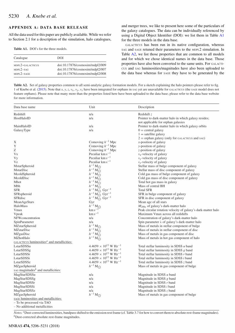
5230 A. Knebe et al.

APP EN D IX A : DATA BASE RELEASE

All the data used for this paper are publicly available. While we referto Section 2.1 for a description of the simulation, halo catalogues,

Table A1. DOI’s for the three models.

Catalogue DOI

MDPL2–GALACTICUS doi:10.17876/cosmosim/mdpl2/009MDPL2–SAG doi:10.17876/cosmosim/mdpl2/007MDPL2–SAGE doi:10.17876/cosmosim/mdpl2/008

and merger trees, we like to present here some of the particulars ofthe galaxy catalogues. The data can be individually referenced byusing a Digital Object Identifier (DOI): we list them in Table A1for the three models in the data base.

GALACTICUS has been run in its native configuration, whereasSAG and SAGE retuned their parameters to the MDPL2 simulation. InTable A2, we list those properties that are common to all modelsand for which we chose identical names in the data base. Thoseproperties have also been converted to the same units. For GALACTI-CUS and SAG luminosities/magnitudes have also been uploaded tothe data base whereas for SAGE they have to be generated by the

Table A2. Set of galaxy properties common to all semi-analytic galaxy formation models. For a sketch explaining the halo pointers please refer to fig.1 of Knebe et al. (2015). Note that x, y, z, vx, vy, vz have been integrated for orphans in SAG yet are unavailable for GALACTICUS (the SAGE model does notfeature orphans). Please note that many more than the properties listed here have been uploaded to the data base; please refer to the data base websitefor more information.

Data base name Unit Description

Redshift n/a Redshift zHostHaloID n/a Pointer to dark-matter halo in which galaxy resides;

not applicable for orphan galaxiesMainHaloID n/a Pointer to dark-matter halo in which galaxy orbitsGalaxyType n/a 0 = central galaxy

1 = satellite galaxy2 = orphan galaxy (only for GALACTICUS and SAG)

X Comoving h−1 Mpc x-position of galaxyY Comoving h−1 Mpc y-position of galaxyZ Comoving h−1 Mpc z-position of galaxyVx Peculiar km s−1 vx-velocity of galaxyVy Peculiar km s−1 vy-velocity of galaxyVz Peculiar km s−1 vz-velocity of galaxyMstarSpheroid h−1 M⊙ Stellar mass of bulge component of galaxyMstarDisc h−1 M⊙ Stellar mass of disc component of galaxyMcoldSpheroid h−1 M⊙ Cold gas mass of bulge component of galaxyMcoldDisc h−1 M⊙ Cold gas mass of disc component of galaxyMhot h−1 M⊙ Total hot gas mass in galaxyMbh h−1 M⊙ Mass of central BHSFR h−1 M⊙ Gyr−1 Total SFRSFRspheroid h−1 M⊙ Gyr−1 SFR in bulge component of galaxySFRdisc h−1 M⊙ Gyr−1 SFR in disc component of galaxyMeanAgeStars Gyr Mean age of all starsHaloMass h−1 M⊙ M200c of galaxy’s dark-matter haloVmax km s−1 Peak circular rotation velocity of galaxy’s dark-matter haloVpeak km s−1 Maximum Vmax across all redshiftsNFWconcentration n/a Concentration of galaxy’s dark-matter haloSpinParameter n/a Spin parameter λ of galaxy’s dark-matter haloMZstarSpheroid h−1 M⊙ Mass of metals in stellar component of bulgeMZstarDisc h−1 M⊙ Mass of metals in stellar component of discMZgasDisc h−1 M⊙ Mass of metals in gas component of discMZhotHalo h−1 M⊙ Mass of metals in hot gas component of haloGALACTICUS luminositiesa and metallicities:LstarSDSSu 4.4659 × 1013 W Hz−1 Total stellar luminosity in SDSS u bandLstarSDSSg 4.4659 × 1013 W Hz−1 Total stellar luminosity in SDSS g bandLstarSDSSr 4.4659 × 1013 W Hz−1 Total stellar luminosity in SDSS r bandLstarSDSSi 4.4659 × 1013 W Hz−1 Total stellar luminosity in SDSS i bandLstarSDSSz 4.4659 × 1013 W Hz−1 Total stellar luminosity in SDSS z bandMZgasSpheroid h−1 M⊙ Mass of metals in gas component of bulgeSAG magnitudesb and metallicities:MagStarSDSSu n/a Magnitude in SDSS u bandMagStarSDSSg n/a Magnitude in SDSS g bandMagStarSDSSr n/a Magnitude in SDSS r bandMagStarSDSSi n/a Magnitude in SDSS i bandMagStarSDSSz n/a Magnitude in SDSS z bandMZgasSpheroid h−1 M⊙ Mass of metals in gas component of bulgeSAGE luminosities and metallicities:– To be processed via TAO– No additional metallicities

Notes. aDust-corrected luminosities, bandpass shifted to the emission rest frame (cf. Table 3.7 for how to convert them to absolute rest-frame magnitudes).bDust-corrected absolute rest-frame magnitudes.

MNRAS 474, 5206–5231 (2018)

Dow

nloaded from https://academ

ic.oup.com/m

nras/article-abstract/474/4/5206/4494373 by Konkoly Observatory user on 23 Septem

ber 2019

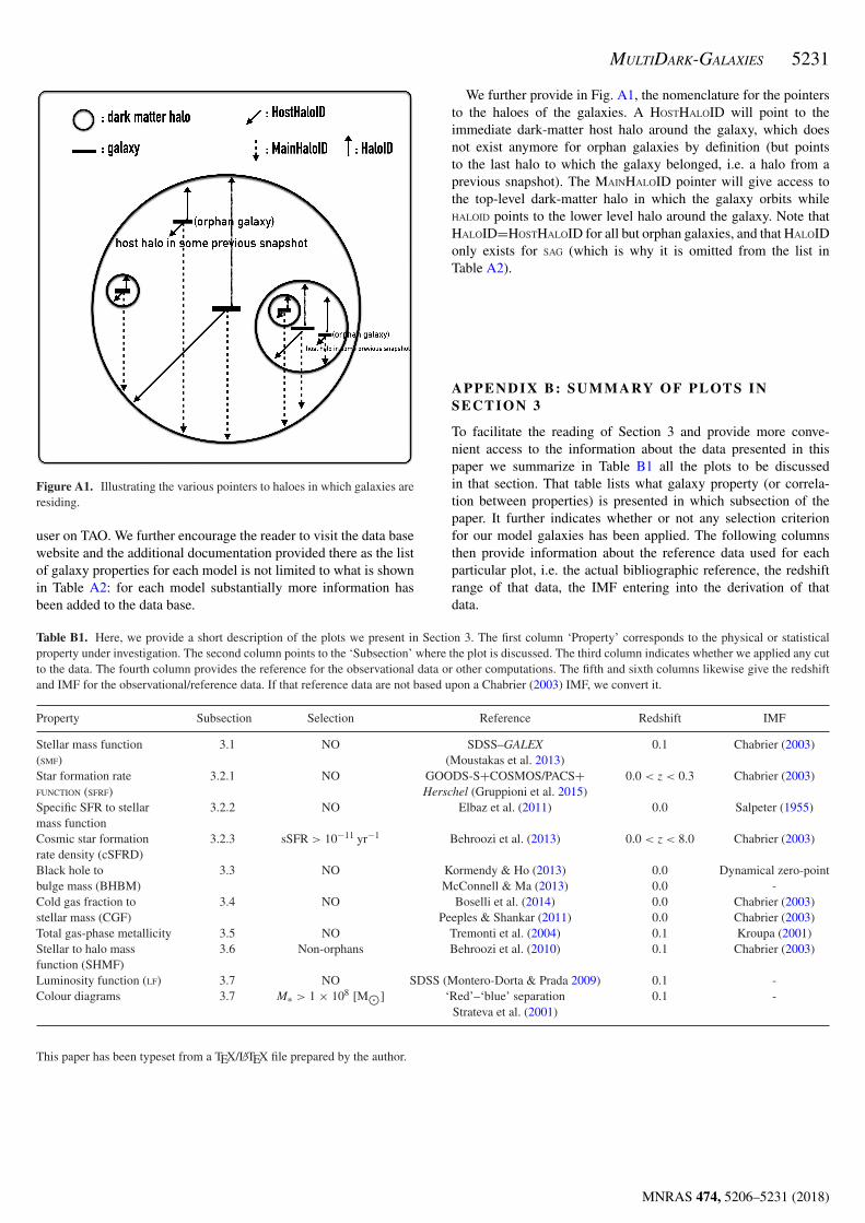
MULTIDARK-GALAXIES 5231

Figure A1. Illustrating the various pointers to haloes in which galaxies areresiding.

user on TAO. We further encourage the reader to visit the data basewebsite and the additional documentation provided there as the listof galaxy properties for each model is not limited to what is shownin Table A2: for each model substantially more information hasbeen added to the data base.

We further provide in Fig. A1, the nomenclature for the pointersto the haloes of the galaxies. A HOSTHALOID will point to theimmediate dark-matter host halo around the galaxy, which doesnot exist anymore for orphan galaxies by definition (but pointsto the last halo to which the galaxy belonged, i.e. a halo from aprevious snapshot). The MAINHALOID pointer will give access tothe top-level dark-matter halo in which the galaxy orbits whileHALOID points to the lower level halo around the galaxy. Note thatHALOID=HOSTHALOID for all but orphan galaxies, and that HALOIDonly exists for SAG (which is why it is omitted from the list inTable A2).

A P P E N D I X B : SU M M A RY O F P L OT S I NSECTI ON 3

To facilitate the reading of Section 3 and provide more conve-nient access to the information about the data presented in thispaper we summarize in Table B1 all the plots to be discussedin that section. That table lists what galaxy property (or correla-tion between properties) is presented in which subsection of thepaper. It further indicates whether or not any selection criterionfor our model galaxies has been applied. The following columnsthen provide information about the reference data used for eachparticular plot, i.e. the actual bibliographic reference, the redshiftrange of that data, the IMF entering into the derivation of thatdata.

Table B1. Here, we provide a short description of the plots we present in Section 3. The first column ‘Property’ corresponds to the physical or statisticalproperty under investigation. The second column points to the ‘Subsection’ where the plot is discussed. The third column indicates whether we applied any cutto the data. The fourth column provides the reference for the observational data or other computations. The fifth and sixth columns likewise give the redshiftand IMF for the observational/reference data. If that reference data are not based upon a Chabrier (2003) IMF, we convert it.

Property Subsection Selection Reference Redshift IMF

Stellar mass function 3.1 NO SDSS–GALEX 0.1 Chabrier (2003)(SMF) (Moustakas et al. 2013)Star formation rate 3.2.1 NO GOODS-S+COSMOS/PACS+ 0.0 < z < 0.3 Chabrier (2003)FUNCTION (SFRF) Herschel (Gruppioni et al. 2015)Specific SFR to stellar 3.2.2 NO Elbaz et al. (2011) 0.0 Salpeter (1955)mass functionCosmic star formation 3.2.3 sSFR > 10−11 yr−1 Behroozi et al. (2013) 0.0 < z < 8.0 Chabrier (2003)rate density (cSFRD)Black hole to 3.3 NO Kormendy & Ho (2013) 0.0 Dynamical zero-pointbulge mass (BHBM) McConnell & Ma (2013) 0.0 -Cold gas fraction to 3.4 NO Boselli et al. (2014) 0.0 Chabrier (2003)stellar mass (CGF) Peeples & Shankar (2011) 0.0 Chabrier (2003)Total gas-phase metallicity 3.5 NO Tremonti et al. (2004) 0.1 Kroupa (2001)Stellar to halo mass 3.6 Non-orphans Behroozi et al. (2010) 0.1 Chabrier (2003)function (SHMF)Luminosity function (LF) 3.7 NO SDSS (Montero-Dorta & Prada 2009) 0.1 -Colour diagrams 3.7 M∗ > 1 × 108 [M⊙] ‘Red’–‘blue’ separation 0.1 -

Strateva et al. (2001)

This paper has been typeset from a TEX/LATEX file prepared by the author.

MNRAS 474, 5206–5231 (2018)

Dow

nloaded from https://academ

ic.oup.com/m

nras/article-abstract/474/4/5206/4494373 by Konkoly Observatory user on 23 Septem

ber 2019

4 Paper II – Luminous red galaxiesand their correlation withenvironment

Publication

Title: A semi-analytical perspective on massive galaxies at z ∼ 0.55

Reference: Monthly Notices of the Royal Astronomical Society, Volume 486, Issue1, p.1316-1331

Date: June 2019

Motivation

The most luminous and massive galaxies in the Universe serve as powerful probes to study theformation of structure, the assembly of mass and cosmology, but their detailed formation andevolution, especially their connection to feedback processes, quenching of star formation or theassembly bias is still not sufficiently understood or quantified [274, 291]. The Sloan DigitalSky Survey SDSS-III/Baryon Oscillation Spectroscopic Survey [BOSS, 88, 99, 244] is a well-studied studied sample of ∼ 1.5 million luminous red galaxies (LRGs) and was used to probethe large-scale distribution of red and passive galaxies in the Universe.

Semi-analytical models have been proven to be a resourceful tool to generate huge sets of galaxyproperties and have been used recently in various frameworks to study e.g. the correlation func-tions and galaxy clustering [46, 103, 283] or the galaxy-halo connection [66, 67]. In Chapter 3we have shown that particularly the SAM Galacticus, from The MultiDark-Galaxies,provides reasonable results on key galaxy properties and clustering functions and therefore weadopt this SAM as our preferred model to study LRGs. Furthermore, Galacticus also providesreasonable outputs on luminosities and colours to reproduce the photometric sample selection ofBOSS-CMASS galaxies. In what follows we present an extensive study of modelled LRGs regard-ing their clustering, halo occupation distribution, and environment affiliation as well as provideprospects on future studies as their assembly history or the detection of the galaxy assemblybias.

55

MNRAS 486, 1316–1331 (2019) doi:10.1093/mnras/stz797Advance Access publication 2019 March 19

A semi-analytical perspective on massive galaxies at z ∼ 0.55

D. Stoppacher ,1,2‹† F. Prada,3 A. D. Montero-Dorta,4 S. Rodrıguez-Torres,2

A. Knebe ,2,5,6 G. Favole ,7 W. Cui ,2,8 A. J. Benson ,9 C. Behrens10

and A. A. Klypin11

1Instituto de Fısica Teorica, (UAM/CSIC), Universidad Autonoma de Madrid, Cantoblanco, E-28049 Madrid, Spain2Departamento de Fısica Teorica, Modulo 15, Facultad de Ciencias, Universidad Autonoma de Madrid, E-28049 Madrid, Spain3Instituto de Astrofısica de Andalucıa (CSIC), Glorieta de la Astronomıa, E-18080 Granada, Spain4Departamento de Fısica Matematica, Instituto de Fısica, Universidade de Sao Paulo, Rua do Matao 1371, Sao Paulo CEP 05508-090, Brazil5Centro de Investigacion Avanzada en Fısica Fundamental (CIAFF), Facultad de Ciencias, Universidad Autonoma de Madrid, E-28049 Madrid, Spain6International Centre for Radio Astronomy Research, University of Western Australia, 35 Stirling Highway, Crawley, Western Australia 6009, Australia7European Space Astronomy Centre (ESAC), Villanueva de la Canada, E-28692 Madrid, Spain8Institute for Astronomy, University of Edinburgh, Royal Observatory, Edinburgh EH9 3HJ, UK9Institut fur Astrophysik, Georg-August Universitat Gottingen, Friedrich-Hund-Platz 1, D-37077 Gottingen, Germany10Carnegie Observatories, 813 Santa Barbara Street, Pasadena, CA 91101, USA11Astronomy Department, New Mexico State University, Dept.4500, Las Cruces, NM 88003-0001, USA

Accepted 2019 March 14. Received 2019 March 13; in original form 2018 December 20

ABSTRACTThe most massive and luminous galaxies in the Universe serve as powerful probes to studythe formation of structure, the assembly of mass, and cosmology. However, their detailedformation and evolution is still barely understood. Here we extract a sample of massivemock galaxies from the semi-analytical model of galaxy formation (SAM) GALACTICUS fromthe MULTIDARK-GALAXIES by replicating the CMASS photometric selection from the SDSS-III Baryon Oscillation Spectroscopic Survey (BOSS). The comparison of the GALACTICUS

CMASS-mock with BOSS–CMASS data allows us to explore different aspects of the massivegalaxy population at 0.5 < z < 0.6, including the galaxy–halo connection and the galaxyclustering. We find good agreement between our modelled galaxies and observations regardingthe galaxy–halo connection, but our CMASS-mock overestimates the clustering amplitudeof the two-point correlation function due to a smaller number density compared to BOSS,a lack of blue objects, and a small intrinsic scatter in stellar mass at fixed halo mass of<0.1 dex. To alleviate this problem, we construct an alternative mock catalogue mimickingthe CMASS colour–magnitude distribution by randomly down-sampling the SAM catalogue.This CMASS-mock reproduces the clustering of CMASS galaxies within 1σ and showssome environmental dependency of star formation properties that could be connected tothe quenching of star formation and the assembly bias.

Key words: galaxies: evolution – galaxies: haloes – cosmology: theory – dark matter.

1 IN T RO D U C T I O N

The most luminous and massive galaxies in the Universe serve aspowerful probes to study the formation of structure, the assemblyof mass and cosmology, but their detailed formation and evolution,especially their connection to feedback processes, quenching of starformation, or the assembly bias is still not sufficiently understood orquantified (Tinker et al. 2013; Wechsler & Tinker 2018). The Sloan

⋆ E-mail: doris.stoppacher@csic.es† Severo Ochoa IFT-CSIC Scholar.

Digital Sky Survey SDSS-III/Baryon Oscillation SpectroscopicSurvey (BOSS, Schlegel, White & Eisenstein 2009; Eisenstein et al.2011; Dawson et al. 2013) was dedicated to studying properties ofthe large-scale distribution of massive galaxies and provides a well-studied sample of ∼1.5 million luminous red galaxies (LRGs). TheBOSS sample is divided into two: a low-redshift (LOWZ) and a high-redshift sample (CMASS, stands for ‘constant mass’), respectively.

The CMASS sample covers a wide redshift in the range 0.43 <

z < 0.75 exhibiting a peak in comoving number density of n ∼3.4 × 10−4 h3Mpc−3 at z ∼ 0.5. The stellar mass function (SMF)evolves very little in this redshift range suggesting that CMASSgalaxies are passive and show almost no ongoing star formation

C⃝ 2019 The Author(s)Published by Oxford University Press on behalf of the Royal Astronomical Society

Dow

nloaded from https://academ

ic.oup.com/m

nras/article-abstract/486/1/1316/5393411 by MTA C

SFK CSI user on 23 Septem

ber 2019

SAM CMASS-mocks 1317

(Maraston et al. 2013). A non-evolving sample of massive galaxiesprovides an excellent ‘cosmic laboratory’ to study galaxy formationand evolution as shown by Bernardi et al. (2016), Montero-Dortaet al. (2016), and Montero-Dorta, Bolton & Shu (2017a), andtheir link to cosmology via e.g. the large-scale structure (LSS)distribution and clustering of BOSS galaxies studied by Chuanget al. (2016), Rodrıguez-Torres et al. (2016), and Guo, Yang & Lu(2018).BOSSLRGs were repeatedly used to determine fundamentalcosmological parameters (Cuesta et al. 2016; Gil-Marın et al. 2017;Ross et al. 2017) and to put cosmological models to the test (e.g.Anderson et al. 2014; Beutler et al. 2014; Alam, Ata & Bailey2017; Sullivan, Wiegand & Eisenstein 2017; Mueller et al. 2018).Furthermore, because the sample addresses the most luminous andred galaxies, they act as an important probe to close the gap inunderstanding the link between dark matter haloes and massivegalaxies (Leauthaud et al. 2012; Nuza et al. 2013; Guo et al. 2014;Favole et al. 2016; Saito et al. 2016).

At low redshift LRGs are known to populate the most massivehaloes located in denser regions such as the centre of clusters andsuperclusters (Lietzen et al. 2012). That makes them particularlyinteresting to study, because they give clues to the assembly ofthe most massive structures, the formation of haloes, and theirconnection to their associated galaxies. Thereby the ratio of theirstellar to halo masses as a function of halo mass (SHMF) allowsfor exploring the galaxy–halo connection and the formation andevolution of those galaxies in dark matter haloes of a certainmass range. Or equally, what halo mass is related to a galaxy thatproduced a certain stellar mass over a certain time. From a morecosmological point of view the relation shows how galaxies tracedark matter and how its density field is distributed.1 Interestingly,the haloes at intermediate masses produce stars most efficiently,relative to their mass (White & Frenk 1991; Benson et al. 2003;Bower et al. 2006). It is still barely understood why haloes withlower or higher masses are by orders of magnitudes less efficient(Behroozi, Wechsler & Conroy 2013). To shed light on this topicone would need to study the full history of mass assembly andstar formation within a large redshift range, which is a costly taskfor ‘full-physics’ hydro-cosmological simulations. The number ofparticles in question to cover a similar physical volume and amountof galaxies as an observational survey is therefore inaccessible.Different approaches to modelling the population of dark matterhaloes with galaxies as well as their formation and evolution insidethe haloes have been developed. One of them being semi-analyticalmodels (hereafter SAMs). SAMs are usually build upon N-bodydark matter simulations (e.g MILLENNIUM: Springel et al. 2005,MULTIDARK: Klypin et al. 2016) using merger trees (information ofthe hierarchical formation of dark matter haloes) and implementingbaryonic physics as a post-processing step. For details on semi-analytical modelling we refer to excellent reviews on the field(Baugh 2006; Benson 2010; Baugh 2013; Somerville & Dave 2015;Cora 2016).

SAMs have been used recently in various frameworks to studye.g. correlation functions and galaxy clustering (Campbell et al.2015; Farrow et al. 2015; van Daalen et al. 2016), the galaxy–haloconnection (Contreras et al. 2013, 2015), or active galactic nuclei,galaxy mergers, and the cosmic web (Almeida et al. 2008; Liu et al.

1From the density field the corresponding power spectrum can be con-structed and from that cosmological parameter determined. One can seethat this simple relation between stellar and halo mass is indeed a powerfulconstraint.

2016; Ren, Trenti & Mutch 2018; Shirakata et al. 2018). They havebeen utilized to trace the star formation history (Mutch, Poole &Croton 2013; Lagos et al. 2014; Orsi et al. 2014; Gruppioni et al.2015) to understand the galaxy mass–luminosity relations (Zoldanet al. 2018), or the processes regulating star formation (Henriqueset al. 2017, 2018; Cora et al. 2018), or generating galaxy coloursand metallicities (Yates, Kauffmann & Guo 2012; Gonzalez-Perezet al. 2014; Rodrigues, Vernon & Bower 2017; Xie et al. 2017;Collacchioni et al. 2018).

Within this paper we connect two major frameworks using aSAM: galaxy clustering and galaxy formation, in order to learnabout the nature and properties of those most massive galaxies.Contreras et al. (2013) performed a similar work and claimed thatgalaxy properties, apart from the stellar mass, e.g. star formationrate or cold gas mass, have more complicated correlation and non-negligible impacts on the clustering. Thereby the type of galaxy(central or satellite) plays a crucial role. Knebe et al. (2018)did a similar study with the MULTIDARK-SAMs for the SDSSmain sample (z ∼ 0.1). Within our work we expand upon thesestudies focusing at the redshift z ∼ 0.5 and CMASS galaxies. Forthat we use the same publicly available galaxy catalogues calledthe ‘MULTIDARK-GALAXIES’. From them we take the SAM-codeGALACTICUS as our modelled galaxy catalogue because it providesproper luminosities in the SDSS ugriz-band magnitudes suitable tocompare with data from BOSS (Data Release 12), which we adoptas our observational sample.

This paper is organized as follows: in Section 2 we describe theobservational and modelled galaxy samples. In Section 3 we showhow to replicate the CMASS photometric selection for our model,GALACTICUS. We further provide confidence plots and a detailedstudy of various galaxy properties in Section 4. Our results anddiscussion can be found in Sections 5 and 6, respectively, and oursummary in Section 7. The adopted cosmology in the MULTIDARK-GALAXIES as well as in this paper consists of a flat Lambdacold dark matter (#CDM) model with the following cosmo-logical parameters: $m = 0.307, $b = 0.048, $# = 0.693, σ8 =0.823, ns = 0.96, and a dimensionless Hubble parameter h = 0.678(Planck Collaboration 2015). Hereafter, h will be absorbed in thenumerical value of its property throughout the text and in all tablesand figures.

2 DATA SE T S A N D SE L E C T I O N

We use BOSS–CMASS galaxies as our observational and the semi-analytical MDPL2-Galacticus galaxy catalogue product asour modelled data sample. In this section we show the selectionalgorithms used to generate those samples. We further documentall necessary assumptions and corrections applied to the samplesin order to create comparable observational and modelled datasets. Those corrections include e.g. adjusting galaxy properties toour chosen cosmology (observations) or generating colours fromluminosities (model).

2.1 Observational data: the BOSS–CMASS sample

The CMASS sample was designed to target the most LRGs in orderto produce a uniformly (in mass) distributed samples of galaxies atredshift 0.43 < z < 0.7 by applying a set of colour–magnitude cutsequations (1)–(8) shown below. The CMASS selection is similar tothe algorithms used to target SDSS-I/II Cut-II (Eisensteinet al. 2001) and 2SLAQ LRGs (Cannon et al. 2006), using (g− i) and (r − i) colours to isolate high-redshift galaxies, but the

MNRAS 486, 1316–1331 (2019)

Dow

nloaded from https://academ

ic.oup.com/m

nras/article-abstract/486/1/1316/5393411 by MTA C

SFK CSI user on 23 Septem

ber 2019

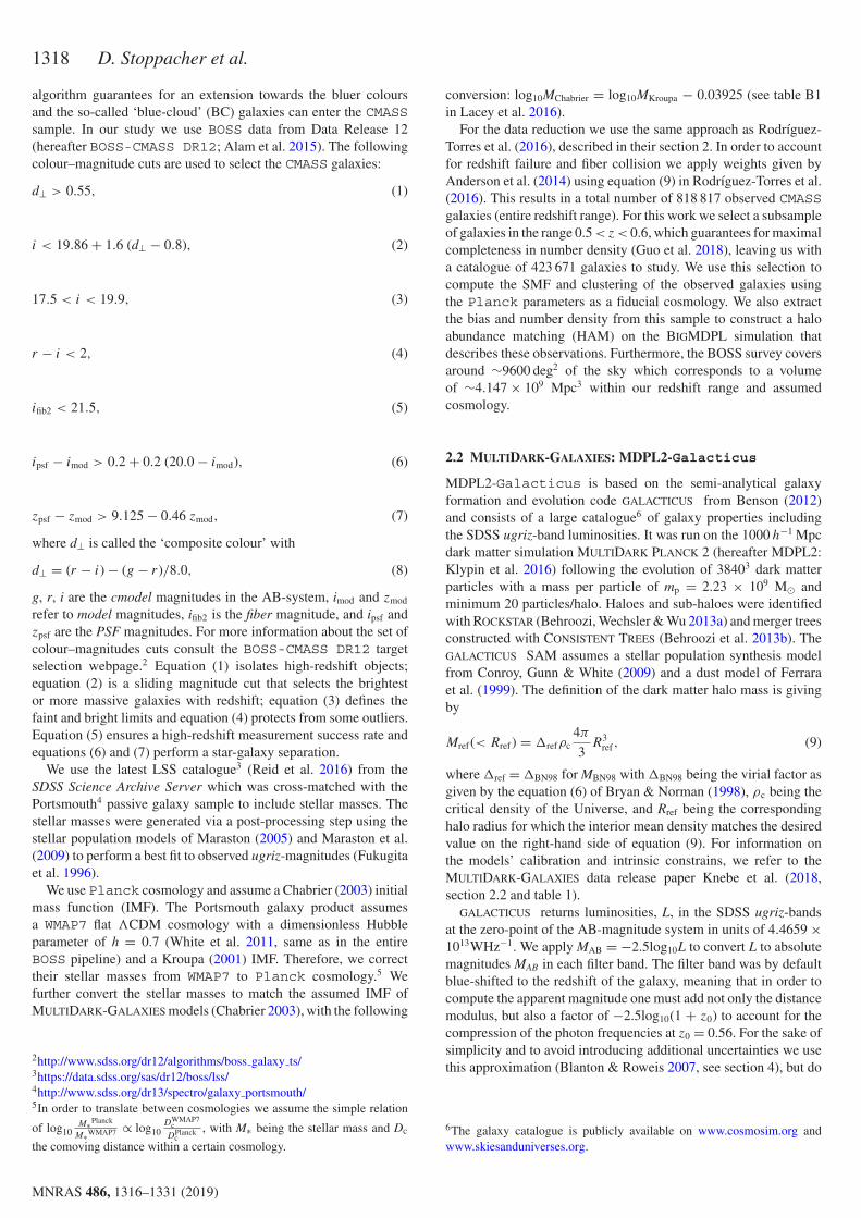
1318 D. Stoppacher et al.

algorithm guarantees for an extension towards the bluer coloursand the so-called ‘blue-cloud’ (BC) galaxies can enter the CMASSsample. In our study we use BOSS data from Data Release 12(hereafter BOSS-CMASS DR12; Alam et al. 2015). The followingcolour–magnitude cuts are used to select the CMASS galaxies:

d⊥ > 0.55, (1)

i < 19.86 + 1.6 (d⊥− 0.8), (2)

17.5 < i < 19.9, (3)

r − i < 2, (4)

ifib2 < 21.5, (5)

ipsf − imod > 0.2 + 0.2 (20.0 − imod), (6)

zpsf − zmod > 9.125 − 0.46 zmod, (7)

where d⊥ is called the ‘composite colour’ with

d⊥ = (r − i) − (g − r)/8.0, (8)

g, r, i are the cmodel magnitudes in the AB-system, imod and zmod

refer to model magnitudes, ifib2 is the fiber magnitude, and ipsf andzpsf are the PSF magnitudes. For more information about the set ofcolour–magnitudes cuts consult the BOSS-CMASS DR12 targetselection webpage.2 Equation (1) isolates high-redshift objects;equation (2) is a sliding magnitude cut that selects the brightestor more massive galaxies with redshift; equation (3) defines thefaint and bright limits and equation (4) protects from some outliers.Equation (5) ensures a high-redshift measurement success rate andequations (6) and (7) perform a star-galaxy separation.

We use the latest LSS catalogue3 (Reid et al. 2016) from theSDSS Science Archive Server which was cross-matched with thePortsmouth4 passive galaxy sample to include stellar masses. Thestellar masses were generated via a post-processing step using thestellar population models of Maraston (2005) and Maraston et al.(2009) to perform a best fit to observed ugriz-magnitudes (Fukugitaet al. 1996).

We use Planck cosmology and assume a Chabrier (2003) initialmass function (IMF). The Portsmouth galaxy product assumesa WMAP7 flat #CDM cosmology with a dimensionless Hubbleparameter of h = 0.7 (White et al. 2011, same as in the entireBOSS pipeline) and a Kroupa (2001) IMF. Therefore, we correcttheir stellar masses from WMAP7 to Planck cosmology.5 Wefurther convert the stellar masses to match the assumed IMF ofMULTIDARK-GALAXIES models (Chabrier 2003), with the following

2http://www.sdss.org/dr12/algorithms/boss galaxy ts/3https://data.sdss.org/sas/dr12/boss/lss/4http://www.sdss.org/dr13/spectro/galaxy portsmouth/5In order to translate between cosmologies we assume the simple relation

of log10M∗Planck

M∗WMAP7 ∝ log10DWMAP7

cDPlanck

c, with M∗ being the stellar mass and Dc

the comoving distance within a certain cosmology.

conversion: log10MChabrier = log10MKroupa − 0.03925 (see table B1in Lacey et al. 2016).

For the data reduction we use the same approach as Rodrıguez-Torres et al. (2016), described in their section 2. In order to accountfor redshift failure and fiber collision we apply weights given byAnderson et al. (2014) using equation (9) in Rodrıguez-Torres et al.(2016). This results in a total number of 818 817 observed CMASSgalaxies (entire redshift range). For this work we select a subsampleof galaxies in the range 0.5 < z < 0.6, which guarantees for maximalcompleteness in number density (Guo et al. 2018), leaving us witha catalogue of 423 671 galaxies to study. We use this selection tocompute the SMF and clustering of the observed galaxies usingthe Planck parameters as a fiducial cosmology. We also extractthe bias and number density from this sample to construct a haloabundance matching (HAM) on the BIGMDPL simulation thatdescribes these observations. Furthermore, the BOSS survey coversaround ∼9600 deg2 of the sky which corresponds to a volumeof ∼4.147 × 109 Mpc3 within our redshift range and assumedcosmology.

2.2 MULTIDARK-GALAXIES: MDPL2-Galacticus

MDPL2-Galacticus is based on the semi-analytical galaxyformation and evolution code GALACTICUS from Benson (2012)and consists of a large catalogue6 of galaxy properties includingthe SDSS ugriz-band luminosities. It was run on the 1000 h−1 Mpcdark matter simulation MULTIDARK PLANCK 2 (hereafter MDPL2:Klypin et al. 2016) following the evolution of 38403 dark matterparticles with a mass per particle of mp = 2.23 × 109 M⊙ andminimum 20 particles/halo. Haloes and sub-haloes were identifiedwith ROCKSTAR (Behroozi, Wechsler & Wu 2013a) and merger treesconstructed with CONSISTENT TREES (Behroozi et al. 2013b). TheGALACTICUS SAM assumes a stellar population synthesis modelfrom Conroy, Gunn & White (2009) and a dust model of Ferraraet al. (1999). The definition of the dark matter halo mass is givingby

Mref (< Rref ) = %refρc4π

3R3

ref, (9)

where %ref = %BN98 for MBN98 with %BN98 being the virial factor asgiven by the equation (6) of Bryan & Norman (1998), ρc being thecritical density of the Universe, and Rref being the correspondinghalo radius for which the interior mean density matches the desiredvalue on the right-hand side of equation (9). For information onthe models’ calibration and intrinsic constrains, we refer to theMULTIDARK-GALAXIES data release paper Knebe et al. (2018,section 2.2 and table 1).

GALACTICUS returns luminosities, L, in the SDSS ugriz-bandsat the zero-point of the AB-magnitude system in units of 4.4659 ×1013WHz−1. We apply MAB = −2.5log10L to convert L to absolutemagnitudes MAB in each filter band. The filter band was by defaultblue-shifted to the redshift of the galaxy, meaning that in order tocompute the apparent magnitude one must add not only the distancemodulus, but also a factor of −2.5log10(1 + z0) to account for thecompression of the photon frequencies at z0 = 0.56. For the sake ofsimplicity and to avoid introducing additional uncertainties we usethis approximation (Blanton & Roweis 2007, see section 4), but do

6The galaxy catalogue is publicly available on www.cosmosim.org andwww.skiesanduniverses.org.

MNRAS 486, 1316–1331 (2019)

Dow

nloaded from https://academ

ic.oup.com/m

nras/article-abstract/486/1/1316/5393411 by MTA C

SFK CSI user on 23 Septem

ber 2019

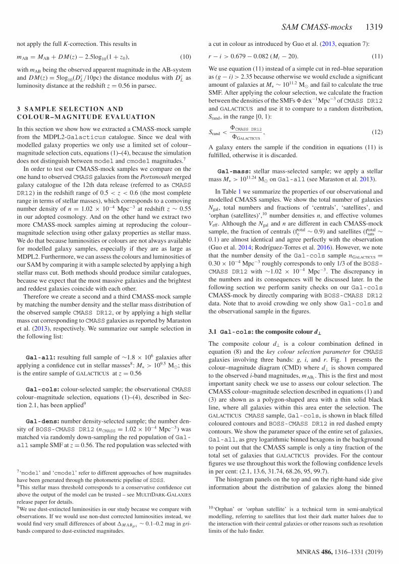
SAM CMASS-mocks 1319

not apply the full K-correction. This results in

mAB = MAB + DM(z) − 2.5log10(1 + z0), (10)

with mAB being the observed apparent magnitude in the AB-systemand DM(z) = 5log10(Dz

L/10pc) the distance modulus with DzL as

luminosity distance at the redshift z = 0.56 in parsec.

3 SA M P L E SE L E C T I O N A N DC O L O U R – M AG N I T U D E E VA L UAT I O N

In this section we show how we extracted a CMASS-mock samplefrom the MDPL2-Galacticus catalogue. Since we deal withmodelled galaxy properties we only use a limited set of colour–magnitude selection cuts, equations (1)–(4), because the simulationdoes not distinguish between model and cmodel magnitudes.7

In order to test our CMASS-mock samples we compare on theone hand to observed CMASS galaxies from the Portsmouth mergedgalaxy catalogue of the 12th data release (referred to as CMASSDR12) in the redshift range of 0.5 < z < 0.6 (the most completerange in terms of stellar masses), which corresponds to a comovingnumber density of n = 1.02 × 10−4 Mpc−3 at redshift z ∼ 0.55in our adopted cosmology. And on the other hand we extract twomore CMASS-mock samples aiming at reproducing the colour–magnitude selection using other galaxy properties as stellar mass.We do that because luminosities or colours are not always availablefor modelled galaxy samples, especially if they are as large asMDPL2. Furthermore, we can assess the colours and luminosities ofour SAM by comparing it with a sample selected by applying a highstellar mass cut. Both methods should produce similar catalogues,because we expect that the most massive galaxies and the brightestand reddest galaxies coincide with each other.

Therefore we create a second and a third CMASS-mock sampleby matching the number density and the stellar mass distribution ofthe observed sample CMASS DR12, or by applying a high stellarmass cut corresponding to CMASS galaxies as reported by Marastonet al. (2013), respectively. We summarize our sample selection inthe following list:

Gal-all: resulting full sample of ∼1.8 × 106 galaxies afterapplying a confidence cut in stellar masses8: M∗ > 109.5 M⊙; thisis the entire sample of GALACTICUS at z = 0.56

Gal-cols: colour-selected sample; the observational CMASScolour–magnitude selection, equations (1)–(4), described in Sec-tion 2.1, has been applied9

Gal-dens: number density-selected sample; the number den-sity of BOSS-CMASS DR12 (nCMASS = 1.02 × 10−4 Mpc−3) wasmatched via randomly down-sampling the red population of Gal-all sample SMF at z = 0.56. The red population was selected with

7‘model’ and ‘cmodel’ refer to different approaches of how magnitudeshave been generated through the photometric pipeline of SDSS.8This stellar mass threshold corresponds to a conservative confidence cutabove the output of the model can be trusted – see MULTIDARK-GALAXIES

release paper for details.9We use dust-extincted luminosities in our study because we compare withobservations. If we would use non-dust corrected luminosities instead, wewould find very small differences of about %MABgri ∼ 0.1–0.2 mag in gri-bands compared to dust-extincted magnitudes.

a cut in colour as introduced by Guo et al. (2013, equation 7):

r − i > 0.679 − 0.082 (Mi − 20). (11)

We use equation (11) instead of a simple cut in red–blue separationas (g − i) > 2.35 because otherwise we would exclude a significantamount of galaxies at M∗ ∼ 1011.2 M⊙ and fail to calculate the trueSMF. After applying the colour selection, we calculate the fractionbetween the densities of the SMFs ( dex−1Mpc−3 ofCMASS DR12and GALACTICUS and use it to compare to a random distribution,Srand, in the range [0, 1):

Srand <(CMASS DR12

(GALACTICUS

, (12)

A galaxy enters the sample if the condition in equations (11) isfulfilled, otherwise it is discarded.

Gal-mass: stellar mass-selected sample; we apply a stellarmass M∗ > 1011.24 M⊙ on Gal-all (see Maraston et al. 2013).

In Table 1 we summarize the properties of our observational andmodelled CMASS samples. We show the total number of galaxiesNgal, total numbers and fractions of ‘centrals’, ‘satellites’, and‘orphan (satellites)’,10 number densities n, and effective volumesVeff. Although the Ngal and n are different in each CMASS-mocksample, the fraction of centrals (ftotal

c ∼ 0.9) and satellites (ftotalsats ∼

0.1) are almost identical and agree perfectly with the observation(Guo et al. 2014; Rodrıguez-Torres et al. 2016). However, we notethat the number density of the Gal-cols sample nGALACTICUS =0.30 × 10−4 Mpc−3 roughly corresponds to only 1/3 of the BOSS-CMASS DR12 with ∼1.02 × 10−4 Mpc−3. The discrepancy inthe numbers and its consequences will be discussed later. In thefollowing section we perform sanity checks on our Gal-colsCMASS-mock by directly comparing with BOSS-CMASS DR12data. Note that to avoid crowding we only show Gal-cols andthe observational sample in the figures.

3.1 Gal-cols: the composite colour d⊥

The composite colour d⊥ is a colour combination defined inequation (8) and the key colour selection parameter for CMASSgalaxies involving three bands: g, i, and r. Fig. 1 presents thecolour–magnitude diagram (CMD) where d⊥ is shown comparedto the observed i-band magnitudes, mABi . This is the first and mostimportant sanity check we use to assess our colour selection. TheCMASS colour–magnitude selection described in equations (1) and(3) are shown as a polygon-shaped area with a thin solid blackline, where all galaxies within this area enter the selection. TheGALACTICUS CMASS sample, Gal-cols, is shown in black filledcoloured contours and BOSS-CMASS DR12 in red dashed emptycontours. We show the parameter space of the entire set of galaxies,Gal-all, as grey logarithmic binned hexagons in the backgroundto point out that the CMASS sample is only a tiny fraction of thetotal set of galaxies that GALACTICUS provides. For the contourfigures we use throughout this work the following confidence levelsin per cent: (2.1, 13.6, 31.74, 68.26, 95, 99.7).

The histogram panels on the top and on the right-hand side giveinformation about the distribution of galaxies along the binned

10‘Orphan’ or ‘orphan satellite’ is a technical term in semi-analyticalmodelling, referring to satellites that lost their dark matter haloes due tothe interaction with their central galaxies or other reasons such as resolutionlimits of the halo finder.

MNRAS 486, 1316–1331 (2019)

Dow

nloaded from https://academ

ic.oup.com/m

nras/article-abstract/486/1/1316/5393411 by MTA C

SFK CSI user on 23 Septem

ber 2019

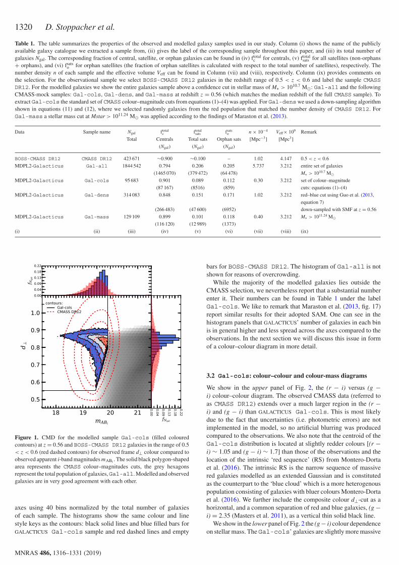
1320 D. Stoppacher et al.

Table 1. The table summarizes the properties of the observed and modelled galaxy samples used in our study. Column (i) shows the name of the publiclyavailable galaxy catalogue we extracted a sample from, (ii) gives the label of the corresponding sample throughout this paper, and (iii) its total number ofgalaxies Ngal. The corresponding fraction of central, satellite, or orphan galaxies can be found in (iv) ftotal

c for centrals, (v) ftotalsats for all satellites (non-orphans

+ orphans), and (vi) fsatso for orphan satellites (the fraction of orphan satellites is calculated with respect to the total number of satellites), respectively. The

number density n of each sample and the effective volume Veff can be found in Column (vii) and (viii), respectively. Column (ix) provides comments onthe selection. For the observational sample we select BOSS-CMASS DR12 galaxies in the redshift range of 0.5 < z < 0.6 and label the sample CMASSDR12. For the modelled galaxies we show the entire galaxies sample above a confidence cut in stellar mass of M∗ > 1010.7 M⊙: Gal-all and the followingCMASS-mock samples: Gal-cols, Gal-dens, and Gal-mass at redshift z = 0.56 (which matches the median redshift of the full CMASS sample). Toextract Gal-cols the standard set of CMASS colour–magnitude cuts from equations (1)–(4) was applied. For Gal-denswe used a down-sampling algorithmshown in equations (11) and (12), where we selected randomly galaxies from the red population that matched the number density of CMASS DR12. ForGal-mass a stellar mass cut at Mstar > 1011.24 M⊙ was applied according to the findings of Maraston et al. (2013).

Data Sample name Ngal ftotalc ftotal

sats fsatso n × 10−4 Veff× 109 Remark

Total Centrals Total sats Orphan sats [Mpc−3] [Mpc3](Ngal) (Ngal) (Ngal)

BOSS-CMASS DR12 CMASS DR12 423 671 ∼0.900 ∼0.100 – 1.02 4.147 0.5 < z < 0.6MDPL2-Galacticus Gal-all 1844 542 0.794 0.206 0.205 5.737 3.212 entire set of galaxies

(1465 070) (379 472) (64 478) M∗ > 1010.7 M⊙

MDPL2-Galacticus Gal-cols 95 683 0.901 0.089 0.112 0.30 3.212 set of colour–magnitude(87 167) (8516) (859) cuts: equations (1)–(4)

MDPL2-Galacticus Gal-dens 314 083 0.848 0.151 0.171 1.02 3.212 red–blue cut using Guo et al. (2013,equation 7)

(266 483) (47 600) (6952) down-sampled with SMF at z = 0.56MDPL2-Galacticus Gal-mass 129 109 0.899 0.101 0.118 0.40 3.212 M∗ > 1011.24 M⊙

(116 120) (12 989) (1373)(i) (ii) (iii) (iv) (v) (vi) (vii) (viii) (ix)

Figure 1. CMD for the modelled sample Gal-cols (filled colouredcontours) at z = 0.56 and BOSS-CMASS DR12 galaxies in the range of 0.5< z < 0.6 (red dashed contours) for observed frame d⊥ colour compared toobserved apparent i-band magnitudes mABi . The solid black polygon-shapedarea represents the CMASS colour–magnitudes cuts, the grey hexagonsrepresent the total population of galaxies,Gal-all. Modelled and observedgalaxies are in very good agreement with each other.

axes using 40 bins normalized by the total number of galaxiesof each sample. The histograms show the same colour and linestyle keys as the contours: black solid lines and blue filled bars forGALACTICUS Gal-cols sample and red dashed lines and empty

bars for BOSS-CMASS DR12. The histogram of Gal-all is notshown for reasons of overcrowding.

While the majority of the modelled galaxies lies outside theCMASS selection, we nevertheless report that a substantial numberenter it. Their numbers can be found in Table 1 under the labelGal-cols. We like to remark that Maraston et al. (2013, fig. 17)report similar results for their adopted SAM. One can see in thehistogram panels that GALACTICUS’ number of galaxies in each binis in general higher and less spread across the axes compared to theobservations. In the next section we will discuss this issue in formof a colour–colour diagram in more detail.

3.2 Gal-cols: colour–colour and colour-mass diagrams

We show in the upper panel of Fig. 2, the (r − i) versus (g −i) colour–colour diagram. The observed CMASS data (referred toas CMASS DR12) extends over a much larger region in the (r −i) and (g − i) than GALACTICUS Gal-cols. This is most likelydue to the fact that uncertainties (i.e. photometric errors) are notimplemented in the model, so no artificial blurring was producedcompared to the observations. We also note that the centroid of theGal-cols distribution is located at slightly redder colours [(r −i) ∼ 1.05 and (g − i) ∼ 1.7] than those of the observations and thelocation of the intrinsic ‘red sequence’ (RS) from Montero-Dortaet al. (2016). The intrinsic RS is the narrow sequence of massivered galaxies modelled as an extended Gaussian and is constitutedas the counterpart to the ‘blue cloud’ which is a more heterogenouspopulation consisting of galaxies with bluer colours Montero-Dortaet al. (2016). We further include the composite colour d⊥-cut as ahorizontal, and a common separation of red and blue galaxies, (g −i) = 2.35 (Masters et al. 2011), as a vertical thin solid black line.

We show in the lower panel of Fig. 2 the (g − i) colour dependenceon stellar mass. TheGal-cols’ galaxies are slightly more massive

MNRAS 486, 1316–1331 (2019)

Dow

nloaded from https://academ

ic.oup.com/m

nras/article-abstract/486/1/1316/5393411 by MTA C

SFK CSI user on 23 Septem

ber 2019

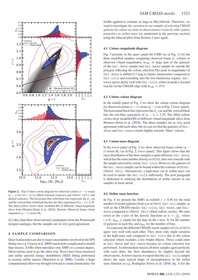
SAM CMASS-mocks 1321

Figure 2. Top: Colour–colour diagram for observed colours (r − i) versus(g − i) for Gal-cols (filled coloured contours) and CMASS DR12 (reddashed contours). The horizontal thin solid black line represents the d⊥-cutand the vertical thin solid black line the red–blue separation of (g − i) = 2.35.The filled yellow circles show modelled RS of different i-band magnitudeslices from Montero-Dorta et al. (2016). Bottom: Observed frame colourseparation (g − i) versus M∗.

(0.2 dex) than their observational counterparts from the Portsmouthmerged catalogue, but the samples are in very good agreement.

4 SA M P L E C O M PA R I S O N

Since luminosities are due to many uncertainties involved in the SPSfitting (see e.g. Conroy et al. 2009) much more complicated to modelthan masses, SAMs often reproduce only SMFs to a certain degree.Observations need to go the other way: fluxes have been measuredand stellar spectral energy distribution (SED) fitting performedto assume stellar masses (Maraston et al. 2006). Usually a hugecomputational effort was brought forward to create luminosities for

SAMs applied to volumes as large as MULTIDARK. Therefore, wewant to investigate the variation in our samples of selecting CMASSgalaxies by colour (as done in observations) versus by other galaxyproperties as stellar mass (as mentioned in the previous section)using the fiducial plots from Section 3 once again.

4.1 Colour–magnitude diagram

Fig. 3 presents in the upper panel the CMD (as in Fig. 1) for thethree modelled samples comparing observed frame d⊥ colours toobserved i-band magnitudes, mABi . A large part of the galaxiesof the Gal-dens sample and Gal-mass sample lie outside thepolygon reflecting the colour selection.The peak in magnitudes ofGal-dens is shifted 0.3 mag to fainter luminosities compared toGal-cols and extending into the low-luminosity regime. Gal-mass agrees pretty well with Gal-cols, where its peak is locatedexactly on the CMASS edge with mABi = 19.9.

4.2 Colour–colour diagram

In the middle panel of Fig. 3 we show the colour–colour diagramfor observed colours (r − i) versus (g − i) (as in Fig. 2 lower panel).The horizontal black line represents the d⊥-cut and the vertical blackline the red–blue separation of (g − i) = 2.35. The filled yellowcircles show modelled RS of different i-band magnitude slices fromMontero-Dorta et al. (2016). The three samples are in very goodagreement with each other, but we can see that the galaxies of Gal-dens and Gal-mass extend slightly towards ‘bluer’ colours.

4.3 Colour-mass diagram

In the lower panel of Fig. 3 we show observed frame colour (g −i) versus M∗ (as in Fig. 2, lower panel). This figure shows that themass distribution of the three samples is quite different.Gal-dens,which has the same number density asBOSS, does not coincide withthe sample selected by colour,Gal-cols. However, the galaxies ofthe Gal-dens sample can be bound within the contours of BOSS-CMASS DR12. Alternatively, a high-mass cut in stellar mass canbe used to mimic the Gal-cols sufficiently. The next paragraphis dedicated to studying the distribution of stellar masses in oursamples in more detail.

4.4 Stellar mass function

In Fig. 4 we present the SMFs at redshift z = 0.56 for the totalnumber of model galaxies from GALACTICUS Gal-all sample, aswell as the CMASS-mocks: Gal-cols, Gal-mass, and Gal-dens compared to CMASS DR12 (filled yellow circles). We stateerrors in the y-axis of the density functions as σi = yi√

N i, where

i = 0...nbins, yi stands for the data on the y-axis, Ni for the numberof galaxies in each bin, and nbins for the number of bins.

As expected, the different CMASS-mock samples of GALACTICUS

agree very well with each other. They show only slight variationat the high-mass end compared to Gal-cols due to the colourselection which excludes a few bright objects. Those could enterin Gal-dens and Gal-mass because no colour selection wasperformed. At intermediate masses all three samples agree perfectlywith each other, but their abundances lie slightly beyond theobservations. At lower masses we report that theGal-cols sampleshows the same typical shape of incompleteness in the stellarmass function as e.g. Rodrıguez-Torres et al. (2016, fig. 3) for the

MNRAS 486, 1316–1331 (2019)

Dow

nloaded from https://academ

ic.oup.com/m

nras/article-abstract/486/1/1316/5393411 by MTA C

SFK CSI user on 23 Septem

ber 2019

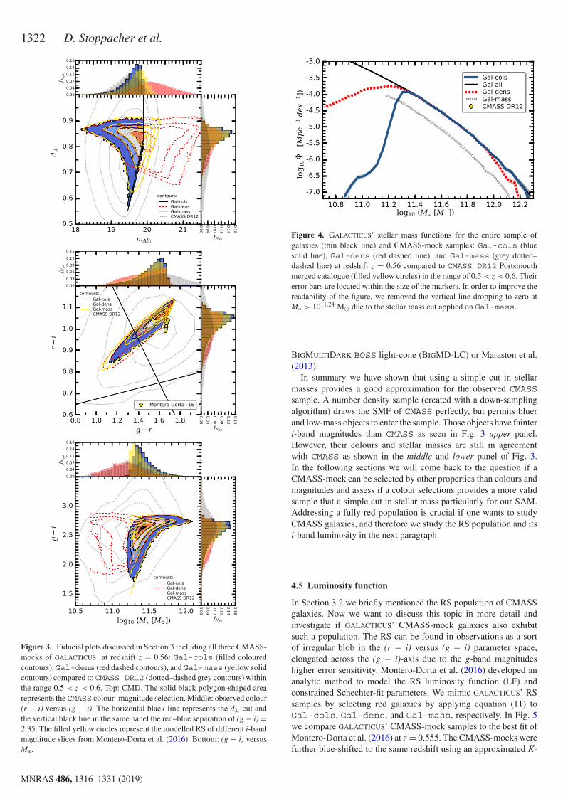
1322 D. Stoppacher et al.

Figure 3. Fiducial plots discussed in Section 3 including all three CMASS-mocks of GALACTICUS at redshift z = 0.56: Gal-cols (filled colouredcontours), Gal-dens (red dashed contours), and Gal-mass (yellow solidcontours) compared to CMASS DR12 (dotted–dashed grey contours) withinthe range 0.5 < z < 0.6. Top: CMD. The solid black polygon-shaped arearepresents the CMASS colour–magnitude selection. Middle: observed colour(r − i) versus (g − i). The horizontal black line represents the d⊥-cut andthe vertical black line in the same panel the red–blue separation of (g − i) =2.35. The filled yellow circles represent the modelled RS of different i-bandmagnitude slices from Montero-Dorta et al. (2016). Bottom: (g − i) versusM∗.

Figure 4. GALACTICUS’ stellar mass functions for the entire sample ofgalaxies (thin black line) and CMASS-mock samples: Gal-cols (bluesolid line), Gal-dens (red dashed line), and Gal-mass (grey dotted–dashed line) at redshift z = 0.56 compared to CMASS DR12 Portsmouthmerged catalogue (filled yellow circles) in the range of 0.5 < z < 0.6. Theirerror bars are located within the size of the markers. In order to improve thereadability of the figure, we removed the vertical line dropping to zero atM∗ > 1011.24 M⊙ due to the stellar mass cut applied on Gal-mass.

BIGMULTIDARK BOSS light-cone (BIGMD-LC) or Maraston et al.(2013).

In summary we have shown that using a simple cut in stellarmasses provides a good approximation for the observed CMASSsample. A number density sample (created with a down-samplingalgorithm) draws the SMF of CMASS perfectly, but permits bluerand low-mass objects to enter the sample. Those objects have fainteri-band magnitudes than CMASS as seen in Fig. 3 upper panel.However, their colours and stellar masses are still in agreementwith CMASS as shown in the middle and lower panel of Fig. 3.In the following sections we will come back to the question if aCMASS-mock can be selected by other properties than colours andmagnitudes and assess if a colour selections provides a more validsample that a simple cut in stellar mass particularly for our SAM.Addressing a fully red population is crucial if one wants to studyCMASS galaxies, and therefore we study the RS population and itsi-band luminosity in the next paragraph.

4.5 Luminosity function

In Section 3.2 we briefly mentioned the RS population of CMASSgalaxies. Now we want to discuss this topic in more detail andinvestigate if GALACTICUS’ CMASS-mock galaxies also exhibitsuch a population. The RS can be found in observations as a sortof irregular blob in the (r − i) versus (g − i) parameter space,elongated across the (g − i)-axis due to the g-band magnitudeshigher error sensitivity. Montero-Dorta et al. (2016) developed ananalytic method to model the RS luminosity function (LF) andconstrained Schechter-fit parameters. We mimic GALACTICUS’ RSsamples by selecting red galaxies by applying equation (11) toGal-cols, Gal-dens, and Gal-mass, respectively. In Fig. 5we compare GALACTICUS’ CMASS-mock samples to the best fit ofMontero-Dorta et al. (2016) at z = 0.555. The CMASS-mocks werefurther blue-shifted to the same redshift using an approximated K-

MNRAS 486, 1316–1331 (2019)

Dow

nloaded from https://academ

ic.oup.com/m

nras/article-abstract/486/1/1316/5393411 by MTA C

SFK CSI user on 23 Septem

ber 2019

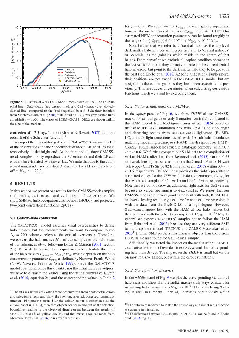
SAM CMASS-mocks 1323

Figure 5. LFs for GALACTICUS’ CMASS-mock samples: Gal-cols (bluesolid line), Gal-dens (red dashed line), and Gal-mass (grey dotted–dashed line) compared to the ‘red sequence’ best fit Schechter functionfrom Montero-Dorta et al. (2016, table 3 and fig. 14) (thin grey dashed line)at redshift z = 0.555. The errors of BOSS-CMASS DR12 are shown withinthe size of the markers.

correction of −2.5 log10(1 + z) (Blanton & Roweis 2007) to fit theredshift of the Schechter function.11

We report that the reddest galaxies of GALACTICUS exceed the LFof the observations and the Schechter-fit of about 0.40 and 0.25 mag,respectively, at the bright end. At the faint end all three CMASS-mock samples poorly reproduce the Schechter-fit and their LF canroughly be estimated by a power law. We note that due to the cut ini-band magnitude (see equation 3) Gal-cols’s LF is abruptly cutoff at MAB ∼ −22.2.

5 R ESULTS

In this section we present our results for the CMASS-mock samplesGal-cols, Gal-mass, and Gal-dens of GALACTICUS. Weshow SHMFs, halo occupation distributions (HODs), and projectedtwo-point correlation functions (2pCFs).

5.1 Galaxy–halo connection

The GALACTICUS model assumes virial overdensities to definehalo masses, but the measurements we want to compare to use%c = 200, where c refers to the critical overdensity. Therefore,we convert the halo masses Mvir of our samples to the halo massof our references M200c following Łokas & Mamon (2001, section2.1). Particularly, we use their equation (8) to calculate the ratioof the halo masses PMHalo = M200c/Mvir which depends on the haloconcentration parameter CNFW as defined by Navarro–Frenk–White(NFW, Navarro, Frenk & White 1997). Since the GALACTICUS

model does not provide this quantity nor the virial radius as outputs,we have to estimate the values using the fitting formula of Klypinet al. (2016, equation 24) and the corresponding values in Table 2

11The fit uses BOSS data which were deconvolved from photometric errorsand selection effects and show the raw, uncorrected, observed luminosityfunction. Photometric errors blur the colour–colour distribution (see themiddle panel in Fig. 3), therefore objects scatter in and out of the selectionboundaries leading to the observed disagreement between the results ofCMASS DR12 (filled yellow circles) and the intrinsic red-sequence fromMontero-Dorta et al. (2016, thin grey dashed line).

for z = 0.50. We calculate the PMHalo for each galaxy separately,however the median over all ratios is PMHalo ∼ 0.884 ± 0.002. Ourestimated NFW concentration parameters can be found roughly inthe range of 4 ! CNFW ! 6 for 1013.3 < M200c < 1015.3 M⊙.

Note further that we refer to a ‘central halo’ as the top-leveldark matter halo in a certain merger tree and to ‘central galaxies’or ‘centrals’ as the galaxies which reside in the centre of thathaloes. From hereafter we exclude all orphan satellites because inthe GALACTICUS model they are not connected to the current centralhalo anymore, but point to the dark matter halo they belonged to inthe past (see Knebe et al. 2018, A2 for clarification). Furthermore,their positions are not traced in the GALACTICUS model, but areassigned to the central galaxies they have been associated to pre-viously. This introduces uncertainties when calculating correlationfunctions which we avoid by excluding them.

5.1.1 Stellar to halo mass ratio M∗/M200c

In the upper panel of Fig. 6, we show SHMF of our CMASS-mocks for central galaxies only (hereafter ‘centrals’) compared tothe HAM model from Rodrıguez-Torres et al. (2016) based onthe BIGMULTIDARK simulation box with 2.5 h−1Gpc side-lengthand clustering results from BOSS–CMASS light-cone [BIGMD-LC, a mock light-cone constructed with the sub-halo abundancematching modelling technique (sHAM) which reproduces BOSS-CMASS DR12 large-scale structure catalogue perfectly] within 0.5< z < 0.6. We further compare our SAM data to a compilation ofvarious HAM realizations from Behroozi et al. (2013)12 at z ∼ 0.55and weak-lensing measurements from the Canada–France–HawaiiTelescope (CFHT) Stripe 82 from Shan et al. (2017) within 0.4 < z

< 0.6, respectively. The additional y-axis on the right represents theestimated values for the NFW profile halo concentration, CNFW, forthe two mock samples, Gal-cols and Gal-dens, respectively.Note that we do not show an additional right axis for Gal-massbecause its values are similar to Gal-cols. We report that ourCMASS-mocks are in very good agreement with both, BIGMD-LCand weak-lensing results e.g. Gal-cols and Gal-mass coincidewith the data from the BIGMD-LC to a high degree. However,Gal-dens agrees best with the HAM at low halo masses butthen coincide with the other two samples at M200c ∼ 1013.5 M⊙. Ingeneral we expect GALACTICUS’ samples not to follow the HAMfrom Behroozi et al. (2013) because they use very different SMFto build-up their model (PRIMUS and GALEX Moustakas et al.201313). Their SMF predicts less massive objects than those fromBOSS as we also found for Gal-dens sample.

Additionally, we tested the impact on the results using GALACTI-CUS native definition of overdensities (%BN98) and their correspond-ing halo mass MBN98. The impact on the SHMF is small but visibleon most massive haloes, but within the error estimations.

5.1.2 Star formation efficiency

In the middle panel of Fig. 6 we plot the corresponding M∗ at fixedhalo mass and show that the stellar masses truly stays constant forincreasing halo masses up to MHalo ∼ 1013.5 M⊙ considering Gal-cols and Gal-mass. Then M∗ increases continuously which

12The data were modified to match the cosmology and initial mass functionwe assume in this paper.13The difference between GALEX and GALACTICUS can be found in Knebeet al. (2018, fig. 1).

MNRAS 486, 1316–1331 (2019)

Dow

nloaded from https://academ

ic.oup.com/m

nras/article-abstract/486/1/1316/5393411 by MTA C

SFK CSI user on 23 Septem

ber 2019

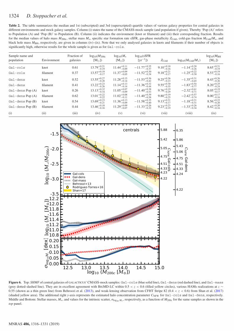
1324 D. Stoppacher et al.

Table 2. The table summarizes the median and 1st (subscripted) and 3rd (superscripted) quartile values of various galaxy properties for central galaxies indifferent environments and mock galaxy samples. Column (i) states the name of the CMASS-mock sample (and population if given). Thereby ‘Pop (A)’ refersto Population (A) and ‘Pop (B)’ to Population (B). Column (ii) indicates the environment (knot or filament) and (iii) their corresponding fraction. Resultsfor the median values of halo mass M200c, stellar mass M∗, specific star formation rate sSFR, gas-phase metallicity ZCold, cold-gas fraction MCold/M∗, andblack hole mass MBH, respectively, are given in columns (iv)–(ix). Note that we only analysed galaxies in knots and filaments if their number of objects issignificantly high, otherwise results for the whole sample is given as for Gal-cols.

Sample name andpopulation Environment

Fraction ofgalaxies

log10(M200c[M⊙])

log10(M∗[M⊙])

log10(sSFR[yr−1]) ZCold log10(MCold/M∗)

log10(MBH[M⊙])

Gal-cols knot 0.61 13.79+0.21−0.19 11.44+0.11

−0.09 −11.77+0.35−0.37 9.10+0.18

−0.16 −1.14+0.20−0.26 8.65+0.21

−0.19

Gal-cols filament 0.37 13.57+0.19−0.17 11.37+0.09

−0.05 −11.52+0.30−0.34 9.18+0.21

−0.17 −1.25+0.22−0.30 8.53+0.19

−0.16

Gal-dens knot 0.52 13.55+0.27−0.28 11.28+0.15

−0.14 −11.53+0.36−0.42 9.25+0.36

−0.23 −1.35+0.31−0.65 8.43+0.26

−0.26

Gal-dens filament 0.41 13.22+0.23−0.26 11.14+0.13

−0.14 −11.36+0.32−0.44 9.55+0.30

−0.35 −1.83+0.54−0.77 8.20+0.25

−0.24

Gal-dens Pop (A) knot 0.26 13.13+0.32−0.34 11.05+0.07

−0.09 −11.40+0.38−0.53 9.76+0.19

−0.29 −2.32+0.61−0.71 8.05+0.19

−0.17

Gal-dens Pop (A) filament 0.62 13.01+0.22−0.22 11.02+0.08

−0.11 −11.40+0.39−0.58 9.80+0.19

−0.25 −2.42+0.57−0.74 8.00+0.17

−0.16

Gal-dens Pop (B) knot 0.54 13.69+0.23−0.21 11.36+0.13

−0.09 −11.58+0.35−0.40 9.13+0.21

−0.17 −1.18+0.21−0.31 8.56+0.22

−0.20

Gal-dens Pop (B) filament 0.44 13.46+0.18−0.16 11.29+0.09

−0.07 −11.33+0.26−0.32 9.23+0.23

−0.19 −1.33+0.26−0.34 8.42+0.20

−0.16

(i) (ii) (iii) (iv) (v) (vi) (vii) (viii) (ix)

Figure 6. Top: SHMF of central galaxies of GALACTICUS’ CMASS-mock samples: Gal-cols (blue solid line), Gal-dens (red dashed line), and Gal-mass(grey dotted–dashed line). They are in excellent agreement with BIGMD-LC within 0.5 < z < 0.6 (filled yellow circles), various HAMs realizations at z ∼0.55 (shown as a thin green line) from Behroozi et al. (2013), and weak-lensing observation from CFHT Stripe 82 (0.4 < z < 0.6) from Shan et al. (2017)(shaded yellow area). The additional right y-axis represents the estimated halo concentration parameter CNFW for Gal-cols and Gal-dens, respectively.Middle and Bottom: Stellar masses, M∗, and values for the intrinsic scatter, σlog10 M∗ , respectively, as a function of M200c for the same samples as shown in thetop panel.

MNRAS 486, 1316–1331 (2019)

Dow

nloaded from https://academ

ic.oup.com/m

nras/article-abstract/486/1/1316/5393411 by MTA C

SFK CSI user on 23 Septem

ber 2019

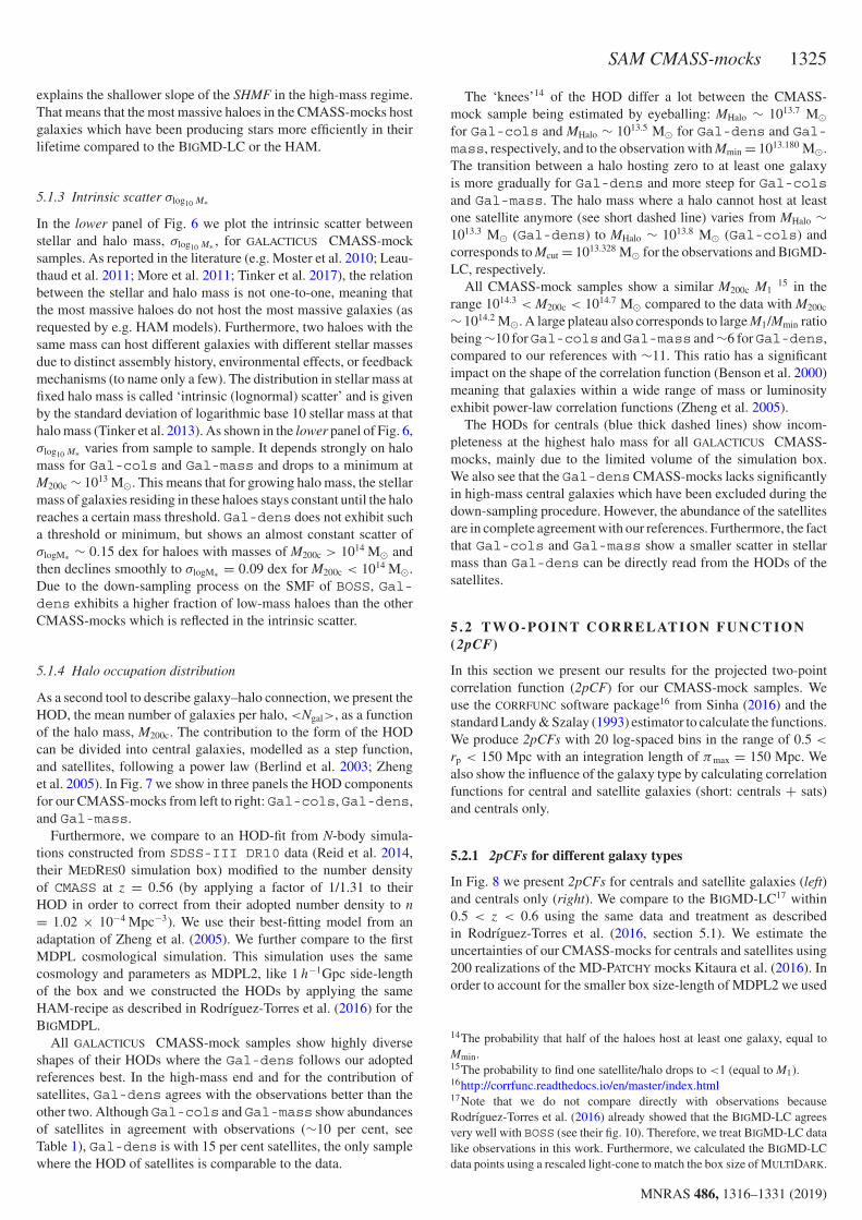
SAM CMASS-mocks 1325

explains the shallower slope of the SHMF in the high-mass regime.That means that the most massive haloes in the CMASS-mocks hostgalaxies which have been producing stars more efficiently in theirlifetime compared to the BIGMD-LC or the HAM.

5.1.3 Intrinsic scatter σlog10 M∗

In the lower panel of Fig. 6 we plot the intrinsic scatter betweenstellar and halo mass, σlog10 M∗ , for GALACTICUS CMASS-mocksamples. As reported in the literature (e.g. Moster et al. 2010; Leau-thaud et al. 2011; More et al. 2011; Tinker et al. 2017), the relationbetween the stellar and halo mass is not one-to-one, meaning thatthe most massive haloes do not host the most massive galaxies (asrequested by e.g. HAM models). Furthermore, two haloes with thesame mass can host different galaxies with different stellar massesdue to distinct assembly history, environmental effects, or feedbackmechanisms (to name only a few). The distribution in stellar mass atfixed halo mass is called ‘intrinsic (lognormal) scatter’ and is givenby the standard deviation of logarithmic base 10 stellar mass at thathalo mass (Tinker et al. 2013). As shown in the lower panel of Fig. 6,σlog10 M∗ varies from sample to sample. It depends strongly on halomass for Gal-cols and Gal-mass and drops to a minimum atM200c ∼ 1013 M⊙. This means that for growing halo mass, the stellarmass of galaxies residing in these haloes stays constant until the haloreaches a certain mass threshold. Gal-dens does not exhibit sucha threshold or minimum, but shows an almost constant scatter ofσlogM∗ ∼ 0.15 dex for haloes with masses of M200c > 1014 M⊙ andthen declines smoothly to σlogM∗ = 0.09 dex for M200c < 1014 M⊙.Due to the down-sampling process on the SMF of BOSS, Gal-dens exhibits a higher fraction of low-mass haloes than the otherCMASS-mocks which is reflected in the intrinsic scatter.

5.1.4 Halo occupation distribution

As a second tool to describe galaxy–halo connection, we present theHOD, the mean number of galaxies per halo, <Ngal>, as a functionof the halo mass, M200c. The contribution to the form of the HODcan be divided into central galaxies, modelled as a step function,and satellites, following a power law (Berlind et al. 2003; Zhenget al. 2005). In Fig. 7 we show in three panels the HOD componentsfor our CMASS-mocks from left to right: Gal-cols, Gal-dens,and Gal-mass.

Furthermore, we compare to an HOD-fit from N-body simula-tions constructed from SDSS-III DR10 data (Reid et al. 2014,their MEDRES0 simulation box) modified to the number densityof CMASS at z = 0.56 (by applying a factor of 1/1.31 to theirHOD in order to correct from their adopted number density to n= 1.02 × 10−4 Mpc−3). We use their best-fitting model from anadaptation of Zheng et al. (2005). We further compare to the firstMDPL cosmological simulation. This simulation uses the samecosmology and parameters as MDPL2, like 1 h−1Gpc side-lengthof the box and we constructed the HODs by applying the sameHAM-recipe as described in Rodrıguez-Torres et al. (2016) for theBIGMDPL.

All GALACTICUS CMASS-mock samples show highly diverseshapes of their HODs where the Gal-dens follows our adoptedreferences best. In the high-mass end and for the contribution ofsatellites, Gal-dens agrees with the observations better than theother two. Although Gal-cols and Gal-mass show abundancesof satellites in agreement with observations (∼10 per cent, seeTable 1), Gal-dens is with 15 per cent satellites, the only samplewhere the HOD of satellites is comparable to the data.

The ‘knees’14 of the HOD differ a lot between the CMASS-mock sample being estimated by eyeballing: MHalo ∼ 1013.7 M⊙for Gal-cols and MHalo ∼ 1013.5 M⊙ for Gal-dens and Gal-mass, respectively, and to the observation with Mmin = 1013.180 M⊙.The transition between a halo hosting zero to at least one galaxyis more gradually for Gal-dens and more steep for Gal-colsand Gal-mass. The halo mass where a halo cannot host at leastone satellite anymore (see short dashed line) varies from MHalo ∼1013.3 M⊙ (Gal-dens) to MHalo ∼ 1013.8 M⊙ (Gal-cols) andcorresponds to Mcut = 1013.328 M⊙ for the observations and BIGMD-LC, respectively.

All CMASS-mock samples show a similar M200c M115 in the

range 1014.3 < M200c < 1014.7 M⊙ compared to the data with M200c

∼ 1014.2 M⊙. A large plateau also corresponds to large M1/Mmin ratiobeing ∼10 forGal-cols andGal-mass and ∼6 forGal-dens,compared to our references with ∼11. This ratio has a significantimpact on the shape of the correlation function (Benson et al. 2000)meaning that galaxies within a wide range of mass or luminosityexhibit power-law correlation functions (Zheng et al. 2005).

The HODs for centrals (blue thick dashed lines) show incom-pleteness at the highest halo mass for all GALACTICUS CMASS-mocks, mainly due to the limited volume of the simulation box.We also see that the Gal-dens CMASS-mocks lacks significantlyin high-mass central galaxies which have been excluded during thedown-sampling procedure. However, the abundance of the satellitesare in complete agreement with our references. Furthermore, the factthat Gal-cols and Gal-mass show a smaller scatter in stellarmass than Gal-dens can be directly read from the HODs of thesatellites.

5 . 2 T WO - P O I N T C O R R E L AT I O N F U N C T I O N(2pCF)

In this section we present our results for the projected two-pointcorrelation function (2pCF) for our CMASS-mock samples. Weuse the CORRFUNC software package16 from Sinha (2016) and thestandard Landy & Szalay (1993) estimator to calculate the functions.We produce 2pCFs with 20 log-spaced bins in the range of 0.5 <

rp < 150 Mpc with an integration length of πmax = 150 Mpc. Wealso show the influence of the galaxy type by calculating correlationfunctions for central and satellite galaxies (short: centrals + sats)and centrals only.

5.2.1 2pCFs for different galaxy types

In Fig. 8 we present 2pCFs for centrals and satellite galaxies (left)and centrals only (right). We compare to the BIGMD-LC17 within0.5 < z < 0.6 using the same data and treatment as describedin Rodrıguez-Torres et al. (2016, section 5.1). We estimate theuncertainties of our CMASS-mocks for centrals and satellites using200 realizations of the MD-PATCHY mocks Kitaura et al. (2016). Inorder to account for the smaller box size-length of MDPL2 we used

14The probability that half of the haloes host at least one galaxy, equal toMmin.15The probability to find one satellite/halo drops to <1 (equal to M1).16http://corrfunc.readthedocs.io/en/master/index.html17Note that we do not compare directly with observations becauseRodrıguez-Torres et al. (2016) already showed that the BIGMD-LC agreesvery well with BOSS (see their fig. 10). Therefore, we treat BIGMD-LC datalike observations in this work. Furthermore, we calculated the BIGMD-LCdata points using a rescaled light-cone to match the box size of MULTIDARK.

MNRAS 486, 1316–1331 (2019)

Dow

nloaded from https://academ

ic.oup.com/m

nras/article-abstract/486/1/1316/5393411 by MTA C

SFK CSI user on 23 Septem

ber 2019

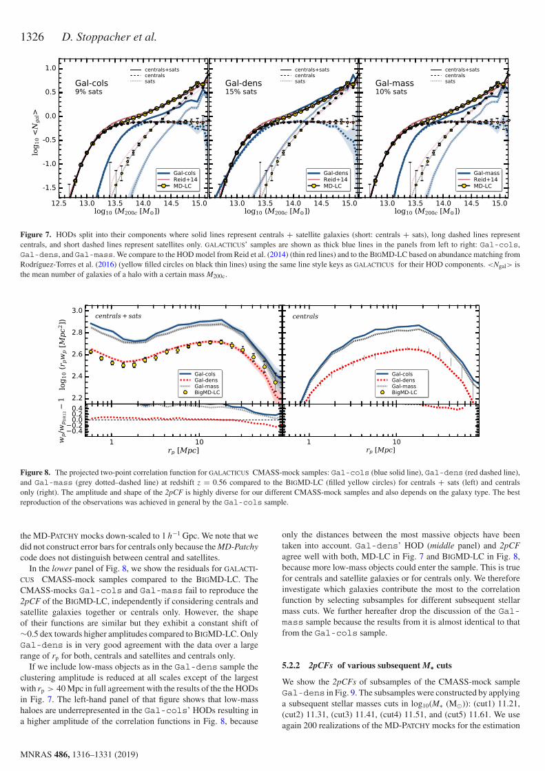
1326 D. Stoppacher et al.

Figure 7. HODs split into their components where solid lines represent centrals + satellite galaxies (short: centrals + sats), long dashed lines representcentrals, and short dashed lines represent satellites only. GALACTICUS’ samples are shown as thick blue lines in the panels from left to right: Gal-cols,Gal-dens, and Gal-mass. We compare to the HOD model from Reid et al. (2014) (thin red lines) and to the BIGMD-LC based on abundance matching fromRodrıguez-Torres et al. (2016) (yellow filled circles on black thin lines) using the same line style keys as GALACTICUS for their HOD components. <Ngal> isthe mean number of galaxies of a halo with a certain mass M200c.

Figure 8. The projected two-point correlation function for GALACTICUS CMASS-mock samples: Gal-cols (blue solid line), Gal-dens (red dashed line),and Gal-mass (grey dotted–dashed line) at redshift z = 0.56 compared to the BIGMD-LC (filled yellow circles) for centrals + sats (left) and centralsonly (right). The amplitude and shape of the 2pCF is highly diverse for our different CMASS-mock samples and also depends on the galaxy type. The bestreproduction of the observations was achieved in general by the Gal-cols sample.

the MD-PATCHY mocks down-scaled to 1 h−1 Gpc. We note that wedid not construct error bars for centrals only because the MD-Patchycode does not distinguish between central and satellites.

In the lower panel of Fig. 8, we show the residuals for GALACTI-CUS CMASS-mock samples compared to the BIGMD-LC. TheCMASS-mocks Gal-cols and Gal-mass fail to reproduce the2pCF of the BIGMD-LC, independently if considering centrals andsatellite galaxies together or centrals only. However, the shapeof their functions are similar but they exhibit a constant shift of∼0.5 dex towards higher amplitudes compared to BIGMD-LC. OnlyGal-dens is in very good agreement with the data over a largerange of rp for both, centrals and satellites and centrals only.

If we include low-mass objects as in the Gal-dens sample theclustering amplitude is reduced at all scales except of the largestwith rp > 40 Mpc in full agreement with the results of the the HODsin Fig. 7. The left-hand panel of that figure shows that low-masshaloes are underrepresented in the Gal-cols’ HODs resulting ina higher amplitude of the correlation functions in Fig. 8, because

only the distances between the most massive objects have beentaken into account. Gal-dens’ HOD (middle panel) and 2pCFagree well with both, MD-LC in Fig. 7 and BIGMD-LC in Fig. 8,because more low-mass objects could enter the sample. This is truefor centrals and satellite galaxies or for centrals only. We thereforeinvestigate which galaxies contribute the most to the correlationfunction by selecting subsamples for different subsequent stellarmass cuts. We further hereafter drop the discussion of the Gal-mass sample because the results from it is almost identical to thatfrom the Gal-cols sample.

5.2.2 2pCFs of various subsequent M∗ cuts

We show the 2pCFs of subsamples of the CMASS-mock sampleGal-dens in Fig. 9. The subsamples were constructed by applyinga subsequent stellar masses cuts in log10(M∗ (M⊙)): (cut1) 11.21,(cut2) 11.31, (cut3) 11.41, (cut4) 11.51, and (cut5) 11.61. We useagain 200 realizations of the MD-PATCHY mocks for the estimation

MNRAS 486, 1316–1331 (2019)

Dow

nloaded from https://academ

ic.oup.com/m

nras/article-abstract/486/1/1316/5393411 by MTA C

SFK CSI user on 23 Septem

ber 2019

SAM CMASS-mocks 1327

Figure 9. Projected two-point correlation functions of subsamples ofGALACTICUS’ CMASS-mock Gal-dens (solid lines) using the subsequentM∗ cuts (indicated by the keys) compared to BOSS-CMASS DR12 (mark-ers).

of the uncertainties as in Fig. 8. Note that we only present results forGal-dens because only this sample provides a sufficient numberdensity of galaxies. We can see in the figure that modelled andobserved galaxies are in poor agreement with each other. In orderto improve the clustering we tried to fix the number density n ofGALACTICUS’ subsamples in order to match those of BOSS-CMASSDR12. This experiment only improved the 2pCF slightly.

6 D ISCUSSION

Before we discuss our results we want to add a few notes about theinfluence of GALACTICUS native tuning and model configuration.Most importantly, GALACTICUS has not been specifically calibratedon MDPL2, but its most favourable parameter set and configurationwere used. Although GALACTICUS was tuned to match the K-, bj-band LFs at z = 0 and the local CMD at z = 0.1, its luminositiesand colours do not perfectly match the CMASS galaxy properties.Therefore, we examine if alternative approaches to select a CMASS-mock (e.g. a cut in stellar mass) would be a convenient approachto bypass this problem. In general the Gal-cols and Gal-masssamples agree very well with each other (see Fig. 3 or results ofSMF, SHMF, HOD, or 2pCF), but both exhibit too low numberdensities compared to CMASS and do not reproduce the 2pCF asshown in Fig. 8.

Why does a density-selected sample work better? First, Gal-dens exhibits by construction the same number density as CMASS.Secondly, although Gal-dens’ galaxies are 1.5–2 mag fainter inthe i-band than Gal-cols, Gal-mass, and CMASS (as shown inthe upper panel of Fig. 3), their stellar masses are fully comparable18

and should have satisfied the CMASS colour–magnitude selectioncriteria, but due to their lower brightness they did not enter thesample selection.

What are the properties of Gal-dens galaxies? We can divideGal-dens into two distinct populations (A) and (B) using a sliding

18Gal-dens is located within the 95 per cent confidence level contour ofCMASS in the (g − i) colour plane as shown in the lower panel of Fig. 3.

Figure 10. Relation between gas-phase metallicity ZCold and sSFR forcentral galaxies of the Gal-cols sample (filled coloured contours) andthe Gal-dens sample (red dashed contours) at z = 0.56.

cut in SFR depending on sSFR.19 Population (A) galaxies are lowstar forming (SFR ∼ 0.05 M⊙yr−1) and live in low-mass haloes(M200c < 1013.3 M⊙) while Population (B) are star forming (0.1 <

SFR < 0.3 M⊙yr−1) residing in most massive haloes (M200c > 1013.3

M⊙). We find a strong dependency on halo mass at fixed sSFRwhere low-mass haloes have a linear relation between SFR andsSFR, while the high-mass haloes exhibit larger SFRs at fixed sSFR.Furthermore, certain galaxy properties related to star formation canbe clearly mapped on to Population (A) or (B) but other propertiessuch as M∗ or (r − i) colour are continuously distributed. Thistrend is particularly interesting because it shows the importance ofsecondary parameters related to the clustering besides halo mass assuggested by Wang, De Lucia & Weinmann (2013).

How do gas-phase properties divide the sample into two distinctpopulations? In Fig. 10 we show the gas-phase metallicity ZCold,20 aproxy for gas-cooling and star formation (Lebouteiller et al. 2013),for central galaxies. The two populations (A) and (B) are reflected inthe bimodal distribution of ZCold where ∼80 per cent of Population(A) shows ZCold > 9.5 and only 20 per cent lower values withZCold ∼ 9.5. The opposite is true for Population (B). Commonstudies of fundamental relations between metallicity, mass, andstar formation suggest that less/more massive galaxies have alsolower/higher metal abundances (Lara-Lopez et al. 2009; Yates et al.

19The following conditional equation divides the sample into Population(A) and (B):

log10(SFR[M⊙ yr−1])!

<δ Pop(A)>δ Pop(B)

where δ = log10(sSFR(yr−1)) + 11.161.12

(13)

20ZCold = 8.69 + log10(MZ,Cold/MCold) − log10(Z⊙), where MZ,Cold is themass of metals in the cold gas-phase. ZCold is normalized by the metallicityof the Sun Z⊙ = 0.0134 (Asplund et al. 2009), while the factor 8.69 (AllendePrieto, Lambert & Asplund 2001) corresponds to its oxygen abundance.

MNRAS 486, 1316–1331 (2019)

Dow

nloaded from https://academ

ic.oup.com/m

nras/article-abstract/486/1/1316/5393411 by MTA C

SFK CSI user on 23 Septem

ber 2019

1328 D. Stoppacher et al.

2012). Our results show that Population (B)’s galaxies are moremassive but have lower metal abundances. This ‘turnover’ was alsoreported by Yates et al. (2012) for modelled galaxies at z = 0and is possibly linked to the infall of metal-poor gas after a gas-rich merger. In Yates & Kauffmann (2014) the same authors studiedmassive galaxies and divide them into an ‘enriching’ and a ‘diluting’sample, the later show similar trends as our Population (B): lowsSFR, lower ZCold, and higher MBH. Furthermore, our findings are intotal agreement with Lara-Lopez et al. (2013) showing that galaxieswith low sSFR have high/low values of ZCold when MCold is low/high.We emphasize that the distinct separation of the two populationscould give clues about galaxy evolution in the context of the originof the fundamental luminosity/mass–metallicity relation, merger-induced star formation, or ‘downsizing’ (Mannucci et al. 2010, seetheir section 1 for comparison).

How do the Populations (A) and (B) relate to environment? Weexpect that Population (A) fixes the clustering amplitude due to theirenvironment as well as their number density. To this extent we applythe VWEB method (see Appendix A for details) to the underlyingdark matter MDPL2 simulation. We show in the second column ofTable 2 that more galaxies in the Gal-cols sample (61 per cent)are assigned into knots than in the Gal-dens sample (52 per cent).We detect a clear environmental dependency of this sample wherePopulations (A) is dominated by filament galaxies (62 per cent withonly 26 per cent in knots), while Population (B) has more galaxiesin the knots (54 per cent) than in the filaments (44 per cent).

Do galaxy properties have a dependency on environment?Besides the number fraction of galaxies, we further detail thesample properties in different environments in Table 2. Galaxiesin filaments generally tend to have lower halo, stellar, and blackhole masses as well as sSFR and cold-gas fraction compared to theones (from the same sample) in knots, while the cold-gas metallicityis normally higher in filaments than in knots. It is worth noting thatPopulation (A) has significantly smaller halo mass, stellar mass,cold-gas fraction, and black hole mass than Population (B) in bothenvironments, but significantly higher cold-gas metallicity in (A)than in (B).

What conclusion can we draw from the environmental depen-dency of galaxy properties? The star formation is not sufficientlysuppressed in Population (B) and the most massive galaxies whichshould be ‘red-and-dead’ are still star forming at a low rate.Therefore, GALACTICUS shows a higher abundance in the high-mass end of the SMF compared to the observed CMASS galaxysample. Furthermore, most of the low-SFR galaxies in the Gal-dens sample live in the filaments in Population (A) with relativelylower MBH and MCold. They are located in haloes with suppressedstar formation and could not grow in mass enough to exhibitbrighter luminosities. This scenario is supported by the fact thatPopulation (A) of Gal-dens has small contents of cold gasand as smaller cold-gas fractions in both knots and filaments,compared to Population (B). We cannot explicitly say why MCold issignificantly smaller but it would imply that the quenching processin GALACTICUS is mostly dominated by tidal stripping of the cold gasinstead of AGN feedback. We find it further interesting that half ofthe galaxies of this population exhibit higher gas-phase metallicities.We could speculate that the two populations (A) and (B) mighthave formed at different times and evolved differently due to theirenvironment (see ‘environmental quenching’ of star formation e.g.Tomczak et al. 2018) or halo masses (see ‘halo quenching’ of low-mass central galaxies e.g. Tal et al. 2014). Different evolutionarypaths (as Montero-Dorta et al. 2017b have shown for BOSS) mighthave contributed to the variations in the intrinsic scatter and could

also provide a signal of the assembly bias, however, further studiesare required to provide proof of that hypothesis.

How is the environmental dependency reflected in the clustering?We expect that the different quenching processes have a crucialimpact on the intrinsic scatter in stellar mass at fixed halo mass,σlog10 M∗ , which in return has an impact on the clustering amplitude.Compared to other works we report that the values of the intrinsicscatter of Gal-cols and Gal-mass with 0.1 dex and Gal-dens with 0.15 dex depending on the halo mass. Those resultsare similar to Rodrıguez-Torres et al. (2016), who found a scatterof 0.14 dex for their CMASS abundance matching BIGMD-LC.However, Shankar et al. (2014) stated that an intrinsic scatter of atleast 0.15 dex is needed to reproduce the BOSS clustering whichmeans that GALACTICUS in general shows an insufficient levelof scatter. Furthermore, Tinker et al. (2017) reported a slightlylarger observed scatter of σlogM∗ = 0.18+0.01

−0.02 dex for CMASS andLeauthaud et al. (2012) of 0.249 ± 0.019 dex measured from passivegalaxies in the COSMOS survey (Scoville et al. 2007). Gu, Conroy& Behroozi (2016) found similar values for the intrinsic scatterσlogM∗ < 0.2 and emphasize that the origin of the scatter in theSHMF at higher masses is induced by the hierarchical assembly,while at low halo masses it is associated with in situ growth. Smallerscatter could mean that there is insufficient scatter in the assemblyhistories, or that the galaxy formation models do not capture all ofit. However, understanding this issue is a non-trivial task and onehas to address model specific properties in more detail to understandwhich combination of properties causes this effect. We find that thecomparison with other SAMs would help on this task, but wouldbe beyond the scope of this paper and is therefore left for furtherstudies.

7 SU M M A RY

Our work is based on the BOSS (Schlegel et al. 2009; Dawson et al.2013) of the Sloan Digital Sky Survey (SDSS-III, Eisenstein et al.2011) CMASS (for ‘constant mass’) sample and a semi-analyticalmodel of galaxy formation (SAM), called GALACTICUS, as part of theMULTIDARK-GALAXIES products (Knebe et al. 2018). The CMASSsample was build from the SDSS-III/BOSS survey catalogues byapplying a complex colour–magnitude selection (see equations 1–4). We use the same selection scheme to extract our modelled galaxycatalogue from GALACTICUS, called Gal-cols, at z = 0.56.

We provide detail assessment of the SAM via comparing withBOSS as well as results on the galaxy–halo connection and cluster-ing studies of the two-point correlation function. For reasons statedin Section 3, we construct two additional CMASS-mock samples.The first one is called Gal-dens and was build by randomlyselecting modelled galaxies (or down-sampling) until they fit theobservational SMF of BOSS in the range 0.5 < z < 0.6. Thesecond CMASS-mock is called Gal-mass and was generated byapplying a high stellar mass cut of M∗ > 1011.24 M⊙ as introducedby Maraston et al. (2013). Here we summarize major results of ourstudy.

(i) The GALACTICUS colour–magnitude-selected CMASS-mocksample, Gal-cols, shows a lower number density, fewer blueobjects, and is located within a smaller parameter space comparedto the observational sample (see Fig. 1). Its RS is intrinsicallyconcentrated, as predicted by Montero-Dorta et al. (2016) (seeFig. 2). Although the number density of this sample is only 1/3 thedensity of BOSS galaxies, Gal-cols overpredicts red galaxiesat M∗ " 1012 M⊙ (see Fig. 4). Galaxies in Gal-dens satisfy the

MNRAS 486, 1316–1331 (2019)

Dow

nloaded from https://academ

ic.oup.com/m

nras/article-abstract/486/1/1316/5393411 by MTA C

SFK CSI user on 23 Septem

ber 2019

SAM CMASS-mocks 1329

CMASS colour selection criteria, but they did not enter the sampleselection due to their luminosities being approximately 1.5–2 maglower in i-band (see the middle panel of Fig. 3).

(ii) GALACTICUS Gal-cols and Gal-mass samples agreevery well with the stellar to halo mass relation of Rodrıguez-Torreset al. (2016) and weak-lensing results from Shan et al. (2017),while Gal-dens shows similar behaviour as the HAM modelfrom Behroozi et al. (2013) (see Fig. 6). However, all three CMASS-mock samples exhibit an increasing scatter at fixed halo mass fromσlogM∗ ∼ 0.05–0.15 dex depending on halo mass. Compared to otherworks with σlogM∗ = 0.14 dex by Rodrıguez-Torres et al. (2016),σlogM∗ = 0.18+0.01

−0.02 dex by Tinker et al. (2017), or 0.249 ± 0.019 dexby Leauthaud et al. (2012), GALACTICUS displays an insufficientlevel of scatter.

(iii) Gal-cols and Gal-mass agree poorly with the cluster-ing of CMASS galaxies from the high-fidelity mock BIGMD-LC(Rodrıguez-Torres et al. 2016), which was obtained using HAMtechniques. We find that the combination of low intrinsic scatterat fixed halo mass and missing objects (or objects being too faint)is responsible for the high clustering amplitudes of Gal-colsand Gal-mass. However, the Gal-dens sample reproduces theclustering of central and satellite galaxies as well as of centrals only,within 1σ (see Fig. 8).

(iv) We can divide the Gal-cols and Gal-dens samplesinto two subpopulations, (A) and (B), using a given SFR cut.Population (A) corresponds to low star-forming galaxies in lowermass haloes, while Population (B) is comprised of mildly star-forming galaxies living in the most massive haloes. (A)-galaxieswere found as the population which displays too faint luminositiesas mentioned in (i), but fix the clustering amplitude due to theenvironmental affiliation and number density. Using the VWEB code(see Appendix A) we confirm that (A)-galaxies live in filaments,while (B)-galaxies can be found in knots.

(v) We find further correlations between halo mass M200c andstar-formation-related properties as (specific) star formation rate,gas-phase metallicity, Zcold, and cold-gas fraction, MCold/M∗, butalso black hole mass MBH, depending on the environment andsubpopulation (A) and (B) where e.g. 80 per cent of galaxies inPopulation (A) show higher sSFR and Zcold > 9.5, but lower cold-gas fractions and black hole masses compared to their counterpartsin Population (B) (see Table 2).

In this work, we have carefully examined several samples of themost massive galaxies from the GALACTICUS galaxy formationmodel. In a follow-up work, we plan to extend this analysis to otherSAMs in order to study in more detail the star formation historyof massive galaxies at intermediate redshifts. This follow-up studywill be connected to the effect of galaxy assembly bias, a crucialaspect to the formation and evolution of galaxies.

ACKNOWLEDGEMENTS

DS, FP, ADMD, SRT, GF, and AAK want to thank the support ofthe Spanish Ministry grant AYA2014-60641-C2-1-P managed bythe Instituto de Astrofısica de Andalucıa (IAA-CSIC).

WC and AK are supported by the Ministerio de Economıa yCompetitividad and the Fondo Europeo de Desarrollo Regional(MINECO/FEDER, UE) in Spain through grant AYA2015-63810-P.

WC further acknowledges the supported by the European Re-search Council under grant number 670193.

AK is also supported by the Spanish Red Consolider Multi-Dark FPA2017-90566-REDC. He further thanks Lance Jyo fordreamwalking.

ADMD thanks Fundacao de Amparo a Pesquisa do Estado deSao Paulo (FAPESP) for financial support.

DS fellowship is funded by the Spanish Ministry of Economyand Competitiveness (MINECO) under the 2014 Severo OchoaPredoctoral Training Programme. The author also wants to thankthe Bocono Specialty Coffee-team for their kind supply of energy.

This work was created using the following software prod-ucts and collaborative online platforms: OVERLEAF,21 CENTOS6,22 MATPLOTLIB23 2012–2016, Hunter (2007); PYTHON SOFT-WARE FOUNDATION24 1990–2017, version 2.7, PYTHONBREW25;COSMOLOPY26; we use whenever possible in this work a colour-blind friendly colour palette27 for our figures.

The CosmoSim data base used in this paper is a service by theLeibniz-Institute for Astrophysics Potsdam (AIP). We want to thankthe AIP and the server admin team for using their computationalfacilities and their support.

This research has used NASA’s Astrophysics Data System (ADS)and the arXiv preprint server.

We also want to thank the anonymous reviewer for their carefulreading of our manuscript and their many insightful comments andsuggestions that improved significantly this publication.

R E F E RENCES

Alam S. et al., 2015, ApJS, 219, 12Alam S. et al.., 2017, MNRAS, 470, 2617Allende Prieto C., Lambert D. L., Asplund M., 2001, ApJ, 556, L63Almeida C., Baugh C. M., Wake D. A., Lacey C. G., Benson A. J., Bower

R. G., Pimbblet K., 2008, MNRAS, 386, 2145Anderson L. et al., 2014, MNRAS, 441, 24Asplund M., Grevesse N., Sauval A. J., Scott P., 2009, ARA&A, 47, 481Baugh C. M., 2006, Rep. Prog. Phys., 69, 3101Baugh C. M., 2013, in The Intriguing Life of Massive Galaxies, IAU

Symposium, Vol 295. p. 191Behroozi P. S., Wechsler R. H., Conroy C., 2013, ApJ, 770, 57Behroozi P. S., Wechsler R. H., Wu H.-Y., 2013a, ApJ, 762, 109Behroozi P. S., Wechsler R. H., Wu H.-Y., Busha M. T., Klypin A. A.,

Primack J. R., 2013b, ApJ, 763, 18Benson A. J., 2010, Phys. Rep., 495, 33Benson A. J., 2012, New Astron., 17, 175Benson A. J., Cole S., Frenk C. S., Baugh C. M., Lacey C. G., 2000, MNRAS,

311, 793Benson A. J., Bower R. G., Frenk C. S., Lacey C. G., Baugh C. M., Cole S.,

2003, ApJ, 599, 38Berlind A. A. et al., 2003, ApJ, 593, 1Bernardi M., Meert A., Sheth R. K., Huertas-Company M., Maraston C.,

Shankar F., Vikram V., 2016, MNRAS, 455, 4122Beutler F. et al., 2014, MNRAS, 444, 3501Blanton M. R., Roweis S., 2007, AJ, 133, 734Bower R. G., Benson A. J., Malbon R., Helly J. C., Frenk C. S., Baugh C.

M., Cole S., Lacey C. G., 2006, MNRAS, 370, 645Bryan G. L., Norman M. L., 1998, ApJ, 495, 80Campbell D. J. R. et al., 2015, MNRAS, 452, 852

21www.overleaf.com22http://www.centos.org/23http://matplotlib.org/24http://www.python.org25https://github.com/utahta/pythonbrew26http://roban.github.io/CosmoloPy/docAPI/cosmolopy-module.html27https://personal.sron.nl/ pault/

MNRAS 486, 1316–1331 (2019)

Dow

nloaded from https://academ

ic.oup.com/m

nras/article-abstract/486/1/1316/5393411 by MTA C

SFK CSI user on 23 Septem

ber 2019

1330 D. Stoppacher et al.

Cannon R. et al., 2006, MNRAS, 372, 425Carlesi E., Knebe A., Lewis G. F., Wales S., Yepes G., 2014, MNRAS, 439,

2943Chabrier G., 2003, PASP, 115, 763Chuang C.-H. et al., 2016, MNRAS, 461, 3781Collacchioni F., Cora S. A., Lagos C. D. P., Vega-Martınez C. A., 2018,

MNRAS, 481, 954Conroy C., Gunn J. E., White M., 2009, ApJ, 699, 486Contreras S., Baugh C. M., Norberg P., Padilla N., 2013, MNRAS, 432,

2717Contreras S., Baugh C. M., Norberg P., Padilla N., 2015, MNRAS, 452,

1861Cora S. A., 2016, Bol. Asociacion Argentina Astron. La Plata Argentina,

58, 8Cora S. A., Hough T., Vega-Martınez C. A., Orsi A. A., 2019, MNRAS,

483, 1686,Cuesta A. J. et al., 2016, MNRAS, 457, 1770Cui W. et al., 2019, MNRAS, 485, 2367Cui W., Knebe A., Yepes G., Yang X., Borgani S., Kang X., Power C.,

Staveley-Smith L., 2018, MNRAS, 473, 68Dawson K. S. et al., 2013, AJ, 145, 10Eisenstein D. J. et al., 2001, AJ, 122, 2267Eisenstein D. J. et al., 2011, AJ, 142, 72Farrow D. J. et al., 2015, MNRAS, 454, 2120Favole G., McBride C. K., Eisenstein D. J., Prada F., Swanson M. E., Chuang

C.-H., Schneider D. P., 2016, MNRAS, 462, 2218Ferrara A., Bianchi S., Cimatti A., Giovanardi C., 1999, ApJS, 123, 437Fukugita M., Ichikawa T., Gunn J. E., Doi M., Shimasaku K., Schneider D.

P., 1996, AJ, 111, 1748Gil-Marın H., Percival W. J., Verde L., Brownstein J. R., Chuang C.-H.,

Kitaura F.-S., Rodrıguez-Torres S. A., Olmstead M. D., 2017, MNRAS,465, 1757

Gonzalez-Perez V., Lacey C. G., Baugh C. M., Lagos C. D. P., Helly J.,Campbell D. J. R., Mitchell P. D., 2014, MNRAS, 439, 264

Gruppioni C. et al., 2015, MNRAS, 451, 3419Gu M., Conroy C., Behroozi P., 2016, ApJ, 833, 2Guo H. et al., 2014, MNRAS, 441, 2398Guo H. et al., 2013, ApJ, 767, 122Guo H., Yang X., Lu Y., 2018, ApJ, 858, 30Henriques B. M. B., White S. D. M., Lilly S. J., Bell E. F., Bluck A. F. L.,

Terrazas B. A., 2019, MNRAS, 485, 3446Henriques B. M. B., White S. D. M., Thomas P. A., Angulo R. E., Guo Q.,

Lemson G., Wang W., 2017, MNRAS, 469, 2626Hoffman Y., Metuki O., Yepes G., Gottlober S., Forero-Romero J. E.,

Libeskind N. I., Knebe A., 2012, MNRAS, 425, 2049Hunter J. D., 2007, Comput. Sci. Eng., 9, 90Kitaura F.-S. et al., 2016, MNRAS, 456, 4156Klypin A., Yepes G., Gottlober S., Prada F., Heß S., 2016, MNRAS, 457,

4340Knebe A. et al., 2018, MNRAS, 474, 5206Kroupa P., 2001, MNRAS, 322, 231Lacey C. G. et al., 2016, MNRAS, 462, 3854Lagos C. D. P., Baugh C. M., Zwaan M. A., Lacey C. G., Gonzalez-Perez

V., Power C., Swinbank A. M., van Kampen E., 2014, MNRAS, 440,920

Landy S. D., Szalay A. S., 1993, ApJ, 412, 64Lara-Lopez M. A. et al., 2013, MNRAS, 433, L35Lara-Lopez M. A., Cepa J., Bongiovanni A., Perez Garcıa A. M., Casta neda

H., Fernandez Lorenzo M., Povic M., Sanchez-Portal M., 2009, A&A,505, 529

Leauthaud A., Tinker J., Behroozi P. S., Busha M. T., Wechsler R. H., 2011,ApJ, 738, 45

Leauthaud A. et al., 2012, ApJ, 744, 159Lebouteiller V., Heap S., Hubeny I., Kunth D., 2013, A&A, 553, A16Libeskind N. I., Hoffman Y., Knebe A., Steinmetz M., Gottlober S., Metuki

O., Yepes G., 2012, MNRAS, 421, L137Libeskind N. I., Hoffman Y., Forero-Romero J., Gottlober S., Knebe A.,

Steinmetz M., Klypin A., 2013, MNRAS, 428, 2489

Lietzen H., Tempel E., Heinamaki P., Nurmi P., Einasto M., Saar E., 2012,A&A, 545, A104

Liu G. C., Lu Y. J., Xie L. Z., Chen X. L., Zhao Y. H., 2016, A&A, 585,A52

Łokas E. L., Mamon G. A., 2001, MNRAS, 321, 155Mannucci F., Cresci G., Maiolino R., Marconi A., Gnerucci A., 2010,

MNRAS, 408, 2115Maraston C. et al., 2013, MNRAS, 435, 2764Maraston C., 2005, MNRAS, 362, 799Maraston C., Daddi E., Renzini A., Cimatti A., Dickinson M., Papovich C.,

Pasquali A., Pirzkal N., 2006, ApJ, 652, 85Maraston C., Stromback G., Thomas D., Wake D. A., Nichol R. C., 2009,

MNRAS, 394, L107Masters K. L. et al., 2011, MNRAS, 418, 1055Montero-Dorta A. D., Bolton A. S., Shu Y., 2017a, MNRAS, 468, 47Montero-Dorta A. D. et al., 2016, MNRAS, 461, 1131Montero-Dorta A. D. et al., 2017b, ApJ, 848, L2More S., van den Bosch F. C., Cacciato M., Skibba R., Mo H. J., Yang X.,

2011, MNRAS, 410, 210Moster B. P., Somerville R. S., Maulbetsch C., van den Bosch F. C., Maccio

A. V., Naab T., Oser L., 2010, ApJ, 710, 903Moustakas J. et al., 2013, ApJ, 767, 50Mueller E.-M., Percival W., Linder E., Alam S., Zhao G.-B., Sanchez A. G.,

Beutler F., Brinkmann J., 2018, MNRAS, 475, 2122Mutch S. J., Poole G. B., Croton D. J., 2013, MNRAS, 428, 2001Navarro J. F., Frenk C. S., White S. D. M., 1997, ApJ, 490, 493Nuza S. E. et al., 2013, MNRAS, 432, 743Orsi A., Padilla N., Groves B., Cora S., Tecce T., Gargiulo I., Ruiz A., 2014,

MNRAS, 443, 799Planck Collaboration, 2015, A&A, 594, A13Reid B. et al., 2016, MNRAS, 455, 1553Reid B. A., Seo H.-J., Leauthaud A., Tinker J. L., White M., 2014, MNRAS,

444, 476Ren K., Trenti M., Mutch S. J., 2018, ApJ, 856, 81Rodrigues L. F. S., Vernon I., Bower R. G., 2017, MNRAS, 466, 2418Rodrıguez-Torres S. A. et al., 2016, MNRAS, 460, 1173Ross A. J. et al., 2017, MNRAS, 472, 4456Saito S. et al., 2016, MNRAS, 460, 1457Schlegel D., White M., Eisenstein D., 2009, in astro2010: The Astronomy

and Astrophysics Decadal Survey. preprint (arXiv:0902.4680)Scoville N. et al., 2007, ApJS, 172, 1Shan H. et al., 2017, ApJ, 840, 104Shankar F. et al., 2014, MNRAS, 439, 3189Shirakata H. et al., 2019, MNRAS, 482, 4846Sinha M., 2016, Corrfunc: Corrfunc-1.1.0.Somerville R. S., Dave R., 2015, ARA&A, 53, 51Springel V. et al., 2005, Nature, 435, 629Sullivan J. M., Wiegand A., Eisenstein D. J., 2017, preprint (arXiv:1711.0

9899)Tal T. et al., 2014, ApJ, 789, 164Tinker J. L. et al., 2017, ApJ, 839, 121Tinker J. L., Leauthaud A., Bundy K., George M. R., Behroozi P., Massey

R., Rhodes J., Wechsler R. H., 2013, ApJ, 778, 93Tomczak A. R. et al., 2018, MNRAS, 484, 4695van Daalen M. P., Henriques B. M. B., Angulo R. E., White S. D. M., 2016,

MNRAS, 458, 934Wang L., De Lucia G., Weinmann S. M., 2013, MNRAS, 431, 600Wechsler R. H., Tinker J. L., 2018, ARA&A, 56, 435White M. et al., 2011, ApJ, 728, 126White S. D. M., Frenk C. S., 1991, ApJ, 379, 52Xie L., De Lucia G., Hirschmann M., Fontanot F., Zoldan A., 2017, MNRAS,

469, 968Yates R. M., Kauffmann G., 2014, MNRAS, 439, 3817Yates R. M., Kauffmann G., Guo Q., 2012, MNRAS, 422, 215Zheng Z. et al., 2005, ApJ, 633, 791Zoldan A., De Lucia G., Xie L., Fontanot F., Hirschmann M., 2018, MNRAS,

481, 1376

MNRAS 486, 1316–1331 (2019)

Dow

nloaded from https://academ

ic.oup.com/m

nras/article-abstract/486/1/1316/5393411 by MTA C

SFK CSI user on 23 Septem

ber 2019

SAM CMASS-mocks 1331

A P P E N D I X A : T H E V W E B M E T H O D

This Vweb method applies the shear tensor technique classify thelarge-scale environments into either ‘void’, ‘sheet’, ‘filament’, or‘knot’. Following Hoffman et al. (2012), the velocity shear tensoris defined as

*αβ = − 12H0

!∂vα

∂rβ

+ ∂vβ

∂rα

", (A1)

where, H0 is the Hubble constant. The eigenvalues of *αβ aredenoted as λi (i = 1, 2 and 3).

The simulation box is separated into cubic mesh cells, withinwhich the velocity field is calculated. Each cell has a size of ∼1 Mpc.After smoothing the velocity field, we calculate the eigenvalues ofthe velocity shear tensor in each cell. Each cell is then classifiedas either ‘void’, ‘sheet’, ‘filament’, or ‘knot’ according to theeigenvalues λ1 > λ2 > λ3:

(1) void, if λ1 < λth,(2) sheet, if λ1 ≥ λth > λ2,(3) filament, if λ2 ≥ λth > λ3,(4) knot, if λ3 ≥ λth,

where λth is a free threshold parameter (Hoffman et al. 2012;Libeskind et al. 2012, 2013). Following the discussion of Carlesiet al. (2014); Cui et al. (2018, 2019), we set λth = 0.1, whichpresents better agreement to the visualized density field. Our mockgalaxies are then placed on to the same grid checking for the webclassification of the cell they lie in.

This paper has been typeset from a TEX/LATEX file prepared by the author.

MNRAS 486, 1316–1331 (2019)

Dow

nloaded from https://academ

ic.oup.com/m

nras/article-abstract/486/1/1316/5393411 by MTA C

SFK CSI user on 23 Septem

ber 2019

5 Paper III – The Three HundredClusters

Publication

Title: The Three Hundred project: a large catalogue of theoretically modelledgalaxy clusters for cosmological and astrophysical applications

Reference: Monthly Notices of the Royal Astronomical Society, Volume 480, Issue3, p.2898-2915

Date: November 2018

Motivation

The large-scale distribution of galaxies in the Universe is dominated by the endeavour of galaxiesto group into clusters and superclusters. Galaxy clusters are the largest gravitationally boundobjects and therefore consist of excellent laboratories to study galaxy formation and evolution[159]. The formation of clusters depends, on the one hand, on the underlying cosmological frame-work, but on the other hand, on various complex physical processes and feedback mechanismsregulating and shaping galaxy properties. Those processes and properties are tightly correlatedwith each other and depend on their underlying dark matter distribution as well as their largeand small-scale environments [51, 181, 256, 272], which makes it difficult to fully entangle them.Since we are particularly interested in studying luminous red galaxies (as introduced in Chap-ter 4) and what shapes their galaxy properties, The Three Hundred project provides aperfect baseline for such an effort. The project includes more than 300 simulated cluster regionsusing various modelling techniques such flavours of full-hydrodynamical simulations and the,in Chapter 3 introduced, The MultiDark-Galaxies semi-analytical models. In whatfollows, we will study the properties of the clusters and their associated galaxies in detail as wellas present a comparison on the different modelling techniques.

73

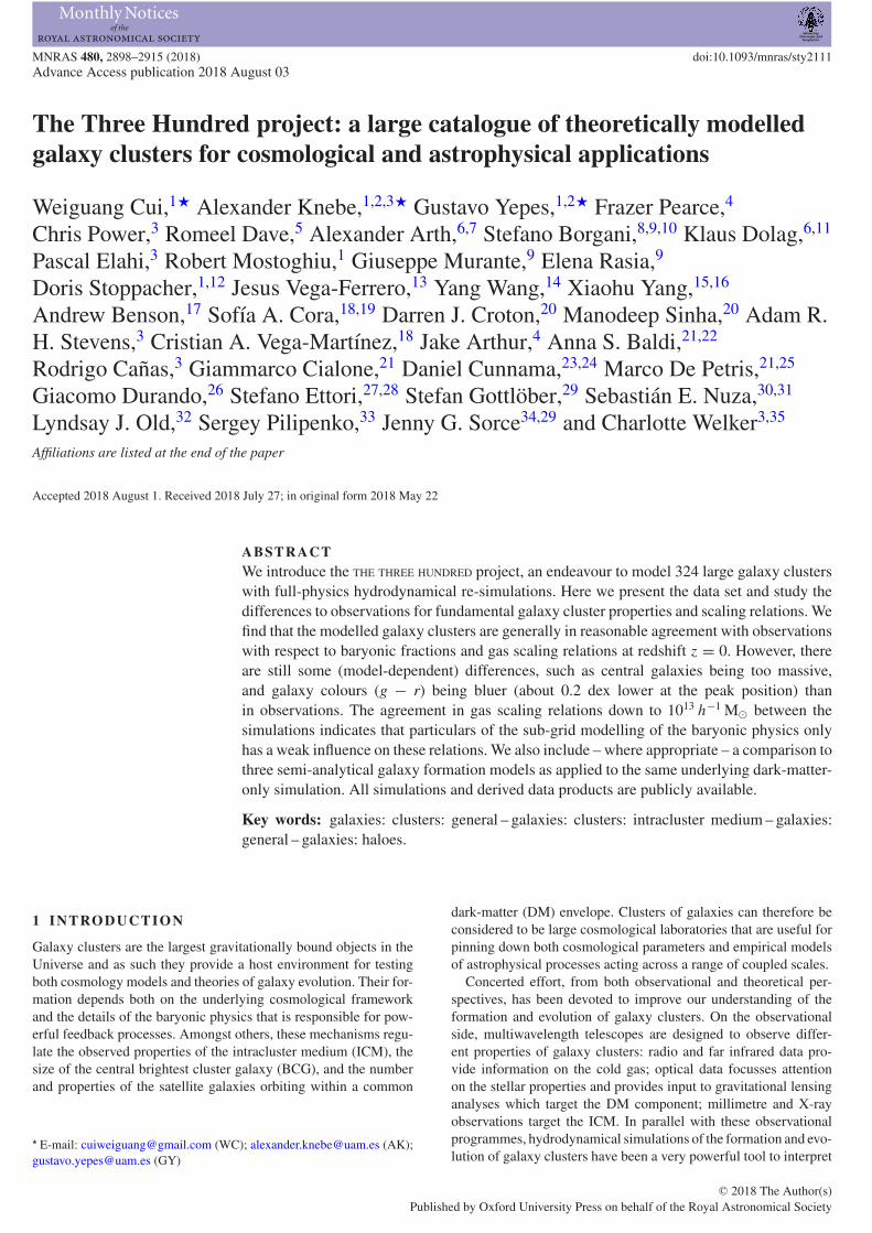
MNRAS 480, 2898–2915 (2018) doi:10.1093/mnras/sty2111Advance Access publication 2018 August 03

The Three Hundred project: a large catalogue of theoretically modelledgalaxy clusters for cosmological and astrophysical applications

Weiguang Cui,1‹ Alexander Knebe,1,2,3‹ Gustavo Yepes,1,2‹ Frazer Pearce,4

Chris Power,3 Romeel Dave,5 Alexander Arth,6,7 Stefano Borgani,8,9,10 Klaus Dolag,6,11

Pascal Elahi,3 Robert Mostoghiu,1 Giuseppe Murante,9 Elena Rasia,9

Doris Stoppacher,1,12 Jesus Vega-Ferrero,13 Yang Wang,14 Xiaohu Yang,15,16

Andrew Benson,17 Sofıa A. Cora,18,19 Darren J. Croton,20 Manodeep Sinha,20 Adam R.H. Stevens,3 Cristian A. Vega-Martınez,18 Jake Arthur,4 Anna S. Baldi,21,22

Rodrigo Canas,3 Giammarco Cialone,21 Daniel Cunnama,23,24 Marco De Petris,21,25

Giacomo Durando,26 Stefano Ettori,27,28 Stefan Gottlober,29 Sebastian E. Nuza,30,31

Lyndsay J. Old,32 Sergey Pilipenko,33 Jenny G. Sorce34,29 and Charlotte Welker3,35

Affiliations are listed at the end of the paper

Accepted 2018 August 1. Received 2018 July 27; in original form 2018 May 22

ABSTRACTWe introduce the THE THREE HUNDRED project, an endeavour to model 324 large galaxy clusterswith full-physics hydrodynamical re-simulations. Here we present the data set and study thedifferences to observations for fundamental galaxy cluster properties and scaling relations. Wefind that the modelled galaxy clusters are generally in reasonable agreement with observationswith respect to baryonic fractions and gas scaling relations at redshift z = 0. However, thereare still some (model-dependent) differences, such as central galaxies being too massive,and galaxy colours (g − r) being bluer (about 0.2 dex lower at the peak position) thanin observations. The agreement in gas scaling relations down to 1013 h−1 M⊙ between thesimulations indicates that particulars of the sub-grid modelling of the baryonic physics onlyhas a weak influence on these relations. We also include – where appropriate – a comparison tothree semi-analytical galaxy formation models as applied to the same underlying dark-matter-only simulation. All simulations and derived data products are publicly available.

Key words: galaxies: clusters: general – galaxies: clusters: intracluster medium – galaxies:general – galaxies: haloes.

1 IN T RO D U C T I O N

Galaxy clusters are the largest gravitationally bound objects in theUniverse and as such they provide a host environment for testingboth cosmology models and theories of galaxy evolution. Their for-mation depends both on the underlying cosmological frameworkand the details of the baryonic physics that is responsible for pow-erful feedback processes. Amongst others, these mechanisms regu-late the observed properties of the intracluster medium (ICM), thesize of the central brightest cluster galaxy (BCG), and the numberand properties of the satellite galaxies orbiting within a common

⋆ E-mail: cuiweiguang@gmail.com (WC); alexander.knebe@uam.es (AK);gustavo.yepes@uam.es (GY)

dark-matter (DM) envelope. Clusters of galaxies can therefore beconsidered to be large cosmological laboratories that are useful forpinning down both cosmological parameters and empirical modelsof astrophysical processes acting across a range of coupled scales.

Concerted effort, from both observational and theoretical per-spectives, has been devoted to improve our understanding of theformation and evolution of galaxy clusters. On the observationalside, multiwavelength telescopes are designed to observe differ-ent properties of galaxy clusters: radio and far infrared data pro-vide information on the cold gas; optical data focusses attentionon the stellar properties and provides input to gravitational lensinganalyses which target the DM component; millimetre and X-rayobservations target the ICM. In parallel with these observationalprogrammes, hydrodynamical simulations of the formation and evo-lution of galaxy clusters have been a very powerful tool to interpret

C⃝ 2018 The Author(s)Published by Oxford University Press on behalf of the Royal Astronomical Society

Dow

nloaded from https://academ

ic.oup.com/m

nras/article-abstract/480/3/2898/5066184 by Konkoly Observatory user on 23 Septem

ber 2019

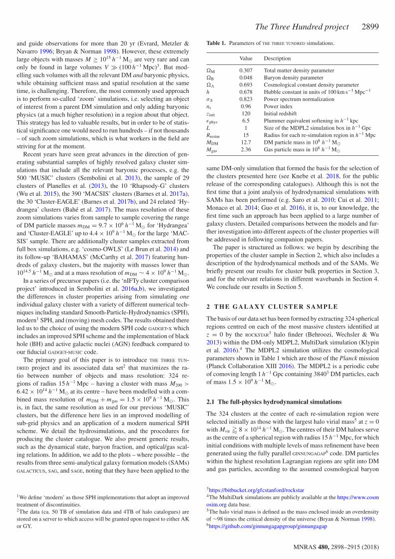
The Three Hundred project 2899

and guide observations for more than 20 yr (Evrard, Metzler &Navarro 1996; Bryan & Norman 1998). However, these extremelylarge objects with masses M ≥ 1015 h−1 M⊙ are very rare and canonly be found in large volumes V ≫ (100 h−1 Mpc)3. But mod-elling such volumes with all the relevant DM and baryonic physics,while obtaining sufficient mass and spatial resolution at the sametime, is challenging. Therefore, the most commonly used approachis to perform so-called ‘zoom’ simulations, i.e. selecting an objectof interest from a parent DM simulation and only adding baryonicphysics (at a much higher resolution) in a region about that object.This strategy has led to valuable results, but in order to be of statis-tical significance one would need to run hundreds – if not thousands– of such zoom simulations, which is what workers in the field arestriving for at the moment.

Recent years have seen great advances in the direction of gen-erating substantial samples of highly resolved galaxy cluster sim-ulations that include all the relevant baryonic processes, e.g. the500 ‘MUSIC’ clusters (Sembolini et al. 2013), the sample of 29clusters of Planelles et al. (2013), the 10 ‘Rhapsody-G’ clusters(Wu et al. 2015), the 390 ‘MACSIS’ clusters (Barnes et al. 2017a),the 30 ‘Cluster-EAGLE’ (Barnes et al. 2017b), and 24 related ‘Hy-drangea’ clusters (Bahe et al. 2017). The mass resolution of thesezoom simulations varies from sample to sample covering the rangeof DM particle masses mDM = 9.7 × 106 h−1 M⊙ for ‘Hydrangea’and ‘Cluster-EAGLE’ up to 4.4 × 109 h−1 M⊙ for the large ‘MAC-SIS’ sample. There are additionally cluster samples extracted fromfull box simulations, e.g. ‘cosmo-OWLS’ (Le Brun et al. 2014) andits follow-up ‘BAHAMAS’ (McCarthy et al. 2017) featuring hun-dreds of galaxy clusters, but the majority with masses lower than1014.5 h−1 M⊙ and at a mass resolution of mDM ∼ 4 × 109 h−1 M⊙.

In a series of precursor papers (i.e. the ‘nIFTy cluster comparisonproject’ introduced in Sembolini et al. 2016a,b), we investigatedthe differences in cluster properties arising from simulating oneindividual galaxy cluster with a variety of different numerical tech-niques including standard Smooth-Particle-Hydrodynamics (SPH),modern1 SPH, and (moving) mesh codes. The results obtained thereled us to the choice of using the modern SPH code GADGET-X whichincludes an improved SPH scheme and the implementation of blackhole (BH) and active galactic nuclei (AGN) feedback compared toour fiducial GADGET-MUSIC code.

The primary goal of this paper is to introduce THE THREE TUN-DRED project and its associated data set2 that maximizes the ra-tio between number of objects and mass resolution: 324 re-gions of radius 15 h−1 Mpc – having a cluster with mass M200 >

6.42 × 1014 h−1 M⊙ at its centre – have been modelled with a com-bined mass resolution of mDM + mgas = 1.5 × 109 h−1 M⊙. Thisis, in fact, the same resolution as used for our previous ‘MUSIC’clusters, but the difference here lies in an improved modelling ofsub-grid physics and an application of a modern numerical SPHscheme. We detail the hydrosimulations, and the procedures forproducing the cluster catalogue. We also present generic results,such as the dynamical state, baryon fraction, and optical/gas scal-ing relations. In addition, we add to the plots – where possible – theresults from three semi-analytical galaxy formation models (SAMs)GALACTICUS, SAG, and SAGE, noting that they have been applied to the

1We define ‘modern’ as those SPH implementations that adopt an improvedtreatment of discontinuities.2The data (ca. 50 TB of simulation data and 4TB of halo catalogues) arestored on a server to which access will be granted upon request to either AKor GY.

Table 1. Parameters of THE THREE TUNDRED simulations.

Value Description

"M 0.307 Total matter density parameter"B 0.048 Baryon density parameter"# 0.693 Cosmological constant density parameterh 0.678 Hubble constant in units of 100 km s−1 Mpc−1

σ 8 0.823 Power spectrum normalizationns 0.96 Power indexzinit 120 Initial redshiftϵphys 6.5 Plummer equivalent softening in h−1 kpcL 1 Size of the MDPL2 simulation box in h−1 GpcRresim 15 Radius for each re-simulation region in h−1 MpcMDM 12.7 DM particle mass in 108 h−1 M⊙Mgas 2.36 Gas particle mass in 108 h−1 M⊙

same DM-only simulation that formed the basis for the selection ofthe clusters presented here (see Knebe et al. 2018, for the publicrelease of the corresponding catalogues). Although this is not thefirst time that a joint analysis of hydrodynamical simulations withSAMs has been performed (e.g. Saro et al. 2010; Cui et al. 2011;Monaco et al. 2014; Guo et al. 2016), it is, to our knowledge, thefirst time such an approach has been applied to a large number ofgalaxy clusters. Detailed comparisons between the models and fur-ther investigation into different aspects of the cluster properties willbe addressed in following companion papers.

The paper is structured as follows: we begin by describing theproperties of the cluster sample in Section 2, which also includes adescription of the hydrodynamical methods and of the SAMs. Webriefly present our results for cluster bulk properties in Section 3,and for the relevant relations in different wavebands in Section 4.We conclude our results in Section 5.

2 TH E G A L A X Y C L U S T E R SA M P L E

The basis of our data set has been formed by extracting 324 sphericalregions centred on each of the most massive clusters identified atz = 0 by the ROCKSTAR3 halo finder (Behroozi, Wechsler & Wu2013) within the DM-only MDPL2, MultiDark simulation (Klypinet al. 2016).4 The MDPL2 simulation utilizes the cosmologicalparameters shown in Table 1 which are those of the Planck mission(Planck Collaboration XIII 2016). The MDPL2 is a periodic cubeof comoving length 1 h−1 Gpc containing 38403 DM particles, eachof mass 1.5 × 109 h−1 M⊙.

2.1 The full-physics hydrodynamical simulations

The 324 clusters at the centre of each re-simulation region wereselected initially as those with the largest halo virial mass5 at z = 0with Mvir ! 8 × 1014 h−1 M⊙. The centres of their DM haloes serveas the centre of a spherical region with radius 15 h−1 Mpc, for whichinitial conditions with multiple levels of mass refinement have beengenerated using the fully parallel GINNUNGAGAP6 code. DM particleswithin the highest resolution Lagrangian regions are split into DMand gas particles, according to the assumed cosmological baryon

3https://bitbucket.org/gfcstanford/rockstar4The MultiDark simulations are publicly available at the https://www.cosmosim.org data base.5The halo virial mass is defined as the mass enclosed inside an overdensityof ∼98 times the critical density of the universe (Bryan & Norman 1998).6https://github.com/ginnungagapgroup/ginnungagap

MNRAS 480, 2898–2915 (2018)

Dow

nloaded from https://academ

ic.oup.com/m

nras/article-abstract/480/3/2898/5066184 by Konkoly Observatory user on 23 Septem

ber 2019

2900 W. Cui et al.

Table 2. Baryonic models for the two simulation codes.

Baryon physics GADGET-MUSIC GADGET-X

Gas treatmentHomogeneous UV background Haardt & Madau (2001) Haardt & Madau (1996)Cooling Metal independent Metal dependent (Wiersma, Schaye & Smith 2009)Star formation and stellar feedbackStellar model Springel & Hernquist (2003) Tornatore et al. (2007)Threshold for star forming 0.1 cm−3 0.1 cm−3

IMF Salpeter (1955) Chabrier (2003)Kinetic feedback Springel & Hernquist (2003) Springel & Hernquist (2003)Wind velocity 400 km s−1 350 km s−1

Thermal feedback 2-phase model (Yepes et al. 1997) Only set the hot phase temperatureGas mass-loss via galactic winds NoBH and AGN feedbackBH seeding No Mbh = 5 × 106 h−1 M⊙ for

MFoF ≥ 2.5 × 1011 h−1 M⊙BH growth No Individual accretion of hot and cold gasAGN feedback No Steinborn et al. (2015)

fraction listed in Table 1. Our mass resolution is a factor of threebetter than that used for the 390 ‘MACSIS’ clusters (Barnes et al.2017a). We further highlight that our re-simulation regions havethe same mass resolution as the original DM-only simulation uponwhich the SAMs are based. The DM particles outside this regionare successively degraded in multiple layers (with a shell thicknessof ∼4 h−1 Mpc) with lower mass resolution particles (increased byeight times for each layer) that eventually provide the same tidalfields yet at a much lower computational costs than in the originalsimulation.7 The size of the re-simulated region is much larger thanthe virial radius of the cluster it surrounds. As such, each region alsocontains many additional groups and filamentary structure that mayor may not be physically associated with the cluster they surround.

The initial conditions – also publicly available – were run withthe ‘modern’ SPH code GADGET-X and snapshots of the simulationsstored for a set of pre-selected redshifts. A total of 128 differentsnapshots have been stored for each simulation from redshift z =17 to 0. We also ran the same simulations with our fiducial GADGET-MUSIC code (Sembolini et al. 2013). Both codes are based on thegravity solver of the GADGET3 Tree-PM code (an updated version ofthe GADGET2 code; Springel 2005). While both use smooth-particlehydrodynamics (SPH) to follow the evolution of the gas compo-nent, they apply different SPH techniques as well as rather dis-tinct models for the sub-resolution physics. GADGET-X includes animproved SPH scheme (Beck et al. 2016) with artificial thermaldiffusion, time-dependent artificial viscosity, high-order WendlandC4 interpolating kernel, and wake-up scheme. These improvementsadvance the SPH capability of following gas-dynamical instabilitiesand mixing processes by better describing the discontinuities andreducing the clumpiness instability of gas. They also minimize theviscosity away from shock regions and especially in rotating shears.GADGET-MUSIC uses the classic entropy-conserving SPH formulationwith a 40 neighbour M3 interpolation kernel. The differences inbaryon treatment have been summarized in Table 2. For more de-tails and the implications of the code differences we refer the readerto our comparison papers (Sembolini et al. 2016a,b).

7The initial conditions for these clusters are publicly available in GADGET

format and can be downloaded from http://music.ft.uam.es upon request.We have also produced higher resolution initial conditions corresponding toan equivalent resolution of 76803 particles, for a subsample of the clustercatalogue.

All data were then analysed with a standardized pipeline thatincludes the AHF8 (Knollmann & Knebe 2009) halo finder whichself-consistently includes both gas and stars in the halo finding pro-cess. For each halo, we compute the radius R200, that is the radiusr at which the density M(< r)/(4πr3/3) drops below 200ρcrit.9 Hereρcrit is the critical density of the Universe at the respective redshift.Subhaloes are defined as haloes which lie within the R200 regionof a more massive halo, the so-called host halo. As subhaloes areembedded within the density of their respective host halo, theirown density profile usually shows a characteristic upturn at a radiusRt " R200, where R200 would be their actual radius if they werefound in isolation. We use this ‘truncation radius’ Rt as the outeredge of the subhalo and hence subhalo properties (i.e. mass, densityprofile, velocity dispersion, rotation curve) are calculated using thegravitationally bound particles inside the truncation radius Rt. Fora host halo that contains the mass of their subhaloes, we calculateproperties using the radius R200. Halo merger trees, that link objectsbetween different redshifts, were constructed using MERGERTREE thatforms part of the AHF package. We have calculated luminosities indifferent spectral bands from the stars within the haloes by apply-ing the stellar population synthesis code STARDUST (see Devriendt,Guiderdoni & Sadat 1999, and references therein for more details).This code computes the spectral energy distribution from far-UVto radio, for an instantaneous starburst of a given mass, age, andmetallicity. The stellar contribution to the total flux is calculatedassuming a Kennicutt initial mass function (Kennicutt 1998).

The full data set consists of 324 re-simulated regions, which covera much larger volume (out to 15 h−1 Mpc in radius) than the cen-tral halo’s virial radius and hence our sample includes many otherobjects outside that sphere. These objects are composed of haloes,groups, and filaments, which allow us to investigate the preprocess-ing of the galaxy cluster as well as its large-scale environment. Assome of the objects close to the boundary could be contaminatedby low-resolution particles in the hydrodynamic simulations, weexplicitly checked that all the objects included in the comprehen-sive catalogue do not contain any low-resolution particles. In whatfollows we refer to this data set, which consists of all the uncon-

8http://popia.ft.uam.es/AHF9Similarly, the subscript 500 used in this paper later are for haloes definedwith enclosed overdensities of 500 times the critical density of the universe.

MNRAS 480, 2898–2915 (2018)

Dow

nloaded from https://academ

ic.oup.com/m

nras/article-abstract/480/3/2898/5066184 by Konkoly Observatory user on 23 Septem

ber 2019

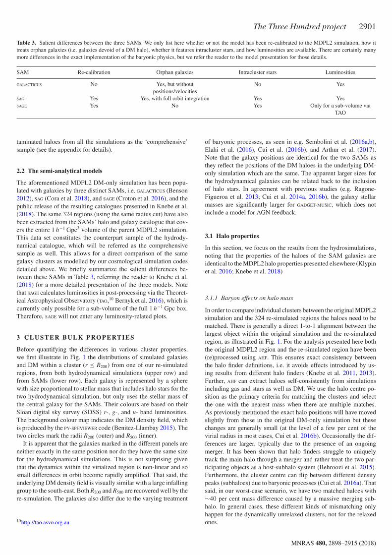
The Three Hundred project 2901

Table 3. Salient differences between the three SAMs. We only list here whether or not the model has been re-calibrated to the MDPL2 simulation, how ittreats orphan galaxies (i.e. galaxies devoid of a DM halo), whether it features intracluster stars, and how luminosities are available. There are certainly manymore differences in the exact implementation of the baryonic physics, but we refer the reader to the model presentation for those details.

SAM Re-calibration Orphan galaxies Intracluster stars Luminosities

GALACTICUS No Yes, but withoutpositions/velocities

No Yes

SAG Yes Yes, with full orbit integration Yes YesSAGE Yes No Yes Only for a sub-volume via

TAO

taminated haloes from all the simulations as the ‘comprehensive’sample (see the appendix for details).

2.2 The semi-analytical models

The aforementioned MDPL2 DM-only simulation has been popu-lated with galaxies by three distinct SAMs, i.e. GALACTICUS (Benson2012), SAG (Cora et al. 2018), and SAGE (Croton et al. 2016), and thepublic release of the resulting catalogues presented in Knebe et al.(2018). The same 324 regions (using the same radius cut) have alsobeen extracted from the SAMs’ halo and galaxy catalogue that cov-ers the entire 1 h−1 Gpc3 volume of the parent MDPL2 simulation.This data set constitutes the counterpart sample of the hydrody-namical catalogue, which will be referred as the comprehensivesample as well. This allows for a direct comparison of the samegalaxy clusters as modelled by our cosmological simulation codesdetailed above. We briefly summarize the salient differences be-tween these SAMs in Table 3, referring the reader to Knebe et al.(2018) for a more detailed presentation of the three models. Notethat SAGE calculates luminosities in post-processing via the Theoret-ical Astrophysical Observatory (TAO,10 Bernyk et al. 2016), which iscurrently only possible for a sub-volume of the full 1 h−1 Gpc box.Therefore, SAGE will not enter any luminosity-related plots.

3 C LUSTER BU LK PROPERTIES

Before quantifying the differences in various cluster properties,we first illustrate in Fig. 1 the distributions of simulated galaxiesand DM within a cluster (r ≤ R200) from one of our re-simulatedregions, from both hydrodynamical simulations (upper row) andfrom SAMs (lower row). Each galaxy is represented by a spherewith size proportional to stellar mass that includes halo stars for thetwo hydrodynamical simulation, but only uses the stellar mass ofthe central galaxy for the SAMs. Their colours are based on theirSloan digital sky survey (SDSS) r-, g-, and u- band luminosities.The background colour map indicates the DM density field, whichis produced by the PY-SPHVIEWER code (Benitez-Llambay 2015). Thetwo circles mark the radii R200 (outer) and R500 (inner).

It is apparent that the galaxies marked in the different panels areneither exactly in the same position nor do they have the same sizefor the hydrodynamical simulations. This is not surprising giventhat the dynamics within the virialized region is non-linear and sosmall differences in orbit become rapidly amplified. That said, theunderlying DM density field is visually similar with a large infallinggroup to the south-east. Both R200 and R500 are recovered well by there-simulation. The galaxies also differ due to the varying treatment

10http://tao.asvo.org.au

of baryonic processes, as seen in e.g. Sembolini et al. (2016a,b),Elahi et al. (2016), Cui et al. (2016b), and Arthur et al. (2017).Note that the galaxy positions are identical for the two SAMs asthey reflect the positions of the DM haloes in the underlying DM-only simulation which are the same. The apparent larger sizes forthe hydrodynamical galaxies can be related back to the inclusionof halo stars. In agreement with previous studies (e.g. Ragone-Figueroa et al. 2013; Cui et al. 2014a, 2016b), the galaxy stellarmasses are significantly larger for GADGET-MUSIC, which does notinclude a model for AGN feedback.

3.1 Halo properties

In this section, we focus on the results from the hydrosimulations,noting that the properties of the haloes of the SAM galaxies areidentical to the MDPL2 halo properties presented elsewhere (Klypinet al. 2016; Knebe et al. 2018)

3.1.1 Baryon effects on halo mass

In order to compare individual clusters between the original MDPL2simulation and the 324 re-simulated regions the haloes need to bematched. There is generally a direct 1-to-1 alignment between thelargest object within the original simulation and the re-simulatedregion, as illustrated in Fig. 1. For the analysis presented here boththe original MDPL2 region and the re-simulated region have been(re)processed using AHF. This ensures exact consistency betweenthe halo finder definitions, i.e. it avoids effects introduced by us-ing results from different halo finders (Knebe et al. 2011, 2013).Further, AHF can extract haloes self-consistently from simulationsincluding gas and stars as well as DM. We use the halo centre po-sition as the primary criteria for matching the clusters and selectthe one with the nearest mass when there are multiple matches.As previously mentioned the exact halo positions will have movedslightly from those in the original DM-only simulation but thesechanges are generally small (at the level of a few per cent of thevirial radius in most cases, Cui et al. 2016b). Occasionally the dif-ferences are larger, typically due to the presence of an ongoingmerger. It has been shown that halo finders struggle to uniquelytrack the main halo through a merger and rather treat the two par-ticipating objects as a host-subhalo system (Behroozi et al. 2015).Furthermore, the cluster centre can flip between different densitypeaks (subhaloes) due to baryonic processes (Cui et al. 2016a). Thatsaid, in our worst-case scenario, we have two matched haloes with∼40 per cent mass difference caused by a massive merging sub-halo. In general cases, these different kinds of mismatching onlyhappen for the dynamically unrelaxed clusters, not for the relaxedones.

MNRAS 480, 2898–2915 (2018)

Dow

nloaded from https://academ

ic.oup.com/m

nras/article-abstract/480/3/2898/5066184 by Konkoly Observatory user on 23 Septem

ber 2019

2902 W. Cui et al.

Figure 1. The distribution of galaxies within R200 of the most massive cluster within re-simulation region 1. The upper row shows the results from GADGET-MUSIC

(left-hand side) and GADGET-X (right-hand side). The lower row shows the results from the SAMs GALACTICUS (left-hand side) and SAG (right-hand side). Theprojected DM density is shown in the background with a blue-red colour map. Galaxy colour is taken from their SDSS r, g, and u band magnitude and thesymbol size is proportional to stellar mass. The two circles mark the radii R200 (outer circle) and R500 (inner circle).

Accurate estimates of cluster masses are very important for con-straining cosmological parameters and cosmological models (e.g.Bocquet et al. 2016; Sartoris et al. 2016). Therefore, we presenthere a quantitative comparison of the halo masses as found in thehydrodynamical simulations with their respective counterparts fromthe DM-only MDPL2 simulation (see Cui & Zhang 2017, for a re-view of the baryon effect). Fig. 2 shows the mass ratio of clustersin GADGET-MUSIC (red circle and lines) and GADGET-X (blue star and

lines) to their MDPL2 counterparts; M200 is shown in the left-handside panel and M500 in the right-hand side panel.11 In order to reduceany issues due to mismatching, we select a sample of dynamically

11The M500 sample was constructed by using AHF to find the largest halocontained within each of the 324 clusters of the mass-complete sample (andmatching these as before).

MNRAS 480, 2898–2915 (2018)

Dow

nloaded from https://academ

ic.oup.com/m

nras/article-abstract/480/3/2898/5066184 by Konkoly Observatory user on 23 Septem

ber 2019

The Three Hundred project 2903

Figure 2. The mass ratio between matched clusters at z = 0 identified in the hydrodynamical simulations (Mhydro) and in the corresponding cosmologicalDM-only run MDPL2 (MDM) for M200 (left-hand side panel) and M500 (right-hand side panel) as a function of MDM. The complete sample used here is inthin lines, while the dynamically relaxed subsample is in thick lines. The median value for each mass bin is shown via the symbols (red dots for GADGET-MUSIC

and blue stellar symbols for GADGET-X) with error bars indicating the 16th and 84th percentiles. The black horizontal long-dashed and dotted lines indicateequivalent mass and 1 per cent variation, respectively.

relaxed clusters (see below for details) from the complete sampleand repeat the comparison. The mass ratio for M200 from both hy-drodynamical simulations is very close to unity (with the mediandifference lying basically within 1 per cent), with a scatter less than∼5 per cent (∼2.5 per cent for the relaxed subsample). At the low-mass end, GADGET-X (for both samples) tends to have about 1 percent higher mass than its MDPL2 counterpart. However, the M500

mass in both sets of hydrodynamical simulations tends to be sev-eral (up to 6) per cent higher than its DM-only counterpart below∼9 × 1014 h−1 M⊙. Above this halo mass the ratio drops to around1 again. It is worth noting that for M500 there is a larger scatter of∼8 per cent for the complete sample and ∼4 per cent for the relaxedsubsample. We ascribe this larger mass change for M500 to baryonicprocesses that have a larger effect closer to the cluster’s centre andfor the less massive haloes. The two simulation codes show similarresults for M # 1015 h−1 M⊙ at both overdensities, which meansthat the baryon physics has little influence on both M500 and M200 atthis cluster mass range. For the M200 mass changes, this is in agree-ment with previous similar comparisons (e.g. Cui et al. 2012; Cui,Borgani & Murante 2014b; Cui et al. 2016b). For M500, Cui et al.(2014b) reported a slight mass decrease when an AGN feedbackis included and a slight mass increase without the AGN feedback.At this halo mass range, M500 > 1014.5 h−1 M⊙, the difference be-tween GADGET-X and Cui et al. (2014b) could be caused by eithera sample effect (Cui et al. 2014b studied very few clusters) or dueto the details of the baryonic model implemented in the simulation.We will explore this in detail in a follow-up paper (Cui et al. inpreparation) which will also focus on cluster mass estimates basedupon different observational methods applied to our simulationdata.

3.1.2 Dynamical relaxation

To determine the dynamical state of the cluster sample we studythree indicators, following Cui et al. (2017), specifically:

(i) the virial ratio η = (2T − Es)/|W|, where T is the total kineticenergy, Es is the energy from surface pressure, and W is the totalpotential energy,

(ii) the centre-of-mass offset )r = |Rcm − Rc|/R200, where Rcm isthe centre-of-mass within a cluster radius of R200, Rc is the centre ofthe cluster corresponding to the maximum density peak of the halo.Using the position of the minimum of the gravitational potentialwould give a similar result as investigated by Cui et al. (2016a).

(iii) the fraction of mass in subhaloes fs =!

Msub/M200 whereMsub is the mass of each subhalo.

We adopt the following criteria to select dynamically relaxedclusters: 0.85 < η < 1.15, )r < 0.04 and fs < 0.1, which need tobe satisfied at the same time (see, for instance, Neto et al. 2007;Knebe et al. 2008; Power, Knebe & Knollmann 2012). Note thatwe use here a slightly larger limit for fs than in Cui et al. (2017).This is because (1) R200 is used instead of the virial radius,12 and(2) this threshold for fs gives a relaxation fraction (∼20 per cent forboth hydrodynamical simulations) comparable to observations (e.g.Mantz et al. 2015; Biffi et al. 2016).

In Fig. 3, we show the relations between these three parame-ters for the mass-complete sample: )r versus η in the left-hand

12Note that for the given cosmology R200 < Rvir and hence the M200 massesof the host haloes considered here will be about 25 per cent smaller thanMvir.

MNRAS 480, 2898–2915 (2018)

Dow

nloaded from https://academ

ic.oup.com/m

nras/article-abstract/480/3/2898/5066184 by Konkoly Observatory user on 23 Septem

ber 2019

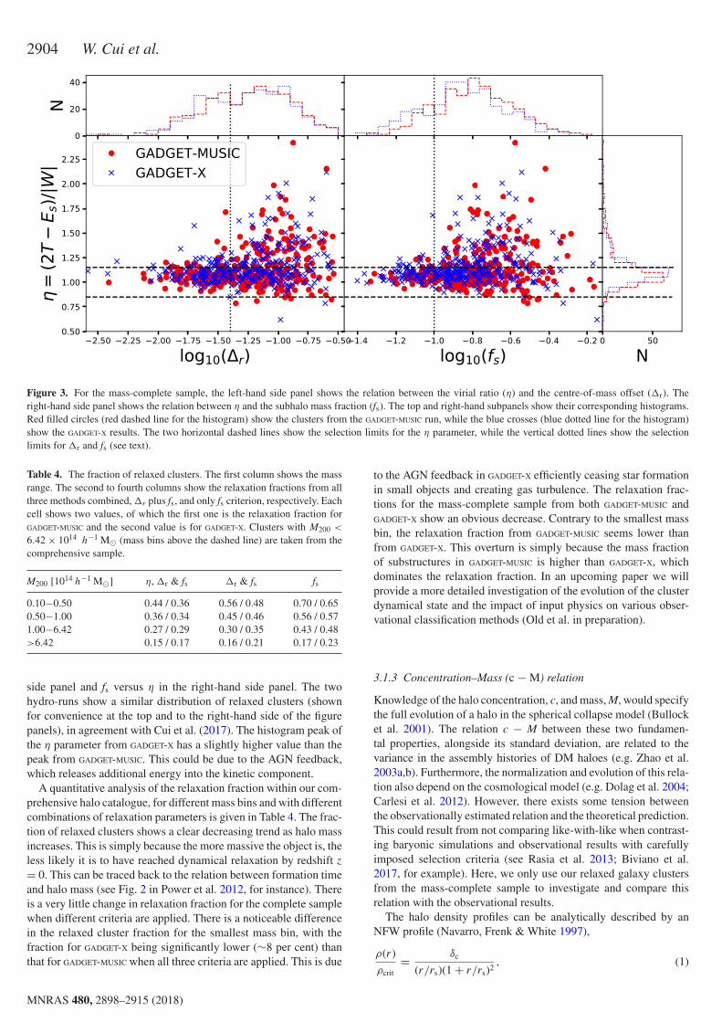
2904 W. Cui et al.

Figure 3. For the mass-complete sample, the left-hand side panel shows the relation between the virial ratio (η) and the centre-of-mass offset ()r). Theright-hand side panel shows the relation between η and the subhalo mass fraction (fs). The top and right-hand subpanels show their corresponding histograms.Red filled circles (red dashed line for the histogram) show the clusters from the GADGET-MUSIC run, while the blue crosses (blue dotted line for the histogram)show the GADGET-X results. The two horizontal dashed lines show the selection limits for the η parameter, while the vertical dotted lines show the selectionlimits for )r and fs (see text).

Table 4. The fraction of relaxed clusters. The first column shows the massrange. The second to fourth columns show the relaxation fractions from allthree methods combined, )r plus fs, and only fs criterion, respectively. Eachcell shows two values, of which the first one is the relaxation fraction forGADGET-MUSIC and the second value is for GADGET-X. Clusters with M200 <

6.42 × 1014 h−1 M⊙ (mass bins above the dashed line) are taken from thecomprehensive sample.

M200 [1014 h−1 M⊙] η, )r & fs )r & fs fs

0.10−0.50 0.44 / 0.36 0.56 / 0.48 0.70 / 0.650.50−1.00 0.36 / 0.34 0.45 / 0.46 0.56 / 0.571.00−6.42 0.27 / 0.29 0.30 / 0.35 0.43 / 0.48>6.42 0.15 / 0.17 0.16 / 0.21 0.17 / 0.23

side panel and fs versus η in the right-hand side panel. The twohydro-runs show a similar distribution of relaxed clusters (shownfor convenience at the top and to the right-hand side of the figurepanels), in agreement with Cui et al. (2017). The histogram peak ofthe η parameter from GADGET-X has a slightly higher value than thepeak from GADGET-MUSIC. This could be due to the AGN feedback,which releases additional energy into the kinetic component.

A quantitative analysis of the relaxation fraction within our com-prehensive halo catalogue, for different mass bins and with differentcombinations of relaxation parameters is given in Table 4. The frac-tion of relaxed clusters shows a clear decreasing trend as halo massincreases. This is simply because the more massive the object is, theless likely it is to have reached dynamical relaxation by redshift z

= 0. This can be traced back to the relation between formation timeand halo mass (see Fig. 2 in Power et al. 2012, for instance). Thereis a very little change in relaxation fraction for the complete samplewhen different criteria are applied. There is a noticeable differencein the relaxed cluster fraction for the smallest mass bin, with thefraction for GADGET-X being significantly lower (∼8 per cent) thanthat for GADGET-MUSIC when all three criteria are applied. This is due

to the AGN feedback in GADGET-X efficiently ceasing star formationin small objects and creating gas turbulence. The relaxation frac-tions for the mass-complete sample from both GADGET-MUSIC andGADGET-X show an obvious decrease. Contrary to the smallest massbin, the relaxation fraction from GADGET-MUSIC seems lower thanfrom GADGET-X. This overturn is simply because the mass fractionof substructures in GADGET-MUSIC is higher than GADGET-X, whichdominates the relaxation fraction. In an upcoming paper we willprovide a more detailed investigation of the evolution of the clusterdynamical state and the impact of input physics on various obser-vational classification methods (Old et al. in preparation).

3.1.3 Concentration–Mass (c − M) relation

Knowledge of the halo concentration, c, and mass, M, would specifythe full evolution of a halo in the spherical collapse model (Bullocket al. 2001). The relation c − M between these two fundamen-tal properties, alongside its standard deviation, are related to thevariance in the assembly histories of DM haloes (e.g. Zhao et al.2003a,b). Furthermore, the normalization and evolution of this rela-tion also depend on the cosmological model (e.g. Dolag et al. 2004;Carlesi et al. 2012). However, there exists some tension betweenthe observationally estimated relation and the theoretical prediction.This could result from not comparing like-with-like when contrast-ing baryonic simulations and observational results with carefullyimposed selection criteria (see Rasia et al. 2013; Biviano et al.2017, for example). Here, we only use our relaxed galaxy clustersfrom the mass-complete sample to investigate and compare thisrelation with the observational results.

The halo density profiles can be analytically described by anNFW profile (Navarro, Frenk & White 1997),

ρ(r)ρcrit

= δc

(r/rs)(1 + r/rs)2, (1)

MNRAS 480, 2898–2915 (2018)

Dow

nloaded from https://academ

ic.oup.com/m

nras/article-abstract/480/3/2898/5066184 by Konkoly Observatory user on 23 Septem

ber 2019

The Three Hundred project 2905

which is characterized by the two parameters, rs and δc. The con-centration c200 is then given by R200/rs. We fit our simulated clusterdensity profiles, defined by equally spaced log-bins, to this func-tional form with both parameters free, but exclude the very centralregion in this process. Due to the presence of the BCG, the mass pro-file in the centre is much steeper than the total mass profile (Schalleret al. 2015b). As the edge of the BCG is not clearly defined, we adopttwo different inner ‘exclusion’ radii during the fitting: 0.05 R200, assuggested by, for example, Schaller et al. (2015b), Cui et al. (2016b),and ∼34 h−1 kpc following Biviano et al. (2017). We have verifiedthat the NFW profile provides a good fit regardless of the adoptedinner radii (34 h−1 kpc or 0.05 R200). In both cases the differencebetween the fit and the original density profile is within 20 per centat all radii.

In the left-hand side panel of Fig. 4 we show the c − M relationfor our relaxed galaxy clusters and compare the relation with obser-vational results coming from both X-ray and optical data obtainedwith different techniques (please refer to the figure caption and leg-end, respectively). For each of the two hydrodynamical simulationcodes, we show results stemming from either truncation approach:circles for using the range [0.05 R200 − R200] and stars for a fixedinner radius of 34 h−1 kpc. We fit our c − M relation using thefollowing analytical function:

log10 c200 = α − β log10(M200/M⊙). (2)

The fitting parameters α and β are listed in Table 5.It is evident that the c − M relation from our hydrosimulated clus-

ters is closer to the observational results from Merten et al. (2015),Okabe & Smith (2016), and Biviano et al. (2017) than those fromMantz et al. (2016) and Groener et al. (2016). The c − M relationfrom the GADGET-MUSIC run is slightly higher than from the GADGET-X

run and it is in better agreement with observational results whichhave lower concentrations. It is obvious that the concentrations witha 34 h−1 kpc inner cut-off are systematically higher than the oneswith a 0.05 R200 cut-off (see also Rasia et al. 2013, for similar re-sults with different inner radii). Our fitted c − M relation fromthe GADGET-X clusters is much flatter than Schaller et al. (2015a),simply because their fit covers a much larger mass range, which isdominated by the lower mass objects. Furthermore, GADGET-X showsan increasing slope with β = −0.01 when a fixed inner radius of34 h−1 kpc is taken. This can be understood because 34 h−1 kpccorresponds to a smaller fraction of R200 for a massive cluster thanfor a less massive halo. Therefore it is not surprising to see a rela-tively high concentration for the most massive haloes when a fixedphysical cut-off radius is applied.

In the right-hand side panel of Fig. 4, we investigate the baryoneffects on the c − M relation by showing the relative change inconcentration from DM-only simulated clusters to their equivalentin the two hydro-runs. The change on c − M relation due to baryonsvaries from ∼25 per cent (for both radii) for GADGET-X to about 1.5–2times (0.05R200 - 34 h−1 kpc) for GADGET-MUSIC. However, this ratiois much lower for the highest mass bin for GADGET-X with both innerradii (also for GADGET-MUSIC with the inner radius of 34 h−1 kpc).The influence of baryons on the concentration is a little higher thanin Rasia et al. (2013), which may be the result of both the differentradius range used for profile fitting and differences in the baryonicmodel employed.

3.2 Baryon fractions

The formation of a galaxy cluster depends not only on gravity actingon cosmic scales but also on subresolution phenomena such as star

formation and various feedback mechanisms returning energy backto the intracluster gas. It is a process that involves interplay betweendark and baryonic matter. One of the most important quantities toquantify the relation between DM and baryons is the baryonic massfraction. It has therefore been intensively studied: on the theoret-ical side, mostly by means of hydrodynamical simulations (e.g.Planelles et al. 2013; Sembolini et al. 2013; Wu et al. 2015; Barneset al. 2017b); on the observational side via multiwavelength ob-servations (e.g. Lagana et al. 2013; Eckert et al. 2016; Chiu et al.2017).

In Fig. 5, we show the gas and stellar mass fractions for thecomprehensive sample from hydrodynamical simulations withinR500. The gas fraction for GADGET-X is larger than for GADGET-MUSIC atthe massive end, and drops more quickly towards lower mass haloes.The gas fraction from GADGET-X shows a better agreement with thedata of Gonzalez et al. (2013) at the massive end; both simulationsare in line with the results from Zhang et al. (2011) due to itslarge scatter. The offset between the two hydro-runs is much larger(a factor of 2–3) for the stellar fraction. Again, GADGET-X shows abetter agreement with the observational data points at the massiveend. However, it has a flatter slope than the observational results,which is close to the GADGET-MUSIC result at M500 " 1013.5 h−1 M⊙.This is possibly caused by the strong AGN feedback in GADGET-X.Essentially both hydrodynamic models have a stellar fraction versusmass slope that is inconsistent with the observational data.

Previous comparisons of the stellar and gas mass fractions fromfull-physics hydrodynamical simulations with observations haveshown that models without AGN feedback consistently have toolow a gas fraction and too high a stellar fraction due to the over-cooling problem (e.g. Planelles et al. 2013). This is also seen inFig. 5 comparing the GADGET-MUSIC and the GADGET-X runs. AlthoughGADGET-X tends to have a better agreement with the observationalresults, the AGN feedback implementation featured by this code isstill not perfect: the most massive clusters at M500 # 1015 h−1 M⊙still have a stellar fraction that is a little too high; while intermediateand low-mass haloes (M500 " 1014 h−1 M⊙) have stellar fractionsthat are too low. Nevertheless, we note that the stellar mass fractionestimated from observations is not without issues: there is relativeuncertainty about the contribution of the intracluster light (e.g. Zi-betti et al. 2005; Gonzalez, Zaritsky & Zabludoff 2007; Puchweinet al. 2010; Cui et al. 2014a), which is included in Gonzalez et al.(2013) and Kravtsov et al. (2018), but not in Zhang et al. (2011). An-other problem is the influence of the different initial mass functionsadopted in observations to derive stellar mass from luminosities(see e.g. Chiu et al. 2017, for detailed discussions).

The difference in the stellar mass fractions shows the importanceof the detailed prescription for baryon processes. Therefore, we areworking on a follow-up paper (Rasia et al., in preparation) to inves-tigate in detail the connection between the encapsulated physics andthe resultant baryonic fractions, examining the difference betweenrelaxed and unrelaxed clusters, between cool core and non-cool coreclusters, as well as the redshift evolution of these fractions.

4 ST E L L A R A N D G A S R E L AT I O N S O FC L US T E R S

Scaling relations between the total cluster mass and observationalquantities are derived in several multiwavelength studies. Com-monly used observational probes include stellar luminosity, X-raytemperature, or the Comptonization parameter (e.g. Reiprich &Bohringer 2002; Lin, Mohr & Stanford 2004; Andersson et al.2011), which normally show a self-similar relation to cluster mass.

MNRAS 480, 2898–2915 (2018)

Dow

nloaded from https://academ

ic.oup.com/m

nras/article-abstract/480/3/2898/5066184 by Konkoly Observatory user on 23 Septem

ber 2019

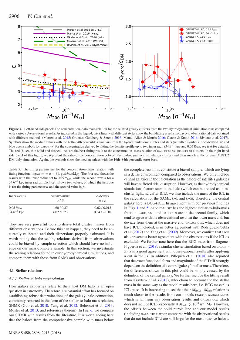
2906 W. Cui et al.

Figure 4. Left-hand side panel: The concentration–halo mass relation for the relaxed galaxy clusters from the two hydrodynamical simulation runs comparedwith various observational results. As indicated in the legend, thick lines with different styles show the best-fitting results from recent observational data obtainedwith different methods (Merten et al. 2015; Groener, Goldberg & Sereno 2016; Mantz, Allen & Morris 2016; Okabe & Smith 2016; Biviano et al. 2017).Symbols show the median values with the 16th–84th percentile error bars from the hydrosimulations: circles and stars (red filled symbols for GADGET-MUSIC andblue open symbols for GADGET-X) for the concentration derived by fitting the density profile up to two inner radii (34 h−1 kpc and 0.05 R200, see text for details).The red (blue), thin solid and dashed lines are the best-fitting result to the concentration–mass relation of GADGET-MUSIC (GADGET-X) clusters. In the right-handside panel of this figure, we represent the ratio of the concentration between the hydrodynamical simulation clusters and their match in the original MDPL2DM-only simulation. Again, the symbols show the median values with the 16th–84th percentile error bars.

Table 5. The fitting parameters for the concentration–mass relation withfitting function: log10c200 = α − βlog10M200/M⊙. The first row shows theresults with the inner radius set to 0.05 R200, while the second row is for a34 h−1 kpc inner radius. Each cell shows two values, of which the first oneis for the fitting parameter α and the second value is β.

Inner radius GADGET-MUSIC GADGET-X

α / β α / β

0.05 R200 4.60 / 0.27 0.62 / 0.01334 h−1 kpc 4.02 / 0.23 0.34 / −0.01

They are very powerful tools to derive total cluster masses fromdifferent observations. Before this can happen, they need to be ac-curately calibrated and their dispersions properly estimated. It isworth noting that the scaling relations derived from observationscould be biased by sample selection which should have no influ-ence on our mass-complete sample. In this section, we investigatethe scaling relations found in our hydrodynamical simulations, andcompare them with those from SAMs and observations.

4.1 Stellar relations

4.1.1 Stellar-to-halo mass relation

How galaxy properties relate to their host DM halo is an openquestion in astronomy. Therefore, a substantial effort has focused onestablishing robust determinations of the galaxy–halo connection,commonly reported in the form of the stellar-to-halo mass relation,SHMR (Guo et al. 2010; Yang et al. 2012; Behroozi et al. 2013;Moster et al. 2013, and references therein). In Fig. 6, we compareour SHMR with results from the literature. It is worth noting herethat the haloes from the comprehensive sample with mass below

the completeness limit constitute a biased sample, which are lyingin a dense environment compared to observations. We only includecentral galaxies in the calculation as the haloes of satellites galaxieswill have suffered tidal disruption. However, as the hydrodynamicalsimulations feature stars in the halo (which can be treated as intra-cluster light, hereafter ICL), we also include the mass of the ICL inthe calculation for the SAMs, SAG, and SAGE. Therefore, the centralgalaxy here is BCG+ICL. In agreement with our previous findingsin Figs 1 and 5, GADGET-MUSIC has the highest stellar-to-halo-massfraction. SAGE, SAG, and GADGET-X are in the second family, whichtend to agree with the observational result at the lower mass end, butdeviate from them at the massive end. GALACTICUS, which does nothave ICL included, is in better agreement with Rodrıguez-Pueblaet al. (2017) and Yang et al. (2009). Moreover, we confirm that SAGE

also presents a better agreement with the observations if the ICL isexcluded. We further note here that the BCG mass from Ragone-Figueroa et al. (2018; a similar cluster simulation based on GADGET-X) is in a good agreement with observational results after applyinga cut in radius. In addition, Pillepich et al. (2018) also reportedthat the exact functional form and magnitude of the SHMR stronglydepend on the definition of a central galaxy’s stellar mass. Therefore,the differences shown in this plot could be simply caused by thedefinition of the central galaxy. We further include the fitting resultfrom Kravtsov et al. (2018), who claim to account for the stellarmass in the same way as the model results here, i.e. BCG mass plusICL mass. It is interesting to see that their MBCG– Mhalo relation ismuch closer to the results from our models (except GADGET-MUSIC

which is far from any observation results and GALACTICUS whichdoes not include ICL), especially at Mhalo " 1014 h−1 M⊙. However,the offsets between the solid purple line and our model results(including GALACTICUS when compared with the observational resultsthat do not include ICL) are still large for the most massive haloes.

MNRAS 480, 2898–2915 (2018)

Dow

nloaded from https://academ

ic.oup.com/m

nras/article-abstract/480/3/2898/5066184 by Konkoly Observatory user on 23 Septem

ber 2019

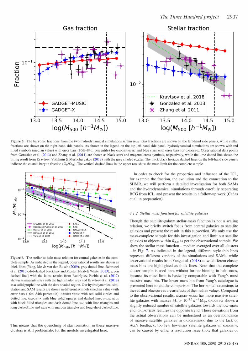
The Three Hundred project 2907

Figure 5. The baryonic fractions from the two hydrodynamical simulations within R500. Gas fractions are shown on the left-hand side panels, while stellarfractions are shown on the right-hand side panels. As shown in the legend on the top-left-hand side panel, hydrodynamical simulations are shown with redfilled symbols (median value) with error bars (16th–84th percentile) for GADGET-MUSIC and blue stars with error bars for GADGET-X. Observational data pointsfrom Gonzalez et al. (2013) and Zhang et al. (2011) are shown as black stars and magenta cross symbols, respectively, while the lime dotted line shows thefitting result from Kravtsov, Vikhlinin & Meshcheryakov (2018) with the grey shaded scatter. The thick black horizon dashed lines on the left-hand side panelsindicate the cosmic baryon fraction ("b/"m). The vertical dashed lines in the upper row show the mass limit for the complete sample.

Figure 6. The stellar-to-halo mass relation for central galaxies in the com-plete sample. As indicated in the legend, observational results are shown asthick lines [Yang, Mo & van den Bosch (2009), grey dotted line, Behrooziet al. (2013), dot-dashed black line and Moster, Naab & White (2013), greendashed line] with the latest results from Rodrıguez-Puebla et al. (2017)shown as magenta stars with the light shaded area and Kravtsov et al. (2018)as a solid purple line with the dark shaded region. Our hydrodynamical sim-ulation and SAM results are shown in different symbols (median value) witherror bars (16th–84th percentile): GADGET-MUSIC with red solid circles anddotted line; GADGET-X with blue solid squares and dashed line; GALACTICUS

with black filled triangles and dash-dotted line, SAG with lime triangles andlong dashed line and SAGE with maroon triangles and long-short dashed line.

This means that the quenching of star formation in these massiveclusters is still problematic for the models investigated here.

In order to check for the properties and influence of the ICL,for example the fraction, the evolution and the connection to theSHMR, we will perform a detailed investigation for both SAMsand the hydrodynamical simulations through carefully separatingBCG from ICL, and present the results in a follow-up work (Canaset al. in preparation).

4.1.2 Stellar mass function for satellite galaxies

Though the satellite-galaxy stellar-mass function is not a scalingrelation, we briefly switch focus from central galaxies to satellitegalaxies and present the result in this subsection. We only use themass-complete sample for this investigation and limit our satellitegalaxies to objects within R200 as per the observational sample. Weshow the stellar mass function – median averaged over all clusters– in Fig. 7. As indicated in the legend, different style thin linesrepresent different versions of the simulations and SAMs, whileobservational results from Yang et al. (2018) at two different clustermass bins are highlighted as thick lines. Note that the completecluster sample is used here without further binning in halo mass,because its mass limit is basically comparable with Yang’s mostmassive mass bin. The lower mass bin from Yang’s catalogue ispresented here to aid the comparison. The horizontal extensions tothe red and blue curves are artefacts of the median values. Comparedto the observational results, GADGET-MUSIC has more massive satel-lite galaxies with masses M∗ > 1011.5 h−1 M⊙. GADGET-X shows aslightly reduced number of satellite galaxies towards the low-massend. GALACTICUS features the opposite trend. These deviations fromthe actual observations can be understood as an overabundanceof massive satellite galaxies in GADGET-MUSIC due to the lack ofAGN feedback; too few low-mass satellite galaxies in GADGET-X

can be caused by either a resolution issue (note that galaxies of

MNRAS 480, 2898–2915 (2018)

Dow

nloaded from https://academ

ic.oup.com/m

nras/article-abstract/480/3/2898/5066184 by Konkoly Observatory user on 23 Septem

ber 2019

2908 W. Cui et al.

Figure 7. The median stellar mass function of satellite galaxies within themass-complete cluster sample. GADGET-MUSIC is shown with a red line withcircle symbols and GADGET-X with a blue line with square symbols. Thethree SAMs are presented by different lines: GALACTICUS as a black dashedline, SAG as a cyan dotted line, and SAGE as a magenta dot dashed line. Theyare compared with observational results from Yang et al. (2018), which areshown in thick black for halo mass range [1014.7 − 1015 h−1

0.72 M⊙] and thickgrey for halo mass range [1014.4 − 1014.7 h−1

0.72 M⊙], both lines include errorbars.

M∗ ≈ 1010 h−1 M⊙ only contain a few hundreds of stellar parti-cles due to the poor simulation resolution) or the striped/heatedgas due to the Wendland kernel and feedback; too many low-masssatellite galaxies in GALACTICUS is because of a surplus of orphangalaxies (see Table 2 in Knebe et al. 2018). SAG and SAGE seemnot to suffer from this problem due to their different treatmentof the orphan galaxy population. We refer to Pujol et al. (2017)for a detailed comparison of the orphan galaxies between differentSAMs. However, we note that the scatter across models seen hereis at the level found in previous comparisons of theoretically mod-elled galaxy stellar mass functions of galaxies (Knebe et al. 2015,2018).

4.1.3 Optical scaling relations

We continue to investigate the correlations between luminos-ity/magnitude, stellar mass, and colours by comparing our modelledgalaxies to the observational results from Yang et al. (2018). Weagain only use the galaxies from our mass-complete sample here.For a fair comparison to our theoretical data, we apply the samemass cut (M200 ≥ 6.42 × 1014 h−1 M⊙) to the group catalogue ofYang et al. (2018) and use all the satellites and central galaxieswith M∗ > 109 h−1 M⊙ in these selected groups (the same criteriaalso applied to our complete sample). The results can be viewed inFig. 8 where the top panel shows the luminosity–stellar mass rela-tion (based upon the SDSS-r band), the middle panel presents theg − r colour–magnitude (at SDSS-r band) relation, and the bottompanel shows the colour–colour relation with u − r versus r − i. Notethat the SAGE model does not provide luminosities ab initio and hashence been excluded from this plot. Similar to Fig. 5, the contoursare drawn at the same percentile density levels (16th, 50th, and84th) after a normalized 2D binning with the observational resultsshown as different colour-filled areas.

In the top panel, we recover a very tight correlation betweenluminosity and stellar mass with little variation between obser-

Figure 8. Top panel: the luminosity–stellar mass relation for all the galaxiesinside the clusters (using the SDSS-r band). As indicated in the legend,different symbols (median value) with error bars (16th − 84th percentile)are for different models and for the observational result from Yang et al.(2018), while the result from SAG is presented in cyan contours. The topsloping black line (shifted up by 0.5 dex) shows the slope 0.895 which fitsboth the models and the observational result. Middle panel: the colour–magnitude relation for the galaxies inside the clusters. Bottom panel: thecolour–colour relation for galaxies inside the clusters. The legend in themiddle panel distinguishes the colours for the models with different linestyles for both middle and bottom panels with the colour map is again fromYang et al. (2018).

MNRAS 480, 2898–2915 (2018)

Dow

nloaded from https://academ

ic.oup.com/m

nras/article-abstract/480/3/2898/5066184 by Konkoly Observatory user on 23 Septem

ber 2019

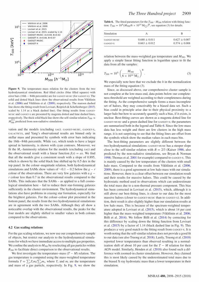
The Three Hundred project 2909

Figure 9. The temperature–mass relation for the clusters from the twohydrodynamical simulations. Red filled circles (blue filled squares) witherror bars (16th − 84th percentile) are for GADGET-MUSIC (for GADGET-X). Thesolid and dotted black lines show the observational results from Vikhlininet al. (2006) and Vikhlinin et al. (2009), respectively. The maroon dashedline shows the fitting result from Lovisari, Reiprich & Schellenberger (2015;scaled by 1.14 as a black dashed line). Our fitting results from GADGET-MUSIC and GADGET-X are presented by magenta dotted and lime dashed lines,respectively. The thick solid black line shows the self-similar relation T500 ∝M

2/3500 predicted from non-radiative simulations.

vation and the models (excluding SAG). GADGET-MUSIC, GADGET-X,GALACTICUS, and Yang’s observational results are binned only instellar mass and presented by symbols with error bars indicatingthe 16th−84th percentile. While SAG, which tends to have a largerspread in luminosity, is shown with cyan contours. Moreover, wefit the M∗–luminosity relation for the models (excluding SAG) andthe observational result with a linear function f(x) = ax. We findthat all the models give a consistent result with a slope of 0.895,which is shown by the solid black line shifted up by 0.5 dex in thetop panel. In the colour–magnitude relation, both hydrodynamicalsimulations and SAMs show values of ∼0.1 − 0.2 below the g − rcolour of the observations. There are very few galaxies with a g −r colour less than 0.7 in the observational results compared to theSAMs. This indicates that the SAMs – as applied to a full cosmo-logical simulation here – fail to reduce their star-forming galaxiessufficiently in the cluster environment. The hydrodynamical simu-lations also have problems in ceasing star formation, especially forthe brightest galaxies. For the colour–colour plot presented in thebottom panel, the results from the two hydrodynamical simulationsare in agreement with the two SAMs. Although they all show anoticeable overlap with the observational results, the peaks for thefour models are slightly shifted to smaller values in both colourscompared to the observations.

4.2 Gas scaling relations

For the gas scaling relations, we now use our comprehensive sampleof objects, but restrict our analysis to the hydrodynamical simula-tions for which we have immediate access to multiple gas properties.We confine the analysis to M500 by reselecting all gas particles withinR500 to facilitate direct comparison to the observational results.

We first investigate the temperature–mass (T − M) relation. Thegas temperature is computed using the mass-weighted temperatureformula T =

!iTimi/

!imi, where Ti and mi are the temperature

and mass of a gas particle, respectively. In Fig. 9, we show the

Table 6. The fitted parameters for the T500−M500 relation with fitting func-tion: T500 = 10A(M500/6 × 1014 M⊙)B, see equation (3) for details.

Simulation A B

GADGET-MUSIC 0.688 ± 0.011 0.627 ± 0.007GADGET-X 0.663 ± 0.012 0.574 ± 0.008

relation between the mass-weighted gas temperature and M500. Weapply a simple linear fitting function in logarithm space to fit thedata from all the samples:

T500 = 10A"

M500

6 × 1014 M⊙

#B

. (3)

We especially note here that we exclude the h in the normalizationmass of the fitting equation (3).

Since, as discussed above, our comprehensive cluster sample isnot complete at the low-mass end, data points below our complete-ness threshold are weighted according to their completeness duringthe fitting. As the comprehensive sample forms a mass-incompleteset of haloes, they may conceivably be a biased data set. Such abias could in principle arise due to their physical proximity to alarger halo but how to accurately quantify such a bias, if it exists, isunclear. Best-fitting curves are shown as a magenta dotted line forGADGET-MUSIC and a green dashed line for GADGET-X; the parametersare summarized both in the legend and Table 6. Since the low-massdata has less weight and there are few clusters in the high massrange, it is not surprising to see that the fitting lines are offset fromthe symbols which show the median values in each mass bin.

The best-fitting parameters are slightly different between thetwo hydrodynamical simulations: GADGET-MUSIC has a steeper slopeclose to the self-similar relation with B = 2/3 (Kaiser 1986, alsopredicted by the non-radiative simulations, see Bryan & Norman1998; Thomas et al. 2001 for example) compared to GADGET-X. Thisis mainly caused by the low temperature of the clusters with smallhalo mass. Compared to the results from Vikhlinin et al. (2006,2009), there is a good agreement at low halo mass with our simula-tions. However, there is a clear offset between our simulation resultand their results for massive haloes. This could be caused by thehydrostatic method used in observations which can underestimatethe total mass due to a non-thermal pressure component. This biashas been corrected in Lovisari et al. (2015), which, although it isstill above our best-fitting lines, is closer to our data for the mostmassive haloes (closer to GADGET-MUSIC than to GADGET-X). In addi-tion, their result is also slightly higher than our simulation results atlow halo mass. This is because of the spectrum-weighted temper-ature adopted in Lovisari et al. (2015), which is about 14 per centhigher than the mass-weighted temperature (Vikhlinin et al. 2006;Biffi et al. 2014). We follow Biffi et al. (2014) by correcting forthis difference by scaling down the fitting function from Lovisariet al. (2015) by a factor of 1.14 (black dashed line in Fig. 9). Thisproduces a very good match to the fitting result from GADGET-X. It isworth noting that the self-similar relation does not provide a good fitto our data (see also Truong et al. 2018). Lastly, Truong et al. (2018)reported lower temperatures than observed resulting in a normal-ization shift of about 10 per cent for the T − M relation for theirAGN model. Similarly, Henden et al. (2018) also found such a dif-ference with zoomed-in cluster simulations. However, they claimedthis is most likely caused by the underestimated total mass due tothe biased X-ray hydrostatic mass than a lower temperature in theirsimulation.

MNRAS 480, 2898–2915 (2018)

Dow

nloaded from https://academ

ic.oup.com/m

nras/article-abstract/480/3/2898/5066184 by Konkoly Observatory user on 23 Septem

ber 2019

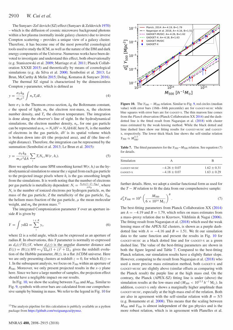
2910 W. Cui et al.

The Sunyaev-Zel’dovich (SZ) effect (Sunyaev & Zeldovich 1970)– which is the diffusion of cosmic microwave background photonswithin a hot plasma (normally inside galaxy clusters) due to inverseCompton scattering – provides a unique view of a galaxy cluster.Therefore, it has become one of the most powerful cosmologicaltools used to study the ICM, as well as the nature of the DM and darkenergy components of the Universe. Numerous works have been de-voted to investigate and understand this effect, both observationally(e.g. Staniszewski et al. 2009; Marriage et al. 2011; Planck Collab-oration XXXII 2015) and theoretically by means of cosmologicalsimulations (e.g. da Silva et al. 2000; Sembolini et al. 2013; LeBrun, McCarthy & Melin 2015; Dolag, Komatsu & Sunyaev 2016).

The thermal SZ signal is characterized by the dimensionlessCompton y-parameter, which is defined as

y = σT kB

mec2

$neTedl, (4)

here σ T is the Thomson cross-section, kB the Boltzmann constant,c the speed of light, me the electron rest-mass, ne the electronnumber density, and Te the electron temperature. The integrationis done along the observer’s line of sight. In the hydrodynamicalsimulations, the electron number density, ne, for one gas particlecan be represented as ne = Ne/dV = Ne/dA/dl, here Ne is the numberof electrons in the gas particle, dV is its spatial volume whichis broken down into dA (the projected area), and dl (the line-of-sight distance). Therefore, the integration can be represented by thesummation (Sembolini et al. 2013; Le Brun et al. 2015):

y = σT kB

mec2dA

%

i

TiNe,iW (r, hi). (5)

Here we applied the same SPH smoothing kernel W(r, hi) as the hy-drodynamical simulation to smear the y signal from each gas particleto the projected image pixels where hi is the gas smoothing lengthfrom the simulations. It is worth noting that the number of electronsper gas particle is metallicity dependent: Ni = Nemi(1−Z−YHe)

µmp, where

Ne is the number of ionized electrons per hydrogen particle, mi themass of the gas particle, Z the metallicity of the gas particle, YHe

the helium mass fraction of the gas particle, µ the mean molecularweight, and mp the proton mass.13

The integrated Comptonization parameter Y over an aperture in-side R is given by

Y =$

yd" =i ∈ R%

i

yi, (6)

where " is a solid angle, which can be expressed as an aperture ofradius R. In observations, this Y parameter is normally re-expressedas dA(z)2E(z)Y, where dA(z) is the angular diameter distance andE(z) = H (z)/H0 =

&"m(1 + z)3 + "# gives the redshift evolu-

tion of the Hubble parameter, H(z), in a flat #CDM universe. Herewe are only presenting clusters at redshift z = 0, for which E(z) =1. In the subsequent analysis, we focus on Y500 within an aperture ofR500. Moreover, we only present projected results in the x–y planehere. Since we have a large number of samples, the projection effectshould have a negligible impact on our results.

In Fig. 10, we show the scaling between Y500 and M500. Similar toFig. 9, symbols with error bars are calculated from our comprehen-sive sample by binning in mass. We refer to the legend in Fig. 10 for

13The analysis pipeline for this calculation is publicly available as a pythonpackage from https://github.com/weiguangcui/pymsz.

Figure 10. The Y500 − M500 relation. Similar to Fig. 9, red circles (medianvalue) with error bars (16th−84th percentile) are for GADGET-MUSIC whileblue squares with error bars are for GADGET-X. The thin maroon line comesfrom the Planck observation (Planck Collaboration XX 2014) and the dash-dotted line is the fitted result from Nagarajan et al. (2018) with clustermass estimated by the weak-lensing method. While the black dotted andlime dashed lines show our fitting results for GADGET-MUSIC and GADGET-X, respectively. The lower thick black line shows the self-similar relationY500 ∝ M

5/3500 .

Table 7. The fitted parameters for the Y500−M500 relation. See equation (7)for details.

Simulation A B

GADGET-MUSIC −4.26 ± 0.07 1.62 ± 0.31GADGET-X −4.18 ± 0.07 1.63 ± 0.29

further details. Here, we adopt a similar functional form as used forthe T − M relation to fit the data from our comprehensive sample:

d2AY500 = 10A

"M500

6 × 1014 M⊙

#B

. (7)

The best-fitting parameters from Planck Collaboration XX (2014)are A = −4.19 and B = 1.79, which relies on mass estimates froma mass–proxy relation due to Kravtsov, Vikhlinin & Nagai (2006).The fitting result from Nagarajan et al. (2018) which used the weaklensing mass of the APEX-SZ clusters, is shown as a purple dash-dotted line with A = −4.16 and B = 1.51. We fit our simulationdata to the same function and present the results in Fig. 10 forGADGET-MUSIC as a black dotted line and for GADGET-X as a greendashed line. The value of the best-fitting parameters are shown inboth the figure legend and Table 7. Compared to the best-fittingPlanck relation, our simulation results have a slightly flatter slope.However, comparing to the result from Nagarajan et al. (2018) whoused a more precise mass estimation method, both GADGET-X andGADGET-MUSIC are slightly above (similar offsets as comparing withthe Planck result) the purple line at the high mass end. On thecontrary, the Planck (APEX-SZ) fitting line is under (above) thesimulation results at the low-mass end (M500 < 1013.5 h−1 M⊙). Inaddition, GADGET-X only shows a marginally higher amplitude thanGADGET-MUSIC, especially at the high-mass end of the relation. Bothare also in agreement with the self-similar relation with B = 5/3(e.g. Bonamente et al. 2008). This means that the scaling betweenM500 and Y500 is almost independent of the gas physics and is themore robust relation, which is in agreement with Planelles et al.

MNRAS 480, 2898–2915 (2018)

Dow

nloaded from https://academ

ic.oup.com/m

nras/article-abstract/480/3/2898/5066184 by Konkoly Observatory user on 23 Septem

ber 2019

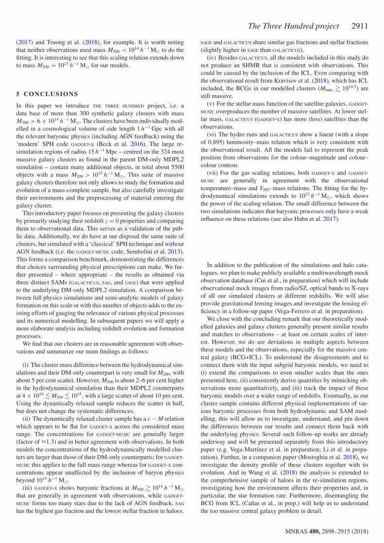
The Three Hundred project 2911

(2017) and Truong et al. (2018), for example. It is worth notingthat neither observations used mass M500 < 1014 h−1 M⊙ to do thefitting. It is interesting to see that this scaling relation extends downto mass M500 = 1013 h−1 M⊙ for our models.

5 C O N C L U S I O N S

In this paper we introduce THE THREE HUNDRED project, i.e. adata base of more than 300 synthetic galaxy clusters with massM200 > 6 × 1014 h−1 M⊙. The clusters have been individually mod-elled in a cosmological volume of side length 1 h−1 Gpc with allthe relevant baryonic physics (including AGN feedback) using the‘modern’ SPH code GADGET-X (Beck et al. 2016). The large re-simulation regions of radius 15 h−1 Mpc – centred on the 324 mostmassive galaxy clusters as found in the parent DM-only MDPL2simulation – contain many additional objects, in total about 5500objects with a mass M200 > 1013 h−1 M⊙. This suite of massivegalaxy clusters therefore not only allows to study the formation andevolution of a mass-complete sample, but also carefully investigatetheir environments and the preprocessing of material entering thegalaxy cluster.

This introductory paper focuses on presenting the galaxy clustersby primarily studying their redshift z = 0 properties and comparingthem to observational data. This serves as a validation of the pub-lic data. Additionally, we do have at our disposal the same suite ofclusters, but simulated with a ‘classical’ SPH technique and withoutAGN feedback (i.e. the GADGET-MUSIC code, Sembolini et al. 2013).This forms a comparison benchmark, demonstrating the differencesthat choices surrounding physical prescriptions can make. We fur-ther presented – where appropriate – the results as obtained viathree distinct SAMs (GALACTICUS, SAG, and SAGE) that were appliedto the underlying DM-only MDPL2 simulation. A comparison be-tween full physics simulations and semi-analytic models of galaxyformation on this scale or with this number of objects adds to the ex-isting efforts of gauging the relevance of various physical processesand its numerical modelling. In subsequent papers we will apply amore elaborate analysis including redshift evolution and formationprocesses.

We find that our clusters are in reasonable agreement with obser-vations and summarize our main findings as follows:

(i) The cluster mass difference between the hydrodynamical sim-ulations and their DM-only counterpart is very small for M200, withabout 5 per cent scatter. However, M500 is about 2–6 per cent higherin the hydrodynamical simulation than their MDPL2 counterpartsat 4 × 1014 " M500 " 1015, with a large scatter of about 10 per cent.Using the dynamically relaxed sample reduces the scatter in half,but does not change the systematic differences.

(ii) The dynamically relaxed cluster sample has a c − M relationwhich appears to be flat for GADGET-X across the considered massrange. The concentrations for GADGET-MUSIC are generally larger(factor of ≈ 1.3) and in better agreement with observations. In bothmodels the concentrations of the hydrodynamically modelled clus-ters are larger than those of their DM-only counterparts; for GADGET-MUSIC this applies to the full mass range whereas for GADGET-X con-centrations appear unaffected by the inclusion of baryon physicsbeyond 1015 h−1 M⊙.

(iii) GADGET-X shows baryonic fractions at M500 # 1014 h−1 M⊙that are generally in agreement with observations, while GADGET-MUSIC forms too many stars due to the lack of AGN feedback. SAG

has the highest gas fraction and the lowest stellar fraction in haloes.

SAGE and GALACTICUS share similar gas fractions and stellar fractions(slightly higher in SAGE than GALACTICUS).

(iv) Besides GALACTICUS, all the models included in this study donot produce an SHMR that is consistent with observations. Thiscould be caused by the inclusion of the ICL. Even comparing withthe observational result from Kravtsov et al. (2018), which has ICLincluded, the BCGs in our modelled clusters (Mhalo # 1014.5) arestill massive.

(v) For the stellar mass function of the satellite galaxies, GADGET-MUSIC overproduces the number of massive satellites. At lower stel-lar mass, GALACTICUS (GADGET-X) has more (less) satellites than theobservations.

(vi) The hydro runs and GALACTICUS show a linear (with a slopeof 0.895) luminosity–mass relation which is very consistent withthe observational result. All the models fail to represent the peakposition from observations for the colour–magnitude and colour–colour contour.

(vii) For the gas scaling relations, both GADGET-X and GADGET-MUSIC are generally in agreement with the observationaltemperature–mass and Y500–mass relations. The fitting for the hy-drodynamical simulations extends to 1013 h−1 M⊙, which showsthe power of the scaling relation. The small difference between thetwo simulations indicates that baryonic processes only have a weakinfluence on these relations (see also Hahn et al. 2017).

In addition to the publication of the simulations and halo cata-logues, we plan to make publicly available a multiwavelength mockobservation database (Cui et al., in preparation) which will includeobservational mock images from radio/SZ, optical bands to X-raysof all our simulated clusters at different redshifts. We will alsoprovide gravitational lensing images and investigate the lensing ef-ficiency in a follow-up paper (Vega-Ferrero et al. in preparation).

We close with the concluding remark that our theoretically mod-elled galaxies and galaxy clusters generally present similar resultsand matches to observations – at least on certain scales of inter-est. However, we do see deviations in multiple aspects betweenthese models and the observations, especially for the massive cen-tral galaxy (BCG+ICL). To understand the disagreements and toconnect them with the input subgrid baryonic models, we need to(i) extend the comparisons to even smaller scales than the onespresented here, (ii) consistently derive quantities by mimicking ob-servations more quantitatively, and (iii) track the impact of thesebaryonic models over a wider range of redshifts. Eventually, as ourcluster sample contains different physical implementations of var-ious baryonic processes from both hydrodynamic and SAM mod-elling, this will allow us to investigate, understand, and pin downthe differences between our results and connect them back withthe underlying physics. Several such follow-up works are alreadyunderway and will be presented separately from this introductorypaper (e.g. Vega-Martınez et al. in preparation; Li et al. in prepa-ration). Further, in a companion paper (Mostoghiu et al. 2018), weinvestigate the density profile of these clusters together with itsevolution. And in Wang et al. (2018) the analysis is extended tothe comprehensive sample of haloes in the re-simulation regions,investigating how the environment affects their properties and, inparticular, the star formation rate. Furthermore, disentangling theBCG from ICL (Canas et al., in prep.) will help us to understandthe too massive central galaxy problem in detail.

MNRAS 480, 2898–2915 (2018)

Dow

nloaded from https://academ

ic.oup.com/m

nras/article-abstract/480/3/2898/5066184 by Konkoly Observatory user on 23 Septem

ber 2019

2912 W. Cui et al.

ACKNOWLEDGEMENTS

The work has received financial support from the European Union’sHorizon 2020 Research and Innovation programme under theMarie Sklodowskaw-Curie grant agreement number 734374, i.e.the LACEGAL project.14 The workshop where this work has beenfinished was sponsored in part by the Higgs Centre for TheoreticalPhysics at the University of Edinburgh.

The authors would like to thank The Red Espanola de Supercom-putacion for granting us computing time at the MareNostrum Su-percomputer of the BSC-CNS where most of the cluster simulationshave been performed. The MDPL2 simulation has been performedat LRZ Munich within the project pr87yi. The CosmoSim database(https://www.cosmosim.org) is a service by the Leibniz Institute forAstrophysics Potsdam (AIP). Part of the computations with GADGET-X have also been performed at the ‘Leibniz-Rechenzentrum’ withCPU time assigned to the Project ‘pr83li’.

This work has made extensive use of the PYTHON packages –IPYTHON with its Jupyter notebook (Perez & Granger 2007), NUMPY

(van der Walt, Colbert & Varoquaux 2011), and SCIPY (Oliphant2007; Millman & Aivazis 2011). All the figures in this paper areplotted using the python MATPLOTLIB package (Hunter 2007). Thisresearch has made use of NASA’s Astrophysics Data System andthe arXiv preprint server.

WC, AK, GY, and RM are supported by the Ministerio deEconomıa y Competitividad and the Fondo Europeo de Desar-rollo Regional (MINECO/FEDER, UE) in Spain through grantAYA2015-63810-P. WC further thanks TaiLai Cui (!!!) for allthe joys. AK is also supported by the Spanish Red Consolider Mul-tiDark FPA2017-90566-REDC and further thanks Krog for makingthe days counts. CP acknowledges the Australia Research Coun-cil (ARC) Centre of Excellence (CoE) ASTRO 3D through projectnumber CE170100013. PJE is supported by the ARC CoE ASTRO3D through project number CE170100013. SB acknowledged fi-nancial support from PRIN-MIUR grant 2015W7KAWC, the agree-ment ASI-INAF n.2017-14-H.0, the INFN INDARK grant, the EUH2020 Research and Innovation Programme under the ExaNeStproject (Grant Agreement No. 671553). ER acknowledges the Ex-aNeSt and Euro Exa projects, funded by the European Union’sHorizon 2020 research and innovation programme under grantagreement No. 671553 and No. 754337 and financial contribu-tion from the agreement ASI-INAF n.2017-14-H.0. DS’ fellowshipis funded by the Spanish Ministry of Economy and Competitive-ness (MINECO) under the 2014 Severo Ochoa Predoctoral TrainingProgramme. J.V-F acknowledges the hospitality of the Physics &Astronomy Department at the University of Pennsylvania for host-ing him during the preparation of this work. YW is supported bythe national science foundation of China (No. 11643005). XY issupported by the National Key Basic Research Program of China(No. 2015CB857002), national science foundation of China (No.11233005, 11621303). JTA acknowledges support from a postgrad-uate award from STFC. SAC acknowledges funding from Con-sejo Nacional de Investigaciones Cientıficas y Tecnicas (CON-ICET, PIP-0387), Agencia Nacional de Promocion Cientıfica y Tec-nologica (ANPCyT, PICT-2013-0317), and Universidad Nacionalde La Plata(G11-124), Argentina. CVM acknowledges CONICET,Argentina, for their supporting fellowships. ASB, GC, and MDPare supported by Sapienza University of Rome-Progetti di RicercaAnno 2016. ASB also acknowledges funding from Sapienza Uni-

14https://cordis.europa.eu/project/rcn/207630 en.html

versita di Roma under minor grant Progetti per Avvio alla RicercaAnno 2017, prot. AR11715C82402BC7. RC is supported by theMERAC foundation postdoctoral grant awarded to Claudia Lagosand by the Consejo Nacional de Ciencia y Tecnologıa CONACYTCVU 520137 Scholar 290609 Overseas Scholarship 438594. SEacknowledges financial contribution from the contracts NARO15ASI-INAF I/037/12/0, ASI 2015-046-R.0, and ASI-INAF n.2017-14-H.0. SEN is a member of the Carrera del Investigador Cientıficoof CONICET. SP is supported by the Fundamental Research Pro-gram of Presidium of the RAS #28. JS acknowledges support fromthe “Centre National d’etudes spatiales” (CNES) postdoctoral fel-lowship program as well as from the “l’Oreal-UNESCO pour lesfemmes et la Science” fellowship program.

R E F E R E NCES

Andersson K. et al., 2011, ApJ, 738, 48Arthur J. et al., 2017, MNRAS, 464, 2027Bahe Y. M. et al., 2017, MNRAS, 470, 4186Barnes D. J., Kay S. T., Henson M. A., McCarthy I. G., Schaye J., Jenkins

A., 2017a, MNRAS, 465, 213Barnes D. J. et al., 2017b, MNRAS, 471, 1088Beck A. M. et al., 2016, MNRAS, 455, 2110Behroozi P. et al., 2015, MNRAS, 454, 3020Behroozi P. S., Wechsler R. H., Wu H.-Y., 2013, ApJ, 762, 109Benitez-Llambay A., 2015, py-sphviewer: Py-SPHViewer v1.0.0Benson A. J., 2012, New Astron., 17, 175Bernyk M. et al., 2016, ApJS, 223, 9Biffi V., Sembolini F., De Petris M., Valdarnini R., Yepes G., Gottlober S.,

2014, MNRAS, 439, 588Biffi V. et al., 2016, ApJ, 827, 112Biviano A. et al., 2017, A&A, 607, A81Bocquet S., Saro A., Dolag K., Mohr J. J., 2016, MNRAS, 456, 2361Bonamente M., Joy M., LaRoque S. J., Carlstrom J. E., Nagai D., Marrone

D. P., 2008, ApJ, 675, 106Bryan G. L., Norman M. L., 1998, ApJ, 495, 80Bullock J. S., Kolatt T. S., Sigad Y., Somerville R. S., Kravtsov A. V., Klypin

A. A., Primack J. R., Dekel A., 2001, MNRAS, 321, 559Carlesi E., Knebe A., Yepes G., Gottlober S., Jimenez J. B., Maroto A. L.,

2012, MNRAS, 424, 699Chabrier G., 2003, PASP, 115, 763Chiu I. et al., 2018, MNRAS, 478, 3072Cora S. A. et al., 2018, MNRAS, 479, 2Croton D. J. et al., 2016, ApJS, 222, 22Cui W., Zhang Y., 2017, Trends in Modern Cosmology, IntechOpen, Lon-

don, UK, p. 22, 978-953-51-5426-6.Cui W., Springel V., Yang X., De Lucia G., Borgani S., 2011, MNRAS, 416,

2997Cui W., Borgani S., Dolag K., Murante G., Tornatore L., 2012, MNRAS,

423, 2279Cui W. et al., 2014a, MNRAS, 437, 816Cui W., Borgani S., Murante G., 2014b, MNRAS, 441, 1769Cui W. et al., 2016a, MNRAS, 456, 2566Cui W. et al., 2016b, MNRAS, 458, 4052Cui W., Power C., Borgani S., Knebe A., Lewis G. F., Murante G., Poole G.

B., 2017, MNRAS, 464, 2502da Silva A. C., Barbosa D., Liddle A. R., Thomas P. A., 2000, MNRAS,

317, 37Devriendt J. E. G., Guiderdoni B., Sadat R., 1999, A&A, 350, 381Dolag K., Bartelmann M., Perrotta F., Baccigalupi C., Moscardini L.,

Meneghetti M., Tormen G., 2004, A&A, 416, 853Dolag K., Komatsu E., Sunyaev R., 2016, MNRAS, 463, 1797Eckert D. et al., 2016, A&A, 592, A12Elahi P. J. et al., 2016, MNRAS, 458, 1096Evrard A. E., Metzler C. A., Navarro J. F., 1996, ApJ, 469, 494Gonzalez A. H., Zaritsky D., Zabludoff A. I., 2007, ApJ, 666, 147

MNRAS 480, 2898–2915 (2018)

Dow

nloaded from https://academ

ic.oup.com/m

nras/article-abstract/480/3/2898/5066184 by Konkoly Observatory user on 23 Septem

ber 2019

The Three Hundred project 2913

Gonzalez A. H., Sivanandam S., Zabludoff A. I., Zaritsky D., 2013, ApJ,778, 14

Groener A. M., Goldberg D. M., Sereno M., 2016, MNRAS, 455, 892Guo Q., White S., Li C., Boylan-Kolchin M., 2010, MNRAS, 404, 1111Guo Q. et al., 2016, MNRAS, 461, 3457Haardt F., Madau P., 1996, ApJ, 461, 20Haardt F., Madau P., 2001, in Neumann D. M., Tran J. T. V., eds, Clusters

of Galaxies and the High Redshift Universe Observed in X-rays, XXIstMoriond astrophysics meeting, CEA, Savoie, France

Hahn O., Martizzi D., Wu H.-Y., Evrard A. E., Teyssier R., Wechsler R. H.,2017, MNRAS, 470, 166

Henden N. A., Puchwein E., Shen S., Sijacki D., 2018, MNRAS, 479,5385

Hunter J. D., 2007, Comput. Sci. Eng., 9, 90Kaiser N., 1986, MNRAS, 222, 323Kennicutt R. C., Jr, 1998, in Gilmore G., Howell D., eds, ASP Conf. Ser., Vol.

142, The Stellar Initial Mass Function (38th Herstmonceux Conference),Astron. Soc. Pac., San Francisco. p. 1

Klypin A., Yepes G., Gottlober S., Prada F., Heß S., 2016, MNRAS, 457,4340

Knebe A., Draganova N., Power C., Yepes G., Hoffman Y., Gottlober S.,Gibson B. K., 2008, MNRAS, 386, L52

Knebe A. et al., 2011, MNRAS, 415, 2293Knebe A. et al., 2013, MNRAS, 435, 1618Knebe A. et al., 2015, MNRAS, 451, 4029Knebe A. et al., 2018, MNRAS, 475, 2936Knollmann S. R., Knebe A., 2009, ApJS, 182, 608Kravtsov A. V., Vikhlinin A., Nagai D., 2006, ApJ, 650, 128Kravtsov A. V., Vikhlinin A. A., Meshcheryakov A. V., 2018, Astron. Lett.,

44, 8Lagana T. F., Martinet N., Durret F., Lima Neto G. B., Maughan B., Zhang

Y.-Y., 2013, A&A, 555, A66Le Brun A. M. C., McCarthy I. G., Schaye J., Ponman T. J., 2014, MNRAS,

441, 1270Le Brun A. M. C., McCarthy I. G., Melin J.-B., 2015, MNRAS, 451, 3868Lin Y.-T., Mohr J. J., Stanford S. A., 2004, ApJ, 610, 745Lovisari L., Reiprich T. H., Schellenberger G., 2015, A&A, 573, A118Mantz A. B., Allen S. W., Morris R. G., Schmidt R. W., von der Linden A.,

Urban O., 2015, MNRAS, 449, 199Mantz A. B., Allen S. W., Morris R. G., 2016, MNRAS, 462, 681Marriage T. A. et al., 2011, ApJ, 737, 61McCarthy I. G., Schaye J., Bird S., Le Brun A. M. C., 2017, MNRAS, 465,

2936Merten J. et al., 2015, ApJ, 806, 4Millman K. J., Aivazis M., 2011, Comput. Sci. Eng., 13, 9Monaco P., Benson A. J., De Lucia G., Fontanot F., Borgani S., Boylan-

Kolchin M., 2014, MNRAS, 441, 2058Moster B. P., Naab T., White S. D. M., 2013, MNRAS, 428, 3121Mostoghiu R., Knebe A., Cui W., Pearce F. R., Yepes G., Power C., Dave

R., Arth A., 2018, MNRAS, in reviewNagarajan A. et al., 2018, MNRAS tmp, 1811, preprint (arXiv:1804.03671)Navarro J. F., Frenk C. S., White S. D. M., 1997, ApJ, 490, 493Neto A. F. et al., 2007, MNRAS, 381, 1450Okabe N., Smith G. P., 2016, MNRAS, 461, 3794Oliphant T. E., 2007, Comput. Sci. Eng., 9, 10Perez F., Granger B. E., 2007, Comput. Sci. Eng., 9, 21Pillepich A. et al., 2018, MNRAS, 475, 648Planck Collaboration XX, 2014, A&A, 571, A20Planck Collaboration XXXII, 2015, A&A, 581, A14Planck Collaboration XIII, 2016, A&A, 594, A13Planelles S., Borgani S., Dolag K., Ettori S., Fabjan D., Murante G., Torna-

tore L., 2013, MNRAS, 431, 1487Planelles S. et al., 2017, MNRAS, 467, 3827Power C., Knebe A., Knollmann S. R., 2012, MNRAS, 419, 1576Puchwein E., Springel V., Sijacki D., Dolag K., 2010, MNRAS, 406, 936Pujol A. et al., 2017, MNRAS, 469, 749Ragone-Figueroa C., Granato G. L., Murante G., Borgani S., Cui W., 2013,

MNRAS, 436, 1750

Ragone-Figueroa C., Granato G. L., Ferraro M. E., Murante G., Biffi V.,Borgani S., Planelles S., Rasia E., 2018, MNRAS, 479, 1125

Rasia E., Borgani S., Ettori S., Mazzotta P., Meneghetti M., 2013, ApJ, 776,39

Reiprich T. H., Bohringer H., 2002, ApJ, 567, 716Rodrıguez-Puebla A., Primack J. R., Avila-Reese V., Faber S. M., 2017,

MNRAS, 470, 651Salpeter E. E., 1955, ApJ, 121, 161Saro A., De Lucia G., Borgani S., Dolag K., 2010, MNRAS, 406, 729Sartoris B. et al., 2016, MNRAS, 459, 1764Schaller M. et al., 2015a, MNRAS, 451, 1247Schaller M. et al., 2015b, MNRAS, 452, 343Sembolini F., Yepes G., De Petris M., Gottlober S., Lamagna L., Comis B.,

2013, MNRAS, 429, 323Sembolini F. et al., 2016a, MNRAS, 457, 4063Sembolini F. et al., 2016b, MNRAS, 459, 2973Springel V., 2005, MNRAS, 364, 1105Springel V., Hernquist L., 2003, MNRAS, 339, 289Staniszewski Z. et al., 2009, ApJ, 701, 32Steinborn L. K., Dolag K., Hirschmann M., Prieto M. A., Remus R.-S.,

2015, MNRAS, 448, 1504Sunyaev R. A., Zeldovich Y. B., 1970, Ap&SS, 7, 3Thomas P. A., Muanwong O., Pearce F. R., Couchman H. M. P., Edge A.

C., Jenkins A., Onuora L., 2001, MNRAS, 324, 450Tornatore L., Borgani S., Dolag K., Matteucci F., 2007, MNRAS, 382, 1050Truong N. et al., 2018, MNRAS, 474, 4089van der Walt S., Colbert S. C., Varoquaux G., 2011, Comput. Sci. Eng., 13,

22Vikhlinin A., Kravtsov A., Forman W., Jones C., Markevitch M., Murray S.

S., Van Speybroeck L., 2006, ApJ, 640, 691Vikhlinin A. et al., 2009, ApJ, 692, 1033Wang Y. et al., 2018, ApJ, in reviewWiersma R. P. C., Schaye J., Smith B. D., 2009, MNRAS, 393, 99Wu H.-Y., Evrard A. E., Hahn O., Martizzi D., Teyssier R., Wechsler R. H.,

2015, MNRAS, 452, 1982Yang X., Mo H. J., van den Bosch F. C., 2009, ApJ, 695, 900Yang X., Mo H. J., van den Bosch F. C., Zhang Y., Han J., 2012, ApJ, 752,

41Yang X. et al., 2018, ApJ, 860, 30Yepes G., Kates R., Khokhlov A., Klypin A., 1997, MNRAS, 284, 235Zhang Y.-Y., Lagana T. F., Pierini D., Puchwein E., Schneider P., Reiprich

T. H., 2011, A&A, 535, A78Zhao D. H., Mo H. J., Jing Y. P., Borner G., 2003a, MNRAS, 339, 12Zhao D. H., Jing Y. P., Mo H. J., Borner G., 2003b, ApJ, 597, L9Zibetti S., White S. D. M., Schneider D. P., Brinkmann J., 2005, MNRAS,

358, 949

A PPEN D I X: E VO L U T I ON OF TH E H ALO MASSF U N C T I O N

Our 30 h−1 Mpc diameter re-simulated regions contain many moreobjects in addition to the central clusters. While there are lots ofhaloes in the region that surrounds the central cluster there would bemany, many more similar haloes in the full volume. It is thereforeimportant to understand the completeness of our comprehensivesample. Here, completeness refers to the total number of haloesabove a given mass within a certain cosmological volume. Themass-complete sample in our hydrodynamic simulations is givenby Nhydro(> MX) ≥ NMDPL2(> MX). Here N is the total numberof haloes above a certain mass MX with X is the chosen massoverdensity e.g. 200. i.e. this is the mass above which our samplecontains every cluster in the full volume. Below this mass somehaloes have not been captured by our re-simulation procedure.

In Fig. A1, we show the cumulative halo mass functions for thetwo mass definitions M200 (left-hand side panel) and M500 (right-hand side panel) as derived from MDPL2 (solid black lines), GADGET-

MNRAS 480, 2898–2915 (2018)

Dow

nloaded from https://academ

ic.oup.com/m

nras/article-abstract/480/3/2898/5066184 by Konkoly Observatory user on 23 Septem

ber 2019

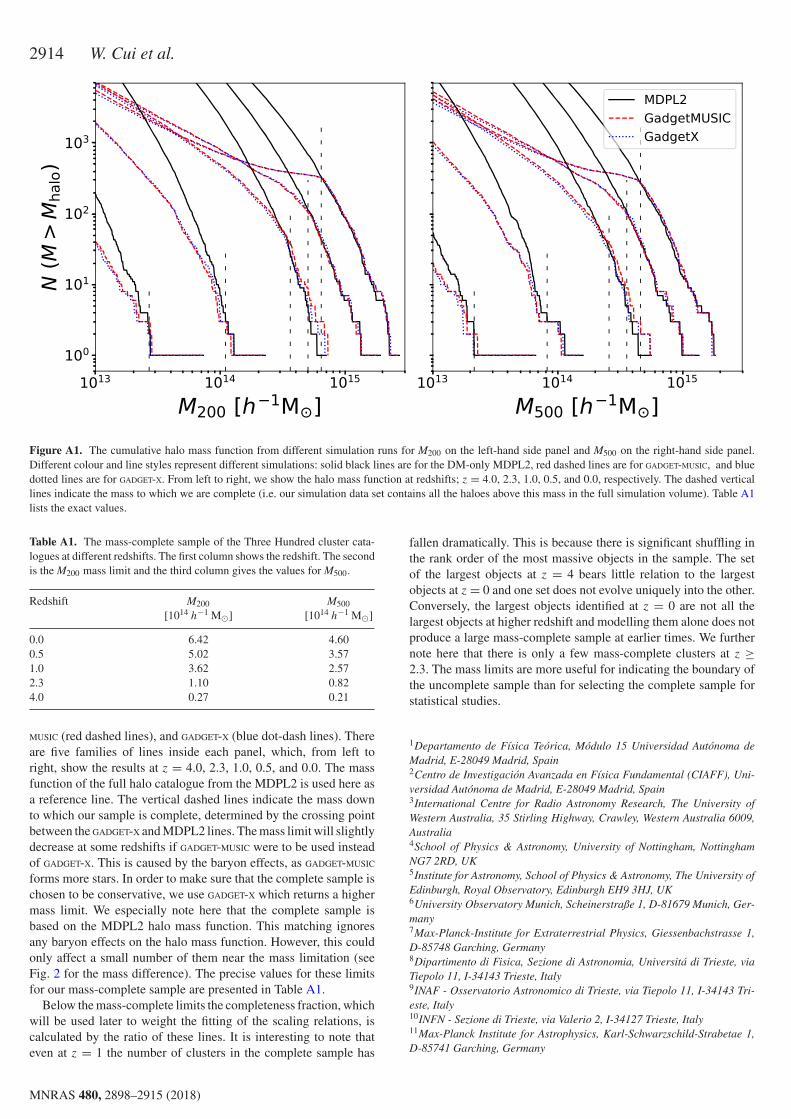
2914 W. Cui et al.

Figure A1. The cumulative halo mass function from different simulation runs for M200 on the left-hand side panel and M500 on the right-hand side panel.Different colour and line styles represent different simulations: solid black lines are for the DM-only MDPL2, red dashed lines are for GADGET-MUSIC, and bluedotted lines are for GADGET-X. From left to right, we show the halo mass function at redshifts; z = 4.0, 2.3, 1.0, 0.5, and 0.0, respectively. The dashed verticallines indicate the mass to which we are complete (i.e. our simulation data set contains all the haloes above this mass in the full simulation volume). Table A1lists the exact values.

Table A1. The mass-complete sample of the Three Hundred cluster cata-logues at different redshifts. The first column shows the redshift. The secondis the M200 mass limit and the third column gives the values for M500.

Redshift M200 M500[1014 h−1 M⊙] [1014 h−1 M⊙]

0.0 6.42 4.600.5 5.02 3.571.0 3.62 2.572.3 1.10 0.824.0 0.27 0.21

MUSIC (red dashed lines), and GADGET-X (blue dot-dash lines). Thereare five families of lines inside each panel, which, from left toright, show the results at z = 4.0, 2.3, 1.0, 0.5, and 0.0. The massfunction of the full halo catalogue from the MDPL2 is used here asa reference line. The vertical dashed lines indicate the mass downto which our sample is complete, determined by the crossing pointbetween the GADGET-X and MDPL2 lines. The mass limit will slightlydecrease at some redshifts if GADGET-MUSIC were to be used insteadof GADGET-X. This is caused by the baryon effects, as GADGET-MUSIC

forms more stars. In order to make sure that the complete sample ischosen to be conservative, we use GADGET-X which returns a highermass limit. We especially note here that the complete sample isbased on the MDPL2 halo mass function. This matching ignoresany baryon effects on the halo mass function. However, this couldonly affect a small number of them near the mass limitation (seeFig. 2 for the mass difference). The precise values for these limitsfor our mass-complete sample are presented in Table A1.

Below the mass-complete limits the completeness fraction, whichwill be used later to weight the fitting of the scaling relations, iscalculated by the ratio of these lines. It is interesting to note thateven at z = 1 the number of clusters in the complete sample has

fallen dramatically. This is because there is significant shuffling inthe rank order of the most massive objects in the sample. The setof the largest objects at z = 4 bears little relation to the largestobjects at z = 0 and one set does not evolve uniquely into the other.Conversely, the largest objects identified at z = 0 are not all thelargest objects at higher redshift and modelling them alone does notproduce a large mass-complete sample at earlier times. We furthernote here that there is only a few mass-complete clusters at z ≥2.3. The mass limits are more useful for indicating the boundary ofthe uncomplete sample than for selecting the complete sample forstatistical studies.

1Departamento de Fısica Teorica, Modulo 15 Universidad Autonoma deMadrid, E-28049 Madrid, Spain2Centro de Investigacion Avanzada en Fısica Fundamental (CIAFF), Uni-versidad Autonoma de Madrid, E-28049 Madrid, Spain3International Centre for Radio Astronomy Research, The University ofWestern Australia, 35 Stirling Highway, Crawley, Western Australia 6009,Australia4School of Physics & Astronomy, University of Nottingham, NottinghamNG7 2RD, UK5Institute for Astronomy, School of Physics & Astronomy, The University ofEdinburgh, Royal Observatory, Edinburgh EH9 3HJ, UK6University Observatory Munich, Scheinerstraße 1, D-81679 Munich, Ger-many7Max-Planck-Institute for Extraterrestrial Physics, Giessenbachstrasse 1,D-85748 Garching, Germany8Dipartimento di Fisica, Sezione di Astronomia, Universita di Trieste, viaTiepolo 11, I-34143 Trieste, Italy9INAF - Osservatorio Astronomico di Trieste, via Tiepolo 11, I-34143 Tri-este, Italy10INFN - Sezione di Trieste, via Valerio 2, I-34127 Trieste, Italy11Max-Planck Institute for Astrophysics, Karl-Schwarzschild-Strabetae 1,D-85741 Garching, Germany

MNRAS 480, 2898–2915 (2018)

Dow

nloaded from https://academ

ic.oup.com/m

nras/article-abstract/480/3/2898/5066184 by Konkoly Observatory user on 23 Septem

ber 2019

The Three Hundred project 2915

12Instituto de Fısica Teorica, (UAM/CSIC), Universidad Autonoma deMadrid, Cantoblanco, E-28049 Madrid, Spain13IFCA, Instituto de Fısica de Cantabria (UC-CSIC), Av. de Los Castross/n, E-39005 Santander, Spain14School of Physics and Astronomy, Sun Yat-sen University, 519082 Zhuhai,China15Department of Astronomy, Shanghai Key Laboratory for Particle Physicsand Cosmology, Shanghai Jiao Tong University, Shanghai 200240, China16IFSA Collaborative Innovation Center, and Tsung-Dao Lee Institute,Shanghai Jiao Tong University, Shanghai 200240, China17Carnegie Observatories, 813 Santa Barbara Street, Pasadena, CA 91101,USA18Instituto de Astrofısica de La Plata (CCT La Plata, CONICET, UNLP),Paseo del Bosque s/n, B1900FWA, La Plata, Argentina19Facultad de Ciencias Astronomicas y Geofısicas, Universidad Nacionalde La Plata, Paseo del Bosque s/n, B1900FWA, La Plata, Argentina20Centre for Astrophysics and Supercomputing, Swinburne University ofTechnology, Hawthorn, Victoria 3122, Australia21Department of Physics, Sapienza Universita di Roma, p.le Aldo Moro 5,I-00185 Rome, Italy22Dipartimento di Fisica, Universita di Roma Tor Vergata, via della RicercaScientifica 1, I-00133 Roma, Italy23South African Astronomical Observatory, PO Box 9, Observatory, CapeTown 7935, South Africa

24Department of Physics and Astronomy, University of the Western Cape,Cape Town 7535, South Africa25INFN - Sezione di Roma, P.le A. Moro 2, I-00185 Roma, Italy26Dipartimento di Fisica - Universita degli Studi di Torino, Via Pietro Giuria,1, I-10125 Torino, Italy27INAF, Osservatorio di Astrofisica e Scienza dello Spazio, via Pietro Gobetti93/3, I-40129 Bologna, Italy28INFN, Sezione di Bologna, viale Berti Pichat 6/2, I-40127 Bologna, Italy29Leibniz-Institut fur Astrophysik, D-14482 Potsdam, Germany30Instituto de Astronomıa y Fısica del Espacio (IAFE, CONICET-UBA), CC67, Suc. 28, 1428, Buenos Aires, Argentina31Facultad de Ciencias Exactas y Naturales (FCEyN), Universidad deBuenos Aires (UBA), 1053, Buenos Aires, Argentina32Department of Astronomy & Astrophysics, University of Toronto, Toronto,Canada33Astro Space Centre of Lebedev Physical Institute, Russian Academy ofSciences, Profsoyuznaja 84/32, 117997 Moscow, Russia34Univ Lyon, Univ Lyon1, Ens de Lyon, CNRS, Centre de Recherche Astro-physique de Lyon UMR5574, F-69230, Saint-Genis-Laval, France35CNRS and UPMC Univ. Paris 06, UMR 7095, Institut d’Astrophysique deParis, 98 bis Boulevard Arago, F-75014 Paris, France

This paper has been typeset from a TEX/LATEX file prepared by the author.

MNRAS 480, 2898–2915 (2018)

Dow

nloaded from https://academ

ic.oup.com/m

nras/article-abstract/480/3/2898/5066184 by Konkoly Observatory user on 23 Septem

ber 2019

6 Main Results on theMultiDark-Galaxies

6.1 The MultiDark-Galaxies and their distinctiveness

The MultiDark-Galaxies consist of three individual well-equipped catalogues of galaxyproperties generated by three cutting-edge semi-analytical models, Galacticus, SAG, andSAGE, of galaxy formation and evolution applied on the same underlying dark matter N -bodysimulation. The catalogues, presented in Paper I, are used as the main research object ofthis thesis as they provide both, a sufficient small mass resolution of dark matter particles(1.51× 109 h−1M) and, a large number of objects (up to ∼ 200 million galaxies) and availablegalaxy properties (up to ∼ 100 properties). That guarantees for excellent statistics and adiversified analysis. Furthermore, due to the fact, that the three SAMs are available for thesame N-body simulations, model discrepancies and similarities can be documented and reported.This information is crucial for the future development and calibration of SAMs.

Each model of the SAMs, applied on the MDPL2 cosmological simulation, follows their ownunique recipe and tuning. Therefore, the models perform differently, since their calibration ortuning was focused on different observational properties and serves different scientific purposes(seeChapter 1.2.3 for more details on the calibration of SAMs). Here, we state a few examples:SAGE fits multiple observables to the highest degree; Galacticus provides solid star formationrate functions (SFRF ) and a proper cosmic SFRF evolution; SAG has its strengths in thegas properties and metallicities. All three of them provide reasonable clustering performancein agreement with results reported by Pujol et al. [229]. We note that, the variation of theintrinsic properties of each semi-analytical model is also reflected in their two-point correlationfunctions (2pCFs). Furthermore, the number of satellites, and especially, the treatment oforphan satellites41 as e.g. Galacticus did not trace their orphan galaxies and SAGE doesnot even incorporate them in the modelling, affects the clustering significantly (see Figs. 12-14in Paper I). The differences in the modelling become even more prominent when lowering thenumber densities of galaxies in selected sub-samples.

6.2 Galaxy properties reflected in the clustering performance

The most relevant results to this thesis are derived from the clustering analysis of different galaxysamples in the second part of Paper I. Thereby, sub-samples of the three galaxy catalogues ofThe MultiDark-Galaxies have been selected by number densities in stellar mass (M∗),cold gas mass (MCold), and star formation rate (SFR). Additionally, four sub-samples in absoluteMr-band magnitude have been selected in order to compare with results from observations. Wenote here again, that applying either a fixed number density cut on each sample or choosing afixed cut in a galaxy property, selects and subsequently studies different sets of galaxies withtheir specific properties and large-scale clustering. As a result, we found a strong dependencyof the clustering performance on certain galaxy properties and types:

• The lower the cut in number density in M∗ and MCold, or the higher the cut in SFR,

41“Orphan” or “orphan satellite” is a technical term in semi-analytical modelling, referring to satellites which losttheir dark matter haloes due to the interaction with their central galaxies or other reasons such as resolutionlimits of the halo finder.

93

6 Main Results on the MultiDark-Galaxies

respectively, the stronger the galaxies are clustered. Thereby, the SFR-samples show lessdependency on the particular number density cut than the other two sub-samples.

• The fraction of satellites seems to play a crucial role in the clustering especially on thesmall scales. The SFR-samples show less variations when including different galaxy typessuch as centrals and satellites or using centrals only than the M∗- or MCold-samples

• The clustering for sub-samples selected in luminosity bins shows less variation betweenthe models and agrees reasonable well with observations from SDSS DR7. We find that,the optimal amount of satellites incooperated in the sub-samples lies between 15-25 %derived from Galacticus’ luminosity-selected sub-samples.

• In the most cases, the galaxies from Galacticus show the strongest clustering, exceptedfor the lowest density cut in the SFR-sample and the highest and middle density cuts inthe MCold-sample, while the galaxies from SAGE show consistently the lowest clusteringamplitudes, with the same exception as Galacticus, but in this case show the strongestclustering.

If we focus on common features of the 2pCFs of each model, we find that the clustering agreesespecially well when the middle/lowest density cuts (see Table 4 in Paper I for their thresholdsin each galaxy property) on stellar masses/star formation rates, considering non-orphan/centralgalaxies, are applied. Small variations between the SAMs in M∗ and SFR with ∆M∗ ∼ 0.4dex and ∆SFR ∼ 0.1 dex, respectively, can be confirmed. What attracts attention is, that thestrongest agreement among the SAMs regarding their 2pCFs is given for theM∗-sample and notthe SFR-sample, although the variation in stellar mass given by ∆M∗ is four times larger thanthe variation in SFR given by ∆SFR (compare in Paper I the 1st column/2nd row in Fig. 13with the 3rd row in Fig. 14).

The second insight relevant to this thesis was that the observed projected 2pCF shown in Fig. 15of Paper I can be reproduced remarkably well. It is notable that, the one- and two-halo termsare well described when selecting sub-samples in certain luminosity bins (see Table 5 inPaper I).In summary, the results on the clustering analysis of the real and projected 2pCFs confirm that,despite the variations in the galaxy properties such as stellar mass or star formation rate, thethree adopted SAMs of The MultiDark-Galaxies are in reasonable agreement with eachother when undergoing clustering analysis.

6.3 Quiescent galaxies in the spotlight – Luminous giants andtheir relation to their dark matter halos

In Paper II we studied the most massive luminous red galaxies from the Baryon OscillationSpectroscopic Survey [BOSS, 88, 244] of the Sloan Digital Sky Survey [SDSS-III, 99] CMASS(for “constant mass”) sample with our preferred semi-analytical model of galaxy formation,Galacticus. Thereby we select a CMASS-mock sample, called Gal-cols, our SAM at z ∼ 0.5by applying the same photometric selection as to the SDSS-III/BOSS survey catalogues (seeEq. 1-8 in Paper II).

We note that, we could only extract a mock-CMASS from our adopted SAM Galacticus, with1/3 of the total number density of its observational counterpart, but we explored alternativestrategies to approximate such a selection. It is very important to provide alternative approachesof extracting massive samples especially from SAMs, because luminosity based properties areoften accompanied by cost-intensive simulation runs, therefore many modellers decide not to re-

94

6.3 Quiescent galaxies in the spotlight – Luminous giants and their relation to their dark matter halos

lease them or generate them within the post-processing (as e.g. SAGE for The MultiDark-Galaxies release).

Bearing that in mind, we constructed two additional CMASS-mock samples. The first oneis called Gal-dens and was build by randomly selecting modelled galaxies until they fit theobservational SMF of BOSS between 0.5 < z < 0.6, a technique which is called down-sampling.The second CMASS-mock is called Gal-mass and was generated by applying a high stellar masscut of M∗ > 1011.24 M as introduced by Maraston et al. [186]. We provided detail assessmentof the SAM via comparing with BOSS as well as other works on the galaxy-halo connection andlarge-scale clustering in Paper II. Here we summarise our outcomes:

• The Galacticus colour-magnitude selected CMASS-mock sample, Gal-cols, shows alower number density, fewer blue objects, and is located within a smaller parameter spacecompared to the observational sample (see Fig. 1 in Paper II). Its red sequence is intrin-sically concentrated, as predicted by Montero-Dorta et al. [197] (see their Fig. 2).

• Although the number density of Gal-cols is only 1/3 the density of its observationalcounterpart, the BOSS galaxies, Gal-cols over-predicts red galaxies atM∗ ∼> 1012 M (seeFig. 4 in Paper II).

• The galaxies in Gal-dens satisfy the CMASS colour selection criteria, but they did notenter the sample selection due to their luminosities being approx. 1.5-2 magnitudes lowerin i-band than expected.

• Galacticus Gal-cols and Gal-mass samples agree very well with the stellar to halomass relation of Rodríguez-Torres et al. [234] and weak-lensing results from Shan et al.[247], while Gal-dens shows similar behaviour as the halo abundance matching modelfrom Behroozi et al. [17] (see Fig. 6 in Paper II).

• All three CMASS-mock samples exhibit an increasing scatter at fixed halo mass fromσlog10M∗ ∼ 0.05 − 0.15 dex depending on halo mass, as it is expected from the stellar-to-halo mass scaling relation. However, compared to other works, Galacticus displays aninsufficient level of scatter.

• Gal-cols and Gal-mass agree poorly with the clustering of CMASS galaxies from thehigh-fidelity mock BigMD-LC [234], generated by abundance matching techniques (Sec-tion 1.2.2 for details on this technique.). We find that the combination of low intrinsicscatter at fixed halo mass and missing objects (or objects being too faint) is responsiblefor the strong clustering of Gal-cols and Gal-mass galaxies.

• The Gal-dens sample is the only sample which reproduces the clustering of central andsatellite galaxies as well as of centrals only, within 1σ (see Fig. 8 in Paper II)

• By dividing the Gal-cols and Gal-dens samples into two sub-populations using a givenSFR cut and categorise the affiliation of their halos to either knots or filaments using theVweb code [135], we find correlations of star formation related properties with halo massand environment.

95

6 Main Results on the MultiDark-Galaxies

6.4 Nature vs. nurture? - Environment as a factor to beconsidered

The most relevant result to this thesis was the finding that the simulated LRGs, presented inChapter 4, show correlations of star formation related properties with halo mass and environ-ment. We analysed the CMASS-mock samples Gal-cols and Gal-dens in detail regarding theirgalaxy and environmental properties. We concentrated on properties and prominent featuresthey have in common and those which distinguish them. We found two distinct populations ofgalaxies in our samples by applying a given cut in sSFR: a Population (A) corresponding tolow-starforming galaxies in lower-mass haloes, while the Population (B) is comprised by mildly-starforming galaxies living in the most massive haloes. A-galaxies were found as the populationwhich displays too faint luminosities to enter the photometric CMASS-selection, but fix the clus-tering amplitude due to the spartial distribution. By using the Vweb code42 we confirmed thatA-galaxies live in filaments, while B-galaxies can be found in knots.

We further detected correlations between the halo mass M200c and star formation related prop-erties such as the (specific) star formation rate, the gas-phase metallicity Zcold, or the cold-gasfraction CGF (MCold/M∗), but also with other properties such as the black hole mass MBH.Those properties are correlated to the environmental affiliation of their galaxies as well as totheir classification A and B. In more detail, 80% of the A-galaxies show higher sSFR andZCold > 9.5, but lower CGF and MBH, compared to their counterparts in Population (B). Wefurther found that, more ∼60% of the Gal-cols galaxies, but only 52% of the Gal-dens galaxiesare assigned into knots. We detect a clear environmental dependency of Gal-dens where ∼2/3of its A-galaxies are residing in filament and only ∼1/3 in knots, while its B-galaxies can be lessfrequently found in filaments (44%) than in knots (54%). We emphasise that the distinct sepa-ration of the two populations could give clues about galaxy evolution in the context of the originof the fundamental luminosity/mass-metallicity relation, merger-induced star formation, or helpin investigating the phenomenon called “downsizing” [185, see their Sec.1 for comparison].

We speculate that, the galaxies belonging to A might have evolved through different pathsor even have formed at different cosmic times, than the galaxies in B, because A-galaxiescannot only be found in a different environment, their properties are also distinct to those ofB-galaxies, as we have shown in Table 2 of Paper II. Thereby it is noteworthy to mention,that Galacticus shows a strong bimodality in the ZCold-sSFR plane where half of the A-galaxies exhibit higher gas-phase metallicities ZCold than their counterparts in Population (B)(see Fig. 10 in Paper II). In order to investigate the scenario that A & B represent differentevolutionary paths resulting in the CMASS-sample, as shown by Montero-Dorta et al. [199] andsubsequently favour the detection of a signal of the assembly bias, is left for future work. Atthe time of the writing of this thesis, properties that would provide a constraint on the age orformation time of the halos and galaxies were not available for Galacticus, therefore we didnot yet conclude our study on this topic, but consider it as work in progress (see Stoppacher etal. [270] in preparation).

42For more detail on the code and the terms used to determine the environmental affiliation, see the Appendix Ain Paper II

96

6.5 A million ways to simulate a galaxy cluster

6.5 A million ways to simulate a galaxy cluster

Within the The Three Hundred project, presented in Paper III, various modelling tech-niques such as hydro-dynamical, semi-analytics, or dark-matter only simulations were used togenerate over 300 galaxy cluster regions. Here, we highlight a few results from the The ThreeHundred relevant to this thesis. The results include the comparison of cluster properties ofthe various modelling approaches used with those of our preferred SAM Galacticus:

• Significant model to model derivation, especially on properties of the massive centralgalaxies, among the considered models have been detected. It is noteworthy to say, thatGalacticus is the only considered model of all full-hydro and semi-analytical simulationswhich exhibit a stellar-to-halo mass relation of cluster galaxies consistent with observations(see Fig. 6 in Paper III).

• On the other hand, Galacticus also shows an access in the abundance of lower masssatellites and therefore agrees the least with the satellite stellar mass function from ob-servations, while SAG and SAGE provide results in reasonable agreement with the sameobservations from Yang et al. [299] (see Fig. 7 in Paper III)

• The full-hydro models, Gadget-X and Gadget-MUSIC, and Galacticus show a linearluminosity–mass relation which agrees well with the observational data from Yang et al.[299] (see Fig. 8 in Paper III), however, none of the considered models was able torepresent the peak position of the colour-magnitude and colour-colour contour.

In summary, this The Three Hundred project became an excellent example of synergiesbetween different modelling disciplines in the field of galaxy formation, furthering our under-standing of galaxy physics through improvements of modelling approaches and can be consideredas pioneer work regarding international, interdisciplinary collaboration and to our knowledge,the first time that such an approach has been applied on as many cluster regions and on avariety of as many modelling techniques as discussed in Paper III. Follow-up studies drillingdown on key recipes of each model, such as feedback processes, merger or satellite treatment,would be highly recommended strategies.

We note that, for this dissertation we used theThe Three Hundred project as a side projectin order to evaluate the performance of The MultiDark-Galaxies. In this context wecould investigate first handed the properties of semi-analytical cluster regions in comparisonwith other modelling techniques. We found that, the simulated galaxy cluster regions are inreasonable agreement with observations, but the different modelling techniques such as fullhydro-simulation and semi-analytical modelling show often variations of orders of magnitude.

We close this chapter with confirming that, especially the model Galacticus provides resultson galaxy properties in reasonable agreement with observations such as the stellar-to-halo massfunction or the luminosity–mass functions within clusters. Considering the results obtained onthe galaxy clustering in Chapter 3 at low redshift, we justified our choice of Galacticus asour preferred model to study luminous red galaxies as shown in Chapter 4 as well as our futureresearch object on the full cosmic history of LRGs and the galaxy assembly bias, in preparation.We present our conclusions in Chapter 7 y una tradución a Español de ellos en Chapter 8.

97

7 Conclusion & Discussion of theMain Results on theMultiDark-Galaxies

In this dissertation, we adopt the The MultiDark-Galaxies as our main research object,since their development and release was part of this thesis work. They consist of three well-equipped catalogues of galaxy properties run on the MultiDark Planck 2 N -body cosmolog-ical simulation (MDPL2) using three different semi-analytical models (SAMs). We dedicatedChapter 3 to the extensive analysis and interpretation of their results and studied the cluster-ing of massive galaxies at z = 0.1 in comparison with observation from the SDSS main samplein great detail. We have shown how to select luminous red galaxies mocking the BOSS-CMASSphotometric selection with our preferred SAM, Galacticus, in Chapter 4. Thereby, we founda correlation of properties related to star formation and metallicity with their large-scale en-vironmental affiliation (filament or knot). In Chapter 5 we have compared simulated clusterregions of The Three Hundred cluster regions from various modelling approaches run onthe same dark matter simulation as Galacticus and found that our model reproduces basiccluster properties such as the stellar-to-halo mass function and the luminosity–mass relation asnone of the models considered in this study. In this chapter, we discuss the main results fromthis thesis on The MultiDark-Galaxies, summarised in Chapter 6. We subsequentlyprovide our global conclusion and an outlook to further projects on the galaxy assembly bias.

One model to gauge them all?

Predictions from SAMs were shown to be very useful to the community when dealing withso-called “sub-grid” physics, i.e. the part of physics currently poorly understood or beyondresolution limits. These models are far away from being perfect, but thanks to attempts suchas the The SAM Comparison Project, see Knebe et al. [149, 150], have come a long way.In this and similar projects collective effort has been made to put models of galaxy formationto a test by comparing their predictions when using the same underlying N -body simulationsor calibration. The SAMs are supposed to produce comparable results, however, there resultsdid not agree as well with each other as expected.

It is puzzling why predictions from SAMs or other galaxy formation models are so diverse,showing often differences of orders of magnitudes between the models [see e.g. 151, 229]. Fur-thermore, most of the SAM codes are in good agreement with observational properties at z ∼ 0(where they are also calibrated), but poorly reproduce luminosities and colours at high redshift,as it has been shown in this thesis on the example of Galacticus (compare see Chapter 3and Chapter 4). One way of addressing this situation consists of seeking further improvementsand more accurate calibrations of SAMs. However, often the observational properties involvedin the calibration process of the models show also significant variations and cannot be usedfor really tight constraints, especially when moving to higher redshifts (see e.g. the cosmic starformation rate density from Madau and Dickinson [183] in their Fig. 9).

The relevancy of comparing and validating SAMs to the context of this thesis was to gainknowledge about common modelling and calibration issues possibly affecting the results. In thelong run, this guarantees for the better understanding and evaluating of results obtained by

99

7 Conclusion & Discussion of the Main Results on the MultiDark-Galaxies

SAMs. Projects as The MultiDark-Galaxies and The Three Hundred have beenbenefiting from that knowledge and the conclusion drawn from the comparison of SAMs havebeen incorporated subsequently into this dissertation. Our main recommendation in order todisentangle the complex interplay of galaxy properties in semi-analytical model would be theautomatically tracking of unified key properties at each time step of the simulation. Providedthat, those key properties, which could be accompanied by e.g. bayesian statistical analyses, areobtained in the same manner for each SAM, they would give clues at which stage the results ofdifferent models start to diverge. Therefore, we suggest to make the development of SAMs aswell as their recipes and calibrations as transparent as possible.

Another potential ansatz would be to reassure that many SAMs can produce certain key resultsto a reasonable degree, not that only one particular model being able to reproduce them precisely.This would guarantee for a certain quality assessment and might permit us to claim for a betterunderstanding of SAMs and their systematics.

The complex interplay of galaxy properties challenges theinterpretation of galaxy clustering

In Chapter 3 we presented results on the two-point correlations functions (2pCFs) of sub-samples of The MultiDark-Galaxies. Selecting galaxies by a distinct properties as e.g.stellar mass (M∗) basically means restricting the analysis to more massive galaxies, rather thangalaxies with huge reservoirs of cold gas (MCold) i.e. galaxies with lower stellar mass, whereas ifwe are using the star formation rate (SFR), active star forming galaxies are preferably selected.Choosing a set of galaxies over another does not implicitly mean biasing the results, it consistsrather of an useful tool to analyse different model implementation and uncovers the clusteringbehaviour in different mass, cold gas, or SFR regimes. The characteristics of the sample selec-tion e.g. massive or active galaxies will be reflected in the clustering as e.g. massive red galaxiesare know to be more clustered than for example lower massive blue ones [273].

The fact that, the clustering performance of certain number density selected samples agreebetter with each other, needs to be understood in order to conclude if the difference in clusteringemerges from a physical cause (e.g. depends on environment or galaxy interactions) or has beenintroduced by selection effects. For example, the 2pCFs from M∗-selected samples show ingeneral less variation in the clustering between the models. However, if we check the thresholdswhere the stellar masses or star formation rates, respectively, have been cut quantitatively, thevariation in M∗ is four times larger than the variation in SFR. This leaves room for variousinterpretations. On the one hand, the stellar mass seems to be one of the most stable galaxyproperties to be used to select subsamples, but on the other hand, the SFR functions calculatedfor the three SAMs agree much better with observation than the stellar mass functions (compareFig. 1 and Fig. 2 in Paper I).

What does that mean? It means that the implemented physical processes of each model arehighly diverse and need to be understood in detail in order to obtain information about thequality of a model and its ability to describe the Universe. Furthermore, by this example onecan see that, the models gauge their features differently in order to reproduce certain (mostlydifferent) observational properties. And is this a problem? In general not, this is how a semi-analytical model works, but if we want to improve these models, one need to remove modelpeculiarities to guarantee for best physical applications and understanding of the processeswhich truly shape galaxy properties. However, this would be beyond the scope of this thesisand is left to more complete studies on the modelling and comparison of SAMs as mentioned

100

above.

Which galaxy properties should be trusted more? One can see that either method implies acertain selection bias and that selecting truly comparable samples is a none trivial effort. Themost conservative approach would consist of a selection in stellar mass, because SAMs areusually calibrated to fit the stellar mass function at some redshift. As mentioned before, manySAMs do not sufficiently reproduce luminosities especially at higher redshift, which consists ofa huge problem. However, on the example of Galacticus, we can see that despite the model’sproduction of far too massive galaxies at z ∼ 0.1, its luminosities and colours show promisingresults (see e.g. Fig. 9 & 10 in Paper I). Therefore we chose Galacticus as our preferredmodel to study luminous red galaxies.

Baryonic effects and satellite galaxies incorporated in theclustering signal

We have shown in Sec. 4 in Paper I, that the clustering of the projected two-point correlationfunction agrees reasonable well with observation reported by Zehavi et al. [306], when selectinggalaxies in luminosity bins of the absolute r-band magnitude. Thereby, especially Galacticusshows promising results. We want to investigate which properties of galaxies does build upthe luminosity selected samples and draw conclusion about the properties and the clusteringperformance of our subsample selected by number density (see Table 4 in Paper I). Therefore,we compare the density-selected and the luminosity-selected samples directly at z ∼ 0.1. Theconclusion drawn from this experiment has not been published yet, but is of great importanceto this thesis. Later we will see that we can extrapolate this study to higher redshifts whenintroducing the redshift evolution of luminous red galaxies.

As in Paper I, we chose four different luminosity samples in r-band absolute magnitude regimessuch as −19 < Mr < −18 as the faintest or −22 < Mr < −21 as the brightest (see (a)-(d) in Fig.15 of the same paper). We have further discussed that Galacticus shows strong bimodalities inalmost all studied galaxy properties (see e.g. Fig. 10 in Paper I for a comparison), whereas themost prominent bimodality can be found in colours or in properties related to the cold gas (seeFig. 10 in Paper II). Although, we select our luminosity samples in different bins of r-band, theycover the same parameter space in r− i vs. g− r colour-colour plane. As expected, the faintestbin shows bluer central galaxies and redder satellites, while in the brightest luminosity bin, thecolours of centrals and satellites tend to be located more at the redder end of the colour-axes.Another interesting aspect of this experiment was found in the central galaxies as all subsamplesexhibit similar specific star formation rate of −9 < log10(sSFR [yr−1]) < −10 independent fromtheir halo or stellar masses. Furthermore, the brightest luminosity bin occupies all halo andstellar masses, but the faintest only the lower regime of each property.

We highlight that, the only property which shows a diverse distribution across halo and stellarmasses is the cold gas mass MCold. The lowest cold gas mass can be found in the most massivedark matter halos with log10(MHalo [M]) > 12 and in the middle luminosity bin of −20 <Mr < −19 and −21 < Mr < −20, whereas the highest amount of cold gas is located in lowmassive halos with log10(MHalo [M]) ∼ 11. This is not surprising, since recent observationalstudies confirmed the trend that luminous red galaxies have little amount of cold gas [23].

Which samples reproduce the clustering of bright galaxies at z ∼ 0.1 best? In Fig. 8.1 we showmeasurements of the 2pCFs as in Fig. 15 of Paper I, compared to the observational clusteringof SDSS galaxies at z ∼ 0.1 [306], but this time we selected subsamples, instead in bins of

101

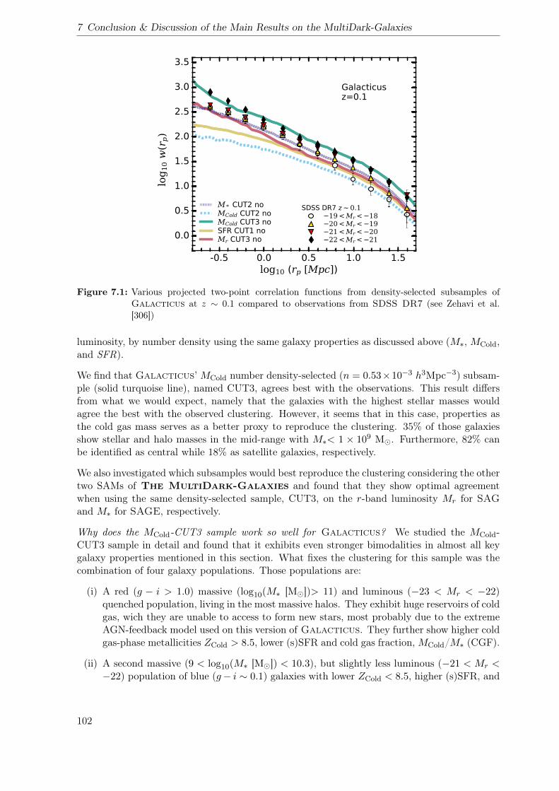
7 Conclusion & Discussion of the Main Results on the MultiDark-Galaxies

log10 (rp [Mpc])

log 1

0 w(r

p)

Galacticusz=0.1

SDSS DR7 z 0.1

-0.5 0.0 0.5 1.0 1.5

0.0

0.5

1.0

1.5

2.0

2.5

3.0

3.5

M * CUT2 noMCold CUT2 noMCold CUT3 noSFR CUT1 noMr CUT3 no

19 < Mr < 1820 < Mr < 1921 < Mr < 2022 < Mr < 21

Figure 7.1: Various projected two-point correlation functions from density-selected subsamples ofGalacticus at z ∼ 0.1 compared to observations from SDSS DR7 (see Zehavi et al.[306])

luminosity, by number density using the same galaxy properties as discussed above (M∗, MCold,and SFR).

We find that Galacticus’MCold number density-selected (n = 0.53×10−3 h3Mpc−3) subsam-ple (solid turquoise line), named CUT3, agrees best with the observations. This result differsfrom what we would expect, namely that the galaxies with the highest stellar masses wouldagree the best with the observed clustering. However, it seems that in this case, properties asthe cold gas mass serves as a better proxy to reproduce the clustering. 35% of those galaxiesshow stellar and halo masses in the mid-range with M∗< 1 × 109 M. Furthermore, 82% canbe identified as central while 18% as satellite galaxies, respectively.

We also investigated which subsamples would best reproduce the clustering considering the othertwo SAMs of The MultiDark-Galaxies and found that they show optimal agreementwhen using the same density-selected sample, CUT3, on the r-band luminosity Mr for SAGand M∗ for SAGE, respectively.

Why does the MCold-CUT3 sample work so well for Galacticus? We studied the MCold-CUT3 sample in detail and found that it exhibits even stronger bimodalities in almost all keygalaxy properties mentioned in this section. What fixes the clustering for this sample was thecombination of four galaxy populations. Those populations are:

(i) A red (g − i > 1.0) massive (log10(M∗ [M])> 11) and luminous (−23 < Mr < −22)quenched population, living in the most massive halos. They exhibit huge reservoirs of coldgas, wich they are unable to access to form new stars, most probably due to the extremeAGN-feedback model used on this version of Galacticus. They further show higher coldgas-phase metallicities ZCold > 8.5, lower (s)SFR and cold gas fraction,MCold/M∗ (CGF).

(ii) A second massive (9 < log10(M∗ [M]) < 10.3), but slightly less luminous (−21 < Mr <−22) population of blue (g− i ∼ 0.1) galaxies with lower ZCold < 8.5, higher (s)SFR, and

102

higher CGF .

(iii) A third lower massive population, living in smaller halos and also have smaller M∗, buttheir gas-phase metallicity is with ZCold > 8.5 as high as in (i).

(iv) A fourth population containing almost 50% of all galaxies of the total sample including:low massive, starforming, and blue galaxies; living in medium massive halos and hosting acentral galaxy. It is very likely that they fix the clustering at the smallest scales togetherwith the satellites. They further show very strong star formation, high CGFs, and lowZCold.

Are those bimodalities model dependent issues? It is not clear if Galacticus exhibits suchprominent bimodalities due to its modelling or calibration. As me mentioned before, the AGN-feedback, implemented in this version of Galacticus, is quite strong. We know further that,if the AGN feedback is recalibrated, different results regarding the stellar mass function orluminosities especially at higher redshift will be obtained. That is not surprising since theAGN feedback heavily controls the star formation. However, we chose Galacticus as ourpreferred model to study CMASS galaxies, because it provides stellar masses and luminosities ingood agreement with observations. This might not be the case if only the AGN feedback isrecalibrated. Furthermore, as we pointed out before, Galacticus was not recalibrated to theMDPL2 simulation either, but its most favourable recipe of parameters used. Therefore, it isremarkable that the model’s results are in such good agreement with observations. A detailedanalysis of Galacticus and its modelling and recalibration would be beyond of the scope ofthis thesis and we leave this work to further studies. We note that, the calibration of SAMs isa complicated topic, therefore we refer the reader to studies on the comparison of SAMs, as wementioned above, as well as to the works of Knebe et al. [150, 151] where effects of recalibrationin SAMs are studied.

Bimodalities as an opportunity to trace different populations ofgalaxies?

One of the key objective of this thesis is to shed light into the complex processes shaping galaxyproperties and driving galaxy formation and evolution over cosmic time. We have shown how tosystematically analyse the correlation of galaxy properties by means of their spatial distribution.It is known that galaxies and their clustering properties not only carry extensive information onthe underlying matter density field, but variations in the clustering performance also give clueson the intrinsic properties of a sample of galaxies regarding their formation and evolution (e.g.an assembly bias signal).

As shown by Montero-Dorta et al. [198] in their study of the galaxy assembly bias in BOSS-CMASSgalaxies, bimodalities are optimal tracers for intrinsic properties, which are suppose to shapea certain population of galaxies. In the case of the authors, they detected two population ofluminous red galaxies, where one is fast and the other slowly assembling their masses with time.We have seen for example in Fig. 10 in Paper I or in Fig. 10 in Paper II that Galacticusshows strong bimodalities in galaxy properties related to luminosity and metallicity. We furtherhave discussed in Chapter 4, that modelled LRGs from Galacticus show correlations of starformation related properties with halo mass and environment, which could be studied in futureworks. What remains unclear is, if and to what degree, this dependency emerges from theassembly of the dark matter halos, or from the model itself and its calibration. A more complexanalysis regarding the synergy of halo and galaxy properties is work in progress. We leave a

103

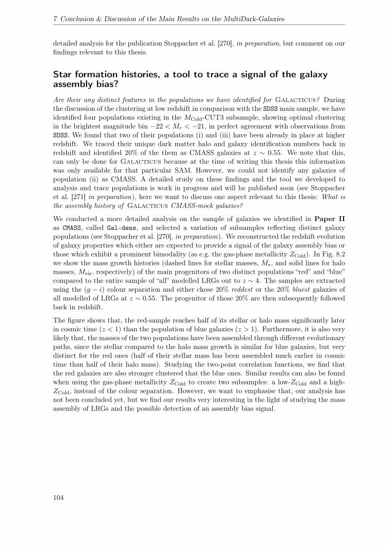
7 Conclusion & Discussion of the Main Results on the MultiDark-Galaxies

detailed analysis for the publication Stoppacher et al. [270], in preparation, but comment on ourfindings relevant to this thesis.

Star formation histories, a tool to trace a signal of the galaxyassembly bias?

Are their any distinct features in the populations we have identified for Galacticus? Duringthe discussion of the clustering at low redshift in comparison with the SDSSmain sample, we haveidentified four populations existing in the MCold-CUT3 subsample, showing optimal clusteringin the brightest magnitude bin −22 < Mr < −21, in perfect agreement with observations fromSDSS. We found that two of their populations (i) and (iii) have been already in place at higherredshift. We traced their unique dark matter halo and galaxy identification numbers back inredshift and identified 20% of the them as CMASS galaxies at z ∼ 0.55. We note that this,can only be done for Galacticus because at the time of writing this thesis this informationwas only available for that particular SAM. However, we could not identify any galaxies ofpopulation (ii) as CMASS. A detailed study on these findings and the tool we developed toanalysis and trace populations is work in progress and will be published soon (see Stoppacheret al. [271] in preparation), here we want to discuss one aspect relevant to this thesis: What isthe assembly history of Galacticus CMASS-mock galaxies?

We conducted a more detailed analysis on the sample of galaxies we identified in Paper IIas CMASS, called Gal-dens, and selected a variation of subsamples reflecting distinct galaxypopulations (see Stoppacher et al. [270], in preparation). We reconstructed the redshift evolutionof galaxy properties which either are expected to provide a signal of the galaxy assembly bias orthose which exhibit a prominent bimodality (as e.g. the gas-phase metallicity ZCold). In Fig. 8.2we show the mass growth histories (dashed lines for stellar masses, M∗, and solid lines for halomasses, Mvir, respectively) of the main progenitors of two distinct populations “red” and “blue”compared to the entire sample of “all” modelled LRGs out to z ∼ 4. The samples are extractedusing the (g − i) colour separation and either chose 20% reddest or the 20% bluest galaxies ofall modelled of LRGs at z ∼ 0.55. The progenitor of those 20% are then subsequently followedback in redshift.

The figure shows that, the red-sample reaches half of its stellar or halo mass significantly laterin cosmic time (z < 1) than the population of blue galaxies (z > 1). Furthermore, it is also verylikely that, the masses of the two populations have been assembled through different evolutionarypaths, since the stellar compared to the halo mass growth is similar for blue galaxies, but verydistinct for the red ones (half of their stellar mass has been assembled much earlier in cosmictime than half of their halo mass). Studying the two-point correlation functions, we find thatthe red galaxies are also stronger clustered that the blue ones. Similar results can also be foundwhen using the gas-phase metallicity ZCold to create two subsamples: a low-ZCold and a high-ZCold, instead of the colour separation. However, we want to emphasise that, our analysis hasnot been concluded yet, but we find our results very interesting in the light of studying the massassembly of LRGs and the possible detection of an assembly bias signal.

104

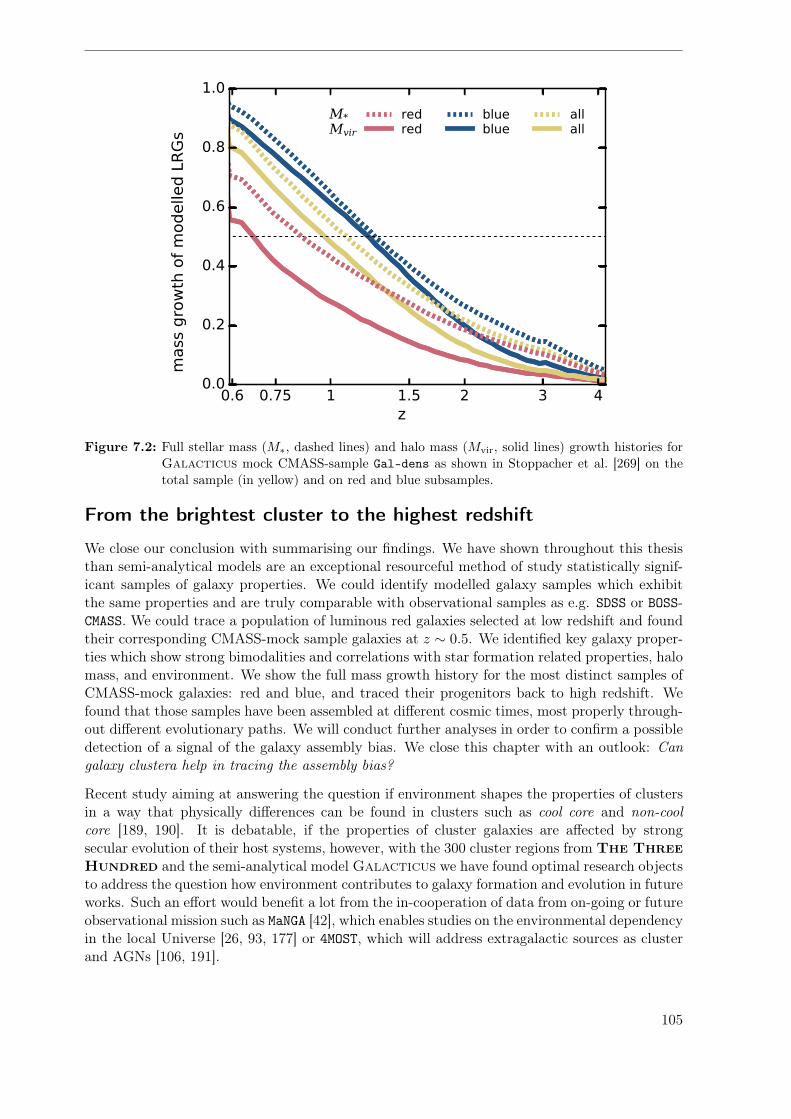
z

mas

s gro

wth

of m

odel

led

LRGs

M*Mvir

redred

blueblue

allall

0.6 0.75 1 1.5 2 3 40.0

0.2

0.4

0.6

0.8

1.0

Figure 7.2: Full stellar mass (M∗, dashed lines) and halo mass (Mvir, solid lines) growth histories forGalacticus mock CMASS-sample Gal-dens as shown in Stoppacher et al. [269] on thetotal sample (in yellow) and on red and blue subsamples.

From the brightest cluster to the highest redshift

We close our conclusion with summarising our findings. We have shown throughout this thesisthan semi-analytical models are an exceptional resourceful method of study statistically signif-icant samples of galaxy properties. We could identify modelled galaxy samples which exhibitthe same properties and are truly comparable with observational samples as e.g. SDSS or BOSS-CMASS. We could trace a population of luminous red galaxies selected at low redshift and foundtheir corresponding CMASS-mock sample galaxies at z ∼ 0.5. We identified key galaxy proper-ties which show strong bimodalities and correlations with star formation related properties, halomass, and environment. We show the full mass growth history for the most distinct samples ofCMASS-mock galaxies: red and blue, and traced their progenitors back to high redshift. Wefound that those samples have been assembled at different cosmic times, most properly through-out different evolutionary paths. We will conduct further analyses in order to confirm a possibledetection of a signal of the galaxy assembly bias. We close this chapter with an outlook: Cangalaxy clustera help in tracing the assembly bias?

Recent study aiming at answering the question if environment shapes the properties of clustersin a way that physically differences can be found in clusters such as cool core and non-coolcore [189, 190]. It is debatable, if the properties of cluster galaxies are affected by strongsecular evolution of their host systems, however, with the 300 cluster regions from The ThreeHundred and the semi-analytical model Galacticus we have found optimal research objectsto address the question how environment contributes to galaxy formation and evolution in futureworks. Such an effort would benefit a lot from the in-cooperation of data from on-going or futureobservational mission such as MaNGA [42], which enables studies on the environmental dependencyin the local Universe [26, 93, 177] or 4MOST, which will address extragalactic sources as clusterand AGNs [106, 191].

105

7 Conclusion & Discussion of the Main Results on the MultiDark-Galaxies

In summary, within this thesis work we presented interesting correlations of populations ofluminous red galaxies with their large-scale environment and draw conclusions on their formationand evolution using a semi-analytical model. We concluded this thesis with an outlook on furtherworks and emphasis the conduction of full-encompassing studies exploring all possible parameterspaces on small and large-scales, incooperating isolated and dens environments, as well as takingadvantage of all available astrophysical and computational resources; from the brightest clusterto the highest redshift ... to be continued.

106

8 Conclusión & Discusión de losResultados Generales de lasThe MultiDark-Galaxies

En esta disertación adoptamos las The MultiDark-Galaxies, cuyo desarrollo y publi-cación formaron parte de este trabajo de tesis, como nuestros principales objetos de investi-gación. Consisten en tres catálogos que contienen amplios conjuntos de propiedades de galax-ias generadas al completar la simulación cosmológica de N -cuerpos MultiDark Planck 2(MDPL2) con galaxias utilizando tres modelos semi-analíticos (SAM) diferentes. Dedicamos elChapter 3 a llevar a cabo un extenso análisis e interpretación de los resultados y al estudiode la agrupación de galaxias masivas en z = 0.1 en comparación con las galaxias de la muestraprincipal de SDSS Hemos mostrado cómo seleccionar galaxias rojas luminosas imitando la selec-ción fotométrica de BOSS-CMASS con nuestro SAM preferente, Galacticus, en el Chapter 4.De este modo, encontramos una dependencia de las propiedades relacionadas con la formaciónestelar y la metalicidad respecto al entorno. En el Chapter 5 hemos comparado regiones decúmulos simulados de The Three Hundred clusters usando modelos diferentes estrate-gias de modelización ejecutadas en la misma simulación de materia oscura que Galacticus,obteniendo que nuestro modelo reproduce propiedades de cúmulos básicas como ninguno de losmodelos utilizados en este estudio. En este capítulo, discutimos los principales resultados denuestros estudios sobre The MultiDark-Galaxies, resumidos en el Chapter 6. Poste-riormente proporcionamos nuestra conclusión global y una perspectiva para futuros proyectossobre el sesgo de ensamblaje de galaxias.

¿Un modelo para medirlos a todos?

Se ha demostrado que las predicciones de los SAM son muy útiles para la comunidad cuandose trata de la llamada física de “sub-cuadrícula”, es decir, la parte de la física que actualmentese comprende mal o está más allá de los límites de resolución. Estos modelos están lejos de serperfectos, pero gracias a intentos como The SAM Comparison Project, ver Knebe et al.[149, 150] se ha recorrido un largo camino. En este y otros proyectos similares, se ha realizadoun esfuerzo colectivo para poner a prueba los modelos de formación de galaxias comparando suspredicciones cuando se usan las mismas simulaciones o calibraciones de N -cuerpos. Se esperabaque los SAM produjeran resultados comparables, sin embargo, los resultados no coincidían tanbien como se esperaba.

Es desconcertante que las predicciones de los SAM u otros modelos de formación de galaxias seantan diversas, hasta el punto de mostrar diferencias de órdenes de magnitud entre los modelos[see e.g. 151, 229]. Además, la mayoría de los códigos SAM concuerdan adecuadamente conlas propiedades observacionales en z ∼ 0 (donde además se han calibrados), pero reproducende forma pobre las luminosidades y los colores a alto redshift, como se ha demostrado en estatesis en el caso de Galacticus (ver Chapter 4 y Chapter 3). Una forma de abordar estasituación consiste en buscar mejoras adicionales y calibraciones más precisas de los SAM. Sinembargo, a menudo las propiedades observacionales involucradas en el proceso de calibración delos modelos muestran también variaciones significativas y no se pueden usar para restriccionesrealmente precisas, especialmente cuando consideramos valores más altos del redshift (ver, por

107

8 Conclusión & Discusión de los Resultados Generales de las The MultiDark-Galaxies

ejemplo, la densidad cósmica de la tasa de formación estelar de Madau and Dickinson [183] ensu Fig. 9).

La relevancia de la comparación y validación de los distintos SAM en esta tesis se basa en laampliación de nuestro conocimiento sobre problemas comunes de modelado y calibración quepuedan afectar a los resultados. A la larga, esto garantiza una mejor comprensión y evaluaciónde los resultados obtenidos por los SAM. Proyectos como The MultiDark-Galaxies yThe Three Hundred se han beneficiado de ese conocimiento y la conclusión extraída dela comparación de los SAM se ha incorporado posteriormente a esta tesis. Nuestra principalrecomendación de cara a clarificar la compleja interacción de las propiedades galácticas en elmodelado semi-analítico sería el seguimiento automático de las propiedades clave en cada pasode tiempo de la simulación. Siempre que esas propiedades clave, que podrían estar acompañadaspor, por ejemplo, análisis estadísticos bayesianos, se obtengan de la misma manera para cadaSAM, se podrían obtener pistas sobre en qué etapa los resultados de los diferentes modeloscomienzan a divergir. Por lo tanto, sugerimos que el desarrollo de los SAM, así como susestrategias y calibraciones, sea lo más transparente posible.

Otra posible respuesta sería considerar que muchos SAM pueden producir ciertos resultadosclave en un grado razonable, sin considerar que un solo modelo en particular pueda reproducirloscon precisión. Esto garantizaría una determinada evaluación de calidad y podría permitirnosalcanzar una mejor comprensión de los SAM y su sistemática.

La compleja interacción de las propiedades de la galaxia desafíala interpretación de la agrupación de galaxias

En el Chapter 3 presentamos resultados de las funciones de correlación de dos puntos (2pCF)de submuestras de las The MultiDark-Galaxies. La selección de galaxias considerandopropiedades distintas como la masa estelar (M∗) básicamente implica la restricción del análisisa galaxias más masivas, en lugar de a galaxias con grandes reservas de gas frío (MCold), es decir,galaxias con menor masa estelar. En cambio, si usamos la tasa de formación de estrellas (SFR),se da una selección preferente de galaxias con formación estelar activa. Elegir un conjunto degalaxias u otro no implica sesgar implícitamente los resultados, sino que se trata más bien de unaherramienta útil para analizar la implementación de diferentes modelos y descubrir el compor-tamiento de agrupamiento en diferentes regímenes de masa, gas frío o SFR. Las característicasde la muestra seleccionada, es decir, si por ejemplo se trata de galaxias masivas o activas, sereflejarán en la agrupación, ya que por ejemplo sabemos que las galaxias rojas masivas estánmás agrupadas que las galaxias azules menos masivas [273].

El hecho de que el rendimiento de agrupación de cierto número de muestras seleccionadas pordensidad concuerde mejor entre sí, debe ser comprendido, para poder concluir si la diferencia enla agrupación surge de una causa física (por ejemplo, depende del entorno o de las interaccionesde galaxias) o ha sido introducido por efectos de selección. Por ejemplo, los 2pCF de las muestrasseleccionadas por masa estelar muestran en general una menor variación en la agrupación entremodelos. Sin embargo, si verificamos los umbrales aplicados a las masas estelares o las tasas deformación estelar, respectivamente, la variación en la masa estelar es cuatro veces mayor quela obtenida en la SFR. Esto deja espacio para diversas interpretaciones. Por un lado, la masaestelar parece ser una de las propiedades galácticas más estables para seleccionar submuestras,pero por otro lado, las funciones de SFR calculadas para los tres SAMs coinciden mucho mejorcon las observaciones que las funciones de masa estelar (ver Fig. 1 y Fig. 2 en Paper I).

108

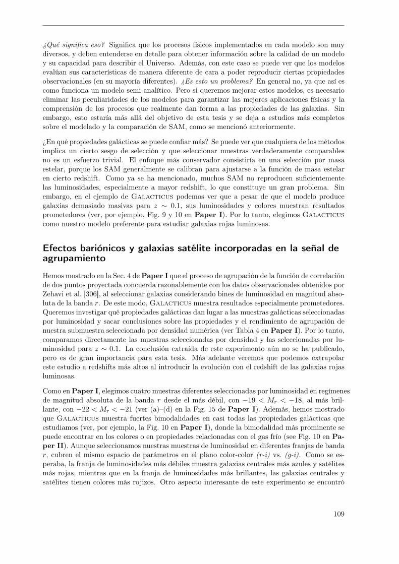
¿Qué significa eso? Significa que los procesos físicos implementados en cada modelo son muydiversos, y deben entenderse en detalle para obtener información sobre la calidad de un modeloy su capacidad para describir el Universo. Además, con este caso se puede ver que los modelosevalúan sus características de manera diferente de cara a poder reproducir ciertas propiedadesobservacionales (en su mayoría diferentes). ¿Es esto un problema? En general no, ya que así escomo funciona un modelo semi-analítico. Pero si queremos mejorar estos modelos, es necesarioeliminar las peculiaridades de los modelos para garantizar las mejores aplicaciones físicas y lacomprensión de los procesos que realmente dan forma a las propiedades de las galaxias. Sinembargo, esto estaría más allá del objetivo de esta tesis y se deja a estudios más completossobre el modelado y la comparación de SAM, como se mencionó anteriormente.

¿En qué propiedades galácticas se puede confiar más? Se puede ver que cualquiera de los métodosimplica un cierto sesgo de selección y que seleccionar muestras verdaderamente comparablesno es un esfuerzo trivial. El enfoque más conservador consistiría en una selección por masaestelar, porque los SAM generalmente se calibran para ajustarse a la función de masa estelaren cierto redshift. Como ya se ha mencionado, muchos SAM no reproducen suficientementelas luminosidades, especialmente a mayor redshift, lo que constituye un gran problema. Sinembargo, en el ejemplo de Galacticus podemos ver que a pesar de que el modelo producegalaxias demasiado masivas para z ∼ 0.1, sus luminosidades y colores muestran resultadosprometedores (ver, por ejemplo, Fig. 9 y 10 en Paper I). Por lo tanto, elegimos Galacticuscomo nuestro modelo preferente para estudiar galaxias rojas luminosas.

Efectos bariónicos y galaxias satélite incorporadas en la señal deagrupamiento

Hemos mostrado en la Sec. 4 dePaper I que el proceso de agrupación de la función de correlaciónde dos puntos proyectada concuerda razonablemente con los datos observacionales obtenidos porZehavi et al. [306], al seleccionar galaxias considerando bines de luminosidad en magnitud abso-luta de la banda r. De este modo, Galacticus muestra resultados especialmente prometedores.Queremos investigar qué propiedades galácticas dan lugar a las muestras galácticas seleccionadaspor luminosidad y sacar conclusiones sobre las propiedades y el rendimiento de agrupación denuestra submuestra seleccionada por densidad numérica (ver Tabla 4 en Paper I). Por lo tanto,comparamos directamente las muestras seleccionadas por densidad y las seleccionadas por lu-minosidad para z ∼ 0.1. La conclusión extraída de este experimento aún no se ha publicado,pero es de gran importancia para esta tesis. Más adelante veremos que podemos extrapolareste estudio a redshifts más altos al introducir la evolución con el redshift de las galaxias rojasluminosas.

Como enPaper I, elegimos cuatro muestras diferentes seleccionadas por luminosidad en regímenesde magnitud absoluta de la banda r desde el más débil, con −19 < Mr < −18, al más bril-lante, con −22 < Mr < −21 (ver (a)–(d) en la Fig. 15 de Paper I). Además, hemos mostradoque Galacticus muestra fuertes bimodalidades en casi todas las propiedades galácticas queestudiamos (ver, por ejemplo, la Fig. 10 en Paper I), donde la bimodalidad más prominente sepuede encontrar en los colores o en propiedades relacionadas con el gas frío (see Fig. 10 en Pa-per II). Aunque seleccionamos nuestras muestras de luminosidad en diferentes franjas de bandar, cubren el mismo espacio de parámetros en el plano color-color (r-i) vs. (g-i). Como se es-peraba, la franja de luminosidades más débiles muestra galaxias centrales más azules y satélitesmás rojas, mientras que en la franja de luminosidades más brillantes, las galaxias centrales ysatélites tienen colores más rojizos. Otro aspecto interesante de este experimento se encontró

109

8 Conclusión & Discusión de los Resultados Generales de las The MultiDark-Galaxies

log10 (rp [Mpc])

log 1

0 w(r

p)

Galacticusz=0.1

SDSS DR7 z 0.1

-0.5 0.0 0.5 1.0 1.5

0.0

0.5

1.0

1.5

2.0

2.5

3.0

3.5

M * CUT2 noMCold CUT2 noMCold CUT3 noSFR CUT1 noMr CUT3 no

19 < Mr < 1820 < Mr < 1921 < Mr < 2022 < Mr < 21

Figure 8.1: Varias funciones de correlación de dos puntos proyectadas de submuestras seleccionadaspor densidad de Galacticus para z ∼ 0.1, comparadas con observaciones de la SDSSDR7 (ver Zehavi et al. [306])

en las galaxias centrales, ya que todas las submuestras exhiben una tasa de formación estelarespecífica similar, con valores de −9 < log10(sSFR [yr−1]) < −10, independientemente de susmasas estelares o de las masas de sus halos. Además, la franja de luminosidades más brillantescomprende todas las masas estelares y de halos, mientras que la franja de luminosidades débilessolo comprende los valores más bajos de ambas propiedades.

Destacamos que la única propiedad que muestra una distribución diversa entre las masas de haloy estelares es la masa de gas frío MCold. La masa de gas frío más baja se puede encontrar enlos halos de materia oscura más masivos, con valores de log10(MHalo [M]) > 12, y en la franjade luminosidades medias, con valores de −20 < Mr < −19 y −21 < Mr < −20, mientras quela mayor cantidad de gas frío se encuentra en halos poco masivos, con log10(MHalo [M]) ∼ 11.Esto no es sorprendente, ya que estudios observacionales recientes han confirmado la tendenciade que las galaxias rojas luminosas tienen poca cantidad de gas frío [23].

¿Qué muestras reproducen mejor la agrupación de galaxias brillantes en z ∼ 0.1? En la Fig.1.1 mostramos mediciones de los 2pCF tal como se muestra en la Fig. 15 de Paper I, encomparación con la agrupación observacional de las galaxias de SDSS para z ∼ 0.1 Zehaviet al. [306], pero esta vez no seleccionamos submuestras usando franjas de luminosidad, sinopor criterios de densidad numérica, usando las mismas propiedades galácticas ya comentadasanteriormente (M∗, MCold y SFR).

Hallamos que la submuestra de MCold de Galacticus seleccionada por densidad numérica(n = 0.53 × 10−3 h3Mpc−3) (línea turquesa continua), llamada CUT3, coincide mejor con lasobservaciones. Este resultado difiere de lo que esperaríamos, a saber, que las galaxias con lasmasas estelares más altas coincidirían con la agrupación observada. Sin embargo, parece que eneste caso las propiedades como la masa de gas frío sirven mejor como proxy para reproducir elagrupamiento. El 35% de esas galaxias muestran masas estelares y de halo en el rango medioconM∗ < 1×109 M, y el 82% se puede identificar como central y el 18% como galaxias satélite,

110

respectivamente.

También hemos investigado qué submuestras reproducirían mejor la agrupación de los otros dosSAM del proyectoThe MultiDark-Galaxies y encontramos que muestran una concordan-cia óptima cuando se usa la misma muestra seleccionada por densidad, CUT3, en la luminosidadde la banda r, Mr, para SAG y en la masa estelar M∗ para SAGE, respectivamente.

¿Por qué la muestraMCold-CUT3 funciona tan bien para Galacticus? Estudiamos la muestraMCold-CUT3 en detalle y descubrimos que exhibe bimodalidades aún más fuertes en casi todaslas propiedades galácticas clave mencionadas en esta sección. Lo que produjo el buen resultadodel agrupamiento para esta muestra fue la combinación de cuatro poblaciones de galaxias:

(i) Una población roja (g− i > 1.0) masiva (log10(M∗ [M]) > 11) y luminosa (−23 < Mr <−22) quenched que vive en los halos más masivos. Tienen enormes reservas de gas frío,no pueden formar nuevas estrellas, probablemente debido al modelo de retroalimentaciónde AGN extrema utilizado en esta versión de Galacticus. Además muestran una mayormetalicidad de la fase gaseosa fría, ZCold > 8.5, y menores (s)SFR y fracción de gas frío,MCold/M∗ (CGF).

(ii) Una segunda población masiva (9 < log10(M∗ [M]) < 10.3) pero ligeramente menosluminosa (−21 < Mr < −22) de galaxias azules (g− i ∼ 0.1), con menor ZCold (menor de8.5), mayor (s)SFR y CGFs.

(iii) Una tercera población menos masiva, que vive en halos más pequeños, con M∗ pequeña,pero con la metalicidad de la fase gaseosa fría ZCold > 8.5 tan alta como en (i).

(iv) Una cuarta población que contiene casi el 50% de todas las galaxias de la muestra total,incluyendo galaxias de baja masa, de formación estelar y azules que viven en halos de masamedia, que albergan una galaxia central. Es muy probable que configuren la agrupaciónen las escalas más pequeñas, junto con los satélites. Además, muestran una formaciónestelar muy fuerte, CGFs altos y ZCold bajo.

¿Son esas bimodalidades cuestiones dependientes del modelo? No está claro si Galacticusexhibe bimodalidades tan prominentes debido a su modelado o calibración. Como hemos men-cionado antes, la AGN feedback, implementada en esta versión de Galacticus, es bastantefuerte. Sabemos además que si la AGN feedback se recalibra, se obtienen resultados diferentescon respecto a la función de masa estelar o las luminosidades, especialmente a valores altos delredshift. Eso no es sorprendente, ya que la feedback de AGN controla en gran medida la forma-ción estelar. Sin embargo, elegimos Galacticus como nuestro modelo preferido para estudiarlas galaxias CMASS porque proporcionaba masas estelares y luminosidades concordantes conlos datos observacionales. Este podría no ser el caso si solo se recalibra la feedback de AGN.Además, como señalamos antes, Galacticus tampoco se recalibró con la simulación MDPL2,sino que se utilizó su configuración de parámetros más favorable. Por lo tanto, es notable quelos resultados del modelo estén tan de acuerdo con las observaciones. Un análisis detallado deGalacticus y su modelado y recalibración estaría más allá del alcance de esta tesis, y dejamoseste trabajo para futuros estudios. La calibración de los SAMs es un tema complicado, por lotanto, remitimos al lector a estudios sobre la comparación de SAMs, como mencionamos ante-riormente, así como a los trabajos Knebe et al. [150, 151], donde se estudian los efectos de larecalibración en los SAM.

111

8 Conclusión & Discusión de los Resultados Generales de las The MultiDark-Galaxies

¿Las bimodalidades como una oportunidad para rastreardiferentes poblaciones de galaxias?

Uno de los objetivos clave de esta tesis fue arrojar luz sobre los complejos procesos que configu-ran las propiedades de las galaxias y que impulsan la formación y evolución de las galaxias a lolargo de la edad de universo. Hemos mostrado cómo analizar sistemáticamente la correlación delas propiedades de las galaxias por medio de su distribución espacial, ya que las galaxias y suspropiedades de agrupamiento no solo contienen información extensiva sobre el campo de densi-dad de materia subyacente, per también las variaciones en las propiedades de agrupamiento daclues de las properidades instrinsicas de una muestra de galaxias en el contexto de su formacióny evolución (pro ejemplo un se´ nal del sesgo de ensamblaje de la masa).

Como se muestra Montero-Dorta et al. [198] en su estudio del sesgo de ensamblaje de la masade las galaxias en las galaxias BOSS-CMASS, las bimodalidades son trazadores óptimos para laspropiedades intrínsecas que configuran una determinada población de galaxias. En el casode los autores, detectaron dos poblaciones de galaxias rojas luminosas, donde una ensamblarápidamente sus masas con el tiempo y la otra lo hace más lentamente. Hemos visto, porejemplo, en la Fig. 10 en Paper I o en la Fig. 10 en Paper II que Galacticus muestra fuertesbimodalidades en las propiedades de la galaxia relacionadas con la luminosidad y la metalicidad.Más adelante hemos discutido en el Chapter 4, que los LRG modelados de Galacticusmuestran correlaciones de las propiedades relacionadas con la formación de estrellas con lamasa de halo y el entorno, lo que sentará las bases para futuros estudios sobre el tema. Loque no está claro es, si y en qué medida, esta dependencia surge del ensamblaje de los halosde materia oscura o del modelo en sí y su calibración. Se está trabajando en un análisis máscomplejo con respecto a la sinergia de las propiedades de halo y galaxia. Dejamos un análisisdetallado para la publicación, Stoppacher et al. [270], pero comentamos nuestros resultados másrelevantes en esta tesis.

¿Las historias de formación estelar son una herramienta pararastrear una señal del sesgo de ensamblaje de galaxias?

¿Hay alguna característica distintiva en las poblaciones que hemos identificado en Galacticus?Durante la discusión de la agrupación a bajo desplazamiento al rojo en comparación con lamuestra principal de SDSS, hemos identificado cuatro poblaciones existentes en la submuestraMCold-CUT3, mostrando una agrupación óptima en el bin de magnitud más brillante −22 <Mr < −21, en perfecto acuerdo con observaciones de SDSS. Hemos encontrado que dos desus poblaciones (i) y (iii) ya han estado en su lugar en los desplazamientos al rojo más altos.Rastreamos sus números únicos de identificación para el halo de materia oscura y para la galaxiaa lo largo del desplazamiento al rojo, e identificamos el 20% de las galaxias como CMASS enz ∼ 0.55. Notamos que esto solo se puede hacer para Galacticus porque en el momento deescribir esta tesis esa información solo estaba disponible para este SAM.in embargo, no pudimosidentificar ninguna galaxia de población (ii) como CMASS . Un estudio detallado sobre estosresultados y la herramienta que desarrollamos para analizar y rastrear poblaciones está enprogreso y se publicará pronto (ver Stoppacher et al. [271]), aquí queremos discutir un aspectorelevante para esta tesis: ¿Cuál es la historia de ensamblaje de galaxias simuladas de la muestrade CMASS de Galacticus?

Realizamos un análisis más detallado de la muestra de galaxias que identificamos en Paper IIcomo CMASS, llamado Gal-dens, y seleccionamos unas variaciónes de submuestras que reflejan

112

z

creci

mie

nto

de m

asa

s d

e L

RG

s m

od

ela

das

M*Mvir

rojorojo

azulazul

todostodos

0.6 0.75 1 1.5 2 3 40.0

0.2

0.4

0.6

0.8

1.0

Figure 8.2: Historias de crecimiento de la masa estelar (M∗, líneas discontinuas) y de la masa de halo(MHalo, líneas continuas) de galaxias simuladas de la muestra de CMASS de Galacticus,Gal-dens como se muestra en Stoppacher et al. [269], para la muestra total (en amarillo)y para las submuestras roja y azul.

distintas poblaciones de galaxias (ver Stoppacher et al. [270]). Reconstruimos la evolución de laspropiedades de la galaxia con el desplazamiento al rojo, que se espera que proporcionen una señaldel sesgo de ensamblaje de galaxias en aquellas que exhiben una bimodalidad prominente (como,por ejemplo, la metalicidad en fase gaseosa ZCold). En la Fig. 8.2 mostramos las historias decrecimiento en masa (líneas discontinuas para masas estelares,M∗ y líneas continuas para masasde halo, MHalo, respectivamente) de los principales progenitores de dos poblaciones distintas“rojo” y “azul” en comparación con la totalidad muestra de “todos” los LRG modelados a z ∼ 4.Las muestras se extraen usando la separación de color (g-i) y se seleciona el 20% de galaxias másrojas o el 20% de galaxias más azules de todos los LRG modelados en z ∼ 0.55. El progenitorde ese 20% es seguido posteriormente a lo largo del desplazamiento al rojo.

La figura muestra que la muestra roja alcanza la mitad de su masa estelar o del halo significa-tivamente más tarde en tiempo cósmico (z < 1) que la población de galaxias azules (z > 1).Además, también es muy probable que las masas de las dos poblaciones se hayan ensambladoa través de diferentes caminos evolutivos, ya que el crecimiento de masa estelar en compara-ción con la del halo es similar para las galaxias azules, pero es muy distinto para las rojas (lamitad de su masa estelar ha sido ensamblada mucho antes en el tiempo cósmico que la mitadde su masa del halo). Al estudiar las funciones de correlación de dos puntos, encontramos quelas galaxias rojas también están más fuertemente agrupadas que las azules.También se puedenencontrar resultados similares cuando se usa la metalicidad en fase gaseosa ZCold para crear dossubmuestras: un ZCold bajo y un ZCold alto, en lugar de la separación de color. Sin embargo,queremos enfatizar que nuestro análisis aún no se ha concluido, pero que nuestros resultados sonmuy interesantes a la luz del estudio del ensamblaje en masa de los LRGs y la posible detecciónde una señal de sesgo de ensamblaje de galaxias.

113

8 Conclusión & Discusión de los Resultados Generales de las The MultiDark-Galaxies

Desde el grupo más brillante hasta el desplazamiento al rojo másalto

Cerramos nuestra conclusión con un resumen de nuestros resultados. Hemos demostrado alo largo de esta tesis que los modelos semi-analíticos son un método excepcionalmente inge-nioso para estudiar las propiedades de las galaxias en muestras estadísticamente significativas.Podemos identificar muestras de galaxias modeladas que exhiben las mismas propiedades y sonrealmente comparables con muestras de observación como, por ejemplo SDSS o BOSS-CMASS.Podemos rastrear una población de galaxias rojas luminosas selecionado a bajo desplazamientoal rojo, para encontrar sus galaxias de muestra simuladas CMASS correspondientes a z ∼ 0.5.Identificamos propiedades clave de galaxias que muestran fuertes bimodalidades y correlacionescon las propiedades relacionadas con la formación de estrellas, la masa de halo y el entorno.Mostramos el historial completo de crecimiento de la masa para las muestras más distintas de lasgalaxias de CMASS muestra simulada: roja y azul, y rastreamos sus progenitores hasta un altodesplazamiento al rojo. Descubrimos que esas muestras se han ensamblado en diferentes tiem-pos cósmicos, o más adecuadamente a lo largo de diferentes caminos evolutivos. Realizaremosanálisis adicionales para confirmar una posible detección de una señal del sesgo de ensamblajede galaxias. Cerramos este capítulo con una prvision: ¿Pueden los cúmulos de galaxias ayudara rastrear el sesgo de ensamblaje?

Estudio reciente con el objetivo de responder a la pregunta de si el entorno da forma a laspropiedades del cúmulo de galaxias de manera que se puedan encontrar diferencias físicas, comoun cúmulo cool core o non-cool core [189, 190]. Se puede debatir, si las propiedades de los cú-mulos de galaxias se ven afectadas por una fuerte evolución secular de sus sistemas anfitriones,sin embargo, con las 300 regiones de cúmulos de galaxias de The Three Hundred y elmodelo semi-analítico Galacticus, hemos encontrado objetos de investigación óptimos paraabordar en el futuro esta cuestión, de cómo el entorno contribuye a la formación y evolución delas galaxias. Tal esfuerzo se beneficiaría mucho de la cooperación con los datos de misiones deobservación en curso o futuras, como MaNGA [42], que permite realizar estudios sobre la dependen-cia ambiental en el universo local [26, 93, 177] o 4MOST que abordará las fuentes extragalácticascomo cúmulos de galaxias y AGNs [106, 191].

En resumen, dentro de este trabajo de tesis presentamos correlaciones interesantes de pobla-ciones de galaxias rojas luminosas con su entorno a gran escala y sacamos conclusiones sobresu formación y evolución utilizando un modelo semi-analítico. Concluimos esta tesis con unbosquejo sobre trabajos futuros y sobre la realización de estudios completos que exploren todoslos parámetros posibles de escalas pequeña y gran escala, que incluyen los entornos aislados ydensos, y que se aprovechen de todos los recursos astrofísicos y computacionales disponibles;desde el cúmulo más brillante hasta el desplazamiento al rojo más alto ... continuará.

114

Bibliography[1] K. N. Abazajian, J. K. Adelman-McCarthy, M. A. Agüeros, S. S. Allam, C. Allende Prieto, D. An, K. S. J. Anderson,

S. F. Anderson, J. Annis, N. A. Bahcall, and et al. The Seventh Data Release of the Sloan Digital Sky Survey.ApJS, 182:543-558, June 2009. doi: 10.1088/0067-0049/182/2/543.

[2] D. Adams. The Salmon of Doubt: Hitchhiking the Galaxy One Last Time. Hitchhiker’s Guide to the Galaxy. RandomHouse Publishing Group, 2005. ISBN 9780345484499. URL https://books.google.es/books?id=DpIwyu_ZW9AC.

[3] I. Agullo and L. Parker. Non-Gaussianities and the stimulated creation of quanta in the inflationary universe.Phys. Rev. D, 83(6):063526, Mar 2011. doi: 10.1103/PhysRevD.83.063526.

[4] S. Alam, M. Ata, S. Bailey, F. Beutler, D. Bizyaev, J. A. Blazek, A. S. Bolton, J. R. Brownstein, A. Burden, C.-H.Chuang, J. Comparat, A. J. Cuesta, K. S. Dawson, D. J. Eisenstein, S. Escoffier, H. Gil-Marín, J. N. Grieb, N. Hand,S. Ho, K. Kinemuchi, D. Kirkby, F. Kitaura, E. Malanushenko, V. Malanushenko, C. Maraston, C. K. McBride,R. C. Nichol, M. D. Olmstead, D. Oravetz, N. Padmanabhan, N. Palanque-Delabrouille, K. Pan, M. Pellejero-Ibanez, W. J. Percival, P. Petitjean, F. Prada, A. M. Price-Whelan, B. A. Reid, S. A. Rodríguez-Torres, N. A. Roe,A. J. Ross, N. P. Ross, G. Rossi, J. A. Rubiño-Martín, S. Saito, S. Salazar-Albornoz, L. Samushia, A. G. Sánchez,S. Satpathy, D. J. Schlegel, D. P. Schneider, C. G. Scóccola, H.-J. Seo, E. S. Sheldon, A. Simmons, A. Slosar, M. A.Strauss, M. E. C. Swanson, D. Thomas, J. L. Tinker, R. Tojeiro, M. V. Magaña, J. A. Vazquez, L. Verde, D. A.Wake, Y. Wang, D. H. Weinberg, M. White, W. M. Wood-Vasey, C. Yèche, I. Zehavi, Z. Zhai, and G.-B. Zhao. Theclustering of galaxies in the completed SDSS-III Baryon Oscillation Spectroscopic Survey: cosmological analysis ofthe DR12 galaxy sample. MNRAS, 470(3):2617–2652, Sep 2017. doi: 10.1093/mnras/stx721.

[5] S. Alam, Y. Zu, J. A. Peacock, and R. Mand elbaum. Cosmic web dependence of galaxy clustering and quenchingin SDSS. MNRAS, 483(4):4501–4517, Mar 2019. doi: 10.1093/mnras/sty3477.

[6] C. Almeida, C. M. Baugh, D. A. Wake, C. G. Lacey, A. J. Benson, R. G. Bower, and K. Pimbblet. Luminous redgalaxies in hierarchical cosmologies. MNRAS, 386:2145–2160, June 2008. doi: 10.1111/j.1365-2966.2008.13179.x.

[7] S. Amarantidis, J. Afonso, H. Messias, B. Henriques, A. Griffin, C. Lacey, C. d. P. Lagos, V. Gonzalez-Perez,Y. Dubois, M. Volonteri, I. Matute, C. Pappalardo, Y. Qin, R.-R. Chary, and R. P. Norris. The first supermassiveblack holes: indications from models for future observations. MNRAS, 485(2):2694–2709, May 2019. doi: 10.1093/mnras/stz551.

[8] L. Amendola and S. Tsujikawa. Dark Energy. 2015.[9] T. J. Armitage, D. J. Barnes, S. T. Kay, Y. M. Bahé, C. Dalla Vecchia, R. A. Crain, and T. Theuns. The

Cluster-EAGLE project: velocity bias and the velocity dispersion-mass relation of cluster galaxies. MNRAS, 474(3):3746–3759, Mar 2018. doi: 10.1093/mnras/stx3020.

[10] M. C. Artale, I. Zehavi, S. Contreras, and P. Norberg. The impact of assembly bias on the halo occupation inhydrodynamical simulations. MNRAS, 480:3978–3992, Nov. 2018. doi: 10.1093/mnras/sty2110.

[11] I. K. Baldry, K. Glazebrook, J. Brinkmann, Ž. Ivezić, R. H. Lupton, R. C. Nichol, and A. S. Szalay. Quantifyingthe Bimodal Color-Magnitude Distribution of Galaxies. ApJ, 600(2):681–694, Jan 2004. doi: 10.1086/380092.

[12] I. K. Baldry, K. Glazebrook, and S. P. Driver. On the galaxy stellar mass function, the mass-metallicity relationand the implied baryonic mass function. MNRAS, 388:945–959, Aug. 2008. doi: 10.1111/j.1365-2966.2008.13348.x.

[13] J. Barnes and P. Hut. A Hierarchical O(NlogN) Force-Calculation Algorithm. Nature, 324:446–449, Dec. 1986.[14] J. D. Barrow and F. J. Tipler. Book-Review - the Anthropic Cosmological Principle. Journal of the British

Astronomical Association, 98:262, Aug 1988.[15] C. M. Baugh. The evolution of massive galaxies in semi-analytical models of galaxy formation. In The Intriguing

Life of Massive Galaxies, volume 295, pages 191–199, July 2013. doi: 10.1017/S1743921313004778.[16] P. Behroozi, R. H. Wechsler, A. P. Hearin, and C. Conroy. UNIVERSEMACHINE: The correlation between galaxy

growth and dark matter halo assembly from z = 0-10. MNRAS, 488(3):3143–3194, Sep 2019. doi: 10.1093/mnras/stz1182.

[17] P. S. Behroozi, R. H. Wechsler, and C. Conroy. The Average Star Formation Histories of Galaxies in Dark MatterHalos from z = 0-8. ApJ, 770:57, June 2013. doi: 10.1088/0004-637X/770/1/57.

[18] P. S. Behroozi, R. H. Wechsler, and H.-Y. Wu. The ROCKSTAR Phase-space Temporal Halo Finder and the VelocityOffsets of Cluster Cores. ApJ, 762:109, Jan. 2013. doi: 10.1088/0004-637X/762/2/109.

[19] A. J. Benson. Galaxy formation theory. Phys. Rep., 495:33–86, Oct. 2010. doi: 10.1016/j.physrep.2010.06.001.[20] A. J. Benson. GALACTICUS: A semi-analytic model of galaxy formation. New A, 17:175–197, Feb. 2012. doi:

10.1016/j.newast.2011.07.004.[21] A. J. Benson, C. S. Frenk, C. G. Lacey, C. M. Baugh, and S. Cole. The effects of photoionization on galaxy formation

- II. Satellite galaxies in the Local Group. MNRAS, 333:177–190, June 2002. doi: 10.1046/j.1365-8711.2002.05388.x.[22] A. J. Benson, R. G. Bower, C. S. Frenk, C. G. Lacey, C. M. Baugh, and S. Cole. What Shapes the Luminosity

Function of Galaxies? ApJ, 599:38–49, Dec. 2003.[23] M. A. Berg, J. C. Howk, N. Lehner, C. B. Wotta, J. M. O’Meara, D. V. Bowen, J. N. Burchett, M. S. Peeples, and

N. Tejos. The Red Dead Redemption Survey of Circumgalactic Gas about Massive Galaxies. I. Mass and Metallicityof the Cool Phase. ApJ, 883(1):5, Sep 2019. doi: 10.3847/1538-4357/ab378e.

[24] A. A. Berlind, D. H. Weinberg, A. J. Benson, C. M. Baugh, S. Cole, R. Davé, C. S. Frenk, A. Jenkins, N. Katz, andC. G. Lacey. The Halo Occupation Distribution and the Physics of Galaxy Formation. ApJ, 593:1–25, Aug. 2003.doi: 10.1086/376517.

[25] M. Bernardi, A. Meert, R. K. Sheth, M. Huertas-Company, C. Maraston, F. Shankar, and V. Vikram. The massiveend of the luminosity and stellar mass functions and clustering from CMASS to SDSS: evidence for and againstpassive evolution. MNRAS, 455:4122–4135, Feb. 2016. doi: 10.1093/mnras/stv2487.

[26] M. Bernardi, H. Domínguez Sánchez, J. R. Brownstein, N. Drory, and R. K. Sheth. Galaxy properties as revealed by

115

BIBLIOGRAPHY

MaNGA - II. Differences in stellar populations of slow and fast rotator ellipticals and dependence on environment.MNRAS, 489(4):5633–5652, Nov 2019. doi: 10.1093/mnras/stz2413.

[27] M. Bernyk, D. J. Croton, C. Tonini, L. Hodkinson, A. H. Hassan, T. Garel, A. R. Duffy, S. J. Mutch, G. B. Poole,and S. Hegarty. The Theoretical Astrophysical Observatory: Cloud-based Mock Galaxy Catalogs. ApJS, 223:9,Mar. 2016. doi: 10.3847/0067-0049/223/1/9.

[28] A. M. Berti, A. L. Coil, P. S. Behroozi, D. J. Eisenstein, A. D. Bray, R. J. Cool, and J. Moustakas. PRIMUS: One-and Two-halo Galactic Conformity at 0.2 &lt; z &lt; 1. ApJ, 834(1):87, Jan 2017. doi: 10.3847/1538-4357/834/1/87.

[29] F. Beutler, S. Saito, J. R. Brownstein, C.-H. Chuang, A. J. Cuesta, W. J. Percival, A. J. Ross, N. P. Ross, D. P.Schneider, L. Samushia, A. G. Sánchez, H.-J. Seo, J. L. Tinker, C. Wagner, and B. A. Weaver. The clustering ofgalaxies in the SDSS-III Baryon Oscillation Spectroscopic Survey: signs of neutrino mass in current cosmologicaldata sets. MNRAS, 444:3501–3516, Nov. 2014. doi: 10.1093/mnras/stu1702.

[30] Y. Birnboim and A. Dekel. Virial shocks in galactic haloes? MNRAS, 345(1):349–364, Oct 2003. doi: 10.1046/j.1365-8711.2003.06955.x.

[31] M. R. Blanton and A. A. Berlind. What Aspects of Galaxy Environment Matter? ApJ, 664(2):791–803, Aug 2007.doi: 10.1086/512478.

[32] A. M. Boesgaard and G. Steigman. Big Bang nucleosynthesis: theories and observations. ARA&A, 23:319–378, Jan1985. doi: 10.1146/annurev.aa.23.090185.001535.

[33] J. R. Bond, S. Cole, G. Efstathiou, and N. Kaiser. Excursion set mass functions for hierarchical Gaussian fluctuations.ApJ, 379:440–460, Oct. 1991. doi: 10.1086/170520.

[34] J. R. Bond, L. Kofman, and D. Pogosyan. How filaments of galaxies are woven into the cosmic web. Nature, 380(6575):603–606, Apr 1996. doi: 10.1038/380603a0.

[35] H. Bondi. On spherically symmetrical accretion. MNRAS, 112:195, 1952.[36] A. Boselli, L. Cortese, M. Boquien, S. Boissier, B. Catinella, C. Lagos, and A. Saintonge. Cold gas properties

of the Herschel Reference Survey. II. Molecular and total gas scaling relations. A&A, 564:A66, Apr. 2014. doi:10.1051/0004-6361/201322312.

[37] R. Bower, I. Vernon, M. Goldstein, A. Benson, C. Lacey, C. Baugh, S. Cole, and C. Frenk. The parameter space ofgalaxy formation. MNRAS, 407:2017–2045, Oct. 2010.

[38] R. G. Bower, A. J. Benson, R. Malbon, J. C. Helly, C. S. Frenk, C. M. Baugh, S. Cole, and C. G. Lacey. Breakingthe hierarchy of galaxy formation. MNRAS, 370:645–655, Aug. 2006.

[39] J. Brinchmann, S. Charlot, S. D. M. White, C. Tremonti, G. Kauffmann, T. Heckman, and J. Brinkmann. Thephysical properties of star-forming galaxies in the low-redshift Universe. MNRAS, 351:1151–1179, July 2004. doi:10.1111/j.1365-2966.2004.07881.x.

[40] G. Bruzual and S. Charlot. Stellar population synthesis at the resolution of 2003. MNRAS, 344:1000–1028, Oct.2003.

[41] P. Bull, Y. Akrami, J. Adamek, T. Baker, E. Bellini, J. Beltrán Jiménez, E. Bentivegna, S. Camera, S. Clesse, J. H.Davis, E. Di Dio, J. Enander, A. Heavens, L. Heisenberg, B. Hu, C. Llinares, R. Maartens, E. Mörtsell, S. Nadathur,J. Noller, R. Pasechnik, M. S. Pawlowski, T. S. Pereira, M. Quartin, A. Ricciardone, S. Riemer-Sørensen, M. Rinaldi,J. Sakstein, I. D. Saltas, V. Salzano, I. Sawicki, A. R. Solomon, D. Spolyar, G. D. Starkman, D. Steer, I. Tereno,L. Verde, F. Villaescusa-Navarro, M. von Strauss, and H. A. Winther. Beyond Λ CDM: Problems, solutions, andthe road ahead. Physics of the Dark Universe, 12:56–99, Jun 2016. doi: 10.1016/j.dark.2016.02.001.

[42] K. Bundy, M. A. Bershady, D. R. Law, R. Yan, N. Drory, N. MacDonald, D. A. Wake, B. Cherinka, J. R. Sánchez-Gallego, A.-M. Weijmans, D. Thomas, C. Tremonti, K. Masters, L. Coccato, A. M. Diamond-Stanic, A. Aragón-Salamanca, V. Avila-Reese, C. Badenes, J. Falcón-Barroso, F. Belfiore, D. Bizyaev, G. A. Blanc, J. Bland-Hawthorn,M. R. Blanton, J. R. Brownstein, N. Byler, M. Cappellari, C. Conroy, A. A. Dutton, E. Emsellem, J. Etherington,P. M. Frinchaboy, H. Fu, J. E. Gunn, P. Harding, E. J. Johnston, G. Kauffmann, K. Kinemuchi, M. A. Klaene,J. H. Knapen, A. Leauthaud, C. Li, L. Lin, R. Maiolino, V. Malanushenko, E. Malanushenko, S. Mao, C. Maraston,R. M. McDermid, M. R. Merrifield, R. C. Nichol, D. Oravetz, K. Pan, J. K. Parejko, S. F. Sanchez, D. Schlegel,A. Simmons, O. Steele, M. Steinmetz, K. Thanjavur, B. A. Thompson, J. L. Tinker, R. C. E. van den Bosch, K. B.Westfall, D. Wilkinson, S. Wright, T. Xiao, and K. Zhang. Overview of the SDSS-IV MaNGA Survey: Mappingnearby Galaxies at Apache Point Observatory. ApJ, 798:7, Jan. 2015. doi: 10.1088/0004-637X/798/1/7.

[43] V. F. Calderon, A. A. Berlind, and M. Sinha. Small- and large-scale galactic conformity in SDSS DR7. MNRAS,480(2):2031–2045, Oct 2018. doi: 10.1093/mnras/sty2000.

[44] D. Calzetti. The Dust Opacity of Star-forming Galaxies. PASP, 113:1449–1485, Dec. 2001. doi: 10.1086/324269.[45] D. Campbell, F. C. van den Bosch, A. Hearin, N. Padmanabhan, A. Berlind, H. J. Mo, J. Tinker, and X. Yang.

Assessing colour-dependent occupation statistics inferred from galaxy group catalogues. MNRAS, 452:444–469, Sep2015. doi: 10.1093/mnras/stv1091.

[46] D. J. R. Campbell, C. M. Baugh, P. D. Mitchell, J. C. Helly, V. Gonzalez-Perez, C. G. Lacey, C. d. P. Lagos,V. Simha, and D. J. Farrow. A new methodology to test galaxy formation models using the dependence of clusteringon stellar mass. MNRAS, 452:852–871, Sept. 2015. doi: 10.1093/mnras/stv1315.

[47] S. Carnot, R. Thurston, H. Carnot, and W. Kelvin. Reflections on the Motive Power of Heat and on MachinesFitted to Develop that Power. Landmarks of science. J. Wiley, 1890. URL https://books.google.es/books?id=tgdJAAAAIAAJ.

[48] S. M. Carroll. The Cosmological Constant. Living Reviews in Relativity, 4(1):1, Feb 2001. doi: 10.12942/lrr-2001-1.[49] B. Carter. Large number coincidences and the anthropic principle in cosmology. In M. S. Longair, editor, Con-

frontation of Cosmological Theories with Observational Data, volume 63 of IAU Symposium, pages 291–298, Jan1974.

[50] G. Chabrier. Galactic Stellar and Substellar Initial Mass Function. PASP, 115:763–795, July 2003. doi: 10.1086/376392.

[51] J. C. C. Chan, G. Wilson, G. Rudnick, A. Muzzin, M. Balogh, J. Nantais, R. F. J. van der Burg, P. Cerulo,A. Biviano, M. C. Cooper, R. Demarco, B. Forrest, C. Lidman, A. Noble, L. Old, I. Pintos-Castro, A. M. M. Reeves,K. A. Webb, H. K. C. Yee, M. H. Abdullah, G. De Lucia, D. Marchesini, S. L. McGee, M. Stefanon, and D. Zaritsky.

116

BIBLIOGRAPHY

The Rest-frame H-band Luminosity Function of Red-sequence Galaxies in Clusters at 1.0 &lt; z &lt; 1.3. ApJ, 880(2):119, Aug 2019. doi: 10.3847/1538-4357/ab2b3a.

[52] S. Chandrasekhar. Dynamical Friction. I. General Considerations: the Coefficient of Dynamical Friction. ApJ, 97:255, Mar. 1943. doi: 10.1086/144517.

[53] J. H. Christenson, J. W. Cronin, V. L. Fitch, and R. Turlay. Evidence for the 2π Decay of the K20 Meson.Phys. Rev. Lett., 13(4):138–140, Jul 1964. doi: 10.1103/PhysRevLett.13.138.

[54] C. Y. R. Chue, N. Dalal, and M. White. Some assembly required: assembly bias in massive dark matter halos.Journal of Cosmology and Astro-Particle Physics, 2018:012, Oct 2018. doi: 10.1088/1475-7516/2018/10/012.

[55] A. L. Coil. The Large-Scale Structure of the Universe, volume 6, page 387. 2013. doi: 10.1007/978-94-007-5609-0_8.[56] S. Cole. Modeling galaxy formation in evolving dark matter halos. ApJ, 367:45–53, Jan. 1991. doi: 10.1086/169600.[57] S. Cole, C. G. Lacey, C. M. Baugh, and C. S. Frenk. Hierarchical galaxy formation. MNRAS, 319:168–204, Nov.

2000. doi: 10.1046/j.1365-8711.2000.03879.x.[58] P. Colín, A. A. Klypin, A. V. Kravtsov, and A. M. Khokhlov. Evolution of Bias in Different Cosmological Models.

ApJ, 523(1):32–53, Sep 1999. doi: 10.1086/307710.[59] e. a. Colless, M. The 2dF Galaxy Redshift Survey: Final Data Release. ArXiv Astrophysics e-prints, June 2003.[60] C. A. Collins, J. P. Stott, M. Hilton, S. T. Kay, S. A. Stanford, M. Davidson, M. Hosmer, B. Hoyle, A. Liddle,

E. Lloyd-Davies, R. G. Mann, N. Mehrtens, C. J. Miller, R. C. Nichol, A. K. Romer, M. Sahlén, P. T. P. Viana, andM. J. West. Early assembly of the most massive galaxies. Nature, 458:603–606, Apr. 2009. doi: 10.1038/nature07865.

[61] J. Comparat, J. Richard, J.-P. Kneib, O. Ilbert, V. Gonzalez-Perez, L. Tresse, J. Zoubian, S. Arnouts, J. R. Brown-stein, C. Baugh, T. Delubac, A. Ealet, S. Escoffier, J. Ge, E. Jullo, C. Lacey, N. P. Ross, D. Schlegel, D. P. Schneider,O. Steele, L. Tasca, C. Yeche, M. Lesser, Z. Jiang, Y. Jing, Z. Fan, X. Fan, J. Ma, J. Nie, J. Wang, Z. Wu, T. Zhang,X. Zhou, Z. Zhou, and H. Zou. The 0.1 &lt;z &lt; 1.65 evolution of the bright end of the [O ii] luminosity function.A&A, 575:A40, Mar 2015. doi: 10.1051/0004-6361/201424767.

[62] C. Conroy. Modeling the Panchromatic Spectral Energy Distributions of Galaxies. ARA&A, 51(1):393–455, Aug2013. doi: 10.1146/annurev-astro-082812-141017.

[63] C. Conroy and R. H. Wechsler. Connecting Galaxies, Halos, and Star Formation Rates Across Cosmic Time. ApJ,696(1):620–635, May 2009. doi: 10.1088/0004-637X/696/1/620.

[64] C. Conroy, J. E. Gunn, and M. White. The Propagation of Uncertainties in Stellar Population Synthesis Modeling.I. The Relevance of Uncertain Aspects of Stellar Evolution and the Initial Mass Function to the Derived PhysicalProperties of Galaxies. ApJ, 699:486–506, July 2009. doi: 10.1088/0004-637X/699/1/486.

[65] E. Contini, S. K. Yi, and X. Kang. Theoretical Predictions of Colors and Metallicity of the Intracluster Light. ApJ,871(1):24, Jan 2019. doi: 10.3847/1538-4357/aaf41f.

[66] S. Contreras, C. M. Baugh, P. Norberg, and N. Padilla. How robust are predictions of galaxy clustering? MNRAS,432:2717–2730, Jul 2013. doi: 10.1093/mnras/stt629.

[67] S. Contreras, C. M. Baugh, P. Norberg, and N. Padilla. The galaxy-dark matter halo connection: which galaxyproperties are correlated with the host halo mass? MNRAS, 452:1861–1876, Sept. 2015. doi: 10.1093/mnras/stv1438.

[68] S. Contreras, I. Zehavi, N. Padilla, C. M. Baugh, E. Jiménez, and I. Lacerna. The Evolution of Assembly Bias.MNRAS, page 28, Jan. 2019. doi: 10.1093/mnras/stz018.

[69] A. Cooray. Halo model at its best: constraints on conditional luminosity functions from measured galaxy statistics.MNRAS, 365(3):842–866, Jan 2006. doi: 10.1111/j.1365-2966.2005.09747.x.

[70] S. A. Cora. State of the art of semi-analytic models. Asociacion Argentina de Astronomia La Plata Argentina BookSeries, 4:49, Jan 2013.

[71] S. A. Cora, C. A. Vega-Martínez, T. Hough, A. N. Ruiz, Á. Orsi, F. Collacchioni, A. M. Muñoz Arancibia, I. D.Gargiulo, N. D. Padilla, S. Gottlöber, and G. Yepes. Semi-Analytic Galaxies - I. Synthesis of environmental andstar-forming regulation mechanisms. ArXiv e-prints, Jan. 2018.

[72] S. A. Cora, T. Hough, C. A. Vega-Martínez, and Á. A. Orsi. Semi-analytic galaxies - II. Revealing the role ofenvironmental and mass quenching in galaxy formation. MNRAS, 483:1686–1700, Feb 2019. doi: 10.1093/mnras/sty3214.

[73] C. A. Correa, J. S. B. Wyithe, J. Schaye, and A. R. Duffy. The accretion history of dark matter haloes - III. A physicalmodel for the concentration-mass relation. MNRAS, 452(2):1217–1232, Sep 2015. doi: 10.1093/mnras/stv1363.

[74] D. J. Croton, V. Springel, S. D. M. White, G. De Lucia, C. S. Frenk, L. Gao, A. Jenkins, G. Kauffmann, J. F.Navarro, and N. Yoshida. The many lives of active galactic nuclei: cooling flows, black holes and the luminositiesand colours of galaxies. MNRAS, 365:11–28, Jan. 2006. doi: 10.1111/j.1365-2966.2005.09675.x.

[75] D. J. Croton, L. Gao, and S. D. M. White. Halo assembly bias and its effects on galaxy clustering. MNRAS, 374:1303–1309, Feb. 2007. doi: 10.1111/j.1365-2966.2006.11230.x.

[76] D. J. Croton, A. R. H. Stevens, C. Tonini, T. Garel, M. Bernyk, A. Bibiano, L. Hodkinson, S. J. Mutch, G. B. Poole,and G. M. Shattow. Semi-Analytic Galaxy Evolution (SAGE): Model Calibration and Basic Results. ApJS, 222:22,Feb. 2016. doi: 10.3847/0067-0049/222/2/22.

[77] A. J. Cuesta, M. Vargas-Magaña, F. Beutler, and et al. The clustering of galaxies in the SDSS-III Baryon OscillationSpectroscopic Survey: baryon acoustic oscillations in the correlation function of LOWZ and CMASS galaxies in DataRelease 12. MNRAS, 457:1770–1785, Apr. 2016. doi: 10.1093/mnras/stw066.

[78] W. Cui and Y. Zhang. The Impact of Baryons on the Large-Scale Structure of the Universe, page 7. 2017. doi:10.5772/68116.

[79] W. Cui, C. Power, A. Knebe, S. T. Kay, F. Sembolini, P. J. Elahi, G. Yepes, F. Pearce, D. Cunnama, A. M. Beck,C. Dalla Vecchia, R. Davé, S. February, S. Huang, A. Hobbs, N. Katz, I. G. McCarthy, G. Murante, V. Perret,E. Puchwein, J. I. Read, A. Saro, R. Teyssier, and R. J. Thacker. nIFTy galaxy cluster simulations - IV. Quantifyingthe influence of baryons on halo properties. MNRAS, 458(4):4052–4073, Jun 2016. doi: 10.1093/mnras/stw603.

[80] W. Cui, A. Knebe, G. Yepes, F. Pearce, C. Power, R. Dave, A. e. Arth, S. Borgani, K. Dolag, P. Elahi, R. Mostoghiu,G. Murante, E. Rasia, D. Stoppacher, J. Vega-Ferrero, Y. Wang, X. Yang, A. Benson, S. A. Cora, D. J. Croton,M. Sinha, A. R. H. Stevens, C. A. Vega-Martínez, J. Arthur, A. S. Baldi, R. Cañas, G. Cialone, D. Cunnama, M. DePetris, G. Durando, S. Ettori, S. Gottlöber, S. E. Nuza, L. J. Old, S. Pilipenko, J. G. Sorce, and C. Welker. The

117

BIBLIOGRAPHY

Three Hundred project: a large catalogue of theoretically modelled galaxy clusters for cosmological and astrophysicalapplications. MNRAS, 480(3):2898–2915, Nov 2018. doi: 10.1093/mnras/sty2111.

[81] N. Dalal, M. White, J. R. Bond, and A. Shirokov. Halo Assembly Bias in Hierarchical Structure Formation. ApJ,687(1):12–21, Nov 2008. doi: 10.1086/591512.

[82] C. Dalla Vecchia and J. Schaye. Simulating galactic outflows with kinetic supernova feedback. MNRAS, 387(4):1431–1444, Jul 2008. doi: 10.1111/j.1365-2966.2008.13322.x.

[83] R. Davé, D. Anglés-Alcázar, D. Narayanan, Q. Li, M. H. Rafieferantsoa, and S. Appleby. SIMBA: Cosmologicalsimulations with black hole growth and feedback. MNRAS, 486(2):2827–2849, Jun 2019. doi: 10.1093/mnras/stz937.

[84] L. J. M. Davies, A. S. G. Robotham, C. d. P. Lagos, S. P. Driver, A. R. H. Stevens, Y. M. Bahé, M. Alpaslan, M. N.Bremer, M. J. I. Brown, S. Brough, J. Bland-Hawthorn, L. Cortese, P. Elahi, M. W. Grootes, B. W. Holwerda, A. D.Ludlow, S. McGee, M. Owers, and S. Phillipps. Galaxy and Mass Assembly (GAMA): environmental quenching ofcentrals and satellites in groups. MNRAS, 483(4):5444–5458, Mar 2019. doi: 10.1093/mnras/sty3393.

[85] M. Davis and M. J. Geller. Galaxy Correlations as a Function of Morphological Type. ApJ, 208:13–19, Aug 1976.doi: 10.1086/154575.

[86] M. Davis and P. J. E. Peebles. A survey of galaxy redshifts. V. The two-point position and velocity correlations.ApJ, 267:465–482, Apr 1983. doi: 10.1086/160884.

[87] M. Davis, G. Efstathiou, C. S. Frenk, and S. D. M. White. The evolution of large-scale structure in a universedominated by cold dark matter. ApJ, 292:371–394, May 1985. doi: 10.1086/163168.

[88] K. S. Dawson, D. J. Schlegel, C. P. Ahn, S. F. Anderson, É. Aubourg, S. Bailey, and et al. The Baryon OscillationSpectroscopic Survey of SDSS-III. AJ, 145:10, Jan. 2013. doi: 10.1088/0004-6256/145/1/10.

[89] A. Dekel and J. Silk. The origin of dwarf galaxies, cold dark matter, and biased galaxy formation. ApJ, 303:39–55,Apr. 1986. doi: 10.1086/164050.

[90] C. Di Porto, E. Branchini, J. Bel, F. Marulli, M. Bolzonella, O. Cucciati, S. de la Torre, B. R. Granett, L. Guzzo,C. Marinoni, L. Moscardini, U. Abbas, C. Adami, S. Arnouts, D. Bottini, A. Cappi, J. Coupon, I. Davidzon,G. De Lucia, A. Fritz, P. Franzetti, M. Fumana, B. Garilli, O. Ilbert, A. Iovino, J. Krywult, V. Le Brun, O. LeFèvre, D. Maccagni, K. Małek, H. J. McCracken, L. Paioro, M. Polletta, A. Pollo, M. Scodeggio, L. A. M. Tasca,R. Tojeiro, D. Vergani, A. Zanichelli, A. Burden, A. Marchetti, D. Martizzi, Y. Mellier, R. C. Nichol, J. A. Peacock,W. J. Percival, M. Viel, M. Wolk, and G. Zamorani. The VIMOS Public Extragalactic Redshift Survey (VIPERS).Measuring non-linear galaxy bias at z ~0.8. A&A, 594:A62, Oct 2016. doi: 10.1051/0004-6361/201424448.

[91] E. Di Valentino, A. Melchiorri, and J. Silk. Beyond six parameters: Extending Λ CDM. Phys. Rev. D, 92(12):121302, Dec 2015. doi: 10.1103/PhysRevD.92.121302.

[92] M. D’Onofrio, P. Marziani, and L. Buson. The transformation of Spirals into S0 galaxies in the cluster environment.Frontiers in Astronomy and Space Sciences, 2:4, Aug 2015. doi: 10.3389/fspas.2015.00004.

[93] K. A. Douglass, J. A. Smith, and R. Demina. The influence of the void environment on the ratio of dark matterhalo mass to stellar mass in SDSS MaNGA galaxies. arXiv e-prints, art. arXiv:1906.08327, Jun 2019.

[94] A. Dressler. Galaxy morphology in rich clusters: implications for the formation and evolution of galaxies. ApJ, 236:351–365, Mar 1980. doi: 10.1086/157753.

[95] A. Dressler and J. E. Gunn. Spectroscopy of galaxies in distant clusters. I - First results for 3C 295 and 0024 +1654. ApJ, 263:533–545, Dec 1982. doi: 10.1086/160524.

[96] Y. Dubois, C. Pichon, C. Welker, D. Le Borgne, J. Devriendt, C. Laigle, S. Codis, D. Pogosyan, and et al. Dancingin the dark: galactic properties trace spin swings along the cosmic web. MNRAS, 444:1453–1468, Oct. 2014. doi:10.1093/mnras/stu1227.

[97] A. Dvornik, M. Cacciato, K. Kuijken, and et al. A KiDS weak lensing analysis of assembly bias in GAMA galaxygroups. MNRAS, 468:3251–3265, Jul 2017. doi: 10.1093/mnras/stx705.

[98] D. Eckert, S. Molendi, M. Owers, M. Gaspari, T. Venturi, L. Rudnick, S. Ettori, S. Paltani, F. Gastaldello, andM. Rossetti. The stripping of a galaxy group diving into the massive cluster A2142. A&A, 570:A119, Oct 2014. doi:10.1051/0004-6361/201424259.

[99] D. J. Eisenstein, D. H. Weinberg, E. Agol, H. Aihara, C. Allende Prieto, S. F. Anderson, J. A. Arns, É. Aubourg,S. Bailey, E. Balbinot, and et al. SDSS-III: Massive Spectroscopic Surveys of the Distant Universe, the Milky Way,and Extra-Solar Planetary Systems. AJ, 142:72, Sept. 2011. doi: 10.1088/0004-6256/142/3/72.

[100] G. F. R. Ellis and E. R. Harrison. Cosmological Principles I. Symmetry Principles. Comments on Astrophysics andSpace Physics, 6:23, Jan 1974.

[101] S. M. Faber and R. E. Jackson. Velocity dispersions and mass-to-light ratios for elliptical galaxies. ApJ, 204:668–683,Mar 1976. doi: 10.1086/154215.

[102] R. Farouki and S. L. Shapiro. Computer simulations of environmental influences on galaxy evolution in dense clusters.II - Rapid tidal encounters. ApJ, 243:32–41, Jan 1981. doi: 10.1086/158563.

[103] D. J. Farrow, S. Cole, P. Norberg, N. Metcalfe, I. Baldry, J. Bland-Hawthorn, M. J. I. Brown, A. M. Hopkins,C. G. Lacey, J. Liske, J. Loveday, D. P. Palamara, A. S. G. Robotham, and S. Sridhar. Galaxy and mass assembly(GAMA): projected galaxy clustering. MNRAS, 454:2120–2145, Dec. 2015. doi: 10.1093/mnras/stv2075.

[104] G. Favole, C. K. McBride, D. J. Eisenstein, F. Prada, M. E. Swanson, C.-H. Chuang, and D. P. Schneider. Buildinga better understanding of the massive high-redshift BOSS CMASS galaxies as tools for cosmology. MNRAS, 462:2218–2236, Oct. 2016. doi: 10.1093/mnras/stw1801.

[105] A. Ferrara, S. Bianchi, A. Cimatti, and C. Giovanardi. An Atlas of Monte Carlo Models of Dust Extinction inGalaxies for Cosmological Applications. ApJS, 123:437–445, Aug. 1999. doi: 10.1086/313244.

[106] A. Finoguenov, A. Merloni, J. Comparat, K. Nandra, M. Salvato, E. Tempel, A. Raichoor, J. Richard, J. P.Kneib, A. Pillepich, M. Sahlén, P. Popesso, P. Norberg, R. McMahon, and 4MOST Collaboration. 4MOSTConsortium Survey 5: eROSITA Galaxy Cluster Redshift Survey. The Messenger, 175:39–41, Mar 2019. doi:10.18727/0722-6691/5124.

[107] A. Friedmann. Über die Krümmung des Raumes. Zeitschrift fur Physik, 10:377–386, Jan 1922. doi: 10.1007/BF01332580.

[108] H. Fritzsch. The Fundamental Constants: A Mystery of Physics. The Fundamental Constants: A Mystery of

118

BIBLIOGRAPHY

Physics. World Scientific, 2009. ISBN 9789812818195. URL https://books.google.es/books?id=cRM6B4YH5AYC.[109] L. Gao, V. Springel, and S. D. M. White. The age dependence of halo clustering. MNRAS, 363:L66–L70, Oct 2005.

doi: 10.1111/j.1745-3933.2005.00084.x.[110] I. D. Gargiulo, S. A. Cora, N. D. Padilla, A. M. Muñoz Arancibia, A. N. Ruiz, A. A. Orsi, T. E. Tecce, C. Weidner,

and G. Bruzual. Chemoarchaeological downsizing in a hierarchical universe: impact of a top-heavy IGIMF. MNRAS,446:3820–3841, Feb. 2015. doi: 10.1093/mnras/stu2272.

[111] H. Gil-Marín, W. J. Percival, L. Verde, J. R. Brownstein, C.-H. Chuang, F.-S. Kitaura, S. A. Rodríguez-Torres,and M. D. Olmstead. The clustering of galaxies in the SDSS-III Baryon Oscillation Spectroscopic Survey: RSDmeasurement from the power spectrum and bispectrum of the DR12 BOSS galaxies. MNRAS, 465:1757–1788, Feb.2017. doi: 10.1093/mnras/stw2679.

[112] E. J. Gonzalez, M. de los Rios, G. A. Oio, D. Hernández Lang, T. Aguirre Tagliaferro, M. J. Domínguez R., J. L.Nilo Castellón, H. Cuevas L., and C. A. Valotto. Analysis of candidates for interacting galaxy clusters. I. A1204 andA2029/A2033. A&A, 611:A78, Mar 2018. doi: 10.1051/0004-6361/201732003.

[113] V. Gonzalez-Perez, C. G. Lacey, C. M. Baugh, C. D. P. Lagos, J. Helly, D. J. R. Campbell, and P. D. Mitchell.How sensitive are predicted galaxy luminosities to the choice of stellar population synthesis model? MNRAS, 439:264–283, Mar. 2014. doi: 10.1093/mnras/stt2410.

[114] S. Gottlöber, A. A. Klypin, and A. V. Kravtsov. Halo evolution in a cosmological environment. In G. Giuricin,M. Mezzetti, & P. Salucci, editor, Observational Cosmology: The Development of Galaxy Systems, volume 176 ofAstronomical Society of the Pacific Conference Series, pages 418–+, June 1999.

[115] G. Gozaliasl, A. Finoguenov, M. Tanaka, K. Dolag, F. Montanari, C. C. Kirkpatrick, E. Vardoulaki, H. G. Khos-roshahi, M. Salvato, C. Laigle, H. J. McCracken, O. Ilbert, N. Cappelluti, E. Daddi, G. Hasinger, P. Capak, N. Z.Scoville, S. Toft, F. Civano, R. E. Griffiths, M. Balogh, Y. Li, J. Ahoranta, S. Mei, A. Iovino, B. M. B. Henriques, andG. Erfanianfar. Chandra centres for COSMOS X-ray galaxy groups: differences in stellar properties between centraldominant and offset brightest group galaxies. MNRAS, 483(3):3545–3565, Mar 2019. doi: 10.1093/mnras/sty3203.

[116] G. L. Granato, C. G. Lacey, L. Silva, A. Bressan, C. M. Baugh, S. Cole, and C. S. Frenk. The Infrared Side ofGalaxy Formation. I. The Local Universe in the Semianalytical Framework. ApJ, 542(2):710–730, Oct 2000. doi:10.1086/317032.

[117] A. Greven, G. Keller, and G. Warnecke. Entropy. Princeton Series in Applied Mathematics. Princeton UniversityPress, 2003. ISBN 9780691113388. URL https://books.google.es/books?id=ZKPGzjS0IhcC.

[118] A. J. Griffin, C. G. Lacey, V. Gonzalez-Perez, C. d. P. Lagos, C. M. Baugh, and N. Fanidakis. AGNs at the cosmicdawn: predictions for future surveys from a ΛCDM cosmological model. arXiv e-prints, art. arXiv:1908.02841, Aug2019.

[119] C. Gruppioni, F. Calura, F. Pozzi, I. Delvecchio, S. Berta, G. De Lucia, F. Fontanot, A. Franceschini, L. Marchetti,N. Menci, P. Monaco, and M. Vaccari. Star formation in Herschel’s Monsters versus semi-analytic models. MNRAS,451:3419–3426, Aug. 2015. doi: 10.1093/mnras/stv1204.

[120] J. E. Gunn and J. R. Gott, III. On the Infall of Matter Into Clusters of Galaxies and Some Effects on Their Evolution.ApJ, 176:1, Aug. 1972. doi: 10.1086/151605.

[121] H. Guo, Z. Zheng, I. Zehavi, H. Xu, D. J. Eisenstein, D. H. Weinberg, N. A. Bahcall, A. A. Berlind, J. Comparat,C. K. McBride, A. J. Ross, D. P. Schneider, R. A. Skibba, M. E. C. Swanson, J. L. Tinker, R. Tojeiro, and D. A. Wake.The clustering of galaxies in the SDSS-III Baryon Oscillation Spectroscopic Survey: modelling of the luminosity andcolour dependence in the Data Release 10. MNRAS, 441:2398–2413, July 2014. doi: 10.1093/mnras/stu763.

[122] H. Guo, X. Yang, and Y. Lu. The Incomplete Conditional Stellar Mass Function: Unveiling the Stellar Mass Functionsof Galaxies at 0.1 &lt; Z &lt; 0.8 from BOSS Observations. ApJ, 858:30, May 2018. doi: 10.3847/1538-4357/aabc56.

[123] Q. Guo, V. Gonzalez-Perez, Q. Guo, M. Schaller, M. Furlong, R. G. Bower, S. Cole, R. A. Crain, C. S. Frenk, J. C.Helly, C. G. Lacey, C. d. P. Lagos, P. Mitchell, J. Schaye, and T. Theuns. Galaxies in the EAGLE hydrodynamicalsimulation and in the Durham and Munich semi-analytical models. MNRAS, 461:3457–3482, Oct. 2016. doi:10.1093/mnras/stw1525.

[124] S. Gurung-López, Á. A. Orsi, S. Bonoli, C. M. Baugh, and C. G. Lacey. Lyα emitters in a cosmological volume - I.The impact of radiative transfer. MNRAS, 486(2):1882–1906, Jun 2019. doi: 10.1093/mnras/stz838.

[125] A. H. Guth. Inflationary universe: A possible solution to the horizon and flatness problems. Phys. Rev. D, 23(2):347–356, Jan 1981. doi: 10.1103/PhysRevD.23.347.

[126] O. Hahn, C. M. Carollo, C. Porciani, and A. Dekel. The evolution of dark matter halo properties in clusters,filaments, sheets and voids. MNRAS, 381:41–51, Oct. 2007. doi: 10.1111/j.1365-2966.2007.12249.x.

[127] D. Hanneke, S. Fogwell, and G. Gabrielse. New Measurement of the Electron Magnetic Moment and the FineStructure Constant. Phys. Rev. Lett., 100(12):120801, Mar 2008. doi: 10.1103/PhysRevLett.100.120801.

[128] E. R. Harrison. Cosmological Principles II. Physical Principles. Comments on Astrophysics and Space Physics, 6:29–35, Jan 1974.

[129] G. Hasinger, P. Capak, M. Salvato, A. J. Barger, L. L. Cowie, A. Faisst, S. Hemmati, Y. Kakazu, J. Kartaltepe,D. Masters, B. Mobasher, H. Nayyeri, D. Sanders, N. Z. Scoville, H. Suh, C. Steinhardt, and F. Yang. The DEIMOS10K Spectroscopic Survey Catalog of the COSMOS Field. ApJ, 858(2):77, May 2018. doi: 10.3847/1538-4357/aabacf.

[130] A. P. Hearin and D. F. Watson. The dark side of galaxy colour. MNRAS, 435:1313–1324, Oct. 2013. doi: 10.1093/mnras/stt1374.

[131] T. M. Heckman and P. N. Best. The Coevolution of Galaxies and Supermassive Black Holes: Insights from Surveysof the Contemporary Universe. ARA&A, 52:589–660, Aug 2014. doi: 10.1146/annurev-astro-081913-035722.

[132] B. Henriques, S. White, P. Thomas, R. Angulo, Q. Guo, G. Lemson, V. Springel, and R. Overzier. Galaxy formationin the Planck Cosmology I - Matching the observed evolution of star-formation rates, colours and stellar masses.ArXiv e-prints, Oct. 2014.

[133] M. Hirschmann, G. De Lucia, and F. Fontanot. Galaxy assembly, stellar feedback and metal enrichment: the viewfrom the GAEA model. MNRAS, 461:1760–1785, Sept. 2016. doi: 10.1093/mnras/stw1318.

[134] R. W. Hockney and J. W. Eastwood. Computer simulation using particles. Bristol: Hilger, 1988, 1988.[135] Y. Hoffman, O. Metuki, G. Yepes, S. Gottlöber, J. E. Forero-Romero, N. I. Libeskind, and A. Knebe. A kinematic

119

BIBLIOGRAPHY

classification of the cosmic web. MNRAS, 425:2049–2057, Sept. 2012. doi: 10.1111/j.1365-2966.2012.21553.x.[136] P. F. Hopkins, E. Quataert, and N. Murray. Stellar feedback in galaxies and the origin of galaxy-scale winds.

MNRAS, 421(4):3522–3537, Apr 2012. doi: 10.1111/j.1365-2966.2012.20593.x.[137] J. Hou, C. G. Lacey, and C. S. Frenk. A new gas cooling model for semi-analytic galaxy formation models. MNRAS,

475:543–569, Mar. 2018. doi: 10.1093/mnras/stx3218.[138] J. Hou, C. G. Lacey, and C. S. Frenk. A new gas cooling model for semi-analytic galaxy formation models. MNRAS,

475(1):543–569, Mar 2018. doi: 10.1093/mnras/stx3218.[139] W. Hu and S. Dodelson. Cosmic Microwave Background Anisotropies. ARA&A, 40:171–216, Jan 2002. doi:

10.1146/annurev.astro.40.060401.093926.[140] D. Izquierdo-Villalba, S. Bonoli, D. Spinoso, Y. Rosas-Guevara, B. M. B. Henriques, and C. Hernández-Monteagudo.

The build-up of pseudo-bulges in a hierarchical universe. MNRAS, 488(1):609–632, Sep 2019. doi: 10.1093/mnras/stz1694.

[141] E. Jiménez, S. Contreras, N. Padilla, I. Zehavi, C. M. Baugh, and V. Gonzalez-Perez. Extensions to the halooccupation distribution model for more accurate clustering predictions. MNRAS, page 2392, Oct 2019. doi: 10.1093/mnras/stz2790.

[142] I. Jung, J. Lee, and S. K. Yi. Effects of Large-scale Environment on the Assembly History of Central Galaxies. ApJ,794:74, Oct 2014. doi: 10.1088/0004-637X/794/1/74.

[143] N. Kaiser. On the spatial correlations of Abell clusters. ApJ, 284:L9–L12, Sep 1984. doi: 10.1086/184341.[144] G. Kauffmann, J. M. Colberg, A. Diaferio, and S. D. M. White. Clustering of galaxies in a hierarchical universe - I.

Methods and results at z=0. MNRAS, 303:188–206, Feb. 1999. doi: 10.1046/j.1365-8711.1999.02202.x.[145] J. Kennicutt, Robert C. The Global Schmidt Law in Star-forming Galaxies. ApJ, 498(2):541–552, May 1998. doi:

10.1086/305588.[146] D. Kereš, N. Katz, D. H. Weinberg, and R. Davé. How do galaxies get their gas? MNRAS, 363(1):2–28, Oct 2005.

doi: 10.1111/j.1365-2966.2005.09451.x.[147] A. Klypin, G. Yepes, S. Gottlöber, F. Prada, and S. Heß. MultiDark simulations: the story of dark matter halo

concentrations and density profiles. MNRAS, 457:4340–4359, Apr. 2016. doi: 10.1093/mnras/stw248.[148] A. Knebe, S. R. Knollmann, S. I. Muldrew, F. R. Pearce, M. A. Aragon-Calvo, Y. Ascasibar, P. S. Behroozi, D. Cev-

erino, S. Colombi, J. Diemand, K. Dolag, B. L. Falck, P. Fasel, J. Gardner, S. Gottlöber, C.-H. Hsu, F. Iannuzzi,A. Klypin, Z. Lukić, M. Maciejewski, C. McBride, M. C. Neyrinck, S. Planelles, D. Potter, V. Quilis, Y. Rasera, J. I.Read, P. M. Ricker, F. Roy, V. Springel, J. Stadel, G. Stinson, P. M. Sutter, V. Turchaninov, D. Tweed, G. Yepes,and M. Zemp. Haloes gone MAD: The Halo-Finder Comparison Project. MNRAS, 415(3):2293–2318, Aug 2011.doi: 10.1111/j.1365-2966.2011.18858.x.

[149] A. Knebe, N. I. Libeskind, F. Pearce, P. Behroozi, J. Casado, K. Dolag, R. Dominguez-Tenreiro, P. Elahi, H. Lux, S. I.Muldrew, and J. Onions. Galaxies going MAD: the Galaxy-Finder Comparison Project. MNRAS, 428:2039–2052,Jan. 2013. doi: 10.1093/mnras/sts173.

[150] A. Knebe, F. R. Pearce, P. A. Thomas, A. Benson, J. Blaizot, R. Bower, J. Carretero, F. J. Castander, and etal. nIFTy cosmology: comparison of galaxy formation models. MNRAS, 451:4029–4059, Aug. 2015. doi: 10.1093/mnras/stv1149.

[151] A. Knebe, F. R. Pearce, V. Gonzalez-Perez, P. A. Thomas, A. Benson, R. Asquith, J. Blaizot, R. Bower, J. Carretero,F. J. Castander, A. Cattaneo, S. A. Cora, D. J. Croton, W. Cui, D. Cunnama, J. E. Devriendt, P. J. Elahi, A. Font,F. Fontanot, I. D. Gargiulo, J. Helly, B. Henriques, J. Lee, G. A. Mamon, J. Onions, N. D. Padilla, C. Power,A. Pujol, A. N. Ruiz, C. Srisawat, A. R. H. Stevens, E. Tollet, C. A. Vega-Martínez, and S. K. Yi. Cosmic CARNageI: on the calibration of galaxy formation models. MNRAS, 475(3):2936–2954, Apr 2018. doi: 10.1093/mnras/stx3274.

[152] A. Knebe, D. Stoppacher, F. Prada, and et al. MULTIDARK-GALAXIES: data release and first results. MNRAS,474:5206–5231, Mar. 2018. doi: 10.1093/mnras/stx2662.

[153] C. Knobel, S. J. Lilly, J. Woo, and K. Kovač. Quenching of Star Formation in Sloan Digital Sky Survey Groups:Centrals, Satellites, and Galactic Conformity. ApJ, 800(1):24, Feb 2015. doi: 10.1088/0004-637X/800/1/24.

[154] S. R. Knollmann and A. Knebe. AHF: Amiga’s Halo Finder. ApJS, 182:608–624, June 2009. doi: 10.1088/0067-0049/182/2/608.

[155] E. Komatsu, K. M. Smith, J. Dunkley, C. L. Bennett, B. Gold, G. Hinshaw, N. Jarosik, D. Larson, M. R. Nolta,L. Page, D. N. Spergel, M. Halpern, R. S. Hill, A. Kogut, M. Limon, S. S. Meyer, N. Odegard, G. S. Tucker, J. L.Weiland, E. Wollack, and E. L. Wright. Seven-year Wilkinson Microwave Anisotropy Probe (WMAP) Observations:Cosmological Interpretation. ApJS, 192(2):18, Feb 2011. doi: 10.1088/0067-0049/192/2/18.

[156] J. Kormendy. Brightness distributions in compact and normal galaxies. II. Structure parameters of the spheroidalcomponent. ApJ, 218:333–346, Dec 1977. doi: 10.1086/155687.

[157] J. Kormendy and L. C. Ho. Coevolution (Or Not) of Supermassive Black Holes and Host Galaxies. ARA&A, 51:511–653, Aug. 2013. doi: 10.1146/annurev-astro-082708-101811.

[158] K. Kraljic, C. Pichon, S. Codis, C. Laigle, R. Davé, Y. Dubois, H. S. Hwang, D. Pogosyan, S. Arnouts, J. Devriendt,M. Musso, S. Peirani, A. Slyz, and M. Treyer. The impact of the connectivity of the cosmic web on the physicalproperties of galaxies at its nodes. arXiv e-prints, art. arXiv:1910.08066, Oct 2019.

[159] A. V. Kravtsov and S. Borgani. Formation of Galaxy Clusters. ARA&A, 50:353–409, Sept. 2012. doi: 10.1146/annurev-astro-081811-125502.

[160] A. V. Kravtsov and A. A. Klypin. The Origin and Evolution of Halo Bias in Linear and Nonlinear Regimes. ApJ,520(2):437–453, Aug 1999. doi: 10.1086/307495.

[161] A. V. Kravtsov, A. A. Berlind, R. H. Wechsler, A. A. Klypin, S. Gottlöber, B. Allgood, and J. R. Primack. TheDark Side of the Halo Occupation Distribution. ApJ, 609:35–49, July 2004. doi: 10.1086/420959.

[162] P. Kroupa. On the variation of the initial mass function. MNRAS, 322:231–246, Apr. 2001. doi: 10.1046/j.1365-8711.2001.04022.x.

[163] I. Lacerna and N. Padilla. The nature of assembly bias - I. Clues from a ΛCDM cosmology. MNRAS, 412:1283–1294,Apr 2011. doi: 10.1111/j.1365-2966.2010.17988.x.

[164] I. Lacerna, N. Padilla, and F. Stasyszyn. The nature of assembly bias - III. Observational properties. MNRAS, 443:

120

BIBLIOGRAPHY

3107–3117, Oct 2014. doi: 10.1093/mnras/stu1318.[165] I. Lacerna, A. Rodríguez-Puebla, V. Avila-Reese, and H. M. Hernández-Toledo. Central Galaxies in Different

Environments: Do They have Similar Properties? ApJ, 788:29, Jun 2014. doi: 10.1088/0004-637X/788/1/29.[166] I. Lacerna, S. Contreras, R. E. González, N. Padilla, and V. Gonzalez-Perez. Galactic conformity measured in

semi-analytic models. MNRAS, 475(1):1177–1189, Mar 2018. doi: 10.1093/mnras/stx3253.[167] C. d. P. Lagos, R. J. Tobar, A. S. G. Robotham, D. Obreschkow, P. D. Mitchell, C. Power, and P. J. Elahi. Shark:

introducing an open source, free, and flexible semi-analytic model of galaxy formation. MNRAS, 481(3):3573–3603,Dec 2018. doi: 10.1093/mnras/sty2440.

[168] M. A. Lara-López, J. Cepa, A. Bongiovanni, A. M. Pérez García, A. Ederoclite, H. Castañeda, M. Fernández Lorenzo,M. Pović, and M. Sánchez-Portal. A fundamental plane for field star-forming galaxies. A&A, 521:L53, Oct 2010.doi: 10.1051/0004-6361/201014803.

[169] R. B. Larson. Effects of supernovae on the early evolution of galaxies. MNRAS, 169:229–246, Nov. 1974. doi:10.1093/mnras/169.2.229.

[170] R. B. Larson, B. M. Tinsley, and C. N. Caldwell. The evolution of disk galaxies and the origin of S0 galaxies. ApJ,237:692–707, May 1980. doi: 10.1086/157917.

[171] R. Laureijs, J. Amiaux, S. Arduini, J. . Auguères, J. Brinchmann, R. Cole, M. Cropper, C. Dabin, L. Duvet, A. Ealet,and et al. Euclid Definition Study Report. ArXiv e-prints, Oct. 2011.

[172] J. Lee and S. K. Yi. On the Assembly History of Stellar Components in Massive Galaxies. ApJ, 766:38, Mar. 2013.doi: 10.1088/0004-637X/766/1/38.

[173] J. Lee, S. K. Yi, P. J. Elahi, P. A. Thomas, F. R. Pearce, P. Behroozi, J. Han, J. Helly, I. Jung, A. e. Knebe, Y.-Y.Mao, J. Onions, V. Rodriguez-Gomez, A. Schneider, C. Srisawat, and D. Tweed. Sussing merger trees: the impactof halo merger trees on galaxy properties in a semi-analytic model. MNRAS, 445(4):4197–4210, Dec 2014. doi:10.1093/mnras/stu2039.

[174] G. Lemson and G. Kauffmann. Environmental influences on dark matter haloes and consequences for the galaxieswithin them. MNRAS, 302:111–117, Jan 1999. doi: 10.1046/j.1365-8711.1999.02090.x.

[175] N. I. Libeskind, R. van de Weygaert, M. Cautun, and et al. Tracing the cosmic web. MNRAS, 473:1195–1217, Jan.2018. doi: 10.1093/mnras/stx1976.

[176] H. Lietzen, E. Tempel, P. Heinämäki, P. Nurmi, M. Einasto, and E. Saar. Environments of galaxies in groups withinthe supercluster-void network. A&A, 545:A104, Sept. 2012. doi: 10.1051/0004-6361/201219353.

[177] L. Lin, B.-C. Hsieh, H.-A. Pan, S. r. B. Rembold, S. F. Sánchez, M. Argudo-Fernández, K. Rowlands, F. Belfiore,D. Bizyaev, I. Lacerna, R. Riffel, Y. Rong, F. Yuan, N. Drory, R. Maiolino, and E. Wilcots. SDSS-IV MaNGA:Inside-out versus Outside-in Quenching of Galaxies in Different Local Environments. ApJ, 872(1):50, Feb 2019. doi:10.3847/1538-4357/aafa84.

[178] Y.-T. Lin and J. J. Mohr. K-band Properties of Galaxy Clusters and Groups: Brightest Cluster Galaxies andIntracluster Light. ApJ, 617(2):879–895, Dec 2004. doi: 10.1086/425412.

[179] Y.-T. Lin, R. Mandelbaum, Y.-H. Huang, H.-J. Huang, N. Dalal, B. Diemer, H.-Y. Jian, and A. Kravtsov. OnDetecting Halo Assembly Bias with Galaxy Populations. ApJ, 819(2):119, Mar 2016. doi: 10.3847/0004-637X/819/2/119.

[180] G. C. Liu, Y. J. Lu, L. Z. Xie, X. L. Chen, and Y. H. Zhao. Quiescent luminous red galaxies as cosmic chronometers:on the significance of mass and environmental dependence. A&A, 585:A52, Jan. 2016. doi: 10.1051/0004-6361/201525863.

[181] M. Lotz, R.-S. Remus, K. Dolag, A. Biviano, and A. Burkert. Gone after one orbit: How cluster environmentsquench galaxies. MNRAS, 488(4):5370–5389, Oct 2019. doi: 10.1093/mnras/stz2070.

[182] Y. Lu, R. H. Wechsler, R. S. Somerville, D. Croton, L. Porter, J. Primack, P. S. Behroozi, H. C. Ferguson, D. C.Koo, Y. Guo, M. Safarzadeh, K. Finlator, M. Castellano, C. E. White, V. Sommariva, and C. Moody. Semi-analyticModels for the CANDELS Survey: Comparison of Predictions for Intrinsic Galaxy Properties. ApJ, 795:123, Nov.2014. doi: 10.1088/0004-637X/795/2/123.

[183] P. Madau and M. Dickinson. Cosmic Star-Formation History. ARA&A, 52:415–486, Aug. 2014. doi: 10.1146/annurev-astro-081811-125615.

[184] R. Makiya, M. Enoki, T. Ishiyama, M. A. R. Kobayashi, M. Nagashima, T. Okamoto, K. Okoshi, T. Oogi, andH. Shirakata. The New Numerical Galaxy Catalog (ν2GC): An updated semi-analytic model of galaxy and activegalactic nucleus formation with large cosmological N-body simulations. PASJ, 68(2):25, Apr 2016. doi: 10.1093/pasj/psw005.

[185] F. Mannucci, G. Cresci, R. Maiolino, A. Marconi, and A. Gnerucci. A fundamental relation between mass, starformation rate and metallicity in local and high-redshift galaxies. MNRAS, 408:2115–2127, Nov. 2010. doi: 10.1111/j.1365-2966.2010.17291.x.

[186] C. Maraston, J. Pforr, B. M. Henriques, D. Thomas, D. Wake, J. R. Brownstein, D. Capozzi, J. Tinker, and etal. Stellar masses of SDSS-III/BOSS galaxies at z ∼0.5 and constraints to galaxy formation models. MNRAS, 435:2764–2792, Nov. 2013. doi: 10.1093/mnras/stt1424.

[187] M. A. Marshall, S. J. Mutch, Y. Qin, G. B. Poole, and J. S. B. Wyithe. Dark-ages reionization and galaxy for-mation simulation – XVIII. The high-redshift evolution of black holes and their host galaxies. arXiv e-prints, art.arXiv:1910.08124, Oct 2019.

[188] J. E. McEwen and D. H. Weinberg. The effects of assembly bias on the inference of matter clustering from galaxy-galaxy lensing and galaxy clustering. MNRAS, 477:4348–4361, Jul 2018. doi: 10.1093/mnras/sty882.

[189] E. Medezinski, N. Battaglia, J. Coupon, R. Cen, M. Gaspari, M. A. Strauss, and D. N. Spergel. Testing the Large-scale Environments of Cool-core and Non-cool-core Clusters with Clustering Bias. ApJ, 836(1):54, Feb 2017. doi:10.3847/1538-4357/836/1/54.

[190] E. Medezinski, M. McDonald, S. More, H. Miyatake, N. Battaglia, M. Gaspari, D. Spergel, and R. Cen. On theAssembly Bias of Cool Core Clusters Traced by Hα Nebulae. arXiv e-prints, art. arXiv:1903.05092, Mar 2019.

[191] A. Merloni, D. A. Alexander, M. Banerji, T. Boller, J. Comparat, T. Dwelly, S. Fotopoulou, R. McMahon, K. Nandra,M. Salvato, S. Croom, A. Finoguenov, M. Krumpe, G. Lamer, D. Rosario, A. Schwope, T. Shanks, M. Steinmetz,

121

BIBLIOGRAPHY

L. Wisotzki, and G. Worseck. 4MOST Consortium Survey 6: Active Galactic Nuclei. The Messenger, 175:42–45,Mar 2019. doi: 10.18727/0722-6691/5125.

[192] D. Merritt. Relaxation and tidal stripping in rich clusters of galaxies. II - Evolution of the luminosity distribution.ApJ, 276:26–37, Jan. 1984. doi: 10.1086/161590.

[193] H. Miyatake, S. More, M. Takada, D. N. Spergel, R. Mandelbaum, E. S. Rykoff, and E. Rozo. Evidence of HaloAssembly Bias in Massive Clusters. Phys. Rev. Lett., 116:041301, Jan 2016. doi: 10.1103/PhysRevLett.116.041301.

[194] H. Mo, F. C. van den Bosch, and S. White. Galaxy Formation and Evolution. 2010.[195] H. J. Mo and S. D. M. White. An analytic model for the spatial clustering of dark matter haloes. MNRAS, 282:

347–361, Sept. 1996.[196] J. J. Monaghan. Smoothed particle hydrodynamics. ARA&A, 30:543–574, Jan 1992. doi: 10.1146/annurev.aa.30.

090192.002551.[197] A. D. Montero-Dorta, A. S. Bolton, J. R. Brownstein, M. Swanson, K. Dawson, F. Prada, D. Eisenstein, C. Maraston,

and et al. The high-mass end of the red sequence at z ∼ 0.55 from SDSS-III/BOSS: completeness, bimodality andluminosity function. MNRAS, 461:1131–1153, Sept. 2016. doi: 10.1093/mnras/stw1352.

[198] A. D. Montero-Dorta, A. S. Bolton, and Y. Shu. A direct measurement of the high-mass end of the velocity dispersionfunction at z ∼ 0.55 from SDSS-III/BOSS. MNRAS, 468:47–58, June 2017. doi: 10.1093/mnras/stx321.

[199] A. D. Montero-Dorta, E. Pérez, F. Prada, S. Rodríguez-Torres, G. Favole, A. Klypin, R. Cid Fernandes, R. M.González Delgado, A. Domínguez, A. S. Bolton, R. García-Benito, E. Jullo, and A. Niemiec. The Dependence ofGalaxy Clustering on Stellar-mass Assembly History for LRGs. ApJ, 848:L2, Oct. 2017. doi: 10.3847/2041-8213/aa8cc5.

[200] B. Moore, N. Katz, G. Lake, A. Dressler, and A. Oemler. Galaxy harassment and the evolution of clusters of galaxies.Nature, 379(6566):613–616, Feb 1996. doi: 10.1038/379613a0.

[201] B. Moore, S. Ghigna, F. Governato, G. Lake, T. Quinn, J. Stadel, and P. Tozzi. Dark Matter Substructure withinGalactic Halos. ApJ, 524:L19–L22, Oct. 1999. doi: 10.1086/312287.

[202] J. Moustakas, A. L. Coil, J. Aird, M. R. Blanton, R. J. Cool, D. J. Eisenstein, A. J. Mendez, K. C. Wong, G. Zhu,and S. Arnouts. PRIMUS: Constraints on Star Formation Quenching and Galaxy Merging, and the Evolution of theStellar Mass Function from z = 0-1. ApJ, 767:50, Apr. 2013. doi: 10.1088/0004-637X/767/1/50.

[203] E.-M. Mueller, W. Percival, E. Linder, S. Alam, G.-B. Zhao, A. G. Sánchez, F. Beutler, and J. Brinkmann. Theclustering of galaxies in the completed SDSS-III Baryon Oscillation Spectroscopic Survey: constraining modifiedgravity. MNRAS, 475:2122–2131, Apr. 2018. doi: 10.1093/mnras/stx3232.

[204] S. J. Mutch, G. B. Poole, and D. J. Croton. Constraining the last 7 billion years of galaxy evolution in semi-analyticmodels. MNRAS, 428:2001–2016, Jan. 2013.

[205] A. Muzzin, G. Wilson, H. K. C. Yee, D. Gilbank, H. Hoekstra, R. Demarco, M. Balogh, P. van Dokkum, M. Franx,E. Ellingson, A. Hicks, J. Nantais, A. Noble, M. Lacy, C. Lidman, A. Rettura, J. Surace, and T. Webb. The GeminiCluster Astrophysics Spectroscopic Survey (GCLASS): The Role of Environment and Self-regulation in GalaxyEvolution at z ~1. ApJ, 746(2):188, Feb 2012. doi: 10.1088/0004-637X/746/2/188.

[206] A. Muzzin, D. Marchesini, M. Stefanon, M. Franx, H. J. McCracken, B. Milvang-Jensen, J. S. Dunlop, J. P. U.Fynbo, and et al. The Evolution of the Stellar Mass Functions of Star-forming and Quiescent Galaxies to z = 4 fromthe COSMOS/UltraVISTA Survey. ApJ, 777:18, Nov. 2013. doi: 10.1088/0004-637X/777/1/18.

[207] J. F. Navarro, C. S. Frenk, and S. D. M. White. The Structure of Cold Dark Matter Halos. ApJ, 462:563–+, May1996. doi: 10.1086/177173.

[208] E. Neistein and S. M. Weinmann. The degeneracy of galaxy formation models. MNRAS, 405:2717–2736, July 2010.doi: 10.1111/j.1365-2966.2010.16656.x.

[209] A. Niemiec, E. Jullo, A. D. Montero-Dorta, F. Prada, S. Rodriguez-Torres, E. Perez, A. Klypin, T. Erben, M. Makler,B. Moraes, M. E. S. Pereira, and H. Shan. Probing galaxy assembly bias with LRG weak lensing observations.MNRAS, 477:L1–L5, Jun 2018. doi: 10.1093/mnrasl/sly041.

[210] P. Norberg, C. M. Baugh, E. Hawkins, S. Maddox, D. Madgwick, O. Lahav, S. Cole, C. S. Frenk, I. Baldry,J. Bland -Hawthorn, T. Bridges, R. Cannon, M. Colless, C. Collins, W. Couch, G. Dalton, R. De Propris, S. P.Driver, G. Efstathiou, R. S. Ellis, K. Glazebrook, C. Jackson, I. Lewis, S. Lumsden, J. A. Peacock, B. A. Peterson,W. Sutherland, and K. Taylor. The 2dF Galaxy Redshift Survey: the dependence of galaxy clustering on luminosityand spectral type. MNRAS, 332(4):827–838, Jun 2002. doi: 10.1046/j.1365-8711.2002.05348.x.

[211] S. E. Nuza, A. G. Sánchez, F. Prada, A. Klypin, D. J. Schlegel, S. Gottlöber, A. D. Montero-Dorta, M. Manera,C. K. McBride, A. J. Ross, R. Angulo, M. Blanton, A. Bolton, G. Favole, L. Samushia, F. Montesano, W. J. Percival,N. Padmanabhan, M. Steinmetz, J. Tinker, R. Skibba, D. P. Schneider, H. Guo, I. Zehavi, Z. Zheng, D. Bizyaev,O. Malanushenko, V. Malanushenko, A. E. Oravetz, D. J. Oravetz, and A. C. Shelden. The clustering of galaxies atz ≈ 0.5 in the SDSS-III Data Release 9 BOSS-CMASS sample: a test for the ΛCDM cosmology. MNRAS, 432(1):743–760, Jun 2013. doi: 10.1093/mnras/stt513.

[212] J. Oemler, Augustus. The Systematic Properties of Clusters of Galaxies. Photometry of 15 Clusters. ApJ, 194:1–20,Nov 1974. doi: 10.1086/153216.

[213] Á. Orsi, N. Padilla, B. Groves, S. Cora, T. Tecce, I. Gargiulo, and A. Ruiz. The nebular emission of star-forminggalaxies in a hierarchical universe. MNRAS, 443:799–814, Sept. 2014. doi: 10.1093/mnras/stu1203.

[214] N. Padilla, S. Contreras, I. Zehavi, C. Baugh, and P. Norberg. The Effect of Assembly Bias on Redshift SpaceDistortions. arXiv e-prints, art. arXiv:1809.06424, Sep 2018.

[215] P. J. Peebles and B. Ratra. The cosmological constant and dark energy. Reviews of Modern Physics, 75(2):559–606,Apr 2003. doi: 10.1103/RevModPhys.75.559.

[216] M. S. Peeples and F. Shankar. Constraints on star formation driven galaxy winds from the mass-metallicity relationat z= 0. MNRAS, 417:2962–2981, Nov. 2011. doi: 10.1111/j.1365-2966.2011.19456.x.

[217] Y.-j. Peng, S. J. Lilly, K. Kovač, M. Bolzonella, L. Pozzetti, A. Renzini, G. Zamorani, O. Ilbert, C. Knobel,A. Iovino, C. Maier, O. Cucciati, L. Tasca, C. M. Carollo, J. Silverman, P. Kampczyk, L. de Ravel, D. Sanders,N. Scoville, T. Contini, V. Mainieri, M. Scodeggio, J.-P. Kneib, O. Le Fèvre, S. Bardelli, A. Bongiorno, K. Caputi,G. Coppa, S. de la Torre, P. Franzetti, B. Garilli, F. Lamareille, J.-F. Le Borgne, V. Le Brun, M. Mignoli, E. Perez

122

BIBLIOGRAPHY

Montero, R. Pello, E. Ricciardelli, M. Tanaka, L. Tresse, D. Vergani, N. Welikala, E. Zucca, P. Oesch, U. Abbas,L. Barnes, R. Bordoloi, D. Bottini, A. Cappi, P. Cassata, A. Cimatti, M. Fumana, G. Hasinger, A. Koekemoer,A. Leauthaud, D. Maccagni, C. Marinoni, H. McCracken, P. Memeo, B. Meneux, P. Nair, C. Porciani, V. Presotto,and R. Scaramella. Mass and Environment as Drivers of Galaxy Evolution in SDSS and zCOSMOS and the Originof the Schechter Function. ApJ, 721(1):193–221, Sep 2010. doi: 10.1088/0004-637X/721/1/193.

[218] A. A. Penzias and R. W. Wilson. A Measurement of Excess Antenna Temperature at 4080 Mc/s. ApJ, 142:419–421,July 1965.

[219] L. E. Pérez-Montaño and B. C. Sodi. On the environment of Low Surface Brightness galaxies at different scales.MNRAS, page 2431, Oct 2019. doi: 10.1093/mnras/stz2847.

[220] S. Perlmutter, G. Aldering, G. Goldhaber, R. A. Knop, P. Nugent, P. G. Castro, S. Deustua, S. Fabbro, A. Goobar,D. E. Groom, I. M. Hook, A. G. Kim, M. Y. Kim, J. C. Lee, N. J. Nunes, R. Pain, C. R. Pennypacker, R. Quimby,C. Lidman, R. S. Ellis, M. Irwin, R. G. McMahon, P. Ruiz-Lapuente, N. Walton, B. Schaefer, B. J. Boyle, A. V.Filippenko, T. Matheson, A. S. Fruchter, N. Panagia, H. J. M. Newberg, W. J. Couch, and T. S. C. Project.Measurements of Ω and Λ from 42 High-Redshift Supernovae. ApJ, 517(2):565–586, Jun 1999. doi: 10.1086/307221.

[221] Planck Collaboration, P. A. R. Ade, N. Aghanim, M. Arnaud, M. Ashdown, J. Aumont, C. Baccigalupi, A. J. Banday,R. B. Barreiro, J. G. Bartlett, and et al. Planck 2015 results. XIII. Cosmological parameters. ArXiv e-prints, Feb.2015.

[222] B. M. Poggianti, A. Moretti, M. Gullieuszik, J. Fritz, Y. Jaffé, D. Bettoni, G. Fasano, C. Bellhouse, G. Hau,B. Vulcani, A. Biviano, A. Omizzolo, A. Paccagnella, M. D’Onofrio, A. Cava, Y. K. Sheen, W. Couch, and M. Owers.GASP. I. Gas Stripping Phenomena in Galaxies with MUSE. ApJ, 844(1):48, Jul 2017. doi: 10.3847/1538-4357/aa78ed.

[223] G. Popping, K. I. Caputi, R. S. Somerville, and S. C. Trager. An indirect measurement of gas evolution in galaxiesat 0.5 &lt; z &lt; 2.0. MNRAS, 425(3):2386–2400, Sep 2012. doi: 10.1111/j.1365-2966.2012.21702.x.

[224] G. Popping, D. Narayanan, R. S. Somerville, A. L. Faisst, and M. R. Krumholz. The art of modelling CO, [C I], and[C II] in cosmological galaxy formation models. MNRAS, 482(4):4906–4932, Feb 2019. doi: 10.1093/mnras/sty2969.

[225] D. Potter, J. Stadel, and R. Teyssier. PKDGRAV3: beyond trillion particle cosmological simulations for the next eraof galaxy surveys. Computational Astrophysics and Cosmology, 4(1):2, May 2017. doi: 10.1186/s40668-017-0021-1.

[226] F. Prada, A. A. Klypin, A. J. Cuesta, J. E. Betancort-Rijo, and J. Primack. Halo concentrations in the standard Λcold dark matter cosmology. MNRAS, 423(4):3018–3030, Jul 2012. doi: 10.1111/j.1365-2966.2012.21007.x.

[227] W. H. Press and P. Schechter. Formation of Galaxies and Clusters of Galaxies by Self-Similar Gravitational Con-densation. ApJ, 187:425–438, Feb. 1974. doi: 10.1086/152650.

[228] A. Pujol and E. Gaztañaga. Are the halo occupation predictions consistent with large-scale galaxy clustering?MNRAS, 442:1930–1941, Aug 2014. doi: 10.1093/mnras/stu1001.

[229] A. Pujol, R. A. Skibba, E. Gaztañaga, and et al. nIFTy cosmology: the clustering consistency of galaxy formationmodels. MNRAS, 469:749–762, July 2017. doi: 10.1093/mnras/stx913.

[230] M. Rees and E. W. Kolb. Just Six Numbers: The Deep Forces that Shape the Universe. Physics Today, 53(12):67,Dec 2000. doi: 10.1063/1.1341923.

[231] A. G. Riess, A. V. Filippenko, P. Challis, A. Clocchiatti, A. Diercks, P. M. Garnavich, R. L. Gilliland, C. J. Hogan,and et al. Observational Evidence from Supernovae for an Accelerating Universe and a Cosmological Constant. AJ,116:1009–1038, Sept. 1998. doi: 10.1086/300499.

[232] L. F. S. Rodrigues, I. Vernon, and R. G. Bower. Constraints on galaxy formation models from the galaxy stellarmass function and its evolution. MNRAS, 466:2418–2435, Apr. 2017. doi: 10.1093/mnras/stw3269.

[233] A. Rodríguez-Puebla, J. R. Primack, P. Behroozi, and S. M. Faber. Is main-sequence galaxy star formation controlledby halo mass accretion? MNRAS, 455:2592–2606, Jan. 2016. doi: 10.1093/mnras/stv2513.

[234] S. A. Rodríguez-Torres, C.-H. Chuang, F. Prada, H. Guo, A. Klypin, P. Behroozi, C. H. Hahn, J. Comparat,G. Yepes, A. D. Montero-Dorta, J. R. Brownstein, C. Maraston, C. K. McBride, J. Tinker, S. Gottlöber, G. Favole,Y. Shu, F.-S. Kitaura, A. Bolton, R. Scoccimarro, L. Samushia, D. Schlegel, D. P. Schneider, and D. Thomas. Theclustering of galaxies in the SDSS-III Baryon Oscillation Spectroscopic Survey: modelling the clustering and halooccupation distribution of BOSS CMASS galaxies in the Final Data Release. MNRAS, 460(2):1173–1187, Aug 2016.doi: 10.1093/mnras/stw1014.

[235] S. A. Rodríguez-Torres, J. Comparat, F. Prada, G. Yepes, E. Burtin, P. Zarrouk, P. Laurent, C. Hahn, P. Behroozi,A. Klypin, A. Ross, R. Tojeiro, and G.-B. Zhao. Clustering of quasars in the first year of the SDSS-IV eBOSS survey:interpretation and halo occupation distribution. MNRAS, 468:728–740, June 2017. doi: 10.1093/mnras/stx454.

[236] A. N. Ruiz, S. A. Cora, N. D. Padilla, M. J. Domínguez, C. A. Vega-Martínez, T. E. Tecce, Á. Orsi, Y. Yaryura,D. García Lambas, I. D. Gargiulo, and A. M. Muñoz Arancibia. Calibration of Semi-Analytic Models of GalaxyFormation Using Particle Swarm Optimization. ApJ, 801:139, Mar. 2015. doi: 10.1088/0004-637X/801/2/139.

[237] V. Sahni and A. Starobinsky. The Case for a Positive Cosmological Λ-Term. International Journal of ModernPhysics D, 9(4):373–443, Jan 2000. doi: 10.1142/S0218271800000542.

[238] E. E. Salpeter. The Luminosity Function and Stellar Evolution. ApJ, 121:161, Jan. 1955. doi: 10.1086/145971.[239] P. Salucci. The distribution of dark matter in galaxies. A&A Rev., 27(1):2, Feb 2019. doi: 10.1007/s00159-018-0113-1.[240] G. Sato-Polito, A. D. Montero-Dorta, L. R. Abramo, F. Prada, and A. Klypin. The dependence of halo bias on age,

concentration and spin. arXiv e-prints, art. arXiv:1810.02375, Oct 2018.[241] A. L. Schaefer, C. Tremonti, Z. Pace, F. Belfiore, M. Argudo-Fernandez, M. A. Bershady, N. Drory, A. Jones,

R. Maiolino, D. Stark, D. Wake, and R. Yan. SDSS-IV MaNGA: Evidence for enriched accretion onto satellitegalaxies in dense environments. arXiv e-prints, art. arXiv:1909.04738, Sep 2019.

[242] J. Schaye, R. A. Crain, R. G. Bower, M. Furlong, M. Schaller, T. Theuns, C. Dalla Vecchia, C. S. Frenk, and etal. The EAGLE project: simulating the evolution and assembly of galaxies and their environments. MNRAS, 446:521–554, Jan. 2015. doi: 10.1093/mnras/stu2058.

[243] P. Schechter. An analytic expression for the luminosity function for galaxies. ApJ, 203:297–306, Jan 1976. doi:10.1086/154079.

[244] D. Schlegel, M. White, and D. Eisenstein. The Baryon Oscillation Spectroscopic Survey: Precision measurement of

123

BIBLIOGRAPHY

the absolute cosmic distance scale. In astro2010: The Astronomy and Astrophysics Decadal Survey, volume 2010 ofArXiv Astrophysics e-prints, 2009.

[245] M. Schmidt. The Rate of Star Formation. ApJ, 129:243, Mar 1959. doi: 10.1086/146614.[246] N. Scoville, H. Aussel, M. Brusa, and et al. The Cosmic Evolution Survey (COSMOS): Overview. The Astrophysical

Journal Supplement Series, 172:1–8, Sept. 2007. doi: 10.1086/516585.[247] H. Shan, J.-P. Kneib, R. Li, J. Comparat, T. Erben, M. Makler, B. Moraes, L. Van Waerbeke, J. E. Taylor,

A. Charbonnier, and M. E. S. Pereira. The Mass-Concentration Relation and the Stellar-to-halo Mass Ratio in theCFHT Stripe 82 Survey. ApJ, 840:104, May 2017. doi: 10.3847/1538-4357/aa6c68.

[248] R. K. Sheth and G. Tormen. On the environmental dependence of halo formation. MNRAS, 350:1385–1390, Jun2004. doi: 10.1111/j.1365-2966.2004.07733.x.

[249] H. Shirakata, T. Okamoto, T. Kawaguchi, M. Nagashima, T. Ishiyama, R. Makiya, M. A. R. Kobayashi, M. Enoki,T. Oogi, and K. Okoshi. The New Numerical Galaxy Catalogue (ν2 GC): Properties of Active Galactic Nuclei andTheir Host Galaxies. ArXiv e-prints, art. arXiv:1802.02169, Feb. 2018.

[250] H. Shirakata, T. Okamoto, T. Kawaguchi, M. Nagashima, T. Ishiyama, R. Makiya, M. A. R. Kobayashi, M. Enoki,T. Oogi, and K. Okoshi. The New Numerical Galaxy Catalogue (ν2GC): properties of active galactic nuclei andtheir host galaxies. MNRAS, 482(4):4846–4873, Feb 2019. doi: 10.1093/mnras/sty2958.

[251] J. Silk and M. J. Rees. Quasars and galaxy formation. A&A, 331:L1–L4, Mar 1998.[252] L. Silva, G. L. Granato, A. Bressan, and L. Danese. Modeling the Effects of Dust on Galactic Spectral Energy

Distributions from the Ultraviolet to the Millimeter Band. ApJ, 509(1):103–117, Dec 1998. doi: 10.1086/306476.[253] L. P. T. Sin, S. J. Lilly, and B. M. B. Henriques. On The Evidence For Large-Scale Galactic Conformity In The

Local Universe. MNRAS, 471(1):1192–1207, Oct 2017. doi: 10.1093/mnras/stx1674.[254] R. Skibba. Women in physics. Nature Reviews Physics, 1(5):298–300, May 2019. doi: 10.1038/s42254-019-0059-x.[255] R. A. Skibba, F. C. van den Bosch, X. Yang, S. More, H. Mo, and F. Fontanot. Are brightest halo galaxies central

galaxies? MNRAS, 410:417–431, Jan. 2011. doi: 10.1111/j.1365-2966.2010.17452.x.[256] M. Socolovsky, O. Almaini, N. A. Hatch, V. Wild, D. T. Maltby, W. G. Hartley, and C. Simpson. The enhancement

of rapidly quenched galaxies in distant clusters at 0.5 &lt; z &lt; 1.0. MNRAS, 476(1):1242–1257, May 2018. doi:10.1093/mnras/sty312.

[257] J. Solà and A. Gómez-Valent. The ΛCDM cosmology: From inflation to dark energy through running Λ. Interna-tional Journal of Modern Physics D, 24(4):1541003, Feb 2015. doi: 10.1142/S0218271815410035.

[258] R. S. Somerville and R. Davé. Physical Models of Galaxy Formation in a Cosmological Framework. ARA&A, 53:51–113, Aug. 2015. doi: 10.1146/annurev-astro-082812-140951.

[259] R. S. Somerville, P. F. Hopkins, T. J. Cox, B. E. Robertson, and L. Hernquist. A semi-analytic model for theco-evolution of galaxies, black holes and active galactic nuclei. MNRAS, 391:481–506, Dec. 2008. doi: 10.1111/j.1365-2966.2008.13805.x.

[260] R. S. Somerville, G. Popping, and S. C. Trager. Star formation in semi-analytic galaxy formation models withmultiphase gas. MNRAS, 453(4):4337–4367, Nov 2015. doi: 10.1093/mnras/stv1877.

[261] A. Sommerfeld. Zur Quantentheorie der Spektrallinien. Annalen der Physik, 356(17):1–94, Jan 1916. doi: 10.1002/andp.19163561702.

[262] V. Springel. The cosmological simulation code GADGET-2. MNRAS, 364:1105–1134, Dec. 2005. doi: 10.1111/j.1365-2966.2005.09655.x.

[263] V. Springel. E pur si muove: Galilean-invariant cosmological hydrodynamical simulations on a moving mesh. MN-RAS, 401:791–851, Jan. 2010. doi: 10.1111/j.1365-2966.2009.15715.x.

[264] V. Springel. Smoothed Particle Hydrodynamics in Astrophysics. ARA&A, 48:391–430, Sep 2010. doi: 10.1146/annurev-astro-081309-130914.

[265] V. Springel, S. D. M. White, A. Jenkins, C. S. Frenk, N. Yoshida, L. Gao, J. Navarro, R. Thacker, D. Croton,J. Helly, J. A. Peacock, S. Cole, P. Thomas, H. Couchman, A. Evrard, J. Colberg, and F. Pearce. Simulations ofthe formation, evolution and clustering of galaxies and quasars. Nature, 435:629–636, June 2005.

[266] S. Sridhar, S. Maurogordato, C. Benoist, A. Cappi, and F. Marulli. Evolution of the real-space correlation functionfrom next generation cluster surveys. Recovering the real-space correlation function from photometric redshifts.A&A, 600:A32, Apr. 2017. doi: 10.1051/0004-6361/201629369.

[267] A. A. Starobinsky. A new type of isotropic cosmological models without singularity. Physics Letters B, 91(1):99–102,Mar 1980. doi: 10.1016/0370-2693(80)90670-X.

[268] A. R. H. Stevens, D. J. Croton, and S. J. Mutch. Building disc structure and galaxy properties through angularmomentum: the DARK SAGE semi-analytic model. MNRAS, 461:859–876, Sept. 2016. doi: 10.1093/mnras/stw1332.

[269] D. Stoppacher, F. Prada, A. D. Montero-Dorta, S. Rodríguez-Torres, A. Knebe, G. Favole, W. Cui, A. J. Benson,C. Behrens, and A. A. Klypin. A semi-analytical perspective on massive galaxies at z∼0.55. MNRAS, 486:1316–1331,June 2019. doi: 10.1093/mnras/stz797.

[270] D. Stoppacher et al. A semi-analytical perspective on the assembly of luminous red galaxies throughout cosmichistory. in preparation, 2020.

[271] D. Stoppacher et al. A semi-analytical perspective on the clustering and the assembly history of central galaxies atz ∼ 0.1. in preparation, 2020.

[272] A. Sybilska, T. Lisker, H. Kuntschner, A. Vazdekis, G. van de Ven, R. Peletier, J. Falcón-Barroso, R. Vijayaraghavan,and J. Janz. The hELENa project - I. Stellar populations of early-type galaxies linked with local environment andgalaxy mass. MNRAS, 470(1):815–838, Sep 2017. doi: 10.1093/mnras/stx1138.

[273] E. N. Taylor, A. M. Hopkins, I. K. Baldry, and et al. Galaxy And Mass Assembly (GAMA): deconstructing bimodality- I. Red ones and blue ones. MNRAS, 446:2144–2185, Jan. 2015. doi: 10.1093/mnras/stu1900.

[274] J. L. Tinker, A. Leauthaud, K. Bundy, M. R. George, P. Behroozi, R. Massey, J. Rhodes, and R. H. Wechsler.Evolution of the Stellar-to-dark Matter Relation: Separating Star- forming and Passive Galaxies from z = 1 to 0.ApJ, 778:93, Dec. 2013. doi: 10.1088/0004-637X/778/2/93.

[275] J. L. Tinker, J. R. Brownstein, H. Guo, A. Leauthaud, C. Maraston, K. Masters, A. D. Montero-Dorta, D. Thomas,R. Tojeiro, B. Weiner, I. Zehavi, and M. D. Olmstead. The Correlation between Halo Mass and Stellar Mass for the

124

BIBLIOGRAPHY

Most Massive Galaxies in the Universe. ApJ, 839:121, Apr. 2017. doi: 10.3847/1538-4357/aa6845.[276] J. L. Tinker, C. Hahn, Y.-Y. Mao, and A. R. Wetzel. Halo histories versus galaxy properties at z = 0 - III. The

properties of star-forming galaxies. MNRAS, 478:4487–4499, Aug 2018. doi: 10.1093/mnras/sty1263.[277] J. L. Tinker, C. Hahn, Y.-Y. Mao, A. R. Wetzel, and C. Conroy. Halo histories versus galaxy properties at z = 0 II:

large-scale galactic conformity. MNRAS, 477:935–945, Jun 2018. doi: 10.1093/mnras/sty666.[278] R. Tojeiro, E. Eardley, J. A. Peacock, P. Norberg, M. Alpaslan, S. P. Driver, B. Henriques, A. M. Hopkins, P. R.

Kafle, A. S. G. Robotham, P. Thomas, C. Tonini, and V. Wild. Galaxy and Mass Assembly (GAMA): halo formationtimes and halo assembly bias on the cosmic web. MNRAS, 470:3720–3741, Sept. 2017. doi: 10.1093/mnras/stx1466.

[279] A. R. Tomczak, B. C. Lemaux, L. M. Lubin, D. Pelliccia, L. Shen, R. R. Gal, D. Hung, D. D. Kocevski, O. Le Fevre,S. Mei, N. Rumbaugh, G. K. Squires, and P.-F. Wu. Conditional Quenching: A detailed look at the SFR-DensityRelation at z ~0.9 from ORELSE. arXiv e-prints, art. arXiv:1812.04633, Dec. 2018.

[280] C. A. Tremonti, T. M. Heckman, G. Kauffmann, J. Brinchmann, S. Charlot, S. D. M. White, M. Seibert, E. W.Peng, D. J. Schlegel, A. Uomoto, M. Fukugita, and J. Brinkmann. The Origin of the Mass-Metallicity Relation:Insights from 53,000 Star-forming Galaxies in the Sloan Digital Sky Survey. ApJ, 613:898–913, Oct. 2004. doi:10.1086/423264.

[281] R. B. Tully and J. R. Fisher. Reprint of 1977A&amp;A....54..661T. A new method of determining distance togalaxies. A&A, 500:105–117, Feb 1977.

[282] M. Vakili and C. Hahn. How are galaxies assigned to halos? Searching for assembly bias in the SDSS galaxyclustering. arXiv e-prints, art. arXiv:1610.01991, Oct 2016.

[283] M. P. van Daalen, B. M. B. Henriques, R. E. Angulo, and S. D. M. White. The galaxy correlation function as aconstraint on galaxy formation physics. MNRAS, 458:934–949, May 2016. doi: 10.1093/mnras/stw405.

[284] F. C. van den Bosch, S. More, M. Cacciato, H. Mo, and X. Yang. Cosmological constraints from a combination ofgalaxy clustering and lensing - I. Theoretical framework. MNRAS, 430(2):725–746, Apr 2013. doi: 10.1093/mnras/sts006.

[285] A. P. Vijayan, S. J. Clay, P. A. Thomas, R. M. Yates, S. M. Wilkins, and B. M. Henriques. Detailed dust modellingin the L-GALAXIES semi-analytic model of galaxy formation. MNRAS, 489(3):4072–4089, Nov 2019. doi: 10.1093/mnras/stz1948.

[286] M. Vogelsberger, F. Marinacci, P. Torrey, and E. Puchwein. Cosmological Simulations of Galaxy Formation. arXive-prints, art. arXiv:1909.07976, Sep 2019.

[287] S. von Hoerner. Die numerische Integration des n-Körper-Problems für Sternhaufen, II. ZAp, 57:47–82, Jan 1963.[288] H. Wang, H. J. Mo, S. Chen, Y. Yang, X. Yang, E. Wang, F. C. van den Bosch, Y. Jing, X. Kang, W. Lin, S. H.

Lim, S. Huang, Y. Lu, S. Li, W. Cui, Y. Zhang, D. Tweed, C. Wei, G. Li, and F. Shi. ELUCID. IV. GalaxyQuenching and its Relation to Halo Mass, Environment, and Assembly Bias. ApJ, 852(1):31, Jan 2018. doi:10.3847/1538-4357/aa9e01.

[289] L. Wang, A. A. Dutton, G. S. Stinson, A. V. Macciò, C. Penzo, X. Kang, B. W. Keller, and J. Wadsley. NIHAOproject - I. Reproducing the inefficiency of galaxy formation across cosmic time with a large sample of cosmologicalhydrodynamical simulations. MNRAS, 454:83–94, Nov. 2015. doi: 10.1093/mnras/stv1937.

[290] Y. Wang, F. Pearce, A. Knebe, G. Yepes, W. Cui, C. Power, A. Arth, S. Gottlöber, M. De Petris, S. Brown, andL. Feng. The Three Hundred Project: The Influence of Environment on Simulated Galaxy Properties. ApJ, 868(2):130, Dec 2018. doi: 10.3847/1538-4357/aae52e.

[291] R. H. Wechsler and J. L. Tinker. The Connection between Galaxies and their Dark Matter Halos. ArXiv e-prints,art. arXiv:1804.03097, Apr. 2018.

[292] R. H. Wechsler, J. S. Bullock, J. R. Primack, A. V. Kravtsov, and A. Dekel. Concentrations of Dark Halos fromTheir Assembly Histories. ApJ, 568:52–70, Mar. 2002. doi: 10.1086/338765.

[293] R. H. Wechsler, A. R. Zentner, J. S. Bullock, A. V. Kravtsov, and B. Allgood. The Dependence of Halo Clusteringon Halo Formation History, Concentration, and Occupation. ApJ, 652:71–84, Nov 2006. doi: 10.1086/507120.

[294] S. M. Weinmann, F. C. van den Bosch, X. Yang, and H. J. Mo. Properties of galaxy groups in the Sloan DigitalSky Survey - I. The dependence of colour, star formation and morphology on halo mass. MNRAS, 366(1):2–28, Feb2006. doi: 10.1111/j.1365-2966.2005.09865.x.

[295] C. Welker, J. Bland-Hawthorn, J. Van de Sande, C. Lagos, P. Elahi, D. Obreschkow, J. Bryant, C. Pichon, L. Cortese,S. N. Richards, S. M. Croom, M. Goodwin, J. S. Lawrence, S. Sweet, A. Lopez-Sanchez, A. Medling, M. S. Owers,Y. Dubois, and J. Devriendt. The SAMI Galaxy Survey: First detection of a transition in spin orientation withrespect to cosmic filaments in the stellar kinematics of galaxies. arXiv e-prints, art. arXiv:1909.12371, Sep 2019.

[296] S. D. M. White and C. S. Frenk. Galaxy formation through hierarchical clustering. ApJ, 379:52–79, Sept. 1991. doi:10.1086/170483.

[297] X. Xu and Z. Zheng. Galaxy assembly bias of central galaxies in the Illustris simulation. arXiv e-prints, art.arXiv:1812.11210, Dec 2018.

[298] X. Yang, H. J. Mo, and F. C. van den Bosch. Constraining galaxy formation and cosmology with the conditionalluminosity function of galaxies. MNRAS, 339:1057–1080, Mar. 2003. doi: 10.1046/j.1365-8711.2003.06254.x.

[299] X. Yang, Y. Zhang, H. Wang, C. Liu, T. Lu, S. Li, F. Shi, Y. P. Jing, H. J. Mo, F. C. van den Bosch, X. Kang,W. Cui, H. Guo, G. Li, S. H. Lim, Y. Lu, W. Luo, C. Wei, and L. Yang. ELUCID. V. Lighting Dark Matter Haloswith Galaxies. ApJ, 860(1):30, Jun 2018. doi: 10.3847/1538-4357/aac2ce.

[300] R. M. Yates, G. Kauffmann, and Q. Guo. The relation between metallicity, stellar mass and star formation ingalaxies: an analysis of observational and model data. MNRAS, 422:215–231, May 2012. doi: 10.1111/j.1365-2966.2012.20595.x.

[301] R. M. Yates, B. Henriques, P. A. Thomas, G. Kauffmann, J. Johansson, and S. D. M. White. Modelling elementabundances in semi-analytic models of galaxy formation. MNRAS, 435:3500–3520, Nov. 2013. doi: 10.1093/mnras/stt1542.

[302] D. G. York and et al. The Sloan Digital Sky Survey: Technical Summary. AJ, 120:1579–1587, Sept. 2000. doi:10.1086/301513.

[303] L. Y. A. Yung, R. S. Somerville, S. L. Finkelstein, G. Popping, and R. Davé. Semi-analytic forecasts for JWST - I.

125

BIBLIOGRAPHY

UV luminosity functions at z = 4 - 10. ArXiv e-prints, art. arXiv:1803.09761, Mar. 2018.[304] H. J. Zahid, M. J. Geller, L. J. Kewley, H. S. Hwang, D. G. Fabricant, and M. J. Kurtz. The Chemical Evolution of

Star-forming Galaxies over the Last 11 Billion Years. ApJ, 771(2):L19, Jul 2013. doi: 10.1088/2041-8205/771/2/L19.[305] F. Zandanel, M. Fornasa, F. Prada, T. H. Reiprich, F. Pacaud, and A. Klypin. MultiDark clusters: galaxy cluster

mock light-cones, eROSITA, and the cluster power spectrum. MNRAS, 480(1):987–1005, Oct 2018. doi: 10.1093/mnras/sty1901.

[306] I. Zehavi, Z. Zheng, D. H. Weinberg, M. R. Blanton, N. A. Bahcall, A. A. Berlind, J. Brinkmann, J. A. Frieman, J. E.Gunn, R. H. Lupton, R. C. Nichol, W. J. Percival, D. P. Schneider, R. A. Skibba, M. A. Strauss, M. Tegmark, andD. G. York. Galaxy Clustering in the Completed SDSS Redshift Survey: The Dependence on Color and Luminosity.ApJ, 736:59, July 2011. doi: 10.1088/0004-637X/736/1/59.

[307] I. Zehavi, S. Contreras, N. Padilla, N. J. Smith, C. M. Baugh, and P. Norberg. The Impact of Assembly Bias on theGalaxy Content of Dark Matter Halos. ApJ, 853:84, Jan. 2018. doi: 10.3847/1538-4357/aaa54a.

[308] M. Zeilik and S. Gregory. Introductory Astronomy & Astrophysics. Saunders golden sunburst series. SaundersCollege Pub., 1998. ISBN 9780030062285. URL https://books.google.es/books?id=iH7vAAAAMAAJ.

[309] A. R. Zentner. The Excursion Set Theory of Halo Mass Functions, Halo Clustering, and Halo Growth. InternationalJournal of Modern Physics D, 16:763–815, 2007. doi: 10.1142/S0218271807010511.

[310] A. R. Zentner, A. Hearin, F. C. van den Bosch, J. U. Lange, and A. Villarreal. Constraints on Assembly Bias fromGalaxy Clustering. arXiv e-prints, art. arXiv:1606.07817, Jun 2016.

[311] D. H. Zhao, H. J. Mo, Y. P. Jing, and G. Börner. The growth and structure of dark matter haloes. MNRAS, 339(1):12–24, Feb 2003. doi: 10.1046/j.1365-8711.2003.06135.x.

[312] Z. Zheng, A. A. Berlind, D. H. Weinberg, A. J. Benson, C. M. Baugh, S. Cole, R. Davé, C. S. Frenk, N. Katz, andC. G. Lacey. Theoretical Models of the Halo Occupation Distribution: Separating Central and Satellite Galaxies.ApJ, 633:791–809, Nov. 2005. doi: 10.1086/466510.

[313] A. Zoldan, G. De Lucia, L. Xie, F. Fontanot, and M. Hirschmann. Structural and Dynamical Properties of Galaxiesin a Hierarchical Universe: Sizes and Specific Angular Momenta. ArXiv e-prints, art. arXiv:1803.08056, Mar. 2018.

[314] Y. Zu and R. Mandelbaum. Mapping stellar content to dark matter haloes using galaxy clustering and galaxy-galaxylensing in the SDSS DR7. MNRAS, 454(2):1161–1191, Dec 2015. doi: 10.1093/mnras/stv2062.

126