A semi-analytical method for VaR and credit exposure analysis

Ann Oper Res

DOI 10.1007/s10479-006-0123-7

A semi-analytical method for VaR and credit exposureanalysis

Ben De Prisco . Ian Iscoe . Alexander Kreinin ·Ahmed Nagi

C© Springer Science + Business Media, LLC 2006

Abstract In this paper, we discuss new analytical methods for computing Value-at-Risk

(VaR) and a credit exposure profile. Using a Monte Carlo simulation approach as a benchmark,

we find that the analytical methods are more accurate than RiskMetrics delta VaR, and are

more efficient than Monte Carlo, for the case of fixed income securities. However the accuracy

of the method deteriorates when applied to a portfolio of barrier options.

Keywords Portfolio distribution . Value-at-Risk . Credit exposure . Large deviations .

Portfolio compression

Introduction

Value at Risk (VaR) and credit exposure (CE) are two important risk measures used

in finance to measure market and credit risk respectively. If the value of a portfolio

at the current time, t, is �t , and at time t + �t is �t+�t , then the (1 − ε) × 100%

VaR, V (ε), is defined as the (1 − ε)th quantile of the loss distribution (see e.g., Jorion

(2001))

Pr{�t − �t+�t ≥ V (ε)} = ε, (1)

where ε is typically in the range [0.001, 0.1] and �t is small for market risk.

Credit exposure is the positive portfolio value that will be lost if the counterparty of a

contract defaults. More precisely, the (1 − ε) × 100% credit exposure, E(ε), at a future time,

Ben De Prisco . I. Iscoe . A. Kreinin (�)

Algorithmics Inc., 185 Spadina Avenue, Toronto, Ontario M5T 2C6, Canada

e-mail: [email protected]

A. Nagi

Citigroup, 250 West Street, New York, NY 10013, USA

Springer

Ann Oper Res

t, is defined as the (1 − ε)th quantile of the exposure, max(0, �t ), distribution

Pr{max(0, �t ) ≥ E(ε)} = ε. (2)

Since default is an uncertain event that can occur at any time during the life of a contract,

it is reasonable to calculate the credit exposure at different points in time, and obtain the

credit exposure profile.

Consider a portfolio that depends on n risk factors. Even though we can accurately model

the distribution of the underlying risk factors, we can not calculate the risk measures an-

alytically without further assumptions on the portfolio pricing function. For this reason, a

variety of methods were introduced to compute VaR. These methods, which can be extended

to compute credit exposures, fall into three major categories:� Analytical approximation of the portfolio pricing function. Risk Metrics group introduced

delta VaR and delta-gamma VaR. These methods approximate the portfolio pricing func-

tion, around the current value of the underlying risk factors, by a linear and a quadratic

function, respectively. The drawback of this approach, is that these approximations may

not be accurate for extreme movements of the risk factors (which produce a VaR event,

or a portfolio value higher than CE) for a derivative portfolio (i.e. where the payoff is

non-linear)� Historical simulation. In this approach, the historical returns are used as a proxy for future

ones. While easy to use, the drawback of this method is that it does not make use of

the distribution of the risk factors, and it assumes that the future will resemble the past

(something which might be controversial).� Monte Carlo simulation of the risk factors. As the name suggests, in this approach, the

risk factors are simulated based on their distribution, and the portfolio is priced under

each scenario. While being very accurate for a sufficiently large number of scenarios, this

method is computationally expensive and hence requires more time relative to the previous

two methods.

In this paper, we develop a different method to calculate VaR and the CE profile of a

portfolio of derivatives. It extends the method introduced by Iscoe and Kreinin (1997) to

calculate VaR for a portfolio of fixed income securities; and the approach taken is similar to

the one used in Reliability-VaR, proposed by De and Tamarchenko (2002a, b). However, with

the aid of Portfolio Compression developed in Dembo, Kreinin and Rosen (2001) Iscoe and

Kreinin (1997) approach allows us to reduce portfolio VaR and CE analysis to an optimization

problem with lower dimension than the one considered in De and Tamarchenko (2002a, b).

We compare the results of the new approach with the results obtained using Monte Carlo

simulation and find that the method works well for some securities but fails with other types,

such as barriers options. Although a comparitive study of the performance of various methods

is not the focus of the paper, we will make some breif remarks at the end of Section 1.

The rest of the paper is organized as follows. In Section 1, we explain the theory behind

Reliability-VaR, analytical VaR for fixed income securities and our proposed method. We

discuss the general implementation of the method and explain why our approach is better

than the one proposed by De and Tamarchenko. We derive the VaR formula for a zero-coupon

foreign bond (as done in Iscoe and Kreinin (1997)), and provide the mathematical formulation

of our proposed approach. In Section 2, we look at some numerical results which compare

the analytical approach with RiskMetrics and the Monte Carlo method to calculate VaR for

a zero-coupon foreign bond. We also discuss some numerical experiments in which the 99%

Springer

Ann Oper Res

credit exposure profiles were calculated for two types of portfolios: a fixed income and a

derivative portfolio of barrier options.

1 Analytical methods for VaR and exposure profile estimation

1.1 Reliability methods

It is assumed that the portfolio loss can be expressed in terms of independent normally

distributed risk factors.1 While many combinations of the underlying price returns produce a

portfolio loss of a certain size, the probabilities of the occurrence of these combinations are

unequal. De and Tamarchenko (2002a, b) introduce the following concepts which are used

throughout their papers:

1. Iso-loss surface: the collection of risk-factor sets that produce a loss equal to a certain

amount.

2. Design point: a point on the iso-loss surface that is the closest to the origin of the coordinate

system.

In Reliability-VaR, they estimate the tail of the loss distribution by calculating probabilities

of loss exceeding a series of high threshold values. The appropriate range of threshold values

might initially be selected in terms of multiples of standard deviation of the change in portfolio

value. VaR is the threshold value that would produce a loss probability equal to the prescribed

probability ε introduced in equation (1). If the portfolio loss is a linear function of the risk

factors, the iso-loss surface is a hyperplane and the loss probability ε is given by a simple

closed-form expression

ε = �(β) (3)

where β is the distance of a design point from the origin and �(·) is the standard normal cu-

mulative distribution function. De and Tamarchenko (2002a, b) define First Order ReliabilityMethod VaR as the VaR estimated from the tail of the loss distribution developed through

the use of equation (3) for a range of threshold values. Similarly we can define First Order

Reliability Exposure, to be the solution of equation (2) through the use of equation (3). The

mathematical formulation of the problem they consider is discussed in Section 1.3.

1.2 Analytical approximation of VaR for fixed income securities

Iscoe and Kreinin (1997) take a different approach from the one described above. Using

the analytical pricing function of the portfolio, they calculate VaR by determining the design

point, based on the prescribed VaR probability and a linear approximation of the contour lines

of the pricing function in the region of Rn outside of the n-dimensional ellipsoid (defined by

the level curve of the distribution function) passing through the design point. This approach

is based on a combination of the Portfolio Compression Methodology (PCM) and an analogy

with Large Deviation Theory. These ideas are briefly described in this section.

The idea of PCM is to reduce the dimensionality of the problem, using a nonlinear trans-

formation of the risk factor space proposed in Dembo, Kreinin and Rosen (2001). Consider a

1 This is not a constrictive assumption, as we can always deal in the principal component space in order to

arrive at independent risk factors.

Springer

Ann Oper Res

portfolio of bonds denominated in a common currency. The portfolio value can be represented

in the form2

V (r(t)) =N∑

i=1

Ci exp (−(ti − t)ri (t)) ,

where r(t) = {r1(t), r2(t), . . . , rN (t)} is a vector of risk factors, usually called the key rates,

and ti are the standard maturities. Assume, for simplicity, that the portfolio has long positions

only: Ci > 0 (i = 1, 2, . . . , N ). Let the dynamics of r are described by a stochastic differential

equation (SDE)

dr = a(r, t)dt + σ (r, t)dwt .

Consider the following equation

N∑i=1

Ci exp (−(ti − t)yt ) = V (r(t)).

This equation determines the yield, yt , of the portfolio. It has a unique solution for all t > 0.

Using the Ito’s formula one can derive a stochastic differential equation describing the process

yt .

Now consider a portfolio comprised of both long and short positions. We can create two

subportfolios separating the long bonds from the short bonds. In this case, the portfolio value

is

V (r(t)) = V+(r(t)) + V−(r(t)),

where V+ is the value of the “long” subportfolio and V− is the value of the “short” one. Let us

find the “long” and the “short” yields, y+t and y−

t . Using Ito’s lemma one can find the SDEs

describing the process (y+t , y−

t ). Thus, the original problem is reduced to the valuation of a

2-dimensional portfolio in the space of the new risk factors (y+, y−).

In Dembo, Kreinin and Rosen (2001) it was shown that the portfolio pricing function can

be approximated by the pricing function of a bond denominated in a foreign currency, or by

the pricing function of two bonds. In Iscoe and Kreinin (1997) this was used to find the small

portfolio VaR analytically using the following arguments.

The use of a linear approximation of the portfolio level curves, when the probability of the

loss exceeding the VaR value, ε, is small (e.g. 1% or 0.1%), is motivated by Large Deviation

Theory (see Dembo and Zeitouni (1998) and Dembo, Deuschel and Duffie (2004)). Simply

put, as ε gets smaller and smaller, when we look at a more extreme event whose probability is

p, where p ≤ ε, then this event is most likely to occur in a small neighborhood of the design

point on the level curve of the distribution function corresponding to a probability 1 − ε.

Hence a linear approximation is adequate since its hyperplane passes through the design

point, and most of the VaR event would be in a small neighborhood of this point. In order to

illustrate the approach taken in Iscoe and Kreinin (1997), and show the link between it and

our proposed approach, we will proceed by providing and proving a formula to calculate the

2 In practice, bucketing techniques are used to obtain this representation.

Springer

Ann Oper Res

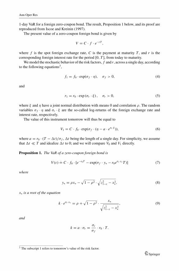
1-day VaR for a foreign zero-coupon bond. The result, Proposition 1 below, and its proof are

reproduced from Iscoe and Kreinin (1997).

The present value of a zero-coupon foreign bond is given by

V = C · f · e−rT ,

where f is the spot foreign exchange rate, C is the payment at maturity T , and r is the

corresponding foreign interest rate for the period [0, T ], from today to maturity.

We model the stochastic behavior of the risk factors, f and r , across a single day, according

to the following equations3,

f1 = f0 · exp(σ f · η), σ f > 0, (4)

and

r1 = r0 · exp (σr · ξ ) , σr > 0, (5)

where ξ and η have a joint normal distribution with means 0 and correlation ρ. The random

variables σ f · η and σr · ξ are the so-called log-returns of the foreign exchange rate and

interest rate, respectively.

The value of this instrument tomorrow will thus be equal to

V1 = C · f0 · exp(σ f · (η − a · eσr ·ξ )), (6)

where a = r0 · (T − �t)/σ f , �t being the length of a single day. For simplicity, we assume

that �t � T and idealize �t to 0; and we will compare V0 and V1 directly.

Proposition 1. The VaR of a zero-coupon foreign bond is

V (ε).= C · f0 · [e−r0T − exp(σ f · y∗ − r0eσr ·x∗ T )] (7)

where

y∗ = ρx∗ −√

1 − ρ2 ·√

z21−ε − x2∗, (8)

x∗ is a root of the equation

k · eσr ·x∗ = ρ +√

1 − ρ2 · x∗√z2

1−ε − x2∗, (9)

and

k = a · σr = σr

σ f· r0 · T .

3 The subscript 1 refers to tomorrow’s value of the risk factor.

Springer

Ann Oper Res

The equation for x∗ will be discussed in the derivation of this result, to which we now

proceed.

Remark: Formally, the 1-factor case of a domestic zero-coupon bond, ( f0 = 1, σ f = 0, ρ =0) is obtained with x∗ = z1−ε.

Proof: For the sake of concreteness, we begin by assuming that ρ > 0, and comment at the

end on the differences in the case that ρ ≤ 0. From the relation (1) we obtain that if

Pr{V0 − V1 > V (ε)} = ε,

then

ε = Pr{η − aeσr ·ξ < �ε},

where

�ε = 1

σ fln

(V0 − V (ε)

f0 · C

).

In order to satisfy the inequality

η − aeσr ·ξ < �ε,

the random vector (ξ, η) equivalently belongs to the region Rε, lying below the curve Lε,

where

Rε = {(x, y) : y − a · eσr ·x < �ε},Lε = {(x, y) : y − a · eσr ·x = �ε}

Necessarily, �ε < 0; otherwise, by inspecting the graph of Lε, we see that

ε = Pr{ (ξ, η) ∈ Rε} > Pr{ξ < 0, η < 0} > 1/4

but ε < 0.1.

The following idea is motivated by Large Deviation Theory. Regard taking a value in Rε

as being extreme or rare. The easiest, most likely way for this to happen is for (ξ, η) to land

in the vicinity of a special point on Lε; namely that point (x∗, y∗) on the joint p.d.f.’s level

curve which is closest to Lε. For our model, the level curves of interest are ellipses with

major axis being the diagonal line: y = x , since ρ > 0.

Finding this point (or a good approximation to it) allows us to determine the value of �ε

and hence V (ε) (or good approximations of them):

V (ε) = V0 − C · f0 · eσ f ·�ε

= C · f0 · [e−r0T − exp(σ f · y∗ − r0eσr ·x∗ T )]. (10)

Clearly, at the special point, the ellipse is tangent to Lε. This imposes only one constraint

on the two unknowns x∗, y∗. To obtain a closed form solution for (10), we will approximate

Springer

Ann Oper Res

T*

Rε

Lε

x

yFig. 1 Region of integration:

case k < ρ

the region Rε with a tangent half-plane (see Figure 1). This will allow us to evaluate the

probability of landing in that region as a function of x∗, y∗. Setting the probability equal to

ε produces the second constraint on x∗, y∗. This approximation of regions is asymptotically

insignificant, as ε tends to 0, as is evidenced by the numerical results of Section 2.1.

We approximate the region Rε with the half-plane Hε = {(x, y) : y < mx + b}, where mand b satisfy y∗ = mx∗ + b, the tangency condition (of the ellipse and Lε):

(x∗ − ρy∗)dx + (y∗ − ρx∗)dy = 0

dy = keσr x∗ dx,

where k = (σr/σ f )rT ; and the probability condition:

ε = Pr{η < mξ + b}

= 1 − �

(b√

m2 − 2ρm + 1

)

where � is the standard normal c.d.f. We can eliminate m and b from these equations as

follows. Dropping the asterisk subscripts, to complete the geometric picture we evidently also

require that m = dy/dx . Substituting m = dy/dx = −(x − ρy)/(y − ρx) and b = y − mxinto the last displayed equation yields, after algebraic simplification,

x2 − 2ρxy + y2 = (1 − ρ2) · z21−ε, (11)

and from the tangency condition

keσr x = − x − ρy

y − ρx. (12)

The final reduction consists in eliminating y from the equations (11) and (12). Note that

y − ρx < 0; otherwise from (12) we would have both

y ≥ ρ−1x and y ≥ ρx

Springer

Ann Oper Res

(we have again used the assumption that ρ > 0), which imply that (x, y) would lie on the

top of the ellipse, i.e., y ≥ x . This is impossible because ε < 1/2. Therefore (11) and (12)

are equivalent to

y = ρx −√

1 − ρ2 ·√

z21−ε − x2 (13)

and

k · eσr ·x = ρ +√

1 − ρ2 · x√z2

1−ε − x2

, (14)

respectively.

Denote

�(x) = x√z2

1−ε − x2

,

so that

k · eσr ·x = ρ +√

1 − ρ2 · �(x).

Obviously,

�(0) = 0,

−∞ = �(−z1−ε) < k · eσr ·(−z1−ε),

and

∞ = �(z1−ε) > k · eσr ·z1−ε .

We also have

� ′(x) = z21−ε

(z21−ε − x2)3/2

> 0,

and the derivative satisfies the conditions � ′(x) ↑ for x > 0, and � ′(x) ↓ for x < 0.

Thus there is a root to equation (14) which can be found numerically. Taking (13) and

(10) into account, concludes the theoretical aspects of our approach to the problem. As for

the numerical aspects, first note that if k = ρ then x = 0 is a root. If k < ρ then graphical

considerations show that there is a unique root x strictly between x− = −ρz1−ε and 0; if

k > ρ, then graphical considerations show that there is a root x strictly between x1 and x2

Springer

Ann Oper Res

0x1−ε

k

ρ

y

x

y=k exp( x)

y=(1- ρ 2)1/2 Ψ ( x ) + ρ

1 2 x x

σ1

-z 1−ε

− z

Fig. 2 Function

ρ + (1 − ρ2)1/2 · �(x)

where

x1 = (k − ρ)z1−ε/√

k2 − 2ρk + 1,

x2 =√

γ

1 + γz1−ε

γ = (k · eσr z1−ε − ρ)2

1 − ρ2.

This last case is illustrated in Figure 2.

Finally we remark that in the case that ρ ≤ 0, the orientation of the ellipses is about

the axis y = −x instead of y = x . The previous derivation goes through with only a small

variation in the argument showing that y∗ − ρx∗ < 0. In case ρ ≤ 0, we would otherwise

have that y∗ ≥ ρx∗ and x∗ < ρy∗ which imply that x∗ = y∗ = 0; which is absurd. �The analytical tractability of the problem for the zero-coupon foreign bond stem from the

two-dimensional nature of the analysis which was further simplified and reduced to a one-

dimensional calculation. As a final example, we indicate a result for a portfolio, �, consisting

of a long position in one zero-coupon bond and a short position in another (both denominated

in the same currency). Using an analysis similar to that in the proof of Proposition 1, we find

the VaR of �, as again we are dealing with only two risk factors.

In the notation of the beginning of this section, the value of the portfolio at time t is given

by

V (t) = C+ · e−r+(T+−t) − C− · e−r−(T−−t)

where C± > 0 are the payments at maturities T± and r± are the corresponding interest rates

for the periods [t, T±], from today until the respective maturities. We let t = 0 correspond to

today and r0± to the interest rates over [0, T±]; V 0 ≡ V (0).

Springer

Ann Oper Res

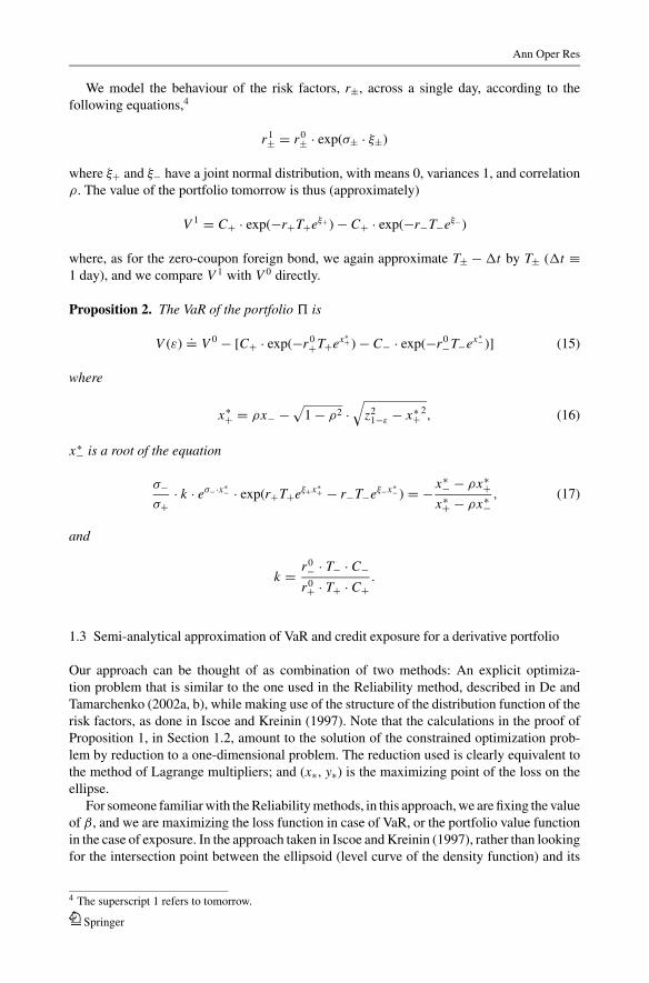
We model the behaviour of the risk factors, r±, across a single day, according to the

following equations,4

r1± = r0

± · exp(σ± · ξ±)

where ξ+ and ξ− have a joint normal distribution, with means 0, variances 1, and correlation

ρ. The value of the portfolio tomorrow is thus (approximately)

V 1 = C+ · exp(−r+T+eξ+ ) − C+ · exp(−r−T−eξ− )

where, as for the zero-coupon foreign bond, we again approximate T± − �t by T± (�t ≡1 day), and we compare V 1 with V 0 directly.

Proposition 2. The VaR of the portfolio � is

V (ε).= V 0 − [C+ · exp(−r0

+T+ex∗+ ) − C− · exp(−r0

−T−ex∗− )] (15)

where

x∗+ = ρx− −

√1 − ρ2 ·

√z2

1−ε − x∗+2, (16)

x∗− is a root of the equation

σ−σ+

· k · eσ−·x∗− · exp(r+T+eξ+x∗

+ − r−T−eξ−x∗− ) = − x∗

− − ρx∗+

x∗+ − ρx∗−, (17)

and

k = r0− · T− · C−

r0+ · T+ · C+.

1.3 Semi-analytical approximation of VaR and credit exposure for a derivative portfolio

Our approach can be thought of as combination of two methods: An explicit optimiza-

tion problem that is similar to the one used in the Reliability method, described in De and

Tamarchenko (2002a, b), while making use of the structure of the distribution function of the

risk factors, as done in Iscoe and Kreinin (1997). Note that the calculations in the proof of

Proposition 1, in Section 1.2, amount to the solution of the constrained optimization prob-

lem by reduction to a one-dimensional problem. The reduction used is clearly equivalent to

the method of Lagrange multipliers; and (x∗, y∗) is the maximizing point of the loss on the

ellipse.

For someone familiar with the Reliability methods, in this approach, we are fixing the value

of β, and we are maximizing the loss function in case of VaR, or the portfolio value function

in the case of exposure. In the approach taken in Iscoe and Kreinin (1997), rather than looking

for the intersection point between the ellipsoid (level curve of the density function) and its

4 The superscript 1 refers to tomorrow.

Springer

Ann Oper Res

tangent coming from the pricing function, we relax the tangency condition and look for the

maximum of the function on the density level curve. This difference of approaches vanishes

when we consider a portfolio of fixed income securities, in which the tangency condition,

defined in Iscoe and Kreinin (1997), corresponds to the maximum of the loss function on

this ellipsoid for fixed income portfolio.

The portfolio value at time t, �t , is expressed as a function of the risk factors R as follows:

�t =N∑

i=1

mivi (R(t)) (18)

where N is the number of instrument in the portfolio, mi is the quantity of the i th instrument

position unit, R(t) is the vector of n risk-factor values at time t , vi is the value of the i th

instrument as a function of the underlying R(t).We can also express the portfolio loss, d�t , as seen at time t over some time horizon, �t ,

as:

d�t ;�t = �t − �t+�t (19)

We assume that the n underlying risk factors are log-normally distributed. The model pa-

rameters are specified by the n-dimensional drift vector μ = (μ1, μ2, . . . , μn) and an n × ncovariance matrix C of the corresponding log-returns. If the current time is t, then the random

value of risk factor i at time t + �t , Ri (t + �t), can be expressed as a function of the current

value of the risk factor, Ri (t), and a set of independent Gaussian risk factors, U1, U2, . . . , Uk ,

as follows:

Ri (t + �t) = Ri (t) exp(μi�t + ξi

√�t) and ξi =

k∑m=1

JimUm (20)

where J is an n × k matrix, (k ≤ n), satisfying C = J ′ J .

Equations (18), (19) and (20) allow us to express the portfolio’s value and its loss as

functions of k standard independent Gaussian risk factors. We define G(·) and G(·) as follows:

G(u1, u2, . . . , uk ; t) :def= �t and G(u1, u2, . . . , uk ; t, �t) :

def= d�t ; �t

The (1 − ε) × 100% credit exposure, E(ε), for time t ′, is the value that satisfies the following

equation:

ε =∫

max(G(u1,... ,uk ;t ′),0)≥E(ε)

�U1,... ,Uk (u1, . . . , uk) du1 · · · duk (21)

Since the region in u-space that will satisfy the inequality

G(u1, . . . , uk ; t ′) ≥ E(ε) is unknown, our approach is to focus on the subregion mak-

ing the major contribution to the integral in (21) and to approximate the boundary of this

region with a tangent hyperplane, passing through the point u = (u1, u2, . . . , uk) that satis-

fies G(u; t ′) = E(ε) instead of using the general formula (21). That is, we approximate the

Springer

Ann Oper Res

(1 − ε) × 100% credit exposure, E(ε), by solving the following optimization problem:

maxu∈Rk

G(u1, u2, . . . , uk ; t ′)

subject to ‖u‖ = �−1(1 − ε) (22)

where �−1(.) is the inverse of the cumulative distribution function of a standard normal

variable. If the solution of the problem is non-negative, then it is the desired credit exposure;

otherwise, the credit exposure is 0.

If one is interested in applying this method to calculate the (1 − ε)% VaR, then one will

have to solve the following optimization problem instead of (22)

maxu∈Rk

G(u1, u2, . . . , uk ; t, �t)

subject to ‖u‖ = �−1(1 − ε)

Very similar to this approach, is the Reliability method. As done in De and Tamarchenko

(2002a), one can consider the following parameterized (by the threshold value, V) optimiza-

tion problem, instead, to calculate β and hence VaR by using equation (3):

minu∈Rk

‖u‖

subject to G(u1, u2, . . . , uk ; t, �t) = V

While the new approach looks similar to the Reliability method’s approach, we believe it is

superior to it because it deals with the following issues:

1. The Reliability methods, as presented in De and Tamarchenko (2002a, b), Kiureghian

(1998), and Madsen, Krunk and Lind (1986), do not use the topological structure of the

distribution of the risk factors in their optimization setup (i.e., they search the whole space

Rn , rather than the hyper-ball, for the design point).

2. In the Reliability method, one computes the probabilities for a range of threshold values

V . While this might be useful to get acquainted with various distribution features, it is an

unnecessary effort if all that interests us is particular quantile (VaR or the credit exposure).

Thus, if there is a unique solution to the problem, the two approaches (semi-analytical

and the Reliability-VaR) will arrive at the correct answer. Points 1 and 2 also have negative

consequences for the performance of Reliability method, in comparaison with our approach.

Indeed, in conjunction with Portfolio Compression, our approach focuses directly on the

correct quantile, rather than solving similar optimization problems for different guesses of

the portfolio loss; and it optimizes over a smaller set.

Note: The optimization problem is not necessarily convex due to the nature of the portfolio

pricing function (see Brandimarte (2002) for further explanation). Thus one utilizes a global

optimization routine, which tends to be more time consuming than the local optimization

routines, to solve (22). As a result, if we are looking for multiple design points, as discussed in

De and Tamarchenko (2002a), then point (1), above, becomes more relevant for the efficiency

of the methods, especially when n is large. For instance, a common approach to global

optimization when the problem is non-convex, is to vary the starting point for the search

algorithm. If we were to use points from a uniform grid, then the number of points needed

to span the whole space grows exponentially with the space dimension. Alternatively, one

Springer

Ann Oper Res

could use quasi-random points based on low discrepancy sequences. It’s known that the upper

bound of the discrepancy of such a sequence is:

DN ≤ C(n) · (lnN )n/N

where n is the dimension of the space, N is the number of points used and C(n) is a constant

that depends on the type of sequence and the dimension (see Jackel (2002) and Sobol (1998)).

Using the above formula, one can show that the number of points needed to maintain a

particular level of discrepancy grows in a non-linear fashion, which justifies the superiority

of our approach to the Reliability one, when the problem is non-convex.

2 Numerical results

In order to test the accuracy of our proposed method, we computed the VaR for a foreign zero-

coupon bond while varying the correlation and volatility of the underlying risk factors, as well

as the desired quantile to verify the applicability of our approach. We compared our results

against the one obtained through Monte Carlo simulation and RiskMetrics methodology. We

also applied our analytical approach to calculate the exposure profile of two portfolios: a

portfolio of fixed income instruments and a portfolio of barrier options. We compared the

profile against the one produced through the Monte Carlo approach to assess the accuracy of

our semi-analytical extension of the results presented in Iscoe and Kreinin (1997).

2.1 Numerical results: Comparison of analytical results with Monte Carlo and

RiskMetrics VaR

Here we compare the accuracy and the performance of our analytical method against VaR

estimation based on an average of several (specifically 10) Monte Carlo simulations, each with

10000 scenarios, and also against RiskMetrics VaR computation (see RiskMetrics (1995)).

The reason for averaging is explained in Iscoe and Kreinin (1996); a hint is provided by

Figure 4. The analysis was done for a foreign zero-coupon bond with a notional value

C = 100; the other parameters were varied and are given below the corresponding graphs.

The parameters in Figure 3 are as follows: f = 1.3, σ f = 0.05, r = 0.056, σr = 0.025,

ρ = 0, T = 1.0. The quantile-probability, p = 1 − ε, varies through the interval [0.89, 0.99].

The relative difference between the Analytical VaR and the RiskMetrics VaR, gets as large

as 5%. The parameters in Figure 4 are as follows: ε = 0.05 (1 − ε = 0.95), f = 1.36,

σ f = 0.05, r = 0.056, σr = 0.023, T = 1.0. The correlation coefficient, ρ, was varied in the

interval (−0.99, 0.99). While the analytical VaR and the Monte Carlo VaR are very close, a

4% relative difference exists between the analytical VaR and the RiskMetrics VaR.

The next two figures represent the behaviour of this function when the volatility parameters

take extremely large values similar to what happened in the Japanese and Mexican markets.

Namely, Figure 5 displays the VaR as a function of the interest rate, r, varied in the interval

(0.05, 0.25). The parameters are as follows: ε = 0.05 (1 − ε = 0.95), f = 2.2, σ f = 0.07,

σr = 0.7, ρ = 0.5, T = 1.0.5 The error of the RiskMetrics approximation is larger than 30%

for wide range of interest rate.

5 We do not display the curve corresponding to the results of Monte Carlo simulation because it is indistin-

guishable from the Analytical VaR curve in Figures 4–5.

Springer

Ann Oper Res

0.9 0.92 0.94 0.96 0.987

8

9

10

11

12

13

14

P

Va

R

RM

Analyt

MC

Fig. 3 VaR computation:

VaR(1 − ε)

0 0.5 19

10

11

12

13

14

15

16

17

18

19

ρ

VaR

(ρ)

RM

Analyt

MC

Fig. 4 Computation of VaR(ρ)

Figure 6 also displays the VaR as a function of the interest rate varied in the interval

(0.05, 0.25) but for higher volatility of interest rate, σr . The parameters are as follows: ε =0.05 (1 − ε = 0.95), f = 2.7, σ f = 0.05, σr = 1.8, ρ = 0.6, T = 1.0. One can observe

that the real behavior of the function VaR(r ) is far away from that of the RiskMetrics

approximation which in addition does not even capture the non-linear shape of the graph of

the function VaR(r ).

Figures 3–6 show that, regardless of the parameters, our analytical approach and the

Monte Carlo method perform similarly for a single zero-coupon foreign bond. On the other

Springer

Ann Oper Res

0 0.05 0.1 0.15 0.2 0.252

2.5

3

3.5

4

4.5

5

5.5

6

6.5

7

r

Va

R(r

)

RM

Analyt

Fig. 5 Value–at–Risk: VaR(r )

0 0.05 0.1 0.15 0.2 0.25 0.3 0.350

50

100

150

200

250

r

Va

R(r

)

RM

Analyt

Fig. 6 Value at Risk: VaR(r )

hand, RiskMetrics approximation is reasonably well behaved (i.e. within 5% difference) for

moderate parameters, σr , ρ and r , but its accuracy degrades as σr or r increases.

2.2 Application of the analytical method for a fixed income portfolio

Having validated the approach against the Monte Carlo method for the case of a zero-coupon

foreign bond, we proceeded to test the method on a portfolio, for exposure profile estimation.

The details of the portfolio (see Table 1) are as follows:

We modelled the dynamics of the four nodes (1-year, 2-year, 3-year, and 4-year) of the

discount curve by a multivariate mean-reverting process. The evolution of these risk factors

Springer

Ann Oper Res

Table 1 Description of portfolioBond 1 Bond 2

Cashflow 160 200

Type zero-coupon zero-coupon

Time to Maturity 3 years 4 years

Position 1 1

Table 2 Parameters of the model1 year 2 years 3 years 4 years

Initial value 7.35% 7.38% 7.396% 8.4%

Level of mean reversion 7.35% 7.38% 7.396% 8.4%

Rate of mean reversion 2 2 2 2

Covariance matrix

1 year 0.04 0.048 0.0512 0.0307

2 year 0.048 0.09 0.096 0.0576

3 year 0.0512 0.096 0.16 0.096

4 year 0.0307 0.0576 0.096 0.09

under this model is described by:

dYi (t) = (θi (t) − αi Yi (t))dt + σi dWi (t), and Yi (0) = Y 0i

where i ∈ {1, 2, 3, 4}, αi > 0 is the rate of mean reversion, θi (t)/αi is the level to which the

risk factor reverts, σi is a positive constant, Wi (t) is a standard Wiener process, and at time

t = 0, the i th risk factor has a known value Y 0i . The details of the model are provided in

Table 2 (The discount rates are simply compounded actual/365 and the variance-covariance

is annualized).

Figure 7, below, shows the results of the analytical estimation of the 99% exposure profile.

If we take the results of the Monte Carlo method as a benchmark for comparison, we find

that the analytical approach captures the credit risk quite accurately (less than 1% error

throughout the life of the portfolio.) In Figure 8, we plotted the portfolio value surface after 1

year as a function of the Gaussian risk factors, and the portfolio value level curve along with

the density level curve that corresponds to a probability of 99%. Note that in Figure 8.b., the

density level curve is for correlated Gaussian variables, and not independent ones as it is for

the remaining figures in this paper. As anticipated, the level curve for the maximum of the

portfolio pricing function is tangent to the density level curve.

2.3 Application of the method to derivative portfolio

We tested our approach by applying it to a portfolio consisting of 2 barrier options. The

currency of the portfolio and of the options is US dollars.6 The details of the portfolio are

given in Table 3:

6 The choice of the currency is arbitrary, and does not change the results of our analysis.

Springer

Ann Oper Res

0 0.5 1 1.5 2 2.5 3 3.5 4200

220

240

260

280

300

320

340

360

Time

Exp

osu

re M

ln $

US

Exposure Estimation

99 % quantile (MC) 99 % quantile (Analyt)

a. 99% Portfolio exposure profile

0 0.5 1 1.5 2 2.5 3 3.5 40

0.1

0.2

0.3

0.4

0.5

0.6

0.7

Time

Re

lative

Err

or

(%)

Exposure Estimation

b. Relative error in 99% exposure estimation

Fig. 7 Exposure profile for a portfolio of fixed income securities

Springer

Ann Oper Res

0

5

0

5

200

250

300

350

Gaussian risk factor 2


Va

lue

220

240

260

280

300

320

340

a. Portfolio value surface as a function of Gaussian variates: U1 and U2

0 0.5 1 1.5 2 2.5

0

1

2

3

4

Portfolio Level Curves


Ga

ussia

n r

isk f

acto

r 2

Density * * *Portfolio Value = 320.91Portfolio Value = 311.28Portfolio Value = 301.94

b. Level curves of portfolio value and density level curve of ξ1 and ξ2,whose raduis square, RHS of Eq. (11), equals to (1− ρ2) · (Φ−1 (0.99))2;

(ε = 0.01)

Fig. 8 Portfolio value surface and level curve for 1-year time horizons

Springer

Ann Oper Res

Table 3 Description of the

portfolio:

Option 1: Up and Out Call,

Option 2: Down and Out Put

Option 1 Option 2

Strike 54 25

Barrier 59 20

Underlying Spot Price 54.2 25

Underlying Volatility 0.1 0.18

Underlying Drift 0.0549 0.0437

Time to Maturity 1 year 1 year

Position 1 1

Discount rate 5.99% 5.99%

Correlation matrix

Stock 1 Stock 2

Stock 1 1 0

Stock 2 0 1

Fig. 9 Comparison results of

Analytical and Monte Carlo

methods

Figure 9 below illustrates the 99% exposure profile obtained through the analytical and

Monte Carlo Methods, (for the Monte Carlo method, we generated 10,000 scenarios of the

risk factors).

For short time horizons, up to 1 month, the analytical method produces results very close

to the one produced with the Monte Carlo method. At the 3-month horizon, we start noticing

a discrepancy, around 10%, and for 3 months before the maturity of the portfolio, the error

becomes as large as 37.6%.

We plotted the portfolio value as a function of the Gaussian factors in Figures 10, 11,

and 12. In the same figure, one will find the level curve of the portfolio value, and the level

density curve corresponding to different probabilities of interest. Inspection of the different

graphs in these figures, reveals the reason for the discrepancy between the results.

For short time horizons, for example 14 days, the portfolio value surface is relatively

flat. Solving the problem setup in (22), we find that the maximum constrained value also

corresponds to the unconstrained maximum value of the surface (Figure 10.a.). We also notice

Springer

Ann Oper Res

01

23

0

1

2

3

0.3

0.4

0.5

0.6

0.7

0.8

0.9

1

Gaussian risk factor 1Gaussian risk factor 2

va

lue

of

po

rtfo

lio

0.35

0.4

0.45

0.5

0.55

0.6

0.65

0.7

0.75

0.8

0.85


0 1 2 3

0

1

2

3


Ga

ussia

n r

isk f

acto

r 2

0.5

0.5

0.7

5

0.75

0.75

0.84849

b. Level curves of portfolio value and density level curves of U1 and U2,whose radius is Φ−1(1 − ε) where (1− ε) ∈ {0.9, 0.99, 0.999}

Fig. 10 Portfolio price surface and level curve for a 14-day time horizon

Springer

Ann Oper Res

0

2

4

0

2

4

0

0.2

0.4

0.6

0.8

1

1.2

1.4

1.6


va

lue

of

po

rtfo

lio

0.2

0.4

0.6

0.8

1

1.2

1.4


0 1 2 3

0

1

2

3


Ga

ussia

n r

isk f

acto

r 2

0.5

0.5

0.5

0.5

0.5

0.5

0.5

0.5

0.5

0.7

5

0.7

5

0.7

5

0.7

5

0.75

0.75

1.0276

1.02

76

1.0

276



Springer

Ann Oper Res

0

1

2

0

1

2

0

0.5

1

1.5

2

2.5

3

3.5

4

4.5


valu

e o

f port

folio

0.5

1

1.5

2

2.5

3

3.5

4


0 1 2 3

0

1

2

3


Gaussia

n r

isk facto

r 2

2

2

2

2

2

2

1.0

276

1.0276

1.0

276

1.0276

1.0

276

1.0276 1.0276

1.0

276

1.0276 1.0276

2.5

287

2.5287

2.5

287

2.5

287

2.5

287

2.5

287

4



Springer

Ann Oper Res

that the level curve whose value is the solution of the optimization problem, is tangent, from

the outside, to the joint density level curve corresponding to a probability of 99%. For this

time horizon, all three analytical methods (Reliability method, the approach taken in De and

Tamarchenko (2002a, b), and this new approach) yield the same results.

For a 182-day horizon, where the error is 30%, we start noticing an interesting feature of

the problem. From Figure 11.b., we see that the level curve, whose value is the solution of the

optimization, is still tangent to the joint density curve corresponding to a probability of 99%,

but this time the tangency is from the inside. That is to say, that all three analytical methods

will yield wrong results, since the level value curve intersects many more density level curves.

Similar behavior is observed when we consider a 330-day time horizon, where the error in

this case is 37%. In Figure 12.b., notice the innermost density level curve corresponding to

80% probability. This curve is tangent to the value level curve, whose value is 4 USD (which

is very close to the Monte Carlo result of 4.02 USD for 99% exposure and not 80%).

2.4 Discussion

From the two applications of the analytical methods to different portfolios, we get conflicting

results: for the case of a fixed income portfolio, the method works exceptionally well. In fact

given that we have an analytical formula for the VaR, in the case of two risk factors, we find

that the analytical results outperform MonteCarlo approach from the computational stand

point.

However, in the case of a derivative portfolio, the semi-analytical approach can fail sub-

stantially (e.g., 37% error). Furthermore, the results are unstable: based on Figure 12.b., we

find that the credit exposure at the 80% confidence interval is larger than the one at 90 and

99%. Having plotted the portfolio value surface and contour levels as functions of the un-

transformed Gaussian risk factors, we conjecture that the following criterion may ensure the

accuracy of the method and is important to understand before using the analytical approach.

For any particular time horizon: the analytical approach will be accurate if the maximum

of the portfolio value, on concentric level density curves, is increasing as a function of

radius, up to the one whose radius is �−1(p); where p is the desired confidence level

of the risk measure.

This criterion means that an extreme movement of risk factors causes extreme change of

the portfolio value. It is satisfied in the case of the fixed income portfolio (see Figure 8), and

for short time horizons, for the derivative portfolio (Figure 10). When we look at the graphs

in situations where the analytical method fails—Figure 12 for instance—we note that the

criterion does not hold: the maximum of the pricing function initially increases as we move

away from the origin, to a value above 4 USD, and then decreases as the radius approaches

the one corresponding to the circle of the 90% level density.

In other words, the analytical (and the semi-analytical) approach relies on the monotonicity

of the maximum (or minimum in the case of VaR) of the portfolio value with respect to the

norm in the risk factor space. In this case, for a given confidence level p0, the tangent

hyperplane at the design point, x∗p0

, separates design points x∗p, p > p0 from R1−p0

. This is

the reason why it outperforms RiskMetrics method, from the accuracy stand point, which

requires the portfolio to be linear with respect to the risk factors, for the results to be exact.

In fact, the reason why RiskMetrics fails drastically, (see e.g., Figure 6), is that in the case

where the volatility is high, a linear approximation of Equation (5), and hence for the portfolio

value, becomes less accurate. Similarly, for high interest rates, the loss of accuracy due to

Springer

Ann Oper Res

the linear approximation of Equation (5) amplifies the truncation error, and results in a poor

approximation of the portfolio VaR.

This criterion provides us with an instance where the analytical method will not work.

Without a rigorous mathematical result, it remains to be researched whether or not there are

other cases where the analytical approximation (or a hybrid of it) may be accurate.

The future research will concentrate on what properties of the portfolio pricing function

will allow us to compute the distribution of exposure (loss in the case of VaR), or even just

an extreme quantile, based on the distribution of risk factor, and on the effects of increasing

the dimension of risk factors space, n.

Although this paper considered the situation where the risk factors can be written as a

function of normal variates, one can work with various distributions of risk factors, in the

manner which is discussed in De and Tamarchenko (2002a).

3 Conclusion

Having studied different methods to calculate Value-at-Risk and a credit exposure profile,

we find that Monte Carlo method remains the most reliable approach to accurately compute

these risk measures. Our analytical method proved to be more accurate than the RiskMetrics

approach to calculate VaR for fixed income securities, and yields results consistent with the

Monte Carlo approach with much less computational effort. We illustrated our analytical

method when the number of risk factors, n, is two. However, it is worth noting that for a large

class of portfolios, it is possible to transform the risk factor space, using possibly non-linear

transformations, to two dimensions (Dembo, Kreinin and Rosen (2001)) and we can apply

the technique developed in Section 1.2.

As a final observation, the semi-analytical method seems to be unreliable when applied

to a simple portfolio of two barrier options. In the case of a portfolio of exotic options,7

application of the semi-analytical methods may lead to a significant error in the estimation

of VaR and exposure profile.

References

Brandimarte, P. (2002). Numerical Methods in Finance—A Matlab Based Introduction.

New York: J. Wiley & Sons.

De, R. and T. Tamarchenko. (2002a). “A New and Accurate Method to Calculate Value at Risk and Other Tail

Measures.” Working paper.

De, R. and T. Tamarchenko. (2002b). “VaR You Can Rely On.” Risk Magazine, 15(8), 77–81.

Dembo, A., J.-D. Deuschel, and D. Duffie. (2004). “Large Portfolio Losses.” Finance and Stochastics, 8, 3–16.

Dembo, A. and O. Zeitouni. (1998). Large Deviation Techniques and Applications, 2nd edition. New York:

Sprinher-Verlag.

Dembo, R., A. Kreinin, and D. Rosen. (2001). “Computer-Implemented Method and Apparatus for Portfolio

Compression.” US patent number: 6,278,981.

Iscoe, I. and A. Kreinin. (1996). “Statistical Analysis of Monte Carlo VaR Estimation.” Technical report,

Algorithmics Inc.

Iscoe, I. and A. Kreinin. (1997). “Analytical Estimations of Value-at-Risk for Fixed Income Securities.”

Technical report, Algorithmics Inc.

Jackel, P. (2002). Monte Carlo Methods in Finance. New York: John Wiley and Sons, LTD.

Jorion, P. (2001). Value at Risk: The New Benchmark for Managing Financial Risk, 2nd edition. New York:

McGraw-Hill.

7 Or a portfolio of simple instruments whose pricing function is equivalent to that of an exotic option.

Springer

Ann Oper Res

Kiureghian, A. (1998). “Multiple Design Points in First and Second-Order Reliability.” Structural Safety,

20(1), 37–49.

Madsen, H., S. Krenk, and N. Lind. (1986). Methods of Structural Safety. New Jersey: Prentice Hall Inc.

RiskMetrics. (1995). RiskMetricsTM-Technical Document. J.P Morgan Guaranty Trust Company, 3rd edition.

http://www.riskmetrics.com/techdoc.html.Sobol, I. (1998). “On Quasi-Monte Carlo Integration.” Mathematics and Computers in Simulation, 47, 103–

112.

Springer

A semi-analytical method for VaR and credit exposure analysis

Documents

Transcript of A semi-analytical method for VaR and credit exposure analysis