Credit Scoring for German Credit Data Project done by Raja K (13MCMB25), Shiva Prasad T (13MCMB16)

under the guidance of

Dr. V.Ravi, Associate Professor, IDRBT

German credit data

Abstract Credit scoring can be defined as a technique that helps credit providers decide

whether to grant credit to consumers or customers. Its increasing importance can be seen

from the growing popularity and application of credit scoring in consumer credit. There are

advantages not only to construct effective credit scoring models to help improve the bottom-

line of credit providers, but also to combine models to yield a better performing combined

model. This paper has two objectives. First, it illustrates the use of data mining techniques to

construct credit scoring models. Second, it illustrates the combination of credit scoring

models to give a superior final model.

Introduction The data set for the illustration is taken from the UCI Machine Learning Repository

[Blake and Merz, 1998]. The data related to a credit screening application in a German bank.

For this two datasets are provided. The original data set, in the form provided by Prof.

Hofmann, contains categorical/symbolic attribute. There are 20 attributes (7 numerical and 13

categorical) and a binary outcome.

For algorithms that need numerical attributes, Strathclyde University produced the file

“german.data-numeric". This file has been edited and several indicator variables added to

make it suitable for algorithms which cannot cope with categorical variables. Several

attributes that are ordered categorical (such as attribute 17) have been coded as integer.

Among the 1000 observations, 700 (or 70.0%) are good credit risk and 300 (30.0%)

are bad credit risk. The 20 attributes available for constructing credit scoring models

including demographic characteristics (e.g., gender and age) and credit details (e.g., credit

history and credit amount)

We want to develop a credit scoring rule that can be used to determine if a new

applicant is a good credit risk or a bad credit risk, based on values for one or more of the

predictor variables.

Problem statement The aim of this project is to construct a model using data mining techniques to

perform credit scoring, is defined as technique that helps credit providers decide whether to

grant credit to customers. Here we are suing German Credit Data Set (source::UCI Machine

Learning Repository), is a classification problem.

Credit Scoring Credit scoring can be formally defined as a statistical (or quantitative) method that is

used to predict the probability that a loan applicant or existing borrower will default or

become fail to pay credit amount. This helps to determine whether credit should be granted to

a borrower or not. Credit scoring can also be defined as a systematic method for evaluating

credit risk that provides a consistent analysis of the factors that have been determined to

cause or affect the level of risk. The objective of credit scoring is to help credit providers

quantify and manage the financial risk involved in providing credit so that they can make

better lending decisions quickly and more objectively.

Benefits of Credit Scoring

Increased Credit Availability

The use of credit scores gives lenders a much better understanding of risk than

previously, giving them the confidence to offer credit to more people. Lenders who

use credit scoring can approve more loans, because credit scoring gives them more

information upon which they can base their decisions to make loans. In addition,

lenders can tailor a range of loans to different risk levels and offer a whole range of

credit options.

Lower Credit Rates

With more credit available the cost of credit for borrowers has decreased. Automated

credit processes, including credit scoring, make the credit process more efficient and

thus less costly for lenders, who pass savings on to their customers. In addition,

lenders can more effectively control their losses using credit scoring systems, again,

allowing them to offer lower overall rates.

Fairer Credit Decisions

Credit scoring is an automated mathematical process that utilizes technology to

determine suitability for loans. It considers only factors related to credit risk,

removing from the lending process the risk of human bias based on race, religion

nationality or marital status.

Faster Credit Decisions

Technology that utilizes scoring systems allows lenders to make instant credit

decisions. This is notable in virtually all areas where a consumer seeks credit, from a

retail store to an auto dealership to buying a home. In the personal loan and mortgage

lending industry, applications can be approved in hours rather than weeks for

borrowers who score above a lender's score cut-off.

Opportunities to Improve Credit Rating

Before the advent of credit scoring, so-called “knock out rules” meant that lenders

often turned away borrowers based on a past problem in their file. Credit scoring

considers all credit-related information, good and bad, in a person’s credit report.

With credit scoring systems past credit problems fade as time passes and as recent

good payment patterns are established.

Applications of Credit Scoring

TOOLS USED

KNIME

WEKA

Techniques Used

Support Vector Machine

Decision Tree

Logistic regression

Multilayer Perceptron

RProp Multilayer Perceptron

Probabilistic Neural Network

Variable Description

Var.# Variable name Variable type Variable type

1 OBS# Categorical Observation No.

2 CHK_ACCT Categorical Checking account status

3 DURATION Numerical Duration of credit in months

4 HISTORY Categorical Credit history

5 NEW_CAR Binary Purpose of credit

6 USED_CAR Binary Purpose of credit

7 FURNITURE Binary Purpose of credit

8 RADIO/TV Binary Purpose of credit

9 EDUCATION Binary Purpose of credit

10 RETRAINING Binary Purpose of credit

11 AMOUNT Numerical Credit amount

12 SAV_ACCT Categorical Average balance in savings account

13 EMPLOYMENT Categorical Present employment since

14 INSTALL_RATE Numerical Instalment rate as % of disposable

income

15 MALE_DIV Binary Applicant is male and divorced

16 MALE_SINGLE Binary Applicant is male and single

17 MALE_MAR_WID Binary Applicant is male and married or a

widower

18 CO-APPLICANT Binary Application has a co-applicant

19 GUARANTOR Binary Applicant has a guarantor

20 PRESENT_RESIDENT Categorical Present resident since - years

21 REAL_ESTATE Binary Applicant owns real estate

22 PROP_UNKN_NONE Binary Applicant owns no property (or

unknown)

23 AGE Numerical Age in years

24 OTHER_INSTALL Binary Applicant has other instalment plan

credit

25 RENT Binary Applicant rents

26 OWN_RES Binary Applicant owns residence

27 NUM_CREDITS Numerical Number of existing credits at this bank

28 JOB Categorical Nature of job

29 NUM_DEPENDENTS Numerical Number of people for whom liable to

provide maintenance

30 TELEPHONE Binary Applicant has phone in his or her

name

31 FOREIGN Binary Foreign worker

32 RESPONSE Binary Credit rating is good

Model Description

Decision Tree (DT): The decision tree is a structure that includes root node, branch and leaf node. Each

internal node denotes a test on attribute, each branch denotes the outcome of test and each

leaf node holds the class label. The topmost node in the tree is the root node.

The decision making can be either nominal or numerical.

Numeric splits are always binary (two outcomes), dividing the domain in two

partitions at a given split point.

Nominal splits can be either binary (two outcomes) or they can have as many

outcomes as nominal values.

In the case of a binary split the nominal values are divided into two subsets. The algorithm

provides two quality measures for split calculation; the gini index and the gain ratio. Further,

there exist a post pruning method to reduce the tree size and increase prediction accuracy.

The pruning method is based on the minimum description length principle.

The algorithm can be run in multiple threads, and thus, exploit multiple processors or cores.

Advantages:

It does not require any domain knowledge.

It is easy to assimilate by human.

Learning and classification steps of decision tree are simple and fast.

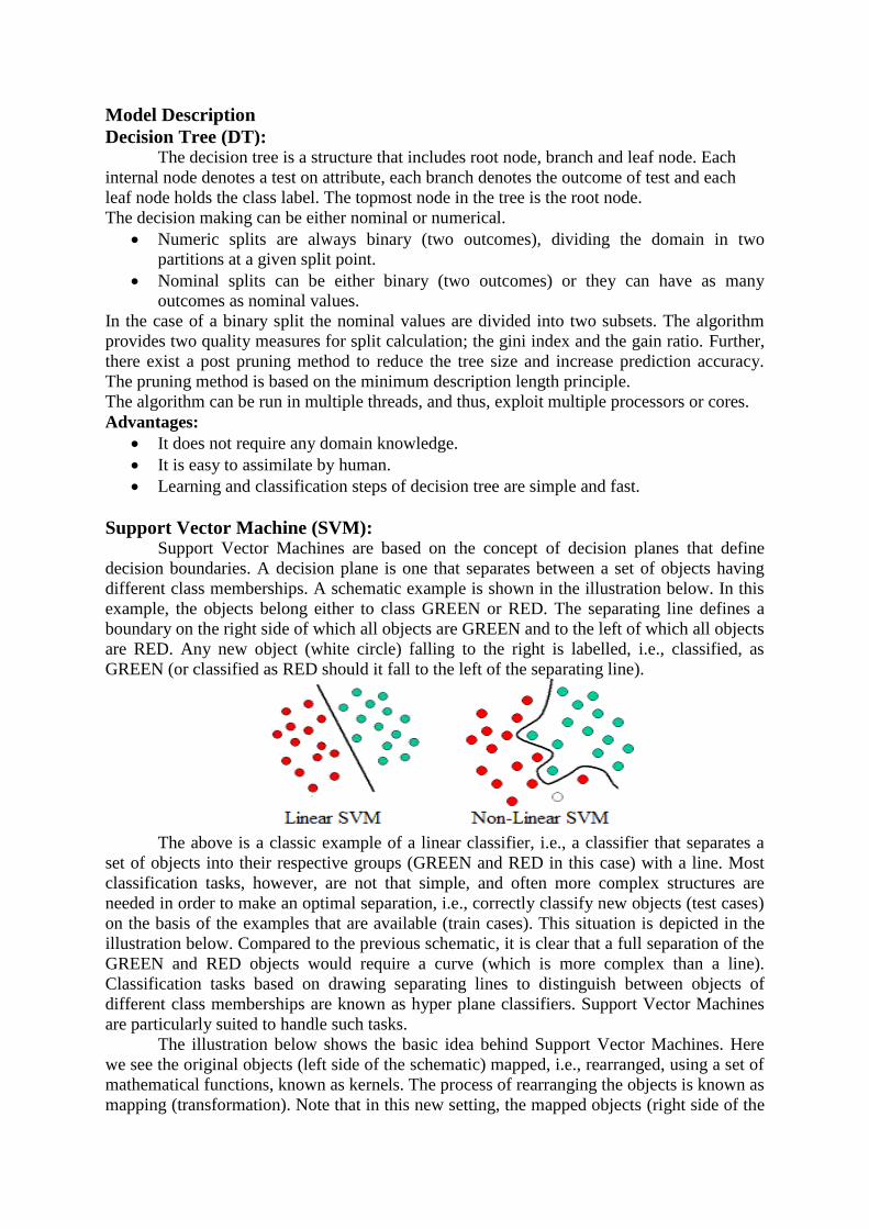
Support Vector Machine (SVM): Support Vector Machines are based on the concept of decision planes that define

decision boundaries. A decision plane is one that separates between a set of objects having

different class memberships. A schematic example is shown in the illustration below. In this

example, the objects belong either to class GREEN or RED. The separating line defines a

boundary on the right side of which all objects are GREEN and to the left of which all objects

are RED. Any new object (white circle) falling to the right is labelled, i.e., classified, as

GREEN (or classified as RED should it fall to the left of the separating line).

The above is a classic example of a linear classifier, i.e., a classifier that separates a

set of objects into their respective groups (GREEN and RED in this case) with a line. Most

classification tasks, however, are not that simple, and often more complex structures are

needed in order to make an optimal separation, i.e., correctly classify new objects (test cases)

on the basis of the examples that are available (train cases). This situation is depicted in the

illustration below. Compared to the previous schematic, it is clear that a full separation of the

GREEN and RED objects would require a curve (which is more complex than a line).

Classification tasks based on drawing separating lines to distinguish between objects of

different class memberships are known as hyper plane classifiers. Support Vector Machines

are particularly suited to handle such tasks.

The illustration below shows the basic idea behind Support Vector Machines. Here

we see the original objects (left side of the schematic) mapped, i.e., rearranged, using a set of

mathematical functions, known as kernels. The process of rearranging the objects is known as

mapping (transformation). Note that in this new setting, the mapped objects (right side of the

schematic) is linearly separable and, thus, instead of constructing the complex curve (left

schematic), all we have to do is to find an optimal line that can separate the GREEN and the

RED objects.

Multilayer perceptron (MLP):

A multilayer perceptron (MLP) is a feed forward artificial neural network model

that maps sets of input data onto a set of appropriate outputs. A MLP consists of multiple

layers of nodes in a directed graph, with each layer fully connected to the next one. Except

for the input nodes, each node is a neuron (or processing element) with a nonlinear activation

function. MLP utilizes a supervised learning technique called back propagation for training

the network. MLP is a modification of the standard linear perceptron and can distinguish data

that are not linearly separable. Based on a trained Multilayer Perceptron-model given at the model, the expected output

values are computed. If the output variable is nominal, the output of each neuron and the class of the winner neuron are produced. Otherwise, the regression value is computed. Filter out missing

values before using this node.

Activation function:

If a multilayer perceptron has a linear activation function in all neurons, that is, a linear

function that maps the weighted inputs to the output of each neuron, then it is easily proved

with linear algebra that any number of layers can be reduced to the standard two-layer input-

output model. What makes a multilayer perceptron different is that each neuron uses

a nonlinear activation function which was developed to model the frequency of action

potentials, or firing, of biological neurons in the brain. This function is modelled in several

ways.

The two main activation functions used in current applications are both sigmoid, and are

described by

Layers:

The multilayer perceptron consists of three or more layer of nonlinearly-activating nodes.

Each node in one layer connects with a certain weight to every node in the following

layer. Some people do not include the input layer when counting the number of layers and

there is disagreement about whether should be interpreted as the weight from i to j or the

other way around.

Logistic Regression (LR): Logistic regression predicts the probability of an outcome that can only have two values (i.e.

a dichotomy). The prediction is based on the use of one or several predictors (numerical and

categorical). A linear regression is not appropriate for predicting the value of a binary

variable for two reasons:

A linear regression will predict values outside the acceptable range (e.g. predicting

probabilities outside the range 0 to 1).

Since the dichotomous experiments can only have one of two possible values for each

experiment, the residuals will not be normally distributed about the predicted line.

On the other hand, a logistic regression produces a logistic curve, which is limited to values

between 0 and 1. Logistic regression is similar to a linear regression, but the curve is

constructed using the natural logarithm of the “odds” of the target variable, rather than the

probability. Moreover, the predictors do not have to be normally distributed or have equal

variance in each group.

In the logistic regression the constant (b0) moves the curve left and right and the slope (b1)

defines the steepness of the curve.

Probabilistic Neural Network (PNN): Probabilistic Neural Network (PNN) based on the DDA (Dynamic Decay

Adjustment) method on labelled data using Constructive Training of Probabilistic Neural

Networks as the underlying algorithm.

This algorithm generates rules based on numeric data. Each rule is defined as high-

dimensional Gaussian function that is adjusted by two thresholds, theta minus and theta plus,

to avoid conflicts with rules of different classes. Each Gaussian function is defined by a

centre vector (from the first covered instance) and a standard deviation which is adjusted

during training to cover only non-conflicting instances. The selected numeric columns of the input

data are used as input data for training and additional columns are used as classification target, either one column holding the class information or a number of numeric columns with class degrees

between 0 and 1 can be selected. The data output contains the rules after execution along with a number of rule measurements. The model output port contains the PNN model, which can be used

for prediction in the PNN Predictor node.

Rprop Multilayer perceptron (Rprop MLP): Rprop, short for resilient back propagation, is a learning heuristic for supervised

learning in feed forward artificial neural networks. This is a first-

order optimization algorithm.

Rprop takes into account only the sign of the partial derivative over all patterns (not

the magnitude), and acts independently on each "weight". For each weight, if there was a sign

change of the partial derivative of the total error function compared to the last iteration, the

update value for that weight is multiplied by a factor η−, where η− < 1. If the last iteration

produced the same sign, the update value is multiplied by a factor of η+, where η+ > 1. The

update values are calculated for each weight in the above manner, and finally each weight is

changed by its own update value, in the opposite direction of that weight's partial derivative,

so as to minimise the total error function. η+ is empirically set to 1.2 and η− to 0.5.

Basic Data mining method

Input Data:

Here we are giving the data as input to the classifier after data cleaning process.

Classification:

Classification consists of assigning a class label to a set of unclassified cases.

.Supervised Classification

The set of possible classes is known in advance.

Unsupervised Classification

Set of possible classes is not known. After classification we can try to assign a

name to that class. Unsupervised classification is called clustering.

Classification methods:

Genetic Algorithms

Rough Set Approach

Fuzzy Set Approaches

Building Model:

Building a mining model is part of a larger process that includes everything from

asking questions about the data and creating a model to answer those questions, to deploying

the model into a working environment.

A model may be either opaque (it works but we aren't exactly sure how or why) or

transparent (we understand exactly how the model arrives at any prediction). Either may be

acceptable, depending upon the application. An opaque model that predicts production defect

rates is perfectly acceptable if our interest is limited to production planning, but we would

certainly prefer a transparent model if we were interested in increasing productivity.\

Testing Data Set:

We have to compare the predictions to the known answers. Data is also known as test

data or evaluation data. This technique is called testing a model, which measures the model's

predictive accuracy.

Results: The results those we have achieved after comparing the data with learned knowledge data by

the model.

Results

S.NO. Model Sensitivity (%) Specificity (%) Accuracy (%)

1 Support Vector Machine + PCA 87.85714286 43.333333 74.5

2 Decision Tree 86.66666667 44.615384 73

3 Logistic regression 92.14285714 51.666666 80

4 Multilayer Perceptron 85.50724638 32.258064 69

5 Probabilistic Neural Network 92.85714286 23.333333 72

6 Rprop Multilayer Perceptron 85.15625 50 72.5

Comparing Models Using ROC curve (Hold-Out results)

Using ROC curve (10 Fold Cross validation)

Using T-Test (based on sensitivity)

Comparing T-Test Comparing T-Test

LR vs DT 3.5 SVM vs DT 14.2

LR vs MPL 12.5 SVM vs MLP 15.4

LR vs SVM 19.06 SVM vs PNN 4.9

LR vs PNN 7.88 SVM vs Rprop 22.6

LR vs Rprop 14.40 SVM vs LR 19.06

Using T-Test (based on Accuracy)

Comparing T-Test

LR vs DT 1.225

LR vs MPL 4.42

LR vs SVM 3.586

LR vs PNN 3.82

LR vs Rprop 2.1

Conclusion This paper discusses and illustrates the use of data mining techniques in the

construction and combination of credit scoring models.

LR gave better results than other models.

According to the T-Test based on the accuracy LR, DT and Rprop MLP significantly

same.

According to the T-Test based on the accuracy LR, SVM and PNN significantly not

same

So according to the ROC curve and accuracy statics we can prefer LR model

.

References

A Two-step Method to Construct Credit Scoring Models with Data Mining

Techniques published in International Journal of Business and Information Volume 1

Number 1, 2006 pp 96-118 by Hian Chye Koh,Wei Chin Tan,Chwee Peng Goh

Guide to Credit Scoring in R by DS (ds5j@excite.com) (Interdisciplinary Independent

Scholar)

Credit scoring with a data mining approach based on support vector machines from

the Expert Systems with Applications by Cheng-Lung Huang, Mu-Chen Chen, Chieh-

Jen Wang

Credit scoring in banks and financial institutions via data mining techniques: A

literature review By Seyed Mahdi sadatrasoul ,Mohammadreza

gholamian,Mohammad Siami,Zeynab Hajimohammadi