Prediction of loan defaults using a credit card scoring model

incorporating worthiness

Francisco Camões Manuela Magalhães Hillfhcc@iscte.pt mmmh@iscte.pt

Department of Economy Department of Quantitative MethodsUNIDE - I.S.C.T.E. – PORTUGAL

Abstract

The prediction of loan defaults has been the basis of a growing interest in the

development of systems of credit scoring. Typically, discriminant analysis, probit, logit, or

some other type of classificatory procedure has then been applied to develop a model for

distinguishing between “good” and “bad” payers. However, some published studies have

concluded that the use of models that seek to minimise misclassification errors do not

necessarily lead to an increase in the credit concession profits.

In this paper two approaches for the inclusion of worthiness in credit card scoring

models were investigated. In the first of these, worthiness was added to the usual credit

scoring models, while in the second it formed the basis of a new methodology. Evidence was

obtained that “good payers” are not necessarily “good customers” of credit card companies,

and this is a major conclusion with clear implications for choosing the best model.

Keywords: Credit scoring; Probit; Two step estimation.

1. Introduction

The prediction of loan defaults has an obvious practical utility. Indeed, the

identification of default risk appears to be of special interest to loan providers and,

since the nineteen sixties, has been the basis of a growing interest in the U.S.A. in the

development of systems of credit scoring by companies granting consumer credit.

Due to their proprietary nature little is known about the specific content and

structure of credit scoring models, however, a relatively large number of studies have

been published on such models1. Typically, these have been based upon a sample of

credits or loans that had received prior approval. Discriminant analysis, multiple

linear regression, probit, logit or some other type of classificatory procedure has then

been applied to develop a model for distinguishing between “good” and “bad” payers.

In published studies, transformations of the independent variables have been

used to overcome problems of non-normality in the distributions of the original

variables and (or) to establish monotonic relationships between these and the

proportion of good customers2. Attention has also been paid to the fact that the

distributions of “bad” and “good” payers could hardly be considered symmetrical3.

On the other hand, some studies have concluded that the use of models that seek to

minimise misclassification errors do not necessarily lead to an increase in the credit

concession profits4.

On the basis of the above points, an attempt was made to construct an

acceptance credit scoring model for credit cards using the techniques of linear

discriminant analysis (D), logit (L), probit (P), gombit (G) and weibit (W)5. Thus, in

addition to a linear discriminant analysis, models were developed based on two

symmetrical accumulated distributions of probability (normal and logistic) and two

asymmetric accumulated distributions of probability (Weibull and Gompertz6). These

models were estimated based not only on original variables (o), but also on

transformations of these variables by weight of evidence (e) and reduction of classes

of weight of evidence in order to establish a monotonic relation with proportions of

“good” payers were used (m) 7.

The data set used for estimation and validation consisted of 5281 cardholders

randomly stratified by month of acquisition of the credit card (April of 1994 to May

of 1995) and embracing a span of 14 months of use (January of 1995 to February of

1996). This sample was provided by a Portuguese financial institution.

For each individual the usual socio-demographic characteristics (age, type of

dwelling, marital status etc.) were recorded6. The following monthly data relating to

the use of the credit card were also recorded: number of purchases, amount of debt at

the end of the month, the value of payments made by bank transfer, the situation

regarding payments not made and /or cancellation of the card.

1 See Rosenberg & Gleit (1994).2 Boyle & All (1992) e Banasik & All (1996).3 Clark & McDonald (1992).4 Boyes & All (1989), Clark & McDonald (1992 e Greene (1992).5 Camões & Hill (2000).6 The formulation proposed by Aldrich & Nelson (1984, pp.87) for the Gompertz accumulated

distribution of probability ( ( )bxe

xy eP−−

= =1 ) was adopted.7 See Tables A-1 and A-2

The entire sample was randomly divided into two sub-samples - a construction

sample of 3961 cases and a validation sample of 1320 cases (25%). A customer with

two or more months of payments in arrears was considered a “bad” payer. Under this

definition there were 445 “bad” payers (8,43%) - 334 of whom were in the

construction sample and 111 were in the validation sample.

Several models were estimated with the dependent variable coded as 0 for

“bad” payers and 1 for “good” payers. For the weibit8 model the formulation

presented by Greene (1995, p. 437) was adopted, and the same one was adapted for

the gombit9 model – by substitution of the accumulated probability distribution.

The first estimated models, based on the original variables presented evidence

of serious multicollinearity. After reducing multicolinearity, hetroscedasticity with

the specification Var[ε]2zÄe

′= , suggested by Greene10, was incorporated.

The incorporation of this form of heteroscedasticity produced some problems,

namely:

• Greater standard errors;

• Reversed coefficient signs among models;

• Reversal of signs from the coefficients to the marginal effects for some

variables.

In spite of all that, is was found that the predictive capacity of the different

estimated models is very similar and also similar to that achieved by just assuming

that all costumers are “good” payers11.

Thus, the aim of this paper is invetigate how to incorporate customer

acceptance worthiness, not only to assist in discovering which is the best model but

also to test whether a “good payer” is a “good customer” or not.

8 Prob[ 1=iy ]

ixeeβ ′−−=1

9 Prob[ 1=iy ]ixee

β ′−−=10 Greene, 1995, pp.42511 See Annex 1

2. Incorporating expected worthiness

If we admit that the expenditures, after deduction of the respective commission,

are paid to the merchants in the same month, and defining:

a = open account cost minus card fee

b = transaction cost, equal to the month cost

of open account

c = merchant fee

d = month finance charge on debt

e = month card expenditure

f = month receipts

g = month discount rate

h = month transactions number

j = month debited interest

p = probability of debt income

The present value of what can be designated by contribution margin for profits (MC0)

in a period of I months is given by:

( )

( ) ( )

( )( ) ( )

( ) ( ) 11

11

10

11

11

1

1

1 +=

+=

= +−

+×−++×−−

+

−+×+

×++

= ∑∑

∑ I

I

ii

iiI

I

iiiI

ii

i

g

b

g

echba

g

fjed

pg

fMC

where

( )∑= +

I

ii

i

g

f

1 1 = present value of receipts;

( ) ( )

( ) 1

1

1

1

+=

+

−+×+

×∑

I

I

iii

g

fjed

p = expected present debt value at the end

of the considered period;

( ) ( )( )∑

= +×−++×I

ii

ii

g

echb

1 1

11 = present costs value of open account and

payments of cards expenditures;

( ) 11 ++ Ig

b = present costs value of open account in the period I+1.

Based on the definitions presented above we have:

( )( ) ( )

( ) ( )∑∑=

+= +

−+

×−++×−−

+

I

iIi

iiI

ii

i

g

b

g

echba

g

f

11

1 11

11

1 = present net value of

receipts;

( ) ( )

( ) 1

1

1

1

+=

+

−+×+ ∑

I

I

iii

g

fjed = present debt value.

Because the minimum period for communication of non-renewal of the credit

card is normally one month, the reference period for making a decision about the first

renewal of the card, is 9 months.

Because a part of the data required was not available, some approximations

were used. It was assumed that cards receipts were equal to the transferred values,

and that the debits made to customers for whom there were no reported expenditures

were financial charges. It was also assumed that: a=2000; b=100; c=0,02; d=0,02 and

g=0,005.

On the basis of these assumptions it was possible to calculate present debt

values, present value of receipts minus payments and costs value concerning the first

9 months of card usage. Tables 1 and 2 present a statistic description for all

customers for whom the necessary data were available (1872). Of this number 1393

belonged to the construction sub-sample and 479 to the validation sub-sample.

Table 1 - present value of receipts minus payments and costs value (first 9 months)

(escudos)Total sample Construction

SampleValidation

sampleMean -23.689,05 -23.211,81 -25.076,93Median -877,89 -877,89 -877,89Mode -877,89 -877,89 -877,89Standard deviation 42.217,53 42.645,82 40.958,64Range 320.075,37 320.075,37 268.359,61Minimum -298.790,31 -298.790,31 -256.201,60Maximum 21.285,06 21.285,06 12.158,00Sum -44.345.907,99 -32.334.054,16 -12.011.853,83Number of cases 1.872 1.393 479

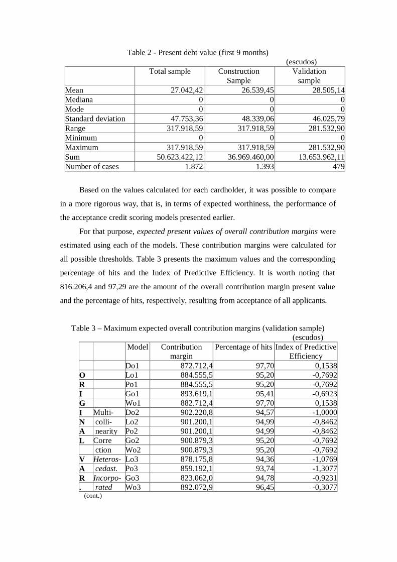
Table 2 - Present debt value (first 9 months)(escudos)

Total sample ConstructionSample

Validationsample

Mean 27.042,42 26.539,45 28.505,14Mediana 0 0 0Mode 0 0 0Standard deviation 47.753,36 48.339,06 46.025,79Range 317.918,59 317.918,59 281.532,90Minimum 0 0 0Maximum 317.918,59 317.918,59 281.532,90Sum 50.623.422,12 36.969.460,00 13.653.962,11Number of cases 1.872 1.393 479

Based on the values calculated for each cardholder, it was possible to compare

in a more rigorous way, that is, in terms of expected worthiness, the performance of

the acceptance credit scoring models presented earlier.

For that purpose, expected present values of overall contribution margins were

estimated using each of the models. These contribution margins were calculated for

all possible thresholds. Table 3 presents the maximum values and the corresponding

percentage of hits and the Index of Predictive Efficiency. It is worth noting that

816.206,4 and 97,29 are the amount of the overall contribution margin present value

and the percentage of hits, respectively, resulting from acceptance of all applicants.

Table 3 – Maximum expected overall contribution margins (validation sample)(escudos)

Model Contributionmargin

Percentage of hits Index of PredictiveEfficiency

Do1 872.712,4 97,70 0,1538O Lo1 884.555,5 95,20 -0,7692R Po1 884.555,5 95,20 -0,7692I Go1 893.619,1 95,41 -0,6923G Wo1 882.712,4 97,70 0,1538I Multi- Do2 902.220,8 94,57 -1,0000N colli- Lo2 901.200,1 94,99 -0,8462A nearity Po2 901.200,1 94,99 -0,8462L Corre Go2 900.879,3 95,20 -0,7692

ction Wo2 900.879,3 95,20 -0,7692V Heteros- Lo3 878.175,8 94,36 -1,0769A cedast. Po3 859.192,1 93,74 -1,3077R Incorpo- Go3 823.062,0 94,78 -0,9231. rated Wo3 892.072,9 96,45 -0,3077

(cont.)

Table 3 – Maximum expected overall contribution margins (validation sample)(escudos)

(cont.)Model Contribution

marginPercentage of hits Index of Predictive

EfficiencyW. De1 873.432,4 88,73 -3,1539E Le1 867.726,8 96,03 -0,4615V Pe1 855.532,3 96,87 -0,1539I Heteros- Le2 867.726,8 96,03 -0,4615D. cedast. Pe2 867.726,8 96,03 -0,4615M Dm1 852.153,6 92,48 -1,7692O Lm1 852.563,3 96,45 -0,3077N Pm1 853.441,2 96,24 -0,3846O Gm1 852.563,3 96,45 -0,3077T Wm1 853.441,2 96,24 -0,3846O Heteros- Lm2 888.511,5 82,88 -5,3077N cedast. Pm2 917.762,4 83,72 -5,0000I Incorpo- Gm2 883.089,0 84,34 -4,7692C rated Wm2 885.262,1 83,51 -5,0769

In order to gain insight about the variability of the estimates, 1.000 bootstrap

samples where computed. The resulting mean, standard deviation and 95%

confidence interval (based on the modified percentile method) are presented in Table

4.

Table 4 – Mean, standard deviation and 95% confidence interval limits(1000 bootstrap samples)

Model Meancontribution

margin

Standarddeviation

95% confidence interval

Lower limit Upper limitO Do1 874.704,6 215.934,9 414.935,3 1.261.546,0R Lo1 882.538,8 206.548,0 474.496,7 1.280.340,0I Po1 869.208,9 206.709,2 447.763,1 1.248.705,5G Go1 890.968,0 206.897,9 472.909,2 1.283.822,5I Wo1 879.933,8 215.981,5 436.298,9 1.284.210,5N Multi- Do2 900.007,2 207.423,7 474.699,6 1.286.854,0A colli- Lo2 893.114,7 207.802,8 502.124,5 1.313.654,0L nearity Po2 899.052,9 207.426,8 477.585,5 1.290.442,5

Corre Go2 892.798,1 207.818,6 501.964,1 1.313.493,5V ction Wo2 892.798,1 207.818,6 501.964,1 1.313.493,5A Heteros- Lo3 864.591,5 206.423,9 464.062,8 1.249.402,5R cedast. Po3 853.046,4 204.933,6 434.005,0 1.245.734,5. Incorpo- Go3 803.751,7 214.783,4 365.019,7 1.201.490,0

rated Wo3 883.078,8 206.624,2 465.804,7 1.260.859,0(cont.)

Table 4 – Mean, standard deviation and 95% confidence interval limits(1000 bootstrap samples)

(cont.)Model Mean

contributionmargin

Standarddeviation

95% confidence interval

Lower limit Upper limitW. De1 869.039,8 191.140,2 510.845,9 1.261.456,5E Le1 852.771,6 208.846,5 456.641,8 1.272.700,0V Pe1 848.312,4 215.362,2 410.013,2 1.245.870,5I Heteros- Le2 847.386,8 208.612,7 438.916,7 1.245.207,5D. cedast. Pe2 860.462,1 209.189,0 425.548,5 1.244.606,0M Dm1 850.421,6 205.588,8 462.494,2 1.254.277,5O Lm1 847.628,1 212.673,2 444.345,2 1.271.121,0N Pm1 848.563,6 212.626,2 445.662,0 1.271.592,0O Gm1 847.691,8 212.676,8 444.345,2 1.271.153,0T Wm1 847.052,6 212.650,7 444.138,9 1.270.765,0O Heteros- Lm2 884.532,0 137.222,7 661.686,3 1.189.890,5N cedast. Pm2 901.628,9 138.691,2 643.642,3 1.169.196,0I Incorpo- Gm2 875.400,6 146.875,4 620.457,3 1.177.128,0C rated Wm2 829.402,2 148.570,9 560.205,6 1.138.549,5

In brief the results just presented show:

• All models lead to maximum expected contribution margins greater then

the ones resulting from acceptance of all applicants;

• Almost all models, with the exception of discriminant and weibit

models based on original variables, show a conflict between seeking

best profits and minimizing misclassifications;

• There are no great differences between maximum contribution margins

obtained with estimated models based on the same kind of variables.

The major differences occur between models incorporating

heteroscedasticity;

• The lower variability in models incorporating hateroscedasticity based

on transformed variables in order to establish a monotonic relationship

with “good” payers proportion.

3. A worthiness credit scoring model

The previous exercise supports the thesis that using a credit scoring model

based on the implicit assumption that bad payers are bad customers can lead to the

choice of a threshold that is not compatible with an increase in expected profits. In

fact, not all customers who are good payers are good customers, so the definition of a

threshold that minimises misclassification of customers in terms of payments owed,

does not lead to the largest value of expected profits.

Thus, starting from the evidence that a customer can only contribute to profits

if his present value of contribution margin is positive, that is, if present value of

receipts plus present value of debt at the end of the evaluation period is positive, we

tried to model:

• The present value of net receipts (RECBL0) as a function of the

customers' characteristics;

• The present value of debt (VADIV0) as a function of the

customer’s characteristics and present value of net income.

On the other hand, the positive contribution to profits from customers depends

on the expected contribution margin, that is, on the present value of net receipts plus

the expected present value of debt - that naturally depends of the customers' quality in

terms of the payments owed. But, this "quality" also depends on the amount of the

debt and thus the complete model to estimate will also include:

• The customer's payments “quality" (Po4) as a function of his

characteristics and present value of debt.

Since there is a qualitative dependent variable in the model, this was estimated

based on the 1393 costumers of the construction sample already difined.

There are 57 “bad” payers in the total sample, of which 44 were in the

construction sample and 13 in the validation sample, representing proportions of

0,03045, 0,03159 and 0,02714 respectively.

The complete model was estimated using the software LIMDEP in two phases.

The first two functions were estimated using the three stage least squares method,

and subsequently a two step estimation of a probit model with a regressor estimated

in the first phase (present value of final debt), was carried out. This phase was based

on a program presented by Greene (1988)12 that incorporates the asymptotic

covariance matrix formulation difined by Murphy and Topel13.

The model was estimated based on the original variables. Given the serious

multicollinearity, exogeneous variables that had the smallest t-ratio where throwed

12 The program “Two Step Estimation of Probit with Estimated Regressor” presented in the Help File .Also in www.limdep.com/On_Line_Help/lim00464.htm.13 Theorem 10.3 in Greene (2000 p. 433-4).

out, in succession, until the condition index of the cross-product matrix reached a

value under 20.

Tables 5 to 8 present the estimated models where, besides the variables already

presented, we have:

Variable DescriptionRECBL0 Present value of net receipts (9 months)VADIV 0 Present value of debt (9 months)ESTDIV VADIV 0 estimateESTREC RECBL0 estimatePO4 “Good” payer estimate (probability)

Table 5 – RECBL0 equation

Variable CoefficientStandar error

Constant -20319,016463345,0116

NAPROF 11534,347162659,0210

ANTCBAN 635,34445363,83046

ANTHAB 90,65355115,48419

ANTHABA -2410,09383924,39004

CARTOESC -7741,487772672,2600

COU -3781,041754888,3994

CTERMO 3876,501966898,7643

HABA -1322,791342857,8450

HABF -10543,217814003,2919

NEET 1648,421344196,0420

NRFILHOS -1199,192001319,7944

NNRF -10524,916723145,7942

NRPES -3659,232791271,7527

SFD -17123,524644364,6859

ENCT -118,8103454,05996

AB2 -11,3019610,36791

AHA2 70,4029237,92022

RE2 -0,020670,01837

R2 = 0,0946R2 adjust. = 0,0827F(18, 1374) = 7,97, Prob. V. = 0,0000

Table 6 – VADIV0 Equation

Variable CoefficientStandar error

Constant 3090,753731568,1471

NAPROF -1349,7684969,71568

ANTCBAN -167,6311885,04182

ANTHAB -40,7255725,17532

ANTHABA -28,705989,6595

COUTP -1380,67497498,67525

COU -639,708671060,7995

CTERMO -701,017511506,3848

HABA 782,42947607,50490

HABF 552,436181078,5057

NEET -280,317622893,05895

NRFILHOS -388,37872298,36485

NNRF -892,79273935,18984

NRPES 459,90757349,63305

SFD -392,859891429,0495

ENCT 5,2963914,23135

AB2 2,822062,24996

AP2 1,185340,69351

RE2 -0,0011560,004265

RECBL0 -1,114510,06106

R2 = 0,968R2 adjust. = 0,9676F(19, 1373) = 2188,26, Prob. V. = 0,0000

Table 7 – Probit model (Po4)

Variable CoefficientStandar error

Constant 0,9428170,370121

NAPROF 0,9545560,270501

ANTCBAN 0,0673470,030874

ANTHAB 0,0111510,008448

COUTP 0,3024940,152544

HABA -0,4016160,167562

HABF -0,3862250,236778

NRFILHOS 0,0069210,088697

NNRF 0,2917560,267716

NRPES -0,0441820,087422

AB2 -0,0011740,001022

AP2 0,0002220,000253

RE2 0,0000040,000003

ESTDIV 0,0000020,000009

LL = -171,7079LLr = -195,3188χ2 = 47,22174D. f. = 13Signif. = 0,00000

Table 8 presents (for the construction sample) average changes in the

contribution margin, resulting from state change on binary variables and unity change

for the other type of variables.

Table.8 – Mean marginal effects

Variable ESTREC ESTDIV Po4 Total effectANOSPROF e AP2 0 21,81 0,000286 31,13NAPROF 11.534,35 -14.444,01 0,047028 -1.245,71ANTCBAN e AB2 407,58 -564,96 0,002976 -37,38ANTHAB 90,65 -141,76 0,000682 -24,10ANTHABA e AHA2 -2.248,31 2.477,06 0,000343 162,56CARTOESC -7.741,49 8.8627,95 0,001184 663,04COUTP 0 -1.380,67 0,019782 -675,33COU -3.781,04 3.574,29 0,000495 -301,81CTERMO 3.876,50 -5.021,41 -0,000706 -1.006.26HABA -354,00 1.126,20 -0,024647 -11,19HABF -10.266,88 11.831,51 -0,018151 481,66NEET 1.648,42 -2.117,50 -0,000296 -411,37NRFILHOS -1.003,77 793,63 0,000515 -220,40NNRF -9.697,62 10.183,22 0,016282 827,37NRPES -3.659,23 4.538,15 -0,002235 651,25SFD -17.123,52 18.681,45 0,002533 1.100,63ENCT -118,81 137,71 0,000019 15,18RENDT e RE2 -4,44 4,70 0,000052 2,05

Some aspects from the tables just presented deserve special references:

• The significant differences between HABA, HABF, NRFILHOS and NNRF

coefficients in RECBL0 equation and the marginal effects in ESTREC.

Those differences result from the interaction inside the two pairs of variables

– HABA and HABF are exclusive, and so that NNRF takes the value 1,

NRFILHOS has to take the value 0.

• The determinant importance of the inclusion of RECBL0 variable in the

VADIV 0 equation.

• A very similar pattern among total marginal effects signals and those in

ESTDIV, but with reversal signals for COU, HABA and NRFILHOS.

• The expected inverse general relactionship between the smaller independent

variables range and the magnitude of the corresponding marginal effect, with

the remarcable exception of HABA.

Specially in what concerns to some variables the single presentation of mean

marginal effects is extremely reducing. The following graphics show the existence of

a non-linear relactionship between the estimated expected contribution margin and

some of the independent variables used in the model. They present the evolution of

the estimated contribution margin for all assumed values of the independent variable

in the construction sample, calculated on the sample means of the other independent

variables. Two references are also included – the estimated contribution margin

correspondent to the sample means, and the sample mean of the independent variable

on reference.

ANOSPROF and AP2

ANOSPF1

1489

2977

4466

5954

7443

012 24 37 49 610

VMB

ANTCABAN and AB2

ANTCB

614

1227

1841

2455

3068

010 20 31 41 510

VMB

ANTHAB

ANTHB

619

1238

1858

2477

3096

013 26 38 51 640

VMB

ANTHABA and AHA2

ANTHBA

783

1567

2350

3133

3917

08 16 24 32 400

VMB

RENDT and RE2

RENDT1

1165

2330

3494

4659

5824

0240 480 720 960 12000

VMB

Given that the extremely low proportion of bad payers brings additional

difficulties in modelling the probability of a “good” payer (Po4), yet not wishing to

neglect the information included in the acceptance score modelling, estimates of the

probability of being a good payer were included and those models were repeated.

Table 9 presents the results

Table 9 – Overall maximum actualized expected contribution margins in the

validation sample

Model Contributionmargin

Po4 823.400,4O Do1 882.855,2R Lo1 882.855,2I Po1 882.855,2G Go1 882.801,9I Wo1 882.855,2N Multi- Do2 882.801,9A colli- Lo2 890.803,4L nearity Po2 882.855,2

Corre Go2 889.619,0V ction Wo2 882.801,9A Heteros-Lo3 865.105,2R cedast. Po3 838.554,8. Incorpo-Go3 829.491,2W. rated Wo3 893.152,7E De1 864.080,9V Le1 851.730,9I Pe1 852.683,1D. Heteros-Le2 849.036,3M cedast. Pe2 852.756,0O Dm1 887.133,5N Lm1 855.039,3O Pm1 890.591,8T Gm1 847.989,7O Wm1 887.387,7N Heteros-Lm2 821.841,9I cedast. Pm2 824.429,2C Incorpo-Gm2 816.206,4

rated Wm2 824.095,6

Table 10 – Mean, standard deviation and 95% confidence interval limits(1000 bootstrap samples)

Model Meancontribution

margin

Standarddeviation

95% confidence interval

Lower limit Upper limitPo4 816.388,9 223.938,7 349.946,4 1.229.058,0

O Do1 880.079,3 215.976,0 436.534,9 1.284.353,5R Lo1 880.079,3 215.976,0 436.534,9 1.284.353,5I Po1 856.994,5 218.073,4 417.520,2 1.267.833,5G Go1 879.882,1 215.981,3 436.272,3 1.284.131,0I Wo1 880.079,3 215.976,0 436.534,9 1.284.353,5N Multi- Do2 832.413,4 222.275,4 373.771,2 1.253.232,5A colli- Lo2 841.217,5 215.921,9 393.998,4 1.242.973,0L nearity Po2 856.994,5 218.073,4 417.520,2 1.267.833,5

Corre Go2 886.494,8 207.988,8 495.601,1 1.301.580,5V ction Wo2 880.027,6 215.975,8 436.534,9 1.284.273,5A Heteros-Lo3 862.983,6 206.250,9 438.850,4 1.231.684,5R cedast.Po3 832.465,1 222.276,1 373.771,2 1.253.259,0. Incorpo-Go3 801.109,8 223.676,6 342.924,2 1.217.529,0W. rated Wo3 890.630,4 207.185,4 466.936,7 1.262.918,5E De1 815.772,5 205.534,6 413.922,2 1.204.996,0V Le1 844.833,9 209.916,4 423.466,2 1.242.372,5I Pe1 845.802,3 209.899,6 423.466,2 1.243.801,0D. Heteros-Le2 841.020,0 215.115,8 403.205,8 1.239.198,5M cedast. Pe2 845.417,5 209.502,3 442.782,0 1.257.495,0O Dm1 884.767,3 206.008,0 462.900,2 1.257.366,0N Lm1 852.741,1 205.150,7 473.849,7 1.264.454,5O Pm1 887.312,9 206.026,6 465.919,6 1.260.851,0T Gm1 795.940,3 220.679,8 368.631,6 1.227.265,5O Wm1 885.113,3 206.103,3 465.176,5 1.261.238,5N Heteros-Lm2 815.049,8 211.600,7 392.435,4 1.202.217,0I cedast.Pm2 818.647,0 211.622,5 394.418,0 1.204.886,0C Incorpo-Gm2 809.234,8 224.103,4 341.458,1 1.223.151,0

rated Wm2 817.943,1 211.758,3 396.720,4 1.213.532,0

It is worth noting that only the Gm2 model leads to a maximum actualized

expected contribution margin equal to the one achived with the acceptance of all

costumers. All the others lead to superior maximum contribution margins. On the

other hand, the ranking of estimated models regarding maximum contribution margin

is different from the one resulting from Table 3.

5. Conclusion

In this paper two methodologies for the inclusion of worthiness in credit card

scoring models were investigated. In the first of these, worthiness was inserted in the

usual credit scoring models, while in the second it formed the basis of a new

methodology. The enormous difference in the proportions of good and bad payers in

the sample may have influenced the results obtained with the second methodology.

However evidence was obtained that “good payers” are not necessarily “good

customers” of credit card companies, and this is a major conclusion with clear

implications for choosing the best model.

References

Aldrich, J.H; Nelson, F.D.; 1984, Linear Probability, Logit, and Probit Models, SAGE

University Paper.

Altman, E.I.; Avery, R.B.; Eisenbeis, R.A.;Sinkey,Jr,J,F.; 1981, Application of Classification

Techniques in Business and Finance, JAI Press Inc.

Banasik, J. L.; Crook, J. N.; Thomas, L. C., 1996,”Does Scoring a Subpopulation Make

Difference?”, The International Review of Retail, Distribution and Consumer Research, Vol.

6, No.2, April 1996, p.180-195.

Boyes, W; Hoffman, D.; Low, S., 1989, “An Econometric Analysis of the Bank Credit

Scoring Problem”, Journal of Econometrics, 40, p. 3-14.

Boyle, M.; Crook, J. N.; Hamilton, R.; Thomas, L. C., 1992,” Methods for Credit Scoring

Applied to Slow Payers”, p. 75-90, in L. C. Thomas, J. N. Crook and D. Edelman (eds.),

Credit Scoring and Credit Control, Oxford University Press.

Camões, F; Hill, M.M., 1999, “The evaluation of credit worthiness: An approach to a credit

scoring model incorporating worthiness.”, Proceedings of the 6th international conference

Quantitative Methods in Business and Management, University Of Economics Brastislava,

Brastislava ,4-5 November.

Camões, F; Hill, M.M., 2000, “Consumer credit scoring models: Does the underlying

probability distribution really maters?”, Proceedings of the 6th conference CEMAPRE

(forthcoming), Lisbon, 5-7 June.

Clarke, Darral G.; McDonald, James B., 1992, “Generalized Bankruptcy Models Applied to

Predicting Consumer Credit Behavior”, Journal of Economics and Business, No. 44, p. 47-

62.

Greene, William H., 1992, “Statistical Model for Credit Scoring”, Working Paper No.

EC-92-29, New York University, Department of Economics, Stern School of Business.

Greene, William H., 1995 and 1998, LIMDEP, Version 7.0: User's Manual & Help File, New

York, Econometric Software.

Greene, William H., 2000, Econometric Analysis, 4th edition, Prentice-Hall Inc..

Rosenberg, Eric; Gleit, Alan, 1994, “Quantitative Methods in Credit Management: Survey”,

Operations Research, Vol. 42, no. 4, July-August, p. 589-613.

Table A1– Original variables

Variable DescriptionANOSPROF Seniority (years) in jobNAPROF1 =1 if seniority not indicatedANTCBAN Seniority (years) of bank accountNANTCBAN1 =1 if seniority of bank account not indicatedANTHAB Seniority (years) in current addressANTHABA Seniority (years) in former addressCARTOESC Number of credit cardsCOUTE2 =1 if employed – public serviceCOUTP2 =1 employed – private sectorCPRO2 =1 self employedDESEMP2 =1 unemployedREFORM2 =1 retiredSACTIV2 =1 no activeCADMI3 =1 directorCQM3 =1 office staffCQS3 =1 senior staffCTE3 =1 technicianCOU3 =1 other categoryCEFECT4 =1 effective labour agreementCTERMO4 =1 timed labour agreementCOUTRO4 =1 other labour agreementHABA5 =1 rent lodgingHABF5 =1 family lodgingHABP5 =1 own houseHABO5 =1 other lodgingIDADEIN Age (years)NEET6 =1 technical/special degreeNEPR6 =1 primary degreeNESE6 =1 secondary degreeNESU6 =1 high degreeNRFILHOS Number of childrenNNRF1 =1 number of children not indicatedNRPES Number of persons in charge ofSEXO =1 femaleSFC7 =1 marriedSFD7 =1 divorcedSFJ7 =1 joinedSFP7 =1 separatedSFS7 =1 singleSFV7 =1 widowerENCT Total charge (thousands escudos)RENDT Total income (thousands escudos)AB2 ANTCBAN squareAH2 ANTHAB squareAHA2 ANTHABA squareAP2 ANOSPROF squareCC2 CARTOESC squareEN2 ENCT squareID2 IDADEIN squareNF2 NRFILHOS squareNP2 NRPES squareRE2 RENDT square

1 This variable distinguish between no answer and zero value for the related variable.2=3=4=5=6=7. The contrast is no answer.

Table A2– Transformed variablesVariable Description Classes for monotonic relationship

ACT Type of occupationANOSPROF Seniority in job 0; >0NAPROF Seniority in job not indicatedANTCBAN Seniority of bank account 0; 1; 2 ;3-4; 5-8; 9-11 ;12-25; >25NANTCBAN Seniority of bank account not indicatedANTHAB Seniority of current address 0; >0ANTHABA Seniority of former address 0; 1-4; >4CARTOESC Number of credit cards 0; >0CATP Professional categoryCT Labour agreement typeHAB Lodging typeIDADEIN Age <28; 28-42; 43-49; 50-56; >56NE Scholarly degreeNRFILHOS Number of children 0; 1-4; >4NNRF Number of children not indicatedNRPES Number of persons in charge of 0; >0SEXO GenderSF Marital statusRENDT Total income 0-28; >28ENCT Total charges 0-1; 2-4; 5-10; 11-150; >150

ANNEX 1

Given the several models estimated it is important to compare the goodness of

fit of those models. This is not a simple issue. First, because there are two

perspectives which are not necessarily coincident:

A preference for better parameters estimates;

A preference for better predictive performance.

Second, there is no consensus on how to measure the adequacy of the model in

any of the perspectives. Also, if better predictive performance is elected, attention

must be made on bias leading, by maximising the joint density of the dependent

observed variable, or maximising the mean distance between groups, to a better

predictive capacity on the construction sample14. Table A-3 presents some measures

for goodness of fit. The first three, suggested by MacFaden (MF), Veall and

Zimmermann (VZ) and Estrella (ES), are based on the log-likelihood ratio statistic.

The other two, suggested by Efron (EF) and Cramer (λC) are based to the predictive

performance.

Actually (where iy^

= “good” payer probability):

rLL

LLMF −=1 ( )

( )

−

+−

−=

r

r

r

r

LL

nLL

nLLLL

LLLLVZ

2

2

2

2 rLLn

rLL

LLES

2

1−

−=

∑

∑

=

−

=

−

−

−=n

iii

n

iii

yy

yy

EF

1

21

2^

1

=

−

=

=∑∑

== 01 1

^

1

^

i

n

ii

i

n

ii

yn

y

yn

y

Cλ

14 See Altman & All (1981)

Table A-3 – Goodness of fit measures

Model MF VZ ET EF λC

O Lo1 0,0994 0,1483 0,0587 0,0659 0,0656

R Po1 0,0987 0,1474 0,0583 0,0639 0,0627

I Go1 0,0995 0,1485 0,0588 0,0675 0,0673

G Wo1 0,0974 0,1456 0,0576 0,0614 0,0590

I Multi- Lo2 0,0929 0,1391 0,0548 0,0607 0,0608

N colli- Po2 0,0924 0,1385 0,0546 0,0599 0,0588

A nearity Go2 0,0929 0,1391 0,0548 0,0612 0,0618

L Corr. Wo2 0,0912 0,1367 0,0538 0,0584 0,0556

Heteros- Lo3 0,1021 0,1522 0,0604 0,0657 0,0666

V cedast. Po3 0,1092 0,1621 0,0647 0,0679 0,0681

A Incorp. Go3 0,1087 0,1614 0,0644 0,0688 0,0685

R rated Wo3 0,0963 0,1440 0,0569 0,0581 0,0568

W. Le1 0,3746 0,4860 0,2377 0,2972 0,2943

E Pe1 0,3723 0,4835 0,2361 0,2940 0,2869

V Heteros- Le2 0,3776 0,4892 0,2399 0,3008 0,2994

I. cedast. Pe2 0,3766 0,4881 0,2391 0,2993 0,2958

M Lm1 0,0966 0,1444 0,0571 0,0623 0,0618

O Pm1 0,0959 0,1434 0,0566 0,0610 0,0593

N Gm1 0,0967 0,1446 0,0572 0,0628 0,0627

O Wm1 0,0945 0,1415 0,0558 0,0592 0,0561

T Heteros- Lm2 0,1047 0,1558 0,0620 0,0698 0,0648

O cedast. Pm2 0,1025 0,1527 0,0606 0,0660 0,0606

N Incorp. Gm2 0,1059 0,1575 0,0627 0,0722 0,0679

I. rated Wm2 0,0998 0,1489 0,0590 0,0616 0,0565

The goodness of fit measures shown in Table A-3 present a generally consistent

pattern. Correction for multicollinearity produces a slight reduction in goodness of fit.

Incorporation of heteroscedasticity gives rise to a little improvement, and a larger

improvement of the goodness of fit is associated with weight of evidence based

models. The goodness of fit of monotonic relationship between classes of weight of

evidence models and proportion of “good” payers is, on the whole, slightly lower

than the goodness of fit obtained using the original variables.

Thus, the goodness of fit measures suggests a high level of similarity among

all the models. The big difference arises with variable transformation. This is

supported by the following hits table (Table A-4). In this table, classifications were

made using a cutting point that, in each model, minimises misclassifications15. The

Index of Predictive Efficiency16 is also presented.

15 To save space no table of hits using a prediction rule with a cutting point of of 0,5 in logit, probit,gombit and weibit models, and in the linear discriminant analysis the largest a posteriori probability asthe criterion for classification is presented. It is generaly argued that given the obvious inequality in theproportions of good and bad customers, that the threshold of 0.5 leads to overall classifications very

Table A-4 – Good classifications in the construction sample

(Threshold that minimises misclassification errors)Model Bad Good Overall I.P.E.

Nº % Nº % Nº %

O Lo1 3 0,90% 3627 100,00% 3630 91,64% 0,009

R Po1 6 1,80% 3624 99,92% 3630 91,64% 0,009

I Go1 4 1,20% 3627 100,00% 3631 91,67% 0,012

G Wo1 4 1,20% 3624 99,92% 3628 91,59% 0,003

I Multi- Lo2 3 0,90% 3626 99,97% 3629 91,62% 0,006

N colli- Po2 2 0,60% 3627 100,00% 3629 91,62% 0,006

A nearity Go2 5 1,50% 3626 99,97% 3631 91,67% 0,012

L Corr. Wo2 2 0,60% 3627 100,00% 3629 91,62% 0,006

HeterosLo3 4 1,20% 3625 99,94% 3629 91,62% 0,006

V cedast.Po3 0 0,00% 3626 99,97% 3626 91,54% -0,003

A Incorp. Go3 5 1,50% 3622 99,86% 3627 91,57% 0,000

R rated Wo3 1 0,30% 3627 100,00% 3628 91,59% 0,003

W. Le1 115 34,43% 3564 98,26% 3679 92,88% 0,156

E Pe1 101 30,24% 3576 98,59% 3677 92,83% 0,150

V Le2 73 21,86% 3606 99,42% 3679 92,88% 0,156

I. Pe2 94 28,14% 3582 98,76% 3676 92,80% 0,147

M Lm1 9 2,69% 3622 99,86% 3631 91,67% 0,012

O Pm1 10 2,99% 3621 99,83% 3631 91,67% 0,012

N Gm1 8 2,40% 3622 99,86% 3630 91,64% 0,009

O Wm1 8 2,40% 3622 99,86% 3630 91,64% 0,009

T HeterosLm2 5 1,50% 3627 100,00% 3632 91,69% 0,015

O cedast.Pm2 19 5,69% 3614 99,64% 3633 91,72% 0,018

N Incorp. Gm2 17 5,09% 3617 99,72% 3634 91,74% 0,021

I. rated Wm2 14 4,19% 3616 99,70% 3630 91,64% 0,009

With the exception of the models based on weight of evidence, the overall

classifications are very similar to those obtained from the use of the largest a priori

probability criterion.

Thus, it is important to check whether similar results are obtained in the

validation sample when the same prediction rule is applied.

Table A-5 presents good classifications in the validation sample for all the

models. With the exception of 24 cases, individual scores were obtained by means

from a generic commercial credit scoring system (GCS) recently acquired by the

similar to those obtained from the use of the largest a priori probability criterion. Thus, in the absenceof information on misclassification costs, it is suggested that the threshold should be chosen in order tominimise misclassifications. In the present case, although an improvement in hits is obtained, theoverall picture is very similar.16 I.P.E. = (x-y)/x

where: x = misclassifications using naïve model,y = misclassifications using current model.

sample provider. The results from this system (based upon minimising

misclassifications) are presented in the last row of Table A-5.

Table A-5 – Good classifications in the validation sample

(Threshold that minimises misclassification errors)Model Bad Good Overall I.P.E.

Nº % Nº % Nº %

O Do1 3 2,70% 1209 100,00% 1212 91,82% 0,027

R Lo1 3 2,70% 1209 100,00% 1212 91,82% 0,027

I Po1 3 2,70% 1209 100,00% 1212 91,82% 0,027

G Go1 3 2,70% 1209 100,00% 1212 91,82% 0,027

I Wo1 3 2,70% 1209 100,00% 1212 91,82% 0,027

N Multi- Do2 6 5,41% 1206 99,75% 1212 91,82% 0,027

A colli- Lo2 10 9,01% 1202 99,42% 1212 91,82% 0,027

L nearity Po2 10 9,01% 1202 99,42% 1212 91,82% 0,027

Corre Go2 10 9,01% 1202 99,42% 1212 91,82% 0,027

V ction Wo2 9 8,11% 1203 99,50% 1212 91,82% 0,027

A HeterosLo3 2 1,80% 1209 100,00% 1211 91,74% 0,018

R cedast.Po3 2 1,80% 1209 100,00% 1211 91,74% 0,018

. Incorpo Go3 1 0,90% 1209 100,00% 1210 91,67% 0,009

W. rated Wo3 3 2,70% 1209 100,00% 1212 91,82% 0,027

E De1 4 3,60% 1208 99,92% 1212 91,82% 0,027

V Le1 0 0,00% 1208 99,92% 1208 91,52% -0,009

I Pe1 0 0,00% 1208 99,92% 1208 91,52% -0,009

D. HeterosLe2 0 0,00% 1208 99,92% 1208 91,52% -0,009

M cedast. Pe2 2 1,80% 1207 99,83% 1209 91,59% 0,000

O Dm1 2 1,80% 1208 99,92% 1210 91,67% 0,009

N Lm1 2 1,80% 1208 99,92% 1210 91,67% 0,009

O Pm1 2 1,80% 1208 99,92% 1210 91,67% 0,009

T Gm1 2 1,80% 1208 99,92% 1210 91,67% 0,009

O Wm1 2 1,80% 1208 99,92% 1210 91,67% 0,009

N HeterosLm2 0 0,00% 1208 99,92% 1208 91,52% -0,009

I cedast.Pm2 0 0,00% 1208 99,92% 1208 91,52% -0,009

C Incorpo Gm2 0 0,00% 1208 99,92% 1208 91,52% -0,009

rated Wm2 1 0,90% 1208 99,92% 1209 91,59% 0,000GCS 2 1,82% 1183 99,75% 1185 91,44% -0,009

The predictive capacity of the different estimated models is a very similar and

also similar to that achieved by the largest a priori probability criterion. That is, the

superior prediction capacity of models based on weight of evidence vanishes. Indeed,

it is worth noting the slightly better predictive power of original variables based

models, and among those, the one using only multicollinearity correction.