ACADEMY OF ECONOMIC STUDIES 

DOCTORAL SCHOOL OF FINANCE –DOFIN 

 

 

 

 

CREDIT SCORING MODELLING :  

A MICRO –MACRO APPROACH  

 

 

 MSc Student:SĂNDICĂ  ANA‐MARIA  

Supervisor:Phd.MOISA ALTAR 

 

 

 

 Bucharest  

2010 

In order to reduce its capital requirement, banks use different credit risk models that

are able to detect de difference between defaulter and a non-defaulter customer. In this paper

I aim to make a comparison between these models and more to see which ones improve most

when a macroeconomic variables is also introduce. What I would like to evidence in this

paper is that more important than a particular model is the variables selection and the choice

of a loss function that have to be minimized in order to treat the tradeoff between the profit

considerations and best classification of customers.  

 

 

 

 

 

 

 

 

 

 

 

 

 

 

 

 

Contents 1.Introduction ...................................................................................................................................5 

2.Literature Review ..........................................................................................................................8 

3.Methodology ...............................................................................................................................10 

3.1.Comparison of credit scoring models...................................................................................10 

3.1.1.Discriminant analysis. ...................................................................................................10 

3.1.2 Logistic regression. .......................................................................................................11 

3.1.3.Probit Regression ..........................................................................................................13 

3.1.4 Tobit Regression............................................................................................................15 

3.1.5 Nearest-neighbor approach............................................................................................15 

3.1.6 Linear Programming......................................................................................................16 

3.1.7 Classification Trees. .......................................................................................................17 

3.1.8 Neural Networks............................................................................................................17 

3.1.9.Survival Analysis ..........................................................................................................24 

3.2.Validation of Rating Models ...............................................................................................25 

3.3 Data Input .............................................................................................................................34 

3.4 Variable Selection ................................................................................................................38 

3.5 Macroeconomic Variables in Credit Scoring ......................................................................40 

4.Empirical Results ........................................................................................................................43 

4.1 Comparison of the models in a multiyear analysis..............................................................43 

4.2 Portfolio analysis. .................................................................................................................52 

4.3 Portfolio with macroeconomic variable. ..............................................................................54 

4.3 Misclassification Cost ...........................................................................................................58 

4.4 Stress Testing .......................................................................................................................59 

5.Conclusions..................................................................................................................................61 

6.Bibliograhy...................................................................................................................................63 

7.APPENDIX ....................................................................................................................................67 

 

Table 1-Confusion Matrix ..............................................................................................................27 Table 2-Information Value Results ................................................................................................40 Table 3-2006-LR Test Logistic Regression(1)...............................................................................44 Table 4-2006-Logistic Regression Output(1).................................................................................45 Table 5-2006-Logistic Regression Output(2).................................................................................46 Table 6-2007-Probit Regression Estimates(1)................................................................................47 Table 7-2007-Probit Regression Estimates(2)................................................................................48 Table 8-2007-Neural Networks Results .........................................................................................49 Table 9-Out of time /sample Results ..............................................................................................51 Table 10-Portfolio-Neural Network ...............................................................................................53 Table 11-Portfolio Macro Stepwise Logistic Regression...............................................................54 Table 12-Portfolio Macro -Neural Network...................................................................................55 

Figure 1-Multilayer perceptron ......................................................................................................20 Figure 2-Cumulative Accuracy Profile ..........................................................................................26 Figure 3-ROC Curve ......................................................................................................................28 Figure 4-ROC Curve 2008 Sample ................................................................................................50 Figure 5-Portfolio-Test Sample-CAP Curve ..................................................................................53 Figure 6-Comparison between Neural Networks models...............................................................56 Figure 7-Comparison among logistic regression and Neural Networks.........................................56 Figure 8-Portfolio Macro Cut-Off Dynamic ..................................................................................57 Figure 9-Portfolio Macro Stress Testing ........................................................................................61 

 

Appendix 1-Data Description.......................................................................................................................................... 68 Appendix 2-Decriptive Statistics..................................................................................................................................... 68 Appendix 3-2006-Stepwise Seletion Logistic Regression............................................................................................... 69 Appendix 4-2006-Logistic Regression Output(1) ........................................................................................................... 70 Appendix 5-2006-LR test Logistic Regression(2)........................................................................................................... 70 Appendix 6-2006-Logistic Regression Output(2) ........................................................................................................... 72 Appendix 7-2006-Stepwise Selection Probit Regression ................................................................................................ 72 Appendix 8-2006-LR test Probit Regression (1) ............................................................................................................. 72 Appendix 9-2006-Probit Regression Output(1)............................................................................................................... 73 Appendix 10-2006-LR Test -Probit Regression (2)......................................................................................................... 74 Appendix 11-2006-Probit Regression Output(2)............................................................................................................. 75 Appendix 12-2006-Neural Networks Output .................................................................................................................. 75 Appendix 13-2006-Goodness of fit results...................................................................................................................... 76 Appendix 14-2006-ROC Curve Test Sample .................................................................................................................. 76 Appendix 15-2007-Stepwise Selection Logistic Regression ........................................................................................... 77 Appendix 16-2007-Logistic Regression Output(1) ......................................................................................................... 78 Appendix 17-2007-LR Test Logistic Regression(2)........................................................................................................ 78 Appendix 18-2007-Logistic Regression Output(2) ......................................................................................................... 79 Appendix 19-2007-Stepwise Selection-Probit Regression .............................................................................................. 80 Appendix 20-2007-LR Test-Probit Regression(1) .......................................................................................................... 80 Appendix 21-2007-Probit Regression Output(1)............................................................................................................. 81 

Appendix 22-2007-LR Test Probit Regression (2).......................................................................................................... 81 Appendix 23-2007-Probit Regression Output (2)............................................................................................................ 82 Appendix 24-2007-Goodness of Fit Results.................................................................................................................... 83 Appendix 25-2007 ROC Curve and KS Distance ........................................................................................................... 83 Appendix 26-2008-Stepwise Selection Logistic regression ............................................................................................ 84 Appendix 27-2008-LR Test Logistic Regression (1)....................................................................................................... 84 Appendix 28-2008-Logistic Regression Output(1) ......................................................................................................... 85 Appendix 29-2008-LR Test Logistic Regression(2)........................................................................................................ 85 Appendix 30-2008-Logistic Regression Output(2) ......................................................................................................... 86 Appendix 31-2008-Stepwise Probit Regression (1) ........................................................................................................ 87 Appendix 32-2008-LR Test Probit Regression(1)........................................................................................................... 87 Appendix 33-2008-Probit Regression Output(1)............................................................................................................. 88 Appendix 34-2008-LR Test Probit Regression(2)........................................................................................................... 88 Appendix 35-2008-Probit Regression Output(2)............................................................................................................. 89 Appendix 36-2008-Neural Netoworks Results................................................................................................................ 90 Appendix 37-2008-Goodness of Fit Results.................................................................................................................... 90 Appendix 38-2008-KS Distance Test Sample ................................................................................................................. 91 Appendix 39-Portfolio-Stepwise Selection Logistic Regression ..................................................................................... 91 Appendix 40-Portfolio-LR Test Logistic Regression(1) ................................................................................................. 91 Appendix 41-Portfolio -Logistic Regression Output(1) .................................................................................................. 92 Appendix 42-Portfolio –LR Test Logistic regression(2) ................................................................................................. 92 Appendix 43-Logistic Regression Output(2) Portfolio.................................................................................................... 93 Appendix 44-Portfolio-Stepwise Selection Probit........................................................................................................... 94 Appendix 45-Portfolio LR Test Probit Regression(1) ..................................................................................................... 94 Appendix 46-Portfolio-Probit Regression Output(1)....................................................................................................... 95 Appendix 47-Portfolio-LR Test Probit Regression(2)..................................................................................................... 95 Appendix 48-Portfolio-Probit Regression Output(2)....................................................................................................... 96 Appendix 49-Portfolio -Goodness of fit Test .................................................................................................................. 97 Appendix 50-Scenario Comparison................................................................................................................................. 97 Appendix 51-Portfolio Macro Stepwise Selection Logistic Regression .......................................................................... 98 Appendix 52-Portfolio Macro LR Test Logistic Regression(1) ...................................................................................... 98 Appendix 53-Portfolio Macro Logistic Regression Output(1) ........................................................................................ 99 Appendix 54-Portfolio Macro LR Test Logistic regression(2)...................................................................................... 100 Appendix 55-Portfolio Macro Logistic Regression Output(2) ...................................................................................... 100 Appendix 56-Portfolio Macro Stepwise Selection Probit Regression ........................................................................... 101 Appendix 57-Portfolio Macro-LR Test Probit Regression(1) ....................................................................................... 101 Appendix 58-Portfolio Macro-Probit Regression Output(2) ......................................................................................... 103 Appendix 59-Portfolio Macro –LR Test Probit Regression(2)...................................................................................... 103 Appendix 60-Portfolio Macro -Probit Regression Output (2) ....................................................................................... 104 Appendix 61-Portfolio Macro Goodness of Fit Results ................................................................................................ 104 Appendix 62-Portfolio Macro CAP Curve .................................................................................................................... 105 Appendix 63-Macroeconomic improvement on portfolio models................................................................................. 105 Appendix 64-Portfolio Macro -Comparison Models ..................................................................................................... 106 Appendix 65-Portfolio Macro -Cut-off Values ............................................................................................................. 106 Appendix 66-Portfolio Macro -Dynamic Cut-off .......................................................................................................... 107 Appendix 67-Cost Comparison -Model Improvement vs. Portfolio Results ................................................................. 108 Appendix 68-Spiegelhalter Test .................................................................................................................................... 108 Appendix 69-Cost Comparison Tests............................................................................................................................ 109 

1.Introduction  

Banks and financial institutions play an important role in the economy as providers

of credit. Beside government supervision and other regulatory conditions, capital

requirements limit risks for depositors, and reduce insolvency and systemic risks.

Unnecessary capital requirements restrain credit provision needlessly, whereas inadequate

capital requirements may lead to undesirable levels of systemic risk 

In December 2009, the Basel Committee on Banking Supervision has issued for

consultation a package of proposals to strengthen global capital and liquidity regulations with

the goal of promoting a more resilient banking sector.The Committee proposed a series of

measures to promote the buildup of capital buffers in good times that can be drawn upon in

periods of stress. A countercyclical capital framework will contribute to a more stable

banking system, which will help attenuating, instead of amplifying, economic and financial

shocks. In addition, the Committee suggested a forward looking provisioning based on

expected losses, which captures actual losses more transparently and is also less pro-cyclical

than the current "incurred loss"1 provisioning model. There are many ways in which this can

be done: dynamic provisioning, capital requirements change over time, capital requirements

to reflect the expansion of credit and asset prices, setting a ceiling on the rate of lever.

Hugo Banziger2 proposes mitigation measures pro-cyclicality, calibrating models to

quantify risk based on extreme events, avoiding "disaster myopia”. Andrew G Haldane,

Executive Director for Financial Stability Bank of England explained in his paper3 that

“disaster myopia refers to the propensity to underestimate the probability of adverse

outcomes, in particular small probability events from the distant past. Economic agents have a

tendency to base decision rules around rough heuristics (rules of thumb). The longer the

period since an event occurred, the lower the subjective probability attached to it by agents

(the “availability heuristic”) and below a certain bound, this subjective probability will

effectively be set to zero (the “threshold heuristic”).Considering the fact that the financial

system is composed largely of banks and financial institution, whose main activity is granting

credits by taking into consideration a top-down approach from a macro-prudential analysis the

convergence tends to a micro-prudential analysis.

                                                            1 Strengthening the resilience of the banking sector - consultative document,December 2009. 2 „Reform of the global financial architecture: a new social contract between society and finance”, Financial Stability Review, 2009, Chief Risk Officer and Member of the Management Board, Deutsche Bank 3 “Why banks failed the stress test”, February 2009.

Christian Noyer4 explains that it is necessary to complement the micro-prudential

supervision of the macro-prudential, given the systemic importance and links between

institutions, markets, instruments and how they evolve and lead to increased risk associated

with the entire financial system.

Despite many innovations in banking, credit risk is typically the most significant

source of risk and the largest source of credit risk is represented by loans; however, it also

takes the form of positions in corporate bonds or transactions on over-the-counter markets,

which involve the risk of default of the counterparty. Measuring credit risk involves

estimation of a number of different parameters such as the likelihood of default on each

instrument both on average and under extreme conditions; the extent of the losses in the event

of default (or loss given default), which may involve estimating the value of collateral; and

the likelihood that other counterparties will default at the same time. There are two general

approaches to system-wide stress tests for credit risk, there are approaches based on loan

performance data and there are approaches based on data on borrowers (financial leverage,

interest coverage).

An important development in risk analysis introduced by the Basel II reforms is the

consideration of changes in the quality of bank portfolios as a function of the business cycle

and reflect capital requirements as a function of the credit quality of the borrower where credit

quality is approximated by a rating, which may be public or internal to the bank.

Recent financial crises have highlighted the importance of macroeconomic analysis

of the banking sector and its interactions with financial stability, which goes beyond the

supervision of individual financial institutions by supervisory authorities and the

macroeconomic analysis performed by central banks as part of the implementation of

monetary policy. In this respect banks must take into consideration the financial stability and

solvency of the entire financial system as a unit to the system.

In order to reduce its capital requirement, banks use different credit risk models that

are able to detect de difference between a good and a bad customer. In this paper I want to

make a comparison between these models and more to see which ones improve most when a

macroeconomic variables is also introduced.

                                                            4 Governor of Bank of France since 2003 and since March 2010 became the Chairman of Bank for International Settlements. 

The paper is organized as follows. chapter 2 provides a review of literature on credit

scoring models. chapter 3 describes the methodology ,data input, validation. Chapter 4 relates

and analyses the results in a comparison approach and also a stress-testing scenario to capture

the wage decreasing announced by the Finance Ministry at FMI’s pressure. In Section 5 are

presented the conclusion of this paper.

2.Literature Review.

In 1909 John M. Moody publishes first credit rating grades for publicly traded bonds

and John Knowles Fitch founded the Fitch Publishing Company in 1913 in New York. David

Durand is the pioneer of credit scoring when he in 1941 applied discriminant analysis

proposed by Fisher (1936) to classifying prospective borrowers. In his paper published by the

National Bureau of Economic Research he examined about 7200 reports on good and bad

installment loans granted to 37 firms.

After World War II broke out, many finance lacked the experts to perform the work

of credit analysis as many experienced people in the field joined the war. Those companies

then asked experienced experts to put down their knowledge in credit assessment in the form

of guidelines to help the relatively inexperienced make lending decision. The statisticians that

designed the scorecard in the early days hoped to model after the practice of insurance

companies who scored applicants based on age and gender to determine the premium. They

reckoned that if banks could also have a scorecard for loan applicants as basis for making

lending decision, it would help save the loan processing time and accomplish the objective of

risk management.

In the 1950s, attempts had been made to merge automated credit decision making

with statistical techniques to develop models that would help the making of credit decisions.

But due to the deficiency of powerful computing tools, those models were substantially

limited in sample size and model design. In 1963 Myers and Forgy compared discrimination

analysis with regression in credit scoring application .In 1960 ,Altman introduced variables in

a multivariate discriminant analysis and obtained a function depending on some financial

ratios.

In 1988 ,Dutta & Shekhar were the first that developed neural networks model for

corporate bond ratings and their results showed that this technique performed better in

predicting bond rating from a given set o financial ratio. The advantages of this technique has

been exploited in many researches such as the fact that non-numeric variables could be part of

the model since there are no linearity constraints (Coats&Fant 1993).The most problem

related to neural networks is that does not reveal the significance of each of the variables in

the final, the derived weights could not be interpreted. In 1997, Hand and Henley made a

comparison among logistic regression ,neural networks and other techniques and in their

paper also present the Information Value criterion of selection variables.

The neural networks techniques dominates the literature on business failure in the

second half of the 1990s and the main studies published are on corporate level due to data

availability. West(2000) investigates the credit scoring accuracy of five neural network

models and compared them with other techniques such as logistic regression, decision trees

etc and the results demonstrate that although neural networks have better results logistic

regression is a good alternative to them. In his paper he treats also the loss function and the

same problem was evaluated by Liu(2002) ,when he focused on five techniques and one of

the most accurate model was a multilayer perceptron. Komorád (2002) investigated credit

scoring prediction accuracy and performance on a data set from a French bank. The credit

score prediction performances of the following models were compared: logistic regression,

multi-layer perceptron (MLP) neural network and radial basis neural networks were

compared. The results obtained indicated that the methods, namely the logistic regression,

multi-layer perceptron (MLP) and radial basis function (RBF) neural networks give very

similar results, however the traditional logit model seems to perform marginally better.

Baesens(2003) examines different credit scoring techniques and as a new approach he

combined neural networks in a survival analysis function.

Roszbach(2003) evaluated loan applicants with a bivariate Tobit model with a

variable censoring threshold considering that banks should take into account not only the

status of default or not defaulted but the moment of this event.Lai, Yu, Wang and Zhou

(2006a) indicated that a propagation neural network (BNN) with an identity transfer function

in the output unit and logistic functions in the middle-layer units can approximate any

continuous function arbitrarily well given a sufficient amount of middle-layer unit.

Bellotti and Crook (2007 )show that survival analysis is competitive for prediction of

default in comparison with logistic regression and also they included macroeconomic

variables and a cost decision matrix. In a review of consumer credit risk models

,Crook,Edelman and Thomas (2007) discussed the difficulties in setting a cut-off and the

concern about strategy curve. Malik and Thomas(2008) incorporated both consumer specific

ratings and macroeconomic factors in the framework of Cox proportional hazard model.

A comparison between logistic regression and a classification tree was developed by

Kocenda and Vojtek (2009) and their research conducted to the idea that although socio-

demographic variables are important for the model but behavioural variables should be

incorporated for managing the portfolio .Rommer(2005)come to idea that there is no major

difference between logit and probit regression models. Rauhmeier(2006) analyzed the

validation process for probabilities of default and includes also the concept of “rolling

window 12 months “ and in 2010,Sabato also presents the importance of the model’s

validation and how back testing is the essential part of this process.

3.Methodology  

3.1.Comparison of credit scoring models  

3.1.1.Discriminant analysis.  

In 1936 Fischer introduced the linear discriminant function with the purpose to find a

combination of variables that best separated two groups whose characteristics were available

and in his work the groups were different subspecies of a plant for example.

In credit scoring the two groups are those classified by the lender as non-defaulter and

defaulter and the characteristics are the application form details.

Let be any linear combination of the

characteristics .

Fisher recommended that if the two groups have a common sample variance then a sensible

measure of separation is

(1)

For the goods and bads assume sample means, respectively and S is the common

sample variance. If then the corresponding separating

distance M would be:

(2)

Differentiating this with respect to w and setting derivative equal to zero the value of M is

maximized when

(3)

3.1.2 Logistic regression.  

In 1798, Malthus claimed that human population will increase in geometric progressions until

1845 when Pierre Francois Verhulst studied (1845) the population growth and used the

logistic function. In credit scoring the first academic work was published by Wiginton in 1980

and the results were not very good.

If is the probability that applicant i has defaulted, the purpose is to find that best

approximate

(4)

As it can be noticed in the equation (11) the right hand side could take any value

from but the left hand side is a probability and so should take only values between

0 and 1.The purpose was to find a function of which could take values between 0 and 1

and one such function is the log of probability odds.

The linear combination of the characteristic variables is:

(5)

Taking exponential on both sides of (14) leads to the equation:

(6)

Dividing by ,the equation (15) becomes:

(7)

Considering the encoding of good client, 0 and bad client 1, the probability of a customer to

be bad is given by the following formula:

(8)

The probability of a client to be good is 1-probability of being bad, thus the result is:

(9)

The probability of observing either class is given by the probability function of the Bernoulli

distribution:

(10)

The method used to calculate the coefficients w is the maximum likelihood approach and not

ordinary least-squares. Considering the fact that the observations are drawn independently the

joint probability function is:

(11)

The log likelihood function then becomes:

(12)

This leads to an iterative Newton-Raphson method to solve the equation that arises. Although

theoretically logistic regression is optimal for a much wider class of distributions than linear

regression, comparing these two types of regression, the results show that they are similar

until either p becomes close to zero or close to 1.

3.1.3.Probit Regression  

In 1934, Chester Bliss introduced a probit model in his paper5 where suggested to transform a

percentage into a probability unit (or probit).

Grablowsky and Talley in 1981 used for the first time the probit function in credit scoring. In

probit analysis if N(x) is the cumulative normal distribution function so that:

                                                            5 Bliss Cl. (1934)-“The methods of probits”-Science 79(2037):38-39.

(13)

Then the purpose is to estimate as a linear function of the characteristics of the

applicant so:

(14)

Again, takes only values between 0 and 1, takes values between .

Considering:

(15)

is a measure of goodness of an applicant and the fact that the applicant is defaulter or not

depends on whether the value of W is greater or less than a cut-off level C. Supposing that C

is a variable with standard normal distribution using maximum likelihood estimation w ,the

vector of weights, could be estimated.

Consider the probability of a client to be defaulter (bad) as:

(16)

In order to calculate the log-likelihood function, the joint probability function is given by this

formula:

(17)

The logarithm function transforms the product into following sums:

(18)

In 2006 Bishop found that the results from probit regression tend to be similar to those of logistic regression.

3.1.4 Tobit Regression  

In 1958 James Tobin proposed the Tobit Model in order to describe the relationship between a

non-negative dependent variable and an independent vector, this assuming that can estimate

by:

(19)

One issue is that the right-hand side should be positive and although the tobit transformation

deals with negative probabilities, the estimated probabilities will not be greater than 1. A

more symmetrical model would be:

(20)

3.1.5 Nearest-neighbor approach.  

The nearest-neighbor method is a standard non-parametric approach to the classification

problem first suggested by Fix and Hodges in 1952. In credit scoring the first approach was

made by Barcun and Chatterjee in 1970 and later by Henley and Hand in 1996.

The main idea is to choose a metric on the space and then with a sample of past applicants as

a representative standard, a new applicant is classified as good or bad depending on the

proportions of defaulter and non-defaulters among the k nearest applicants from the

representative sample—the new applicant's nearest neighbours. A neighbour is deemed

nearest if it has the smallest distance, in the Euclidian6 sense, in the input space.

The three parameters needed to run this approach are: the metric, how many applicants k

constitute the set of nearest neighbours, and what proportion of these should be good for the

applicant to be classified as non-defaulter. In 1984 Fukanaga and Flick introduced a general

metric of the form:

(21)

Where A(x) is symmetric positive definite matrix and it is called local metric if it depends on

x and global metric if it is independent of x.

In 1996, authors Henley and Hand suggested a metric of the form:

(22)

where I is the identity matrix. In their working paper the values for D is between 1,4 and 1,8.

3.1.6 Linear Programming.  

This is a technique that comes from the field of resource allocation problems and the original

research in this area occurred during 1930’s with studies on game theory (Morgenstern and

von Neumann) and input-output models (Leontief).

In 1965, Mangasarian was the first to recognize that linear programming could be used in

classification problems where there are two groups and there is a separating hyper plane. To

find the weights that minimize the sum of the absolute values of these

deviations (MSD) one has to solve the following linear program:

Minimize subject to:

                                                            6 Eucledian distance,  

(23)

Hardy Jr. and Adrian Jr. (1985) presented an example to show how linear programming can

be used to construct a credit scoring model and Vladimir et al. (2002) constructed a quadratic

programming model which incorporated experts’ judgment for credit risk evaluation. The

review papers of Nath, Jackson and Jones (1992) compared the linear programming and

regression approaches to classification on several data and their results suggest that the linear

programming approach does not classify quite as well as the statistical methods.

3.1.7 Classification Trees.  

The main idea is to split the set of application answers into different sets and then identify if

these sets are good or bad depending on the majority in that set. In credit scoring the idea was

developed by Makowski (1985) and Coffman (1986) .

The set of application data A is first split into two subsets and each of these sets is then again

split into two in order to produce even more homogeneous subsets, then the process is

repeated, from this coming the approach name of recursive partitioning. The process stops

when the subsets meet the requirements to be terminal nodes of the tree. Each terminal node is

then classified as a member of or .

The decisions imply three procedures:

• What rule to use to split the sets into two – the splitting rule;

• How to decide that a set is a terminal node – the stopping rule;

• How to assign terminal nodes into good and bad categories-the assignment rule.

According to Thomas et al. (2002), Breiman and Friedman each independently came up with

the idea of using analytical tools to determine the rule set in 1973 and after one year a

procedure for deriving decision trees (Classification and Regression Trees) and their concept

was first applied to credit scoring by Makowski and Coffman in 1985 and 1986 respectively.

3.1.8 Neural Networks  

Early neural model-based approach dates back to 1943, once the first appearance of the

neuron model, proposed model of neurophysiology W.S McCulloch and mathematician W.

Pitts. Particular interest to the neuron model was observed after the first appearance of works

in mathematical modeling of learning processes. A first occurrence of this kind took place in

1947, and is represented by the model of learning of D.O. Hebb, who opened unsuspected

directions in neural calculations. Another important step on the road neural development

approach was made in 1957, with the appearance of Frank Rosenblatt's work, dedicated to a

simplified neural model probabilistic nature, known as the perceptron. Fundamental element

of any neural network is an artificial neuron. Neurons that are part of neural networks, have

different functions, they are specialized in performing certain types of activities. From this

viewpoint, a neural network contains three basic types of neurons:

• input units, acquiring the input variables values or standard values of input variables, this

means that the input neurons have no own computer functionality itself, but an interface role,

the input neurons form the so-called input layer or the input;

• Neurons intermediaries are brain cells are located between the input layer and output layer

having a function purely computer;

• output neurons, which calculates predicted values by neural network and comparing these

values with specific target values or reference values, depending on the outcome comparisons,

weights or connections are updated.

Each elementary unit of a neural network, i.e. each neuron has one or more an internal state

and an exit. Functionality of a neuron consists in that it produces a single output, represented

by a single numeric value, depending on the nature or status of such units, determined based

on state information that the neuron input.

Each value of is a variable and the weights, also known as synaptic weights7 are

written in the order (k, p) where k8 indicates the neuron to which the weight applies and p

indicates the variable.

(24)

(25)

The value is then transformed using an activation function known as transfer function.

Various alternative activation functions have been used:

• Threshold Function

(26)

• Logistic Function:

(27)

• Hyperbolic tangent :

(28)

                                                            7 If the sign is positive then the weights are known as excitory because they would increase the corresponding variable and if is negative they would reduce the value of for positive variables are known as inhibitory.

8 If the architecture is a single layer neuron then k is 1

 

In order to apply neural network technique the problem of specifying the weights that are used

in the architecture built and this task is accomplished by the learning algorithm which trains

the network and iteratively modifies those weights until a condition is satisfied ,especially

when the error between the desired output and the one produced by the model is minimal.

There are three typologies of learning mechanism for neural networks: supervised,

unsupervised and reinforced learning. The training set is used in order to offer the desired

output and in this manner to adjust the weights. In comparison with this the second

mechanism, unsupervised learning is using a set without the desired output and the weights

are adjusted based on self-organizing. The reinforced learning mechanism assumes that the

best method to adjust the weights is to introduce prizes and penalties as a function of network

response.

A multilayer perceptron is composed of an input layer of signals, an output layer and a

number of layers of neurons between, called hidden layers. The weights applied in the input

neurons may differ from the weights applied in hidden layers. A three layer network is shown

bellow.

 

Figure 1-Multilayer perceptron

Input layer p inputs Hidden layer r neurons Output layer s neurons

q=1,... ,p k=1,.., r v=1,..s

(29)

Where the subscript 1 in equation (29) indicates the fact that it is the first layer and are the

outputs from the first hidden layer and the output of one layer is the input for the following

layer; the relation became:

(30)

Where is the output of neuron v in the output layer, v=1...s, F2 is the transfer function the

output layer and the weight applied to the layer is .

The method for calculating these weights is also known as training process, and most

frequently method is the back-propagation algorithm, that looks for the minimum error

function in weight space using the method of gradient descent. The solution of the learning

problem is the combination of weights which minimizes the error function.

First, all weights are equal to some randomly chosen numbers and a training pair is selected,

the forward pass is ending when is calculated. The backward pass consists of distributing

the error between known value and calculated one, , through the network proportionally

with the contribution made by each weight. After that, a second pair is selected and both

forward and back pass are calculated this process is known as epoch and the repeated process

ends up when a stopping criterion has been fulfilled.

Defining the error, as

(31)

Where is the observed outcome for case t in neuron v and is the predicted

outcome. The purpose is to choose a vector of weights that minimizes the average value over

all training cases of:

(32)

where s, is the number of neurons in the output layer.For any neuron v in any layer c the

relations could be written as follows:

(33)

(34)

Writing the partial derivative of E(t) with respect to weight and splitting into a chain

rule:

(35)

From equation (32):

(36)

From equation (31):

(37)

From equation (34)

(38)

From equation (33)

(39)

Substituting equations (36)-(39) in equation (35) the result is:

(40)

Between forward pass and backward pass is therefore:

(41)

Where

(42)

=training rate coefficient.

Smaller values for this training rate coefficient improve accuracy but extend the training time.

The equation (51) is known as “Delta Rule” and was developed by Widrow and Hoff. It is one

of the most commonly used learning rules. For a given input vector, the output vector is

compared to the correct answer. If the difference is zero, no learning takes place; otherwise,

the weights are adjusted to reduce this difference.

If the neuron v is in the output layer then the value is directly observable but if it is in

the hidden layer it is not observable and in this case the formula for is calculated

different. In general this might be done by this formula:

(43)

From (41) and (43) the change in weight becomes:

(44)

For a giving training set the weights in the network are the only parameters that can be

modified to make the quadratic error E as low as possible. This can be minimized by using an

iterative process of gradient descent for which the gradient is:

(45)

The whole learning problem has now been reduced to the questions of calculating the gradient

of a network function with respect to its weights, minim of the error function, where .

The main advantages have to be found in their learning capabilities and the fact that the

derived model does not make any assumption on the relations among input variables and as an

important drawback is that the development of neural networks requires quite a lot of

expertise .

3.1.9.Survival Analysis  

In 1992 Narain proposed survival analysis as a technique to be used in credit scoring and a

comparison among basic survival analysis and logistic regression was developed by Banasik ,

Crook and Thomas9 in 1999.

Let T be the time until a loan defaults then :

• Survival function:

(46)

• Density function f(t) ,where                                                             9 Banasik,Crook and Thomas (1999), Not if but when borrowers default,J. Oper. Res. Soc., 50, 1185-1190. 

(47)

• Hazard function :

(48)

In survival analysis two models have been proposed to explain the failure behavior of a

customer: proportional hazard models and accelerated life models. Considering

are the application (explanatory) characteristics the the accelerated life model

assumes that:

(49)

The proportional hazard assumes that:

(50)

If an assumption is made by considering that belong to a particular family of

distributions then we deal with the parametric approach. In Cox (1972)10 pointed out that in

proportional hazard the vector of weights w could be estimated without knowing the baseline

function.

3.2.Validation of Rating Models  

The requirements of the IRB approach is that “the institution shall have a cycle of model

validation that includes monitoring of model performance and stability ”11This process

includes a quantitative and a qualitative validation. The first part assumes a back testing and a

                                                            10 D. R. Cox (1972), Regression models and life-tables (with discussion), J. Roy. Statist. Soc.Ser. B, 74, 187-220.

11 Committee of European Banking Supervisors (CEBS) (2005) Guidelines on the implementation, validation and assessment of Advanced Measurement (AMA) and Internal Ratings Based (IRB) Approaches.

benchmark analysis and for qualitative analysis the use test and data quality are the main

components.

For statistical models the quantitative validation is very important and it is build up by the

following criterions12:Discriminatory power, Calibration and Stability

When a model is used to determine the probability of default of a customer the main

important aspect is to check if the model maintains the discriminatory power and it is better to

use it instead of a random split of the customers.

The basic idea is that low probabilities of default should be mapped to those that didn’t

default and vice versa higher probabilities of default should correspond to defaulted client.

In order to see this concentration of probabilities of default, Cumulative Accuracy Profile

Curve is plotting on X the cumulative frequencies of all cases and on y axis is the cumulative

frequency of bad cases .

 

Figure 2-Cumulative Accuracy Profile

For a random model having no discriminative power the fraction x of all debtors with lowest

rating scores will contain x percent of all defaulters .The rating model is between this model

and the perfect one ,the one that will assign the lowest scores and implicit the higher

                                                            12 DEUTSCHE BUNDESBANK, Monthly Report for September 2003, Approaches to the validation of internal rating systems. 

probabilities of default to the defaulters. The quality of a rating system is measured using

Accuracy Ratio (AR):

(51)

And the closer value of AR to one the better the rating model is.

The confusion matrix offer a convenient way to compare the frequencies of actual versus

predicted status for the given model applied. Considering that a default client also named as

bad client have a status of ”1” and for a non-defaulter client (good client) the status is “0”.

DefaulterNon-

Defaulter

Defaulter A CNon-

Defaulter B D

Actual

Pred

icte

d

 

Table 1-Confusion Matrix

(52)

(53)

The Error of type I or is also named the credit risk rate because is the rate of defaulters that

are categorized as non-defaulters from the model ,this is usually when the accepting rate is

very high and the proportion of clients accepted for receiving a loan is higher. Bank

institutions should manage this accepting rate in order to reduce this misclassification rate

.Also the Error of type II is a ratio of mismatch the category between the clients. Also know

as commercial risk or this error is happening when a non-defaulter is rejected because the

model is considering his as being defaulter. This leads to a loss in the bank’s profit because

the client rejected is seen as a potential cash flow asset. Also when a bank has an error of type

II constantly higher during time, then its share of market is decreasing.

 

Figure 3-ROC Curve

By comparing ROC13 curves one can study the difference in the classification accuracy

between two classifiers ,for a new model used it is better to have for a given Type I error Rate

a smaller Type II Error rate .

Defining hit rate, HR(C) as

(54)

Where H(C) is the number of defaulters predicted correctly with the cut-off value C and is

the total number of defaulters in the sample .This could be expressed as the fraction of

defaulters that was classified correctly given cut-off value C. The false alarm FAR(C) is:

(55)

,where F(C) is the number of false alarms, also defined as the number of non-defaulters that

were classified incorrectly as defaulters by using the same cut-off C. , is the number of

non-defaulters in the sample. For all cut-off values C that are contained in the range of the

                                                            13 Receiver Operating Characteristic was developed in 1940 to measure radar operator’s ability to distinguish between a true signal and a noise. 

rating scores the quartiles HR(C) and FAR(C) are calculated and plotted one versus other ,the

result is ROC curve.

In order to analyze the performance of a model the area under curve need to be calculated, the

relation is positive the larger the area the better the model. Denote this area by A this could be

calculating by using this formula:

(56)

The perfect model has an area equal to 1 and for a random model the value of A is 0.5.Using

this area under the curve, another indicator is calculated, Gini14 Coefficient, also known as

Accuracy Ratio15. Vilfredo Pareto declared that income inequality would reduce in richer

societies after in 1896 he noted how 80 percent of the land in Italy was owned by 20 percent

of the population and this ratio also applied to land ownership and income in other countries

too. In 1905 the American mathematician Max Otto Lorenz(1876-1959), develop the Lorenz

Curve in order to display the income inequalities within society. In 1910, Corrado Gini

proved that Pareto’s statement is wrong by comparing income inequalities between countries

using his coefficient.

Area under the curve(AUROC) and Accuracy Ratio are connected by means of the linear

transformation and this fact was proven by Engelmann16 in his paper.

(57)

Pietra Index can be defined as the maximum area a triangle can obtain that is inscribed

between the ROC curve and the diagonal of the unit square:

                                                            14 In 1920, Gini founded the journal Metron and in 1923, he moved to the University of Rome, where he later became a professor, founded a sociology course, set up the School of Statistics (1928), and founded the Faculty of Statistical, Demographic, and Actuarial Sciences (1936). In 1926, he became president of the Central Institute of Statistics.

15 The calculation of Accuracy Ratio it could me made either using Cumulative Accuracy Profile or deducted from Area under the Curve (AUROC) used for ROC Curve.

16Bernd Engelmann- Measures of a Rating’s Discriminative Power- Applications and Limitations

(58)

Interpreting the Pietra Index as the maximum difference between the cumulative frequency

distribution for the score values of goes and bad clients then the Kolmogorov Smirnov17 test

could be applied when the null hypothesis is that the score distributions are identical and

could be rejected at level q if Pietra index equals or exceeds he following value:

(59)

Where N is the number of cases in the sample examines and p refers to the observes default

rate .If the Pietra Index is greater or equal to D then significant difference between those two

distribution exists.

Information Entropy is a summary measure of the uncertainty that a probability distribution

represents. This concept has its origin in the files of Statistical Mechanics and Information

Theory18

Defining Information Entropy H(p) of an event with probability p as :

(60)

It can be observed that the information entropy takes its maximum at =1/2 the stat at which

the uncertainty is maxim. If p is zero then the event will occur with certainty and thus not

reveal any information. Consider the event of default as being D and the complementary event

that does not default as ,the information entropy H could be apply to ,the conditional

probability of default given the rating score S:

(61)

                                                            17 The test is named after the mathematician Andrei Nikolaevich Komogorov(1903-1985) ,who in 1933 published “Foundations of the Calculus of Probabilities”, a definitive work on probability theory.

18 Shannon C and Weaver W-The Mathematical Theory of Communication-University of Illinois Press, Urbana ,1949

The expected value of (61) it is calculated and can be written as follows:

(62)

The difference between information entropy and conditional Entropy should be larger in

order to have an information gain by application of the rating scores .This difference is also

known as Kullback –Leibler Distance and it was introduced in 1951 by Solomon Kullback

and Richard Leibler19.This is a non-symmetric measure of the difference between two

probability distributions.

(63)

In order to have a commen scale for any underlying population a nother measure is used and

this is made by standardizing the Kullback –Leibler Distance:

(64)

This is named Conditional Information Entropy Ratio and compares the amount uncertainty

there is about default in case where no model is applied to the amount of uncertainty left over

after a model is introduced .If the model have no predictive power then CIER is zero and

otherwise the perfect model has a ratio of 1.

If the CIER measures the gain information that is reached by using a rating model instead of

other rating model ,Information Value measures the difference between the score defaulter

distribution and the non-defaulter score distribution.

(65)

Considering the the density of score distribution for defaulters and ,for non-defaulters

then (66) is defined as the sum of the relative entropy of non-defaulter distribution with

respect to the defaulter distribution and the defaulter distribution with respect of non-

                                                            19Kullback ,S;Leibler,R.A(1951)"On Information and Sufficiency”, Annals of Mathematical Statistics

defaulter distribution20.Higher values indicates a rating system with higher power of

discrimination.

Brier21 Score, is a measure was proposed by Brier in 1951 and the formula is:

(66)

Where,

(67)

Hosmer Lemeshow22 Test assumes that being ,the forecasted default

probabilities of debtors the statistic is defined as follows:

 

 

(68)

This follows a distribution with k-2 degree of freedom and this is available when this test

is used in model finding in “in sample” analysis but when it is used for back testing this

distribution is with k degree of freedom.

Normally the predicted default probability of each borrower is individually calculates and

since Hosmer Lemeshow Chi Square Test requires averaging the predicted probability of

defaults some bias might arise in the calculation. In order to avoid this problem Spiegelhalter

in 1986 introduced a further generalization also known as Spiegelhalter23 Test.

                                                            20 Basel Committee on Banking Supervision (BCBS) (2005b) Studies on the Validation of Internal Rating Systems (revised). Working Paper No. 14.

21 Brier, G. W., Monthly -"Verification of forecasts expressed in terms of probability". Monthly weather review

22 Hosmer, D. and Lemeshow, S. (2000), Applied logistic regression, Wiley series in Probability and Statistics. 

23 Spiegelhalter, D. (1986), Probabilistic prediction in patient management and clinical trails,Statistics in Medicine, Vol. 5, pp. 421-433.

The test is based on Brier Score24 ,eq.(66) and the null hypothesis is that the observed default

rate is equal with the forecasted default rate and:

 

 

(69)

 

 

(70)

Under the null hypothesis and the assumption that the defaults are independent and using

Central Limit Theorem the statistic is:

 

 

(71)

,which follows a standard normal distribution.

Kuipers Score 25 is measuring the distance between the hit rate and false alarm rate and a

model that discriminates between defaulters and non-defaulters has a value of this score of 1.

Granger and Pesaran(2000) show that the Pesaran –Timmermann ,having the null hypothesis

assuming that the distribution of the forecasted and realized probabilities of default are

independently and statistic can be expressed as:

                                                            24Brier Score is also knwon as Mean Square Error(MSE) 

25 Was originally proposed by Peirce (1884),also knwon as Hannsen-Kuipers test.

 

 

 

(72)

Most of test assumes independence of defaults and the existence of default correlation within

a portfolio has the effect of reinforcing the volatility of default rate but “From a conservative

risk management point of view, assuming independence of defaults is acceptable, as this

approach will overestimate the significance of deviations in the realised default rate from the

forecast rate.” 26Huschens and Stahl (2005)27 show evidence that, for a well diversified

German retail portfolio, asset correlations are in the range between 0% and 5%, which implies

even smaller default correlations.

Taking into consideration the situation before 2008 and the creditworthiness of the companies

that defaulted ,rating agencies might require now a higher capital buffer to attain the same

credit rating as compared to the situation before 200828.

The goodness of fit tests are important for financial institutions when they are trying to use

the model that is more suitable for its credit portfolio. Recently studies29 showed that Hosmer-

Lemeshow is too conservative.”

3.3 Data Input  

In a banking institution, the primary role of capital in addition to transfer of

ownership is to act as a buffer for unexpected losses absorption, protect depositors and ensure

the confidence of investors and rating agencies. In contrast, regulated capital (Regulatory

Capital) refers to minimum capital requirements that banks are obliged to hold under the

regulation of surveillance. While economic capital is to act as a buffer against all risks which

                                                            26François Coppens,Fernando González and Gerhard Winkler –The performance of Credit Rating Systems in the assesment of collateral used in eurosystem monetary ploicy operations ,European Central Bank,Occasional Paper Series, Nr 65.July 2007

27 Huschens, S. and Stahl, G. (2005), A general framework for IRBS backtesting, Bankarchiv,Zeitschrift für das gesamte Bank und Börsenwesen, 53, pp. 241-248. 28 Standard&Poor’s has downgraded several financial companies on December 2008 such as Barclays Bank. Deutsche Bank ,Royal Bank of Scotland, Credit Suisse

29 Andreas Blochlinger and Markus Leippold-„ New Goodness-of-Fit Test for Event Forecasting and Its Application to Credit Default Models”

may compromise the solvency of the bank, the economic capital for lending activity

(Economic Credit Capital-ECC) is a guarantee against credit risks, such as bankruptcy

counterparty rating of its deterioration, the development's credit spreads. Economic capital is

used only to cover unexpected losses to a degree of confidence; expected losses are covered

by reserves established for this purpose.

Therefore, in practice, economic capital is estimated as the difference between

capital appropriately chosen by confidence interval and estimated expected loss. The main

reason for expected losses low levels is that they are already incorporated in price credit risk

product (in the spread of interest).

For ratings-based approach based on internal generation, only probability of default

is calculated by the bank, the remaining components of risk being provided by the Steering

Committee Basel banking institution or by national supervisors. If the IRB advanced approach

is used, all four components of risk are calculated by the bank. 

Measuring and monitoring the default rates is important form different several points

of view. Based on past defaulted data expectations of future delinquency is one of the

components that in general explains the level of bank spreads .The part of monitoring of

default rate time series connect this with business cycles (Bangla et al,2002) and leads to

construct anti cyclical regulations dealing with bank provision or capital (Jimenez and

Saurina,2006).And all of this process have as a central part ,the estimation of these

probabilities of default which is regulated by the Basel II .Finally the National Banks has the

task of monitoring these default rates in order to maintain the financial stability as a

supervisory authority.

The first step in a credit scoring model development is to define the default event .In

the Basel II Capital Accord, the Basel Committee of Banking Supervision gave a reference

definition of the default event And announced that banks should use this regulatory reference

definition to estimate their model internal rating based .According to this a default is

considered to have occurred with regard to particular obligor when either or both of the two

following events taken place:

• The bank considers that the obligor is unlikely to pay

• The obligor is past due more than 90 days on any material credit obligation to

the banking group.

Time horizon refers to period over which the default probability is estimated and also

as a recommendation the time period is usually one year.

For this research I used the same definition of default as the one recommended by the

Basel II Capital Accord (90days default ) and as an observation period a rolling window of 1-

year.

In order to determine the probability of default I chose to compare different credit

scoring techniques on a client portfolio from a bank from Romania.

Taking into consideration that the data sample used contains customers with approval

date of the credit between 2006 and 2008 ,,an observation period have been created for each

one. For example if the client has been approved on January 2006 then for one year it have

been observed to see it he meets the definition of default if this thing happened then a status

of 1 have been recorded, otherwise a status of non-defaulter,0.In this way each client have the

same time period of observation and the status represents the same thing over time ,90 days

default plus a material threshold (100 euro overdue amount).This threshold is considered in

order to avoid to have defaulter with small overdue amount above this value it has been

considered that they are relevant for the exposure of default of the bank.

The available variables are split into two different categories: socio-demographical

variables and financial information such as “Monthly Income” or “Financial Expenses”.

These have proven to be of great importance in defining the profile of a default person. For

instance, “Education” represents valuable information whereas persons with a higher degree

of education tend to be more responsible. “Industry” is also very relevant especially during

times like these affected by financial crisis when some fields (i.e. real estate, commerce,

constructions etc) have reached an unemployment rate higher than others. “Marital status”

and “Sex” have also shown significance in the rating process. For instance, married men are

considered to be better payers than single ones who tend to be less responsible. Financial

variables have considerable predictive power. They reveal the capacity of paying monthly

instalments taking into consideration the wages of the applicants and their monthly expenses

too. A full view on the variables used in this paper is available in the Error! Reference

source not found..

The data base consists of 33,321 observations representing private individuals that

have been granted a loan between January 2006 and December 2008. Each client has been

observed during the first year after the credit approval. Those having more than 90 days past

due during observation period have been marked correspondingly as defaulters and have been

encoded with 1, whereas the others coincide with registrations having “Good_bad” 0 (non-

defaulters). So the ratio of default clients reaches the level of 14.81% on our database.

Most of the clients included in this PD estimation process are represented by males

(70.12%) having an average age of 36 years. Of all the applicants 69.38% are married and

61.02% have graduated a university. The available data reveals that as industry of operating,

public services has significant frequency (33.5%) among clients in our database.

Unfortunately, this is one of the most affected fields in Romania as a consequence of the

measures taken to confront the effects of the actual financial crisis.

More than half of the granted loans (65.43%) are mortgage loans and in what regards

the currency, 46.84% of all approved credits are in CHF, mainly because of the low interest

rate. Of all the 33,321 clients, 71.5% have never had any previous relationship with the bank

and 13.42% have been clients for less than one year at the moment of approval. The collateral

is also an important variable but this information wasn’t available and considering the fact

that studies30 showed that loans having collateral leads to lower probabilities of default the

fact that this variable is not using it seen as a measure of a conservatism.

The variable “Repayment” is very important especially in the case of those clients

that before disposing of this loan have had another consumer credit. Out of these, 16.7% have

required warnings in some cases and not surprisingly, most of them (79.5%) have defaulted

with this loan too.

A simple statistical analysis for the numeric variables (age, term, income, monthly

expenses, interest rate, loan value in RON, payment in RON and IMV1 ) is available in the

Appendix 2

In order to get the best performance from a model the model or some parameters

should be tuned .To do this three sample are selected from the available cases :one for

building the model, one for choosing the optimal structure and parameters and one for testing

the final model. The larger the train data the better the classifier and on the other hand the

larger the test data the most accurate is the error rate estimation ,and this is seen as a trade-off                                                             30 Da Silva,Marins J,Da Neves,Brito G-„The influence of Collateral on Capital Requirements in The Brazilian Financial System: an approach through historical average and logistic regression on probability of default “ ,Working Paper 187,June 2009, National Bank of Brazil

between these two requirements. For this research I used a split of 70% for the training

sample, 20% for validation sample and 10% for the test sample.

3.4 Variable Selection  

Selection of the variables is a very important process considering the fact that hose

variables represents the base of model that it is developed .Having a lot of variables regarding

the situation of a customer it is necessary to see which are relevant related to explained

variable ,the good/bad status of the client.

Hand and Henley31 in 1997 detailed the pressures on the number of the variables that

need to be included in the model and they mentioned three commonly methods used in credit

scoring :expert judgment ,stepwise selection and Information Value.

The forward selection first estimates parameters for effects forced into the model

,these effects are the intercept and the first n variables (n by default is zero).After this, the chi-

square statistic for each effect not included in the model and verify which one is the largest.

At this point the “selection entry ” criterion interferes because this value could be set at

different levels. If the chi-square values is significant at the selection level then the

corresponding effect is added in the model .Once an effect is added to the model is never

removed from the model.

The method of selection backward is starting with all variables in the model and after

the Wald statistic is calculated then the effect that doesn’t meet the significant level from the

“selection stay ” is removed .Once an effect is removed from the model is never added back.

The stepwise selection is a combination of the two procedures described above and it

is starting with a forward selection and then continues with a backward selection in this way a

variable could enter and could be removed from the model several times until no further effect

can be added to the model or if the effect just enter into the model is the only effect removed

in the subsequent backward elimination.

                                                            31 W.E. Henley, D.J. Hand (1997), „Statistical Classification in Customer Credit Scoring”,Journal of the Royal Statistical Society. Series A, Vol. 160, Issue 3

The second method I used for selection the variables is Information Value Criterion

which calculates how much gain is provided from each variable. The concept is based on

calculating the Weights on Evidence (WOE) on each category :

 (73)

Where %Defaulters represents the proportion of defaulter from the category

calculated over the all clients from that category ,analogue is made for %Non Defaulters.

Information Value per category is calculating based on this formula:

  (74)

The Information Value of the variable is the sum of Information Value per category

(if the variable is categorical then the possible characteristics of that variable are selected ,if

the variable is continuous then the categories are made by splitting into several homogenous

groups).

 (75)

,where k is the numbers of category per variable.

According to Hand and Heley (1997) if the value of this indicator is zero then the

variable shouldn’t be included in the model and as a threshold they recommend 0.1 ,from this

value the variable could be entered in the model. Kočenda and Vojtek (2009) 32analyzed a

comparison among models including different variables and even they mention that in

banking practice the threshold used is 0.2 they also used 0.1 in selection the variables to enter

in the model.

Information Value Variable 2006 2007 2008 AGE 0.39398 0.47938 0.44900BANK_R 0.24589 0.00696 0.05127CCY 0.01337 0.02158 0.00689COUNTY_ID 0.00014 0.00124 0.01049

                                                            32 Evžen Kočenda, Martin Vojtek - “Default Predictors and Credit Scoring Models for Retail Banking”, CESIFO Working paper, Category 12, December 2009  

EDUCATION 1.06506 0.22236 0.20623EXPENSES 0.78089 0.62239 0.33262INCOME 0.87698 0.27902 0.13908INDUSTRY 0.39440 0.49011 0.16557INTEREST_RATE 0.31112 0.16148 0.12133LOAN_VALUE 0.67563 0.26445 0.25619MARITAL_STATUS 0.52518 0.33669 0.52125PAYMENT 0.59730 0.31969 0.11234PHONE_ID 0.03745 0.00665 0.04046PRODUCT_ID 0.13533 0.17437 0.09027PROFESSION 0.39685 0.07986 0.01145REPAYMENT 1.18685 1.49617 1.15581RESIDENCE 0.87919 0.37306 0.72286SENIORITY 0.17727 0.66712 0.45028SEX 0.00116 0.00792 0.00299TERM 0.44065 0.18200 0.26365

*The red colour is for values < 0.1 ,yellow is for values between 0.1 and 0.2 and green otherwise

Table 2-Information Value Results

As it can be observed some variables are not significant in any of the samples

analyzed, such as Sex, County_ID, Currency and Phone ID. Other variables such as

Profession or Relation with Bank , lost the informational value during time. 

Each sample analysis involves a number of different techniques and for each

sample, I decided to determine the default probabilities by three techniques: logistic

regression, probit regression and neural networks.

Each of these three techniques has two features, thus for first two techniques I have

used both variable selection method using stepwise method(Logit/Probit 1) and Information

Value criteria(Logit/probit 2). When apply neural networks it is very important to choose its

architecture. Studies33 showed that 3 neurons are the most commonly used and which give the

best results. Also activation function used logistic function and for comparison I have

decided to use also hyperbolic tangent function.

3.5 Macroeconomic Variables in Credit Scoring  

                                                            33 Biancotti,DÁurizio and Polcini(2007)-“A neural network architecture for data editing in the Bank of Italy’s business surveys”, Bank of Italy  

With the advent of the Basel II banking regulation it is just not enough to correctly

rank customers according to their default risk but also to have an accurate probability of

default for each client as these predicted values are used to determine the minimum capital

requirement for the portfolio of the retail sector.

In order to incorporate the changes in economic conditions and to observe the

modifications of the quality of the portfolio, variables that catch up the macroeconomic

vulnerabilities have been introduced in model.

After numerous empirical analysis found that a great crises can be divided in three

categories: banking, debt and foreign currency. But this is a robust classification, as events

have shown that there isn’t a pure type of crisis. Chang and Velasco (1998,1999,2004) show

that a banking crisis may turn meet expenses, they called the "twin crisis". In 1996, Frankel

and Rose define currency crisis as that situation where the exchange rate recorded a nominal

depreciation of at least 25% over a year and its dynamic impairment progresses at least 10

percentage points in the same period of time.

Therefore based on empirical analysis of the crisis has appeared different defining

kinds of crisis, based on which some indices have been developed to detect such events.

In 1994, Eichengreen34, Rose and Wyplosz formulated based on empirical analysis carried out

on crisis in 22 countries between 1967 to 1992, an index of speculative pressure

quantification.

In 1999 Herrera and Garcia35 proposed a different approach for defining speculative

pressure. This index assumes that when the modification of exchange rate and interest rate is

over the modification of currency reserves then a speculative pressure exist:

  (76)

,where is the exchange rate variation, is the interest rate variation and

is the currency reserve variation .

                                                            34 Eichengreen, Barry, Andrew K. Rose şi Charles Wyplosz, 1994, „Speculative Attacks on Pegged Exchange Rates: An Empirical Exploration with Special Reference to the European Monetary System”, NBER WP 4898 35 Herrera, Santiago şi Conrado Garcia, 1999, „A user’s Guide to an Early Warning System of Macroeconomic Vulnerability for Lac Countries”, XVII Latin American Meeting for Econometric Society 

Also in 1999 the same authors proposed a macroeconomic vulnerability indicator

that could be able to detect and extract signal for a currency crisis:

 (77)

,where

- M2 reported on currency reserves

-non-government credit

-real effective exchange rate

I=inflation

Carling et al (2002) estimate a duration model to explain the survival time to default

for borrowers in the business loan portfolio of a major Swedish bank over the period 1994-

2000 and as a significant variables the obtain output gap and the yield curve.

Virolainen(2004),using Finnish data over seven years starting with 1986 finds a significant

relationship between corporate default rates and macroeconomic factors including GDP

,interest rate and corporate indebtedness.

Based on these studies a macroeconomic vulnerability indicator for debt pressure for

population segment could be calculating as follows:

  (78)

Where

–unemployment rate

IR-reference interest rate

IPI=index of industrial production

CS=exchange rate

BET=Stock Market Index

CPI=consumer price index.

This indicator is calculated on monthly data from January 2006-December 2009 and

captures the macroeconomic pressures in several sectors. To find a composition as

homogeneous as this indicator and how better to capture the evolution rate arrears population

segment I made a comparison between various scenarios to conclude that the weights used are

those which includes as much information about the situation economic.

  (79)

Where

 (80)

    (81)

Macroeconomic vulnerability index is transmitted to each client differently because each

has a different capacity to respond to such pressure. Because the loan was granted after an

assessment of the extent or debt, this indicator is the multiplier effect of this pressure. Higher

degree of indebtedness leads to a lower repayment capacity and this implies a high probability

of default.

If this effect is added to this first general economic pressure given then the probability

of default increases. This is amplified even more if the interest rate at which the client took

the credit is higher compared to a benchmark. The higher the spread is then the its capacity of

repayment decreases and this scenario where the debt to income and the pressure is high at the

macroeconomic level it is just the worst case possible for the bank.

4.Empirical Results

4.1 Comparison of the models in a multiyear analysis.  

In 2006 ,at national level36 the overdue ratio for retail clients has decreased reaching

the level of 0.37% in December. However, the number of bad payers among private

                                                            36 Financial Stability Report-2006-National Bank of Romania ,www.bnro.ro 

individuals has increased in 2006 in comparison with the previous year, exceeding 300,000

people and the gross increase in the in-balance debt has also increased by 49%. Many of the

high value loans have been granted to people with ages between 30 and 40 years, mainly

because their monthly income is higher than in the case of people with other ages.

At the end of the following year (in 2007) the overdue ratio has surpassed 0.5%,

reaching 0.59% in February 2008. An alarming fact is the increase by 130% in the amount of

arrears in February 2007- February 2008, significantly higher than the increase in the amount

of loans granted to private individuals.

By February 2009, the overdue ratio has doubled, becoming 1.42%. During the same

time period, the overdue amount has tripled and the number of people with loans greater than

20,000 RON and with arrears increased significantly, by 87%. This overdue comes mainly

from people with monthly incomes under 1,500 RON (80% of the total no. of arrears). Thus, a

decrease in the level of wages would have a significant impact on the capacity of paying of

individuals

 

Logistic Regression –First Method 

The selected model, based on the CHOOSE=AIC criterion,for the 2006 sample, is

the model trained in Step 11. Null hypothesis, that is why all the parameters are null is

rejected because the value of the test indicate a p-value less than 0.001(Table 3). 

Likelihood Ratio Test for Global Null Hypothesis: BETA=0

-2 Log Likelihood Likelihood Ratio DF Pr > ChiSq

Intercept Only Intercept & Covariates Chi-Square 1234.699 578.159 656.5398 32 <.0001

Table 3-2006-LR Test Logistic Regression(1)

For 2006 sample results indicate that financial variable such as Income, Expenses or

monthly rate are significant at 1%. Estimated Income coefficient is -0.00237, which indicates

that if this increases the probability of default decreases. For variable Expenses, the                                                                                                                                                                                            

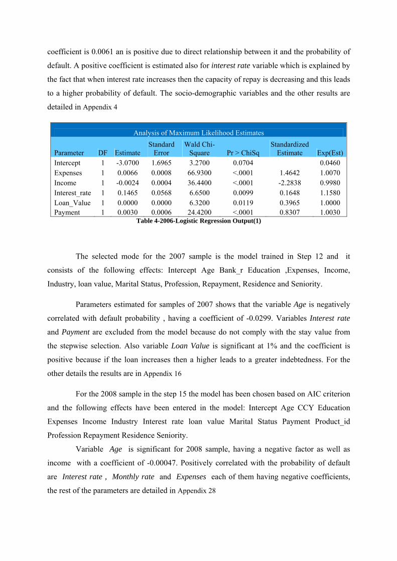
coefficient is 0.0061 an is positive due to direct relationship between it and the probability of

default. A positive coefficient is estimated also for interest rate variable which is explained by

the fact that when interest rate increases then the capacity of repay is decreasing and this leads

to a higher probability of default. The socio-demographic variables and the other results are

detailed in Appendix 4

Analysis of Maximum Likelihood Estimates

Parameter DF Estimate Standard

Error Wald Chi-

Square Pr > ChiSq Standardized

Estimate Exp(Est)Intercept 1 -3.0700 1.6965 3.2700 0.0704 0.0460 Expenses 1 0.0066 0.0008 66.9300 <.0001 1.4642 1.0070 Income 1 -0.0024 0.0004 36.4400 <.0001 -2.2838 0.9980 Interest_rate 1 0.1465 0.0568 6.6500 0.0099 0.1648 1.1580 Loan_Value 1 0.0000 0.0000 6.3200 0.0119 0.3965 1.0000 Payment 1 0.0030 0.0006 24.4200 <.0001 0.8307 1.0030

Table 4-2006-Logistic Regression Output(1)

The selected mode for the 2007 sample is the model trained in Step 12 and it

consists of the following effects: Intercept Age Bank_r Education ,Expenses, Income,

Industry, loan value, Marital Status, Profession, Repayment, Residence and Seniority.

Parameters estimated for samples of 2007 shows that the variable Age is negatively

correlated with default probability , having a coefficient of -0.0299. Variables Interest rate

and Payment are excluded from the model because do not comply with the stay value from

the stepwise selection. Also variable Loan Value is significant at 1% and the coefficient is

positive because if the loan increases then a higher leads to a greater indebtedness. For the

other details the results are in Appendix 16

For the 2008 sample in the step 15 the model has been chosen based on AIC criterion

and the following effects have been entered in the model: Intercept Age CCY Education

Expenses Income Industry Interest rate loan value Marital Status Payment Product_id

Profession Repayment Residence Seniority.

Variable Age is significant for 2008 sample, having a negative factor as well as

income with a coefficient of -0.00047. Positively correlated with the probability of default

are Interest rate , Monthly rate and Expenses each of them having negative coefficients,

the rest of the parameters are detailed in Appendix 28

Logistic Regression –2nd Method 

For 2006 sample according to Information Value criterion variables introduced in the

model are: EDUCATION,EXPENSES,INCOME, NDUSTRY,INTEREST_RATE,LOAN_VALUE_RON,

MARITAL_STATUS,PAYMENT_RON,PRODUCT_ID,PROFESSION,REPAYMENT,RESIDENCE,TERM

and SENIORITY.

The null hypothesis of the Likelihood Ratio test37 is rejected this meaning that none

of the parameters are equal to zero.

Analysis of Maximum Likelihood Estimates Parameter DF Estimate Standard Wald Pr > ChiSq Standardized Exp(Est) Error Chi-Square Estimate Intercept 1 -8.5738 2.1930 15.2900 <.0001 0.0000 Age 1 -0.0240 0.0190 1.5800 0.2082 -0.1210 0.9760 Expenses 1 0.0062 0.0008 60.6900 <.0001 1.3770 1.0060 Income 1 -0.0022 0.0004 31.0400 <.0001 -2.1109 0.9980 Interest_rate 1 0.3224 0.0911 12.5400 0.0004 0.3629 1.3810 Loan_Value 1 0.0000 0.0000 0.1200 0.7344 -0.0986 1.0000 Payment 1 0.0039 0.0010 13.6700 0.0002 1.0640 1.0040 Term 1 0.0001 0.0001 1.6300 0.2011 0.1649 1.0000

Table 5-2006-Logistic Regression Output(2)

For the second method of variable selection variables Term, Age and Loan Value did

not meet the conditions of being significant ,not even at 10% confidence level. Payment

,Interest Rate and Expenses have a positive coefficient estimated and this indicates that for

every increase in this variable increases the probability of default of the borrower(Table 2)

For 2007 Sample considering the Information Value Criterion (Table 2) I introduced

in the model the variables with IV larger than 0.1 and the results obtained indicates that for

instance, comparing with 2006, variable Age is significant and negative correlated with the

default probability of a client considering the fact that if a person is getting old then its

income should increase and be more responsible and the results are shown in his capacity of

repayment of the credit. In the same manner as for the 2006 sample the variables regarding his

capacity of repayment are significant (Expenses, Income ,and Payment).What is very

interesting is that variable Loan Value is also not significant but the Interest Rate variable is

only at 5% level of confidence(Appendix 18-2007-Logistic Regression Output(2)Appendix 18)

                                                            37 More details are shown in Annex: 

After applying the Information Value criterion(Table 2) the results for 2008 sample

indicates that variable Term is indicative for finding the probability of default and related

coefficient of -0.00009 explained by the fact that increasing of term the monthly repayment

decreases and its ability to pay increases. Also long term loans are mortgages that have a

lower risk compared to the consumer due to collateralized process(Appendix 30)

Probit Regression‐First Method 

The selected model for 2006 sample, based on the CHOOSE=AIC criterion, is the model

trained in Step 12 and it consists of the following effects:Intercept, Age, Education, Expenses,

Income, Industry .Interest_rate, Marital_Status, Payment_ron, Profession,

Repayment,Residence,Term.

Compared with logistic regression variable Term is significant at a confidence level of 5%.

Probability of default of the customer is directly proportional with the variables: Expenses,

Interest Rate and Payment and negative correlated to Income (Appendix 9)

For 2007 sample the results obtained indicate that Loan Value is significant at 10%

confidence level and the negative coefficient evidence the fact that the higher value of the

loan is specific to mortgage loans and due to lower interest rates on long term decreases the

probability of default also the p-value of 0.0185 for the term coefficient point out he

significance at 5% level of the variable Term.

Analysis of Maximum Likelihood Estimates Parameter DF Estimate Standard Wald Pr > ChiSq Standardized Error Chi-Square Estimate Intercept 1 -4.2889 21.0212 0.0400 0.8383 Age 1 -0.0159 0.0039 16.7800 <.0001 -0.1397 Expenses 1 0.0009 0.0001 284.8100 <.0001 0.6396 Income 1 -0.0004 0.0000 193.1500 <.0001 -1.1973 Interest_rate 1 0.1643 0.0420 15.3200 <.0001 0.3042 Loan Value 1 -0.0000 0.0000 3.6100 0.0573 -0.1398 Payment 1 0.0008 0.0001 53.9200 <.0001 0.5929 Term 1 0.0000 0.0000 5.5500 0.0185 0.1113

Table 6-2007-Probit Regression Estimates(1)

Interest Rate with a estimated coefficient of 0.1963 is significant at 1% confidence level the

same as Income ,Expenses and Loan Value for 2008 sample, and at 5 % confidence level are

significant Age and Payment (Appendix ).The stepwise selection in comparison with 2007

sample excluded from the model the variable Term ,for the rest of the variables that entered in

the model more details are presented in Appendix 33

Probit regression 2nd Method

According to Information Value criterion the variables introduced in the model are the same

used for Logistic Regression for the 2006 sample. The results indicates that the variable Loan

Value is not significant for the model and also Term variable is only at 10% confidence level

significant. In the same frame the output explains the economic relation between Income and

Expenses and the probability that the client defaults Appendix 11

Analysis of Maximum Likelihood Estimates

Parameter DF EstimateStandard

Error

Wald Chi-

Square Pr >

ChiSq Standardized

Estimate Intercept 1 -1.3171 0.4531 8.4500 0.0037 Age 1 -0.0155 0.0038 16.7100 <.0001 -0.1357 Expenses 1 0.0009 0.0001 281.2100 <.0001 0.6277 Income 1 -0.0005 0.0000 202.7600 <.0001 -1.2179 Interest_rate 1 0.0421 0.0224 3.5200 0.0607 0.0780 Loan Value 1 0.0000 0.0000 0.0100 0.9248 -0.0118 Payment 1 0.0006 0.0002 14.0200 0.0002 0.4743 Term 1 0.0000 0.0000 1.4300 0.2312 0.0608

Table 7-2007-Probit Regression Estimates(2)

 

In the 2007 sample model the variables were the same as for the 2006 with the

xception of Profession variable. The results indicates that neither Term or Loan Value are

significant at all and for Interest Rate the confidence level is 10%-Table 7

The fact that the Information Value for the variable Term is increasing in 2008 in

comparison with 2007 it is revealed also by the significance at 5% confidence level the

opposite process happened with the Payment variable that the decreasing of Information

Value makes the level of confidence to be 5% in 2008 versus 2007.

Neural Networks  

West(2000) in his paper made a comparison between neural networks and other techniques

and as an activation function he uses hyperbolic tangent .Bart(2002) recommends using the

logistic function as the activation function.

In order to see the difference between them I compared the results and although the

Misclassification Rate, for the first activation function, is 0.0209 for test sample the error

increases at 0.04 the number of wrong classified clients is 20.Logistic function used in the

second architecture improves the efficiency of the model considering the value of information

criterion AIC. Regarding test sample misclassification error is smaller than the first model

and the number of wrong classified customers is decreasing with 3.For the 2007 sample the

results of AIC and BIC pointed out the neural network using logistic function as fitting better

the data. From the error of misclassification point of view both validation and test error are

smaller for this architecture and the number of wrong classified is decreasing with 5 on the

test sample.

As it can be observed in Table 8 the informational criterion AIC and BIC indicate that the

model that fits better is the one with the logistic type as the activation function. Although the

number of wrong classification is greater in case of this architecture the Average Error

Function is lower and for Validation Sample the Misclassification Rate is lower for this model

than for the one with the activation function with hyperbolic tangent.

Neural Networks Tanh Logistic Train: Akaike's Information Criterion 4121.68000 3953.43000Train: Schwarz's Bayesian Criterion 4992.89000 4824.64000Train: Average Error Function 0.19598 0.18748Train: Error Function 3879.68000 3711.43000Train: Misclassification Rate 0.07234 0.07254Train: Number of Wrong Classifications 716.00000 718.00000Valid: Average Error Function 0.21115 0.20798Valid: Error Function 1194.24000 1176.34000Valid: Mean Squared Error 0.05944 0.05800Valid: Misclassification Rate 0.07284 0.07178Valid: Number of Wrong Classifications 206 203Test: Average Error Function 0.20589 0.19242Test: Error Function 582.25500 544.16500Test: Mean of Squared Error 0.05774 0.05252Test: Misclassification Rate 0.07497 0.07143Test: Number of Wrong Classifications 106 101

Table 8-2007-Neural Networks Results

Goodness of Fit 

In order to evaluate these models I have performed tests that lead to a model that maps the

best outcomes from actual data. Considering that the sample is split tests were performed on

all three samples but the final decision was taken based on the test results.

Results "in -sample" are the one from the training part, where the parameters were estimated

,and AUROC test ,for 2006,indicates that the neural network model is closest to the perfect

model. In terms of prediction error (Brier score) all same type of model is the better one.

Considering that one of the main reasons for achieving these models is the detection of the

defaulters, this rate have the highest value for the model that uses neural networks with

logistic activation function type.(Appendix 13)

The results of the test sample shows that the model discriminates best non-defaulters from

defaulters customers, through the KS test, is the model of neural networks with logistic

activation function. Regarding the Brier Score, minimum error is for the same model but

which the stepwise selection logistic regression error is smaller (0.0334) than for neural

network having as activation function the hyperbolic tangent.

 

Figure 4-ROC Curve 2008 Sample

In the graph above are plotted ROC Curves for the six models analyzed for 2008 Test Sample

and as it can be observed and sustained by ,AUROC indicator, the second architecture of

neural network is the mist suitable for this data.

Gini coefficient, or Accuracy Ratio has a value of 0.858 on test data from 2007 for the

logistics function neural network, this model all the other validation criteria. What differs

from 2006 is that the detection of bad customers in the stepwise probit regression is better

than on any type of logistic regression.

For the test sample from the 2008 indicators pointed out that the model that uses a neural

network with the logistic function is better than the rest of the models in terms of defaulters

detection, discrimination between them and non-defaulters (KS = 0.6499) and in what

concerns the prediction error on each client, Brier Score, achieve minimum to this model

(0.0754).

To be noted that the defaulters detection accuracy is 0.5952 when logistic regression with the

selection criterion variables Information Value is used and this value is equal to the neural

network model using hyperbolic tangential function.

Out of sample and out‐of time estimation. 

To validate a model it must meet certain minimum conditions in terms of error on the test

samples (out of sample) and the scale of time. Most variables, the socio-demographic changes

during the one year (the period of estimated probabilities of default) but this change is a

slower than that in case of financial variables (income, expenses).

In order to observe this error on test sample out of time of the model estimated I apply the

best model from 2006 sample on 2007 test data and the best model from 2007 I tested on

2008 data .Like I presented in the Goodness of Fit Test Section for the each sample in part

the model that has the most accurate results is the Neural Network using logistic function for

activating the nodes.

0.5 Confusion Matrix Goodness of Fit

Model Sample TN FN TP FP Sensitivity Specificity Misclass

Rate KS AUROC AR

Brier Score

NN2_2008

test 1199 95 157 50 0.6230 0.9600 0.0966 0.6499 0.9104 0.8208 0.0754

NN2_07_08

test 1230 162 90 19 0.3571 0.9848 0.1206 0.5679 0.8550 0.7100 0.0978

NN2_2007

test 1203 74 110 27 0.5978 0.9780 0.0714 0.7415 0.9290 0.8580 0.0525

NN2_06_07

test 1180 134 50 50 0.2717 0.9593 0.1301 0.4618 0.7945 0.5891 0.1096

Table 9-Out of time /sample Results

As it can be observed in Table 9,Area under the Curve, for the out-of time estimation for 2007

is 0.7945 and considering that the same indicator for 2006 sample for test data was 0.9491

and the misclassification rate is 13%.

For the other out-of time analysis applied on 2008 data the results are more closely ,for

instance Accuracy Ratio is 0.71 and for 2008 data the value is 0.8208 .Considering the fact

that applying the same model in the same period 2007 the area under the curve is improving

with only 9% relative difference .

This approach is a recommendation from the Basel II Validation Guide and the fact that a

model applied on a different test data on a different scale of time it only sustains its robustness

and the fact that the models accuracy are higher is not only due to data variables and

connection and also its model itself.

4.2 Portfolio analysis.  

In the second logistic regression variable portfolio Interest Rate is not significant but in this

included in the Term variable model and has a coefficient (-0.0006) p-value less than 0001,

explaining the relationship between long-term loans, generally mortgages and default

probability. Variable loan value is significant in both logistic regression and 5% Income and

Expenses variables have coefficients very close as values for the two models.

For the probit regression the results indicated also that Interest Rate for the second regression,

the one with variable selection based on Information Value ,is not significant at any level and

also the variable term is included in the model. For the stepwise probit regression all financial

variables are significant at 1% confidence level(Appendix 46)

Neural Networks Tanh Logistic Train: Akaike's Information Criterion 10510.42000 10046.78000 Train: Schwarz's Bayesian Criterion 11678.73000 11215.09000 Train: Average Error Function 0.21909 0.20915 Train: Error Function 10220.42000 9756.78000 Train: Misclassification Rate 0.07893 0.07631 Train: Number of Wrong Classifications 1841 1780 Valid: Average Error Function 0.22910 0.22547 Valid: Error Function 3053.48000 3005.10000 Valid: Mean Squared Error 0.06530 0.06478

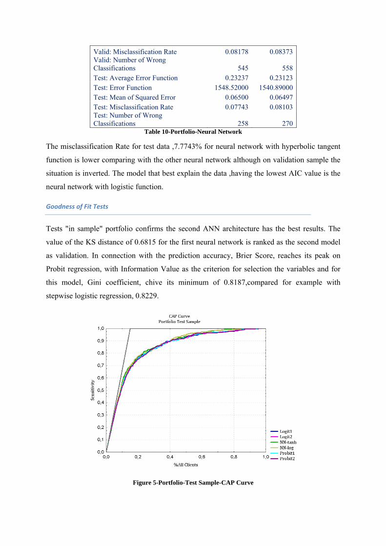
Valid: Misclassification Rate 0.08178 0.08373 Valid: Number of Wrong Classifications 545 558 Test: Average Error Function 0.23237 0.23123 Test: Error Function 1548.52000 1540.89000 Test: Mean of Squared Error 0.06500 0.06497 Test: Misclassification Rate 0.07743 0.08103 Test: Number of Wrong Classifications 258 270

Table 10-Portfolio-Neural Network

The misclassification Rate for test data ,7.7743% for neural network with hyperbolic tangent

function is lower comparing with the other neural network although on validation sample the

situation is inverted. The model that best explain the data ,having the lowest AIC value is the

neural network with logistic function.

Goodness of Fit Tests 

Tests "in sample" portfolio confirms the second ANN architecture has the best results. The

value of the KS distance of 0.6815 for the first neural network is ranked as the second model

as validation. In connection with the prediction accuracy, Brier Score, reaches its peak on

Probit regression, with Information Value as the criterion for selection the variables and for

this model, Gini coefficient, chive its minimum of 0.8187,compared for example with

stepwise logistic regression, 0.8229.

 

Figure 5-Portfolio-Test Sample-CAP Curve 

 

The fact that the results of the out-of samples indicate the same pattern as at best, can only

confirm the consistency of analysis. However in this case, detection accuracy of the

defaulters is higher for neural network model with the hyperbolic tangent function, which is

confirmed by results presented above, when I mentioned the increasing number of wrong

classified customers if it is using the logistics function for neural network.

Cumulative Accuracy Profile graph for wich i have calculated the area under this curve ,this

being the Accuracy Ratio points aut that the two curves og=f the that neural networks are well

above the curves of the other models, especially over probit regression who has the smallest

value of this indicator 0.8061 compared with the second neural network, 0.8314 and

compared to the perfect model that reaches the value of 1. 

4.3 Portfolio with macroeconomic variable.  

The implementation of this macroeconomic variable is made on the same samples of portfolio

and the model is estimated on training sample with regarding of validation test on the test

sample.

Analysis of Maximum Likelihood Estimates

Parameter DF Estimate Standard Error Wald Chi-

Square Pr >

ChiSq Standardized

Estimate Intercept 1 -3.6365 1.4412 6.3700 0.0116 Age 1 -0.0184 0.0044 17.8900 <.0001 -0.0914 Expenses 1 0.0018 0.0001 552.9500 <.0001 0.6611 Income 1 -0.0007 0.0000 387.6800 <.0001 -1.3555 Interest_rate 1 0.1146 0.0279 16.8800 <.0001 0.1417 Loan Value 1 0.0000 0.0000 27.7500 <.0001 -0.3528 Payment 1 0.0023 0.0001 250.6900 <.0001 1.2525 IMV_customer 1 5.1807 0.3196 262.7200 <.0001 0.2641

Table 11-Portfolio Macro Stepwise Logistic Regression

The model with macroeconomic variable included leads to an improvement of the

significance of some variables such as loan value and Interest Rate. Also another deduction is

that Income and Expenses have smaller values of coefficients in this model a part of their

importance being transfer to the new variable IMV_customer also significant at 1%

confidence level. For the stepwise probit regression the financial variables are all significant

at 1% and in both models the Term variable is not selected to be part of the estimation.

Neural Networks Tanh Logistic

Train: Akaike's Information Criterion 9381.67000 9337.05000 Train: Schwarz's Bayesian Criterion 10574.14000 10529.53000 Train: Average Error Function 0.19476 0.19381 Train: Error Function 9085.67000 9041.05000 Train: Misclassification Rate 0.07374 0.07117 Train: Number of Wrong Classifications 1720.00000 1660.00000 Valid: Average Error Function 0.21533 0.21072 Valid: Error Function 2869.89000 2808.47000 Valid: Mean Squared Error 0.06174 0.06047 Valid: Misclassification Rate 0.08013 0.07773 Valid: Number of Wrong Classifications 534 518 Test: Average Error Function 0.21861 0.20920 Test: Error Function 1456.78000 1394.12000 Test: Mean of Squared Error 0.06138 0.05939 Test: Misclassification Rate 0.07713 0.07593 Test: Number of Wrong Classifications 257 253

Table 12-Portfolio Macro -Neural Network

Difference in the number of training cases wrong classified is 60 in favour of neural network

that uses logistic function as activation function and also for the validation sample the

detection error is smaller for this model. Among 3332 of clients 253 were wrong classified on

test sample for the model mentioned above and considering the fact that for the portfolio

analysis the situation was reversed and for the first method the number was 258 and the for

the second method the same number was 270 ,it can be observed the major improvement

brought by the macroeconomic variable.

Goodness of Fit Tests: 

Testing "out of sample" results for portfolio with macroeconomic variables incorporated

maintain the idea of the performance for neural networks models over the rest models. In this

manner to see the improved results for these models compared with the portfolio, I made an

analysis showing relative changes of each indicator in order to move from the global analysis

of the overall portfolio, with and without this new variable, to each indicator and the

improvement in every technique I used for modelling.(Appendix 63)

                             

Figure 6-Comparison between Neural Networks models

Detection accuracy of defaulters customers increases on average with 5.85% for probit

regressions and with 3% for logistic regressions, neural networks instead recorded an

increase of only 1.13%. Regarding the prediction error for each customer, on average

decreases 4% for the two types of regression and the improvement gave by the neural

networks is 7.5% .Accuracy Ratio improves with 1.73% for the neural network with

hyperbolic tangent function while logistic regressions bring increase in average equal to 1%.

                

Figure 7-Comparison among logistic regression and Neural Networks

As it can be seen in the graph above the regression logistic with macroeconomic variable

incorporated is comparable with neural networks and on some fractions the report between 1-

error type 1(hit rate) and error type II (false alarm rate) is greater than for the neural networks

using hyperbolic tangent function.

The Spiegelhalter Test indicates that, by accepting the null hypothesis on both portfolios with

and without the macroeconomic variable, the observed default rates are close to the estimated

probabilities of default(Appendix 68)

Dynamic Cut off portfolio with macroeconomic variables 

When using the cut-off or 0.5 in order to classify customers a disequilibrium could increase

costs for defaulter detection. To solve this problem a new cut-off should be used and in order

to find the theoretical cut-off the intersection of the corrected rate for discriminating the non

defaulters and defaulters is offering the desired result. When this process is made the

differences between Sensitivity and Specificity should be zero because their point of

intersection is the new value of the cut-off.

 

Figure 8-Portfolio Macro Cut-Off Dynamic

The results of the portfolio with macroeconomic variable incorporated are recalculated with

the new values of cut-off. The value of cut-off is determined on the training sample and

applied then on the default probabilities obtained from the modes described in this paper.

Although the optimal threshold is then applied on the test sample and this could affect the

performance of the models but the predictions made on test samples are completely

independent on the training samples which will be also seen as in practice where credit

decision and management is involved in setting this cut-off. Many factors are involved when

setting this threshold but the one that affect the portfolio of a bank is the fact that a lower

value of this cut off will be translated as an acceptance rate higher which it turn into

profitability for the bank if the clients accepted wouldn’t default in a larger proportion.

This issue of acceptance rate is a trade-off between the higher acceptance rate as profit

generator and lower acceptance rate as loss in market share is well weighted in a bank

strategic decisions .The results on test sample indicates the fact that for the new cut-off the

detection of defaulter clients has been increased while the detection on non-defaulter clients

has been decreased. Even if on training sample the difference between those two is on average

equal to 0.001 the same average on the test results is -0.0079 meaning that using the cut-off

from training sample to test sample isn’t a mismeasurement. 

4.3 Misclassification Cost  

The model that minimizes the expected future loss is an optimal model of classification and

considering the fact that there are two classes of customers the future loss depends on the two

types of misclassification errors.

Where and are the population percentage of defaulters and non-defaulters clients and

is the cost of error type I respectively cost of error type II. The choice of these two

costs has a major impact on the evaluation of the model and the factor that affect the costs are

difficult to be quantified. The Error of Type I is the cost of granting a loan to a customer that

is defaulter and the Error of Type II is the opportunity profit of rejecting a non-defaulter client

considered as bad. In this way for the first type of error the costs are related to loss of

principal money and other costs that interfere in the process of recovery. For the type II error

the lost of interest paid by de client and the profit obtained from his loan is the virtual earn

missed by the bank.

Having clarified this idea is understandable that potential loss is more expensive than lost

profit, in this way cost values should be differentiate. In this paper I took into consideration a

proportion of the cost of 5.10 and 15 this being the multiplier for Type I error compared with

type II error.These selected values for cost are sustained by bank policy whose portfolio I

used in this research,and this was calculated by incorportaing the cost of risk.

The main idea of this analysis is to see the impact of misclassification cost on the

results of the models analyzed. First I explored the results with cost of 5 and by comparison

with the initials models for portfolio ,without macroeconomic variable ,on test sample ,the

defaulter accuracy ratio has improved most on Probit Regression with Information Value and

on the second place is the logistic regression with the same selection type of variables. Even

the first type of probit and logistic regression recorded a higher increase on this indicator than

other neural network model.Cost of 10 improves probit regression and reduce the error of

prediction with 3.3% and neural networks on the same indicator has been improved with

6.8%.

The same thing happened when a cost of 15 has been used ,but the improvement of

the stepwise logistic regression on misclassification error ratio is 5.31% and for neural

network is 5.55 % but if the latter value is the highest for neural network ,for regressions the

higher improvement is recorded on the second type of probit regression with a 8.44% relative

modification.  

After all three types of scores gave been incorporated into the model analyzed I

compared them through Kuipers Score and Granger-Pesaran Test.As it can be noticed the

hypothesis null of classification failure could be rejected at one-percent level of significance

for all model for all three types of costs. Kuipers Score is the difference between hit rate and

false alarm rate and the grater the difference the better the classification between defaulters

and non-defaulters is made. The models that have la higher score are neural networks and

from regressions class the stepwise logistic is the one that discriminate better. 

4.4 Stress Testing  

For credit risk modeling the stress testing is based not only on scenario tests but on sensitivity

tests and according to Basel II the objective is not to require banks to consider worst-case

scenarios but to capture the different behaviors and mixtures of simulations in order to create

a real scenario possibility. Studies on credit risk stress testing come with three or four

scenarios ,one is the baseline and the other are related to decreasing of GDP ,a rise of real

interest rate and a reduction in real property prices by different values. 

 

 

 

 

Considering the related to the loan agreement signed with the IMF the reduction plan

is to cutt wages with the following percentages 25% and those Cuts will come into effect

starting June 1st.

The scenario that I considered it is based on stressing the income of customers having

„Public Service” as industry .The assumptions are that the their income are decreasing with

25% and for the rest of the portfolio this variables remain the same. Regarding expenses I

proposed to capture a raise in inflation, that will be translated to an increase in the level of

expenses and considering that the target inflation is 3.5% plus 1% error band I stressed the

values of the variable Expenses with an increase with 4.5%

After recalculating the probabilities of default the results concluded that this scenario

impact the losses with an increase of 0.25% on the entire portfolio and only on the public

employers the impact is 1% on the average probability of default on both models (stepwise

logistic regression and logistic neural networks).On the graph below it can be observed the

differences between the estimated probability of default on original data and on stressed data ,

on the selected portfolio public employers, on test sample .

 

 

Figure 9-Portfolio Macro Stress Testing

 

 

 

 

 

 

5.Conclusions  

In this paper I have highlighted both the comparison of several models of credit

scoring and improvement necessities that have to be done for such models. The initial idea I

had was a transposition of several models on both scale of time and on the unit, meaning

model estimation and data analysis from different years and on different customers. The

conclusion of applying these models on different years was that, certain financial variables,

like Income or Expenses are significant regardless of the chosen time axis. What is important

to emphasize here is that although socio-demographic variables, during one year, tend to have

a rate of change smaller than for financial variables and there exist some connections such as

variable Seniority, age of work at previous job, was included in almost all models and the

explanation being that this variable is the bridge between financial and non-financial

variables. If the seniority is higher then there are two options, have an adequately income and

wants stability, or there is a higher probability that in the next period will want to change their

workplace but automatically income will be raised or remains the same which is negatively

correlated with probability of default given. This analysis captures both the evolution of the

three periods of varying models importance and their importance in itself and an important

aspect is that usually a multi-year analysis incorporates behavioral variables that are meant to

hold a more correct image of the client's position just like a compass, so the bank will be able

to act in time. Finding that the results on the test samples for out-of sample and out-of-time

are quite robust I grouped data at a level of portfolio in order to capture the relationships with

the economic environment of the period between 2007 and 2009 in Romania.

Portfolio results supported findings from different years, so that neural networks have

a higher accuracy than the regressions. In order to surprise the whole picture and the

framework of the portfolio I analyzed in this paper, I proposed a new approach of

determining the level of customer macroeconomic impacts. So going from one macro

vulnerability indicator proposed in the literature by Herrera and Garcia I calculated an

indicator that its designation is to capture the capacity of repayment of a customer and to also

to see its future problems with this issue. First I made this indicator at global level on monthly

data and the impact will be performed by reporting this to its degree of indebtedness and the

spread for the interest rate that has taken credit.

This indicator of macroeconomic vulnerability could be part of a development model

for credit risk based on a scorecard where the capacity of a client would be aligned to the

period he is taking the loan because if the period is under pressure a small deviation of his

behavior will be amplified by the macroeconomic conditions and he will be overdue with his

monthly payments and in the end classified as default client.

What is interesting is that once I re-estimated the parameters , results showed that

models like logistic regressions have accuracy as high as one of the neural network

architectures. To study the impact of each model I computed an improvement ratio to detect

which technique is getting improved related to the inclusion of this new variable because

some models had high accuracy before, like neural networks. Considering the detection

accuracy of default clients the regressions techniques have a much greater improvement than

any other model. This detection is very important for bad customers due to their

expensiveness in comparison with the non-detection of good clients and in order to explore

this area I included in the models a loss function depending on the two types of costs. I

analyzed three types of proportions between those costs and the results indicated that cost

improvements of a logistic regression or probit type are comparable or even higher than an

improvement of the neural networks.

All analysis have been sustained by the minimal error of detection between default

realized rate and default predicted rate and by statistics test that confirmed that models have

no major differences between distributions of the two probabilities of default.

What I wanted to evidence in this paper is that more important than a particular model

is the variable selection and choice of loss function that need to be minimized in order to treat

the tradeoff between the profit considerations and best classification of customers.

For the further research I would like to incorporate both behavioral and

macroeconomic variable in a survival analysis to detect not only if the customer defaults but

when this event happens in order to help a bank to have enough capital when a part of the

portfolio is translated from a rating class to other and you don’t know when this migration

ends because in the end you know it will be a default client.

6.References  

Andersen, H(2008),"Failure prediction of Norwegian banks: A logit approach" ,

Financial Market Department, Norges Bank. 

Baesens,B. (2003), “Developing intelligent systems for credit scoring using machine

learning techniques” Ph.D. thesis, K.U.Leuven

Balcaen, S. and H. Ooghe, (2004). Alternative methodologies in studies on business

failure: do they produce better results than the classical statistical methods? Working

Paper 2004/249, Faculteit Economie en Bedrijfskunde

Balzarotti V, M. Gutiérrez and G.V. Vallés (2006),"Credit Scoring models with

truncated samples and their validation "NationalBank of Argentina

Banasik, J,J.N. Crook, and L.C. Thomas.(1999),”Not if but when will borrowers

default” Journal of the Operational Research Society

Banasik, J.N. Crook, and L.C. Thomas (2001),” Sample selection bias in credit scoring

models” In Proceedings of the Seventh Conference on Credit Scoring and Credit

Control (CSCCVII'2001), Edinburgh, Scotland

Banasik, J., Crook, J., Thomas, L. (2003), "Sample selection bias in credit scoring

models", Journal of the Operational Research Society, Vol. 54 No.8

Biancotti C, L. D’Aurizio and R. Polcini (2007),"A neural network architecture for data

editing in the Bank of Italy’s business surveys" National Bank of Italy

Bishop, C. (1995), “Neural Networks for Pattern Recognition”, Clarendon Press,

Oxford

BCBS, Basel Committee on Banking Supervision, 1988. International Convergence of

Capital Measurement and Capital Standards. Bank for International Settlements,July

1988

BCBS, Basel Committee on Banking Supervision, 2003. Press releas: Significant

Progress on Major Issues . Bank for International Settlements, 11 October 2004

BCBS, Basel Committee on Banking Supervision, 2004. International Convergence of

Capital Measurement and Capital Standards. A Revised Framework. Bank for

International Settlements, June 2004

BCBS, Basel Committee on Banking Supervision, 2005. Studies on the Validation of

Internal Rating Systems. Working paper no. 14, Basel Committee on Banking

Supervision, February 2005

Crook,J John Banasik,(2004)," Does reject inference really improve the performance of

application scoring models? "Journal of Banking & Finance

Engelmann B and R Rauhmeier(2006),"The Basel II Risk Parameters",Springer

Härdle W,2007,"Estimating probabilities of default with support vector machines ",

Deutsche Bank

Kočenda E, Martin Vojtek (2009), “Default Predictors and Credit Scoring Models for

Retail Banking”, Working paper, Prague

Komorád K.(2002), “On Credit Scoring Estimation” Master’s Thesis, Institute for

Statistics and Econometrics, Humboldt University, Berlin

Ming-Chun Tsai, Shu-Ping Lin, Ching-Chan Cheng, Yen-Ping Lin (2009), “The

consumer loan default predicting model – An application of DEA–DA and neural

network”, Expert Systems with Applications 36

Oestereichische Nationalbank, 2004. Guidelines on Credit Risk Management, Rating Models

and Validation

Rommer, A. D., 2005b. Testing the Assumptions of Credit-scoring Models. WP no.28,

Danmarks NationalbankŘezáč,M,F. Řezáč and Masaryk(2008),"Measuring the Quality of

Credit Scoring Models", University, Czech Republic

Roszbach(2003)," Bank Lending Policy,Credit Scoring and the Survival of Loans" ,

SVERIGES RIKSBANK

Silva da R.,,A.C.Magalhães da Silva(2009)-" The Influence of Collateral on Capital

Requirements in the Brazilian Financial System: an approach through historical average and

logistic regression on probability of default",National Bank of Brazilia

Siddiqi N(2006),"Credit Risk Scorecards Developing and Implementing Intelligent Credit

Scoring"

Thomas, D.B. Edelman si J.N. Crook (2002), „Credit Scoring and Its Applications”,SIAM

West,D.(2000),” Neural network credit scoring models”. Computers and Operations Research

 

7.APPENDIX

Variable Characteristics No. %

Credit_nr Unique no. 33,321 Repayment so far no credit customer 24,001 72.03%

Yes (In some cases warnings required) 1,556 4.67% Yes (never warned or deferred) 7,764 23.30%

Sex Female 9,955 29.88% Male 23,366 70.12%

Age Continuous variable Marital_Status Divorce 1,111 3.33%

Married 23,118 69.38% Single 8,787 26.37% Widowed 305 0.92%

Education High School 12,536 37.62% Primary school 451 1.35% University 20,334 61.02%

Profession Employee 31,031 93.13% Own Empl 1,259 3.78% Unemploy 511 1.53% Worker 520 1.56%

Seniority < 6 Months 2,116 6.35% > 10 Years 9,570 28.72% 0,5 - 1 Year 3,437 10.31% 1 - 2 Years 6,953 20.87% 3 - 5 Years 5,951 17.86% 6 - 10 Years 5,294 15.89%

Industry Agriculture 121 0.36% Bank and Financial Services 1,990 5.97% Construction 1,068 3.21% Electronics / Pharmaceutical / Optics 700 2.10% Food 259 0.78% Gastronomie 127 0.38% Leather / Textile / Clothing 210 0.63% Other 14,799 44.41% Plastic / rubber / asbestos 71 0.21% Public Service 11,161 33.50% Retail 765 2.30% Steel/metal processing 926 2.78% Stones / earth / gas / ceramic 730 2.19% Wholesale 207 0.62% Wood 187 0.56%

Residence Job apartment 117 0.35% Own house 19,622 58.89%

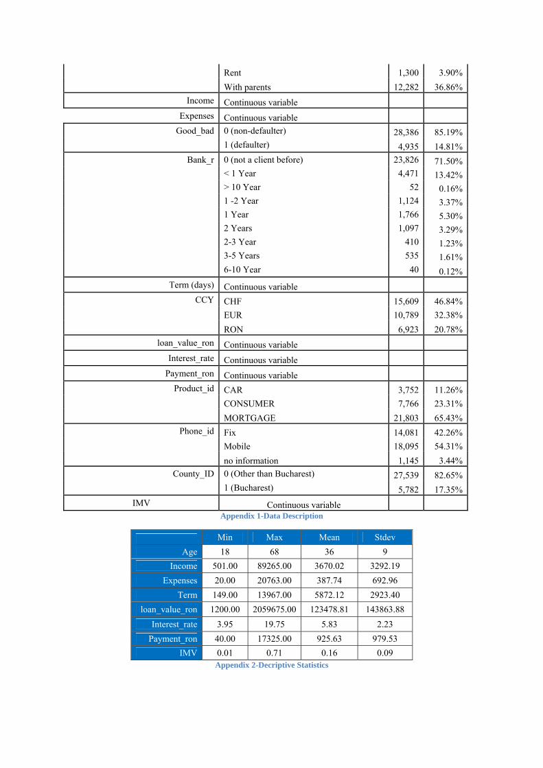
Rent 1,300 3.90% With parents 12,282 36.86%

Income Continuous variable Expenses Continuous variable

Good_bad 0 (non-defaulter) 28,386 85.19% 1 (defaulter) 4,935 14.81%

Bank_r 0 (not a client before) 23,826 71.50% < 1 Year 4,471 13.42% > 10 Year 52 0.16% 1 -2 Year 1,124 3.37% 1 Year 1,766 5.30% 2 Years 1,097 3.29% 2-3 Year 410 1.23% 3-5 Years 535 1.61% 6-10 Year 40 0.12%

Term (days) Continuous variable CCY CHF 15,609 46.84%

EUR 10,789 32.38% RON 6,923 20.78%

loan_value_ron Continuous variable Interest_rate Continuous variable

Payment_ron Continuous variable Product_id CAR 3,752 11.26%

CONSUMER 7,766 23.31% MORTGAGE 21,803 65.43%

Phone_id Fix 14,081 42.26% Mobile 18,095 54.31% no information 1,145 3.44%

County_ID 0 (Other than Bucharest) 27,539 82.65% 1 (Bucharest) 5,782 17.35%

IMV Continuous variable Appendix 1-Data Description

Min Max Mean Stdev Age 18 68 36 9

Income 501.00 89265.00 3670.02 3292.19 Expenses 20.00 20763.00 387.74 692.96

Term 149.00 13967.00 5872.12 2923.40 loan_value_ron 1200.00 2059675.00 123478.81 143863.88

Interest_rate 3.95 19.75 5.83 2.23 Payment_ron 40.00 17325.00 925.63 979.53

IMV 0.01 0.71 0.16 0.09 Appendix 2-Decriptive Statistics

  

 

Appendix 3-2006-Stepwise Seletion Logistic Regression

 

 

Appendix 4-2006-Logistic Regression Output(1) 

 

Appendix 5-2006-LR test Logistic Regression(2)

 

Appendix 6-2006-Logistic Regression Output(2)

 

 

Appendix 7-2006-Stepwise Selection Probit Regression

 

 

Appendix 8-2006-LR test Probit Regression (1)

 

Appendix 9-2006-Probit Regression Output(1)

 

 

 

Appendix 10-2006-LR Test -Probit Regression (2)

 

 

 

Appendix 11-2006-Probit Regression Output(2)

 

 

Appendix 12-2006-Neural Networks Output

 

 

TN FN TP FP Sensitivity Specificity Misclassification Rate

KS AUROC ARBrier Score

Logit1 validation 763 27 33 11 0.5500 0.9858 0.0456 0.8208 0.9422 0.8843 0.0350

Logit1 test 387 17 12 2 0.4138 0.9949 0.0455 0.8261 0.9153 0.8307 0.0334

Logit1 training 2747 77 82 14 0.5157 0.9949 0.0312 0.7990 0.9641 0.9282 0.0252

Logit 2 validation 765 29 31 9 0.5167 0.9884 0.0456 0.8258 0.9438 0.8875 0.0347

Logit 2 test 387 18 11 2 0.3793 0.9949 0.0478 0.8154 0.9156 0.8312 0.0346

Logit 2 training 2747 77 82 14 0.5157 0.9949 0.0312 0.7990 0.9641 0.9282 0.0252

NN1 test 384 15 14 5 0.4828 0.9871 0.0478 0.8297 0.9520 0.9041 0.0342

NN1 training 2749 49 110 12 0.6918 0.9957 0.0209 0.8493 0.9826 0.9651 0.0170

NN1 validation 764 17 43 10 0.7167 0.9871 0.0324 0.8067 0.9669 0.9339 0.0294

NN2 training 2749 40 119 12 0.7484 0.9957 0.0178 0.9114 0.9901 0.9801 0.0147

NN2 validation 767 14 46 7 0.7667 0.9910 0.0252 0.8611 0.9745 0.9491 0.0236

NN2 test 387 15 14 2 0.4828 0.9949 0.0407 0.8209 0.9530 0.9060 0.0315

Probit 1 validation 764 35 25 10 0.4167 0.9871 0.0540 0.8158 0.9414 0.8829 0.0382

Probit 1 test 387 20 9 2 0.3103 0.9949 0.0526 0.7927 0.9136 0.8271 0.0362

Probit 1 training 2747 86 73 14 0.4591 0.9949 0.0342 0.7856 0.9597 0.9194 0.0281

Probit2 validation 766 33 27 8 0.4500 0.9897 0.0492 0.7975 0.9401 0.8803 0.0377

Probit2 test 387 21 8 2 0.2759 0.9949 0.0550 0.7927 0.9105 0.8209 0.0375

Probit2 training 2749 89 70 12 0.4403 0.9957 0.0346 0.7911 0.9608 0.9216 0.0279

Confusion Matrix Goodness of fit TestsTechnique Sample

 

Appendix 13-2006-Goodness of fit results

 

 

Appendix 14-2006-ROC Curve Test Sample

 

   

Appendix 15-2007-Stepwise Selection Logistic Regression

 

 

Appendix 16-2007-Logistic Regression Output(1)

 

Appendix 17-2007-LR Test Logistic Regression(2)

 

Appendix 18-2007-Logistic Regression Output(2)

 

 

 

Appendix 19-2007-Stepwise Selection-Probit Regression

Appendix 20-2007-LR Test-Probit Regression(1)

 

 

 

 

Appendix 21-2007-Probit Regression Output(1)

 

Appendix 22-2007-LR Test Probit Regression (2)

 

Appendix 23-2007-Probit Regression Output (2)

 

Confusion Matrix Goodness of Fit Model Sample

TN FN TP FP Sensitivity Specificity Misclass Rate

KS AUROC AR Brier Score

Logit1 training 8426 670 686 116 0.5059 0.9864 0.0794 0.6897 0.9187 0.8374 0.0611 Logit1 validation 2395 199 200 34 0.5013 0.9860 0.0824 0.6813 0.9071 0.8143 0.0642 Logit1 test 1207 92 92 23 0.5000 0.9813 0.0813 0.7005 0.9110 0.8220 0.0621 Logit 2 training 8420 684 672 122 0.4956 0.9857 0.0814 0.6864 0.9177 0.8354 0.0622 Logit 2 validation 2388 196 203 41 0.5088 0.9831 0.0838 0.6773 0.9066 0.8131 0.0645 Logit 2 test 1205 93 91 25 0.4946 0.9797 0.0835 0.6942 0.9125 0.8249 0.0623 Probit 1 training 8429 704 652 113 0.4808 0.9868 0.0825 0.6881 0.9181 0.8361 0.0625 Probit 1 validation 2394 208 191 35 0.4787 0.9856 0.0859 0.6743 0.9073 0.8146 0.0653 Probit 1 test 1209 90 94 21 0.5109 0.9829 0.0785 0.6875 0.9108 0.8217 0.0621 Probit2 training 8434 739 617 108 0.4550 0.9874 0.0856 0.6794 0.9145 0.8289 0.0643 Probit2 validation 2395 213 186 34 0.4662 0.9860 0.0873 0.6743 0.9073 0.8146 0.0656 Probit2 test 1209 101 83 21 0.4511 0.9829 0.0863 0.6851 0.9090 0.8180 0.0641 NN1 training 8368 542 814 174 0.6003 0.9796 0.0723 0.7146 0.9340 0.8681 0.0564 NN1 validation 2382 159 240 47 0.6015 0.9807 0.0728 0.6975 0.9207 0.8414 0.0594 NN1 test 1201 77 107 29 0.5815 0.9764 0.0750 0.7291 0.9222 0.8443 0.0577 NN2 training 8365 541 815 177 0.6010 0.9793 0.0725 0.7313 0.9404 0.8808 0.0544 NN2 validation 2381 155 244 48 0.6115 0.9802 0.0718 0.6858 0.9228 0.8457 0.0580 NN2 test 1203 74 110 27 0.5978 0.9780 0.0714 0.7415 0.9290 0.8580 0.0525

Appendix 24-2007-Goodness of Fit Results

 

 

 

Appendix 25-2007 ROC Curve and KS Distance

 

 

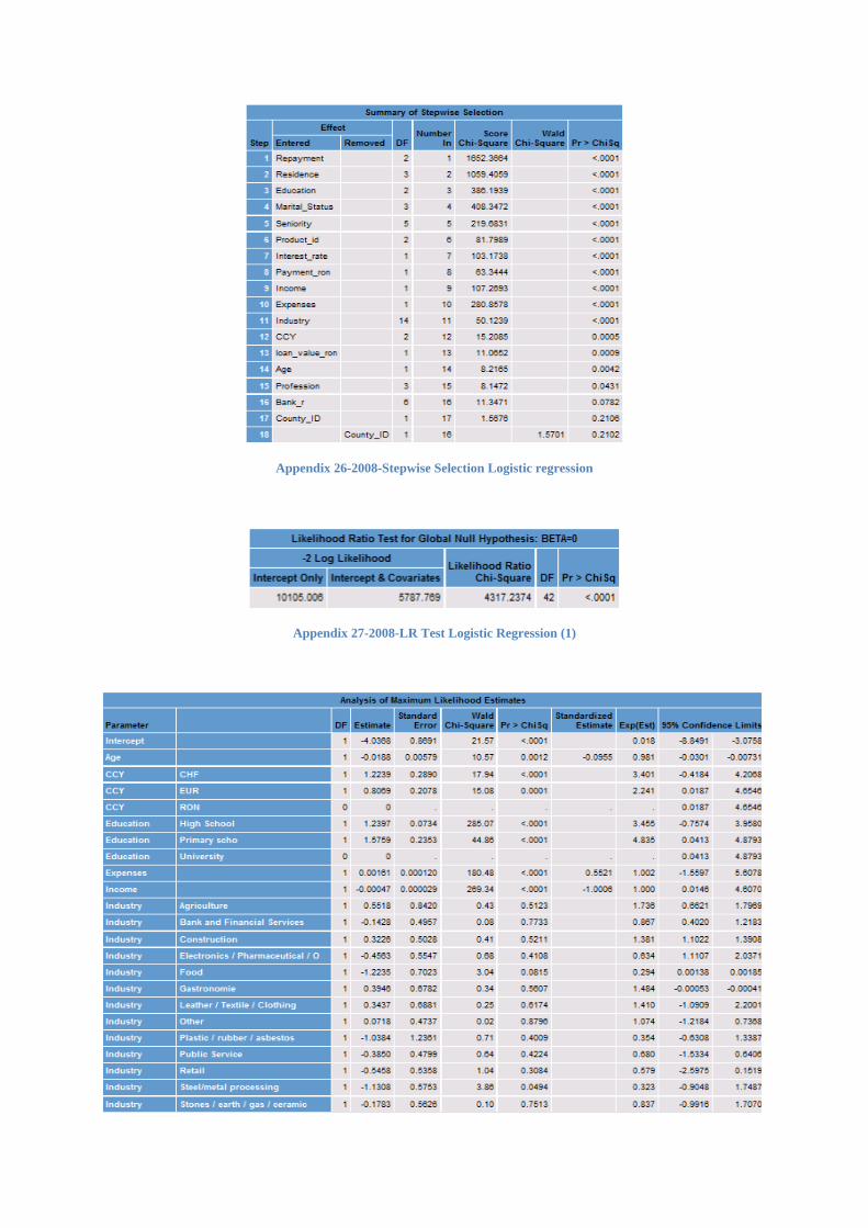
Appendix 26-2008-Stepwise Selection Logistic regression

 

 

Appendix 27-2008-LR Test Logistic Regression (1)

 

 

 

Appendix 28-2008-Logistic Regression Output(1)

 

Appendix 29-2008-LR Test Logistic Regression(2)

 

 

Appendix 30-2008-Logistic Regression Output(2)

 

Appendix 31-2008-Stepwise Probit Regression (1)

Appendix 32-2008-LR Test Probit Regression(1)

 

Appendix 33-2008-Probit Regression Output(1)

Appendix 34-2008-LR Test Probit Regression(2)

 

Appendix 35-2008-Probit Regression Output(2)

 

Neural Networks Tahn Logistic Train: Akaike's Information Criterion 5104.87000 5031.93000 Train: Schwarz's Bayesian Criterion 5983.29000 5910.36000 Train: Average Error Function 0.23143 0.22796 Train: Error Function 4862.87000 4789.93000 Train: Misclassification Rate 0.08576 0.08443 Train: Number of Wrong Classifications 901.00000 887.00000 Valid: Average Error Function 0.24769 0.23676 Valid: Error Function 1487.12000 1421.52000 Valid: Mean Squared Error 0.06901 0.06614 Valid: Misclassification Rate 0.08394 0.07961 Valid: Number of Wrong Classifications 252 239 Test: Average Error Function 0.26263 0.24935 Test: Error Function 788.40600 748.55000 Test: Mean of Squared Error 0.07399 0.07159 Test: Misclassification Rate 0.08861 0.08994 Test: Number of Wrong Classifications 133 135

Appendix 36-2008-Neural Netoworks Results

 

Confusion Matrix Goodness of Fit

Model Sample TN FN TP FP Sensitivity Specificity Misclass

Rate KS AUROC AR Brier Score

Logit1 training 8287 797 1161 261 0.5930 0.9695 0.1007 0.6666 0.9072 0.8143 0.0789 Logit1 validation 2396 228 310 68 0.5762 0.9724 0.0986 0.6537 0.9002 0.8004 0.0787 Logit1 test 1200 104 148 49 0.5873 0.9608 0.1019 0.6480 0.8956 0.7913 0.0785 Logit 2 training 8284 812 1146 264 0.5853 0.9691 0.1024 0.6674 0.9065 0.8130 0.0793 Logit 2 validation 2394 236 302 70 0.5613 0.9716 0.1019 0.6436 0.9000 0.8000 0.0791 Logit 2 test 1196 102 150 53 0.5952 0.9576 0.1033 0.6427 0.8936 0.7872 0.0790 Probit 1 training 8297 856 1102 251 0.5628 0.9706 0.1054 0.6631 0.9050 0.8100 0.0816 Probit 1 validation 2399 243 295 65 0.5483 0.9736 0.1026 0.6351 0.8975 0.7950 0.0814 Probit 1 test 1204 109 143 45 0.5675 0.9640 0.1026 0.6439 0.8961 0.7921 0.0794 Probit2 training 8292 860 1098 256 0.5608 0.9701 0.1062 0.6636 0.9043 0.8086 0.0820 Probit2 validation 2398 246 292 66 0.5428 0.9732 0.1039 0.6314 0.8975 0.7949 0.0816 Probit2 test 1204 109 143 45 0.5675 0.9640 0.1026 0.6316 0.8935 0.7870 0.0798 NN1 training 8349 743 1215 199 0.6205 0.9767 0.0897 0.6891 0.9190 0.8379 0.0714 NN1 validation 2401 207 331 63 0.6152 0.9744 0.0899 0.6757 0.9024 0.8048 0.0741 NN1 test 1212 102 150 37 0.5952 0.9704 0.0926 0.6279 0.8957 0.7914 0.0763 NN2 training 8276 642 1316 272 0.6721 0.9682 0.0870 0.7165 0.9347 0.8694 0.0666 NN2 validation 2374 178 360 90 0.6691 0.9635 0.0893 0.7063 0.9175 0.8350 0.0704 NN2 test 1199 95 157 50 0.6230 0.9600 0.0966 0.6499 0.9104 0.8208 0.0754

Appendix 37-2008-Goodness of Fit Results

 

 

                                 

Appendix 38-2008-KS Distance Test Sample 

 

 

Appendix 39-Portfolio-Stepwise Selection Logistic Regression

Appendix 40-Portfolio-LR Test Logistic Regression(1)

Appendix 41-Portfolio -Logistic Regression Output(1)

 

Appendix 42-Portfolio –LR Test Logistic regression(2)

 

 

Appendix 43-Logistic Regression Output(2) Portfolio

Appendix 44-Portfolio-Stepwise Selection Probit

Appendix 45-Portfolio LR Test Probit Regression(1) 

 

 

Appendix 46-Portfolio-Probit Regression Output(1)

 

Appendix 47-Portfolio-LR Test Probit Regression(2)

Appendix 48-Portfolio-Probit Regression Output(2)

0.5 Confusion Matrix Goodness of Fit

Model Sample TN FN TP FP Sensitivity Specificity Misclass KS AUROC AR Brier Score

Logit1 training 19534 1580 1814 397 0.5345 0.9801 0.0848 0.6674 0.9115 0.8229 0.0665

Logit1 validation 5527 484 538 115 0.5264 0.9796 0.0899 0.6730 0.9123 0.8245 0.0695

Logit1 test 2755 224 295 58 0.5684 0.9794 0.0846 0.6739 0.9042 0.8084 0.0694

Logit 2 training 19522 1598 1796 409 0.5292 0.9795 0.0860 0.6649 0.9100 0.8200 0.0674

Logit 2 validation 5511 487 535 131 0.5235 0.9768 0.0927 0.6693 0.9102 0.8204 0.0705

Logit 2 test 2751 229 290 62 0.5588 0.9780 0.0873 0.6608 0.9034 0.8067 0.0704

Probit 1 training 19612 1693 1701 319 0.5012 0.9840 0.0863 0.6640 0.9108 0.8216 0.0683

Probit 1 validation 5539 519 503 103 0.4922 0.9817 0.0933 0.6710 0.9114 0.8228 0.0714

Probit 1 test 2763 249 270 50 0.5202 0.9822 0.0897 0.6658 0.9038 0.8075 0.0712

Probit2 training 19575 1738 1656 356 0.4879 0.9821 0.0898 0.6636 0.9094 0.8187 0.0690

Probit2 validation 5533 535 487 109 0.4765 0.9807 0.0966 0.6661 0.9095 0.8190 0.0721

Probit2 test 2758 253 266 55 0.5125 0.9804 0.0924 0.6569 0.9030 0.8061 0.0720

NN1 training 19472 1382 2012 459 0.5928 0.9770 0.0789 0.6815 0.9205 0.8410 0.0624

NN1 validation 5495 398 624 147 0.6106 0.9739 0.0818 0.6794 0.9159 0.8318 0.0653

NN1 test 2742 187 332 71 0.6397 0.9748 0.0774 0.6844 0.9129 0.8259 0.0650

NN2 training 19518 1367 2027 413 0.5972 0.9793 0.0763 0.6879 0.9273 0.8546 0.0600

NN2 validation 5498 414 608 144 0.5949 0.9745 0.0837 0.6958 0.9193 0.8386 0.0648

NN2 test 2740 197 322 73 0.6204 0.9740 0.0810 0.6851 0.9157 0.8314 0.0650 Appendix 49-Portfolio -Goodness of fit Test

 

 

 

Appendix 50-Scenario Comparison

Appendix 51-Portfolio Macro Stepwise Selection Logistic Regression 

Appendix 52-Portfolio Macro LR Test Logistic Regression(1)

 

Appendix 53-Portfolio Macro Logistic Regression Output(1)

 

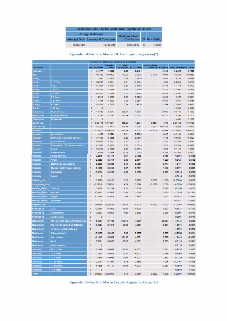
Appendix 54-Portfolio Macro LR Test Logistic regression(2)

Appendix 55-Portfolio Macro Logistic Regression Output(2)

Appendix 56-Portfolio Macro Stepwise Selection Probit Regression

Appendix 57-Portfolio Macro-LR Test Probit Regression(1)

 

 

Appendix 58-Portfolio Macro-Probit Regression Output(2)

Appendix 59-Portfolio Macro –LR Test Probit Regression(2)

 

 

Appendix 60-Portfolio Macro -Probit Regression Output (2)

0.5

Model Sample TN FN TP FP Sensitivity Specificity Misclass KS AUROC AR Brier Score

Logit1 training 19546 1526 1868 385 0.55 0.981 0.082 0.676 0.916 0.832 0.064

Logit1 validation 5510 464 558 132 0.546 0.977 0.089 0.669 0.914 0.828 0.068

Logit1 test 2757 214 305 56 0.588 0.98 0.081 0.674 0.908 0.817 0.067

Logit 2 training 19547 1528 1866 384 0.55 0.981 0.082 0.671 0.914 0.827 0.065

Logit 2 validation 5512 472 550 130 0.538 0.977 0.09 0.664 0.911 0.822 0.069

Logit 2 test 2757 221 298 56 0.574 0.98 0.083 0.67 0.907 0.814 0.068

Probit 1 training 19593 1620 1774 338 0.523 0.983 0.084 0.674 0.915 0.83 0.066

Probit 1 validation 5533 492 530 109 0.519 0.981 0.09 0.668 0.913 0.825 0.069

Probit 1 test 2764 235 284 49 0.547 0.983 0.085 0.667 0.908 0.816 0.068

Probit2 training 19594 1639 1755 337 0.517 0.983 0.085 0.669 0.912 0.825 0.067

Probit2 validation 5529 501 521 113 0.51 0.98 0.092 0.662 0.91 0.819 0.071

Probit2 test 2765 236 283 48 0.545 0.983 0.085 0.666 0.907 0.814 0.069

NN1 training 19537 1296 2098 394 0.618 0.98 0.072 0.709 0.933 0.867 0.056

NN1 validation 5500 394 628 142 0.614 0.975 0.08 0.706 0.923 0.846 0.062

NN1 test 2747 196 323 66 0.622 0.977 0.079 0.704 0.92 0.84 0.061

NN2 training 19557 1294 2100 374 0.619 0.981 0.072 0.714 0.936 0.872 0.055

NN2 validation 5502 380 642 140 0.628 0.975 0.078 0.7 0.927 0.855 0.061

NN2 test 2754 181 338 59 0.651 0.979 0.072 0.704 0.928 0.856 0.059

Confusion Matrix Goodness of fit

 

Appendix 61-Portfolio Macro Goodness of Fit Results

 

Appendix 62-Portfolio Macro CAP Curve 

 

Confusion Matrix Goodness of Fit

Model Sample TN FN TP FP Sensitivity Specificity Misclass KS AUROC AR Brier Score

Logit 2 test 0.22% -3.49% 2.76% -9.68% 2.76% 0.22% -4.81% 1.40% 0.43% 0.96% -3.72%

Logit 2 training 0.13% -4.38% 3.90% -6.11% 3.90% 0.13% -4.73% 0.85% 0.39% 0.86% -3.23%

Logit 2 validation 0.02% -3.08% 2.80% -0.76% 2.80% 0.02% -2.59% -0.74% 0.07% 0.15% -1.89%

Logit1 test 0.07% -4.46% 3.39% -3.45% 3.39% 0.07% -4.26% 0.03% 0.47% 1.04% -4.01%

Logit1 training 0.06% -3.42% 2.98% -3.02% 2.98% 0.06% -3.34% 1.30% 0.48% 1.07% -3.47%

Logit1 validation -0.31% -4.13% 3.72% 14.78% 3.72% -0.31% -0.50% -0.59% 0.19% 0.43% -2.32%

NN1 test 0.18% 4.81% -2.71% -7.04% -2.71% 0.18% 1.55% 2.88% 0.78% 1.73% -5.39%

NN1 training 0.33% -6.22% 4.27% -14.16% 4.27% 0.33% -8.20% 4.05% 1.40% 3.08% -9.63%

NN1 validation 0.09% -1.01% 0.64% -3.40% 0.64% 0.09% -1.65% 3.89% 0.80% 1.76% -4.29%

NN2 test 0.51% -8.12% 4.97% -19.18% 4.97% 0.51% -11.11% 2.72% 1.32% 2.91% -9.63%

NN2 training 0.20% -5.34% 3.60% -9.44% 3.60% 0.20% -6.29% 3.86% 0.94% 2.04% -8.08%

NN2 validation 0.07% -8.21% 5.59% -2.78% 5.59% 0.07% -6.81% 0.56% 0.87% 1.91% -5.89%

Probit 1 test 0.04% -5.62% 5.19% -2.00% 5.19% 0.04% -5.02% 0.21% 0.46% 1.03% -4.22%

Probit 1 training -0.10% -4.31% 4.29% 5.96% 4.29% -0.10% -2.68% 1.47% 0.45% 0.99% -3.49%

Probit 1 validation -0.11% -5.20% 5.37% 5.83% 5.37% -0.11% -3.38% -0.40% 0.14% 0.30% -2.64%

Probit2 test 0.25% -6.72% 6.39% -12.73% 6.39% 0.25% -7.79% 1.44% 0.43% 0.96% -3.81%

Probit2 training 0.10% -5.70% 5.98% -5.34% 5.98% 0.10% -5.64% 0.82% 0.34% 0.77% -3.20%

Probit2 validation -0.07% -6.36% 6.98% 3.67% 6.98% -0.07% -4.66% -0.68% 0.01% 0.03% -2.14% Appendix 63-Macroeconomic improvement on portfolio models

 

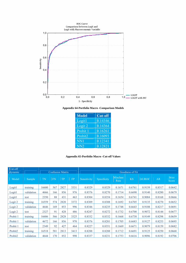
Appendix 64-Portfolio Macro -Comparison Models

Model Cut-off Logit1 0.14346Logit 2 0.14364Probit 1 0.16261Probit2 0.16093NN1 0.12341NN2 0.12821

Appendix 65-Portfolio Macro -Cut-off Values

Cut-off dynamic Confusion Matrix Goodness of Fit

Model Sample TN FN TP FP Sensitivity Specificity Misclass Rate KS AUROC AR Brier

Score

Logit1 training 16600 567 2827 3331 0.8329 0.8329 0.1671 0.6761 0.9159 0.8317 0.0642

Logit1 validation 4666 166 856 976 0.8376 0.8270 0.1714 0.6690 0.9140 0.8280 0.0679

Logit1 test 2350 88 431 463 0.8304 0.8354 0.1654 0.6741 0.9084 0.8168 0.0666

Logit 2 training 16559 574 2820 3372 0.8309 0.8308 0.1692 0.6705 0.9135 0.8270 0.0652

Logit 2 validation 4646 169 853 996 0.8346 0.8235 0.1748 0.6643 0.9108 0.8217 0.0691

Logit 2 test 2327 91 428 486 0.8247 0.8272 0.1732 0.6700 0.9072 0.8144 0.0677

Probit 1 training 16606 566 2828 3325 0.8332 0.8332 0.1668 0.6738 0.9149 0.8298 0.0659

Probit 1 validation 4672 166 856 970 0.8376 0.8281 0.1705 0.6683 0.9127 0.8253 0.0695

Probit 1 test 2349 92 427 464 0.8227 0.8351 0.1669 0.6671 0.9079 0.8159 0.0682

Probit2 training 16518 581 2813 3413 0.8288 0.8288 0.1712 0.6691 0.9125 0.8250 0.0668

Probit2 validation 4644 170 852 998 0.8337 0.8231 0.1753 0.6616 0.9096 0.8192 0.0706

 

 

=5

odel ample N N P P Sensitivity Specificity Miscalss

Rate KS AUROC AR Brier Score

ogit1 raining 0.07% 0.95% .83% .27% .83% 0.07% 0.10% .00% .00% .00% 0.01%

ogit1 alidation 0.05% 1.24% .12% .61% .12% 0.05% 0.50% .00% .00% .00% 0.04%

ogit1 est .11% 5.36% .07% 5.17% .07% .11% 5.32% 0.02% .48% .06% 4.07%

ogit 2 raining .09% 5.38% .79% 4.16% .79% .09% 5.13% .85% .39% .86% 3.24%

ogit 2 alidation 0.11% 3.29% .99% .58% .99% 0.11% 1.62% 0.74% .07% .15% 1.89%

ogit 2 est .15% 5.68% .48% 6.45% .48% .15% 5.84% .40% .43% .96% 3.70%

robit 1 raining 0.06% 1.54% .53% .76% .53% 0.06% 0.70% .00% .00% .00% 0.03%

robit 1 alidation 0.05% 0.77% .80% .91% .80% 0.05% 0.16% .00% .00% .00% 0.05%

robit 1 est 0.04% 8.43% .78% .00% .78% 0.04% 6.69% .21% .47% .05% 4.28%

robit2 raining .04% 7.02% .37% 1.97% .37% .04% 6.16% .82% .34% .77% 3.21%

robit2 alidation 0.09% 6.92% .60% .59% .60% 0.09% 4.97% 0.68% .01% .03% 2.15%

robit2 est .25% 7.51% .14% 12.73% .14% .25% 8.44% .44% .43% .96% 3.80%

N1 raining 0.04% 10.13% .96% .53% .96% 0.04% 7.22% .26% .87% .09% 10.08%

N1 alidation 0.20% 5.28% .37% .48% .37% 0.20% 1.83% .67% .63% .58% 6.30%

N1 est 0.04% 0.53% .30% .41% .30% 0.04% .00% .42% .51% .34% 5.02%

N2 raining .23% 5.85% .95% 10.65% .95% .23% 6.97% .28% .96% .09% 7.70%

N2 alidation .09% 7.97% .43% 3.47% .43% .09% 6.81% .89% .95% .08% 6.61%

N2 est .47% 2.03% .24% 17.81% .24% .47% 6.30% .07% .51% .33% 8.58%

=10

odel ample N N P P Sensitivity Specificity Miscalss

Rate KS AUROC AR Brier Score

ogit1 raining .11% .59% 2.26% 5.54% 2.26% .11% .96% 1.90% 0.46% 1.02% .96%

ogit1 alidation .00% .31% 2.97% .00% 2.97% .00% .67% 1.34% 0.32% 0.70% .02%

ogit1 est 0.18% .46% 3.39% .62% 3.39% 0.18% .32% 1.03% 0.52% 1.16% .36%

ogit 2 raining .09% 5.38% .79% 4.16% .79% .09% 5.13% .85% .39% .86% 3.24%

ogit 2 alidation 0.11% 3.29% .99% .58% .99% 0.11% 1.62% 0.74% .07% .15% 1.89%

ogit 2 est .15% 5.68% .48% 6.45% .48% .15% 5.84% .40% .43% .96% 3.70%

robit 1 raining 0.06% 1.54% .53% .76% .53% 0.06% 0.70% .00% .00% .00% 0.03%

robit 1 alidation 0.05% 0.77% .80% .91% .80% 0.05% 0.16% .00% .00% .00% 0.05%

Probit2 test 2328 93 426 485 0.8208 0.8276 0.1735 0.6664 0.9069 0.8138 0.0693

NN1 training 16993 500 2894 2938 0.8527 0.8526 0.1474 0.7092 0.9335 0.8669 0.0564

NN1 validation 4772 153 869 870 0.8503 0.8458 0.1535 0.7058 0.9232 0.8464 0.0625

NN1 Test 2391 85 434 422 0.8362 0.8500 0.1522 0.7042 0.9201 0.8401 0.0615

NN2 Trening 17019 495 2899 2912 0.8542 0.8539 0.1461 0.7144 0.9361 0.8721 0.0552

NN2 validation 4797 166 856 845 0.8376 0.8502 0.1517 0.6997 0.9273 0.8547 0.0610

NN2 Test 2404 79 440 409 0.8478 0.8546 0.1465 0.7037 0.9278 0.8556 0.0587

Appendix 66-Portfolio Macro -Dynamic Cut-off

robit 1 est .14% 6.02% .56% 8.00% .56% .14% 6.35% 0.26% .31% .70% 2.69%

robit2 raining .04% 7.02% .37% 1.97% .37% .04% 6.16% .82% .34% .77% 3.21%

robit2 alidation 0.09% 6.92% .60% .59% .60% 0.09% 4.97% 0.68% .01% .03% 2.15%

robit2 est .25% 7.51% .14% 12.73% .14% .25% 8.44% .44% .43% .96% 3.80%

N1 raining 0.05% 10.13% .96% .96% .96% 0.05% 7.12% .26% .86% .07% 10.09%

N1 alidation 0.20% 5.28% .37% .48% .37% 0.20% 1.83% .79% .62% .57% 6.26%

N1 est 0.07% 0.53% .30% .82% .30% 0.07% .39% .99% .50% .31% 5.00%

N2 raining .15% 6.58% .44% 7.26% .44% .15% 6.74% .45% .96% .09% 7.56%

N2 alidation 0.02% 7.73% .26% .69% .26% 0.02% 5.56% .35% .96% .10% 6.49%

N2 est .33% 3.05% .86% 12.33% .86% .33% 5.56% .85% .52% .35% 8.67%

=15

odel ample N N P P Sensitivity Specificity Miscalss

Rate KS AUROC AR Brier Score

ogit1 raining 0.07% 0.95% .83% .27% .83% 0.07% 0.10% .00% .00% .00% 0.01%

ogit1 alidation 0.05% 1.24% .12% .61% .12% 0.05% 0.50% .00% .00% .00% 0.04%

ogit1 est .11% 5.36% .07% 5.17% .07% .11% 5.32% 0.02% .48% .06% 4.07%

ogit 2 raining .09% 5.38% .79% 4.16% .79% .09% 5.13% .85% .39% .86% 3.24%

ogit 2 alidation 0.11% 3.29% .99% .58% .99% 0.11% 1.62% 0.74% .07% .15% 1.89%

ogit 2 est .15% 5.68% .48% 6.45% .48% .15% 5.84% .40% .43% .96% 3.70%

robit 1 raining 0.06% 1.54% .53% .76% .53% 0.06% 0.70% .00% .00% .00% 0.03%

robit 1 alidation 0.05% 0.77% .80% .91% .80% 0.05% 0.16% .00% .00% .00% 0.05%

robit 1 est 0.04% 8.43% .78% .00% .78% 0.04% 6.69% .21% .47% .05% 4.28%

robit2 raining .04% 7.02% .37% 1.97% .37% .04% 6.16% .82% .34% .77% 3.21%

robit2 alidation 0.09% 6.92% .60% .59% .60% 0.09% 4.97% 0.68% .01% .03% 2.15%

robit2 est .25% 7.51% .14% 12.73% .14% .25% 8.44% .44% .43% .96% 3.80%

N1 raining 0.02% 10.35% .11% .65% .11% 0.02% 7.60% .26% .88% .12% 10.16%

N1 alidation 0.16% 4.27% .72% .12% .72% 0.16% 1.47% .58% .65% .64% 6.39%

N1 est .07% 1.60% .90% 2.82% .90% .07% 1.94% .81% .61% .55% 5.35%

N2 raining .15% 6.58% .44% 7.26% .44% .15% 6.74% .45% .96% .09% 7.56%

N2 alidation 0.02% 7.73% .26% .69% .26% 0.02% 5.56% .35% .96% .10% 6.49%

N2 est .33% 3.05% .86% 12.33% .86% .33% 5.56% .85% .52% .35% 8.67% Appendix 67-Cost Comparison -Model Improvement vs. Portfolio Results

Spiegelhalter Test LOGIT1 LOGIT2 PROBIT1 PROBIT2 NN1 NN2Port 0.7605 0.7330 0.1932 0.1773 0.8992 0.2235Macro 0.7852 0.6458 0.1626 0.1133 0.2602 0.5743  

Appendix 68-Spiegelhalter Test

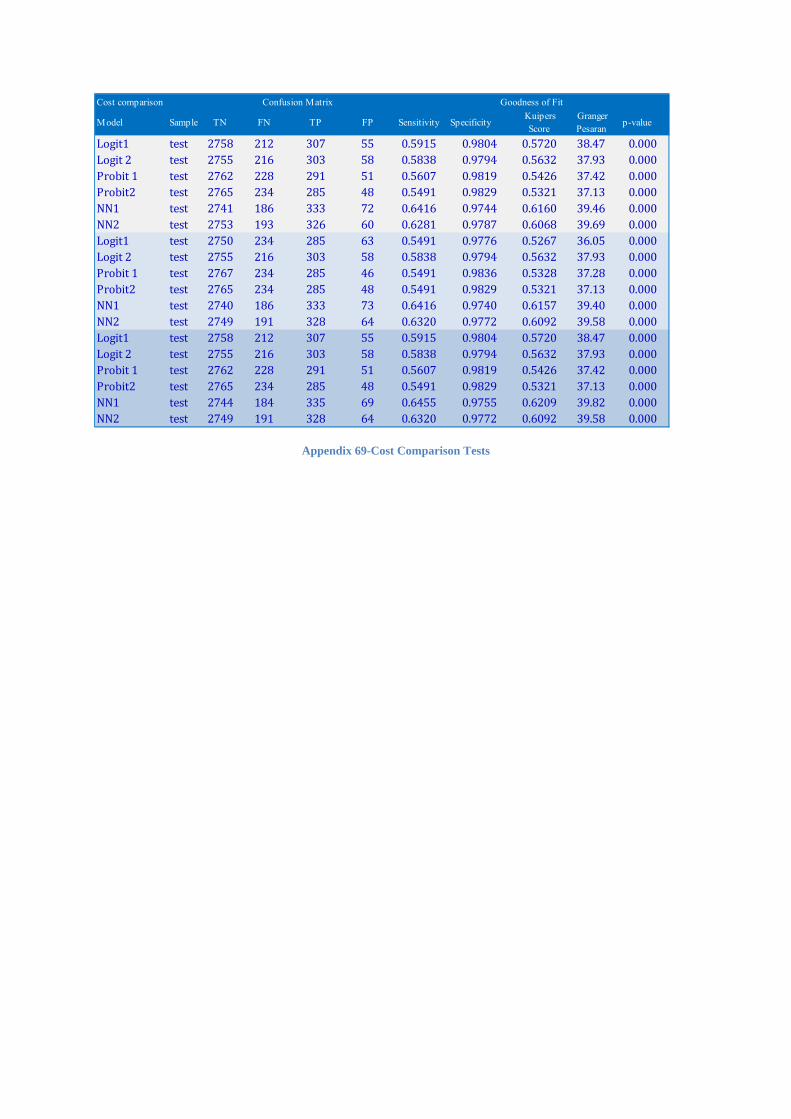
Cost comparison

Model Sample TN FN TP FP Sensitivity Specificity Kuipers

Score Granger Pesaran

p-value

Logit1 test 2758 212 307 55 0.5915 0.9804 0.5720 38.47 0.000Logit 2 test 2755 216 303 58 0.5838 0.9794 0.5632 37.93 0.000Probit 1 test 2762 228 291 51 0.5607 0.9819 0.5426 37.42 0.000Probit2 test 2765 234 285 48 0.5491 0.9829 0.5321 37.13 0.000NN1 test 2741 186 333 72 0.6416 0.9744 0.6160 39.46 0.000NN2 test 2753 193 326 60 0.6281 0.9787 0.6068 39.69 0.000Logit1 test 2750 234 285 63 0.5491 0.9776 0.5267 36.05 0.000Logit 2 test 2755 216 303 58 0.5838 0.9794 0.5632 37.93 0.000Probit 1 test 2767 234 285 46 0.5491 0.9836 0.5328 37.28 0.000Probit2 test 2765 234 285 48 0.5491 0.9829 0.5321 37.13 0.000NN1 test 2740 186 333 73 0.6416 0.9740 0.6157 39.40 0.000NN2 test 2749 191 328 64 0.6320 0.9772 0.6092 39.58 0.000Logit1 test 2758 212 307 55 0.5915 0.9804 0.5720 38.47 0.000Logit 2 test 2755 216 303 58 0.5838 0.9794 0.5632 37.93 0.000Probit 1 test 2762 228 291 51 0.5607 0.9819 0.5426 37.42 0.000Probit2 test 2765 234 285 48 0.5491 0.9829 0.5321 37.13 0.000NN1 test 2744 184 335 69 0.6455 0.9755 0.6209 39.82 0.000NN2 test 2749 191 328 64 0.6320 0.9772 0.6092 39.58 0.000

Confusion Matrix Goodness of Fit

 

Appendix 69-Cost Comparison Tests