Automated lead scoring system: a case study of a Portuguese startup

José Diogo da Silva Santos Rodrigues

Internship Report

Master in Management

Supervised by Pedro José Ramos Moreira de Campos

Internship Supervisor Tiago Alberto Campos Paiva

2020

i

Acknowledgments

First, I would like to express my sincere gratitude to my supervisor, Professor Pedro

Campos for motivating me and giving me the confidence to pursue a research within a topic

out of my comfort zone, even though I had no previous knowledge about it before doing this

report. Thank you for your support, expertise and for opening my horizons for such an

interesting and present matter.

Second, I would like to thank HUUB and Tiago Paiva for welcoming me throughout my

internship period where I acquired valuable skills to my future professional career.

Third, I am deeply thankful for my family for making my academic journey the better one

and providing me everything to be a successful human being. Without your support I would

not be who I am today. I hope this achievement makes you proud.

I would also like to thank my friends who have always supported me throughout this

academic journey and along the realization of this research namely to Ana, Pedro and Wilson.

ii

Resumo

Na generalidade dos contextos de negócio, as oportunidades de venda são monitorizadas

através de um pipeline de vendas, normalmente utilizando ferramentas de automação de vendas,

como plataformas de Customer Relationship Management (CRM). Estes sistemas de CRM

armazenam uma grande quantidade de dados e as empresas estão cada vez mais a tomar

consciência da importância que este facto pode ter nos seus negócios, como por exemplo para

suportar decisões de negócios, como a identificação de potenciais novos clientes e a seleção de

quais potenciais clientes contactar em primeiro lugar. A abordagem predominante usada pelas

organizações para lidar com este problema consiste no lead scoring manual (tradicional), com a

elaboração de um lead scorecard para introduzir nas plataformas de CRM já mencionadas. No

entanto, a enorme quantidade de dados armazenados nos sistemas de CRM pode ser usada

para priorizar que leads contactar em primeiro lugar, estimando a probabilidade de uma lead se

converter num cliente, usando predictive analytics e machine learning como suporte ao lead scoring.

Este relatório de estágio consiste num caso de estudo de uma startup portuguesa sugerindo

duas abordagens relativamente à problemática de lead scoring. É apresentada uma solução

automatizada, tendo como base conceitos de machine learning através da aplicação de algoritmos

de classificação supervisionados, bem como uma abordagem manual como complemento à

abordagem automatizada.

PALAVRAS-CHAVE: Customer Relationship Management; Lead Scoring; Predictive Analytics;

Machine Learning

iii

Abstract

In most business contexts, sales opportunities are tracked within a sales pipeline, often

using sales force automation tools, such as Customer Relationship Management (CRM)

platforms. Those CRM systems store a large amount of data and companies are becoming

aware of the importance that it can have on their businesses to support business decisions,

such as the identification of potential new customers and the selection of which sales leads to

pursue firstly. The mainstream approach used by organizations to address this fact consists on

manual (traditional) lead scoring, with the design of a lead scorecard to embed on the already

mentioned CRM platforms. In addition, the enormous amount of data stores on those CRM

systems can be used to prioritize which leads to contact firstly, by estimating a lead likelihood

to convert into a customer, by using predictive analytics and machine learning to perform lead

scoring.

This internship report consists of a case study of a Portuguese startup with the purpose of

providing two solutions regarding the topic of lead scoring. A machine learning assisted

solution with the application of supervised classification algorithms and a manual approach as

a complement to the automated one are presented.

KEY WORDS: Customer Relationship Management; Lead Scoring; Predictive Analytics;

Machine Learning

iv

Contents

1. Introduction ..................................................................................................................................... 1

1.1. Company Overview ................................................................................................................ 2

1.2. Research Objective ................................................................................................................. 3

1.3. Structure of the report............................................................................................................ 4

2. Literature review .............................................................................................................................. 5

2.1. Customer Relationship Management (CRM) ...................................................................... 5

2.2. Data mining applications in CRM ........................................................................................ 7

2.3. Customer Acquisition Process – Sales Funnel ................................................................... 8

2.4. Prioritization of leads ........................................................................................................... 10

2.5. Traditional lead scoring ........................................................................................................ 11

2.6. Automated lead scoring ....................................................................................................... 13

2.7. Predictive Analytics .............................................................................................................. 14

2.7.1. Supervised learning vs Unsupervised learning ......................................................... 14

2.7.2. Supervised classification algorithms........................................................................... 15

2.7.3. Class Imbalance ............................................................................................................ 17

2.7.4. Model’s performance ................................................................................................... 18

2.8. Similar studies ........................................................................................................................ 22

3. Methodological Aspects ............................................................................................................... 29

3.1. Phases/Steps of the study .................................................................................................... 30

4. Empirical study .............................................................................................................................. 32

4.1. Business Understanding ....................................................................................................... 32

4.2. Data Understanding .............................................................................................................. 38

4.2.1. General Overview ......................................................................................................... 38

v

4.2.2. Won/Lost leads ............................................................................................................ 39

4.2.3. First feature selection ................................................................................................... 40

4.2.4. Exploratory Data Analysis .......................................................................................... 41

4.3. Data Preparation ................................................................................................................... 58

4.3.1. Final feature selection .................................................................................................. 58

4.3.2. Missing Values............................................................................................................... 59

4.3.3. Data Transformation ................................................................................................... 61

4.3.4. Label creation ................................................................................................................ 62

4.4. Modelling ............................................................................................................................... 63

4.5. Evaluation .............................................................................................................................. 65

5. Discussion ...................................................................................................................................... 68

6. Manual approach – Scorecard ..................................................................................................... 74

6.1. Automated lead scoring system vs Manual lead scoring scorecard ............................... 79

7. Final Remarks ................................................................................................................................ 82

7.1. Conclusions ............................................................................................................................ 82

7.2. Limitations and Further Suggestions ................................................................................. 83

References ............................................................................................................................................... 85

Appendix A: Features Description ..................................................................................................... 89

Appendix B: One-Hot Encoding ........................................................................................................ 91

Appendix C: RapidMiner Modelling Process .................................................................................... 93

Appendix D: Feature Relevance .......................................................................................................... 97

Appendix E: HUUB’s Lead Scoring Scorecard ................................................................................ 98

vi

List of Graphs

Graph 1 - Won vs Lost leads ............................................................................................................... 40

Graph 2 - Won vs Lost leads by Deal Source ................................................................................... 41

Graph 3 - Won vs Lost leads by Brand Segment ............................................................................. 42

Graph 4 - HUUB's actual/past clients by Country .......................................................................... 43

Graph 5 - Won vs Lost leads by Main Market(s).............................................................................. 45

Graph 6 - Won vs Lost leads by Sales Channel(s) ............................................................................ 46

Graph 7 - HUUB's actual/past clients by Ecommerce platform ................................................... 47

Graph 8 - Won vs Lost leads by Production venue ......................................................................... 48

Graph 9 - Won vs Lost leads by Product Category.......................................................................... 50

Graph 10 - Won vs Lost leads by Brand Type .................................................................................. 51

Graph 11 - Won vs Lost leads by number of Instagram Followers .............................................. 52

Graph 12 - Won vs Lost leads by Price per Item ............................................................................. 54

Graph 13 - Won vs Lost leads by Brand Tier ................................................................................... 56

vii

List of Tables

Table 1 - Summary of similar studies regarding the topic of predictive lead scoring .................. 28

Table 2 - Deal Stages of actual/past clients (Won) and Non Clients (Lost leads) ....................... 39

Table 3 - Won vs Lost leads by Deal Source ..................................................................................... 41

Table 4 - Won vs Lost leads by Brand Segment ............................................................................... 42

Table 5 - Won vs Lost leads by Main Market(s) ............................................................................... 45

Table 6 - Won vs Lost leads by Sales Channel(s) ............................................................................. 46

Table 7 - Lost leads by most represented Ecommerce platforms .................................................. 48

Table 8 - Won vs Lost leads by Production venue ........................................................................... 49

Table 9 - Won vs Lost leads by Product Category ........................................................................... 50

Table 10 - Won vs Lost leads by Brand Type ................................................................................... 51

Table 11 - Won vs Lost leads by number of Instagram followers ................................................. 52

Table 12 - Won vs Lost leads by Price per Item ............................................................................... 54

Table 13 - Common values among Lost leads in regard to Amount (ARR) ................................ 55

Table 14 - Won vs Lost leads by Brand Tier ..................................................................................... 56

Table 15 - Feature Selection ................................................................................................................. 58

Table 16 - Number of observations with missing values by feature and class ............................. 60

Table 17 - Number of observations with and without missing values by class............................ 60

Table 18 - Data quality: Categorical Variables................................................................................... 61

Table 19 - Performance metrics of the scenario I ............................................................................ 65

Table 20 - Precision and Recall of the scenario I ............................................................................. 65

Table 21 - Performance metrics of the scenario II.......................................................................... 66

Table 22 - Precision and Recall of the scenario II ............................................................................ 66

Table 23 - Performance metrics of the scenario III ......................................................................... 66

viii

Table 24 - Precision and Recall of the scenario III .......................................................................... 67

Table 25 - Performance metrics of the scenario IV ......................................................................... 67

Table 26 - Precision and Recall of the scenario IV .......................................................................... 67

Table 27 - Variables description .......................................................................................................... 90

Table 28 – Examples of feature transformation of the feature Main Market(s) .......................... 91

Table 29 – Examples of feature transformation of the feature Sales Channel(s) ........................ 91

Table 30 - Examples of feature transformation of the feature Production .................................. 91

Table 31 - Examples of feature transformation of the feature Product Category ....................... 92

Table 32 - Examples of feature transformation of the feature Brand Type ................................. 92

Table 33 - Feature relevance ................................................................................................................ 97

Table 34 - HUUB's Lead Scoring Scorecard ................................................................................... 100

ix

List of Figures

Figure 1 - HUUB's ecosystem ............................................................................................................... 3

Figure 2 - Common sales funnel framework (adapted from Järvinen and Taiminen (2016)) ...... 9

Figure 3 - An example of manual lead scorecard (adapted from Duncan and Elkan (2015)).... 12

Figure 4 - Confusion matrix (Abbott, 2014)...................................................................................... 19

Figure 5 - An example of ROC curve (Kuhn & Johnson, 2013) ................................................... 21

Figure 6 - Performance measures (Abbott, 2014)............................................................................. 22

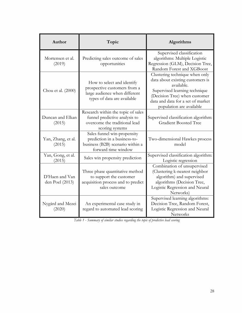
Figure 7 - CRISP-DM Process Model for Data Mining projects (Wirth & Hipp, 2000)............ 30

Figure 8 - HUUB's sales pipeline ........................................................................................................ 33

Figure 9 - ROC of the best overall performing model .................................................................... 72

Figure 10 - RapidMiner modelling process within the scenario I (dataset without missing values

combined with the undersampling technique) .................................................................................. 93

Figure 11 - RapidMiner modelling process within the scenario II (dataset without missing

values combined with the SMOTE technique) ................................................................................. 94

Figure 12 - RapidMiner modelling process within the scenario III (dataset with missing values

combined with the undersampling technique) .................................................................................. 95

Figure 13 - RapidMiner modelling process within the scenario IV (dataset with missing values

combined with the oversampling technique) .................................................................................... 96

1

1. Introduction

We are living times of deep changes, promoted by digitalization, information and

communications technology, machine learning, robotics and artificial intelligence (AI). A new

era that many labelled as the fourth industrial revolution (Syam & Sharma, 2018). In the most

recent years, companies have used the surge of the amount of data collected by them to

improve their businesses, since it can provide useful insights. According to the ones of

economic and business areas, this will shift the paradigm of the process of decision making.

Nowadays, new technologies such as AI allow computers to solve problems that years ago

required a lot of human intervention (Paschen, Wilson, & Ferreira, 2020). Business decisions

will no longer be only human based but instead supported by computers and mathematical and

statistical techniques. Data driven decisions are better business decisions. With that being said,

it is easy to conclude that using data to solve business problems will become the standard in

the future (Brynjolfsson & McElheran, 2016).

Particularly, the customer acquisition process, namely business-to-business (B2B) selling,

has drastically evolved along the years, from in person meetings with potential customers to

customer relationship management (CRM) systems (Yan, Zhang, et al., 2015).

A critical concern related to the customer acquisition process is which sales lead to contact

in the first place. Despite the fact that it is possible to observe an emerging trend practiced by

some companies that aim to use this new technologies to support the customer acquisition

process, this initial step of the process is still a human-centric-process, which may not be the

most efficient one (Paschen et al., 2020).

In this report, it is aimed to provide an automated solution to a Portuguese startup

regarding the topic of lead scoring. Lead scoring consists on ranking sales leads according to

their perceived value to the organization and the probability of becoming a customer. With a

lead scoring system, the organization under analysis can select which leads the sales

department should contact in the first place, being the first ones the leads that have the highest

probability of resulting in a successful sale. In order to achieve that, supervised learning

classification algorithms are applied as the foundation of the automated solution. Moreover,

2

after analyzing the company’s data extracted from its CRM platform, a manual solution (lead

scorecard) is also suggested.

By developing a machine learning assisted solution to the company under analysis, the sales

department can accurately know in advance if a lead has a higher probability of becoming a

customer and, given that, it provides the possibility of allocating resources to those leads that

have a higher quality and propensity of resulting in a successful sale, which is expected to have

a major impact on a company’s business.

While the tools to support this process in an automated way are easily available to most of

the companies and individuals, we have found very few academic studies regarding to the topic

of applying these new technologies, namely predictive analytics as a sub-domain of machine

learning, to pursue lead scoring. Thus, it is expected that this report also contributes to close

this gap by explaining how machine learning can be the foundation to lead scoring.

1.1. Company Overview

HUUB is a startup founded in 2015 by four Portuguese that offers an end-to-end logistic

platform for distinctive fashion brands. The company aims to manage small and medium

fashion brands’ supply chain as a whole, from its suppliers to its final customers, regarding not

only ecommerce operations but also wholesale operations. The company ecosystem is

composed of brands, end-users (retailers and customers), suppliers, carriers and other partners.

This solution enables small independent brands to avoid unnecessary waste of time, money

and energy, allowing them to focus only on their product development, sales, and marketing.

Hence, HUUB’s clients can focus on their core business: to design their collections and to

boost their sales, since all the complexity of the supply chain is managed by HUUB. HUUB

has named itself as “Brand Accelerators” since their clients can focus on what is more

important to them, their core business (design collections) and delegate the complexity of

managing the logistics to HUUB. It is a win-win situation: if HUUB’s clients grow, HUUB

grows too.

3

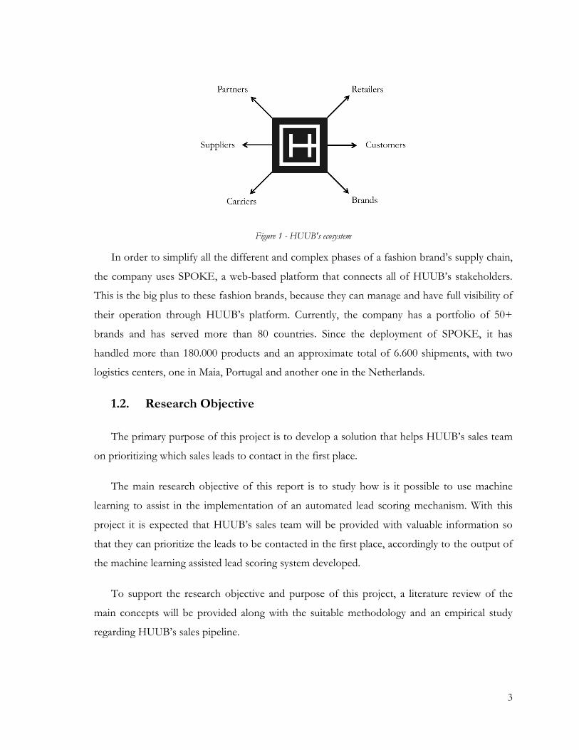
Figure 1 - HUUB's ecosystem

In order to simplify all the different and complex phases of a fashion brand’s supply chain,

the company uses SPOKE, a web-based platform that connects all of HUUB’s stakeholders.

This is the big plus to these fashion brands, because they can manage and have full visibility of

their operation through HUUB’s platform. Currently, the company has a portfolio of 50+

brands and has served more than 80 countries. Since the deployment of SPOKE, it has

handled more than 180.000 products and an approximate total of 6.600 shipments, with two

logistics centers, one in Maia, Portugal and another one in the Netherlands.

1.2. Research Objective

The primary purpose of this project is to develop a solution that helps HUUB’s sales team

on prioritizing which sales leads to contact in the first place.

The main research objective of this report is to study how is it possible to use machine

learning to assist in the implementation of an automated lead scoring mechanism. With this

project it is expected that HUUB’s sales team will be provided with valuable information so

that they can prioritize the leads to be contacted in the first place, accordingly to the output of

the machine learning assisted lead scoring system developed.

To support the research objective and purpose of this project, a literature review of the

main concepts will be provided along with the suitable methodology and an empirical study

regarding HUUB’s sales pipeline.

4

1.3. Structure of the report

Besides this section, where an introduction to the topic of this report and the purpose of

this project are presented, this report is structured as follows: on section 2, a literature review

on the major concepts of this report is presented, to facilitate the understanding of this project.

Then, on section 3 the steps to pursue the purpose of this project are highlighted. On section

4, the process of developing the machine learning assisted lead scoring system is outlined,

followed by section 5 where the consequent analysis of the algorithms applied is addressed and

the results obtained in the empirical study as a whole are discussed. The explanation of the

manual lead scorecard designed can be found in section 6. Finally, on section 7 the conclusions

and future suggestions and limitations regarding this research are discussed.

5

2. Literature review

This chapter aims to deliver an easy understanding of the main concepts regarding the

problem and topic under analysis. On section 2.1, the concept of Customer Relationship

Management (CRM) is addressed. On section 2.2, some brief approach of data mining

applications in CRM is provided. On section 2.3 the topic of customer acquisition and the

sales funnel framework are discussed. Section 2.4 comprises an approach of prioritization of

leads, followed by the concept of traditional lead scoring in 2.5. On section 2.6 the concept of

automated lead scoring is addressed and section 2.7 addresses the foundation of predictive lead

scoring: predictive analytics. Finally, on section 2.8 a comprehension of academic similar

studies on this topic is presented.

2.1. Customer Relationship Management (CRM)

The concept of Customer Relationship Management (CRM) is frequently mentioned in

marketing literature. The interest in this concept arises in 1990 and it becomes widely

recognized. However, there is no consensus regarding its definition (Ngai, 2005). Some

definitions are provided in the following sentences. As per Swift (2001) CRM is an “enterprise

approach to understanding and influencing customer behavior through meaningful

communications in order to improve customer acquisition, customer retention, customer

loyalty, and customer profitability”. According to Kincaid (2003), CRM is “the strategic use of

information, processes, technology and people to manage the customer’s relationship with

your company (Marketing, Sales, Services, and Support) across the whole customer life cycle”.

Another definition provided by Parvatiyar and Sheth (2001) states that “Customer Relationship

Management is a comprehensive strategy and process of acquiring, retaining, and partnering

with selective customers to create superior value for the company and the customer. It

involves the integration of marketing, sales, customer service, and the supply-chain functions

of the organization to achieve greater efficiencies and effectiveness in delivering customer

value”. CRM includes processes and systems to support a business strategy to build long term,

profitable relationships with specific customers. Any CRM strategy is built with the foundation

of customer data and information technology (Ngai, Xiu, & Chau, 2009). Generally all of

CRM’s definitions emphasize the relevance of understanding it as a process of acquiring and

6

retaining customers, with the help of business intelligence, to maximize the customer value to

the organization (Ngai et al., 2009). The list could continue, as it is possible to find many

definitions of CRM on academic literature. However, most of them have some concepts in

common such as acquisition and retention of customers and the maximization of long-term

customer value (D’Haen & Van den Poel, 2013).

CRM can be divided into three different levels, from an architecture point of view:

- Operational CRM: refers to the automation of certain business processes (Ngai et al.,

2009);

- Collaborative CRM: employees from different departments can share information

collected and stored at CRM system (Farquad, Ravi, & Raju, 2014);

- Analytical CRM: refers to the analysis of customer characteristics in order to support

organization’s strategy (Ngai et al., 2009).

Also, CRM can also be comprised of four dimensions (Ngai et al., 2009):

- Customer Identification: Involves targeting the ones that are more likely to become

customers in the future or most profitable to the organization. It is also named

Customer Acquisition;

- Customer Attraction: Organizations can focus efforts on the desired customer

segments and allocate resources into attracting the target customer segments;

- Customer Retention: This is the most focused CRM’s dimension on academic literature

and relates to customers’ satisfaction and expectations and to maintain long-term

relationships;

- Customer Development: This dimension involves expansion of transaction intensity,

transaction value and individual customer profitability.

These four dimensions can be seen as a closed and loop cycle. CRM starts with Customer

Identification/Acquisition, followed by Customer Attraction, Customer Retention and

Customer Development.

7

2.2. Data mining applications in CRM

On one hand, the amount of data generated on the entire world is rising as the years go by.

The increasing amount of data available to the companies has created not only challenges but

also opportunities to them. On the other hand, despite the fact that organizations understand

that this amount of data carries knowledge, which is key to support managerial decisions, most

of this valuable knowledge remains hidden (Shaw, Subramaniam, Tan, & Welge, 2001).

Over the last years, there has been a development of customer relationship management

systems and platforms that enable the collection of data relevant to marketing and sales

processes. On top of that, there is an emerging trend of shifting the paradigm of selling to the

usage of those platforms and sales automation systems (Kawas, Squillante, Subramanian, &

Varshney, 2013).

That is when analytical CRM and data mining come into action. Analytical CRM is a

behind-the-scenes process and refers to the analysis of customers’ characteristics, behaviors

and data to support an organization’s strategy. Thus, analytical CRM provides organizations

with the appropriate information to allocate its resources in the most suitable way and to the

targeted group of customers (Ngai et al., 2009).

Many organizations are collecting huge amounts of data daily about current customers,

prospects, suppliers and business partners. But, the incapacity to discover useful information

untapped in the data, prevents organizations from extracting insights and transforming this

data into valuable knowledge (Ngai et al., 2009).

Data mining tools are the mean to analyze this data within the analytical CRM framework.

These tools can enable organizations to extract the untapped but valuable enormous amount

of data. Hence, the usage of data mining tools within the topic of customer relationship

management systems is starting to emerge in the global economy and to positioning itself as a

trend.

According to Shaw et al. (2001) data mining is defined as “the process of searching and

analyzing data in order to find implicit, but potentially useful information. It involves selecting,

exploring and modeling large amounts of data to uncover previously unknown patterns, and

8

ultimately comprehensible information, from large databases.” With statistical, mathematical,

artificial intelligence and machine learning techniques, data mining can help to analyze and

understand a company’s customer portfolio.

Within the context of CRM, data mining can be applied to support decision making and in

some cases forecast the effect of those same decisions. Data mining applications are

transversal to every CRM dimension, as each one of its dimensions can be supported by

different data mining models (Ngai et al., 2009).

However, for the purpose of this report, customer identification (customer acquisition) will

be given more relevance.

2.3. Customer Acquisition Process – Sales Funnel

The part of selling (and inherently buying) is a crucial part of any economic activity, be it a

multinational company or a micro company that operates in the food and beverage sector.

Prior academic literature provides an exhaustive comprehension of the selling process,

however it emphasizes in particular the customer retention dimension, neglecting the customer

acquisition one (Söhnchen & Albers, 2010).

This situation can be explained because customer retention strategies are generally cheaper

than customer acquisition ones. Nonetheless, besides the increasing relevance of customer

retention, customer acquisition is still a crucial domain and should be a priority focus for many

organizations and researchers, as the first stage of the customer life cycle. Startups that intend

to enter a certain market need new customers, since they lack customers. But this is not a

problem of startups only. Even companies in a saturated market have to conquer new

customers, since they will eventually lose customers along the years (Ang & Buttle, 2006;

D’Haen & Van den Poel, 2013).

Customer acquisition can be depicted as a multistage process. The customer acquisition

framework is commonly known as sales pipeline or sales funnel, which is a quite intuitive way

to understand this process, dividing it into stages. This tool is used by most of the companies

to monitor the flow of business opportunities and throughout its analysis is possible to gather

9

some insights regarding how efficiently customer opportunities are moving through the

different stages of the sales pipeline (Patterson, 2007).

Although this tool is called sales pipeline or sales funnel the term is not owned exclusively

by a sales team but also by a marketing department. Marketing departments are responsible for

bringing potential new customers, by creating new content, delivering new messages to the

market and promoting the company and its product/service (Patterson, 2007).

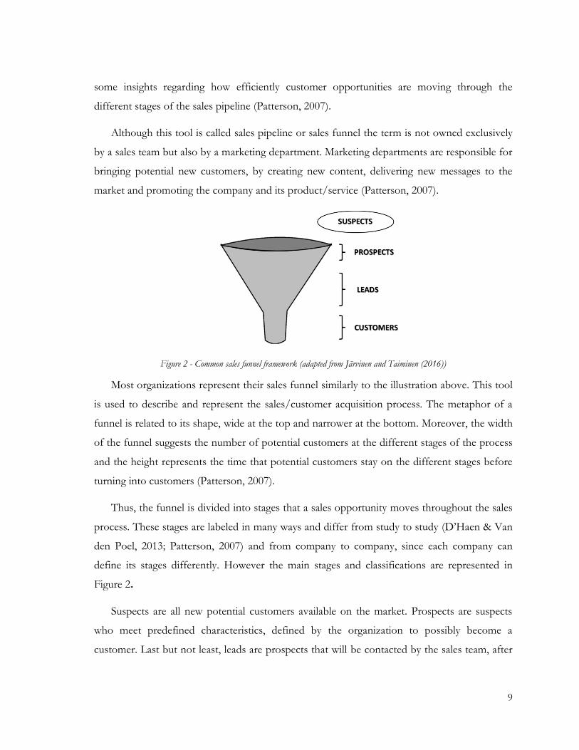
Figure 2 - Common sales funnel framework (adapted from Järvinen and Taiminen (2016))

Most organizations represent their sales funnel similarly to the illustration above. This tool

is used to describe and represent the sales/customer acquisition process. The metaphor of a

funnel is related to its shape, wide at the top and narrower at the bottom. Moreover, the width

of the funnel suggests the number of potential customers at the different stages of the process

and the height represents the time that potential customers stay on the different stages before

turning into customers (Patterson, 2007).

Thus, the funnel is divided into stages that a sales opportunity moves throughout the sales

process. These stages are labeled in many ways and differ from study to study (D’Haen & Van

den Poel, 2013; Patterson, 2007) and from company to company, since each company can

define its stages differently. However the main stages and classifications are represented in

Figure 2.

Suspects are all new potential customers available on the market. Prospects are suspects

who meet predefined characteristics, defined by the organization to possibly become a

customer. Last but not least, leads are prospects that will be contacted by the sales team, after

10

being classified, given any criteria, as the most likely to respond. A sales lead is an entity (a

person in case of business-to-consumer scenario or a business in case of business-to-business

scenario) who may eventually become a customer. Companies generate leads through different

sources: advertising, tradeshows, direct mailings, external agencies and other marketing efforts.

As leads go through different stages, the sales team will qualify them and try to gather the

maximum information, until they get into the desired final stage: becoming a customer

(D’Haen & Van den Poel, 2013; Duncan & Elkan, 2015).

It is important to note that the ideal shape of the funnel and what companies aspire to is

not a funnel. Organizations would prefer its sales funnel to look more like a pipe (which

explains the alternative naming of sales pipeline), where every lead becomes a customer

(Patterson, 2007).

Although this aspiration is not quite realistic, it is possible to widen the bottom of the

funnel, which leads to the following chapter of the literature review.

2.4. Prioritization of leads

To revisit, a lead is an initial potential customer that has not been contacted yet by any

salesperson. Along the so-called lead conversion process (or customer acquisition process)

leads can result in a successful sale (customer) or a failure (lead not converted into customer)

(Duncan & Elkan, 2015).

Since the objective, as it was said before, is to widen the bottom of the sales funnel, that is,

to convert more leads into customers, we will focus on this perspective from now on.

On one hand, the most expensive part of a sales funnel relates to the stage when sales

representatives are pursuing sales opportunities, since these stages request directly workforce

by sales personnel. Yet, in many occasions, there are too many leads to be handled by sales

teams, which assuming that sales personnel work close to its full capacity, implies that it is

impossible for organizations to increase their number of sales calls or sales personnel activities.

On the other hand, an important part of salespersons working time is spent on dealing with a

high volume of low-quality leads that are not going to be converted into customers. That time,

11

used inefficiently, should then be spent with high quality leads that are more likely to become

customers (Duncan & Elkan, 2015).

Furthermore, research states that approximately 20% of a sales representative time is spent

selecting leads to contact and defines this process as the most cumbersome step of the

customer acquisition process. Indeed, if time is spent pursuing low quality leads, that violates

the well-known statement of “time is money” (D’Haen & Van den Poel, 2013).

One could suggest hiring more sales personnel to contact a higher number of leads so that

the probability of pursuing good leads would raise. However, it is not efficient and it is too

much costly to do so.

The only alternative to widen the bottom part of the funnel is to improve the quality of the

leads that are contacted, that is, which leads are the warmest leads, i.e., have the highest chance

to convert. As suggested by Duncan and Elkan (2015), this can be achieved through what the

authors call lead prioritization or lead scoring.

2.5. Traditional lead scoring

Lead scoring refers to the practice of assigning a value to each company’s lead in order to

prioritize company’s outreach. The score can be calculated and based on lead demographic

characteristics (dimension, industry, etc) or on behavioral features (number of website visits,

opened marketing email, etc) and reflects the successful sale potential of the lead (Benhaddou

& Leray, 2017). By scoring the quality of each lead it allows management to better prioritize

and allocate sales personnel, its resources and actions, in face of a high volume of ongoing

leads in a short time period (Yan, Zhang, et al., 2015).

The purpose of lead scoring is to provide sales teams with high quality leads that are more

likely become customers and that represent a highly perceived value to the organization

(D’Haen & Van den Poel, 2013). It consists of ranking the leads to prioritize sales and

marketing efforts and resources towards leads that are more likely to result in successful sales.

Lead scoring guarantees that sales teams are focused on leads that have high perceived value

for the organization and the ones that have low perceived value are not classified as a sales

12

target. By helping sales teams to prioritize which leads to contact firstly, lead scoring enables

the improvement on sales teams’ productivity and efficiency (Duncan & Elkan, 2015).

This concept of lead scoring is also named as manual lead scoring or traditional lead

scoring and is not a new concept. This approach is the mainstream procedure applied by

organizations to prioritize which leads to target. Many companies have a manual lead scoring

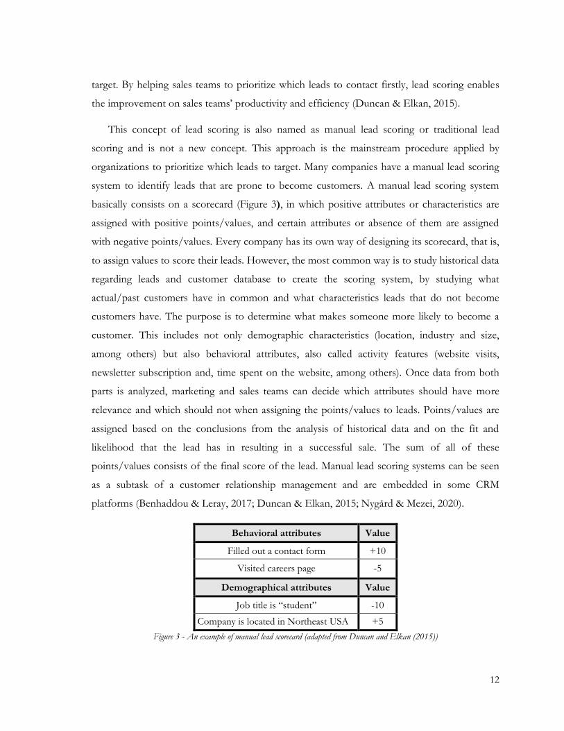
system to identify leads that are prone to become customers. A manual lead scoring system

basically consists on a scorecard (Figure 3), in which positive attributes or characteristics are

assigned with positive points/values, and certain attributes or absence of them are assigned

with negative points/values. Every company has its own way of designing its scorecard, that is,

to assign values to score their leads. However, the most common way is to study historical data

regarding leads and customer database to create the scoring system, by studying what

actual/past customers have in common and what characteristics leads that do not become

customers have. The purpose is to determine what makes someone more likely to become a

customer. This includes not only demographic characteristics (location, industry and size,

among others) but also behavioral attributes, also called activity features (website visits,

newsletter subscription and, time spent on the website, among others). Once data from both

parts is analyzed, marketing and sales teams can decide which attributes should have more

relevance and which should not when assigning the points/values to leads. Points/values are

assigned based on the conclusions from the analysis of historical data and on the fit and

likelihood that the lead has in resulting in a successful sale. The sum of all of these

points/values consists of the final score of the lead. Manual lead scoring systems can be seen

as a subtask of a customer relationship management and are embedded in some CRM

platforms (Benhaddou & Leray, 2017; Duncan & Elkan, 2015; Nygård & Mezei, 2020).

Behavioral attributes Value

Filled out a contact form +10

Visited careers page -5

Demographical attributes Value

Job title is “student” -10

Company is located in Northeast USA +5

Figure 3 - An example of manual lead scorecard (adapted from Duncan and Elkan (2015))

13

2.6. Automated lead scoring

Although manual lead scoring systems are widely used, they have some disadvantages.

According to Monat (2011) most sales managers are convicted that they accurately

understand the key characteristics of a lead that will determine whether or not it will convert

into a customer. Moreover, the author affirmed that sales leads are the motor of any company.

As pointed out by Duncan and Elkan (2015), the scores of the manual lead scoring systems

assigned to leads are hand-tuned by marketing or sales teams and, because of that, are error-

prone. Furthermore, the qualification process is most of the times based on intuition or gut

feeling, which might be wrong or right. Hence, it makes this process susceptible of bias from

possible misunderstandings of the business logic or the real relevance of some attribute and

results in waste of resources, time, inaccurate sales forecast and potential loss of sales (D’Haen

& Van den Poel, 2013).

Nygård and Mezei (2020) also do not recommend a manual lead scoring approach,

claiming that these types of approaches do not use any kind of statistical support. The authors

defend that lead scoring approaches should always include data-driven and/or statistical and

mathematical methods.

As suggested by Duncan and Elkan (2015), these disadvantages are enough to do an

overhaul of the current mainstream approach of lead scoring. The solution purposed by the

authors to overcome this problem is to apply a predictive model in order to assess which leads

are more likely to result in a successful sale, and what characteristics drive those sales. This

concept refers to predictive lead scoring or, as labeled by the authors, automated lead scoring.

This approach suggests that organizations should pursue data-driven decisions instead of

relying on gut feeling or intuition when developing a lead scoring system. This suggestion can

also be a complement to manual lead scoring systems.

Automated lead scoring (or predictive lead scoring) applies machine learning to identify a

company’s best leads, so a manual lead scoring is not needed. With predictive analytics,

automated lead scoring dives among a company’s customer database, detects what

characteristics current customers have in common and, at the same time, searches for what

14

characteristics the lost leads that did not result in successful sales share between them. The

output is a formula that sorts new leads by importance based on their potential to become

customers. In this process, the input is data about company’s customer database and the

output is a value representing the lead’s conversion probability (Duncan & Elkan, 2015;

Nygård & Mezei, 2020).

2.7. Predictive Analytics

From a technical and methodological perspective, the foundation of automated lead

scoring is predictive analytics. As part of the broad domain of predictive analytics, predictive

lead scoring aims to predict the likelihood of a lead in resulting in a successful sale.

Predictive analytics can be defined as a set of techniques used to generate insights from

data and to discover interesting and meaningful patterns on it. Generally, these techniques

consist in mathematical algorithms and machine learning algorithms that can be classified into

two main categories: supervised learning and unsupervised learning (Abbott, 2014; Kuhn &

Johnson, 2013).

2.7.1. Supervised learning vs Unsupervised learning

Supervised learning algorithms, also named as predictive modelling, estimate an output

from the input data. On this type of algorithms, there is prior knowledge of the output that a

certain observation (input) has or belongs to. As per Abbott (2014), in supervised learning

models, the supervisor is the target variable (or label), that is, a column in the data representing

values to predict (output) from other columns in the data (input). In a business scenario, the

target variable consists of the question that a certain organization or company wants to be

answered to investigate and gather conclusions about it in order to provide more accurate

business decisions.

On the other hand, unsupervised learning techniques, also known as descriptive modelling,

are applied to projects that do not present a target variable, that is, there is no explicit labeled

output on the dataset. Thus, the main purpose of unsupervised learning algorithms is to find

meaningful patterns in data. This category is widely used to pursue techniques such as

15

clustering analysis of a customer database, by creating groups of customers that are similar

between the ones of the group but different from the customers of other groups. Each

cluster/group is then labeled to indicate to which cluster an observation belongs to (Abbott,

2014).

The purpose of lead scoring is to obtain a value that predicts the likelihood of a lead

resulting in a successful sale that is, converting into a customer, by using data related to actual

customers’ portfolio. With that output, companies can then rank leads and prioritize which of

them to contact firstly and allocate efforts and resources based on that.

Given that, this study can be classified as a supervised learning problem (Nygård & Mezei,

2020), by looking at historical data of previous leads, its characteristics and behavior, and

observe the outcome: whether it became a customer or not. Then, a model is developed by

applying machine learning algorithms that can predict the outcome of future sales leads.

In order to select which supervised learning algorithms to apply, a discussion of supervised

learning methods is provided, along with a basic understanding of machine learning algorithms

to solve classification problems.

Supervised learning methods can be named as classification or regression methods. What

differentiates between these two methods is the type of dependent variable that they are

suitable for. Classification methods are used to predict categorical outcomes and regression

methods are used to estimate continuous labels (Kuhn & Johnson, 2013).

In this study, predictive lead scoring will be depicted as a classification problem since the

target variable is a categorical one.

2.7.2. Supervised classification algorithms

The most common supervised learning algorithms to address classification problems

(supervised classification algorithms) that can be found in predictive analytics software and

mainly used by data scientists are briefly addressed on the next paragraphs.

16

According to Abbott (2014), Decision Trees are the most common predictive modelling

technique used by practitioners on this area and falls under the category of supervised

classification algorithms.

The popularity of this algorithm between data scientists’ community, lies on the fact that

this technique is easy to teach and, even more important, easy to understand. Furthermore, this

algorithm can handle both categorical and numerical inputs, in contrary to other algorithms,

which is also a reason for its widespread use among the scientific community (Abbott, 2014).

Decision Trees (Quinlan, 1986) consist of an “if-then-else” set of rules derived from the

inputs of the data set that then generate a predicted outcome.

Each decision node of a Decision Tree represents a test of an input attributes and each

following branch represents the outcome of the test. Each leaf (terminal node) predicts a class

label. Each path from the root to leaf represent to a classification rule used to classify the data.

An important topic regarding this algorithm consists of when and how the model decides

to split the tree and what rules it uses to split them. There are several types of split criterion,

such as information gain, information gain ratio and Gini Index. The splitting process

proceeds until the chosen splitting criterion is minimized (Kuhn & Johnson, 2013).

One challenge regarding Decision Trees relates to the moment of when to stop growing a

tree. The growth of a tree into a certain point can lead to overfitting which can cause the

model to perform badly on predicting the outcome of new observations (Kuhn & Johnson,

2013).

A solution to overcome overfitting is called pruning. It is a technique that cut poorly

performing branches in classifying observations (Kuhn & Johnson, 2013).

Another widely used classification tree algorithm is the Random Forest algorithm

(Breiman, 2001). The Random Forest algorithm is generated from an ensemble method:

bagging. This algorithm creates several decision trees and for each decision tree, only a random

subset of the training dataset is considered, that is, only certain variables are chosen. Given

that, the main advantage of the Random Forest model is to, generally, achieve a better

17

performance than the model obtained only by using a single decision tree (Kuhn & Johnson,

2013).

Other ensemble method technique is named boosting and one of the most popular

algorithms that use this technique is the Gradient Boosted Tree algorithm (Friedman, 2002).

Gradient Boosted Tree is a gradient descent algorithm where decision trees are built in a

consecutive way from a random subset of the training dataset. The purpose of this algorithm is

to optimize the prediction performance of the model by increasing the weight of a

misclassified observation, to the next model to classify it correctly. The goal is to overcome the

prediction error from the previous tree.

Another popular supervised classification algorithm is the Logistic Regression (Peng, Lee,

& Ingersoll, 2002).

Logistic Regression is a simple although popular model that belongs to the set of

generalized linear models and it can predict the likelihood that an observation belongs to a

certain class in a binary classification problem (Kuhn & Johnson, 2013).

2.7.3. Class Imbalance

While applying machine learning algorithms in a certain data mining project, there are two

major steps: first, to build a model on the training data and, then, assess the model on the

testing data. Thus, a training set is implemented to build up a model, while a testing (or

validation) dataset is defined to validate the model built (Abbott, 2014).

After extracting, collecting and preparing the data, the following step of a data mining

project is to train the machine learning algorithms in the training dataset. The goal of training

the machine learning algorithms is to create the most accurate model and improve model’s

ability to correctly predict new data (Abbott, 2014).

Regarding the training dataset, a major concern is when the dataset is highly unbalanced.

Class imbalance occurs when the target variable of a training dataset has clearly more

observations of a certain class than the other(s). This fact can lead to a misleading

performance of the model, since the model could simply predict with good accuracy the

18

observations of the dominant class but only a very small proportion of the minority class

correctly and still achieve a good performance (Kuhn & Johnson, 2013).

One way to handle class imbalance is to apply sampling methods to the training dataset.

Sampling methods are applied so that the training dataset has an equal distribution of classes.

There are different kinds of sampling techniques, being the most widely used

undersampling, oversampling and the synthetic minority over-sampling technique (SMOTE)

(Prati, Batista, & Monard, 2009).

Undersampling (or downsampling) is a technique that consists of reducing the number of

observations from the dominant class (the one that contains the most observations) so that

classes have equal size and class balance is achieved. As an example, in a dataset that contains

1000 observations, being 900 observations of class A and 100 observations of class B, the

dominant class is clearly class A. Oversampling (or upsampling) is a method that imputes

additional observations to the minority class to achieve the same objective of improving class

balance. Undersampling and oversampling are opposite but at the same time equivalent

techniques as they aim to solve the same problem of class imbalance. Yet, Chawla, Bowyer,

Hall, and Kegelmeyer (2002) proposed an oversampling technique in which the minority class

is upsampled by creating synthetic examples instead of upsampling with replacement, called

SMOTE. The minority class is oversampled by taking a random sample from the minority

class, determining its k-nearest neighbors and then, a new synthetic observation is created

based on a random combination of values of the random sample from the minority class and

its neighbors’ variables (Kuhn & Johnson, 2013; Prati et al., 2009).

2.7.4. Model’s performance

After training the machine learning algorithms, the next step is to test how the model

predicts new observations. The model’s performance is assessed on the testing dataset

(Abbott, 2014).

Firstly, before evaluating the performance of a model, it is important to ensure that the

observations used in the train dataset are not used on the test dataset, so that the model can

achieve an accurate and unbiased performance. One method to validate the performance of

19

the model is named Hold-out method. In this method, the entire dataset is divided into

training dataset and testing or validation dataset. Training dataset is used to train the model

and testing dataset is used to evaluate how the model predicts new observations (Kuhn &

Johnson, 2013).

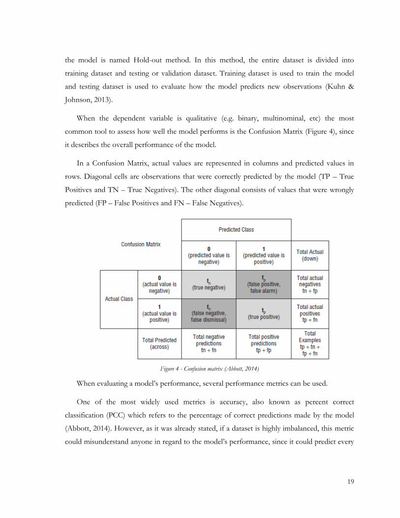
When the dependent variable is qualitative (e.g. binary, multinominal, etc) the most

common tool to assess how well the model performs is the Confusion Matrix (Figure 4), since

it describes the overall performance of the model.

In a Confusion Matrix, actual values are represented in columns and predicted values in

rows. Diagonal cells are observations that were correctly predicted by the model (TP – True

Positives and TN – True Negatives). The other diagonal consists of values that were wrongly

predicted (FP – False Positives and FN – False Negatives).

Figure 4 - Confusion matrix (Abbott, 2014)

When evaluating a model’s performance, several performance metrics can be used.

One of the most widely used metrics is accuracy, also known as percent correct

classification (PCC) which refers to the percentage of correct predictions made by the model

(Abbott, 2014). However, as it was already stated, if a dataset is highly imbalanced, this metric

could misunderstand anyone in regard to the model’s performance, since it could predict every

20

observation to belong to the majority class and still achieve a very high accuracy, nonetheless

(Kuhn & Johnson, 2013).

In an opposite way, error rate metric relates to the percentage of misclassified observations

made by the model (Kuhn & Johnson, 2013):

𝐸𝑟𝑟𝑜𝑟 𝑅𝑎𝑡𝑒 =𝑓𝑛 + 𝑓𝑝

𝑡𝑛 + 𝑡𝑝 + 𝑓𝑛 + 𝑓𝑝 (2.1)

Two alternative performance measures are sensitivity and specificity, both used in

classification problems. On one hand, sensitivity, also called as true positive rate, measures the

percentage of actual positives (true positives) that the model correctly predicted as such. On

the other hand, specificity, also named true negative rate, represents the percentage of actual

negatives (true negatives) that were correctly labeled by the model as such. These metrics can

be highly useful in certain cases, where predicting a specific class in a correct way is more

valuable than predicting correctly the other class (Kuhn & Johnson, 2013).

Two other measures are commonly used by practitioners and users of machine learning:

precision and recall. Precision consists on the percentage of predicted positives that were

correctly predicted as such by the model and recall is the same concept of sensitivity: actual

positive cases that were correctly predicted by the model (Abbott, 2014).

In some classification problems, it is important to take into account both precision and

recall metrics. In the presence of a problem where precision and recall are both relevant, there

is another performance metric that can be useful: F-score (also called F-measure). F-score is

the harmonic mean of precision and recall and, since it is not possible to maximize both

metrics at the same time, this metric can be quite useful in this kind of classification problem,

since by using this metric, one can select the best performing model that maximizes it. The F-

score is evenly balanced when β = 1 and favors precision when β > 1 and recall when β < 1. F-

Score is calculated by the following expression (adapted from Sokolova, Japkowicz, and

Szpakowicz (2006):

𝐹 − 𝑠𝑐𝑜𝑟𝑒 =

(𝛽2 + 1) × 𝑝𝑟𝑒𝑐𝑖𝑠𝑖𝑜𝑛 × 𝑟𝑒𝑐𝑎𝑙𝑙

𝛽2 × 𝑝𝑟𝑒𝑐𝑖𝑠𝑖𝑜𝑛 + 𝑟𝑒𝑐𝑎𝑙𝑙 (2.2)

21

Another common measure is the Receiver Operating Characteristic (ROC) curve (Figure

5). This graphical plot is created by plotting the true positive rate (sensitivity) against the false

positive rate (1 – specificity) along different thresholds (Kuhn & Johnson, 2013).

Figure 5 - An example of ROC curve (Kuhn & Johnson, 2013)

Another use of this chart is to calculate the area under the curve (AUC) metric. This metric

illustrates model’s ability to distinguish examples from different classes in a correct way. AUC

is equal to the area under the ROC curve and it can assume a value between 0 and 1. The

diagonal line between the extremes (coordinates (0,0) and (1,1)) represents a random model

with an AUC of 0.5 (Abbott, 2014). The higher the AUC value the better is the model’s

performance (Kuhn & Johnson, 2013).

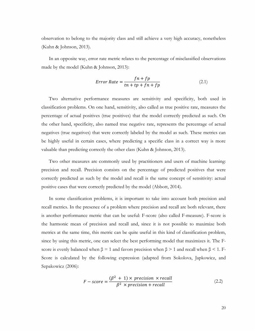
Figure 6 shows a summary of the concepts and formulas of the most used performance

metrics on a supervised classification problem.

22

Figure 6 - Performance measures (Abbott, 2014)

2.8. Similar studies

The existing academic works on predictive modelling applied to lead scoring are still

seldom or are based on custom algorithms and not on common tools used by data scientists

(Mortensen, Christison, Li, Zhu, & Venkatesan, 2019; Yan, Zhang, et al., 2015). Despite the

fact that the academic studies that used machine learning techniques applied to this specific

problem are not extensive, it was possible to find a handful of articles that address this

problem or similar problems as the topic under analysis.

Thus, the studies presented on the following paragraphs were quite relevant as they all

relate to the inherent purpose of the concept of lead scoring, in spite not being specifically

labeled as lead scoring studies.

23

Given the lack of research regarding predicting sales opportunity outcome, Mortensen et

al. (2019) provided an initial understanding of the concept and addressed some models to

classify and predict win propensities for sales opportunities. Particular attention was given to

this study since the data sourced for the project was extracted from a CRM platform (Salesforce),

similarly to the one that was used on this research. The purpose of the study was to identify

customers’ individual attributes that influence sales outcome, that is, what drives sales success

of a specific paper and packaging company and also to develop a machine learning model that

could predict sales success.

The authors address the problem of predicting sales success as a typical machine learning

binary classification problem. Thus, the authors used four supervised machine learning

algorithms suited to this problem: Multiple Logistic Regression (GLM), Decision Tree,

Random Forest and XGBoost. The performance metrics used to evaluate the models were the

following: accuracy, precision, variable importance and efficiency (resources used to build the

model). Out of the four models applied, Random Forest was the one that achieved better

performances in terms of accuracy but also regarding interpretation of what features influence

sales success the most, which proved to be an improvement comparing to the actual intuition

based system of sales forecast practiced by the company under study.

Chou, Grossman, Gunopulos, and Kamesam (2000) focused on the use of data mining

techniques to study the problem of selecting prospective customers from a large audience. The

study was carried out to an insurance company and authors purpose different approaches to

identify prospective customers (new households) when different types of data are available.

The study emphasizes the importance of understanding the characteristics of those who are

buying any type of product, since that insights allow the identification of prospective new

customers and target those who have the highest propensity to buy, hence increasing the odds

of a successful sale.

As the authors state, the ideal scenario for a problem like this one is when Client vs. Non

Client (or Buyer vs Non-Buyer) data is available, which is quite straightforward. However, the

authors defend that this type of data is expensive and in most of the cases not available,

affirming at the same time that companies do have extensive data regarding its customer base.

24

In spite the fact that this data does not directly provide information of who might be a client

and who might not, the authors state that this data still has useful insights to be extracted.

Hence, the authors applied an unsupervised learning technique (Clustering) when only data

about existing customers is available, by grouping them based on their characteristics. Once

the segments are defined, they are further analyzed and studied. Customer profiles are

designed, and these profiles are used to identify prospective customers.

When customer data and data for a set of market population are available, the authors

suggest the application of a supervised learning technique (Decision Tree) to develop a

customer prospecting strategy. Given data related to a set of customers and data of a sample of

market population, the authors suggest the application of a Decision Tree algorithm so that the

insurance company could then distinguish between prospects that are more likely to turn into

customers and prospects that do not. The company would then be able to score those

prospects and then target the ones that have the higher propensity to become customers, given

that score.

Duncan and Elkan (2015) published research within the topic of sales funnel predictive

analysis. Similarly to the study proceeded by Mortensen et al. (2019), the data used in the study

was extracted from a CRM platform, and included static features (also called demographic

features) and behavioral features (also called activity features). Demographic features relate to

information about the lead itself (industry, country, number of employees, market value,

among others). Behavioral features comprise aspects related to actions taken by the sales lead

and captured by the CRM platform that could denote about the interest of the lead in the

product/service. Examples of behavioral features include visits to the website and/or opening

a marketing email.

The main purpose of the research was to overcome the traditional lead scoring systems

used by both companies under study. According to the authors, as it was referred before,

manual lead scoring systems are hand-tuned and thus error-prone. The authors defend that

companies should then use a predictive model to prioritize sales leads, that is, to allocate

efforts and resources towards leads that are more likely to become a successful sale (customer).

25

Hence, machine learning models emerged to replace those intuition systems and bias

caused by them. The models developed by the authors, predicted not only the probability of a

lead to result in a successful sale (Won/Lost), but also the probability of reaching the next

stage of the sales funnel and also the expected revenue of any given lead.

Two methods were purposed for modeling prospective customers moving through a sales

funnel: DQM (Direct Qualification model) and FFM (Full Funnel Model).

DQM consists of predicting whether a lead will convert or not and it was approached by

the authors as a classification problem, replicating what was done in some previously

mentioned studies. Gradient Boosted Tree was the machine learning algorithm applied.

On the other hand, FFM consists of predicting whether a lead will advance through each

stage of the sales funnel or not, mainly from lead to SQL (Sales Qualified Lead) and from SQL

to successful sale (Won). The FFM was developed also to predict about the expected revenue

of a SQL. Gradient Boosted Tree was the machine learning algorithm applied.

An important conclusion drawn by this study is that the model performed well even when

activity data was excluded from the dataset, which means that high quality leads can be

identified even when only demographic features are available. Those methods result in an

increase of successful sales and total revenue and decrease of time to qualify leads, for both

companies under study.

Yan, Zhang, et al. (2015) published work regarding sales funnel win-propensity prediction

in a B2B scenario. The authors developed a model based on the two-dimensional Hawkes

process designed to estimate the lead-level win propensity within a certain time window. Its

goal is to update on a weekly basis the win likelihood of each sales-lead. This work is quite

interesting since the authors suggest a new approach that aimed to address the dynamic nature

of a sales pipeline activity: the interaction between salesperson and lead. Thus, the work has

been done not only to capture the static features of a sales pipeline, that is, the demographic

characteristics of sales-leads, but also to assess the activities between seller and lead, along the

sales life-cycle. The authors defend that this type of interactions carry a lot of valuable

information when predicting the outcome of a sales opportunity, since when analyzing the

sales pipeline of the company in question, a pattern emerged from the interaction between

26

salespersons and leads. The authors concluded that those interactions could trigger a successful

sale.

Although it is an interesting approach, the work relies too much on the presence (or

absence) of certain features (seller-lead interaction features) that most of the times are not

populated or updated by salesperson on the company’s CRM platform. As pointed out by

Duncan and Elkan (2015), in many companies, sales teams are overcrowded with sales-leads,

that is, have more leads than the ones that they can handle, which implies inaccuracies and

undisciplined activities regarding updating customer profiles on CRM platforms along the sales

life-cycle, which can affect the solution purposed by Yan, Zhang, et al. (2015).

Yan, Gong, Sun, Huang, and Chu (2015) also published research within the topic of win

propensity prediction. The authors, as many other academics, defend that this subject is the

foundation for resource optimization regarding sales pipeline management, which in turn,

when applied, increases lead’s conversion rates, and enables companies to reach their financial

goals. In this research, as in other academic published work, the problem is depicted as a

binary classification task. The authors suggest a logistic regression algorithm to be applied to

estimate the likelihood that sales opportunities have to become customers and gain score is

used as performance metric to evaluate the model for its interpretation power.

D’Haen and Van den Poel (2013) developed a quantitative model to support sales

representatives along the process of customer acquisition in a B2B scenario, in spite of the size

of the company or industry where it operates. However, the authors expect the model to be

highly efficient in highly saturated markets, where the customer acquisition process is costly, in

contrary to markets where are few players operating in it. The main objective of the model is

to predict sales outcome without human interference, thus it was developed to make the

customer acquisition process less intuition based. The authors defend that a model with high

predictive power regarding forecasting the right leads to pursue can enable companies to save

time and consequently money.

The model purposed by D’Haen and Van den Poel (2013) consists on a three phase

method for the customer acquisition process. On the first phase unsupervised learning

technique (Clustering) is applied to conduct a profiling model, according to the current

27

customer base. According to the authors this step carries valuable information because it

enables companies to fully understand who their customers are. The underlying idea of this

phase is that pursuing leads with similar profiles to the current customers increases the

probability of those same leads to become customers in the future. The technique used by the

authors to search for similar profiles of the current customer base is the nearest neighbor

algorithm, meaning that for each current customer, the model ranks the k-nearest leads. The

list of ranked leads can be based on a certain variable or threshold. In sumary, phase 1’s output

is a list of prospects ranked regarding their similarity relatively to the actual customer base.

Some prospects will be pursued by sales representatives, while others not.

The second phase of the model consists on a propensity approach by applying machine

learning algorithms such as decision tree, logistic regression and neural networks to adress if a

prospect should become a sales opportunity or not. The output of this phase is the predicted

probability of each prospect of resulting on a succesful sale.

The third and last phase of the purposed model is a combination of the previous phases,

the similarities of phase 1 and the probabilities of phase 2.

Nygård and Mezei (2020) published work demonstrates that it is possible to predict the

outcome of sales opportunity with the application of machine learning algorithms to perform

lead scoring. Furthermore, with data visualization tools the authors illustrate the insights that is

possible to gather through an automated lead scoring process.

The four machine learning algorithms selected by the authors were the following: Decision

Tree, Random Forest, Logistic Regression and Neural Networks, being the Random Forest the

best performing model.

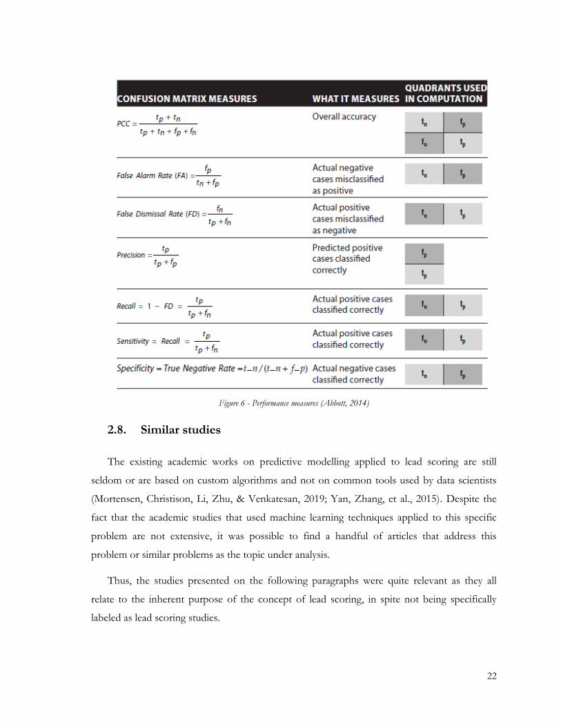
Table 1 provides a summary of the similar studies analysed regarding the topic of

predictive lead scoring under study.

28

Author Topic Algorithms

Mortensen et al. (2019)

Predicting sales outcome of sales opportunities

Supervised classification algorithms: Multiple Logistic

Regression (GLM), Decision Tree, Random Forest and XGBoost

Chou et al. (2000)

How to select and identify prospective customers from a large audience when different

types of data are available

Clustering technique when only data about existing customers is

available. Supervised learning technique

(Decision Tree) when customer data and data for a set of market

population are available

Duncan and Elkan (2015)

Research within the topic of sales funnel predictive analysis to

overcome the traditional lead scoring systems

Supervised classification algorithm: Gradient Boosted Tree

Yan, Zhang, et al. (2015)

Sales funnel win-propensity prediction in a business-to-

business (B2B) scenario within a forward time window

Two-dimensional Hawkes process model

Yan, Gong, et al. (2015)

Sales win propensity prediction Supervised classification algorithm:

Logistic regression

D’Haen and Van den Poel (2013)

Three phase quantitative method to support the customer

acquisition process and to predict sales outcome

Combination of unsupervised (Clustering k-nearest neighbor

algorithm) and supervised algorithms (Decision Tree,

Logistic Regression and Neural Networks)

Nygård and Mezei (2020)

An experimental case study in regard to automated lead scoring

Supervised learning algorithms: Decision Tree, Random Forest, Logistic Regression and Neural

Networks

Table 1 - Summary of similar studies regarding the topic of predictive lead scoring

29

3. Methodological Aspects

Along this chapter the suitable methodology regarding this internship report will be

discussed. In this report, a quantitative methodology was applied due to the nature of the

research topic.

HUUB’s main goal with this project is to increase conversion rates and improve sales

team’s performance.

Regarding this project itself, the main goal is to develop a lead scoring system in order to

contribute to HUUB’s goal stated above.

To improve HUUB’s sales team efficiency and optimization of resources, this project

consisted in developing a machine learning assisted lead scoring system. This system was

treated as a supervised learning classification problem thus, a machine learning algorithm that

predicts if a lead is classified as Won or Lost, taking into account lead’s demographical

characteristics (historical data), was developed. The confidence of that prediction should be

depicted as the criteria to decide which leads HUUB’s sales team should contact firstly. Leads

will be ranked according to the assigned score, meaning that top leads with higher scores

represent leads that have higher probability of resulting in successful sales.

In addition, a manual lead scoring system (lead scoring scorecard) is also going to be

presented and suggested to implement into the company under analysis CRM platform. The

lead scorecard was designed after an analysis of historical data extracted from the company

CRM platform.

Based on the similar studies discussed on previous section, and as this project in specific

requires, a CRISP-DM framework was adopted (Wirth & Hipp, 2000). CRISP-DM framework

is broken down in 6 steps, as following:

- Business understanding (this first step focuses on understanding what are the desired

business outputs of the project);

- Data understanding (this phase focuses on collecting the data necessary for the project

as well as doing a data exploration report);

30

- Data preparation (this step covers all the activities regarding the preparation of the data

set to develop the model. It includes the elaboration of a data cleaning report, if

necessary);

- Modelling (in this stage, modeling techniques are selected and applied);

- Evaluation (performance metrics are analyzed to ascertain model’s performance);

- Deployment

3.1. Phases/Steps of the study

In the diagram below, the different phases/steps that this project considered to pursue the

main research topic are presented. Business Understanding was the first step followed by Data

Understanding and Data Preparation. Then, the more technical part of this project was

initiated: Modelling followed by the appropriate Evaluation of the models’ performance.

Figure 7 - CRISP-DM Process Model for Data Mining projects (Wirth & Hipp, 2000)

31

The software tool used in this study was RapidMiner. RapidMiner is a data science

platform, used for data preparation, machine learning, deep learning, text mining and

predictive analytics (Gulia, 2016).

32

4. Empirical study

This chapter addresses the details of this project. Section 4.1 refers to the first step of the

study that is to discuss the business problem in analysis. Section 4.2 relates to data

understanding and the process of data extraction, exploration and description. On section 4.3

the process of data preparation is addressed, namely data cleaning and data transformation.

Section 4.4 relates to the modelling part of this project addresses the process of building the

model. On section 4.5 the framework used to validate models’ performance is described.

4.1. Business Understanding

HUUB aims to implement a sales machine, focused on five vectors: process, automation,

analytics, platform and methodology. This sales machine urges to be implemented since a

solution is needed to support HUUB’s growth.

HUUB works with Hubspot, an all-in-one CRM platform that offers functionalities to

cover areas such as inbound marketing, services and sales (Hubspot, 2020). It is through this

platform that HUUB’s sales team manages and controls its entire sales pipeline and marketing

and sales activity.

The first step of this sales machine relates to lead generation. HUUB’s lead generation is

done through 2 strategies: inbound strategy and outbound strategy. HUUB’s inbound strategy

lives by growth hacking, organic reach and brand awareness. It includes fashion brands that are

interested in HUUB’s services and because of that reach HUUB to establish a partnership

between both parts. Outbound strategy relates to contact fashion brands and to promote

HUUB’s product and value proposition directly to them.

As it was discussed on the literature review section (see section 2.3), in spite of the

common structure of any company’s sales funnel, every organization designs its sales funnel in

a specific way, suited to its customer acquisition process. Thus, it is relevant to detail more

information about HUUB’s sales pipeline, to provide a more clear understanding of the sales

machine that HUUB aims to implement. Figure 8 provides a schematic and simple view of

HUUB sales pipeline.

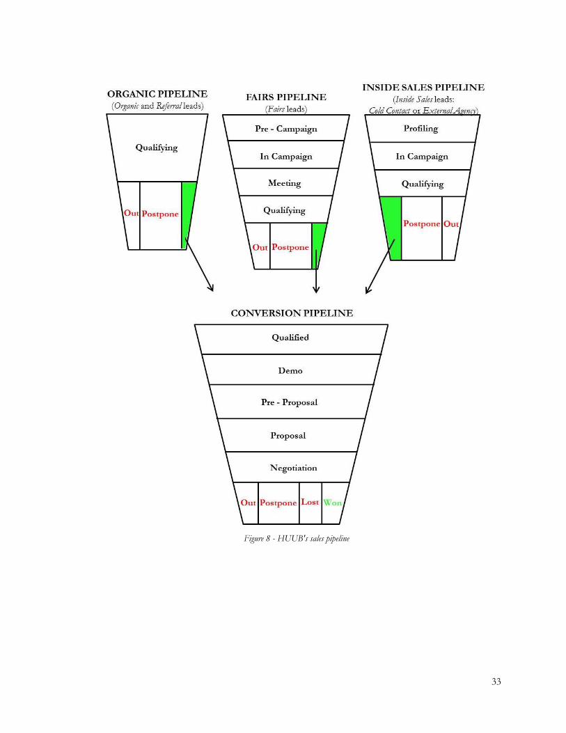
33

Figure 8 - HUUB's sales pipeline

34

Regarding HUUB’s sales pipeline, leads can be classified accordingly to its origin/source

and then allocated to a specific sub-pipeline.

In regard to inbound strategy, leads that contact HUUB directly to know more about its

services are classified as Organic leads (Organic Pipeline). Fashion brands can also contact HUUB

through a referral provided from an actual customer (Referral leads). In both cases, HUUB did

not spend any direct effort with them.

On the other hand, regarding outbound strategy, leads can assume two categories: Fairs

leads (leads generated through tradeshows’ visits and allocated to Fairs Pipeline) or Inside Sales

leads, allocated to Inside Sales Pipeline.

Most of HUUB’s leads are generated through offline sources. Leads can be either

generated through a partnership established with an external marketing agency, dedicated to

deliver 500 new leads to be contacted every month or through an intern profiling (Cold

Contact), that is, through an investigation and search pursued by HUUB’s sales personnel, with

the objective of collecting new prospects to be contacted, with the long-term objective of

becoming future HUUB’s clients.

After being allocated to a predefined sub-pipeline (Organic Pipeline, Fairs Pipeline or Inside

Sales Pipeline) the path and stages that any lead follows depend on the predefined sub-pipeline

where it was allocated.

Regarding leads generated through Inside Sales strategy, the process of converting a lead

into a client starts when an email is sent to the brand. 120 new brands are contacted every

month by HUUB’s sales team. A lead goes through the following stages on this pipeline (Inside

Sales Pipeline):

- Profiling: relates to obtaining information about certain characteristics of the fashion

brand: Email, Brand Type, Product Category, Country, Production, among others;

- In Campaign: represents the moment when an email is sent to the brand. This email can

be sent to a general email or to a personal email, depending on the contact that was possible to

gather. The brand awaits on this pipeline until an answer is provided;

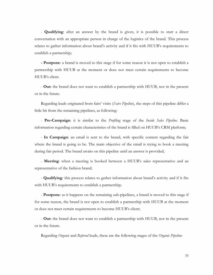
35

- Qualifying: after an answer by the brand is given, it is possible to start a direct

conversation with an appropriate person in charge of the logistics of the brand. This process

relates to gather information about brand’s activity and if it fits with HUUB’s requirements to

establish a partnership;

- Postpone: a brand is moved to this stage if for some reason it is not open to establish a

partnership with HUUB at the moment or does not meet certain requirements to become

HUUB’s client.

- Out: the brand does not want to establish a partnership with HUUB, nor in the present

or in the future.

Regarding leads originated from fairs’ visits (Fairs Pipeline), the steps of this pipeline differ a

little bit from the remaining pipelines, as following:

- Pre-Campaign: it is similar to the Profiling stage of the Inside Sales Pipeline. Basic

information regarding certain characteristics of the brand is filled on HUUB’s CRM platform;

- In Campaign: an email is sent to the brand, with specific content regarding the fair

where the brand is going to be. The main objective of the email is trying to book a meeting

during fair period. The brand awaits on this pipeline until an answer is provided;

- Meeting: when a meeting is booked between a HUUB’s sales representative and an

representative of the fashion brand;

- Qualifying: this process relates to gather information about brand’s activity and if it fits

with HUUB’s requirements to establish a partnership;

- Postpone: as it happens on the remaining sub-pipelines, a brand is moved to this stage if

for some reason, the brand is not open to establish a partnership with HUUB at the moment

or does not meet certain requirements to become HUUB’s client;

- Out: the brand does not want to establish a partnership with HUUB, nor in the present

or in the future.

Regarding Organic and Referral leads, these are the following stages of the Organic Pipeline:

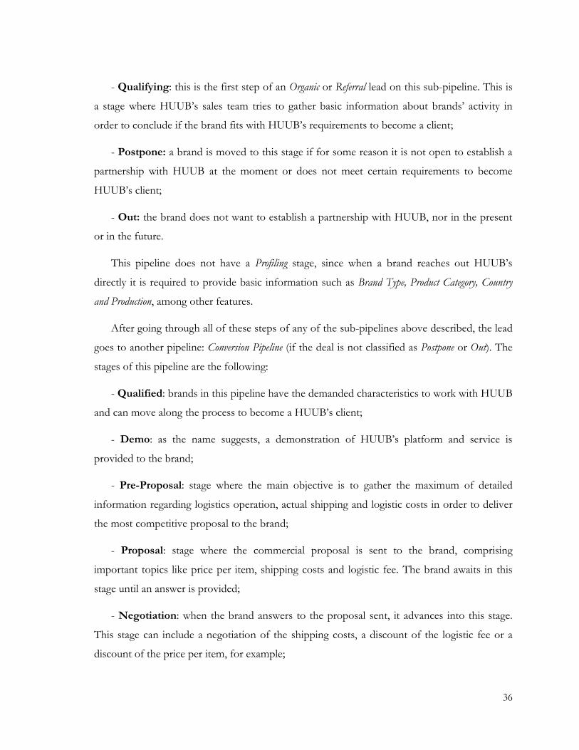
36

- Qualifying: this is the first step of an Organic or Referral lead on this sub-pipeline. This is

a stage where HUUB’s sales team tries to gather basic information about brands’ activity in

order to conclude if the brand fits with HUUB’s requirements to become a client;

- Postpone: a brand is moved to this stage if for some reason it is not open to establish a

partnership with HUUB at the moment or does not meet certain requirements to become

HUUB’s client;

- Out: the brand does not want to establish a partnership with HUUB, nor in the present

or in the future.

This pipeline does not have a Profiling stage, since when a brand reaches out HUUB’s

directly it is required to provide basic information such as Brand Type, Product Category, Country

and Production, among other features.

After going through all of these steps of any of the sub-pipelines above described, the lead

goes to another pipeline: Conversion Pipeline (if the deal is not classified as Postpone or Out). The

stages of this pipeline are the following:

- Qualified: brands in this pipeline have the demanded characteristics to work with HUUB

and can move along the process to become a HUUB’s client;

- Demo: as the name suggests, a demonstration of HUUB’s platform and service is

provided to the brand;

- Pre-Proposal: stage where the main objective is to gather the maximum of detailed

information regarding logistics operation, actual shipping and logistic costs in order to deliver

the most competitive proposal to the brand;

- Proposal: stage where the commercial proposal is sent to the brand, comprising

important topics like price per item, shipping costs and logistic fee. The brand awaits in this

stage until an answer is provided;

- Negotiation: when the brand answers to the proposal sent, it advances into this stage.

This stage can include a negotiation of the shipping costs, a discount of the logistic fee or a

discount of the price per item, for example;

37

- Won: when the brand becomes HUUB’s client and the partnership is established;

- Postpone: if for some reason, the brand is not open to establish a partnership with

HUUB at the moment, but does not close the opportunity to become HUUB’s client in the

future;

- Lost: there is no possibility for the brand to become a HUUB’s client in the present

moment, due to some reason.

After being classified as Won (successful sale), new clients go along to the final pipeline of

the sales process: Onboarding Pipeline. This is the prior stage where details and specificities

regarding the logistic operation are defined before the entire process is classified as done.

Then, the activity between HUUB and the fashion brand is finally initiated.

Given this context information regarding HUUB’s sales pipeline and HUUB’s exponential

growth, and as the number of leads increase along time, a criteria needs to be defined in order

to know which leads should be contacted in the first place, otherwise HUUB’s sales team will

not be the most efficient possible. HUUB has got more than 800 leads on its sales pipeline that

were not contacted yet and, as it was referred before, this number increases on a daily basis,

through online and offline sources. Besides that, HUUB has approximately 1300 active leads,

that is, leads with open sales processes.

At the moment, HUUB’s criteria of which lead to contact firstly is almost an ad-hoc

process. This means that the sales team might not be targeting the best leads, that is, leads that

have a higher propensity of resulting in successful sales.

Yet, active leads with open sales processes might receive different attention and effort by

sales personnel given its probability of resulting in a successful sale.

Given that, the project of developing a lead scoring system to HUUB reveals to be a

crucial priority to this company in order to promote its sales department efficiency and to

pursue long-term growth for the organization.

38

4.2. Data Understanding

In this section, the content of the dataset extracted from HUUB’s CRM platform

containing information about HUUB’s leads is analysed. Potential problems are monitored and

further corrected.

4.2.1. General Overview

Historical data was extracted from HUUB’s CRM platform and contains 5977 entities

(fashion brands), each one with 76 features.

At the very beginning of this step, some data quality issues emerged as the data was not

fulfilled correctly and some features had too many typing errors among the enormous range of

possible values. So, it was clear that an initial data preparation was necessary before going

further in the process.

Regarding the dataset, most of the features are categorical variables; thus the following

descriptive statistical analysis consists of plotting the histogram of each feature and analysing

the frequencies and mode of each one, since common statistical measures were not possible to

calculate, such as mean, median or mode. Also, it was important to assure that every value was

written in a uniformed way, so that an appropriate data analysis could be made. As an example,

regarding the feature Production, there were brands that had the value UK and other brands that

had the value United Kingdom, which in fact relates to the same exact country. This is just an

example of some of the data quality issues that emerged in a first moment. These same issues

were corrected and exploratory data analysis was then processed. This step was fundamental to

pursue the overall objective of the project. However, it is important to note that the main

purpose of the data preparation done at this stage was to make the data understanding step

doable and not to prepare the data to the modelling step, although it is intrinsic to that step. In

some data mining projects, data preparation is made along the entire project, thus, an initial

data preparation was made at the very beginning of this project.

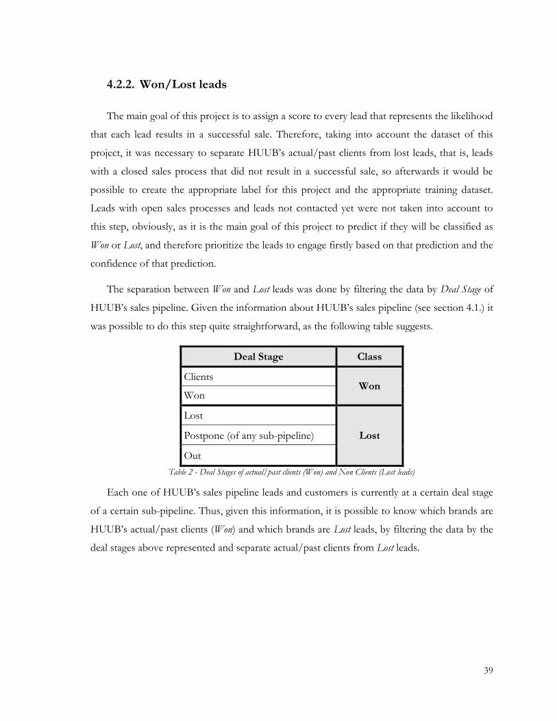
39

4.2.2. Won/Lost leads

The main goal of this project is to assign a score to every lead that represents the likelihood

that each lead results in a successful sale. Therefore, taking into account the dataset of this

project, it was necessary to separate HUUB’s actual/past clients from lost leads, that is, leads

with a closed sales process that did not result in a successful sale, so afterwards it would be

possible to create the appropriate label for this project and the appropriate training dataset.

Leads with open sales processes and leads not contacted yet were not taken into account to

this step, obviously, as it is the main goal of this project to predict if they will be classified as

Won or Lost, and therefore prioritize the leads to engage firstly based on that prediction and the

confidence of that prediction.

The separation between Won and Lost leads was done by filtering the data by Deal Stage of

HUUB’s sales pipeline. Given the information about HUUB’s sales pipeline (see section 4.1.) it

was possible to do this step quite straightforward, as the following table suggests.

Deal Stage Class

Clients Won

Won

Lost

Lost Postpone (of any sub-pipeline)

Out

Table 2 - Deal Stages of actual/past clients (Won) and Non Clients (Lost leads)

Each one of HUUB’s sales pipeline leads and customers is currently at a certain deal stage

of a certain sub-pipeline. Thus, given this information, it is possible to know which brands are

HUUB’s actual/past clients (Won) and which brands are Lost leads, by filtering the data by the

deal stages above represented and separate actual/past clients from Lost leads.

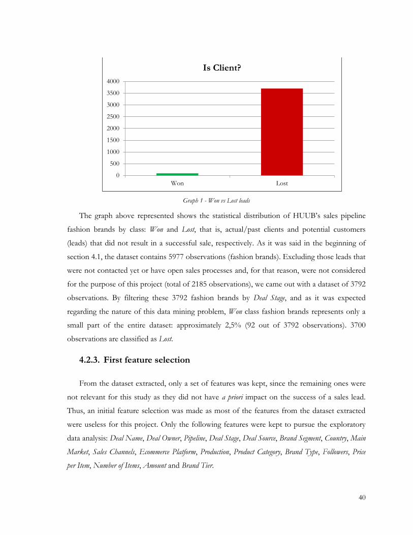
40

Graph 1 - Won vs Lost leads

The graph above represented shows the statistical distribution of HUUB’s sales pipeline

fashion brands by class: Won and Lost, that is, actual/past clients and potential customers

(leads) that did not result in a successful sale, respectively. As it was said in the beginning of

section 4.1, the dataset contains 5977 observations (fashion brands). Excluding those leads that

were not contacted yet or have open sales processes and, for that reason, were not considered

for the purpose of this project (total of 2185 observations), we came out with a dataset of 3792

observations. By filtering these 3792 fashion brands by Deal Stage, and as it was expected

regarding the nature of this data mining problem, Won class fashion brands represents only a

small part of the entire dataset: approximately 2,5% (92 out of 3792 observations). 3700

observations are classified as Lost.

4.2.3. First feature selection

From the dataset extracted, only a set of features was kept, since the remaining ones were

not relevant for this study as they did not have a priori impact on the success of a sales lead.

Thus, an initial feature selection was made as most of the features from the dataset extracted

were useless for this project. Only the following features were kept to pursue the exploratory

data analysis: Deal Name, Deal Owner, Pipeline, Deal Stage, Deal Source, Brand Segment, Country, Main

Market, Sales Channels, Ecommerce Platform, Production, Product Category, Brand Type, Followers, Price

per Item, Number of Items, Amount and Brand Tier.

0

500

1000

1500

2000

2500

3000

3500

4000

Won Lost

Is Client?

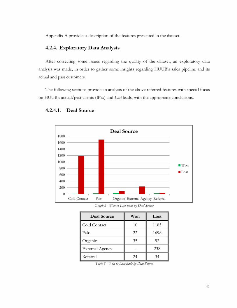
41

Appendix A provides a description of the features presented in the dataset.

4.2.4. Exploratory Data Analysis

After correcting some issues regarding the quality of the dataset, an exploratory data

analysis was made, in order to gather some insights regarding HUUB’s sales pipeline and its

actual and past customers.

The following sections provide an analysis of the above referred features with special focus

on HUUB’s actual/past clients (Won) and Lost leads, with the appropriate conclusions.

4.2.4.1. Deal Source

Graph 2 - Won vs Lost leads by Deal Source

Deal Source Won Lost

Cold Contact 10 1185

Fair 22 1698

Organic 35 92

External Agency - 238

Referral 24 34

Table 3 - Won vs Lost leads by Deal Source

0

200

400

600

800

1000

1200

1400

1600

1800

Cold Contact Fair Organic External Agency Referral

Deal Source

Won

Lost

42

Starting by analysing this feature, regarding HUUB’s actual and past clients it is clear that

more than 50% of these came from Organic source and Referrals. 1 actual/past client and 453

Lost leads do not have information regarding this feature and (missing values). There is a

discrepancy when a comparison is made between the Deal Source of unsuccessful sales (Lost),

and HUUB’s actual/past clients, as most of Lost leads on HUUB’s sales pipeline are generated

from tradeshows (Fair) or through intern profiling (Cold Contact).

It is possible to conclude that it tends to be easier for HUUB to turn leads into customers

that come from Organic source or Referral, which seems quite logic given what was referred on

section 4.1. Any lead that came through the External Agency is yet to be converted.

4.2.4.2. Brand Segment

Graph 3 - Won vs Lost leads by Brand Segment

Brand Segment Won Lost

Low Cost - 6

Luxury 2 127

Premium 78 1112

Premium; Value 1 2

Value 9 519

Table 4 - Won vs Lost leads by Brand Segment

0

200

400

600

800

1000

1200

Low Cost Luxury Premium Premium;Value

Value

Brand Segment

Won

Lost

43

Regarding the feature Brand Segment, 78 HUUB’s actual or past customers position itself as

Premium fashion brands. 9 describe itself as Value fashion brands, 2 as Luxury brands and 1 as

both Premium and Value brands. 2 actual/past customers do not present information regarding

its Brand Segment (missing values) and any Low Cost brand is still yet to be converted as a

customer. 1934 Lost leads do not have this feature populated. The tendency described before

regarding HUUB’s actual/past clients is still reflected on HUUB’s Lost leads, as Graph 3 and

Table 4 suggest. With this information, it is possible to conclude that HUUB sales strategy is

clearly aimed to target Premium fashion brands given the predominance on actual/past clients

but also on Lost leads of this type of fashion brands.

4.2.4.3. Country

Graph 4 - HUUB's actual/past clients by Country

This feature relates to the country of origin of the fashion brand. Thus, given the nature of

this feature, a lot of different values are expected. Among HUUB’s sales pipeline, there are

fashion brands from a range of 92 different countries. However, some countries are highly

represented, whether on HUUB’ actual/past clients or Lost leads.

When an analysis of HUUB’s actual/past clients is done, it is possible to conclude that

most of HUUB’s actual/past clients are Portuguese brands, as it is suggested by Graph 4

0

5

10

15

20

25

30

35

HUUB's actual/past clients by Country

44

above represented. 32 out of 92 clients are Portuguese, which can be explained since HUUB is

a Portuguese startup and has a warehouse in Portugal and, due to this fact, Portuguese brands

are more aware of HUUB’s value proposition. This conclusion suggests that HUUB tends to

have an advantage when trying to convert a Portuguese lead into a customer. Besides

Portuguese fashion brands, HUUB’s client portfolio is mainly composed by European brands,

as 56 out of 92 clients are from the European continent. Thus, 88 brands are European brands

(56 from different European countries plus 32 Portuguese fashion brands) which enhance the

predominance of clients from the European continent on HUUB’s customer portfolio. The

remaining 3 customers are from the USA. 1 actual/past client does not have this feature

populated.

Regarding Lost leads, the range of countries is broader, as it was expected given the higher

number of Lost leads, hence the expanded range of countries. However, it is still possible to

observe a tendency similar to what was described about actual/past clients.

European leads are also the majority of Lost leads, with specific relevance of Spanish,

French, Italian, Britain, German, Danish and Dutch leads. An aspect that stands out is the fact

that there are a significant number of Italian Lost leads despite the fact that HUUB does not

have any Italian fashion brand on its portfolio. 85 Lost leads do not have this feature

populated.

4.2.4.4. Main Market(s)

Given the concept of this feature, as it occurred with the feature Country it is also expected

that it presents a wide variety of values. HUUB’s sales pipeline contains 44 different values

regarding Main Market(s) feature. However, some conclusions can be drawn, as Graph 5 and

Table 5 suggest. It is important to note that regarding the nature of this feature, many leads do

not have information about its Main Market(s), as this information is only provided on an

advanced stage of the sales lifecycle. Yet, it is relevant to state that any fashion brand can have

more than 1 main market.

45

Graph 5 - Won vs Lost leads by Main Market(s)

Main Market(s) Won Lost

Europe 77 611

North America 14 75

Central & South America 1 -

Asia 10 46

Africa & ROW 1 3

Middle East 4 20

Table 5 - Won vs Lost leads by Main Market(s)

Regarding HUUB’s actual/past customers, Europe and/or European countries have

preponderance as values of the Main Market(s) feature. 77 out of 92 brands have Europe as a

main market or one of many main markets or a European country as its only main market. 9

customers do not have this feature populated.

This tendency is also observed when analysing Lost leads as 611 leads have the European

continent or a European country as its main market or as one of its main market. 3066 Lost

leads do not have this feature populated. Given the location of HUUB’s warehouses (Portugal

and Netherlands) it is understandable that HUUB tends to find easier to convert into

customers leads that have the European continent or a European country as main market,

rather than brands that have positioned themselves in the Asian or American continent, for

example.

0

100

200

300

400

500

600

700

Europe NorthAmerica

Central &South

America

Asia Africa &ROW

MiddleEast

Main Market(s)

Won

Lost

46

4.2.4.5. Sales Channel(s)

Any fashion brand can operate through one (or many) of the following sales channels:

Ecommerce, Marketplace, Own Stores and Wholesale.

Graph 6 - Won vs Lost leads by Sales Channel(s)

Sales Channel(s) Won Lost

Ecommerce 85 2078

Wholesale 57 2543

Own Stores 6 426

Marketplace 2 83

Table 6 - Won vs Lost leads by Sales Channel(s)

As it was expected, the majority of HUUB’s customer portfolio sells its products through

online channels (Ecommerce) or through Wholesale channels. Brands that sell its products

through Marketplace and/or Own Stores represent a minor part of HUUB’s actual/past

customers. 1 actual/past client does not have this feature fulfilled.

Analysing HUUB’s Lost leads there is a tendency of unsuccessful sales towards brands that

have Wholesale as its major sales channel, as shown on Table 6 and Graph 6 above represented.

233 Lost leads do not have this feature populated.

0

500

1000

1500

2000

2500

3000

Ecommerce Wholesale Own Stores Marketplace

Sales Channel(s)

Won

Lost

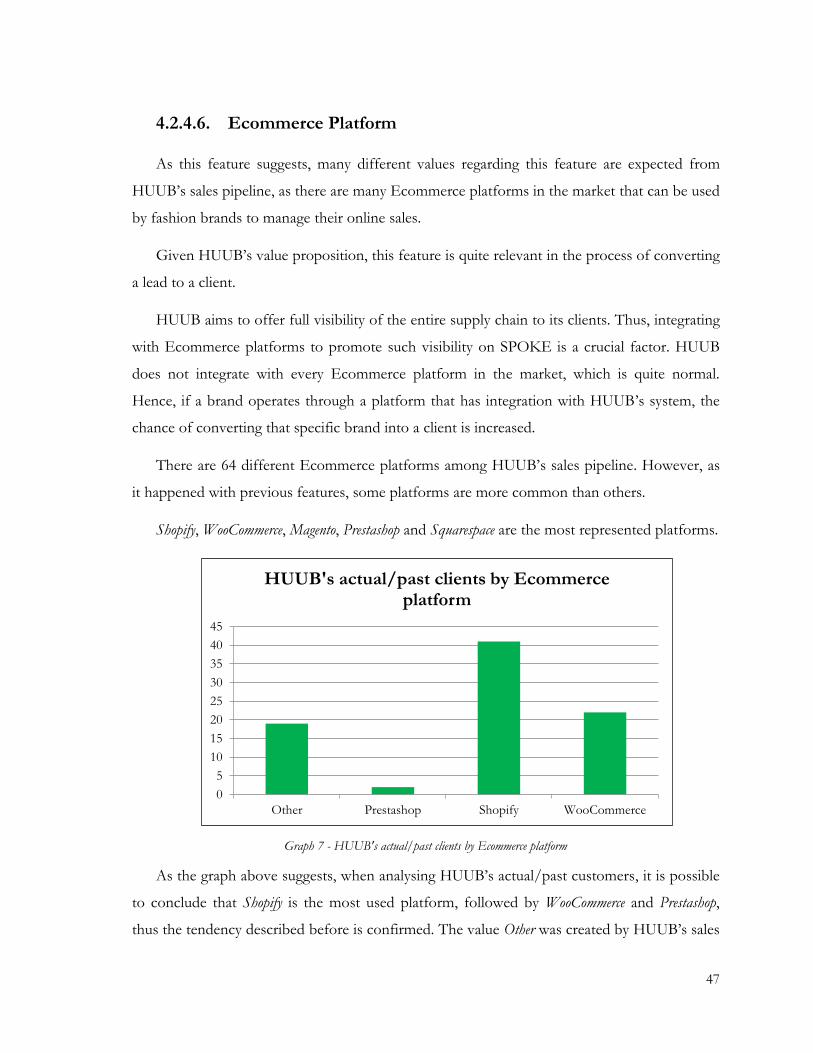
47

4.2.4.6. Ecommerce Platform

As this feature suggests, many different values regarding this feature are expected from

HUUB’s sales pipeline, as there are many Ecommerce platforms in the market that can be used

by fashion brands to manage their online sales.

Given HUUB’s value proposition, this feature is quite relevant in the process of converting

a lead to a client.

HUUB aims to offer full visibility of the entire supply chain to its clients. Thus, integrating

with Ecommerce platforms to promote such visibility on SPOKE is a crucial factor. HUUB

does not integrate with every Ecommerce platform in the market, which is quite normal.

Hence, if a brand operates through a platform that has integration with HUUB’s system, the

chance of converting that specific brand into a client is increased.

There are 64 different Ecommerce platforms among HUUB’s sales pipeline. However, as

it happened with previous features, some platforms are more common than others.

Shopify, WooCommerce, Magento, Prestashop and Squarespace are the most represented platforms.

Graph 7 - HUUB's actual/past clients by Ecommerce platform

As the graph above suggests, when analysing HUUB’s actual/past customers, it is possible

to conclude that Shopify is the most used platform, followed by WooCommerce and Prestashop,

thus the tendency described before is confirmed. The value Other was created by HUUB’s sales

0

5

10

15

20

25

30

35

40

45

Other Prestashop Shopify WooCommerce

HUUB's actual/past clients by Ecommerce platform

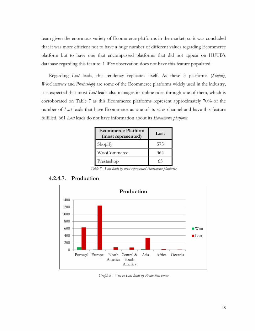
48

team given the enormous variety of Ecommerce platforms in the market, so it was concluded

that it was more efficient not to have a huge number of different values regarding Ecommerce

platform but to have one that encompassed platforms that did not appear on HUUB’s

database regarding this feature. 1 Won observation does not have this feature populated.

Regarding Lost leads, this tendency replicates itself. As these 3 platforms (Shopify,

WooCommerce and Prestashop) are some of the Ecommerce platforms widely used in the industry,

it is expected that most Lost leads also manages its online sales through one of them, which is

corroborated on Table 7 as this Ecommerce platforms represent approximately 70% of the

number of Lost leads that have Ecommerce as one of its sales channel and have this feature

fulfilled. 661 Lost leads do not have information about its Ecommerce platform.

Ecommerce Platform (most represented)

Lost

Shopify 575

WooCommerce 364

Prestashop 65

Table 7 - Lost leads by most represented Ecommerce platforms

4.2.4.7. Production

Graph 8 - Won vs Lost leads by Production venue

0

200

400

600

800

1000

1200

1400

Portugal Europe NorthAmerica

Central &South

America

Asia Africa Oceania

Production

Won

Lost

49

Production Won Lost

Portugal 74 630

Europe 11 1243

North America - 70

Central & South America 1 66

Asia 19 338

Africa 1 21

Oceania - 9

Table 8 - Won vs Lost leads by Production venue

HUUB’s sales pipeline presents a huge variety of values regarding this feature. Yet, it is

important to refer that leads can have its production in more than one location. However,

some patterns emerged.

It is easy to conclude that Portugal is the most represented production’s country and a

priority to HUUB’s sales strategy. In fact, given HUUB’s warehouse location, brands that have

its production in Portugal tend to be an easier target, since all the logistic costs reduce, given

the location and distance between production and logistic centers. This fact is represented on

Table 8 and Graph 8, as 74 out of 92 Won brands have one of its production centre located in

Portugal. The Asian and European continents are the remaining most common production

locations among HUUB’s actual/past clients. Leads with production in North America and in

Oceania are yet to be converted into a customer. 2 actual/past clients do not present

information about this feature. Regarding Lost leads, this tendency is also verified, with leads

with production in Portugal and/or in the European continent to be the most represented

ones. 1505 leads do not have this feature populated.

4.2.4.8. Product category

Any fashion brand can commercialize products of one or more than one of the following

categories: Apparel, Footwear, Accessories, Homewear, Swimwear, Underwear and/or Other.

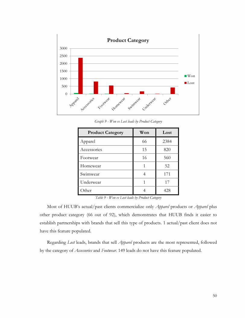
50

Graph 9 - Won vs Lost leads by Product Category

Product Category Won Lost

Apparel 66 2384

Accessories 15 820

Footwear 16 560

Homewear 1 52

Swimwear 4 171

Underwear 1 17

Other 4 428

Table 9 - Won vs Lost leads by Product Category

Most of HUUB’s actual/past clients commercialize only Apparel products or Apparel plus

other product category (66 out of 92), which demonstrates that HUUB finds it easier to

establish partnerships with brands that sell this type of products. 1 actual/past client does not

have this feature populated.

Regarding Lost leads, brands that sell Apparel products are the most represented, followed

by the category of Accessories and Footwear. 149 leads do not have this feature populated.

0

500

1000

1500

2000

2500

3000

Product Category

Won

Lost

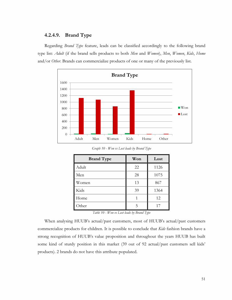
51

4.2.4.9. Brand Type

Regarding Brand Type feature, leads can be classified accordingly to the following brand

type list: Adult (if the brand sells products to both Men and Women), Men, Women, Kids, Home

and/or Other. Brands can commercialize products of one or many of the previously list.

Graph 10 - Won vs Lost leads by Brand Type

Brand Type Won Lost

Adult 22 1126

Men 28 1075

Women 13 867

Kids 39 1364

Home 1 12

Other 5 17

Table 10 - Won vs Lost leads by Brand Type

When analysing HUUB’s actual/past customers, most of HUUB’s actual/past customers

commercialize products for children. It is possible to conclude that Kids fashion brands have a

strong recognition of HUUB’s value proposition and throughout the years HUUB has built

some kind of sturdy position in this market (39 out of 92 actual/past customers sell kids’

products). 2 brands do not have this attribute populated.

0

200

400

600

800

1000

1200

1400

1600

Adult Men Women Kids Home Other

Brand Type

Won

Lost

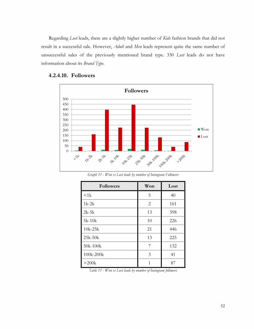
52

Regarding Lost leads, there are a slightly higher number of Kids fashion brands that did not

result in a successful sale. However, Adult and Men leads represent quite the same number of

unsuccessful sales of the previously mentioned brand type. 330 Lost leads do not have

information about its Brand Type.

4.2.4.10. Followers

Graph 11 - Won vs Lost leads by number of Instagram Followers

Followers Won Lost

<1k 5 40

1k-2k 2 161

2k-5k 13 398

5k-10k 10 226

10k-25k 21 446

25k-50k 13 225

50k-100k 7 132

100k-200k 3 41

>200k 1 87

Table 11 - Won vs Lost leads by number of Instagram followers

0

50

100

150

200

250

300

350

400

450

500

Followers

Won

Lost

53

This feature relates to the number of followers of the fashion brand’s Instagram profile.

Number of followers were allocated to predefined followers classes in order to pursue a more

easily and understandable interpretation, as Graph 11 and Table 11 represent.

HUUB’s successful sales along the years demonstrate that most of them have an Instagram

page with 10k to 25k followers. Regarding actual/past clients, 17 do not have information

about Instagram followers.

Lost leads describe the same tendency being the class of 2k-5k Instagram followers the

following most represented class. 1944 Lost leads do not have information about the number

of Instagram followers, whether the brand does not have an Instagram profile or simply because

this feature is not populated.

4.2.4.11. Number of items

Fashion industry is often classified in 2 seasons (Autumn/Winter and Spring/Summer).

This feature relates to the expected number of items that a fashion brand aims to

commercialize in a season (half a year). As a lead advances through the stages of the sales

pipeline, more information is provided to HUUB’s sales representatives and is entered in the

CRM platform. Yet, certain information is only gathered on an advanced stage of the sales

cycle, which is easy to comprehend. Leads with no interest on establishing a partnership with

HUUB obviously do not reach a stage where exchange information about its commercial

activity and numbers, but a fashion brand that is on the final stages of the sales pipeline, is

often asked to provided information of this nature.

Therefore, a high number of missing values of this features is expected, namely on Lost

leads, which is corroborated as the number of Lost leads that do not have this feature

populated ascends to 3020. Yet, 2 HUUB’s actual/past clients also do not have information

about this feature.

4.2.4.12. Price per Item

Before analysing this feature it is important to refer that regarding the concept of it, this

feature is only populated in an advanced stage of the sales cycle, that is, when a proposal is

54

sent to the fashion brand. Hence, the number of leads (Lost and Active leads) of HUUB’s sales

pipeline that do not have information about this feature is significant (5569 leads).

In regard to HUUB’s actual/past customers, each one has information about its feature.

This fact is not verified by Lost leads, as expected. Only 229 out of 3700 leads had a price per

item assigned before resulting in an unsuccessful sale.

Graph 12 - Won vs Lost leads by Price per Item

Price per Item Won Lost

<= 0,75€ 7 3

]0,75€ - 1€[ 34 20

>= 1€ 51 206

Table 12 - Won vs Lost leads by Price per Item

Different values of prices per item were aggregated into three classes to pursue the analysis

of this feature: >=0,75€, ]0,75€ - 1€[ and >=1€.

It is clear that most of Won and Lost leads have a price per item equal or higher than 1,00€.

51 actual/past clients pay/paid a price per item equal or higher than 1,00€.

This feature is not quite relevant regarding Lost leads as it is only filled in in an advanced

stage of the sales cycle. Plus, data suggests that most leads result in an unsuccessful sale prior

0

50

100

150

200

250

<= 0,75€ ]0,75€ - 1€[ >= 1€

Price per Item

Won

Lost

55

to the moment when a proposal is sent to the brand, as the number of missing values of this

feature is significant (3471 leads do not have this feature populated).

4.2.4.13. Amount (ARR)

ARR (Annual Recurrent Revenue) is an essential metric for SaaS (Software as a Service)

businesses, which is what HUUB is trying to become. It is a proxy of how much year on year

revenue a company can expect, based on yearly subscriptions. In HUUB’s business model,

ARR is calculated through the following formulas, depending on what is the sales channel of

the brand:

ARR (Ecommerce): number of items per season x price per item x 3

ARR (Wholesale): number of items per season x price per item x 2

As the following feature (Brand Tier) is correlated with this one and, due to that, allows

drawing the same conclusions as this one, the major topic to discuss about this feature relates

to the pattern that emerged among the possible values for this feature, namely when analysing

Lost leads. This fact was not verified among HUUB’s actual/past customers. Taking into

account the concept of this feature, a wide range of different values is expected, which do not

happen. There are a not quite normal number of leads with values of ARR of 92592, 40000

and 23484 among HUUB’s leads.

Amount (ARR) Lost

23484 308

40000 1015

92592 1712

Table 13 - Common values among Lost leads in regard to Amount (ARR)

4.2.4.14. Brand Tier

HUUB defined a scale to assign to classify the leads accordingly to its correspondent ARR

that indicates the financial dimension of the brand. The scale is the following:

- Tier S (ARR<40k);

- Tier M (ARR 40k-100k);

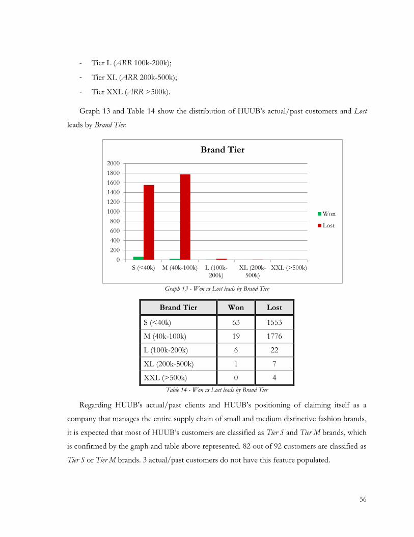
56

- Tier L (ARR 100k-200k);

- Tier XL (ARR 200k-500k);

- Tier XXL (ARR >500k).

Graph 13 and Table 14 show the distribution of HUUB’s actual/past customers and Lost

leads by Brand Tier.

Graph 13 - Won vs Lost leads by Brand Tier

Brand Tier Won Lost

S (<40k) 63 1553

M (40k-100k) 19 1776

L (100k-200k) 6 22

XL (200k-500k) 1 7

XXL (>500k) 0 4

Table 14 - Won vs Lost leads by Brand Tier

Regarding HUUB’s actual/past clients and HUUB’s positioning of claiming itself as a

company that manages the entire supply chain of small and medium distinctive fashion brands,

it is expected that most of HUUB’s customers are classified as Tier S and Tier M brands, which

is confirmed by the graph and table above represented. 82 out of 92 customers are classified as

Tier S or Tier M brands. 3 actual/past customers do not have this feature populated.

0

200

400

600

800

1000

1200

1400

1600

1800

2000

S (<40k) M (40k-100k) L (100k-200k)

XL (200k-500k)

XXL (>500k)

Brand Tier

Won

Lost

57

This fact is also represented in concern to Lost leads, only 33 leads are not classified as Tier

S or Tier M fashion brands. 338 leads do not have information about its Brand Tier.

4.2.4.15. Correlation between Number of Items, Price per Item,

Amount (ARR) and Brand Tier features

After analysing the last four features, some concerns that are relevant to clarify and to

discuss emerged. An interesting conclusion after the analysis of the mentioned features is the

inconsistency of data between them. As all these four features are correlated, that is Brand Tier

depends of the feature Amount (ARR) which depends on the feature Price per Item and Number of

Items, the number of missing values of the feature Brand Tier should not be less than none of

the previous features, as it happens. This fact along the pattern emerged among values of

Amount (ARR), motivated an explanation about this topic with HUUB’s sales representatives.

In regard to the common values of Amount (ARR), after exposing this concern to HUUB’s

marketing and sales team, it was said that at a certain moment in time, the value of Amount

(ARR) was automatically filled even when there was no accurate information about this

feature. Those common values were the average values of ARR of HUUB’s actual customers,

at that time.

The value 23484 corresponds to brands that only have Ecommerce as one of its sales

channels. The value 92592 relates to brands that have Wholesale, Wholesale and Ecommerce or

Own Stores as one of its sales channels. Lastly, the value 40000 was assigned when no

information about the brand’s sales channel was provided. It is important to state that this fact

is no longer a practice from HUUB. From a certain time on, ARR is only populated when the

necessary information is provided.

Moreover, after a meeting with HUUB’s sales representatives, it became clear that the most

accurate feature, among the ones that express a lead’s financial dimension, is Brand Tier. Precise

information about the Amount (ARR) feature takes time to gather, as it was already referred.

Throughout the sales cycle, at meetings or through conversations between HUUB’s sales

personnel and fashion brands’ representatives, information about lead’s activity and

commercial numbers is provided. Most of the times, a price per item is not even negotiated

58

and defined and the number of items per season is not accurately communicated, although

with approximate numbers it is possible to predict, with the due considerations, the expected

revenue of the potential customer. Thus, as this feature relates to a range of values, divided

into classes, sales representatives often opt to populate this feature firstly even when they do

not have exact information about a lead’s ARR. Thus, Brand Tier represents a good proxy of

the financial dimension of a potential customer.

4.3. Data Preparation

This step of the project consists of preparing the data to the Modelling stage and is a

relevant process of any data mining project. Feature selection, data transformation, data

cleaning and how to deal with the missing values, are major tasks of this step to assure that

data is accurate and suitable for the Modelling step.

4.3.1. Final feature selection

Feature selection can have a huge impact in the model’s performance. Table 15 presents

the features that were used to train and test the classification algorithms.

ID Deal Name

Independent Features

Deal Source

Brand Segment

Country

Main Market(s)

Sales Channel(s)

Ecommerce Platform

Production

Product’s Category

Brand Type

Followers

Table 15 - Feature Selection

One may wonder why the Deal Stage, Pipeline, Deal Owner, Number of Items, Price per Item,

Amount(ARR) and Brand Tier features were not included in the model. Regarding the features

59

Deal Stage, Pipeline and Deal Owner, these features were not included in the model, in order to

correctly train the machine learning algorithm to learn and predict the outcome of each lead

based on lead’s intrinsic characteristics and not on the pipeline/deal stage the lead is currently

in or who is the sales representative in charge of the sales process of certain lead, as it is not

the purpose of this project. Yet, when selecting future leads to contact, each lead will be on an

initial stage of any Pipeline; thus it did not make sense to select the feature Deal Stage to be

included in the training set.

Regarding the features Price per Item, Number of Items, Amount(ARR) and Brand Tier, although

these features provide information about the financial dimension of any fashion brand, which

is a crucial factor to HUUB, when prioritizing leads to engage firstly, these features are not

available and populated a priori, as it is very easily to understand. As it was already mentioned,

these are features that are only populated on an advanced stage of the sales process. Since the

objective of this approach is to apply the best performing machine learning model to new sales

leads and predict to each class they belong to, and then prioritize them given that outcome, it

was not suitable to include in the model features that those same new leads do not have

populated, in general. For this reason, these features were not included in the model.

On the other hand, the feature Followers was included in the model since it can be depicted

as a good proxy of the dimension of a brand, as if a brand has a high number of Instagram

Followers, the greater the chance of that fact is related to relevant revenue amount, and vice

versa.

4.3.2. Missing Values

Regarding the next steps of the project, it is also important to analyse the number of

observations with missing values and observations without missing values by class (Won and

Lost). Throughout the exploratory data analysis done in the previous section, it was possible to

conclude that this dataset deals with a lot of missing values. The following table shows a

balance of the number of missing values by feature and class.

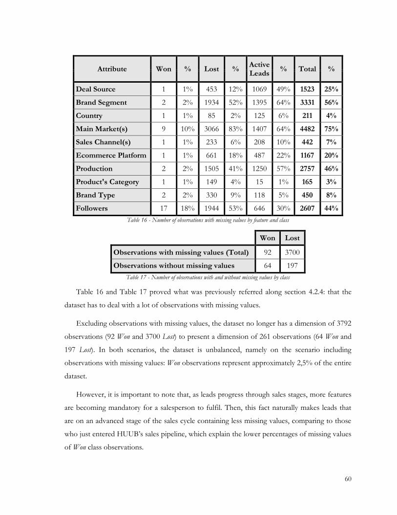
60

Attribute Won % Lost % Active Leads

% Total %

Deal Source 1 1% 453 12% 1069 49% 1523 25%

Brand Segment 2 2% 1934 52% 1395 64% 3331 56%

Country 1 1% 85 2% 125 6% 211 4%

Main Market(s) 9 10% 3066 83% 1407 64% 4482 75%

Sales Channel(s) 1 1% 233 6% 208 10% 442 7%

Ecommerce Platform 1 1% 661 18% 487 22% 1167 20%

Production 2 2% 1505 41% 1250 57% 2757 46%

Product's Category 1 1% 149 4% 15 1% 165 3%

Brand Type 2 2% 330 9% 118 5% 450 8%

Followers 17 18% 1944 53% 646 30% 2607 44%

Table 16 - Number of observations with missing values by feature and class

Won Lost

Observations with missing values (Total) 92 3700

Observations without missing values 64 197

Table 17 - Number of observations with and without missing values by class

Table 16 and Table 17 proved what was previously referred along section 4.2.4: that the

dataset has to deal with a lot of observations with missing values.

Excluding observations with missing values, the dataset no longer has a dimension of 3792

observations (92 Won and 3700 Lost) to present a dimension of 261 observations (64 Won and

197 Lost). In both scenarios, the dataset is unbalanced, namely on the scenario including

observations with missing values: Won observations represent approximately 2,5% of the entire

dataset.

However, it is important to note that, as leads progress through sales stages, more features

are becoming mandatory for a salesperson to fulfil. Then, this fact naturally makes leads that

are on an advanced stage of the sales cycle containing less missing values, comparing to those

who just entered HUUB’s sales pipeline, which explain the lower percentages of missing values

of Won class observations.

61

4.3.3. Data Transformation

As an outcome of the initial data understanding step, where the data preparation step

started, it was clear that there were some complexities regarding the dataset that would further

be object of data transformation, in order to be suitable for modelling.

Some data preparation was made before the data understanding step, as it was said before,

otherwise it would not be possible to do a proper data understanding step and conduct an

exploratory analysis of the dataset. Data was filled with no accuracy and too many different

values (that were the same value, only typed in a different way) appeared regarding some

features. As an example, considering Product Category feature, there were values such as Apparel;

Accessories and Accessories; Apparel which both refer to the same product category. Also some

typing errors emerged, so they had to be corrected so that the exploratory data analysis was

accurate. Yet, data in that form was not suitable for the model building step, thus, a correction

of these errors was done.

Categorical variables clearly dominate the dataset, as already mentioned. On top of that,

these categorical variables were populated in a not suitable way for modelling, as the below

image shows, with the features Main Market(s) and Sales Channel(s) as an example (Deal Name

was deleted for data privacy reasons).

Deal Name Main Market(s) Sales Channel(s)

Europe; Belgium; Germany; Switzerland Ecommerce; Wholesale

Asia; Middle East; USA & Canada Ecommerce; Wholesale

Asia; Central & South America Wholesale

Africa & ROW; Europe; USA & Canada Ecommerce; Wholesale

Asia; Middle East; USA & Canada Wholesale

Africa & ROW; Europe; USA & Canada Ecommerce; Wholesale

Asia; Europe; Italy Ecommerce; Own Stores

Table 18 - Data quality: Categorical Variables

It is expected that a fashion brand has more than one value regarding some features, as

previously described. An example is presented in Table 18, regarding the feature Main

62

Market(s). Indeed, data separated by “;” is not suitable for modelling and can compromise

model’s performance.

Due to that, in this stage of the process, feature transformation of the categorical variables

was performed. One approach to optimise the dataset emerged: one-hot encoding the

variables. One-hot encoding is a process in which categorical variables and its nominal values

are converted into an integer value so machine learning algorithms can perform better.

According to this approach, for each category, a new column is created, where the value is 1 if

for that observation the original feature assumes that value and 0 otherwise. Thus, it was

needed an additional layer of encoding schemes where dummy features were created for each

unique value or category out of all the distinct categories per feature. As an example, a brand

that its main market is China; Italy, would have the value 1 in the feature Main Market – Europe

and Main Market – Asia and the value 0 for the remaining features regarding Main Market(s)

feature.

Apart from the fact that this approach enabled the dataset to be suitable for modelling, it

also allowed the representation of categorical data to be more expressive.

The following features were then transformed: Main Market(s), Sales Channel(s), Production,

Product Category and Brand Type. As an example, regarding the feature Main Market(s), this

feature was transformed into the following: Main Market – Europe, Main Market – North

America, Main Market – Central & South America, Main Market – Asia, Main Market - Africa &

ROW, Main Market – Middle East and Main Market – Oceania.

A more comprehensive understanding of this approach can be consulted through the

example provided in Appendix B.

4.3.4. Label creation

Regarding the nature of this project, and motivated by the findings provided by the

literature review, this study addressed the problem on hand as a typical binary classification

machine learning problem.

As it was stated before, the distribution of fashion brands by class (Won vs Lost) is

provided by filtering the data by deal stages (see section 4.2.2).

63

Then, this approach consisted in developing a machine learning model that predicts the

class of each lead belongs to: Won or Lost, based on the historical dataset that contains leads

whose class and characteristics are known. The likelihood of any lead to turn into a customer is

the same as the confidence value that the machine learning algorithm assigns to all leads. It is a

value representing the probability that any lead has of becoming a customer, regarding its

characteristics.

The definition of the label (dependent variable) for this approach was straightforward. The

label was created by filtering the data by deal stages that tells which brands are actual/past

customers (Won) and which are Lost leads. A new variable called Is Client? was created from this

process which is the label (dependent variable) of this machine learning problem.

The label takes the value Won if a brand is already a client and the value Lost if the lead did

not result in a successful sale. Active leads, i.e. leads with open sales processes do not have the

label fulfilled.

4.4. Modelling

This step relates to discussing the selected machine learning algorithms applied to the

dataset regarding this project, taking into account what was already analyzed.

The purpose of this section is to apply suitable machine learning algorithms to predict if a

lead is classified as Won or Lost and use the confidence value assigned to each lead as the

likelihood of a lead to turn into customer.

Regarding this approach and the classification problem in hand, four supervised

classification algorithms were applied, motivated by the findings of the literature review on the

most widely used algorithms regarding similar studies: Decision Tree, Random Forest,

Gradient Boosted Tree and Logistic Regression.

To revisit, the dataset on hand is highly unbalanced (see section 4.3.2), as it was expected

regarding the concept of this data mining project. As referred on the literature review chapter

(see 2.7.3), sampling methods can be applied to handle class imbalance; thus, two types of

sampling methods were applied in this study to tackle this issue: undersampling and

oversampling methods.

64

In section 4.3.2 it is also possible to see the distribution of observations by classes (Won

and Lost) of the dataset. Furthermore, Table 17 illustrates the impact that the exclusion of

observations with missing values has on the size of the dataset.

Thus, apart from the two alternative sampling technique scenarios, this fact emerged the

creation of two more scenarios, taking this problem into account.

The reason behind this procedure was to include a scenario where the dataset was not

reduced drastically (which happened if observations with missing values were excluded), but

also to evaluate models’ performance on a dataset containing only observations without

missing values, the ideal situation. Given that, it is possible to evaluate how the models

perform on multiple scenarios.

Thus, four modelling scenarios were created, combining the two sampling methods with

the missing data/non-missing two dataset alternatives. Each one of the four selected machine

learning algorithms were applied to each one of the four scenarios created.

Scenarios were labeled as I, II, III and IV to provide an easier comprehension of this step

of the project.

Sampling techniques can be used to transform the training dataset in such a way that the

both classes have an equal distribution. Although, a crucial factor regarding these methods, is

to guarantee that these techniques are only applied on the training dataset, so that the model is

tested on a dataset that represent the actual state of the data. It is fundamental to ensure that

none observation is present on both datasets (training and testing) to obtain an unbiased

model’s performance evaluation. If this fact is not guaranteed, it can lead to overfitting.

With that being said, sampling methods were applied exclusively on the training dataset.

Undersampling, Oversampling and SMOTE techniques were selected. In the scenarios of

dataset with missing values, SMOTE cannot be applied; hence a simple random oversampling

of observations to equal the distribution of the classes was done.

Hold-out validation method was used to validate the performance of the models. Data was

partitioned into 70% for training and 30% for testing.

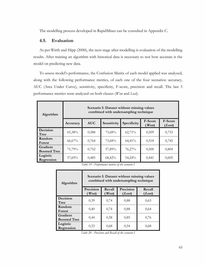
65

The modelling process developed in RapidMiner can be consulted in Appendix C.

4.5. Evaluation

As per Wirth and Hipp (2000), the next stage after modelling is evaluation of the modelling

results. After training an algorithm with historical data is necessary to test how accurate is the

model on predicting new data.

To assess model’s performance, the Confusion Matrix of each model applied was analyzed,

along with the following performance metrics, of each one of the four scenarios: accuracy,

AUC (Area Under Curve), sensitivity, specificity, F-score, precision and recall. The last 3

performance metrics were analyzed on both classes (Won and Lost).

Algorithm

Scenario I: Dataset without missing values combined with undersampling technique

Accuracy AUC Sensitivity Specificity F-Score (Won)

F-Score (Lost)

Decision Tree

65,38% 0,588 73,68% 62,71% 0,509 0,733

Random Forest

66,67% 0,764 73,68% 64,41% 0,518 0,745

Gradient Boosted Tree

71,79% 0,752 57,89% 76,27% 0,500 0,804

Logistic Regression

57,69% 0,485 68,42% 54,24% 0,441 0,605

Table 19 - Performance metrics of the scenario I

Algorithm

Scenario I: Dataset without missing values combined with undersampling technique

Precision (Won)

Recall (Won)

Precision (Lost)

Recall (Lost)

Decision Tree

0,39 0,74 0,88 0,63

Random Forest

0,40 0,74 0,88 0,64

Gradient Boosted Tree

0,44 0,58 0,85 0,76

Logistic Regression

0,33 0,68 0,54 0,68

Table 20 - Precision and Recall of the scenario I

66

Algorithm

Scenario II: Dataset without missing values combined with SMOTE technique

Accuracy AUC Sensitivity Specificity F-Score (Won)

F-Score (Lost)

Decision Tree

73,08% 0,750 78,95% 71,19% 0,588 0,800

Random Forest

71,79% 0,789 63,16% 74,58% 0,522 0,800

Gradient Boosted Tree

66,67% 0,710 52,63% 71,19% 0,435 0,764

Logistic Regression

67,95% 0,653 38,46% 72,88% 0,444 0,775

Table 21 - Performance metrics of the scenario II

Algorithm

Scenario II: Dataset without missing values combined with SMOTE technique

Precision (Won)

Recall (Won)

Precision (Lost)

Recall (Lost)

Decision Tree

0,47 0,79 0,91 0,71

Random Forest

0,44 0,63 0,86 0,75

Gradient Boosted Tree

0,37 0,53 0,82 0,71

Logistic Regression

0,53 0,38 0,83 0,73

Table 22 - Precision and Recall of the scenario II

Algorithm

Scenario III: Dataset with missing values combined with undersampling technique

Accuracy AUC Sensitivity Specificity F-Score (Won)

F-Score (Lost)

Decision Tree

94,11% 0,923 82,14% 94,41% 0,407 0,969

Random Forest

92,71% 0,964 92,86% 92,70% 0,385 0,961

Gradient Boosted Tree

81,28% 0,901 78,57% 81,35% 0,171 0,894

Logistic Regression

68,98% 0,769 78,57% 68,74% 0,111 0,812

Table 23 - Performance metrics of the scenario III

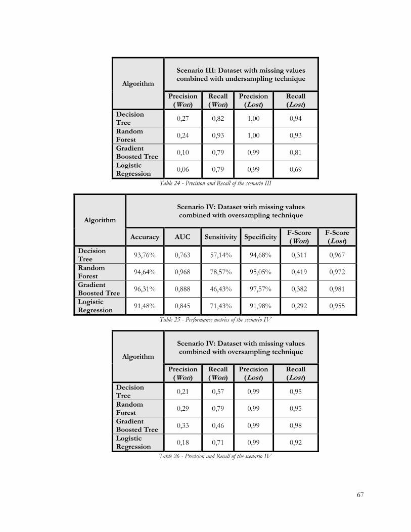
67

Algorithm

Scenario III: Dataset with missing values combined with undersampling technique

Precision (Won)

Recall (Won)

Precision (Lost)

Recall (Lost)

Decision Tree

0,27 0,82 1,00 0,94

Random Forest

0,24 0,93 1,00 0,93

Gradient Boosted Tree

0,10 0,79 0,99 0,81

Logistic Regression

0,06 0,79 0,99 0,69

Table 24 - Precision and Recall of the scenario III

Algorithm

Scenario IV: Dataset with missing values combined with oversampling technique

Accuracy AUC Sensitivity Specificity F-Score (Won)

F-Score (Lost)

Decision Tree

93,76% 0,763 57,14% 94,68% 0,311 0,967

Random Forest

94,64% 0,968 78,57% 95,05% 0,419 0,972

Gradient Boosted Tree

96,31% 0,888 46,43% 97,57% 0,382 0,981

Logistic Regression

91,48% 0,845 71,43% 91,98% 0,292 0,955

Table 25 - Performance metrics of the scenario IV

Algorithm

Scenario IV: Dataset with missing values combined with oversampling technique

Precision (Won)

Recall (Won)

Precision (Lost)

Recall (Lost)

Decision Tree

0,21 0,57 0,99 0,95

Random Forest

0,29 0,79 0,99 0,95

Gradient Boosted Tree

0,33 0,46 0,99 0,98

Logistic Regression

0,18 0,71 0,99 0,92

Table 26 - Precision and Recall of the scenario IV

68

5. Discussion

In this section, the performance of the four machine learning algorithms applied to each of

the four scenarios is discussed with the appropriate conclusions and suggestions.

When analyzing the performance of the models, one performance criteria was left out:

accuracy. Although it is one of the most widely used performance metrics to assess model’s

performance, in the presence of a data mining project with an unbalanced dataset, using this

metric could mislead any about the overall performance of the model. As an example, if a

dataset is composed by 500 observations (10 from class A and 490 from class B) and the

model predicts every observation to belong to class B, it still achieves a very high value of the

accuracy metric. Models could achieve high values of accuracy, simply by correctly predicting

the majority class, even if the minority class is totally wrongly predicted. However, that is not

the concept of a good overall model’s performance.

Since accuracy is not a reliable metric due to class imbalance of the dataset, other

performance metrics were considered.

AUC was the preferred criteria to obtain an overall estimate of the models’ performance.

This is a reliable metric when it comes to performance measurement of machine learning

classification problems as it tells how capable the model is of distinguish both classes (in this

case, between Won and Lost observations). AUC can assume values between 0 and 1. The

higher the value of AUC, the better is the model.

Along with the AUC metric, sensitivity and specificity metrics were also considered to

evaluate if the models categorized correctly the two classes. Sensitivity measures the percentage

of actual positive (Won) observations that were predicted correctly as positive and specificity is

used to determine the percentage of actual negative (Lost) observations that were predicted

correctly as negative. Also, the higher the value of sensitivity and specificity, the better is the

model.

Furthermore, one last metric was considered to measure the performance of the models:

F-score. This metric takes into account two other metrics: precision and recall.

69

Precision is simply the ratio of correct positive (negative) predictions out of all positive

(negative) predictions made by the model. It is a relevant metric in certain cases, where the cost

of a false positive (negative) is high.

Recall, also known as sensitivity, consists of the number of positive (negative) observations

the model correctly predicted as being positive (negative). Recall is an important metric in

projects where there is a high cost related to a false negative (positive).

Since in this study, both precision and recall measures are relevant, and since one metric

comes at the cost of another, F-score metric was also selected to evaluate models’

performance, as it considers both precision and recall metrics. Due to that fact, taking into

consideration the F-score metric, it is only needed to analyze one score rather than two

separate metrics (precision and recall). As for precision and recall, the F-score can be

calculated for each class of the dataset and it tells how precise and robust the classification

algorithm is. This metric can variate between 0 and 1. Thus, the higher the value of F-score,

the better is the model.

Moving now to the analysis of the models’ performance, when analyzing Table 19, Table

21, Table 23 and Table 25, taking the AUC metric in consideration, the first conclusion that

stands out is that models performed better on the scenarios of the original dataset i.e.,

including observations with missing values (scenario III and IV), namely on scenario III.

In addition, also considering the AUC metric, Random Forest algorithm outperforms the

remaining models on each one of the four scenarios. Indeed, the highest value of the AUC

metric, among the four scenarios, is achieved by the Random Forest algorithm on the scenario

IV (AUC of 0,968). On the other hand, Logistic Regression algorithm can be considered the

worst performing model, taking into account this performance metric (except on the scenario

IV where the Decision Tree algorithm performed worse).

However, given the context of this problem, the performance of the models cannot be

analyzed taking into account only the AUC metric, as it can be misleading. It is also relevant to

discuss how the models treated each class (Won and Lost), being that a false positive (Lost

observation predicted as Won) and a false negative (Won observation predicted as Lost) have

70

different but unwanted consequences in each case, for the company under study, given the

topic covered on this data mining project.

A false positive, that is, a Lost lead predicted as Won, would lead to waste of time and

resources, since sales representatives would be pursuing and investing time on a lead that was

misclassified as a lead with high likelihood of becoming a successful sale.

Moreover, a false negative can relate to a situation where a Won lead is predicted as Lost,

which could imply that efforts will not be allocated in the most efficient way and successful

sales opportunities will not be pursued.

Thus, sensitivity, specificity and F-score, combining precision and recall metrics, are given

higher relevance on this study as performance metrics to be maximized.

Overall, the highest values of sensitivity and specificity also occur on the scenario III,

meaning that most actual positive (Won) observations and also actual negative (Lost)

observations were predicted correctly as such by the models. Yet, Random Forest algorithm on

this scenario was the best model regarding sensitivity and specificity metrics, achieving 92,86%

and 92,70%, respectively, among the remaining scenarios and algorithms.

Until now, Random Forest algorithm on the scenario III seems to achieve a good overall

performance compared to the remaining scenarios and models, with an AUC of 0,964 (only

slightly outperformed by the Random Forest algorithm on the scenario IV, where achieved an

AUC of 0,968) and the highest values of sensitivity and specificity, as already referred.

In most problems, one could either give a higher priority to maximize precision, or recall,

depending upon the problem under study. As for the already mentioned reasons, in the

context of lead scoring, it is important to obtain high values of both metrics.

Hence, it is also important to analyze the F-score metric in order to dive deeper into the

performance of the models.

In general, on each one of the four scenarios, the values of the F-score for the majority

class (Lost) are higher than the values of the F-score for the Won class, for each one of the four

models applied. This fact is probably justified by the unbalanced dataset, where, in the two

71

scenarios with missing values (scenarios III and IV), 97,5% of the observations belong to the

Lost class (3700 out of 3792) and in the 2 scenarios where observations with missing values

were excluded (scenarios I and II), approximately 76% of the observations belong to the Lost

class (197 out of 261) (see section 4.3.2).

Despite the good overall performance of the AUC, sensitivity and specificity metrics of the

Random Forest within the scenario III, this model does not achieved quite good results

regarding F-score values for the Won class. The model achieved very good results regarding

precision and recall for the majority class (Lost), of approximately 1 and 0,93 respectively.

However the precision for the Won class was significantly lower (0,24), which is a major

setback of the quality of this model in this scenario.

The low value of the precision for the Won class, combined with the high value of

sensitivity, means that the Random Forest model predicted too many false positives, which

regarding the context of this problem and the topic of lead scoring, is not a good indicator of

the most suitable model. Also, every model of the scenario III do not present quite interesting

values of the F-score for the Won class (caused by the low values of precision for this class).

Thus, an analysis of the models of the remaining two scenarios (scenario I and II) is needed to

ascertain if any model achieved a better overall performance, taking into account all of the

performance metrics already referred.

Regarding AUC, on the scenarios excluding observations with missing values (scenario I

and II) the best model is also the Random Forest model, on the approach using the SMOTE

sampling technique (scenario II) achieving an AUC of 0,789. However, in regard to the

sensitivity metric, this model is outperformed by the Decision Tree model (63.16% compared

to 78.95%) on the same approach. Yet, the Random Forest model on this scenario treated

classes a bit differently. This model presented a value of 63,16% of sensitivity but 74,58%

regarding specificity, which means that is better at identifying observations from the majority

class (Lost) than from the minority class (Lost).

Furthermore, despite the fact that the Random Forest model on this approach achieved a

higher F-score for the Won class (0,522) than the Random Forest model on the scenario I

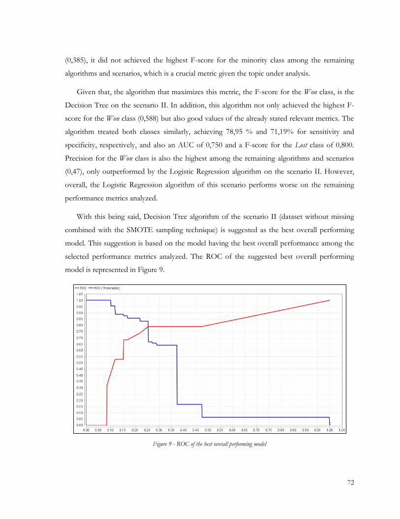
72

(0,385), it did not achieved the highest F-score for the minority class among the remaining

algorithms and scenarios, which is a crucial metric given the topic under analysis.

Given that, the algorithm that maximizes this metric, the F-score for the Won class, is the

Decision Tree on the scenario II. In addition, this algorithm not only achieved the highest F-

score for the Won class (0,588) but also good values of the already stated relevant metrics. The

algorithm treated both classes similarly, achieving 78,95 % and 71,19% for sensitivity and

specificity, respectively, and also an AUC of 0,750 and a F-score for the Lost class of 0,800.

Precision for the Won class is also the highest among the remaining algorithms and scenarios

(0,47), only outperformed by the Logistic Regression algorithm on the scenario II. However,

overall, the Logistic Regression algorithm of this scenario performs worse on the remaining

performance metrics analyzed.

With this being said, Decision Tree algorithm of the scenario II (dataset without missing

combined with the SMOTE sampling technique) is suggested as the best overall performing

model. This suggestion is based on the model having the best overall performance among the

selected performance metrics analyzed. The ROC of the suggested best overall performing

model is represented in Figure 9.

Figure 9 - ROC of the best overall performing model

73

Feature relevance of the suggested best overall performing model can be consulted in

Appendix D.

74

6. Manual approach – Scorecard

Motivated by the findings provided by the literature review and the insights gathered along

the exploratory data analysis pursued on section 4.2.4, a complementary approach to the

automated one is suggested. This approach consists of a non-automated solution: a scorecard

to be integrated along HUUB’s CRM platform (Hubspot).

As it was referred on the literature review section, CRM platforms provide useful tools to

the topic of lead scoring and lead prioritization. Furthermore, the so-called manual lead scoring

is widely used by many companies and organizations to rank their leads in order to prioritize

their sale efforts and resources towards leads with high perceived value to the organization.

The manual scoring system was elaborated sustained on the insights provided from the

exploratory data analysis done on section 4.2.4 and also based on the business know-how

gathered during the internship period. Furthermore, HUUB’s sales team promptly shared all its

expertise and vision on this topic and exchanged relevant information regarding the customer

acquisition process which was crucial to the design of the scorecard.

Features included on the scorecard were the same ones selected to the machine learning

assisted approach. Based on the insights extracted along the exploratory data analysis, given the

nature of some features and the ease to HUUB of converting leads that have certain

characteristics, greater relevance of those same features’ values was taken into account when

defining the scores to assign to new sales leads.

The most represented value of a certain feature would correspond to a higher score and

the less represented feature would correspond to a lower score, since higher represented

features would mean that HUUB has an advantage of targeting brands that have that

characteristic. The logic behind this is to assign higher points/values to what drives a

successful sale the most, after concluding what actual/past customers have in common.

The suggested scorecard to be integrated on HUUB’s CRM platform can be consulted in

Appendix E.

75

As new leads enter in HUUB’s sales pipeline, its overall score would be the sum of each

one of its features, according to the scorecard presented.

A lead could have the maximum score of 100.

The following paragraphs provide a more detailed explanation of the scoring criteria

designed.

Deal Source

It was possible to conclude through the exploratory analysis that most of HUUB’s

actual/past clients came through Organic and Referral sources. Although this fact should be

reflected on the score scale, most of the leads are contacted through an inside sales strategy or

prior to a tradeshow visit (Cold Contact and Fair, respectively) and this feature should not be of

a higher relevance when prioritizing which brand to contact firstly. The score scale designed

regarding the feature Deal Source reflects the ease to convert leads from Organic and Referral

sources, sustained by the previous analysis, establishing also a difference between leads from

intern profiling (Cold Contact and External Agency) and tradeshows’ leads (Fair), taking into

account business expertise from HUUB’s sales team.

Regarding leads generated from the External Agency, it is suggested not to assign any extra

points as a mean of prioritize leads from this source, given that any lead was converted from

this source yet, which might indicate that this source is delivering poor quality leads.

Brand Segment

After analyzing the insights extracted from the exploratory data analysis, accordingly to

what was concluded on section 4.2.4.2, the score scale defined reflect the high perceived value

to HUUB of fashion brands classified as Premium brands, since brands from this segment

represent 85% of HUUB’s actual/past clients. However, in spite of the major preponderance

of Premium brands on HUUB’s customer portfolio, HUUB does not intend to target this

segment only. As an organization that describes itself as a tech-startup that manages the entire

supply chain of distinctive fashion brands, HUUB also wants to include in its portfolio Value

and Luxury fashion brands. Thus, the score scale designed to this feature was based on these

major points.

76

Leads classified as Low Cost brands are not given any priority, as the points assigned to

these brands regarding this feature is suggested to be null. This conclusion is justified after the

exchange of information with HUUB’s sales team, that brands from this segment are not a

major target for the company, as the numbers corroborate (0 Won brands out of 6 total brands

contacted from this segment).

Country

The feature Country assumes a higher relevance when it comes to prioritize which brand

HUUB’s sales team should contact firstly. As it was concluded before, on section 4.2.4.3, most

of HUUB’s actual/past clients are Portuguese brands. Also, HUUB is trying to gain expression

and to position itself as the number one logistics player in the Portuguese fashion industry. It is

not only its long-term strategy, as the numbers already corroborate that, since 32 out of 92

customers are Portuguese fashion brands. Due to its relevance, a higher score scale was

defined to the feature Country. Higher values are suggested to assign to Portuguese, British,

French and Spanish brands, in particular, as they are the most represented countries on

HUUB’s customers portfolio.

Moreover, when sharing its expertise, HUUB’s sales team pointed out a relevant topic

related to the specificity of sales processes of Italian brands. The specificity and the reluctance

on cooperating along the process makes Italian brands a hard target to convert into a

customer, no matter how much effort is put into the process, according to HUUB’s expertise.

Numbers prove this fact, as any Italian fashion brand has ever become a HUUB’s customer,

despite the 354 Italian brands contacted already.

Due to that, it is suggested to assign a negative value to Italian brands, regarding this

feature. It is also suggested not to assign points to brands from Central & South America,

Africa, Asia and Oceania, as none of the brands from HUUB’s customer portfolio are from

any of these continents.

Main Market(s)

After analyzing HUUB’s customer portfolio on section 4.2.4.3, given the preponderance of

brands that have an European country or the European continent as their main market, it is

77

suggested that the score rules of this feature reflect the high perceived value that this type of

brands have for HUUB (77 out of 92 brands have at least an European country or the

European continent as one of its main market). As it was already referred, given the location of

HUUB’s warehouses (Portugal and Netherlands), the analysed numbers confirm that HUUB

finds it easier to convert leads that have the European continent or an European country as

Main Market, rather than brands that have its main market(s) on the Asian or American

continent, for example, due to the geographic location of HUUB’s warehouses and

consequently proximity to their main market(s).

The score rules of this feature do not include the assignment of points to brands that have

one (or many) of the following main markets: Central & South America, Middle East, Oceania

and Africa, supported by the insights provided on section 4.2.4.4.

Sales Channel

In section 4.2.4.5, it was possible to conclude that the major part of HUUB’s sales pipeline

leads have Ecommerce and/or Wholesale as its main sales channel. This feature is not quite

relevant to define which lead to contact first and it is not crucial to define the likelihood of a

lead to turn into a customer. However, the score rule of this feature reflects the difference

between brands that sell through Ecommerce/Wholesale and brands that sells through Own Stores

or Marketplace, as it is not suggested to assign points to brands that sell through Own Stores or

Marketplace, as they represent a minority of HUUB’s customer portfolio.

Ecommerce Platform

As it was stated before in section 4.2.4.6, this feature is crucial to ascertain the likelihood of

a lead becoming a customer. There are many Ecommerce platforms in the market, but HUUB

does not integrate with all of them, logically. Hence, if a brand operates through a platform

that integrated with HUUB’s platform the chance of converting that specific brand into a

client is greatly increased, which explains the importance of this feature.

Given that, higher score scale was defined to this feature and higher scores are suggested

to be assigned to leads that operate through one of the following platforms: Shopify, Prestashop

78

and WooCommerce, since most of HUUB’s actual/past customers operate through one of this

Ecommerce platforms.

Production

This feature also has a high impact when defining the likelihood of a brand to turn into a

customer. Since HUUB is a Portuguese start-up with a warehouse located in Maia, Portugal,

the fact that 74 out of 92 actual/past clients have its production in Portugal is not surprising.

Brands that have its production centre located in Portugal seems to be an advantage to HUUB

and then a relevant topic when it comes to define the likelihood of a lead to turn into a

customer and which brand to contact firstly.

Hence, a higher score scale was assigned to this feature and higher values are suggested to

assign to brands that have its production in Portugal. The scores were assigned after analysing

the statistical distribution of this feature of HUUB’s actual/past clients on section 4.2.4.7.

Product Category

It was possible to conclude through the exploratory analysis discussed on section 4.2.4.8,

that most of HUUB’s actual/past clients sell Apparel products. Although this fact should be

reflected on the score scale, this feature should not be relevant when prioritizing which brand

to contact firstly and to define the likelihood of a lead to turn into a customer, as it is not

important to HUUB to distinct between Apparel brands and brands that commercialize other

product categories, as it is reflected on Appendix E.

Brand Type

HUUB has developed throughout the years a good position on Kids fashion market, as 35

out of 92 HUUB’s clients are Kids fashion brands. Yet, it is not HUUB’s strategy to focus only

on this type of brands. Thus, although this fact should be reflected on the score scale of this

feature, this feature should not be too relevant when prioritizing which brand to contact firstly,

as it is not relevant to distinct between a Kids fashion brand or an Adult fashion brand.

However, it is suggested to assign lower scores to other types of brands than Kids fashion

brands.

79

Followers

The last feature to be explained is Followers.

Since Brand Tier information is not possible to obtain on an a priori moment of contacting a

lead for the first time, a feature like Followers could have a relevant impact on determining the

perceived value that a certain lead might have to HUUB.

As it was described before, Brand Tier feature represents brand’s dimension, accordingly to

a scale defined by HUUB’s sales team. Since HUUB’s sales representatives do not have this

kind of information when selecting which lead to contact in the first place, the feature Followers

could be a good proxy that indicates the potential financial dimension of a brand, as the higher

the number of followers on Instagram, the bigger a brand might be. HUUB is described as a

“Brand Accelerator”, in charge of managing the logistics of small and medium distinctive

fashion brands. However, as is common to many businesses, as the business grows, the focus

and strategy might change. Thus, it is normal for HUUB to shift is strategy to conquer bigger

fashion brands to its client portfolio.

The score scale defined to this feature reflects this conclusion. Despite the fact that most

of HUUB’s clients are Tier S and Tier M fashion brands (82 out of 92), it is suggested to assign

higher scores to brands that have the highest number of followers on Instagram, suggesting a

higher perceived value to HUUB.

6.1. Automated lead scoring system vs Manual lead scoring scorecard

One of the critics that some authors point out on their studies regarding this topic under

analysis, is that manual lead scoring scorecards designed by many companies and embedded in

CRM platforms, are, most of the times, based on gut feeling and/or intuition and not properly

supported by data and facts.

However, along this project, an appropriate analysis of HUUB’s customer database

combined with business knowledge and market expertise were the foundation for the

scorecard purposed.

80

Furthermore, HUUB’s current situation regarding the selection of which leads to contact

firstly is mostly ad-hoc.

Thus, a manual lead scoring scorecard like the one addressed in this section brings value

on its own and represents an improvement to HUUB’s current situation. It is firmly believed

that it is a baseline solution and an improvement to HUUB current situation regarding the

topic of customer acquisition process, namely to the first step of selecting which leads to

target in the first place, since HUUB does not have any kind of lead scoring system at the

moment.

Even though the advantages of a manual lead scoring system seem quite obvious, it also

has disadvantages.

A manual lead scoring system can increase sales teams’ productivity, as referred by

academics. However, it can be a time-consuming task, which is one of the major setbacks of a

manual approach. It involves analyzing historical data, exchange information with the ones on

the field (sales teams), combine both information and create a lead scoring system, which is

not a short time process.

Yet, a scorecard like the one developed along this project is not something that is created

and prevails along the years. As new feedback is provided by sales teams, new leads are

converted into customers and others do not, and new data about the customer acquisition

process is gathered. Thus, the manual lead scoring system designed might need to be tuned to

guarantee that it remains accurate with what is happening in reality and with that new

information provided. Furthermore, if the company under analysis (or any other company)

shifts its strategy to a new market or to another type of leads, its optimal target changes too.

Hence, the scorecard previously designed and used by the company might be outdated which

also might imply the design of a whole new manual lead scoring scorecard and, consequently,

another longtime process.

All of these previously mentioned points require even more time to be spent by marketing

and sales department, thus a more robust solution was provided, with the application of

machine learning algorithm to predict the outcome of a sales lead.

81

By developing a machine learning assisted lead scoring system, all the major disadvantages

of a manual lead scoring system explained on the previous paragraphs are overcome. In fact,

the solution provided takes the traditional approach addressed on the previous section to the

next level.

With an automated solution like the one suggested, the lead scoring system can be updated

in real time, which overcome the main limitation of a manual approach as a time-consuming

process. Also, as new leads result in successful sales along time, an automated lead scoring

system as the sufficient capability to learn the new characteristics of those newest converted

leads and, given that new information, predict the outcome of new leads that enter on the sales

pipeline. It also frees up some time since with an automated lead scoring system sales teams no

longer have to track leads manually.

Furthermore, it revolutionizes the traditional lead scoring system that requires a lot human

intervention, hence, a more costly process in comparison with a more automated one, that do

not require such time and human intervention.

To conclude, the lead scoring scorecard designed must be depicted as a baseline

foundation for the lead scoring process of the company under analysis. However, since the

organization under analysis has the resources and infrastructures to gather data about

customers and leads, should aim to implement a more reliable tool like the automated lead

scoring system suggested, to get the maximum benefit from the data collected. Moreover, this

solution can overcome the previously mentioned limitations of a manual scoring solution, as

no bias, gut feeling or intuition are allowed.

82

7. Final Remarks

7.1. Conclusions

This project aimed to develop a solution regarding the problem of lead scoring as a critical

step of the customer acquisition process. Although this work is directed to a specific

organization, it is a topic and a concern to many companies, regardless of the industry where it

operates or its dimension.

Given the problem in hand, two approaches were suggested: a manual lead scoring system,

with the development of a lead scorecard as a complement to an automated approach, with the

usage of predictive analytics and machine learning to develop a classification algorithm that can

predict the likelihood of a lead to become a customer, i.e. if it will be classified as Won or Lost.

Supported by the findings collected through the research of studies published by the

scientific community, different supervised classification algorithms were applied: Decision

Tree, Random Forest, Gradient Boosted Trees and Logistic Regression. Different scenarios

were created and analyzed concerning the amount of observations with missing values on the

dataset and the unequal distribution of observations between both classes: Won and Lost. To

address the latter, different sampling techniques (undersampling, oversampling and SMOTE)

were applied to overcome the class imbalance problem.

Among the 4 scenarios, Decision Tree algorithm within scenario II was the best overall

performance model. This model is suggested as the best performing model as it achieved the

best overall performance among the relevant performance metrics analyzed, suitable to this

problem under study. Although, if the project had a different objective as the one in study, the

overall value of each model could change, and the selected model could be a different one.

To sum up, this study intended not only to suggest a binary approach solution designed to

a Portuguese startup in regard to the problematic of lead scoring, but also to contribute to

close the gap founded on the academic community related to predictive lead scoring. With this

project, we aimed to gather relevant papers and studies that could support and serve as a

foundation to the topic under analysis. Furthermore, after providing appropriate theoretical

and contextual information, the present study also used an open access tool, available to the

83

entire academic community but also to companies, as it is RapidMiner. A current gap on the

academic published relates to this fact, as most of the studies about the topic under analysis

use custom algorithms or advanced tools used by data scientists. Thus, this study aims to

provide basic, but useful concepts regarding data mining and predictive analytics topics and

also demonstrate the usage of RapidMiner, a well-known and user-friendly data mining

platform. With that being said, it is expected that this report provides valuable knowledge and

encourages marketers, sales personnel, small companies without solid information technology

structures and no knowledge of data mining techniques, to be part of the growing trend that

the entire world is facing.

7.2. Limitations and Further Suggestions

In concern to further suggestions, some areas of future and interesting work have been

brought to light along the progress of this study. An interesting topic of future research would

be to prioritize leads not only regarding its likelihood of resulting in a successful sale but also

to its expected revenue. Thus, a taskforce to study or to develop a model to predict a lead

Brand Tier, based on Instagram followers, for example, would be a valuable improvement to

HUUB’s status quo. In fact, one lead could have a higher likelihood of becoming a customer;

however, one might have higher expected revenue. This fact should be more relevant to

HUUB’s sales managers instead of a simple purchase probability since they could allocate

resources and efforts in a different way if such information was provided.

It is also suggested to incorporate on the CRM platform features that illustrate and relate

to the dynamic part of a sales pipeline, that is, behavioral features. Even though HUUB’s leads

are gathered from offline sources, and thus it is not possible to gather lead’s online activity,

other behavioral features might be created, regarding interactions between HUUB’s sales

representative and the lead itself. Although Duncan and Elkan (2015) concluded that high

quality leads can be identified even when only demographic features are available, the study

provided by Yan, Zhang, et al. (2015) suggest that activity features carry valuable information

about the interest of the lead and what could trigger a successful sale. However, the approach

suggested by these authors relies too much on the presence/absence of certain features, which

in many cases are not populated by sales team. A good example is the company analyzed on

84

this study, where too many missing values emerged, even on demographic features, as already

referred.

This fact leads to the main constraint of this study that it is relevant to point out.

HUUB’s data quality is quite poor, with too many missing values and non-coherent data,

which consisted of a limitation to this project. HUUB should improve on this topic in order to

enable better data mining projects and hence better business decisions too.

Regarding the significant amount of missing values, this fact meant that the training dataset

was reduced considerably given its potential dimension on 2 of the 4 scenarios created. A more

robust training dataset could lead to a better model’s performance and useful insights, as too

many Lost leads were excluded due to a significant number of missing values among its

features. It is comprehensible that some features are only populated on an advanced stage of

the sales process. However too many leads with closed sales cycles (Won and Lost) had missing

values on features that should be quite mandatory to be populated on certain stages of the

sales process.

Besides the enormous amount of missing values among almost every HUUB’s sales

pipeline features, data populated on the CRM platform was also not typed on the most

appropriate and suitable way to work on, either to develop data mining projects or just to

extract simple insights. Yet, too many typing errors emerged which made the data preparation

step the most exhaustive part of the project.

Thus, a more standardized way of populating features on HUUB’s CRM platform is

suggested and it is firmly believed that it will help in further data mining projects, either simple

or more complex ones. A suggestion on this topic is to create closed features and non-open

field ones, so that typing errors do not arise. Yet on this topic, to follow an approach similar to

the one adopted on this study regarding one-hot encoding variables is highly suggested. With

this approach, values will not be separated by “;”, as demonstrated on Table 18, which, once

again, will make any type of data analysis a lot more accurate and with less time expended,

hence, less money spent.

85

References

Abbott, D. (2014). Applied predictive analytics: Principles and techniques for the

professional data analyst: John Wiley & Sons.

Ang, L., & Buttle, F. (2006). Managing for successful customer acquisition: An exploration.

Journal of Marketing Management, 22(3-4), 295-317.

Benhaddou, Y., & Leray, P. (2017). Customer Relationship Management and Small Data—

Application of Bayesian Network Elicitation Techniques for Building a Lead Scoring Model.

Paper presented at the 2017 IEEE/ACS 14th International Conference on Computer Systems

and Applications (AICCSA).

Breiman, L. (2001). Random forests. Machine Learning, 45(1), 5-32.

Brynjolfsson, E., & McElheran, K. (2016). The rapid adoption of data-driven decision-

making. American Economic Review, 106(5), 133-139.

Chawla, N. V., Bowyer, K. W., Hall, L. O., & Kegelmeyer, W. P. (2002). SMOTE:

synthetic minority over-sampling technique. Journal of artificial intelligence research, 16, 321-

357.

Chou, P. B., Grossman, E., Gunopulos, D., & Kamesam, P. (2000). Identifying

prospective customers. Paper presented at the Proceedings of the sixth ACM SIGKDD

international conference on Knowledge discovery and data mining.

D’Haen, J., & Van den Poel, D. (2013). Model-supported business-to-business prospect

prediction based on an iterative customer acquisition framework. Industrial Marketing

Management, 42(4), 544-551. doi:10.1016/j.indmarman.2013.03.006

Duncan, B. A., & Elkan, C. P. (2015). Probabilistic Modeling of a Sales Funnel to Prioritize

Leads. Paper presented at the Proceedings of the 21th ACM SIGKDD International

Conference on Knowledge Discovery and Data Mining - KDD '15.

Farquad, M. A. H., Ravi, V., & Raju, S. B. (2014). Churn prediction using comprehensible

support vector machine: An analytical CRM application. Applied Soft Computing, 19, 31-40.

86

Friedman, J. H. (2002). Stochastic gradient boosting. Computational statistics data analysis,

38(4), 367-378.

Gulia, P. (2016). Comprehensive Study of Open-Source Big Data Mining Tools.

International Journal of Artificial Intelligence and Knowledge Discovery, 6(1).

Hubspot. (2020). CRM software. https://www.hubspot.com/. (Last access on:

06/09/2020)

Järvinen, J., & Taiminen, H. (2016). Harnessing marketing automation for B2B content

marketing. Industrial Marketing Management, 54, 164-175.

Kawas, B., Squillante, M. S., Subramanian, D., & Varshney, K. R. (2013). Prescriptive

analytics for allocating sales teams to opportunities. Paper presented at the 2013 IEEE 13th

International Conference on Data Mining Workshops.

Kincaid, J. W. (2003). Customer relationship management: getting it right! : Prentice Hall

Professional.

Kuhn, M., & Johnson, K. (2013). Applied predictive modeling (Vol. 26): Springer.

Monat, J. (2011). Industrial sales lead conversion modeling. Marketing Intelligence

Planning, 29, 178-194.

Mortensen, S., Christison, M., Li, B., Zhu, A., & Venkatesan, R. (2019). Predicting and

Defining B2B Sales Success with Machine Learning. Paper presented at the 2019 Systems and

Information Engineering Design Symposium (SIEDS).

Ngai, E. W. T. (2005). Customer relationship management research: An academic literature

review and classification (1992-2002). Marketing Intelligence & Planning, 23, 582-605.

Ngai, E. W. T., Xiu, L., & Chau, D. C. K. (2009). Application of data mining techniques in

customer relationship management: A literature review and classification. Expert Systems with

Applications, 36(2), 2592-2602. doi:10.1016/j.eswa.2008.02.021

87

Nygård, R., & Mezei, J. (2020). Automating Lead Scoring with Machine Learning: An

Experimental Study. Paper presented at the 2020 53rd Hawaii International Conference on

System Sciences.

Parvatiyar, A., & Sheth, J. (2001). Customer relationship management: Emerging practice,

process, and discipline. Journal of Economic Social Research, 3(2).

Paschen, J., Wilson, M., & Ferreira, J. (2020). Collaborative intelligence: How human and

artificial intelligence create value along the B2B sales funnel. Business Horizons, 63(3), 403-

414.

Patterson, L. (2007). Marketing and sales alignment for improved effectiveness. Journal of

Digital Asset Management, 3(4), 185-189.

Peng, C.-Y. J., Lee, K. L., & Ingersoll, G. M. (2002). An introduction to logistic regression

analysis and reporting. The journal of educational research, 96(1), 3-14.

Prati, R. C., Batista, G. E., & Monard, M. C. (2009). Data mining with imbalanced class

distributions: concepts and methods. Paper presented at the 2009 Indian International

Conference Artificial Intelligence.

Quinlan, J. R. (1986). Induction of decision trees. Machine Learning, 1(1), 81-106.

Shaw, M. J., Subramaniam, C., Tan, G. W., & Welge, M. E. (2001). Knowledge

management and data mining for marketing. Decision support systems, 31(1), 127-137.

Söhnchen, F., & Albers, S. (2010). Pipeline management for the acquisition of industrial

projects. Industrial Marketing Management, 39(8), 1356-1364.

Sokolova, M., Japkowicz, N., & Szpakowicz, S. (2006). Beyond accuracy, F-score and

ROC: a family of discriminant measures for performance evaluation. Paper presented at the

2006 Australasian joint conference on artificial intelligence.

Swift, R. S. (2001). Accelerating customer relationships: Using CRM and relationship

technologies: Prentice Hall Professional.

88

Syam, N., & Sharma, A. (2018). Waiting for a sales renaissance in the fourth industrial

revolution: Machine learning and artificial intelligence in sales research and practice. Industrial

Marketing Management, 69, 135-146.

Wirth, R., & Hipp, J. (2000). CRISP-DM: Towards a standard process model for data

mining. Paper presented at the Proceedings of the 4th international conference on the practical

applications of knowledge discovery and data mining.

Yan, J., Gong, M., Sun, C., Huang, J., & Chu, S. M. (2015). Sales pipeline win propensity

prediction: a regression approach. Paper presented at the 2015 IFIP/IEEE International

Symposium on Integrated Network Management (IM).

Yan, J., Zhang, C., Zha, H., Gong, M., Sun, C., Huang, J., . . . Yang, X. (2015). On machine

learning towards predictive sales pipeline analytics. Paper presented at the Twenty-ninth AAAI

conference on artificial intelligence.

89

Appendix A: Features Description

Feature Description Type

Deal Name Name of the fashion brand (lead). Categorical

Deal Owner Sales representative who is in charge of the sales process

of the lead. Categorical

Pipeline Pipeline where the lead is at the moment. Categorical

Deal Stage Stage of the lead in its current pipeline. Categorical

Deal Source

Information about the origin of the lead, how the lead entered on HUUB’s Sales Pipeline. Its source can be one of the following: Fair, Cold Contact, Organic, Referral (through an HUUB’s actual client) or External Agency.

Categorical

Brand Segment

Information about the segment of the fashion brand (lead). It can be a Low Cost brand, Luxury brand, Premium brand

or a Value brand. Categorical

Country Country of origin of the brand. Categorical

Main Market(s)

Market(s) to where the brand sells the most. Categorical

Sales Channel(s)

Channel(s) through which the brand sells its products. The sales channels are the following: Ecommerce, Wholesale,

Own Stores and Marketplace. Categorical

Ecommerce Platform

Information of what platform the brand uses to manage its online business.

Categorical

Production’s Country

Information about in which country (or countries) the brand produces its products.

Categorical

Product’s Category

Any fashion brand can sell products from one or many of the following categories: Accessories, Apparel, Footwear,

Home, Swimwear, Underwear and Other. Categorical

90

Brand Type This variable can assume one of the following values:

Adult (if the brand sells products to both Men and Women), Men, Women, Home, Kids, and Other.

Categorical

Followers Number of followers on Instagram social network. Numerical

Number of Items

Number of items (shoes, t-shirts, shirts, etc) that a brand expects to sell per season.

Numerical

Price per Item

HUUB charges a price for every item that a brand stocks on HUUB’s warehouse. This variable gives information

about this topic. Numerical

Amount (ARR)

It gives information about how much revenue HUUB expect to generate in a year, regarding a specific customers and its expected annual sales. It is related with the price per

item and the number of items per season.

Numerical

Brand Tier

HUUB established a scale to classify its leads taking into account its ARR. The scale is the following: S(<40k), M(40k-100k), L(100k-200k), XL(200k-500k) and XXL

(>500k).

Categorical

Table 27 - Features description

91

Appendix B: One-Hot Encoding

Main Market(s)

Main Market Europe

Main Market North

America

Main Market

Central & South

America

Main Market

Asia

Main Market

Africa & ROW

Main Market Middle

East

Main Market Oceania

Asia; Middle East; USA & Canada

0 1 0 1 0 1 0

Asia; Central & South America

0 0 1 1 0 0 0

Europe 1 0 0 0 0 0 0

Africa & ROW; Europe

1 0 0 0 1 0 0

China; Italy 1 0 0 1 0 0 0

Europe; Portugal; Spain

1 0 0 0 0 0 0

Switzerland; Sweden

1 0 0 0 0 0 0

Table 28 – Examples of feature transformation of the feature Main Market(s)

Sales Channel(s) Sales

Channel Ecommerce

Sales Channel

Wholesale

Sales Channel

Marketplace

Sales Channel

Own Stores

Ecommerce; Own Stores; Wholesale 1 1 0 1

Ecommerce; Wholesale 1 1 0 0

Ecommerce; Marketplace; Wholesale 1 1 1 0

Ecommerce 1 0 0 0

Table 29 – Examples of feature transformation of the feature Sales Channel(s)

Production Production

Portugal Production

Europe

Production North

America

Production Central & South America

Production Asia

Production Africa

Production Oceania

France; Portugal

1 1 0 0 0 0 0

China; Portugal

1 0 0 0 1 0 0

Brazil; USA 0 0 1 1 0 0 0

Asia; Germany

0 1 0 0 1 0 0

Europe; Tunisia

0 1 0 0 0 1 0

Table 30 - Examples of feature transformation of the feature Production

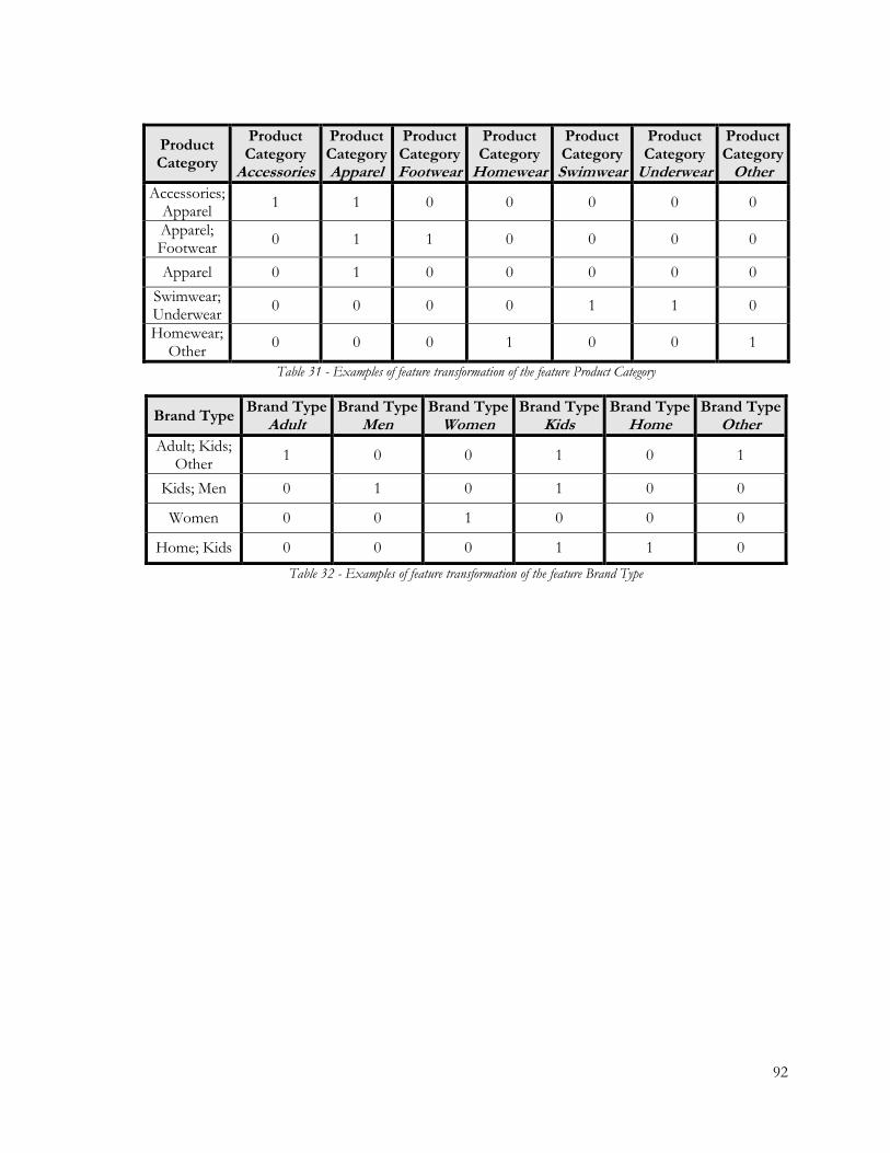
92

Product Category

Product Category

Accessories

Product Category Apparel

Product Category Footwear

Product Category

Homewear

Product Category

Swimwear

Product Category

Underwear

Product Category

Other

Accessories; Apparel

1 1 0 0 0 0 0

Apparel; Footwear

0 1 1 0 0 0 0

Apparel 0 1 0 0 0 0 0

Swimwear; Underwear

0 0 0 0 1 1 0

Homewear; Other

0 0 0 1 0 0 1

Table 31 - Examples of feature transformation of the feature Product Category

Brand Type Brand Type

Adult Brand Type

Men Brand Type

Women Brand Type

Kids Brand Type

Home Brand Type

Other

Adult; Kids; Other

1 0 0 1 0 1

Kids; Men 0 1 0 1 0 0

Women 0 0 1 0 0 0

Home; Kids 0 0 0 1 1 0

Table 32 - Examples of feature transformation of the feature Brand Type

93

Appendix C: RapidMiner Modelling Process

Figure 10 - RapidMiner modelling process within the scenario I (dataset without missing values combined with the undersampling technique)

94

Figure 11 - RapidMiner modelling process within the scenario II (dataset without missing values combined with the SMOTE technique)

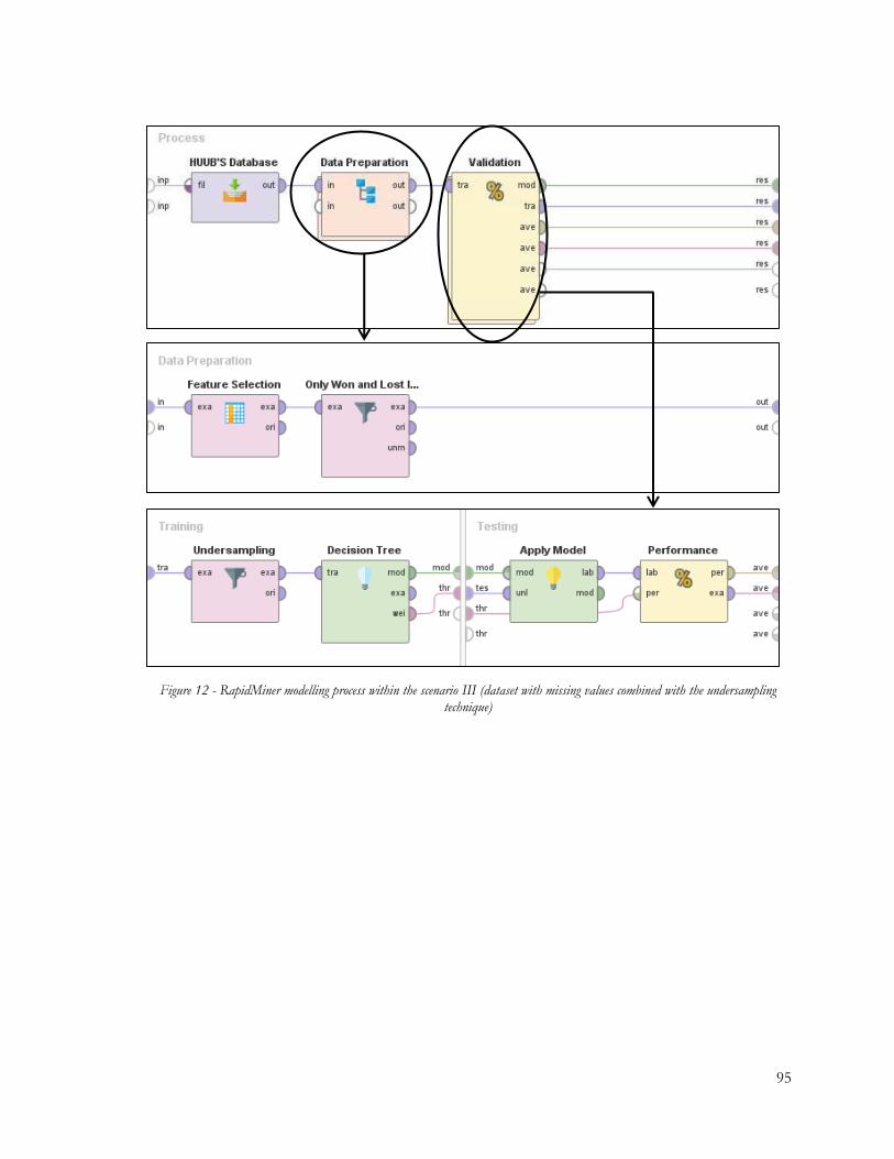
95

Figure 12 - RapidMiner modelling process within the scenario III (dataset with missing values combined with the undersampling technique)

96

Figure 13 - RapidMiner modelling process within the scenario IV (dataset with missing values combined with the oversampling technique)

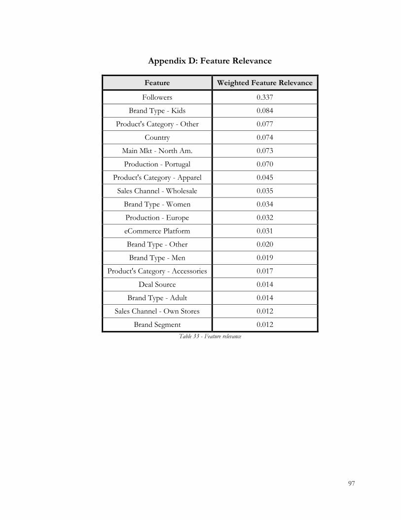
97

Appendix D: Feature Relevance

Feature Weighted Feature Relevance

Followers 0.337

Brand Type - Kids 0.084

Product's Category - Other 0.077

Country 0.074

Main Mkt - North Am. 0.073

Production - Portugal 0.070

Product's Category - Apparel 0.045

Sales Channel - Wholesale 0.035

Brand Type - Women 0.034

Production - Europe 0.032

eCommerce Platform 0.031

Brand Type - Other 0.020

Brand Type - Men 0.019

Product's Category - Accessories 0.017

Deal Source 0.014

Brand Type - Adult 0.014

Sales Channel - Own Stores 0.012

Brand Segment 0.012

Table 33 - Feature relevance

98

Appendix E: HUUB’s Lead Scoring Scorecard

DEAL SOURCE POINTS

Organic +5

Referral +5

Fair +3

Cold Contact +2

External Agency -

BRAND SEGMENT POINTS

Premium +5

Value +3

Luxury +3

Low Cost -

COUNTRY POINTS

Portugal +20

United Kingdom +10

France +10

Spain +10

Germany +7

Denmark +7

Other European Countries +5

USA +3

Italy -10

Canada -

Central & South America Countries -

Asia Countries -

Oceania Countries -

Africa Countries -

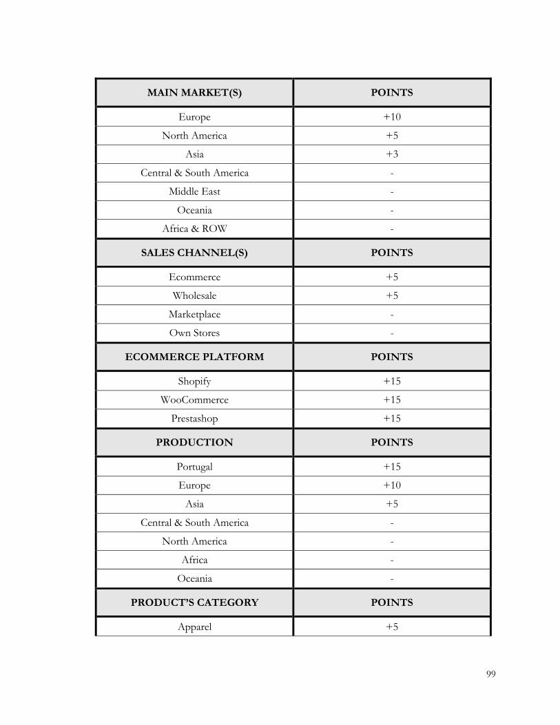
99

MAIN MARKET(S) POINTS

Europe +10

North America +5

Asia +3

Central & South America -

Middle East -

Oceania -

Africa & ROW -

SALES CHANNEL(S) POINTS

Ecommerce +5

Wholesale +5

Marketplace -

Own Stores -

ECOMMERCE PLATFORM POINTS

Shopify +15

WooCommerce +15

Prestashop +15

PRODUCTION POINTS

Portugal +15

Europe +10

Asia +5

Central & South America -

North America -

Africa -

Oceania -

PRODUCT’S CATEGORY POINTS

Apparel +5

100

Footwear +2

Accessories +1

Homewear -

Swimwear -

Underwear -

Other -

BRAND TYPE POINTS

Kids +5

Adult +4

Men +4

Women +3

Home -

Other -

FOLLOWERS POINTS

<1k -

1k-5k -

5k-10k +5

10k-25k +6

25k-50k +7

50k-100k +8

100k-200k +10

>200k +15

Table 34 - HUUB's Lead Scoring Scorecard