A Power system Protection scheme combining Impedance ...
199
A Power system Protection scheme combining Impedance Measurement and tavelling 'W'aves: Software and frardware Implementation by Vajira Pathirana A dissertation submitted to the Faculty of Graduate Studies in partial fulfillment of the requirements for the degree of Doctor of Philosophy The Department of Electrical and Computer Engineering The University of Manitoba Winnipeg, Manitoba, Canada @ April 2004
-
Upload
khangminh22 -
Category
Documents
-
view
4 -
download
0
Transcript of A Power system Protection scheme combining Impedance ...

A Power system Protection scheme combining ImpedanceMeasurement and tavelling 'W'aves: Software and frardware
Implementation
by
Vajira Pathirana
A dissertation submitted to the Faculty of Graduate Studies in partial fulfillment of
the requirements for the degree of
Doctor of Philosophy
The Department of Electrical and Computer Engineering
The University of Manitoba
Winnipeg, Manitoba, Canada
@ April 2004
TIIE UNTVERSITY OF MANITOBA
F'ACULTY OF GRADUATE STUDIES,rtr¡ttr*
COPYRIGHT PERMISSION
A Power System Protection Scheme Combining Impedance Measurement and TravellingWaves: Software and Hardware Implementation
BY
Vajira Pathirana
A ThesislPracticum submitted to the Facutty of Graduate Studies of The University of
Manitoba in partial fulfillment of the requirement of the degree
of
DOCTOR OF PHILOSOPHY
Vajira Pathirana @2004
Permission has been granted to the Library of the University of Manitoba to lend or sell copies ofthis thesis/practicum, to the National Library of Canada to microfilm this thesis and to lend or sellcopies of the film, and to University Microfilms Inc. to pubtish an abstract of this thesis/practicum.
This reproduction or copy of this thesis has been made availabte by authority of the copyrightowner solely for the purpose of private study and research, and may only be reproduced and
copied as permitted by copyright laws or with express written authorization from the copyrightovyner.

To my loving parents

Acknowledgements
I would like to express my sincere thanks to Prof.P.G. Mclaren for his continuous advice,
guidance and encouragement throughout the course of this work. I consider myself priviteged
to have had the opportunity to work under his guidance. I greatly appreciate the advice and
assistance received from Dr.Udaya Annakkage to complete my research. I am also grateful
to Mr.Adrian Castro of Maniioba Hydro for his advice and guidance. I must also thank
the technical staff at the Department of Electrical and Computer Engineering, especially
Mr.Erwin Dirks and Mr.Alan McKay for their valuable support.
I wish to thank Dr.Rohitha Jayasinghe and Dr.Dharshana Muthumuni of Manitoba
HVDC Research Center, Mr.Tom Hendrick of Texas Instruments fnc., Mr.Steve Zachman
and Mr.Bill Pitman of Hyperception Inc., and Mr.Hugh Pollitt-Smith of Canadian Micro-
electronics Corporation for their technical assistance. The financial support received from
Manitoba Hydro, the Faculty of Graduate Studies at the University of Manitoba and the
National Science and Engineering Research Council is greatly appreciated. I must also ex-
press my gratitude to the staff of the Center for Advanced Power Systems and National
High Magnetic Fields Laboratory at the Florida State Universit¡ FL for their financial
support and providing facilities to carry out part of my research.
I would like io thank all my friends at the Power Tower and the stafi of the Department
of Electrical and Computer Engineering for their continuous encouragement and for making
my years at the University of Manitoba a pleasant experience.
This acknowledgement will not be complete without thanking my family. I extend my
heartfelt gratitude to my parents. They were always understanding and encouraged me
during my hard times. I would like to also thank my brothers and my sister for all the love
and support.
Vajira Pathirana
April 2004
lrt
Summary
For the siability of the electrical network, it is important to clear faults on high voltage
transmission lines quickly with the aid of a high-speed protection system. The conventional
method of fault detection is mainly based on impedance measurement techniques. Under
fault conditions the measured impedance is proportional to the distance to the fault from
the relay location. To calculate the impedance, the fundamental frequency components of
the voltage and current signals have to be extracted. The filtering involved in this process
has an inherent delay. Any attempt to increase fault detection speed can affect the accuracy
of the distance estimation and hence the reliability of the protection scheme.
Fault generated transients or travelling wave signals provide the very first information
about a possible disturbance on the line and hence can be used to detect faulis very quickly.
Ultra-high-speed distance protection schemes based on fault initiated travelling waves mea-
sure the distance to the fault using the time taken for a wave to travel from the relaying
point to the fault and back. However, travelling wave based protection schemes have re-
liability issues and have not been well accepted by relay engineers despite their fast fault
detection capabilities.
In this thesis, a hybrid protection scheme is proposed which uses positive features of
both travelling wave algorithm and impedance measurement technique in a single relay. The
travelling wave information is used to achieve fast fault detection speeds while the impedance
measurement is used to improve the reliability of the overall protection scheme. The thesis
also investigates the possibility of accelerating the zone 2 protection of an impedance relay
depending on the travelling wave information. The proposed algorithm has been verified
through simulations of a practical three phase power system. The relaying functions have
been tested using a laboratory prototype implemented on a Texas Instruments digital signal
processor. The results indicate that the fault detection speed is improved while maintaining
a high reliability level.
lv

List of Principal Symbols
Vpn,Ipn Peak voltage and current signals
Vp,I.p Phase voltage and current signals
u Angular frequency
RrL,C Resistance, inductance and capacitance per unit length
[Vo],[Io] Phase voltage and current matrices
[V"u"],lloo"l Three phase voltage and current matrices
[Von],lIotzl Symmetrical component matrices of the three phase voltage and current
[Ay], [^/] Phase voltage and current deviation matrices
lzrl,lYrl Phase impedance and admittance matrices
[V(*)1,¡t@)1 Modal voltage and current matrices
ILV@)1,[A/(-)1 Modal voltage and current deviation matrices
[S], [8] Modal transformation matrices
Characteristic impedance matrix of the line
Modal characteristic impedance matrix of the line
Backward and forward travelling \¡/aves
Backward and forward relaying signals
Velocity of propagation
Distance from the relay location to the fault
Fault resistance
Autocorrelation of signal c
Crosscorrelation between 51 and 52
Correlation coefficient between 51 and 52
Tlavel time of the transmission line
Fauit inception angle
lzol
fz@)1
Íu ÍzSu Sz
o,
XÍR¡
R,
iÞsrs,
Pszst
fó

1.1 IntroductionL.2 Tbansmission Line Protectiont.3 Motivation Behind the ResearchL.4 Main Objectives of the Research1.5 Thesis Overview
Tþansmission Line Protection Algorithms g
2.t Introduction . g
2.2 Early Developments i02.3 Digital Distance Relay Algorithms 122.4 Algorithms Based on Tbansient Signals 15
2.4.L Protection Based on Incremental Signals . io2.4.2 tavelling Wave Relaying Algorithms 20
2.5 Other Recent Developments 28
Table of Contents
General Introduction
Theoretical Aspects3.1 Introduction.3.2 Theory of Tlavelling Wave Protection
3.2.7 Tlansient'Waves3.2.2 Basic Principles Developed on a Single Phase Model3.2.3 Three Phase Systems3.2.4 Fault Direction3.2.5 Determination of Fault Location3.2.6 Correlation Techniques
3.3 Theory of Impedance Measurement Algorithm3.3.1 Background3.3.2 Impedance Relay Implementation .
3.3.3 Impedance Zone
4.L Introduction4.2 SystemConfiguration4-3 Protection Simulation
1
it5
6
I
JIt17dt
38
38
38
48
51
52
53
57
57
5B
603.4 Combined Algorithm 61
3.4.1 Concept 613.4.2 Key Issues 623.4.3 Decision Process 643.4.4 Design Considerations 67Operating Principle of the Hybrid Algorithm 703.5.1 Algorithm One TL
3.5.2 Algorithm Two 7J
Simulation Studies
ÐEt).r-,
ttF7ntt
78
80
81
vt
4.3.L Tlavelling Wave Algorithm
vll
4.3.2 Impedance Measurement Algorithm4.3.3 Combining the Algorithms
84
86
86
90
4.4
4.5Simulation Cases
Accelerating Zone 2 Protection
Laboratory Prototype 985.1 Introduction . 985.2 Design Considerations gg
5.2.1 System Requirements gg
5.2.2 Relay Test Setup I025.3 Choice of Hardware and Software 1025.4 Spectrum Board Configuration 109
5.4.I Spectrum Dakar F5 Carrier Board 10J5.4.2 Spectrum DL3-415.4.3 Limitations of Dakar Configuration .
5.5 Texas Instruments C6x Configuration5.5.1 C677r DSK .
5.5.2 Programming the DSK5.5.3 Choice of Analog to Digital Converters for C6711 DSKTHS1206EVM Analog to Digital ConverterTLV2548EVM Analog to Digital ConverterADS8364EVM Analog to Digital ConverterHybrid Algorithm ImplementationTest Results
6 Conclusions and Recommendations
Appendices
A Thansmission Line Theory
B Three Phase Tþansmission Lines
C Signal Processing Techniques
D Impedance Measurement of Tbansmission Lines
E Line Configuration and Parameters
F Hardware Information
Acronyms
References
5.6
5.75.8
5.9
5.10
r04105
i06106
108
110
111
tt4123I29130
135
139
r46
155
161
L67
169
175
178
J.1
3.2.) .].)..)
3.43.5
3.6
3.73.8
3.9
2.1
2.2
2.3
4.r4.24.34.44.54.6
4.74.84.94.r04.I14.t24.r34.L44.L54.764.77
5.1
5.2
5.3
5.45.5
5.6
5.75.8
5.9
5.105.115.12
List of Figures
Development of protection relayDirectional determination of RALDA relayFault trajectory and operating principle of Vitins' algorithm
Principle of superposition applied to a faulted networkBewley lattice diagram of wavefronts generated bv a faultThe propagation and reflection of wavefronts in a forward fault'Wave propagation for a reverse faultMho and quadrilateral characteristic of impedance relayBlock diagram of a digital impedance relayBiock diagram of the hybriFlowchart for algorithm 1
Flowchart for algorithm 2
Laboratory test setup of a digital relayF\rnctional block diagram of the C6711CCS development flowTHS1206 block diagram
10
18
19
40
47
43
46
60
61
69
72
76
d relay
Network diagram for 500 kV system TgLine transposing intervals of the 500kV line TgThe 500kV three phase power system used for simulations g0The fault transients generated by a three phase to ground fault: r¿p : B25km g2The relaying signal for a three phase fault: r¿p : S2\krn g4The impedance loci for the three phase fault: z¿p : J25km gb
The trip signals issued for the three phase fault: r¿p : J2\lcm BTThe relaying signal for a phase B to ground fault: rRF :270km d : 600 gg
The relaying signal for a phase C to ground fault: rRF : Ig\km,d : 30 gg
The relaying signal for a phase A to ground fault: rRF :220km,ó: 1540 . g0The relaying signal for a close-up B to ground fault: ø¿p :25lcm d : g00 . giThe relaying signal for three phase to ground fault: r¿p :525lcm 92The impedance loci for three phase to ground fault: ø¿p :\2\lem gzThe 500kV line with two relays connected by a communication channel 94The fault transients generated by three phase to ground fault: z¡p :500km 94The impedance loci for three phase fault: r¿¡ :\2\lcm, (a) Ãr (b) Az . . . 95Relaying signals of the three phase to ground fault: r¿¡ : 500km gT
A typical digital relay configuration
Connecting THS1206 to the C671iTLV2548 functional block diagramConnection between TLV2548EVM and C6ZI1DSKInterfacing the TLV2548 to the McBSPConnecting the ADS8364EVM to the DSKInterfacing the ADS8364 to the C6711 DSKPart of the graphical user interface arrangement
DSK
99
102106
109
LTz113
115
116
118
125126
131
vill

5.13 The setup used for testing the hybrid relay5.14 The waveforms and trip signals obtained from RTP for a three phase fault .
A'1 The distributed parameter model of a transmission line (a) a section of unitlength(b) the transmission line
ix
r32133
r404.2 The distributed parameter model for a lossy line L44
8.1 Representation of a three phase transmission line with an earth return8.2 Equivalent circuit of unit lengih of a 3-phase transmission line
E.i Tower configuration r67
170172t72173
146147
F.1F.2F.3F.4
The McBSP block diagramThe McBSP clock and frame generation circuitryThe McBSP sample rate generatorThe C6711 timers

List of Tables
2.1 Phase selection scheme2.2 Phase-to-phase-to-ground fault identification
4.1 Simulation Results I4.2 Simulation Results II
20
20
5.1
5.2
5.3
5.45.5
F.1F.2
TLV2548 command set .
TLV2548 configuration register bit definitionsADS8364EVM address mapADS8364 data input/commandTest Results
McBSP registersTimer registers
93
96
12r122
t24128134
T7T
174
Chapter 1
General Introduction
1.1 Introduction
The growing demand for power and high transmission efficiencies has prompted construction
of extra high voliage (EHV) transmission lines. These high voltage lines have become
the backbone of the bulk power transmission over long distances. The complexity of ihe
power network and the low stability margins at which they now operate have d.ramatically
increased the occurrence of catastrophic failures in electric power systems [1]. On the
other hand, the hardship and economic penalties associated with such events have become
more important since the society relies heavily on the availability of quality power supply.
Although complete immunity from such catastrophic failures is not easy to achieve, new
developments in the transmission line protection show promising signs that cascading system
outages can be minimized and mitigated. The greatest danger to a healthy power system
is instability resulting from faulis that are not cleared quickly. High speed fault isolation is
required to ensure thai the power system will not run into transient stability problems and
also to reduce the damage due to electrodynamic and thermal stresses on the equipment.
The stability of the power system can be greatly improved by reducing the fault clearance
time, especially of those faults in EHV lines.
The capital investment involved in generation, transmission and distribution of electrical

2
power is so high that proper precautions have to be taken to ensure that the equipment
not only operates at high efficiency, but are also protected from possible faults. Protection
relays are designed üo quickly detect possible disturbances and isolate the faulted system
from the rest of the network. The faster the fault is cleared, the smaller the disturbance the
fault will infl.ict on the system. A protective relay is required to satisfy four basic functional
characteristics - reliability selectivity, speed and sensitivity. Retiabiliiy of a protective relay
is a basic requirement. The protective relay has to be dependable, but secure: the relay must
always operate for a fault within its zone of protection, but should not operate otherwise.
The relay must operate when it is required and should not operate unnecessarily. Selectivity
is the basic requirement of the relay in which it should be possible to select which part of
the system is faulty and which is not and should isolate the faulty part of the system from
the healihy one. Fault detection speed of a relay is an important feature. The shorter the
time for which a fault is allowed to exist, the less damage the fault will inflict on the system.
The speed and reliability in protective relays have always been a compromise. The faster
the fault detection is, the less reliable the overall scheme becomes, especially for faults close
to the relay operating boundary. Finally, a relay should be sufficiently sensitive so that it
operates reliably when required under the actual conditions in the system which produce
the least tendency for operation.
L.2 Tbansmission Line Protection
The distance relays, the fundamental component of almost all EHV transmission line pro-
tection, operate on the impedance measured at the relay location. fn a digital distance rela¡
the impedance seen at the relay is calculated from the fundamental frequency (50/60H2)
component of the voltage and current signals. When a fault occurs, the sudden changes
in the steady state values of voltage and current signals generate high frequency transient
signals. The high frequency components in fault waveforms present undesirable effects to
most distance protection algorithms based on the power frequency component. In a distance
3
relay based on impedance measurement, the accuracy of ihe impedance estimation depends
on how accurately the fundamental components are extracted or, in other words, how well
the unwanted signal components are eliminated. The processes of sampling and extracting
the fundamental component involve filiering the signals, which inherently incorporates a
delay' Since impedance is a phasor quantity, it iakes time to change from a load condi-
tion (pre-fauli) value to a fault condition (post-fault) value. This directly affects the fault
detection time, and hence the total fault clearing time. For an impedance relay, the accu-
racy of the impedance estimate may go down with the increase in the speed at which that
estimate is obtained [2]. The error caused by non-fundamental frequency signals depends
on the operating speed since the operating speed depends on the sampling window used
to extract the fundamental frequency components. On the other hand, the reach setting
of an impedance relay is determined by the error of its impedance estimate and hence an
impedance relay with a particular reach setting cannot operate at arbitrarily high speeds
t3]' For instance, a relay using a one cycle sampling window could be set with a reach
setting of B0% of the line to assure dependable operation in the presence of noise. With a
half cycle window, the calculation error is high and the relay would be set to see only 60%
of the line- In adaptive impedance relay schemes, digital relays can accommodate the errors
caused by the transients by dynamically adjusting the sample window. However there is
always a compromise between the operating speed and the relay reach [B]. In essence, for
faults towards the reach of the relay, an impedance relay will have a longer operating time
than that for a close-up fault.
The inherent delay in filters makes it difficult to improve the speed of an impedance
relay any further. A directional teleprotection scheme in which the relays at the opposite
ends of the transmission line are connected through a communication channel could achieve
fast fault clearance time for line end faults. However, the reliability of such a scheme
will depend on the reliability of the communication channel. An alternative approach is
to use non-power frequency components in the fault signals, particularly travelling wave

4
components. When a fault occurs on a transmission line, the sudden discharge of line
charges at the fault location generates transient Ì,vaves. Immediately after the fault, the
d'istortions caused by these transient waves can be observed superimposed on the steady
state voltage and current waveforms. In long EHV lines, these high frequency oscillations in
voltage and current waveforms become significant. These transient signals (traveiling waves)
subsequently propagate along the transmission line at a velocity close to the speed of light
and reflect at discontinuities [4]. The repeated reflection of these transient wavefronts cause
the voltage and current signals to change from the pre-fault steady state values to the post-
fault values. These wavefronts contain valuable information about the fault type, location
of the fault and fault inception angle. The sign, magnitude and timing between the various
wavefronts arriving at the line end contain information from which the fault location can
be calculated within a few milliseconds of the fault initiation.
The travelling wave based protection schemes demonstrate fast fault detection times
since the wavefronts carry the very first information about a possible disturbance in the
system. Many suggestions for utilizing high frequency transient signals to achieve ultra high
speed fault detection were suggested in the late 70's and early 80's. The method suggested
by Crossley and Mclaren [5] showed a way to find the distance to the fault with a reasonable
accuracy which allowed the relay to be selective. This algorithm uses a correlation technique
to recognize the initial reflected wavefront returning from the fault. The distance to the
fault is proportional io the time delay between the first wavefront detected at the relay
location and the associated reflected wavefront from the fault.
However, protection schemes based on travelling waves had to face reliability issues.
Such schemes have failed to detect faults under certain conditions [6, 7]. Two main concerns
have been identified:
1. When a fault occurs close to ihe relaying point (close-up fault), the repeated reflection
of wavefronts between the fault and the discontinuity behind the relay will create very
high frequency transients. The closer the fault is to the relay, the more prominent

5
will be the high frequency components in the transient signals. Without high fidelity
transducers that will not degrade the wavefront information and a processor capable
of handling fast computations, a travelling wave protection scheme will find it difficult
to distinguish between the arrival of consecutive wavefronts. Although current trans-
formers (CT) are capable of reproducing an acceptable replica of the current signals
[8], capacitor coupled voltage transformers (CCVT) have a relatively low bandwidth
[9' 10]. Unless an alternate method such as an optical voltage transducer (OVT) is
available to measure the voltage signals, most travelling wave schemes might fail to
detect close-up faults.
2. On the rare occasion when a phase to ground fault occurs near zero voltage level (small
fault inception angle), the fault generated transient waves will not contain any steep
wavefronts. The wavefronts are not distinci and difficult to isolate for measurement
purposes. A travelling wave protection scheme may fail detecting such a fault.
1.3 Motivation Behind the Research
The reliability of the relay algorithm is a major factor concerning the selection of a pro-
tection scheme. The fasi fault detection capability of travelling wave relay schemes may
be tarnished by their inability to detect faults under all possible conditions. Although
impedance measurement technique might take a full 60Hz cycle to detect a fault near the
reach point, the operating time can become comparatively low for close-up faults [2]. Hence
there is less requirement for a travelling wave type measurement in order to speed up the re-
lay trip time. Where there is a need for speed up is towards the reach point of the impedance
measuring technique. In this thesis, a ner¡/ method was investigated to combine the infor-
mation contained in the fault-generated wavefronts with the impedance measurement at the
relay location in a single relay to develop a reliable, but high-speed protection algorithm.
If ihe fault is too close to be detected by the travelling wave scheme, the impedance relay

6
acts as a fast backup. In addition, the measured impedance will fall within the protective
zone for faults with zero inception angles, thus enhancing the reliability of the combined
scheme.
The motivation behind cascading the travelling wave information and impedance mea-
surement in a hybrid scheme was to design a reliable and high-speed protection scheme.
The algorithms operate in parallel and need high speed processing. Modern digital signal
processors (DSP) and analog to digital converters (ADC) can handle various measurements
and extensive calculations involved in such complex algorithms [11]. The hybrid relay re-
quires an inter-trip signal for faults which occur on the line outside the maximum length
of the zone I protection zone. The maximum protection length depends on the accuracy
of the distance estimate. The accuracy hence depends on the resolution of the measuring
transducers and the processing power of the DSP.
L.4 Main Objectives of the Research
The main objectives of this research were:
1. Recognizing the problem areas associated with the existing transmission line protec-
tion schemes;
2. Introducing a solution to those problems through a hybrid algorithm;
3. Developing the mathematical basis for the hybrid algorithm;
4. Simulating the proposed method to verify its operation;
Identifying the hardware
the algorithms;
Evaluating the protection
Iaboratory prototype.
and software limitations in a real-time implementation of5.
6. response of the hybrid scheme by building and testing a
7
The thesis investigates how the hybrid algorithm can overcome the limitations of both
travelling wave and impedance mea^surement schemes. Two hybrid algorithms have been
developed to analyze the possible improvements that can be achieved through the proposed
protection scheme.
1' Algorithm 7 analyzes how the hybrid scheme operates as the primary protection of a
power network.
2' Algorithm 2 analyzes how the travelling wave information and the zone 2 protection
of the impedance relay can be combined to achieve fast fault detection.
1.5 Thesis Overview
The thesis progressively discusses the approach employed to achieve the above targets. This
chapter gives a general introduction to the thesis.
Chapier 2 gives an overview of ihe history of protection schemes associated with trans-
mission line protection' More emphasis is placed on the digital distance relays of the last
three decades. The chapter then reviews the ultra high speed line protection relaying algo-
rithms' Algorithms with different protection philosophies are discussed. These algorithms
are mainly based on travelling wave theory but the principle of operation may be differ-
ent' This chapter also discusses other recent developments in transmission line protection
schemes.
The theoretical aspects behind the relaying scheme are described in chapter 3. The
chapter reviews the iheory associated with the travelling wave protection and impedance
measurement of a transmission network. The basic theory of travelling wave protection was
developed for a single phase lossless line and was then extended to a three phase system.
The incremental phase voltage and current signals which contain transient information
were decomposed into their respective independent modes using modal analysis theory.
The concept and key issues behind the hybrid algorithm are explained next. This involves
B
a discussion about the problem areas associated with both travelling wave and impedance
protection schemes. The last section of the chapter explains the operating principle behind
the hybrid relay and discusses the two main algorithms.
In chapter 4 the simulation results are outlined. The PSCAD electromagnetic transient
program [12] was used for the simulations. A three phase power system was modelled
with PSCAD to generate the voltage and current signals under fault conditions. Different
library modules were created in PSCAD for each block component of the hybrid algorithm.
Different fault scenarios were investigated to identify the limitations and advantages of the
new scheme. The fault type, fault inception angle, the fault distance and fault resistance
were all considered in simulations to decide on the relay threshold settings. Comparisons
were made between the proposed hybrid algorithm and the existing distance protection
schemes.
Chapter 5 details the hardware and software implementation of the proposed hybrid
distance protection scheme. The real time implementation of the algorithm required high
performance hardware due to the high sampling rates associated with the travelling \¡/ave
relay and the implementation of the two algorithms in parallel. However, to keep the cost
of the final product low, the ha¡dware already available in the lab and inexpensive off-the-
shelf evaluation hardware were used. Because of this decision, the hardware implementation
became a lengthy process, but the cost of the final product was kept low. This chapter briefly
introduces the different hardware arrangements we tried and the reasons why some of them
could not be used.
Finally, in chapter 6 conclusions are drawn. Few suggestions suggestions are given for
future work covering the points which still need further research in order to increase the
relay speed and accuracy.
The appendices introduce the mathematical derivations and details about different theo-
ries used in the main chapters of the thesis. References are made to the appendices wherever
required. At the end of the appendices is a list of the acronyms used throughout the thesis.
Chapter 2
Transmission Line Protection
Algorithms
2.L fntroduction
Tlansmission line protection began more than ten decades ago with over-current protection
and since then has developed into a large industry. The majority of protection principies
were developed within ihe first few decades after the over-current principle was introduced.
These principles are still applied in protection schemes today although the technology used
has changed substantially as summarized. in Fig.2.1. The iniroduction of computers and.
digital technology has been an important milestone in the history of power system protec-
tion' Digital relays have mostly replaced the pre-existing electromechanical and static relays
and int¡oduced new relaying principles which were not feasible before. The advancements
in communication technology and new protocols that allow direct relay-to-relay communi-
cation have lead the way to intelligent electronic devices (IED).
This chapter examines the developments in transmission line protection. More emphasis
is placed on the digiial relays. The early digital distance protective relay algorithms based
on power frequency signals are discussed first. Only noteworthy developments until the

10
D e v e lopnte nt of re lay te chno lo gy
|Ñet-"'klt- Mt"'"p-.#l
Þiettatcomp"dì
Electro-mechanical
Development of relay principle
1920 1940 1960 1980
Figure 2.1: Development of protection relay
early 1980's are considered here since later developments were mainly based on the con-
cepts instigated during this period. The discussion then concentrates on non-power system
frequency methods, especially protection schemes based on travelling waves. For the com-
pletion of the review, some of the later developments such as adaptive schemes, methods
based on artificial inielligence and wavelet algorithms are discussed at the end.
2.2 Early Developments
The earliest relays to be used in transmission line protection were all electromechanical. The
very first relays were based on the over-current principle which was introduced around 1g02.
The inverse time-current relationship was suitable for time graded over-current discrimina-
tion systems. These early devices not only had to detect fault conditions, but also had to
generate sufficient torque to trip the breaker on which the system was fixed. The latter
requirement placed very severe restrictions on the sensitiviiy of these devices. Due to the
inherent long operating times, they could not be used in networks where fast fault clearance
was needed. The over-current principle was followed by differential protection schemes after
t)oõ
â
òfo
0)
d)
11
1905. These systems compared the line currents at opposite ends of the transmission line
and used a communication link io transmit required information between the ends. The
concept of directional discrimination of faults was introduced around 1g0g. The pilot wires
were used as a means of conveying information from one end of a protected feeder to the
other and a system was proposed to use the pilot wires to convey an interlock signal from
end to end. The application of a restraining force proportional to the system voltage to an
over-current induction disc type relay produced a time of operation roughly proportional
to the distance to the fault from the relaying point. The distance relay indicated a measure
of the impedance of the line at the relay point. The development of distance relays in the
form of impedance relays started with this concept in 1923. All of the relays developed
until 1940's were electromechanical relays. These electromechanical distance relays later
achieved very high precision in the form of induction cup mho relays. The mho relay gave
a closed characterisiic of the fault impedance locus and therefore allowed discrimination
against faults in other phases. Mho relays were therefore mainly incorporated as starting
units in the majority of distance relaying schemes. The mho characteristic is still widely
applied in distance relays [13].
The early 1940's showed the way into the development of relays using electronic devices.
These relays are known as stati,c relays. The first static relays were designed using thermionic
valves. But all such relays had a disadvantage with respect to the electromagnetic relays due
to the relaiiveLy shori life of thermionic valves. The advent of the transistor led the way to
the development of different distance protection schemes. Using transistor circuits several
new protection concepts were developed during this period: phase comparator, block spike
comparator, and block average comparator to name a few.
The concept of sampling and hotding the voltage and current signals, and the devel-
opment of digital computers,,led to di,gi,tat (numerical) protection schemes [14]. Although
there was a lot of resistance to the adoption of computers for relaying functions by the relay
engineers, the relay technology has gone through rapid devetopment since the digiüal com-
T2
putation was introduced in late 1960's. Numerical impedance calculation methods allowed
digiial techniques to be used in transmission line protection. Microprocessors started replac-
ing the digital computers by early 1980's, but the concept of digital computing has stayed
the same. Today, extra high voltage transmission lines are protected with very reliable, se-
cure digital distance relays and they have virtually replaced aII previous electromechanical
relays.
2.3 Digítal Distance Relay Algorithms
Using digital technologies in protective relays started in the late 60's with the rapid devel-
opment of digital computers. Digital techniques demonstrated added flexibility in design
as well as improved performance and reliability. In digital distance protective relays, the
apparent impedance at the relay location is calculated from the sampled voltage and cur-
rent signals. The impedance seen by the relay is proportional to the distance between the
fault and the relaying point. The digital estimation is fairly accurate when both voltage
and current signals are pure 60Hz sinusoids. However, in the presence of transients, the
accuracy can be affected. To remove the effects of transients, the signals must be low pass
fiItered before sampling.
Rockerfeller [15] showed the possibility of utilizing a digital computer for protection
applications. He proposed a complete group of programmes for the protection of equipment
both internal (transformers, busbars) and external (transmission lines) to the substation.
He introduced a new concept of protecting transmission lines as part of the function of a
master digiial computer. Logic operations were assigned to detect a fault, Iocate it and
initiate the opening of the appropriate circuit breaker. He mentioned that there was no
reå,son to stop the application of a digital computer to perform the complete substation
protective relaying functions.
Mann and Morrison [16, 17] proposed a method of calculating ihe line impedance by a
predictive calculation of peak voltage and peak current. The impedance was calculated by

13
dividing the peak voltage by the peak current. If the voltage and current signals were given
by Vetsinøú and I'¿rsin(øú * /) respectively, a digital computer sampling sinusoidal \¡/aves
determined the peak as follows:
U
v;k
uvpkcosat
u.l*]'*"-'[î]
(2.r)
(2.2)
(2.3)
where u,'i are the instantaneous voltage and current samples arrd. lt',i' are their derivatives.
c.l is the angular frequency of the sinusoidal waveforms. The phase angle, d *as calculated
from the phase angle difference between voltage and current phasors. The transients gener-
ated due to a fault can include an exponentially decaying component (dc ofiset) in addition
to the high frequency signals. Such exponentially decaying components on the current and
voltage signals can cause difficulties in the application of the above algorithm.
Gilcrest et aI [18] suggested a method to reduce the effects of dc offset transients and
subnormal frequency components. The method suggested by Mann and Morrison [16] was
modified to use the ûrst and second differences, rather than the sample values and the first
differences. Hence the peak and phase values were given by
ó:
Ó : tan-l
-r,"-'l#]
- tan-1
V;k : o'2 +
lrllïl'l+l
(2.4)
(2,5)
where u" a\d. i" aÍe the second derivative of the voltage and current signals.
Ranjbar and Cory [19] used an equation of the form
u:Ri*+Lqld,t
(2.6)

T4
to find fault conditions. i, and 'io were made out of combinations of phase currents. R
and L were the resistance and inductance of the transmission line. Iniegrating the above
equation over time instants h to tz and again over ú3 to úa, the following equations were
obtained.
['
['
ud.t : ^ I','
i,&t + L(i.rz - isù
ud,t : o I'"^
i&t + L(io+ - iys)
2(i7; - in_zin)un-t'in - un'in-l--,r--- .---. Sln(ó)
Xi_t - Xn-2Xn
(2.7)
(2.8)
Fbom the above integration, the values of R and L were calculated. This method improved
the accuracy of the resistance and inductance calculation to the fault. The integration also
fiItered out the low order harmonics.
Gilbert and Shovlin [20] proposed an algorithm which calculated the apparent resistance
and reactance to the fault using voltage and current samples. The algorithm used three
consecutive data samples of voltage and current signals taken at known time intervals. The
apparent resistance to the fault (R¡) and the apparent reactance to the fault (X¡) calculated
using the three consecutive data samples are given by
R¡: 2ur-yín-1 - unin-2 - un-2'in(2.e)
(2.10)
where ô is the angle equivalent to the time interval between the samples. The calculated
value of the apparent resistance u¡as independent of sampling rate and therefore was not
affected by the system frequency. However, the apparent reactance to the fault was sensitive
to the changes in system frequency.
Miki et al [21] explained how the reliability of a digital distance protection scheme can
be improved through redundancy of hardware. In their implementation, they suggested an
integral filter to suppress the higher harmonics. They investigated the operating character-
X¡
15
istics of a mho relay and a reactance relay using a microcomputer.
Most of these algorithms really didn't consider the presence of transients in the measured
signals. Mclaren and Redfern [22] were among many others who recognized the presence of
transients in the waveforms. They suggested using Fourier Series based processing to extract
the fundamental voltage and current components. The extracted fundamental components
were used to calculate the apparent impedance. The filter,characteristics showed that the
Fourier series method gave a considerable rejection of non-fundamental components.
Different techniques were proposed during this time and later to extract the funda-
mental frequency information to estimate the impedance of the transmission line. These
algorithms focused on filtering decaying exponential component and some harmonics and
then determining the fundamental voltage and current phasors. The use of least square
filters [23], Kalman filters [24], Fourier transform based fiIters 122]], and correlation based
methods [25] suggested different methods of estimating the line impedance. Digital dis-
tance relays have come a long way from these early developments. The modern relays use
either Discrete Fourier Tbansform (DFT) or Fast Fourier Tbansform (FFT) based methods
to extract the fundamental frequency components. One cycle DFT or FFT is capable of
extracting the fundamental frequency components accuraiely while eliminating the higher
order harmonics. All modern distance relays are developed using high speed digital signal
processors.
2.4 Algorithms Based on Transient Signals
The algorithms discussed in the previous section use filters to attenuate the high frequency
signals generated by ihe fault transients. The presence of transients influences the accuracy
of the impedance estimate. The filiering process involved an inherent delay and could not be
eliminated from the algorithms. The attempts to increase the speed of the impedance relays
showed that making the relay faster affected the accuracy of the impedance measurement
[2]. The need to improve the fault clearance times motivated several researchers to consider

16
high frequency transient signals for relaying purposes. Different protection techniques based
on non-power frequency signals have been investigated with the developments in the digital
technology. In particular the use of incremental si,gnals for directional comparison and
trauelli'ng-waue techniques for distance measurement gained wide acceptance. The relays
developed using both these principles have the advantages of fast response, directionality,
and immunity to power swings and CT saturation. In this section, the transient based
relaying concepts are discussed. Tlansient based protection can be broadly categorized into
protection based on incremental signals and proiection based on travelling waves.
2.4.t Protection Based on fncremental Signals
A fault on a transmission line can cause the post-fault voltage and current at the relay
location to deviate from the steady state pre-fault voltage and current signals. This can be
shown as
ú,(t)
i(t)
u(t) + Lu(t)
i(t) + Li(t)
(2.11)
(2.r2)
where u,i are the pre-fault measurements and ú,1 are the measured fault quantities. Au
and Ai denote the fault generated voltage and current deviations from the pre-fault steady
state signals. The incremental signals are obtained by subtracting the pre-fault steady state
signals from the fault measured signals. The most commonly used method to derive the
incremental components is using the measured signals taken exactly one cycle before as the
instantaneous estimate of the steady state signal. A low pass ûlter is used to get rid of
undesired noise in the estimate. Another approach is to use high pass filters to suppress
the steady state signals so that only the transient signals will be present in the relaying
signals. Under normal steady state conditions, the incremental quantities are zero except
for the presence of noise. These incremental signals have been used in ultra-high-speed
17
(UHS) protection schemes.
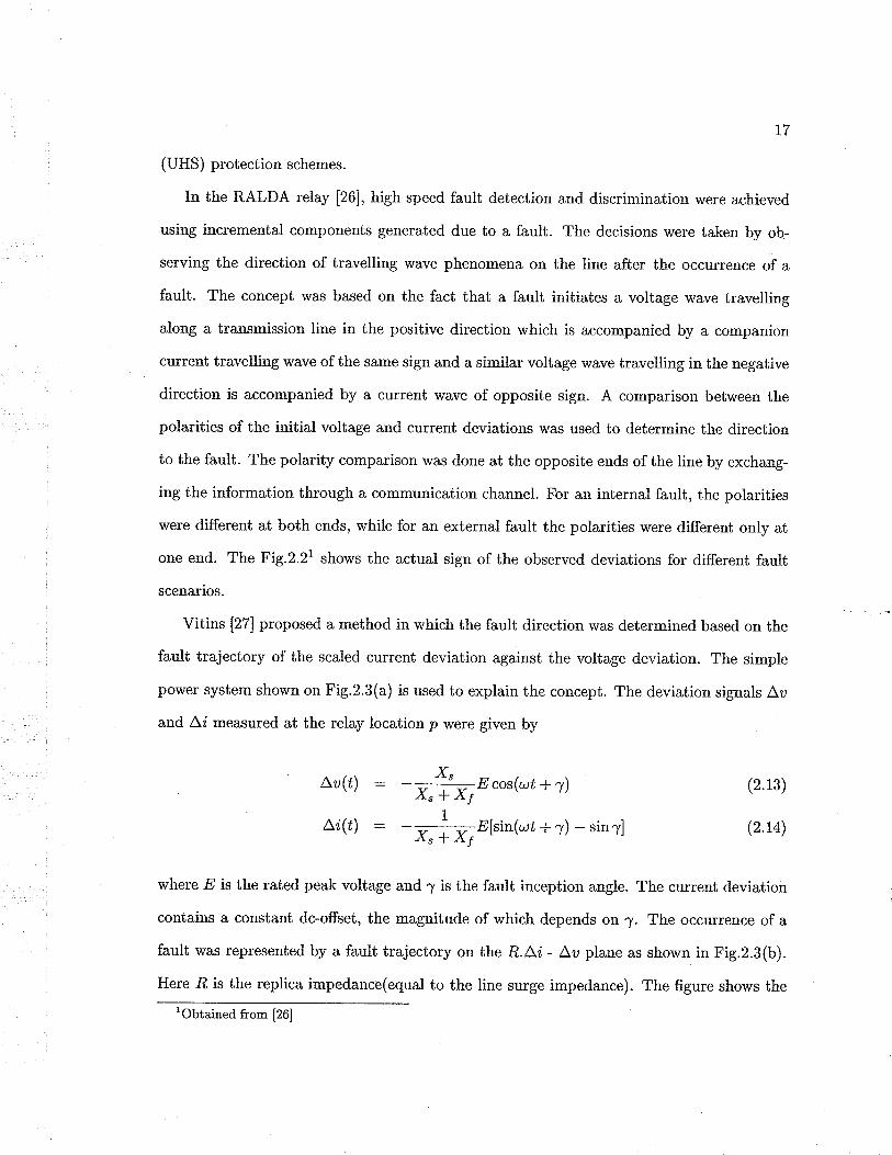
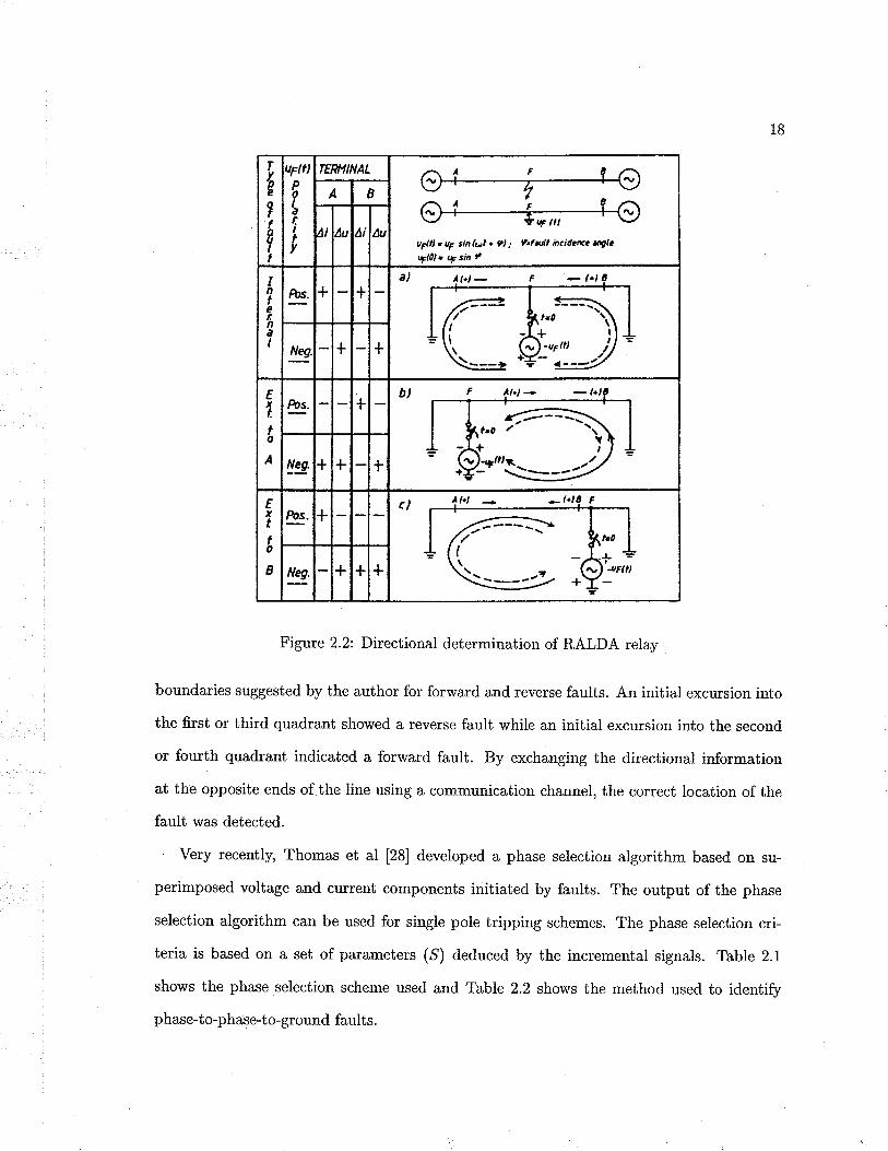
In the RALDA relay [26], high speed fauli detection and discrimination were achieved
using incremental components generated due to a fault. The decisions were taken by ob-
serving the direction of travelling wave phenomena on the line after the occurrence of a
fault. The concept was based on the fact that a fault initiates a voltage wave travelling
along a transmission line in the positive direction which is accompanied by a companion
current traveiling wave of the same sign and a similar voltage wave travelling in the negative
direction is accompanied by a current wave of opposite sign. A comparison between the
polarities of the initial voltage and current deviations was used to determine the direction
to the fault. The polarity comparison was done at the opposite ends of the line by exchang-
ing the information through a communication channel. For an internal fault, the polarities
were different at both ends, while for an external fault the polarities were different only at
one end. The Fig.2.21 shows the actual sign of the observed deviations for different fault
scenarios.
Vitins [27] proposed a method in which the fautt direction was determined based on the
fault trajectory of the scaled current deviation against the voltage deviation. The simple
power system shown on Fig.2.3(a) is used to explain the concept. The deviation signals Au
and Ai measured at the relay location p were given by
A,u(t\ : - X'
x, + xjø cos(r,,'ú * 7)
Ai(ú) : -n:Et[sin(a;ú+7) -sin.y]
(2.13)
(2.14)
where.Ð is the rated peak voltage and 7 is the fault inception angle. The current deviation
contains a constant dc-offset, the magnitude of which depends on .y. The occurrence of a
fault was represented by a fault trajectory on the R.Li - Au plane as shown in Fig.z.3(b).
Here .R is the replica impedance(equal to the line surge impedance). The figure shows thelObtained from [26]
'sf lneJ punor8-ot-aseqd-o1-aseqd
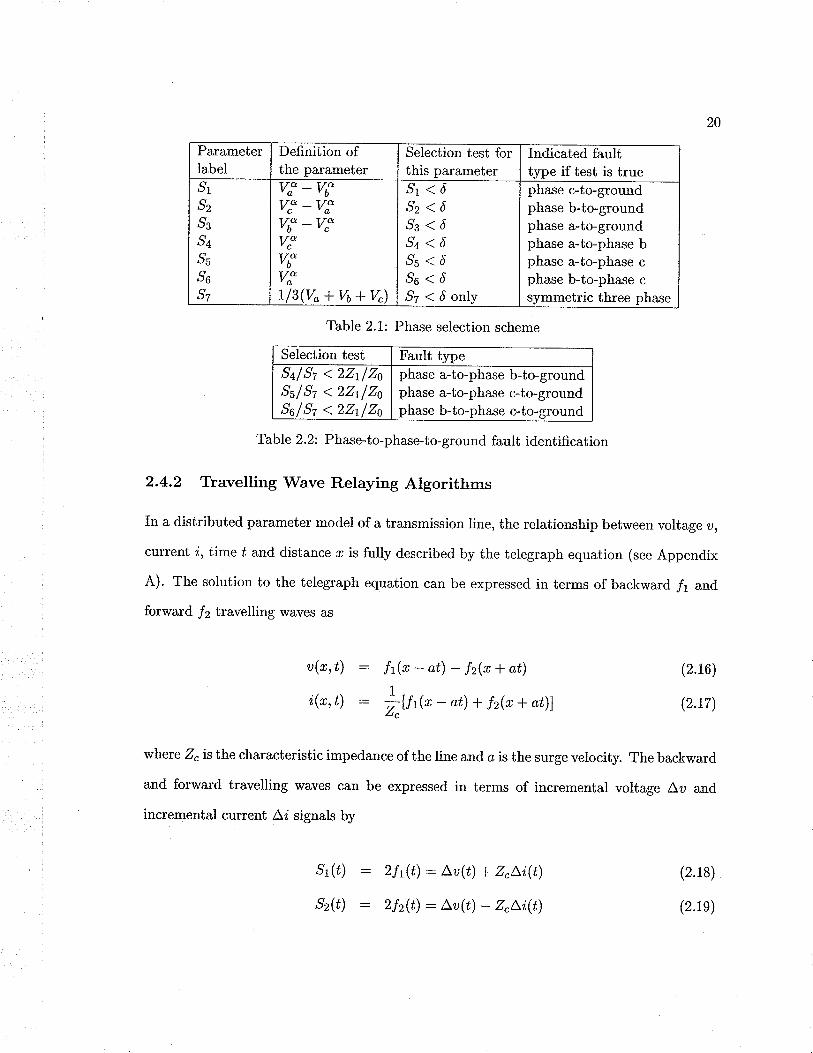
.,{¡¡1uap¡ o+ pasn poq?aru aq+ s/!ì,oqs z,'z oIqeJ, pue pasn aruaqls uorlcalas aseqd aql s^\or{s
T'U aIq"J 'qeuSrs lelualua¡cul aql fq pocnpap (g) sralauered ¡o las € uo pas"q sr €rral
-IrJ uollJalas aseqd aqJ 'sarnaqcs Surddr:1 a¡od e¡Burs roJ pasn oq uec urqlrroS¡e üorlcalos
aseqd arlî Jo 1nd1no ari¿ 's?In€J dq palerlrur sluauoduroJ lrrarrno pue a3e11o.r. pasodurrrad
-ns uo paseq urq1r.io31e uorlcalas asrqd e pado¡arrap [sz] I" la ssruoq¿ ,.{¡luaear ,{ra¡
'palra+aP s€^t ?In€J
arl+ Jo uoI+€col ?caJJoJ eq? (lauu€qc uorî?JrunururoJ B Susn aur¡ êqt Jo spua alrsoddo eq1 1e
uoll€IrrroJul leuolltarlp aq1 Sur8u€qcxa fg '1¡ne¡ pJ€lltroJ € pât€Jrpur luerpenb qlJnoJ ro
puocas aq? olur uorsrncxa lqÌIul u3 alrq/f\ ?ln€J asra^ãr € pa^\oqs luerpenb prqt ro tsrIl aq?
olul uolsmf,xa I€IlIuI uV 's+In€J asJa^al pu€ pJ€i\lJoJ JoJ Joq+n€ aq+ ,(q pa1sa88ns sarJepunoq
fela: yglyg Jo uorl€urrura+ap l€uor?Jarr¡l :¿.¿ arn8rg
¡rÉ
+
z o'l
+
+
+
BT
'6au
á ult t' 2 tO'+t¡ûtc tzttpttu ¿¡r*1.¿t : tò t ¿m¡ us ln . g¡ln
+
eoIIxl
+'sø
+
(q
+'6aN
+
+
V
oIT3
'sql
+ñ
++
n9
IeuIaIUI
'scc
!9n9
u
tç
TIIT
1od
lilln TVNtbktSt
I
i{8r
tv

19
o'
(b)
Figure 2.3: Fault trajectory and operating principle of vitins' algorithm
The aerial phase voltages, Vf, are given by
vf :vp -vo (2.15)
where Vo is the voltage of phase p and I/6 is the calculated ground mode voltage. The
threshold ô was set at 0.1 p.u. voltage. The test must be true for half a cycle of the power
frequency signals. The authors claimed that the proposed phase selection method is faster
than the traditional methods and valid over a broad frequency band.
(a)
Fault Trajectory
20
Table 2.1: Phase selection scheme
Selection test Fault typess,lsz <Zhlzssslsz <zhlzosa/sz <Zh/zo
phase a-to-phase b-to-groundphase a-to-phase c-to-groundphase b-to-phase c-to-ground
Table 2. 2: Phase-to-phase-to-ground fault identification
2.4.2 Tbavelling'Wave Relaying Algorithms
In a distributed parameter model of a transmission line, the relationship between voltage u,
current z, time ú and distance r is fully described by the telegraph equation (see Appendix
A). The solution to the telegraph equation can be expressed. in terms of backward /1 and
forward /2 travelling waves as
u(r,t)
i,(r,t)
Sr(¿)
Sz(t)
(2.16)
(2.17)
Ít(r-at)-f2(r+at)1
ltfr@-at)* fz(r+at)l
where Z"is t}ire characteristic impedance of the line and a is the surge velocity. The backward
and forward travelling waves can be expressed in terms of incremental voltage Au and
incremental current Ai signals by
zft(t): A'z(¿) + zcxi(t)
zfz(t): Lu(t) - z"Li(t)
(2.18)
(2.1e)
Parameterlabel
Definition ofthe parameter
Seleciion test forthis parameter
Indicated faulttvpe if test is true
,91
Sz
^93
Sa
5¡,96
Sz
V: _Vfv: -viVf _V:V:vb"viIlT(Va+Vu+V.)
Si<ôSz<6Ss<ôSa,<6,S5(ôSo<ô^97
( ô only
phase c-to-groundphase b-to-groundphase a-to-groundphase a-to-phase bphase a-to-phase cphase b-to-phase csymmetric three phase
2L
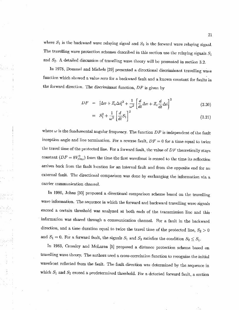
where ,9r is the backward wave relaying signal and ,92 is the forward wave relaying signal.
The travelling wave protection schemes described in this section use the relaying signals 51
and ^92, A detailed discussion of travelling rü/ave theory will be presented in section 3.2.
In 1978, Dommel and Michels [29] presented a directional discriminant travelling wave
function which showed a value zero for a backward fault and a known constant for faults in
the forward direction. The discriminant function, D.F' is given by
DF:
:
[Au + z"^i]2 . 3l*", + z"ftxrl'
s? + #l#',]'
(2.20)
(2.21,)
where a; is the fundamental angular frequency. The functio n D F is independeni of the fault
inception angle and line termination. For a reverse fault, DF :0 for a time equal to twice
the travel time of the protected line. For a forward fault, the value of D-F theoretically stays
constant (DF :ïV:^r) from the time the first wavefront is sensed to the time its reflection
arrives back from the fault location for an internal fault and from the opposite end for an
external fault. The directional comparison was done by exchanging the information via acarrier communication channel.
In 1980, Johns [30] proposed a directional comparison scheme based on the travelling
wave information. The sequence in which the forward and backward travelling wave signals
exceed a certain threshold was analyzed at both ends of the transmission line and this
information was shared through a communication channel. For a fault in the backward
direction, and a time duration equal to twice the travel time of the protected line, ,Sz ) 0
and 5r : 0. For a forwa¡d fault, the signals ,S1 and ^92 satisfies the condition ,S2 ( 51.
In 1983, Crossley and Mclaren [5] proposed a distance protection scheme based on
travelling wave theory. The authors used a cross-correlation function to recognize the initialwavefront reflected from the fault. The fault direction was determined by the sequence in
which '91 and ,S2 exceed a predetermined threshold. For a detected forward fault, a section
22
of the relaying signal ,92 representing the forward travelling wavefront was stored and cross-
correlated with subsequent sections of relaying signal 51. To obiain a better correlation
of .91 and ,S2, the mean values of the relaying signals were removed before calculating the
cross-co¡relation function. The cross-cor¡elation between the mean removed signals ,S1 and
,92 is given by
-^l-Qs,s,(m\.t) : ¡/ ÐISrQ'nt) - srzl.t,Sr(k\t + znAt) - -^911
k=I(2.22)
where ^9r and $- are the mean values of the signals 5i and ,S2 respectively. The cross-
correlation function shows a maximum value when the section 51 is similar to the stored
section ,S2. The time delay to reach this maximum corresponds to twice the distance between
the measuring point and the fault location.
Rajendra and Mclaren [31, 32] extended the techniques proposed in [5] to the protection
of teed circuits' The authors described several new travelling wave techniques to analyze
the faults on teed circuits. They suggested a polarity change criterion that enabled the local
end relay to disiinguish between a fault on the local branch and that of a fault on one of
the tee branches by sensing the polarity changes in the first and second backward travelling
wave in ^91. The polarity criterion was based on the fact that a fault on the local branch
will result in opposite changes in signal 51 whereas a fault on an adjacent branch will result
in identicai signal changes. The authors also suggested a method based on autocorrelation
function to classify faults between local and remote branches of a teed circuit. In this
method' the output section corresponding to the maximum of the cross-correlation function
is autocorrelated with sections of the entire cross-correlation function output. By doing so,
it was possible to determine the successive peaks of the cross-correlation output. It was
observed that the ratio of the time delays between successive peaks in the autocorrelation
output is approximately unity for a fault on the local branch whereas a low ratio is obtained
for an external fault or a remote branch.

23
In 1986, Mansour and Swift [33] presented a multi-microprocessor based faulted phase
selection and fault classification relay. An algorithm based on two discriminant functions
derived from the forward and backward travelling \¡/aves and their differentiations was used
to identify faulted phases. A table based on the transformation matrix used to decouple
the phase signals into their respective modal signals was proposed io identify different fault
scenarios. The backward and forward discriminant functions D6 and. DF respectively for
mode (k) were defined as
Dp:
Dp:
i'{*'l' . \fftsgl'
l'91'. ,4[#'r'1'
(2.23)
(2.24)
Here, the surge impedance Z" in (2.19) was replaced with the surge impedance associated
with mode (k) for each mode. The authors presented fault classification truth tables for
modal components found using Clarke, Wedepohl and Karrenbauer transformations.
Shehab-Eldin and Mclaren [3a] identified several problem areas associated with trav-
elling wave protection and suggested new techniques to improve the distance protection
scheme proposed by Crossley [5]. In Crossley's method, a reference signal representing the
first wavefront which leaves the relay location is stored and then a corresponding reflected
wavefront is found through correlation. The duration of this stored section is inversely
proportional to the wave transit time. The authors found that by using a fixed storage
duration, the protection scheme may not be able to detect either faults close to the relay (ifthe duration is long) or faults close to the remote bus bar (if the duration is short). They
suggested an improved method in which the final output is obtained by simple addition of
short and long window correlation outputs to form a composite correlation output. The
next improvement was suggested for close-up faults. For close-up faults, the travel time is
small and the relay may not be able to distinguish between the consecutive wavefronts. The
authors found that for close-up faults, the cross-correlation output is unidirectional and has
24
a very high value in magnitude. This situation was identified by comparing the average
value or the root mean square (RMS) value of the cross-correlation function instead of the
peak magnitude. The RMS value, d was evaluated over a time period equal to twice the
travel time, r of the protected line length. The value of d is given by
d- (2.25)
If d shows a value high and unidirectional, the disturbance is identified as a close-up fault.
When a fault occurs with an inception angle near or equal to zero, the relaying signals
become very small in magnitude and have a slow rate of rise. The authors described a
method to determine the inception angle, d for single line to ground faulis and suggested a
compensation method of relaying signal magnitudes. This modification did not affect ihe
cross-correlation shape, but increased ihe magnitude. The relaying signals were modified
AS
Sr^:.91[1+lcosál]
52*:,92[1 +lcosdl]
(2.26)
(2.27)
Christopoulos et aI [35] proposed a method based on travelling r,¡/aves to calculate the
distance to the fault. Initially, the magnitudes of the first voltage and current waves to
arrive at the relay location after a fault were measured. Flom the voltage and current,
apparent fault resistance was calculated. The magnitudes of subsequent voltage increments
and the time duration elapsed since the arrival of the first wave were then determined. For
each of the subsequent increments, the values were processed to find the apparent fault
resistance. When two values of fault resistance agreed, the elapsed time gave the distance
to the fault. This system could not detect faults with small inception angles. In addition,
the reflection coefficients of the busbar where the relay was located and the remote end
(ósr,s")2* l,*

25
busbar were assumed to be constant, which may not be true in a real system.
In a separaie publication, Christopoulos et aI [36] discussed the limitations in their
previous approach [35] and suggested several improvements. To systematically decide the
arrival of travelling waves at the relay location, the authors developed a method based on
cross-correlation algorithm used by Crossley and Mclaren [5]. The values of ihe cross-
correlation output were used to estimate the reflection coefficient at the fault location, and
hence the fault resistance. The fault resistance estimate was used to determine whether
the surge reflected from the fault point rather than from some other discontinuity on the
transmission line. The authors have also suggested methods to offset the errors caused by
varying reflection coefficients at the relay busbar.
A method for fauli location on transmission lines using the maximum tikelihood estimate
of the arrival times of reflected travelling waves was presented by Anceil and pahalawatte
[37]. The reflected travelling waves were expressed in terms of a set of incident rvr/aves which
were termed the basis signals s¿. A model of the measured fault transient y(k) was given
in the formI
a@):I",(r -r¿)a¿ k:7r...,Ni=l
where k is the sample index, s¿(k) is the basis signal, ø¿ is the associated reflection coefficient,
r¿ is the arrival time of the ith signal, 1 is the expected number of signals, and l/ is the
number of samples. Then (2.28) can be written in the matrix form
Y : S(r)a (2.2e)
(2.28)
26
where
v
s(")
s¿(r¿)
IaG),aQ),"' ,s(N)lt
["r("r), sz(rz),... , s¡(r¡)]
[r¿(t - r¿),s¿(2 - r¿),.. ., "¿(N - to)]'
forrozr"' ,alfr
frrr"r'' ' ' ,Ttfr
(2.30)
(2.31)
(2.32)
(2.33)
(2.34)
parameters ô,¡a¡ and
oi:
The maximum likelihood parameter method determines a set of
î¡a¡. The maximum likelihood estimate of ô is given by
ãuL : ls6)rv-L sQ)l-L s(+¡rv-ty (2.35)
The maximum likelihood estimate of î¡a¡ is the î which maximizes the function
J(î) : yrv-t s1+¡W(î)rvt s(î)l-1s(î)"v-ra - arv-ra (2.36)
Now, by estimating r, t]rie fault distance can be found. The authors claim that the
maximum likelihood method performs better than the correlation method, especially when
the faults have small inception angles. However, this meihod requires much more computa-
tional time than the correlation method and hence is difficult to implement as a real-time
application.
After 1995, many different algorithms based on travelling r,¡/ave signals could be found in
the literature, especially using wavelet transform, artificial intelligence methods and most
recently using high frequency current transients [38]. Some of them are described in section
2.5. only two other interesting developments are discussed in this section.
Liang et al [39] proposed a pattern recognition technique for travelling wave protection.
The method suggested ways to eliminate problems associated with ihe standard correlation
27
method suggested in [5]. First, instead of using the correlation method to identify the re-
flecting wavefronts, the authors suggested a pattern recognition technique based on nearest
neighbor method. Then they suggested a composite function which is based on both corre-
lation function and the nearest neighbor method to improve the performance. The nearest
neighbor method states that the pattern of an input vector is determined by the nearest
space distance between this vector and some reference vectors. The algorithm successively
measures the space distance between the stored section of the first forward travelling wave,
,92 and the section of backward travelling wave, ,91. When a surge with the same shape as
the reference signal arrives, the output of the space distance will give the minimum value.
Before calculating the space distance, the mean values are removed and the signals are
normalized.
,Sr(k) :
SzØ) :
lsr(r) - silmax(,S1)
ls2&) -E;1max(.92)
(2.37)
(2.38)
(2.3e)
(2.40)
by
Then the city block distance or Manhattan distance, d,¡7 of. the two signals is calculated
Ndm(k): r lsr(r) - sr(fr)l
le=L
The composite function, ó"(k) is a combination of d¡ø(k) and the correlation function
ó(k).
ó"(k):ñffidwhere the constant C1 avoids overflowing when the measured distance is zero. The maximum
{"(k) can be used to estimate the fault distance. The composite function improves accuracy
of the distance calculation.
In another paper [40], the same authors proposed an adaptive travelling wave protection
algorithm using two correlation functions. This adaptive method allows the protection

28
scheme to identify high impedance faults, which a travelling wave protection relay based
on standard correlation algorithm may fail to detect. According to the algorithm, for low
resistance faults, the fault distance is estimated from the standard correlation function,
while for high resistance faults, an auxiliary correlation function is uiilized. An adaptive
strategy guarantees that the signal with most prominent feature is taken as the template
to find the correlation, which improves the accuracy and the reliability of the algorithm.
2.5 Other Recent Developments
Power system protection had traditionally relied on the measurement of power frequency
component. Digital technology did allow some new techniques to be investigated. The
directional comparison schemes, travelling wave algorithms, and other transient based tech-
niques have become popular as ultra-high-speed protection methods. The adaptive protec-
tion schemes have been well accepted due to the improved stability they provide. Methods
that depend on artifici,al intelligence (AI) and wauelet transforms have shown improved
performance. This section very briefly discusses such recent developments.
Adaptive Protection
Adaptive protection is not a new concept. Time-delay overcurrent relays adapt their op-
erating time to fault current magnitude. Directional relays adapt io the direction of fault
current. These, however, are permanent characteristics of a relay or relay system and are
included as part of the original design or installation to perform a given function. The con-
cept of adaptive relaying is based on the fact thai many relay settings are dependent upon
assumed conditions on the power system. With complex interconnected power networks
today, it is difficult to assume some of these conditions. To faciliiate all possible scenarios
the protection scheme may have to handle, the actual protection settings in use are often
not optimal for any particular system state. If the relay needs to operate with an optimal
setting for a given condition of the power network, then the setting has to adapt itself to

29
the real-time system states as the system conditions change. Phadke and Horowúz laTl
mentioned, "In every phase of the development of a system's protection, a balance must
be struck between economy and performance, dependability and security, complexity and
simplicity, speed and accuracy, credible vs conceivable. The objective of providing adaptive
relay settings is to minimize compromises and allow relays to respond to actual system
conditions."
Rockefeller et al showed how the concepts of adaptive relaying can be introduced on
the existing power system lazl. Tbey showed the situations where adapiive relaying can be
used and their advantages:
o Adaptive system impedance model (permits calculation of fault-distribution): Im-
proved relaying reliability and possible avoidance of future line construction;
o Adaptive sequential instantaneous tripping (deiection of far-end breaker openings):
Faster back-up protection and possible elimination of the need for a second piloi
scheme;
o Adaptive multi-terminal relay coverage (accounts for changes in infeed ratios): Im-
proved zone 1 and zone 2 settings;
o Adaptive zorre 1 ground distance (accounts for large apparent impedance in fauli
resistance): Greater sensitivity to high resistance ground faults;
o Adaptive response to defective relaying equipment: Minimizes need for second pilot
scheme and need to take affected line out of service;
r Adaptive reclosing: Faster restoration following incorrect trips, reduced number of
unsuccessful reclosures, reduced shaft fatiguing;
o Variable breaker-failure timing (detects failure to interrupt): Improves back-up timing
margins and eliminates unneeded tripping of back-up breakers;
30
Adaptive last-resort islanding (system splitting to isolate generators with manageable
load levels): Improved probability of maintaining units in service to facilitate load
restoration;
Adaptive internal logic monitoring: Improved relaying reliability;
. Relay setting coordination checks (checks coverage and selectivity): Coordination
optimized, starting from existing power system conditions and minimizes operating
constraints.
They showed how the adaptive techniques can be implemented using the slow speed
responses of a SCADA system, in contrast to ihe high-speed channels used in pilot relaying
between interconnected transmission line terminals.
Horowitz et al presented an analysis of adaptive relaying concepts during the same time
[43]. They defined the adaptive concept as "Adaptive protection is a protection philosophy
which permits and seeks to make adjustments to protection functions in order to make them
more attuned to prevailing power system conditions". In their paper, they had investigated
the adaptive techniques applied to multi-terminal transmission line protection, relay set-
tings and automatic circuit breaker reclosing control. They showed how the adaptive relay
settings can be used in situations such as pre-fault load efiect, cold load pickup, source
impedance ratio, line charging and system asymmetries.
Protection Based on Artificial Intelligence
Artificial neural networks operate on the assumptions drawn on the behavior of biological
neural networks. An artificial neural network (ANN), or commonly known as artificial
intelligence (AI) provides a viable alternative to modelling nonlinear systems where it isdifficult to obtain a deterministic model to represent the system behavior. ANNs have
advantages as well as disadvantages: the implementation of the ANN does not require
complete understanding about the system behavior and hence can be used in extremely
3i
complex situations. However, training and testing of ANNs can take a long time and the
accuracy of the network depends on the size and the accuracy of the test set. The solutions
based on ANNs use different methods to increase performance in terms of speed of operation
and efficiency. ANNs have been used in various industries and have proved to be a vital tool
in applications related to power systems. One of the areas of power systems engineering
that gained more attention with use of ANNs is distance protection. A lot of applications
of ANNs can be found in relay literature, but we will only consider three applications for
this discussion.
Sidhu et al [44] presented an ANN based approach to determine the direction to the
fault. The directional discrimination was achieved through a multi-layer feed-forward neural
network. The paper discusses important issues related to the implementation of the ANN:
preparation of suitable training data, selection of a suitable ANN structure, training of the
ANN, and evaluation of the trained network using test patterns. The data for training was
obtained by simulating the power system on EMTDC. During the selection process of ANN
structure, number of layers, transfer function, number of neurons and number of inputs and
outputs had to be chosen appropriately to identify all fault conditions.
Coury and Jorge [45] showed how the magnitudes of the three phase voltage and current
phasors can be utilized in an ANN based protection relay to achieve fast and precise opera-
tion under different fault conditions and changes in the network. The neural network they
used was based on the backpropagation algorithm. The backpropagation algorithm works
by adjusting the weights which are connected in successive layers of multi-layer perceptrons.
The ANN based approach made it possible to extend the zone 1 reach of distance relays,
hence improving the security.
Venkatesan and Balamurugan [46] developed a real-time fault detector for the distance
protection application based on artiûcial neural networks. The paper describes their ap-
proach to data analysis, feature extraction, software design and simulation, quantization,
performance analysis, hardware design and implementation of the ANN based relay. For

32
the softwa¡e design an ANN simulator has been developed using the C++ programming
language instead of using the commercially available simulators. The hardware implementa-
tion has been done using a single chip with both the preprocessors and the neural processor
on the same chip. ifhe relay could detect faults in the transmission line within one third of
a power cycle from the inception of fault.
'Wavelet Transform Methods
In recent years, researchers have developed powerful wavelet techniques for the multiscale
representation and analysis of signals. These new methods differ from the traditional Fourier
techniques' The Wavelet Tbansform (WT) is of interest for the analysis of non-stationary
signals. It provides an alternative to the classical Short-Time Fourier tansform (STFT)
or Gabor transform. In contrast to the STFT, which uses a single analysis window, the
WT uses short windows at high frequencies and long wind.ows at low frequencies. Wavelets
localize the information in the time-frequency plane; in particular, they are capable of
trading one type of resolution for another, which makes them especially suitable for the
analysis of non-stationary signals [42].
The wavelet transform is an operation that transforms a function by integrating it with
modified versions of some kernel function [48]. The kernel function is called the mother
wavelet, and the modificaiions are translations and compressions of the mother wavelet.
For a function to be a mother wavelet, it must be ad,missi,ble. A function g e L2(R) is
admissible if
.,=l:ff,,.* (2.41)
where G(ø) is the Fourier transform of g(ú), L2@) is the set of all square integrable or
finite energy signals, and .R denotes the real numbers. The constant c, is the ad,mi,ssi,bility
constønt of the function g(ú), and the requirement that it is finiie allows for inversion of the
wavelet transform. Any admissible function can be a mother wavelet. For a given function

oo,f .)
g(ú), the rnother uauelet of the transform is assumed to be admissible. Wavelet transform
can be in analog domain (Continuous Wavelet TÌansform, CWT) or digital domain (Discrete
Wavelet Tlansform, DWT). The mother wavelets can be orthogonal or non-orthogonal. In
much of the wavelet transform literature, dyadic orthogonal mother wavelets are chosen as
the mother *arrelôt.
The CWT of a functior f (t) with respect to the wavelet function tþ(t) is given by
W,¡f (a,b): f (t)ú.(:lldt
Y,''tt.Fffl
+"1: (2.42\
where ¿ and ö are the scaling (dilation) and translation (time shift) constants respectivety.
The DWT as applied to sampled waveform /(k) is given by
W,¡f (m,n): (2.43)
where the parameters ø and b in (2.a\ are replaced by oT arrd kaff, k and rn being integer
variables.
One important area of application where wavelet transform has been found to be relevant
is power engineering. Lee et at [a9] did a literature survey to find application of wavelets
in power systems. They found that wavelet transform can be readily applied to power
distu¡bance detection and localization, power disturbance data compression and storage,
power disturbance identification and classification, power devices protection and power
disturbance network/system analysis. Robertson et al [50] showed how wavelet transform
can be used to identify the transients on the power system. In this section, we will discuss
few applications of wavelet transform in transmission line protection schemes.
Magnago and Abur showed how the high frequency travelling waves can be identified
with the aid of wavelet transform and how that information can be used to estimate the
distance to the fault [51]. Two different approaches to estimate the fault location have been
attempied. fn one method, fault transients at the two ends of the transmission line are
I--..-:t/"7

34
identified through synchronized recording of transient signals. The recordings are synchro-
nized using a GPS meihod. Time difference between the arrival of the wavefronts at the
two ends are used to estimate the distance. In the second method only the mea.surements
at one end are used for the protection. The arrival of the consecutive wavefronts are used
to estimate the distance to the fault. Different algorithms are used in the case of grounded
or ungrounded faults.
Shang et al [52] used wavelet transform to develop a high-speed protection algorithm for
transmission line protection. The wavelet modulus maxima (\MMM) was used as a criterion
to detect fauli conditions (the absolute local maximum values of the wavelet transform of
ihe signal are called wavelet modulus maxima). The WMM must satisfy the condition given
by
lW^""r(t)l l ksd (2.44)
Here, W*o"r(t) is ihe \MMM of signal r(t), k is a constant, s is scale and a is the
Lipschitz exponent. The polarity of the WMM associated with consecutive wavefronts
is used for the fault identification. Using this method, ii is possible to identify special
situations such as switching onto unloaded lines and onto faulted lines.
Yibin ei aI [53] proposed a way to use wavelet transform to extract the fundamental
frequency components of the three phase signals and use the fundamental components
to calculate the fault location. The wavelet method has been compared with the results
obtained by using the standard Fourier transform methods.
Wai and Yibin [54] investigated a method to use wavelets for high impedance fault
identification. They describe how high impedance faults and capacitor bank switching
can be classified using wavelet analysis fiIter banks. The filter banks are implemented as
cascaded quadrature mirror fiIters. The high impedance faults are modelled in an improved
method to yield better simulation results. The wavelet transform of the transient signals
showed different characteristics under high impedance faults and capacitor switching.
tt
Wide Area Protection
In the early days, the primary function of protective relays was to simply protect the power
system components. However, with the advent of the microprocessor relays, it became ob-
vious that microprocessor relays can provide both protection and measurement functions.
The ability of new microprocessor relays to communicate with each other and the avail-
ability of broadband communication links allowed them to share information thai could be
used for supervisory control and protection purposes. Because of the advancing technology
of protective relays and their communication capabilities, the new relays are called Intelli-
gent Electronic Devices (IED) [55]. The high-speed communication links allowed relays to
quickly update their status to each other or to a central control station. This technology
advancements and the time synchronizing capability of GPS are used in the new wide area
backup protection algorithms. Wide area backup protection schemes are considered a pos-
sible solution for preventing blackout situations. We will briefly discuss two methods used
in wide area protection.
Serizawa ei aI [56] proposed a wide area current differential backup protection scheme.
The current differential scheme provides a higher selectivity than the conventional backup
protection employing distance relays. The proposed system configuration utilized ATM
transmission networks and time synchronous systems. For the current differential protection
scheme, the current measurements of each busbar and transmission lines and transformers
connected to that bus bar are consid.ered. For the backup protection of long transmission
Iines GPS synchronized current measurements were taken at the ends of the line.
Tan et al [57] proposed a wide area backup protection scheme that could prevent cascad-
ing outages in power systems. The backup protection scheme prevents cascaded tripping in
two ways: 1) It determines the precise location of a fault so that only the circuit breakers
necessary to isolate the fault are tripped and 2) It avoids unnecessary trips, due to hidden
failure or overloading, by blocking the trip signals ofconventional backup protection relays.
To prevent cascading trips, a wide area backup protection expert system (BPES) is used.

36
BPES is a wide area communication network based protection system designed to protect a
region of the network by providing seiective and secure backups. The BPES operates in two
modes: normal and emergency mode. During normal operation, the BPES monitors the
open/closed states of circuit breakers and the operational response of conventional protec-
tion relays on the network. It changes to the emergency mode when a fault is detected and
decides ihe besi way to isolate the fault if the main protection has failed. The BPES may
block a conventional backup protection relay if necessary. The paper extensively discusses
the implementation details, the possible fault scenarios, and how the BPES can be used for
preventive control of wide area blackouts.
Chapter 3
Theoretical Aspects
3.1 Introduction
The hybrid relay utilizes both travelling wave information derived from the high frequency
transient signals and the impedance calculated from the fundamental components of the
voltage and current signals. Before understanding how the hybrid relay works, it is impor-
tant to have an idea about basic principles behind the travelling wave protection as well as
impedance measurement scheme. In this chapter, we introduce theory behind these algo-
rithms. The theory associated with the travelling wave protection will be discussed first.
In order to simplify the explanation, a single phase lossless line will be used to introduce
the theory. This explanation will then be extended to a three phase system. The travelling
wave theory will be followed by an introduction to the impedance algorithm. Finally, we
will discuss how the two algorithms are combined and the operating principle of the hybrid
algorithm.
.Jt
38
3.2 Theory of Tbavelling 'Wave Protection
3.2.L Tbansient'Waves
Faults which occur on a high voltage transmission line at an instant of a non-zero voltage
will cause the pre-fault line charge to rapidly discharge. This can generate heavy surges on
the transmission line which will propagate as waves. These v/aves will travel close to the
speed of lighi along both directions of the transmission line from the fault point and reflect
at discontinuities along the line, including the fault point itself. The repeated reflection
of these surges or waves produces decaying high frequency voltage and current transients.
Each wave is a composite of frequencies, ranging from a few kilohertz to several megahertz,
having a fast rising front and a slower decaying tail [58]. These composite v¡aves have a
characteristic impedance that will depend on the line parameters. The waves continue to
exist until they are damped out and a nerrr/ power system equilibrium is reached. In an extra
high voltage (EHV) transmission line, where the line length and the system capacitance
are large, these transients become significant, specially with small resistance in the faulted
network. These transient signals, which will be identified as travelling 'ù/aves, can be utilized
to detect faults in power transmission lines.
3.2.2 Basic Principles Developed on a Single Phase Model
The principles developed will be for lossless single-phase transmission lines. The lossy case
has to be considered separately. However on EHV transmission lines, the effects of resistance
in the fault loop is minimal and may be neglected in the derivations.
Principle of Superposition
The faulted network can be described using the principle of superposition as shown in
Fig.3.1. The voltage and current signals are measured at the relay location -R. Consider a
line to ground fault at point F in Fig.3.1 (a) . The inception of a fault in the power system will

39
cause the post-fault voltage u¡ and current i¿ at the relay location R to deviate from the
steady state pre-fault voltage u! and current zþ. The deviation signals or the incremental
components can be considered to be generated by switching on a fictitious voltage source
at the fault point with a voltage equal in magnitude and opposite in sign to the pre-fault
voltage at the fault point, and with all other sources suppressed.
The superposition of the pre-fault signals in Fig.3.l(b) and the deviation signals in
Fig.3.1(c) produce the post-fault signals. We then have
UR(T)
in(t)
u'*(t) t Lup(t)
i'R(t) + LiR(t)
(3.1)
(3.2)
where Au¿(t) and Az¿(ú) are the fault generated voltage and current deviations from the
steady state pre-fault values at the relay location respectively. The deviation signals Au¿(t)
and Az¿(ú) are readily obtained from the measured post-fault voltage up and current i4
signals by subtracting the sinusoidal pre-fault steady state voltage uþ and current ii com-
ponents. These superimposed quantities are used in the travelling wave relaying algorithms,
as used by others in the past [5],[26]-136]
The voltage deviation Au¿ will depend on the amplitude of the voltage at the fault
location at ihe instant of the fault, impedance values of the sources and line and the fault
resistance. The magnitude of the initial voltage deviation is maximal for faults occurring
at the moment of a voltage maximum, while it is zero for faults occurring during a voltage
zero. The current deviation A'd¿ contains an exponentially decaying component commonly
known as a constant dc-offset, the magnitude of which depends on the fault inception angle.
The exponential component is maximal for faults incepted at a voltage zero and zero for
faults occurring at a voltage maximum. The resistance in the fault loop will cause the offset
in the current signal to decay. These resistances will further reduce the magnitude of both
voltage and current deviations.
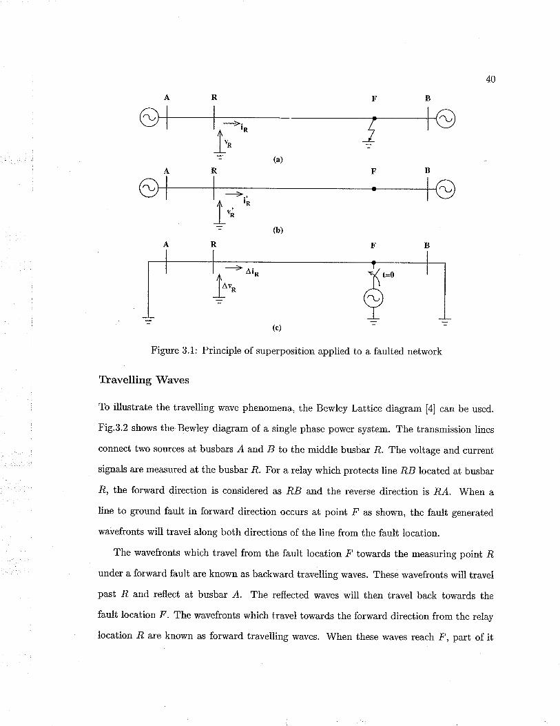
40
+i*
=R
Figure 3.1: Principle of superposition applied to a fauited network
Travelling 'Waves
To illustraie the travelling wave phenomena, the Bewley Lattice diagram [4] can be used.
Fig'3.2 shows the Bewley diagram of a single phase power system. The transmission lines
connect two sources at busbars ,4. and B to the middle busbar ,R. The voltage and current
signals are measured at the busbar ,R. For a relay which protects line ,RB located at busbar
-R, the forward direction is considered as J?B and the reverse direction is ,Rr4.. When a
line to ground fault in forward direction occurs at point .F' as shown, the fault generated
wavefronts will travel along both directions of the line from the fault location.
The wavefronts which travel from the fault location tr' towards the measuring point ,R
under a forward fault are known as backward travelling waves. These wavefronts will travel
past .R and reflect at busbar -4. The reflected waves will then travel back towards the
fault location tr'. The wavefronts which travel towards the forwa¡d direction from the relay
location r? are known as forward travelling v¡aves. When these waves reach -F, part of it

4I
will reflect from the fault point F while the remaining part propagates towards the busbar
B. These two components are known as reflected and transmitted waves, respectively.
The magnitude of the reflected and transmitted wavefronts will depend on the fault
impedance and ihe impedance of the transmission line. The reflected wave "o-porr"rrt.
wili travel back towards .R again. The wavefronts which travel towards the busbar B from
the fault location ,F will reflect from busbar B and reach -F again. Part of them will be
transmitted towards -R and the other part will be reflected back towards busbar B. The
wavefronts will continue to propagate and reflect in this manner until they are damped out.
| ---
Figure 3.2: Bewley lattice diagram of wavefronts generated by a fault
The voltage and current signals on a transmission line can be considered to be a sum-
mation of a backward travelling ìñ¡ave .F1 and a forward travelling wave F2 (see Appendix
A). These waves propagate with a constant amplitude at a velocity slightly less than the
speed of light. The amplitude and the shape of these waves may change in a lossy line. The

42
general solution of the wave equation is given by
u(r,t)
i,(r,t)
h(r-at)-F2(r*at)1
4[r(r-at)*F2@+at)]
fí*-at)-f2(r+at)1
llft@-at)+Íz(r+at)l
(3.3)
(3.4)
where Z" is the surge impedance of the line and '¿' is the propagation velocity of the waves
in the line.
If only the incremental components are considered as in 3.1 and 3.2, the fault generated
voltage and current deviations can be expressed as
Lu(r,t)
Li.(r,t)
Lu(r,t) + Z..Li(r,,t)
Au(r,t) - Z".Li.(r,t)
2.ft@-at):5,
-2.Íz(r*at):5,
(3.5)
(3.6)
(3.7)
(3.8)
where /1 and f2 are the backward and forward travelling waves calculated from the incre-
mental components of the voltage and current signals. Hence from (3.5) and (3.6), it can
be shown that
The signals ,9i and .92 represent the backward and forward travelling waves and will be
used as the backward and. forward relaying signals in the travelling wave algorithm.
Forward Fault
Fig.3.3 shows the propagation and reflection of waves generated due to a forward fault
on a transmission line. The wavefronts reflect at the fault point F', and the busbars L
and B. The voltage and current signals are measured at busbar J?. In order to derive
the mathematical equations, the measured signals are considered to be the incremental

43
components as described in (3.3) and (3.4).
The first backward travelling wave /1 reaches R at rl seconds after the instant of fault
inception and will reach busbar A at time r. The wave /1 reflects from busbar .4 and
travels towards the fault location passing ,R at time 12. When the forward travelling wave
/2 reaches.F at time 2r,part of it will reflect from.F while the remaining part propagates
towards the busbar B. The part of the travelling wave f2 that reflected from F (shown as
/r") will reach the busba¡ -R at time 13 and reflect from busbar A at time Br.
ARFB
Figure 3.3: The propagation and reflection of wavefronts in a forward fault
As already mentioned, a fault can be described as introducing a voltage source equal in
magnitude and opposite in sign at the fault point, at the time of the fault. If the pre-fault
steady state voltage is given by Vpsin(r,,rf + d), the voltage deviation Aup due to the fault
is then
Aup(ú) : -u'p,(t) - -Vnsin(øú + /) (3.e)
flÍlt
where, uþ is the pre-fault steady state voltage at point F. The voltage waveform is assumed

44
to be sinusoidal with a peak value Vo : t/ÍV"*r.
If the fault occurs at time ú, considering the wave propagation times shown in Fig.3.3,
the voltage and current deviations seen at the relay point -B can be combined to obiain the
foilowing relationships:
Lup(t) 1- Z".Lipp(t) : A,up(t + rr) + Z".Lin(t + rt)
Au¡(ú) - Z..Li,Bp(t) : Auf'(t+ "r)
* Z..Lip(t + r)
(3.10)
(3.11)
where Ae¿p is the deviation in current with current measurement taken as positive in the
direction from relay point rR to fault location,F'. 11 represents the travel time for the waves
from -F to ,R.
But at time 4, the forward travelling wave f2 is equal to zero at the relaying poini.
Hence from (3.8) and (3.11)
Lu¡"(t+11) - Z..A,i,p(t*1) :g
The condition in (3.9) combined with (3.12) yields
(3.12)
Li,pp(t) : Aur(¿) _ -Vosin(ut -t ó)zc
Using the above results, (3.i0) can be solved to give
Aur'(t + 11) + Z".Lí. ¡(t f 1) : -2Vr sin(at + ó)
By introducing a time shift, from (3.7) we thus obtain
(3.i3)
l{t + rt) : -2Vpsin(øú + @)
f{t) : -2Vosin(ut - urt -l ó) (3.14)

45
for 1 ( t 12r*r1. The backward travelling u¡ave /1 is initially independent of the terminal
conditions. If ri is small compared to the period of the 60Hz signal, for a lossless line, it ispossible to approximate fl of (3.1a) to have a constant value of
/r(¿) = -2Vosin(þ) (3.15)
for the time period 11 1t 12r * r1.
When the backward travelling wave arrives at the line terminal, the wavefront will
reflect and travel towards the fault again. This reflected wave will have a reduced amplitude
compared to that of the incoming wave depending on the terminal conditions. The reflected
wave will be of the "form"
fz: €ft (3.16)
for 12 1 t { 2r * 12 where ( is the reflection coefficient of the termination. Hence from
(3.15), the forward wave front of /2 will have the *shape"
Íz(t) = (zVosin(þ) (3.17)
The shape of this reflected waveform will mainly depend on the terminal characteristics.
For example on a lossless line with surge impedance Zc, if an incoming wave of the shape
given in (3.15) reflects from a source consisting of a pure inductance .L",
Íz(t) : - ze-t*t'2.1 (3.18 )
for 12 < t 12r + 72. The high frequency steep signal will be reflected immediately and the
low frequency signals will reflect with an exponential decay.
Izo sin(/) lr

46
AF R
Figure 3.4: \Mave propagation for a reverse fault
Reverse Fault
For a reverse fault with respect to the relaying point .8, as in Fig.3.4, the relay first sees
the forward travelling wave f2. The travelling waves will propagate past .R along the line
and reflect at the remote busbar B. The first forward wavefront /2 reaches -R at time 11.
This will reach busbar B at time r. The wavefront f2 will reflect from busbar B and travel
towards the relay location R at time 12.
If the pre-fault steady state voltage is given by I/o sin(øt+ ó), the voltage deviation Ar'¡
due to the fault then is
Aup(t) - -Vnsin(øú+/) (3.1e)
If ihe fault occurs at time f, considering the \¡yave propagation times shown in Fig.3.4,
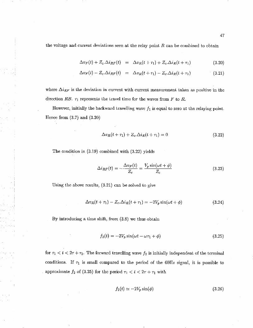
47
the voltage and current deviations seen at the relay point Ê can be combined to obtain
Aup(ú) -f Z¿.Lipp(t) : Lu¡'(t + rr) + Z".A,i,p(t + 11)
Aup(t) - Z..Li,RF(t) : A.up(t+"t) - Z".A,ip(t*11)
where Ai¿p is the deviation in current with current measurement taken as positive in the
direction RB. 11 represents the travel time for the waves from F to ,R.
However, initially the backward travelling wave /1 is equal to zero at the relaying point.
Hence from (3.7) and (3.20)
A,up(t+l.1) + Z..L.i,p(t*11) :g
The condition in (3.19) combined wiih (3.22) yields
(3.22)
(3.20)
(3.21)
(3.23)^;__i,+\ _ Aup(ú) _Vosin(at* Q)
ÀLùùr''t: --'Lt ' Zc Z"
Using the above results, (3.21) can be solved to give
Lu¡'(t*rr) - Z..Aip(t*q) : -2Vosin(wt*þ)
By introducing a time shift, from (3.8) we thus obtain
(3.24)
fz(t) : *ZVosin(ut - urt * ó) (3.25)
for rr ( t < 2r + ?-1. The forward travelling wave f2 is initially independent of the terminal
conditions. If 11 is small compared to the period of the 60Hz signal, it is possible to
approximate f2 of (3.25) for the period 11 1t < 2r * 11 with
Íz(t) = -2Vosin(þ) (3.26)
48
3.2.3 Three Phase Systems
Background
On a three phase transmission system, when a fault occurs on one cond.uctor, transient
cu¡rents will be induced in the healihy conductors due to the mutual coupling between
them. The mutual elements of the surge impedance matrix allow the travelling waves to
couple across ihe phases. The waves induced on sound phases from the faulted phase travel
between the two ends of the line and subsequently interact with the waves on the faulted
phase [59]. This could distort the waves on all three phases. Due to the coupling effect, the
set of equations describing the propagation of waves on each phase become interdependent.
According to the theory of natural modes [60], using modal transformation a three-phase
coupled line can be decomposed into three independent modes of propagation or three
single-phase lines (see Appendix B). The travelling wave theory applied for a single phase
circuit can be readily applied to the independent modes separately to analyze the faults
and hence to analyze a three phase system.
Modal Tlansformation
In developing the travelling wave theory for the single-phase system, the line was assumed
to be ideal (no-loss). In a lossless line, the current and voltage waves are subject to the same
attenuation and have the same velocity at all the frequencies. Attenuation and distortion
are due to resistive elements and the effect of frequency dependent elements in the network.
The frequency dependent, nonuniform distribution of the ground currents due to the earth
conductivity has io be considered when dealing with an actual system. Appendix A discusses
the formulation of travelling wave signals for a lossy line and Appendix B deals with the
voltage current relationship in a three phase system and how the three phase system can
be transformed into three independent single phase systems or modes.
49
The relationship between the three phase signals and modal components for voltage and
current signals is given by
[t'(t)1 : [s][u{*)1r¡1
[,(¿)] : lq!@@l
where [S] and [Q] are ihe voitage and current modal transformation matrices respectively.
¡u(-)1t¡1 and [z(-)(t¡] are the modal voltage and current matrices. The inverse relationship
is given by
¡u('") 1i¡1 : [^9j-1[r(¿)]
li(r¿) (¿)l : [Q]-1 þ(¿)l
(3.27)
(3.28)
The modal signals are assumed to have a single propagation velocity for each mode.
The aerial modes will not cause a significant error over the frequency range considered and
hence can be assumed frequency independent. However, for a single phase to earth fault,
the dominant mode of propagation is the earth mode (model). The earth mode parameters
depend on the earth resistivity and may cause significani variations in the propagation
velocity [61]. The ground mode has lower velocity and greater attenuation and distortion
than the aerial modes (mode2 and modeS) because of the frequency dependence of their
parameters. The velocity of waves in aerial modes is close to the speed of light. The
veiocity and attenuation of the aerial modes for a fuliy transposed single circuit three phase
system are identical. In the studies reported in this thesis, a fully transposed transmission
system is assumed and the modal transformation matrices mentioned in Appendix B are
used for the transformation like many others did [5, 31, 34, 33, 35]. Since the earth mode is
frequency dependent and the velocity varies with the frequency, the earth mode was found
to be difficult to use for the fault analysis. Hence for deriving the relaying signals, the aerial
mode 2 will be used.
Travelling 'Waves in a Three Phase Systern
To derive the travelling wave signals in a three phase system, the modal components of
the incremental voltage and current are used. The incremental voltage, Au and current,
Az components are calculated separately for each phase to find the deviation from steady
state components. The modal components of the incremental voitage and current signals
are found by using a modal transformation matrix described in Appendix B. For example,
if the Clarke transformation is considered,
(3.2e)
llll l:*l: ;;lLîÍ land
Ll,lll l:*l: ; ;llll I ""'The modal voltage components Au(-) and Ai(-) for each mode nL can- be used to
derive the forward and backward waves for individual modes of propagation. The backward
relaying signal ^9{-) fot mode ræ is given by
sÍ-) : A"9) + z[ù 6¿('")
and the forward relaying signal Sf) ø, mode rn is given by
(3.31)
St*) : L"9) - z[ù 6¿f') (3.32)
where Lug') and Azf) are the incremental voltage and current quantities of mode rn at
relay location R. Z! is the surge imFedance for mode rn.
51
The wave components ,Sfl and Sf can be used in the same way as in a single phase
transmission line model described in section 3.2.2. Here onwards in this thesis, the notation
^9r and .92 will indicate the backward and forward relaying signals that belong to the aerial
mode 2.
3.2.4 Fault Direction
Tlavelling'Wave F\rnctions
The travelling wave functions 5r and ,92 calculated using incremental components of the
voltage and current signals must ideally have zero magnitude when the power system op-
erates under steady state conditions. Even with ihe numerical errors associated with the
calculations in practice, they show extremely low values. However, when a fault occurs in the
system, the voltage and current signals deviate significantly from their steady state values
and hence ^9r and ,52 will show large magnitudes. A change in magnitude of the travelling
wave signals (from near-zero values) could indicate a disturbance on the line. Depending on
the fault direction and reiay location, the sequence in which the signals ,9r and 52 become
non-zero can vary. The direction of the fault can be determined by the sequence in which
,5i and .92 exceed a predetermined threshold. ff 52 erceed,s a certa,i'n threshold before 51,
then the fault i,s i,n the backward d'i,rect'i,on, else the fault i,s in the forward, direction.
Discriminant Functions
The backward and forward travelling wave functions Si and ,92 are dependent on the fault
inception angle @. In an unlikely situation when a fault occurs near a voltage zero (ie. fault
inception angle is close to zero), the signals ,91 and Sz will have small magnitudes. Under
such conditions, it might be difficult to detect a fault only using the 51 and ,92 signals.
Identification of fault conditions and direction can be improved by using a method that will
be independeni of the fault inception angle. To improve the reliability in fault detection, a
di'scrirninant functi,on which does not depend on @ can be used. The discriminant functions
52
are calculated using the travelling wave functions and their differentiations [29]. The back-
ward discriminant function D6 and forward discriminant function Dp for a single phase
system are given bg
DB : (LVa+ Z".A,Ip)2 +
DF: (LVa- Z..A,I¡)2 +
(3.33)
(3.34)
The discriminant functions are initially termination independent and the performance
of the functions do not depend on the fault inception angle. D6 a.nid Dp a,re zero for
a healthy line and show very high values in case of a fault. The highly decisive nature of
these functions can be utilized to classify forward and reverse faults. If D e erceeds a certa,i,n
threshold ualue before D6, i,t is a backuard fault, otherwise i,t i,s a forward fault.
3.2.5 Determination of Fault Location
The travelling wave relaying signals 51 and 52 carr be used to determine the direction of
the fault. The relay is set up to operate on a forward fault. However, the relay must
be able to determine whether the disturbance occurred within its zone of protection. To
determine whether the fault is within the zone of protection, the distance to the fault can be
used. The distance to the fault is evaluated using the time difference between an identified
forward wavefront at the relay point and the corresponding wavefront reflected from the
fault point. To match the two wavefronts correlation techniques are used. The correlation
techniques provide a method to distinguish the required wavefront from other surges on
the line. Recently, there has been an increasing interest in applying wavelet transform
methods to detect transients. However, it is difficult to find a clear method of choosing a
suitable mother wavelet which could identify different fault conditions. Due to the robust
and simple implementation of the correlation algorithm, a cross-correlation function will be
used to calculate the distance to the fault in the proposed method.
#l#^^+ z. ^IR)]2
,L,l*^""- z*^Iù]

53
\Mhen a fault occurs, the fault generated wavefronts will propagate along both directions
of the line, as shown in Fig.3.3. The first wavefront /1 reaches the relay location at time
1. Since signal ,92 is still low at this time, a forward fault is detected. When the signal
52 goes above a certain threshold at time T2, a forward wavefront is detected at l?. Once a
forward fault is detected, the relay starts storing the forward travelling wave signal ^92. This
wavefront ,Sz is stored in a window of Iy' samples as a reference signal. The storage time
is selected so that the stored signal will contain both pre-fault and post-fault information.
The wavefront f2 will reflect at the fault point and a portion of the wavefront will return
to the relay location at time 13. The reflected wave front is identified by matching the
backward relaying signal ^9r to the stored signal92. To identify the correct wavefront, the
cross-correlation is found between the stored and returning signals [5]. The time 13 at which
the reflected wave ,91 matches the stored signal .92 is estimated by finding the instant at
which the cross-correlation of the two signals shows a peak value.
The distance to the fault can be calculated by,
{DÍ: (3.35)
where ¿ is the velocity of propagation of waves on the line. If the distance r¡ is less than
the line length, the fault falls within the protection zone of the relay.
3.2.6 Correlation Techniques
Correlation is a measure of a linear relationship between two variables. Correlation can be
readily applied to both random variables and deterministic functions. Correlation methods
are widely used in applications where a signal has to be detected in the presence of noise
(see Appendix C). The correlation technique can be applied to both analog and discrete
signals.
Ts-T22.o

54
Correlation in the Analog Domain
The purpose of autocorrelation is to analyze the relation between the values of the same
random process at different times. The autocorrelation function of a time invariant signal
r(ú) is defined as
(3.36)
This reveals the presence of a recrrrence in a random signal. For a periodic signal, the
autocorrelation function is also periodic. R"(r) is an even function;
R"(r): R,(-r) (3.37)
The auto-covariance Õ'(") of signal z(f) shows the correlation of the signal r(t) at
different times, if the signal is made to be of zero mean.
Õ"(") : R,(r) -n2 (3.38)
The value of the autocorrelation function without a dela¡ Ë"(0), gives the time average
of the square of each value of ø, known a,s mean-square of z.
R,(,): ÆL + l,' r(t).t(t * r)dt
R"(o) : + Ir' n2çt¡ at (3.3e)
The mean square value of the signal can be used to normalize the autocorrelation result
since
Ã"(0) > R"(r) (3.40)
The cross-correlation function provides the relation between two signals which may be
time shifted. The cross-correlation function of two time invariant signals ø(ú) and g(t) is
given by
noL ['ir-+æ T J s
R,o(r) : r(t).y(t * r)dt (3.41)

55
The cross-covariance function is the cross-correlation of two signals with the mean values
of the signals removed. The cross-covariance function of two signals r(ú) and g(ú) is
(3.42)
where the mean values of the signals ø(f) and g(ú) during the time period ? are given by
(3.43)
(3.44)
and [z(ú) - î), lg(t) - p] give the deviation of the signal from the mean value within the
period concerned. The covariance function shows the similarity between the high frequency
components of the signals r(t) and y(t).
If the signals are assumed to be time invariant, (3.42) can be further simplified io (see
Appendix C)
@"y(r) : R, (r) -f .g (3.45)
If g(t) is time variant,
þ"aþ): R,a(r) -¡-Tî) (3.46)
where
e,s(,): ;y_ | fr' Wø - z¡laft + r) -sldt
Tî):+ I,'y(t+lat
tfrr: rJ"t(t)dts: +1,'y(t)d't
(3.47)
The correlation coefficient oro is a normalized version of the cross-covariance, and is
defined as the covariance divided by the product of the standard deviations of. r and y.
o*a(r) :
Here, -1 < ora ( 1. \Mhen lorol= 1 , z and gr are said to be highly correlated.
(3.48)
56
Correlation in the Digital Domain
In the digital domain, sampled values of ihe signals are used in place of continuous signals.
The same definitions used in the analog domain can be extended to the digital domain. The
autocorrelation of function z(Æ) is given by
where r : m.Lt and m is the number of samples the two waveforms are shifted from each
other. Here, Aú is the sampling interval and N is the total number of samples in the time
interval 7.
The cross-correlation function of the two signals z(k) and g(k) is given by
1NR,(r) : r t rftLt).n(kL¿ + r)
fr:1
1NR*uk) : r t r@Lt).y(k\t i r)
k:1
1¡{Q,ak): , It"tk\t) -zl.[s(k\t + r) -g(r))
/c=1
The cross-covariance function of the mean removed signals r(k) and y(k) is given by
(3.4e)
(3.50)
(3.51)
(3.52)
(3.53)
where
1N
¡ I r@Lt)n:I
1NeU) : ¡Ðv@Lt*r)n=l
The cross-covariance function (Þg,g, can be effectively used to find a match between the
relaying signals ,91 and .92. The relaying signals ^9r and ,92 have different mean values on
which the travelling wave signals are superimposed. If the cross-correlation output between
the two signals is considered, it will be difficult to find the correct match due to effect

57
of mean values. Hence the mean values are removed to obtain a meaningful correlation
between the two signals. The wavefronts reflected from the fault location will have a sign
opposite to the forward travelling wavefront. In order to obtain a positive peak from Õsrs,
at ihe time when the two signals match, ihe sign of ^92 is changed before correlating with ,51.
The discrete cross-covariance function (3.54) between the stored signal .52 and the reflected
signal ,51 is given by,
Õs,s,(u) : #å-[.e2(kaú) - $1.¡s'1rat*") -3t-"n (3.54)
where
and
1NE:;ls21"xt¡n=I
1N3IÐ: Ft sy@Lt+r)
(3.55)
(3.56)n:I
where E and 6 are the mean values of the signals ,51 and ^92 in their respective sample
groups. The iime shift r corresponding to the peak value of (Þsrs, can be used to calculate
the distance to the fault. The literature on travelling wave protection uses the term cross-
correlat'i,on to refer to cross-couari,ance mainly because both are used to find correlation
between two signals. Although the two terms have distinct meanings, adhering to the
standard usage, the term cross-correlati,on wlII be used in the rest of the thesis to refer to
cross-coao,T,i,ance.
3.3 Theory of Impedance Measurement Algorithm
S.S.L Background
Any disturbance on an EHV transmission line has to be identified and cleared from the
system in a time which will preserve system stability. At high voltages, the fault has to
be detected at least within one power frequency cycle and the faulted section has to be

58
then isolated. Distance protection schemes based on impedance measurement have long
been used to achieve fast fault detection times. With the introduction of digital techniques
to protection, new methods of estimating impedance emerged [16, 17]. In a digital relay,
the fundamental frequency component of the voltage and current signals are calculated
using frequency analysis methods. The high-speed microprocessors today are capable of
calculating impedance in real-time at high sampling rates.
The basic principle behind impedance relaying is to calculate the impedance "seen" at
the relay location using fundamental frequency components of the voltage and current sig-
nals [14]. The voltage and current signals must be sampled at a sampling frequency greater
than twice the frequency of the fundamental component, f^. The sampling frequency, f s
has to be synchronized to any variation in the power frequency for proper estimation of
the fundamental frequency component and in order to avoid ripples. The signal component
with frequencies above /* is considered as high frequency noise for the impedance algo-
rithm. fn order to remove the noise, the signals are fiItered before sampling. A bandpass
filter can be used to remove mosi of the noise, but this may introduce additional delay in
the process. The most commonly used are the anti-aliasing filters, which is essentially a low
pass filter. In addition to the high frequency noise, there can be unwanted noise due to the
exponentially decaying components, especially in the current, and sub-harmonics.
Fourier transform based methods can be used to derive the fundamental components of
the voltage and current signals. A one cycle DFT is capable of calculating the fundamental
components, while rejecting any harmonic of the power frequency (see Appendix D). The
introduction of the FFT has made it possible to calculate the fundamental frequency and
the harmonic components on a real time basis.
3.3.2 Impedance Relay Implementation
The task of the impedance relay is to calculate the impedance from the voltage and current
phasors and determine whether the impedance falls within a safe region. If the impedance
59
seen by the relay is less than iis reach setting the relay operates. The most widely used
distance relays are based on mho characteristics (see Appendix D). The impedance relay
calculates the impedance as seen at the relay location. Under a three phase short-circuit or
phase-phase fault condition, the impedance measrrred by the relay is equal to the positive
sequence impedance of the line between the fault point and the relay location. A standard
distance relay implementation will have six impedance measuring elements - three for phase
to ground faults and three for phase to phase faults.
Before voltage and current signals are sampled, an anti-aliasing filter removes the high
frequency noise. The fundamental frequency components are extracted from the voltage
and current samples using a DFT filter. Then these fundamental frequency components
will be used to derive the sequence components (see Appendix D). The zero sequence
current is required in the calculation of line to ground impedance and the positive and
negative sequence components may be useful for directional elements. The impedance seen
by the ground element of a three phase system with phases a, ó, and c is given b¡
zn:I^ + kIo
(3.57)
where fl : a¡b, or c and 16 is the zero sequence current. The factor k compensates for the
difference between the positive and zero sequence impedances of the fault loop and allows
the relay to measure the positive sequence impedance to the fault. The factor k is calculated
from
vn
(3.58)
where Zs and 21 are the zero sequence and positive sequence impedance of the line respec-
tively.
The impedance measured by the phase elements of the relay is evaluated from
, Zo-ZtZt
Vn-V^.nîn- In-I* (3.5e)

60
where ïl').rn: arb,c. The value of Zn* will be the posiiive sequence impedance to the fault
when there is a short circuit between phases n and m.
3.3.3 Impedance Zorre
The calculated impedance is a complex quantity; the real part gives the resistive compo-
nent and ihe irnaginary part shows the reactive componeni of the impedance. When the
resistance -R and reactance X are known, the impedance trajectory can be established on
an X-R plane. The zone of protection can be described as a mho circle as in Fig.3.5(a)
along with a straight line representing the impedance of the transmission line.
Figure 3.5: Mho and quadriiateral characteristic of impedance relay
Under normal operating conditions, the measured impedance stays outside the mho
circie. This is shown as the pre-fault point on Fig.3.5. This is an impedance resulting
from a load flow condition and can be calculated from the voltage and current samples.
Under fault conditions, the impedance will falt back inside the mho characteristic. A trip
signal can be issued once the impedance is inside the circle. The impedance locus shows the
sequence of impedances calculated, when the impedance changes from the pre-fault value
to the post-fault value. The mho circle characteristics can be replaced with quadrilateral
characteristics shown on Fig.3.5(b) to achieve a more flexible protection zone.
A block diagram of the impedance measurement algorithm is shown on Fig.3.6. It
indicates different stages involved in a digital impedance relay.
trip--G---

61
Figure 3.6: Block diagram of a digital impedance relay
3.4 Combined Algorithm
3.4.L Concept
The motivation behind combining ihe travelling rvave information and the impedance mea-
surement in a single protective relay was discussed before under section 1.3. A protection
scheme based on travelling wave information could fail to detect a disturbance on a trans-
mission line under certain fault conditions. If the fault is too close to the relay location, it
will be difficult to distinguish the successive reflections of the wavefronts between the relay
location and fauli point due to the bandwidth limitations in the measuring instruments.
On the other hand, if a single phase to ground fault occurs (in the rare occasion) when the
voltage at the fault location is near or equal to zero, the travelling waves generated will
not contain steep wavefronts. Hence it will be difÊcult to detect such disturbances on the
line. However, a distance protection scheme based on impedance measurement wiII move
quickly inside its protection zone for a close-up fault. It is capable of detecting a close-up
fault within a few milliseconds. The need for speeding up the distance relay is towards the
reach point of the relay. In addition, impedance relays can detect faults occurring at the
instant of a zero-crossing.
62
A protection scheme which makes use of the positive features of both of these algorithms
will be able to rapidly detect all faults on a transmission line. When ihe travelling wave
relay detects distinct wavefronts it responds quickly while the impedance relay will act as a
backup in case the travelling wave relay cannoi detect steep wavefronts. This will improve
the reliability of the relay while achieving very rapid fault detection in most ca.ses. The
travelling wave algorithm not only detects faults fast, but is also capable of calculating the
distance io the fault accurately. Since the relay operates with the information avaiiable at
only one end of the line, it reduces the reliance on a communication channel for the vast
majority of faults on the line. The two algorithms use the voltage and current samples
available through a single set of transducers. There is no need for separate transducers
and A/D converters for the two algorithms. Hence the overail cost of the combined scheme
will be low. The combined features of the two algorithms make it an ultra-high-speed and
reliable relay.
3.4.2 Key Issues
As discussed before, a protection scheme based on travelling'waves may mal-operate under
certain conditions. The magnitude of the higli frequency transients initiated by a single-
phase-to-ground fault depends on the fault inception angle of the phase voltage and fault
resistance. The travelling waves do not contain steep wavefronts if a line to ground fault
occurs near a voltage zero. Dommel and Michels [29] suggested a discriminant function
(as described in section 3.2.4) to identify faults that occur near voltage zero. The value of
the discriminant function does not depend on the fault inception angle. Mansour [33] tater
developed a microprocessor relay based on the discriminant functions to detect faults wiih
small inception angles. However, the discriminant function does not provide a means for
identifying the fauli location.
The other problem area associated with travelling wave protection is related to the
faults close to the relay station. For faults very close to the relay the travel time becomes
63
very small. The signals contain very high frequencies and the relay requires high fidelity
transducers having a wide bandwidth and a linear output throughout the dynamic range.
The small travel times make it difficult to identifu adjacent wavefronts and find a matching
reflection through correlation.
On the other hand, thè protection resolution for close-up faults will be affected by the
duration of the stored reference 52. The duration of ^92 (as described in 3.2.5) is inversely
proportional to the wave transit time. The optimum du¡ation (or the number of samples N)
of the stored section of ,92 is a concern. As N increases, the protection scheme's ability to
distinguish between a reff.ection from the fault and a reflection from a remote discontinuity
reduces. On ihe other hand, when N decreases, the protection scheme's ability to distinguish
between waves reflected from the fault and reflections from discontinuities beyond the faults
increases. But a low value of N increases the risk of mal-operation on non-fault transients.
Shehab-Eldin and Mclaren suggested a composite correlation reference [34] which includes
both a short section and a long section of reference ^92 to detect close.up faults. This
method stiil showed difficulties in identifying faults very close to the relay due to bandwidth
limitations of the transducers and identifying faults with small inception angles.
However, the impedance relay is capable of identifying close-up faults as weII as faults
with small inception angles. The measured impedance moves rapidly inside the protection
zone if the fault is close to the relay location. Hence impedance measurement is a good
alternative for detecting close-up faults. By combining the impedance measurement with
the travelling wave algorithm in a single relay it is possible to rectify the problems associated
wiih the travelling wave scheme. The main concern in the combined approach is how to
decide which algorithm should issue the trip signal in case a fault is detected by both
algorithms.
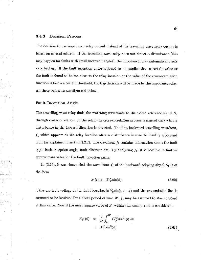
64
3.4.3 Decision Process
The decision to use impedance relay output instead of the travelling wave relay output is
based on several criteria. If the travelling wave relay does not detect a disturbance (this
may happen for faults with small inception angles), the impedance relay automatically acts
as a backup. If the fault inception angle is found to be smaller than a certain value or
the fault is found to be too close to the relay location or the value of the cross-correlation
function is below a certain threshold, the trip decision will be made by the impedance relay.
All these scenarios are discussed below.
Fault fnception Angle
The travelling wave relay finds the matching wavefronts to the stored reference signal ,92
through cross-correlation. In the relay, the cross-correlation process is started only when a
disturbance in the forward direction is detected. The first backward travelling wavefront,
/1 which appears at the relay location after a disturbance is used to identify a forward
fault (as explained in section 3.2.2). The wavefront /1 contains information about the fault
type, fault inception angle, fault direction etc. By analyzing ,fi, it is possible io find an
approximate value for the fault inception angle.
In (3.15), it was shown that ihe wave front /1 of the backward relaying signal ^9r
is of
the form
^91(t) = -2Vrsin(Q) (3.60)
if the pre-fault voltage at the fault location is Vo sin(øt + /) and the transmission line is
assumed to be lossless. For a short period of time W , i, may be assumed to stay constant
at this value. Now if the mean square value of ,91 within this time period is considered,
# I,* +vfsin2(þ) at
+Vo2 sin2(þ)
Ês, (0) ^,
(3.6 i)

65
A small value of Rs, (0) will indicate a fault with a small inception angle ó. If ó is close
to zero, the travelling wave relay is disabled and impedance relay output can be used to
trip ihe breaker.
Close-up Fault
Since the travel time of wavefronts is very short for a close-up fault, the successive refl.ections
cannot be distinguished in the relaying signals. As a result, the correlation process may
not provide a clear peak corresponding to the fault location. However, for a close-up fault,
the amplitude of the relaying signal can be high (depending on þ) and may increase rapidly
following a ramp characteristic within the first few milliseconds. The cross-correlation
function output (Þsr5, may show several peaks, but may lack any distinct peak. For a close-
up fault, a high dc level can be observed in the correlation output. The mean value Õgrg, of
the cross-correlation function can be used to identify such a situation where there are several
peaks in the output, but without any distinct peak. The output Õ5r5, is averaged over a
time period equal to the travel time f of the transmission line being protected. The average
value Õgrg, is compared with the root mean square value of the cross-correlation output
Õ.sr,grr,,"". The ratio À between Osrs, and Qsrsrr^, could be used to identify situations
when the correlation output does not have a clear peak.
À : =õ"'"'Q srsrr*,
fi J| Õs,s'dt(3.62)
For a fault very close to the measuring location, À shows a value close to unity. However,
the indication given by À is not always reliable and could show lower values for some close-up
faults.
On the other hand, the cross-correlation output of the travelling wave relay will show
a short fault distance for a close-up fault (the maximum peak among the several peaks
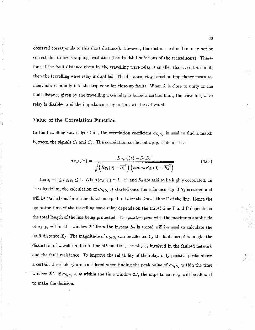
66
observed corresponds to this short distance). However, this distance estimation may not be
correct due to low sampling resolution (bandwidih limitations of the transducers). There-
fore, if the fault distance given by the travelling wave relay is smaller than a certain limit,
then the travelling wave relay is disabled. The distance relay based on impedance measure-
ment moves rapidly into the trip zone for close-up faults. When À is close to unity or the
fault distance given by the travelling wave relay is below a certain limit, the travelling wave
relay is disabled and the impedance relay output will be activated.
Value of the Correlation F\rnction
In the travelling wave algorithm, the correlation coefficient ogrg, is used to find a match
between the signals ,5r and ,52. The correlation coefficient øgrs, is defined as
osrsz(r): (3.63)
Here,-1 1oSrS, (1. Whenlosrsrl =l,Srand,S2aresaidtobehightycorrelated. In
the algorithm, the calculation of osrg, is started once the reference signal ,92 is stored and
will be carried out for a time duration equal to twice the travel time f of the line. Hence the
operating time of the travelling wave relay depends on the travel time f and t depends on
the total length of the line being protected. The posi,ti,ue pealc with the maximum amplitude
of osrs, within the window 2f from the instant ,92 is stored will be used to calculate the
fault distance X¡. The magnitude of os.sz can be affected by the fault inception angle, the
distortion of waveform due to line attenuation, the phases involved in the faulted network
and the fault resistance. To improve the reliability of the rela¡ only positive peaks above
a certain threshold ry' are considered when finding the peak value of osrs, within the time
window 21. If o.srsz ( r/ within the time window 21, the impedance relay will be allowed
to make the decision-
,Rs,sr(r) -fi.62)
(us*aa", (o) - fr')
67
3.4.4 Design Considerations
Combining the Algorithms
The derivation of the travelling wave information from the measured voltage and current
signals and the calculation of impedance -are carried out simultaneously. The travelling
wave relay and the impedance relay use the same voltage and current signals, but what is
useful for one relay becomes the noise for the other. The travelling wave relay depends on
the high frequency transient signals, and hence the 60Hz main frequency component has to
be removed from the measured waveforms. On the other hand, the impedance relay uses
the fundamental frequency component and the high frequency noise has to be filtered out.
The travelling wave signals contain high frequency transients and hence the voltage
and current signals need to be sampled at a high sampling rate. A travelling wave fault
detection scheme must consider transient generated frequencies as high as SkHz [58]. Hence
the voltage and current signals will have to be sampled with a sampling rate of at least
10kHz according to the Nyqui,st theory [62]. The frequencies present in the transient signals
might vary depending on the fault location and other line conditions [4, 58].
Since only the fundamental power frequency component is of interest for a distance
relay based on impedance measurement, the impedance relay does not need such a high
sampling rate. When the two algorithms are cascaded, the sampled values used for the
travelling wave algorithm may contain frequency components that will become noise to
the impedance algorithm. In order to avoid sampling the same signals at two different
frequencies, the samples of voltage and current obtained for the travelling wave relay a,re
decimated to achieve a lower sampling rate for the impedance relay. To avoid aliasing,
the sampied signals have to be filtered using an anti-aliasing filter with a suitable cut-off
frequency before decimation [63]. A one cycle DFT is capable of calculating the fundamental
components, while rejecting any harmonics of the power frequency.

68
Block Diagram
A block diagram of the cascaded algorithm is shown in Fi9.3.7. The calculations of the two
algorithms are carried out in parallel. The voltage and current signals are sampled at a
rate required for extracting transient information from the waveforms. The same voltage
and current samples are supplied to both travelling wave relay and impedance relay. The
travelling wave algorithm is executed on each sample of the input signal. The input samples
to the impedance algorithm are decimated by a decimation factor ltr¿. The impedance of
the line is calculated only once in every N¿ samples. This saves the processor time which
can be used for the fast travelling wave algorithm.
In the impedance algorithm, the samples are filtered and decimated before extracting
the fundamental frequency components using the DFT. The extracted 60Hz signals are
used for the impedance calculation. The ground and phase relays calculate the phase to
ground impedance and phase to phase impedance respectively. They also check whether
the calculated impedance falls within the zone of protection set by the mho characteristics.
In the case when the impedance falls within the protection zone, a trip signal is issued.
In ihe travelling wave algorithm, the delta filter removes the fundamental component
from the measured waveforms to derive the incremental components of the voltage and
current signals. The Clarke transformation is used to obtain the modal quantities. The
modal components of the aerial mode 2 are used to derive the travelling wave signals. The
fautt d,etector checks for possible disturbances in the forward direction. A disturbance is
detected when the values of the relaying signals .91 or ^92
goes above a certain threshold. The
direction of the fault is determined by the sequence in which ,S1 and 52 exceed the threshold
value. In the case when ii identifies a forwa¡d fault, both correlator and waueþont analyzer
are activated. The wavefront analyzer checks the conditions on (3.61) and (3.62). This
block determines whether the fault inception angle is small or the fault is close to the relay
Iocation.
The correlator stores a reference signal of the forward travelling wavefront ,52 and a
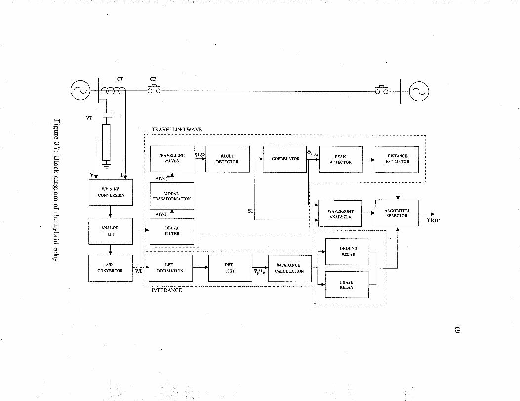
40cl-lo
ìtEÚ
ôtiÈçÞ
ûcHpHp
É!
+o
H
Ê.Eo.9
t-
I
TRAVELLING 1VAVE
\N &WCONVERSION
TRAVELLINGWAVES
IMPEDANCE
T{AVEFRONTANALYZER
II}fPEDANCE
CALCULATTON
DISTANCEESTINIATOR
(o

70
timer is activated (say ai time úi). Then it finds the cross-correlation between the stored
reference ,92 and the reflections of the wavefronts ,S1 from the fault. The correlator passes
the correlation coefficient pstsz to the pealc detector. The peak detector finds the maximum
positive peak within a time period set according to the travel time of the line and register
the time (say ú2) at which the maximum peak is detecied if the peak is above the threshold
t/. The d,istance est'i,rnator uses the times ú1 and t2 as inputs and estimates the distance to
the fault. If ihe distance is within the protection zone, a trip signal is issued.
For the protection zone of the travelling wave relay, there is a lower limit and a higher
limit. The lower limit is set to avoid discrepancies arising from distance calculations of close-
up faults and the higher limit is set to avoid faults on the adjacent line being recognized as
internal faults. The wavefront analyzer investigates the iniiial wavefront 5r and estimates
whether the fault originated with a small inception angle or the fault is too close to the
relay location for the travelling r¡/ave relay to give an accurate result. Depending on the
decision of the wavefront analyzer, the algori,thm selector determines which algorithm can
be confidently used to issue the trip signal. Even if the wavefront analyzer decides to use
the travelling v/ave relay, in the case where the fauit distance falls below the lower limit,
the trip decision is left to the impedance relay.
3.5 Operating Principle of the Hybrid Algorithm
The distance protection scheme based on impedance measurement moves rapidly into the
trip zone for close up faults. The need for speeding up is towards the reach point of the
relay. The travelling wave relay is capable of quickly detecting faults close to the reach
point of the impedance relay as well as faults beyond the reach point depending on the
maximum distance setting of the travelling wave based algorithm. The maximum setting
of the distance which can be accurately calculated depends mainly on the accuracy of the
measuring transducers. The remaining fraction of the line beyond this setting can only
be covered in a zone 1 iime by some kind of inter-trip scheme. Hence the travelling wave

77
information will be effectively used to identify faults towards the reach point of the line while
impedance mea^surement will be utilized to handle the faults close to the relay location. The
output of the two algorithms can be combined in different configurations to satisfy various
protection requirements while improving the reliability and speed of the overall scheme.
In this thesis, we look at two methods (or two algorithms) of combining the travelling
wave information with the impedance measurement to achieve reliability and speed in the
proposed cascaded protection scheme.
3.5.1 Algorithm One
The first algorithm investigates how the speed of the primary protection can be improved
while maintaining a high reliability level. Here, the trip decision is always made by the
travelling wave relay except under the following conditions:
¡ the fault detector completely fails to identify a disturbance on the line. This could
happen when the fault inception angle is zero and the fault is away from the relay
location.
the wavef¡ont analyzer decides that the initial wavefronts do not caïïy enough infor-
mation to detect a fault condition. This could happen when the fault inception angle
is near zero.
the wavefront analyzer may decide that a fault is too close to the relay location for
the travelling wave measurement.
the fault distance calculated by the travelling wave relay is smaller than the lower
limit (the upper limit is higher than the reach of the impedance relay)
the cross-correlation output doesn't show a clear peak above the set threshold and is
hence unable to estimate the distance to the fault.

72
Under any of the above circumstances, the impedance relay acts as a backup io the
travelling wave relay. A flowchart explaining the first aigorithm is shown in Fig.3.8. The
impedance is calculated after every Nff sample. The figure is self-explanatory. If for any
reason the travelling wave relay does not detect the fault condition, the impedance relay
acts as a backup.
Figure 3.8: Flowchart for algorithm 1
Fault is on theprotected line?
'l'WR -'fc¡vcling rvavú NIÂy
IRZL -'¿tt¡c I of irnpetlucc rclay

tò
3.5.2 Algorithm Two
The second algorithm investigates methods of improving the relay reach and reliability of
the combined algorithm. Here, the trip decision is always "tri,ggered" by the zone2 element
of the impedance relay. The main objectives of the second algorithm are:
¡ to improve the reliability of the combined protection scheme;
o to increase the relay reach;
o to accelerate the zone 2 protection of the impedance measurement technique;
o to increase the reliability by reducing the dependency on an end-to-end communication
channel.
The measured impedance enters the zone 2 of the impedance characteristic before reach-
ing the zone L. Therefore, for faults that occur in zone 1, the combination of zone 2 element
and travelling wave information could provide faster operating times than that provided with
the zone 1 of the impedance relay alone. The zone 2 eiement prevents possible mal-operation
of the travelling wave relay from non-fault transients caused by switching operations. Since
the zone 2 element triggers the cascaded algorithm, the reliability of the protection scheme
is very high, but the fault detection time will be shorter than the primary protection of the
impedance relay.
The faults that occur at the far end of the line have long travel times. The transient
waves generated by such faults will have a low bandwidth. The bandwidth requirement
of measu¡ing transducers are low for such faults. When a fault occurs towards the end
of the line, the iravelling wave relay can calculate the distance to the fault accurately.
Therefore, the relay reach of the combined scheme can be extended almost to the far end
of the line. The resolution of the distance meåsurement will depend on the sampling rate
of the waveforms. Wiih the high sampling rates used in the travelling wave algorithm, it is

74
possible to extend the relay reach to about 90%-95% in long EHV lines depending on the
accuracy of the measuring transducers used.
The standard practice in distance protection is io set the primary reach to about 80%
of the line length. A fault on the remaining 20% of the line will fall into zone 2 of the
protection scheme. The zone 2 element in a distance relay involves an added delay to allow
a primary element in the adjacent line to operate first for a fault on the adjacent line which
falls within the zone 2 reach. However, this delay can be too long to maintain the stability
of a highly loaded system. A direciional protection scheme with two relays at the opposite
ends of the line connected through an end-to-end communication protocol will be a solution
to improve the fault isolation time. A transfer-trip or permissive signal is used to command
the relay at the remote end of the transmission line to trip the breakers open. The transfer-
trip signal travels via the communication network and when received by the remote end
relay a breaker irip signal is issued.
However, the reliability of teleprotection schemes will depend on the reliability of the
communication channel. Besides, the communication equipment can be very expensive. As
an alternative solution, the output of the travelling wave relay is utilized to accelerate the
zone2 element of the impedance relay in the hybrid algorithm. \Mhen the calculated distance
of ihe travelling wave relay shows a fault on the protected line and the measured impedance
enters zone 2 of the impedance characteristic, the zone 2 element is accelerated. This
method not only eliminates the necessity of the costly communication channel, but is also
capable of achieving faster tripping times compared to a teleprotection scheme. An analog
teleprotection scheme using frequency-shifting techniques to transmit the transfer-trip signal
can have back-to-back latencies greater than 10 milliseconds. Adding the operating time of
the remote relay and the propagation delay of the communication channel to this latency
results in higher values for the fault detection time than the combined algorithm.
The Fig.3.9 shows a fl.ow chart of the protection algorithm. Zone 2 acts as the "starter"
element for the travelling wave technique. If the travelling wave relay is unable to detect

75
a fault (in the rare event of a line to ground fault that occurs when the line voltage at the
fault location is zero), the zone 1 or the zone2 element of the impedance relay will detect
the fault depending on the fault location. If the travelling wave relay fails to detect the
fault in the second zone, the zone2 element will have the standard (eg. 30 cycle) delay. The
hybrid algorithm operates faster than the zone 1 or zone 2 element of the impedance relay
alone. The travelling wave relay enables a "fast zone 2 element" and allows the impedance
relay to detect faults quickly on almost the fult length of the line. The overall result is a
secure and fast protection scheme.
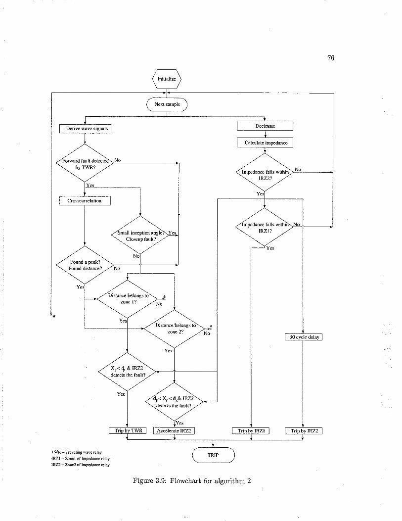
76
Calculate irnpedance
Found a peak?
Found distance?
Distance belongs tozone I ?
Distance belongs tozone2?
xf<dP &.tRZzdetects the fault?
\ < d"& rRz2
T\,VR - Tmveling wave relay
lRZl -Znnel of impedance relay
lRZZ -'Znne2 of im¡ædance relay
Figure 3.9: Flowchart for algorithm 2

Chapter 4
Simulation Studies
4.1 lntroduction
The ideal approach to study the transient phenomena in a power system is to capture
and record the transients using wide bandwidth transducers and recording equipment and
then analyze these waveforms. However, capturing transient signals this way representing
all possible scenarios is not realistic. An alternative technique is to simulate the power
system using a suitable electromagnetic transient program (EMTP). The EMTP programs
available in the market today represent the power system components wiih realistic models.
These models usually match the main characteristics of the components while keeping the
complexity of the models to a minimum. The power system simulation programs not only
present a convenient way to generate the signals required to analyze a certain feature (eg.
the protection scheme in this case), but also allow the user to study the worst case scenarios
that are unlikely to be generated in the real world.
In order to verify the concept of the hybrid relay discussed in the previous chapter, sim-
ulation studies were carried out on a three phase power system using an EMTP program. A
power network can have many possible system configurations. The main objective here was
to select a more practical system configuration to identify the feasibility of the proposed
protection scheme. Rather than testing the protection scheme on many different configura-
77

78
tions, it was decided to choose a single configuration based on a real system and prove the
concept with different fault situations. Since the main application of the hybrid protection
scheme is in EHV long transmission systems, a model based on 500 kV system from Man-
itoba to Minnesota was used for simulation studies. The 500 kV system was modelled as
a simple power system represented by a single circuit, three phase transmission line with
lumped parameter equivalent sources at each line end. The simulations were carried out
using PSCAD/EIVITOç rÀ1 [12] software. This chapter presents the details of the power
system configuration chosen, the simulation studies carried out and the simulation results.
4.2 SystemConfiguration
The three phase power network chosen for simulation studies is based on Manitoba Hydro's
Dorsey-Forbes-Chisago network which spans from Southern Manitoba to Minnesota. A
detailed diagram of the power network with its main electrical components is shown in
Fig.4.1. The two major 500 kV transmission lines connect the Dorsey and Forbes, and
Forbes and Chisago substations respectively. The Dorsey-Forbes line is 537 km long and the
Forbes-Chisago line is224 km long. The Chisago substation is connected to King/Kohlman
with a 345 kV double transmission line. The Dorsey-Forbes-Chisago EHV long transmission
network gives a model of a real system for testing the performance of the proposed hybrid
scheme.
For simulation purposes, only the 500 kV transmission system was considered. For sim-
plicit¡ the series compensation on the two lines were removed. The 345 kV system was
replaced with its lumped parameter equivalent source at the Chisago busbar. When evalu-
ating the surge propagation along a transmission line, the significantly shorter delay within
the windings of a transformer and generator enable these elements to be considered as
lumped pa.rameter approximations [6]. Hence the power system was represented by a single
circuit, three phase transmission line with its lumped parameter equivalent sources at each
end. The generators were modelled in their three phase equivalent circuit in which the posi-

79
ChlsaSo
Figure 4.1: Network diagram for 500
L¡nc le¡Blhs:Dorecy-Forb*:537kmFortrcs-Chisago:224kn(h¡sago - King/Kohlmm : 82krn
kV system
Figure 4.2: Line transposing intervals of the 500kV line
tive sequence lumped reactance was calculated from the fault levels (short circuit capacity).
This short circuit capacity value can be varied according to the simulation requirements.
The overhead transmission lines rffere assumed to be uniformly distributed along its length
and the line impedance values were calculated, for all frequencies chosen, from the line
physical construction by taking into account the effects of line spacing, conductor geome-
tr¡ conductor internal impedance, and earth return path. The line was considered fully
transposed since the physical line transpositions in the 500 kV line were incorporated in
the simulation model. The line transposing positions are shown in Fig.4.2.
The simplified circuit equivalent used for simulations is shown in Fig.4.3. The trans-
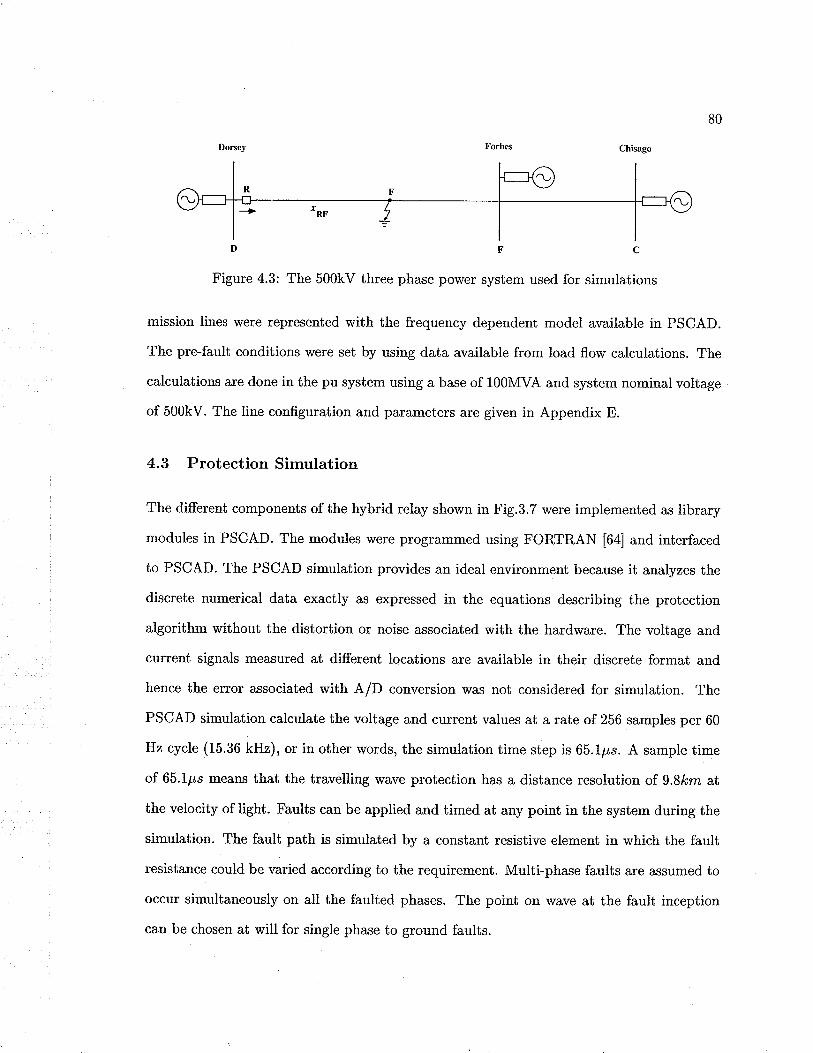
80
FC
Figure 4.3: The 500kV three phase power system used for simulations
mission lines were represented with the frequency dependent model available in PSCAD.
The pre-fault conditions were set by using data available from load flow calculations. The
calculations are done in the pu system using a base of 100MVA and system nominal voltage
of 500kV. The line configuration and parameters are given in Appendix E.
4.3 ProtectionSimulation
The different components of the hybrid relay shown in Fig.3.7 were implemented as library
modules in PSCAD. The modules were programmed using FORTRAN [6a] and interfaced
to PSCAD. The PSCAD simulation provides an ideal environment because it analyzes the
discrete numerical data exactly as expressed in the equations describing the protection
algorithm without the distortion or noise associated with the hardware. The voltage and
current signals measured at different locations are available in their discrete format and
hence the error associated with A/D conversion was not considered for simulation. The
PSCAD simulation calculate the voltage and current values at a rate of 256 samples per 60
Hz cycle (15.36 kHz), or in other words, the simulation time step is 65.lps. A sample time
of 65.1¡.rs means that the travelling wave protection has a distance resolution of.9.8lcm at
the velocity of light. Faults can be applied and timed at any point in the system during the
simulation. The fault path is simulated by a constant resistive element in which the fault
resistance could be varied according to the requirement. Multi-phase faults are assumed to
occur simultaneously on all the faulted phases. The point on wave at the fault inception
can be chosen ai will for single phase to ground faults.

B1
PSCAD generâ,tes instantaneous voltage and current signals at different locations. The
voltage and current measurements taken at the relay location are used in the protection
algorithm. The calculations of both travelling wave and impedance algorithms are carried
out in parallel. The signals sampled at 15.36kH2 are low pass filtered and re-sampied at
480H2 before using them for the impedance calculations. A third order Butterworth filter
was used for filtering. The down-sampling provides 8 samples per a 60Hz cycle for the
impedance estimation. The procedures involved in the simulation of the travelling wave
and impedance algorithms are described separately below.
4.3.L Tlavelling'Wave Algorithm
The program calculates the instantaneous values of the incremental components of the
voltage and current waveforms. The incremental signals are generated by subtracting the
measured signals taken exactly one cycle before from the present samples. The incremental
voltage and current phase signals are decoupled into three independent modes (mode 1,
mode 2 and mode 3) using the Clarke transformation matrices given by (3.29) and (3.30).
Since the three phase system is fully transposed and has balanced line terminations, the
effects of frequency dependence of the modal decomposition matrices is ignored. Mode 1
is the earth mode and mode 2 and mode 3 are aerial modes. The earth mode is frequency
dependent, highly attenuated and has a slower velocity compared with the aerial modes.
The distance obtained using earth mode was found to be inaccurate. The aerial modes are
not much affected by the varying ground resistivity over a wide frequency band and give
sufficiently accurate results [59]. In our implementation, the relaying signals of mode 2 are
used for the travelling wave algorithm. Mode 2 has a propagation velocity of 295lrmf ms
and a modal surge impedance of.276Q.
Fig.4.4 shows the three phase voltage and current waveforms, the incremental phase
components, and the incremental modal quantities for a three phase to ground fault at a
distance32Skmawayfromtherelaylocation (*nr:325km) online DFinFig.4.3. The

82
incremental components clearly show the presence of travelling wavefronts in the voltage
and current signals.
The incremental components of the aerial mode 2 are used to derive the relaying signals
,S1 and .92.
.9Í')
st')
Ar(2) + 2Q).6¿(z)
6rQ) - gQ).6¿Q)
(4.1)
(4.2)
where Z[') i" the surge impedance of mode 2.
time(ms)
Figure 4.4: The fault transients generated by a three phase to ground fault: r¿p :325km
The fault detector checks for possible disturbances on the transmission line by checking
the sequence in which the relaying signals ,Sr and Sz Eo above a predetermined threshotd.
Voltage Current
Increuiental Voltage
o MloM2 vM3

83
When the fault detector identifies a disturbance in the forward direction, it issues a forward
trigger signal thai triggers the correlator. The correlator stores a section of the forward
relaying signal Sz. A storage window of 10 samples, (ltr: 10), or in other words a sample
window of duration tw : 0.65Lms r,vas found to be optimal for detecting most of ihe fauli
conditions.
The storage window includes some samples before and some samples after the fault
disturbance to ensure the best representation of the wavefront. The literature [36] and the
simulations showed thai a storage window containing 3 samples before (rt : B), and Z
samples after the disturbance (ro :7) was capable of producing clear peaks in the cross-
correlation output. The correlator finishes storing a section of the relaying signal .92 at time
zr. The correlator finds the cross-correlation between the stored signal ^92 and sections of
backward relaying signal 51.
The sections of the relaying signals ,9r and .92 have different mean levels on which
the required travelling wave components are superimposed. To find a useful correlation,
the mean values of the signals ,5r and ,52 are removed before finding the cross-correlation.
The cross-correlation function is then normalized to find the correlation coefficient. The
correlation output is calculated for a time period equal to twice the travel time of the line
being protected, 2f from the instance the correlator finishes storing the signal 52.
Fig.4.5 shows the relaying signals, the forward trigger signal and the correlator output
for the above fault. The forward trigger signal is kept high for a time period equal to 2f
plus the storage time of the signal 52, ie a total duration of [2[ 1- (n"lN)t.]. For the line
DF,2l :3.64ms.
The peak detector finds the positive peaks of the correlator output above a certain
threshold. The threshold was set to 0.25 p.u. to eliminate false peak identification due to
the effect of noise. The maximum positive peak of the correlator output within the time
period 2l is used by the distance estimator to calculate the distance to the fault. The
time at which the correlator output becomes maximum, T2 corresponds to the distance to

84
Voltage
tr Vâ oVo VV"
Cunent
40
20
io-20-40
4
2
{oè
4
3
tirne(ms)
Figure 4.5: The relaying signal for a three phase fault: z¿p :325lcm
the fault. For the three phase fault described above, n : L.63ms, T2 : 3.84ms, and the
calculated distance to the fault r¿p :325.981cm.
4.3.2 Impedance Measurement Algorithm
The apparent impedance seen at the relay location is calculated using the voltage and. cur-
rent signals. In our simulations, we use 8 samples of voltage and current signals per 60Hz
cycle for impedance estimation. That means, the samples used for travelling v/ave algorithm
are decimated by a factor of 32. Instead of using a DFT (as shown in Fig.3.7), the FFT
block component available in the PSCAD program was used to extract the fundamental
60Hz components of voltage and current signals. Separate FFT blocks were used to find
the 60Hz voltage, 60Hz current and symmetrical components. The fundamental compo-
Relaying Signals
Forward Trigger Signal and Correlator Output
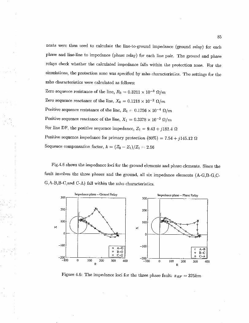
B5
nents were then used to calculate the line-to-ground impedance (ground relay) for each
phase and line-line to impedance (phase relay) for each line pair. The ground and phase
relays check whether the calculated impedance falls within the protection zone. For the
simulations, the protection zone was specified by mho characteristics. The settings for the
mho characterisiics were calculated as follows:
Zero sequence resistance of the line, á : 0.8211 x I0-3 ef m
Zero sequence reactance of the line, X6 : 0.1218 x t0-2 ef m
Positive sequence resistance of the line, R1 : 0.1256 x t0-4 e/rn
Positive sequence reactance of the line, X1 : 0.BJZ8 x l0-3 e/mFor line DF, the positive sequence impedance, Zt : g.4J + j1gl.4 e
Positive sequence impedance for primary protection (g0%) : 7.54 + jL41.LZ O
Sequence compensation factor, Ic : (Zo - ZùlZt :2.56
Fig.4.6 shows the impedance loci for the ground elements and phase elements. Since the
fault involves the three phases and the ground, all six impedance elements (A-G,B-G,C-
G,A-B,B-C,and C-A) fall within the mho characteristics.
Rp
Figure 4.6: The impedance loci for the three phase fault: z¿¡ : BL\lcm
Impedance plane - Cround Relay Ínpedance plane - Phase Relay

86
4.3.3 Combining the Algorithms
Fig.4.7 shows the three phase voltage and current signals and the trip signals issued by the
travelling wave and impedance algorithms sepa,rately for the three phase to ground fault
discussed above. The travelling wave relay estimates the distance to ihe fault to be 325.9
km. Since this is within the protected line length, a trip signal is issued by the travelling
wave relay 5.4ms after the fault inception. The impedance relay detects the fault 11-.7ms
after the fault inception. The wavefront analyzer analyzes the first wavefront that appeared
at the relay location to see whether a steep wavefront was created by the fault transients.
For this fault, the wavefront analyzer decides that the travelling wave algorithm can make
a reliable estimation of the fault distance. Since the fauli distance is within the reach, the
hybrid algorithm issues a trip signal without waiting for the decision of the impedance relay.
The combined algorithm speeds up the trip decision by 6.3ms in comparison to the case
when only the impedance relay was present.
4.4 Simulation Cases
The operating principle of the hybrid algorithm was explained in the above section using
a three phase to ground fault example. However, the most frequent disturbances present
in transmission networks are the single line io ground faults. The operating principle of
the hybrid relay is similar for single.phase-to-ground faults, but special cases can be found
when the fauli inception angle becomes very small. In order to show the operating strategy
of the hybrid rela¡ several examples are considered here. The reach of the impedance relay
is set to 80% of the line length while the travelling wave algorithm accepts disturbances
between lSVo and 95% of the line.
Fig.4.8 shorvs the waveforms related to a phase B to ground fault at rRF :270km. The
fault inception angle, d : 600. The fault detector identifies a forward disturbance at 0.92ms
after the fault inception. The correlator shows a peak at 3.39ms which corresponds to a
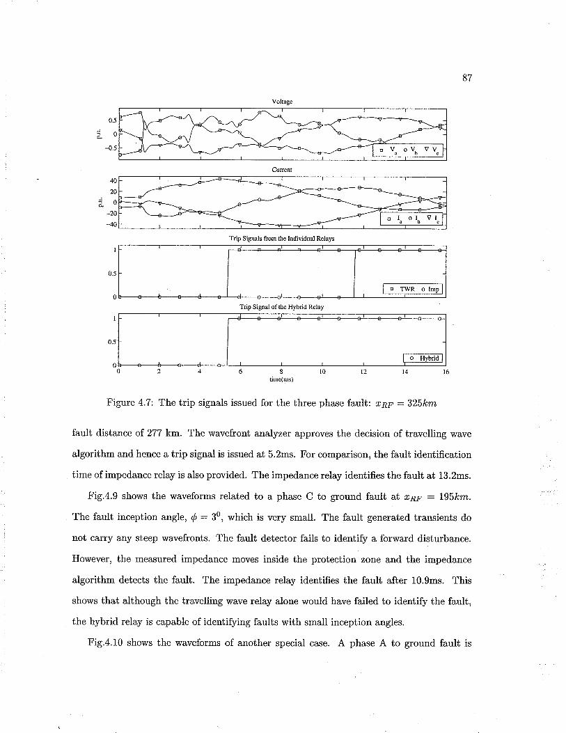
87
0.5
¿^o
-0.5
40
20
-.i oo_20
-40
I
0.5
0
I
0.5
08
tirne(ms)
Figure 4.7: The trip signals issued for the three phase fault: r¿p :325lcrn
fault distance of 277 km. The wavefront analyzer approves the decision of travelling wave
algorithm and hence a trip signal is issued at 5.2ms. For comparison, the fault identification
time of impedance relay is also provided. The impedance relay identifies the fault at 13.2ms.
Fig.4.9 shows the waveforms related to a phase C to ground fauli at rpp : 1,95km.
The fault inception angle, d : 30, which is very small. The fault generated transients do
not carry any steep wavefronts. The fault detector fails to identify a forward disturbance.
However, the measured impedance moves inside the protection zone and the impedance
algorithm detects the fault. The impedance relay identifies the fault after L0.9ms. This
shows that although the travelling wave relay alone would have failed to identify the fault,
the hybrid relay is capable of identifying faults with small inception angles.
Fig.4.10 shows the waveforms of another special case. A phase A to ground fault is
Voltage
Cunenl
Tri¡r Signals frorn the Individua.l Relays
Trip Signal of the Hybrid Relay
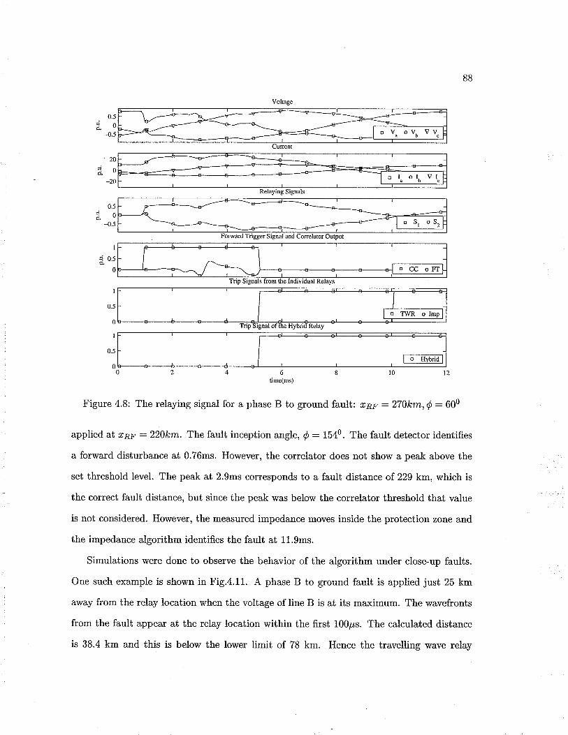
BB
0.5jno-
-.0.5
20
io-20
0.5
io-{.5
I
i 0.5a0
I
0.5
0
I
0.5
0t " Hyb.'d I
6tirne(ms)
Figure 4.8: The relaying signal for a phase B to ground fault: rRF :270km,d : 600
applied at rpp :2201cm. The fault inception angle, ó: 1540 - The fault detector identifies
a forward disturbance at 0.76ms. However, the correlator does not show a peak above the
set threshold level. The peak at 2.9ms corresponds to a fault distance o1229 km, which is
the correct fault distance, but since the peak was below the correlator tb¡eshold that value
is not considered. However, the measured impedance moves inside the protection zone and
the impedance algorithm identifies the fault at 11.9ms.
Simulations were done to observe the behavior of the algorithm under close-up faults.
One such example is shown in Fig.4.11. A phase B to ground fauli is applied just 25 km
away from the relay location when the voltage of line B is at its maximum. The wavefronts
from the fault appear at the relay location within the first 100ps. The calculated distance
is 38.4 km and this is below the lower limit of 78 km. Hence the travelling wave relay
Volmge
Cunent
Relaying Signals
from the Individual Relays
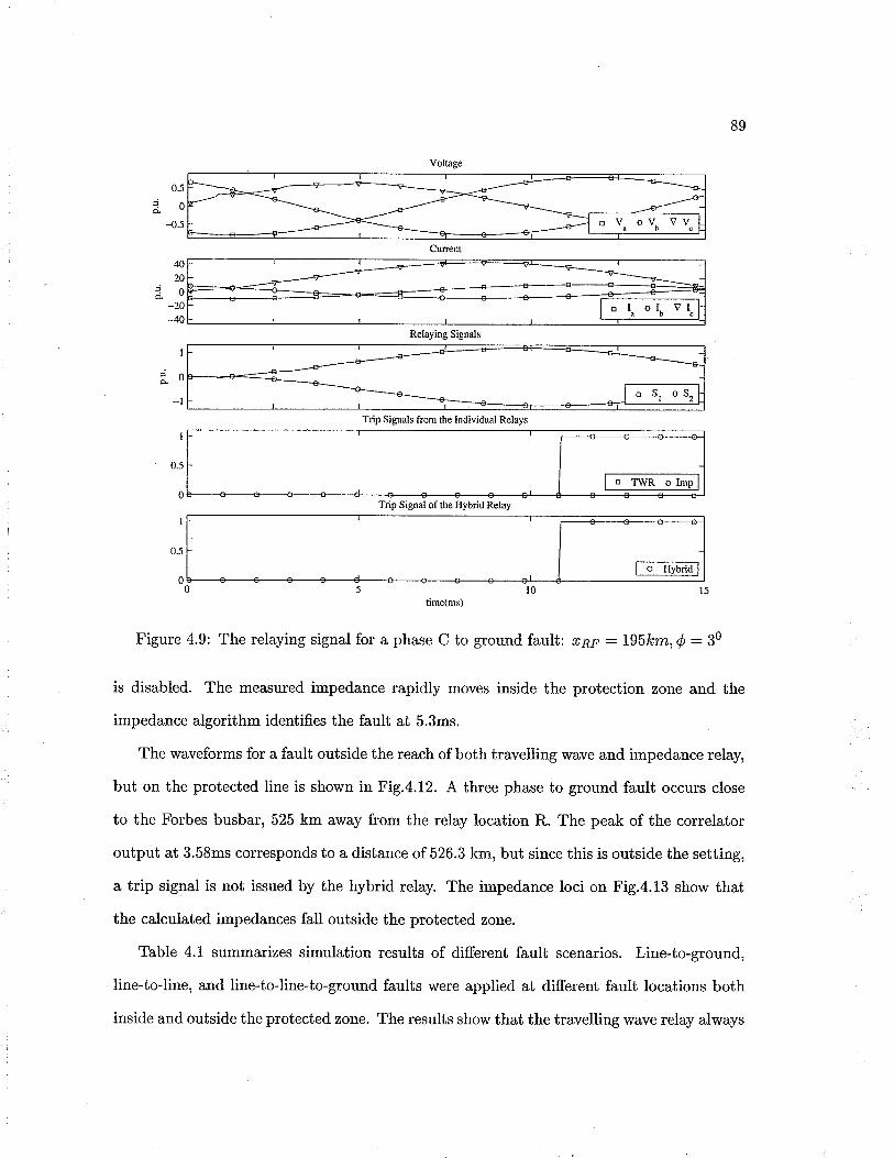
89
0.5
:.0-0.5
I
0.5
0
I
0.5
0
tilne(nìs)
Figure 4.9: The relaying signal for a phase C to ground fault:
40
20
É0-20_40
I
ioè--l
t" TwR "
Irnpl
Trip Signal of the Hybrid Relay
l- " Hyì'td I
t0 l5
rrRF : L\\lem,Ó:30
is disabled. The measured impedance rapidly moves inside the protection zone and the
impedance algorithm identifi.es the fault at 5.3ms.
The waveforms for a fault outside the reach of both travelling wave and impedance relay
but on the protected line is shown in Fig.4.12. A three phase to ground fault occurs close
to the Forbes busbar, 525 km away from the relay location R. The peak of the correlator
output at 3.58ms corresponds to a distance of 526.3 km, but since this is outside the setting,
a trip signal is not issued by the hybrid relay. The impedance loci on Fig.4.13 show that
the calculated impedances fall outside the protected zone.
Table 4.1 summarizes simulation results of different fault scenarios. Line-to-ground,
line-to-line, and line-to-line-to-ground faults were applied at different fault locations both
inside and outside the protected zone. The results show that the travelling wave relay always
Voltage
Cunent
o Vo oVn VV"
Relaying Signals
Trip Signals from the Individual Relays

90
0.5
:.0-{.5
40
20
åo_20
40
2
3o
0.2
.04o -{.2
-0.4OCC
Trip Signals from the Individual Relays
trTWRo
tirne(ms)
Figure 4.10: The relaying signal for a phase A to ground fault: rRF :2201cm,ó:1540
detects the faults quickly when steep wavefronts are present. The impedance relay is slow
compared to the travelling wave algorithm, but detects faults under all possible scenarios
within its reach. The overall performance of the hybrid relay is superior to either travelling
wave or impedance relay alone.
4.5 Accelerating Zone 2 Protection
In section 3.5.2, we discussed how the hybrid relay arrangement could be used to accelerate
the zone 2 protection of a distance relay. The hybrid relay is a single-ended scheme, or in
other words, the relay uses the information from only one end of the line. The idea of using
a single-end information is to get rid of the expensive communication channel. In order
to study the behavior of the hybrid relay scheme in the proposed algorithm, simulations
I
0.5
0t2
Voltage
Curent
Relaying Signals
Correlator Output
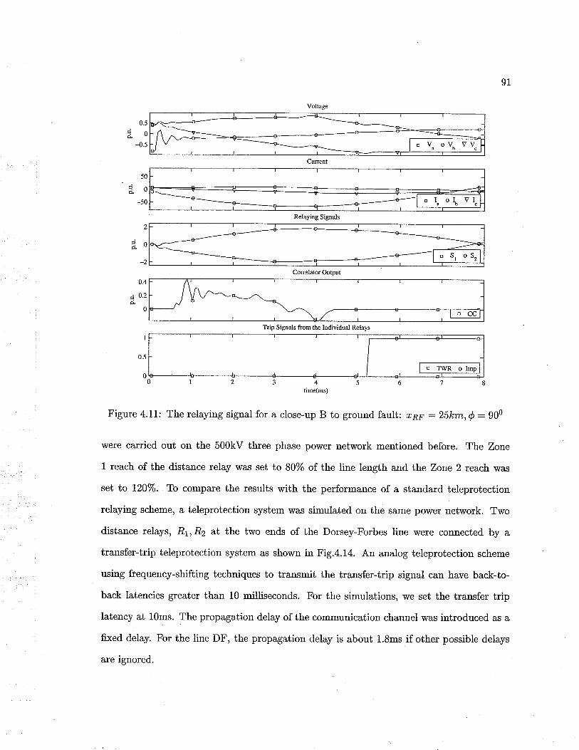
91
50
åo-50
2
jno-
0.4
102a0
I
0.5
ooTWRo
0
Figure 4.11: The relaying signal for a close-up B to ground fauit: z¿p :25km,d : g00
were carried out on the 500kV three phase power network mentioned before. The Zone
1 reach of the distance relay was set to 80% of the line length and the Zone 2 reach was
set to 120%. To compare the results with the performance of a standard teleprotection
relaying scheme, a teleprotection system was simulated on the same por¡/er network. Two
distance relays, Rt, Rz at the two ends of the Dorsey-Forbes line were connected by a
transfer-trip teleprotection system as shown in Fig.4.14. An analog teleprotection scheme
using frequency-shifting techniques to transmit the transfer-trip signal can have back-to-
back latencies greater than 10 milliseconds. For the simulations, we set the transfer trip
latency at L0ms. The propagation delay of the communication channel was introduced as a
fixed delay. For the line DF, the propagation delay is about L.8ms if other possible delays
are ignored.
345tirne(ms)
Voltage
Current
Relaying Signals
Correlator Output
Trip Signals from the Individual Relays

ot
Voltage
Cunent
Relaying Signals
Corelator Output
Figure 4.L2: The relaying signal for three phase to ground fault: ø¿¡ :525lcm
?JO
200
x t.50
100
50
0
-50
-r00-r00
Figure 4.13: The impedance loci for three phase to ground fault: øRr :525km
Inrpedance plane - Ground Relay Impedance plane - Phrse Relay400
350
3m
250
200
r50

93
Fault rÍ óo tp tt- tz t7 ItuA-G
B-G
C-G
AB-G
A-G
AC
ABC-G
B-G
C-G
AC-G
ABC-G
325
270
195
425
220
490
325
25
245
95
525
90
60
4
154
270
45
3.84
3.39
4.9
2.st
5.5
3.84
3.0
1.6
5.et
5.4
5.2
5.8
5.96
5.4
5.1
4.7
14.5
10.3
10.9
13.5
11.9
TT.7
5.3
9.3
7.2
5.4
5.2
10.9
5.8
1i.9
5.96
5.4
5.3
5.1
4.7
325.4
277.2
42t
22el
488
325.4
239.2
95.7
526.31
r I : The distance to the fault
ó : The fault inception angle
tp : The time at which the peak of correlator output occurs
tt- : The fault detection time of the travelling wave relaytz : The fault detection time of the impedance relayt,¡ : The time at which the hybrid relay issues the trip signalrtw : The distance calculated by the travelling wave relay
I The correlator pealc i,s below threshold,
tThe calculated distance outs,í.de the reach
Let us consider a three phase to ground fault to demonstrate the operating principle of
the algorithm. The fault occurs at a location 500 km away from D towards F, The voltage
and current signals seen by the relays ,R1, and R2 arcshown in Fig.4.15.
The loci of the impedance seen by the two relays -Rr and R2 arc shown in 4.16. The
impedance calculation of the relay -R1 falls inside zone 2 while the impedance loci of the
relay at the other end enters inside zone I.
Fig.4.17 shows the relaying signals of the travelling wave relay, the correlator output,
and the various trip signals issued by relays at both ends of the line. The fault detector
detects a forward fault 1.7ms after the fault occurred. The correlator output shows a peak

94
Forbæ
)Al-
Doßcy
(-
IA
Chisago
--->Rl
-->RJ
537 km 224kn
Figure 4.1,4: The 500kV line with two relays connected by a communication channel
30
20
t0
e0_t0
_20
-30
02468100246810
Figure 4.15: The fauit transients generated by three phase to ground fault: r¿p :500lcm
0.8
0.6
0.4
0.2
io4.2
-0.4
-0.6
-o.8
Voltage at Relay Rl Voltåte ût Relay R2
Curent at Relay Rl Curent at Relay R2
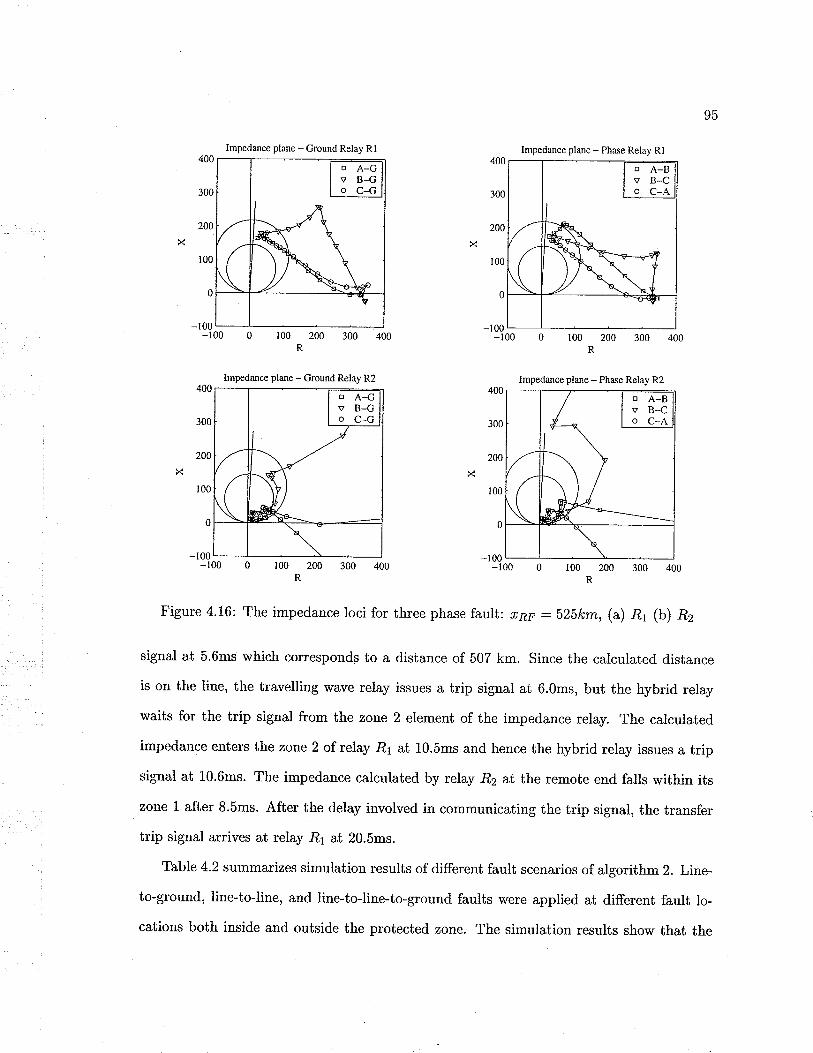
95
Inpedance plane - Ground Relay Rl lnrpedance plane - Phase Relay Rl
- 100-1 00
Iurpedarce plane - Ground Relay R2 hnpedance plane - Phase Relay R2
100 200R
Figure 4.16: The impedance loci for three phase fault: ø¿p : S25km, (u) A, (b) Ëz
signal at 5.6ms which corresponds to a distance of 507 km. Since the calculated distance
is on the line, the travelling wave relay issues a trip signal at 6.0ms, but the hybrid relay
waits for the trip signal from the zone 2 element of the impedance relay. The calculated
impedance enters the zone 2 of relay .Rr at 10.5ms and hence the hybrid relay issues a trip
signal at 10.6ms. The impedance calculated by relay ,R2 at the remote end falls within its
zone 1 after 8.5ms. After the delay involved in communicating the trip signal, the transfer
trip signal arrives at relay .R1 at 20.5ms.
Table 4.2 summarizes simulation results of different fault scenarios of algorithm 2. Line-
to-ground, line-to-line, and line-to-line-to-ground faults were applied at different fault lo.
cations both inside and outside the protected zone. The simulation results show that the

96
hybrid relay can detect faults faster than a teleprotection scheme when steep wavefronts are
present in fault transients. When a fault on the line falls in zone 2 of the impedance relay
and the travelling wave relay does not detect the fault, a 30 cycle delay is introduced to the
zone 2 trip signal. By using some kind of an inter-trip signal, such faults can be cleared
within a satisfactory time. The overall performance of the hybrid relay is superior to either
travelling wave or impedance relay alone.
I
Fault rl óo tp tt- tzz tzt t¡, tr ttp rtut
A-G
B-G
C-G
A-G
B-G
C-G
AC-G
ABC-G
325
500
420
470
445
95
525
500
35
270
-J
174
240
50
3.83
5.8
5.0
1.5
5.9ÉryLr. I
5.4
6.0
5.8
4.6
6.0
6.0
8.4
14.7
L0.2
10.1
13.6
9.0
L2.2
10.5
9.5
16.5
11.1
8.4
14.7
16.5
4TL
13.6
9.0
72.2
10.6
10.5
6.4
7t.2
i0.1
7.4
5.9
8.4
22.5
18.3
23.2
22.0
19.4
17.9
20.4
325.4
507.i
449.7
95.7
526.2
507.1
ïÍ : The distance to the fault
ó : The fault inception angle
tp : The time at which the peak of correlator output occurs
tn : The fault detection time of the travelling wave relay
tz2 : The fault detection time of the zone 2 of the impedance relay .R1
tzt : The fault detection time of the zone L of the impedance relay ,R1
tr : The fault detection time of the zone2 of the impedance relay R2
t¡ : The time at which the hybrid relay issues the trip signal
ttp : The time at which the transfer trip signal of R2 is received by l?r
ttw : The distance calculated by ihe travelling wave relay
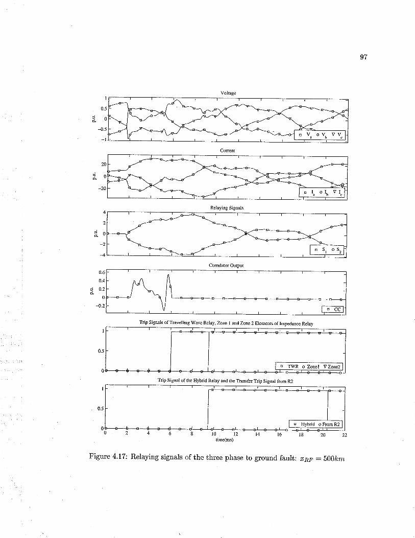
97
Voltâge
Currenl
Relaying Signals4
2
eo
4
0.6
0.4
a 0.7o
0
4.2
I
0.5
0
I
0.5
0a246ttou,n"(r*)tt14
Figure 4.17: Relaying signals of the three phase to ground
Trip Signal of the Hybrid Relay and the Trdnsfer Trip Signal from R2
16 t8
fauit: ø¿p
)^ 11
:500km
Correlator Output
Trip signals of rravelling wave Relay,Tnne L and Zone 2 Elenrents of Lnpedarce Relay
q TWR o 7.onel V Zone2
Chapter 5
Laboratory Prototype
5.1 fntroduction
A laboratory prototype of the hybrid relay algorithm was developed to test the real-time
performance of the relay. One of the main aspects of the design was to keep the cost of
the relay as low as possible. Choosing and designing hardware and software capable of
handling the extensive calculations in real time while keeping the cost low r¡/as a difficult
task. It was decided to develop the prototype with the hardware resources readily available
in the industry, identify their limitations and study the requirements for the final prod-
uct. Several configurations were attempted and numerous technical difficulties had to be
addressed before the final implementation. The simulation algorithms had to be modified
and special calculation procedures had to be chosen to decrease the processing time. In this
chapter, the hardware and software aspects of the laboratory prototype implementation are
discussed. The biggest challenge faced during the implementation was capturing voltage
and current signals ai high sampling rates required for the travelling wave relay and hence
more emphasis will be made to the details of the data acquisition system.
98
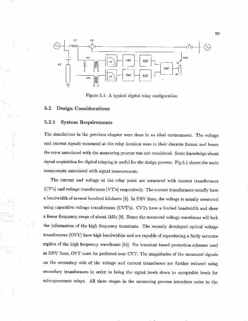
99
Figure 5.1: A typical digital relay configuration
5.2 DesignConsiderations
5.2.1 System Requirements
The simulations in the previous chapter were done in an ideal environment. The voltage
and current signals measured ai the relay location vrere in their discrete format and hence
the error associated with the measuring process was not considered. Some knowledge about
signal acquisition for digital relaying is useful for the design process. Fig.5.1 shows the main
components associated with signal measurement.
The current and voltage at the relay point are measured with current transformers
(CT's) and voltage transformers (VT's) respectively. The current transformers usually have
a bandwidth of several hundred kilohertz [8]. In EHV lines, the voltage is usually measured
using capacitive voltage transformers (CVT's). CVTs have a limited bandwidth and show
a linear frequency range of about lkHz [9]. Hence the measured voltage waveforms will lack
the information of the high frequency transients. The recently developed optical voltage
transformers (OVT) have high bandwidths and are capable of reproducing a fairly accurate
replica of the high frequency wavefronts [65]. For transient based protection schemes used
in EHV lines, OVT must be preferred over CVT. The magnitudes of the measured signals
on the secondary side of the voltage and current transducers are further reduced using
secondary transformers in order to bring the signal levels down to acceptable levels for
microprocessor relays. Ali these stages in the measuring process introduce noise to the

100
measured signal. In order to improve the signal to noise ratio, high fidelity transducers
must be used.
No signal is truly deterministic and therefore in practice has infinite bandwidth. How-
ever, the energy of higher frequency components becomes increasingly smaller so that at
a certain value it can be considered to be irrelevant. For- an impedance relay the signals
above 60Hz become noise, but a transient-based relay needs information contained in the
high frequency transients. The signals used for the travelling wave relay need not have an
upper limit for the frequency since the correlator compares the shape of the stored reference
with the reflected signals. However, analog to digital conversion will introduce an aliasing
effect due to the sampling of the continuous signals. In order to reduce the effect of aliasing,
the signals used for ihe travelling wave relay should have an upper limit in the bandwidth.
The amount of aliasing that can be tolerated is eventually dependent upon the resolution
of the system. If the system has low resolution, then the noise floor is already relatively
high and aliasing does not have a significant effect. However, with a high resolution system,
aliasing can increase the noise floor considerably. One way to prevent aliasing is to increase
the sampling rate. However, the maximum sampling rate is limited by the type of data
converter used and also by the maximum clock rate of the digital processor receiving the
data. Therefore, to reduce the effects of aliasing, analog filters must be used to limit the
input signal spectrum.
For faults on a high voltage transmission line, the transient signals can have a bandwidth
as high as SkHz [58]. It was decided that considering frequencies below SkHz is quite
adequate for travelling wave measurements. Hence signals above SkHz will have to be
filtered out in the prototype implementation. Hence the sampling rate has to be at least
L0kHz. For the implementation, it was decided to consider a sampling rate of at least three
times the Nyquist rate. In order to calculate the fundamental frequency component using
an Fast Fourier Tbansform (FFT) algorithm, the number of a samples within one 60Hz
cycle has to be a power of two. It is quite adequate to use 8 samples/cycle to calculate
101
the 60Hz signals. With a sampling rate of about 15kHz and a suitable decimation factor, B
samples/cycle can be obtained. It was found that a decimation factor of 32 and a sampling
rate of 256 samplesf cycle (15.36kH2) was suitable for our application.
The voltage and current transducer outputs are captured by the sample and hold circuit
at pre-specified time instances. These samples are then cónverted to discrete values by an
analog to digital converter (ADC). The ADC chosen must have a linear gain throughout
the input voltage range, and should not have any offset or non-linearity errors. When
nonlinearity errors are present, the values on the actual transfer function of the ADC can
deviate from a straight line. The analog input to an ADC is a continuous signal with an
infinite number of possible states, whereas the digital output is by iis nature a discrete
function with a number of different states determined by the resoiution of the ADC. Hence
some information can be lost and distortions may be introduced into the signal. This is
known as quantization noise. A high resolution ADC minimizes the effect of quantization
noise. However, the cost of the ADC increases with the increase in resolution. Analysis
of the waveforms showed that an ADC having a 12-16bit resolution can provide adequate
resolution while keeping the cost down.
The travelling wave algorithm needs to analyze information as high as 5kHz. Hence
an ADC which supports a sampling rate of at least 10kHz per channel has to be chosen.
For a three'phase system, the A/D board must have at least six analog input channels to
measure the three voltage and three current signals. All six channels must be sampled
simultaneously to facilitate the recognition of the relative position of the wavefronts. In
addition, the system must have a digital output to be used for the trip signal.
The sampled voltage and current signals are then sent to the microprocessor for pro-
cessing. A high-speed digiial signal processor (DSP) capable of handling the extensive
calculations involved in the hybrid algorithm has to be chosen to implement the proposed
system. The processor must be able to carry out the calculations of the two algoriihms in
parallel in real time. Rather than considering a configuration with parallel processors, it
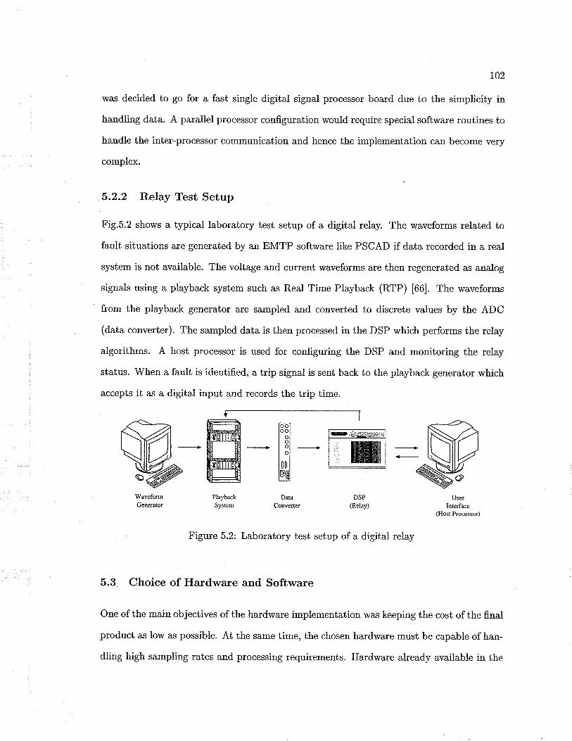
r02
was decided to go for a fast single digital signal processor board due to the simplicity in
handling data. A parallel processor configuration would require special software routines to
handle the inter-processor communication and hence the implementation can become very
complex.
5.2.2 Relay Test Setup
Fig.5.2 shows a typical laboratory test setup of a digital relay. The waveforms related to
fault situations are generated by an EMTP software tike PSCAD if data recorded in a real
system is not available. The voltage and current waveforms are then regenerated as analog
signals using a playback system such as Real Time Playback (RTP) [66]. The waveforms
from the playback generator are sampled and converted to discrete values by the ADC
(data converter). The sampled data is then processed in the DSP which performs the relay
algorithms. A host processor is used for configuring the DSP and monitoring the relay
status. When a fault is identified, a trip signal is sent back to the playback generator which
accepts it as a digital input and records the trip time.
WavefonnGenera(or
DSP(Relay)
Dâtâ
ConverterUser
Interface(Host Processor)
tffiM
Playback
System
FBI r@ -*;;;r+i,ir -@t!" I
PEI
Figure 5.2: Laboratory test setup of a digital relay
5.3 Choice of Ha¡dware and Software
One of the main objectives of the hardware implementation was keeping the cost of the final
product as low as possible. At the same time, the chosen hardware must be capable of han-
dling high sampling rates and processing requirements. Hardware already available in the
103
laboratory was examined first to assess their capabilities and identify the special hardware
and software requirements that could emerge when the two algorithms are combined. Once
the resources already available in the laboratory were found to be inadequate, alternatives
were considered. The configuration selected not only depends on the speed of the signal
processor, but also on the availability of data acquisition systems, user-friendliness of the
software and previous experience on the products from a particular manufacturer.
The sections to follow discuss the different configurations considered for the implemen-
tation of the relay prototype, and the reasons for the failure of some of them. Four different
configurations were tested during the development phase:
1. Spectrum Dakar board with DL3-41 ADC
2. Texas Instruments TMS320C6711 DSK with THS1206 ADC
3. Texas Instruments TMS320C671i DSK with TLV2548 ADC
4. Texas Instruments TMS320C6711 DSK with ADS8364 ADC
5.4 Spectrum Board Configuration
5.4.L Spectrum Dakar F5 Carrier Board
Spectrum Dakar F5 board [67] provided as a grant by the Canadian Microelectronics Cor-
poration (CMC) under a product evaluation program was considered as an option to imple.
ment the relaying algorithm. This board was used to identify the main requiremenis of the
real-time prototype. Dakar F5 is a configurable DSP platform based on Spectrum Signal
Processing Inc.'s Dakar boards and has an embedded Texas Instrument (TI) TMS320C44
processor [68]. The board is supported with Spectrum Signal Processing Inc.'s Software
Development Kit (SDK) [69]. The configuration utility tool box [70] was used to generate
configuration files for the DSP system. The code was generated using Texas Instruments
Code Composer Studio (CCS) integrated development environment (IDE) [71]. The CCS

r04
allows the users to edit, build, debug, profile and manage projects with its MS-Visual C+*like single unified environment [72].
Specifications for Dakar F5:
- Embedded TMS320C44 50MHz processor
- Up to 50 MFLOPS, 25 MIPS performance
- Scalability up to 4 parallel processors
- 2 general-purpose timers
- 6 channel DMA coprocessor
- lMByte SRAM memory for Node A embedded processor
- 32-bit PCI interface with 132 MBytes/s peak transfer rate
- L0 external COMM ports (8-bit parallel communication ports)
- JTAG real time debugging interface
- On-board DSP-LINKSIconnector module
- TlM-402compliant code boot-strapping through onboard EPROM
5.4.2 Spectrum DL3-AL
Choosing a signal acquisition system with six or more analog inputs and which could be
interfaced with the Dakar F5 boa¡d was challenging. Finally, Spectrum Signal Processing
Inc.'s DL3-41 DL3ADA100 Analog Module [73] was selected as the analog to digital con-
verter. This is an add-on board that connects to Dakar board via a DSP-LINK3 module
connection [7a]. The module acts as a slave on the DSP-LINK3 bus. The DL3-41 provides
four analog input channels and two analog output channels. The objective was to stack two
DL3-41 analog modules in parallel on the two DSP-LINK3 poris to obtain the six inputs.tOSp-l,lNXg is an open standard for 32-bit 40 MByte/s I/O interface from Spectrum Signal processing
Inc2TIM-40 modules defi¡e a family of DSP modules, based. on TMS320C4x processors, designed for use in
multiple DSP systems
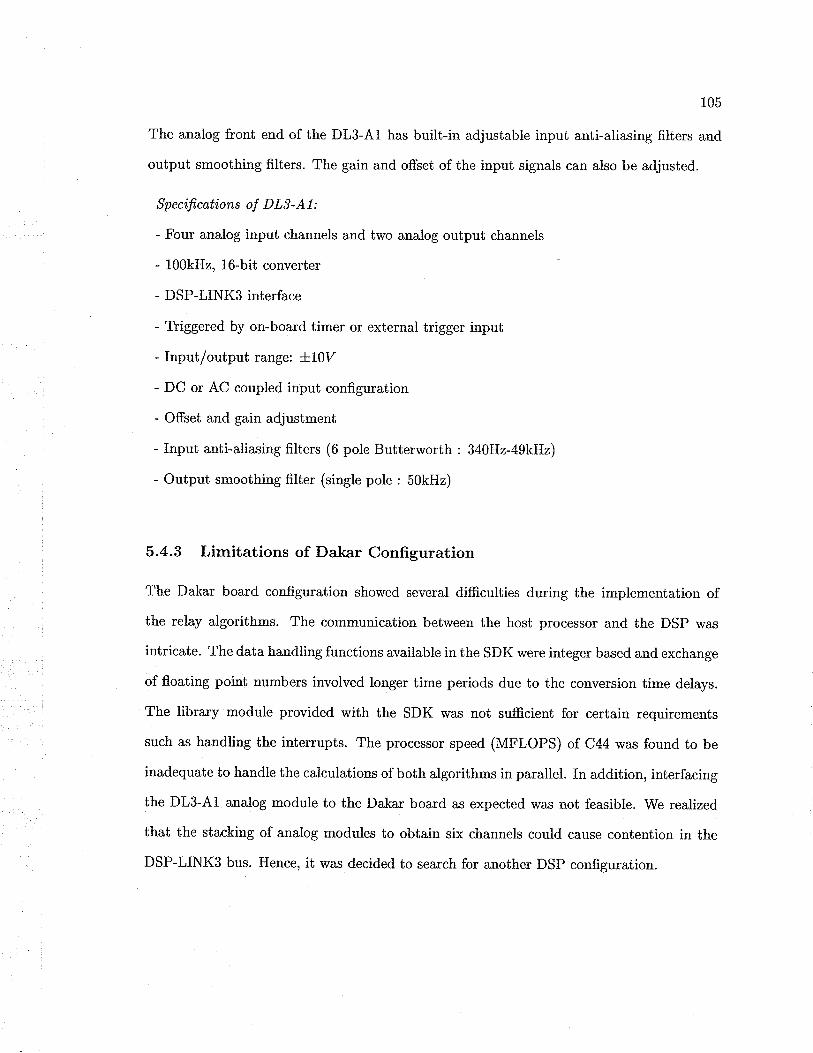
105
The analog front end of the DL3-Ai has built-in adjustable input anti-aliasing fiIters and
output smoothing filters. The gain and offset of the input signals can also be adjusted.
Speci,fi,cations of D L3- A I :
- Four analog input channels and two analog output channels
- 100kHz, 16-bit converter
- DSP-LINK3 interface
- Tliggered by on-board timer or external trigger input
- Input/output range: +10Y
- DC or AC coupled input configuration
- Offset and gain adjustment
- Input anti-aliasing filters (6 pole Butterworth: 340H2-49kHz)
- Output smoothing filter (single pole : 50kHz)
5.4.3 Limitations of Dakar Configuration
The Dakar board configuration showed several difficulties during the implementation of
the relay algorithms. The communication between the host processor anci the DSP was
intricate. The data handling functions available in the SDK were integer based and exchange
of floating point numbers involved longer time periods due to the conve¡sion time delays.
The library module provided with the SDK was not sufficient for certain requirements
such as handling the interrupts. The processor speed (MFLOPS) of. C44 was found to be
inadequate to handle the calculations of both algorithms in parallel. In addition, interfacing
the DL3-41 analog module to the Dakar board as expected was not feasible. We realized
that the stacking of analog modules to obtain six channels could cause contention in the
DSP-LINK3 bus. Hence, it was decided to search for another DSP configuration.
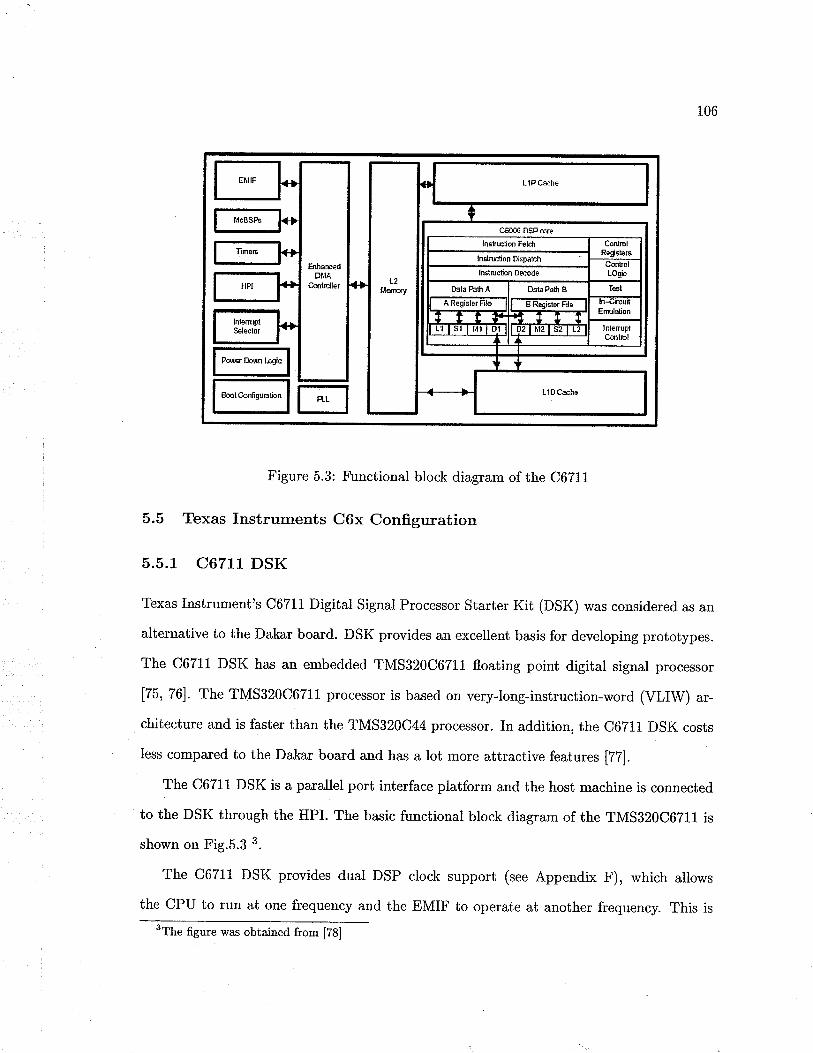
106
Êrharc¡dDt1À
Ctrlrdler L2Llemy
f-.*-.-ll'**,*l tr
Figure 5.3: F\rnctional block diagram of the C6TL1
5.5 Texas Instruments C6x Configuration
5.5.1 C67Lt DSK
Texas Instrument's C6711 Digital Signal Processor Starter Kii (DSK) was considered as an
alternative to the Dakar board. DSK provides an excellent basis for developing prototypes.
The C6711 DSK has an embedded TMS320C67Ll floating point digital signal processor
175,761. The TMS320C67I1" processor is based on very-long-instruction-word (VLIW) ar-
chitecture and is faster than the TMS320C44 processor. In addition, the C67II DSK costs
less compared to the Dakar board and has a lot more attractive features [77].
The C6711 DSK is a parallel port interface platform and the host machine is connected
to the DSK through the HPI. The basic functional block diagram of the TMSA20C6711 is
shown on Fig.5.3 3.
The C6711 DSK provides dual DSP clock support (see Appendix F), which allows
the CPU to run at one frequency and the EMIF to operate at another frequency. This is
3The figure was obtained from [78]

107
important in interfacing daughtercards to the DSP at data rates required by the application.
One of the McBSP ports is connected to an onboard codec and the other can be used to
interface a daughtercard connected to the expansion peripheral interface. The EDMA
controller is directly connected io the two McBSP ports and EMIF. This allows the EDMA
controller to control and access a daughtercard without interrupting the CPU, a very useful
feature that helps to reduce the workload of the CPU.
Speci,f,cations of C6711 DSK:
- 150 MHz clock speed
- Operating speeds up to 900 MFLOPS
- PPC interface to standard parallel port on a host PC (EPP or bi-directionat SPP)
- Eighi 32-bit instructions/cycle
- 6 ALU's and 2 multipliers
- 16MB of 100MHz SDRAM
- 32-bii external memory interface (EMIF)
- 16-bit host-port interface (HPI) access to all DSP memory
- 16 EDMA channels with simultaneous data handling capabilities
- 2 multi-channel buffered serial ports (McBSP)
- 2 general-pupose timers
- Phase.locked-loop (PLL) clock generator
- 128K8 of EPROM
- HPI and 32-bit ROM booi modes
- L1,/L2 memory architecture
- 16-bit audio codec
- Expansion memory and peripheral connectors for daughterboard support
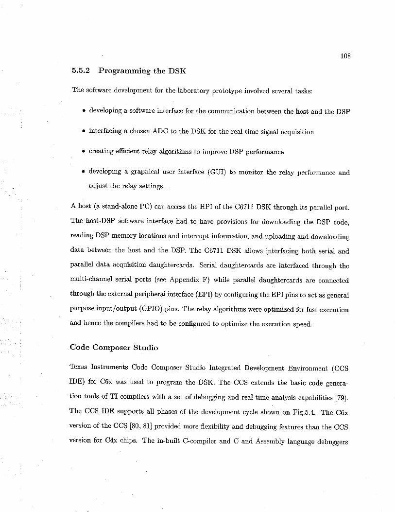
108
5.5.2 Programming the DSK
The software development for the laboratory prototype involved several tasks:
o developing a software interface for the communication between the host and the DSP
o interfacing a chosen ADC to ihe DSK for the real time signal acquisition
o creating efficient relay algorithms to improve DSP performance
o developing a graphical user interface (GUI) to monitor the relay performance and
adjust the relay settings.
A host (a stand-alone PC) can access the HPI of the C6711DSK through its parallei port.
The host-DSP software interface had to have provisions for downloading the DSP code,
reading DSP memory locations and interrupt information, and uploading and downloading
data between the host and the DSP. The C6711 DSK allows interfacing both serial and
parallel data acquisition daughtercards. Serial daughtercards are interfaced through ihe
multi-channel serial ports (see Appendix F) while parallel daughtercards are connected
through the external peripheral interface (EPI) by configuring the EPI pins to act as general
purpose input/outpui (GPIO) pins. The relay algorithms were optimized for fast execution
and hence the compilers had to be configured to optimize the execution speed.
Code Composer Studio
Texas Instruments Code Composer Studio Integrated Development Environment (CCS
IDE) for C6x was used to program the DSK. The CCS extends the basic code genera-
tion tools of TI compilers with a set of debugging and real-time analysis capabilities [7g].
The CCS IDE supports all phases of the development cycle shown on Fig.5.4. The C6x
version of the CCS [80, 81-] provided more flexibility and debugging features than the CCS
ve¡sion for C4x chips. The in-built C-compiler and C and Assembly language debuggers
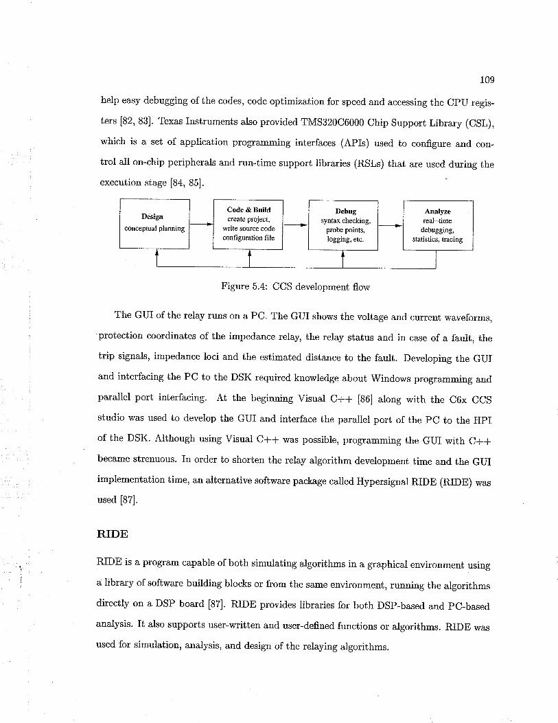
109
help easy debugging of ihe codes, code optimization for speed and accessing the CPU regis-
ters [82, 83]. Texas Instruments also provided TMS320C6000 Chip Support Library (CSL),
which is a set of application programming interfaces (APIs) used to configure and con-
trol all on-chip peripherals and run-time support libraries (RSLs) that are used during the
execution stage [84, B5].
Figure 5.4: CCS development flow
The GUI of the relay runs on a PC. The GUI shows the voltage and current waveforms,
protection coordinates of the impedance relay, the relay status and in case of a fault, the
trip signals, impedance loci and the estimated distance to the fault. Developing the GUI
and interfacing the PC to the DSK required knowledge about Windows programming and
parallel port interfacing. At the beginning Visual C++ [86] along with the C6x CCS
studio was used to develop the GUI and interface the parallel port of the PC to the HpI
of the DSK. Although using Visual C++ was possible, programming the GUI with C++
became strenuous. In order to shorten the relay algorithm development time and the GUI
implementation time, an alternative software package called Hypersignal RIDE (RIDE) was
used [87].
R,IDE
RIDE is a program capable of both simulating algorithms in a graphical environment using
a library of software building blocks or from the same environment, running the algorithms
directly on a DSP board [87]. RIDE provides libraries for both DSP-based and pC-based
analysis. It also supports user-written and user-defined functions or algorithms. RIDE was
used for simulation, analysis, and design of the relaying argorithms.
Code & Buildcreate project,
write source codeconfiguration file

110
We used a component based approach in developing relaying algorithms which was
supported by RIDE. This was accomplished by the utilizaiion of dynamic link libraries
(DLLs) that were designed to run with RIDE. These DLLs (or biock DLLs) were designed
to do specific tasks. The blocks were then connected together according to the data flow
between them. Only the required componen{s that were not included in the standard library
of general blocks and the standard library of DSP blocks of RIDE [88] were additionally
created. Each created block has two pa.rts associated with ii; a DLL file that runs on the
host and an object code that runs on the DSP. The block DLL is responsible for data t¡ansfer
from the host to the DSP. The host program or the DLL was created using Microsoft Visual
C++ version 6.0 [89]. To create the object code that runs on ihe DSP, C6x CCS was used
[80].
To create the relaying algorithms using RIDE, the real-time function blocks were ar-
ranged according to the requirements of the algorithm on a worksheet under the RIDE
graphical user environment. The function blocks were connected to establish the data flow
and then the parameters of the blocks were set. The parameters were selected to set DSP
resources and handle synchronization, interrupt, and profile configurations. The real-time
block functions in a worksheet communicate with the DSP board driver and other blocks to
transmit data flow information. The DSP board driver performs the linking of DSP object
files, downloads code, data, and parameters to DSP memory, controls the execution of the
DSP, monitors DSP activit¡ and provides DSP resource allocation information.
5.5.3 Choice of Analog to Digital Converters for C67LL DSK
To acquire the three voltage and three current signals required for the relay algorithm,
an analog to digital converter having six or more channels, which can be interfaced with
the C6711 DSK, had to be chosen. Texas Instruments provided several daughterboards
which could be directly interfaced with the C67i1 DSK through the EMIF and peripheral
connecter [90]. However, at the time the search for ADCs started, it was not possibie io find

111
a unit with six or more channels from the selection of TI daughterboards. Hence, third-party
companies had to be sought for their products which satisfied the above requirements. The
cheapest solution that could be found ihrough web search was Signalware Corporation's
AED-106 board. In this board, four Texas Instruments THS1206 data converters [g1] were
multiplexed in a single configuration and hence provided 16 analog inputs and 24 digital
I/O. However, AED-106 was considered expensive for this implementation. That could have
made the overall cost of the relay high. Thinking along the design of the AED-106, it was
decided to use THS1206 for data acquisition.
5.6 THS1206EVM Analog to Digital Converter
THS1206 is a four channel l2bit 6MSPS simultaneous sampling data converter. An inte-
grated L6 word deep FIFO allows the storage of data in order to take the load off of the
processor connected to the ADC [92]. Fast data throughput is achieved with the integrated
FIFO.
Specif,cati.ons of T H S 1 20 6 E VM :
- High-Speed 6MSPS ADC
- 12-bit resolution
- 4 single-ended or 2 differential inputs
- Simultaneous sampling channels
- 16 word, 12-bit integrated FIFO
- Parallel glueless p,C/DSP interface
The block diagram of the THS1206 with the inputs and outputs is shown in Fig.5.5 a.
The THS1206EVM has a parallel interface and is connected to the C67It DSK th¡ough the
common connector interface [78]. Interfacing an ADC having a parallel interface to a DSP
can become complex compared to an ADC equipped with a standard serial interface andaThe figure obtained from [g1]

7t2
ov.ooa:________
| *rro*
DATÂ_¡{V
BVoo
DO
BIÐ2D3t]4D5Ð6tîtsBgol0,rRA0ûl1nA't
BGI,ID
BINTü
co¡¡v clxtffii)ESoCST
EÚffi'tnfit
¡ ---------rAGND
Figure 5.5: THS1206 block diagram
usually there are many ways to build the interface. fn our implementation, the read and
write inputs (RD, WR) and the programmable control signal DATA-AV were used to read
the data from the THS1206 to the DSK [93]. Fig.5.6 shows the signals associated with the
connection of EVM to the DSK.
In order to program the THS1206 into the desired mode, two 10-bit wide internal control
registers (CR0, CRl) were used. Several steps had to be followed to program the registers.
The THS1206 was reset at the beginning of initialization by writing 0x401 to CRl. Then
the reset was cleared by writing 0x400 to CRl. The user configuration required for sampling
four channels was written to CRO and CRl after that. The write access was required to
reset and configure the THS1206 to the desired operation mode. The read access transferred
converted samples from the THS1206 to the DSP. The conversion clock was generated by
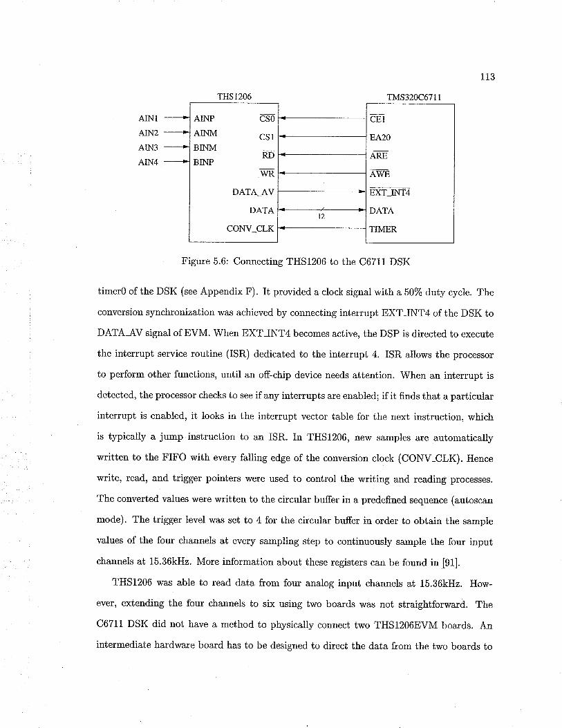
113
THS 1206
AINI
AIN2
AIN3
AiN4
Figure 5.6: Connecting THS1206 to the C67i1 DSK
timerO of the DSK (see Appendix F). It provided a clock signal with a 50% duiy cycle. The
conversion synchronization was achieved by connecting interrupt EXTINT4 of the DSK to
DATA-AV signal of EVM. When EXTINT4 becomes active, the DSP is directed to execute
the interrupt service routine (ISR) dedicated to the interrupt 4. ISR allows the processor
to perform other functions, until an off-chip device needs attention. When an interrupt is
detected, the processor checks to see ifany interrupts are enabled; ifit finds that a particular
interrupt is enabled, it looks in the interrupt vector table for the next instruction, which
is typically a jump instruction to an ISR. In THS1206, new samples are automatically
written to the FIFO with every falling edge of the conversion clock (CONV-CLK). Hence
write, read, and trigger pointers were used to control the writing and reading processes.
The converted values were written to the circular buffer in a predefined sequence (autoscan
mode). The trigger level was set to 4 for the circular bufier in order to obtain the sample
values of the foul channels at every sampling siep to continuously sample the four input
channels at 15.36kH2. More information about these registers can be found in [91].
THS1206 was able to read data from four analog input channels at 15.36kH2. How-
ever, extending the four channels to six using two boards was not straightforwa^rd. The
C67I7 DSK did not have a method to physically connect two THS1206EVM boards. An
intermediate hardware board has to be designed to direct the data from the two boards to
AINP CSO
AINM CSIBINM
RDBINP
_mDATA_AV
DATA
CONV-CLK
CEI
EA2O
ARE
ewp
EXT-ñ4
DATA
TIMER

174
the DSK. To do that, the timing of the DATA-AV signals from the two boards has to be
synchronized properly to read the data sampled at the same instant. The DATA-AV signal
has to control the data bus to avoid possible bus contentions. Considering all these factors,
it was decided to discard the idea of using THS1206EVM and move onto a data converter
board with six or more input channels.
At the time of the decision, we could not find a data converter having six or more
channels, which could be directly interfaced with the C6711DSK from Texas Instrument
or any of their third party hardware manufacturers. However, we realized that Texas
Instruments TLV2S4BEVM with eight analog input channels could be interfaced to the
C6711DSK with the use of an off-the-shelf intermediate adaptor board.
5.7 TLV2548EVM Analog to Digital Converter
TLV2548EVM is a 12-bit analog-to-digital converter (ADC) with eight analog input chan-
nels, an 8-level FIFO, and four different conversion modes [g4].
S pecif,cati,ons of T LV 2 5 /¡ I E VM :
- Maximum throughput 200-KSPS
- 12-bit resolution
- Built-in reference, conversion clock and SxFIFO
- DSP-compatible serial interface with SCLK up to 20-MHz
- Hardware controlled and programmable sampling periods
- Programmable auto-channel sweep
The ADC can be interfaced to the C6711DSK using the Multichannel Buffered Serial
Port (McBSP) of the DSP. The EVM has three digital inputs and a 3-state output [chip
seleci (CS), serial input-output clock (SCLK), serial data input (SDI), and serial data output
(SDO)] that provide a direct 4-wire interface to the serial port. A frame sync (FS) signal
is used to indicate the start of a serial data frame. The sample-and-hold function can be

controlled by a special pin, CSTART if required.
is shown in Fig.5.7 5.
115
F\rnctional block diagram of the TLV2548
eocrjffi
Figure 5.7: TLV2548 functional block diagram
The TLV2548EVM can be directly interfaced with the Texas Instruments TMSB20C54x
type DSKs [96], but cannot be directly connected to the C6711DSK [97]. In C6211 DSK,
two 80-pin headers are used to bring signals to the daughtercards. One of the headers
is primarily used for peripheral signals while the other is primarily used for the external
memory interface (EMIF). The daughtercard interface on the DSP motherboard has several
set requirements concerning signal drive, timing delay, and voltage tolerance [g8]. lVhen a
daughtercard is connected to a DSP, these requirements have to be satisfied. TLV2548 has
a serial interface. Most currently-used data converter EVMs that feature a serial interface
use the first serial port (McBSPl) when interfacing to the DSP. The 80-pin EPI header
REFP
REFÍII
zs¿e ìï,0-- |illÂ3çA4t
trJsDr
cMR{4 MSSS}
GNÐ
sThe figure obtained. from [9b]

TLV2548 SPRATI I
116
TMS320C6711
AINI
AIN2
AIN3
AIN4
ATN5
AIN6
AINT
AINS
Figure 5.8: Connection between TLV2548EVM and C67L1DSK
on the DSK provid.es access to McBSPl, but TLV2548EVM is not compatible with this
interface. Hence an off-the-shelf adaptor board, SPRA711, provided by Texas Instruments
was selected and modified to interface the signals between the EVM and the DSK.
The SPRA711 [99] is a cross-platform daughtercard adapter board designed to be used
in conjunction with the data converter EVM's from Texas Instruments. This allows daugh-
tercards designed for one motherboard to be used on the others. The interface is developed
according to the TMS320 Cross-Platform Daughtercard Specification [98]. The interface
provides a serial interface to the daughtercard. The C6711 DSK provides two 7-signai se-
rial ports to the daughtercard. This includes clock (CLKX, CLKR), frame (FSX, FSR),
and data signals for both the transmit and receive data streams, as well as a clock input
to operate the serial port asynchronously to the DSP. In addition, the adaptor board aI-
lows the daughtercard to access the two timer outputs (TOUT), external interrupt signals
(EXT_INT), and other general purpose input/output (I/O) signals. Of the two serial in-
terfaces present on the DSK, one is dedicated to the daughtercard and one is selectable
between the daughtercard and system hardware. With switches available on the DSK, the
McBSP port used to access the daughtercard can be chosen. In this design, McBSP port Iwas used.
A1
A2
A3
A4
A5
A6
A7
A8
CLKX
CLKR
FSX
FSR
EVM_DXa
EVM_DRa
EVM_CLKXa
EVM_CLKRa
EVM_FSXa
EVM_FSRa
EVM_INTa
DC CNTLa
DXI
DRI
CLKXI McBSPICLKRI
FSXl
FSRl

LTT
Fig.5.8 shows how the TLV2548EVM was connected to the C671lDSK through the
SPRA711. The McBSP drives serial-line transmit clock CLKX and transmit frame sync
FSX signals, and accepts receive clock CLKR and receive frame sync FSR signals as inputs.
Serial lines CLKX and CLKR, as well as FSX and FSR, are connected together on the
TLV2548EVM. An interrupt signal is issued by the EVM at the end of each conversion.
The TLV2548 interrupt line was tied to INT4 of the DSP [100] in our application. A low
sampling rate (1920H2) was attempted at the beginning and it was increased to a higher
value (15.36kH2) Iater.
The McBSP was used to generate the required clock pulses for the conversion using the
sample rate generator (SRG) (see Appendix F). The SRG is composed of a tbree.stage
clock divider that allows programmable daia clocks (CLKG) and framing signals (FSG).
These McBSP internal signals were programmed to drive receive and transmit clocking
(CLKR/X) and framing (FSR/X). The sample rate generator register (SRGR) controls the
operation of the various functions of the SRG. The transmit control register (XCR) and
receive control register (RCR) were programmed to set the mode of the transmitter and
receiver. The McBSP had to be initialized in order to use it as a serial bufier [101]. Fig.5.g
shows the sequence in which the McBSP serial port was initialized and how the TLV2548
\¡/as programmed to sample six analog input channels. Different steps and the register
contents associated with each step are described in sequence.
In the step 1-, EXTINT4 was enabled and assigned to the ISR associated with reading
data from the EVM. In the next step, the McBSPI was initialized. The transmitter, the
receiver, the frame-sync generator, and the sample rate generator rilere first disabled by
asserting the serial port reset state (MCBSPI-SPCR : 0x0). The McBSP configuration
registers were programmed while the serial port was in the reset state. The pin control
register (McBSPIfCR), receive control register (McBSPl-RCR), transmit control register
(McBSPIJCR), and sample rate generator register (McBSPI-SRGR) of serial port 1 were
programmed as follows:
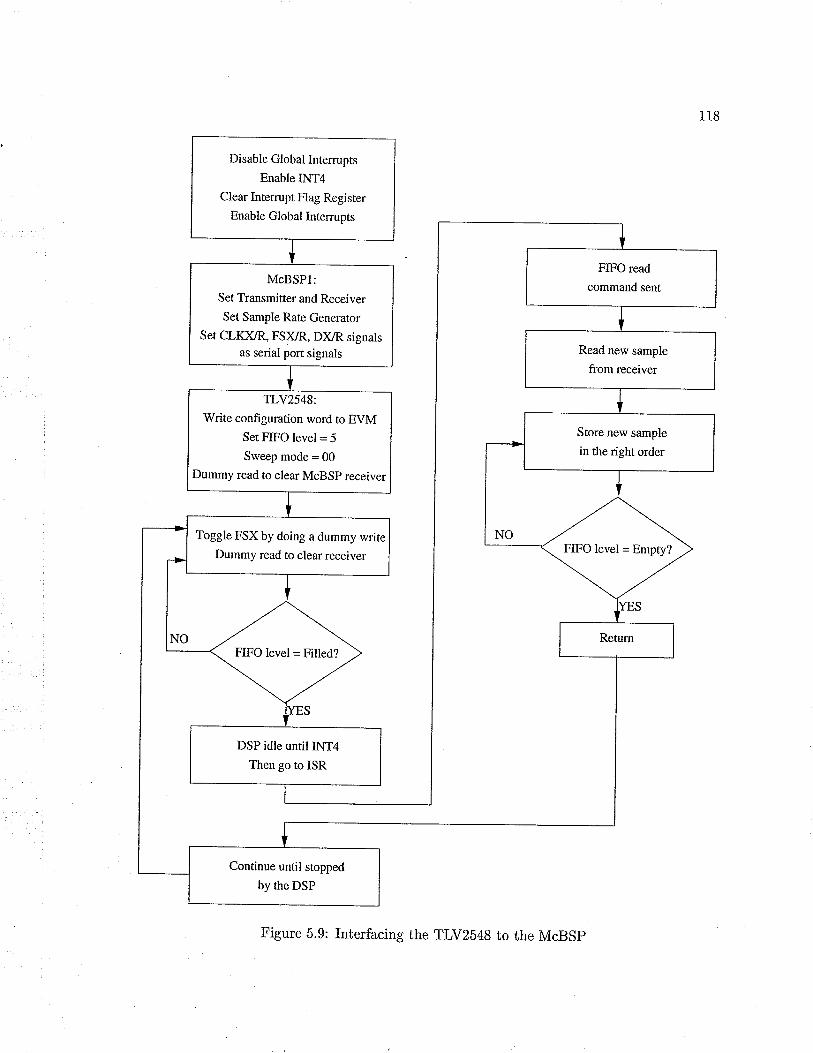
118
Disable Global Interrupts
Enable INT4Clear Interrupt Flag Register
Enable Global Intemrpts
FIFO read
command sentMcBSPI:
Set Transmitter and Receiver
Set Sample Rate Generator
Set CLK)IR, FSX/R, DX/R signalsas serial port signals Read new sample
from receiver
TLY2548:
Write configuration word to EVMSet FIFO level = 5
Sweep mode = 00
Dummy read to clear McBSp receiver
Store new sample
in the right order
FIFO level = Empty?Toggle FSX by doing a dummy write
Dummy read to clear receiver
FIFO level = Filled?
DSP idle until INT4
Then go to ISR
Continue until stopped
by the DSP
Figure 5.9: Interfacing the TLVZ548 to the McBSp

119
McBSPI-PCR : 0x00000400:
. DX, FSX, CLKX are serial-port pins
r DX is the data-transmit pin
o FSX is the frame-sync pin, and is driven by the SRG
o FSR is an input pin driven by an external source
e CLKX is an output pin driven by the internal SRG
¡ CLKR is an input pin driven by an external clock
¡ FSX and FSR are active high
¡ The transmit data is sampled on the rising edge of CLKX
o The receive data is sampled on the falling edge of CLKR
McBSPI-RCR : 0x00420040:
¡ Receive one 16-bit word per frame
o Single phase - only one data word per FSR
¡ Last four LSBs are zero-padded
o Data transfer to start with the MSB
o l-bit data receive delay
¡ Data sent out by ADC immediately after FSR fatling edge
McBSPI-XCR : 0x00420040:
o Thansmit one 16-bit word per frame
o Single phase - only one data word per FSX
L20
o Last four LSBs are zero-padded
o Data transfer to start with MSB first
r l-bit data transmit delay
¡ Data sent to ADC immediately after FSX
McBSPI-SRGR : 0x301C0111:
. SRG clock is derived from the internal clock
¡ FSX is driven by the SRG clock
o Fbame-sync pulse width (FWID) : 1 CLK period
o SCLK : (CPU clock f (l+CLKGDV)). Desired SCLK :6.25MH2. Since the CPU
clock is equal to 75 MHz, CLKGDV : 11 to generate the required SRG clock frequency
¡ To generate the required frame sync (FSG :2I5.5kHz), FPER : 28
After setting the McBSPI registers, the transmitter, the receiver, the frame-sync gen-
erator, and the sample rate generator were enabled (McBSPI-SPCR : 0x0C50023).
The next step was configuring the TLV2548EVM. TLV2548 can be controlled by writing
a 16-bit word through SDI. Different commands can be used to select the channels, read
data from the EVM configuration register (CFR), write values to CFR or read data from
the FIFO. TLV2548 uses the first 4 bits as command bits. Table 5.1 shows the command
set associated with the TLV2548.
The EVM is configured at initialization by writing the first bits as OxA and the follow-
ing 12 bits contain the configuration data. Table 5.2 shows the configuration register bit
deûnitions.
To read the six channels continuously from the ADC, the CFR was programmed as
follows:

r21
sDr [15-12] COMMAND
0000
0001
0010
0011
0101
0110
0111
1000
1001
1010
101 1
1100
1101
1110
1111
Select analog input channel 0
Select analog input channel 1
Select analog input channel 2
Select analog input channel 3
Select analog input channel 5
Select analog input channel 6
Select analog input channel 7
SW power down (analog * reference)
Read CFR register data shown as SDO D[i1 - 0]
Write CFR followed by 12-bit data
Select test, voltage : (REFP+REFM)/2
Select test, voltage : REFM
Select test, voltage : REFP
FIFO read, FIFO contents shown as SDO DllS - 41,
Reserved
Dlï-01 :0000
TLV254B-CFR : 0xA8C1:
o fnternal 4V reference voltage
r Short sampling
o Conversion clock source : SCLK
o Sweep mode
o Sweep auto sequence 0-L-2-3-4-5-6-7
r EOC/INT pin used as INT
o FIFO trigger levelSl4 (for six channels)
The EXTINT4 of ihe DSP was used to serve the interrupt signal issued by the EVM
when the FIFO trigger level was reached.
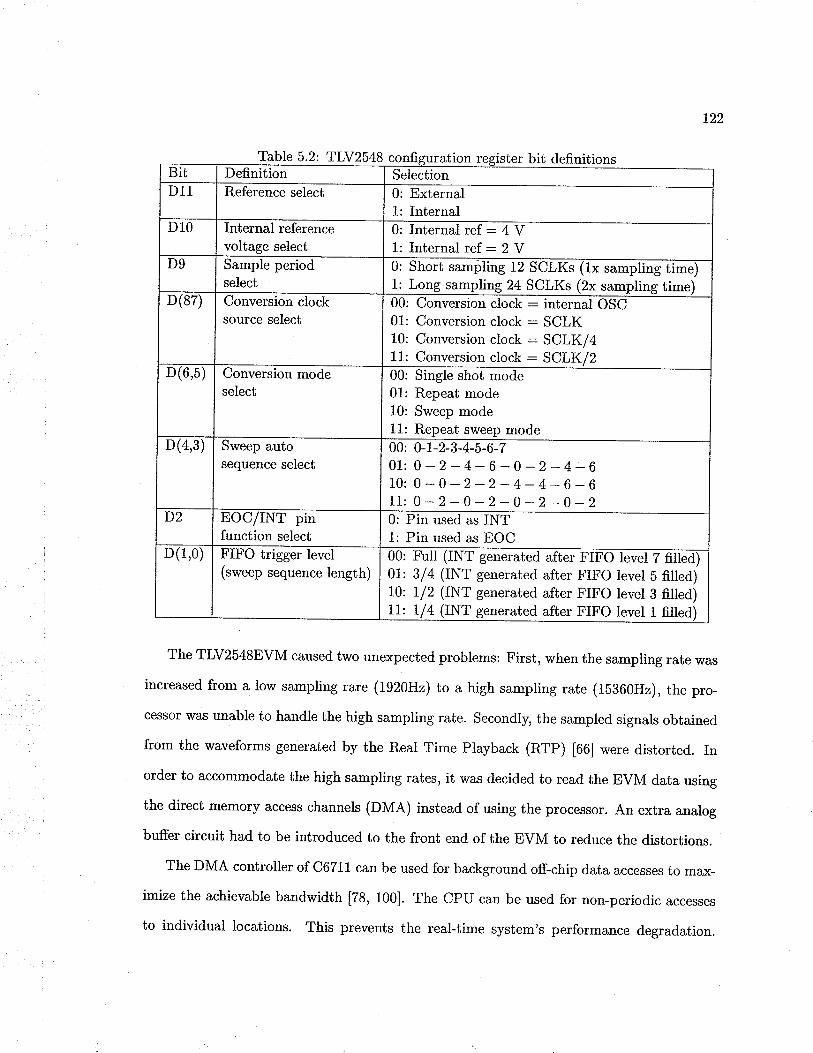
I22
Table 5.2: TLY2548 ration ister bit definitionsBir Definiiion SelectionD11 Reference select External
Internal0:1:
D10 Internal referencevoltage select
0: Internal ¡ef: 4 V1: Internal ref: 2 V
D9 Sample periodselect
0: Short sampling 12 SCLKs (1x sampling ti:ne)L: Long sampling24 SCLKs (2x sampling time)
D(87) Conversion clocksource select
00: Conversion clock : internal OSC01: Conversion clock : SCLK10: Conversion clock : SCLKI411: Conversion clock : SCLK12
D(6,5) Conversion modeselect
00: Single shot mode01: Repeat mode10: Sweep mode11: Repeat sweep mode
D(4,3) Sweep autosequence select
00: 0-1-2-3-4-5-6-701: 0 - 2 - 4 - 6 - 0 - 2 - 4 - 610:0-0-2-2-4-4-6-611:0-2-0-2-0-2-0-2
D2 EOC/INT pinfunction select
0: Pin used as INT1: Pin used as EOC
D(1,0) FIFO trigger level(sweep sequence length)
Fbll (INT generated after FIFO level 7 ñlled3/4 (INT generated after FIFO level 5 filled)i/2 (INT generated after FIFO level 3 filled)1/4 (INT generated after FIFO level 1 filled)
00:
01:
10:
11:
The TLV2548EVM caused two unexpected problems: First, when the sampling rate was
increased from a low sampling rare (1920H2) to a high sampling rate (1b360H2), the pro-
cessor was unable to handle the high sampling rate. Secondly, the sampled signals obtained
from the waveforms generated by the Real Time Playback (RTP) [66] were distoried. In
order to accommodate the high sampling rates, it was decided to read the EVM data using
the direct memory access channels (DMA) instead of using the processor. An extra analog
buffer circuit had to be introduced to the front end of the EVM io reduce the distortions.
The DMA controller of C6711 can be used for background off-chip data accesses to max-
imize the achievable bandwidth [78, 100]. The CPU can be used for non-periodic accesses
to individual locations. This prevents the real-time system's performance degradation.
723
Although the CPU and the DMA controller function independently of one another, it is
necessary to properly schedule and configure them in order to minimize conflict and waiting
while meeting real-time requirements. After referring to several application notes from the
Texas Instruments [96, 103, 104] and attempting to program the DMA to read from the
TLV2548, we realized that the DMA cannot access six different channels at the same time in
the sweep mode. The DMA could access the six channels under single-shot mode by reading
one channel at a time and then rotating between the channels. However, this method did
not achieve the high sampling rates required due to latency involved in switching between
channels. Hence the idea of improving the data transfer speed through the DMA had to be
abandoned.
During this period, Texas Instruments introduced the 4DS8364, a ne\¡/ ADC EVM
with six analog input channels which could be directly interfaced to the C6711DSK. Due
to the difficulties associated with interfacing the TLV2548EVM, it was decided to use the
ADS8364EVM to acquire the voltage and current signals.
5.8 ADS8364EVM Analog to Digital Converter
The ADS8364 is a high-speed, 6-channel, 250kHz, simultaneous sampling parallel ADC
with the 6 channels grouped into three pairs for high-speed simultaneous signal acquisition.
ADS8364EVM can be directly connected to the C671lDSK through the 80-pin interface
connectors [105].
The ADS8364 contains six 16-bit ADCs that can operate simultaneously in pairs. The
three hold signals (HOLDA, HOLDB, and HOLDC) initiate the conversion on the specific
channels. A simultaneous hold on all six channels can occur with all three hold signals
strobe together. The converted values are saved in six registers. For each read operation,
the ADS8364 outputs 16 bits of info¡mation. The Address/Mode signals (40, ,{1, and A2)
select how the data is read from the 4DS8364. These Address/Mode signaìs can define a
selection of a single channel, a cycle mode that cycles through all channels, or a FIFO mode
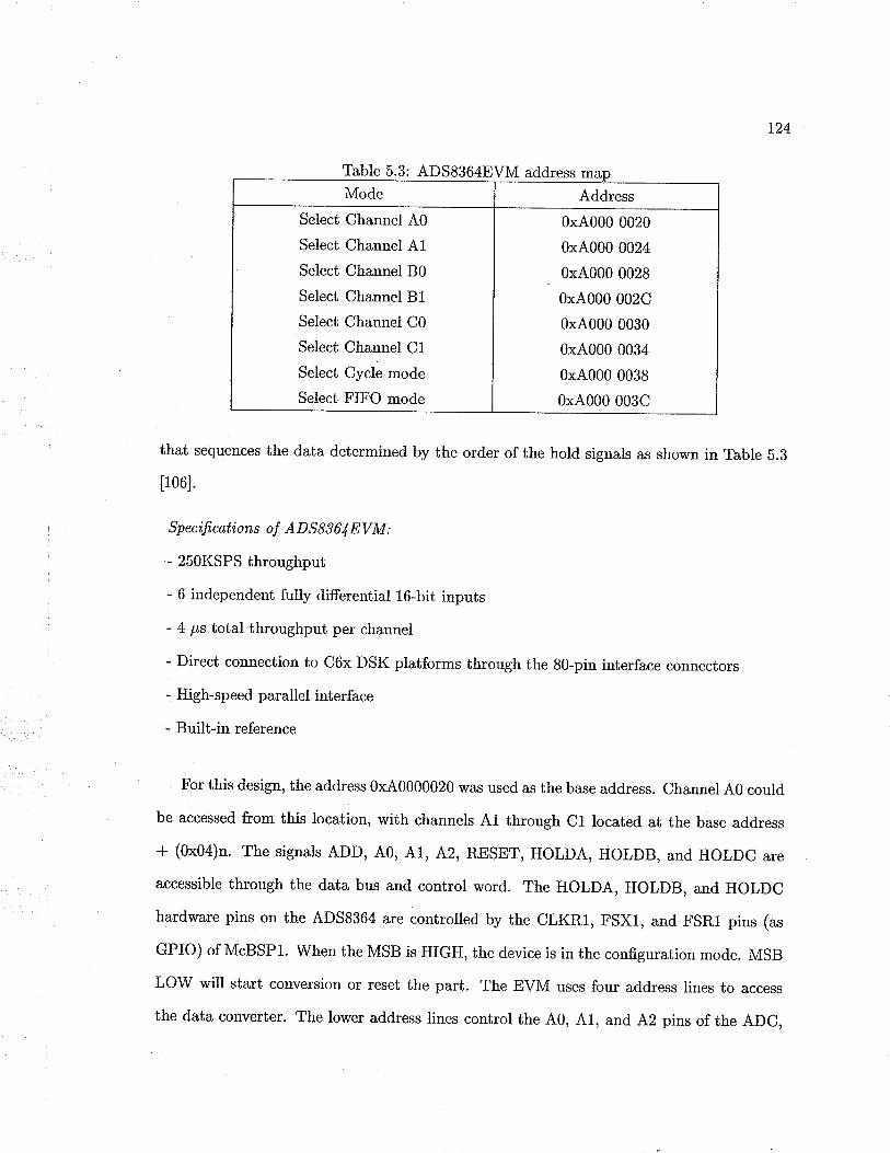
L24
Table 5.3: ADS8364EVM address
Mode Address
Select Channel A0
Select Channel A1
Select Channel B0
Select Channel B1
Select Channel C0
Select Channel ClSelect Cycle mod.e
Select FIFO mode
0x4000 0020
0x4000 0024
0x4000 0028
0x4000 002C
0x4000 0030
0x4000 0034
0x4000 0038
0x4000 003C
that sequences the data determined by the order of the hold signals as shown in Table 5.8
[106].
Speci,fi.catí,ons of A D S 83 6lEV M :
- 250KSPS throughput
- 6 independent fully differential 16-bit inputs
- 4 ps total throughput per channel
- Direct connection to C6x DSK platforms through the 80-pin interface connectors
- High-speed parallel interface
- Built-in reference
For this design, the address 0x40000020 was used as the base address. Channel A0 could
be accessed from this location, with channels A1 through C1 located at the base address
+ (0x04)n. The signals ADD, 40, 41, 42, RESET, HOLDA, HOLDB, and HOLDC are
accessible through the data bus and control word. The HOLDA, HOLDB, and HOLDC
hardware pins on the ADS8364 are controlled by the CLKRI, FSXI, and FSR1 pins (as
GPIO) of McBSPl. When the MSB is HIGH, the device is in the configuration mode. MSB
LOW will siart conversion or reset the part. The EVM uses four address lines to access
the data converter. The lower address lines control the 40, 41, and A2 pins of ihe ADC,
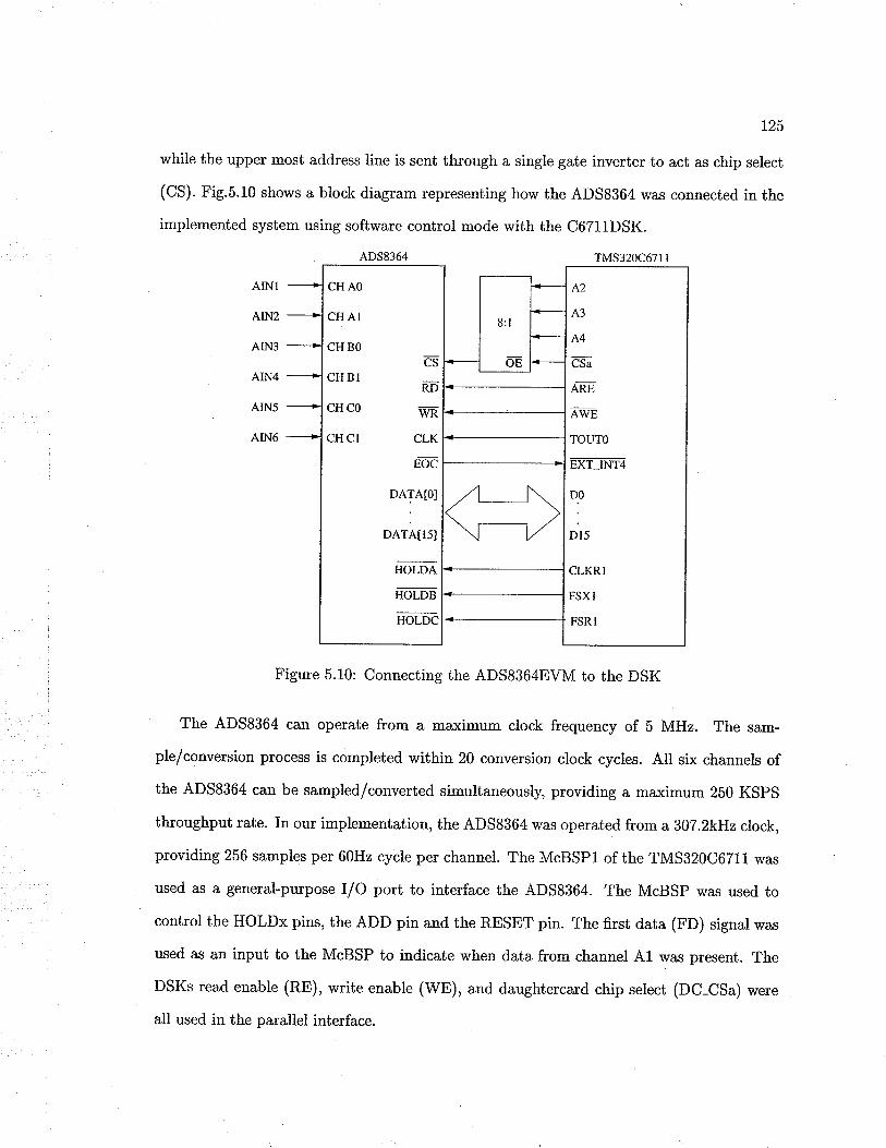
125
while the upper most address line is sent through a single gate inverter to act as chip select
(CS). Fig.5.L0 shows a block diagram representing how the ADS8364 was connected in the
implemented system using software control mode with the C6Z11DSK.
ADS8364 TMS320C67t I
AINl
AIN2
AIN3
AIN4
AIN5
AIN6
Figure 5.10: Connecting the ADS8364EVM to the DSK
The ADS8364 can operate from a maximum clock frequency of 5 MHz. The sam-
ple/conversion process is completed within 20 conversion clock cycles. Alt six channels of
the ADS8364 can be sampled/converted simultaneously, providing a maximum 250 KSPS
throughput rate. In our implementation, the ADS8364 was operated from a 307.2kH2 clock,
providing 256 samples per 60Hz cycle per channel. The McBSPI of the TMS320C6711 was
used as a general-purpose I/O port to interface the 4DS8364. The McBSP was used to
control the HOLDx pins, the ADD pin and the RESET pin. The first data (FD) signal was
used as an input io the McBSP to indicate when data from channel A1 was present. The
DSKs read enable (RE), write enable (WE), and daughtercard chip select (DC-CSa) were
all used in the parallel interface.
CH AO
CH AI
CH BO
esCHBI
RD
CHco WR
CHCI CLK
rõõ
DATA[0j
DATAI15j
A2
A3
A4
CSa-
ARE
-AWETOUTO
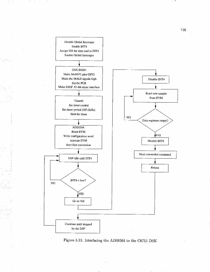
126
Disable Global Intemrpts
Enable INT4
Assign ISR for data read ro INT4
Enable Global Intemrpts
DSK EMIF:
Make McBSPI pins GPIO
Make the HOLD signals high
Set the PCRMake EMIF 32-bit async inrerface
NO
Disable fNT4
Read new sample
from EVMTimerO:
Set timer control
Set timer period (307.2kH2)
Start the timer
Data registers empry?
ADS8364:
Reset EVM
Write configuration word
Activate EVM
Start first conversion
Next conversion comma¡dDSP idle until INT4
Continue until stopped
by the DSP
Figure 5.11: Interfacing the ADS8364 to the C6211 DSK
r27
The different steps involved in interfacing the ADS8364EVM io the DSK are shown in
Fi9.5.11. In the first step, the external interrupt 4 of the processor was assigned to the
ISR that handles reading data from the EVM. The EOC signal is active low once for each
channel pair converted and in our implementation the EOC signal was routed to EXTINT4
on the C67LI DSK. In the next step, the McBSPI pott on the DSK was confi.gured. as a
general-purpose I/O port. To set up McBSPI as a GPIO port SRGR and SPCR were
cleared (McBSPI-SRGR : 0x0; McBSPI-SPCR : 0x0) and then, pCR was set for the
desired functions:
McBSPIfCR : 0x3F0F:
¡ FSX is a general purpose I/O
o FSR is a general purpose I/O
r CLKX is a general purpose I/O
¡ CLKR is a general purpose I/O
¡ DX is a general purpose output
o DR is a general purpose input
o HOLDx lines are set
o ADD line is cleared
In the next step, the conversion clock was set. The DSKs internal timer, TOUTg, was
used as the conversion clock source for the ADS8364EVM. The clock was set for 50/50 duty
cycle and a division multiple of 244. This provided approximately a J}T.2kHz conversion
clock to the conve¡ter.
The last step of ihe initialization was configuring the EVM. The data inputs and com-
mands associated with the EVM are given in Table 5.4. The commands are set by writing
to the base address of the ADC (ADC-BASE). First ihe ADS8364 was reset to ensu¡e that

128
Table 5.4: ADS8364 data input/commandCommand D7 D6 D5 D4 D3 D2 D1 DO
Convert 0 X RESET HOLDA HOLDB HOLDCConfiguration 1 X BIN/2s ADD
^2A1 AO
the read pointer was pointing to the first data register (ADC3ASE : 0x0002). The EVM
was then configured for continuous data sampling in CYCLE mode and binary data output
format (ADC3ASE : 0xg0). The EVM was then activated and first conversion command
was issued to sample all six channels (ADC_BASE : 0x04).
The HOLDx hardware pins are active low sampling triggers. When the three HOLD
lines are brought low together, all six analog inputs are simultaneously sampled and the
conversion process begins with the next rising clock edge. The conversion results are auto-
matically stored in the data registers starting with channel ,{0. The conversion is completed
after 20 clock cycles, at which time the end of conversion (EOC) pin goes low for I 12 clock
cycle on all three channels. When EOC is detected, the ISR is activated and the sampled
data values are read from the EVM. When all six channels have been read, the EVM is
issued the next conversion (HOLDx) command. To get the maximum throughput from the
4DS8364, ihe HOLDx command was set to be issued prior to reading the contents of the
data registers. This allows the ADC to start a new conversion sequence while the host
processor reads the results of the current conversion. ISR makes sure that the read process
is completed before the new conversion cycle is finished.
The ADS8364EVM solved the problems associated with capturing voltage and current
signals to the C67I1DSK. Several difficulties associated with the three EOC commands
had to be solved before the required sampling rate of 15.36kH2 could be achieved.
L29
5.9 Hybrid Algorithm fmplementation
The C6711 DSK provided a feasible, but inexpensive platform to implement the hybrid
relaying algorithm in real-time. The ADS8364EVM was capable of sampling voltage and
current signals at the high sampling rates required. As explained_before, a modular compo-
nent based approach was utilized in programming the relaying algorithms using RIDE. In
this approach, each step of the relaying algorithm (including signal acquisition and conver-
sion) which could be defined as an individual task was implemented as a block component.
Each block component had two parts: a DLL file which runs on the host and takes care of
the data transfer from host to the DSP and an object code which runs on the DSP.
The DLL files were compiled using MS Visual C++ [89] and the object fi.les were com-
piled using Texas Instruments CCS [80]. These blocks were then connected according to
the execution order and dataflow requirements of the relaying algorithm. The PC and DSP
code run in parallel with the PC side assigned to handle the user interface and the DSP
side assigned to perform the relaying functions. The real-time blocks run at full speed on
the DSP withoui requiring any intervention from the PC side during execution. The data
can be uploaded to the PC user interface when required.
In the hybrid relay, the relaying functions are performed only when a new set of voltage
and current samples is provided by the data acquisition system. The presence of new data
is indicated to the DSP by the interrupt EXTJNT4. When the processing of the present
set of samples is finished, the processor idles until the next set arrives. The impedance
of the line is calculated at a rate lower than that used for the travelling wave relay. The
travelling wave relay derives the relaying information 256 times in a 60Hz cycle while the
impedance is calculated only 8 times within the same period. This approach saves valuable
processor time.
The different execution speeds of individual block components were achieved through
synchronization of real-time blocks. Synchronization was implemented using a pair of in-
130
dependent sync flags on each real-time block for input and output synchronization. An
output sync flag was used by each block to indicate when its output data was valid for
other blocks to use. A real-time blocks input sync flag was matched with another real-time
blocks output sync flag to control its execution. Subsequent blocks that use an input sync
will only execute during that specific execution cycle if the previous block or blocks have set
their output sync flags. When the project is compiled, the linker builds a main execution
loop that sequences through a worksheets blocks in the order that data flows and makes
sure that the data is processed according to the sync flags.
The user interface allows the user to change the relay settings and monitor the relay
performance. The user interface shows the voltage and current waveforms, impedance loci,
the trip signals of the hybrid relay and the calculated distance to the fault. Settings of the
travelling wave relay and impedance relay can be adjusted through user-input dialog boxes.
The DSP uploads data to the PC only when the processor is not used for calculations. Hence
the graphical user interface does not show all values of data, but gives a clear indication
about the performance of the relay. A section of the user interface developed using RIDE
is shown in Fig.5.12.
5.10 Test Results
A setup similar to the one described in section 5.2.2 was used to test the hybrid relay.
Voltage and current waveforms related to different fault conditions were generated and
recorded using PSCAD/EMTDC. A 50¡rs time step was used to record the signals. The
waveforms were generated using the same 500kV network used for simulations in section 4.2.
The recorded waveforms were then played back using the Real Time Playback (RJTP). The
RIP produced analog waveforms between t5V proportional to the voltages and currents.
The ADS8364EVM sampled the waveforms at 15.36kH2. The ADC block in RIDE also
converted the samples back to the original values using the PT and CT raiios specified by
the RiIP.
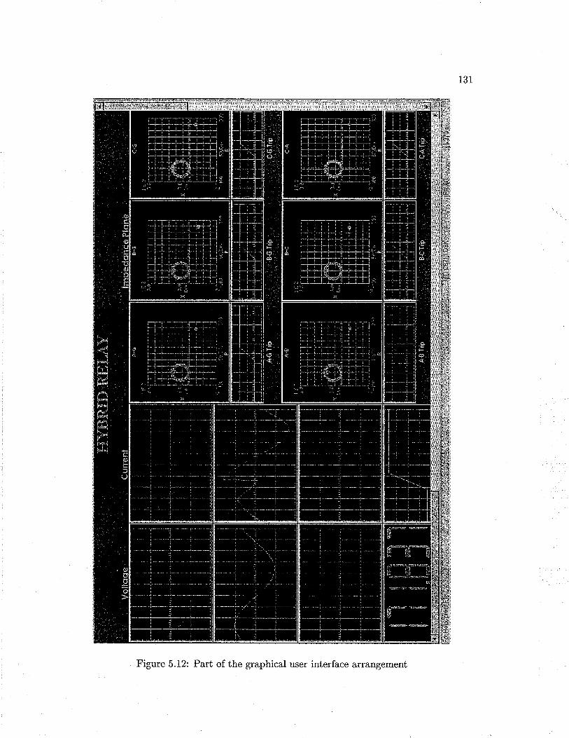
131
Figure 5.12: Part of the graphical user interface arrangement

r32
The hybrid relay algorithms processed the samples and issued a trip signal if a fault
condition within the protection zone was identified. The C6711 DSK does not have a
digital output channel. Hence the trip signal was "tapped" from one of the user outputs of
the C671i DSK. This signal was fed back to the RfP to record the trip signal and measure
the fault detection time. The user output signal of ihe DSK is a TTL output (5V). Höwever
the RTP required an input voltage of 20V or more to identify a digital input as "high". The
TTL output of the DSK was "amplified" using a peripheral drive array integrated circuit
Motorola MC1413 before connecting it back to the RjTP. The relay prototype and the test
setup are shown in Fig.5.13.
Figure 5.13: The setup used for testing the hybrid relay
Waveforms were generated for single-line.to-ground, line-line, and line'line.ground faults
using PSCAD/EMTDC. These waveforms were played back using the RIP and were used
for testing the relay. The RTP displays the trip signal along with the waveforms played
back and hence can be used to measure the trip time of the relay. The current and voltage
waveforms and the relay trip signals captured by the RTP for a three pha"se to ground fault
are shown in Fig.5.14. These waveforms correspond to a fault that occu¡red 325km away
from the relay location R. Out of the two irip signals shown, the bottom one corresponds
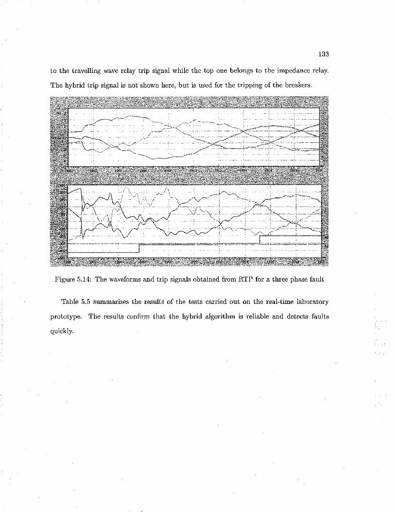
133
to the travelling wave relay trip signal while the top one belongs to the impedance relay.
The hybrid trip signal is not shown here, but is used for the tripping of the breakers.
Figure 5.14: The waveforms and trip signals obtained from RTP for a three phase fault
Table 5.5 summarizes the results of the tests carried oui on the real-time laboratory
prototype. The results confi.rm that the hybrid algorithm is reliable and detects faults
quickly.
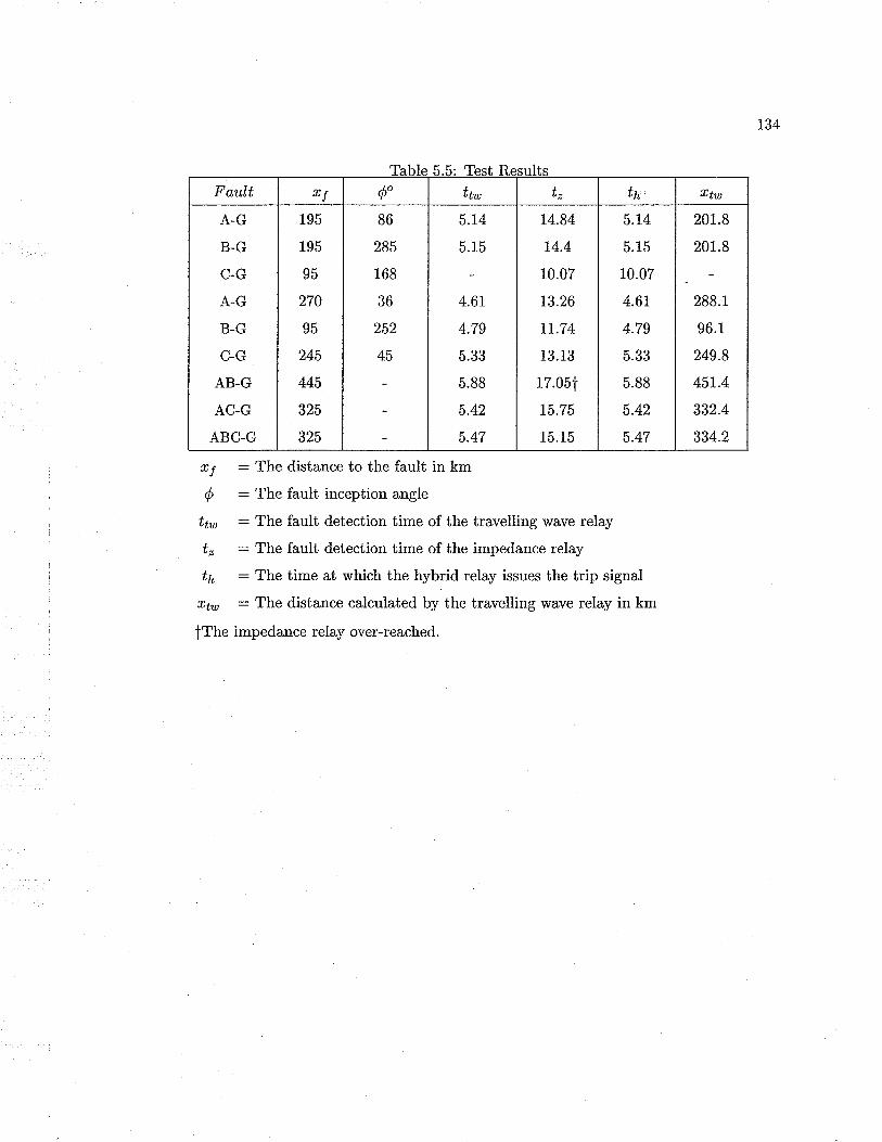
Fault rÍ óo ILtut t" tn rhu
A-G
B-G
C-G
A-G
B-G
C-G
AB-G
AC-G
ABC-G
195
195
95
270
95
245
445
325
325
86
285
168
36
252
45
5.L4
5.15
4.6r
4.79
É .).trJ. Ðd
5.88
5.42
5.47
74.84
14.4
10.07
L3.26
t7.74
13.13
17.05i
t5.75
15.15
5.L4
5.15
10.07
4.6r
4.79
5.33
5.88
5.42
5.47
201.8
201.8
288.1
96.1
249.8
45L.4
332.4
334.2
134
rf : The distance io the fault in km
ó : The fault inception angle
tn : The fault detection time of the travelling wave relay
tz : The fault detection time of the impedance relay
t¡ : The time at which the hybrid relay issues the trip signal
rtw : The distance calculated by the travelling wave relay in km
tThe impedance relay over-reached.
Chapter 6
Conclusions and Recommendations
Conclusions
The thesis examined how the measured impedance at the relay location and ihe fault
generated high frequency transient wavefronts can be combined in a single relay to find
solutions for the negative features associated with each method and improve both speed
and reliability of the protection scheme. Distance protection algorithms based on transient
signals provide a number of significant advantages but not without some limitations. The
travelling waves initiated by a fault depend not only on the fault position but also on the
fault type, the fault inception angle, fault impedance and the power system configuration.
These factors consequently have an infl.uence on the reliability of the decision made by a
travelling wave protection scheme. The ûrst wavefront initiated by a fault that appears
at the relay location contains information about the fault direction, fault type and fault
inception angle. This initial information can be used to determine whether the travelling
wave algorithm will be able to identifu a disturbance and classify it as an internal or external
fault. Internal and external fault classification is achieved by measuring the distance to the
fault. The distance is measured by observing the return of the initial forward wave to the
relaying station after being reflected at the fault location. Two main problem areas have
been identified with travelling wave protection: close-up faults and single phase faults that
135

136
occur near a voltage zero.
Distance protection schemes based on impedance measurement have shown their re-
Iiability over several decades. But the fault detection speed of impedance relays cannot
be further improved without compromising the reliability of the reach setting. However,
impedance relays are capable of detecting faults with small inception angles and the mea-
sured impedance quickly moves inside the protection zone for close-up faults. The hybrid
protection scheme proposed in this thesis takes advantage of these features so that the
impedance relay will detect the fault in case the travelling wave relay fails. The simulations
carried out on a simple 500kV three phase power system have shown that the hybrid relay
not only improves the speed of fault detection, but also maintains the reliability of the
overall scheme.
The ihesis also looked at how the zone 2 protection of a distance relay can be accelerated
without the aid of a teleprotection scheme. The proposed algorithm improves the reliability
of the travelling wave protection algorithm by combining the output of the zone 2 element
with the travelling wave distance calculation. Since the zone 2 element of the impedance
relay "monitors" the trip decision of the travelling wave relay, possible mal-operation of the
travelling wave relay due to switching transients is avoided. Since both algorithms check
for the presence of a fault, the inherent redundancy improves the reliability of the relay.
However for faults on the line which occur beyond the maximum allowable measurement
distance of the travelling wave scheme, a suitable inter-trip scheme will have to be utilized
to clear such faults in a timely fashion.
A laboratory prototype of the hybrid relay was implemented on Texas fnstruments
TMS320C6711 DSK. The voltage and current waveforms were obtained using ADS8364
EVM. The ADC is capable of providing samples at a high sampling rate while the DSK
performs the relaying functions of the two algorithms in real-time. The cost of the prototype
was kept as low as possible considering the needs of commercial production. The tests
carried out in the laboratory using generated waveforms showed the capability of the hybrid

137
relay prototype in detecting faults quickly with a high reliability.
Suggestions for Further Research
Further work is recommended as an extension of this thesis in the following areas:
1. The current and voltage at the relay point are measured with current transformers
and voltage transformers. In EHV lines, the voltage is usually measured using ca-
pacitive voltage transformers (CVT). All these transducers have a limited bandwidth,
especially the CVT which has a bandwidth of around 1000H2. Hence the measured
signals of the voltage waveform may not include the information of the high frequency
transients. This can reduce the relay algorithm's ability to detect faults using travel-
ling waves. However, the current transformers have a fairly high bandwidth of several
hundred kilohertz [B]. The measured waveforms of the current will contain most of the
high frequency transient components of the wavefront. The possibility of modifiiing
the travelling wave algorithm to detect faults only using current signals has to be
studied.
2. In the second algorithm of the hybrid relay, the zone 2 operation is used to monitor the
travelling wave relay. The travelling wave relay waits until the measured impedance
enters zonle 2 before issuing a trip signal. The speed of the hybrid relay can be further
improved by reducing this "wait time". Any movement of the measured impedance
towards the protection zone can be used as an indication for the presence of a fault.
Since the travelling wave relay already determines the location of the fault, the initial
movement of the impedance towards the protection zone may be used to trigger the
travelling wave trip signal. Since the travelling wave scheme is immune to power
swings or load variations, the reliability of the hybrid relay will still be high.
3. The proposed hybrid scheme was only simulated and tested on a simple three phase
power network. F\rrther tests have to be carried out to study the behaviour of the

138
4.
scheme in a complex po'trer system.
The hybrid relay was not tested on a system with series compensation. It is evi-
dent that series compensation will not cause a significant effect on travelling wave
relays because the reiay makes its decision before the operation of the series capacitor
protection circuit. The high frequency transient signals see the series capacitor as a
short circuit and hence will not be much affected. However, the re-insertion of capac-
itor compensation after an external fault may develop transient signals and requires
further study.
This thesis did not consider the fault impedance values higher than 25f). A high fault
resistance affects the reflected wave quantity and increases the transmitted component.
A detailed study has to be done how the results of the two algorithms can be effectively
combined to detect high impedance faults.
The fault which occurs at a fault inception angle near zero requires further investiga-
tion. A proper differentiation method of the relaying signals for such cases must be
developed to make correct identiûcation of such faults.
The hardware implementation requires further improvements in order to simptify the
relay functions, improve the speed and lower the cost. Also, the use of high bandwidth
field data instead of the off-line simulation data would be very helpful to permit the
study of the effect of noise.
5.
6.
t,

Appendix A
Transmission Line Theory
When the length of a transmission line increases, both potential and cur¡ent at any instant
may vary appreciably with the distance along the line. When the lines are too long, the
Iumped parameter models of transmission lines no longer would give valid results. In such
circumstances, distributed parameter model is used. This section will describe the behaviour
of voltage and current signals in long transmission lines.
Lossless Line
The propagation characteristics of signals on transmission lines can be determined by a
transient solution of the basic equations. First, an ideal lossless line which has no series
resistance and shunt admittance will be examined.
Characteristic Equations
Suppose that at some instant, voltage u and current 'i are distributed along a lossless
transmission line of inductance Z per unit length and capacitance C per unit length as
shown in Fig. 4.1. The distributions will be both functions of distance r and time ú. The
139

140
I(x,t) I(x+Lx,t)---->
V(x,t) V(x+Lx ,t)
(b)
Figure 4.1: The distributed parameter model of a transmission line (a) a section of unitIength(b) the transmission line
voltage and current distributions are given b¡
u :V(r,ú) and i,: I(r,t) (A.1)
Then the total capacitanceNow, consider two points on the line at distances r and r* Lr.
current over the section A¿ is
I(r,t) - I(, * Aø, ú) :
Now if Aø is made to tend to zero,
f+^r c.?.¿,J" öt
I#,I:."' c.fi.a, : n* c fiHence
,. I(*,t) - I(r * Ar, ú)rrlJ-.Az-+0 L,r
c.yöt,
nô,-\t.- öt
aiôr
(A.2)

r41
Similarl¡ the potential difference between the two points at distances ¿ and rr * Ar is
given by the inductive drop over the section A.r, i.e.
¡r*An ôiV(r,t) -V(* * Ln,t): J" L.ä.tu (4.3)
Using the same argument as above, it is possible to show that
aY: -t.* (A.4)ô" - "'at
Differentiating (4.2) with respect to time,
a2i n ôr,aù: -c. aF (A.5)
and differentiating (4.4) wiih respect to distance
ô2u _ , ô'iaæ - -"'arat
Flom (A..5) and (4.6),
(A.6)
(A.7)
and a similar elimination yields
(A.8)
Solution of the equation
The solution can be found in the same way for both wave equations (4.7) and (4.8). A
solution method was introduced by dAlembert for this type of equations. The wave equation
(A..7) is of the form
ô2u , ô2u
ôt, : o"' Ar, (A'9)
o2u -,no"ôr2 "-'Azt
a2i' - rnô'i
0x2 -"'Azt

r42
where a : Llt/ LC. (.{.9) is first transformed by introducing the new independent variables
r:r*at and s:t-at (A..10)
Then voltage u and current e become functions of r and s. Hence using the chain rule, Ieft
hand side of (A.a) can be expanded to give
0u ôu ôr ôu ôs ðu ðuj_- --_--+-- (A.11)ôr ôr'ôr ' ôs'ôr - ôr ' ðs
Squaring (,{.11),
Squaring (4.13)
Similarl¡
Substituting (A..12) and (4.i4) in (A'.9),
ô2uã:ã: :0 (A..15)Ords
Now, (4.15) can be solved with two successive integrations. Integrating with respect to r
H:.þ) (A.16)
where tø(s) is an arbitrary function of s, independent of r. Integrating with respect to s
ô'r:0'u *rô', -ð',ôr2 ôr2 '-ôrôs' 0s2
ôu ôu ôr ôu ðs lôu âu\at: ar'at* æ'æ:"(* - a")
ô2u n/ô2u -ô2u ô2u\at,
: o" \ur, -
2 ôras
* up )
't) : I' wþ)as + fzî): f1(s) + fz(r)
(A.12)
(A.13)
(4.14)
(A.17)
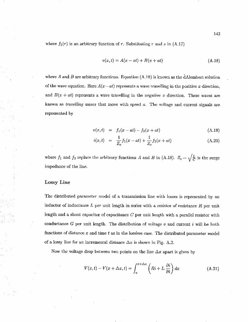
t43
where /2(r) is an arbitrary function of r. Substituting r and s in (,{.17)
u(r,t) : A(r - at) * B(r + at) (.4..18)
where ,4 and B are arbitrary functions. Equation (4.13) is known as the dAlembert solution
of the wave equation. Here A(x - at) represents a wave travelling in the positive z direction,
and B(r * aú) represents a wave travelling in the negative r direction. These waves are
known as trauelling uaues that move with speed a. The voltage and current signals are
represented by
u(r,t)
i,(r,t)
ft@-at)-f2(r+at)
Lr'o-at)+lÍ,@+ot)
(A.1e)
(A.20)
where fi and /2 replace the arbitrary functions Á and B in (4.18). z": ,Q "the surge
impedance of the line.
Lossy Line
The distributed parameter model of a transmission line with losses is represented by an
inductor of inductance -L per unit length in series with a resistor of resistance .l? per unit
length and a shunt capacitor of capacitance C per unit length with a parallel resistor with
conductance G per unii length. The distribution of voltage u and current ,i will be both
functions of distance r and time ú as in the lossless case. The distributed parameter model
of a lossy line for an incremental distance Ar is shown in Fig. 4.2.
Now the voltage drop between two points on the line Ar apart is given by
v(r,t) -V(** ar, ù : I, " (*n + t .fi) n (A.21)
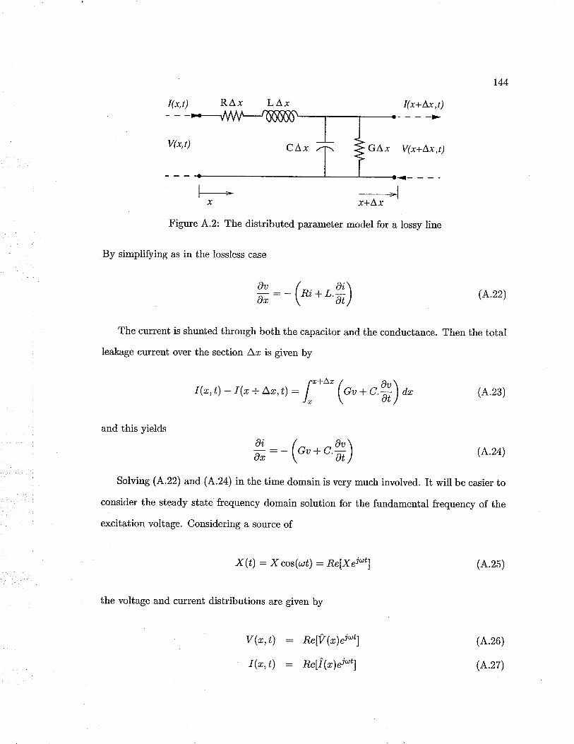
I(x,r) RÁx L A,x I(x+Lx,t)
V(x,t)
r---.---.-x
Figure 4.2: The distributed parameter model for a lossy line
By simplifuing as in the lossless case
X:-(''*'i')
------=lx+A.x
The current is shunted through both the capacitor and the conductance. Then the total
leakage current over the section Ar is given by
and this yields
I(r,t) - I(, i Lr,Ð : l, " ("' + c.fi) a"
#:-("'* "X)
r44
(L.22)
(4.23)
(A.26)
(^.27)
(4.24)
Solving (A'.22) and (4.24) in the time domain is very much involved. It will be easier to
consider the steady state frequency domain solution for the fundamental frequency of the
excitation voltage. Conside¡ing a source of
X(t): Xcos(øú) : ReïXei"tl
the voltage and current distributions are given by
(A.25)
V(n,t): Ae[Vçr¡d'tl
I(r,t) : nelÎ@)d'tl

ôu
a*: - (R+ jwL).i,
and
dr,
or: - (G + ¡wc) .u
Difierentiaiing (4.28) and substituting from (4.29) lead to
#: (R+ jaL) (G + juc) .u
Considering only the real part of the voltage and current
and
a2iaa : (Ã + jaL) (G + jwc) .i
I45
(A.28)
(A..2e)
(A.30)
(4.31)
(A..34)
(A.35)
(A.32)
(A.33)
'Y2u
t."y'2
. v+ _-_ v-'ia: -¿-1r
- '-
e'wLc Lî.
Thecoefficient@isknownaspIopagationconstant,7.Then
ô2u
aæ:ô2iA"'z
:
The solution for (A..32) and (4.33) is given by
ur : Vte-1' +V- e't'
and
where
(R+ jaL)(G + juc) (A.36)

Appendix B
Three Phase Transmission Lines
Derivation of 3-Phase Tbansmission Line Equations
Equivalent Circuit
A 3-phase transmission line composed of three conductors parallel to the ground is shown
in Fig. 8.1. The sending end is considered as the generating point while the receiving end
normally consists of a load, The voltage and current signals will be functions of position
c along the line usually measured from the sending end and time ú measured from some
reference time.
The equivalent circuit approximation of a difierential length of the transmission line
Vo(x,t) Vâ(L,t)Ia(x,0 LG.ù
vb(0,0 vb(L,0Il0,r)
SENDING LIb(L,Ð
--¡. RECEIVING
va(0,r)
t(0,0
Vb(x,0lb(x,t)
END END
vc(L,ÐI"(L,0
vc(0,0
*O _-* x=L
Figure 8.1: Representation of a three phase transmission line with an earth return
L46
V"(x,Ð
L(x,t)
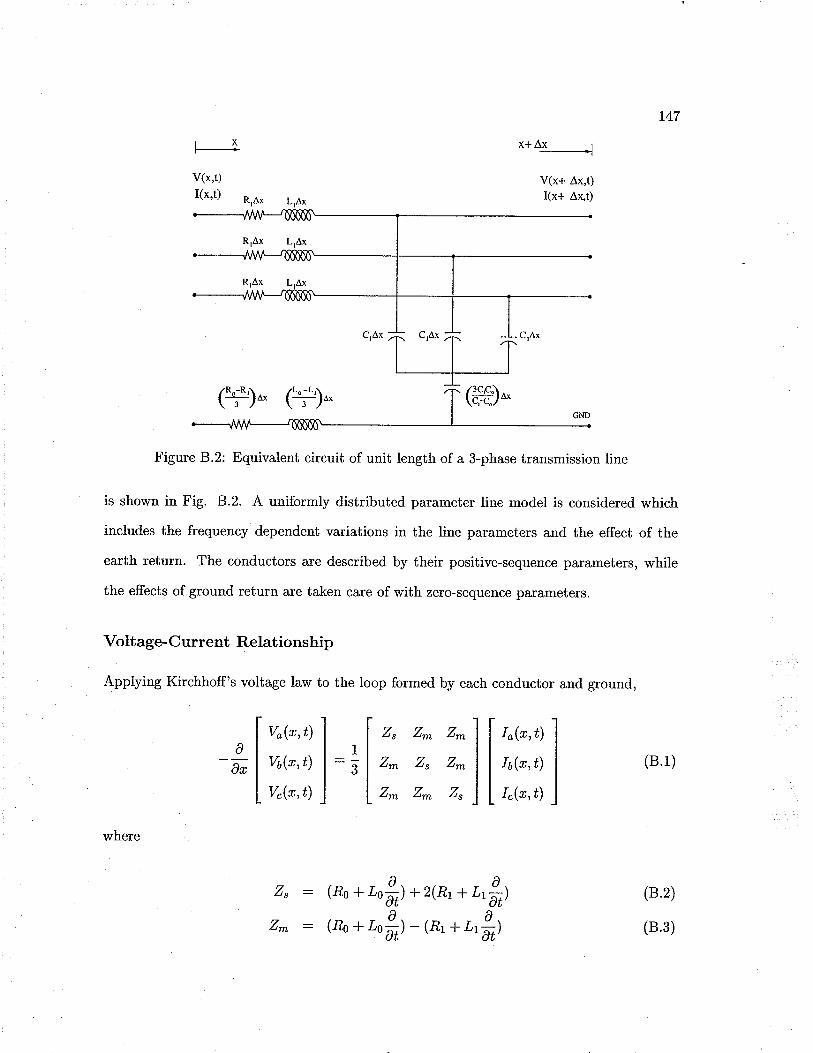
rx
V(x,t)I(x,t)
R,Áx
I"(r,t)
I6@,t)
I"(r,t)
r47
(8.1)
x+Âx r-----------t
V(x+ Ax,t)I(x+ Ânt)L,Áx
Figure 8.2: Equivalent circuit of unit length of a 3-phase transmission line
is shown in Fig. 8.2. A uniformly distributed parameter line model is considered which
includes the freguency dependent variations in the line parameters and the effect of the
earth return. The conductors are described by their positive-sequence parameters, while
the effects of ground return a¡e taken care of with zero-sequence parameters.
Voltage- Current Relationship
Applying Kirchhoff's voltage law to the loop formed by each conductor and ground,
where
ïllr"@,r)1 | z,
-*l vbþ,tt) l:Il '*lnø,,) I I '*
(8.2)
(8.3)
zs:17zJ 7¡¿
zm
z"
z^
(Ão+ tr*l+z(RL+Lr*)
(Æo + u*r)- (Er + Lr*)
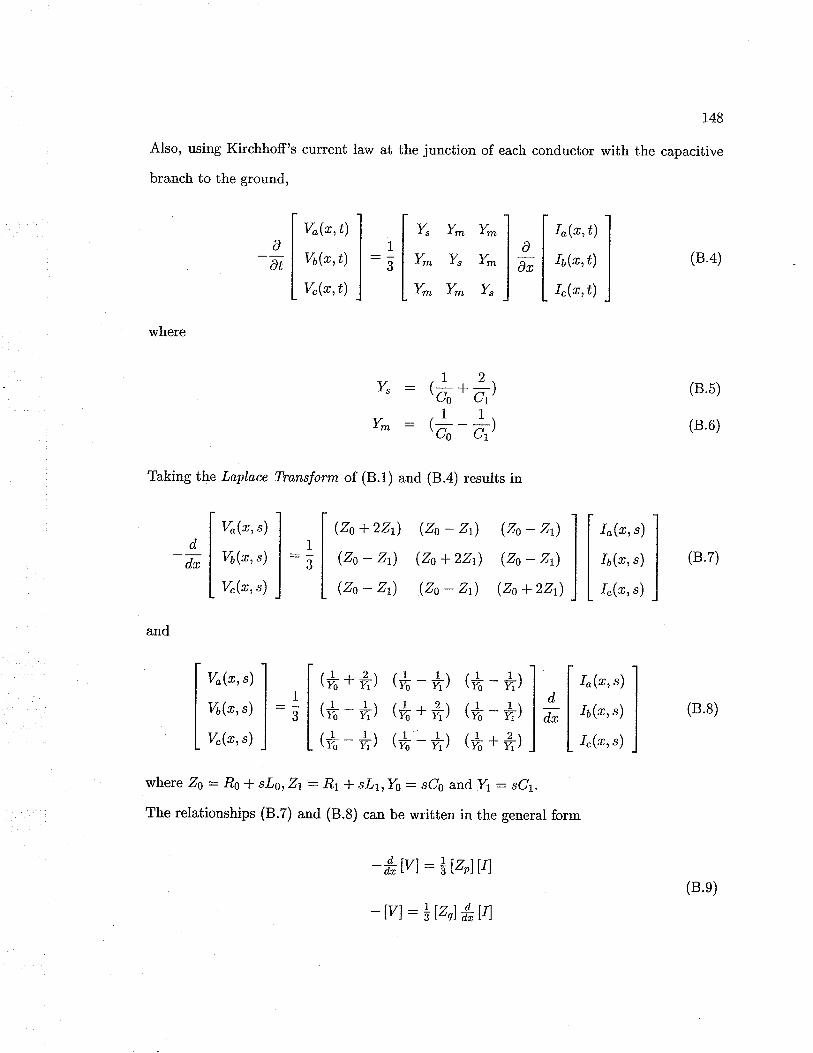
r48
Also, using Kirchhoff's current law at the junction of each conductor with the capacitive
branch to the ground,
ðA"
I t, Y* Y,n1l:slv* Ys Y*
Lt* Y* Y,
a-at
V"(r,t)
V6(r,t)
V.(r,t)
Io(x,t)
16@,t)
I.@,t)
(8.4)
(8.5)
(8.6)
(8.7)
(8.8)
where
Taking the Laplace Thansform of (8.1) and (8.4) results in
Y" : 'ä.
ä'Yrr : ,ä- ä,
(zo + 22ù (Zo - Zt) (Zo - Zù
(Zo - Zt) (Zo + zZt) (Zo - Zt)
(zo - zù (zo - zt) (zo + 22ù
++) (+-+)- #) {f,, + fr,)
-+) (+,-+)
1
.)*lW(r,s)
v6@,s)
V.(x, t)
I"(r, s)
I6(x, s)
I.(r, s)
and
Vo(x, s)
V6(r, s)
V.(*, ")
(+-+) I
(+++) l
ir+:ål (+.
L,+
Io(r, s)
16(r, s)
I.(r,, s)
where Zo : Rn I sLs, Zt : Rt * sLlrYo : sCo and Y1 : sCr.
The relationships (8.7) and (8.8) can be written in the general form
-*tvl: llzoll4
- ïvl : IlzÀ *trl(B.e)

I49
Solution to the equations
By eliminating the current matrix [1] of (8.9), a second order differential equation involving
the voltage matrix can be obtained.
where
The equation (8.10) does not have a simple solution because the coefficient matrix [p] is
not diagonal. Using a transformation of variables, the actual voltages V canbe transformed
to another set of components [/.
firrl- [r,][v] : o
lvl: lrl[ullul : ["]-1Ml
where ["] is the transformation matrix. Now (8.10) can be written as
fivl-[z][u] :s
| {to"o +2zLyt) (zoyo - zfù (zoyo - ztyt) ltøl : | | Øoto- ztyt) (zoyo+zzLyt) (zoyo- zÍt) | tu.ttl
| Øo"o - ztyt) (zoyo - zÍù (zoyo + 2zÍt) l
(8.10)
(8.12)
(8.13)
where
[r] : ["]-r i¡rltrl (8.14)
With a proper choice of [7], it is possible to make [r] diagonal. Now (8.1J) can be
readily solved since it is a set ofan ordinary second-order differential equations with constant
coefficients.

150
With proper transformation, the transmission line components of (8.11) become,
[,] : ["]-1 U"l[r]:
ZoYo 0 0
0 Z1Y1 0
0 0 ZtYt
[u(t¡1 : [,9][u{-)1t¡1
[i(¿)] : [8][¿(r¿)(¿)]
(8.15)
(8.16)
Hence, the three-phase system is now represented with three independent systems 6¡
modes. This method is known as modal transformation.
Modal Tbansformation
Basic Principles
A line consisting of n conductors and ground has r¿ modes of propagation. Each mode has
a particular voltage-current relationship, velocity and attenuation constant at any given
frequency. To analyze the transient behaviour of a 3-phase system, the voltages and cur-
rents are converted into modal quantities. The modal transformation techniques convert a
dependent n-line system to n independent modes.
A transformation matrix as in (8.15) is used to find the modal quantities. The trans-
formation of voltage and current signal use two transformation matrices. (8.16) shows the
relationship between phase and modal quantities.
where [,9] and [8] *" the voltage and current modal transformation matrices respectively.
¡u{-)1t¡1 and [Z(-)(t¡] are the modalvoltage and current mat¡ices. The inverse relationship
is given by (8.17).
¡u(-) 1r;1 : [S]-t [?,(ú)]
[i(,n) (ú)] : [g]-1 [i(ú)]
(8.17)

151
The relationship between voltage and current of an n line system is given by (8.18) and
(8.1e).
davl :drd,lr) :dx
-øta+
-tRt-vl
: -azrLer7(*)l
: -[,s]-t azlwl7(^)l
: -¡Z{^)¡7{*)1
(8.18)
(8.1e)
(8.20)
where the matrices have the dimensions corresponding to the number of modes. Applying
modal voltage quantities to (8.18) yields
fiuatv'*'ltfiuv'^'lt
where [Y(-)] : tçl-tl-yl[^s].
Modal Tlansformation Matrices
The modal transformation matrices [,S]and
of propagation. The most commonly used
Wedepohl transformations.
where ø@l: [S]-'aZ)lQl. Similarly from (8.19), it is possible ro show rhar
ftff'*' lt : - ¡r(-)1 ¡y(-)1 (8.21)
[Q] can be chosen to give independent modes
transformations are Karrenbauer, Clarke and
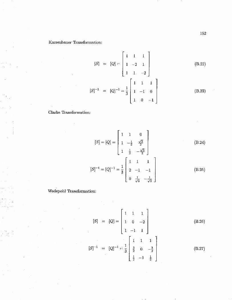
752
(8.22)
(8.23)
(8.24)
(8.25)
(8.26)
Karrenbauer Transformation:
ll t:i
l
,it I 1l:511 -1 o
I
L' o -'j
l-,, o_l
l'-++lf r + -+l
:åi"),-" 1lo h -#
1
-112
ll I ):
:+ll:,
Clarke Tbansformation :
lsl : l8l:
[.9]-t : [g]-'
[s] : [g] :
[s]-' : [g]-'
tsl : LQ):
[g]-'
Wedep ohl Tlansformation:
(8.27)[,s]-t :

i53
The modal quantities evaluated will have 3 modes, two aerial modes and an earth mode.
c Earth mode lMode Ll
This is the zero sequence component of the phase voltages and currents. Its velocity and at-
tenuation will be affected by the resistivity of the earth and hence it is frequency dependent.
Velocity at low frequencies may be approximately 75% of the speed of light.
¡ Aeri,al modes [Modes 2 and 3]
In these modes, the current in the 3 phases tend io cancel. Therefore the effect of ea¡th resis-
tivity in that mode is very small. Hence the aerial modes are almost frequency independent
and the velocities approach the speed of light.
Modal Impedance and Velocity
For a three phase system
avl:a*)l¡r (8.28)
where Zf)i" the phase characteristic impedance matrix. Using modal transformation, we
get
v@)l : rsl-' tz?nelT(*)l
-/-\ -¡l-\fzi''1¡¡v''t7
where Z!)i"the modal characteristic impedance matrix.
For a fully transposed line section (symmeirical configuration), @!)] is diagonal.
(8.2e)
0 0lZtrl, ,r)
Itor*'l:l o
L,(8.30)
154
where Zs is the impedance of the earth mode and 21 and 22 are the impedances of the
aerial modes. In (8.30)
Zs : Zssi2Zsrn
21 : Zz: ZoS - Zo*
where
Zo" : self impedance term of phase characteristic impedance matrix
Z0* : mutual impedance term of phase characteristic impedance matrix
The two aerial modes and the earth mode have different velocities. The earth mode
velocity depends on the ground impedance. The aerial mode velocities are almost indepen-
dent of the ground resistivity hence frequency, and are close to the speed of light. Mode 3
velocity is usually slightly higher than that of Mode 2.

Appendix C
Signal Processing Techniques
Different signal processing techniques a¡e used in practice to detect required signals from
the measured waveforms under noisy conditions. The most commonly used technique in
detecting wavefront reflections in travelling wave based protection schemes is the correlation
method. The theory behind the correlation function and its applicability to detect faults
under noisy conditions are described in this section.
Correlation in Analog Domain
The cross-correlation function of two time invariant signals ø(ú) and E(t) is given by
R*r(,): lim : f rþ).y(t * r)dtT-+æ'1' Jg
The covariance function of two signals ø(ú) and y(t) is
e,s(,): ;i5 L, lr' WfO - ¡l.laþ + r) - sldt (c.2)
where the mean values of the signals ø(ú) and g(ú) during the time period T are given by
(c.1)
1
155
u: I fo' *{')* r: + lo' ,{r)0, (c.3)

156
and þ(ú) - ¡1, [y(t) - g] give the deviation of the signal from the mean value within the
period concerned. Now expanding C.2,
1 f't: ¡r ¡TQ"s(r) : J*",t¿ x(t).y(t + r)dt -u. Jo a(t + r) -9. J, r(t)dt +î.9\
: ,t5"-+ for
r(t).u(t+r)dt-ã.;* + I,' s(t+r)-r ;iL + I,' r(t)d,t+î.r
: -li- I fr *ft).y(t * r)dt - r.T -î.a + r.ar'-+æT Js
: ü-1¡Ti'--ar Jo t(t)'s(t * r)dt -î'g
: R"y(") -r.T (c.4)
Tf g(t) is time variant,
e,s(') : ,H.å fr'ff-O -¡).1aft*") - + Ir'y(t+r)¿tl\¿t
+ l,' r(t)ú.+ I,' ,u + r)dt * r.# I l,' ,n + r)dtdt\
trT: ;X" J, r(t)'v(t + r)dt -z'aî) --r'u7) +r'v(r)
: ,t51 å lor
r(t).uft + r)dt -n.ffi: R*oG) -ø.ffi (c.5)
Correlation in the Digital Domain
In the digital domain the continuous variable ú is replaced with the sample number k.
The signals are sampled at a frequency at least twice higher than the maximum frequency
concerned. The autocorrelation function of a sampled signal c(k) is given by
1NR*(mLt):;t x(k\t).r(k\t+nx\t) (C.6)
lc=L

r57
where rn is the number of samples the two waveforms are shifted by each other. Here, Aú
is the sampling interval and N is the total number of samples in the time interval ?.
The cross-correlation function of the two signals z(k) and g(k) is given by
rNR,o(ma;t):;Ð n(k\t)g(k\t+rn\t) (C.T)fr:1
The covariance function of two signals with the mean removal is given by
1NQ,r(m\t): * It"(kat) -nl.fy(kat + m\t) _v?nat)l (c.s)
k=l
where
r : *Ë r@Lt) (c.e)k=L
1N!(m\t) : ;Is(kat*m\t) (c.10)
/c=1
Expanding the relationship given by (C.8),
rN@,r(m\t) : , Ðt"t*ot).y(ktt*mlt) -r.y(kLt+m\;) -
k=Lg (m 4;) lk At) + a.! (m Lt)j
lNrN: f f nftLt).y(k\t + rnat)- ã.; Ða?'tt + m\t)&:1 -' fr=1
-s{nznr).f Ë"1*o,1 + rg(mvtl} Ëttlk=! - ¡k:l
rN: n Ð r@Lt).y(kat + rn\t) _î.!(m\t) -g(m\t).r +r.!(m\t)lc=l
--¿V
* f x(k\t).y(k\t + rnht) -n.!(m/\t)¡k=1
R"u(m\t) -î.!(m\t) (C.rr)
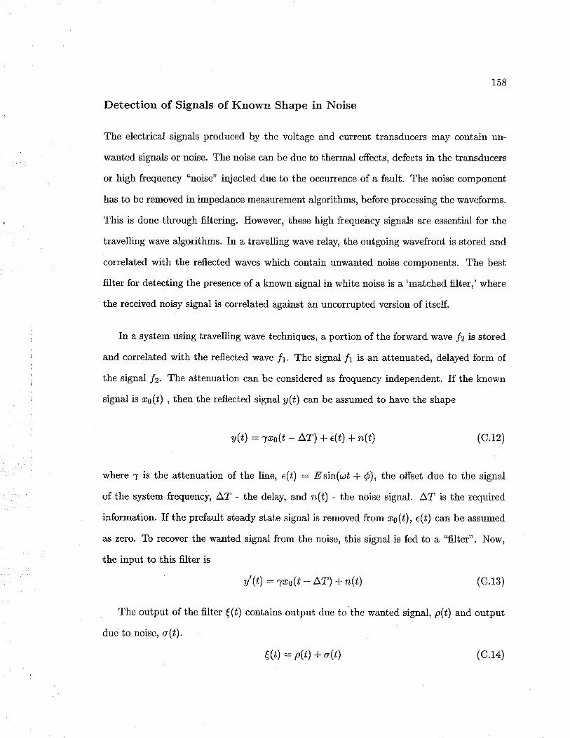
158
Detection of Signals of Known Shape in Noise
The electrical signals produced by the voltage and current transducers may contain un-
wanted signals or noise. The noise can be due to thermal efiects, defects in the transducers
or high frequency "noise" injected due to the occurrence of a fault. The noise component
has to be removed in impedance measurement algorithms, before processing the waveforms.
This is done through ûltering. However, these high frequency signals are essential for the
travelling wave algorithms. In a t¡avelling wave relag the outgoing wavefront is stored and
correlated with the reflected r¡/aves which contain unwanted noise components. The best
filter for detecting the presence of a known signal in white noise is a 'matched filter,' where
the received noisy signal is correlated against an uncorrupted version of itself.
In a system using travelling wave techniques, a portion of the forward wave f2 is stored
and correlated with the reflected wave /1. The signal /1 is an attenuated, delayed form of
the signal fz. The attenuation can be considered as frequency independent. If the known
signal is zs(t) , then the reflected signal y(t) can be assumed to have the shape
a(t) : tro(t - A") + e(t) + n(t) (c.12)
where 7 is the attenuation of the line, e(ú) : Esin(ut + /), the offset due to the signal
of the system frequenc¡ AZ - ihe delay and n(ú) - the noise signal. AT is the required
information. If the prefault steady state signal is removed from øe(ú), e(ú) can be assumed
a.s zero. To recover the wanted signal from the noise, this signal is fed to a "filter". Nov/,
the input to this filter is
y'(t):wo(t- AT)+n(t) (c.13)
The output of the filter {(ú) contains output due to the wanted signal, p(ú) and output
due to noise, o(ú).
{(¿) : p(t)+o(t) (c.14)
159
If the delayed signal of øs(ú) is given by ø(t),
r(t):ws(t-LT)
Consider the frequency spectrum of r(t).
X(u) :1Xs(u)¿-i'^r
where
(c.15)
(c.16)
(c.1e)
(c.20)
(c.17)
If the frequency response of the filter is H(r), then the required signal at the output of the
filter is given by
xo(ù: I:rs(t)e-i'tdt
p(t) : * I:H (u).xs(u)d,, d.
: + Ir' n21t¡ at
: +" I:sn(u)ù':
(c.18)
If the power spectral density of the noise signal n(t) is given by S"(r), then the average
power of ihe noise signal is
At the output of the filter, the total power of the noise signal N is given by
N : lo(ú)12 : * l:ln@)l' .s*(u)d.u:
Now, it is required to maximize the signal to noise ratio ¡1, at the output of the filter at
some instant in time, say ú: T. i.e.
,, - pz(r) -Þlå¡¡(')'xo tq"t'j{t":'-ñ-:ffi (c.21)

160
The maximization of the expression can be accomplished by applying the Schwartz i.nequal-
itv
la /* p(w).e.@7"i"a,1' = f p@)12d.. [* @@)l'd- (c.22)
lz" J _* I J_oo J_oo
where Q* is the complex conjugate of Q. The equality applies when P : constl,ntxQ.
Therefore,
/å l¡¡tr) l' ¿r. [ï* lxs(u)12 du
* [:*lH(,)l' .s^(a)dnt
H(u): O"-i'rI@
The optimurn fiIter is a fiIter that maximizes ¡,t, i.e. the optimum filter is obtained at t : T,
when
(c.23)
where K is a constant. The frequency response is proportional io X¡(ø) which emphasizes
frequencies which contain large signal components and inversely proportional to S"(r) which
de-emphasizes frequencies which contain Iarge noise components. If the noise is considered
tobe ad,d,itiue whi,te noise, LE.l,9r(ø)12:1, then the optimum filter is the matched, fiIter
or correlator. The transfer function of the correlator is given by
H(u) : e-i'r Xö(r) (c.24)
Then in the time domain, when X6(ø) is real, i.e. when the input signal u (ú) is symmetrical,
h(t) : Kr(t -r) (c.25)
That is, the impulse response of the filter is matched to the delayed replica of the input
signal to which ihe filter is matched. Hence the correlation technique becomes an effective
method to extract a known signal in white gaussian noise.
Appendix D
Impedance Measurement of
Transmission Lines
Introduction
The basic principle behind impedance relaying is calculating the line impedance seen by
the relay at the relay location using the fundamental frequency components of voltage and
current signals. The impedance is a function of the voltage and current. Fourier transform
based methods can be used to derive the fundamental components of the voltage and current
signals. In this section, the basic theory behind the impedance measurement algorithm is
introduced.
Impedance Calculation
Fourier analysis can be used to calculate the fundamental frequency component. According
to the definition of Fourier Series, in the analog domain, a signal ø(ú) which repeats with
period T canbe expressed as a sum of cosines and sines as
n(t):oo+ I ancos(nuçt)+ I bnsin(nttst) (D.1)n:l n=l
161

r62
where
an:
bn:
O,O
I1,,
t t,'+ 1,,
r(t) cos(nu6t) dt
ø(ú) sin(na.'st) d,t
r(t) dt (D.2)
and as represents the dc component. Here, uo : 2tr lT. The Fourier analysis separates the
dc, fundamental and harmonic components of /(ú). For the ntô harmonic, the amplitude is
given by
lc.l: t/@Tñ (D.3)
and the phase angle is given by
(D.4)
The fundamental frequency components are given by ø1 and ô1.
The Fourier series has certain practical limitations in its use. It assumes that the time
function is of infinite duration, whereas practical data in the case of a fault are often
a transient having finite duration. Further, it assumes that the data are periodic over an
unlimited extent, whereas practical data are usually non-periodic. It is possible to represent
non-periodic daia by a Fourier Tbansform (FT). The FT of the time function ø(f) is given
by
,,n:tan-L (*)
x(f): I* "n e-iuto, (D.5)
where u:ZtrlT. The absolute value of (D.5) yields the frequency amplitude content and
the argument gives the phase content.
In digital algorithms, sampled values are used instead of the continuous variables. Hence
the continuous integrals given by (D.2) cannot be applied directly to find the fundamental
components. Instead the integral is taken over -l{ samples within the time interval ? which
163
immediately precedes the sampling instant in question. The digital domain equivalent of
(D.1) is given by,
(N -t) /2 / ^ \ (N- 1)/2
r(k):oo*' Ðu
Ancos(T*)+'i' Bnsin(T*) (D.6)
where n : 0,L,2,.......,(N - L)12 and ,k : !,2,........(¡f - 1). The discrete form of the
integrals are given by
where u(k) represents individual samples within the sampling window. This is known as
the discrete Fourier series. The amplitude and the phase of the nÚh harmonic is given by,
lC,l:\/@;ø
and
on:tan-r (X)The fundamental frequency components are given by Al and By
The discreie form of (D.5) is given by
An: #tÐ'ø(k)cos (T*)k=0
Bn: #'Ð'ø(k)sin (T*)fr=0
A6: *tÏ'",*,/c:0
. (N-1)x(n): + I x(k)e-t(T"n)
IYk=0
(D.7)
(D.8)
(D.e)
(D.10)
where lí,n : I,2,..........N. The above relationship is known as the DFT. A major use
of the DFT is the translation of a time series into an equivalent frequency series. Hence

164
the DFT can be used effectively to calculate the fundamental components of voltage and
current signals. An alternative method of obtaining the DFT, termed as the FFT, can be
used to improve the speed of calculation when a number of DFT's are sought (e.g. the
fundamental and several harmonics).
Using (D.8) and (D.9), the fundamental components of the voltage and current can be
obtained.
(D.11)
and
ot:tan-t (fr) (D.12)
Using the above equation, the voltage Cv, 0v and current Ct,0t fundamental phasor
components can be obtained. The imped anceZ and phase angle 0 s can be derived by using
lzl : CvC,
ov-ot
(D.13)
(D.14)02:
The above computation is carried out at each sampling interval. This will give an
impedance value based on the voltage and current samples of the previous cycle preceding
the current sample.
In a three phase system, the mutual coupling between transmission lines affects the
sound phases when there is a fault on one phase. If the voltage and current signals from
each phase are used to find the impedance according to the above method, the impedance
value obtained will not be proportional to the distance to the fault. Thansforming phase
variables to symmetrical component variables avoids mutual effects between variables except
at the fault location.
(A?+ B?)

165
Symmetrical components
If a fault occurs in a three phase network, the mutual impedance between the phases allows
fault induced effects to couple across from the faulted phase to the sound phases.If the
impedance is calculated from the line voltages V6,V6,V. and currents I,,16,I" of the three
phases, the calculated values will not have a simple relationship to the distance to the fault.
To decouple the phases, the three phase network can be transformed into a new set of
phasors known as symmetrical components. The new set of components a¡e labelled the
012 set. They are referred to as the zero sequence, positive sequence and negative sequence
components [108].
The three phase system can be expressed in a concise form as in (D.15),
[V"u"] : [Z"u"]lI"u"l (D.15)
where Vou.is the voltage vector, Io6"is the current vector and Zo6" is the impedance matrix
of ihe network. The matrix 2o6" lr;as mutual elements. This can be transformed into a new
set of variables:
lVonl: lZon)llonl
The elements in (D.16) are related to the values in (D.15) bV,
(D.16)
(D.17)
lv"u"l
lI"u"l
ïFl-rlZ,b"l[F]
lrllYorzl
lFl[10'z]
[zon]
111lao,2
la2o,
1:*.)ll l':
where
lFl : lFl-' (D.18)

166
Here,
(D.1e)
The matrix Z6p in (D.17) is diagonal and the diagonal elements are the eigenvalues of
the 2o6" matrix if the system is assumed to be perfectly balanced. The diagonal elements
20, Zt, and 22 are known as zero, positive, and negative sequence impedance, respectively.
Mho Relay
The mho type distance relay is most suited for protecting long transmission lines. The mho
relay has inherent directional discrimination properties. The concept of the mho relay can
be explained using the universal relay torque equation [109] given as follows:
T : KtI2 * KzV2 * KyVI cos(O - r) + K (D.20)
where 0 is the angle between l and V, r the maximum torque angle, 1{ is the fixed restraining
torque and ,r(1 , Kz,KS are constants.
In the mho relay, the operating torque is obtained by the V-I element and the restraining
torque is due to the voltage element. Hence in D.20, K1 is set to zero. Neglecting K, the
torque equation becomes
T : KsVI cos(0 - r) - K2V2 (D.21)
For the relay to operate
KsVI cos(0 - r) > KzVz (D.22)
": (-;. t+) : Ltrzo, u : (-i-'+) : rt24o
z.Tcos(e-r) (D.23)
This characteristic when drawn on an impedance plane depicts a circle passing through the
origin. The relay operates when the impedance seen by the relay falls within this circle.

Appendix E
Line Configuration and Parameters
The transmission line configuration and parameters of the three phase power network used
for simulations in Chapter 4 are given here. The line parameters were generated by the
"Iine constants" program in PSCAD. The transmission line is assumed to have uniform sag
and conductor spacing along the total span. The tower configuration is shown in Fig. E.1.
o,1 ----jts- ---'' Gz
Çc,h"i I
"t tri i""cro ú i.---x-^----oc¡
I"c
i
I
I
inrc
Figure E.L: Tower configuration
r67
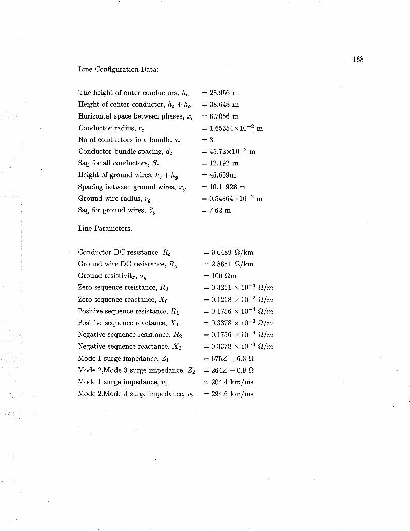
168
Line Configuration Data:
The height of outer conductors, å."
Height of center conductor, h" + ho
Horizontal space between phases, z"
Conductor radius, r"No of conductors in a bundle, n
Conductor bundle spacing, d"
Sag for all conductors, ^9"
Height of ground wires, hc+ hs
Spacing between ground wires, ø,
Ground wire radius, r,Sag for ground wires, ,Sn
Line Parameters:
Conductor DC resistance, R"
Ground wire DC resistance, -R,
Ground resistivit¡ o,Zero sequence resistance, R4
Zero sequence reactance, X6
Positive sequence resistance, .R1
Positive sequence reactance, X1
Negative sequence resistance, .R2
Negative sequence reactance, X2
Mode 1 surge impedance, 21
Mode 2,Mode 3 surge impedance,
Mode 1 surge impedance, u1
Mode 2,Mode 3 surge impedance,
: 28.956 m
: 38.648 m
: 6.7056 m
: 1.65354x10⁻² m
:J
:45.72xL0-2 m
:12.192 m:45.659m
: 10.11928 m
: 0.54864x10⁻² m
-- 7.62 m
: 0.0489 A/km: 2.8651 C)/km
: 100 f)m: 0.3211 x L0-3 Qf rn
: 0.1218 x L0-2 Qf rn
: 0.1756 x t0-4 Qlm: 0.3378 x L0-3 Qf rn
: 0.1756 x I0-4 Qf m
: 0.3378 x t0-3 Qlm:6751= 6.3 O
:2641- 0.9 Q
:204.4 km/ms
:294.6 km/ms
Z2
U2

Appendix F
Hardware Information
Multichannel Buffered Serial Port
The multichannel buffered serial port (McBSP) consists of a data path and a control path,
which connect to external devices. Data is communicated to these external devices via
separate pins for transmission and reception. Control information (clocking and frame
synchronizaiion) is communicated via four other pins. The device communicates to the
McBSP via 32-bit-wide control registers accessible via the internal peripheral bus. The
McBSP block diagram is shown in Fig.F.11.
The main functional units of the McBSP are described below:
Tlansmitter The transmitter section is responsible for the serial transmission of data that
is written in DXR. The contents of DXR are copied to the transmit shift register XSR.
The transfer starts as soon as the transmit frame sync (FSX) is detected. One bit of
data is transmitted or shifted out of XSR on every transmit clock CLKX. New data
can be written to DXR using either the CPU or the DMA.
Receiver The data received on the DR pin is shifted into the Receive Shift Register (RSR)
on every receive clock (CLKR). Again, the actual shifting in of data begins afterlObtained from [78]
169

t70
Figure F.1: The McBSP block diagram
detection of a receive frame sync (FSR). The data in RSR is copied to a Receive
Buffer Register (RBR) and then to the Data Receive Register (DRR). The DRR can
be read by either the CPU or the DMA.
Sample Rate Generator This module generates control signals such as the transmit/receive
clocks and frame sync signals necessary for data transfer to and from the McBSP.
Clock generation circuitry allows the user to choose either the CPU clock or an exter-
nal source via CLKS to generate CLKR/X. Fhame sync signal properties such as frame
period and frame width are also programmable. FSR/X, CLKR/X are bidirectional
pins, and therefore can be inputs or outputs.
Events/Interrupt Generation The McBSP generates sync events to the DMA to indi-
cate that data is ready in DRR or that DXR is ready for new data. They are ¡ead
sync event REVT, and write sync event XEVT. Simitarly the CPU can read/write to
the McBSP based on interrupts (RINT and XINT) generated by the McBSP.
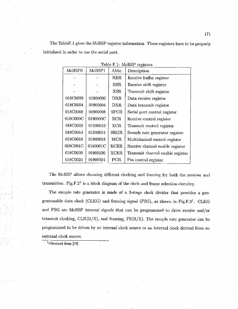
17L
The TableF.l gives the McBSP register information. These registers have to be properly
initialized in order to use the serial port.
Table F.1: McBSP.t:
McBSPO McBSPI Abbr. Description
018C0000
018C0004
018C0008
018C000c
018C0010
018C0014
018C0018
018C001c
0i8c0020
018C0024
01900000
01900004
01900008
0190000c
01900010
01900014
01900018
0190001c
01900020
0i900024
RBR
RSR
XSR
DRR
DXR
SPCR
RCR
XCR
SRGR
MCR
RCER
XCER
PCR
Receive buffer register
Receive shift register
Tlansmit shift register
Data receive register
Data transmit register
Serial port control register
Receive control register
T[ansmit control register
Sample rate generator register
Multichannel control register
Receive channel enable register
Thansmit channel enable register
Pin control register
The McBSP allows choosing different clocking and framing for both the receiver and
transmitter. Fig.F.2l is a block diagram of the clock and frame selection circuitry.
The sample rate generator is made of a 3-stage clock divider that provides a pro-
grammable data clock (CLKG) and framing signal (FSG), as shown in Fig.F.Bl. CLKG
and FSG are McBSP internal signals that can be programmed to drive receive and/or
transmit clocking, CLK(RiX), and framing, FS(R/X). The sample rate generator can be
programmed to be driven by an internal clock source or an internal clock derived from an
external clock source.rObtained from [78]
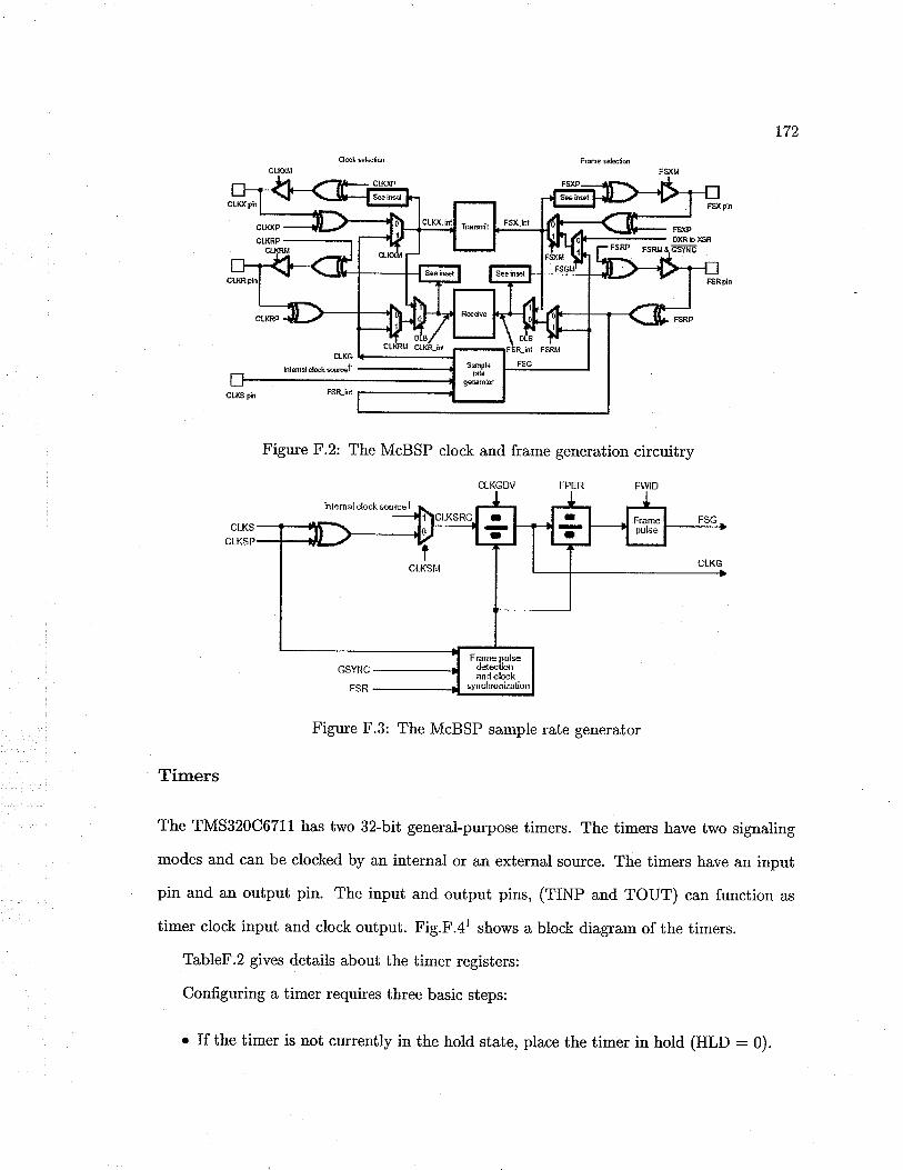
172
Cl@k ¡elælio FEme ¡elæliø
CtKG
inlmslctæk øut
Figure F.2: The McBSP clock and frame generation circuitry
C{-KGDV FPER FWID
Figure F.3: The McBSP sample rate generator
Timers
The TMS320C67LI has two 32-bit generai-purpose timers. The timers have two signaling
modes and can be clocked by an internal or an external source. The timers have an input
pin and an output pin. The input and output pins, (TINP and TOUT) can function as
timer clock input and clock output. Fig.F.4l shows a block diagram of the timers.
TableF.2 gives details about the timer registers:
Configuring a timer requires three basic steps:
o If the timer is not cu¡rently in the hold state, place the timer in hold (HLD : 0).
Fmme Dulsedettrtiqrand clock
synclrroniation

173
not change the GO
Figure F.4: The C67lI time¡s
Write the desired value to the timer period register (PRD).
o Write the desired value to the timer control register (CTL). Do
and HLD bits of ihe CTL in this step.
o Start the timer by setting the GO and HLD bits of the CTL to
In pulse mode operation, the output clock frequency is given by;
Frequency of clock source
1.
Perþheml Bus to CPU and D[.-tA
ïSTÂT. timeroulput Tlf'll limsiñltrrupl lo CPU and DlrlÄINVOUT
Frequency:Tí,mer peri.od reg'í,ster ualue
(F.1)

Table F.2: Ti
In clock mode operation, the output clock frequency is given by;
174
(F.2)D r Frequency of cloclc sourceÍ TeccJencu
2 * T,imer peri,od reg'ister aalue
IInEI rs
Timer0 Timerl Register Description
01940000
01940004
01940008
01980000
01980004
01980008
Timer Control
(crl,)
Timer Period
(PRD)
Timer Counter
(cNr)
Determines the operating mode of the timer,
monitors the timer status, and controls the
function of the TOUT pin.
Contains the number of timer input clock
cycles to count. This number controls the
TSTAT signal frequency.
Current value of the incrementing counter.

Acronyms
ADC Analog to Digital Converter
AI Artificial Intelligence
ALU Arithmetic Logic Unit
ANN Artificial Neural Network
API Application Programming Interface
ASIC Application Specific Integrated Circuit
CCVT Capacitor Coupled Voliage Tbansformer
CFR Con-figuration Register
CLKR Receive Clock
CLKX Tlansmit Clock
COFF Common Object File Format
CT Current tansformer
CWT Continuous Wavelet tansformDAC Digital to Analog Converter
DFT Discrete Fourier Tbansform
DLL Dynamic Link Library
DMA Direct Memory Access
DRR Data Receive Register
DSK Digitat Signal Processor Starter KitDSP Digital Signal Processor
DWT Discrete Wavelet Tlansform
DXR Data Tbansmit Register
EDMA Extended Direct Memory Access
EHV Extra High Voltage
EMIF External Memory Interface
L75
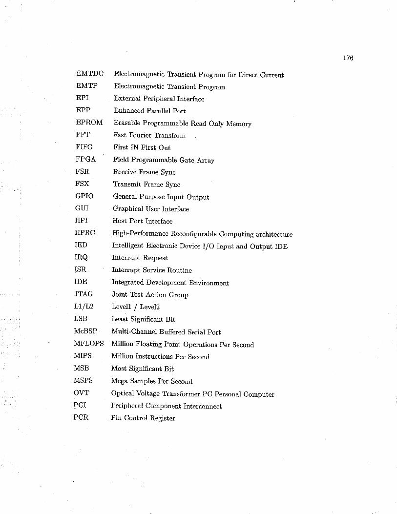
176
EMTDC Electromagnetic Tbansient Program for Direct currentEMTP Electromagnetic Tbansient Program
EPI External Peripheral Interface
EPP Enhanced Parallel Port
EPROM Erasable Programmable Read Only Memory
FFT Fast Fourier Tlansform
FIFO First IN First Out
FPGA Field Programmable Gate Array
FSR Receive Fbame Sync
FSX Tbansmit Flame Sync
GPIO General Purpose Input Output
GUI Graphical User Interface
HPI Host Port Interface
HPRC High-PerformanceReconfigurablecomputingarchitecture
IED Intelligent Electronic Device I/O Input and Output IDEIRQ Interrupt Request
ISR Interrupt Service Routine
IDE Integrated Development Environment
JTAG Joint Test Action Group
LIILL Levell f Level2
LSB Least Significant BitMcBSP Multi-Channel Buffered Serial port
MFLOPS Million Floating Point Operations per Second
MIPS Million Instructions Per Second
MSB Most Significant Bit
MSPS Mega Samples Per Second
OVT Optical Voltage Tbansformer pC personal Computer
PCI Peripheral Component Interconnect
PCR Pin Control Register
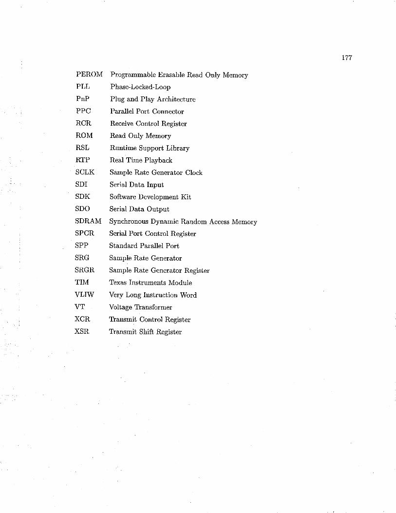
177
PEROM Programmable Erasable Read Only Memory
PLL Phase-Locked-Loop
PnP Plug and Play Architecture
PPC Parallel Port Connector
RCR Receive Control Register
ROM Read Only Memory
RSL Runtime Support Library
RTP Real Time Playback
SCLK Sample Rate Generator Clock
SDI Serial Data Input
SDK Software Development KitSDO Serial Data Output
SDRAM Synchronous Dynamic R¿ndom Access Memory
SPCR Serial Port Control Register
SPP Standard Parallel Port
SRG Sample R¿te Generator
SRGR Sample Rate Generator Register
TIM Texas Instruments Module
VLIW Very Long Instruction Word
VT Voltage Tbansformer
XCR Tbansmit Control Register
XSR Thansmit Shift Register
FÙeference
[1] D. Novosel, M.M. Begovic, and v. Madani, "shedding light on blackouts,,, IEEE power
and Energy Magazine,Yol.2, No.1, Jan/Feb 2004, pp.33-48
[2] J.s. Thorp, A.G. Phadke, s.H. Horowitz, and J.E. Beehler, ,,Limits to impedance
relaying", IEEE Tbansact'ions Pouer Apparatus and Systems, Vol.gg, No.l, Jan/Feb
t979, pp.246-256
[3] S.H. Horowitz, A.G. Phadke, and J.S. Thorp. "Adaptive transmission system relaying",
IEEE Transact'i'ons on Power Deliuery, vol.3, No.4, pp.1436-L445, oct lgg8
[4] L.V. Bewley, "Tïavelling waves on transmission systems", Dover Publications Inc., New
York, Second Edition, 1964
[5] P.A. Crossle¡ and P.G. Mclaren, '(Distance protection based on travelling waves,,,
IEEE Tlansactions Power Apparatus and System.s, vo1.102, No.9, Sep 1gg3, pp.2gz1-
2983
[6] P.A. Crossle¡ "Distance protection based on travelling waves", Ph.D. Thesis, Univer-
sity of Cambridge, Jan 1983
[7] E.H. Shehab-Eldin, "TYavelling wave distance measurement in E.H.V. power systems,,,
Ph.D. Thesis, University of Cambridge, Jan Lg88
[8] D.A. Douglass, "Current transformer accuracy with asymmetric and high frequency
fault currents", IEEE Tlansact'ions on Power Apparatus and, Systerns, Vo1.100, No.B,
Mar 1981, pp.1006-1012
[9] D.A. Douglass, "Potential transformer accuracy at 60Hz voltage above and below rating
and frequencies above 60H2", IEEE TYansact,í,ons on Power Apparatus and, Systerns,
VoI.100, No.3, Mar 1981, pp.13T}-1.gTs
L78

179
[10] Working Group 05 of Study Committee 36, "Tïansformers and instruments for mea-
suring harmonics", Electra, No.124, May 1g8g, pp.g2-g7
[11] N. Kehtarnavaz, and M. Keramat, "DSP system design using the TMSA20C6000",
Prentice Hall, 2001
[12] PSCAD/EMTDC Version 3.0 User Manual, Manitoba HVDC Resea¡ch Centre, lggg
[13] A.R. van c. warrington, "Protective relays", vol.l, chapman & Hall, 1g6g
[14] A.G. Phadke, and J.S. Thorpe, "Computer relaying for power systems,', John Wiley
& Sons Inc., 1988
[15] G.D. Rockefeller, "Fault protection with a digital computer", IEEE Ttransact¿ons on
Power Apparatus and Systems, Vol.88, No.4, Apr 1g6g, pp. 4gg-464
[16] B.J. Mann, and I.F. Morrison, "Digital calculation of impedance for transmission line
protection", IEEE Tlansact'i,ons on Power Apparatus and. Systerns, Vol.90, No.1, Jan
1971, pp. 270-279
[17] B.J. Mann, and I.F. Morrison, uRelaying a th¡ee phase transmission line with a digital
computer", IEEE Transacti,ons on power Apparatus and, Systems, vol.gg, No.2, Mar
I97L, pp.742-750
[18] G.B. Gilcrest, G.D. Rockefeller, and E.A. Udren, "High-speed distance relaying using a
digital computer" , IEEE Tlansact'i,ons on Power Apparatus and, Systems, Vol.gl, No.B,
May L972, pp. 1235-1243
[19] A.M. Ranjbar, and B.J. Cory, "An improved method for the digital protection of
high voltage transmission lines", IEEE Transactions on Power Apparatus and, Systems,,
VoI.94, No.2, Mar 7975, pp.544-550

180
[20] J.G. Gilbert, and R.J. Shovlin, "High speed transmission line fault impedance calcu-
lation using a dedicated mini computer", IEEE lhansactions on Power Apparatus and
Systems, Vol.94, No.3, Jun 1g25, pp.872-8g3
[21] Y. Miki, Y. Sano, and J. Makino, "Study of high-speed distance relay using microcom-
puter", IEEE Transacti,ons on Power Apparatus and, systems, vol.g6, No.2, Mar 1gzz,
pp. 602-613
[22] P'G. Mclaren, and M. Redfern, "Fou¡ier series techniques applied to distance protec-
tion", IEE Proceedings, Yo1.122, No.11, Nov 1g7b, pp.1801_1805
[23] M.S-sachdev and M.A.Baribeau, "A new aþrithm for digital impedance relays,,, IEEE
Tlransact'í,ons Power Apparatus and, sgstems, vol.gg, rg1g, pp.22}2-2240
[24] A.A. Girgis and R.G. Brown, "Application of Kalman filiering in computer relaying,,,
IEEE Transactions Power Apparatus and systems, vo1.100, 1gg1_, pp.BBgz-Jgg1
[25] M. Vitins, "A correlation method for transmission line protection" , IEEE Tlansacti,ons
Pouer Apparatus and systems, vol.gz, No.b, sep/oct 192g, pp.160z-1612
[26] M. Chamia, and S. Liberman, "Ultra high speed relay for EHV/UHV transmission
lines - development design and application", IEEE hansøctions Power Apparatus and,
Systems, Vol.96, No.6, Nov/Dec 1g7g, pp.2L04-21,I6
[2\ M. Vitins, "A fundamental concept for high speed relaying" , IEEE Tvansact¿ons on
Power Apparatus and Systems, Vo1.100, No.l, Jan 1gg1, pp.163_l6g
[28] D.W.P. Thomas, M.S. Jones, and C. Cristopoulos, "Phase selection based on superim-
posed component s", IEE Proceed,i,ngs on Generatí,on, hansmission and, Distri,bution,
VoI.143, No.3, May 1996, pp.2g5-2gg
[29] H.W. Dommel, and J.M. Michels, "High speed relaying using travelling wave transient
analysis", IEEE PES wi,nter Meeti,ng: N.y., ATg, Jan/Feb rg1g, pp.2!4-2Lg

181
[30] A.T. Johns, "New ultra high speed directional comparison technique for the protection
of EHV transmission lines", IEE Proceedings, yol.r27 pt.c, No.4, Jul 1gg0, pp.22g-2zg
[31] S. Rajendra, and P.G. Mclaren, "T]avelling-wave techniques applied to the protection
of teed circuits: Principle of travelling-wave techniques" , IEEE Tlansactions on power
Apparatus and Systems, Vo1.104, No.12, Dec 1g85, pp.85443550
[32] S. Rajendra, and P.G. Mclaren, "Tbavelling-wave techniques applied to the protec-
tion of teed circuits: Multi-phase/multi-circuit system", IEEE Transactions on power
Apparatus and Systems, Vo1.104, No.12, Dec 1g85, pp.Jbbl-8557
[33] M.M. Mansour, and G.W. Swift, "A multi-microprocessor based travelling wave relay
- theory and realization", IEEE Tlansact'ions on Power Del,iaery, Vol.l, No.l, Jan
L986, pp.272-279
[34] E.H. Shehab-Eldin, and P.G. Mclaren, "Tlavelling wave distance protection - problem
areas and solutions", IEEE T\ansactions on Pouer Deliuery, Vol.3, No.3, Jul 1g88,
pp.894902
[35] C. Christopoulos, D.W.P. Thomas, and A. V/right, "Scheme, based on travelling-waves,
for the protection of major transmission lines", IEE Proceed,,ings, Part C: Generation,
Tbansmissi,on and Distri,butiou Vol.L85, No.1, Jan 1ggg, pp.6J_ZB
[36] C' Christopoulos, D.W.P. Thomas, and A. Wright, "signal processing and discrim!
nating techniques incorporated in a protective scheme based on travelling waves,,, .IEE
Proceedi'ngs, Part C: Generation, Ihansmi,ss'i,on and Distribution, Vol.1B6, No.5, Sep
1989, pp.279-288
[37] G.B. Ancell, and N.C. Pahalawaththa, "Maximum likelihood estimation of fault lo-
cation on transmission lines using travelling waves", IEEE Tbansactions on power
Deliaery, Vol.9, No.2, Apr 1gg4, pp.680-68g

182
[38] Z.Q. Bo, M.A. Redfern, and G.C. Weller, "Positional protection of transmission line
using fault generated high frequency transient signals", IEEE Transactions on Power
Deliuery, Vol.15, No.3, Jul 2000, pp. 888-894
[39] J. Liang, S. Elangovan, and J.B.X. Devotta, "Pattern recognition technique for trav-
ellingwave protection", Electric Machi,nes and Power Systems, Taylor ü Franci,s Ltd,
London, Englnd, Vol.26, No.10, Dec 1998, pp.1007-1018
[40] J. Liang, S. Elangovan, and J.B.X. Devotta, "Adaptive travelling wave protection
algorithm using two correlation functions", IEEE Transactions on Power Deli,uery,
Vol.14, No.l, Jan 1999, pp.126-131
[41] A.G. Phadke, and S.H. Horowitz, "Adaptive relaying", IEEE Computer Applicati,ons
'ùn Power Magazine, Vol.3, No.3, JuI 1990, pp.47-51
[42] G.D. Rockefeller, C.L. Wagner, J.R. Linders, K.L. Hicks, and D.T. RizS "Adap-
tive transmission relaying concepts for improved performance", IEEE thansactions
on Power Del'i,uery, Vol.3, No.4, Oct 1988, pp.1446 - 1458
[43] S.H. Horowitz, A.G. Phadke, and J.S. Thorpe, "Adaptive transmission system relay-
ing", IEEE Transactions on Power Deli,uery, Vol.3, No.4, Oct 1988, pp.1436 - L445
[44] T.S. Sidhu, H. Singh, and M.S. Sachdev, "Design, implemetation and testing of an
artificial neural network based fault direction discriminator for protecting transmission
lines", IEEE Transactions on Power Deliuery, Vol.10, No.2, Apr 1995, pp.697-706
[45] D.V. Coury, and D.C. Jorge, "Artificial neural network approach to distance protection
of transmission lines", IEEE Tfansacti,ons on Power Deliuery, Vol.13, No.1, Jan 1gg8,
pp.102-108

183
[46] R. Venkatesan, and B. Balamurugan, "A real-time hardware fault detector using an ar-
tificial neural network for distance protection" , IEEE T\ansact'ions on Pouer Deliaery,
Vol.16, No.1, Jan 2001, pp.75-82
[471 O. Rioul, and M. Vetterli, "Wavelets and signal processing" , IEEE Sí,gnal Processing
Magazine, Vol.8, No.4, Oct 1991, pp.1438
[48] L.G. Weiss, "Wavelets and wideband correlation processing", IEEE Si,gnal Process'ing
Magazi,ne, VoLl1, No.1, Jan 1994, pp.13-32
[49] C.H. Lee, Y. Wang, and W.L. Huang, "A literature survey of wavelets in power engi-
neering applications", Proceed,i,ngs of the Nati,onal Sci,nce Counc,i,l, Republi,c of China,
Vol.14, No.4, 2000, pp.249-257
[50] D.C. Robertson, O.I. Camps, J.S. Mayer, and W.B. Gish, "Wavelets and electromag-
netic power system transients", IEEE Transact'ions on Power Del,í,uery, VoI.11, No.2,
Apr 1996, pp.1050-1058
[51] F.H. Magnago and A. Abur, "Fault location using wavelets", IEEE lTansactions on
Power Deliuery, VoI.1.3, No.4, Oct 1998, pp.1475-L480
[52] L. Shang, G. Herold, and J. Jaeger, "A new approach to high-speed protection for
transmission line based on transient signal analysis using wavelets", Deuelopments in
Power System Protection, 2001, pp.173-176
[53] X. Yibin, D.C. Wai, and W.W.L.A Keerthipala, "A new technique using wavelet anal-
ysis for fault location", S'i,rth International Conference on Deuelopments in Power
System Protection, Conf. Publ. No.434, Mar L997, pp.23l-234
[54] D.C. Wai, and X. Yibin, "A novel technique for high impedance fault identification",
IEEE Transactí,ons on Power Deliuery,Vol.13, No.3, Jul Lggl, pp.738-744

[55]
[56]
184
"The protective relay IED in the automation world", IEEE Power Engineering Society
Ttrtorial, 03TP162
Y. Serizawa, M. Myoujin, K. Kitamura, N. Sugaya, M. Hori, A. Takeuchi, I. Shuto,
and M. Inukai, "Wide-area current differential backup protection employing broadband
communications and time transfer systems", IEEE ITansactions on Power Deliuery,
Vol.13, No.4, Oct 1998, pp.1046-I052
J.C. Tan, P.A. Crossley, P.G.Mclaren, P.F. Gale, I. Hall, and J. Fa.rrell, "Application
of a wide area backup protection expert system to prevent cascading outages" , IEEE
Tbansactions on Power Deliuery, Vol.17, No.2, Apr 2002, pp.375-380
G.W. Swift, "The spectra of fault-induced transients", IEEE Transact'ions on Power
Apparatus and System.s, Vol.98, No.3, May/Jun, 1979, pp.940-947
[59] G.B. Ancell, and N.C. Pahalawaththa, "Effects of frequency dependence and line
parameters on single ended travelling wave based fault location schemes", IEE
Proceed'ings-Q Vo1.139, No.4, Jul 1992, pp.332-342
L.M. Wedepohl, "Application of matrix methods to the solution of travelling-wave phe-
nomena in polyphase systems", Proceedings of IEE, Vol.1-10, No.12, Dec 1963, pp.2200-
22L2
P.C. Magnusson, "Tlavelling waves on multi-conductor open-wire line - A numerical
survey of tbe effects of frequency dependence of modal composition", IEEE Transac-
tions Power Apparatus and Systems, Vol.92, No.3, May/Jun L973, pp.999-1005
K.G. Beauchamp, and C.K. Yuen, "Digital methods for signal analysis", George Allen
and Unwin Ltd, L979
[57]
[58]
[60]
[61]
[62]
[63] G.L. Richard, "Understanding Digital Signal Processing", Addisson \Mesley 1997
185
[64] W.H. Press, S.A. Teukolsky, W.T. Vetterling, B.P. Flannery, "Numerical Recipes in
Fortran 90", Cambridge University Press, Second Edition, 1996
[65] L.H. Christensen, "Design, construction, and test of a passive optical prototype high
voltage instrument transformer", IEEE Transactions on Power Delivery, Vol.L0, No.3,
Jul 1995, pp.1332-1337
[66] Real Time Playback User's Guide, Revision 1.1, Manitoba HVDC Research Center,
June 200L
[67] Dakar F5 Carrier Board Technical Reference, Spectrum Signal Processing Inc., Docu-
ment Number 500-00353, Revision 1.10, May 1998
[68] TMS320C4x User's Guide, SPRU063, Texas Instruments Incorporated, May 1998
[69] Dakar F5 Carrier Boa¡d (fser's Guide, Spectrum Signal Processing Inc., Document
Number 500-00354, Revision 2.11, October 1998
[70] Toolbox Configuration Utilities User Guide, Spectrum Signal Processing Inc., Docu-
ment Number 500-00409, Revision 1.00, June 1998
[71] Code Composer Studio v3.0 User's Guide, GO DSP Corporation, 1-gg8
[72] TMS320C4x C Sou¡ce Debugger User's Guide, SPRU054, Texas Instruments Incorpo-
rated, May 1992
[73] DL3-A1 DL3ADA100 Analog Module User Guide, Spectrum Signal Processing Inc.,
Document Number 500-00352, Revision 1.03, December 1gg8
[74] DSP-LINK3 Memory Mapped Expansion Bus Interface Specifications, Spectrnm giga¿t
Processing Inc., Revision 1.02, Nov 1998
[75] C6211 lC67Il DSK Hardware Installation Quick Start, SPRU436A, Texas Instuments
Incorporated, 2001
186
[76] C6211 lC67It DSP Starier Kit (DSK) Quick Start, SPRU437A, Texas Instuments In-
corporated, 2001
[77] TMS320C6000 Technical Brief, SPRU197D, Texas Instuments fncorporated, Feb 1999
[78] TMS320C6000 Peripherals Reference Guide, SPRU190D, Texas Instruments Incorpo-
rated, 2001
[79] Code Composer Studio Getting Started Guide, SPRU509, Texas Instruments Incorpo-
rated, 2001-
[80] Code Composer Studio Users Guide, SPRU328B, Texas Instruments Incorporated,
2000
[81] TMS320C6000 Code Composer Studio T\rtorial, SPRU301C, Texas fnstruments Incor-
porated, 2000
[82] TMS320C6000 Optimizing C Compiler flser's Guide, SPRU187I, Texas Instruments
fncorporated, 2001
[83] TMS320C6000 Assembly Language Tools User's Guide, SPRU186I, Texas Instruments
Incorporated, 2001
[84] TMS320C6000 Chip Support Library API Reference Guide, SPRU401B, Texas Instru-
ments Incorporated, 2001
[85] TMSS 20C62x DSP Library Programmer's Reference, SPRU402, Texas Instuments In-
corporated, 2000
[86] The C++ Programming Language, Third Edition, Bjarne Stroustrup, Addison-Wesley,
1999
[87] RIDE User's Manual, v4.2, Hyperception Inc., Jan 2001
[88] zuDE F\rnction Reference, v4.L,Hyperception Inc., Feb lgg8

187
[89] Visual C++ User's Guide, Version 6.0, Microsoft Corporation, 1999
[90] Data Converter Selection Guide, Texas Instruments Incorporated, 2001
[91] 12-bit, 4 Analog Input, 6 MSPS, Simultaneous Sampling Analog- to-Digital Converters,
SLAS217H, Texas Instruments Incorporated, May 1999
[92] THS1206EVM User's Guide, SLAU042B, Texas Instruments Incorporated, January
2001
[93] Designing with the THS1206 High-Speed Data Converter, SLAA094, Texas Instru-
ments Incorporated, April 2000
[94j TLV2548EVM 12-bit ADC EVM User's Guide, SLAU029A, Texas Instruments Incor-
porated, May 1999
[95] TLV2548, L2-bit,200KSPS, 8-channel, Low Power Serial Analog-io-Digital Converters
with Auto Power Down, SLAS198E, Texas Instruments Incorporated, February 1999
[96] Interfacing the TLV2544|TLV2548 ADC to ihe TMS320C5402 DSP, SLAA093A, Texas
Instruments Incorporated, October 2000
[97] TMS320C6000 EVM Daughterboard Interface, SPRA478, Texas Instruments fncorpo-
rated, December 1998
[98] TMS320 Cross-Platform Daughtercard Specification Revision 1.0, SPRA7L1, Texas
Instruments Incorporated, 2000
[99] TMS320 Cross-Platform Daughtercard Adapter, SLAU074, Texas Instruments Incor-
porated., May 2001
[100] TMS320C6000 Programmer's Guide, SPRU198F, Texas Instruments Incorporated,
2001
188
[101] TMS320C6000 McBSP Initialization, SPRA488, Texas Instruments Incorporated,
1998
[102] TMS320C6000 CPU and Instruction Set Reference Guide, SPRU189F, Texas Instru-
ments Incorporated, 2000
[103] Using the TMS320C5402 DMA Channels to Read F]om the TLV2548, SLAA095,
Texas Instruments Incorporated, 2000
[104] Interfacing the TLV2544|TLV2548 ADC to the TMS320C31 DSP, SLAA101, Texas
Instruments Incorporated, 2000
[105] ADS8364EVM User's Guide, SLAU084, Texas Instruments Incorporated, April 2002
[106] 4DS8364, 250kHz, 16-Bit, 6-Channel Simultaneous Sampling Analog-to-digital Con-
verters, SBAS219A, Texas Instruments Incorporated, June 2002
[107] Software Control of the 4DS8364, SLAA155, Texas Instruments fncorporated, August
2002
[108] A.G. Phadke, M. Ibrahim, and T. Hlibka, "Fbndamental basis for distance relaying
with symmetrical components", IEEE T\ansact'ions on Power Apparatus and Systems,
VoI.96, No.2, Mar i977, pp.635-646
[109] C.L. Wadhwa, "Electrical power systems", New Age Publications, Second Edition,
September 1991