Transportation disadvantage impedance indexing - CORE

Journal of Transport Geography 48 (2015) 61–75

Contents lists available at ScienceDirect

Journal of Transport Geography

j ourna l homepage: www.e lsev ie r .com/ locate / j t rg

brought to you by COREView metadata, citation and similar papers at core.ac.uk

provided by DSpace@IZTECH Institutional Repository

Transportation disadvantage impedance indexing: A methodologicalapproach to reduce policy shortcomings

Yavuz Duvarci a, Tan Yigitcanlar b,⁎, Shoshi Mizokami c

a Department of City and Regional Planning, Izmir Institute of Technology, Gülbahce, Urla, Izmir, Turkeyb School of Civil Engineering and Built Environment, Queensland University of Technology, 2 George Street, Brisbane, QLD 4001, Australiac Civil and Environmental Engineering, Kumamoto University, 2-39-1 Kurokami, 860-8555 Kumamoto, Japan

⁎ Corresponding author.E-mail addresses: [email protected] (Y. Duvarc

(T. Yigitcanlar), [email protected] (S. Mizoka

http://dx.doi.org/10.1016/j.jtrangeo.2015.08.0140966-6923/© 2015 Elsevier Ltd. All rights reserved.

a b s t r a c t
a r t i c l e i n f o
Article history:Received 25 November 2014Received in revised form 3 June 2015Accepted 18 August 2015Available online 1 September 2015

Keywords:Transportation disadvantagedSocial exclusionTransportation disadvantage-impedance indexPolicymakingSimulation modellingArao, Japan

Access to transport systems and the connection to such systems provided to essential economic and socialactivities are critical to determine households' transportation disadvantage levels. In spite of the developmentsin better identifying transportation disadvantaged groups, the lack of effective policies resulted in the continuumof the issue as a significant problem. This paper undertakes a pilot case investigation as test bed for a newapproach developed to reduce transportation policy shortcomings. The approach, ‘disadvantage-impedanceindex’, aims to ease transportation disadvantages by employing representative parameters tomeasure the differ-ences between policy alternatives run in a simulation environment. Implemented in the Japanese town of Arao,the index uses trip-making behaviour and resident stated preference data. The results of the index reveal thateven a slight improvement in accessibility and travel quality indicators makes a significant difference in easingdisadvantages. The index, integrated into a four-step model, proves to be highly robust and useful in terms ofquick diagnosis in capturing effective actions, and developing potentially efficient policies.

© 2015 Elsevier Ltd. All rights reserved.

1. Introduction

The research conducted over the last decades resulted in identifyingthe major problems and locations of socially excluded (in broad terms,peoplewith the lack of participation in the economic, political and sociallife of the community) and transportation disadvantaged (TDA)(in broad terms, people that are prevented from participation inthe economic, political and social life of the community because of thereduced accessibility to opportunities, services and social networks)groups (Litman, 1997; Schlossberg, 2004; Duvarci and Yigitcanlar,2007; Delbosc and Currie, 2011a; Blair et al., 2013; Kamruzzamanet al., 2015; Rashid andYigitcanlar, 2015; Schwanen et al., 2015). As a re-sult, many cities around the globe develop policies in order to meet theneeds of these groups (Battellino, 2009). Utility of new technologies andhigh capacity computers are seen as support tools in these policymakingefforts (Yigitcanlar et al., 2010). However, estimating the effectivenessof policies beforehand is immensely critical, where this can be achievedby implementing cost-effective simulationsusing transportationmodels(Kamruzzaman and Hine, 2011; Kamruzzaman et al., 2014). Yet, up-to-date travel demand model software packages have neglected to incor-porate social considerations and the required equity parameters, even

i), [email protected]).

for the neediest—i.e., disabled and elderly (Banister, 2002; Delbosc andCurrie, 2011b; Lucas, 2012; Wasfi et al., 2012).

Furthermore, as emphasised by Lucas (2012, 112), “if properlydesigned and delivered, public transport can provide a part of [theTDA] solution, but it is most likely that other forms of more flexible(and often informal) transport services will be needed to complementthese mainstream services. [Nonetheless,] this does not come cheap.”Consequently, insufficient funds, high costs of special treatment ofTDA, and costly provision of the special services enforce policymakersto look for cost-effective, timesaving, appropriate, and applicable solu-tions (Metz, 2003). Simulation models provide opportunity to testpolicy effectiveness before their implementation (Barceló, 2010); how-ever, at present there are no straightforward policy simulation applica-tions in the TDA domain.

The primary aim of this research is to develop an indexing approach,‘disadvantage-impedance index (DIX)’, to fill this gap. Travel ‘imped-ance’ to the nearest service, in distance or time, is a commonly usedmeasure of spatial accessibility (see McGrail and Humphreys, 2009).The term is also used to refer to transport related disadvantageoussituations travellers experience such as very long walking distancesto/frompublic transport stops or poor quality of public transport system(see Bunker et al., 2015). DIX is developed through the adjustmentof modelling routine, as existing software are restricted in effectivepolicymaking due to neglected social considerations. This indexingapproach enables obtaining the best policy measures requiring onlysingle-shot collected data in utilised cyclic run iterations. In DIX, stated

https://core.ac.uk/display/324142523?utm_source=pdf&utm_medium=banner&utm_campaign=pdf-decoration-v1

http://crossmark.crossref.org/dialog/?doi=10.1016/j.jtrangeo.2015.08.014&domain=pdf

http://dx.doi.org/10.1016/j.jtrangeo.2015.08.014

mailto:[email protected]



http://dx.doi.org/10.1016/j.jtrangeo.2015.08.014

http://www.sciencedirect.com/science/journal/

www.elsevier.com/locate/jtrg

62 Y. Duvarci et al. / Journal of Transport Geography 48 (2015) 61–75

preference data technique (P.data) is used to obtain detailed informa-tion from the population, for better and quicker policy capturing,instead of blind trials for finding best policies. This approach aims toprovide a solution to represent TDA views in policy determination.Therefore, it utilises mixed stated preference and revealed preferencesurvey techniques, to understand traveller reactions against variouspolicy scenarios, and helps inclusion of the user preferences, and thusenables participation of TDA in the policymaking process containingdifferent scenarios and solution options (Lam and Xie, 2002; Alver andMizokami, 2006; Duvarci and Mizokami, 2009). Investigating the com-patibility of the approach to commercially available mainstreamsoftware—i.e., JICA-STRADA—is the secondary aim of this research.

2. Literature review

The common characteristics of disadvantaged populations areextensively discussed in the literature—see Church et al. (2000), Hineand Grieco (2003), Hine and Mitchell (2003), Duvarci and Yigitcanlar(2007), and Duvarci et al. (2011). While mostly used interchangeably,TDA and transport-related social exclusion are not necessarily synony-mous with each other. For instance, a socially excluded can have goodaccess to public transport options or a transport disadvantaged can besocially included (see Stanley and Vella-Brodrick, 2009; Delbosc andCurrie, 2010). According to Lucas (2012, 106) “rather [TDA] and socialdisadvantage interact directly and indirectly to cause transport poverty.This in turn leads to inaccessibility to essential goods and services, aswell as ‘lock-out’ from planning and decision-making processes, whichcan result in social exclusion outcomes and further social and transportinequalities will then ensue”. Not only personal and socioeconomicreasons (Licaj et al., 2012), but also the transport system itself canhave a crucial role in creating barriers (Church et al., 2000). Hine andGrieco (2003) argue that combination of poor accessibility with lowlevels of mobility, and low levels of sociability intensifies the socialexclusion. According to Lucas (2006) among the TDA categories, theelderly and disabled deserve more attention.

Many countries—i.e., Sweden, Canada, and Australia—have alreadylaunched legislations requiring improvements in transportation ser-vices such that all members of the society have equity in accessibilityand mobility (Currie et al., 2009; Dodson et al., 2010; Engels and Liu,2011; Jones, 2011). France, Spain, Canada, New Zealand, and SouthAfrica are responding to the TDA agenda, and without directly callingit TDA policy, the USA, Germany and the Netherlands offer policies toaddress the transport needs of disadvantaged groups (Lucas, 2012).The success factors are among the most popular issues for effectivepolicy solutions for TDA groups (Rau and Vega, 2012). Developing spe-cial infrastructure (e.g., technology equipped special services) for aidingTDA groups (especially disabled and elderly) is needed; however, itbrings additional cost to local authorities, which is a major obstacle inimplementation (Mokhtarian et al., 2006). Developing appropriatepolicieswith support of technology is amuchmore cost-effectivemethodin aiding those vulnerable groups (Nicolle and Peters, 1999; Duvarci andMizokami, 2007; Yigitcanlar and Kamruzzaman, 2014), which requiresdetailed information such as travel demands, preferences, modes andpaths of the population.

Gaining information about the TDA groups is necessary to identifyand document their accessibility and mobility needs (Lucas, 2011;Power, 2012), which can be suitably acquired through four-step traveldemand modelling. The importance of planning integrated to traveldemand models has been ignored in the contemporary efforts due tounawareness and lack of coordination between social institutions,including health and transportation service authorities. Nevertheless,the ability to configure proper policy measures to help improve theTDA is of prime importance for policymakers to lessen the avoidablecosts for both operators and users (Diana, 2004).

Measurement and level of analysis difficulties arise in TDA studiesdue to the multi-dimensionality of TDA. However, in some of the TDA

studies (Duvarci and Yigitcanlar, 2007; Duvarci et al., 2011), thesemethodological issues were addressed by using P.data. This helped indetermining the degree of disadvantages in social and geographicalterms. There is a need for developing a clear methodological approachto determine appropriate policies to decrease disadvantages—makingTDA people equal or close to non-TDA (NTDA) population in terms oftheir travel characteristics and opportunities. However, while providingsolution to TDA problem, it carries the risk of increased demand onthe road network causing congestion. Fortunately, a simulation study(Duvarci and Mizokami, 2007) reveals that even in the case of removalof all disadvantages, releasing suppressed trips of TDA would not causea burden on existing road infrastructures.

3. The disadvantage-impedance indexing approach

The disadvantage-impedance Index (DIX) is developed with an aimto compare available policies to improve TDA's travel conditions andtest effectiveness of these policies in a simulation environment. Thestructure and cycling process of the indexing approach are shown inFig. 1. The data used in the index is clustered as TDA andNTDA. Informa-tion from P.data, fed by the current (t time) clustering results of TDA,guides the choice of appropriate policy areas to focus on. Convincedthat improvements through simulations (both in terms of significantlyeasing the disadvantages and network congestion) are satisfactory toreduce the gap between TDA and NTDA, indicator index values areconverted to composite index values (DIX) and should be treatedfor observing new cluster analysis (t + 1 time) results. This is to testwhether the TDA population changed and the gap (cluster centreresults) is further reduced. The process stops, if the goal is achieved,and the best solution scenario is nominated. Only the changing P.datavalues—along with TDA profile improvements at each cycle—areapplied to the same modelling values.

The clustering process of the index is a dynamic one, and its resultsare expected to change (improvement for TDA) after each iterationcycle. Hence, the index always uses the same data in normalised indexvalues for convenience of input–output cycle operability, and for reduc-ing complexity. As stated by Parumog et al. (2008) using the improve-ment ratios as the common measurement between non-comparableindicators is a suitable technique for normalisation of values. In thelight of the new TDA evaluation routine—using cluster analysis, P.data,input of DIX indicators—improvements in the travel demandmodellingstructure of a commercial transport modelling software (i.e., JICA-STRADA) are elaborated as below.

Improvements made through simulations in the original zonal DIXare achieved by: (i) Obtaining the improvement rates by zones andindicators, and; (ii) converting the improvements into averaged ratevalues by zones to be added to the respected indicator index values.The ratio change of TDA out of total population, as a result of the nextclustering cycle, is a concern for evaluating performance of the system.This ratio change would not be a sole evaluator when the ratio of TDAcan get even larger than the previous case, if its conditions are improvedbecause of the increased numbers of TDA getting closer to NTDA. Thus,the metric gauge used for the improvement should be the reducedgap between overall cluster centre values of the two populations(increase in the TDA's cluster centre value) instead of the number ofTDA people. Cluster centre values of each indicator for each zonecan be used as a gauge to measure the improvement. If cluster centrevalues of TDA and NTDA converge to a negligible difference (5%), theprocess and the search for equalisation of TDA to NTDA should bestopped, and the finalised simulation results should be reviewed forpolicy analysis. The Pareto optimality condition is reserved such thatany increase in DIX can only rise up to that of NTDA; if exceeded, imbal-ance of disadvantage would be borne, avoiding equity. The way to sortout the best policies within this mechanism is beyond the scope ofthis paper.

Fig.1. Structure and cyclic process of the disadvantage-impedance indexing approach.

63Y. Duvarci et al. / Journal of Transport Geography 48 (2015) 61–75

4. Methodology of the approach

4.1. Indicator base

The approach has two types of indicators—composite and individualindicators. Indicators are selected as a result of the following consider-ations: (i) Lead of the literature; (ii) use of indicators practically asboth input and output—meaning that data is recycled and alteredfrom one iteration cycle to another to be used as an input for the nextsimulation round. This approach is followed mainly due to inconve-nience of frequent data collection from the field; (iii) indicator valuesto explain the reasons behind being of disadvantaged—for instance,disability should not be considered as a TDA factor, if the transportationsystem is adequate in accommodating them appropriately, and; (iv)compatibility with commercial travel demand software—i.e., JICA-STRADA.

The approach contains five composite indicators—i.e., accessibility(Access), land use and environmental conditions (LandEnv), physicalbarriers (PhysBarr), travel quality and comfort (TravQual), and trans-port system satisfaction and bus-stop conditions (TrSysQual). For eachcomposite indicator a number of individual indicators are assigned—atotal of 30 indicators (Table 1). These composite and individual indica-tors correspond to the most basic and essential elements of TDA and

are driven from the key literature (e.g., Ewing et al., 1996; Thompson,2001; Duvarci and Yigitcanlar, 2007; Yigitcanlar et al., 2007; Loaderand Stanley, 2009; Currie et al., 2010; Delbosc and Currie, 2011b,2011c; Kamruzzaman andHine, 2012; Schwanen et al., 2015). As acces-sibility plays a significant role in a person's TDA status, in this approach,accessibility to transport is, with some nuances, placed under the com-posite indicators of ‘TravQual’ (distance to the nearest public transportstop) and ‘TrSysQual’(distance to available public transport modes)rather than ‘Access’. The indicator structure of the DIX is presented inTable 3. Data required for these indicators are collected through ahousehold travel survey. Appendix 1 presents the survey questionnaire.

In obtaining recyclable data values across all indicators, normalisa-tion plays a central role that is conveniently realised by standardisationof all non-categorical data to adjust their values measured on differentscales to a notionally common scale. For the normalisation techniqueMin–Max-Scaling is used as a means that one linearly transforms realdata values such that the minimum and maximum of the transformeddata to take certain values between 0 and 100. The main reason ofchoosing this technique over others (e.g., z-score that normalisesbased on the mean; or decimal scaling that normalises by moving thedecimal point of values) is thatMin–Max-Scalingpreserves the relation-ships among the original data values. For categorical data, normalisationof all index indicator values to a five-scale system (i.e., lowest, low,

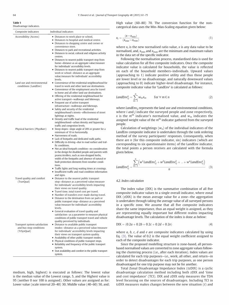
Table 1Disadvantage indicators.

Composite indicators Individual indicators

Accessibility (Access) ▪ Distances to work place or school,▪ Distances to hospital and medical centre.▪ Distances to shopping centre and corner or

convenience store.▪ Distances to park and recreational activities.▪ Distances to social, cultural and religious activity

centres.▪ Distances to nearest public transport stop from

home—distance as an aggregate value/measurefor individuals' accessibility levels.

▪ Distances to nearest public transport stop fromwork or school—distance as an aggregatevalue/measure for individuals' accessibilitylevels.

Land use and environmentalconditions (LandEnv)

▪ Convenience of the residential neighbourhood fortravel to work and other land use destinations.

▪ Convenience of the employment area for travelto home and all other land use destinations.

▪ Offering of the residential neighbourhood foractive transport—walkways and bikeways.

▪ Frequent use of active transportinfrastructure—walkways and bikeways.

▪ Safety and security of the residentialneighbourhood's streets—effectiveness of streetlightings at nights.

▪ Density and traffic load of the residentialneighbourhood—urban density and bypassingtraffic and congestion levels.

Physical barriers (PhysBarr) ▪ Steep slopes—slope angle of 20% or greater for aminimum of 10 m horizontally.

▪ Narrowness of roads.▪ Lack of footpaths and dedicated walk paths.▪ Difficulty in driving—due to road surface and traf-

fic conditions.▪ Not an ideal footpath condition—no consideration

in the design for disabled people and parentswithprams/strollers, such as non-dropped kerbs,width of the footpaths and absence of natural orbuilt protection elements from weather condi-tions.

▪ Traffic lights and long waiting times at crossings.▪ Insufficient traffic and road condition information

and signs.Travel quality and comfort(TravQual)

▪ Distance to the nearest public transportstop—distance as a perceived value/measurefor individuals' accessibility levels impactingtheir views on travel quality.

▪ Travel time, total travel cost per travel.▪ Number of transfers ever made during travel.▪ Distance to the destination from car park or

public transport stop—distance as a perceivedvalue/measure for individuals' accessibilitylevels.

▪ General evaluation of travel quality andsatisfaction—as a parameter to measure physicalconditions of public transport travel and vehiclequality perceived by individuals.

Transport system satisfactionand bus-stop conditions(TrSysQual)

▪ Distance to available public transportmodes—distance as a perceived value/measurefor individuals' accessibility levels impactingtheir views on transport system quality.

▪ Availability of other public transport modes.▪ Physical conditions of public transport stops.▪ Reliability and frequency of the public transport

system.▪ Seat availability and comfort in the public transport

system.


medium, high, highest) is executed as follows: The lowest valueis the median value of the Lowest range, 5, and the Highest value is95 (neither 0 nor 100 is assigned). Other values are assigned as for:Lower value (scale interval 20–40) 30; Middle value (40–60) 50, and;

High value (60–80) 70. The conversion function for the non-categorical data uses the Min–Max-Scaling equation given below:

xi ¼ x−xminð Þxmin−xmaxð Þ ð1Þ

where xi is the new normalised ratio value, x is any data value to benormalised, and, xmin and xmax are the minimum and maximum valuesin the data set of the specific indicator.

Following the normalisation process, standardised data is used forvalue calculation for all five composite indicators. Once the compositeindicator value is calculated for households, the value is reflectedon each of the household members–individuals. Upward values(approaching to 1) indicate positive utility and thus those peopleare lower level or no disadvantage, and naturally downward values(approaching to 0) indicate higher-level disadvantage. For instance,composite indicator value for ‘LandEnv’ is calculated as follows:

LandEnvni j ¼Xn

m¼1

wmxm for∀m ∈ n ð2Þ

where LandEnvij represents the land use and environmental conditions,where i and j indicate the surveyed people and zone respectively,x is the mth indicator's normalised value, and wm indicates theassigned weight value of the mth indicator gathered from the surveyedpeople.

Calculation of weightings (wn) of the individual indicators of theLandEnv composite indicator is undertaken through the rank orderingmethod of the survey participants' responses. Consequently, whenthere are n (for this composite indicator, six) indicators (which arecorresponding to six questionnaire items) of the LandEnv indicator,the total points a person receives are calculated with the formulagiven below.

LandEnvni j ¼

Xn

m¼1

w1LandEnv1i j þw2LandEnv2i j þ ::þwnLandEnvni j� �

nð3Þ

4.2. Index calculation

The index value (DIX) is the summative combination of all fivecomposite indicator values to a single overall indicator, where zonalDIX (zDIX) is the mean average value for a zone—the aggregationis undertaken through taking the average value of all surveyed personsin a specific zone. We assume that all five composite indicatorsshare the same importance, thus an equal weight is assigned, as theyare representing equally important but different realms impactingdisadvantage levels. The calculation of the index is done as below:

DIX ¼ 0:2aþ 0:2bþ 0:2cþ 0:2dþ 0:2eð Þ ð4Þ

where a, b, c, d and e are composite indicators calculated by usingEq. (3). The value of 0.2 is the equal weight coefficient assigned toeach of the composite indicator.

Since the proposed modelling structure is zone-based, all person-based normalised values are converted to zone aggregate values follow-ing the clustering process (i.e., after each iteration). Index values arecalculated for each trip purposes—i.e., work, all other, and return—inorder to detect disadvantages for each trip purposes, as one persondisadvantaged for one trip purpose may not be for another.

Total Zonal Disadvantage Impedance Index (tzDIX) is a cyclicdisadvantage calculation method including both zDIX and ‘timeand cost impedance’ (TCI). DIX and zDIX only measures the TDAlevel focussing on the sources of disadvantages. Including TCI intzDIX measures makes changes between the new situation (t) and


the previous case (t-1). The reason for insertion of all population'sTCI in the measurement system is that inclusion of all generalisedcosts is borne by the increase in TDA's travels. The travel demandsoftware utilising OD matrices calculates the TCI impedance easily.Nevertheless a separate calculation for TDA and NTDA is not possibleas both comprise non-separable traffic on a network. Disadvantageindicator impacts can be measured only after observing simulationapplications as model outputs. zDIX, however, is pre-determinedfrom P.data as a probability of conditions. In Eq. (5), zDIXs are placedat the left hand side and the trip impacts (usually cost as TCI) are atthe right hand side of the impact calculation. Since trip rate increaseand modal shift to public transport mode are perceived as positivecontributions, these impacts are not included in the disadvantageimpedance calculation. Evidently, most of the time TCI change hasa negative sign when improvements were made in the zDIX side, to-gether with supposedly increased trip rates, causing more conges-tion and delays in the system as a price of the improvement anddecreased ‘level of service’ (LOS). Thus, extra traffic load can have anegative impact (such as congestion) on the TDA's situation, andshould be subtracted from the improvement (positive side) of thezDIX, when trip rate or travel time increases.

tzDIXt ¼ zDIXt þ −ΔTCIð Þð Þ ¼ zDIXt−ΔTCIð Þ ð5Þ

where Δ represents the difference between the t and t-1 times in policyscenarios. Only the initial tzDIX does not contain TCI component as thereis no result of zDIX impact at this stage.

Since the tzDIX calculations are origin-based, all origins' impedancechanges (from t-1 to t time) to all destinations to be aggregated andaverage changes to be taken into account as shown in the followingequation:

TCIi ¼

Xj

Ii j� �

Z jð6Þ

where Zj is the total number of destination zones, j indicates all destina-tions and I is the classical TCI impedance difference.

4.3. Clustering process

In this study, simple K-means type clustering technique is used inthe cyclic modelling for improving the simulation results. K-means is atechnique that partitions observations into K clusters in which eachobservation belongs to the cluster with the nearest mean and thusserving as a prototype of the cluster. This clustering technique requiresdefinition of K numbers of clusters from the beginning, at which eachcluster to have intra-class similarity. The algorithms begin with a bestguess on the solution, and then refine the positions of cluster centres(i.e., TDA, NTDA) until reaching an optimum position. Clustering helpsas a control tool (monitoring improvements in TDA's position control-ling new condition-borne results) throughout the simulation cycles,and determines the new TDA groups (and its data) at each iterationcycle.With this process each of the succeeding iterations, that is a policyrecommendation, produces a reduced TDA group with an improvedoutcome. Clustering plays a critical role as an objective function of theDIXmethodology in finding the best solution through a systematic sim-ulation evaluation, and reducing undesired results, just on the basis ofmonitoring the differences between NTDA and TDA's cluster centrevalues. This process is shown below:

Min CtTDA– Ct

NTDA →stop process if CtTDA– Ct

NTDAb0:05→ iteration should continue if Ct

TDA– CtNTDAN 0:05

ð7Þ

where C is the overall cluster centre value (of all indicators, as in theoutput report of IBM-SPSS), with t representing the tth time iteration,and superscript TDA showing the result of TDA groups, and NTDA ofNTDA. Stability of the initial cluster centre results was not tested, tosee whether clustering results would be different if they were to bechanged, since the algorithm already seeks the best locations of thecentres through the applied process. Each time clustering is executedas a result of simulated policy intervention different populations ofTDA will form and impacted by the new situation's travel conditions.Consequently selecting new policies produces new P.data—to be usedin the next simulation cycle.

4.4. Policy simulation

Policy simulations serve two purposes in the context of thisstudy. The first purpose is to monitor the situation of the disad-vantaged by the aid of the P.data evaluation, supported by the re-clustering process that runs or stops the cycling process, and; seethe costs and impacts of assumptive policy applications in the im-provement of TDA's travels from the current situation. The secondone is to maintain Pareto optimality, and that the proposed situationshould not cause more congestion (considering only LOS) than thecurrent situation. The assignment results are required for controllingthe Pareto optimality condition on the network through the LOSindicator.

4.5. Data requirement

Anewmethod of simulation is devised for the study as a result of theincompatibility issue of the existing method in the travel demandsoftware—i.e., JICA-STRADA. In this newmethod the indicators (columns)and the trip impacts (rows) in the P.data matrix for each zone share thesame preference rates in measuring both total improvements in TDAand total trip impacts as rates. A similar approach is used, by Lam andXie (2002), in preference modelling of path choices of transit users forSingapore to determine transit paths if the conditions of transportationare to be improved using mixed stated and revealed P.data techniques.This exercise revealed that the single criterion of impedance is sufficientin choosing path or mode.

Impedance is not solely made up of time and cost. The novel idea ofthe study is based on the assumption that change in the travel situationof those TDA by each improvement caused by new policy scenariosdependently changes the satisfaction levels and preferences of thisgroup. P.data provides the information, for some determined set ofhypothetical conditions (which are identical with TDA indicators), onwhat the probability of changewould be (trip rate doubles, costs reduceby half, or increase public modes or cycling). These probabilities areused later as the measure of impact for such policies. Disadvantagelevels and probability shares, and thus their P.data, are expected tochange each cycle, as depicted in Fig 2. The preference probabilitiesare zone-aggregated for convenience. Once collected precisely, P.dataguides simulations assuming that respondent preferences and reactionswill remain constant over time.

It is essential that the stated preferences show the degree of proba-bility that the chosen policy is most likely to be successful as far asthe surveyed people's responses are reliable. By answering ‘yes’ as oneoption among the others (see Appendix 1 Part F), respondent readily as-sumes their disadvantage related to the condition that will besignificantly reduced or removed once a solution is provided. At thesame time, the improvements are most likely to cause impacts on thesystem such as increased trip rate, which will affect the next iteration.Not all people in the zone select to that particular option, somewill pre-fer other impact options, and thus, accepting the option will be a gaugefor TDA improvement. The degree of reducing disadvantages will varyacross the indicators. Finally, for the combined index value, all obtainedvalues from each indicator are summed up.

Fig. 2. Calculation procedure of disadvantage improvement rates.


All participant responses are aggregated in the form of P.datamatrices for each zone, columns showing index items (if-condition) ofdisadvantages and rows showing the possible trip impacts against the‘if’ conditions. ‘Yes’ responses of those who already satisfy the conditionare eliminated—e.g., a person who already travels by bike answering‘yes’ for the question of ‘Do you prefer your travel mode to be walk-ing or cycling?’ is conflicting, thus their evaluation is removed. Thezone-aggregated values from respondents in a zone are referred as‘zonal preference’ or ‘impact’, and calculated as follows:

Idi ¼X

pyp for∀ i ∈ Z ð8Þ

Fig. 3. Location

for y = 1, if y = ‘yes’ selection exists for TDA, where I representszonal impact value, i the counter of zone (Z), d the counter of TDAperson in zone, and p the number of persons surveyed.

P.data matrix evaluation requires a set of rules for efficient goal-oriented impact evaluation. One such adopted rule is satisfying optimumimpact between indicators and trip impacts regarding to higher total im-pacts (above a defined value, or based on defined number of highest col-umn and row sums) ever observed. Accordingly, the impact evaluation isbased on two constraints: Indicators, and trip impacts. The total sum(i.e., improvement) should not exceed 100% impact in a run, as for Paretooptimality is concerned—or improvement rates should be introduced in-crementally. For realistic probabilities, the final improvement rate

of Arao.

Fig. 4. Road network and public transport routes in Arao.

Table 2Household survey summary.

Zonenumber

Zone name Population Responserate

Sampleratio

Disable population& rate

1 Yotsuyama 5577 98 0.018 18 (%18)2 Manda 4948 86 0.017 12 (%14)3 Ide 5184 172 0.033 31 (%18)4 Hirayama 2357 60 0.025 6 (%10)5 Kunai 2,930 123 0.042 21 (%17)6 Arao Centre 7217 101 0.014 9 (%9)7 Midorigaoka 896 65 0.072 6 (%9)8 Masunaga 5407 103 0.019 17 (%16)9 Kawanobori 4846 69 0.014 16 (%23)10 Sakurayama 3032 46 0.015 8 (%17)11 Hatimandai 3084 45 0.015 10 (%22)12 Ariake 3399 116 0.034 22 (%19)13 Kiyosato 2965 82 0.028 4 (%5)14 Hatiman–Yahata 3538 142 0.040 15 (%11)15 Fumoto 1525 33 0.022 5 (%15)Total 56,905 89.4 0.024 200 (%15)


determined is multiplied by the cell's base occurrence probability—sincethere are five if-condition (composite) indicators and five impact reac-tions,whichmakes 25 possibilities of different impacts (i.e., 1/25 numberof cells in the matrix: 0.04).

5. Pilot application of the approach

5.1. Study area

The test bed town—Arao, a former mining town highly regarded asan important contributor to Japan's modernisation, and in declinesince the closure of the coal mines in the late 90s—is chosen for itshigher rate of elderly, disabled, and potentially TDA population,dispersed settlement structure, and heavily car-based transportationsystem that may cause barrier effect to TDA. The town is establishedon a land of about 5700 ha and has a population of 56,822 (in 2012)with 24,255 households and the density of about 9.97 persons/ha. TheIshaya Bay houses Arao in the northwest part of the Kumamoto Prefec-ture about 35 km from the city of Kumamoto (Fig. 3). Arao has ascattered settlement character, denser in two central areas, namelyMidorigaoka and Yotsuyama. Average household size is 2.34. The elder-ly population ratio (above 65 years old) is 36.4%—well above the nation-al average of 31.3%. Unemployment rate (9.1% of the working agepopulation) is quite high compared to other parts of Japan. Arao is cur-rently served with 29 public transport routes one being intercity trainline and the rest bus network, where five of them are intercity routes(Fig. 4).

5.2. Data collection and analysis

A household travel survey is conducted to obtain necessary data totest run the indexing approach in Arao between April and May 2012.In total 1069 households are invited to take part in the household travelsurvey that contains 56 questions (see Appendix 1). The selection of

the households is done based on the stratified random samplingmethod—considering the age, gender and income levels of the districtsof Arao. The self-administered surveys are conducted through postalmail, and executed for each member of the household. The surveydata are parted into two groups as general household-level data forhousehold specific information and personal data for individual specificinformation. Among those invited 663 responded to the survey (62%response rate), where 627 of valid responses are processed, whichequates to 1342 individuals with 2.4% sampling rate,making an averageof 89.5 observations per zone—total of 15 zones (Table 2). Through thisexercise, travel characteristics of participants—trip details for the weekprior to the survey—are captured along with their preferences for TDA

Table 3Travel characteristics of Arao.

Trip rate by purpose Trip rate by mode Modal share Average trip length and cost Number of transit lines Traffic problems

Work: 0.67All other: 0.73Return: 0.69Total: 2.13

Walk & cycle: 0.25Private: 1.61Public: 0.13

Walk & cycle: 13%Private: 81%Public: 7%

Work: 12.1 km/282¥All other: 10.5 km/217¥Return: 11 km/276¥

23 inner and6 external

Peak hour congestion incentral locations


indexing. Of the sampled population, overall household size is 2.7,average age is 50.5, gender distribution is 51% female and 49% male,car ownership per household is 1.85 (self-owned automobile and/orcompany car), bicycle and/or motorcycle ownership is 1.51, and annualaverage household income per capita is JPY 3,215,236 (about USD27,000). Major trip purposes used in this study are ‘work’ (composedof commuting and business trips), ‘all other’ (all social, recreational,and health related trips), and ‘return’ trips (all home returning trips).The OD data of all trips and mode combinations are formed. Majormodes used are ‘private’ (private car, ride given,motorbike trips), ‘public’(bus, train), and ‘walk & cycle’ trips (Table 3).

DIX values are obtained to measure disadvantage levels in terms offive pre-defined composite indicators, and are used as zone aggrega-tions (mean averages). After calculating DIX values for each compositeindicator, they are ready for the cluster analysis for determining TDA.The initial cluster centre results, based on five composite indicatorsand different trip purposes are presented in Table 4. For work trips,there are 699 persons assigned to the TDA category out of 1341 (52%of all population), while the figure for all other trips is 633 persons(47%). Return trips are omitted from analysis due to inconsistency inthe results—i.e., ‘TravQual’ indicator not providing reliable findings forTDA in return trips. According to the cluster centre results TDA is notdisadvantaged in terms of ‘TrSysQual’ indicator for all trip purposes.Thus, in the P.data evaluation and related simulation stage, this indicatoris discarded. Based on these findings it is possible to say about half of theArao people are TDA (see Fig. 5).

Table 4Cluster centre results.

Cluster centrevalue for ‘work’

Cluster centrevalue for ‘all other’

Cluster centrevalue for ‘return’

TDA NTDA TDA NTDA 1⁎ 2⁎

Access .47 .86 .48 .70 .61 .87LandEnv .43 .74 .44 .60 .55 .76PhysBarr .57 .85 .60 .95 .34 .80TravQual .84 .90 .86 .91 .85 .82TrSysQual .83 .62 .88 .66 .86 .59Overall .60 .81 .62 .84 .64 .77

⁎ The cluster could not be classified as TDA or NTDA.

5.3. Traffic assignment

This study only concerns of the traffic assignment stage of the classi-cal four-step modelling since the impacts of current traffic are investi-gated. Taking only the last stage of modelling is meaningful because ofthe sufficiency of this stage in terms of operable parameters is used insimulations free from the other modelling stages. The transit assign-ment is also required for interaction between model's inputs and out-puts. The necessary data for the current traffic assignments includesmode and purpose matrices of both TDA and NTDA populations,and their impedance matrices (min. route distance impedance), whichadds up to 15 OD matrices in total, each calculated in JICA-STRADA.Separate cost data are used for private and public mode choice models.The focus trip purposes are ‘work’ (commuting and business) and ‘allother’ (social, health and recreational) trips; and ‘return’ trips are notsubject to the modelling for TDA for some complications, but for totaltrip balances, their traffic loads and impacts are calculated in the assign-ments stage.

In JICA-STRADA software, TDA and NTDA segregations are treatedfor all trip purposes. However, they merge and share the same imped-ances (TCI) bound to the same mode. TCI impedances, thus, are treatedseparately for TDA and NTDA. Finally, all purposes are merged, exclud-ing the ‘walk & cycle’ trips, and combined two modes (private andpublic) are introduced into the software's assignments module. Forthe traffic assignment stage, the ArcGIS network files of links, nodes,and their related data are entered through the Network and TransitLine editor modules.

5.4. Simulation package

The research utilised JICA-STRADA for traffic assignments and simu-lations to see the impacts of improvements made to TDA. The softwarewas developed by the Japanese International Cooperation Agency (JICA)formajor transportation projects with application areas of environmen-tal impact, travel demand, and cost-benefit analyses (Vergel and Tiglao,2005). JICA-STRADAhas 17modules for various aspects of travel demandanalyses. In this research, trip OD matrices, impedances, and networkattributes datasets are used. As of the simulation evaluator tools, thefollowing display results are utilised: traffic volumes, LOS, speed, modalshares, and comparison of two assignments.

6. Study findings

6.1. Index results

Using the previously described method, normalised DIX values areobtained for disadvantage control for (t) iteration. The base–case TDAand NTDA population DIX values for each zone by trip purpose(‘work’, ‘all other’) are provided in Table 5. Findings indicate that thedisadvantaged discrepancy is rather strongly observed at ‘work’ trips,instead of ‘all other’ trips, which means that those trips posemore chal-lenge in easing disadvantages. If the DIX values of even those of NTDAshow improvement, as an outcome of the simulation procedure, thethreshold/benchmark scores should be increased inevitably.

6.2. Impact of data on the results

The base P.data values (improvement rates) were obtained fromcomposite indicators and trip impacts for both ‘work’ and ‘all other’trips for each zone. Trip impacts are the basic travel demand impactson the existing traffic and network, causing alterations in policymagni-tudes (ratio increases) of concerned indicators. Consequently, policyanalysts can observe positive or negative effects to the current system(LOS and impedance) to which improvement considered for TDA byeffective policy measures.

P.data values are gathered as the sum of ‘yes’ responses only fromTDA persons. Since it is a ratio value, it can comfortably be integrated

Fig. 5. Simplified cluster scatter plot.


into TDA improvement measurements, which are also ratio values.Thus, a gauge is obtained to observe likelihood of policy impacts whenthe policy is supposed to be in effect. Having obtained P.data from theobserved TDA, significance of preferences is evaluated in three steps:

(i) Reliability weights of impacts: Weights of impacts are found bymultiplying the sample size and P.data values by the impacts.Only the values above a certain threshold value (0.2, equalweighing) are assumed to be a reliable cumulative response.

(ii) P.data ratio values and choosing the most significant: The rate foreach indicator-impact pair is found by dividing the individual(cell) P.data value to those impact sums, where the sum mustadd up to 1. Across these P.data ratios, the maximum values aremarked as the significant for each indicator (i.e., if-condition).These are the maximum ratio values for the obtained indicators.

(iii) Nominating appropriate policy indicators by zone: Tofind themostappropriate policy approaches, starting from the applicable(as some indicators or impact areas may not be practical to

Table 5Improved index values.

Zones NTDA (work) TDA (work) NTDA (all other) T

1 0.72–0.75 0.67–0.72 0.72–0.75 02 0.69–0.73 0.61–0.68⁎ 0.70–0.71 03 0.79 0.63–0.74 0.71–0.73 04 0.79 0.61–0.71⁎ 0.74–0.76 05 0.73 0.63–0.70 0.68–0.71 06 0.79 0.65–0.70 0.69–0.72 07 0.78 0.69–0.75 0.76–0.78 08 0.73 0.63–0.66 0.71–0.72 09 0.75 0.60–0.64 0.74–0.76 010 0.75 0.66–0.71 0.71–0.75 011 0.76 0.65–0.72 0.71–0.74 012 0.74 0.62–0.72 0.71 013 0.69–0.70 0.56–0.66 0.64–0.68 014 0.73 0.63–0.69⁎ 0.72 015 0.68–0.69 0.62–0.68 0.64 0Average 0.74 0.63–0.70 0.71 0

⁎ Indicates a good improvement, but not efficient to satisfy 0.05 convergence due to the diffa Shows an over-improvement on results even beyond the new recorded NTDA value, thus,

treat) maximum value, high ratios are chosen for each indicatoruntil the sum of all chosen values increase to 1. Finally, for thechosen significant ratios, all impact rates are summed, each mul-tiplied by the cell's natural occurrence probability among others,which is 0.04 (0.2 for 5 indicators and 0.2 for 5 trip impacts;0.2 × 0.2 = 0.04) and added to the DIX value of TDA in order tosee whether it gets close to the NTDA DIX value.

Pivt ¼

Xn

m¼1

f iv for m ¼ 1; 2; ::n and for i∈Z ð9Þ

where, P is the probability of the concerned vt pair preference valuefor the ith zone among all (Z), v is indicator vector, and t is the trip im-pact vector, f is the existence of impact for the indicator (if-condition),and n is the total number of TDA observations (m) in the concernedzone Z.

DA (all other) Policy indicators that work best for improvement

For work trips For all other trips

.66–0.71 Access, TravQual Access, TravQual

.69–0.71 Access, TravQual TravQual

.69–0.72 Access, LandEnv, TravQual Access, TravQual

.74–0.79a Access, LandEnv Access, TravQual


.65–0.70 TravQual TravQual


.69–0.70 TravQual TravQual

.67–0.73 LandEnv PhysBarr

.66–0.73 Access Access, TravQual

.65–0.72 PhysBarr, TravQual Access

.63–0.68 Access, landenv, TravQual Access, TravQual

.58–0.65 Access, TravQual Access

.62–0.68⁎ Access, TravQual Access, TravQual

.53–0.58 Access, TravQual Access

.65–0.70 Usually Access, TravQual Usually Access, TravQual

erence between TDA and NTDA.considered as inappropriate.


6.3. Origin-destination matrix results

In total 15 ODmatrices by mode (private, public, walk & cycle), pur-pose (work, all other, return), andperson type (TDAandNTDA) are con-structed (Table 6). These matrices are introduced to the assignmentmodule of the software as merged private and public trips (‘walk &cycle’ trips are not taken since no impedance evaluation is possible).The following are the specifications of basic link attributes: QV typelink cost function is utilised (i.e., BPR cost function); time value for theprivate mode is taken as 0.0159 JP¥/sec (standard for Japan) and aver-age passenger occupancy rate is assumed 1.2 per car; time value oftransit general for Japan, 0.0019 is used; Average occupancy is 15 pas-sengers; There are 28 transit (bus) lines serving the area, of which fiveoutstretch the boundaries of Arao, and general bus frequency is takenas a range between 1 and 15 per hour; The passenger capacity is80 pass/veh, and; the speeds are 30 km/h for private car, 40 km/h fortransit bus (min: 5,max: 60), 60 km/h for train, and 5 km/h for walking.

Modal shift directions from ‘private’ to ‘other’modes are determinedaccording to the distance criterion of the travels made; closer trips mayshift to ‘walk & cycle’ trips, and the farther trips to the ‘public’, if anyimprovement occurs. The first ‘trip impact’ is the general trip rateincreases (both ‘work’ and ‘all other’ simultaneously), then the trip costdecreases, and the modal shifts occur between three modes. In the caseof TDA conditions being improved through policy measures, only theshifts from ‘private’ to ‘public’ and to ‘walk & cycle’modes are expected.‘Public’ mode only shifts to ‘walk & cycle’ mode. No mode shifts to‘private’, since more use of private car is not seen as an improvementdue to being a non-idealistic (unsustainable) solution. Similarly, ‘walk &cycle’ can shift only to ‘public’mode. Finally, as the third shift type, shiftscan occur from ‘work’ purpose to ‘all other’, due to the latter representingleisure trips that TDAwould choose, in case of improvement. In a simula-tion, the trip impacts such as trip increase, modal shift, purpose shift andimpedance effects are subject to change, thus only the compilation of therelated OD matrices for TDA are required, because with the Pareto opti-mality rule adopted, the policy analyst is only allowed to make changeson the trips or impedances of TDA, and not NTDA.

6.4. Simulation results

A single simulation trial was sufficient to improvemost of the zones'disadvantage levels within the 0.05 convergence level. Further simula-tion trials would have been required and thus more iterations, ifthis convergence value was lower. Since the overall tzDIX differencebetween TDA and NTDA is less than 0.05 for all zones, the process wasstopped and best working strategies were nominated accordingly. InTable 5, bolded figures show the improved DIX values in compositeindicators for the concern zones by the simulation policy measures. Inthe same table successful (within the convergence value) improve-ments are underlined, and policy indicators that are best for improve-ment are shown. Simulation findings suggest that ‘Access’ and‘TravQual’ are the indicators to focus on. Results of the zones satisfythe convergence criterion, thus, the best working policies for Arao canbe announced without running another simulation and re-clusteringprocesses.

Table 6Trip impacts.

Work trips

Base Trip increase⁎ Mode shift⁎ Purpose shift⁎ % cha

Private 18,555 19,017 18,825 18,591 +0Public 2695 2939 3096 3053 +13Walk & cycle 3950 3605 4186 4135 +4

⁎ Total trips change after the trip rate increases, and modal shift and trip purpose also shift

When trip impacts are analysed, hypothetical application of policiesfavouring TDA induced more trips from TDA (trip rate increase), whichis likely to happen when the conditions are improved (see Cervero,2003; Duvarci and Mizokami, 2007). According to simulation results,affected from the respected amount of change in policies, Table 7 expli-cates the total trip changes for only TDA showing serious trip shifts atmodes and purposes. The most impact is seen in ‘walk & cycle’ trips of‘all other’ with an 85% increase. All these changes have some con-sequences on the current impedances and LOS, and the employedsoftware can calculate these costs. The only way to integrate the imped-ance impact is the subtraction (if increased impedance) or addition(if reduced impedance) to the latest zonal disadvantage (zDIX) imped-ances. Since the impedance changes are trivial, they do not imposeserious impact on the system.

When the impacts of simulations are analysed, an interesting resultbecame noteworthy; improvements made for TDA actually relieved thetraffic load (see Duvarci and Mizokami, 2009) on the links to the trivialextent, most probably due to the modal shifts to the public mode fromprivate due to the increased quality and attractiveness of public trans-port as a result of policymeasures. Still, themost crucialfinding remainsto be that there are not great differences between the base and simula-tion assignments. As of the changes in TCI impedance, in general reduc-tions in the impedances out of the simulation were observed. Simplythese impedance reduction rates were added to the ratio values of DIXvalues, but, since the reductions are trivial, they do not make any differ-ence in theDIX values. As theDIX values are origin-based, average valueper origin zone are used as shown in Appendix 2. The impacts of thesimulation results on the traffic loads were observed to be trivial—onlyon several links traffic loads are increased but all being under the servicecapacity limits of these links (see Fig.6, where increased traffic volumesare shown with thicker links).

After selecting the most viable policy, their relative importance ismeasured by the ratio totals. In Appendix 3, the respective policy indi-cator ratio totals, i.e., weights, are determined for each zone, and listedby trip purpose for comparison. Another outcome of the simulationstage is that policymakers to focus on underlining the importance ofaccessibility provision. In Arao, ‘LandEnv’ and ‘PhysBarr’ related indica-tors are captured as problematic issues in Zones 3, 4. 9, 11, and 12. Thesezones are relatively fringe places that indicate some infrastructure com-plications. The improvement in ‘PhysBarr’would most probably benefitthe elderly, the disabled and children. Fig.7 highlights the location ofzones with most significant TDA populations when work and all othertrips are concerned—size of the circles represents relative magnitudeof the disadvantage issue.

7. Conclusions

The literature highlights social impacts, distributional effects andconsequences of transport decision-making on TDA populations (Jonesand Lucas, 2012). The research reported in this paper introduces adisadvantage-impedance indexing approach that aims to reduce thedisadvantage levels of TDA populations through policies tested in asimulation environment. This approach is put under the microscope inthe test bed of Japanese town of Arao (a super-aged community) for

All other trips

nge Base Trip increase⁎ Mode shift⁎ Purpose shift⁎ % change

.20 28,016 31,082 27,876 28,623 +2.20

.30 971 1059 1240 1283 +32.10

.70 2137 3915 3903 3954 +85.00

respectively.

Table 7Trip impact increase rates.

Zones Work triprate

Workmode

Purpose-common All othertrip rate

All othermode

1 0.018 0.007 0.015 0.013 0.0082 0.020 0.015 0.013 0.015 0.0103 0.024 0.021 0.023 0.017 0.0104 0.015 0.020 0.018 0.017 0.0185 0.021 0.012 0.015 0.009 0.0126 0.030 0.012 0.011 0.009 0.0107 0.015 0.009 0.015 0.011 0.0108 0.011 0.010 0.010 0.011 0.0109 0.007 0.010 0.025 0.008 0.00910 0.007 0.005 0.010 0.024 0.00411 0.015 0.010 0.010 0.007 0.04012 0.024 0.023 0.020 0.018 0.01213 0.029 0.016 0.015 0.018 0.01414 0.013 0.011 0.014 0.014 0.01015 0.010 0.012 0.016 0.000 0.013


assessing its capabilities in reducing transportation policy shortcomingsby selecting effective policies, and evaluating its operational integrity tomainstream four-step travel demand modelling with JICA-STRADAsoftware.

The pilot study investigation demonstrates the appropriatenessof the approach. The findings show that the base index values do notpresent large differences between the TDA and NTDA groups in Arao.This can be explained by more than one-third of the population beingelderly in Arao, and the high quality of Japanese public transport sys-tems limiting TDA in the community. Thus, only through single simula-tion round all zones are succeeded to the acceptable convergence

Fig. 6. Simulated

criterion of 0.05. The investigation generates the following insightsfrom the pilot investigation:

(i) Overall improvement levels aremoved up from0.63 to 0.7 (%11),and from 0.65 to 0.7 (%7.7) for ‘work’ and ‘all other’ tripsrespectively—meaning the approach made a positive impact;

(ii) Work trips almost satisfy the convergence criterion (5.4% dif-ference between NTDA and TDA groups), while ‘all other’ tripsalmost fully (1.4% difference) satisfy the criterion at the end ofa single simulation—meaning policy action needs to furtherfocus on commuters' disadvantages;

(iii) Improvements especially in ‘Access’ and ‘TravQual’ compositeindicator related issues are found to make a difference around2–3% respectively from the current situation that can signifi-cantly contribute in easing disadvantages—meaning accessi-bility and travel quality are marked as the key policy areas;

(iv) For some fringe zones, ‘PhysBarr’ (around 0.05) and ‘LandEnv’related (around 0.04) indicators underline significantissues—meaning physical barriers and land use and environ-mental conditions are also qualified policy target areas;

(v) As ‘TrSysQual’ composite indicator is already dropped from thesimulation evaluation, since TDA values were already equal orbetter thanNTDA for this policy indicator—meaning nopolicy ac-tion is needed in this area as transport system quality is abovethe world standard in Japan. Even they at the first glance this in-dicator seems to be problematic in the Japanese context, it is par-ticularly meaningful in the context of developing countrieswhere there is greater diversity of travel experiences and servicequality are in many cases much lower, and;

(vi) The impacts of policy improvements to the current demands areevaluated by using impact ratios and the findings revealed an in-crease of trip rate by 20% and impedance by 5%, and furthermore,

traffic loads.

Fig. 7. Zones with significant TDA populations.


30% of trips are shifted from ‘public’ to ‘walk & cycle’ and 10% from‘work’ to ‘all other’ trips—meaning improving the conditions ofTDA increases their trips, however, at the same time it relievesthe traffic amount by shifting them to sustainable transportmodes.

These insights indicate that the criteria considered for the proposedindexing approach is efficient in capturing potentially effective policydirections to combat TDAproblem. Thus, the research reveals thepoten-tial of the approach for implementation in other case studies and else-where than Japan, where depending on the local context the approachmight need to be run several cycles until satisfactory results areproduced in simulations to bring TDA population up/close to the levelof NTDA. The approach presented in this paper provides a cost-effective way in producing sound policies—with reduced time for run-ning simulation trials; and integration of this approach, and inclusionof social issues, as equity, into four-step sequential models is advocated,which helps automating TDA concerns directly into transportationmodelling and planning. This way, policymakers and planners canbenefit from the approach that offers a convenient method in reducingpolicy shortcomings particularly targeting transportation disadvantageissues.

Despite to the promising aspects of the proposed approach, it hassome limitations. Firstly, the simulation method proposed in thispaper is specifically designed for the TDA-based modelling particularlyin the context of Japan, and may not always perfectly fit in other appli-cations elsewhere without modifications to tailor it to the local context.Nonetheless, the study still revealed important insights on what mighthave happened to the TDA groups through this simulation approach.Secondly, the suitability of the proposed simulation approach is cur-rently limited to the TDAmodellingwith JICA-STRADA. Presently, fitting

the approach into other practical and operational systems or modelsmight require further customisation. Thirdly, some software handlingand/or compatibility limitations occurredwhile applying the simulationmethod, and the approachhas limitations in verifying the simulation re-sults with the real-life results. Last of all, consequences of the simulatedimprovements inmobility for the different groups of population are notprovided as different TDA groups are not separately examined in thesimulation analyses, such as elderly, young, disabled, and unemployedpopulations.

In consideration of these limitations, our future research directionwill include developing a more devoted definition of zDIX and imped-ance values, investigating the impacts of simulated improvementson different TDA groups, and determining variable weightings for com-posite and individual indicators. Furthermore, testing the sensitivityand correlation of the selected indicators and their weighting assign-ments will be part of our future research plans. Finally, the prospectsfor the proposed approach to potentially become a commercial off-the-shelf TDA policy software package include the following impendingimprovements: Standardising and giving an automated structure tothe approach; Routinizing the collection of data and data processing;Embedding the process into commercial software, and; Linking withGIS-based model applications for visualising demand and supply gapsfor efficient provision of the services.

Acknowledgements

The authors wish to acknowledge the financial and/or in-kindsupport received from their institutions to undertake research reportedin this paper. The authors are also grateful to the editor and anonymousreviewerswhoprovided constructive comments on an earlier version ofthe paper.

Appendix 2. Origin-based time and cost impedance ratios

Zones Average Decision

1 −0.0012 *2 −0.00083 −0.00084 0.0005 Negative5 −0.0016 *6 −0.0016 *7 −0.00058 −0.0016 *9 −0.0022 *10 −0.0014 *11 −0.0018 *12 −0.000213 −0.0081 *14 −0.0022 *15 −0.0028 *

*Significant impedance difference results, taken into DIX calculation.

Appendix 1. Household travel survey questionnaire

Part A: Household profile and travel characteristic evaluation

1) What is your home address?2) What is your household size?3) What are the ages of your household members?4) What are the genders of your household members?5) Is there anyone with disability in your household?6) What are the occupations of your household members?7) What is the total income of your household?8) How many motor vehicles are owned in your household?9) How many people hold car licence in your household?

10) What are the education levels of your household members?11) What is your daily trip frequency?12) What are your daily travel destinations?13) What are your daily trip modes?14) What are your travel departure times?15) What is your daily travel length?16) What are your daily travel durations?17) What are your trip fares and total daily travel cost?18) How many transfers do you make in your daily travels?

Part B: Accessibility evaluation

19) What is your estimated accessibility level to job or school?20) What is your estimated accessibility level to hospital or medical

centre?21) What is your estimated accessibility level to shopping centre?22) What is your estimated accessibility level to park and recreational

activities?23) What is your estimated accessibility level to social, cultural or

religious activities?24) What is your estimated accessibility level to transport facilities

from home?25) What is your estimated accessibility level to transport facilities

from work or school?

Part C: Land use and environmental condition evaluation

26) How do you view your residential neighbourhood in anappropriate place in terms of connectivity, transport facilities andtravel cost and easiness to other parts of the town and majoractivities?

27) How do you view your work/school environment as an appropriatework/study place in terms of connectivity, transport facilities andtravel cost and easiness to other the town and major activities?

28) How comfortable are you when walking, and find walking en-joyable because of the surrounding attractions?

29) How frequent do you use walkways or bikeways?30) What is the level of lighting on the streets and do you feel safe at

nights while walking?31) How dense the built form and traffic levels in your neighbourhood?

Part E: Physical barrier evaluation

32) What is the level of steep slopes in your neighbourhood?33) What is the level of narrow roads in your neighbourhood?34) What are the conditions of sidewalks in your neighbourhoodmak-

ing walking unpleasant?35) What are the road conditions in your neighbourhoodmaking driv-

ing not easy?36) What are the other barriers in your neighbourhood such as non-

dropped curbs at sidewalks, no trees, shade or shelter to protectfrom weather conditions?

37) What are the level of traffic interruptions and traffic lights in yourneighbourhood?

38) What are the information and guiding signals availability in yourneighbourhood?

Part D: Travel quality evaluation

39) How do you evaluate the walking distance to the nearest publictransport stop?

40) How do you evaluate your estimated daily travel length, travel du-rations, trip fares and total cost?

41) How do you evaluate the number of daily transfers you make?42) Howdo you evaluate the distances to your destination from the car

park or public transport stop?43) How do you evaluate your daily transport conditions, such as trav-

el quality and satisfaction level?

Part E: Transport system quality evaluation

44) How do you evaluate the walking distances to available publictransport modes?

45) Howdo you evaluate the availability of public transportmodes andoptions for your trips?

46) How do you evaluate the physical conditions of public transportstops based on your daily experience?

47) How do you evaluate the reliability and frequency of the publictransport system based on your daily experience?

48) How do you evaluate the seat availability and comfort in the publictransport system based on your daily experience?

Part F: Revealed travel preference evaluation

49) Do you prefer your trip numbers to be double?50) Do you prefer your travel durations to be less than half?51) Do you prefer your travel costs to be less than half?52) Do you prefer to have more direct travel options?53) Do you prefer your travel mode to be walking or cycling?54) Do you prefer to choose alternative routes to your destination?55) Do you prefer not to travel at morning and evening peak hours?56) Do you prefer to have twice as more social/recreational/shopping

trips than your work/school trips?


Appendix 3. Simulation results

Zones Trip policy indicators and ratio totals Added DIX impact* General evaluation

Work (w) All other (o) Work (w) All other (o)

1 Access: 0.032, TravQual: 0.018 Access: 0.033, TravQual: 0.016 0.05 + 0.67 = 0.72 0.049 + 0.66 = 0.71 w = o*Access is improved

2 Access: 0.05, TravQual: 0.021 TravQual: 0.024 0.071 + 0.61 = 0.68 0.024 + 0.69 = 0.71 w ≠ o**Access is improved

3 Access: 0.05, TravQual: 0.016, LandEnv: 0.042 Access: 0.04, TravQual: 0.019 0.104 + 0.63 = 0.73 0.059 + 0.65 = 0.71 w ≠ oAccess & LandEnv

4 Access: 0.055, LandEnv: 0.043 Access: 0.064, TravQual: 0.014 0.098 + 0.61 = 0.71 0.078 + 0.65 = 0.73 w ≠ oAccess & LandEnv

5 Access: 0.048, TravQual: 0.018 Access: 0.049, TravQual: 0.018 0.067 + 0.63 = 0.7 0.067 + 0.63 = 0.7 w = oAccess is improved

6 N/A7 Access: 0.026, TravQual: 0.027 Access: 0.03, TravQual: 0.026 0.053 + 0.69 = 0.75 0.056 + 0.67 = 0.72 w ~o***

TravQual is improved8 TravQual: 0.02 TravQual: 0.022 0.022 + 0.63 = 0.65 0.022 + 0.65 = 0.67 w = o

TravQual is improved9 LandEnv: 0.037 PhysBarr: 0.052 0.037 + 0.60 = 0.64 0.052 + 0.68 = 0.73 w ≠ o

LandEnv & PhysBarr10 Access: 0.047 Access: 0.035, TravQual: 0.032 0.047 + 0.66 = 0.71 0.067 + 0.66 = 0.72 w ≠ o

Access & TravQual11 PhysBarr: 0.049, TravQual: 0.011 Access: 0.059 0.061 + 0.65 = 0.71 0.059 + 0.65 = 0.71 w ≠ o

PhysBarr& Access12 Access: 0.039, LandEnv: 0.044, TravQual: 0.017 Access: 0.037, TravQual: 0.02 0.1 + 0.62 = 0.72 0.056 + 0.63 = 0.68 w ≠ o

Access & LandEnv13 Access: 0.066, TravQual: 0.022 Access: 0.06 0.089 + 0.56 = 0.65 0.06 + 0.58 = 0.64 w ≠ o

Access is improved14 Access: 0.038, TravQual: 0.015 Access: 0.036, TravQual: 0.015 0.053 + 0.63 = 0.69 0.051 + 0.62 = 0.67 w = o

Access is improved15 Access: 0.035, TravQual: 0.02 Access: 0.036 0.055 + 0.62 = 0.68 0.036 + 0.53 = 0.57 w ≠ o

Access is improved

*w = o means in that particular zone work and all other trips response to same policies.**w/o means in that particular zone work and all other trips do not response to same or similar policies.***w ~o means in that particular zone work and all other trips response to similar policies.


References

Alver, Y., Mizokami, S., 2006. A combined RP/SP route choice study between expresswaysand ordinary roads by using route choice survey's data. Infrastruct. Plan. Rev. 23 (2),521–532.

Banister, D., 2002. Transport Planning. E&FN Spon, London.Barceló, J., 2010.Models, trafficmodels, simulation, and traffic simulation. Springer, NewYork.Battellino, H., 2009. Transport for the transport disadvantaged: a review of service

delivery models in New South Wales. Transp. Policy 16 (3), 123–129.Blair, N., Hine, J., Bukhari, S., 2013. Analysing the impact of network change on transport

disadvantage: a GIS-based case study of Belfast. J. Transp. Geogr. 31 (1), 192–200.Bunker, J., Kashfi, S., Yigitcanlar, T., 2015. Understanding the effects of complex seasonality

on suburban daily transit ridership. J. Transp. Geogr. 46 (1), 67–80.Cervero, R., 2003. Are induced travel studies inducing bad investments? Access 22 (1), 22–27.Church, A., Frost, M., Sullivan, K., 2000. Transport and social exclusion in London. Transp.

Policy 7 (3), 195–205.Currie, G., Richardson, T., Smyth, P., Vella-Brodrick, D., Hine, J., Lucas, K., Stanley, J., 2009.

Investigating links between transport disadvantage, social exclusion and well-beingin Melbourne: preliminary results. Transp. Policy 16 (3), 97–105.

Currie, G., Richardson, T., Smyth, P., Vella-Brodrick, D., Hine, J., Lucas, K., Stanley, J., 2010.Investigating links between transport disadvantage, social exclusion and well-beingin Melbourne: updated results. Res. Transp. Econ. 29 (1), 287–295.

Delbosc, A., Currie, G., 2010. Modelling the social and psychological impacts of transportdisadvantage. Transportation 18 (1), 31–41.

Delbosc, A., Currie, G., 2011a. Transport problems that matter: social and psychologicallinks to transport disadvantage. J. Transp. Geogr. 19 (1), 170–178.

Delbosc, A., Currie, G., 2011b. The spatial context of transport disadvantage, social exclu-sion and well-being. J. Transp. Geogr. 19 (6), 1130–1137.

Delbosc, A., Currie, G., 2011c. Exploring the relative influences of transport disadvantageand social exclusion on well-being. Transp. Policy 18 (4), 555–562.

Diana, M., 2004. Innovative systems for the transportation disadvantaged: towardmore efficient and operationally usable planning tools. Transp. Plan. Technol.27 (4), 315–331.

Dodson, J., Burke, M., Evans, R., Gleeson, B., Sipe, N., 2010. Travel behavior patterns of dif-ferent socially disadvantaged groups. Transp. Res. Rec. 2163 (1), 24–31.

Duvarci, Y., Mizokami, S., 2007. What if the suppressed travel demands of the transportdisadvantaged were released: results of a simulation approach. J. Eastern. Asia. Soc.Transp. Stud. 7 (1), 1433–1445.

Duvarci, Y., Mizokami, S., 2009. A suppressed demand analysis method of the transporta-tion disadvantaged in policy making. Transp. Plan. Technol. 32 (2), 187–214.

Duvarci, Y., Yigitcanlar, T., 2007. Integrated modeling approach for the transportation dis-advantaged. J. Urban Plann. Dev. 133 (3), 188–200.

Duvarci, Y., Yigitcanlar, T., Alver, Y., Mizokami, S., 2011. The variant concept of transpor-tation disadvantaged: evidence from Aydin, Turkey and Yamaga, Japan. J. UrbanPlann. Dev. 137 (1), 82–90.

Engels, B., Liu, G., 2011. Social exclusion, location and transport disadvantage amongstnon-driving seniors in a Melbourne municipality, Australia. J. Transp. Geogr. 19 (4),984–996.

Ewing, R., DeAnna, M., Li, S., 1996. Land use impacts on trip generation rates. Transp. Res.Rec. 1518 (1), 1–6.

Hine, J., Grieco, M., 2003. Scatters and clusters in time and space: implications for deliver-ing integrated and inclusive transport. Transp. J. 10 (1), 299–306.

Hine, J., Mitchell, F., 2003. Transport Disadvantage and Social Exclusion. Ashgate, London.Jones, P., 2011. Developing and applying interactive visual tools to enhance stakeholder

engagement in accessibility planning for mobility disadvantaged groups. Res. Transp.Bus. Manag. 2 (1), 29–41.

Jones, P., Lucas, K., 2012. The social consequences of transport decision-making: clarifyingconcepts, synthesising knowledge and assessing implications. J. Transp. Geogr. 21 (1),4–16.

Kamruzzaman,M., Hine, J., 2011. Participation index: ameasure to identify rural transportdisadvantage? J. Transp. Geogr. 19 (4), 882–899.

Kamruzzaman, M., Hine, J., 2012. Analysis of rural activity spaces and transport disadvan-tage using a multi-method approach. Transp. Policy 19 (1), 105–120.

Kamruzzaman, M., Yigitcanlar, T., Washington, S., Currie, G., 2014. Australian babyboomers switched to more environmentally friendly modes of transport during theglobal financial crisis. Int. J. Environ. Sci. Technol. 11 (8), 2133–2144.

Kamruzzaman, M., Hine, J., Yigitcanlar, T., 2015. Investigating the link between carbon di-oxide emissions and transport related social exclusion in rural Northern Ireland. Int.J. Environ. Sci. Technol. http://dx.doi.org/10.1007/s13762-015-0771-8.

Lam, S., Xie, F., 2002. Transit path-choice models that use revealed preference and statedpreference data. Transp. Res. Board 1799 (1), 58–65.

Licaj, I., Haddak, M., Pochet, P., Chiron, M., 2012. Individual and contextual socioeconomicdisadvantages and car driving between 16 and 24 years of age. J. Transp. Geogr. 22(1), 19–27.

Litman, T., 1997. Evaluating Transportation Equity. Victoria Transport Policy Institute,Victoria, Canada.

Loader, C., Stanley, J., 2009. Growing bus patronage and addressing transport disadvan-tage: the Melbourne experience. Transp. Policy 16 (3), 106–114.

Lucas, K., 2006. Providing transport for social inclusion within framework for environ-mental justice in UK. Transp. Res. A 40 (1), 801–809.

http://refhub.elsevier.com/S0966-6923(15)00155-6/rf0005






























































http://dx.doi.org/10.1007/s13762-015-0771-8













Lucas, K., 2011. Making the connections between transport disadvantage and the socialexclusion of low-income populations in the Tshwane Region of South Africa.J. Transp. Geogr. 19 (6), 1320–1334.

Lucas, K., 2012. Transport and social exclusion: where are we now? Transp. Policy 20 (1),105–113.

McGrail, M., Humphreys, J., 2009. Measuring spatial accessibility to primary care in ruralareas: improving the effectiveness of the two-step floating catchment area method.Appl. Geogr. 29 (4), 533–541.

Metz, D., 2003. Transport policy for an ageing population. Transp. Rev. 23 (4), 375–386.Mokhtarian, P., Salomon, I., Handy, S., 2006. The impacts of ICT on leisure activities and

travel: a conceptual exploration. Transportation 33 (1), 263–289.Nicolle, C., Peters, B., 1999. Elderly and disabled travellers: intelligent transportation

systems designed for the third millennium. Trans. Hum. Factors 1 (2), 121–134.Parumog, G., Kakimoto, R., Mizokami, S., 2008. Task complexity in multi-attribute stated

choice environmental evaluation. J. Eastern. Asia. Soc. Transp. Stud. 7 (1), 94–104.Power, A., 2012. Social inequality, disadvantaged neighbourhoods and transport deprivation:

an assessment of the historical influence of housing policies. J. Transp. Geogr. 21 (1),39–48.

Rashid, K., Yigitcanlar, T., 2015. Amethodological exploration to determine transportationdisadvantage variables: the partial least square approach. World Rev. IntermodalTransp. Res. 5 (3), 221–239.

Rau, H., Vega, A., 2012. Spatial (Im) mobility and accessibility in Ireland: implications fortransport policy. Growth Chang. 43 (4), 667–696.

Schlossberg, M., 2004. Coordination as a strategy for serving the transportation disadvan-taged a comparative framework of local and state roles. Public WorksManag. Policy 9(2), 132–144.

Schwanen, T., Lucas, K., Akyelken, N., Solsona, D., Carrasco, J., Neutens, T., 2015. Rethinkingthe links between social exclusion and transport disadvantage through the lens ofsocial capital. Transp. Res. A 74 (1), 123–135.

Stanley, J., Vella-Brodrick, D., 2009. The usefulness of social exclusion to inform socialpolicy in transport. Transp. Policy 16 (3), 90–96.

Thompson, G., 2001. New insights into the value of transit: modeling inferences fromDade County. Transp. Res. Rec. 1753 (1), 52–58.

Vergel, K., Tiglao, N., 2005. Assessment of integrated environmental strategies for MetroManila. J. Eastern. Asia. Soc. Transp. Stud. 6 (1), 3105–3120.

Wasfi, R., Levinson, D., El-Geneidy, A., 2012.Measuring the transportation needs of seniors.J. Transp. Lit. 6 (2), 8–32.

Yigitcanlar, T., Kamruzzaman, M., 2014. Investigating the interplay between transport,land use and the environment: a review of the literature. Int. J. Environ. Sci. Technol.11 (8), 2121–2132.

Yigitcanlar, T., Sipe, N., Evans, R., Pitot, M., 2007. A GIS-based land use and public transportaccessibility indexing model. Aust. Plann. 44 (3), 30–37.

Yigitcanlar, T., Rashid, K., Dur, F., 2010. Sustainable urban and transport development fortransportation disadvantaged: a review. Open Transp. J. 4 (1), 1–8.













































Transportation disadvantage impedance indexing - CORE

Documents

Transcript of Transportation disadvantage impedance indexing - CORE