A novel method for identifying the local magnetic viscosity process of heterogeneous

magnetic nanostructures

This article has been downloaded from IOPscience. Please scroll down to see the full text article.

2013 J. Phys. D: Appl. Phys. 46 045003

(http://iopscience.iop.org/0022-3727/46/4/045003)

Download details:

IP Address: 143.106.97.78

The article was downloaded on 15/01/2013 at 15:53

Please note that terms and conditions apply.

View the table of contents for this issue, or go to the journal homepage for more

Home Search Collections Journals About Contact us My IOPscience

IOP PUBLISHING JOURNAL OF PHYSICS D: APPLIED PHYSICS

J. Phys. D: Appl. Phys. 46 (2013) 045003 (10pp) doi:10.1088/0022-3727/46/4/045003

A novel method for identifying the localmagnetic viscosity process ofheterogeneous magnetic nanostructuresFanny Beron, Luiz A S de Oliveira, Marcelo Knobel and Kleber R Pirota

Instituto de Fısica Gleb Wataghin, Universidade Estadual de Campinas (Unicamp), 13083-859,Campinas (SP), Brazil

E-mail: fberon@ifi.unicamp.br

Received 23 July 2012, in final form 12 November 2012Published 20 December 2012Online at stacks.iop.org/JPhysD/46/045003

AbstractThe relaxation mechanism known as magnetic viscosity has been attracting the attention of thescientific community for more than seven decades. However, a complete model to fullydescribe the phenomenon is difficult to achieve, owing to its possible different sources andmicroscopic mechanisms. This work proposes a new experimental approach, based on thecombination of static and dynamic first-order reversal curve diagrams. With this technique,one can decouple the responsible mechanism presented by different phases of aninhomogeneous magnetic sample. Moreover, it can also be used to distinguish the microscopicorigin of magnetic viscosity (i.e. eddy currents or thermal activation). We successfully appliedthis novel approach to characterize the local viscosity processes occurring in a nanocrystallineFe-based soft magnetic ribbon. Owing to the generality of its principles, it can be used toinvestigate the viscosity of a wide range of systems.

(Some figures may appear in colour only in the online journal)

1. Introduction

Magnetization dynamics is a complex physical phenomenonthat can occur on many different time scales: fromfemtoseconds (e.g. laser-pulsed experiments), nanoseconds(e.g. thermal relaxation related to superparamagnetism),seconds (e.g. magnetic viscosity) up to years (e.g. thermalstability of magnetic recording). The time scale broadnessforces the use of different appropriate theoretical approaches,as well as experimental set-ups, depending on the studied case.In some situations, a multi-scale approach is necessary inorder to adequately describe the phenomenon [1]. In manyexperimental situations, thermal effects play an importantrole in the dynamic magnetization process, leading to amagnetization that explicitly depends on time. During theserelaxation mechanisms, called magnetic viscosity or thermalafter-effect, the domain structure undergoes progressiverearrangements in order to reach lower energy states.

Much effort has been dedicated to the study of magneticrelaxation mechanisms in systems such as (i) spin glasses [2, 3]and super spin glasses [4], where the distribution of energybarriers is due to the frustration of the competing magnetic

interactions among the individual spins, (ii) small-particlesystems [5–7], where the magnetization reversal depends onthe volume distribution and random orientation of easy axesthat show blocking phenomena depending on the experimentaltime window, (iii) magnetostrictive insulators and metals [8],where the coupling between the magnetic motion and latticeis based mainly on magnetostrictive coupling, (iv) thin films[9] and other magnetic materials, in which the existence ofenergy barriers is a consequence of the competition betweenanisotropy and exchange energies, and finally, (v) magneticcolloids [10], where the dynamics of magnetic momentreorientations turns out to be governed by different timescales. Furthermore, the action of eddy currents also givesrise to magnetic relaxation phenomena with viscous-likecharacteristics that can occur at a similar time scale to thermalrelaxation, but with a completely different physical origin [11].

The usual experimental ways to characterize the magneticviscosity of a system are either to measure the coercivityas a function of the field sweep rate (dH /dt) or to followthe magnetization time decay under a given applied field[9, 12–19]. These viscosity measurement techniques areaccurate and easily implementable. However, both lead to

0022-3727/13/045003+10$33.00 1 © 2013 IOP Publishing Ltd Printed in the UK & the USA

J. Phys. D: Appl. Phys. 46 (2013) 045003 F Beron et al

a characterization of the viscosity properties that may be thesum of several contributions, because they are derived fromthe measurement of the global magnetization of the system.While they are not problematic for systems presenting only onemagnetization reversal mechanism (homogeneous systems),these procedures may lead to inaccurate results when dealingwith heterogeneous ones. In this case, there are several typesof different magnetization reversals, where interactions may bepresent. As a result, the magnetic viscosity may be spatiallynon-homogeneous in the system. Therefore, these typesof samples require a local characterization of the magneticviscosity in order to give useful results.

In this work we develop an experimental procedure thatallows one to probe the local magnetic viscosity effects, i.e. toobtain the specific viscosity properties of each phase presentin a non-homogeneous system. This procedure is based on theevolution of the coercivity depending on the field sweep rate ofthe measurement. Instead of extracting the global coercivityfrom major hysteresis curve measurements, we applied thefirst-order reversal curve (FORC) method, which gives thestatistical distribution of local magnetostatic properties [20].Thus, the local coercivity of each phase is accessed, as wellas their local interaction fields. Using this procedure it ispossible to distinguish, for each phase, between the two mainviscosity processes, i.e. thermal relaxation and presence ofeddy currents. This is possible by means of the knowledgeof additional information through FORC measurements. Weexperimentally demonstrated the effectiveness of the proposedtechnique on a Fe-based soft nanocrystalline magnetic ribbon[21] that consists of two ferromagnetic phases with differentpredominant viscous processes.

2. Viscosity processes theory

For metallic nanostructures, the two main processes that leadto viscous effects are the thermal relaxation and the eddycurrents [11]. When the system is not able to reach thethermodynamic equilibrium during the typical time of theexperiment, it remains in a temporary local minimum of its freeenergy (which is history dependent). If the system is left inthe non-equilibrium state for a sufficient time, it spontaneouslyrelaxes towards equilibrium. This magnetic aftereffect is dueto thermal activation of magnetization processes over energybarriers and is therefore called thermal relaxation. It is anintrinsic process that leads to a coercivity increase with thefield sweep rate dH/dt , following the equation [22]

Hc = Hf ln

(∣∣∣∣dH

dt

∣∣∣∣)

+ C (1)

where C is a suitable constant and the fluctuation field Hf isgiven by [12, 23]

Hf = kBT

Msv(2)

with kB the Boltzmann constant, T the temperature, Ms thesaturation magnetization and v the activation volume.

On the other hand, electric currents called eddy currentsare induced into a conductor exposed to a magnetic flux change.

According to the Faraday–Lenz induction law, they producea magnetic field opposite to the magnetic flux variation. Ina magnetic conductor, the magnetization reversal producesan additional magnetic flux variation, which in turn induceseddy currents. In addition to the hysteresis loss, the eddycurrents create two loss components: classical and excess. Theclassical one, directly calculated from Maxwell’s equations,considers the material as a homogeneous medium, while theexcess losses emerge from the presence of magnetic domains.Only the first term is considered in the subsequent analysis.

We consider a soft magnetic ribbon of thickness d andconductivity σ where the magnetization law follows a step-like function centred in H = 0:

B ={

+Bs (H > 0)

−Bs (H < 0)(3)

where B is the magnetic induction and Bs is the saturationinduction field. Under an applied field Ha along the ribbon, themagnetization inverses through the propagation of two parallelfronts initiating at the ribbon surfaces and annihilating eachother at the ribbon centre, which leads to the following dynamicmagnetization law (equation (12.40) in [24]):

Ha(t) = σd2

8

[∣∣∣∣dB

dt

∣∣∣∣ B(t)

Bs+

dB

dt

](4)

where the first term reflects the influence of the magnetizationchange and the second one is independent of the materialmagnetic behaviour.

For soft magnetic materials, the magnetization M and themagnetic induction B can be approximated as equal, in thecases of materials with important eddy current effects [24].M/Ms may therefore replace the B/Bs ratio in equation (4).On the other hand, as we are in the step-like approximation,the magnetization remains constant during the time, and sodB/dt is proportional to dH/dt. Therefore, one can rewriteequation (4) as

Ha(t) = k

(M(t)

Ms± 1

)(5)

where the sign depends on the magnetization reversal directionand the proportionality constant k is proportional to the fieldsweep rate value:

k ∝∣∣∣∣dH

dt

∣∣∣∣ . (6)

Eddy currents are therefore an extrinsic viscosity process.Instead of directly increasing the coercivity, the field sweeprate increases the always-positive constant k, which acts as theintensity of a local magnetizing interaction field of the meanfield type (Hint = k × (M/Ms)).

3. The FORC method

3.1. Measurement

In the FORC paradigm, based on the classical Preisachmodel [25], hysteresis is represented by a set of hysteresisoperators, called hysterons, consisting of elementary square

2

J. Phys. D: Appl. Phys. 46 (2013) 045003 F Beron et al

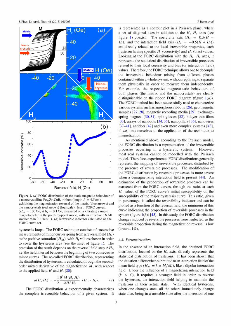
Figure 1. (a) FORC distribution of the static magnetic behaviour ofa nanocrystalline Fe86Zr7CuB6 ribbon (length L = 4.5 cm)exhibiting the magnetization reversal of the matrix (blue arrows) andthe nanocrystals (red arrows) (log scale). Inset: FORC curves.(Hsat = 100 Oe, �Hr = 0.1 Oe, measured on a vibrating samplemagnetometer in the point-by-point mode, with an effective dH/dtsmaller than 0.1 Oe s−1). (b) Reversible indicator calculated on theFORC curve set.

hysteresis loops. The FORC technique consists of successivemeasurements of minor curves going from a reversal field (Hr)

to the positive saturation (Hsat), with Hr values chosen in orderto cover the hysteresis area (see the inset of figure 1). Theprecision of the result depends on the reversal field step �Hr,i.e. the field interval between the beginning of two consecutiveminor curves. The so-called FORC distribution, representingthe distribution of hysterons, is calculated through the second-order mixed derivative of the magnetization M , with respectto the applied field H and Hr [20]:

ρ(H, Hr) = −1

2

∂2M(H, Hr)

∂H∂Hr(H > Hr). (7)

The FORC distribution ρ experimentally characterizesthe complete irreversible behaviour of a given system. It

is represented as a contour plot in a Preisach plane, wherea set of diagonal axes in addition to the H , Hr ones (seefigure 1) coexist. The coercivity axis (Hc = 0.5(H −Hr)) and the interaction field axis (Hu = −0.5(H + Hr))

are directly related to the local irreversible properties, eachhysteron having specific Hc (coercivity) and Hu (bias) values.Looking at the FORC distribution with the Hc, Hu axes, itrepresents the statistical distribution of irreversible processesrelated to their local coercivity and bias (or interaction field)values. Therefore, the FORC technique allows one to decouplethe irreversible behaviour arising from different phasescontained within a whole system, without requiring to separatethem physically in order to measure them independently.For example, the respective magnetostatic behaviours ofboth phases (the matrix and the nanocrystals) are clearlydistinguishable on the ribbon FORC diagram (figure 1(a)).The FORC method has been successfully used to characterizevarious systems such as amorphous ribbons [26], geomagneticsamples [27, 28], magnetic recording media [29], exchange-spring magnets [30, 31], spin glasses [32], bilayer thin films[33], arrays of nanodots [34, 35], nanopillars [36], nanowires[37–41], antidots [42] and even more complex systems [43],if we limit ourselves to the application of the technique tomagnetization.

As mentioned above, according to the Preisach model,the FORC distribution is a representation of the irreversibleprocesses occurring in a hysteretic system. However,most real systems cannot be modelled with the Preisachmodel. Therefore, experimental FORC distributions generallyrepresent the mapping of irreversible processes, disturbed bythe presence of reversible processes. The modification ofthe FORC distribution by reversible processes is more severewhen a demagnetizing interaction field is present [44]. Anestimation of the proportion of reversible processes can beextracted from the FORC curves, through the ratio, at eachHr value, of the FORC curve’s initial susceptibility on thesusceptibility of the major hysteresis curve. This ratio, givenin percentage, is called the reversibility indicator and can beplotted as a function of the reversal field, the minimum of thiscurve indicating the proportion of reversible processes in thesystem (figure 1(b)) [45]. In this study, the FORC distributionchanges induced by reversible processes were neglected, as thereversible proportion during the magnetization reversal is low(around 1%).

3.2. Parametrization

In the absence of an interaction field, the obtained FORCdistribution, located on the Hc axis, directly represents thestatistical distribution of hysterons. It has been shown thatthe situation differs when submitted to an interaction field of themean field type (Hint = k × M/Ms), like a dipolar interactionfield. Under the influence of a magnetizing interaction field(k > 0), it requires a stronger field in order to reversethe hysterons, the interaction field helping to maintain thehysterons in their actual state. With identical hysterons,when one changes state, all the others immediately changestate also, being in a unstable state after the inversion of one

3

J. Phys. D: Appl. Phys. 46 (2013) 045003 F Beron et al

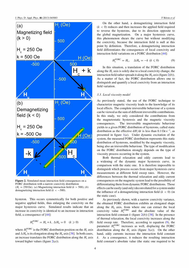
Figure 2. Simulated mean interaction field consequences on aFORC distribution with a narrow coercivity distribution(Hc = 250 Oe). (a) Magnetizing interaction field (k > 500); (b)demagnetizing interaction field (k < −500).

hysteron. This occurs symmetrically for both positive andnegative applied fields, thus enlarging the coercivity on themajor hysteresis curve. Simulated results indicate that anincrease in coercivity is identical to an increase in interactionfield, a consequence of [44]:

H FORCc = Hc + k, �Hu = 0 (k � 0) (8)

where H FORCc is the FORC distribution position on the Hc axis

and �Hu is its elongation along the Hu axis [38]. In both cases,an increase translates the FORC distribution along the Hc axistoward higher values (figure 2(a)).

On the other hand, a demagnetizing interaction field(k < 0) reduces and then increases the applied field requiredto reverse the hysterons, due to its direction opposite tothe global magnetization. On a major hysteresis curve,this phenomenon shears the curve but without modifyingthe coercivity, because the interaction field is null at thispoint by definition. Therefore, a demagnetizing interactionfield differentiates the consequences of local coercivity andinteraction field variations on a FORC distribution [44]:

H FORCc = Hc, �Hu = −k (k � 0) (9)

In this situation, a translation of the FORC distributionalong the Hc axis is solely due to a local coercivity change, theinteraction field rather spreads it along the Hu axis (figure 2(b)).As a matter of fact, the FORC distribution allows one todistinguish and quantify a local coercivity from an interactionfield variation.

3.3. Local viscosity model

As previously stated, the use of the FORC technique tocharacterize magnetic viscosity leads to the knowledge of itslocal effects. The complete irreversible behaviour of a systemcan be viewed as the sum of different irreversible contributions.In this study, we only considered the contributions fromthe magnetostatic hysteresis and the magnetic viscosityconsequences. The irreversible magnetostatic behaviouryields to a given FORC distribution of hysterons, called staticdistribution as the effective dH/dt is less than 0.1 Oe s−1, aspresented in figure 1(a). Under dynamic excitation of thesystem, the measured FORC distribution represents this staticdistribution of hysterons, modified by the magnetic viscosity,being also an irreversible behaviour. The type of modificationon the FORC distribution strongly depends on the type ofviscosity process occurring in the system.

Both thermal relaxation and eddy currents lead toa widening of the dynamic major hysteresis curve, incomparison with the static one. It is therefore impossible todistinguish which process occurs from major hysteresis curvemeasurements at different field sweep rates. However, thedifferences between the thermal relaxation and eddy currentconsequences on the magnetic system lead to the possibility ofdifferentiating them from dynamic FORC distributions. Thoseeffects can be easily (and only) deconvoluted for a system underthe influence of a demagnetizing interaction field (k < 0) (inthe static case).

As previously shown, with a narrow coercivity variance,the obtained FORC distribution exhibits an elongated shapealong the Hu axis, from where one can extract the localcoercivity value H FORC

c and the absolute value of theinteraction field constant k (figure 2(b)) [38]. In the presenceof thermal relaxation, the local coercivity increases along thefield sweep rate. Therefore, according to equation (9), theparameter H FORC

c increases as well, displacing the FORCdistribution along the Hc axis (figure 3(a)). On the otherhand, eddy currents increase the interaction field constantk. As a consequence, it reduces the resulting interactionfield constant’s absolute value (the static one required to be

4

J. Phys. D: Appl. Phys. 46 (2013) 045003 F Beron et al

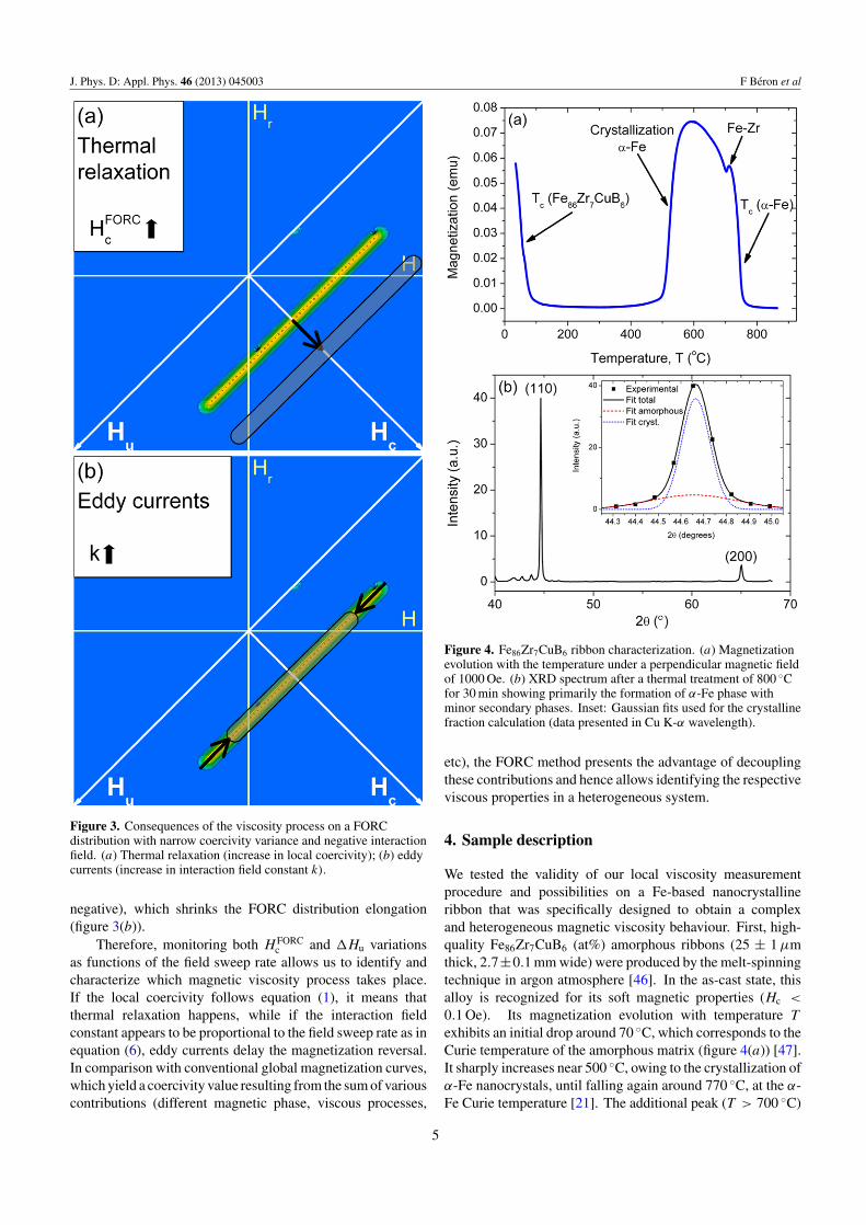
Figure 3. Consequences of the viscosity process on a FORCdistribution with narrow coercivity variance and negative interactionfield. (a) Thermal relaxation (increase in local coercivity); (b) eddycurrents (increase in interaction field constant k).

negative), which shrinks the FORC distribution elongation(figure 3(b)).

Therefore, monitoring both H FORCc and �Hu variations

as functions of the field sweep rate allows us to identify andcharacterize which magnetic viscosity process takes place.If the local coercivity follows equation (1), it means thatthermal relaxation happens, while if the interaction fieldconstant appears to be proportional to the field sweep rate as inequation (6), eddy currents delay the magnetization reversal.In comparison with conventional global magnetization curves,which yield a coercivity value resulting from the sum of variouscontributions (different magnetic phase, viscous processes,

Figure 4. Fe86Zr7CuB6 ribbon characterization. (a) Magnetizationevolution with the temperature under a perpendicular magnetic fieldof 1000 Oe. (b) XRD spectrum after a thermal treatment of 800 ◦Cfor 30 min showing primarily the formation of α-Fe phase withminor secondary phases. Inset: Gaussian fits used for the crystallinefraction calculation (data presented in Cu K-α wavelength).

etc), the FORC method presents the advantage of decouplingthese contributions and hence allows identifying the respectiveviscous properties in a heterogeneous system.

4. Sample description

We tested the validity of our local viscosity measurementprocedure and possibilities on a Fe-based nanocrystallineribbon that was specifically designed to obtain a complexand heterogeneous magnetic viscosity behaviour. First, high-quality Fe86Zr7CuB6 (at%) amorphous ribbons (25 ± 1 µmthick, 2.7±0.1 mm wide) were produced by the melt-spinningtechnique in argon atmosphere [46]. In the as-cast state, thisalloy is recognized for its soft magnetic properties (Hc <

0.1 Oe). Its magnetization evolution with temperature T

exhibits an initial drop around 70 ◦C, which corresponds to theCurie temperature of the amorphous matrix (figure 4(a)) [47].It sharply increases near 500 ◦C, owing to the crystallization ofα-Fe nanocrystals, until falling again around 770 ◦C, at the α-Fe Curie temperature [21]. The additional peak (T > 700 ◦C)

5

J. Phys. D: Appl. Phys. 46 (2013) 045003 F Beron et al

is attributed to secondary crystalline phases, most probablyFe–Zr [48].

The as-cast ribbons underwent a thermal treatment atdifferent temperatures between 400 and 800 ◦C for 30 min.X-ray diffraction (XRD) measurements, performed at theBrazilian National Laboratory of Synchrotron Light Source(LNLS), showed that the α-Fe crystalline fraction increaseslinearly with the thermal treatment temperature, while themean grain diameter steadily increases for T > 600 ◦C [21].In order to create enough pinning sites in the soft amorphousmatrix, we used the system with the highest crystalline fractionfor the subsequent magnetic investigation, that is, treatedat 800 ◦C. XRD measurements showed that the amorphousmatrix represents 30% of the volume of the sample, andthat around 70% of the volume is composed of 70 nm α-Fenanoparticles (figure 4(b)).

The respective static magnetic behaviours of each phaseare indicated on the FORC measurement (figure 1(a) inset) andthe FORC diagram (figure 1(a)). Their quite large coercivity(Hc = 20–35 Oe) suggests that the random anisotropy modelcannot be used in this case. Using the relative heightsbetween the two abrupt magnetization drops observed in themagnetization curves (figure 1(a) inset), the first one wasassociated with the minority phase, i.e. the amorphous matrix,which presents a quasi-reversible behaviour in the absence ofnanocrystals. The magnetization reversal occurs by nucleationpropagation in the matrix after the thermal treatment, wherethe nanocrystals act as pinning sites, enlarging the coercivitydistribution and increasing the mean value. The secondmagnetization drop, which is the most important processin proportion, was identified as from the reversal of α-Fe nanocrystals. Due to the isotropic thermal treatmentapplied, they do not exhibit a preferential anisotropy direction,leading to a large coercivity distribution. A magnetizinginteraction field is generally characterized by a curvature in theFORC distribution, which is slightly shifted towards positiveHu values, and a negative region beneath the distribution[42, 49]. Therefore, both ferromagnetic phases are linked byexchange interaction, which creates a magnetizing interactionfield revealed by the typical ‘corner’ shape of the FORCdistributions (figure 1(a)).

5. Results and discussion

5.1. Viscosity measurements

The dynamic magnetization was acquired with a high-precision ac induction magnetometer working at constantdH/dt [50]. Both major hysteresis curves and FORCmeasurements were performed by varying the dH/dt valuebetween 50 and 6000 Oe s−1 for dynamic characterization. TheFORC measurements cover a ±60 Oe area, with a saturationfield of 100 Oe. Two hundred FORC measurements wereacquired for each dH/dt value, with a precision of �Hr =0.6 Oe. In all cases, the field was applied longitudinally to theaxis of the ribbons. The major hysteresis curve measurementsyield the evolution of the global coercivity value as a functionof the field sweep rate, while the local coercivity variation ofeach distribution was extracted from the FORC measurements.

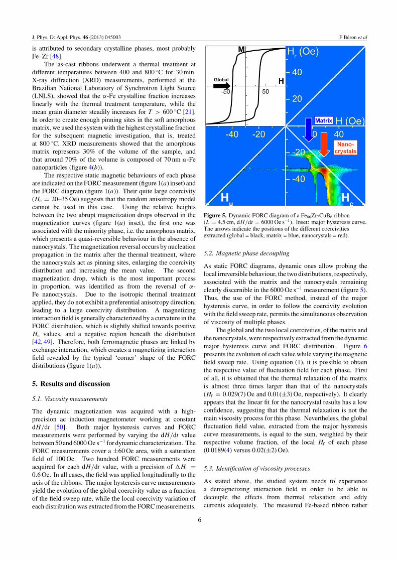
Figure 5. Dynamic FORC diagram of a Fe86Zr7CuB6 ribbon(L = 4.5 cm, dH/dt = 6000 Oe s−1). Inset: major hysteresis curve.The arrows indicate the positions of the different coercivitiesextracted (global = black, matrix = blue, nanocrystals = red).

5.2. Magnetic phase decoupling

As static FORC diagrams, dynamic ones allow probing thelocal irreversible behaviour, the two distributions, respectively,associated with the matrix and the nanocrystals remainingclearly discernible in the 6000 Oe s−1 measurement (figure 5).Thus, the use of the FORC method, instead of the majorhysteresis curve, in order to follow the coercivity evolutionwith the field sweep rate, permits the simultaneous observationof viscosity of multiple phases.

The global and the two local coercivities, of the matrix andthe nanocrystals, were respectively extracted from the dynamicmajor hysteresis curve and FORC distribution. Figure 6presents the evolution of each value while varying the magneticfield sweep rate. Using equation (1), it is possible to obtainthe respective value of fluctuation field for each phase. Firstof all, it is obtained that the thermal relaxation of the matrixis almost three times larger than that of the nanocrystals(Hf = 0.029(7) Oe and 0.01(±3) Oe, respectively). It clearlyappears that the linear fit for the nanocrystal results has a lowconfidence, suggesting that the thermal relaxation is not themain viscosity process for this phase. Nevertheless, the globalfluctuation field value, extracted from the major hysteresiscurve measurements, is equal to the sum, weighted by theirrespective volume fraction, of the local Hf of each phase(0.0189(4) versus 0.02(±2) Oe).

5.3. Identification of viscosity processes

As stated above, the studied system needs to experiencea demagnetizing interaction field in order to be able todecouple the effects from thermal relaxation and eddycurrents adequately. The measured Fe-based ribbon rather

6

J. Phys. D: Appl. Phys. 46 (2013) 045003 F Beron et al

Figure 6. Evolution of the different coercivities with the field sweeprate. The lines are linear fit. A vertical offset was used to distinguishthe curves (L = 4.5 cm).

naturally exhibits a magnetizing interaction field because ofthe exchange interaction between both phases. There aretwo different approaches in order to resolve this problemand to put the system in the proper situation, i.e. with anoverall demagnetizing field: transform the measured data tothe operative plane or experimentally induce a demagnetizingfield.

The usual way consists of calculating an operative fieldHop mimicking the effects of a chosen interaction field ofconstant kop on the measured magnetization M [51]:

Hop = Happl − kopM/Ms. (10)

The FORC distribution is then directly calculated usingHop instead of Happl. Even if the obtained FORC distributionexhibits the expected elongated shape along the Hu axis(figure 7(a)), this method distorts the FORC distribution whenusing a negative kop, i.e. when inducing a demagnetizing field,as in the present case. Because of the high precision requiredto extract accurate data about the local viscosity through theFORC distributions, an alternative way to achieve an overalldemagnetizing field is proposed here.

Instead of mimicking the effects of a demagnetizingfield after the measurement (ex situ), the production ofa demagnetizing field during the measurement (in situ)should lead to undistorted FORC distributions. The easiestexperimental way to achieve this is by reducing the ribbonlength. This way, the shape anisotropy decrease induces astronger demagnetizing field. Using the formulae developedto evaluate the demagnetizing factor of a uniformly magnetizedferromagnetic prism [52] and the theoretical value of Ms forα-Fe (210 emu g−1), we calculated that a ribbon length L of1 cm was similar to applying an external demagnetizing fieldof about 15 Oe along the ribbon. We can see from figure 7(b)that the overall shape of the FORC distribution is similar to theone calculated through the operative field. This procedure iseasily applicable for systems such as ribbons and wires, as longas one takes care of minimizing the consequences of the non-uniformity of the demagnetizing field induced (sample shapeas similar as possible to an ellipsoid of revolution, etc).

Figure 7. Dynamic FORC distribution of a Fe86Zr7CuB6 ribbonobtained with an overall demagnetizing field(dH/dt = 6000 Oe s−1). (a) Calculated translation in the operativeplane (kop = −15 Oe, L = 4.5 cm). (b) Shape demagnetizing fieldinduced experimentally (Hdem ∼ 15 Oe, L = 1 cm).

The obtained FORC diagrams in figure 7 clearly show thepresence of a large coercivity distribution for both the matrixand the nanocrystals, owing to its characteristic wishboneshape (see the appendix). This discrepancy with a narrowFORC distribution, which yields a distribution parallel tothe Hu axis as in figure 3, complicates the quantitativecharacterization of the viscosity processes, but does notinvalidate the conclusions of the local viscosity model.

The second technique was used in order to identify theviscosity process of each phase. The FORC curves weremeasured on the L = 1 cm ribbon, varying dH/dt from 100

7

J. Phys. D: Appl. Phys. 46 (2013) 045003 F Beron et al

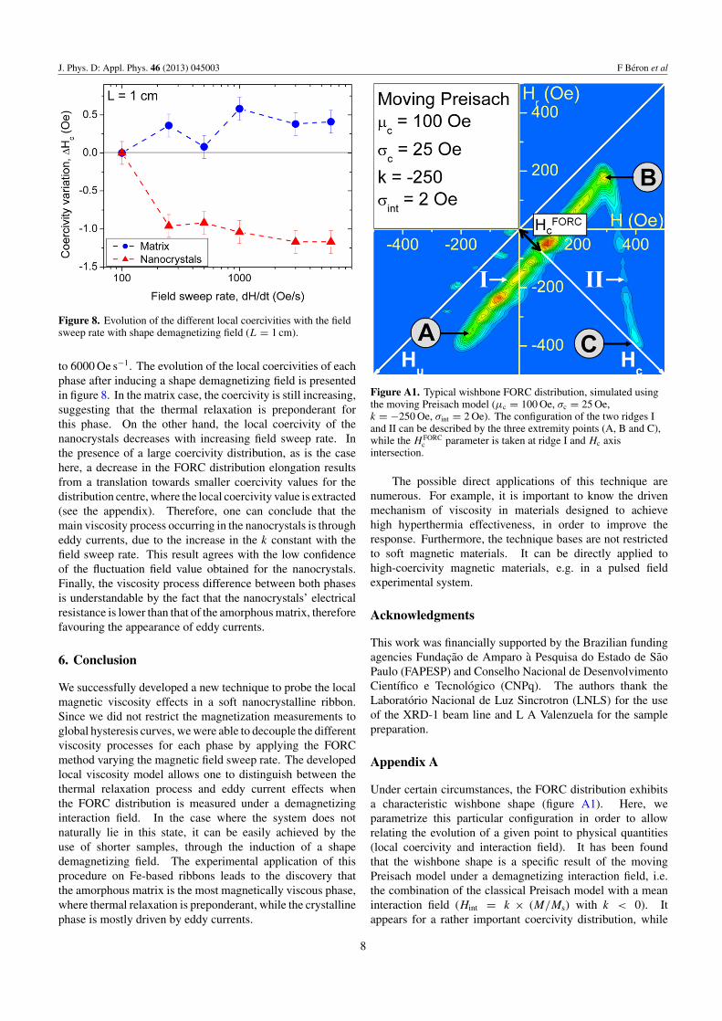
Figure 8. Evolution of the different local coercivities with the fieldsweep rate with shape demagnetizing field (L = 1 cm).

to 6000 Oe s−1. The evolution of the local coercivities of eachphase after inducing a shape demagnetizing field is presentedin figure 8. In the matrix case, the coercivity is still increasing,suggesting that the thermal relaxation is preponderant forthis phase. On the other hand, the local coercivity of thenanocrystals decreases with increasing field sweep rate. Inthe presence of a large coercivity distribution, as is the casehere, a decrease in the FORC distribution elongation resultsfrom a translation towards smaller coercivity values for thedistribution centre, where the local coercivity value is extracted(see the appendix). Therefore, one can conclude that themain viscosity process occurring in the nanocrystals is througheddy currents, due to the increase in the k constant with thefield sweep rate. This result agrees with the low confidenceof the fluctuation field value obtained for the nanocrystals.Finally, the viscosity process difference between both phasesis understandable by the fact that the nanocrystals’ electricalresistance is lower than that of the amorphous matrix, thereforefavouring the appearance of eddy currents.

6. Conclusion

We successfully developed a new technique to probe the localmagnetic viscosity effects in a soft nanocrystalline ribbon.Since we did not restrict the magnetization measurements toglobal hysteresis curves, we were able to decouple the differentviscosity processes for each phase by applying the FORCmethod varying the magnetic field sweep rate. The developedlocal viscosity model allows one to distinguish between thethermal relaxation process and eddy current effects whenthe FORC distribution is measured under a demagnetizinginteraction field. In the case where the system does notnaturally lie in this state, it can be easily achieved by theuse of shorter samples, through the induction of a shapedemagnetizing field. The experimental application of thisprocedure on Fe-based ribbons leads to the discovery thatthe amorphous matrix is the most magnetically viscous phase,where thermal relaxation is preponderant, while the crystallinephase is mostly driven by eddy currents.

Figure A1. Typical wishbone FORC distribution, simulated usingthe moving Preisach model (µc = 100 Oe, σc = 25 Oe,k = −250 Oe, σint = 2 Oe). The configuration of the two ridges Iand II can be described by the three extremity points (A, B and C),while the H FORC

c parameter is taken at ridge I and Hc axisintersection.

The possible direct applications of this technique arenumerous. For example, it is important to know the drivenmechanism of viscosity in materials designed to achievehigh hyperthermia effectiveness, in order to improve theresponse. Furthermore, the technique bases are not restrictedto soft magnetic materials. It can be directly applied tohigh-coercivity magnetic materials, e.g. in a pulsed fieldexperimental system.

Acknowledgments

This work was financially supported by the Brazilian fundingagencies Fundacao de Amparo a Pesquisa do Estado de SaoPaulo (FAPESP) and Conselho Nacional de DesenvolvimentoCientıfico e Tecnologico (CNPq). The authors thank theLaboratorio Nacional de Luz Sincrotron (LNLS) for the useof the XRD-1 beam line and L A Valenzuela for the samplepreparation.

Appendix A

Under certain circumstances, the FORC distribution exhibitsa characteristic wishbone shape (figure A1). Here, weparametrize this particular configuration in order to allowrelating the evolution of a given point to physical quantities(local coercivity and interaction field). It has been foundthat the wishbone shape is a specific result of the movingPreisach model under a demagnetizing interaction field, i.e.the combination of the classical Preisach model with a meaninteraction field (Hint = k × (M/Ms) with k < 0). Itappears for a rather important coercivity distribution, while

8

J. Phys. D: Appl. Phys. 46 (2013) 045003 F Beron et al

the interaction field distribution is kept narrow [38], as for anickel nanopillar array measured along their axes [36].

The wishbone distribution exhibits two distinct ridges,despite the fact that it comes from a unique hysterondistribution. The first one (I), rather narrow along the Hc axiscompared with the result without the interaction field, is notparallel to the Hu axis but slightly tilted counterclockwise. Itis created by the beginning of the switching back of hysterons(passing from the lower to the upper state). Due to the largecoercivity distribution, this reversal starts earlier for positiveHr

values than negative ones because the hysterons with weakercoercivity reverse first (from the upper to the lower state) as thefield is reduced from positive saturation until the reversal field.Therefore, while all hysterons are available to give rise to theFORC distribution at the lower extremity (point A, Hr < 0),only those with the weakest coercivity (denoted as H Low

c ) areavailable at the upper extremity (point B, Hr > 0) [38]. Thesecond ridge (II) simply links the upper limit of I (point B)to the Hc axis (point C). It represents the end of the hysteronswitch back, which does not occur for the same applied fieldvalue because of the coercivity distribution [38].

Using the equations developed in [38], it is possible todescribe the position of points A, B and C in terms of the localcoercivity average µc and standard deviation σc, as well as theinteraction field constant k and standard deviation σint. Therespective Hc and Hu coordinates of ridge I are given by [38]

Hc(I) = HHighc + H Low

c

2(A.1a)

Hu(I) = Hint(Hr) +H

Highc − H Low

c

2(A.1b)

where HHighc and H Low

c represent, respectively, the coercivityof the harder and weaker hysteron that are in their negativestate at Hr, i.e. available to switch back, while Hint(Hr) is thelocal interaction field value at Hr. At point A, all hysteronsare reversed down, as previously explained. The harder andweaker hysterons can therefore be estimated as µc ± 2σc,while the interaction field reaches is maximal value, i.e. −k,leading to

Hc(A) = µc, Hu(A) = −k + 2σc. (A.2)

On the other hand, only a few of the weakest hysterons ofthe system are reversed down at point B, therefore H

Highc =

H Lowc ∼ µc −2σc. The interaction field value is also maximal,

but of opposite direction, k, yielding

Hc(B) = µc − 2σc, Hu(B) = k. (A.3)

The coordinates of point C can be calculated using the ridge IIparametrization:

Hc(II) = H Highc +

Hint(Hr) − Hint(Hsat)

2(A.4a)

Hu(II) = Hint(Hr) + Hint(Hsat)

2(A.4b)

where HHighc ∼ µc + 2σc and the interaction is maximal and

of opposite sign at Hr, where all hysterons are in their lower

state, and at Hsat, where they all switched back. The point Ccoordinates are therefore simply

Hc(C) = µc + 2σc − k, Hu(C) = 0. (A.5)

However, the distribution enlargement arising fromnumerical calculation reduces the localization accuracy ofthese points. The position of ridge I on the Hc axis, H FORC

c ,is simpler to determine with precision. Using equations (A.2)and (A.3) and taking Hu = 0, it yields

H FORCc = µc − 2σc − σck

σc − k. (A.6)

Therefore, the H FORCc parameter characterizing a FORC

distribution with a wishbone shape depends on both the localcoercivity distribution (average and standard deviation) and thelocal interaction field. It is proportional to the local coercivityand reduces in the case where the interaction field constantincreases.

References

[1] Kazantseva N, Hinzke D, Nowak U, Chantrell R W, Atxitia Uand Chubykalo-Fesenko O 2008 Phys. Rev. B 77 184428

[2] Suzuki I S and Suzuki M 2008 Phys. Rev. B 78 214404[3] Anand V K, Adroja D T and Hillier A D 2012 Phys. Rev. B

85 014418[4] Suzuki M, Fullem S I, Suzuki I S, Wang L and Zhong C-J

2009 Phys. Rev. B 79 024418[5] Titov S V, Dejardin P-M, El Mrabti H and Kalmykov Y P 2010

Phys. Rev. B 82 100413(R)[6] de Oliveira L A S, Sinnecker J P, Vieira M D and

Penton-Madrigal A 2010 J. Appl. Phys. 107 09D907[7] Kesserwan H, Manfredi G, Bigot J-Y and Hervieux P A 2011

Phys. Rev. B 84 172407[8] Vittoria C and Yoon S D 2010 Phys. Rev. B 81 014412[9] Sirena M, Steren L B and Guimpel J 2001 Phys. Rev. B

64 104409[10] Wiedenmann A, Gahler R, Dewhurst C D, Keiderling U,

Prevost S and Kohlbrecher J 2011 Phys. Rev. B 84 214303[11] Bertotti G 1991 J. Appl. Phys. 69 4608[12] Street R and Woolley J 1949 Proc. Phys. Soc. Lond. A 62 562[13] Neel L 1950 J. Phys. Radiat. 11 49[14] Labarta A, Iglesias O, Balcells L and Badia F 1993 Phys. Rev.

B 48 10240[15] Gonzalez J M, Montero M I, Vazquez L, Martin Gago J A,

Givord D, de Julian C and O’Grady K 1999 J. Magn. Magn.Mater. 196–197 96

[16] Lyberatos A 1999 J. Magn. Magn. Mater. 191 380[17] Pirota K R, Sartorelli M L, Knobel M, Gutierrez J and

Barandiaran J M 1999 J. Magn. Magn. Mater. 202 431[18] El-Hilo M, O’Grady K and Chantrell R W 2002 J. Magn.

Magn. Mater. 248 360[19] de Oliveira L A S, Sinnecker J P, Grossinger R,

Penton-Madrigal A and Estevez-Rams E 2011 J. Magn.Magn. Mater. 323 1890

[20] Mayergoyz I D 1986 Phys. Rev. Lett. 56 1518[21] Valenzuela L 2011 Amorphous materials characterization

through GMI and GMI-FORC measurements PhD ThesisState University of Campinas

[22] Basso V, Beatrice C, LoBue M, Tiberto P and Bertotti G 2000Phys. Rev. B 61 1278

[23] Wohlfarth E P 1984 J. Phys. F: Met. Phys. 14 L155[24] Adapted from Bertotti G 1998 Hysteresis in Magnetism

(San Diego, CA: Academic)

9

J. Phys. D: Appl. Phys. 46 (2013) 045003 F Beron et al

[25] Preisach F 1935 Z. Phys. 94 277[26] Basso V, Bertotti G, Duhaj P, Ferrara E, Haslar V, Kraus L,

Pokorny J and Zaveta K 1996 J. Magn. Magn. Mater.157/158 217

[27] Roberts A P, Pike C R and Verosub K L 2000 J. Geophys. Res.105 28461

[28] Carvallo C, Muxworthy A R, Dunlop D J and Williams W2003 Earth Planet. Sci. Lett. 213 375

[29] Postolache P, Cerchez M,Stoleriu L and Stancu A 2003 IEEETrans. Magn. 39 2531

[30] Davies J E, Hellwig O, Fullerton E E, Denbeaux G,Kortright J B and Liu K 2004 Phys. Rev. B 70 224434

[31] Chiriac H, Lupu N, Stoleriu L, Postolache P and Stancu A2007 J. Magn. Magn. Mater. 316 177

[32] Katzgraber H G, Pazmandi F, Pike C R, Liu K, Scalettar R T,Verosub K L and Zimanyi G T 2002 Phys. Rev. Lett.89 257202

[33] Navas D et al 2012 New J. Phys. 14 113001[34] Pike C R and Fernandez A 1999 J. Appl. Phys. 85 6668[35] Dumas R K, Li C P, Roshchin I V, Schuller I K and Liu K 2007

Phys. Rev. B 75 134405[36] Pike C R, Ross C A, Scalettar R T and Zimanyi G 2005 Phys.

Rev. B 71 134407[37] Spinu L, Stancu A,Radu C,Li F and Wiley J B 2004 IEEE

Trans. Magn. 40 2116[38] Beron F, Clime L, Ciureanu M, Menard D, Cochrane R W and

Yelon A 2008 J. Nanosci. Nanotechnol. 8 2944[39] Beron F, Carignan L-P, Menard D and Yelon A 2008 IEEE

Trans. Magn. 44 2745

[40] Beron F, Carignan L-P, Menard D and Yelon A 2010Electrodeposited Nanowires and their Applications ed NLupu (Vienna: IN-TECH) pp 167–88

[41] Pirota K R, Beron F, Zanchet D, Rocha T C R, Navas D,Torrejon J, Vazquez M and Knobel M 2011 J. Appl. Phys.109 083919

[42] Beron F, Pirota K R, Vega V, Prida V M, Fernandez A,Hernando B and Knobel M 2011 New J. Phys.13 013035

[43] Beron F, Pirota K R and Knobel M 2012 J. Phys. D: Appl.Phys. 45 505002

[44] Beron F, Menard D and Yelon A 2008 J. Appl. Phys.103 07D908

[45] Beron F, Clime L, Ciureanu M, Cochrane R W, Menard D andYelon A 2007 J. Appl. Phys. 101 09J107

[46] dos Santos D R, Torriani I L, Silva F C S and Knobel M 1999J. Appl. Phys. 86 6993

[47] Gorria P, Orue I, Plazaola F, Fernandez-Gubieda M L andBarandiaran J M 1993 IEEE Trans. Magn. 29 2682

[48] Gomez-Polo C, Holzer D, Multigner M, Navarro E, Agudo P,Hernando A, Vazquez M, Sassik H and Grossinger R 1996Phys. Rev. B 53 3392

[49] Stancu A, Pike C, Stoleriu L, Postolache P and Cimpoesu D2003 J. Appl. Phys. 93 6620

[50] Beron F, Soares G and Pirota K R 2011 Rev. Sci. Instrum.82 063904

[51] Della Torre E and Vajda F 1994 IEEE Trans. Magn.30 4987

[52] Aharoni A 1998 J. Appl. Phys. 83 3432

10