A New Magnetic Sensor Concept for Nondestructive Evaluation of Deteriorated Prestressing Strand

A Thesis

entitled

Magnetic Sensor for Nondestructive Evaluation of Deteriorated Prestressing Strand

by

James D. Wade

Submitted to the Graduate Faculty as partial fulfillment of the requirements for the Master of Science Degree in Civil Engineering

Dr. Douglas Nims, Committee Chair

Dr. Vijay Devabhaktuni, Committee Member Dr. Brian Randolph, Committee Member Dr. Patricia R. Komuniecki, Dean College of Graduate Studies

The University of Toledo May 2010

Copyright 2010, James David Wade

This document is copyrighted material. Under copyright law, no parts of this document may be reproduced without the expressed permission of the author.

iii

An abstract of

Magnetic Sensor for Nondestructive Evaluation of Deteriorated Prestressing Strand

by

James D. Wade

Submitted to the Graduate Faculty in partial fulfillment of the requirements for the Master of Science Degree in Civil Engineering

The University of Toledo

May 2010

The objective of this thesis was to develop a non-destructive in-situ magnetic

technique to investigate the remaining cross-sectional area of prestressing strands.

Corrosion is the predominate failure-mechanism in box-beam bridges. The current

method, visual inspection, is not sufficient as the strands may not be exposed to the

investigator. An inaccurate estimate of the remaining area of strands can lead to an

overestimated strength of the bridge. A new technique involving an electromagnet and

magnetic theories was researched for this thesis.

The experiments conducted have shown that it is possible to distinguish between

different cross-sectional areas using an electromagnet and Hall sensors. Experiments

with an air-gap were first used to simulate concrete cover and provide viability of the

technique. These experiments showed that as the cross-sectional area increased so did

the induced magnetic field.

To further the research, concrete blocks were used in place of the air-gap to better

simulate field conditions. Again, these experiments showed an increase in the induced

magnetic field as the cross-sectional area was increased. Using the data from the air-gap

iv

and concrete block experiments, an approach to determine the cross-sectional area of a

corroded strand under concrete cover was investigated.

v

Acknowlegements

I would like to thank Dr. Douglas Nims for his guidance and engineering

expertise during the production of this research and paper, Dr. Vijay Devabhaktuni and

Bertrand Fernandes for their contributions in establishing the electrical aspect of this

research, and Dr. Brian Randolph for being on the thesis committee and providing

valuable feedback on the research problem and solution. In addition, I would like to

thank the US Department of Transportation for funding this research through the

University of Toledo-University Transportation Research Center and Dr Gottfried

Sawade from the University of Stuttgart, Germany for sharing information about the

electromagnet used in his research. In addition, the design engineers from Ohio

Magnetics, Sophie Zaslavsky and Paul Sheridan were extremely helpful and patient

during the design and procurement process of our final electromagnet. I would also like

to thank MMIStrandCo for their donation of prestressing strand and the Ohio Department

of Transportation for allowing me to hold my presentation at their facility in Bowling

Green, Ohio. Finally, I would like to thank my family for their support and

encouragement throughout the entire process.

vii

Contents

Abstract.......................................................................................................... ............ iii

Acknowledgements.................................................................................................... v

Contents...................................................................................................................... vi

List of Tables.............................................................................................................. ix

List of Figures............................................................................................................. x

1 Introduction.................................................................................................. 1

1.1 Overview............................................................................................ 1

1.2 Problem Statement............................................................................. 2

1.3 Research Objectives........................................................................... 4

1.4 Research Theory and Approach......................................................... 5

2 Literature Review........................................................................................ 9

3 Preliminary Experiments............................................................................ 13

3.1 Background........................................................................................ 13

3.2 Procedure........................................................................................... 14

3.2.1 Trial 1..................................................................................... 15

3.2.2 Trial 2..................................................................................... 16

3.2.3 Trial 3..................................................................................... 16

3.2.4 Trial 4..................................................................................... 18

3.2.5 Trial 5..................................................................................... 19

3.2.6 Trial 6..................................................................................... 20

3.2.7 Trial 7..................................................................................... 21

vii

4 Ohio Magnetics............................................................................................. 24

5 Secondary Experiments............................................................................... 34

5.1 Solid Steel Round Experiments......................................................... 34

5.2 Prestressing Strand Experiments........................................................ 38

5.3 Estimating Cross-Sectional Area Loss............................................... 40

6 Conclusion.................................................................................................... 48

6.1 Results................................................................................................ 48

6.2 Future Research................................................................................. 50

References................................................................................................................. 51

Appendices

Appendix A............................................................................................................... 52

viii

List of Tables

3-1 Trial 1 experimental data.............................................................................. 15







3-8 Brief summary of all trial experiments......................................................... 22

4-1 0.125 inch thick specimen results................................................................. 27

4-2 0.1875 inch thick specimen results............................................................... 28

4-3 0.375 inch thick specimen results................................................................. 28

5-1 Gauss reading for 1018 steel rounds tested at various air-gaps.................... 35

5-2 Gauss reading for 1018 steel rounds tested at various concrete gaps........... 37

5-3 Gauss reading for prestressing strand tested at various air-gaps.................. 39

5-4 Gauss reading for prestressing strands tested at various concrete gaps........ 39

5-5 Results from corroded strand experiments................................................... 43

5-6 Estimates of remaining cross-sectional area of samples 1 and 2 at

115

16" concrete gap......................................................................................... 45

ix

List of Figures

1-1 I-70 collapse.................................................................................................. 2

1-2 I-70 collapse.................................................................................................. 2

1-3 Corroded tendons.......................................................................................... 4

1-4 Hall Effect principle...................................................................................... 6

1-5 Basic block diagram of Hall Effect sensor................................................... 7

3-1 Test equipment set-up................................................................................... 13

3-2 Specimen position for trial 1......................................................................... 14

3-3 Trial 1 area vs. field strength with linear fit equation................................... 15



3-6 Trial 4 area vs. field strength........................................................................ 19



3-9 Trial 7 set-up................................................................................................. 21

3-10 Trial 7 set-up................................................................................................. 21

4-1 Ohio Magnetics test set-up............................................................................ 25

4-2 Air-gap vs. flux density................................................................................. 29

4-3 Area vs. flux density..................................................................................... 29

x

4-4 Flux lines through longitudinal axis of specimen......................................... 31

4-5 Magnetic domain walls................................................................................. 31

4-6 Domain growth curve................................................................................... 32

4-7 Ohio Magnetics electromagnet..................................................................... 33

5-1 Test set-up for 1018 steel rounds with air-gap.............................................. 35

5-2 Gauss reading vs. cross-sectional area for 1018 steel rounds

with air gaps.................................................................................................. 36

5-3 Test set-up for 1018 steel rounds with concrete gap..................................... 37

5-4 Gauss reading vs. cross-sectional area for 1018 steel rounds

with concrete gap.......................................................................................... 38

5-5 Typical prestressing strand section............................................................... 38

5-6 Gauss reading vs. cross-sectional area for prestressing strands

with air-gap................................................................................................... 39

5-7 Gauss reading vs. cross-sectional area for prestressing strands

with concrete gap.......................................................................................... 40

5-8 Test set-up for corroded strand..................................................................... 41

5-9 Separation of wires in corroded strand......................................................... 42

5-10 Example calculation of estimating remaining cross-sectional area.............. 44

5-11 Magnetization curve for iron........................................................................ 47

A-1 Drawing of electromagnet design by Ohio Magnetics................................. 54

1

Chapter 1 Introduction An electromagnet and Hall sensors were used to investigate the remaining cross-sectional

area of prestressing strand due to corrosion.

1.1 Overview

A new non-destructive technique of inspection is needed to evaluate the condition

of prestressing strand in prestressed bridges. The technique studied for this thesis uses an

electromagnet and magnetic theories as an investigation tool. A piece of steel can be

magnetized using an electromagnet and the induced magnetic field can be measured with

a Gauss Meter or other type of Hall sensor equipment. It was hypothesized that a

correlation between the induced magnetic field and cross-sectional area could be

observed. Previous work done state-side and abroad affirmed this hypothesis. There has

been success in Europe in determining fracture locations in prestressed strands using

electromagnetic applications. Researchers in Chicago have been able to detect cross-

sectional area differences of steel rod specimens using electromagnetic applications

(Indacochea). The preliminary experiments described in Chapter 3 of this thesis were the

2

first attempt in proving the magnetic system being investigated in this thesis. The

preliminary experiments were successful in determining cross-sectional area differences.

However, when an air-gap was introduced to simulate concrete cover, the results became

less consistent and a distinction between cross-sectional areas could not be determined

with the initial magnetic system. Due to these observations, future research on this thesis

would include grounding the research with a theoretical basis, as much of the work done

thus far had been a trial and error process. Also, with help from an electromagnet

manufacturer, the design of a stronger magnet needed to magnetize specimens through

the air-gap would be investigated. Finally, once air-gap experiments were successful,

specimens with a concrete block gap were tested.

1.2 Problem Statement

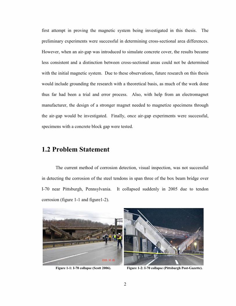
The current method of corrosion detection, visual inspection, was not successful

in detecting the corrosion of the steel tendons in span three of the box beam bridge over

I-70 near Pittsburgh, Pennsylvania. It collapsed suddenly in 2005 due to tendon

corrosion (figure 1-1 and figure1-2).

Figure 1-1: I-70 collapse (Scott 2006). Figure 1-2: I-70 collapse (Pittsburgh Post-Gazette).

3

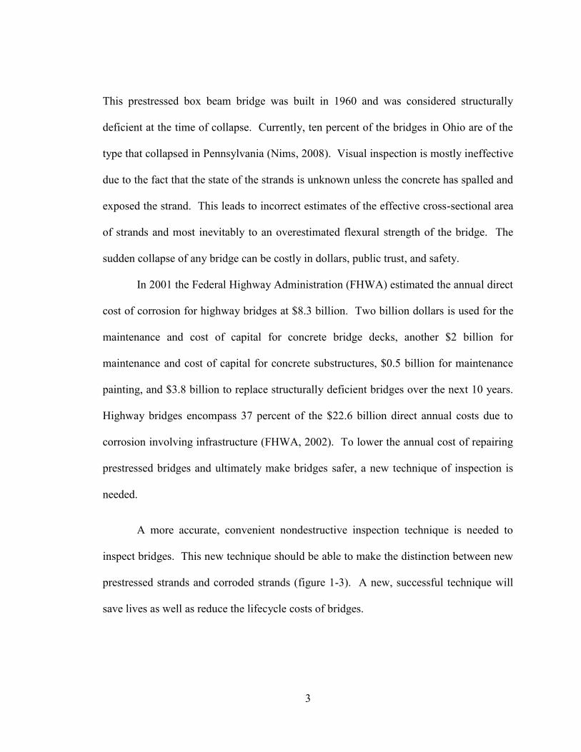
This prestressed box beam bridge was built in 1960 and was considered structurally

deficient at the time of collapse. Currently, ten percent of the bridges in Ohio are of the

type that collapsed in Pennsylvania (Nims, 2008). Visual inspection is mostly ineffective

due to the fact that the state of the strands is unknown unless the concrete has spalled and

exposed the strand. This leads to incorrect estimates of the effective cross-sectional area

of strands and most inevitably to an overestimated flexural strength of the bridge. The

sudden collapse of any bridge can be costly in dollars, public trust, and safety.

In 2001 the Federal Highway Administration (FHWA) estimated the annual direct

cost of corrosion for highway bridges at $8.3 billion. Two billion dollars is used for the

maintenance and cost of capital for concrete bridge decks, another $2 billion for

maintenance and cost of capital for concrete substructures, $0.5 billion for maintenance

painting, and $3.8 billion to replace structurally deficient bridges over the next 10 years.

Highway bridges encompass 37 percent of the $22.6 billion direct annual costs due to

corrosion involving infrastructure (FHWA, 2002). To lower the annual cost of repairing

prestressed bridges and ultimately make bridges safer, a new technique of inspection is

needed.

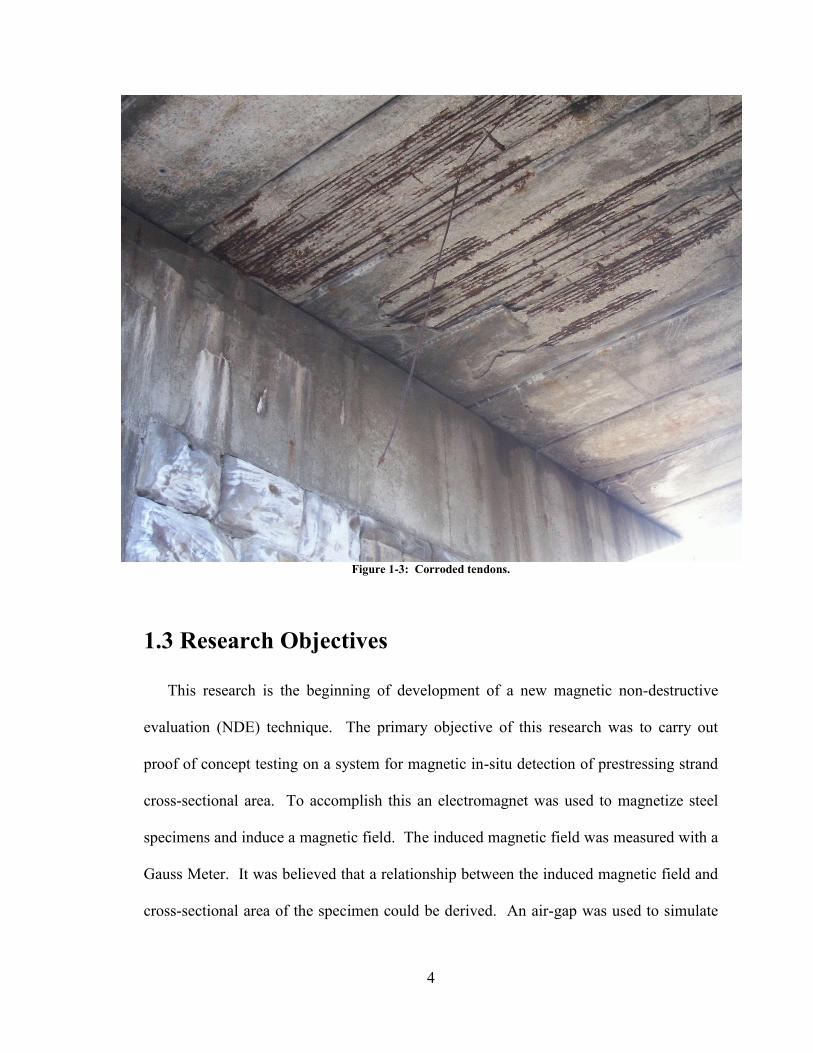
A more accurate, convenient nondestructive inspection technique is needed to

inspect bridges. This new technique should be able to make the distinction between new

prestressed strands and corroded strands (figure 1-3). A new, successful technique will

save lives as well as reduce the lifecycle costs of bridges.

4

Figure 1-3: Corroded tendons.

1.3 Research Objectives

This research is the beginning of development of a new magnetic non-destructive

evaluation (NDE) technique. The primary objective of this research was to carry out

proof of concept testing on a system for magnetic in-situ detection of prestressing strand

cross-sectional area. To accomplish this an electromagnet was used to magnetize steel

specimens and induce a magnetic field. The induced magnetic field was measured with a

Gauss Meter. It was believed that a relationship between the induced magnetic field and

cross-sectional area of the specimen could be derived. An air-gap was used to simulate

5

concrete cover and develop the relationship further. Finally, specimens over concrete

blocks were tested.

1.4 Research Theory and Approach

The magnetic properties of steel are strongly affected by corrosion. Rusting and

corrosion introduce atoms of other elements (typically oxygen) into the material, thus

changing the chemical forms of the material. Due to this change, the steel may become

non-ferromagnetic or less ferromagnetic, thereby, changing the magnetic properties. By

examining the magnetic behavior of steel before and after corrosion, a correlation

between the magnetic properties and loss of steel due to corrosion was made.

In the present approach, the tendons were magnetized by using an electromagnet.

The magnetized tendons had a magnetic field proportional to that of the electromagnet.

The magnetic field strength of the tendons was measured with a Hall Effect sensor, which

provided a voltage reading proportional to the applied magnetic field. Since the magnetic

field strength of the tendon varied with the characteristics of the tendon, such as cross-

sectional area. The present condition of the tendon could be determined through

examination of the magnetic field strength. Examination of the magnetic field strength

required comparison of the newly obtained magnetic field strength to base references

determined in laboratory experiments.

To measure the magnetic field, a Hall Effect sensor was used. A Hall Effect

sensor is a transducer that varies its output voltage in response to changes in the magnetic

field. When a current carrying conductor is placed in the magnetic field, a voltage is

generated perpendicular to both the current and the field. This effect is known as the Hall

6

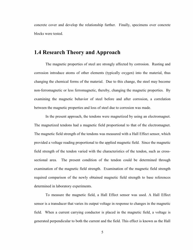
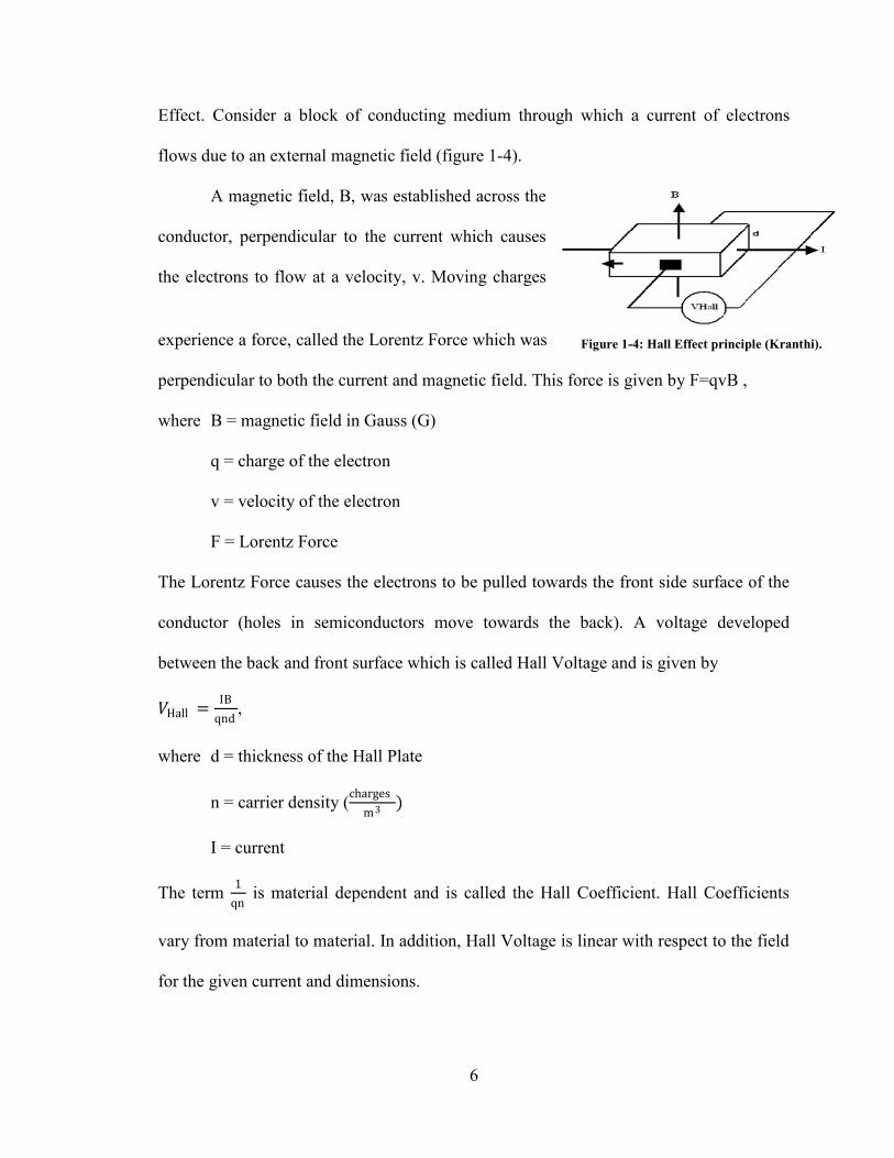
Effect. Consider a block of conducting medium through which a current of electrons

flows due to an external magnetic field (figure 1-4).

A magnetic field, B, was established across the

conductor, perpendicular to the current which causes

the electrons to flow at a velocity, v. Moving charges

experience a force, called the Lorentz Force which was

perpendicular to both the current and magnetic field. This force is given by F=qvB ,

where B = magnetic field in Gauss (G)

q = charge of the electron

v = velocity of the electron

F = Lorentz Force

The Lorentz Force causes the electrons to be pulled towards the front side surface of the

conductor (holes in semiconductors move towards the back). A voltage developed

between the back and front surface which is called Hall Voltage and is given by

𝑉Hall =IB

qnd,

where d = thickness of the Hall Plate

n = carrier density (charges

m3)

I = current

The term 1

qn is material dependent and is called the Hall Coefficient. Hall Coefficients

vary from material to material. In addition, Hall Voltage is linear with respect to the field

for the given current and dimensions.

Figure 1-4: Hall Effect principle (Kranthi).

7

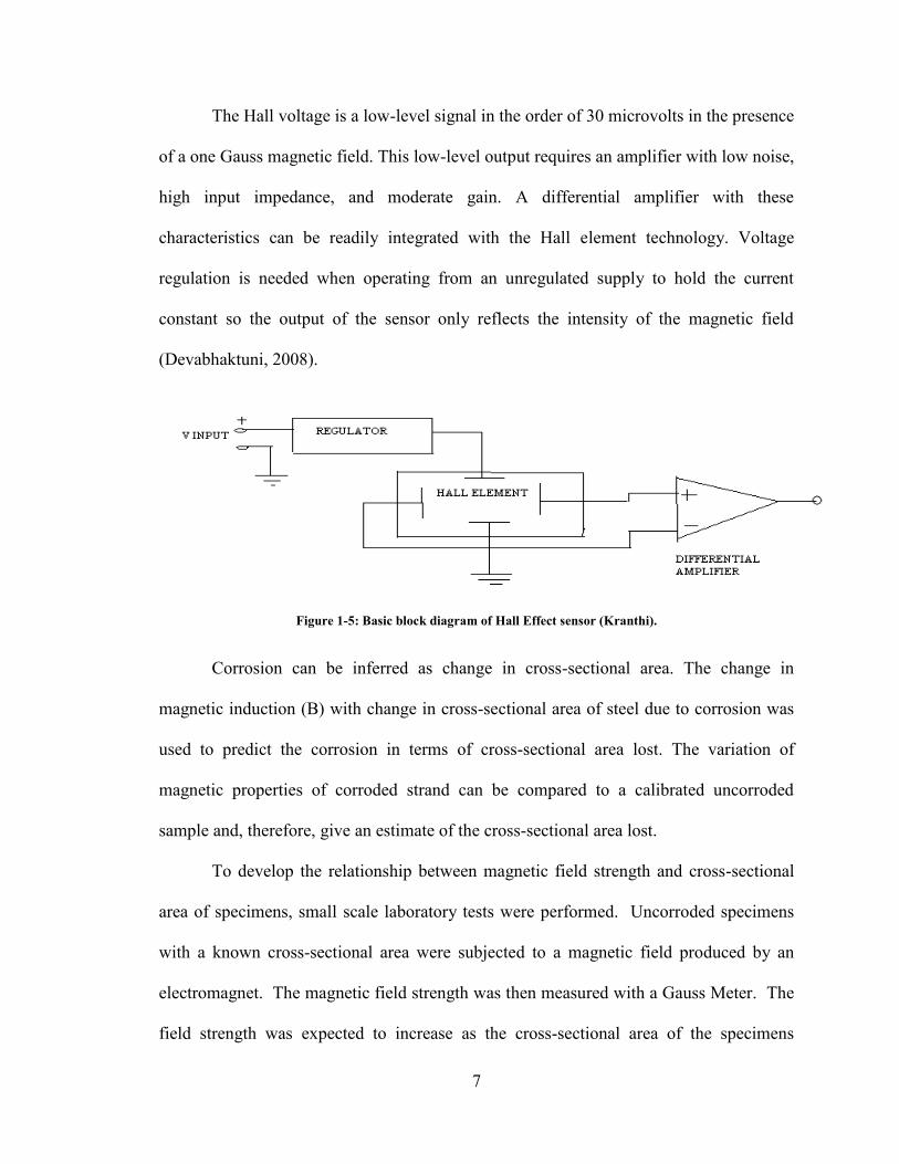
The Hall voltage is a low-level signal in the order of 30 microvolts in the presence

of a one Gauss magnetic field. This low-level output requires an amplifier with low noise,

high input impedance, and moderate gain. A differential amplifier with these

characteristics can be readily integrated with the Hall element technology. Voltage

regulation is needed when operating from an unregulated supply to hold the current

constant so the output of the sensor only reflects the intensity of the magnetic field

(Devabhaktuni, 2008).

Figure 1-5: Basic block diagram of Hall Effect sensor (Kranthi).

Corrosion can be inferred as change in cross-sectional area. The change in

magnetic induction (B) with change in cross-sectional area of steel due to corrosion was

used to predict the corrosion in terms of cross-sectional area lost. The variation of

magnetic properties of corroded strand can be compared to a calibrated uncorroded

sample and, therefore, give an estimate of the cross-sectional area lost.

To develop the relationship between magnetic field strength and cross-sectional

area of specimens, small scale laboratory tests were performed. Uncorroded specimens

with a known cross-sectional area were subjected to a magnetic field produced by an

electromagnet. The magnetic field strength was then measured with a Gauss Meter. The

field strength was expected to increase as the cross-sectional area of the specimens

8

increased. Using this data, a relationship between field strength and cross-sectional area

was developed yielding to an approach that can be used to estimate the remaining sound

cross-sectional area of a corroded strand. Experiments (described in Chapter 3 and 4)

were done in air with an air gap between the specimen and electromagnet. After the

aforementioned experiments were performed successfully, the specimens were placed

over concrete blocks to further simulate field conditions. Finally, corroded specimens

were introduced and subjected to the same testing procedures.

9

Chapter 2

Literature Review

A literature review of existing NDE techniques yielded four popular reoccurring

techniques: ultrasonic defect detection, acoustic emission, ground penetrating radar, and

magnetic flux leakage. The journal article “Evaluation of Corrosion of Prestressing Steel

in Concrete Using Non-destructive Techniques” by Ali and Maddocks published in 2003

gives descriptions of these techniques and several others. A brief description of the four

aforementioned techniques follows:

A. Ultrasonic Defect Detection

A short pulse of ultrasound is generated by means of an electric charge applied to

a piezoelectric crystal which vibrates for a short period at a frequency related to

the crystal thickness. The vibrations rebound to the probe and through ultrasound

equipment and software are converted into an image on a screen. The main

disadvantage of this technique is that it is a passive detection technique rather

than a monitoring technique (Ali, 2003). In addition, only the surface exposed to

the charge is detected rather than the entire volume.

10

B. Acoustic Emission

Acoustic emissions caused by stresses exerted on a material are collected by

transducers that convert mechanical movement into an electrical voltage signal

which can be interpreted as a new crack or other flaw in the material. The main

disadvantage of this technique is that it is a passive detection system that will not

generate data unless an event occurs (Ali, 2003). Corrosion is not a drastic

enough event to register with this type of investigation.

C. Ground Penetrating Radar

An electrically charged pulse signal is transmitted into the material being

examined. Different reflections received represent changing dielectric properties.

The main disadvantage of this technique is that the signal reflects from the surface

nearest the source, thus, information about the cross-sectional area cannot be

obtained (Ali, 2003).

D. Magnetic Flux Leakage Method

A magnetic field is produced by magnetizing the steel tendons. Disturbances or

discontinuities in the magnetic field represent ruptures or reduction of cross-

sectional area. Two significant disadvantages of this technique are that it detects

fractures not loss of area due to corrosion, and it lacks consistency in the

measurement of magnetic fields due to the properties of concrete (Ali, 2003).

The magnetic flux leakage method was studied further by Hillemeier and Scheel.

Their research on this method was published in the journal article “Magnetic Detection of

Prestressing Steel Fractures in Prestressed Concrete” in 1998. Hillemeier and Scheel

used the remnant magnetism method to detect fractures in prestressed concrete structures.

11

They assumed that a magnetized steel wire was comparable to the magnetic field of a bar

magnet. From this, they derived that a signal leakage would be present in the field where

the fracture was present. The tendons were magnetized with a yoke shaped

electromagnet with up to 300 millimeters (12 inches) of concrete cover. The tendons

were magnetized to a saturated state as to eliminate all effects of previous magnetism, i.e.

lifting magnets, electric welding, etc. It was also, discovered that the different properties

of the mild reinforcement and the prestressing steel caused different degrees of

magnetization. As the magnetization increased, prestressing steel was found to increase

towards remanence while the mild reinforcement decreased to lower values. This

allowed for the signals from the prestressing steel to be distinguished from the mild

reinforcement. To simulate fractures in the specimens, the steel wires were cut, flat

ground, and glued. Hall sensors were used to measure the magnetic flux density. Results

showed that fractures could be detected using this method (Hillemeier, 1998).

Rumiche, Indacochea, and Wang also investigated the use of electromagnets to

determine cross-sectional area loss of steel specimens. Their work was published in

“Assessment of the Effect of Microstructure on the Magnetic Behavior of Structural

Carbon Steels Using an Electromagnetic Sensor” in 2007. To simulate cross-sectional

area loss, the specimens were machined down at a two inch region in the middle of the

rod. The specimens were placed within a solenoid electromagnet and magnetized to

saturation. The induced magnetic field was measured by Hall sensors at various positions

along the specimen. They found a linear relationship between the normalized mass loss

and the magnetic saturation for all the samples (Indacochea, 2007).

12

These two aforementioned articles were the basis for much of the work

undertaken in this proposal. The two significant differences being that instead of looking

for fractures like Hillemeier and Scheel, cross-sectional area loss of the strands was the

main objective. The solenoid electromagnet used by Rumiche and his colleagues is a

good method to prove that cross-sectional area can be detected, but this type of magnet

would not be useful in the field as the strands would already be embedded in concrete. A

combination and further exploration of the work described in the above articles lead to a

useful NDE technique for the laboratory and with further research the field.

13

Chapter 3 Preliminary Experiments 3.1 Background

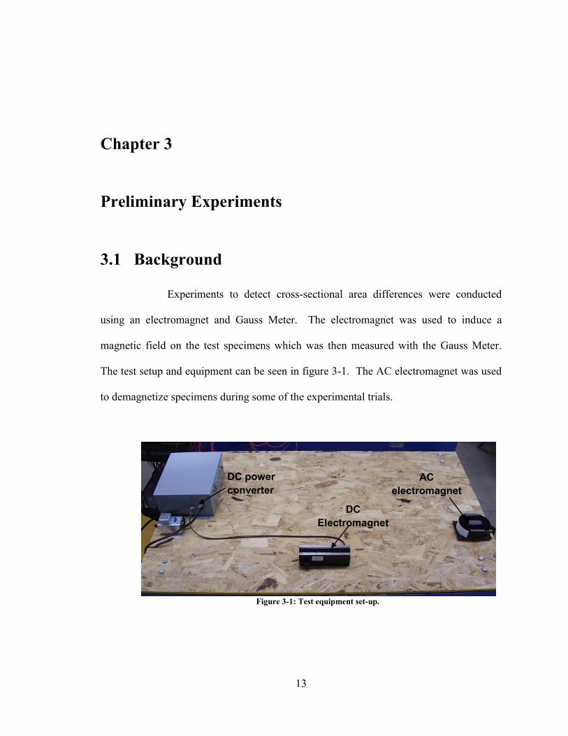
Experiments to detect cross-sectional area differences were conducted

using an electromagnet and Gauss Meter. The electromagnet was used to induce a

magnetic field on the test specimens which was then measured with the Gauss Meter.

The test setup and equipment can be seen in figure 3-1. The AC electromagnet was used

to demagnetize specimens during some of the experimental trials.

Figure 3-1: Test equipment set-up.

DC power converter

DC Electromagnet

AC electromagnet

14

3.2 Procedure

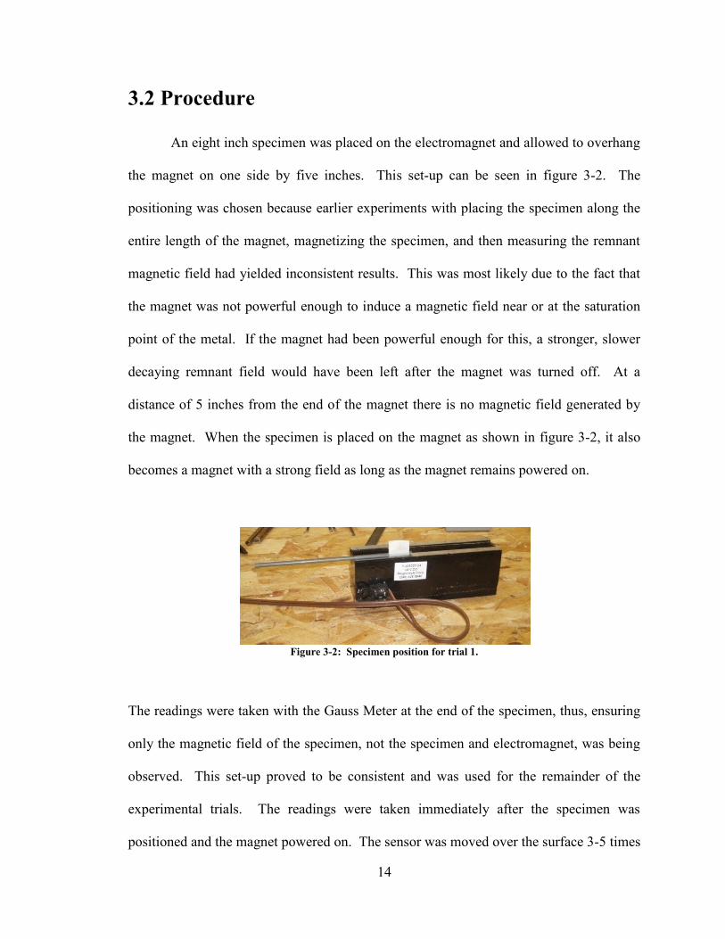
An eight inch specimen was placed on the electromagnet and allowed to overhang

the magnet on one side by five inches. This set-up can be seen in figure 3-2. The

positioning was chosen because earlier experiments with placing the specimen along the

entire length of the magnet, magnetizing the specimen, and then measuring the remnant

magnetic field had yielded inconsistent results. This was most likely due to the fact that

the magnet was not powerful enough to induce a magnetic field near or at the saturation

point of the metal. If the magnet had been powerful enough for this, a stronger, slower

decaying remnant field would have been left after the magnet was turned off. At a

distance of 5 inches from the end of the magnet there is no magnetic field generated by

the magnet. When the specimen is placed on the magnet as shown in figure 3-2, it also

becomes a magnet with a strong field as long as the magnet remains powered on.

Figure 3-2: Specimen position for trial 1.

The readings were taken with the Gauss Meter at the end of the specimen, thus, ensuring

only the magnetic field of the specimen, not the specimen and electromagnet, was being

observed. This set-up proved to be consistent and was used for the remainder of the

experimental trials. The readings were taken immediately after the specimen was

positioned and the magnet powered on. The sensor was moved over the surface 3-5 times

15

and the highest repeatable reading observed was recorded. The specimens underwent

magnetization three times for each trial, and the average field strength was calculated.

This procedure was used for experimental trials 1-6. A description of each trial and the

results of the trial are presented below.

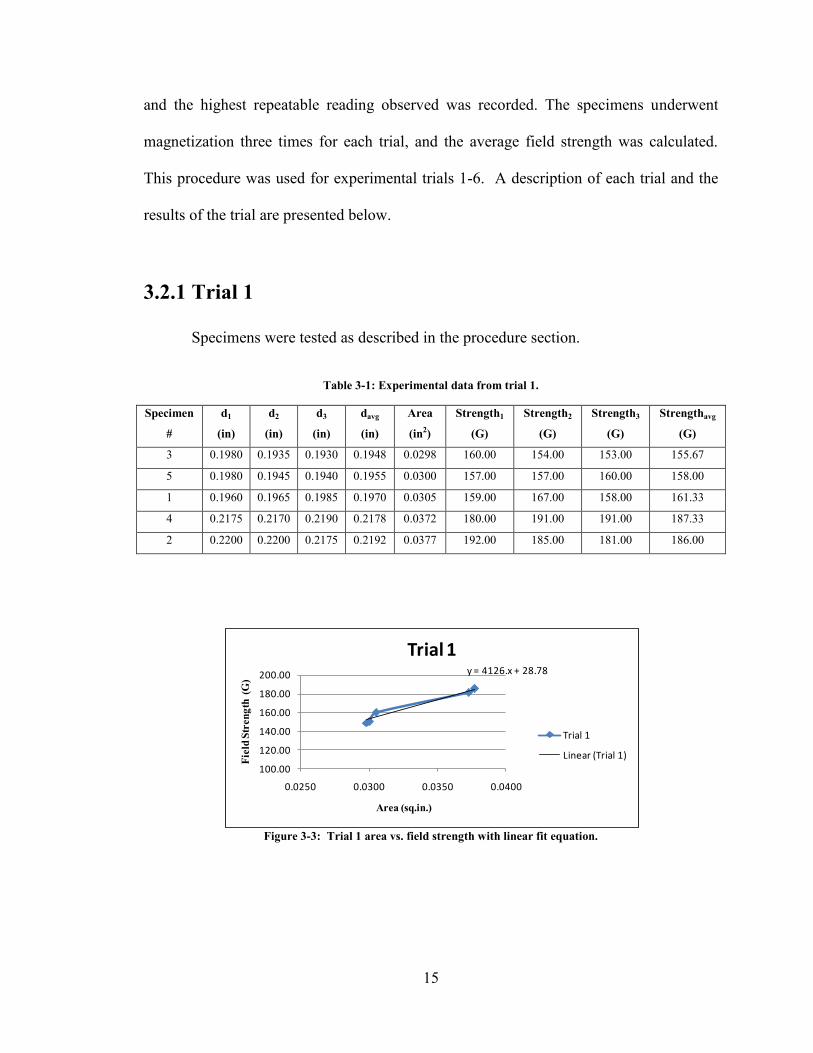
3.2.1 Trial 1

Specimens were tested as described in the procedure section.

Table 3-1: Experimental data from trial 1.

Specimen

#

d1

(in)

d2

(in)

d3

(in)

davg

(in)

Area

(in2)

Strength1

(G)

Strength2

(G)

Strength3

(G)

Strengthavg

(G)

3 0.1980 0.1935 0.1930 0.1948 0.0298 160.00 154.00 153.00 155.67

5 0.1980 0.1945 0.1940 0.1955 0.0300 157.00 157.00 160.00 158.00

1 0.1960 0.1965 0.1985 0.1970 0.0305 159.00 167.00 158.00 161.33

4 0.2175 0.2170 0.2190 0.2178 0.0372 180.00 191.00 191.00 187.33

2 0.2200 0.2200 0.2175 0.2192 0.0377 192.00 185.00 181.00 186.00

Figure 3-3: Trial 1 area vs. field strength with linear fit equation.

y = 4126.x + 28.78

100.00

120.00

140.00

160.00

180.00

200.00

0.0250 0.0300 0.0350 0.0400

Fiel

d St

reng

th (

G)

Area (sq.in.)

Trial 1

Trial 1

Linear (Trial 1)

16

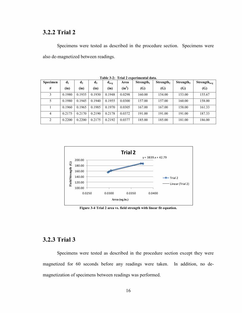
3.2.2 Trial 2

Specimens were tested as described in the procedure section. Specimens were

also de-magnetized between readings.

Table 3-2: Trial 2 experimental data. Specimen

#

d1

(in)

d2

(in)

d3

(in)

davg

(in)

Area

(in2)

Strength1

(G)

Strength2

(G)

Strength3

(G)

Strengthavg

(G)

3 0.1980 0.1935 0.1930 0.1948 0.0298 160.00 154.00 153.00 155.67

5 0.1980 0.1945 0.1940 0.1955 0.0300 157.00 157.00 160.00 158.00

1 0.1960 0.1965 0.1985 0.1970 0.0305 167.00 167.00 158.00 161.33

4 0.2175 0.2170 0.2190 0.2178 0.0372 191.00 191.00 191.00 187.33

2 0.2200 0.2200 0.2175 0.2192 0.0377 185.00 185.00 181.00 186.00

Figure 3-4 Trial 2 area vs. field strength with linear fit equation.

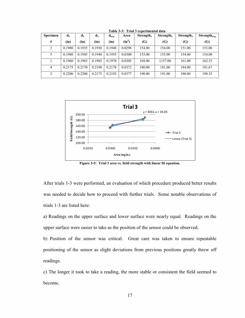
3.2.3 Trial 3

Specimens were tested as described in the procedure section except they were

magnetized for 60 seconds before any readings were taken. In addition, no de-

magnetization of specimens between readings was performed.

y = 3839.x + 42.79

100.00

120.00

140.00

160.00

180.00

200.00

0.0250 0.0300 0.0350 0.0400

Fiel

d St

reng

th (

G)

Area (sq.in.)

Trial 2

Trial 2

Linear (Trial 2)

17

Table 3-3: Trial 3 experimental data Specimen

#

d1

(in)

d2

(in)

d3

(in)

davg

(in)

Area

(in2)

Strength1

(G)

Strength2

(G)

Strength3

(G)

Strengthavg

(G)

3 0.1980 0.1935 0.1930 0.1948 0.0298 154.00 154.00 151.00 153.00

5 0.1980 0.1945 0.1940 0.1955 0.0300 153.00 155.00 154.00 154.00

1 0.1960 0.1965 0.1985 0.1970 0.0305 169.00 1157.00 161.00 162.33

4 0.2175 0.2170 0.2190 0.2178 0.0372 180.00 181.00 184.00 181.67

2 0.2200 0.2200 0.2175 0.2192 0.0377 190.00 191.00 190.00 190.33

Figure 3-5: Trial 3 area vs. field strength with linear fit equation.

After trials 1-3 were performed, an evaluation of which procedure produced better results

was needed to decide how to proceed with further trials. Some notable observations of

trials 1-3 are listed here:

a) Readings on the upper surface and lower surface were nearly equal. Readings on the

upper surface were easier to take as the position of the sensor could be observed.

b) Position of the sensor was critical. Great care was taken to ensure repeatable

positioning of the sensor as slight deviations from previous positions greatly threw off

readings.

c) The longer it took to take a reading, the more stable or consistent the field seemed to

become.

y = 4061.x + 34.05

100.00

120.00

140.00

160.00

180.00

200.00

0.0250 0.0300 0.0350 0.0400

Fiel

d St

reng

th (

G)

Area (sq.in.)

Trial 3

Trial 3

Linear (Trial 3)

18

A timed magnetization may be a good way to get a stable consistent field and

reading. A review of the data collected from trials 1-3 showed that demagnetizing

between readings was not needed. In addition, magnetizing for 60 seconds before taking

a reading seemed to help stabilize the field and led to more consistent results. The

procedures for trial 3 were used for the remainder of the trials unless otherwise noted.

This procedure was chosen because the de-magnetizing seemed to have little or no effect

on the results. Also, the timed magnetization allowed for as many of the dipoles in the

material as possible to become aligned, thus, increasing the induced magnetic field.

The steel used for the specimens in trails 1-3 (specimens 1-5) was cold-rolled

1020 steel. The steel used for trials 4-5 (specimens 6-10) was cold-rolled, but of an

unknown grade. The purpose of trials 4-5 was to use the linear fit equation of trial 3 as a

mathematical means of calculating the field strength. The extrapolated strength was then

compared to the measured strength. Trial 6 used new specimens of the 1020 steel

(specimens 11-15) and these were also used to compare extrapolated magnetic field

strengths to measured field strengths. The data and comparisons for these trials are

shown below.

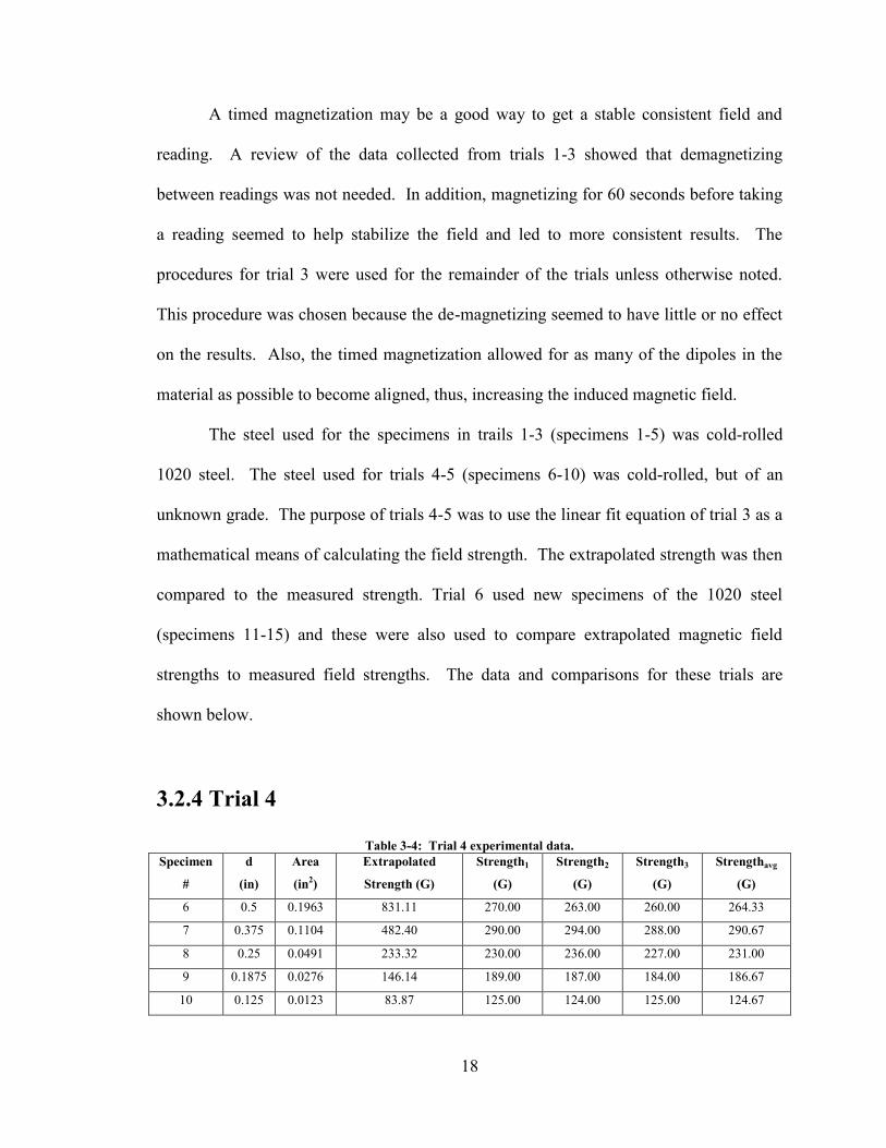
3.2.4 Trial 4


#

d

(in)

Area

(in2)

Extrapolated

Strength (G)

Strength1

(G)

Strength2

(G)

Strength3

(G)

Strengthavg

(G)

6 0.5 0.1963 831.11 270.00 263.00 260.00 264.33

7 0.375 0.1104 482.40 290.00 294.00 288.00 290.67

8 0.25 0.0491 233.32 230.00 236.00 227.00 231.00

9 0.1875 0.0276 146.14 189.00 187.00 184.00 186.67

10 0.125 0.0123 83.87 125.00 124.00 125.00 124.67

19

Figure 3-6: Trial 4 area vs. field strength.

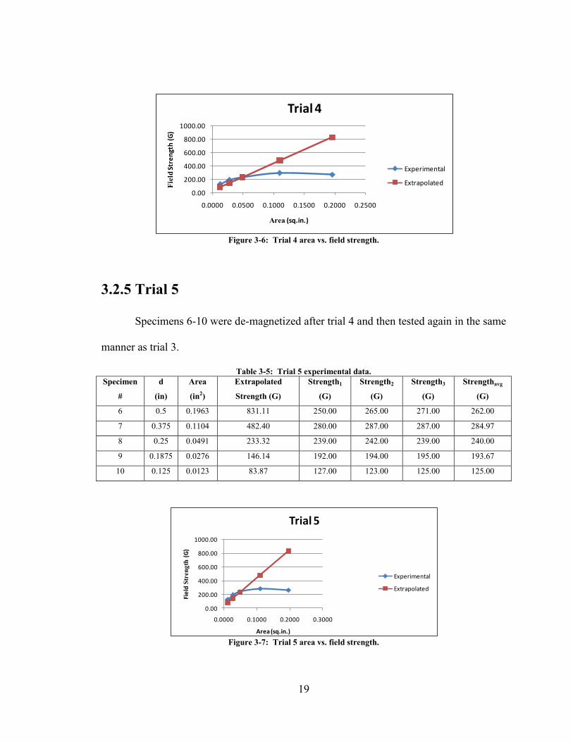
3.2.5 Trial 5

Specimens 6-10 were de-magnetized after trial 4 and then tested again in the same

manner as trial 3.


#

d

(in)

Area

(in2)

Extrapolated

Strength (G)

Strength1

(G)

Strength2

(G)

Strength3

(G)

Strengthavg

(G)

6 0.5 0.1963 831.11 250.00 265.00 271.00 262.00

7 0.375 0.1104 482.40 280.00 287.00 287.00 284.97

8 0.25 0.0491 233.32 239.00 242.00 239.00 240.00

9 0.1875 0.0276 146.14 192.00 194.00 195.00 193.67

10 0.125 0.0123 83.87 127.00 123.00 125.00 125.00


0.00

200.00

400.00

600.00

800.00

1000.00

0.0000 0.0500 0.1000 0.1500 0.2000 0.2500

Fiel

dSt

ren

gth

(G

)

Area (sq.in.)

Trial 4

Experimental

Extrapolated

0.00

200.00

400.00

600.00

800.00

1000.00

0.0000 0.1000 0.2000 0.3000

Fie

ld S

tren

gth

(G)

Area (sq.in.)

Trial 5

Experimental

Extrapolated

20

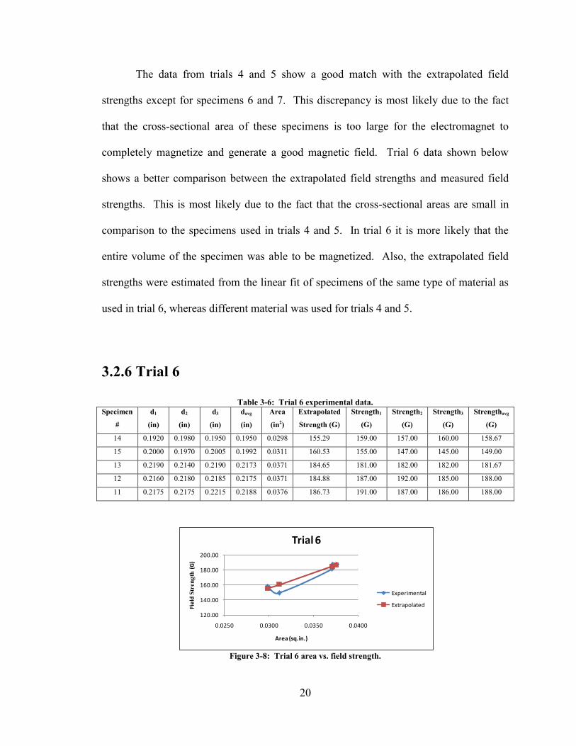
The data from trials 4 and 5 show a good match with the extrapolated field

strengths except for specimens 6 and 7. This discrepancy is most likely due to the fact

that the cross-sectional area of these specimens is too large for the electromagnet to

completely magnetize and generate a good magnetic field. Trial 6 data shown below

shows a better comparison between the extrapolated field strengths and measured field

strengths. This is most likely due to the fact that the cross-sectional areas are small in

comparison to the specimens used in trials 4 and 5. In trial 6 it is more likely that the

entire volume of the specimen was able to be magnetized. Also, the extrapolated field

strengths were estimated from the linear fit of specimens of the same type of material as

used in trial 6, whereas different material was used for trials 4 and 5.

3.2.6 Trial 6


#

d1

(in)

d2

(in)

d3

(in)

davg

(in)

Area

(in2)

Extrapolated

Strength (G)

Strength1

(G)

Strength2

(G)

Strength3

(G)

Strengthavg

(G)

14 0.1920 0.1980 0.1950 0.1950 0.0298 155.29 159.00 157.00 160.00 158.67

15 0.2000 0.1970 0.2005 0.1992 0.0311 160.53 155.00 147.00 145.00 149.00

13 0.2190 0.2140 0.2190 0.2173 0.0371 184.65 181.00 182.00 182.00 181.67

12 0.2160 0.2180 0.2185 0.2175 0.0371 184.88 187.00 192.00 185.00 188.00

11 0.2175 0.2175 0.2215 0.2188 0.0376 186.73 191.00 187.00 186.00 188.00


120.00

140.00

160.00

180.00

200.00

0.0250 0.0300 0.0350 0.0400

Fie

ld S

tren

gth

(G)

Area (sq.in.)

Trial 6

Experimental

Extrapolated

21

In addition to these trials, trials with concrete reinforcing bar specimens were

performed. The data collected consistently showed that a higher cross-sectional area

yielded a higher magnetic field strength. However, the readings of the field strength

varied a considerable amount. This is most likely due to the ribs in the rebar. If the

sensor was placed on a rib for a reading, the reading observed was much higher than if it

were placed on a smooth spot on the bar. In later work, this was resolved by mounting

the sensor on the pole face.

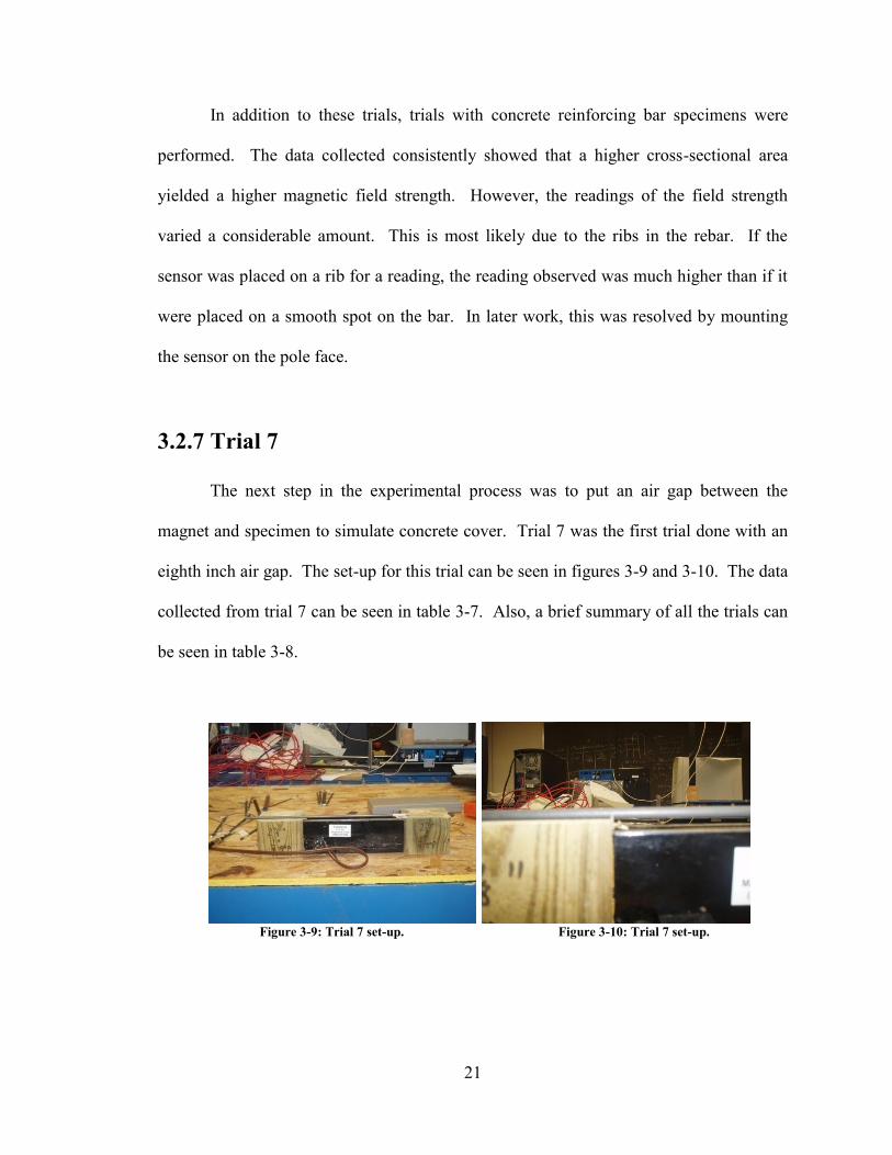
3.2.7 Trial 7

The next step in the experimental process was to put an air gap between the

magnet and specimen to simulate concrete cover. Trial 7 was the first trial done with an

eighth inch air gap. The set-up for this trial can be seen in figures 3-9 and 3-10. The data

collected from trial 7 can be seen in table 3-7. Also, a brief summary of all the trials can

be seen in table 3-8.

Figure 3-9: Trial 7 set-up. Figure 3-10: Trial 7 set-up.

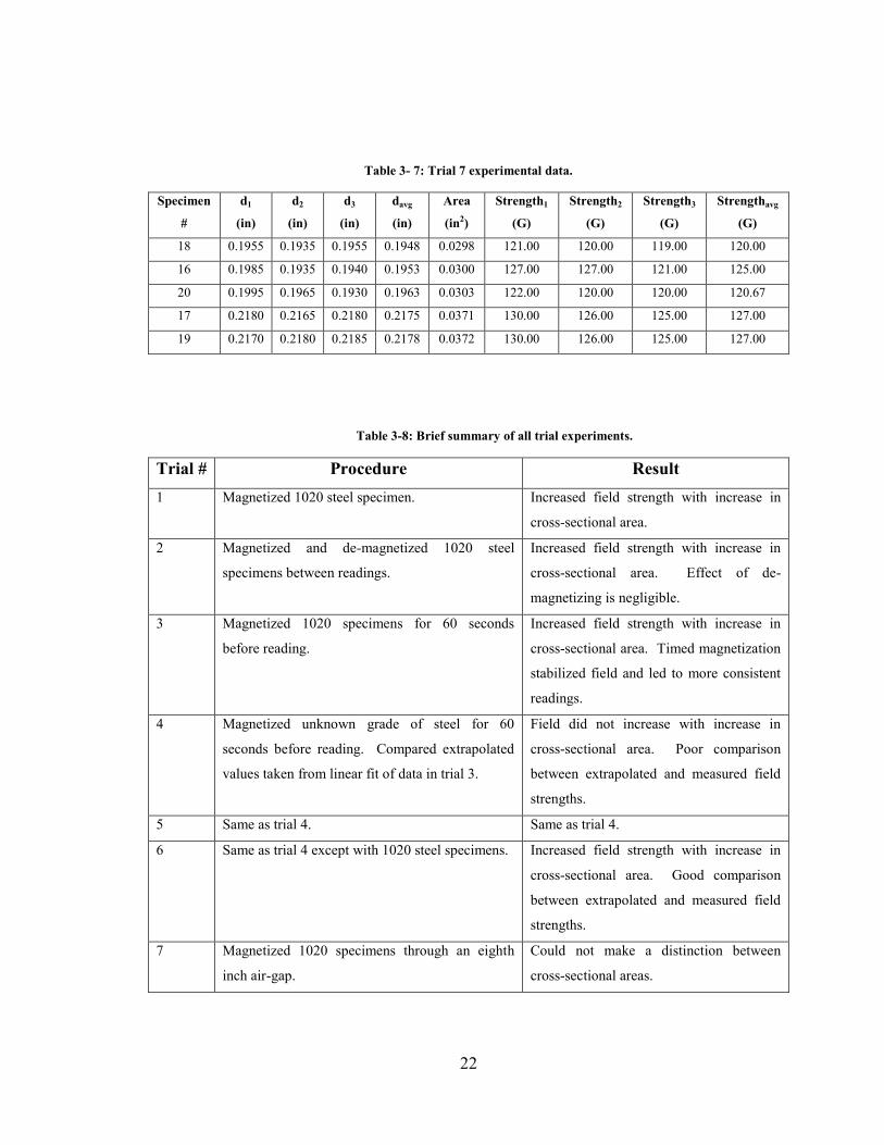
22

Table 3- 7: Trial 7 experimental data.

Specimen

#

d1

(in)

d2

(in)

d3

(in)

davg

(in)

Area

(in2)

Strength1

(G)

Strength2

(G)

Strength3

(G)

Strengthavg

(G)

18 0.1955 0.1935 0.1955 0.1948 0.0298 121.00 120.00 119.00 120.00

16 0.1985 0.1935 0.1940 0.1953 0.0300 127.00 127.00 121.00 125.00

20 0.1995 0.1965 0.1930 0.1963 0.0303 122.00 120.00 120.00 120.67

17 0.2180 0.2165 0.2180 0.2175 0.0371 130.00 126.00 125.00 127.00

19 0.2170 0.2180 0.2185 0.2178 0.0372 130.00 126.00 125.00 127.00

Table 3-8: Brief summary of all trial experiments.

Trial # Procedure Result 1 Magnetized 1020 steel specimen. Increased field strength with increase in

cross-sectional area.

2 Magnetized and de-magnetized 1020 steel

specimens between readings.

Increased field strength with increase in

cross-sectional area. Effect of de-

magnetizing is negligible.

3 Magnetized 1020 specimens for 60 seconds

before reading.

Increased field strength with increase in

cross-sectional area. Timed magnetization

stabilized field and led to more consistent

readings.

4 Magnetized unknown grade of steel for 60

seconds before reading. Compared extrapolated

values taken from linear fit of data in trial 3.

Field did not increase with increase in

cross-sectional area. Poor comparison

between extrapolated and measured field

strengths.

5 Same as trial 4. Same as trial 4.

6 Same as trial 4 except with 1020 steel specimens. Increased field strength with increase in

cross-sectional area. Good comparison

between extrapolated and measured field

strengths.

7 Magnetized 1020 specimens through an eighth

inch air-gap.

Could not make a distinction between

cross-sectional areas.

23

A review of the data reveals that the field strength did not necessarily increase

with cross-sectional area. This is due to the limitation of the electromagnet being used.

The electromagnet is not strong enough to induce a strong field in specimens that are not

in direct contact with its surface or that have a large cross-sectional area such as

specimens 6 and 7. The preliminary experiments thus far have been a trial and error

process. However this process led to some interesting findings, most notably, that there

is a relationship between field strength and cross-sectional area. It appears from these

experiments that the electromagnet being used is not adequate to induce a magnetic field

in the specimen when an air-gap is introduced.

24

Chapter 4 Ohio Magnetics

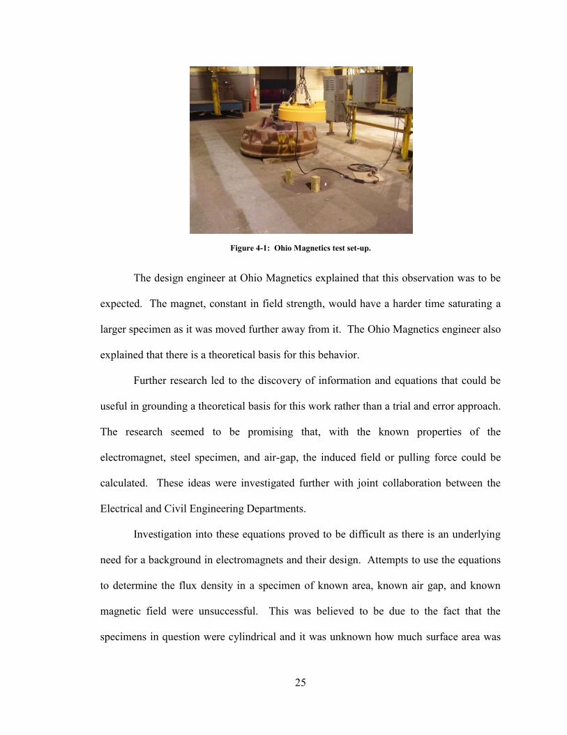
To develop a magnet capable of inducing a strong magnetic field in

prestressing strands covered in two inches of concrete a commercial electromagnet

manufacturer was contacted. Ohio Magnetics specializes in the design and production of

commercial magnets used in salvage yards and recycling facilities. A twenty-five inch

diameter POW-R-LITE magnet was used at their facility to investigate if a larger magnet

would help with getting more accurate and consistent readings when an air gap was

introduced. The magnet and test set-up can be seen in figure 4-1. The air gap tested with

this magnet was 2.875 inches which is beyond what would be seen in the field. The test

set-up was not known until arrival at the facility, and proper action could not be taken to

ensure a proper, more adequate air gap. However, at this air gap, the specimens were

able to be magnetized, but the results were opposite of what was expected. Instead of the

reading increasing as the area of the specimen increased, a decrease in the flux density

reading was observed.

25

Figure 4-1: Ohio Magnetics test set-up.

The design engineer at Ohio Magnetics explained that this observation was to be

expected. The magnet, constant in field strength, would have a harder time saturating a

larger specimen as it was moved further away from it. The Ohio Magnetics engineer also

explained that there is a theoretical basis for this behavior.

Further research led to the discovery of information and equations that could be

useful in grounding a theoretical basis for this work rather than a trial and error approach.

The research seemed to be promising that, with the known properties of the

electromagnet, steel specimen, and air-gap, the induced field or pulling force could be

calculated. These ideas were investigated further with joint collaboration between the

Electrical and Civil Engineering Departments.

Investigation into these equations proved to be difficult as there is an underlying

need for a background in electromagnets and their design. Attempts to use the equations

to determine the flux density in a specimen of known area, known air gap, and known

magnetic field were unsuccessful. This was believed to be due to the fact that the

specimens in question were cylindrical and it was unknown how much surface area was

26

exposed to the magnetic flux lines of the magnet, and also because only one yoke of the

magnet was being utilized. To further investigate this matter, it was decided to try the

equations with a flat specimen that would utilize both yokes in their entirety.

The use of a flat specimen in the equations was also unsuccessful. The results

obtained were not consistent or what was expected. From these investigations, two

conclusions were drawn about the use of these equations for our applications. First, the

equations were derived for a toroid shaped magnet; thus, possibly causing them to need

adjustments for a rectangular type magnet. Further, the air gap used for the derivation of

the equations refers to a small slit in the circular shape which creates a defined north and

south pole in the magnet. This change in the magnet causes the flux lines to flow from

one pole to the other, hence, the air gap is uniformly magnetized. Our application calls

for an air gap to be introduced not within the magnetic circuit, but externally. In our

application, the electromagnet yokes remain as a closed magnetic circuit and another

magnetic circuit is added by the application of the steel specimens; thus, the air gap

distance becomes crucial as the flux lines produced by the magnet are constant. The

reluctance of the air gap itself and the specimen also play a crucial role. Air has a high

reluctance to magnetic fields, so much of the energy is dissipated before reaching the

specimen. Secondly, it could very well be that our limited exposure to electromagnets

and their design has hindered our attempts to successfully use the equations. It may be

that we are just using the equations incorrectly or are making incorrect assumptions. If

this is the case, we have no way of checking ourselves since this a unique project with

ideas that have only been attempted by a few others. After these investigations and an

27

analysis of the results, it was decided to proceed on the assumption that the equations

were not suitable for our application.

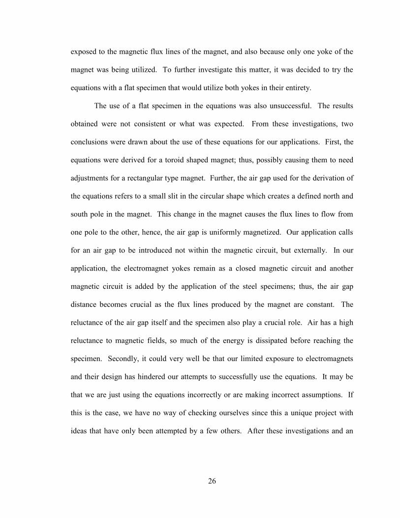
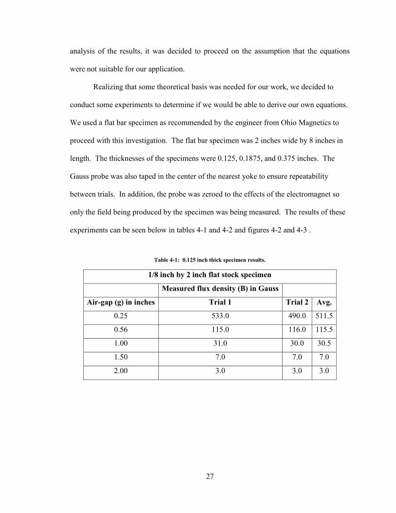
Realizing that some theoretical basis was needed for our work, we decided to

conduct some experiments to determine if we would be able to derive our own equations.

We used a flat bar specimen as recommended by the engineer from Ohio Magnetics to

proceed with this investigation. The flat bar specimen was 2 inches wide by 8 inches in

length. The thicknesses of the specimens were 0.125, 0.1875, and 0.375 inches. The

Gauss probe was also taped in the center of the nearest yoke to ensure repeatability

between trials. In addition, the probe was zeroed to the effects of the electromagnet so

only the field being produced by the specimen was being measured. The results of these

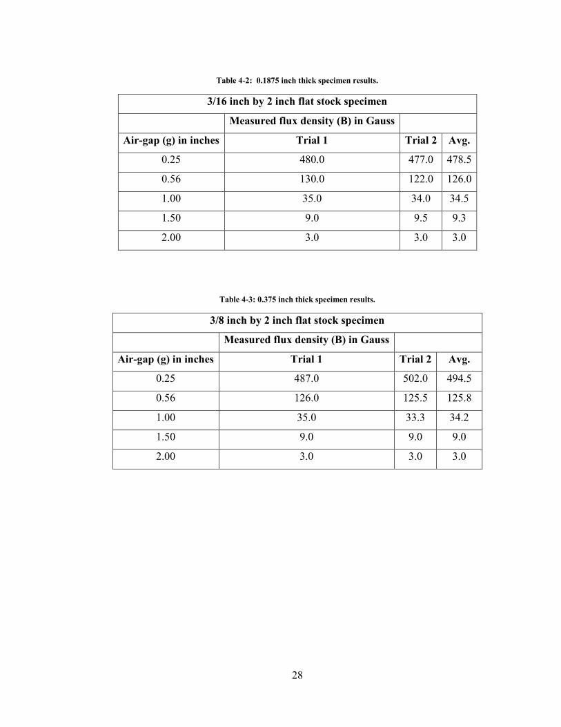
experiments can be seen below in tables 4-1 and 4-2 and figures 4-2 and 4-3 .

Table 4-1: 0.125 inch thick specimen results.

1/8 inch by 2 inch flat stock specimen

Measured flux density (B) in Gauss

Air-gap (g) in inches Trial 1 Trial 2 Avg.

0.25 533.0 490.0 511.5

0.56 115.0 116.0 115.5

1.00 31.0 30.0 30.5

1.50 7.0 7.0 7.0

2.00 3.0 3.0 3.0

28





0.25 480.0 477.0 478.5

0.56 130.0 122.0 126.0

1.00 35.0 34.0 34.5

1.50 9.0 9.5 9.3

2.00 3.0 3.0 3.0





0.25 487.0 502.0 494.5

0.56 126.0 125.5 125.8

1.00 35.0 33.3 34.2

1.50 9.0 9.0 9.0

2.00 3.0 3.0 3.0

29

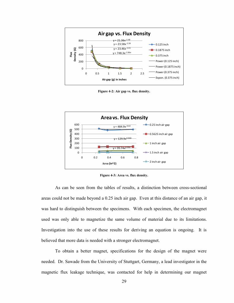
Figure 4-2: Air gap vs. flux density.

Figure 4-3: Area vs. flux density.

As can be seen from the tables of results, a distinction between cross-sectional

areas could not be made beyond a 0.25 inch air gap. Even at this distance of an air gap, it

was hard to distinguish between the specimens. With each specimen, the electromagnet

used was only able to magnetize the same volume of material due to its limitations.

Investigation into the use of these results for deriving an equation is ongoing. It is

believed that more data is needed with a stronger electromagnet.

To obtain a better magnet, specifications for the design of the magnet were

needed. Dr. Sawade from the University of Stuttgart, Germany, a lead investigator in the

magnetic flux leakage technique, was contacted for help in determining our magnet

y = 21.36x-2.48

y = 23.58x-2.39

y = 23.46x-2.41

y = 748.3e-2.86x

0

200

400

600

800

0 0.5 1 1.5 2 2.5Fl

ux

De

nsi

ty (

G)

Air gap (g) in inches

Air gap vs. Flux Density

0.125 inch

0.1875 inch

0.375 inch

Power (0.125 inch)

Power (0.1875 inch)

Power (0.375 inch)

Expon. (0.375 inch)

y = 484.9x-0.02

y = 129.9x0.068

y = 35.74x0.090

0

100

200

300

400

500

600

0 0.2 0.4 0.6 0.8

Flu

x D

en

sity

(G

)

Area (in^2)

Area vs. Flux Density0.25 inch air gap

0.5625 inch air gap

1 inch air gap

1.5 inch air gap

2 inch air gap

30

specifications. The magnet specifications we decided to use are the same used in

Germany for MLF as they have been successful in magnetizing specimens under several

inches of concrete. The magnetization should be by an electrically excited yoke (length

about 8 to 16 in.). The magnetic field should reach up to 381-508 Ampre

in . with the axial

component in the middle of the yoke. A gap of 8 in or less between working poles would

be acceptable. The field should also be adjustable through an autotransformer

arrangement.

These specifications were emailed to 3 different manufacturers to determine if

any of them had this or a similar magnet in stock (Ohio Magnetics, Magnetool,

Magnetechcorp). Ohio Magnetics was the manufacturer chosen to complete the design

and construction of the magnet. The first magnet design purposed by Ohio Magnetics

exceeded the criteria set-forth, but further investigation into the design led to a

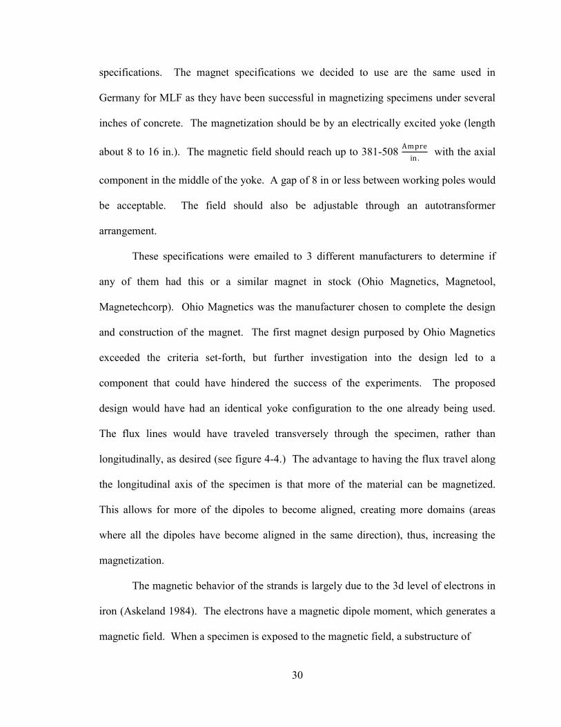
component that could have hindered the success of the experiments. The proposed

design would have had an identical yoke configuration to the one already being used.

The flux lines would have traveled transversely through the specimen, rather than

longitudinally, as desired (see figure 4-4.) The advantage to having the flux travel along

the longitudinal axis of the specimen is that more of the material can be magnetized.

This allows for more of the dipoles to become aligned, creating more domains (areas

where all the dipoles have become aligned in the same direction), thus, increasing the

magnetization.

The magnetic behavior of the strands is largely due to the 3d level of electrons in

iron (Askeland 1984). The electrons have a magnetic dipole moment, which generates a

magnetic field. When a specimen is exposed to the magnetic field, a substructure of

31

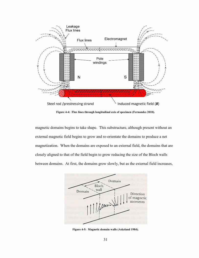
Figure 4-4: Flux lines through longitudinal axis of specimen (Fernandes 2010).

magnetic domains begins to take shape. This substructure, although present without an

external magnetic field begins to grow and re-orientate the domains to produce a net

magnetization. When the domains are exposed to an external field, the domains that are

closely aligned to that of the field begin to grow reducing the size of the Bloch walls

between domains. At first, the domains grow slowly, but as the external field increases,

Figure 4-5: Magnetic domain walls (Askeland 1984).

32

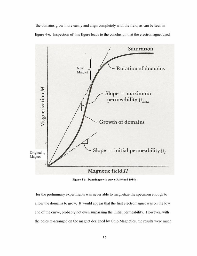
the domains grow more easily and align completely with the field, as can be seen in

figure 4-6. Inspection of this figure leads to the conclusion that the electromagnet used

Figure 4-6: Domain growth curve (Askeland 1984).

for the preliminary experiments was never able to magnetize the specimen enough to

allow the domains to grow. It would appear that the first electromagnet was on the low

end of the curve, probably not even surpassing the initial permeability. However, with

the poles re-arranged on the magnet designed by Ohio Magnetics, the results were much

Original Magnet

m

New Magnet

m

33

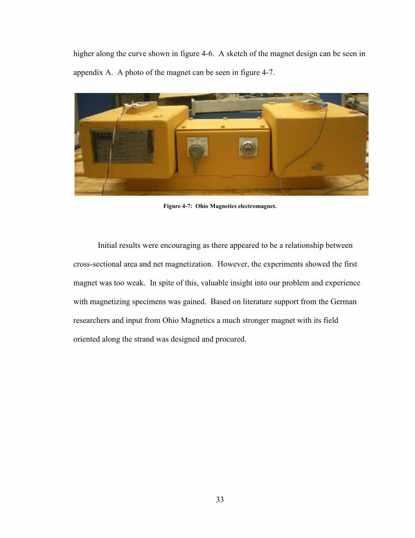
higher along the curve shown in figure 4-6. A sketch of the magnet design can be seen in

appendix A. A photo of the magnet can be seen in figure 4-7.

Figure 4-7: Ohio Magnetics electromagnet.

Initial results were encouraging as there appeared to be a relationship between

cross-sectional area and net magnetization. However, the experiments showed the first

magnet was too weak. In spite of this, valuable insight into our problem and experience

with magnetizing specimens was gained. Based on literature support from the German

researchers and input from Ohio Magnetics a much stronger magnet with its field

oriented along the strand was designed and procured.

34

Chapter 5 Experiments With Strong Magnet

Along with a new magnet, new testing procedures were adopted. When testing

the magnet at the Ohio Magnetics facility before acceptance of the product, the engineers

had decided to measure the induced field by placing the sensor on the pole face rather

than on the specimen. This was advantageous for two reasons: 1) It would eliminate

errors due to inconsistency in sensor placement along the specimen. 2) It was more field

applicable as the sensor could not be placed along a stand embedded in concrete.

5.1 Solid Steel Round Experiments

Other than the aforementioned changes, the testing with the new magnet was

similar to those used in the preliminary experiments. The readings for all experiments

discussed from this point forward were taken from the right pole face unless otherwise

noted. Due to the specimen being of uniform cross-section, readings from both pole

faces were not necessary. The specimens used were 1018 cold-rolled rounds with

diameters from 1

16" to 3

4" in sixteenth inch increments. The specimens were tested at

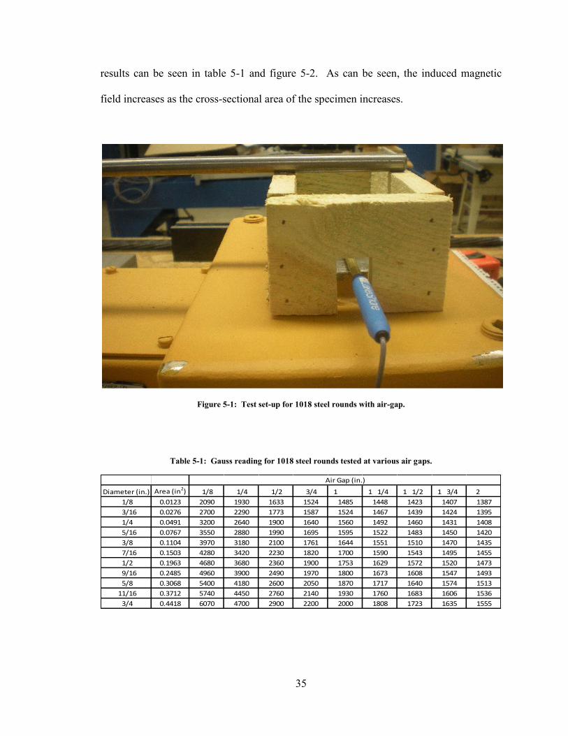
nine different air-gaps. The test set-up for this experiment can be seen in figure 5-1. The

35

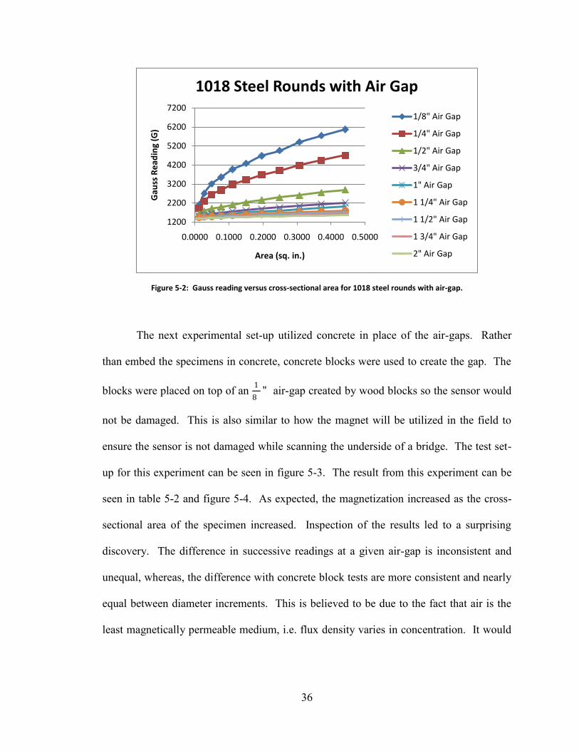
results can be seen in table 5-1 and figure 5-2. As can be seen, the induced magnetic

field increases as the cross-sectional area of the specimen increases.

Figure 5-1: Test set-up for 1018 steel rounds with air-gap.

Table 5-1: Gauss reading for 1018 steel rounds tested at various air gaps.

Diameter (in.) Area (in2) 1/8 1/4 1/2 3/4 1 1 1/4 1 1/2 1 3/4 2

1/8 0.0123 2090 1930 1633 1524 1485 1448 1423 1407 1387

3/16 0.0276 2700 2290 1773 1587 1524 1467 1439 1424 1395

1/4 0.0491 3200 2640 1900 1640 1560 1492 1460 1431 1408

5/16 0.0767 3550 2880 1990 1695 1595 1522 1483 1450 1420

3/8 0.1104 3970 3180 2100 1761 1644 1551 1510 1470 1435

7/16 0.1503 4280 3420 2230 1820 1700 1590 1543 1495 1455

1/2 0.1963 4680 3680 2360 1900 1753 1629 1572 1520 1473

9/16 0.2485 4960 3900 2490 1970 1800 1673 1608 1547 1493

5/8 0.3068 5400 4180 2600 2050 1870 1717 1640 1574 1513

11/16 0.3712 5740 4450 2760 2140 1930 1760 1683 1606 1536

3/4 0.4418 6070 4700 2900 2200 2000 1808 1723 1635 1555

Air Gap (in.)

36

Figure 5-2: Gauss reading versus cross-sectional area for 1018 steel rounds with air-gap.

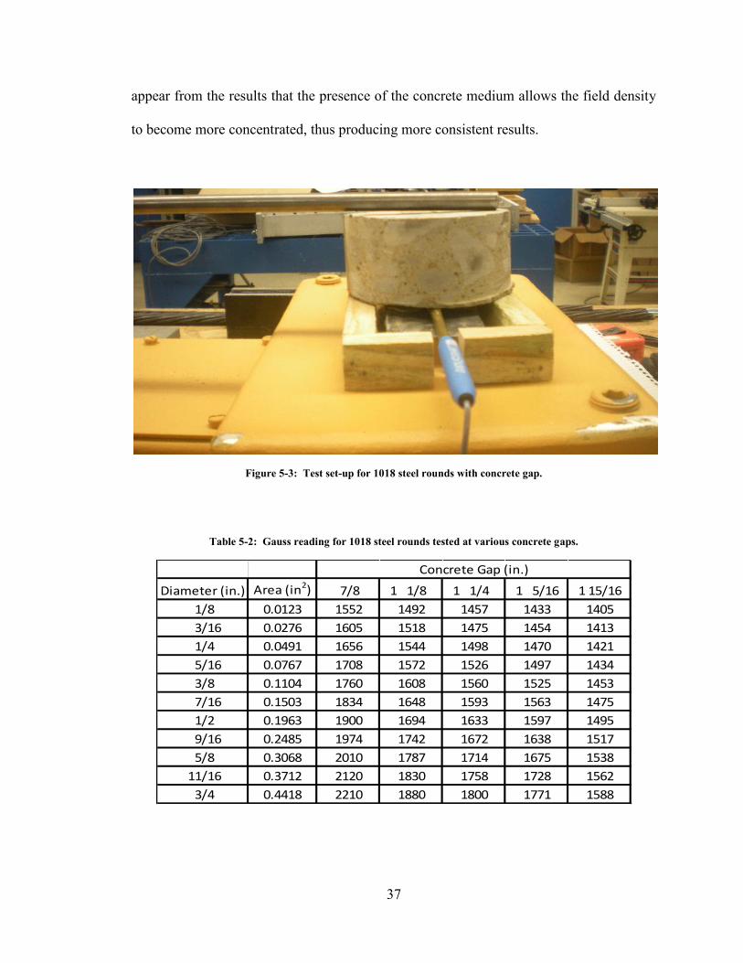
The next experimental set-up utilized concrete in place of the air-gaps. Rather

than embed the specimens in concrete, concrete blocks were used to create the gap. The

blocks were placed on top of an 1

8 " air-gap created by wood blocks so the sensor would

not be damaged. This is also similar to how the magnet will be utilized in the field to

ensure the sensor is not damaged while scanning the underside of a bridge. The test set-

up for this experiment can be seen in figure 5-3. The result from this experiment can be

seen in table 5-2 and figure 5-4. As expected, the magnetization increased as the cross-

sectional area of the specimen increased. Inspection of the results led to a surprising

discovery. The difference in successive readings at a given air-gap is inconsistent and

unequal, whereas, the difference with concrete block tests are more consistent and nearly

equal between diameter increments. This is believed to be due to the fact that air is the

least magnetically permeable medium, i.e. flux density varies in concentration. It would

1200

2200

3200

4200

5200

6200

7200

0.0000 0.1000 0.2000 0.3000 0.4000 0.5000

Gau

ss R

ead

ing

(G)

Area (sq. in.)

1018 Steel Rounds with Air Gap

1/8" Air Gap

1/4" Air Gap

1/2" Air Gap

3/4" Air Gap

1" Air Gap

1 1/4" Air Gap

1 1/2" Air Gap

1 3/4" Air Gap

2" Air Gap

37

appear from the results that the presence of the concrete medium allows the field density

to become more concentrated, thus producing more consistent results.

Figure 5-3: Test set-up for 1018 steel rounds with concrete gap.

Table 5-2: Gauss reading for 1018 steel rounds tested at various concrete gaps.

Diameter (in.) Area (in2) 7/8 1 1/8 1 1/4 1 5/16 1 15/16

1/8 0.0123 1552 1492 1457 1433 1405

3/16 0.0276 1605 1518 1475 1454 1413

1/4 0.0491 1656 1544 1498 1470 1421

5/16 0.0767 1708 1572 1526 1497 1434

3/8 0.1104 1760 1608 1560 1525 1453

7/16 0.1503 1834 1648 1593 1563 1475

1/2 0.1963 1900 1694 1633 1597 1495

9/16 0.2485 1974 1742 1672 1638 1517

5/8 0.3068 2010 1787 1714 1675 1538

11/16 0.3712 2120 1830 1758 1728 1562

3/4 0.4418 2210 1880 1800 1771 1588

Concrete Gap (in.)

38

1400

1600

1800

2000

2200

2400

0.0000 0.1000 0.2000 0.3000 0.4000 0.5000

Gau

ss R

ead

ing

(G)

Area (sq. in.)

1018 Steel Rounds with Concrete Gap

7/8" Gap

1 1/8" Gap

1 1/4" Gap

1 5/16" Gap

1 15/16" Gap

Figure 5-4: Gauss reading vs. cross-sectional area for 1018 steel rounds with concrete gap.

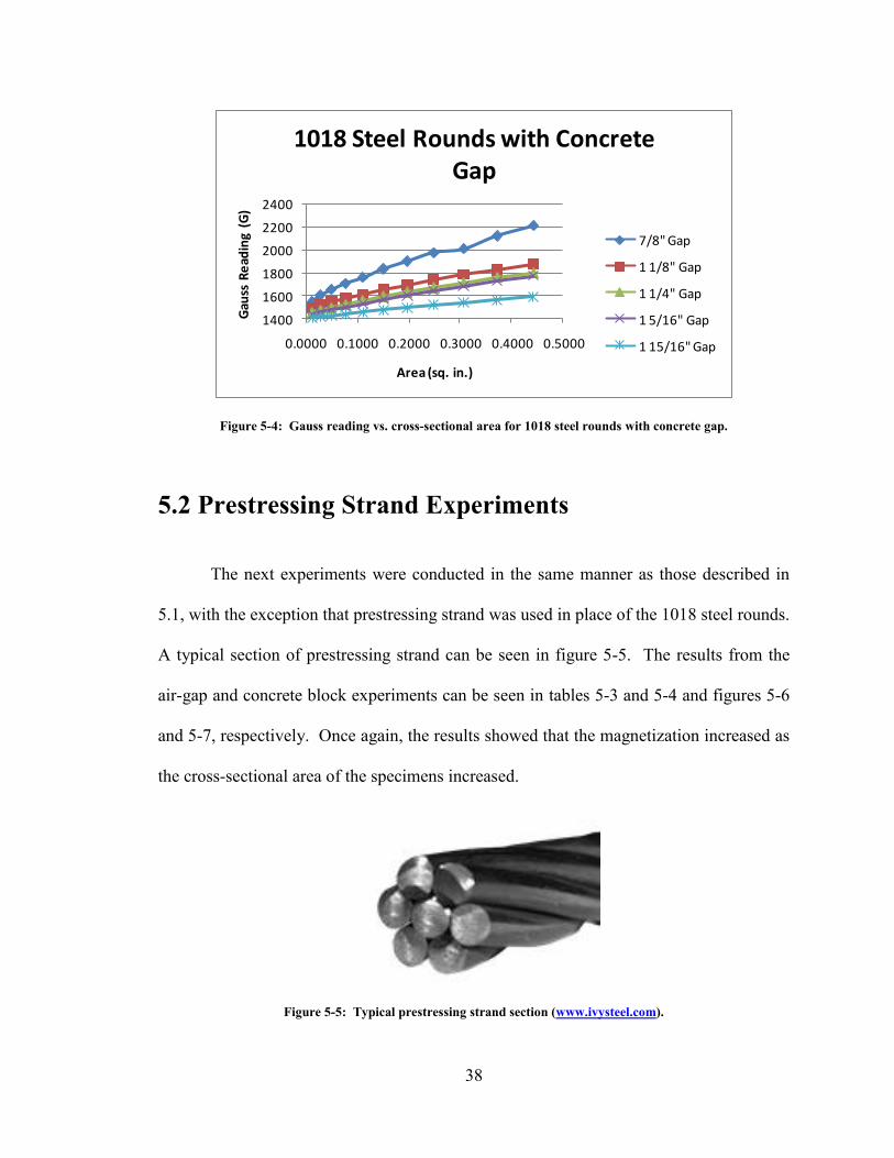
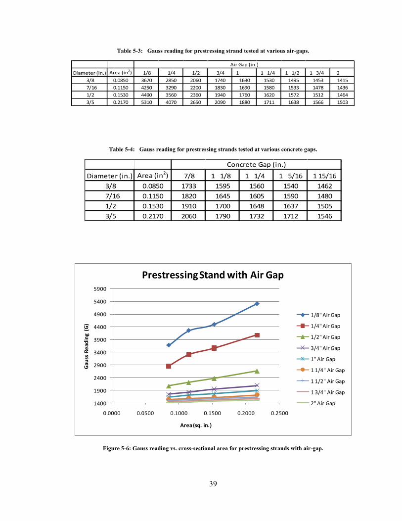
5.2 Prestressing Strand Experiments

The next experiments were conducted in the same manner as those described in

5.1, with the exception that prestressing strand was used in place of the 1018 steel rounds.

A typical section of prestressing strand can be seen in figure 5-5. The results from the

air-gap and concrete block experiments can be seen in tables 5-3 and 5-4 and figures 5-6

and 5-7, respectively. Once again, the results showed that the magnetization increased as

the cross-sectional area of the specimens increased.

Figure 5-5: Typical prestressing strand section (www.ivysteel.com).

http://www.ivysteel.com/

39

Table 5-3: Gauss reading for prestressing strand tested at various air-gaps.

Diameter (in.) Area (in2) 1/8 1/4 1/2 3/4 1 1 1/4 1 1/2 1 3/4 2

3/8 0.0850 3670 2850 2060 1740 1630 1530 1495 1453 1415

7/16 0.1150 4250 3290 2200 1830 1690 1580 1533 1478 1436

1/2 0.1530 4490 3560 2360 1940 1760 1620 1572 1512 1464

3/5 0.2170 5310 4070 2650 2090 1880 1711 1638 1566 1503

Air Gap (in.)

Table 5-4: Gauss reading for prestressing strands tested at various concrete gaps.

Diameter (in.) Area (in2) 7/8 1 1/8 1 1/4 1 5/16 1 15/16

3/8 0.0850 1733 1595 1560 1540 1462

7/16 0.1150 1820 1645 1605 1590 1480

1/2 0.1530 1910 1700 1648 1637 1505

3/5 0.2170 2060 1790 1732 1712 1546

Concrete Gap (in.)

1400

1900

2400

2900

3400

3900

4400

4900

5400

5900

0.0000 0.0500 0.1000 0.1500 0.2000 0.2500

Gau

ss R

ead

ing

(G)

Area (sq. in.)

Prestressing Stand with Air Gap

1/8" Air Gap

1/4" Air Gap

1/2" Air Gap

3/4" Air Gap

1" Air Gap

1 1/4" Air Gap

1 1/2" Air Gap

1 3/4" Air Gap

2" Air Gap

Figure 5-6: Gauss reading vs. cross-sectional area for prestressing strands with air-gap.

40

1450

1650

1850

2050

2250

0.0000 0.0500 0.1000 0.1500 0.2000 0.2500

Gau

ss R

ead

ing

(G)

Area (sq. in.)

Prestressing Strand with Concrete Gap

7/8" Gap

1 1/8" Gap

1 1/4" Gap

1 5/16" Gap

1 15/16" Gap

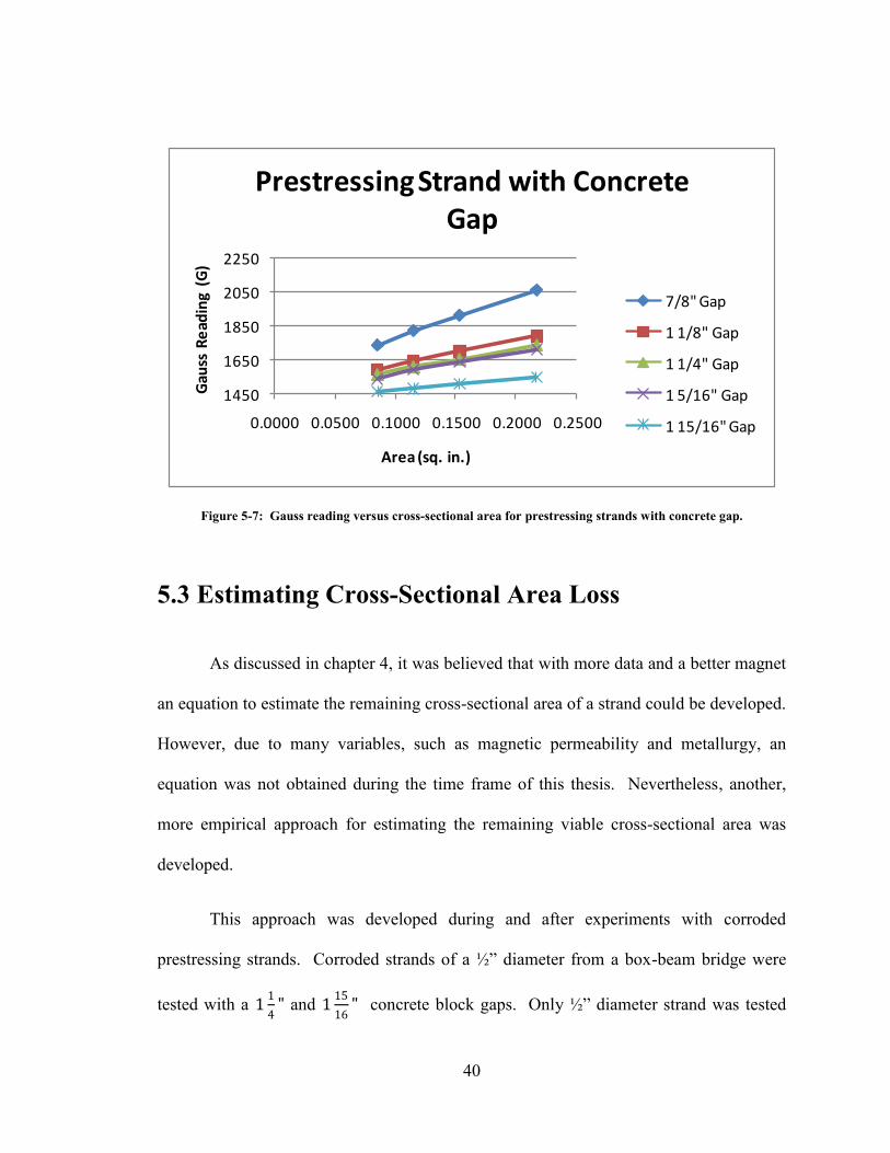
Figure 5-7: Gauss reading versus cross-sectional area for prestressing strands with concrete gap.

5.3 Estimating Cross-Sectional Area Loss

As discussed in chapter 4, it was believed that with more data and a better magnet

an equation to estimate the remaining cross-sectional area of a strand could be developed.

However, due to many variables, such as magnetic permeability and metallurgy, an

equation was not obtained during the time frame of this thesis. Nevertheless, another,

more empirical approach for estimating the remaining viable cross-sectional area was

developed.

This approach was developed during and after experiments with corroded

prestressing strands. Corroded strands of a ½” diameter from a box-beam bridge were

tested with a 11

4" and 1

15

16" concrete block gaps. Only ½” diameter strand was tested

41

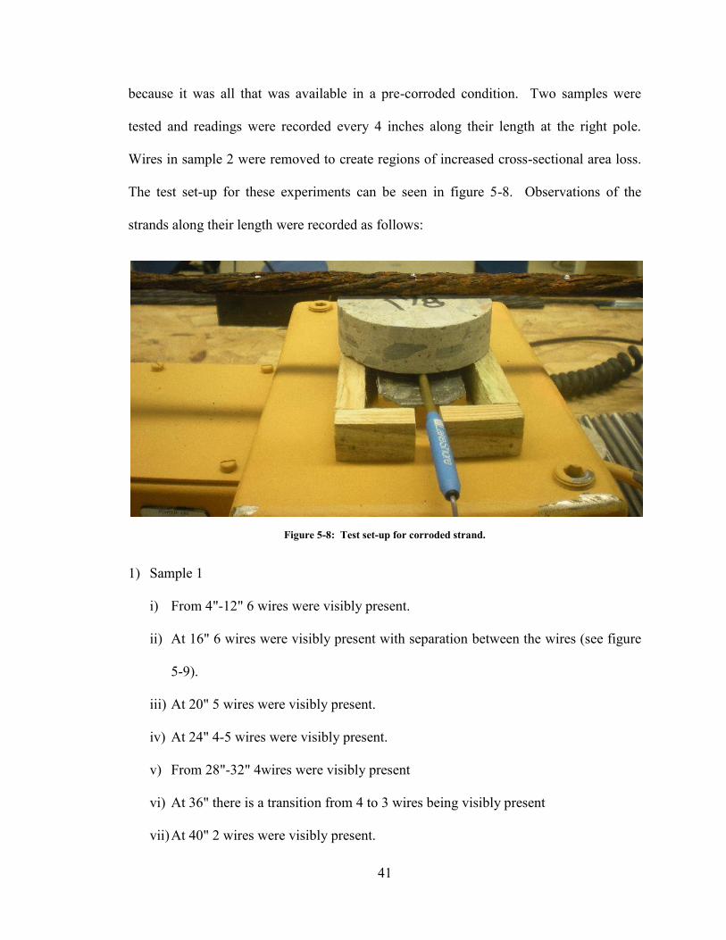
because it was all that was available in a pre-corroded condition. Two samples were

tested and readings were recorded every 4 inches along their length at the right pole.

Wires in sample 2 were removed to create regions of increased cross-sectional area loss.

The test set-up for these experiments can be seen in figure 5-8. Observations of the

strands along their length were recorded as follows:

Figure 5-8: Test set-up for corroded strand.

1) Sample 1

i) From 4"-12" 6 wires were visibly present.

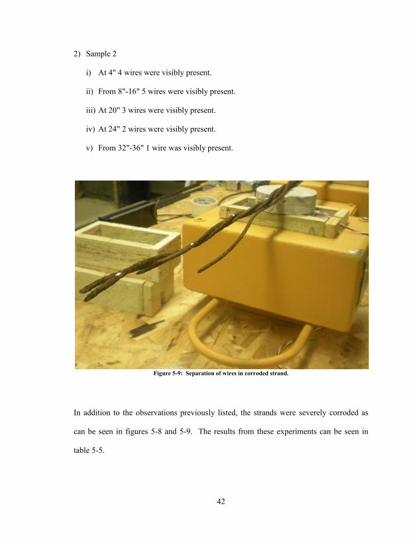
ii) At 16" 6 wires were visibly present with separation between the wires (see figure

5-9).

iii) At 20" 5 wires were visibly present.

iv) At 24" 4-5 wires were visibly present.

v) From 28"-32" 4wires were visibly present

vi) At 36" there is a transition from 4 to 3 wires being visibly present

vii) At 40" 2 wires were visibly present.

42

2) Sample 2

i) At 4" 4 wires were visibly present.

ii) From 8"-16" 5 wires were visibly present.

iii) At 20" 3 wires were visibly present.

iv) At 24" 2 wires were visibly present.

v) From 32"-36" 1 wire was visibly present.

Figure 5-9: Separation of wires in corroded strand.

In addition to the observations previously listed, the strands were severely corroded as

can be seen in figures 5-8 and 5-9. The results from these experiments can be seen in

table 5-5.

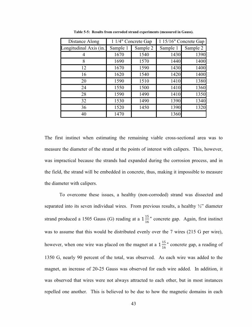
43

Table 5-5: Results from corroded strand experiments (measured in Gauss).

Sample 1 Sample 2 Sample 1 Sample 21670 1540 1430 13901690 1570 1440 14001670 1590 1430 14001620 1540 1420 14001590 1510 1410 13801550 1500 1410 13601590 1490 1410 13501530 1490 1390 13401520 1450 1390 13201470 1360

Distance Along

40

1 1/4" Concrete Gap 1 15/16" Concrete Gap

2024283236

Longitudinal Axis (in.)48

1216

The first instinct when estimating the remaining viable cross-sectional area was to

measure the diameter of the strand at the points of interest with calipers. This, however,

was impractical because the strands had expanded during the corrosion process, and in

the field, the strand will be embedded in concrete, thus, making it impossible to measure

the diameter with calipers.

To overcome these issues, a healthy (non-corroded) strand was dissected and

separated into its seven individual wires. From previous results, a healthy ½” diameter

strand produced a 1505 Gauss (G) reading at a 115

16" concrete gap. Again, first instinct

was to assume that this would be distributed evenly over the 7 wires (215 G per wire),

however, when one wire was placed on the magnet at a 115

16" concrete gap, a reading of

1350 G, nearly 90 percent of the total, was observed. As each wire was added to the

magnet, an increase of 20-25 Gauss was observed for each wire added. In addition, it

was observed that wires were not always attracted to each other, but in most instances

repelled one another. This is believed to be due to how the magnetic domains in each

44

wire align themselves in the field. The orientation of one wire to another produces a give

and take affect that results in a net magnetization of 1505 G when they are all together.

With the data and observations from the experiments, an approach to estimate the

remaining viable cross-sectional area was proposed.

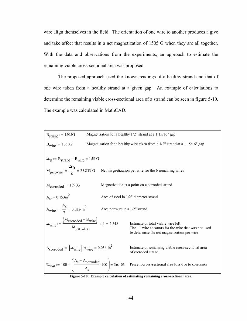
The proposed approach used the known readings of a healthy strand and that of

one wire taken from a healthy strand at a given gap. An example of calculations to

determine the remaining viable cross-sectional area of a strand can be seen in figure 5-10.

The example was calculated in MathCAD.

Figure 5-10: Example calculation of estimating remaining cross-sectional area.

Bstrand 1505G:= Magnetization for a healthy 1/2" strand at a 1 15/16" gap

Bwire 1350G:= Magnetization for a healthy wire taken from a 1/2" strand at a 1 15/16" gap

B Bstrand Bwire- 155 G=:=

Mper.wireB

625.833 G=:= Net magnetization per wire for the 6 remaining wires

Mcorroded 1390G:= Magnetization at a point on a corroded strand

As 0.153in2:= Area of steel in 1/2" diameter strand

AwireAs7

0.022 in2=:= Area per wire in a 1/2" strand

wireMcorroded Bwire-( )

Mper.wire1+ 2.548=:= Estimate of total viable wire left

The +1 wire accounts for the wire that was not usedto determine the net magnetization per wire

Acorroded wire Awire 0.056 in2=:= Estimate of remaining viable cross-sectional area

of corroded strand.

%lost 100As Acorroded-

As100

- 36.406=:= Percent cross-sectional area loss due to corrosion

45

In this example, the observed reading of 1390 G was taken from sample 1 at 36” along

its length where it was observed that 3 to 4 wires were present. If 3 to 4 healthy wires

were present there would be a cross-sectional area of 0.066 in2 to 0.087428 in2. The

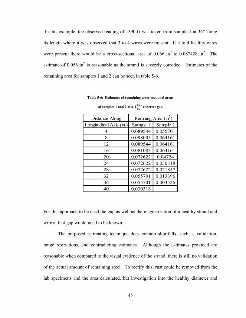
estimate of 0.056 in2 is reasonable as the strand is severely corroded. Estimates of the

remaining area for samples 1 and 2 can be seen in table 5-6.

Table 5-6: Estimates of remaining cross-sectional areas

of samples 1 and 2 at a 𝟏 𝟏𝟓

𝟏𝟔" concrete gap.

Sample 1 Sample 20.089544 0.0557010.098005 0.0641610.089544 0.0641610.081083 0.0641610.072622 0.047240.072622 0.0303180.072622 0.0218570.055701 0.0133960.055701 0.0035260.030318

Distance Along

16202428323640

Remaing Area (in2)Longitudinal Axis (in.)

48

12

For this approach to be used the gap as well as the magnetization of a healthy strand and

wire at that gap would need to be known.

The purposed estimating technique does contain shortfalls, such as validation,

range restrictions, and contradicting estimates. Although the estimates provided are

reasonable when compared to the visual evidence of the strand, there is still no validation

of the actual amount of remaining steel. To rectify this, rust could be removed from the

lab specimens and the area calculated, but investigation into the healthy diameter and

46

area of a ½” nominal strand has hindered this attempt. The area of steel listed with a ½”

strand is 0.153in2 which when distributed over seven wires yields 0.021857in2 per wire.

This in turn yields a calculated diameter of 0.1668in., which does not match the measured

diameter of 0.130in. The area of 0.153in2 may be nominalized and be the reason for this

discrepancy. Neither the ASTM nor other publications have an explanation of how the

area is calculated or give an approximate diameter size for the wires that are to be used in

the strand. Investigation into this issue will need to be continued so this or any other

estimation approach can be properly calibrated.

Another shortcoming of this approach may be attributed to inadequate field

strength. As previously mentioned, the magnetization of one wire is 1350G, which is

within the range of the estimating approach, but once the magnetization drops below

approximately 1320G the estimate increases from the expected. One explanation of this

discrepancy is due to the field strength of the magnet being used.

The field strength of the magnet alone on the right pole is 1460G. At 115

16"

concrete gap a ½” diameter strand has a magnetization of 1505G. From other specimens

tested at smaller gaps, it is known that the magnetization of a ½” diameter specimen is

capable of being higher. As with the first magnet at this distance, there is less

magnetization. In short, the magnetic capacity of the strand is not being filled. However,

at this same distance (1 15

16") the wire’s capacity may be filled or at least have a higher a

higher degree of saturation to area than the strand. This cause’s a few problems when

trying to estimate the area. The estimation is more or less based on a linear approach, but

the data show that the magnetization although nearly linear, is curved. Nevertheless, it

47

appears that this causes the estimates to err on the side of caution, i.e. there is more area

remaining than estimated.

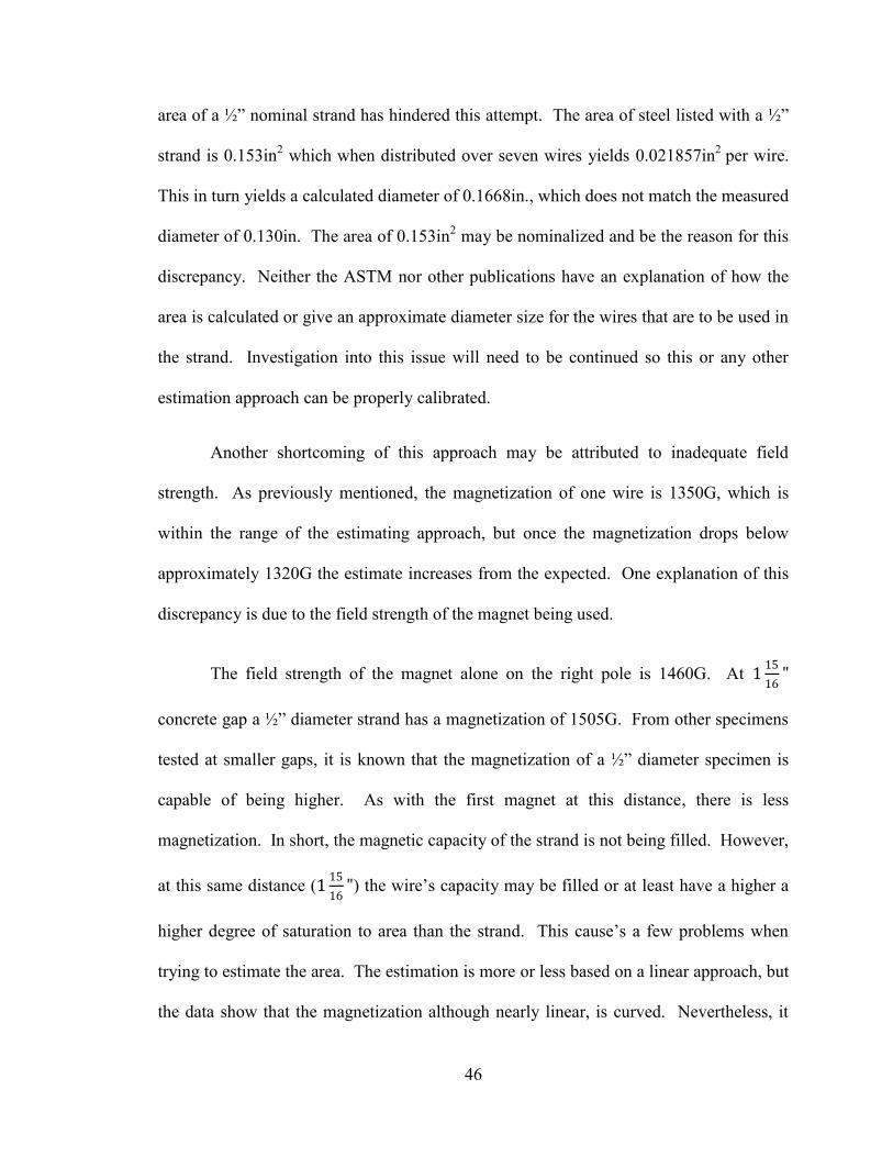
The other problem is that there could be two estimates for a magnetization of

1460G; 0in2 or 0.115in2 for this region. Since the magnetization curve of a strand or any

other ferromagnetic material is non-linear (see figure 5-11), there will be errors when

estimating the area. Nonetheless, these errors could be minimized by optimizing the

electromagnet design for size of specimens and gap being tested for. In other words, if

the field strength were increased to ensure the specimens being magnetized would be at

or near complete saturation, the error in estimating would be reduced as the data would

become more linearized. Until such an electromagnet becomes available, the estimating

approach proposed here gives reasonable, conservative estimates and, with more testing

and scrutinization, could become an effective estimating tool.

Figure 5-11: Magnetization curve for iron (http://info.ee.surrey.ac.uk/Workshop/advice/coils/mu/BH_iron.png)

48

Chapter 6 Conclusion 6.1 Results

The results obtained thus far are promising that this will develop into a new

magnetic NDE technique. A consistent reliable relationship between cross-sectional area

and magnetization was found for a variety of steel specimens, including corroded

prestressing strand at varying distances from the magnet face. It was observed that as the

cross-sectional area of the specimens increased so did the magnetization. An approach

for estimating the remaining area of corroded strands was developed. The estimate

results seemed reasonable when compared with visual inspection of the strand. This

research has demonstrated that the proposed electromagnetic system for detection of

corrosion in deteriorated prestressing strand has significant potential. The primary

objective, proof of concept, was achieved.

6.2 Future Research

Thus far, the research and results have demonstrated that the technique proposed

in this thesis has potential. To further validate this technique more laboratory

49

experiments, field tests, and theoretical work must be completed. Laboratory testing

should consist of embedding strands in concrete at various distances. These experiments

should be used to validate and calibrate, or invalidate the estimating method proposed in

Chapter 5. Also, water content is believed to affect the magnetization of the strands, so

testing should be done at various time intervals as the concrete hardens and the water

content decreases. In addition, the influence of neighboring prestressing strands and/or

mild reinforcement needs to be investigated. These experiments should be similar in

geometric configuration as what can be expected in a bridge beam.

Field tests would involve the scanning of a beam on an existing bridge. A

bridge scheduled for demolition by ODOT has been identified as a potential candidate for

field testing. However, before field testing could be done, a carriage system for the

magnet needs to be developed. Currently, this system is being developed at The

University of Toledo.

Data acquisition and analysis would also need to become quicker and

computerized. Currently, a data acquisition system has been used to re-complete the

preliminary experiments with the 1018 steel rounds. However, it was discovered that the

Hall sensors being used did not have the capacity to produce accurate results at certain

gaps and specimen diameters. New sensors for this system are being ordered, as well as

transitioning the system from a desktop computer to a laptop.

The complexity of this technique also requires that an expert in metallurgy be

consulted. It is known that the magnetic properties are changed with the introduction of

defects, such as dislocations, grain boundaries, and boundaries between phases in the

atomic structure. Also, the stress state of the strand will change its magnetic properties.

50

The unknown is how much these defects and the stress state will affect the overall

estimate of remaining cross-sectional area and how they can be accounted for. With new

experimental data and metallurgical data, the estimating approach proposed can be

calibrated or a new approach can be developed to estimate the remaining cross-sectional

area. In addition, the metallurgical data may be helpful in adjusting known theorectical

equations for net magnetization to produce more accurate estimates. As with any

research endeavor, there is a chance of failure, but nothing thus far has shown that this is

impossible.

51

References

Ali, M, Maddock, A. “Evaluation of Corrosion of Prestressing in Concrete Using Non- destructive Techniques.” GHD Pty Ltd., Sydney. 2003. Askeland, D. The Science and Engineering of Materials. Massachusetts. PWS-KENT Publishing Company. 1984. FHWA. “Corrosion Costs And Preventive Strategies in the United States.” http://www.corrosioncost.com/pdf/techbreif.pdf. March 2002. Hillemeier B, Scheel H. “Magnetic Detection of Prestressing Steel Fractures in

Prestressed Concrete.” Materials and Corrosion. 1998. Indacochea, J, Rumiche, F, Wang, M. “Assessment of the Effect of Microstructure on

the Magnetic Behavior of Structural Carbon Steels Using an Electromagnetic Sensor.” Journal of Materials Engineering and Performance. September 2007.

Nims, D. “Nondestructive Inspection of Deteriorated Prestressing Tendons in Concrete

Bridges.” The University of Toledo. March 2008. Devabhaktuni, V, Nims, D. “Magnetic Sensor for Nondestructive Evaluation of

Deteriorated Prestressing Strand.” The University of Toledo. December 2008.

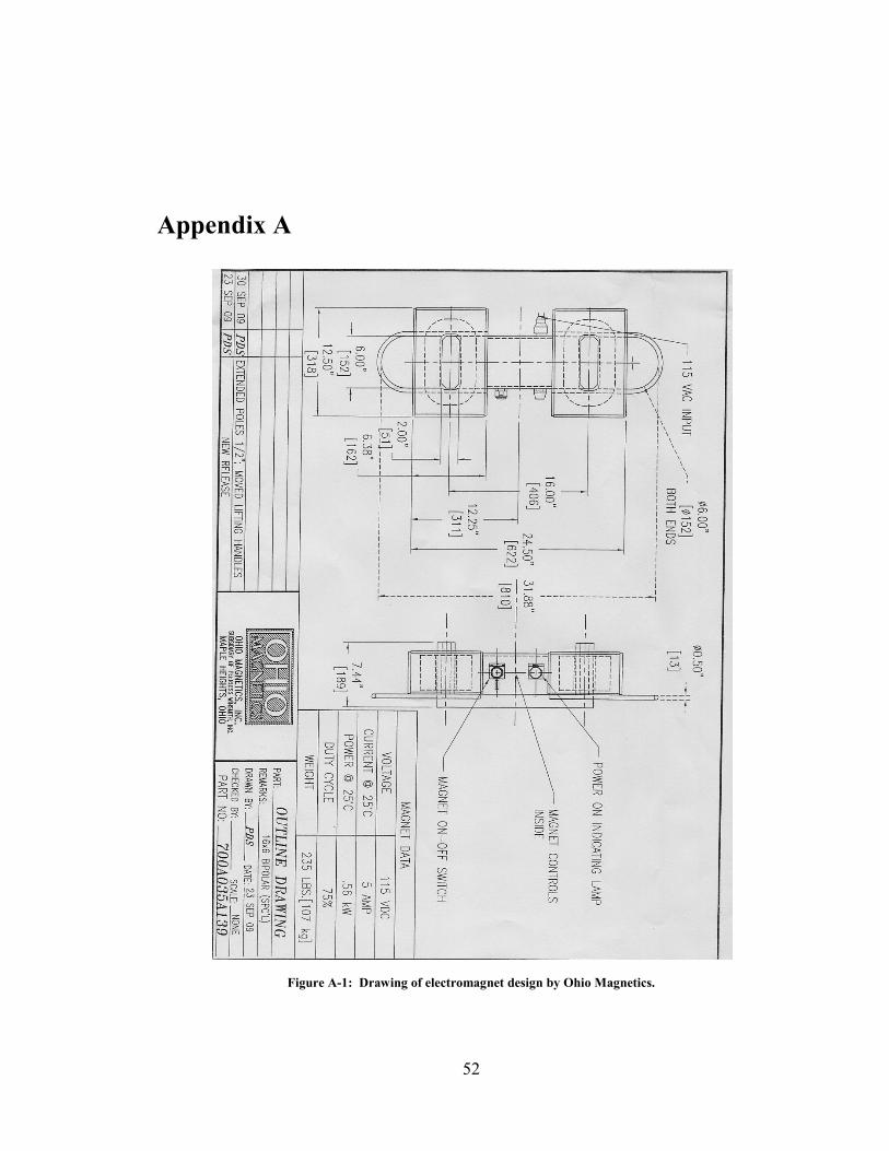
http://www.corrosioncost.com/pdf/techbreif.pdf

52

Appendix A

Figure A-1: Drawing of electromagnet design by Ohio Magnetics.

A New Magnetic Sensor Concept for Nondestructive Evaluation of Deteriorated Prestressing Strand

Documents

Transcript of A New Magnetic Sensor Concept for Nondestructive Evaluation of Deteriorated Prestressing Strand