~ ) Pergamon Microelectron. Reliah., Vol. 36, No. 1, pp. 71-81, 1996

Copyright © 1995 Elsevier Science Lid Printed in Great Britain. All rights reserved

0026-2714/96 $9.50 + .00 0026-2714(95) 00056-9

A NEW DEVELOPED TRANSIENT-BEHAVIOUR SOLUTION TECHNIQUE FOR RELIABILITY EVALUATION OF ELECTRICAL SYSTEMS

ISA S. QAMBER and ADEL A. KAMAL

Electrical Engineering Dept, College of Engineering, University of Bahrain, P.O. Box 3:3831, Isa Town, Bahrain

(Received for publication 17 February 1995)

ABSTRACT

Transient probability prblems were studied in four three-state power system and one seven state telecommunication system. The study was carried out using the Adams Method and another method which is developed for this study. The new method is named as Stabilization Method (SM). The new method is compared with Adams method from stability and accuracy view points. It was found that the SM method required less programing effort compared to the Adams method. The accuracy of stabilization method (SM) compares well with Adams when sufficiently small time interval is chosen. The relationship between the CPU time and the number of states was found to be non-linear for the SM method

INTRODUCTION

It is well known that reliability studies can be applied to many fields and equipment. Biomedical instruments, telecommumcation models, electrical generators and other systems can be studied. Transient solutions are important when it is required to study the behaviour of a system immediately after starting-up, after repair or if the behaviour is required over a fixed period during which the system is to perform a given mission. Several methods are available to solve the first order differential equations, which are; Unmodified Euler method, Modified Euler method, Fourth- order Runge-Kutta method, Milne's method and Adam's method.

The modified Euler's method advantage over the un-modified one is its error term reduction whilest the Fourth-order Runge-Kutta method is more accurate than the previous two methods. The Milne's method is a multistep predictor-corrector method. The disadvantage of this method is that it is not self-starting and also it produces numerical evaluation instabilities. The Adam's method is also not a self-starting method but, because of its superior accuracy and stability, it was chosen as a comparison method with the developed method to obtain both the steady- state and transient solutions of different state models. The solutions of the Adams Method and the developed method, which is subsequently called the Stabilization Method, are investigated to establish the deference between the two methods with regards to their stability and the accuracy of their solutions.

71

72 I.S. Qamber and A. A. Kamal

Many engineering problems produce not only one but several differential equations. These equations need to be solved simultaneously[I]. Most conveniently, this set of first order differential equations can be written in the following form[2] :

~t : ~d ' t 'P ' 'P~ ........ P°5

ap~

- 2 . ~ . t , p , , p : . . . . . . . . p . 5 at

In many applications such as Markov modelling these equations reduce to a linear form •

a p , kt'~

~t

= -a , ,Pd. t '~+ a,~P~ktS+ ...... +a, .P.kt '~

~P~kt5

( l )

ap~kt'~ dt

Equations (1) can be re-written in the simple matrix form as :

Where A is an n by components Pi.

Equation (2) could be used as the starting point for the development of this work.

( 2 )

n matrix with all elements independent of time and

STABILIZATION METHOD (SM)

In many practical problems [3], a natural unit of time often suggests itself, where it could be the year. Transformation from the continuous time to the discrete time domain can be accomplished as follows [6]:

where A is the transition rate matrix, which can be approximated to

where h is a sufficiently small interval of time. This gives :

Reliability evaluation of electrical systems

_v~,~ + ~ - 2 c , ~ ) = ~ . t ~ . ~ i.e ~ ~ + ~a) = ~ , ~ + ~a.k._~,~)

= c,~ +,a. t~'~v_c,~) = "~_v~.~

where T is a transition matrix defmed now by :

T = I + h A

and I is the unit matrix.

(5)

( 6 )

73

The algorithm for the present method can be written as follows :

PI=P, IZP, (7)

All state probabilities at each step of time sum up to unity. To stabilize the results the following equations were derived and then added:

E - m tx- 5 (8)

h3 = h l / n

whe re : h 1 is the 1st step-size used to obtain the estimate value V1

h 2 is the 2nd step-size used to obtain the estimate value V2

h 3 is the 3rd step-size used to obtain the true value to be estimated

m is an integer number used to obtain h 2, h2=hl/m p the order of accuracy which is 2 for the developed

method n is a number calculated using equation (8) to obtain h 3

Because the algorithms performed with any computer involve numbers with a finite number of digits, a rounding error is always associated with the arithmetical calculations. For this reason, the step-size h and the accuracy E cannot be chosen arbitrarly small. They must be chosen such that the corresponding changes in the values of the components of the state vector Pi are significantly greater than the rotmding error[6].

The SM method was programmed in FORTRAN 77 using the University of Bahrain computing facilities. Also, the same facilities were used for the Adam's method.

74 I.S. Qamber and A. A. Kamal

R E S U L T S and D I S C U S S I O N S

The main objective of this section is to compare the solution of certain models using the Adams and stabilization methods. Also some applications of these methods are given.

The results obtained using both methods will be discussed. The criteria used to compare them is the accuracy, the CPU time and the numerical stability of the solution.

(a) Three-state Models :

and Four three-state models that were studied by BIGGERSTAFF

JACKSON[5] for a system comprising of a number of generators will be considered. The common transition rate matrix for each model can be written in the following form :

6 P ~ 3 _ ( 9 )

The numerical values models of the transition rates differ for each of the four models as given in Table 1. The data for these models are based on data [4] relevant to plant operated by Tennessee Valley Authority (TVA). The system is considered to be in one of the following states (as seen in Fig.l) :

i S1 ii - $2

iii- $3

System operates at full capacity System operates at less than full capacity due to generator outages because of forced outages no power at all is generated.

For each model, both methods were used to calculate the state probability variations against time and compare the results with the previous study performed by Biggerstaff and Jackson [5] for time t= 6 hours and t=24 hours, which are reproduced in Table (2). The results of the two methods are summarized in Tables (3 and 4) where, for convenience, the % error in the values obtained by those methods and the

Table 1 : TVA Svstem Confi2uration

Model T . R (1/hr)

a b c d e f

1 0.0003 0.0010 0.0225 0.0350 0.0008 0.0004 2 0.0006 0.0050 0.0400 0.1000 0.0004 0.0004 3 0.0005 0.0002 0.0240 0.0430 0.0001 0.0001 4 0.0010 0.0006 0.0200 0.1000 0.0002 0.0020

(T.R: Transition Rate)

Reliability evaluation of electrical systems

Fig. (1) Three-State Models

75

Table 2 : TVA Results

Model t = 6 hours t = 24 hours

Pup Pdown Pderated Pup Pdown Pderated

1 0.99293 0,00168 0.00539 0.97849 0.00552 0.01599 2 0.97462 0.00318 0.02220 0.94756 0.00906 0.04338 3 0.99616 0,00279 0.00106 0.98798 0.00905 0.00298 4 0.99168 0,00564 0.00268 0.97582 0.01888 0.00530

Table 3 : SM method (Results Fot Models 1, 2, 3 and 4)

Model

h

(hour)

t

(hour)

6

Pup

(% error)

0.01111

Pdown

(% e~or) -1.19043

Pderated

(% error)

-1.66976 24 0,02351 -0.72464 -1.18824

2 6 0.02216 -2.38095 -3.33952 24 6

-1.63043 -1.88679

0.04803 0.09747

-2.37649 -4.00901

24 0.06543 -1.21413 -1.15261 2 6 0.20623 -3.77358 -8.51351

-2.53863 -1.07527

24 6

0.12981 0.00602

-2.30521 -1.88679

24 0.01316 -0.88398 -1.00671 2 6 0.01104 -2.15054 -3.77358

0.02530 0.00017

24 6

-1.87845 -0,01064

-2.34899 -0.04104

24 0.00023 -0.00847 -0.01132 2 6 0.00034 -0.02128 -0.08582

-0.01695 24 0.00045 -0.02453

76 I. S. Qamber and A. A. Kamal

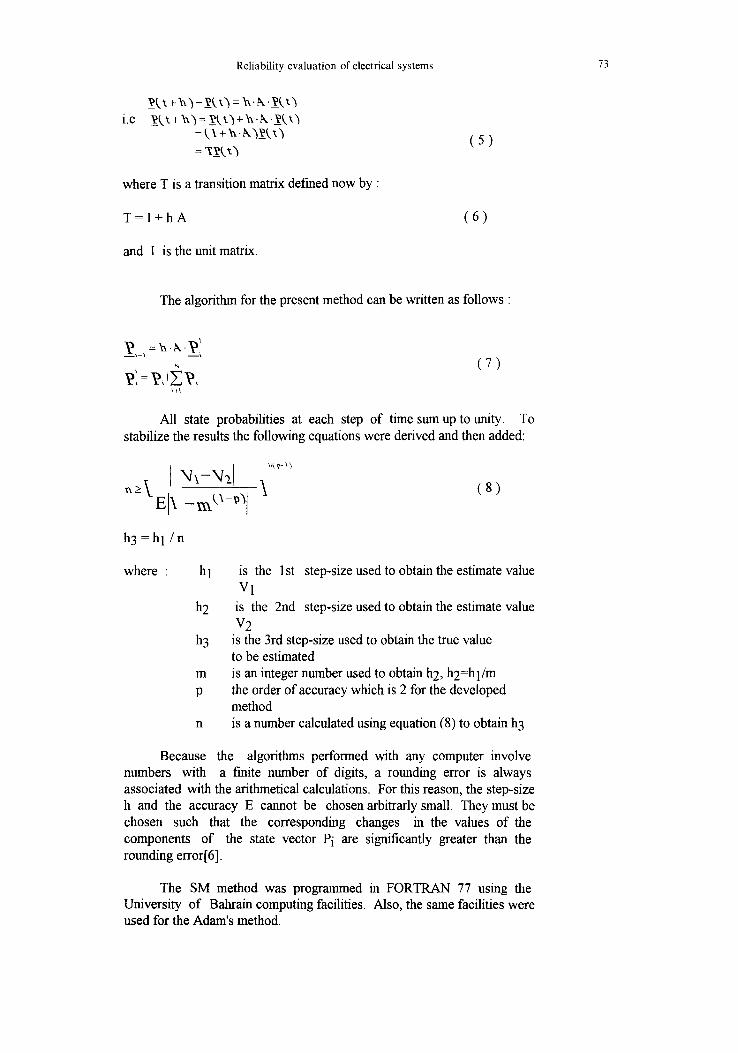
T a b l e 4 : A d a m s M e t h o d Resul t s for ( M o d e l s 1, 2, 3 and 4)

t Pup Pdown Pderated

Model (hour) (% error) (% e~o0 (% e~or)

1 6 -0.00002 0.00000 0.00371 24 -0.00001 0.00181 0.00063

2 6 -0.00002 0.00000 0.00045 24 -0.00001 0.00000 0.00023

3 6 -0.00002 0.00717 0.00943 24 0.00000 0.00110 0.00000

4 6 -0.00001 0.00000 0.00000 24 0.00000 0.00000 0.00000

(Note : Values for h = 1 hour and h = 2 hours are identical)

original TVA results [5] are given by Pup , Pdown and Pderailed, respectively.

It can be seen from Tables 3 and 4 that the Adams method has a very small difference in the percentage error of the transient state probabilities compared to the TVA results, while the difference for the same models using the SM method is increased as the time interval h increases.

(b) Seven-State Model :

The problem used by Barlow and Hunter [7] is reconsidered in the following example. The example is a system consisting of two transmitters A and B and a power supply C providing a high voltage with a modulator and modulation programmer. The two transmitters are run from the same power supply (C).

If one of the two transmitters fails, the other one can perform the system task satisfactorily but with a reduction in response time.

The system is considered as being in one of seven possible states; these are as follows :

S 1: all three units are working properly $2: B and C are working properly, but A fails $3: A and B are working properly, but C fails $4: A and C are working properly, but B fails $5: B is working properly, but A and C fail $6: C is working properly, but A and B fail $7: A is working properly, but B and C fail

The four states $3, $5, $6, and $7 represent the system failures when the system shuts down, requiring repair. In case of the power supply unit failure, the system will fail as a whoal. Similarly, if both transmitters fail, the system serves no purpose and operation is discontinued until

Reliability evaluation of electrical systems 77

repaired. For the above two reasons, the state represented by the failures of all the three units can be ignored ( the state space diagram is given in Fig. 2). The system equations are '

~t &x

a p j , c~ _ %.%%s p,c, tS- ~.%pJ, t'~ at

~ . ~ p , / t s - ~.s%spAts+~.spAtS+~.%pJ, t5 at

6.p~kt'~ _ ~mspAtS_~.%p~k q 6t

,x p~£,Q _ % ~z p~t ' t3 + ~. ~'z p , ~,,q- pJ,~3 &t at

( 1 0 )

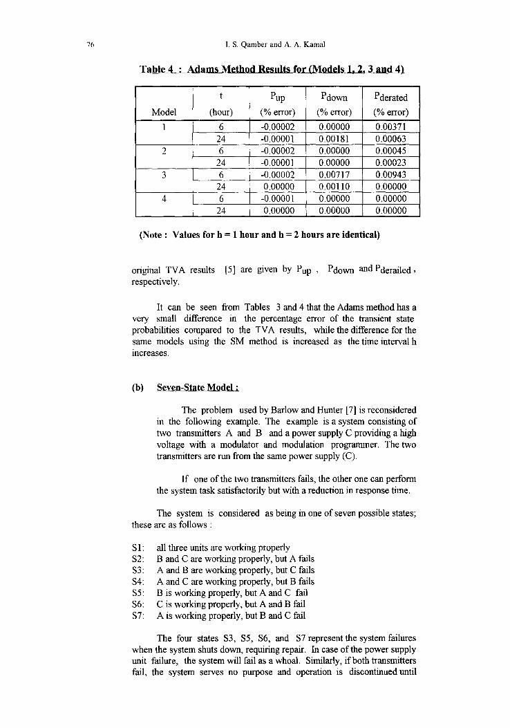
Both methods were applied to the seven state system. Reference calculations in this case are taken from [7] and reproduced in Table 5 (for the first four states only), The results obtained for the SM method are given in Table 6. Using the Adams method, it is found that the percentage error is zero for each step.

It can be seen from the results of the 7-state model that the Adams method produces virtually identical results for the model, surprisingly there are small differences in the results of the four earlier three-state models.

Oz2 ~ 0.005

o . o 1 ~ 0.5

0.2 ~ 0.005

Fig. (2) State Space Diagram for three-unit system

78 I. S. Qamber and A. A. Kamal

Table 5 : State-Probabilities for the First 4 States (7-State Model)

t (hours) Pl(t) P2(t) P3(t) P4(t)

0 1 2 4 8 10

1.000 0.977 0.963 0.948 0.937 0.932

0.000 0.010 0.016 0.022 0.024 0,025

(Note : Results taken from ref. [7])

0.000 0.004 0.008 0.013 0.019 0.022

0.000 0.008 0.012 0.016 0.018 0.019

Table 6 : "SM" Method (Results for 7-State Model)

t (hour)

1 2 4 8 16

P1

(% error)

h=0.5 h=l.0

O.002 0.005 0.003 0.006 0.003 0.005 0.001 0.002 0.000 0.000

P2

(% error)

h=0.5 h--1.0

-0.100 -0.300 -0.125 -0.188 -0.145 -0.045 -0.042 -0.042 0.000 0.000

P3

(% error)

h=0.5 h=l.O

-0.250 -0.250 0.000 -0.125

-0.077 -0.077 0.000 -0.053

-0.045 -0.045

P4

(% error)

h=0.5 h=l.0

-0.125 -0.250 -0.033 -0.167 -0.063 -0.125 -0.056 -0.056 0.000 0.000

CPU Time :

To study the effect of the time interval h on CPU time, the two methods were applied to four state and sixteen state models.

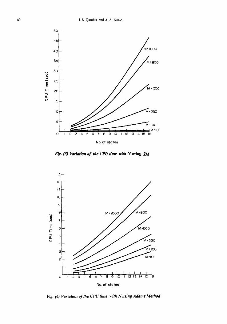
All units are in arbitrary units; a time interval from 0 to 5 units was taken for the two models. The number of steps M is accordingly varried by M=5/h. The results for the two models are given in Figs.3 and 4. From the two figures, it is seen that the relationship between the CPU time and M is approximately linear for the two methods. The two methods were also used to investigate the relationship between the CPU time and the number of states in the model (the results are given in Figs. 5 and 6). It is seen that the curve obtained by the developed method for all evaluations appear to pass through or near the origin. It is clear from Fig.5 and 6 that the CPU time increases nonlinearly as the number of states increase.

CONCLUSION

It can be conclude that the Adams method was stable for all values of h. The minor disadvantage of Adams method that it is relatively complex to program and it requires a subroutine to generate starter values. The stabilization method has a number of advantages. One of its

Reliability evaluation of electrical systems 79

6 . 0 - -

5.5

5.0

4 .5

"" 4 .0

3 5 i p 3 o

2 .5

o 2.0

1.5

1.0

0 .5

0 I I I I I I I I I I

I00 200 500 400 .500 600 700 800 900 I000

No. of evaluation in run (M)

Fig. (3) Variation of the CPU time with M (Case # I)

0 ID tO

ID

E k-

o.. o

65 60

55

50

45

40

:55

:50

25

20

15

I0

5

0 - I ~ " ~ 1 " ~ ' ~ 1 I I I I I I I I

I00 200 300 400 500 600 700 800 900 I000

No. of evaluation in run (M)

Fig. (4) Variationof the CPU time with M (Case # 2)

NR 36-1-F

80 I.S. Qamber and A. A. Kamal

v

E I--

13_ 0

5o I -

4 5 -

4 0 -

3 5 -

3 0 -

2 5 -

i

2 0 -

151-

I 000

=800

= 500

I0

5

0

M = 2 5 0

~ M =100

~ M = I O I 2 3 4 5 6 7 8 9 I0 I I 12 13 14 15 16

No, of s ta tes

Fig. (5) Variation of the CPU time with N using SM

12~--

8 @)

7 v

.E_ 6

5 13_ 0

4

M = ~000 / / M : 8 0 0

~00

:50

M=IO

I 2 3 4 5 6 7 8 9 I0 I I 12 13 14 15 16

No. of s ta tes

Fig. (6) Variation of the CPU time with N using Adams Method

Reliability evaluation of electrical systems 81

advantages is its simplicity of formulation. Also, it is easy to program and incorporate as a subroutine in other programs. The principal disadvantage is that numerical instability of the solution can occur if a step size h is chosen significantly greater than the reciprocal of the smallest element in the transition rate matrix.

ACKNOWLEDGEMENT

We wouM like to express our appreciation to Dr. A, Z Keller for his contmuous help and to University of Bahrain for providing the facilities to conduct this research.

R E F E R E N C E S

. Morris, W.D, "Differential equations for Engineers and applied Scientists", McGraw-Hill, UK, 1974.

. Campbel, S.L, "An Introduction to differential equations and their Applications", Longman Inc., 1986.

. Keller, A.Z, "Markov chains and Monte Carlo Simulation Methods", Lecture Note NO. 4, School of Industrial Technology, University of Bradford.

. Billinton, R & Jain, A.V, "Unit derating in spinning reserve studies", IEEE Trans. on PAS, Vol.90, No.4, pp. 1677-1687, 1971.

. Biggerstaff, B.E & Jackson, T.M, "The Markov process as a Means of determining generating-unit state probabilities for use in spinning reserve applications", IEEE Trans. on PAS, Vol.88, No.4. pp.423- 430, 1969.

. Gerald, C.F & Wheatley, P.O, "Applied Numerical Analysis", Addison Wesley, 1984.

. Barlow & Hunter, "System Efficiency and Reliability", IRE National Convention Proceedings, Vol. 7, No. 6, 1959, pp. 104- 109.