A MULTIMETHOD EXPERIMENTAL INVESTIGATION OF THE EFFECT OF MARKET PRICE KNOWLEDGE ON ACCEPTABLE PRICE RANGE

by

RUSTAN KOSENKO

DISSERTATION submitted to the Faculty of the

Virginia Polytechnic Institute and State University

in partial fulfilment of the requirements for the degree of

APPROVED:

-JK~nt B. ti~h;oe .. (Co-Chairman)

- CaiiiIIIe P. Schuster

DOCTOR OF PHILOSOPHY

in

GENERAL BUSINESS

Rammohan Pisharodi

--M:'Jq~ir~y~-.,,,.,,, (Co-Chairman)

Robert S. Schulman

I

"

A MULTIMETHOD EXPERIMENTAL INVESTIGATION OF THE EFFECTS OF

MARKET PRICE KNOWLEDGE ON ACCEPTABLE PRICE RANGE

by

Rustan Kosenko

(ABSTRACT)

This dissertation reports a multimethod investigation of the

relationship between market price knowledge and the width of the

acceptable price range. Psychophysics and Social judgment theory

are discussed as supporting the existence of acceptable price

thresholds (limits) and acceptable price range. Hypotheses

stemming from Social judgment theory are offered directly

relating market price knowledge with the width of the acceptable

price range.

The relationship between market price knowledge and

acceptable price rangewas investigated using two different

methods, the Stoetzel and the Own-Category method. Unlike the

previous acceptable pr ice 1 imi t studies, this research assessed

the reliability and construct validity of each of those methods.

The research design used was a laboratory experiment with a

series of 2 x 2 factorials based on the Solomon 4 group-six study

design. The dependent variables were: (1) the acceptable lower

price limit, (2) the acceptable upper price limit, and (3) the

acceptable price range. The independent variable was market price

knowledge. The two-way anova design had two factors. The first

factor had two levels: absence and presence of market price

knowledge. The second factor consisted of two levels: pretest and

no pretest treatments.

The research hypothesis was tested using ( 1) two-way

analysis of variance, (2) analysis of covariance using sex and

prior price knowledge as covariates, and (3) paired t-tests.

Test-retest reliability of the two methods were assessed

using Pearson's correlation coefficient. Pearson correlation

coefficients were also used to set validity coefficients. Those

coefficients were used to assess construct validity of the two

measures in terms of convergent and discriminant validity within

the context of Campbell and Fiske's multitrait-multimethod zero-

order correlation matrix.

In general, the experimental results partially confirmed the

hypothesis that the acceptable price range would be narrower for

subjects possessing market price knowledge than for those

subjects possessing little or no market price knowledge. The

results of the Stoetzel method supported the hypothesis, but the

hypothesis was not supported when the same subjects used the Own-

Ca tegory method.

The results did support the hypothesis that the two methods

were valid measures of ac~eptable price thresholds with the Own-

Ca tegory method producing higher reliability scores than the

Stoetzel method.

Results of the dissertation are discussed with respect to

the major findings and significance to price theory and research.

The dissertation concludes w"ith a discussion of the study

limitations and directions for future research.

ACKNOWLEDGEMENTS

No dissertation or any research of substance can be

considered the sole result of the efforts of the individual whose

name appears as the author. Rather, this research is the result

of a group of individuals who so freely shared their knowledge

and expertise with me.

I am greatly endebted to Professors Kent B. Monroe and M.

Joseph Sirgy who served as co-chairmen of my dissertation

committee during the final stages of this research. Their advice

and encouragement not only greatly adhanced the quality of the

research, but contributed to my professional growth. Moreover,

their thoughtful and quick editorial turnaround time during the

dissertation expedited its completion. I will always be grateful

to them for teaching me the importance of theory and research

methodolbgy within the realm of Philosophy of Science.

Sincere appreciation is also extended to Professors Camille

M. Schuster and Rammohan Pisharodi for their advise and helpful

comments during various stages of the dissertation. Equally

important to the completion of this dissertation was the advice

and support offered by Professor Robert S. Schulman. He taught me

that sound theory and good research design are in themselves

insufficient conditions for quality research. Rather statistical

design must be incorporated within the entire research process to

enhance the inferential conclusions.

Most importantly, very special thanks must go to my former

dissertation chairman, Professor Jeffrey E. Danes, who

iv

unfortunately moved to another university before the dissertation

was completed. Nonetheless, he was my major mentor during the

entire dissertation period, and had I not procrastinated the

dissertation would have been completed under his chairmanship. He

continued to make insightful comments and provided advise even

after leaving Virginia Tech. I will always cherish the friendship

we developed during the past years. I look forward to seeking his

advise and counsel in the future as I pursue other research

endeavors.

I would also like to thank Dean Randolph E. Ross, Professor

Peter M. Banting, and Professor George 0. Wesolowsky from

McMaster University for their continued support. I regret that I

was not able to complete this dissertation while a member of

their faculty.

Professor Kahandas Nandola, my chairman at Ohio University,

provided me with the advise and support I needed to expedite the

completion of the final drafts of the dissertation with minimal

distractions. Also, I appreciate the support provided by

Professors Tim Hartman and Ashok Gupta during the last few months

of tempermental behavior.

Finally, I will forever be indebted to my family for their

support and understanding during the entire period of this

sojourn. Noteably, my mother, Ewdokia, and my father, Wassily,

provided me with the opportunities and resources they never had

to complete this program. Likewise they shared disproportionally

my emotional down periods. But, they were always there when I

v

needed them. My wife, Allyn, provided continual emotional support

and the understanding necessary to see me through the many ups

and downs of this work. It is to her that I dedicate this

dissertation with much love. As Rocky so proudly proclaimed: Hey,

Allyn! I did it.

vi

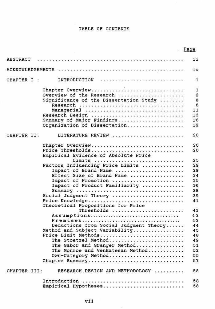
TABLE OF CONTENTS

ABSTRACT ii

ACKNOWLEDGEMENTS iv

CHAPTER I :

CHAPTER II:

CHAPTER III:

INTRODUCTION 1

Chapter Overview. . . . . . . . . . . . . . . . . . . . . . . . . . . . . . . 1 Overview of the Research . . . . . . . . . . . . . . . . . . . . . . 2 Significance of the Dissertation Study........ 8

Research . . . . . . . . . . . . . . . . . . . . . . . . . . . . . . . . . . . 8 Managerial . . . . . . . . . . . . . . . . . . . . . . . . . . . . . . . . . 11

Research Design . . . . . . . . . . . . . . . . . . . . . . . . . . . . . . . .13 Summary of Major Findings...................... 16 Organization of Dissertation................... 19

LITERATURE REVIEW ....................... . 20

Chapter Overview............................... 20 Price Thresholds......................... . . . . . . 20 Empirical Evidence of Absolute Price

Limits . . . . . . . . . . . . . . . . . . . . . . . . . . . . . . 25 Factors Influencing Price Limits . . . . . . . . . . . . . . 29

Impact of Brand Name . .. .. . . . . . . . . . . . . . . . .. . 29 Effect Size of Brand Name . . . . . . . . . . . . . . . . . . 34 Impact of Promotion........................ 35 Impact of Product Familiarity . . . . . . . . . . . . . . 36 Summary . . . . . . . . . . . . . . . . . . . . . . . . . . . . . . . . . . . . 3 8

Social Judgment Theory........................ 39 Price Knowledge................................ 41 Theoretical Propositions for Price

Thresho 1 ds . . . . . . . . . . . . . . . . . . . . . . . . 4 3 Assumptions................................. 43 Premises.................................... 43 Deductions from Social Judgment Theory...... 44

Method and Subject Variability................. 45 Price Limit Methods............................ 48

The Stoetzel Method......................... 49 The Gabor and Granger Method................ 51 The Monroe and Venkatesan Method............ 52 Own-Category Method......................... 55

Chapter Summary. . . . . . . . . . . . . . . . . . . . . . . . . . . . . . . . 57

RESEARCH DESIGN AND METHODOLOGY ......... . 58

Introduction . . . . . . . . . . . . . . . . . . . . . . . . . . . . . . . . . . 58 Empirical Hypotheses........................... 58

vii

CHAPTER IV:

Experimental Design........................... 59 Independent Variable . . . . .. . . . . . . . . . . . . . . . . . . . . 62 Dependent Variables . . .. . . . . . . . . . . . . . . . . .. . .. . . 65 Methods . . . . . . . . . . . . . . . . . . . . . . . . . . . . . . . . . . . . . . . 65

Stoetzel Method . . . . . . . . . . . . . . . . . . . . . . . . . . . . 65 Own-Category Method . . . . . . . . . . . . . . . . . . . . . . . . 66 Method Validation.......................... 67

Products . . . . . . . . . . . . . . . . . . . . . . . . . . . . . . . . . . . . . . 70 Sampling . . . . . . . . . . . . . . . . . . . . . . . . . . . . . . . . . . . 72 Sample Size . . . . . . . . . . . . . . . . . . . . . . . . . . . . . . . . 73

Experimental Procedures . . . . . . . . . . . . . . . . . . . . . . . 74 Stage One/Pretest Of The Instrument............ 75 The Experiment/Phase One....................... 79

Stoetzel Procedure . . . . . . . . . . . . . . . . . . . . . . . . . 79 Own-Category Procedure . .. . . . . . . . . . . . . . . . .. . 80 Results of Experiment/Phase 1............... 83

The Experiment/Phase 2... .. . . . . . . . . . . . . . . . . . . . . 86 Stoetzel Procedure.......................... 86 Own-category Procedure . . . .. .. . . . . . .. .. . . .. . 86

Data Analysis..... . . . . . . . . . . . . . . . . . . . . . . . . . . . . . 87 Test-Retest Reliability..................... 88 Validity Coefficients. . . . . . . . . . . . . . . . . . . . . . . 88 Hypothesis Testing. . . . . . . . . . . . . . . . . . . . . . . . . . 90

Chapter Summary ............. . ). . . . . . . . . . . . . . . . . . 90 ,//"

RESULTS AND ANALYST$_:--..• -.. • ............... . 91

Preliminary Procedures......................... 91 Demand Artifacts......................... 91 Random Assignment ~o Groups.............. 92 Mortality Rate ... : . . . . . . . . . . . . . . . . . . . . . . . 93 Unusable Cases ..... ~..................... 93 Total Subject Participation.............. 95

Measuring the Price Thresholds................. 96 Stoetzel Method.......................... 96 Own-category Method ...... ~............... 97

Experimental Results........................... 97 Descriptive Statistics:.................. 97

Acceptable Price Range.............. 97 Lower Price Limit................... 101 Upper Price Limit ................... 104

Statistical Analysis........................... 105 Homogeneity of Variance Assumption

Results ...... '....................... 106 Two-Way Anovas and Non-Orthogonal

Designs............................. 110 Classical Experimental Approach ...... 111 Hierarchical Approach ................ 112 Classical Regression Approach ........ 112

Two-Way Analysis off Variance Results.......... 113 Full Data Results ........................ 126 Outlier Data Results..................... 127 Post-Hoc Tests........................... 128

viii

Hypothesis Testing ............................ . Price Threshold Change .................. .

Stoetzel Method Results ............. . Own-category Method Results ......... . Validity ............................ . V Construct

129 129 131 131 133 133 135 139

Reliability ......................... . Multimethod-Multitrait Results ...... .

Chapter Summary ............................... .

CHAPTER V: CONCLUSIONS ............................ 141 Study Overview ................................ 141 Discussion of Major Findings .................. 142 Significance of the Research . . . . . . . . . . . . . . . . . . 150 Limitations .................................... 154 Threats to Validity ............................ 155

Threats To Statistical Conclusions Validity.................................. 155

Low Statistical Power ................ 155 Statistical Assumptions.............. 155 Unequal Cell Sizes ................... 156 The Reliability of Measures.......... 157 Reliability of Treatment

Implementation................... 157 Random Irrelevancies in the

E~perimental Setting............. 158 Threats to Internal Validity .............. 159

Demand Artifacts..................... 159 Evaluation Apprehension .............. 160 History Effects ...................... 160 Maturation Effects ................... 160 Interactive Effect................... 161 Order Bias . . . . . . . . . . . . . . . . . . . . . . . . . . 161 Selection Bias....................... 162 Mortality Effects .................... 162

Effects of Extraneous Variability......... 163 Impact of Uncontrollable Variance.... 165

Stoetzel Results................ 165 Own-Category Results ............ 166

Future Research .......................... 168 Chapter Summary .......................... 170

REFERENCES. . . . . . . . . . . . . . . . . . . . . . . . . . . . . . . . . . . . . . . . . . . . . . . . . 1 71

APPENDICES:

A. Phase One Response Booklet: Stoetzel Method. . . . . . . . . . . . . . . . . . . . . . . 1 77

B. Phase One Response Booklet: Own-Category Method ................... 184

C. Phase Two Response Booklet: Stoetzel Method ....................... 192

D. Phase Two Response Booklet: Own-Category Method .................. 201

ix

E. Summary Frequency Results of the Instrument Pretests .................. 211

F. Summary Frequency Results of the Experimental Pretests/Posttests ...... 218

G. Group Means and Standard Deviations of the 2 by 2 Factorials . , ............. 231

H. Two-Way Analysis of Variance Fesults for Unbalanced Factorial Designs ......... 244

I. Analysis of Covariance Results . . . . . . . . . . . . 257

Vita........................................................ 264

x

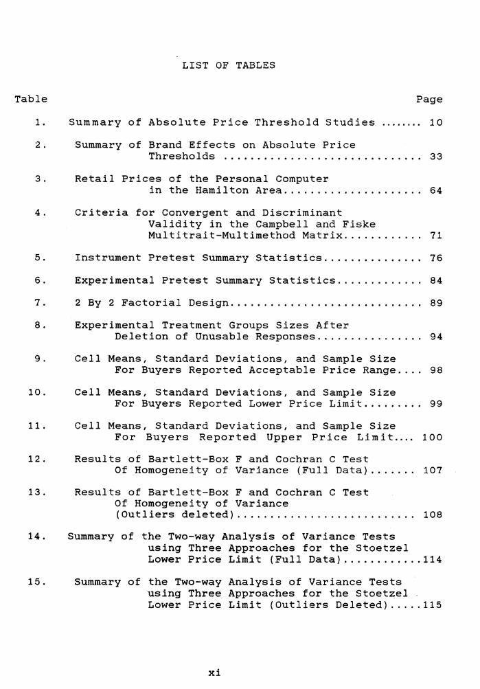
Table

1.

2 .

3.

4.

5.

6.

7.

8.

9.

10.

11.

12.

13.

14.

15.

LIST OF TABLES

Page

Summary of Absolute Price Threshold Studies ........ 10

Summary of Brand Effects on Absolute Price Thresholds . . . . . . . . . . . . . . . . . . . . . . . . . . . . . . 33

Retail Prices of the Personal Computer in the Hamilton Area ..................... 64

Criteria for Convergent and Discriminant Validity in the Campbell and Fiske Multitrait-Multimethod Matrix ............ 71

Instrument Pretest Summary Statistics ............... 76

Experimental Pretest Summary Statistics ............. 84

2 By 2 Factorial Design ............................. 89

Experimental Treatment Groups Sizes After Deletion of Unusable Responses ................ 94

Cell Means, Standard Deviations, and Sample Size For Buyers Reported Acceptable Price Range .... 98

Cell Means, Standard Deviations, and Sample Size For Buyers Reported Lower Price Limit ......... 99

Cell Means, Standard Deviations, and Sample Size For Buyers Reported Upper Price Limit .... 100

Results of Bartlett-Box F and Cochran c Test Of Homogeneity of Variance (Full Data) ....... 107

Results of Bartlett-Box F and Cochran C Test Of Homogeneity of Variance (Outliers deleted) ........................... 108

Summary of the Two-way Analysis of Variance Tests using Three Approaches for the Stoetzel Lower Price Limit (Full Data) ............ 114

Summary of the Two-way Analysis of Variance Tests using Three Approaches for the Stoetzel Lower Price Limit (Outliers Deleted) ..... 115

xi

16. Summary of the Two-way Analysis of Variance Tests using Three Approaches for the Stoetzel Upper Price Limit (Full Data) ........... 116

17. Summary of the Two-way Analysis of Variance Tests using Three Approaches for the Stoetzel Upper Price Limit (Outliers Deleted) .... 117

18. Summary of the Two-way Analysis of Variance Tests using Three Approaches for the Stoetzel Price Range (Full Data) ................. 118

19. Summary of the Two-way Analysis of Variance Tests using Three Approaches for the Stoetzel Price Range (Outliers Deleted) .......... 119

20. Summary of the Two-way Analysis of Variance Tests using Three Approaches for the Own-ca tegory Lower Price Limit (Full Data) ... 120

21. Summary of the Two-way Analysis of Variance Tests using Three Approaches for the Own-category Lower Price Limit (Outliers Deleted) ...................... 121

22. Summary of the Two-way Analysis of Variance Tests using Three Approaches for the Own-category Upper Price Limit (Full Data) .. 122

23. Summary of the Two-way Analysis of Variance Tests using Three Approaches for the Own-ca tegory Upper Price Limit (Outliers Deleted) ....................... 123

24. Summary of the Two-way Analysis of Variance Tests using Three Approaches for the Own-category Price Range (Full Data) ......... 124

25. Summary of the Two-way Analysis of Variance Tests using Three Approaches for the Own-category Price Range (Outliers Deleted) .. 125

26. Paired T-test Results ............................... 130

27. Multitrait-Multimethod Product Moment Correlations .............................. 134

28. Pearson Product Moment Correlations and the Criteria for Convergent and Discrimiant Validity: Multitrait-Multimethod Matrix (Three Traits and Two Methods) .......... 137

xii

29. Effects of Market Price Inforamtion on the Price Range, Lower Price Limit, and Upper Price Limit ............................ 146

xiii

FIGURE

1.

LIST OF FIGURES

Distribution of Maximum and Minimum Prices for Four Prcducts/Gausso-logarithmic co-ordinates

Page

31

2. Solomon Four-Group Design ......................... 60

3. Multitrait-Multimethod Matrix for Three Traits and Two Methods .................... 63

xiv

CHAPTER I

INTRODUCTION

This dissertation examined the effect of market price

knowledge on buyers' acceptable price range, and explored the

effect of market price knowledge on the lower and upper price

thresholds (limits). In addition, the construct validity of two

price threshold measures were assessed in terms of convergent and

discriminant validity through the multitrait-multimethod

procedure.

CHAPTER OVERVIEW

This chapter briefly introduces the theoretical foundation

for the existence of absolute price thresholds, and introduces

four methods that have been used to measure the absolute price

threshold concept. Moreover, the importance of this research in

terms of furthering marketing knowledge from both a theoretical

and practical standpoint is discussed.

A general overview of the factors that impact on price

thresholds is outlined, and the research plan to test the effect

of market price knowledge on the absolute price thresholds is

delineated.

The chapter concludes with a summary of the major findings

of the research and presents an outline of the organization of

the dissertation.

1

2

OVERVIEW OF THE RESEARCH

The theoretical foundation for the existence of absolute

price thresholds has been analogically derived from Weber-

Fechner's law, and psychophysics (Webb 1961). Psychophysics

deals with determining individual sensitivity to physical stimuli

or the nature of the relationship between physical and

psychological stimuli (Corso 1963). It has been established that

humans have upper and lower limits of responsiveness to physical

stimuli where these limits are referred to as upper and lower

absolute thresholds (Monroe 1973). For example, the reader is

probably familiar with hearing and eye examinations. In the

former case there are sounds at the high and low octave level

that the listener can no longer hear. The high and low octave

sounds that the listener can barely hear are called the

listener's upper and lower absolute hearing thresholds. These

thresholds then mark the transition between responsiveness and

non-responsiveness to a stimulus.

Since price is a physical stimulus, buyers should have

absolute upper and lower price thresholds. Absolute price

thresholds are defined as thresholds that mark the transition

between response and non-response to a price stimulus (Monroe

1973). The absolute upper price threshold is the maximium price

that a buyer would be willing to pay for a product. The absolute

lower price threshold is the minimium price a buyer would be

willing to pay for a product. (The terms price thresholds and

price limits are identical and w~ll be used hereinafter

3

interchangeably).

Based on psychophysics, individuals contemplating a purchase

should have an absolute lower price threshold (usually above $0)

and an absolute upper price threshold relative to the product

offering. Price offerings that fall within a subject's absolute

price thresholds are perceived by the buyer as acceptable and may

prompt the purchase of the product. Prices that are below the

buyer's absolute lower or above the absolute upper price

thresholds would be considered unacceptable, and a purchase would

be less likely to be made. Therefore, there are prices that a

buyer would consider too low (usually above $0) or too high for a

product and would not consider purchasing the product when price

is an important purchase determinant (Monroe 1971, 1979).

The existence of absolute price thresholds has been

investigated and confirmed by several researchers using various

methods (Monroe 1973;Raju 1977). However, little is known about

the factors that affect absolute price thresholds, and,

concomitantly, the acceptable price range (Raju 1977). Any

discussion concerning absolute price thresholds cannot be

divorced from alluding to the acceptable price range which is

defined as a range of acceptable prices that are bounded at the

extremes by the absolute lower and upper price limits.

From the two studies conducted in the area of acceptable

price range change (Fouilhe 1960; Raju 1977), subjects' product

price knowledge and product price categorization have been

mentioned as possible factors influencing absolute price

thresholds and acceptable price ranges. Price knowledge is

4

defined as the amount of price information that a buyer brings

into a purchase situation (based on consumer purchase behavioral

models in term.s of the search for information). Price level or

price categorization refers to the classification of a product in

terms of the perceived cost to the buyer (e.g., low priced,

medium priced, high priced product).

Four methods have been used to measure absolute price

thresholds: (1) the Stoetzel method (1954), (2) the Gabor and

Granger method (1966), (3) the Monroe and Venkatesan method

(1969), and (') the Own-category method (Sherif 1963: Monroe

1971). However, none of these methods have been shown to yield

empirically reliable or valid measures of absolute price

thresholds.

The purposes of this dissertation were: (1) to determine if

market price knowledge affects the acceptable price range, and

concomitantly, the absolute price thresholds, and ( 2) to assess

the convergent and discriminant validity of two different

research methods.

The two methods used in this study were selected on the

basis of a scientific criterion for assessing construct validity.

Construct validity is defined as the construct, trait, or concept

that the measure(s) is (are) in fact measuring. Construct

validity should be measured by at least two maximally different

methods, othe:rwise the researcher has no way of knowing whether

the construct or trait is anything but an artifact of the

measurement procedure (Peter 1979:Churchill 1979). Moreover, as

5

detailed in Chapter III, two criteria for establishing construct

validity must be assessed: (1) convergent validity, and (2)

discriminant validity. Convergent validity is the degree to

which two or more attempts to measure the same concept through

maximally different methods are in agreement; discriminant

validity is the degree to which a concept differs from other

concepts (Churchill 1979; Campbell and Fiske 1959; Bagozzi 1980).

As detailed below, the Stoetzel method ( 1954) and the Own-

category method (Monroe 1971) were considered different research

methods. The Stoetzel method (1954) is simple in application.

The method makes use of some variation of two questions:

(1) "Below what price would you suspect that this product was of

poor quality?"

(2) "Above what price would you judge this product to be too

dear?"

·Gabor and Granger (1966) and Monroe (1971) have criticized

this method on a number of grounds. First, the method uses

leading questions. Second,the term "dear" is ambiguous. Third,

the method does not allow for inferences to be made concerning a

subject's purchase intention. Subjects are asked only to name a

price but not in terms of their willingness to buy. While these

criticisms may be justified, the question remains whether the

criticisms make a difference in price threshold measurement.

Moreover, the criticism of the ambiguity of the term "dear" could

be considered specious. It reflects the arbitrary selection of

the proper English translation of the French term "Cher." The

6

translation and interpretation of the term is an artifact of

cultural differences. The term "Cher" can be translated into

English as either "dear" or "too expensive." In the original

translation of the Stoetzel {1954) work that appears in Taylor

and Wills (1970) the term "cher" is translated as "dear", but

researchers who have used the Stoetzel method modified the method

to reflect their cultural environment (Raju 1977; Deering and

Jacoby 1972). In these studies the term "cher" is replaced with

the phrase "beyond which it would not be worth paying more." This

phrase is one def ini ti on for the term "too expensive." Nonethe-

less, whether the Stoetzel method is a valid measure of absolute

price thresholds cannot be determined until it is empirically

tested against other methods purporting to measure the price

threshold construct.

The Monroe and Venkatesan (1969) method utilizes two methods

adapted from psychophysics, and the Own-category method (Sherif

1963; Monroe 1971) has been adapted from social judgment theory

(Sherif and Hovland 1961; Sherif, et al. 1965). Both of these

methods are complex in application and are more time consuming

vis-a-vis the Stoetzel method. However, both of these methods

improve upon the Stoetzel method. Neither method uses leading

questions nor purports to use ambiguous terms. The methods

establish absolute price thresholds in the context of a subject's

willingness to buy.

The Monroe and Venkatesan method, and the Own-category

method do differ in their intended aims. The Monroe and

7

Venkatesan method makes use of two psychophysical methods: (1)

the method of limits, and (2) the method of constant stimuli.

These psychophysical methods were developed to measure

"objective" responses to stimuli where the stimuli are unknown to

the subject. However, for price threshold measurement, the price

stimulus is known to the subject, and subject response to price

is "subjective." As a result, the Own-category method is

considered more appropriate for measuring absolute price

thresholds. The Own-category method was developed for the

purpose of quantitatively measuring "subjective" responses to

stimuli (Monroe 1971). Despite the difference in method purpose,

Monroe (1971) experimentally compared the price thresholds

measured by the two methods and concluded that the two methods

did not produce different results in the price limits using

different samples measured only a few weeks apart. The author

presented no statistical support for the above assertion.

The Gabor and Granger (1966) method also improves upon the

Stoetzel (1954) method by eliminating the leading questions and

allows for inferences to be made about a subject's willingness

to buy. In their method the subject is asked to respond to

different prices called out to them, by saying either "Buy", or

"No, too expensive," or "No, too cheap." This method is simple

in applicatio·n. However, the Gabor and Granger (1966) method is

only a slight modification of the Stoetzel (1954) method. It

allows inferences to be made about willingness to buy at any

stated price. By rephrasing the Stoetzel (1954) questions to

include willingness to buy, the two methods would seem to be

8

similar.

Overall, the four methods for measuring absolute price

thresholds can be classified into two groups based on similarity

and complexity of application. The Monroe and Venkatesan (1969)

method and the Own-category (1971) method are complex in

application, but have been asserted to yield similar absolute

price threshold scores in a single instance. The Stoetzel (1954)

method and the Gabor and Granger (1966) method are simple in

application and differ only in that the latter method allows for

willingness to buy inferences to be made. However, there is

little difference between the two methods if the Stoetzel

method's two questions are reworded to incorporate the inference

to willingness to buy. As a result of this classification, the

Stoetzel (1954) method and the Own-category (Sherif 1963; Monroe

1971) method were selected.

SIGNIFICANCE OP THE DISSERTATION STUDY

Research

Marketing researchers have been criticized for their failure

to develop valid measures for the constructs that they

investigate, and price researchers are no exception (Jacoby 1978;

Churchill 1979; Peter 1981). Therefore, one of the major

concerns facing researchers dealing with the measurement of the

absolute price threshold concept is to determine whether their

method(s) actually measures the construct under investigation.

9

For example, Stoetzel ( 1954) questioned whether his method

measured the price threshold concept.

Of the 10 absolute price threshold studies (Table 1), none

has empirically validated the method(s) used in the study. By

validating an a~solute price threshold method(s), price

researchers investigating price .thresholds and acceptable price

range can make use of a method ( s) that has been shown to be val id

and, thereby, eliminate method artifact criticisms. Therefore, a

validation study assessing construct validity in terms of

convergent validity and discriminant validity would make a major

methodological contribution.

Stoetzel (1954), Adam (1958), and Gabor and Granger (1966)

have suggested that price thresholds may be affected by product

price knowledge and product price level. However, the effects of

these two factors on the absolute price thresholds and acceptable

price range have not been investigated.

Two other factors that affect price thresholds and

acceptable price range have been studied. Fouilhe (1960)

investigated the effect of brand name on the acceptable price

range, and the mean maximium and the mean minimium price. Raju

(1977) assessed the effect of product familiarity (consumer

product expertise) on acceptable price range. Since both of

these methods used the often criticized Stoetzel (1954) method,

it is not known whether the subjects, in fact, perceive "too

dear" or "poor quality." Therefore, the results can be

criticized due to face validity of the measure.

0 ....

TABLE 1

SUMMARY OF ABSOLUTE PRICE THRESHOLD STUDIES STtlnY MnHoos 1 rii0n11cTs - 1 i.owu 1 uPPu 1 acci,.n 11L11 p110011cn 1 11uHo 11aME I Flioouct I uauoet 1

llS!D I I PlllC! I PlllC! I PRICK I PllYSICALLT I Pll!S!MT I FAMILJAlllTT I PlllCE . I I I LIMIT I LIMIT I llANOS I Pll!SEMT!D I I MEASURED I KllOlfLEDOE I I I I I I I I I

------'----'------1---1 I I I I 1------stoetnl I lltoHtel lhdlo I fHDO I fHOOO I IHOO I llo I ,.. I llo I llo 1191111 I I I I I I -- '-------' '----' '- , _____ _ Ad.. I 9toetael fStocltlnv• I ruo I 11000 I ueo-, I 19HI I f91lp• I nt• I nt• I nta I

I fSho•o I nte I nl• I nl• I fOeo Lloht•r I n/a I n/• I n/a I fOold-Notch I n/• I nl• I n/o I fllefrloerotor I n/o I n/• I n/a

---- 1 _____ 1 I 1---FouJJh• I Stoetzel (8r•nd•d I 19501 I flloohlng P.....Ser 1111

I f llnbrondod I 111 .. hlng Powder ne I IBrend•d I I Peck•oe Soup no I f llnbr•nd•d I I Peck•o• Soup ru

-------'-----'-Gabor •nd I Stoetzel/ JStocklno• I nt• Or•no•r I O•bor 6 JC•rp@t I nl• I 1966 I I Oronper I Pood I I n/•

I 1rooc1 2 I n/o I fllouH Article 1 I n/• I fRouee Article 21 n/•

------'-----' '----· Gebor and I Stoet2el/ fStocklnoo I n/• I Grongn I O•bor a fcarpet I n/• I I 1910) I Orenoer I rood I I n/• I

I 1 rooc1 2 I nto I I fllouH r.rtlclo 1 I n/o I I fHouH Artlc'lo 21 n/• I

rno flll

1130

ruo n/• n/• n/• n/• nt• n/o

n/• n/o n/a n/• n/• n/•

fll

uo uo rae nl• nl• n/• nl• n/e n/o

n/e n/• n/o n/• n/o nt•

••• y .. , .. Ye• 110 No

Yee

Ye•

, .. , .. llo Y•• 110 llo llo No

llo h• llo llo No llo

--------'-----'- I I I '------Sherif IDwn-CoteooryfNlnter coot I I 11953) I I Jndlen I 912.15 I ,,,_,g

I I llhlte I UD.51 I 131.95 111.11 Ul.05

llo

I I I I ---- 1 __ ··--- -'------·-----·--... --------'----' 1 _____ _ Honroe and I Honroe 6 f8Jouce I Sl. 10 I . ti. JO I tO .. •o I llo Venk•t•••n 11969)

I Venkoteeon fDre•• Shirt I 99.DO I 919.10 I 910.IOI llo I I 11• 1 r Sprey I to. 59 I ti . 11 I ti . 29 I No I fHelr Dryer I 913.19 I 923.30 I 99.101 ·110 I fatter-Shove I Sl.15 I 93.31 I fl.151 I iOreoe Shirt I $3.U I u.ao I ,,_,,, I l!loctrlc Shover! UJ.15 I tU.10 I U-151 • I fSporte ci>et I tU.15 I 951.16 I 921.0JI

-------'-----1--------'----'---1 I Monroe I Monroe 6 fDre•• Shoee I 99.00 I .tit.JO I 910.IOI 11911) I Venketeeon ISporte Cnot I 924.1& I 951.75 I 921.011

I I I I I I fOWn-CetegoryfDreee Shoe• I Sl.15 I tl9.1D I tll.001 I fSporte Coet I UI .50 I 949.DO I 9'8.oor _____ , ________ , ________ , _____ 1 ___ , ____ 1

Downey 10wn-cote9oryfrente I I I I I nnJ I I I I I I

I 111010 I 9s.50 I 919.oo I tu.101 I fFeulee I $6.no I 919.00 I 913.001 ________ , ________ , ___________ , _______ 1 ___ , _____ 1

r-."'Ju I Stoetzel ISt~rC!o flecelv~rl I I I 119711 I IHI lnvolv••ent I 9216.66 I 9291.66 I '7~.0~1

I p.nw tnvoJvtt .. ~nt I SICI0.62 I $2ftl.!t0 I 9~f;.1181 I I ' t I I

No llo llo llo

llo lfo

No

No

llo llo llo llo No llo

y ..

TH

Yee

, .. llo llo llo llo llo llo

llo No llo llo llo llo

llo

llo No No llo llo llo llo llo

No llo No

110 llo llo llo 110 No

llo

llo

llo

110

No llo llo llo No llo

llo llo llo llo llo llo

llo

110 110 110 No No llo llo llo

llo llo llo

'-----No ' I I I

Ho

-----'-----1 No I Yeo I I ! !

llo llo llo llo llo llo

110

llo

llo

llo

110 llo llo llo llo 110

llo llo No llo 110 llo

llo

No llo No No llo llo No llo

llo No No

--ii()--, I I

I I , ________ I I Nn I I I ! !

11

Raju (1977) underscores the importance of acceptable price

range research by claiming that a systematic investigation of

acceptable price ranges is particularily important because price

variations within the unacceptable low, acceptable, and

unacceptable high ranges might have different effects on

perception and evaluation of products. Moreover, Petroshius

(1983, p.160) suggests that any research manipulating a price

range with the intent of representing a subjects' acceptable

price range (and absolute price thresholds) would require the

"development of more precise and effective means of measuring and

manipulating" the subjects' acceptable price range. The validity

of different methods of determining buyers' acceptable price

ranges should also be a focus of future research. However,

before .such research can be undertaken, absolute price thresholds

and acceptable price range measurement must be better understood.

The effect of differences in market price knowledge on

absolute price thresholds and acceptable price range will provide

price researchers with a better substantive understanding

concerning how absolute price thresholds and acceptable price

ranges differ across situations. Moreover, such research leads

to the initial development of a general absolute price threshold

and acceptable price range theory.

Managerial

Developing an appropriate pricing strategy for a firm's

product(s) or product line(s) is a complex and an important

decision. The pricing decision affects the firm's revenues

12

directly and costs indirectly. Moreover, the pricing decision

has been exacerbated by the prevailing environmental forces.

Increased foreign competition, raw-material shortages, increasing

labor and material cost, high interest rates, decreasing

corporate liquidity, and a recessionary cycle have made product

pricing more important than ever. As a result of these forces,

the firm has found itself in an environment where pricing a

product incorrectly may have a pronounced effect on sales and

profits.

The pricing practices of most firms focus on product costs in

setting the price of a product. But product cost plays a limited

role in the pricing decision (Monroe 1979). While the cost

variable indicates whether the product can be sold at a prof it at

any price, it does not indicate the price the buyer will accept.

As such, product costs set the lower limit to the pricing

decision. The upper limit, however, is determined by demand, the

buyers' willingness to purchase the product at the stated price.

Therefore, a better understanding of absolute price thresholds

and the acceptable price range concept can help to reduce pricing

errors, not only for new products, but for products already on

the market where price increases or decreases are managerial

options. Acceptable price thresholds provide the manager with a

relatively easy way to determine the range of prices a firm

should consider setting for a given product. Moreover, because

inferences can be made between price and willingness to buy, a

manager can determine the percentage of potential buyers at any

given price within the acceptable price range (Gabor and Granger

13

1966, 1970).

When factors that influence the acceptable price range (and

by definition. price limits) are better understood, then marketers

can price their products more accurately within consumers' price

limits to insure consumers' willingness to buy. Moreover, where

firms have similar products with different features at different

prices to appeal to different markets, then it may be possible to

determine the acceptable price ranges existing in each segment.

Price perceptions and product evaluation may differ for

different market segments (Monroe 1971; Petroshius 1983).

Information on factors that affect absolute price thresholds and

acceptable price range would provide marketers with information

to modify their marketing program to further enhance the

likelihood of their target consumers purchasing their brands.

Research Design

The procedure used in this research was a laboratory

experiment with a series of 2 by 2 factorial designs based on the

Sol~mon four group - six study design. The dependent va~iables

are the absolute lower price limit, the absolute upper price

limit, and the acceptable price range. Market price information

was the experimental variable that was manipulated in this

dissertation. The market price information variable had two

treatment levels: (1) in the no or little market price

information treatment, subjects received no market price

information other than that present in memory, and (2) in the

market price information treatment, subjects were provided with a

14

table which provided the various prices that the product was

currently selling for in the local market place.

In the experimental treatment, a manipulation check was

conducted to insure that subjects had attended to the price

information provided. The manipulation check took the form of an

open-book exam based on a booklet containing the specific market

price information. Subjects were asked specific questions about

the market price information that was presented in the booklet.

Pretests and the manipulation check were conducted prior to the

actual treatment manipulation.

The Stoetzel (1954) method and the Own-category (1971)

method were used to measure the dependent variables. Moreover,

construct validity was assessed using Campbell and Fiske's (1959)

multitrait-multimethod methodology. This method provides a

multitrait-multimethod matrix, which is a matrix of zero-order

correlations between different traits when each of the traits is

measured by maximally different methods (Campbell and Fiske 1959;

Churchill 1979). The method is one way to assess construct

validity by investigating the pattern of correlations for

convergent and discriminant validity. These validities are the

cornerstone of construct validity (Campbell and Fiske 1959; Cook

and Campbell 1979; Bagozzi 1980; Peter 1981).

The experimental design used in this study for measuring the

effects of market price knowledge on price limits and acceptable

price range in a pretest/post-test situation was the Solomon

four-group design. The benefits of this design are six-fold

15

(Kerlinger 1973):

1) Reliability can be assessed due to the repeated measurement

design.

2) Randomized assignment of groups assumes statistical or

equivalent groups and allows for testing of homogeneity of

variances between groups.

3) History and maturation effects that affect internal validity

are more discernible.

4) Interactive effects are more discernible.

5) Evidence for possible temporary contemporaneous effects that

occurred between Time 1 and Time 2 can be obtained.

6) It provides the ability to

provides the power of

experiments.

test each group separately

replication because of the

and

two

The experimental design was statistically analyzed using a

series of 2 by 2 factorial designs, one for each of the dependent

variables for each of the two methods. This two-way anova design

has two factors. The first factor has two levels: pretest and no

pretest; the second factor also has two levels: absence and

presence of market price information. · The 2 by 2 factorial

design allows for the separate testing of each of the two main

effects and the interaction effect using F statistics. Paired t-

tests were used to assess the impact of market price information

on subject absolute price thresholds.

The test-retest reliability of the two methods for measuring

absolute price thresholds was assessed using Pearson's

16

correlation coefficient. Pearson correlation coefficients were

also calculated to set validity coefficients. The pattern of the

validity coefficients as outlined in Chapter III was examined to

assess construct validity in terms of convergent and discriminant

validity.

Summary of Major Findings

The basic hypothesis of this research study contends that

consumers' possess a range of acceptable prices that they are

willing to pay for a specific product, and that the acceptable

price ranges are reflective of the amount of market price

knowledge that consumers possess for a specific product. More

specifically, consumers who are exposed to market price

knowledge would be more discriminating and, therefore, would have

a narrower acceptable price range than those consumers possessing

little or no market price knowledge.

The experimental results partially confirmed the hypothesis

that student consumers adjusted their acceptable price range when

they acquired market price knowledge. The mean acceptable price

range was narrower for subjects who possessed market price

knowledge than when they possessed little or no price knowledge.

However, the empirical support for this finding was inconsistent

and was reflective of the method used to measure the acceptable

pr ice range.

The mean acceptable price range established for the subjects

when no price information was offered did, indeed, changed after

17

the subjects were presented with market price information. The

mean acceptable price range was significantly narrower after the

subjects were presented with market price information when the

Stoetzel Method was used. However, when the acceptable price

range was calculated using the Own-category procedure no change

occurred due to the introduction of market price knowledge.

Moreover, the acceptable price range moved upward to reflect the

market price knowledge. That is, the lower and upper price limit

increased with the introduction of market price information with

the Stoetzel method, but only the lower limit increased with the

Own-category method.

The lower price limit for both methods was higher for those

subjects who were provided market price information than those

who were not. However, the upper price thresholds for. both

methods revealed no change in the price thresholds due to market

price information when the analysis was conducted on the full

data. However, when outliers were deleted from the data, the

upper price threshold scores were greater for subjects who

received market price information when subjects used the Stoetzel

method. But, there was no change in the upper price threshold

scores for the Own-category method due tb the treatment. Subjects

receiving market price information had narrower acceptable price

ranges using the Stoetzel method but not with the Own-category

method. Primarily, the Own-category method produced more

variability in the upper price threshold than did the Stoetzel

method, thus indicating a major difference in the methods at

least in terms of the upper price threshold. This finding would

18

suggest that future research should focus on investigating the

sources of the variability in the upper price limit.

Most importantly, the upper price threshold witnessed almost

twice the variability than the lower price threshold for both

methods. The variability in the upper price threshold was also

greater in the Own-category method than in the Stoetzel method.

However, this should not be an unexpected finding since the lower

limit is bounded by O but the upper limit is unbounded. As a

result, there is a higher probability of increased variance in

the upper limit. Nonetheless, this method variability most

certainly reduced the power of the testing procedure in the case

of the upper price threshold, as well as, the range of the

acceptable price range.

In hopes of reducing within-group variability and increasing

the power of the test procedures, post-hoc analysis of covariance

was conducted on the data using (1) sex of the subject, and (2)

prior price knowledge of the subject. The subsequent analyses

produced no change in the initial conclusions.

Based on the examination of the pattern of the validity

coefficients in the multitrait-multimethod matrix, both the

Stoetzel and Own-category method could be considered as valid

measures of the absolute price threshold concept. However, there

was greater measurement error in the Stoetzel method than in the

Own-category method. That is, the Own-category method produced

more reliable results than did the Stoetzel method.

19

Organization of the Dissertation

The dissertation is organized into five chapters. Chapter I

introduced the dissertation and presented a brief overview of the

study including the significant of the research for marketing

practice and knowledge, the research objectives, an outline of

the research procedure employed, and a statement of the major

findings. Chapter II develops the theoretical foundation of price

thresholds and acceptable price range. It reviews the literature

that provides empirical evidence for price thresholds, and

investigates factors that influence the acceptable price range.

Four methods for measuring price thresholds are critiqued. The

chapter concludes by proposing theoretical propositions derived

from social judgment theory consistent with the research

objectives. Chapter III outlines the research design and

methodology that was used to test the empirical propositions

introduced in Chapter II. Campbell and Fiske's multitrait-

multimethod method for assessing construct validity is detailed,

and reliability measurement is introduced. Finally, the internal

and statistical conclusion validity questions of the design are

presented, and the limitations of the methodology are detailed.

Chapter IV details the procedures used to analyze the data and

presents the results for each of the hypotheses. The dissertation

is concluded in Chapter V by discussing the study results,

limitations and contributions of the study, and suggests

directions for future research.

CHAPTER II

LITERATURE REVIEW

CHAPTER OVERVIEW

This chapter reviews the literature on the absolutu price

thresholds concept. The first section of this chapter introduces

the theoretical foundation of the price threshold concept, and

reviews the empiricial evidence supporting this concept.

The second section introduces two factors that may affect

price thresholds and, concomitantly, acceptable price range.

From the price threshold 1 i tera ture, brand name and buyer

expertise or product familiarity are introduced as factors that

may affect the absolute price limits and acceptable price range.

Moreover, product price knowledge and product price level are

alluded to as potential factors influencing the price thresholds.

Studies dealing with these factors are reviewed.

The third section deals with a comparative review of the

four price threshold methods that have hitherto been used as

appropriate measures for absolute price thresholds. The final

section presents the theoretical propositions derived from the

literature review.

PRICE THRESHOLDS

Perception is considered to be subject to thresholds of

awareness. From psychophysics, the study of quantitative

relationships between physical objects and psychological events,

researchers have found that there are absolute upper and absolute

20

21

lower boundaries to human perceptual and sensory capabilities

(Monroe 1973, 1979).

The theoretical justification concerning the existence of

absolute thresholds in price perception has been analogically

derived from Weber-Fechner's law and the p1·inciples of

psychophysics (Webb 1961). From this perspective, absolute price

thresholds are viewed as limits of responsiveness to extreme

price stimuli in much the same way as sensory limits of

responsiveness have limits of responsiveness to extreme sensory

stimuli (Monroe 1973, 1979; Gardner 1977).

In their comprehensive review of psychological pricing

literature, Monroe (1973), and Monroe and Petroshius (1981)

suggest that an understanding of buyer response to price must

consider a buyer's price thresholds. Empirical studies have

indicated that every human sensory process has an upper and lower

limit of responsiveness. These absolute thresholds then mark the

transition between response and non-response to a stimulus. If we

consider price to be a stimulus, then ~ E~i2~i there should be

upper and lower price limits for a contemplated purchase. That

is, a product priced above a potential buyer's absolute upper

price threshold, or below the absolute lower price threshold

would be less likely to produce a a willingness to purchase

response. Translating this phenomenon into consumer

interpretation of price leads to the hypothesis that there are

prices below and above which buyers will consider the price

inappropriate and may not purchase. Moreover, buyers

contemplating a purchase enter the market not with a single price

22

in mind they are willing to pay, but with a range of acceptable

prices bounded by lower and upper price limits.

The rationale for the lower 1 imi t seems to be in the buyers 1

suspiciousness of 11 too good a deal" and the feeling that "you get

what you pay for 11 (Stoetzel 1954; Adam 1958; Fouilhe 1960; Gabor

and Granger 1966). Consumers are believed to rationalize that

below a certain price quality is not trusted, while no brand can

be worth more than a certain upper price limit (Stoetzel 1954;

Gabor and Granger 1966, 1970). Therefore, certain prices may be

considered too low (usually above $0) or too high and would be

unacceptable to the buyer (Monroe 1971).

The theoretical foundation for the existence of absolute

upper and lower price thresholds is based on a modification of

Weber's Law --- Weber-Fechner•s law ( Monroe 1973) which is given

as:

R = k log S + a

where R is the magnitude of response,

S is the magnitude of the stimulus,

k is the constant of proportionality,

a is the constant of integration.

Weber-Fechner's law in psychophysics provides predictions

concerning some properties of the absolute price thresholds.

Simply stated this law establishes a logarithmic relationship

between the magnitude of the stimulus and the magnitude of a

response where consumers are more sensitive to price stimuli at

23

the extreme of their price limits (Monroe 1973; Monroe and

Petroshius 1981). In the context of price perception, the law

produces the hypothesis that the relationship between price and

an operationally defined response (e.g., willingness to buy) is

logarithmic (Monroe 1973). Moreover, Weber-Fechner's law

provides a means of quantifying absolute price thresholds because

a least squares regression relating R to log Scan befitted from

the data. The price thresholds are then operationalized when a

subject can perceive a stimulus (price offering) value fifty

percent of the time (Corso 1963; Monroe 1971). The price

threshold limit is ~!~!£!1Y defined as the point at which 50

percent consider the price offering as acceptable to pay and 50

percent that consider unacceptable to pay (Monroe and Venkatesan

1969; Monroe 1971; Sherif 1963; based on Corso 1963). It should

be emphasized that one is referring to one subject and not an

aggregate of subjects; i.e., it is the price value that maximizes

indecision for one person.

The argument for price thresholds is based on psychophysics

and a discussion of perception to justify lower and upper price

limits. However, price limits are defined in terms of attitude;

i.e., purchase intention. This is not a perceptual variable. As a

result, a direct translation to price perception is that given a

range of price stimuli, some of those prices are not perceived.

It was not until the research of Sherif (1963) and Monroe

(1971), that social-judgment theory was offered as a theoretical

explanation for the existence of price thresholds and acceptable

price ranges.

24

Latitudes of acceptance and rejection, and involvement are

concepts central to social-judgment theory developed by Sherif

and Hovland (1961) and revised by Sherif et al. (1965), and

Hovland et al. (1953) in assessing shift in individual judgments

of stimuli. According to this theory, a person's interpretation

of a pyschological judgment scale is predicated not on a single

position but rather determined by a band of acceptable positions

--- or a latitude of acceptance. The opposite concept, the

latitude of rejection, includes all those elements that an

individual finds unacceptable. The theory posits that individuals

evaluate stimuli based upon a preexisting psychological judgment

scale. This internal scale is comprised of three distinctive

segments referred to as latitudes of acceptance, rejection, and

noncommitment. Each latitude encompasses a range of stimuli.

In the context of pricing, latitude of acceptance would

constitute an acceptable price range, latitude of rejection would

translate as an unacceptable price range, and latitude of

noncommitment would consist of a range of neither acceptable nor

unacceptable prices. The key point is that the regions are

derived from a judgment process that combines an evaluation and

comparison of all the objects in the stimulus set (Sherif et al.

1965). By price judgment is meant the individual's assessment of

whether a price is too low (unacceptable low), just right

(acceptable), or too high (unacceptable high).

The logical process would entail a price assessment or

judgment in terms of purchase intention. The lower price limit

25

implies "cheap" and cheap implies "poor value" for the money and

poor value implies "don't buy." The same type of logical

inference can be made for the upper price limit. A high price

implies "too expensive" and too expensive implies "poor valU(!"

for the money and poor value implies "don't buy."

EMPIRICAL EVIDENCE OP ABSOLUTE PRICE LIMITS

The notion that buyers have a range of acceptable prices

that are bounded at the lower and upper limits they are willing

to pay has been confirmed using both survey and experimental

methodologies over a range of differently priced products

(Stoetzel 1954; Adam 1958; Fouilhe 1960; Gabor and Granger 1966,

1970; Sherif 1963; Monroe 1971; Monroe and Venkatesan 1969; Raju

1977; Downey 1973).

Stoetzel (1954) was the first to report the existence of a

range of prices buyers are willing to pay for a radio. Stoetzel's

work was reinforced by a fellow Frenchman, Adam (1958).

Interviewing 6,000 subjects, he determined price limits for nylon

stockings, an underwear item, children's shoes, men's dress

shirts, a gas lighter, and refrigerators. Unlike Stoetzel

(1954), Adam physically exposed the respondents to the four

"clothing items to the respondents. Table 1 provides the actual

price limits and acceptable price range for the products used in

each of the 10 studies. Unfortunately,

the data provided by the studies

it was not possible given

to determine if findings

differed under various testing conditions (e.g., product

present/absent, method differences, product type, etc.). In some

26

studies, the price limits were not reported or no data were

provided from which the price limits could be calculated.

However, where a comparison can be made to bring insight to the

issues, they are presented in the analysis.

Fouilhe (1960) also established price limits for a laundry

detergent and a package soup. Furthermore, Fouilhe expanded the

procedure to include not only exposure to the products

themselves, but added brand name for each of the two products.

Raju (1977) established price limits for a stereo receiver

without physically presenting the product to the respondents.

Product familiarity in terms of buyer expertise was incorporated

into his methodology.

In their series of studies, Gabor and Granger (1966, 1970)

confirmed the existence of price limits for several food

products, two categories of non-durable household articles, nylon

stockings and carpet. The 6,000 subjects were able to physically

examine only the carpet, and the data were identical in each of

the studies. That is, data were gathered for the initial study

(Gabor and Granger 1966) and the same data were presented but

analyzed differently in each study.

Sherif (1963) identified value series (acceptable price

limits) for a winter coat from among 334 high school students,

using an experimental method based on social judgment theory.

Monroe (1971) replicated Sherif's study using high school

students and established price limits for women's dress shoes and

a man's sports coat. The importance of this study is not so much

that the study replicated the Sherif (1963) results, but that the

27

study was the first to utilize and empirically compare the price

limit scores from more than one experimental method. The

acceptable price limits determined by the method of limits/method

of constant stimuli and the Own-category method were found not to

be significantly different despite the fact that the intended

measurement purposes of the two methods differed. Moreover, the

results were not found to be statistically different even though

data were collected from two different samples (college and high

school students} and that only a few weeks separated the two

studies.

The psychophysical method makes use of two methods, the

method of limits and the method of constant stimuli. These

methods were developed to measure responses to physical stimuli,

where the magnitude of the stimuli are unknown to the subject.

However in pricing experiments, there is no way to hide the

magnitude of the price stimulus. A subject categorizing a price

as acceptable or unacceptable is assumed to be reacting to the

price variable relative to an entire set of purchase decision

variables. Thus, the subject's reaction to price is subjective

(Monroe and Venkatesan 1969; Monroe 1971). As a result, the Own-

category method is considered a more appropriate method for

measuring price thresholds. The Own-category method was

specifically developed to establish a measurement scale where the

underlying judgments are subjective in nature.

Monroe and Venkatesan (1969) determined acceptable price

limits for a number of clothing and personal care items for

28

college students. This study introduced a new method for

measuring acceptable price limits. They adapted psychophysical

experimental methodology (method of limits/method of constant

stimuli) and confirmed the acceptable price limit hypothesis.

D0wney (1973) and Cox (1986) used the Own-category method to

establish acceptable price thresholds among college students for

pants.

In sum, the absolute price thresholds concept has

theoretical foundation and has been supported empirically across

a number of products using various methods. From a managerial

point of view, the price-limit hypothesis has important

implications for demand estimation, new product pricing, and

product line pricing. The most important implication of the

price-limit hypothesis is the need to place more emphasis on

demand as a price-decision determinant (Monroe 1971; Petroshius

1983) .

Despite the importance of the absolute price threshold

concept, little attention has been paid to factors that may

influence these thresholds. An investigation into the factors

that influence price thresholds is particularly important for

theory development. As Monroe and Venkatesan (1969) point out,

the research on price thresholds is embryonic since information

normally available to consumers such as price knowledge, brand

name, store image, etc. fil~Y lead to variability in absolute

price limit and acceptable price range measurement. By

identifying factors that affect absolute price limits, marketing

managers can determine more accurately the price limits and

29

acceptable price ranges for products from which they can set

product prices. Setting a product's price from prices within the

acceptable price range should promote a favorable evaluation of a

product at least in terms of the product's price.

From a theoretical perspective an investigation into factors

that affect absolute price thresholds can be seen as an initial

attempt to develop a general absolute price threshold theory.

Therefore, this dissertation was primarily concerned with

addressing two questions: ( 1) does market price knowledge

influence the acceptable price range; and (2) do the various

measures of price limits and acceptable price range produce

different price limit scores? A secondary concern was to

determine the effect of market price information on the absolute

price thresholds from which the acceptable price range is

determined.

In the next section, some potential infuential factors that

have been found to affect price thresholds are identified. Also,

the methods that have hitherto been used to measure absolute

price thresholds will be outlined.

FACTORs IHFLUEHCIRG PRICE LIMITS

Impact of Brand Bame

Only the studies conducted by Fouilhe (1960) and Raju (1977)

investigated factors that may affect price limits and

subsequently, acceptable price ranges. Fouilhe (1960) expanded

the Stoetzel (1954) methodology by including not only exposure to

30

the products, but also brand name for each of the two products.

Using the Stoetzel (1954) method, he reported three findings. (1)

Branded products had a narrower acceptable price range than their

corresponding unbranded products. (2) The mean maximum and mean

minimum price {upper and lower price limits) of the branded

laundry detergent product were found to be statistically

different due to promotional stimulus. And (3) the mean maximum

price {upper price limit), but not the mean minimum price (lower

price limit) was found to differ across all products due to the

age of the respondents. That is, the mean maximum acceptable

price increased as the age of the respondents decreased. This

last finding could suggest that the more experienced the buyer,

and consequently, the more knowledgeable the buyer, the lower the

maximum mean acceptable price.

A closer investigation of the results reported contradicts

the first contention. No statistical evidence was provided to

support the contention that the price ranges for the

branded/unbranded products differed. Based on the distribution

of the maximum and minimum prices for the products provided in

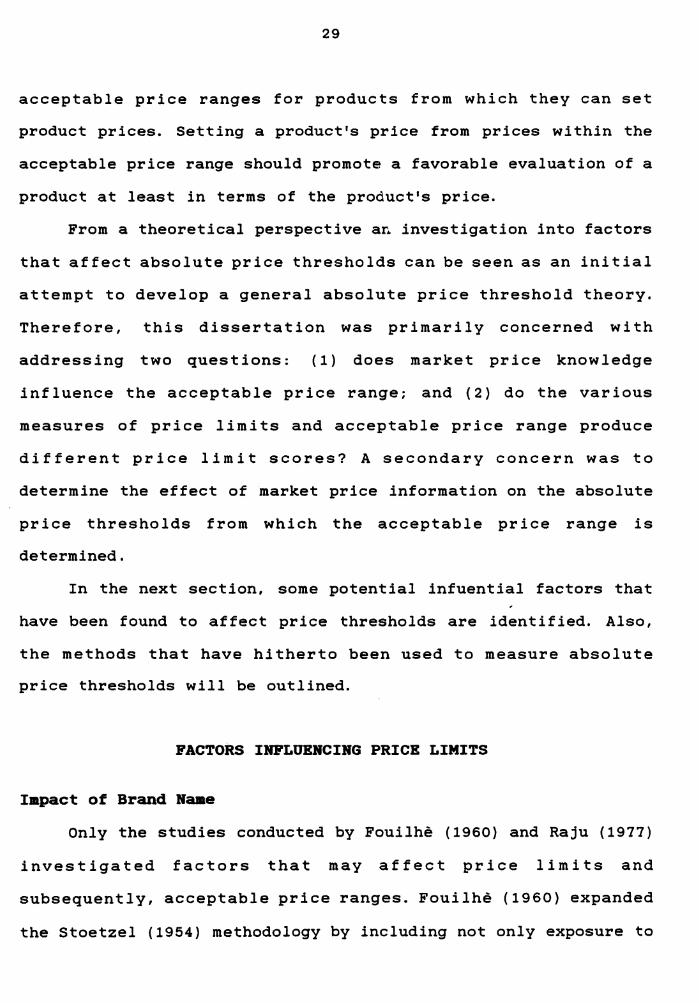
the study on a Gausso-logarithmic graph and reproduced in Figure

1, the acceptable price range was narrower for the branded

package soup but not for the branded laundry detergent vis-a-vis

their unbranded counterpart. The acceptable price range for

unbranded package soup was 55 French francs, and for the branded

soup it was 40 French francs. The acceptable price range for the

branded laundry detergent was 75 French francs and for the

Unbranded Laundry Detergent

Unbranded Packaged Soup

50 100 200 400 francs

31

FIGURE 1

Branded Laundry Detergent

50 100 200 400 francs

Branded Packaged Soup

50 1 00 200 400 francs

DISTRIBUTION OF MAXIMUM AND MINIMUM PRICES FOR FOUR PRODUCTS

GOSSO-LOGARITHMIC CO-ORDINATES

32

unbranded detergent it was 40 French Francs. (It should be noted

here, however, that this interpretation was based on calculating

the absolute differences in price ranges from the data provided

in the study because it was not possible to statistically retest

the assertion due to the dearth of appropriate statistics).

Based on these findings detailed in Table 2, it would seem

that brand name does impact on the acceptable price range at

least in absolute terms. For some products, the introduction of

brand name narrows the acceptable price range; for other

products, brand name causes the acceptable price range to widen.

However, no statisical evidence exists to indicate the extent of

brand influence on the acceptable price range.

The differences between the lower and upper price limits of

the unbranded/branded products were retested using the standard

deviations determined from the slopes of the minimum and maximum

acceptable prices presented. The standard deviation can easily

be determined from the Gausso-logarithmic graph provided in the

study since the standard deviation is proportional to the slopes

which represent the lower and upper price limits. The price

variable is entered directly on the abscissa and the cumulative

proportions are entered directly on the ordinal. The mean lies

at 0.50 (on a gausso-logarithmic graph the mean and median are

equal). The standard deviations of each limit can be calculated

by drawing a perpendicular line from the end of the slope to the

mean (Figure 1). In all cases the upper and lower limits vis-a-

vis unbranded/branded products were reported to be different at p

33

TABLE 2

SUMMARY OF BRAND EFFECTS ON ABSOLUTE PRICE THRESHOLDS

Product Treatment Lower Limit

Unbranded f75 Laundry I Detergent I Branded f115

I. I I Unbranded f65

Packaged I Soups I Branded f90

I

Product Treatment Upper Limit

Unbranded f115 Laundry Detergent Branded f190

Unbranded f120 Packaged Soups Branded f130

* I-----~--------"\

** t

r = I ------------\I t + DF

D 1---------"\ I DF

2 \I

Standard I Correlation t * I Effect•• Deviation I Lower Limit Value I Size "D"

l __ {l) __ I I I

f25 I I I 0.25 4.58 I 0.52

f65 I I I I I I

f20 I I I 0.38 7.27 I 0.82

f46 I I I I

Standard Correlation t * Effect** Deviation Upper Limit Value Size "D"

f75 0.34 6.43 0.72

f95

f40 0.43 8.43 0.95

f80 ----

t· value is the t statistic and is calculated from the correlation coefficient and degrees of freedom provided in the study.

The effect size "D" is calculated using the t Values.

(1) The correlations reported are the correlations of the lower limits and upper price thresholds for each of the branded/unbranded product combinations.

34

<0.05. Both the lower and upper price limits were higher for

the branded products than their nonbranded counterpart.

Effect Size of Brand Name

Effect sizes (D) or the effect of brand name on the price

limits were calculated for the products based on the formulas

provided by Rosenthal ( 1980) and are presented in Table 2.

Effect size (D) is defined as the difference between control and

treatment group averages, expressed in terms of the control

group's standard deviation (Pillemer and Light 1980).

The upper price limit for both branded products were on the

average almost one standard deviation (0.84) greater than the

upper price limit of their unbranded counterpart. Branded

products were on the average slightly more than one-half

standard deviation (0.53) greater on the lower price limit than

unbranded. However, the lower price limit effect on the branded

package soup was almost 58 percent greater than the effect on the

lower price limit of the branded laundry detergent ( 0.82, 0.52).

The upper price limit effect on branded package soup was 32

percent greater than the upper price limit effect on the branded

laundry detergent (0.92, 0.72). Since Fouilhe (1960) classifies

laundry detergent as a high-priced product, and package soup as a

low-priced product, these findings suggest that brand name has a

greater impact on the price limits of low-price products than on

high-priced products. Moreover, variation in the mean price

limits may depend on the nature of the product, and, in

particular, the product's price level, purchase frequency, and

35

price knowledge (Fouilhe 1960, Adam 1958).

Impact of Promotion

The impact of promotional material on the price limits was

also investigated. From the original sample, 108 subjects were

exposed to promotional material for a few seconds (Fouilhe 1960).

Statistically significant results were reported for the mean

maximum and mean minimum prices (price limits) under

promotion/promotion absent conditions at p < 0.01 for the branded

laundry detergent. The statistics (standard deviations)

necessary to confirm this conclusion were not provided. However,

promotional material had twice the impact in absolute terms (24

versus 12 French francs) on the upper limit than on the lower

limit for the branded product. This would suggest that

advertising appeals may lead consumers to believe that a given

brand is worth more, thus raising the upper 1 imi t more than the

lower limit.

The type of promotion that was used was not explicated, but

is assumed to provide the buyer with product information. Such

information may have an effect on the lower and upper price

limits, but may not necessarily influence the width of the

acceptable price range. The introduction of product information

seems to have little impact on the acceptable price ranges as

initially calculated. With promotion the acceptable price range

was 75 French f~ancs; without promotion the price range was 63

French francs. Also, the initial price range for the entire

sample without promotion was 75 French francs where brand name

36

was available to the respondents. Again the de~rth of statistics

reported did not provide an opportunity to confirm. the author's

conclusions concerning the impact of promotion on acceptable

price range. Nevertheless, in absolute terms, promotion

information moves the entire range upward. Whether the

acceptable price range differs due to the introduction of

promotion material is not known.

Interpretation of the data is also blurred by the fact that

Fouilhe (1960) admits that while the products were branded they

were relatively unknown to the subjects. Therefore, buyers may

adjust their price limits and acceptable price range by

translating the product information in terms of acceptable

prices. To what extent individual or cumulative informational

cues may impact on price limits or acceptable price range is not

known. As a result, a more controlled experiment would have to

be implemented to determine the relationship between price

limits, acceptable price range, and cumulative informational

cues.

Impact of Product Familiarity

Raju (1977) established acceptable price limits for a stereo

receiver. He investigated the influence of product familiarity

on the size of the acceptable price range and the upper and

lower price limits. Developing his argument through social

judgment theory, he postulated that higher product familiarity

as defined in terms of buyer expertise would mean greater

involvement with the product which in turn would cause a narrower

37

acceptable price range. Product familiarity was measured by

having subjects judge their own familiarity with the product

based on three factors: (1) past experience with the product, (2).

product knowledge, and (3) product information communicated by

word-of-mouth from friends and others. He reported that the

results were found to be statistically weak but did not

explicitly state his initial testing level. The test on the

acceptable price range means were found to be significant at p = 0.10. This finding would initially suggest that greater product

familiarity results in a narrower acceptable price range.

While Raju (1977) found that the acceptable price range differed

between the low and high familiarity groups, he reported no

difference in the lower and upper price limits between the two

groups at p = 0.10. This finding is confusing since changes in

the acceptable price range must be accompanied by changes in at

least one of the price limits, but not necessarily the reverse.

The acceptable price range is determined by calculating the

difference between the lower and upper price limits. Again, the

dearth of statistics did not allow for a retest.

Cox (1986) investigated the impact of product involvement in

terms of prior purchase behavior on price limits. Using the Own-

category method, he found that the price limits were strongly

correlated with prices buyers have paid in the past, and that at

least the lower limits may be shifted by the current range of

prices presented to a consumer.

38

Swmaary

Overall, the Fouilhe (1960) and Raju (1977) studies on

acceptable price range change differed in terms of product type,

product price level, and the amount of price knowledge brought

into a purchase situation. While Fvuilhe (1960) dealt with mass-

consumption goods which are relatively low-priced and frequently

purchased items, Raju (1977) selected a relatively high-priced

product that is infrequently purchased. Possibly, product price

level and purchase activity may have some impact on the

acceptable price range.

remains ambiguous due

Unfortunately, the present research

to the dearth of data needed to

substantiate their assertions. As such, little is known about

any factors that affect price thresholds and acceptable price

range other than interpretations.

The prevailing research suggests that the price level of the

product may be a factor influencing price thresholds (Stoetzel

1954; Adam 1958; Fouilhe 1960; Raju 1977). Also, .the amount of

information brought into a purchase situation, particularly in

terms of consumer price knowledge, may influence price thresholds

(Stoetzel 1954; Adam 1958; Fouilhe 1960; Gabor and Granger 1966;

Cox 1986).

It would be reasonable to expect product price knowledge to

affect price limits where price is an important purchase

determinant. The entire price limit concept is predicated on the

notion that consumers are perceptually sensitive to certain

prices. The price thresholds are actually psychological

thresholds, and the price limits established by subjects are

39

based on the qualitative interpretation of the quantitative price

stimulus. Changes in acceptable price range can be explained by

social-judgment theory (Sherif 1963; Sherif et al. 1965).

Social-3udgment Theory

It was not until the research of Sherif (1963) and Monroe

(1971), that social-judgment theory was offered as a theoretical

explanation for the existence of price thresholds and acceptable

price ranges. Only Raju (1977), Cummings and Ostrom (1982), and

Cox (1986) have used social-judgment theory to investigate change

in acceptable price range or in price limits.

Latitudes of acceptance and rejection, and involvement are

concepts central to social-judgment theory developed by Sherif

and Hovland (1961), by Sherif et al. (1965), and Hovland et al.

(1953) in assessing shift in individual judgments of stimuli.

According to this theory, a person's interpretation of a

pyschological judgment scale is predicated not on a single

position but rather determined by a band of acceptable positions

--- or a latitude of acceptance. The opposite concept, the

latitude of rejection, includes all those elements that an

individual finds unacceptable. The theory posits that individuals

evaluate stimuli based upon a preexisting psychological judgment

scale. This internal scale is comprised of three distinctive

segments referred to as latitudes of acceptance, rejection, and

noncommitment. Each latitude encompasses a range of stimuli. The

widths of these latitudes have been found to vary with the level

of involvement with the issue of object investigated.

40

Sherif et. al (1965, p. 176) viewed involvement as being

central in the interpretation of the psychological judgment

scale. Involvement was defined as " ... arousal singular 1 y or in

combination, of the individual's commitment or stands in the

context of appropriate situations .... " However, Cummings and

Ostrom (1982) contend that the definition is not well suited for

dealing with tangible objects such as products. They proposed an

alternative definition to address the more specific nature of

product involvement which was based on the work of Day (1973).

They offered the following definition: 11 [product involvement]

the general level of interest in the product or the centrality of

the product to the consumer's ego" (Cummings and Ostrom 1982).

Through a series of experiments, Sherif et al. (1965) were

able to demonstrate that the width of the latitudes comprising

the psychological judgment scale vary with the individual's level

of involvement with the issue or object under investigation. The

latitude of rejection has been found to vary directly with the

level of involvement. That is, the greater the involvement with

an issue or object (e.g. a product, price), th• wider the

latitude of rejection. Conversely, the latitude of acceptance was

found to vary inversely with the level of involvement.

In the context of pricing, latitudes of acceptance would

constitute an acceptable price range, and latitude of rejection

would translate as an unacceptable price range. The width of the

acceptable price range would be governed by individual product

involvement, which can be interpreted in terms of product

41

familiarity (e.g purchase expe~ience, brand knowledge, price

knowledge, etc.) Therefore, individuals with higher product

familiarity are likely to be more discriminating and would be

expected to have narrower acceptable price ranges. This effect

would be expe~ted from the point of social judgment theory

because higher product familiarity could mean greater involvement

with the product causing a narrower acceptable price range.

Price Knowledge

Cox (1986) proposed the hypothesis that a buyer does not

bring rigidly formed price limits into the market place, but

rather that these price limits are to some extent shaped or

shifted by the range of prices one finds when one gets there.

An indirect piece of evidence regarding the above hypothesis

comes from price-recall literature. Studies have shown that

buyers typically have a poor memory for prices previously paid

for frequently purchased products when an unaided recall

methodology is used (Monroe et. al 1986). Therefore, uncertainty

in price recall might cause buyers to rely heavily on the

immediate and real range of market prices when judging what is a

reasonable or typical price (Dickson and Sawyer 1986).

As subjects search for information, in the realm of consumer

decision-making, one source of information always available to a

consumer is market price information at least in terms of point-

of-purchase information. As Dickson and Sawyer (1986) conclude,

lack of accurate price knowledge causes consumers to rely on

actual market price information as a more relevant guide to what

42

is "normal." Therefore, one plausible measure of product

involvement would be the price expertise of the consumer.

Evidence regarding the formation of price limits can be also

found in the literature on human psychophysical judgment. Helson

( 19 54) pI oposed that when a subject is asked to judge the

magnitude (e.g. the height of a person) of a stimulus his/her

frame of reference or "adaptation level" is partically determined

by the average magnitude of the "focal stimulus" (e.g. the

heights of the other people currently being judged.) This

hypothesis has since found considerable empirical support in the

work of Parducc i and his associates ( Parducc i 19 5 4, 19 5 6:

Parducci and Hohle 1957): Engel and Parducci 1961; Parducci and

Perrett 1971; Marsh and Parducci 1977.) Most importantly, the

subjects in this body of research were asked to judge objects

for which there has been no meaningful prior experience. As a

result, it seems reasonable that lack of previous knowledge with

an stimulus object would increase subject reliance on the current

range as a frame of reference, and would effect the acceptable

price range, as well as price limits.

At present, no definite conclusion can be reached concerning

the effect of market price knowledge on the psychological

judgment scale. If market price knowledge can be viewed as one

measure of product involvement, then it is possible that market

price knowledge would effect the width of the latitudes

comprising the psychological scale.

43

THEORETICAL PROPOSITIONS FOR PRICE THRESHOLDS

From the preceeding discussion of the factors that may

impact acceptable price range, testable hypotheses have been

derived from social-judgment theory. Before formally presenting

the theoretical propositions, the assumptions and the premises

leading to the development of specific predictions are presented.

Assumptions

There are two major assumptions. It is assumed that (1)

there is imperfect buyer product price knowledge, and (2) that

there is price knowledge variability among buyers. Therefore, a

buyer with the most product price knowledge does not have perfect

product price knowledge. These assumptions would seem to be

reasonable given the proliferation of products and product lines

in the marketplace today.

Premises

Empirical studies have indicated that every human sensory

process has absolute upper and absolute lower boundaries {limits)

to responsiveness. These absolute thresholds then mark the

transition between response and non-response to a physical

stimulus. If we consider price to be a stimulus, and willingness

to buy a response, then ~ priori there should be upper and lower

price limits for a contemplated purchase {Monroe and Petroshius

1981).

The notion that buyers have absolute upper and absolute

lower price limits has been empirically confirmed in a number of

44

studies (e.g. Sherif 1963; Monroe 1971). Moreover, buyers

contemplating a purchase enter the market not with a single price

in mind they are willing to pay, but with a range of acceptable

prices (Monroe and Petroshius 1981). This evidence forms the

foundation for the following premises:

(1) Buyers do have a range of prices that are acceptable to

pay for a considered purchase.

( 2 ) A buyers'

ends by

acceptable price

prices that are

range is bounded on

unacceptable to pay.

both

The

maximum acceptable price is called the upper ·price

threshold; the lowest acceptable price is called the

lower price threshold.

(3) There will be a price or a small group of prices within

the acceptable price range that will be the most

acceptable price(s) to pay.

Deductions from Social-Judgment Theory

Based on the literature review of price thresholds, there is

little concrete information available concerning the effects of

market price knowledge, or any other factor for that matter, on

price thresholds and acceptable price range. However, research

has indicated that buyers judge prices in terms of how they have

adapted to past price stimuli and use them as a reference to

judge prices the price last paid or the current market prices

(Monroe 1976).

From this perspective then, buyers' acceptable price ranges

depend on the amount of knowledge buyers have about the range of

45

prices that actually prevail in the marketplace. As buyers become

more involved in the purchase situation and learn about the range

of prices in the marketplace, they will become more

discriminating and the width of their acceptable price range

would narrow. Therefore, the fol lowing hypothesis has been

derived from social-judgment theory:

Hl: The acceptable price range in the "high" market price

knowledge condition will be narrower than the acceptable

price range in the "low" market price knowledge condition.

METHOD AND SUBJECT VARIABILITY

Although the propositions have been derived from theory and

prior empirical work, the theoretical propositions may not be

confirmed. Such a situation leads researchers to look for

contingency factors, or variables which may moderate the

treatment's effect. Two such factors are a major concern of this

research: (1) method variability, and (2) within buyer

differences.

There have been a number of methods to measure price limits

and acceptable price range. Yet, none of the prior studies have

assessed the convergent and discriminate validity of their price

limit methods. As a result, there is neither empirical evidence

available to support the contention that the methods used in

those price limit studies were valid methods, nor is there

empirical evidence to suggest that the methods measured what they

46

intended to measure. Most importantly, different methods may lead

to conflicting results, and such results lead researchers to

investigate more thoroughly the purported differences in the

methods.

Fouilhe ( 1960) found that known brand products (brand

familiarity) had a narrower acceptable price range than unbranded

products. (Foulihe did not report the statistical significance of

the results.) Raju (1977) found that consumers with higher

product familiarity based on prior purchase experience,

knowledge, and word-of-mouth communication had a narrower

acceptable price range (p=0.10) than consumers with low product

familiarity. Both of these studies used the Stoetzel method to

measure acceptable price range. However, Cummings and Ostrom

(1982), using a different method, found that there was no change

in the acceptable price range despite manipulating product

involvement and price sensitivity (F=0.040, p=0.900.) Therefore,

it is possible that the method used may mask the real effects of

the manipulation(s).

Based on the above, a major concern of this research is to

assess the convergent and discriminant validities of two

different price limit methods: (1) the Stoetzel method, and (2)

the Own-category method. It is expected that the acceptable price

range derived from these methods will not be significantly

different despite their difference in complexity of application.

This is a conjecture and is predicated on the critical review of

the method application differences outlined below. Therefore the

following proposition is proffered:

47

H2: The Stoetzel method and Own-category method are valid price

limit measures.

Within subject variability is also a potential factor that

may mask the real effect of a manipulation. Despite the fact that

random assignment to groups assumes statistically equivalent

groups, the assumption is predicated on the notion of "the rule

of large numbers" (Churchill 1979). Therefore, subjects assigned

to treatment groups can dramatically differ on any number of

dimensions. The differences that exist among subjects within

treatment groups can inf late the denominator of the F-ratio and

may result in the failure to provide evidence to confirm the

propositions presented.

In light of this concern, factors that may decrease within-

group variability can be used as covariates to increase the power

of the statistical tests examining the effect of market price

information on the acceptable price range. Only Monroe (1971) has

identified a potential source of variability. He reported that

females categorizing prices were more discriminating than males.

When categorizing prices into acceptable and unacceptable prices

using a seven point acceptable-unacceptable price scale, females

used significantly more categories than males. Therefore, sex of

subject was considered a dichotomous covariate that could inf late

within-group variability.

The theoretical propositions are predicated on the

assumption that market price information will be manipulated such

that subjects assigned to the no market price information

48

treatment possess little if any market price knowledge. However,

subjects may possess market price knowledge prior to treatment

assignment and such knowledge may mask the real effects of the

manipulation. For example, the acceptable price ranges of

subjects with prior price knowledge would be less likely to

change when they are exposed to. the market price information

treatment. As a result, prior price knowledge is considered a

viable metric covariate that can be used to increase the power of

the statistical tests.

In sum, two potential covariates have been identified that

could increase the power of the statistical tests by reducing

within-group variability. Furthermore, results could vary by the

method used to measure acceptable price range and price limits.

PRICE LIMIT METHODS

The internal validity of any research study can be defined

as the degree that alternative explanations of the results have

been eliminated (Campbell and Fiske 1959). One of the most

important alternative explanations of the results of a research

study that needs to be discounted is method artifact. Therefore,

researchers must be concerned with their method( s). Where

different methods exist it is advisable to determine whether the

methods measure what they are intended to measure.

Evaluating different methods for measuring absolute price

thresholds provides two benefits for researchers. First, results

may not differ due to the methods used thereby enabling the

researcher to select the most parsimonious method and to

49

eliminate method artifact criticism. Second, the methods may

produce different results. In this case, it would be appropriate

to question not only what the method indeed measures but possibly

identify how the methods differ. Such investigation would lead to

the development of better measurement techniques. If researchers

pit methods claiming to measure the same construct against each

other, then we may be able to determine their reliability and

validity.

Acceptable price limits have been confirmed using at least

four different methods: (1) the Stoeztel method, (2) the Gabor

and Granger method, (3) the Monroe and Venkatesan method, and (4)

the Own-category method. Each method confirmed the price limit

hypothesis. Each of these methods will be discussed.

The Stoetzel Method

Stoetzel (1954) was the first to develop a price threshold

measurement p~ocedure that asked two questions. He asked (p.72)

1) "Below what price would you suspect that a radio set was of

poor quality?"

2) "Above what price would you judge a radio set to be too

dear?"

This two question method has been the predominate approach

for measuring the acceptable price limit concept despite the fact

that the method has not been shown to be empirically valid in the

realm of convergent and discriminant validity (all but six of

the 12 price limit studies have used these questions/method).

50

Monroe (1971) and Gabor and Granger (1966) have criticized

the method. They contend that the method uses leading questions,

the questions are biased, the term "dearness" is ambiguous, and

the method allows no inference to be made concerning price and

the willingness to buy response. Therefore, they contend that

the confirmation of price thresholds and acceptable price range

may be due to the method used. Stoetzel (1954) also questions the

wisdom of using his method; particularly, where subjects possess

low product price knowledge. Moreover, the method forces the

subject to name a price but does not allow one to know whether

the subject, in fact, perceives "too dear" or "poor quality."

Fouilhe (1960) also questioned the use of the Stoetzel

method even though he used the method in his study. He supports

the above criticism, but only where a difference in price

knowledge among subjects is present. The content of the

questions themselves should be questioned. "Quality" is being

set against "dearness". Below the first price, quality is

uncertain while above the second, different mechanisms may be

operating at the upper limit,such as, "I don't need this kind of

quality," as well as "I've got other things to buy." In other

words, unlike the lower price limit responses, the upper price

limit may be affected by quality considerations as well as budget

constraints.

Despite the criticisms of the Stoetzel method, no evidence

has been proposed to nullify its use as an appropriate measure

for absolute price thresholds. There is no empirical evidence to

51

either validate or invalidate the Stoetzel method. Such evidence

would be important since the method provides a simple and

expedient method for measuring acceptable price limits.

Moreover, modifying the method's ambiguous terms within a

willingness to buy response framework would eliminate the major

criticism of the method.

The Gabor and Granger Method

Gabor and Granger (1966, 1970) introduced another method for

measuring absolute price thresholds. In their method, subjects

were asked to respond to six different prices called out to them,

by saying either "Buy", or "No, too expensive", or "No , too

cheap." This method was considered superior to the Stoetzel

(1954) method because it elicits the data without direct

reference to the price threshold concept (the demand artifact of

asking for the concept) and gets at the willingness to buy issue.

But, while Stoetzel's method leaves the choice of the prices

named as limits to the subject, the list of prices used in the

Gabor and Granger method has to be drawn up more or less

arbitrarily in advance. Gabor and Granger contend that their

method does not produce the actual price thresholds of an

individual subject, but produces price thresholds that "may be"

representative of the group as a whole. Ironically, they suggest

that the Stoetzel method should be used to establish the initial

prices to be used in their method.

In the Gabor and Granger method the terms "too expensive",

and "too cheap" can be considered as nothing more than euphemisms

52

for "too dear" and "poor quality." It is, therefore,

questionable whether the Gabor and Granger (1966) method is much

of an improvement over the Stoetzel (1954) method.

Deering and Jacoby (1972) assessed the effects of demand

characteristics on the Gabor and G~anger measure of absolute

price limits. They hypothesized that prompting subjects to

indicate absolute price limits with category labels of "TOO

EXPENSIVE TO BUY" and "TOO CHEAP TO BUY" would result in more

narrow price limits than the labels "very high in cost" and "very

low in cost." They found no statistical differences in the two

conditions at p = 0.10. This finding seems to indicate that the

use of different terms do not produce different acceptable price

limit scores. Unfortunately, the price scores were obtained

without reference to the subjects' willingness to buy at the

stated prices. Therefore, the purported improvement of the Gabor

and Granger method over the more simplistic Stoetzel method, at

least in terms of the use of leading and ambiguous questions, is

questionable.

The Monroe and Venkatesan Method

Monroe and Venkatesan (1969) and Monroe (1971) were the

first to use a theoretically based

thresholds. They adapted their

method to investigate price

method from psychophysics.

Actually, the method combines two separate psychophysical

procedures. The critique of the two experimental methods is

adapted from Monroe's (1971, p.462-63) own critique.

The "method of limits" is one approach to absolute price

53

threshold measurement. In this method, subjects are presented

with a series of prices, each price differing by a small constant

magnitude from the preceding price. Subjects are asked to

indicate on a continuous scale, the set of prices they would

consider acceptable and unacce:-ptable if buying a given product.

The subjects are free to use any portion of the scale as well as

points beyond the anchor prices. A frequency count of the lowest

and highest acceptable price for each subject is then used to

establish the approximate price thresholds.

Monroe (1971) indicates that there are a number of

objections in the practical use of the method of limits. The

method is intended to measure responses to stimulus where the

magnitude of the stimuli is unknown to the subject. Therefore,

subject responses to the stimuli are assumed to be directly

related to sensation, and the subject's categorization of the

stimuli is determined. But when applying psychophysical

techniques to pricing experiments, there is no way to hide the

magnitude of the price. Ergo, the categorization of a specific

price as acceptable or unacceptable is viewed as a response to

the price relative to an entire set of purchase decision

variables already established from past behavior. Hence, the

reaction to the price stimulus is subjective (Monroe 1971).

The price thresholds obtained using this method are

influenced by the size of the changes in stimulus intensity from

step to step, by the range of change in intensity if the

adjustment is continuous, and by the direction of adjustment and

whether the stimulus series is presented in ascending or

54

descending order. As a result, a methodological artifact is

built into the method. The thresholds established will differ

slightly depending on the constant interval of the continuous

price scale presented to the subjects (e.g., $2 versus $100

intervals.) Therefore, a second experimental method is often

incorporated into threshold measurement --- "the method of

constant stimuli" (Monroe 1971).

There are three steps to the "method of constant stimuli."

First, the "method of limits" is used to approximate the

acceptable price thresholds. Second, the approximate acceptable

price limits are used to generate a set of prices covering the

range from a point where the subject will find the price not

acceptable to a point where the subject will find the price

acceptable. Third, the price stimuli are presented serially in

ascending, descending and, as a check against order bias, in

random order. The relative frequency of the acceptability of the

responses are recorded and the price limits are obtained by

either a linear transformation or normal-graphic procedure.

Another problem encountered with the psychophysical

experiments (as is the case with the previous methods) is the

limited number of stimuli values that can be presented to a

subject in one sitting. Therefore, the subject's attention is

directed toward obtaining only one of the two (low or high) price

limits. Hence, the range of acceptable prices does not

necessarily correspond even to a single individual's perception,

since no subject is exposed to the entire range of feasible

55

prices. Thus, the range of acceptable prices is inferred as the

distance between the two median limits derived from the two

samples.

The major criticism of this refined method is that the

number of prices that can be manipulated at one setting is

limited. Also, two samples are needed for method implementation.

One sample is used to approximate the price thresholds, and a

second sample establishes more precise thresholds. This procedure

would assume homogeneity across samples.

The Own-Category Method

Since response to price stimuli is subjective, Monroe (1971)

adapted the "Own-category method" (Sherif and Hovland 1961;

Sherif 1963) for measuring price thresholds. This method was

developed to measure "subjective" individual responses to stimuli

where the judgments reflect some social significance. Moreover,

the Own-category procedure allows each subject to respond to a

wider range of price stimulus values.

In this method, subjects are provided a set of price slips

that they are required to sort into any number of piles they

choose on the basis of which prices seem to belong together.

After completing this task, subjects are asked to classify each

of the piles as being "acceptable," "unacceptable," or "neither

acceptable nor unacceptable." At this point, subjects are

provided with a set of seven "label cards" for placing the price

piles into categories. The labels used are:

VERY ACCEPTABLE

MODERATELY ACCEPTABLE

SLIGHTLY ACCEPTABLE

56

NEITHER ACCEPTABLE NOR UNACCEPTABLE

SLIGHTLY UNACCEPTABLE

MODERATELY UNACCEPTABLE

VERY UNACCEPTABLE

The subjects are asked to label the pile or piles they have

earlier established using as many or as few labels as desired.

After all the piles are labeled, the individually determined

categories are then used to determine the price thresholds.

The "Own category method" is an improvement on the

psychophysical method. The method was specifically developed to

measure "subjective" responses to stimuli, and uses only one

sample. However, it is tedious and time consuming. Despite the

purported method improvement, Monroe (1971) found no difference

in the price limit scores established by the psychophysical and

Own-category methods. Therefore, it would seem that the

difference in the intended purposes of these two methods do not

influence the price limit scores, and could be used to infer

evidence of convergent validity. Moreover, it enhances the

thesis that buyers have an acceptable price range. That is, that

a buyer will pay only so much for a product.

In sum, the methods proposed by Monroe (1971) and Monroe

and Venkatesan (1969) have been shown not to differ in price

threshold measurement in a singular case. The Gabor and Granger

57

(1966) method and the Stoetzel (1954) method have yet to be

proven to be inappropriate methods despite their obvious

deficiencies. Moreover, none of the methods have been

empirically validated.

SUMMARY

This chapter presented the theoretical foundation for the

existence of absolute price thresholds. The price threshold

hypothesis has been empirically supported by both survey and

experimental methodologies.

Brand name, product involvement in terms of product price

knowledge were introduced as factors that affect price thresholds

and the acceptable price range. Based on the critique of the

findings, little is known about the effect of these factors.

Social-judgment theory (Sherif et al. 1965) was introduced

as the theoretical foundation for product price knowledge

affecting price thresholds. Assumptions and premises were

presented, and specific propositions were derived from

social-judgment theory.

The chapter concluded with a critique of the four methods

for measuring acceptable price limits: (1) Stoetzel method,

( 2) Gabor and Granger method, ( 3) Monroe and Venka tesan method,

and (4) Own-category method.

CHAPTER III

RESEARCH DESIGN AND METHODOLOGY

INTRODUCTION

In this chapter, the theoretical hypotheses derived from the

literature review of Chapter II are presented in operational

terms. Further, the research design and methodology that were

used to test the hypotheses are outlined.

The chapter concludes with a descriptive presentation of the

instrument pretest results.

EMPIRICAL HYPOTHESES

The theoretical hypotheses presented in Chapter II are now

presented in terms that allow for testing. The empiricial

hypotheses are:

Hl: Buyers' market price knowledge is significantly related to

the width of their acceptable price range. Buyers with

higher market price knowledge will have narrower mean

acceptable price ranges than subjects with little or no

market price knowledge.

H2: The Stoetzel and Own-category methods are valid measures of

price limits. The validity coefficients will be greater

than zero.

58

59

EXPERIMENTAL DESIGN

The experimental design used for measuring the effect of a

single experimental variable on a number of dependent variables

in a pretest-posttest situation where multiple methods, and

repeated measurement are used was the Solomon 4-group design. As

presented in Figure 2, such a design allows the researcher to

assess history and maturation effects, interactive effects, and

possible contemporaneous effects that may have occurred between

the testing periods. Furthermore, this design provides the

ability to test each group separately, and provides the power of

replication because of the two experiments.

The benefits of the design are more specifically outlined

below.

1) Reliability can be assessed due to the repeated measurement

within Group 2 over Time 1 and Time 2.

2) Randomized assignment of groups assumes equivalent groups and

allows for testing of homogeneity of variances between

groups.

3) History and maturation effects that affect internal validity

are more discernible by Group 1 and Group 2 of the design.

4) Interaction effects are more discernible by Group 1 and Group

3.

5) Group 4 provides evidence for possible temporary contempor-

aneous effects that occurred between Time 1 and Time 2.

6) It provides

provides the

experiments.

the ability to test each group

power of replication because

separately

of the

and

two

TIME 1

GROUP METHOD

1 ------> Stoetzel 1/ ----> Own-Category 1

2*------> Stoetzel 1/ ----> Own-Category 1

3 ------------------------->

60

TIME 2

MANIPULATION METHOD

Price Information ----> Stoetzel 2/ Own-Category 2

None -----------------> Stoetzel 2/ Own-Category 2

Price Information ----> Stoetzel 2/ Own-Category 2

4 --------------------------------------------------> Stoetzel 2/ Own-Category 2

*Group 2 will be used to assess reliability and establish validity coefficients.

FIGURE 2

SOLOMON 4-GROUP DESIGN

61

The Solomon design allows calculations to be applied to the

following sources of extraneous variation: history, maturation,

main-testing effect, and instrument variation. This design also

allows for the measurement of the interactive testing effect. The

pretest can make the experimental subjects respond to the market

price information treatment ''wholly or partially," because they

have been sensitized (Churchill 1983, p.99-100). However, the

design allows one to actually measure the impact of the

experimental stimulus when the interactive effect of testing is

present in the before-after control group design. This is

possible because, while there is a possible interactive testing

effect with the first experimental group (Group 1), there is no

interactive testing effect with the second experimental group

(Group 3), since there is no prior measurement to sensitize the

subjects.

The calculation of the absolute price thresholds does

present a result, but the result has two components---a component

due to the experimental stimulus and a component due to the

interactive testing effect. Nevertheless, this testing effect can

operate in every before-after with control group design

(Churchill 1983; Cook and Campbell 1979).

The multitrait-multimethod (MM) procedure was used to assess

the convergent and discriminant validities of the two absolute

price threshold measurement techniques. This design produces a

matrix of zero-order correlations between different traits when

each of the traits is measured by maximally different methods

62

(Campbell and Fiske 1959; Churchill 1979). The multitrait-

multimethod design is presented in Figure 3. The figure is

explicated in the method validation section.

Market

manipulated

INDEPENDENT VARj:ABLE

price knowledge

in this study.

was the experimental

Market price knowledge

variable·

had two

treatment levels presence and absence of market price

information. In the little or no market price knowledge

treatment, subjects received no market price information. In the

market price knowledge treatment, subjects received a table that

outlined the various prices that the product was selling for in

the local market place at the time of data collection. The

prices

visits

provides

presented

to retail

to the subjects were gathered

outlets in the local market

the high price information treatment,

from

place.

and the

personal

Table 3

actual

market prices for the personal computer used in the study.

To insure that subjects in the high product price knowledge

condition attended to the market price information, a

manipulation check was conducted. The manipulation check

consisted of a short price information quiz based on the market

price information provided. Subjects were asked to indicate the

highest price, lowest price, the number of different prices, and

to estimate the average price based on the market price

information presented in the table. No brand information was

provided.

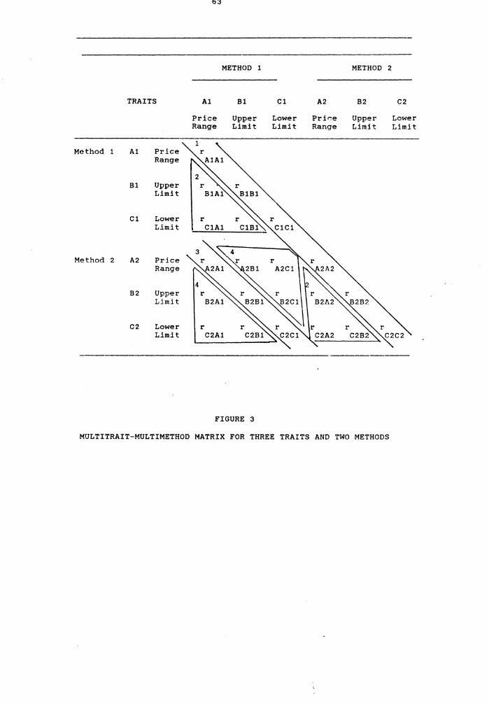
63

METHOD 1 METHOD 2

TRAITS Al Bl Cl A2 B2 C2

Price Upper Lower Price Upper Lower Range Limit Limit Range Limit Limit

Method 1 Al Price Range

Bl Upper Limit

Cl Lower r Limit ClAl

·Method 2 A2 Price Range

B2 Upper Limit

C2 Lower r Limit C2Al

FIGURE 3

MULTITRAIT-MULTIMETHOD MATRIX FOR THREE TRAITS AND TWO METHODS

64

TABLE 3

This table presents the retail prices that the personal computer is presently selling for in the Hamilton area. These retail prices represent six different brands of the computer described earlier.

RETAIL PRICES OF THE PERSONAL COMPUTER IN THE HAMILTON AREA

STORE 1 STORE 2 STORE 3 STORE 4 STORE 5 STORE 6

Brand

A $3300 $3500 $3300 $3400 ----- -----

B $4100 $4000 ----- $3900 $4000 -----

c $3100 $2900 $3000 $2900 $3000 $2900

D $3700 ----- ------ $3700 $3800 $3800

E $4000 $3900 $4000 $3900 $4000 -----

F $3300 $3500 ----- $3400 ----- $3400

65

DEPENDENT VARIABLES

There are three dependent variables in this study: (1)

absolute lower price limit, (2) absolute upper price limit, and

(3) acceptable price range. Individual price thresholds were

operationalized at the lowest and at highest price stimulus value

that produced a willingness to buy response. The individual price

thresholds were then used to establish the average group absolute

price thresholds. The absolute price range was operationalized

by measuring the difference between the individual absolute price

thresholds. That is, the difference between the upper and lower

price threshold for each of the subjects.

The dependent variables were measured via two different

methods: (1) the Stoetzel Method, and (2) the Own-category

method. A summary of these methods are presented below.

METHODS

Stoetzel Method

The Stoetzel (1954) method for measuring price thresholds

is simple and straightforward. Subjects were provided a detailed

description of a desktop personal computer, and a random list of

50 prices ranging from $1500 to $6400. The prices differed by a

constant interval of $100. The price thresholds were determined

by means of responses to two questions. The questions were:

(1) What is the minimum price that you would be willing to pay

for the personal computer (that is, below what price would

you seriously doubt the quality of the product?)

66

(2) What is the maximum Qrice that you would be willing to pay

for the personal computer (that is, beyond what price would

you feel it would not be worth paying more?)

The individual price responses to these two questions were

used to establish the individual lower and upper price

thresholds. More specifically, responses to the first question

set the subject's lower price limit, and responses to the second

question set the subject's upper price limit. The difference

between these responses set the individual acceptable price range.

Own-category Method

In this method, subjects were asked to judge the same set of

50 prices as in the Stoetzel method for the same personal

computer. Subjects were provided a description of the personal

computer and were presented with an envelope containing a set of

50 price slips that had been placed in the envelope in random

order. Each price slip contained only one price. The set of 50

prices contained prices from $1500 to $6400 and differed by a

constant interval of $100. Subjects were instructed to sort the

"price slips " into any number of piles they wished on the basis

of similiarity of the prices. After completing this task,

subjects were provided additional instructions. These

instructions required the subjects to place the piles of prices

they had created into three categories, representing those prices

they perceived as "acceptable," "unacceptable," or "neither

acceptable nor unacceptable." Subjects were allowed to

67

reconsider their initial evaluation. Then, subjects were provided

an envelope containing two sets of identification labels. These

labels were used to identify the price piles sorted earlier.

Subjects were to use the price labels to identify the price piles

as acceptable or unacceptable along a seven-point continuum

ranging from very acceptable to very unacceptable (Monroe 1971;

Petroshius 1983). After completing this price categorization, the

individual price thresholds were established by selecting the

lowest and highest price indicated by the subject as acceptable

to pay for the product. And the acceptable price range was

established by taking the difference between those scores.

Method Validation

Heeler and Ray (1972) have identified three basic approaches

to assessing validity: face, criterion, and construct validity.

The first approach, also known as consensus validity, is used

when an argument is made that the measurement is obvious and a

self-evident representation of the phenomenon being studied.

Criterion validity is more empirically based .in that it examines

if the scale correlates with other criteria in an expected

direction, or if it can differentiate the positions of "known

groups," or whether it can correctly predict some criterion

measure (Churchill 1979). Construct validity, the most

challenging and problematic of all the approaches, is also the

validation technique most directly related to the question of

what the scale is, in fact, measuring. To establish construct

validity of a measure (s), one must determine the measure(s)

68

convergent and discriminant validity.

Convergent validity is defined as the extent to which the

measure correlates with other measures designed to measure the

same thing. Discriminant validity is defined as the extent that a

measure behaves as expected (Churchill 1979). Discriminant

validity is determined by demonstrating that a measure does not

correlate very highly with another measure from which it should

differ (Peter 1981; Churchill 1979).

Evidence for convergent validity of a measure is presented

in the validity diagonal (3) of the MM matrix detailed in Figure

3 by the extent to which the correlations are significantly

different from zero and sufficiently large enough to encourage

further examination of construct validity. However, convergent

validity is only a necessary condition for construct validity.

Significantly high correlations could be due to method variance,

demand artifacts, or extraneous factors. As a result, evidence of

convergen~ validity is a necessary but not a sufficient criterion

for construct validity (Baggozi 1980). Therefore, discriminant

validity must be determined before construct validity can be

determined (Campbell and Fiske 1959). And discriminant validity

is determined by demonstrating that a measure does not correlate

very highly with another measure from which it should differ

(Peter 1981; Churchill 1979).

Figure 3, which was adapted from Campbell and Fiske (1959),

presents the MM matrix that was used in this dissertation. The

three traits {A, B, C) are each measured by two methods (1 and

2). Traits A, B, and C depict the lower price threshold, upper

69

price threshold, and acceptable price range, respectively, while

method 1 and 2 represent the Stoetzel method and Own-category

method, respectively.

The four essential elements of a multitrait-multimethod

matrix are identified by the numbers in the upper left hand

corner of each partitioned segment (Churchill 1979).

Diagonal 1 corresponds to the reliability of the alternative

methods of trait measurement through repeated measurement of the

same subjects.

The correlations between the same traits across methods is

known as the validity diagonal (3) which provides evidence of

convergent validity. The entries in the validity diagonal should

not only be statistically different from zero, but sufficiently

large enough for further examination of validity. Moreover, the

pattern of correlations should be compared to the heterotrait-

monomethod triangle (2) and the heterotrait-heteromethod triangle

( 4) •

Discriminant validity requires three comparisions. One,

correlations in the validity diagonal ( 3) should be higher than

the correlations that occupy the same row and column in the

heteromethod triangle (4). This means that the correlations

between two different measures of the same variable should be

higher than the correlations "between that variable and any other

variable which has neither trait nor method in common" (Campbell

and Fiske 1959, p.82). Two, the validity coefficients (diagonal

3) should be higher than the correlations in the hetertrait-

70

monomethod triangles (2) which means that the correlation within

a trait measured by different means must be higher than the

correlations between traits which have method in common. Three,

the patterns of correlations should be the same in all the

heterotrait triangles (both 2 and 4). ~he correlations within

each diagonal should be ranked from largest to smallest and the

same pattern of correlations should emerge. This is a check on

the significance of the traits when compared to the methods.

Table 4 outlines the formal summary of the above criteria

based upon .the pattern of correlations provided earlier in Figure

3.

PRODUCTS

The selection of the product used in this study was guided

by the following considerations and were adapted from Petroshius

(1983):

(1) The subjects should be potential purchasers and/or users of

the product.

(2) The product should normally be used by both males and

females to avoid sexual bias.

(3) The product selected should minimize subject prior price

knowledge.

Guided by these considerations, a personal computer was

selected. The personal computer was a product that was considered

as likely to be purchased by students of either sex. Further,

product price knowledge should be minimal since it is not a

frequently purchased product and enhances product price knowledge

71

TABLE 4

CRITERIA FOR CONVERGENT AND DISCRIMINANT VALIDITY IN THE CAMPBELL AND FISKE MULTITRAIT-MULTIMETHOD MATRIX

(THREE TRAITS AND TWO METHODS)

Convergent Validity

Correlations

( 1) r A2Al>O

r B2Bl>O

r C2Cl>O

The correlations should be statistically significant, greater then zero, and "sufficiently large."

Discriminant Validity

Correlation PatterB

(2) r r r r r A2A1> A2B1, A2C1, B2Al, C2A1

r r r r r B2Bl> A2Bl, C2Bl, B2Al, B2Cl

r r r r r C2Cl> A2Cl, B2Cl, C2Al, C2Bl

(3) r r r r r A2Al> BlAl, ClAl, B2A2, C2A2

r r r r r B2Bl> ClBl, BlAl, C2B2, B2A2

r r r r r C2Cl> ClAl, ClBl, C2A2, C2B2

(4) Within all heterotrait triangles, the pattern of intertrait correl-ations should be repeated across triangles. For example:

r r if BlAl> ClAl, the following should also result:

r r B2Al > C2Al

Criteria

Differences in correlations should be in the proper direction and statistically significant.

Differences in correlations should be in the proper direction and statistically significant.

Differences in correlations should be in the proper direction and statistically significant.

*Adapted from Bagozzi 1980, p.131

72

variability.

Subjects were provided with the following product

description:

The personal computer displayed at the front of the room is a desktop model having 640K internal memory. Features include dual 5.25 inch floppy disk drives that can store 360K each, 640x240 resolution color monitor with color card standard, parallel and serial ports, detached keyboard with clearly labeled and color-coded keypads, a calculator-style keypad, has 6 expan-sion slots, and comes with a MS-DOS operating system.

Sampling

The sample of subjects were selected from the Business

College student population at McMaster University. It has been

debated whether or not it is methodologically acceptable to use

students as subjects (Calder, Phillips, Tybout 1981, 1982, 1983;

Lynch 1982, 1983). Nevertheless, there are reasonable grounds for

using a college student population, particularly when college

students are buyers or potential buyers of a product(s). Since

the major purpose of this study is for theory/hypothesis and

method testing, and not directed at generalizing the results to

the general population, a college student convenience sample is

justified. Moreover, to increase realism in the experimental

setting, the product chosen for this study is reflective of the

type that college students would be likely to purchase.

(Interviews with sales managers at six retail computer outlets

confirmed the contention that students were active buyers of

personal computers) .

73

Sample Size

The Solomon 4-group design had a total of 4 groups to which

subjects were randomly assigned. In order to determine a

reasonable estimate of the reliability of the findings, and based

on practical conside~ations it was intended to have at least 40

subjects per group. In fact, data from 56 subjects from group 2

of the Solomon four-group design were used to establish

reliability and validity coefficients for the multimethod-

multitrait matrix.

Since the first two groups of the Solomon design required

subjects to attend two experimental sessions, there was a

possibility that subject mortality would occur during the

extended testing period. As a result, subjects were told that

that they would be rewarded for their participation by receiving

addition marks from their respective professors. This precaution

was used to minimize subject mortality over the two testing

periods. Despite the reward process, there was a larger than

expected mortality rate as outlined in Chapter IV.

A total of 420 subjects were randomly assigned to the four

groups. That is, each group was assigned 105 subjects. Of the

original 420 subjects, 351 subjects participated during the

course of the entire two-phase study. However, only data from 316

of the 351 subjects who participated during the second phase of

the study was used in the statistical analysis. It was the

posttest price threshold scores of Phase 2 that were used in the

factorial analysis.

Group counts in the factorials varied from a low of 56 to a

74

high of 105 which reflects the mortality rate, as well as method

measurement problems. As a result, the factorial analysis

resulted in an unequal or nonorthogonal design. Subsequently, the

two-way anovas were analyzed using three separate techniques

deemed to be most appropriate for the analysis of nonorthogonal

designs. These analysis techniques are detailed in Chapter IV.

Chapter IV provides details of the participation rates

during each phase of the study. It includes a summary of the

mortality rate, as well as unuseable results.

EXPERIMENTAL PROCEDURES

The research was conducted in two stages. The objectives of

the first stage was to pretest the two testing instruments. The

pretest was conducted over two phases reflecting the actual

experimental (the Solomon design) procedures outlined earlier.

The first phase established the subject's price limits and

acceptable price range where no market price inforamtion was

provided, and the second phase using the same subjects

established their price limits and acceptable price range when

market price information was presented.

The objectives of the second stage was to conduct the actual

experiment. It was conducted in two phases. Phase 1 objectives

were (1) to randomly assign subjects to each of the four groups

and to each of the two methods, and (2) to obtain the pretest

price threshold and acceptable price range scores for each

individual subject, as well as group scores for each of the two

75

methods. The objectives of phase 2 were (1) to introduce the

market.price information treatments, (2) to measure the price

thresholds and acceptable price range for each individual and for

each group as a result of those treatments, and (3) to obtain

reliability correlations from the pretest/posttest measurement of

Group 2, and (4) to establish validity coefficients using

individual price thresholds scores from the same group.

STAGE ONE/PRETEST OF THE INSTRUMENT

Prior to conducting the actual experiment, a pretest of the

testing instruments was conducted. A convenience sample of 34

subjects other than the subjects actually used in the experiment

were involved. The purpose of this pretest was to identify any

potential irregularities in the instruments before conducting the

actual experiment.

The same procedures were followed in the pretest as in the

actual experiment. Examination of the data and the procedures

revealed no identifiable problems. Consequently no procedural

changes were made in the testing instruments for use in the

actual experiment. A summary of the pretest results appear in

Table 5. Appendix E outlines the actual lower and upper price

limits, and acceptable price ranges in terms of absolute,

relative, and cumulative frequencies.

The results of phase l indicate the individual lower and

upper price limits, and acceptable price ranges for the subjects

when they received no price information. The mean lower price

limits were similar for both methods. The mean lower price limit

76

TABLE 5

INSTRUMENT PRETEST SUMMARY STATISTICS

PHASE l/NO PRICE INFORMATION TREATMENT

LOWER PRICE LIMIT

STOETZEL OWN-CATEGORY METHOD METHOD

UPPER PRICE LIMIT

PRICE RANGE

LOWER PRICE LIMIT

UPPER PRICE LIMIT

PRICE RANGE

---------------------- ----------------------N OF CASES 34 34 34 34 34 34 MINIMUM 15.000 20.000 5.000 15.000 20.000 5.000 MAXIMUM 38.000 60.000 32.000 41.000 59.000 33.000 MEAN 19.471 35.794 16.324 19.882 39.353 19.471 STANDARD DEV 6.161 9.224 7.466 6.362 10.015 7.033

PHASE 2/MARKET PRICE INFORMATION TREATMENT

LOWER PRICE LIMIT

STOETZEL OWN-CATEGORY METHOD METHOD

UPPER PRICE LIMIT

PRICE RANGE

LOWER PRICE LIMIT

UPPER PRICE LIMIT

PRICE RANGE

---------------------- ----------------------N OF CASES 34 MINIMUM 15.000 MAXIMUM 32.000 MEAN 22.941 STANDARD DEV 5.773

the the the

*MINIMUM 15.000 = MAXIMUM 38.000 = MEAN 19.471 = STANDARD DEV = the

34 34 34 34 27.000 4.000 15.000 29.000 45.000 29.000 35.000 55.000 37.794 14.353 20.794 39.794

4.635 6.252 5.688 6.660

lower price limit is $1500 upper price limit is $3800 mean price is $1947.10 standard deviation is $616.10

34 6.000

29.000. 19.000

5.705

77

for the Own-category method was slightly greater (x= 19.88, s.d.=

6.362) than the lower price limit for the Stoetzel Method

(x=19.47, s.d.= 6.161). The range of the lower price limits were

also similiar for the two methods except that the range was wider

for the Own-category method than the Stoetzel method. The lower

price limit for the Stoetzel method ranged from a low of $1500 to

high of $3800; the lower price limit for the Own-category method

ranged from a low of $1500 to a high of $4100.

There was more variability in subject upper price

limit than in the lower price limit for both methods. The mean

upper price limit for the Stoetzel method was smaller (x=35.794,

s.d.= 9.224) than for the Own-category method (x=39.353, s.d.=

10.015). However, the range of the upper price limits were quite

similar between the two methods. The range of the upper price

limit ranged from $2000 to $6000 for the Stoetzel method, and

ranged from $2000 to $5900 for the Own-category method.

The mean acceptable price range was wider for the Own-

category method (x=19.471, s.d.=7.033) than for the Stoetzel

method (x=16.324, s.d.=7.466). The mean acceptable price range

for the Stoetzel method ranged from a low of $500 to a high of

$3200. The Own-category method produced acceptable price ranges

from a low of $500 to a high of $3300.

During phase 2 of the pretest, subjects established their

price limits and acceptable price range after receiving market

price information. The mean lower price limit was greater for the

Stoetzel method (x=22.941, s.d.=5. 773) than for the Own-category

78

method (x=20. 794, s.d.=5.688). With the Stoetzel method, subjects

lower price limits ranged from $1500 to $3200. For the Own-

category method the lower price limit ranged from $1500 to $3500.

Most importantly, there was less variability in the lower price

limit for both methods when subjects were exposed to market price

information.

The mean upper price limit was greater for the Own-category

method (x=39.794, s.d.=6.660) than for the Stoetzel method

(x=37.294, s.d.=4.635). The upper price limit ranged from $2700

to $4500 for the Stoetzel method, and ranged from $2900 to $5500

for the Own-category. Again, there was less variability in the

upper price limit scores in the the market price information

treatment then in the no price information treatment of phase 1.

The mean acceptable price range was wider for the Own-

category method (x=19.000, s.d.=5.705) than for the Stoetzel

method (x=l4.353, s.d.=6.252). The acceptable price range for the

Stoetzel method ranged from a low of $400 to a high of $2900. The

Own-category method produced acceptable price ranges from a low

of $600 to a high of $2900. Again, there was less variability in

the acceptable price range scores in the market price information

treatment than in the no information treatment·for both methods.

In sum, the results indicate that subjects adjusted their

lower and upper price limits, and acceptable price ranges with

the introduction of market price information. The lower and upper

price limit increased with the introduction of market price

information for both methods. Moreover, the acceptable price

range was narrower in the market price information treatment than

79

the acceptable price range established when subjects were

presented with no market price information.

THE EXPERIMENT/PHASE ONE

Prior to the actual experiment, 420 subjects attending third

and forth year commerce classes were randomly assigned to each of

the four groups. Each group was assigned 105 subjects.

In the first phase of the actual experiment (the pretest

phase of the Solomon design), only subjects assigned to Group 1

and Group 2 of the Solomon design participated.

§.!.2~!~~1 ~!:2£~gy_r~. Each subject was given a response

booklet that was numbered on the upper right-hand corner at the

start of the session. A numbered card corresponding to the number

of the booklet was also supplied. This numbered card was used as

one means for proper identification of the subjects' booklets

during the second phase. Moreover, subjects were told to write

their name and student identification number at the top left hand

corner of the front page of the response booklet. They were told

that this information was to be used to aid in notifying their

professor of their participation in the experiment so that the

subject would receive their participation marks. They were also

told that once this was done, the front page of their response

booklet would be destroyed such that the researcher could not

identify subject responses. They were told that the researcher

was not interested in individual responses but only group

responses.

80

Each response booklet consisted of (1) an instruction

sheet; (2) two pages containing a product description, a series

of 50 prices ranging from $1500 to $6400 appearing in random

order, and t~e Stoetzel questions concerning the lowest and

highest price• the subjects were willing to pay for the product;

and (3) two pages of questions assessing subject familiarity with

personal computer prices, and some demographic quest ions.

Appendix A provides the response booklet used during the Stoetzel

procedure of Phase 1.

After all subjects had been seated, the experimenter gave

each subject the response booklet, and advised the subjects not

to turn the page until instructed to do so. The instructions

found on page 1 were read aloud to the subjects. After asking if

there were any questions, subjects were told to turn to page 2,

read the product description, and assume that they were seriously

interested in buying that product. After asking subjects if there

were any questions, they were told that there was no time limit

in completing the task and to put down their pens or ?encils and

look straight ahead upon completion of the experiment. Subjects

were then told to begin ..

After all subjects had completed the task, they were told to

place all materials in the envelope and to seal that envelope.

They were then told to await further instructions.

Own-category Procedure .. After subjects had finishing sealing

their envelopes, they were given another envelope containing the

Own-category method material, and told not to open it until

81

instructed to do so. The envelope contained instructions, a

response booklet, an envelope containing a set of 50 price slips,

an envelope containing two sets of price labels, and a few

questions assessing subject product and price knowledge. Appendix

B contains the contents of the response booklet used during the

Own-category procedure of Phase 1.

Subjects were told to empty the contents of the envelope on

their desks, and to write their name and student ID number where

indicated on the front page of the response booklet. The

instructions on the first page of the response booklet were read

to the subjects by the experimenter. After asking if therewere

any questions, subjects were told to turn to page 2, read the

product description, and assume that they were seriously

interested in buying that product. After reading the product

description, subjects were told to open the envelope marked

"Price Slips". Subjects were instructed to begin by sorting the

"price slips" into any number of piles they choose on the basis

of which prices seemed to belong together. The prices on the 50

price slips were identical to those prices provided in the

Stoetzel procedure.

When the subjects had completed this sorting task, they were

told to turn to page 3 for additional instructions. Those

instructions were read aloud by the experimenter, and required

the subjects to place the price piles they had created in one of

three positions on their desk. The price piles that represented

prices that were "acceptable" were to be placed on the left side

82

of the desk; price piles that were considered "unacceptable" were

placed on the right side, and price piles that were "neither

acceptable nor unacceptable" were placed in the center. The

subjects were told not to combine the separate price piles.

When subjects had completed this task, they were told to

turn to page 4 of the response booklet and read those

instructions along with the experimenter. At that time, subjects

were told to open the second envelope marked "Price Labels".

Inside that envelope were some paper clips, and two sets of seven

"label cards" for identifying the piles into price categories.

The price labels provided were:

Very Acceptable

Moderately Acceptable

Slightly Acceptable

Neither Acceptable nor Unacceptable

Slightly Unacceptable

Moderately Unacceptable

Very Unacceptable

The instructions required the subjects to label the pile or

piles of price slips on their desks using as many or as few of

the price labels as desired. Subjects were told if they ran out

of label cards to raise their hand and additional label cards

would be provided. When all the piles had been labeled, subjects

were told to secure the labeled piles with a paper clip and place

the secured piles inside the envelope marked "Price Labels".

After completing that task, subjects were asked to answer the

83

questions found on the last page of the response booklet. It

contained questions concerning recent purchase behavior and were

identical to the questions presented in the Stoetzel procedure.

When this task was completed, subjects were told to place all

materials back in the envelope and to seal it.

When all subjects had completed the entire procedure, they

were thanked for their participation, and were told that they

had completed the first phase of the study. The second phase of

the study would be conducted five days later. The subjects were

also reminded to bring the numbered card during the second

session.

RESULTS OF THE EXPERIMENT/PHASE 1

Subjects in Group 1 and Group 2 of the Solomon design

participated in the pretest phase of the experiment. Of the 105

subjects assigned to each of the two groups, 94 subjects in Group

1 and 78 subjects in Group 2 participated.

Table 6 presents the summary statistics for the price

threshold scores for each of the two methods. Appendix F details

the lower and upper price limits, and acceptable price ranges in

terms of absolute frequency, relative frequency, and cumulative

frequency for each of the subjects in groups 1 and 2.

There were no identifiable problems encountered during this

pretest phase of the study. Subsequently, there were no changes

made to the instruments for Phase 2 of the experiment.

There was little difference in the mean lower price limits

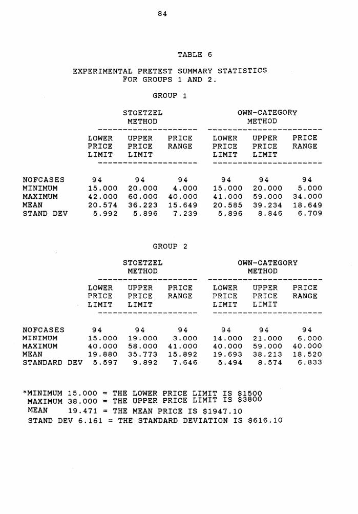
84

TABLE 6

EXPERIMENTAL PRETEST SUMMARY STATISTICS FOR GROUPS 1 AND 2.

GROUP 1

STOETZEL OWN-CATEGORY METHOD METHOD

LOWER UPPER PRICE LOWER UPPER PRICE PRICE PRICE RANGE PRICE PRICE RANGE LIMIT LIMIT LIMIT LIMIT

-------------------- ----------------------NOFCASES MINIMUM MAXIMUM MEAN STAND DEV

94 15.000 42.000 20.574 5.992

94 94 20.000 4.000 60.000 40.000 36.223 15.649

5.896 7.239

GROUP 2

94 94 94 15.000 20.000 5.000 41.000 59.000 34.000 20.585 39.234 18.649 5.896 8.846 6.709

STOETZEL OWN-CATEGORY METHOD METHOD

LOWER UPPER PRICE LOWER UPPER PRICE PRICE PRICE RANGE PRICE PRICE RANGE LIMIT LIMIT LIMIT LIMIT

-------------------- ----------------------NOFCASES 94 94 94 94 94 MINIMUM 15.000 19.000 3.000 14.000 21.000 MAXIMUM 40.000 58.000 41.000 40.000 59.000 MEAN 19.880 35.773 15.892 19.693 38.213 STANDARD DEV 5.597 9.892 7.646 5.494 8.574

*MINIMUM 15.000 = THE LOWER PRICE LIMIT IS $1500 MAXIMUM 38.000 = THE UPPER PRICE LIMIT IS $3800 MEAN 19.471 =THE MEAN PRICE IS $1947.10 STAND DEV 6.161 =THE STANDARD DEVIATION IS $616.10

94 6.000

40.000 18.520

6.833

85

and the variability in the lower price limit scores in group 1.

The mean lower price limit was only slightly greater for the Own-

category method (x=20.585, s.d.=5.896) than for the Stoetzel

method (x=20.574, s.d.=5.992). However, there was slightly over a

$300 difference in the upper price limit between the two methods,

and the variability was much greater in the.upper price limit

scores than in the lower price limit scores. The Own-category

method produced a higher mean upper price limit (x=39.234,

s.d.=7.239) than the Stoetzel method (x=36.223, s.d.=8.846).

Moreover, the acceptable price range was narrower for the

Stoetzel method (x=15.645, s.d.=7. 239) than for the Own-category

method (x=18.649, s.d.=6.709).

The summary data for Group 2 was similiar to that of Group

1. The lower price limit was slightly less for both methods than

in Group 1 with the Stoetzel method producing mean lower price

limits (x=19.880,s.d.=5.597) only slightly greater than the Own-

category method (x=19.693, s.d.=5.494). The mean upper price

limit was also slightly less than that reported by Group 1.

However, the mean upper price limit was once again larger for the

Own-category method (x=38.213, s.d.=8.574) than for the Stoetzel

method (x=35.773, s.d.=9.892). Again, there was greater

variability in the upper price limit scores than in the lower

price limit scores. The mean acceptable price range was also

similiar to the Group 1 results. The Own-category method mean

acceptable price range was greater (x=18.520, s.d.=6.833) than

that of the Stoetzel method (x=15.893, s.d.=7.640).

86

THE EXPERIMENT/PHASE TWO

In Phase 2 of the experiment, all four groups participated.

Groups 1 and Group 3 completed the Stoetzel and Own-category

procedures containing the experimental market price information

treatment, and Groups 2 and 4 completed both procedures without

receiving market price information.

Essentially, the same procedures were used in the second

phase of the study, with one exception. Group 2 and Group 4

received the same response booklets and instructions as in Phase

one. Group 1 and Group 3 received the same instructions and

response booklet as in phase one but with the addition of the

market price information treatment.

~!2~!~~1 ~EQ£~g~E~· In the second phase of the Stoetzel

procedure, two different instruction and response booklets were

presented to the subjects. Subjects in the low market price

knowledge treatment (Group 2 and Group 4) received the same

instructions and response booklets as those subjects during Phase

1. The subjects in the high market price knowledge treatment

received the same instructions and response booklets as in phase

one with the exception that market price information and the

manipulation check was introduced. Appendix C provides the

response booklet used in phase two of the experiment and includes

the market price information treatment.

Own-category Procedure. Two different response booklets were

distributed to the respondents. Subjects in the low market price

87

knowledge treatment were given the same instructions and response

booklets as in phase one. Subjects in the high market price

treatment groups were given the response booklet that contained

additional instructions and the market price information. Prior

to the beginning of the sorting tasks as described in phase 1,

subjects were asked to answer a series of questions based on the

market price information table to perform a manipulation check.

This check was done to assure that subjects had attended to the

market price information.

The instructions and sorting procedure were identical to

those as outlined in Phase 1. However, subjects in Groups 1 and

3 began the sorting procedure after they were given the market

price information, and completed the manipulation check.

After all subjects had completed their task, the envelopes

were collected, and subjects were thanked for their

participation. The sessions concluded with an informal debriefing

session where subjects were told the purpose of the study.

Appendix D contains the response booklet used in the Own-category

procedure.for the market price treatment condition.

DATA ANALYSIS

Data from the Solomon 4-group design were analyzed through a

series of 2 by 2 factorial analysis of variance. With this

analysis one can study the main effects, treatment and non-

treatment, and pretested and not pretested groups using F tests

for each of the three dependent variables, and for each of the

two methods. Moreover, one can test the interaction effect of

88

these two factors. The analytical design is presented in Table

7.

Test-Retest Reliability. The Pearson correlation coefficient

was calculated usi~g the individual lower and upper price limits,

and acceptable price ranges from the repeated measurement of

Group 2 for each of the two methods. As a result, there were 6

test-retest reliability coefficients for each of the two methods.

The resultant 6 by 6 correlation matrix was based on the

following correlations

(1) Stoetzel Method reliability coefficients for the lower

price threshold, upper price threshold, and acceptable

price range, respectively.

(2) Own-category method reliability coefficients for the

lower price threshold, upper price threshold, and

acceptable price range, respectively.

Q2g~!~Y£! Ysllgl!Y Q2~111£l~g!~· The Pearson correlation

coefficients from Group 2 were also used to establish the

validity coeef icients for each of the cells in the multitrait-

mul timethod matrix for the three traits and the two methods as

presented in Figure 3. Each correlation coefficient was tested

for statistical significance using t-tests. Moreover, the

correlation coefficients were examined for their conformity to

the pattern of correlations necessary to assess convergent and

discriminant validity. The pattern of correlations to be assessed

were provided earlier in Table 4.

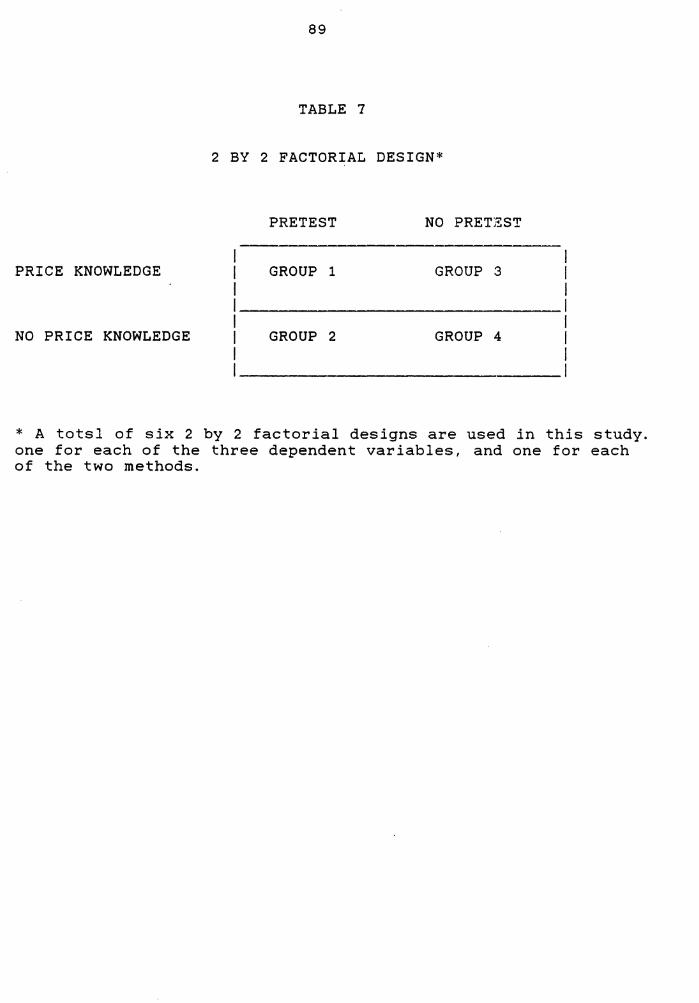
89

TABLE 7

2 BY 2 FACTORIAL DESIGN*

PRETEST

PRICE KNOWLEDGE GROUP 1 GROUP 3

NO PRICE KNOWLEDGE GROUP 2 GROUP 4

* A totsl of six 2 by 2 factorial designs are used in this study. one for each of the three dependent variables, and one for each of the two methods.

90

Hypothesis Testi!!.9.· The absolute lower price, absolute upper

price threshold, and the acceptable price range change scores

from Group 1 were tested using paired t-tests and two-way

analysis of variance on the posttest scores of groups 1 to 4.

CHAPTER SUMMARY

The research design and methodology for testing the

propositions presented in Chapter II were outlined. A Solomon 4-

Group design was argued as being an appropriate statistical

design to test the two propositions, and the multitrait-

mult~method design was used to test the Stoetzel and Own-category

methods for construct validity.

A summary of the instrument pretest results were presented

as well as the pretest scores of Phase 1 of the experiment.

CHAPTER IV

RESULTS AND ANALYSIS

This chapter presents the analysis and the results of the

experiment. First, all preliminary procedures performed on the

data are presented. Second, the statistical anaylsis of the

experimental data is discussed and includes: (1) the results of

the homogeneity of variance tests for each of the two-way

analysis of variance tests; and (2) the summaries of the two-way

analysis of variance that were performed on each of the dependent

variables for each of the two methods. Additional analyses are

also performed using paired t-tests for testing the empirical

hypotheses presented in Chapter III. The chapter concludes with

the examination of the construct validity of the two methods.

Preliminary Procedures

Preliminary procedures were conducted prior to the analysis

of the experimental data. These procedures included: (1)

examination of demand artifacts, (2) subject random assignment to

groups, (3) mortality rate, (4) unusable observations, and (5)

total subject participation.

Demand Artifacts

One debriefing question was examined to assess evidence of

demand artifacts. The question asked the subjects to indicate

their appraisal of the researcher's purpose of the experiment.

The responses to this question were examined to determine if. the

subjects guessed the true purpose of the experiment. The post hoc

91

92

analysis indicated that no subject quessed the true nature of the

research. Moreover, this finding held true for those subjects who

participated in both phases of the experiment.

Most of the subjects indicated that the purpose of the

experiment was to determine how knowledgeable subjects were about

personal computers or some aspect of price perception (e.g. how

much computers cost}. Others suggested that the University was

attempting to introduce student ownership of personal computers

into the Faculty of Commerce which is the case in the Faculty of

Engineering. Since none of the subjects quessed the true nature

of the experiment, no observations were deleted due to potential

demand artifacts.

Random Assignment to Groups

Subjects were matched with a master list developed by the

researcher. The master list identified each subject's randomized

assignment to the four groups. This was done to ensure that each

subject participated in his/her proper group session. Twenty-four

(24) subjects were found to participate in a group session to

which they were not randomly assigned. The experiment was

conducted in two locations and over two time periods. Those

subjects arrived at a location or time period which were more

convenient to them. In each of these cases, this situation

occurred where subjects were assigned to Group 1 or Group 2 which

required participation on two separate days. As a result, these

cases were deleted from the analysis. Moreover, one subject was

not assigned to any of the 4 groups but participated in both

93

phases. That subject, who was a friend of one of the partici-

pants,was also deleted from the analysis. These decisions were

made to maintain the random assignment to groups.

Mortality Rat:a

Group 1 and Group 2 lend themselves to the mortality rate

problem. Table 8 presents a summary of the number of subjects

remaining in each of the four treatment groups after subject

deletions based on the aforementioned causes. There would seem

to be a large number of non-participation during the two phases.

Sixteen (17.02%) of the subjects in Group 1 that participated in

first phase of the study did not participate in the second phase.

Likewise, nineteen (21%) subjects in Group 2 did not participate

during the second phase of the study. The experiment mortality

occured despite taking specific precautions. For example, all

participants were told both verbally and through two memos that

subjects assigned to groups 1 and 2 had to attend both

experimental sessions and at the location and time specified to·

earn their bonus marks.

Unusable Cases

Some of the price threshold scores had to be deleted for the

Own-category method. Eleven subjects (4.2%) either did not use

the label cards, or the price piles established were

inadvertently attached to other price labeled piles due to the

affixing of the price label with a paper clip. Where this

94

TABLE 8

EXPERIMENTAL TREATMENT GROUP SIZES AFTER DELETION OF UNUSABLE SUBJECT RESPONSES

PHASE 1 PHASE 2 MORTALITY POOR

ST oc ST oc ST oc ST OC

GROUPl 94 94 78 59 16 16 0 5

GROUP 2 75 75 56 56 19 19 0 0

GROUP 3 105 68 0 7

GROUP 4 77 70 0 0

TOTAL 169 169 316 253 35 35 0 12

ST = Stoetzel Method OC = Own-category Method Poor = Incomplete or Improper Price Assignment

NO

ST QC

0 14

0 0

0 30

0 7

0 51

No = Not Possible to Determine Lower and/or Upper Price Limit

95

occurred the observations were deleted. However, the price

thresholds established by those subjects using the Stoetzel

method were used in the subsequent statistical analysis. There

was no reason to believe that those ~rice threshold scores were

Lot accurate representations of subject price thresholds.

Total Subject Participation

Of the 420 subjects that were randomly assigned to the four

treatment groups, a total of 351 (not including the non-assigned

subject) subjects participated over both phases. After deleting

unusable responses a total of 316 (68.7%) subject responses were

used in the subsequent statistical analyses for the factorials.

A large number of subjects were not able to establish lower

or upper price thresholds using the Own-category method for price

threshold measurement. That is, while in ~.!..!. !!~~.Ql~ .£~~~~

subjects could indicate their price thresholds using the Stoetzel

method, it was not possible to establish the absolute price

thresholds using the Own-category method for fifty-one (16.2%) of

the subjects when the subjects used the Own-category method.

These subjects indicated low, medium, and high acceptable and

unacceptable prices. These scores were deleted from the analysis.

This would suggest that some buyers do not possess just one

acceptable price range but that they have multiple acceptable

price ranges at the lower, middle and higher price range of a

product. However, an alternative explanation of multiple price

ranges may be due to the fact that those subjects did not

understand the instructions provided for the Own-category method.

96

Nevertheless, this problem was not encountered during either the

pretesting of the entire instrument or during the pretesting of

subjects in Group 1 and Group 2 of Phase 1 of the experiment.

The fact that such a large proportion of subjects could not

set acceptable low and acceptable high prices using the Own-

category method for price threshold measurement constitutes a

systematic variance in the Own-category method that is not found

in the Stoetzel method. Most interesting, this finding was not

identified through prior research using the Own-category method.

As a result of these case deletions, non-participation, and

the measurement problem encountered for some subjects using the

Own-category method, the factorial designs were in all cases

unbalanced. Therefore, the subsequent two-way analysis of

variance tests were conducted using the most appropriate

statistical procedures for analyzing non-orthogonal designs. The

appropriate statistical procedures are (1) the classical

experimental approach, (2) the hierarchical approach, and (3) the

classical regression approach.

Measuring the Price Thresholds

!h~ ~12~!~~1 M~!h2Q· In this method the price threshold

scores were the prices that the subject indicated as being the

lowest and highest price that they would be willing to pay for

th~ personal computer. The difference between the individual

upper price threshold and lower price threshold set the

individual acceptable price range.

97

The Own-category Method. In this method, subjects rated the

various price piles they created containing the 50 price slips in

terms of a 7-point rating scale. The rating scale ranged from

very acceptable to very unacceptable. The scale center provided a

neutral neither acceptable nor unacceptable category. The

individual price threshold scores were established by selecting

the lowest and highest price of those prices that were contained

in the price piles labeled by the subjects as being slightly to

very acceptable. Again, the acceptable price range was

established by measuring the difference between the upper and

lower price threshold.

EXPERIMENTAL RESULTS

Descriptive Analysis

Prior to presenting the statistical analysis, the data are

presented descriptively. The description of the data is

presented separately for the acceptable price range, lower price

limit, and upper price limit. The means, standard deviations, and

sample sizes are presented in Tables 9 to 11.

~££~E!~Ql~ f~l£~ E~gg~. As detailed in Table 9, and using

Group 1 who received both treatments, there was a difference in

the mean acceptable price range due to the treatments when

subjects used the Stoetzel method. The mean acceptable price

range was narrower (x=13.667, s.d.=6.199) after subjects received

market price information than when market price information was

not presented (x=lS.649, s.d.=7.239). Moreover, there was less

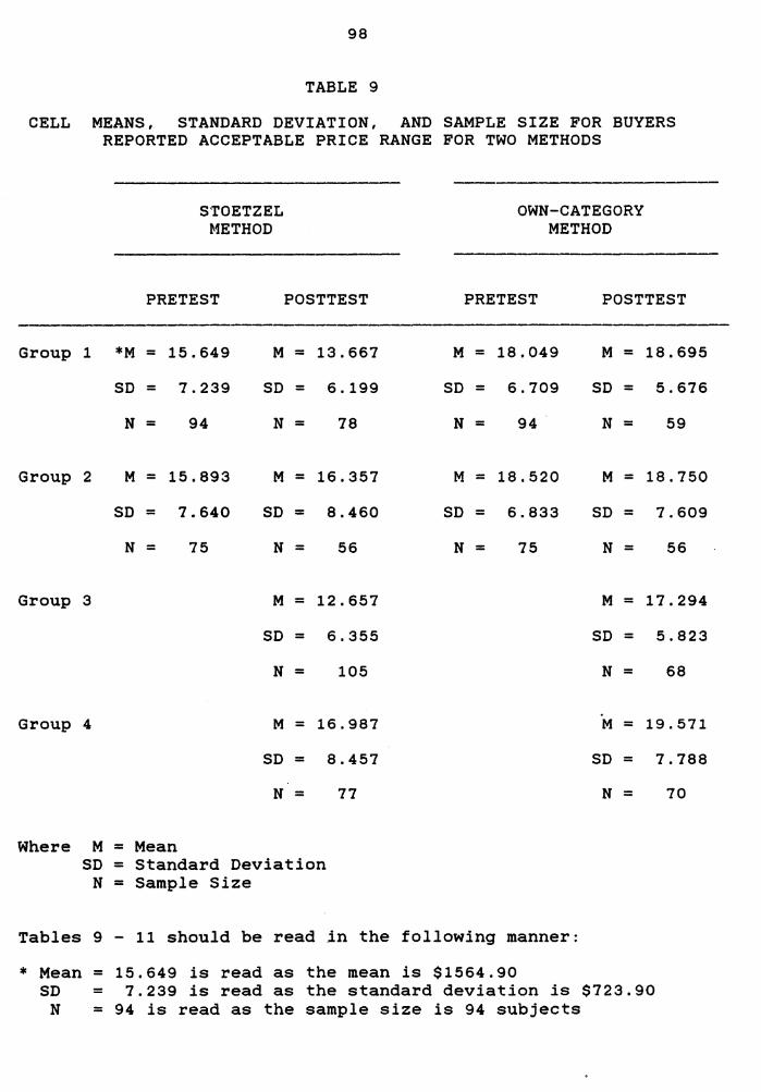
98

TABLE 9

CELL MEANS, STANDARD DEVIATION, AND SAMPLE SIZE FOR BUYERS REPORTED ACCEPTABLE PRICE RANGE FOR TWO METHODS

Group 1

Group 2

Group 3

Group 4

Where M SD

N

Tables 9

* Mean = SD =

N =

*M

SD

N

M

SD

N

= = =

-

STOETZEL METHOD

PRETEST

= 15.649 M

= 7.239 SD

= 94 N

= 15.893 M

= 7.640 SD

= 75 N

M

SD

N

M

SD

N

Mean

POSTTEST

= 13.667

= 6.199

= 78

= 16.357

= 8.460

= 56

= 12.657

= 6.355

= 105

= 16.987

= 8.457

= 77

Standard Deviation Sample Size

11 should be read .in the

15.649 is read as the mean

OWN-CATEGORY METHOD

PRETEST POSTTEST

M = 18.049 M = 18.695

SD = 6.709 SD = 5.676

N = 94 N = 59

M = 18.520 M = 18.750

SD = 6.833 SD = 7.609

N = 75 N = 56

M = 17.294

SD = 5.823

N = 68

M = 19.571

SD = 7.788

N = 70

following manner:

is $1564.90 7.239 is read as the standard deviation is $723.90

94 is read as the sample size is 94 subjects

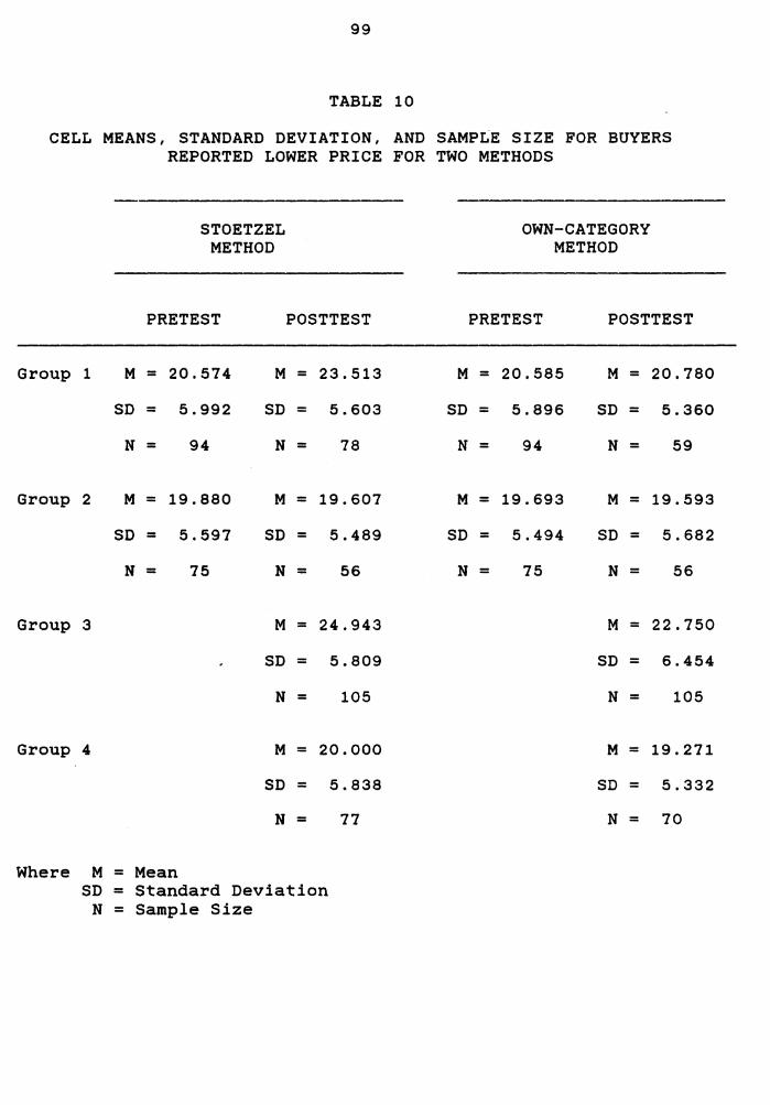
99

TABLE 10

CELL MEANS, STANDARD DEVIATION, AND SAMPLE SIZE FOR BUYERS REPORTED LOWER PRICE FOR TWO METHODS

Group 1 M

SD

N

Group 2 M

SD

N

Group 3

Group 4

Where M = SD =

N =

STOETZEL METHOD

PRETEST

= 20.574 M

= 5.992 SD

= 94 N

= 19.880 M

= 5.597 SD

= 75 N

M

SD

N

M

SD

N

Mean

POSTTEST

= 23.513

= 5.603

= 78

= 19.607

= 5.489

= 56

= 24.943

= 5.809

= 105

= 20.000

= 5.838

= 11

Standard Deviation Sample Size

M

SD

N

M

SD

N

OWN-CATEGORY METHOD

PRETEST POSTTEST

= 20.585 M = 20.780

= 5.896 SD = 5.360

= 94 N = 59

= 19.693 M = 19.593

= 5.494 SD = 5.682

= 75 N = 56

M = 22.750

SD = 6.454

N = 105

M = 19.271

SD = 5.332

N = 70

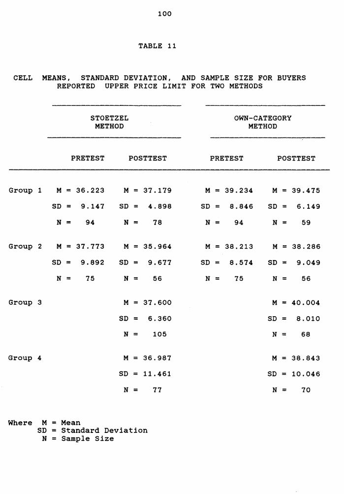
100

TABLE 11

CELL MEANS, STANDARD DEVIATION, AND SAMPLE SIZE FOR BUYERS REPORTED UPPER PRICE LIMIT FOR TWO METHODS

Group 1 M = SD =

N =

Group 2 M = SD =

N =

Group 3

Group 4

STOETZEL METHOD

PRETEST

36.223 M

9.147 SD

94 N

37.773 M

9.892 SD

75 N

M

SD

N

M

SD

N

POSTTEST

= 37.179

= 4.898

= 78

= 35.964

= 9.677

= 56

= 37.600

= 6.360

= 105

= 36.987

= 11.461

= 77

Where M = Mean SD = Standard Deviation

N = Sample Size

M

SD

N

M

SD

N

OWN-CATEGORY METHOD

PRETEST POSTTEST

= 39.234 M = 39.475

= 8.846 SD = 6.149

= 94 N = 59

= 38.213 M = 38.286

= 8.574 SD = 9.049

= 75 N = 56

M = 40.004

SD = 8.010

N = 68

M = 38.843

SD = 10.046

N = 70

101

variability in the acceptable price range scores in the market

price information treatment than in the no market price

treatment. This finding supports the hypothesis that subject

acceptable price range would narrow with the introduction of

market price information. However, when subjects useJ the Own-

category method, the mean acceptable price range moved in the

opposite direction as hypothesized. The mean acceptable price

range was slightly wider in the market price information

treatment (x=lS.695, s.d.=5.675) than in the no market price

information treatment (x=lS.049, s.d.=6. 709). There was, however,

less variability in the market price information condition.

In sum, support for the hypothesis that subject acceptable

price range would narrow with the introduction of market price

information was supported only with the results of the Stoetzel

method. However, the acceptable price ranges moved in the

opposite direction from that which was predicated using the Own-

category method. The acceptable price range was barely wider in

the market price information condition.

Change in the acceptable price range would have to be

accompanied by change in at least one of the price limits since

the lower and upper price limits establish individual acceptable

price range. As a result, the effect of market price information

on the lower and upper price limit was investigated.

Lo~~ Price Limits. Table 10 provides the summary statistics

for the lower price limit. The mean lower price limit increased

with the introduction of market price information for Group 1

102

using the Stoetzel method. The mean lower price limit in the no

market price information and market price information treatments

were x=20.574 (s.d.=5.992) and x= 23.513 (s.d.=5.603)

respectively. Again, there was less variability in the lower

price limit in the market price information treatment. However,

the mean lower price limit increase only slightly with the

exposure to market price information using the Own-category

method. The mean lower price limit in the no market price

information condition was x=20.585 (s.d.=5.896), and x=20.780

(s.d.=5.360) when subjects were provided market price

information. Again, less variability occured in the market price

information condition.

The mean lower price limits were similar for the two methods

when no m~rket price information was presented. However, the

impact of market price information was greater in the Stoetzel

method (x=23.513, s.d.=5.603) than in the Own-category method

(x=20.780, s.d.=5.360).

When using the post-test lower price limit scores for all

four groups, the introduction of market price information had a

greater impact on the lower price limit in the Stoetzel method

then in the Own-category method. Using the Stoetzel method, the

lower price limits were greater for the two groups that received

market price information than the two groups that received no

market price information. The mean lower price limits for Groups

1 and 3 which received market price information were x=23.513

(s.d.=5.603) and x=24.943 (s.d.=5.809). The mean lower price

limits for the no market price information Groups 2 and 4 were

103

x=19.607 (s.d.=5.489) and x=20.000 (s~d.=5.838). The variability

in the lower price limits was quite similar among the four

groups.

The mean lower price limits, also, increased with the

introduction of market price information using the Own-category

method. However, market price information had less of an impact

on the lower price limit than the Stoetzel method. The mean lower

price limit increased only slightly when market price information

was presented to the subjects in Group 1. In the no market price

information treatment, the mean lower price limit was x=20.585

(s.d.=5.896) versus a mean lower price limit of x=20.780

(s.d.=5.360) with the introduction of market price information.

Moreover, there was less variability in the lower price limits

when subjects set their lower price limits with market price

information available.

When comparing all four groups, the lower price limits were

greater for those groups that received market price information

than for those groups which received no such information. The two

groups receiving price information had mean lower price limits of

x=20.780 (s.d.=5.360) and x=22.750 (6.454) respectively. The mean

lower price limits were lower and more similar for the two groups

that received no price information. The mean lower price limits

were x=19.593 (s.d.=5.682) and x=19.271 (s.d.=5.332).

In sum, the mean lower price limits increased with the

introduction of market price information for both methods.

However, the introduction of market price information had a

104

greater impact on the lower price limits whe~ subjects used the

Stoetzel method than when they used the Own-category method.

Upper Price Li~it. Table 11 presents the summary statistics

for the upper price limits. The mean upper price limit increased

only slightly with the introduction of market price information

for subjects in Group 1. The mean upper price limit was x=36.223

(s.d.=9.147) in the no market price information treatment, and

x=37.179 (s.d.=4.894) when the same subjects established their

upper price limits with market price information using the

Stoetzel method. Moreover, the market price information treatment

reduced the variability in the upper price limit scores

dramatically.

The mean upper price limits also increased with the

introduction of market price information when the Own-category

method was used. However, the increase was marginal. The mean

upper price limit when no market price information was presented

was x=39.234 (s.d.=8.846), and with the introduction of market

price information was x=39.475 (s.d.=6.149). Again, variability

decreased in the market price information treatment.

When all four groups were considered, the mean upper price

limits were greater for the groups (1 and 3) receiving market

price information than the groups (2 and 4) receiving no price

information for both methods. For the Stoetzel method, the mean

lower price limits were x=37.179 (s.d.=4.898) and x=37.600

(s.d.=6.360) when market price information was provided, and

x=35.964 (s.d.=9.677) and x=36.987 (11.461) where market price

105

information was absent. For the Own-category method, the mean

upper price limits in the market price information treatment

groups were x=39.475 (s.d.=6.149) and x=40.004 (s.d.=8.010), and

x=38.286 (s.d.=9.049) and x=38.843 (s.d.=10.046) for the no

market price information tr~atment groups. Again, there was less

variability in the market price information treatment groups.

Moreover, there was greater variability in the upper price limit

scores using the Own-category method than when the Stoetzel

method.

In sum, the upper price limits increased with the

introduction of market price information in both methods.

Moreover, variability in the upper price limit scores decreased

when subjects were provided market price information than when no

market price information was not available.

STATISTICAL ANALYSIS

After deletion of unusable observations, 316 observations

were used in the subsequent analysis. The analysis included an

investigat~on into the homogeneity of variance assumption of the

groups in the experiment as well as the standard two-way analysis

of variance tests conducted on the original data.

While analysis of variance conducted on factorial designs

have been shown to be robust to violations of the homogeneity of

variance assumption, the ANOVA is not robust to outliers (Daniel

1960; Barnett and Lewis 1978). Therefore, exploratory data

analysis was conducted on the data and subsequently outliers were

identified and deleted. As a result, two-way analysis of variance

106

results are presented for both the full data, as well as for the

data with outliers deleted.

Homogeneity of Variance Assumption Results

Typically, researchers do not test for the homogeneity of

variance assumption since the hypothesis test is fairly robust to

the violation of this assumption when cell sizes are equal.

However, the violation of the homogeneity assumption can distort

conclusions on tests of significance when cell sizes are unequal

and therefore non-orthogonal {Cooley and Lohnes 1971; Kirk 1968;

Winer 1971; Speed et al. 1978). Moreover, while the F-test is

robust to certain violations of assumptions, factorials are by no

means robust against outliers {Daniel 1960; Barnett and Lewis

1978). As a result, the Bartlett-Box F univariate homogeneity of

variance test was conducted on the full data, as well as on the

data after deleting outliers.

Bartletts-Box F univariate homogeneity of variance tests

were conducted for each of the dependent variables within each of

the two measurement methods. The results of the Bartlett-Box F

hypothesis tests for the full data and data with outliers deleted

are reported in Table 12 and 13.

The results of the univariate tests of the homogeneity of

variance assumption based on the full data failed to reject (p >

0.05) the hypothesis of equal population variances when the

lower price threshold was tested for each of the two methods,

but produced strong statistical evidence (p < 0.05) to reject the

107

TABLE 12

RESULTS OF BARTLETT-BOX F AND COCHRAN C TEST

OF HOMOGENEITY OF VARIANCE

(FULL DATA)

THE STOETZEL METHOD

Univariate Homogeneity of Variance Tests

Lower Price Limit Bartlett-Box F {3,157328) = Upper Price Limit Bartlett-Box F {3,157328) = Price Range Bartlett-Box F (3,157328) =

Lower Price Limit Cochran C*(78,4) = 0.26345,

Upper Price Limit Cochran c (78,4) = 0.45383,

Price Range Cochran C (78,4) = 0.33256,

THE OWN-CATEGORY METHOD

Univariate Homogeneity of Variance Tests

Lower Price Limit Bartlett-Box F (3,109468) = Upper Price Limit Bartlett-Box F {3,109468) = Price Range Bartlett-Box F (3,109468) =

Lower Price Limit Cochran c (62,4) = 0.31772,

Upper Price Limit Cochran c (62,4) = 0.35439,

Price Range Cochran c (62,4) = 0.32843,

* The Cochran c is an approximate Test.

0.11880,

21.94341,

4.51882,

1.07279,

5.01241,

3.49967,

p = .949

p = .ooo p = .004

p = 1.000

p = 0.011

p = 1.000

p = .359

p = .002

p = .015

p = 1.000

p = 0. 9"79

p = 1.000

108

TABLE 13

RESULTS OF BARTLETT-BOX F AND COCHRAN C TEST

OF HOMOGENEITY OF VARIANCE

(WITH OUTLIERS DELETED)

THE STOETZEL METHOD

Univariate Homogeneity of Variance Tests

Lower Price Limit Bartlett-Box F (3,154819) = 2.28061,

Upper Price Limit Bartlett-Box F (3,142117) = 12.46387,

Price Range Bartlett-Box F (3,151813) = 2.50428,

Lower Price Limit Cochran c (78,4) = 0.28860,

Upper Price Limit Cochran C (62,4) = 0.35434,

Price Range Cochran C (62,4) = 0.32782,

THE OWN-CATEGORY METHOD ----

· Univariate Homogeneity of Variance Tests

Lower Price Limit Bartlett-Box F (3,107584) = .47967,

Upper Price Limit Bartlett-Box F (3,108716) = 5.44969,

Price Range Bartlett-Box F (3,108763) = 2.79519,

Lower Price Limit Cochran c (62,4) = 0.29255,

Upper Price Limit Cochran c (62,4) = 0.36444,

Price Range Cochran c (62,4) = 0.32515,

p = .077

p = .000

p = .058

p = 1.000

p = .979

p = .837

p = .696

p = .001

p = .039

p = 1.000

p = .777

p = 1.000

109

hypothesis of equal group variances for the upper price threshold

and the price ranges for each of the methods. Moreover, when the

homogeneity of variance tests were conducted on the data with

out 1 iers deleted, results remained the same with the except ion

that the homogeneity of variance assumption was not rejected for

the Stoetzel price range.

Despite the rejection of the homogeneity of variance

assumption in most cases, the magnitude of the degrees of freedom

associated with these hypotheses tests are such that even a

slight variation in the dispersion matrix would result in a

rejection of the hypothesis. In this situation, the degrees of

freedom exceeded 107,583 in each case. Referring to the highly

conservative nature of the Bartlett-Box F test, some authors

suggest that the Bartlett-Box F test is so powerful that it is

rare that the homogeneity of variance test would not be rejected

when research is conducted on large samples (Cooley and Lohnes

1971; Winer 1971).

In lieu of the highly sensitive nature of the Bartlett-Box

F test, the homogeneity of variance assumptions were retested

utilizing Cochran's Procedure. Cochran's homogeneity of variance

test is not as sensitive as the Bartlett-Box F test, but is often

used as a homogeneity of variance test procedure (Winer 1971).

However, it should be noted that the Cochran test is an

approximate test (Winer 1971).

As reported in Table 12 and 13, the results of Cochran's

univariate tests of the homogeneity of variance assumption based

110

on the full data failed to reject the hypothesis of equal

population variances for each dependent variable except the

Stoetzel upper price limit. The upper price limit was found to be

significant at p = 0.011. Moreover, testing on the data after

outliers were deleted failed to reject the hypothesis of equal

variance assumption for all the dependent variables.

As a result of the highly conservative nature of the

Bartlett Box-F test, and the failure to reject the homogeneity of

variance assumptions based on Cochran's procedure, except in the

case of the Stoezel upper price limit for the full data,

subsequent statistical analyses were conducted on the data.

Two-way Anovas and Hon-Orthogonal Designs

A major complication arises in the analysis of a factorial

design when the cell frequencies are not equal. With equal cell

frequencies or orthogonal designs, the independent variables are

totally independent or uncorrelated and the statistical analysis

is straightforward. However, as cell frequencies become unequal,

the independent variables become dependent and correlated or

nonorthogonal. Therefore, if the number of cases falling in each

cell are unequal, the calculation of various components of the

ANOVA as well as the interpretation of the results becomes more

involved since the independent variables are confounded with one

another and the classical ANOVA might not yield correct

conclusions {Spector 1980; Overall and Spiegel 1969}. For

example, the saturated model component sum of squares will not

add to the total main effects sum of squares because the main

111

effects will not usually.be independent of each other and the

interaction effects will not be independent of the main effects.

Moreover, in some cases the total additive model will be

significant while neither of the main effects will be

significant.

Overall and Spiegel (1969), and Spector (1980} recommend the

use of three approaches for handling nonorthogonal analysis of

variance: ( 1) classical experimental design approach, ( 2)

hierarchical approach (weighted least squares), and (3) classical

regression approach. A short summary of these techniques are

presented below.

Classical Experimental Design. In this approach, all three

components of the sum of squares (SS) are made orthogonal to one

another by imposing a certain hierarchy. The interaction

component is defined as the difference between the sum of squares

explained by the total joint effect of the main effects and the

additive effects of the main effects. In other words, the

interaction component is given by the residual components of the

effects of the mairi effects. The error component is likewise

defined by the residual sum of squares. Because the main effects

are not orthogonal, the sum of squares for each of th~ main

effects will not add to the sum of squares for the saturated

model. Therefore, the classical experimental design approach

assigns only that portion of the additive effects of the main

effects that is not accounted for by each of the main effects

adjusted for the other.

The most important difference of this design from the

112

orthogonal design is that if the main effects are strongly

associated, it is possible to have a result in which the additive

effect as a whole is significant while neither of the individual

main effects are significant. This occurs because each factor

receives credit only for the incremental sum of squares that it

adds to the effects of the other factor. As a result, the

individual main effects do not add to the saturated model sum of

squares, and incorrect inferences can be made.

lii~~~~£hi£~l ~22~2~£h· This approach is also called

'stepdown analysis' (Overall and Spiegel 1969). In this

procedure the sum of squares of the main effects are decomposed

hierarchically. The effects are not tested during the

decomposition process. Rather, testing occurs after the final

mean square error is obtained. The mean square error reflects the

variation remaining after all effects have been removed.

Unlike the classical approach where the sum of squares are

decomposed hierarchically between types of effects, in the

hierarchical approach sum of squares are decomposed

hierarchically between types of effects and also within the

factor main effects. The procedure for significance testing is

the same as in the classical approach. The only difference is

that if the additive effect is significant, at least one of the

main effects will always be significant.

Ql~~~i£~l R~g~~~~i2n ~22~2~£h· This approach partitions

individual effects by adjusting for all the other effects. The

main characteristic of this approach is the examination of a

113

given effect only after the effects of all the others, including

the interaction, are adjusted for.

In sum, all three approaches will produce exactly the same

result if every cell of the ANOVA has exactly the same number of

cases. But, the three approaches will differ for most

nonorthogonal designs. However, for a two-way analysis of

variance, the three approaches will differ only in handling the

main effects. The stronger the association (positive) between the

two main effects, the greater will be the discrepancy between the

joint additive (saturated model) effect and the sum of the main

effects. If the association is strong and positive, it is

possible that none of the main effects are significant although

the joint effect is. Therefore, it is important to examine the

additive effect in addition to the effects of each factor

(Overall and Spiegel 1969; Spector 1980).

Two-Way Analysis of Variance Results

Since this study makes use of unbalanced designs and can

produce different results depending on the analysis approach

used, al 1 three approaches were used and compared before a

conclusion was made. Summaries of the two-way analysis of

variance results appear in Tables 14 to 25. Each table provides

selected statistics for each of the two-way analysis of variance

approaches mentioned earlier. Moreover, the analysis was

conducted using the full data as well as after deleting the

outliers.

For the two-way analysis of variance tests, the three

114

TABLE 14

SUMMARY OF THE TWO-WAY ANALYSIS OF VARIANCE TESTS

SOURCE

MAIN EFFECT

TREATMENT

TEST

INTERACTION

TOTAL

1

USING THREE APPROACHES

FOR THE STOETZEL LOWER PRICE LIMIT

(FULL DATA)

CLASSICAL EXPERIMENTAL

METHOD

1 2 F p

25.071 .. ooo

47.910 .001

2.340 .127

0.620 .432

REGRESSION METHOD

F p

23.273 .000

45 .141 .ooo

1. 916 .167

0.620 .432

F-value corresponds to the F statistic

2

HIERARHCICAL METHOD

F P

25.071 .ooo

47.801 .000

2.340 .127

0.620 .432

P corresponds to the probability value of the F-statistic·

DF

2

1

1

1

316

TABLE 15

SUMMARY OF THE TWO-WAY ANALYSIS OF VARIANCE TESTS

SOURCE

MAIN EFFECT

TREATMENT

TEST

INTERACTION

TOTAL

1

USING THREE APPROACHES

FOR THE STOETZEL LOWER PRICE LIMIT

(OUTLIERS DELETED)

CLASSICAL EXPERIMENTAL

METHOD

1 F p

37.197 .000

72.172 .000

2.136 .145

1.514 .220

2

REGRESSION METHOD

F p

34.574 .000

68.129 .000

1.429 .233

1.514 .220

F-value corresponds to the F statistic

2

HIERARCHICAL METHOD

F p

37.197 .000

72.259 .ooo 2.136 .145

1.514 .220

P corresponds to the probability value of the F-statistic

OF

2

1

1

1

302

llb

TABLE 16

SUMMARY OF THE TWO-WAY ANALYSIS OF VARIANCE TESTS

USING THREE APPROACHES

FOR THE STOETZEL UPPER PRICE LIMIT

(FULL DATA)

CLASSICAL REGRESSION HIERARCHICAL EXPERIMENTAL METHOD METHOD

METHOD

1 2 SOURCE F p. F p F p DF

MAIN EFFECT 0.681 .507 0.730 .483 0.681 .507 2

TREATMENT 0.854 .356 0.925 .337 0.857 .358 1

TEST 0.515 .473 0.577 .448 0.515 .473 1

INTERACTION 0.100 .752 0 .100 .752 0.100 .752 1

TOTAL 316

1 F-value corresponds to the F statistic

2 P corresponds to the probability value of the F-statistic

117

TABLE 17

SUMMARY OF THE TWO-WAY ANALYSIS OF VARIANCE TESTS

SOURCE

MAIN EFFECT

TREATMENT

TEST

INTERACTION

TOTAL

1

USING THREE APPROACHES

FOR THE STOETZEL UPPER PRICE LIMIT

(OUTLIERS DELETED)

CLASSICAL EXPERIMENTAL

METHOD

1 2 F p

4.917 .008

9.469 .002

0.352 .553

0.020 .889

REGRESSION METHOD

F p

4. 711 .010

9.185 .003

0.308 .579

0.020 .889

F-value corresponds to the F statistic

2

HIERARCHICAL METHOD

F p

4.917 .008

9.482 .002

0.352 .553

0.020 .889

P corresponds to the probability value of the F-statistic

DF

2

1

1

1

302

118

TABLE 18

SUMMARY OF THE TWO-WAY ANALYSIS OF VARIANCE TESTS

USING THREE APPROACHES

FOR THE STOETZEL ACCEPTABLE PRICE RANGE

(FULL DATA)

CLASSICAL EXPERIMENTAL

METHOD

1 2 '

REGRESSION METHOD

HIERARCHICAL METHOD

SOURCE F p F p F p

MAIN EFFECT 9.676 .000 8.750 .000 9.676 .000

TREATMENT 19.219 .000 17.489 .ooo 19.201 .000

TEST 0 .150 .699 0.051 .821 0.150 .699

INTERACTION 0.954 .330 0.954 .330 0.954 .330

TOTAL

1 F-value corresponds to the F statistic

2 P corresponds to the probability value.of the F-statistic

DF

2

1

1

1

316

119

TABLE 19

SUMMARY OF THE TWO-WAY ANALYSIS OF VARIANCE TESTS

USING THREE APPROACHES

FOR THE STOETZEL ACCEPTABLE PRICE RANGE

(OUTLIERS DELETED)

CLASSICAL REGRESSION HIERARCHICAL EXPERIMENTAL METHOD METHOD

METHOD

1 2 SOURCE F p F p F p OF

MAIN EFFECT 7.692 .001 6.710 .001 7.692 .001 2

TREATMENT 15.370 .000 13.376 .000 15.355 .000 1

TEST 0.028 .867 0.004 .948 0.028 .867 1

INTERACTION 1.823 .187 1.823 .178 1.823 .187 1

TOTAL 302

1 F-value cprresponds to the F statistic

2 P corresponds to the probability value of the F-statistic

120

TABLE 20

SUMMARY OF THE TWO-WAY ANALYSIS OF VARIANCE TESTS

USING THREE APPROACHES

FOR THE OWN-CATEGORY LOWER PRICE LIMIT

(FULL DATA)

CLASSICAL REGRESSION HIERARCHICAL EXPERIMENTAL METHOD METHOD

METHOD

1 2 SOURCE F p' F p F p DF

MAIN EFFECT 6.455 .002 5.927 .003 6.455 .002 2

TREATMENT 11.655 .001 10.622 .001 11. 496 .001 1

TEST 1.414 .235 1.386 .. 240 1.414 .235 1

INTERACTION 2.378 .124 2.371 .124 2.378 .124 1

TOTAL 252

1 F-value corresponds to the F statistic

2 P corresponds to the probability value of the F-statistic

121

TABLE 21

SUMMARY OF THE TWO-WAY ANALYSIS OF VARIANCE TESTS

USING THREE APPROACHES

FOR THE OWN-CATEGORY LOWER PRICE LIMIT

(OUTLIERS DELETED)

CLASSICAL REGRESSION HIERARCHICAL EXPERIMENTAL METHOD METHOD

METHOD

1 2 SOURCE F p F p F p DF

MAIN EFFECT 6.531 .002 6.183 .002 6.531 .002 2

TREATMENT 11.970 .001 11. 282 .001 11. 727 .001 1

TEST 1.336 .249 1.323 .251 1.336 .249 1

INTERACTION 0.984 .322 0.984 .322 0.984 .322 1

TOTAL 249

1 F-value corresponds to the F statistic .

2 P corresponds to the probability value of the F-statistic

122

TABLE 22

SUMMARY OF THE TWO-WAY ANALYSIS OF VARIANCE TESTS

USING THREE APPROACHES

FOR THE OWN-CATEGORY UPPER PRICE LIMIT

(FULL DATA)

CLASSICAL REGRESSION HIERARCHICAL EXPERIMENTAI METHOD METHOD

METHOD

1 2 SOURCE F p F p F p DF

MAIN EFFECT 0.753 .472 0.747 .475 0.753 .472 2

TREATMENT 1. 253 .264 1.242 .266 1. 230 .268 1

TEST 0.276 .600 0.276 .600 0.276 .600 1

INTERACTION 0.000 .995 o.ooo .995 0.000 .995 1

TOTAL 252

1 F-value corresponds to the F statistic

2 P corresponds to the probability value of the F-statistic

TABLE 23

SUMMARY OF THE TWO-WAY ANALYSIS OF VARIANCE TF.STS

USING THREE APPROACHES

FOR THE OWN-CATEGORY UPPER PRICE LIMIT

(OUTLIERS DELETED)

CLASSICAL EXPERIMENTAL

METHOD

1 2

REGRESSION METHOD

HIERARCHICAL METHOD

SOURCE F p F p F p

MAIN EFFECT 0.460 .632 2.487 .617 0.460 .632

TREATMENT 0.825 .365 0.879 .349 0.806 .370

TEST 0.114 .736 0.115 .735 0.114 .736

INTERACTION 0.139 .710 0.139 . 710 0 .139 .710

TOTAL

1 F-value corresponds to the F statistic

2 P corresponds to the probability value of the F-statistic

DF

2

1

1

1

249

124

TABLE 24

SUMMARY OF THE TWO-WAY ANALYSIS OF VARIANCE TESTS

USING THREE APPROACHES

FOR THE OWN-CATEGORY ACCEPTABLE PRICE RANGE

(FULL DATA)

CLASSICAL EXPERIMENTAL

METHOD

REGRESSION METHOD

HIERARCHICAL METHOD

1 2 SOURCE F p F p F p

MAIN EFFECT 1.149 .319 0.970 .380 1.149 .319

TREATMENT 2.197 .140 1.845 .176 2.177 .141

TEST 0.121 .729 0.114 .736 0.121 .729

INTERACTION 1.674 .197 1.674 .197 1.674 .197

TOTAL

1 F-value corresponds to the F statistic

2 P corresponds to the probability value of the F-statistic

DF

2

1

1

1

252

TABLE 25

SUMMARY OF THE TWO-WAY ANALYSIS OF VARIANCE TESTS

USING THREE APPROACHES

FOR THE OWN-CATEGORY ACCEPTABLE PRICE RANGE

(OUTLIERS DELETED)

CLASSICAL EXPERIMENTAL

METHOD

1 2

REGRESSION METHOD

HIERARCHICAL METHOD

SOURCE F p F p F p

MAIN EFFECT 0.707 .494 0.555 .575 0.707 .494

TREATMENT 1.294 .256 1.008 .316 1. 273 . 260

TEST 0.140 .709 0.120 .730 0.140 .709

INTERACTION 1.755 .187 1.755 .187 1. 755 . 187

TOTAL

1 F-value corresponds to the F statistic

2 P corresponds to the probability value of the F-statistic

DF

2

1

1

1

249

126

approaches differed only in the handling of the main effects.

More specifically, in all cases, one would arrive at the same

conclusion with respect to the significance or non-significance

of the two main effects no matter what approach was used with one

basic exception. In comparing the ANOVA results between the full

data and the data with outliers deleted,

threshold scores for the Stoetzel method

the upper price

were found to be

significantly different only when outliers were deleted. This

difference is probably due to the fact that the deletion of the

outliers reduced the within group variability for the two groups.

Full Data Results. The analysis of the ANOVAS using the full

data indicated that the lower price threshold for both methods,

the joint additive effect of treatment and testing was

significant, as was the main treatment effect, while the main

testing effect and the interaction effect were both

nonsignif icant. The upper price threshold for the Own-category

acceptable price range, the joint additive effect of treatment

and testing, the main treatment and testing effect, and the

interaction effect were all found to be nonsignificant. The

acceptable price range for the Own-category method, main

treatment and testing effects, as well as the interaction effect

were nonsignif icant. However, there was a significant main

treatment effect on the Stoetzel acceptable price range, while

the main testing effect and interaction effect were found to be

non-significant.

In both the Stoetzel and Own-category method, the mean

lower price threshold scores of the treatment groups were

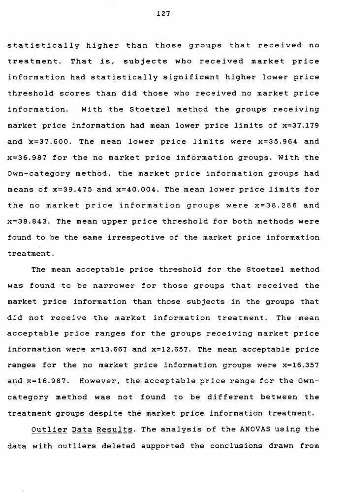
127

statistically higher than those groups that received no

treatment. That is, subjects who received market price

information had statistically significant higher lower price

threshold scores than did those who rec~ived no market price

information. With the Stoetzel method the groups receiving

market price information had mean lower price limits of x=37.179

and x=37.600. The mean lower price limits were x=35.964 and

x=36.987 for the no market price information groups. With the

Own-category method, the market price information groups had

means of x=39.475 and x=40.004. The mean lower price limits for

the no market price information groups were x=38.286 and

x=38.843. The mean upper price threshold for both methods were

found to be the same irrespective of the market price information

treatment.

The mean acceptable price threshold for the Stoetzel method

was found to be narrower for those groups that received the

market price information than those subjects in the groups that

did not receive the market information treatment. The mean

acceptable price ranges for the groups receiving market price

information were x=13.667 and x=12.657. The mean acceptable price

ranges for the no market price information groups were x=16.357

and x=16.987. However, the acceptable price range for the Own-

category method was not found to be different between the

treatment groups despite the market price information treatment.

Q~!!!~~ Q~!~ E~~~!!~· The analysis of the ANOVAS using the

data with outliers deleted supported the conclusions drawn from

128

the full data. However, the results did differ for the Stoetzel

upper price threshold. The joint additive effect and main

treatment effect were found to be statistically significant. The

main testing effect, and interaction effect were non-significant.

The Stoetzel lower price threshold, and upper price

threshold were statistically higher for subjects receiving the

market price information than for subjects receiving no market

information. The Stoetzel method produced a narrower acceptable

price range for subjects in the market price information

treatment than subjects in the no information treatment.

The Own-category lower price threshold was higher for the

subjects receiving market price information then subjects

receiving no price treatment. However, there was no difference in

the upper price threshold and acceptable price range scores due

to the presence or absence of market inforamtion.

Appendix E reports the cell group means and standard

deviations of each of the 2 by 2 factorials for each of the

dependent variables as well as for each of the two methods.

Post Hoc Tests

Post Hoc tests were conducted on the original factorials by

adding two covariates: (1) subject price knowledge measured on a

four point scale from very knowledgeable to not knowledgeable at

all, and (2) sex of the subject. The purpose of the analysis of

covariance was to reduce the within group variability and

increase the power of the test procedure.

Prior to the analysis of covariance, a test of homogeneity

of slopes was conducted on the data. The results failed to reject

129

the homogeneity of slopes assumptions in all cases.

The analysis of covariance tests produced no change in the

initial conclusions based on the factorials. The two covariates

produced little change in the within group variability, such that

the significance or non-sigLificance of the main effects and

interactive effect remained unchanged. Appendix F contains the

the analysis of covariance results.

Hypothesis Testing

Thus far the analysis has considered the effect of the

treatment and test effects on the dependent variables in a

two-way analysis of variance context. Therefore, this section

will review the results in terms of the two hypotheses originally

presented in Chapter III using paired t-tests.

Price Threshold Chang~

It was hypothesized that a subject's acceptable price range

is significantly related to the market price knowledge they

possess in a purchase situation. That is, subjects receiving

market price information would be more discriminating in their

price evaluation and their acceptable price ranges would be

narrower than subjects who possess little or no market price

information.

To further test the specific hypotheses presented in Chapter

III, a series of paired t-tests were conducted on data collected

from Group 1. Table 26 presents a summary of the paired t-test

results for the price thresholds and acceptable price range for

VARIABLE

LOWER LIMIT

UPPER LIMIT

PRICE RANGE

VARIABLE

LOWER LIMIT

UPPER LIMIT

PRICE RANGE

130

TABLE 26

PAIRED T-TEST RESULTS

BEFORE MEAN

*20.154

35.679

15.526

BEFORE MEAN

20.186

39.102

18.915

STOETZEL METHOD

AFTER MEAN D.F

23.513 77

37.179 77

13.667 77

OWN-CATEGORY METHOD

AFTER MEAN

20.780

39.475

18.695

D.F

58

58

58

T-STATISTIC

5.399

1. 825

2.200

T-STATISTIC

.491

.144

.050

P-VALUE

.000

.036

.016

P-VALUE

.241

.353

.412

* The better mean 20.154 is read as the mean lower price limit

before subjects received market price information is $2015.40.

After the same subjects received market price information the

mean lower price limit is $2351.30.

131

each of the two methods.

Stoetzel Method Results. The Stoetzel results supported the

hypotheses. In particular, subject initial acceptable price range

were found to change with the introduction of market price

information. Subjects had a statistically (p=.016) narrower mean

acceptable price range (x=13.667) after they received the market

price information than when they established their mean

acceptable price range (x=15.526) without market price

information.

Most interesting, both the lower and upper price limits

increased with the introduction of market price information. The

lower price limit increased from x=20.154 to x=23.513 (p=.000),

while the upper price limit increased from x=35.679 to x=37.179

(p=.036). Both of those limits moved in the direction of the

market prices provided. This would support the notion that buyers

do not come into a purchase situation with rigidly formed

acceptable price limits but adjust them when they are exposed to

actual market prices (Cox 1986). Moreover, while the acceptable

price range narrowed with the introduction of market price

information, the acceptable price range shifted upward. This

reflects the adjustments in the lower and upper price limits.

Own-Category Method Results. The results of the Own-category

method were not consistent to those found with the Stoetzel

method. The results failed to support the hypothesis that the

acceptable price range would be narrower after subjects were

introduced to market price information. There was no statistical

132

difference (p=.412) in the mean acceptable price ranges between

the two conditions. However, the acceptable price range did move

in the hypothesized direction. The mean acceptable price range

was narrower (x=18.695) when subjects received the market price

information then when no market price information was introduced

(x=18.915). It should be noted that there were 19 less cases

available for analysis of the Own-category results than in the

Stoetzel method. Five subjects did not complete the Own-category

sorting procedure and the price thresholds of fourteen subjects

could not be determined using the Own-category sorting procedure

during the second phase of the experiment.

The paired t-tests conducted on the lower (p=.214) and upper

price limits (p=.353) indicated that the pre-treatment and post-

treatment estimates were not statistically different. However,

the lower and upper price limits moved in the direction of the

market prices and were slightly higher (x=20.780, x=39.475) when ,

market price information was presented than when market prices

were absent (x=20.186, x=39.102}.

Due to the problems encountered with the Own-category

method, it was decided to determine if the acceptable price range

and price limits would differ if tests were performed only on

the data from subjects who successfully completed both the

Stoetzel and Own-category procedures. Paired t-tests were

performed on data from 58 subjects. As in the case with the full

data, there was no statistically significant difference in the

mean acceptable price ranges, and lower and upper price limits.

133

CONSTRUCT VALIDITY

An exploratory issue of this research was to assess

construct validity in terms of the convergent and discriminant

validities of the two methods using the multimethod-multitrait

matrix.

The validity and reliability coefficents are presented in

Table 27. These Pearson correlation coefficients were based on a

sample of 56 subjects from Group 2 of the Solomon design.

Before presenting the analysis of construct validity, method

reliability is discussed.

Reliability

Despite the fact that repeated measurement was conducted

over a reasonably short five day period, the test-retest

reliability scores reveal a large degree of measurement error for

both methods. The reliability coeff icents for the Own-category

method were higher than those of the Stoetzel method for all

three constructs. Reliability scores ranged from a low of r =

for the Own-category upper price threshold. The greatest

measurement error occurred in measuring the acceptable price

range for both methods.

Method reliability plays a role in validity assessment.

Measurement error attenuates validity coefficients. Therefore,

the validity coefficients in the analysis of construct validity

are probably higher than those reported. With an N of 56, the

sampling error is appreciable, and may thus be expected to

134

TABLE 27

MULTITRAIT-MULTIMETHOD MATRIX

PRODUCT MOMENT CORRELATIONS*

TIME 1

STOETZEL OWN-CATEGORY METHOD METHOD

Lower Upper Price Lower Upper Price Limit Limit Range Limit Limit Range

s Lower .587 T Limit 0 E Upper .381 .447 z Limit E

T L Price .055 .320 .355 I Range M E 0

N Lower .545 .371 .118 .630 2 w limit

c Upper .306 .408 .308 .413 .649 A Limit T E Price -.043 .208 .278 .021 .336 .388 G Range 0 R y

*N = 56

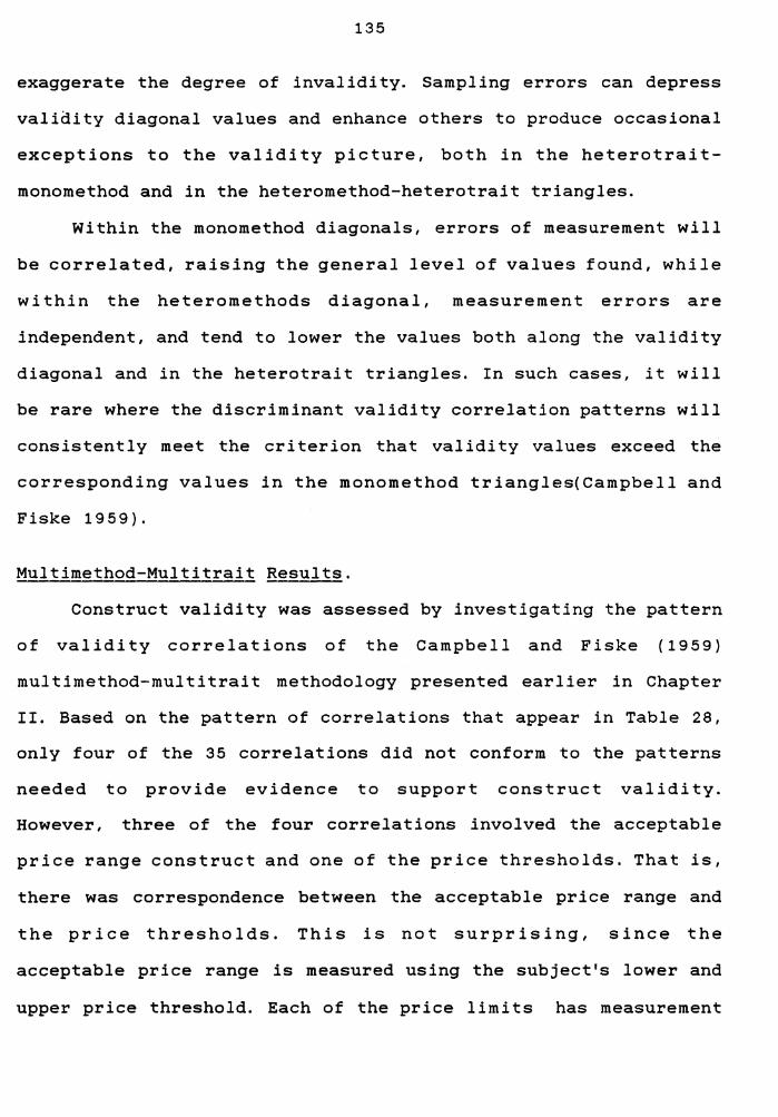
135

exaggerate the degree of invalidity. Sampling errors can depress

validity diagonal values and enhance others to produce occasional

exceptions to the validity picture, both in the heterotrait-

monomethod and in the heteromethod-heterotrait triangles.

Within the monomethod diagonals, errors of measurement will

be correlated, raising the general level of values found, while

within the heteromethods diagonal, measurement errors are

independent, and tend to lower the values both along the validity

diagonal and in the heterotrait triangles. In such cases, it will

be rare where the discriminant validity correlation patterns will

consistently meet the criterion that validity values exceed the

corresponding values in the monomethod triangles(Campbell and

Fiske 1959).

Multimethod-Multitrait Results.

Construct validity was assessed by investigating the pattern

of validity correlations of the Campbell and Fiske (1959)

multimethod-multitrait methodology presented earlier in Chapter

II. Based on the pattern of correlations that appear in Table 28,

only four of the 35 correlations did not conform to the patterns

needed to provide evidence to support construct validity.

However, three of the four correlations involved the acceptable

price range construct and one of the price thresholds. That is,

there was correspondence between the acceptable price range and

the price thresholds. This is not surprising, since the

acceptable price range is measured using the subject's lower and

upper price threshold. Each of the price limits has measurement

136

TABLE 28

PEARSON PRODUCT MOMENT CORRELATIONS AND THE CRITERIA FOR CONVERGENT AND DISCRIMINANT VALIDITY:

MULTITRAIT-MULTIMETHODMATRIX (THREE TRAITS AND TWO METHODS)

Convergent Validity

Correlation Patterns Criteria

( 1 ) r .545>

r .408>

r .278>

0

0

0

The correlations should be statistically significant, greater then zero, and "sufficiently large."

Discriminant Validity

Correlation Pattern

(2) r r r r r .545> .371, .118*, .306,-.043*

r r r r r .408> .371, .208*, .306, .308

r r r 1 r r .278> .118*,.308,-.043*, .208*

( 3 ) r r r r r .545> • 381 I .055*, • 413 I .021*

r r r r r 1 .408> .320, . 381, .336, .413

r r r 1 r r 1 .278> .055*, .320, .021*, .336

Criteria

Differences in correlations should be in the proper direction and statistically significant.

Differences in correlations should be in the proper direction and statistically significant.

137

TABLE 28 (Continued)

(4) Within all heterotrait triangles, the pattern of intertrait correl-lations should be repeated across triangles.

Since r r r Bl Al > Cl Bl > ClAl, the

r r r B2Al > C2Bl > C2Al

r r r B2A2 > C2B2 > C2A2

Using the correlations, then

.381 > .320 > .055*

.306 > .208*>-.043*

.413 > .336 > .021*

.371 > .308 > .118*

Differences in correl-ations should be in the proper direction and statistically significant.

following should hold true

Adapted from Bagozzi 1980, p.131

*CORRELATIONS SIGNIFICANT AT P > 0.10 ALL OTHER CORELATIONS SIGNIFICANT AT P <= 0.031

1 correlations not meeting the pattern

138

error and a trait score. Since the two errors are independent and

uncorrelated, they not only do not cancel out but increase the

measurement error in the acceptable price range scores. Thus, the

corelation for the acceptable price range should be small, and

the validity coefficient would also be smaller.

If all of the correlation patterns are satisfied, then it is

safe to conclude that convergent and discriminant validity have

been achieved. However, when some patterns of correlations are

not satisified, then Campbell and Fiske (1959) suggest a counting

procedure where the number of exceptions to predicted patterns is

determined and compared to that expected by chance.

A sign-test was conducted to determine if the number of

correlations larger than the validity value in its row and column

was less than expected on the null hypothesis that half the

values would be above it. The evidence indicated that the number

of correlations larger than the validity value are less than

would be expected by chance alone (p = .125). Therefore, based on

the Campbell and Fiske (1959) criteria, and the fact that

sampling and measurement error most certainly depressed the

validity coefficients, construct validity could be tentatively

acknowledged for each of the two methods.

While the Campbell and Fiske method provides insights as to

construct validity, their procedure does not "provide criteria

· for determining the degree to which operationalizations measure

concepts, the amount of variance due to trait vs. method, or the

adequacy of an entire MM matrix" (Bagozzi 1980), Therefore, a

more rigorous procedure is available to achieve the above goals

139

the causal modeling approach using structural equations.

The causal modeling approach for assessing construct

validity was conducted. Unfortunately, the Ksi matrix was not

positive definite and subsequent analysis was not possible.

Nonetheless, where there are few departures in the correlation

patterns, construct validity can be tentatively acknowledged.

In sum, there is evidence to support the contention that

buyers adjust their acceptable price range with the introduction

of market price info~mation, but only when subjects use the

Stoetzel method. When establishing their acceptable price range

using the Own-category method there was no change in the price

range. Although the acceptable price range scores were in the

right direction, it would seem that the two methods do not

produce similiar scores as initially hypothesized. The two

methods produced similar lower price threshold scores but

produced different upper price limit scores. The Own-category

method upper limit was higher than the Stoetzel upper price

limit.

Based.on the MTMM criterion for confirming method validity,

the two price threshold methods have been shown to have both

convergent and discriminant validity. However, the Own-category

method produced greater reliable scores for each of the three

traits than did the Stoetzel method.

~hapter Summary

This chapter presented the analyses used to test this

study's hypotheses regarding the effect of market price

140

information on the aceptable price range.

The chapter detailed the preliminary analyses conducted on

the data and outlined the results of the homogeneity of variance

tests for the two-way Anovas performed. Since, the factorials

were non-orthogonal designs three separate two-way Anova

procedures were defined as the most appropriate means for

analyzing the factorial designs. Moreover, the subsequent

analyses of variance was conducted on the full data as well as on

the data after outliers had been deleted.

The specific hypotheses were tested using two-way analysis

of variance and paired t-tests. And the chapter concluded with an

examination of the convergent and discriminant validities of the

two methods used for measuring absolute price thresholds.

CHAPTER V

CONCLUSIONS

The last chapter of this dissertation begins by providing a

brief overview of the study and a discussion of the major

findings. Based on the interpretation of these results, the

significance of the research is examined. Finally, the chapter

concludes with an analysis of the limitations of the research and

a discussion of possible directions for future research.

STUDY OVERVIEW

The overall objectives of this research were (1) to test a

specific proposition derived from prior behavioral research and

from social judgment theory on the effect of market price

information on the acceptable price range and acceptable price

limits, and (2) to determine the construct validity of two

acceptable price limit measurement methods.

Specifically, an examination was made on the effect of

market price information on the width of the acceptable price

range for a high-priced product (personal computer) using two

different methods, the Stoetzel and the Own-category method. The

effects were assessed using a 2 by 2 factorial experiment where

the factors were (1) pretest/no pretest, and (2) market price

information/no market price information. Moreover, the effects

were explored using a Solomon 4-Group research design that

concentrated on the internal validity of the results which allows

for stronger inferences to be made since history, maturation, and

treatment/testing interaction can be assessed should that

141

142

stronger inferences can be made.

Two different price threshold measurement methods were used

to measure price thresholds and acceptable price range. Unlike

previous price threshold research, this study examined the test-

retest reliabilities and the construct validities of the Stoetzel

and Own-category methods through Campbell and Fiske's

multimethod-multitrait procedure.

DISCUSSION OF MAJOR FINDINGS

Overal 1, this research lends additional support to the

conceptual scheme and previous body of research that suggests

that consumers go into a purchase situation with a range of

acceptable prices that they are willing to pay for a product

(e.g., Foulihe 1960; Monroe 1971), and provides some support to

the contention that buyers do not enter a purchase situation with

rigidly formed acceptable price limits, but that individual price

limits are adjusted as subjects accumulate market price knowledge

(Cox 1986).

This research extends price threshold research by

investigating one factor that may influence the price thresholds

and acceptable price range --- market price information, and by

establishing acceptable price limits and acceptable price range

for a relatively high-priced, infrequently purchased product ---

a personal computer. Moreover, by examining the construct

validity of two price threshold measurement methods, this

research provides evidence to eliminate method artifact criticism

of previous price threshold research which used either the

143

Stoetzel or Own-category method.

The results of the experiment were somewhat inconsistent

with the original hypothesis derived from social judgment theory.

~hile the results of the Stoetzel method strongly supported the

hypothesis that the acceptable price range would be narrower for

those subjects in the high involvement treatment (possessing

market price information) than subjects in the low involvement

treatment (little or no market price information), there was no

change in the acceptable price range when the same subjects used

the Own-category method.

The acceptable price range results of the Stoetzel method

confirm the findings of Raju (1977) and Foulihe (1960) who also

used the same method despite the fact that product involvement

was defined differently, and that the products differed in terms

of frequency of purchase and product price category. On the one

hand, Raju (1977) used a stereo receiver that was infrequently

purchased and a relatively high-priced product, and defined

product involvement in terms of (1) past purchase experience, (2)

product knowledge, and (3) product information communicated by

word-of-mouth from friends and others. On the other hand, Foulihe

(1970) used two relatively low-priced products are frequently

purchased products (package soup and laundry detergent), and

included brand/no brand name conditions.

This research improved on the methodological limitations of

the Raju (1977) and Foulihe (1960) studies by concentrating on

internal validity through the use of a more strenuous

experimental design. Moreover, while Raju (1977) and Foulihe

144

(1960) did not control for potential differences in sex and prior

price knowledge of their subjects, this research incorporated

those factors as covariates. The results of the analysis of

covariance did not differ from the original ANOVA findings.

The acceptable price range results using the Own-category

method failed to support the hypothesis. There was no difference

in the width of the acceptable price range between the high and

low involvement (market price knowledge) conditions. This

finding confirmed the findings of Cummings and Ostrum (1982).

Using a different method, they found that there was no change in

the width of the acceptable price range despite manipulating

product involvement and price sensitivity. While Cummings and

Ostrum (1982) did not control for sex and prior-price knowledge

difference among their subjects, these covariates were

investigated in this research. Again, the acceptable price range

results did not differ from the inital ANOVA findings.

As an ancilliary finding, the lower and upper price limit

results, in part, confirm the findings of Cox (1986) who

suggested that buyers do not enter a purchase situation with

rigidly formed acceptable price limits, but that individual price

limits are adjusted as subjects accumulate market price

knowledge.

The lower and upper price limits, as well as the acceptable

price range were significantly different for those subjects that

received market price information than those subjects who

received no price information when the Stoetzel method was used.

145

The mean lower and mean upper price limits were greater for the

subjects receiving the market price information than subjects who

received no market price information. These findings suggest that

subject price thresholds move in the direction of the market

prices. These results are consistent with the Stoetzel method

findings reported by Foulihe (1960) at least in terms of one of

the two branded products he investigated. He reported that the

lower and upper price limits were greater for branded than

unbranded products. However, the results were contrary to the

findings reported by Raju (1977). He reported no difference in

the lower and upper price limits across the involvement

conditions, despite finding a difference in the acceptable price

range.

The lower and upper price limit results of the Own-category

method differed from the Stoetzel results in terms of the upper

price limit. When the Own-category method was used, only the

lower price limit differed across the two information conditions.

The mean lower price limit was greater in the high market price

information condition than in the low price informatiqn

condition. The upper price limit remained unchanged across the

two treatments. These findings are similar to those reported by

Cox (1986) who used the Own-category method in his investigation

of short and long price series. The actual effect sizes for the

lower price limit, upper price limit, and acceptable price range

are outlined in Table 29.

Most importantly, there was a reduction in the lower and

upper price limit variability when market price information was

146

TABLE 29

EFFECTS OF MARKET PRICE INFORMATION

ON THE PRICE RANGE, LOWER PRICE LIMIT, AND UPPER

STOETZEL METHOD (FULL DATA)

VARIABLE EFFECT SIZE "D II

PRICE RANGE -0.414

LOWER PRICE LIMIT +0.781

UPPER PRICE LIMIT +0.087

STOETZEL METHOD (OUTLIERS DELETED)

VARIABLE

PRICE RANGE

LOWER PRICE LIMIT

UPPER PRICE LIMIT

VARIABLE

PRICE RANGE

LOWER PRICE LIMIT

UPPER PRICE LIMIT

EFFECT SIZE

-0.380

+1.002

+0.759

"D II

OWN-CATEGORY METHOD (FULL DATA)

EFFECT SIZE "D"

-0.162

+0.429

+o .125

VARIABLE

PRICE RANGE

OWN-CATEGORY METHOD (OUTLIERS DELETED)

EFFECT SIZE "D"

LOWER PRICE LIMIT

UPPER PRICE LIMIT

-o .151

+0.575

+0.068

PRICE LIMIT

147

introduced. Despite this reduction in variability, there was

greater variability in the upper price limit than in the lower

price limit across both methods. This finding also confirmed the

upper price limit variability results reported by Cox (1986),

Fouilhe (1960), and Raju (1977), despite the differ products and

price levels of the products. While the variability of the upper

limit was greater than that of the lower price limit, the upper

price limit variability was reduced by prior purchase behavior

(Raju 1977), price last paid (Cox 1986), brand name (Fouilhe

1960), and market price information in this study. These findings

would suggest that subjects have difficulty establishing stable

upper price limits where only one informational cue is provided.

This difficulty would be expected. Monroe (1971) did lament the

fact that most pricing research seldom incorporates the types of

information always available to the buyer at point of purchase

such as, price information, physical product, brand name, store

image, etc. Moreover, it is possible that unlike the lower price

limit, the upper price limit has a budget or economic constraint.

An economic constraint contributes to the variability in the

upper price limit.

It would be useful in future studies to try to uncover those

variables which might explain this variability. Such correlates

would not only be interesting in their own right, but they could

be used as covariates to increase the power of the statistical

tests examining the effect of any factors that may effect the

acceptable price range and price limits.

While previous price threshold research supports the notion

148

that consumers enter the market with acceptable prices they are

willing to pay for a specific product, no attempt has been made

to assess the reliability or construct validity of the various

price limit measurement methods. The Stoetzel method has been

criticized by (Monroe 1971) and (Gabor and Granger 1966). They

claim that the relatively simple two-question Stoetzel method

employes leading and biased questions, and that the method allows

no inference to be made concerning price and the willingness to

buy response. Moreover, Stoetzel (1954), himself, questioned what

his method was indeed measuring. The Own-category method derived

from social judgment theory is considered a much better method

primarily because of its.theoretical foundation (Monroe 1971; Cox

1986). Nonetheless, no empirical evidence in terms of reliability

or construct validity of either method has been reported. This

research, however, assessed not only the reliability but also the

construct validity of two specific threshold measurement

procedures, the Stoetzel and Own-category method.

Test-retest reliabilities of the lower and upper price

limits, and the acceptable price range were assessed through

repeated measurement of the subjects in group 2 of the Solomon 4-

group research design. The reliability coefficients weregreater

for the Own-category method than for the Stoetzel method.

This finding may suggest that the methods may differ, and that

difference may be due to the different cognitive processes evoked

by the two methods such that there is instability at the price

limits. However, the Own-category method produced more reliable

149

scores than did the Stoetzel method.

The difference in cognitive processes evoked by the two

methods differ in terms of method involvement. That is, subjects

are more involved in the Own-category method than in the Stoetzel

method. While the Stoetzel method requires subjects to select one

price for their lower price limit and one price for their upper

price limit from among a price series of 50 prices, the Own-

category method requires the subjects to first sort the 50 prices

in terms of similiarity and then label their price groups in

terms of acceptable/unacceptable prices to pay. This procedure

may have overpowered the treatment versus control conditions

since the lowest price in the acceptable price piles is used to

establish the subject's acceptable lower and upper price limit.

This may have absured the true impact of market price knowledge

as hypothesized.

Construct validity in terms of discriminant and convergent

validities of the Stoetzel and Own-category method was assessed

using Campbell and Fiske's multimethod-multitrait matrix of zero

order correlations. The pattern of the validity coefficients

indicated support for both convergent and discriminant validity.

Therefore, the construct validity of the two methods can be

tentatively accepted such that the criticism of the Stoetzel

method may not make a difference in price threshold measurement.

However, more strenuous procedures exist to evaluate construct

validity {Bagozzi 1980). Confirmatory factor analysis and casual

modeling are more informative since trait and method variance can

be assessed. Unfortunately, neither procedure could be used since

150

the model was underidentif ied.

Most importantly, the large number of subjects who could not

establish a singular acceptable price range using the Own-

category method indicates a potential method artifact in the Own-

ca tegory method that does not appear in the Stoetzel method. This

artifact if it exists (it is possible that the results were due

to subjects not understanding the instructions of the Own-

category sorting procedure) does impact on assessing construct

validity. The validity coefficients would be attenuated and would

be greater than those reported in this study. Moreover, it would

make it more difficult to assess the pattern of correlations in

assessing discriminant and convergent validity in terms of the

multitrait-monomethod and multitrait and heterotrait triangles of

the Campbell and Fiske multimethod-multitrait matix.

SIGNIFICANCE OF THE RESEARCH

Research on acceptable price limits and acceptable price

range primarily investigated the hypothesis that buyers possess a

range of acceptable prices that they are willing to pay for a

contemplated purchase that are bounded by a lower and upper price

limit. That is, there are prices that would be considered too low

or too high and a purchase would be less likely to be made.

Moreover, prior research studies have used a number of methods

for assessing acceptable price limits and acceptable price range

but no attempt has been made to assess either the reliabilities

or the construct validities of the methods.

151

Only Raju (1977), Foulihe (1960), and Cummings and Ostrum

(1982) have attempted to investigate acceptable price range

change. While Raju (1977) found that the acceptable price range

narrowed with product involvement, and Foulihe (1960) found that

branded products had narrower price ranges than their unbranded

counterparts, Cummings and Ostrum (1982) found no such change

when subjects differed in purchase involvement. Unfortunately,

these studies did not control for prior price knowledge and used

the Stoetzel procedure which has not been shown to be a valid

measurement method. Moreover, the studies used only products that

were low in price and frequently purchased (this latter factor

could be considered as assuming market price knowledge).

This research extends the acceptable price range research by

assessing the effect of market price information on acceptable

price range and acceptable price limits for a high priced product

using prior-price knowledge and gender as covariates. Further,

the experimental design concentrated on internal validity, unlike

the other studies, such that stronger inferences may be made.

Moreover, acceptable price range and acceptable price limits

were measured through two different methods.

The research makes a major contribution to the literature by

assessing the construct validity of two price threshold

measurement methods. While they were found to be valid measures,

the results of the experiment were conflicting. This would

suggest that there may be different cognitive processes evoked by

the two methods. While market price information narrowed the

acceptable price range for the Stoetzel. method, there was no

152

change in the Own-category acceptable price range. Moreover,

there was greater variability in the acceptable price range and

price limit scores with the Own-category method than with the

Stoetzel method. This finding suggests that consumers may have

more difficulty establishing their upper price limits where price

is the only informational cue available to them.

The most interesting finding of the research in terms of

method used was that while subjects could establish their

acceptable price range and lower and upper price limits without

exception using the Stoetzel method, a large number of the same

subjects could not do so using the Own-category method. Many

subjects had a number of acceptable price ranges along the low to

high price continuum. That is, subjects had acceptable low,

acceptable medium, and acceptable high price ranges they were

willing to pay for a contemplated purchase with various lower and

upper price limits. This finding has neither been reported by

previous price threshold studies using the Own-category method

nor was it present during the pretesting of the instruments.

Moreover, it suggests that the that consumers have a singular

acceptable price range bounded by a lower and upper price limit

for a contemplated purchase may have limitations at least in

terms of a high-priced product. While this is an interesting

supposition, it is equally possible that those subjects who could

not establish a single acceptable price range did not understand

the instructions. However, it is equally possible that given the

number of price stimuli (50) and the price stimulus range ($1600

153

to $6400) that some subjects considered the product in, lieu of

the prices they were asked to evaluate, in terms of different

product offerings.

Based on the findin9s of this research, a singular

acceptable price range may be an appropriate assumption for low-

priced and frequently purchased products (all prior price

threshold research have used relatively low priced and frequently

purchased products with fewer than 30 prices to be evaluated),

but may not be valid when a high-priced and infrequently

purchased product is used. This assumption needs further study

within the context of other subject populations and product

categories using more than one method for price threshold

measurement.

From the managerial perspective, the research supports the

notion that buyers have a range of acceptable prices that they

are willing to pay for a product, and that the potential buyer

may not enter a purchase situation with rigidly formed price

limits within which the buyer is most likely to make a purchase

at least in terms of a relatively high-priced product. Most

importantly, buyers may adjust their acceptable price limits at

the point of purchase. The particular importance of this issue is

that marketing managers may be able to shift buyers• price limits

and acceptable price range by altering their product assortment

or prices (Cox 1986). For example, a retailer can add more

expensive items to their assortment in order to make the item

appear less extravagant to its customers or at least discourage

purchase at the lower price range of the assortment. Moreover,

154

given the large variability in the upper price limit, it would

seem that point of purchase interaction between buyer and seller

may be more important in the final purchase decision at the upper

price range of a product assortment then at the lower price

range. The seller can provide additional information or clarify

product information not available (or at least not known) to the

buyer such that the seller's information may stabilize the upper

price limit and a purchase is more likely to be made. However,

this effect needs to be examined further.

Managers can estimate consumer acceptable price range for

.various products to aid in the initial setting of their product's

price within consumer acceptable price limits to increase the

probability of purchase using two separate methods. Both methods

p·roduce similar lower price limits, but differ with respect to

the upper price limit. The Own-category method produces higher

upper limit scores than does the Stoetzel method.

LIMITATIONS

The major limitations of the research focused on two

factors: (1) threats to validity, and (2) the assumptions

involved in the use of analysis of variance with unequal cell

sizes. These limitations can have a deleterious effect on the

strength of the inferences made, as well as help to qualify the

significance of the research.

155

THREATS TO VALIDITY

In evaluating any experimental design, three decisionshave

to be made concerning the sample data: (1) Is the study sensitive

enough to permit reasonable statements about covariation? (2) If

it is sensitive enough, is there any reasonable evidence from

which to infer that the persumed cause and effect covary? and (3)

if there is such evidence, how strongly do the two variables

covary? These factors, therefore, are concerned with statistical

conclusion validity. A discussion of how threats to these

validities were addressed in this study are presented below.

THREATS TO STATISTICAL CONCLUSION VALIDITY

Lo~ Statistical Po~er. The likelihood that an incorrect no-

dif ference conclusion (Type II error) is made increases when the

sample size is small, alpha level is set low, and the expected

effect size is low. Based on the effect sizes calculated from the

work of Stoetzel ( 1954) and the large ef feet size inferred from

Raju {1977), the effect of product price knowledge on price

thresholds was expected to produce at least a moderate effect

size "D" of 0.40 {Rosenthal, 1980). Based on those considerations

and the smallest sample size (n=56) cell of the various 2 by 2

factorials tested for the experiment, the power of the test on

independent group means in this study was 87 percent {Cohen 1977)

where testing was conducted at p = 0.10. Therefore, the testing

procedure provides sufficient power to minimize type II error.

Statistic~l Assumption~· A two-way analysis of variance was

used to determine the impact of market price information on the

156

acceptable price range and lower and upper price limit. This

testing procedure assumes equal population dispersions or

homogeneity of variances among the groups. The Bartlett-Box F

univariate homogeneity of variance test (Morrison 1976) suggested

that this condition was not satisified. While the violation of

this assumption can distort tests of significance when cell sizes

are unequal, the data was neither transformed nor was any data

randomly deleted to achieve equal cell sizes due to (1) the

magnitude of the degrees of freedom and power of the Bartlett

test, and (2) the results of the less conservation Cochran Q test

which failed to reject the homogeneity assumptions in all cases

save the upper price limit for the Own-category method. The

failure to meet the assumption of equality of variance using

solely Bartlett's test was not considered to have a serious

distortive effect on the tests of significance in light of the

Cochran test results. However, since outliers can distort

analysis of variance tests, statistical analyses were conducted

on the full data as well as on the data where outliers were

deleted.

Unegual Cell Sizes. The analysis of variance conducted on the

factorial design was based on unequal cell counts. Where cells

are unequal the statistical results may be misleading. As a

result, three separate testing procedures were conducted on the

data to determine if the unequal cell sizes were severe enough to

distort the conclusions. However, the results of the three

separate statistical procedures did not differ.

157

!h~ R~li~2ili!Y Qf M~~~~!:~~· The reliability of the price

threshold methods have hitherto not been tested for reliability

in any previous price threshold study. Unreliable measures are

known to inf late standard errors of the estimates and these

standard errors play a crucial role in data interpretation. As

such, Group 2 of the Solomon 4-Group design provided the means

for reliability estimation using the test-retest procedure.

Evaluation of the reliability coefficients indicated that

there was substantial measurement error in both methods. There

was less measurement error in the lower and upper price limit,

and acceptable price range scores in the Own-category method then

in the Stoetzel method. Moreover, the maximum reliability

coefficient was only r = 0.649 for the upper price limit, and

only r = 0.388 for the acceptable price range using the Own-

category method. As a result, the true effect of the experimental

treatment may have been masked particularly in the Own-category

method results, and the validity coefficients were most likely

deflated. Based on measurement theory (Nunnally 1967), a validity

coeff icent can not be greater then the square root of the highest

reliability coefficent. As a result, the validity coeficients can

be expected to be low given the reliability coefficients.

R~li~2ili!Y Qf !!:~~!m~!!! !m12l~m~!!!~!i2!!· Variation in

treatment implementation must be controlled. Otherwise, the lack

of standardization in treatment implementation would inf late

error variance and decrease the probability of experimentally

finding true differences. The measurement procedures, however,

158

were designed to maintain standardization. Moreover, while two

researchers conducted the experiment both were carefully trained

to maintain consistency, and the experimental procedures were

designed to minimize subject-researcher interaction.

Random Irrelevancies in the Experimental Setting. There are

other factors in the experimental setting that can affect scores

on the dependent variables and inf late error variance. This

threat can best be controlled by selecting an experimental

setting as free of extraneous variation as possible. While

finding such a setting is often impossible, the most effective

way to reduce the effects of extraneous variability is to use

experimental procedures which incorporate subject involvement in

the experimental task as well as which direct the subjects to

focus their attention on the treatment (Cook and Campbell 1979).

The research procedures in this study are highly task-

oriented and the open-book quiz on the prices of the price

information treatment draws subject attention to the treatment.

The manipulation check was assessed to determine if subjects

attended to the market price information presented. The results

of the manipulation check indicated that 99.5% of the subjects

correctly identified the lowest price, 98.5% correctly identified

the highest price, and 95.5% correctly identified the number of

different prices presented. However, only 68% corrected

determined the average market price from the market price

information presented ( this is not surprising since subjects had

to estimate the average price from the prices presented without

159

the aid of a calculator). Still, 87% were within $200 of the

average price. These findings would suggest that subjects did

attend to the market price information presented.

As a result of the above, the research design can be

considered as reducing some, but not all, possible effects of

extraneous variation. Of more primary concern was to access the

magnitude of various threats to internal validity that was made

possible by the research design used in this research.

THREATS TO INTERNAL VALIDITY

Since internal validity was the primary concern of this

research, the major alternative explanations of the results are

predicated on the extent that threats to internal validity exist.

The manner in which those threats were addressed in this research

are discussed below.

Demand Artifacts. Subject responses could be influenced by

motives aroused by the fact that the subject is aware of his/her

participation in the research. The subject is not immune to the

fact that {s)he is in a testing situation. Thus, {s)he may infer

the hypotheses under study and attempt to be "good" subjects

(Sawyer, 1977).

Subjects were debriefed based on one question in the

response booklet. Where subjects had guessed the purpose of the

experiment, their response was eliminated from the analysis.

However, subject propensity to be consciously concerned with

guessing the purpose of the study is specious at best. Debriefing

the subjects to determine their knowledge of the research purpose

160

is nothing more than an invitation to offer a guess-estimation.

This P2§! !~£12 questioning itself initiates a cognitive state

that may or may not have existed during the research procedure.

However, no subjects correctly identified the research purpose

and no cases were eliminated from the analysis.

Evaluation Apprehension. This demand artifact concerns the

subject's desire to win a positive evaluation from the researcher

or at least providing no negative evaluation. To minimize the

potential response bias, the subjects were assured of response

confidentiality and were told that group response rather than

individual response was the only concern of the study.

gi§!2~Y !!!~£!· Where there is a potential for events to

occur between the pretest and posttest, the results may be

confounded by those events. Therefore, it becomes difficult to

establish whether the results were due to the treatment or some

other extraneous factor. The Solomon 4-Group design provides a

means for detecting history effects. An estimate of the history,

maturation , and interactive effects are explicated below.

Maturation Effects. In a pretest-posttest design the effects

obtained may not be due solely to the treatment but rather to

changes that may have occurred in the subjects during the period

between the tests. While it is difficult to totally eliminate

this effect, it can be minimized by disguising the research

purpose as well as by minimizing the time frame during which the

two tests occur. As such, the two test periods were held just

five days apart.

161

Interactive Effect. With a pretest-posttest research design,

there is the possibility of an interaction effect due to possible

pretest subject sensitization. The Solomon design presents a 2 by

2 factorial analysis of variance to assess this interactive

effect. Based on the statistical analysis of the factorials for

each of the dependent variables for each method, the interactive

effect was not found to be significant.

Q~g~~ ~12~· The research did not consider the impact of

order bias. That is, the effect on the dependent variables of the

two methods by the order that the methods were presented to the

subjects. The two methods do differ in terms of application. The

Own-category method was more time consuming and may initiate

greater cognitive effort than the Stoetzel method. Recall that

the Stoetzel method makes use of two simple questions from which

the acceptable price range, and lower and upper price limit is

determined. However, the Own-category method requires greater

subject involvement because of the extensive sorting procedure.

The difference in the two methods can be more dramatically

presented in terms of time. The experiment was conducted over a

period of one and one-half hours. The researchers conducted a

visual assessment of the time consumed by the subjects using both

methods. The Stoetzel method required approximately 10 minutes of

the subjects time, while the Own-category method consumed almost

one hour of the allocated testing period. As a result, it is

possible that fatique may have distorted the Own-category

findings. However, there was no reason to believe that subjects

became tired during the sorting procedure. Most importantly, the

162

Own-category method produced more reliable price limit and

acceptable price range scores than did the Stoetzel method. This

finding would seem to counter the fatique limitation in that one

would expect that fatigue would promote less reliability for the

method that required more cognitive and physical effort.

In all cases, the Stoetzel method was used by the subjects

first, and the Own-category method second. Whether there is an

order effect was not determined, but should be addressed in

future price threshold research.

~~l~£!!2n ~!~~· Selection bias is a threat when an effect

may be due to the differences in subjects within groups than

between groups. To counter this threat, subjects were randomly

assigned to the different experimental groups. Randomly assigning

subjects is viewed as producing probabilistically equivalent

groups (Kerlinger 1973). However, given the large degree of non-

participation by subjects over the two phases it is reasonable to

question whether the groups were indeed statistically equivalent

despite the statistical support of the Cochran C homogeneity of

variance test.

Mortality Effects. Pretest-posttest designs are subject to

selection artifact criticism. It was expected that some subjects

who were randomly selected to participate during both sessions

would not participate during the second phase of the study. Thus,

the effect may be due to the kinds of people who dropped oµt of

the experiment. Where this occurs, the resultant experimental

groups may no longer be considered as statistically equivalent.

163

In hopes of reducing the mortality rate, all subjects were

given an incentive to participate in the entire study. All

subjects received bonus marks in their commerce course for

participating in the experiment. Those subjects who were assigned

to participate in both phases of the study were told by their

professors that they had to participate in both phases of the

study to receive their participation marks.

Despite these precautions, there was a larger than expected

mortality rate as discussed in Chapter III. It is possible that

those subjects who did not participate may have been different

from those-who did participate. Thus, non-participants may have

increased within-group variability and reduced the power of the

testing procedure. Possibly, the non-participating subjects may

have masked the true effect of the market price information

treatment. This subject mortality may have distorted the results

of the Own-category method.

EFFECTS OP EXTRAHEOUS VARIABILITY

The Solomon 4-group design is considered a classic research

design because it provides a means to assess the extent of

extraneous variability in pretest-posttest experimental setting,

and to determine the true impact of the experimental stimulus.

Before assessing the impact of extraneous variability in the

experiment, the manner in which this variability was determined

is presented. The quantitative assessment is based on the

formulae outlined by Churchill (1983, p.99-101).

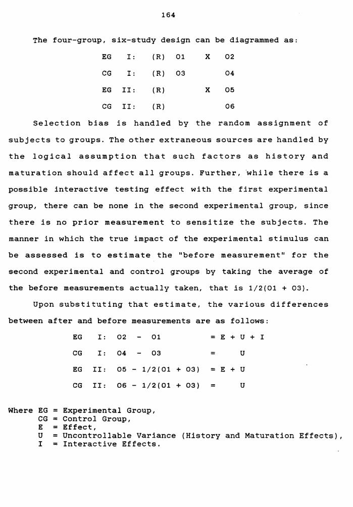
164

The four-group, six-study design can be diagrammed as:

EG I:

CG I:

EG II:

CG II:

(R) 01

(R) 03

x

(R) X

( R)

02

04

05

06

Selection bias is handled by the random assignment of

subjects to groups. The other extraneous sources are handled by

the logical assumption that such factors as history and

maturation should affect all groups. Further, ~hile there is a

possible interactive testing effect with the first experimental

group, there can be none in the second experimental group, since

there is no prior measurement to sensitize the subjects. The

manner in which the true impact of the experimental stimulus can

be assessed is to estimate the "before measurement" for the

second experimental and control groups by taking the average of

the before measurements actually taken, that is 1/2(01 + 03).

Upon substituting that estimate, the various differences

between after and before measurements are as follows:

Where EG CG E u I

EG I: 02 01 = E + U + I

CG I: 04 03 = u

EG II: 05 - 1/2(01 + 03) = E + U

CG II: 06 - 1/2(01 + 03) = U

= Experimental Group, = Control Group, = Effect, = Uncontrollable Variance = Interactive Effects.

(History and Maturation Effects),

165

The impact of the experimental stimulus can be determined by

comparing the second experimental and control groups and is given

in the following calculation:

[05 - 1/2(01 - 03)] - [06 - 1/2(01 - 03)] = [E + U] - [U] = E

Not only does the design allow the uncontrolled extraneous

factors to be estimated, but also provides an estimate of the

interactive testing effect. An estimate of the interactive

testing effect is provided by comparing experimental groups I and

II through the calculation:

[02 - 01] - [05 - 1/2(01 + 03)] = [ E + U +I] - [E + U] =I

!~pact of Uncontrollable Variance. The data was subjected to

the calculations as mentioned above for each of the independent

variables and for each of the two methods. It should be noted

that history and maturation effects can not be separately

assessed through the calculations and must be assessed in totem.

However, the Solomon design provides two separate estimates of

the uncontrollable variance. These estimates are calculated from

CG I and CG II of the design presented above. The data was tested

using t-tests. The statistical summary of the results are

outlined in Appendix F.

Stoetzel Results. For the Stoetzel method lower price limit,

the estimates of the uncontrollable history and maturation

effects were found to be statistically insignificant. The two

uncontrollable variance estimates were x=0.268 (s.d.=5.494) and

166

x=0.254 (s.d.=7.257). The uncontrollable variance was also found

to be insignificant for the upper price limit. The two mean

estimates of the uncontrolled variance were x=0.750 (s.d=6.837),

and x=0.541 (s.d.=7.326). The effect of the uncontrollable

variance on the acceptable price range was also found to be

insignificant. The estimates were x=0.464 (s.d.= 6.114), and

x=0.216 (s.d.= 6.989).

Overall, there was no evidence to

uncontrollable variance primarily in terms

maturation variance masked the experimental

suggest that

of history and

effects in the

Stoetzel method. Moreover, as detailed in Chapter 4, no

significant interactive testing effect was uncovered.

!h§! Q~!!=.£§!.!§!gQ!:Y B§!.§.!!!.!.§.· With the Own-category method,

the estimates of the uncontrollable history and maturation

effects for the lower price limit were found to be statistically

insignificant. The two uncontrollable variance estimates were

x=0.625 (s.d.=5.214) and x= -0.590 (s.d.= 6.203). The

uncontrollable variance was also found to be insignificant for

the upper price limit. The two mean estimates of the variance

were x=0.073 (s.d=5.727), and x=0.149 (s.d.= 5.837). There was

also an insignificant effect of uncontrollable variance on the

acceptable price range. The estimates were x=0.230 (s.d.= 6.102),

and x=0 .. 089 (s.d=7.002).

Overall, there was no evidence to suggest that

uncontrollable variance in terms of history and maturation

variance effected or masked the experimental effects for the Own-

167

category method. Moreover, as detailed in Chapter 4, no

significant interactive testing effect was uncovered.

In sum, the major limitations of the studyencompass both

external and internal validity issues. The manner in which

internal validity concerns were addressed were presented above.

However, no attention was paid to the external validity of the

study. Since the primary purpose of this study was to test

theory, the research design concentrated on improving internal

validity. Concerns for internal validity adversely affects

external validity or the extent to which the results can be

generalized to and across different types of subjects, settings,

and times. Therfore, there was no attempt to generalize the

results beyond the initial setting, time, subjects, and products.

A further limitation of the study is that it does not

incorporate other factors or information that a subject may bring

into a purchase situation. While only market price information

was manipulated, other informational cues may also impact on the

acceptable price range and price limits. For example, Foulihe

(1960) found that brand name narrowed the acceptable price range,

although no statistical evidence was presented to support that

contention. Nonetheless, brand name is also an informational cue

that is always available to a buyer prior to and at the point of

purchase. Brand name was not manipulated in this research.

Moreover, prior purchase experience, product knowledge, store and

product image are but a few of the potential factors that may

impact on the acceptable price range and acceptable price limits.

These factors were not manipulated in the study.

168

FUTURE RESEARCH

As in the case of most marketing research, this research

generates more questions than it answered. There ar~ other

factors other than market price knowledge that effect price

thresholds and acceptable price range. One such factor is

consumer involvement - both with the particular product class and

with prices in general. Research in general ( Sherif and Hovland

1961; Sherif et al. 1965) has indicated that subjects who are

involved with a class of stimulus are likely to consider a

narrower latitude of stimulus as acceptable. This suggests that

the more information accumulated prior to a purchase situation

the more discriminating the buyer becomes in assessing what

prices are acceptable and unacceptable to consider paying for a

product. Unfortunately, prior research (Raju 1977; Cummings and

O•trum 1982), as well as this research, can not support the

notion that they indeed measured product involvement. Future

research should attempt to use a valid measure to measure product

involvement. Such a study would enhance the hypothesis of the

effect of product involvement which encompasses more than just

prior price knowledge on the acceptable price range and the price

limits. It is also possible that there may be demographic (e.g.,

gender, age, etc.) and behavioral (e.g., prior purchase

experience, product price category, prior information search)

factors which either directly or indirectly effect consumer price

limits and acceptable price range. Both of these factors may be

used to more clearly define product involvement and lead to a

169

more indepth investigation of product involvement effect on the

acceptable price range. This research only considers product

involvement in terms of market price knowledge on the acceptable

price limits.

There have been four different methods that have measured

acceptable price limits, and this research validated two of the

four methods. The Stoetzel method was a simple and quick method

to assess acceptable price limits, while the Own-category method

was more complex and more time-consuming. Both methods produced

similar lower price limit scores but produced different upper

price limit scores. Moreover, the upper price limits witnessed

more variability than the lower price limit. Future research

should investigate tha nature of the variability in the upper

price limit. Such research would identify potential covariates

and thus increase the power of the testing procedures such that

theoretically generated hypotheses should be confirmed and

conflicting experimental results should be easily identified.

This would lead to more powerful tests of the theoretical

hypotheses, and aid in identifying where and under what

conditions researchers should concentrate their efforts.

Furthermore, such research would lead to the identification of

possible method artifacts.

Future studies should test the generalizability of these

findings, by examining other subject populations (other than

students) and product/price categories, and by increasing the

realism of the task --- presenting actual products and asking

170

subjects to make actual purchase commitments (Cox 1986).

The reliability and construct validity of the Gabor and

Granger (1966) and the Monroe and Vankatesan (1969) method should

also be assessed. At least three, if not all four methods should

be compared to determine which method or methods should be used

to investigate the aforementioned factors potentially effecting

acceptable price range and price limits. By using at least three

of the methods, reliability and construct validity can be

assessed using the more strenuous causal modeling and

confirmatory factor analysis procedures.

The use of multiple methods makes a major methodological

contribution. At best, each method will have been shown to be

val id and each method can be compared to identify each method's

piccadillos; at worst, certain methods can be shown to be invalid

and allows future researchers to identify contradictions and

conficting evidence concerning price threshold theory within the

realm of method validity. Only under such conditions will the

Marketing discipline progress. Until such time that marketing

academics assess the validity of the methods that they use to

measure any theoretical construct no hypothesis predicated on the

strength of sound theory can be confirmed.

Chapter Summary

The final chapter of this dissertation presents a short

overview of the research and details the research findings in

light of previous price threshold research. The significance of

the research in terms of furthering marketing knowledge and

171

practical knowledge is explicated and the limitations of the

research in terms of internal and external validity are

identified. Moreover, the impact of various uncontrollable

variance within the context of the research design are

investtigated. The chapter concludes with suggests for various

directions for future research.

The overall conclusion is that buyers' acceptable price

ranges differ based on the extend of product price knowledge they

possess. The acceptable price range is narrower for those buyers

who have market price knowledge than those who possess little if

any market price knowledge. However, this finding was supported

only when the acceptable price range was assessed using the

Stoetzel method. The acceptable price range did not differ with

the introduction of market price information in the Own-category

method. Moreover, the Stoetzel and Own-category methods were

found to be valid measures of acceptable price range, and price

limits.

REFERENCES

Adam, Daniel (1958), Les reactions du consommatuer devant le prix: Contribution aux etudes de comportement Societe d'Edition d'Enseignment Superieur.

Bagozzi, Richard P. (1980), Causal Models in Marketing New York: John Wiley & Sons, Inc.

Barnett, V., and T. Lewis (1978), Outliers in Statistical Data, New York: John Wiley & Sons, Inc.

Calder, Bobby J., Lynn W. Phillips, Alice M. Tybout (1981), "Designing Research for Applications," Journal of Consumer Research, 8 (September), 197-207.

Calder, Bobby J., Lynn w. Phillips, Alice M. Tybout (1982), "The Concept of External Validity." Journal of Consumer Research, 9 (December), 240-244.

Calder, Bobby J., Lynn W. Phillips, Alice M. Tybout (1983), "Beyond External Validity," Journal of Consumer Research , 10 (June), 109-111.

Campbell, D. criminant Matrix,"

T., and D. W. Fiske (1959), "Convergent and Dis-Validation by the Multitrait - Multimethod

psychological Bulletin , 56, 81-105.

Churchill, G. A. (1979), 11 A Paradigm for Developing Better Measures for Marketing Constructs," Journal of Marketing Research, XVI (February), 64-73.

(1983), Marketing Research: Methodological Foundations, 3rd. ed., New York: Dryden Press.

Cohen, Jacob (1977), Statistical Power Analysis for the Behaviorial Sciences , New York: Academic Press, Inc.

Cook, Thomas D. and Donald T Campbell (1979), Quasi-Experimentation: Design and Analysis Issues for Field Studies, Chicago: Rand McNally College Publishing Company.

Cooley, William w. and Paul R. Lohnes (1971), Multivariate Data Analysis , New York: John Wiley & Sons, Inc.

Corso, John ( 1963) , 11 A Threshold Concept," 356- 70.

Theoretical-Historical Review Psychological Bulletin , 60

of the (July) I

Cox, Anothony D. (1986), "New Evidence Concerning Consumer Price Limits", Advances in Consumer Research< ed. R. Lutz, 13 (Provo, VT.: Association for Consumer Research), 268-271.

172

173

/, .-,/Cummings, William T and Lonnie L. Ostrom ( 1982), "Measuring Price

Thresholds Using Social Judgment Theory" Journal of the Academy of Marketing Science, Fall, 10, 4 , 395-408.

Daniel, c. (1960), "Locating Outliers in Factorial Experiments," Technometrics , 2, 149-156.

Day, George Change" Behavior: Hall,!nc.

S. (1973), "Theories in S. Ward and T.

Theoretical Sources,

of Attitude Structure and Robertson (eds.), Consumer

Englewood Cliffs: Prentice

,,. ''Deering, B.J. and :J. :Jacoby (1972), "Price Intervals and Individ-

ual Price Limits as Determinants of Product Evaluation and Selection," Proceedings , Third Annual Conference of the Association for Consumer Research, 145-66.

((

Dickson, Peter R. and Alan G. Sawyer (1986), "Point of Purchase Behavior and Perceptions of Supermarket Shoppers," Advances in Consumer Research, ed. Richard Lutz, 13, (Provo,Vt.: Association of Consumer Research), 600-06.

Downey, Susan Lynn (1973), "An Exploratory Investigation of Price as a Function of Latitudes

Unpublished Masters Thesis , University Perception Acceptance", Massachusetts.

into of of

Engel, G. and A. Parducci (1961), "Value of Background in the Specification of the stimulus for :Judgment," :Journal of fsychology, 74, 569-75.

Fouilhe, Pierre (1960), "Evaluation Subjective des prix," Revue Francaise de Sociologie , 1, 163-72.

Gabor, Andre and C.W.:J. Granger (1961), "On the Price Conscious-ness of Consumers," Applied Statistics 10 (November), 170-88.

( 1964), "Price Sensi ti vi ty of the Consumer," :Journal of Advertising Research, 4 (December), 40-44.

(1966), on an Enquiry,"

"Price As an Indicator of Quality: Economica, (February), 43-70.

Report

(1970), "The Attitude of the Consumer to Prices," in B. Taylor and G.Wills, eds., Price Strategy, Princeton: Brandon/Systems Press, 132-51.

Gardner, David M. ( 1977) , "The Role of Consumer Choice, 11 in Selected Aspects of Consumer Behavior, 415-33.

Heller, R. M. Marketing,"

and M. L. Ray (1972), "Measure Validation in :Journal of Marketing Research , 1972, 9, 361-70.

174

Helson, Harry (1964), Adaptation-Level Theory, New York: Harper and Row.

Hovland c. I., I.L. Janis, and H.H. Kelly (1953), Communication and Persuasion, New Haven: Yale University Press.

Jacoby, Jacob Review,"

(1978), "Consumer Research: A State of the Journal of Marketing, 42 (April), 87-96.

Art

Kerlinger, Fred N. (1973), Foundations of Behavioral Research, New York: Holt, Rinehart and Winston, Inc.

Kirk, R. (1968), Experimental Design: Procedures for the Behavioral Sciences , Belmont, Ca.: Brooks, Inc.

Lynch, John G. Jr. (1982), "On the Experiments in Consumer Research," Research , 9 (December), 225-239.

External Journal

Validity of of Consumer

(1983}, "The Role of External Validity in Theoretical Research," Journal of Consumer Research 10 (June), 109-111.

Marsh, B. and A. Parducci (1977), "Natural Anchoring at the Neutral Point of Category Rating Scales," Journal of Experimental and Social Psychology, 60, 1-25.

Monroe, Kent B. (1971), "The Measurement of Price Psychophysics and Lattitudes of Accept~nce," Marketing, 8 (November), 460-4.

Thresholds: Journal of

(1973), "Buyers' Subjective Perception of Price," Journal of Marketing Research, 10 (February}, 70-80.

(1976), Brand Familiarity Consumer Research ,

"The Influence of Price Difference on Brand Preferences," Journal

3 (June), 42-49.

and of

(1979), Pricing: Making Profitable Decisions, New York: McGraw-Hill.

and M. Venkatesan (1969), "The Concept of Price Limits and Psychophysical Measurement: A Laboratory Experiment," Proceedings, Fall Conference American Marketing Association, (August), 345-351. t

and Susan M. Petroshius (1981), "Buyers'Sub-jective Perceptions of Price: An Update of the Evidence", in Tom Robertson and Harold Kassarjian, eds., Perspectives in Consumer Behavior , 3rd. ed., Glendale, Illinois: Scott, Breman and co., 43-55.

175

Christine P. Powell and Pravat K. Choudhury (1986), "Recall versus Recognition as a Measure of Price Awareness," Advances in Consumer Research, ed. Richard Lutz, 13 (Provo, Vt.: Association for Consumer Research), 594-599.

Morrison, New

D. F. (1976), York: McGraw Hill.

Multivariate Statistical Methods,

Nunnally, Jum c. (1967), Psychometric Theory, New York: McGraw Hill Book Company.

Overall, J. E., and D. K. Spiegel (1969), "Concerning Least Analysis of Experimental Data," Psychological 72, 311-322.

Squares Bulletin,

I Parducci, A. (1954),

Single Stimului, March, 169-178.

"Learning Journal

Variables in the Judgement of of Experimental Psychology,

(1956), "Direction of Shift in the Judgment of Single Stimuli, "Journal of Experimental Psychology, March, 169-178.

and R. Hohle (1957), "Restriction of Range in the Judgement of Single Stimuli," American Journal of Psychology, 70, 272-275.

and B. Perrett (1971), "Category Rationing Scales: Effects of Relative Spacing and Frequency of Stimulus Values," Journal of Experimental Psychology, Monograph, 89, 427-52.

Peter. J. Paul (1979), "Reliability: A Review of Psychometric Basics and Recent Marketing Practices, Journal of Marketing Research, XVI (February), 6-17.

(1981), "Construct Validity: A Review of Basis Issues and Marketing Practices," Journal of Marketing Research , XVIII (May), 133-145.

Petroshius, Susan M. (1983), "An Experimental Investigation of the Product Line Pricing Characteristics on Product Evalua-tions", Unpublished Dissertation, Virginia Polytechnic Institute.

Pillemer, David B. and Richard J. Light (1980), "Synthesizing Outcomes: How to use Research Evidence from Many Studies," Harvard Educational Review, 50 (May), 176-95.

I • I RaJU, P.

Price ed •I

S. (1977), "Project Familiarity, Brand Familiarity and Influences on Product Evaluations," in W. Perreault,

Advances in Consumer Research., IV, 64-71.

176

Rosenthal, Robert (1980), "Summarizing Significance Levels," New Directions for Methodology of Social and Behavioral Science, 5, 33-46.

Sawyer, Allen (1977), "Demand Artifacts in Laboratory Experiments in Consumer Research," Journal of Consumer Research 1 (March), 20-30.

Sherif, Carolyn (1963), "Sccial Categorization as a Function of Latitudes of Acceptance and Series Range," Journal of Abnormal and Social Psychology , 48. (February), 148-156.

Sherif, Musafer and Carl I Hovland (1961), Social Judgment: Assimilation and Contrast Effects in Communications and Attitude Change , New Haven, Ct.: Yale University Press.

c. ~herif and R. Negergall (1965), Attitude and Attitude Chang~. Philadelphia: W. B. Saunders Co.

Spector, P. E. (1980), "Techniques for Handling Nonorthogonal Analysis of Variance," Evaluation Review , 4, 843-855.

Speed, F. M., Hocking, R.R., and O. P. Hackney (1978), "Methods of Analysis of Linear Models with Unbalanced Data, "Journal of the American Statistical Association, 73, 105~112.

Stoetzel, Jean (1954), "Le prix comme limits," in P.L. Reynaud, ed., La Psychologie Economique , Paris, _184-88.

Talyor, Bernard .and Gordon Wills (1970), Pricing Strategy, Princeton: Brandon Systems Press.

Tull, D. S. and D. I. Hawkins ( 1.980) , .Marketing Researq!l , 2nd. ed., New York: MacMillian.

Webb, E. (1961), Psychologist ,

"Weber's Law and Consumer Prices," 16 (July) I 450 •

American

Winer, b. J. ( 1971) ...... Statistical Principles in Experimental Design, 2ed., New·York: McGraw-Hill.

APPENDIX A

177

178

STUDENT NAME

STUDENT NUMBER

RESPONSE BOOKLET Sl

179

---Page 1---

INSTRUCTIONS

On your desk should be an instruction booklet and an envelope. When the researcher tells you to begin, turn to page 2 of the instruction booklet. There you will find a product description and a list of prices that you are requested to evaluate. Assume you are interested in buying that product and read the description of the product.

After you have read the product description, you will be given a series of prices that you are requested to evaluate individually in terms of what you would honestly be willing to pay for the product as described. You will be asked to answer two questions based on your price evaluations.

Are these instructions clear? If not, raise your hand.

In a moment we will begin. Remember, you must:

(1) turn to page 2 of the instruction booklet and read the product description.

(2) assume that you are interested in purchasing the product and evaluate the prices that are presented as honestly as possible.

PLEASE DO NOT TURN THE PAGE UNTIL INSTRUCTED TO DO SO

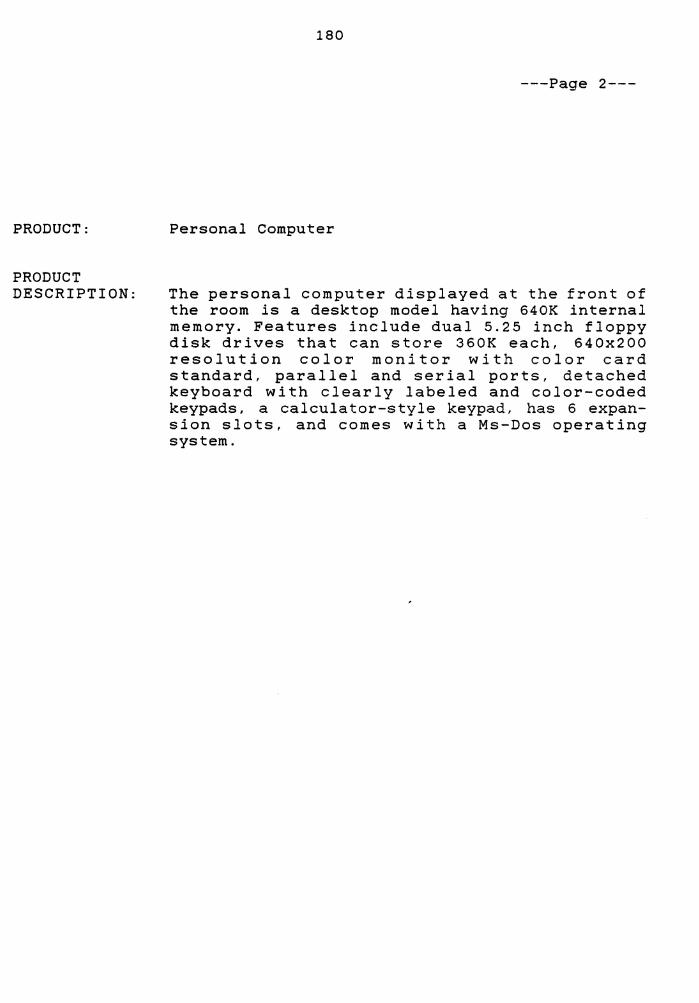
PRODUCT:

PRODUCT DESCRIPTION:

180

---Page 2---

Personal Computer

The personal computer displayed at the front of the room is a desktop model having 640K internal memory. Features include dual 5.25 inch floppy disk drives that can store 360K each, 640x200 resolution color monitor with color card standard, parallel and serial ports, detached keyboard with clearly labeled and color-coded keypads, a calculator-style keypad, has 6 expan-sion slots, and comes with a Ms-Dos operating system.

181

---Page 3---

Prices: $4900,$3600,$2700,$5000,$5900,$5700,$5300,$6000,$4600, $2600,$5400,$3000,$4700,$1900,$2900,$4800,$5800,$3400, $4500,$1600,$43C0,$5200,$4200.$2500,$5500,$1500,$3500, $5600,$3700,$1800,$2400,$1700,$2100,$3800,$3900.$2800, $3100,$6100,$6400,$2200,$6300,$5100,$4400,$3200,$4000, $4100,$2000,$3300,$6200,$2300

1). What is the minimium Erice that you would be willing to pay for this product (that is, below what price would you seriously doubt the quality of the product?)

2) What is the maximium Erice that you would be willing to pay for this product (that is, beyond what price do you feel it would not be worth paying more?)

After you have completed this task, please put your pen or pencil down and await further instructions from the researcher.

PLEASE DO NOT TURN THE PAGE UNTIL INSTRUCTED TO DO SO

182

---Page 4---PLEASE ANSWER THE FOLLOWING QUESTIONS.

1. Have you shopped for a personal computer in the past six months?

] YES

[ ] NO

2. Have you purchased a personal computer in the past six months?

[ ] YES (continue with question 3)

[ ] NO (go to question 6)

3. As best as you can recall, how many different brands or models did you examine?

4. How important was price in your initial purchase decision?

[ ] VERY IMPORTANT

[ ] SOMEWHAT IMPORTANT

[ ] SOMEWHAT UNIMPORTANT

[ ] NOT IMPORTANT

5. How important was price in your final purchase decision?

[ ] VERY IMPORTANT

[ ] SOMEWHAT IMPORTANT

[ SOMEWHAT UNIMPORTANT

[ ] NOT IMPORTANT

6. In the preceding task, did you consider any of the prices as unacceptable?

[ ] YES (continue with question 7)

[ NO (go to question 8)

183

---Page 5---

7. Why were those prices unacceptable? ( List as many reasons as you wish).

8. How knowledgeable would you say you are about the prices of personal computers?

[ ] VERY KNOWLEDGEABLE

[ ] SOMEWHAT KNOWLEDGEABLE

] SOMEWHAT UNKNOWLEDGEABLE

( ] NOT KNOWLEDGEABLE

9. What do you think the investigator is interested in determining from this study?

AFTER COMPLETING THIS BOOKLET, PLEASE PLACE THE BOOKLET IN THE ENVELOPE AND RAISE YOUR HAND TO INDICATE THAT YOU HAVE COMPLETED THIS PART OF THE RESEARCH STUDY.

THANK YOU FOR YOUR COOPERATIOH.

'VS!

S: XIGN:3:ddV

185

STUDENT NAME

STUDENT NUMBER ~~~~~~~~~~-

RESPONSE BOOKLET 01

186

---Page 1---

INSTRUCTIONS

On your desk should be an instruction booklet and an envelope. When the researcher tells you to begin, turn to page 2 of the instruction booklet. There you will find a product description. Assume you are interested in buying that product and read the description.

After you have read the product description empty the envelope and note its contents. These "PRICE CARDS" represent different price offerings for the product. The objective is to sort out the prices into a number of piles you choose. Decide on the piles on the basis of which prices (CARDS) seem to belong together. You may use as many piles as you wish. Do not be concerned about how many piles you create. If you change your mind about any of the prices you have placed in any of the piles, please feel free to rearrange the prices.

After you have finished placing the prices in as many or as few piles as you like put your pen or pencil down and look up to indicate that you have completed the task. Do NOT turn the page of your instruction booklet.

Are these instructions clear? If not, raise your hand.

In a moment we will begin. Remember, you must:

(1) turn to page 2 of the instruction booklet and read the product description.

(2) empty the contents of the envelope and sort the price cards into as many or as few piles as you choose.

PLEASE DO NOT TURN THE PAGE UNTIL INSTRUCTED TO DO SO

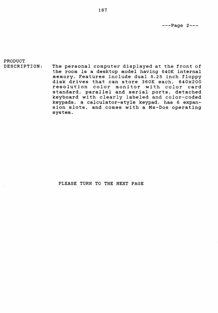
PRODUCT DESCRIPTION:

187

---Page 2---

The personal computer displayed at the front of the room is a desktop model having 640K internal memory. Features include dual 5.25 inch floppy disk drives that can store 360K each, 640x200 resolution color monitor with color card standard, parallel and serial ports, detached keyboard with clearly labeled and color-coded keypads, a calculator-style keypad, has 6 expan-sion slots, and comes with a Ms-Dos operating system.

PLEASE TURN TO THE NEXT PAGE

188

---Page 3---

INSTRUCTIONS --- 2

On the desk in front of you should be the price cards in the pile or piles that you have c~eated. If the pile or piles of price cards contain prices that are ACCEPTABLE to you (that you would be willing to pay for this product), you are requested to put the pile or piles of prices on the left side of the desk. When this is completed, if there is a pile or piles of prices that are UNACCEPTABLE to you put them on the right side of your desk. Lastly, put any pile or piles of prices that may be NEITHER ACCEPTABLE NOR UNACCEPTABLE to you in the center of your desk.

Feel free to rearrange any price cards or piles of prices that you wish.

When this task is completed look straight ahead so the researcher will know you are finished.

Are the instructions clear? If not, raise your hand.

PLEASE DO NOT TURN THE PAGE UNTIL INSTRUCTED TO DO SO

189

---Page 4---

INSTRUCTIONS --- 3

You should now have the price cards arranged on the left, right and/or center of your desk along with a second envelope, Open the envelope and note its contents. Inside the envelope should be some paper clips and two sets of seven "LABEL CARDS" for naming the piles you have created into categories. Read the labels.

Your task is to label the pile or piles of price cards that are on your desk. You may use as many or as few of the labels as you wish but each pile of price cards must have a label. When you have decided which label to use for a particular pile, put that label card on top of the piles of prices that you have selected. Continue until all the piles of price cards have labels. When you have completed this task examine the price cards again to make sure you like where they are. If you don't like where they are you may rearrange any price cards or piles of prices, and relabel the pile.

When all the piles of price cards have label cards on them put a paper clip on each pile. Then put the clipped piles of price cards and any unused label cards back in one of the envelopes.

When this task is completed, please turn the page and answer the questions.

190

---Page 5---

PLEASE ANSWER THE FOLLOWING QUESTIONS.

1. Have you shopped for a personal computer in the past six months?

[ ] YES

[ ] NO

2. Have you purchased a personal computer in the past six months?

[ YES (continue with question 3)

[ ] NO (go to question 6)

3. As best as you can recall, how many different brands or models did you examine?

4. How important was price in your initial purchase decision?

[ ] VERY IMPORTANT

[ ] SOMEWHAT IMPORTANT

[ SOMEWHAT UNIMPORTANT

[ ] NOT IMPORTANT

5. How important was price in your final purchase decision?

[ ] VERY IMPORTANT

[ ] SOMEWHAT IMPORTANT

[ ] SOMEWHAT UNIMPORTANT

[ ] NOT IMPORTANT

6. In the preceding task, did you consider any of the prices as unacceptable?

[ ] YES (continue with question 7)

[ ] NO (go to question 8)

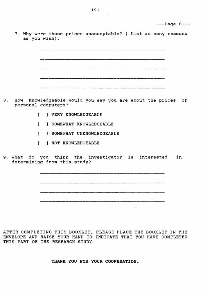
191

---Page 6---

7. Why were those prices unacceptable? ( List as many reasons as you wish) .

8. How knowledgeable would you say you are about the prices of personal computers?

VERY KNOWLEDGEABLE

) SOMEWHAT KNOWLEDGEABLE

) SOMEWHAT UNKNOWLEDGEABLE

[ ) NOT KNOWLEDGEABLE

9. What do you think the investigator is interested in determining from this study?

AFTER COMPLETING THIS BOOKLET, PLEASE PLACE THE BOOKLET IN THE ENVELOPE AND RAISE YOUR HAND TO INDICATE THAT YOU HAVE COMPLETED THIS PART OF THE RESEARCH STUDY.

THANK YOU FOR YOUR COOPERATION.

APPENDIX C

192

193

STUDENT NAME

STUDENT NUMBER

RESPONSE BOOKLET S2

194

---Page 1---

INSTRUCTIONS

On your desk should be an instruction booklet and an envelope. When the researcher tells you to begin, turn to page 2 of the instruction booklet. '!.'here you will find a product description and a list of retail prices that the product is selling for in the Hamilton area. Assume you are interested in buying that product and read the description of the product.

After you have read the product description and reviewed the local retail prices for the product, you will be given a series of prices that you are requested to evaluate individually in terms of what you would honestly be willing to pay for the product as described. You will be asked to answer two questions based on your price evaluations.

Are these instructions clear? If not, raise your hand.

In a moment we will begin. Remember, you must:

(1) turn to page 2 of the instruction booklet and read the product description.

(2) assume that you are interested in purchasing the product and evaluate the prices that are presented as honestly as possible.

PLEASE DO NOT TURK THE PAGE UNTIL INSTRUCTED TO DO SO

PRODUCT:

PRODUCT DESCRIPTION:

195

---Page 2---

Personal Computer

The personal computer displayed at the front of the room is a desktop model having 640K internal memory. Features include dual 5.25 inch floppy disk drives that can store 360K each, 640x200 resolution color monitor with color card standard, parallel and serial ports, detached keyboard with clearly labeled and color-coded keypads, a calculator-style keypad, has 6 expan-sion slots, and comes with a Ms-Dos operating system.

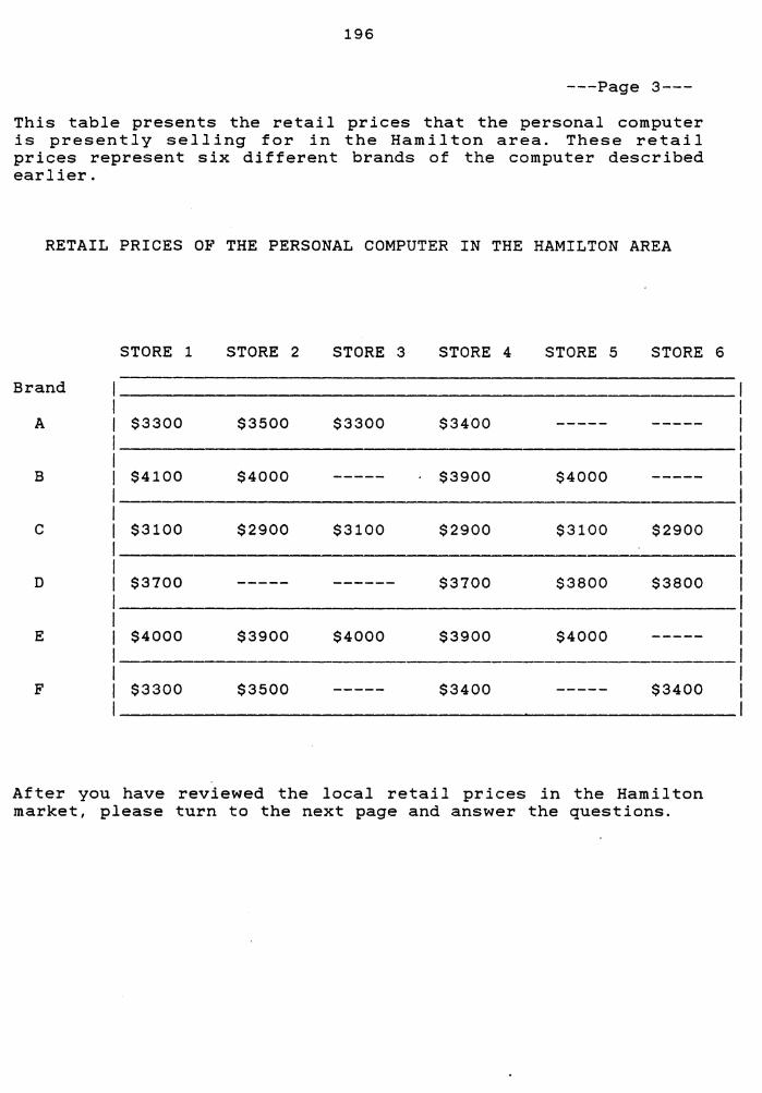
196

---Page 3---

This table presents the retail prices that the personal computer is presently selling for in the Hamilton area. These retail prices represent six different brands of the computer described earlier.

RETAIL PRICES OF THE PERSONAL COMPUTER IN THE HAMILTON AREA

STORE 1 STORE 2 STORE 3 STORE 4 STORE 5 STORE

Brand

A $3300 $3500 $3300 $3400 ----- -----

B $4100 $4000 ----- $3900 $4000 -----

c $3100 $2900 $3100 $2900 $3100 $2900

D $3700 ----- ------ $3700 $3800 $3800

E $4000 $3900 $4000 $3900 $4000 -----

F $3300 $3500 ----- $3400 ----- $3400

After you have reviewed the local retail prices in the Hamilton market, please turn to the next page and answer the questions.

6

197

---Page 4---

Please answer the following questions based on the retail prices for the personal computer provided above.

1. What is the highest retail price offered in Hamilton?

2. What is the lowest retail price offered in Hamilton?

3. Give the number of different prices offered in Hamilton.

4. What is your estimate of the average retail price in Hamilton?

After you have completed this task please turn to the next page and read the instructions.

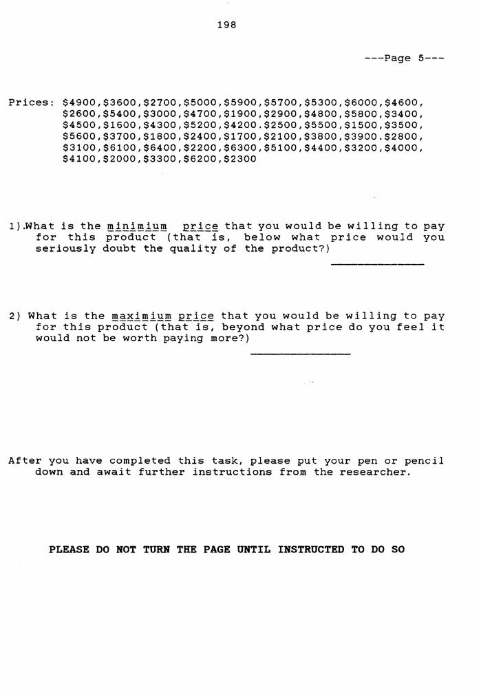
198

---Page 5---

Prices: $4900,$3600,$2700,$5000,$5900,$5700,$5300,$6000,$4600, $2600,$5400,$3000,$4700,$1900,$2900,$4800,$5800,$3400, $4500,$1600,$4300,$5200,$4200.$2500,$5500,$1500,$3500, $5600,$3700,$1800,$2400,$1700,$2100,$3800,$3900.$2800, $3100,$6100,$6400,$2200,$6300,$5100,$4400,$3200,$4000, $4100,$2000,$3300,$6200,$2300

1).What is the m!n!m!Yfil 12.!:i.£~ that you would be willing to pay for this product (that is, below what price would you seriously doubt the quality of the product?)

2) What is the fil~~!m!Yfil 12.!:i.£~ that you would be willing to pay for this product (that is, beyond what price do you feel it would not be worth paying more?)

After you have completed this task, please put your pen or pencil down and await further instructions from the researcher.

PLEASE DO NOT TURN THE PAGE UNTIL INSTRUCTED TO DO SO

199

---Page 6---PLEASE ANSWER THE FOLLOWING QUESTIONS.

1. Have you shopped for a personal computer in the past six months?

YES

[ ] NO

2. Have you purchased a personal computer in the past six months?

YES (continue with question 3)

[ NO (go to question 6)

3. As best as you can recall, how many different brands or models did you examine?

4. How important was price in your initial purchase decision?

VERY IMPORTANT

[ ] SOMEWHAT IMPORTANT

[ SOMEWHAT UNIMPORTANT

] NOT IMPORTANT

5. How important was price in your final purchase decision?

VERY IMPORTANT

[ ] SOMEWHAT IMPORTANT

[ ] SOMEWHAT UNIMPORTANT

] NOT IMPORTANT

6. In the preceding task, did you consider any of the prices as unacceptable?

] YES (continue with question 7)

[ NO (go to question 8)

200

---Page 7---

7. Why were those prices unacceptable? ( List as many reasons as you wish).

8. How knowledgeable would you say you are about the prices of personal computers?

[ ] VERY KNOWLEDGEABLE

] SOMEWHAT KNOWLEDGEABLE

] SOMEWHAT UNKNOWLEDGEABLE

[ ] NOT KNOWLEDGEABLE

9. What do you think the investigator is interested in determining from this study?

AFTER COMPLETING THIS BOOKLET, PLEASE PLACE THE BOOKLET IN THE ENVELOPE AND RAISE YOUR HAND TO INDICATE THAT YOU HAVE COMPLETED THIS PART OF THE RESEARCH STUDY.

THANK YOU FOR YOUR COOPERATION.

a XION:3:ddV

202

STUDENT NAME

STUDENT NUMBER ~~~~~~~~~~~~~

RESPONSE BOOKLET 02

203

---Page 1---

INSTRUCTIONS

On your desk should be an instruction booklet and an envelope. When the researcher tells you to begin, turn to page 2 of the instruction booklet. There you will find a product description and price information. Assume you are interested in buying that product and read the description.

After you have read the product description and the price information, empty the envelope and note its contents. These "PRICE CARDS" represent different price offerings for the product. The objective is to sort out the prices into a number of piles you choose. Decide on the piles on the basis of which prices (CARDS) seem to belong together. You may use as many piles as you wish. Do not be concerned about how many piles you create. If you change your mind about any of the prices you have placed in any of the piles, please feel free to rearrange the prices.

After you have finished placing the prices in as many or as few piles as you like, put your pen or pencil down and look up to indicate that you have completed the task. Do NOT turn the page of your instruction booklet.

Are these instructions clear? If not, raise your hand.

In a moment we will begin. Remember, you must:

(1) turn to page 2 of the instruction booklet and read the product description and price information.

(2) empty the contents of the envelope and sort the price cards into as many or as few piles as you choose.

PLEASE DO NOT TURN THE PAGE UNTIL INSTRUCTED TO DO SO

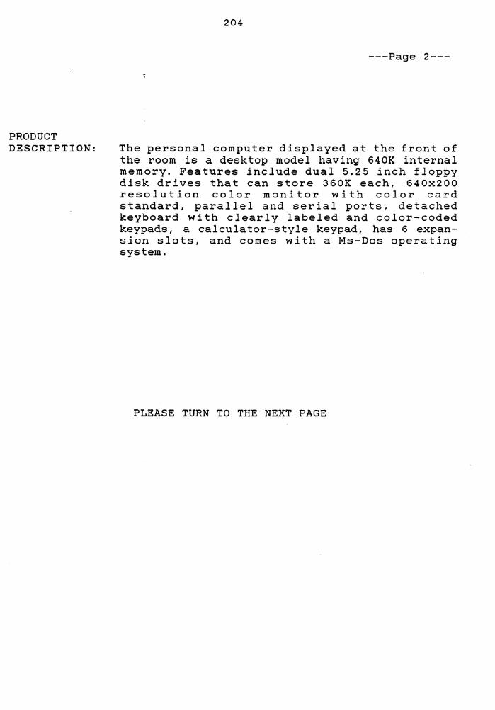
PRODUCT DESCRIPTION:

204

---Page 2---

The personal computer displayed at the front of the room is a desktop model having 640K internal memory. Features include dual 5.25 inch floppy disk drives that can store 360K each, 640x200 resolution color monitor with color card standard, parallel and serial ports, detached keyboard with clearly labeled and color-coded keypads, a calculator-style keypad, has 6 expan-sion slots, and comes with a Ms-Dos operating system.

PLEASE TURN TO THE NEXT PAGE

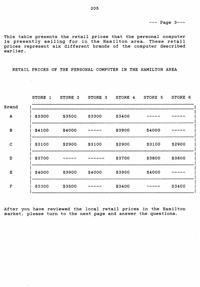
205

--- Page 3---

This table presents the retail prices that the personal computer is presently selling for in the Hamilton area. These retail prices represent six different brands of the computer described earlier.

RETAIL PRICES OF THE PERSONAL COMPUTER IN THE HAMILTON AREA

STORE 1 STORE 2 STORE 3 STORE 4 STORE 5 STORE 6

Brand

A $3300 $3500 $3300 $3400 ----- -----

B $4100 $4000 ----- $3900 $4000 -----

c $3100 $2900 $3100 $2900 $3100 $2900

D $3700 ----- ------ $3700 $3800 $3800

E $4000 $3900 $4000 $3900 $4000 -----

F $3300 $3500 ----- $3400 ----- $3400

After you have reviewed the local retail prices in the Hamilton market, please turn to the next page and answer the questions.

206

---Page 4---

Please answer the following questions based on the retail prices for the personal computer provided above.

1. What is the highest retail price offered in Hamilton?

2. What is the lowest retail price offered in Hamilton?

3. Give the number of different prices offered in Hamilton.

4. What is your estimate of the average retail price in Hamilton?

After you have completed this task please turn to the next page and read the instructions.

207

---Page 5---

INSTRUCTIONS --- 2

On the desk in front of you should be the price cards in the pile or piles that you have created. If the pile or piles of price cards contain prices that are ACCEPTABLE to you (that you would be willing to pay for this product), you are requested to put the pile or piles of prices on the left side of the desk. When this is completed, if there is a pile or piles of prices that are UNACCEPTABLE to you put them on the right side of your desk. Lastly, put any pile or piles of prices that may be NEITHER ACCEPTABLE NOR UNACCEPTABLE to you ih the center of your desk.

Feel free to rearrange any price cards or piles of prices that you wish.

When this task is completed look straight ahead so the researcher will know you are finished.

Are the instructions clear? If not, raise your hand.

PLEASE DO NOT TURN THE PAGE UNTIL INSTRUCTED TO DO SO

208

---Page 6---

INSTRUCTIONS --- 3

You should now have the price cards arranged on the left, right and/or center of your desk along with a second envelope. Open the envelope and note its contents. Inside the envelope should be some paper clips and two sets of seven "LABEL CARDS" for naming the piles you have created into categories. Read the labels.

Your task is to label the pile or piles of price cards that are on your desk. You may use as many or as few of the labels as you wish but each pile of price cards must have a label. When you have decided which label to use for a particular pile, put that label card on top of the piles of prices that you have selected. Continue until all the piles of price cards have labels. When you have completed this task examine the price cards again to make sure you like where they are. If you don't like where they are you may rearrange any price cards or piles of prices, and relabel the pile.

When all the piles of price cards have label cards on them put a paper clip on each pile. Then put the clipped piles of price cards and any unused label cards back in one of the envelopes.

When this task is completed, please turn the page and answer the questions.

209

---Page 7---

PLEASE ANSWER THE FOLLOWING QUESTIONS.

1. Have you shopped for a personal computer in the past six months?

[ ] YES

[ ] NO

2. Have you purchased a personal computer in the past six months?

[ YES (continue with question 3)

[ ] NO (go to question 6)

3. As best as you can recall, how many different brands or models did you examine?

4. How important was price in your initial purchase decision?

[ ] VERY IMPORTANT

] SOMEWHAT IMPORTANT

[ ] SOMEWHAT UNIMPORTANT

[ ] NOT IMPORTANT

5. How important was price in your final purchase decision?

[ ] VERY IMPO.RTANT

[ ] SOMEWHAT IMPORTANT

[ ] SOMEWHAT UNIMPORTANT

[ ] NOT IMPORTANT

6. In the preceding task, did you consider any of the prices as unacceptable?

[ ] YES (continue with question 7)

[ ] NO (go to question 8)

210

---Page 8--

7. Why were those prices unacceptable? ( List as many reasons as you wish).

8. How knowledgeable would you say you are about the prices of personal computers?

] VERY KNOWLEDGEABLE

[ ] SOMEWHAT KNOWLEDGEABLE

SOMEWHAT UNKNOWLEDGEABLE

[ ] NOT KNOWLEDGEABLE

9. What do you think the investigator is interested in determining from this study?

AFTER COMPLETING THIS BOOKLET, PLEASE PLACE THE BOOKLET IN THE ENVELOPE AND RAISE YOUR HAND TO INDICATE THAT YOU HAVE COMPLETED THIS PART OF THE RESEARCH STUDY.

THANK YOU FOR YOUR COOPERATION.

APPENDIX E

211

212

ACCEPTABLE PRICE FREQUENCY FOR STOETZEL AND OWN-CATEGORY LOWER PRICE LIMIT RESULTS OF INSTRUMENT PRETEST/PHASE 1

FREQUENCY

15 2 4 2 1 2 2 3 1 1 1

14 1 2 1 4 1 2 1 5 1 1 1

STOETZEL METHOD

RELATIVE CUMULATIVE FREQUENCY FREQUENCY

44.1 44.1 5.9 50.0

11. 8 61. 8 5.9 67.6 2.9 70.6 5.9 76.5 5.9 82.4 8.8 91. 2 2.9 94.1 2.9 97.1 2.9 100.0

OWN-CATEGORY METHOD

41. 2 41. 2 2.9 44.1 5.9 50.0 2.9 52.9

11. 8 64.7 2.9 67.6 5.9 73.5 2.9 76.5

14.7 91. 2 2.9 94.1 2.9 97.1 2.9 100.0

LOWER PRICE LIMIT

1500 1700 1800 1900 2000 2100 2200 2800 3000 3500 3800

1500 1600 1700 1800 1900 2000 2100 2500 2600 3000 3400 4100

* Subjects evaluated a range of 50 prices from $1500 to $6400 at intervals of $100. Only those prices that subjects indicated as their lower price limit appear.

213

ACCEPTABLE PRICE FREQUENCY FOR STOETZEL AND OWN-CATEGORY UPPER PRICE LIMIT RESULTS OF INSTRUMENT PRETEST/PHASE 1

STOETZEL METHOD

FREQUENCY RELATIVE CUMULATIVE UPPER PRICE FREQUENCY FREQUENCY LIMIT

1 2.9 2.9 2000 2 5.9 a.a 2100 4 11. 8 20.6 2500 1 2.9 23.5 2600 3 a.8 32.4 3000 1 2.9 35.3 3100 1 2.9 sa.2 3200 3 8.a 47.1 3500 1 2.9 50.0 3600 3 8.8 58.8 3700 1 2.9 61. a 3900 2 5.9 67.6 4000 2 5.9 73.5 4200 1 2.9 76.5 4300 5 14.7 91. 2 4500 1 2.9 94.1 4600 1 2.9 97.1 4700 1 2.9 100.0 6000

OWN-CATEGORY METHOD

1 2.9 2.9 2000 1 2.9 5.9 2100 1 2.9 8.8 2700 2 5.9 14.7 2800 1 2.9 17.6 2900 1 2.9 20.6 3000 1 2.9 23.5 3100 2 5.9 29.4 3200 3 8.8 38.2 3500 2 5.9 44.1 3700 1 2.9 47.1 3800 1 2.9 50.0 3900 3 a.8 58.8 4000 1 2.9 61. a 4200 1 2.9 64.7 4300 2 5.9 70.6 4400 3 8.8 79.4 4500 3 8.8 8a.2 4900 1 2.9 91. 2 5300 1 2.9 94.1 5800 2 5.9 100.0 5900

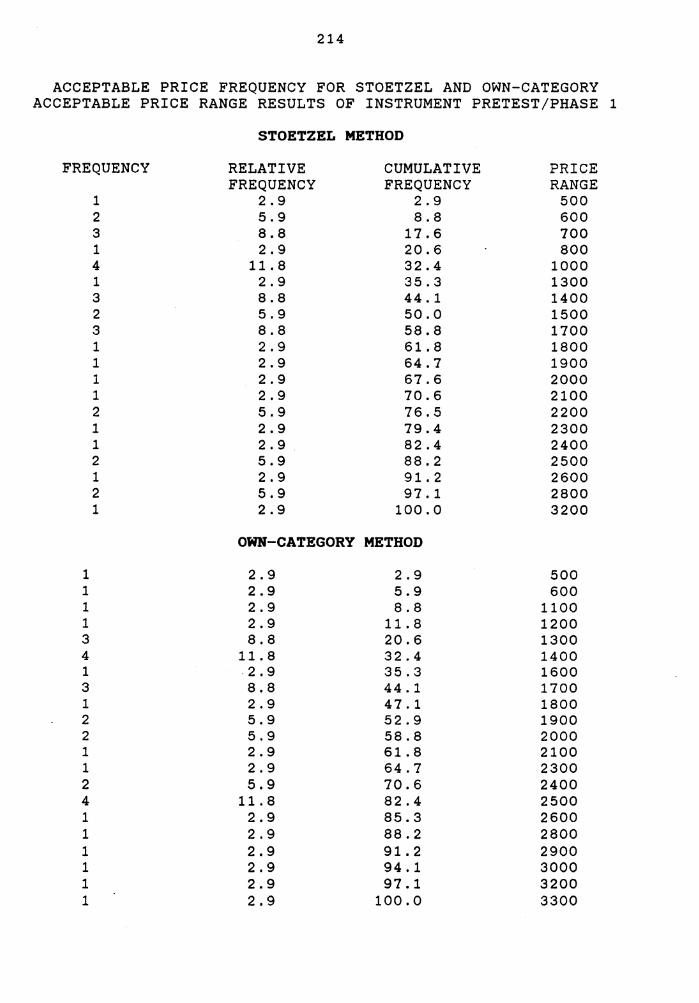
214

ACCEPTABLE PRICE FREQUENCY FOR STOETZEL AND OWN-CATEGORY ACCEPTABLE PRICE RANGE RESULTS OF INSTRUMENT PRETEST/PHASE 1

STOETZEL METHOD

FREQUENCY RELATIVE CUMULATIVE PRICE FREQUENCY FREQUENCY RANGE

1 2.9 2.9 500 2 5.9 8.8 600 3 8.8 17.6 700 1 2.9 20.6 800 4 11. 8 32.4 1000 1 2.9 35.3 1300 3 8.8 44.1 1400 2 5.9 50.0 1500 3 8.8 58.8 1700 1 2.9 61. 8 1800 1 2.9 64.7 1900 1 2.9 67.6 2000 1 2.9 70.6 2100 2 5.9 76.5 2200 1 2.9 79.4 2300 1 2. 9 . 82.4 2400 2 5.9 88.2 2500 1 2.9 91. 2 2600 2 5.9 97.1 2800 1 2.9 100.0 3200

OWN-CATEGORY METHOD

1 2.9 2.9 500 1 2.9 5.9 600 1 2.9 8.8 1100 1 2.9 11. 8 1200 3 8.8 20.6 1300 4 11. 8 32.4 1400 1 .2.9 35.3 1600 3 8.8 44.1 1700 1 2.9 47.1 1800 2 5.9 52.9 1900 2 5.9 58.8 2000 1 2.9 61.8 2100 1 2.9 64.7 2300 2 5.9 70.6 2400 4 11. 8 82.4 2500 1 2.9 85.3 2600 1 2.9 88.2 2800 1 2.9 91. 2 2900 1 2.9 94.1 3000 1 2.9 97.1 3200 1 2.9 100.0 3300

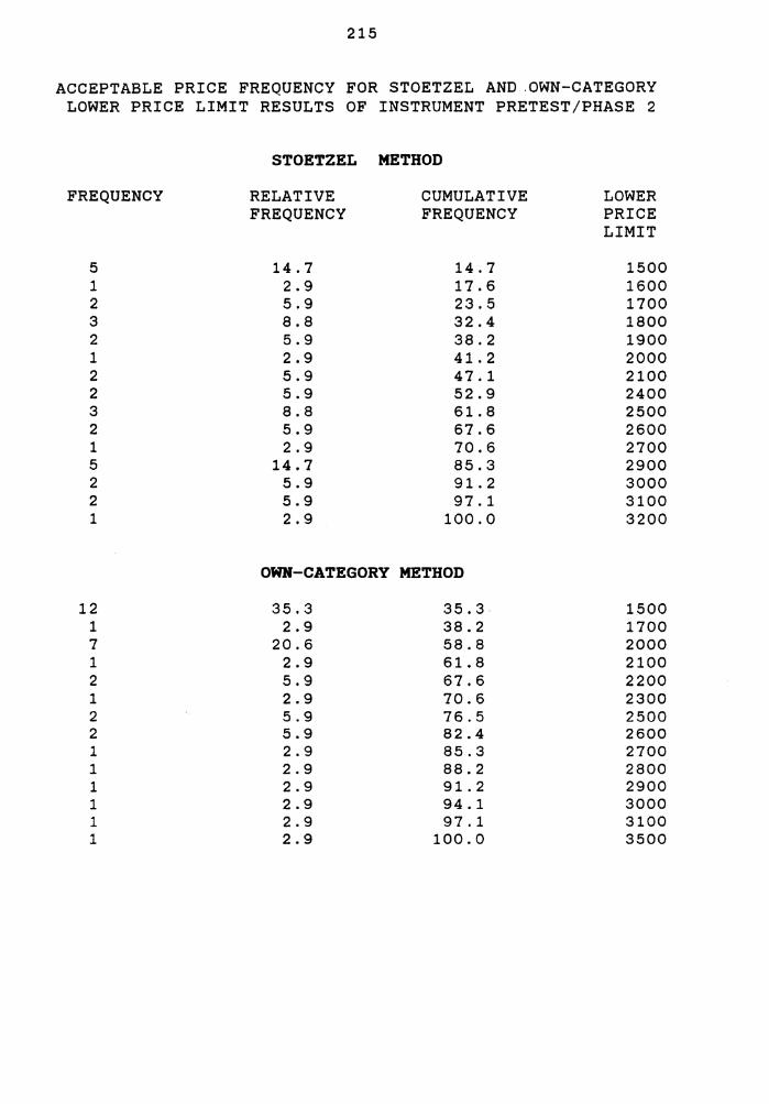
215

ACCEPTABLE PRICE FREQUENCY FOR STOETZEL AND .OWN-CATEGORY LOWER PRICE LIMIT RESULTS OF INSTRUMENT PRETEST/PHASE 2

FREQUENCY

5 1 2 3 2 1 2 2 3 2 1 5 2 2 1

12 1 7 1 2 1 2 2 1 1 1 1 1 1

STOETZEL METHOD

RELATIVE CUMULATIVE FREQUENCY FREQUENCY

14.7 14.7 2.9 17.6 5.9 23.5 8.8 32.4 5.9 38.2 2.9 41. 2 5.9 47.1 5.9 52.9 8.8 61. 8 5.9 67.6 2.9 70.6

14.7 85.3 5.9 91. 2 5.9 97.1 2.9 100.0

OWN-CATEGORY METHOD

35.3 35.3. 2.9 38.2

20.6 58.8 2.9 61. 8 5.9 67.6 2.9 70.6 5.9 76.5 5.9 82.4 2.9 85.3 2.9 88.2 2.9 91. 2 2.9 94.1 2.9 97.1 2.9 100.0

LOWER PRICE LIMIT

1500 1600 1700 1800 1900 2000 2100 2400 2500 2600 2700 2900 3000 3100 3200

1500 1700 2000 2100 2200 2300 2500 2600 2700 2800 2900 3000 3100 3500

216

ACCEPTABLE PRICE FREQUENCY FOR STOETZEL AND OWN-CATEGORY UPPER PRICE LIMIT RESULTS OF INSTRUMENT PRETEST/PHASE 2

FREQUENCY

1 1 1 2 2 2 4 1 3 4 1 4 2 2 4

2 1 1 1 6 2 2 6 2 1 1 2 1 4 1 1

STOETZEL METHOD

RELATIVE CUMULATIVE FREQUENCY H'REQUENCY

2.9 2.9 2.9 5.9 2.9 8.8 5.9 14.7 5.9 20.6 5.9 26.5

11. 8 38.2 2.9 41. 2 8.8 50.0

11. 8 61. 8 2.9 64.7

11. 8 76.5 5.9 82.4 5.9 88.2

11. 8 100.0

OWN-CATEGORY METHOD

5.9 5.9 2.9 8.8 2.9 11. 8 2.9 14.7

17.6 32.4 5.9 38.2 5.9 44.1

17.6 61. 8 5.9 67.6 2.9 70.6 2.9 73.5 5.9 79.4 2.9 82.4

11. 8 94.1 2.9 97.1 2.9 100.0

UPPER PRICE LIMIT

2700 2900 3000 3200 3300 3400 3500 3600 3700 3800 3900 4000 4100 4200 4500

2900 3000 3100 3400 3500 3700 3800 3900 4000 4100 4300 4600 4700 4900 5200 5500

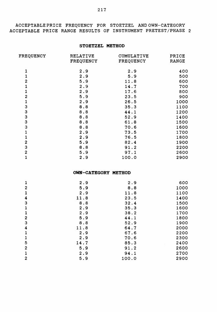
217

ACCEPTABLE PRICE FREQUENCY FOR STOETZEL AND OWN-CATEGORY ACCEPTABLE PRICE RANGE RESULTS OF INSTRUMENT PRETEST/PHASE 2

STOETZEL METHOD

FREQUENCY RELATIVE CUMULATIVE PRICE FREQUENCY FREQUENCY RANGE

1 2.9 2.9 400 1 2.9 5.9 500 2 5.9 11. 8 600 1 2.9 14.7 700 1 2.9 17.6 800 2 5.9 23.5 900 1 2.9 26.5 1000 3 8.8 35.3 1100 3 8.8 44.1 1200 3 8.8 52.9 1400 3 8.8 61. 8 1500 3 8.8 70.6 1600 1 2.9 73.5 1700 1 2.9 76.5 1800 2 5.9 82.4 1900 3 8.8 91. 2 2200 2 5.9 97.1 2600 1 2.9 100.0 2900

OWN-CATEGORY METHOD

1 2.9 2.9 600 2 5.9 8.8 1000 1 2.9 11. 8 1100 4 11. 8 23.5 1400 3 8.8 32.4 1500 1 2.9 35.3 1600 1 2.9 38.2 1700 2 5.9 44.1 1800 3 8.8 52.9 1900 4 11.8 64.7 2000 1 2.9 67.6 2200 1 2.9 70.6 2300 5 14.7 85.3 2400 2 5.9 91. 2 2600 1 2.9 94.1 2700 2 5.9 100.0 2900

APPENDIX F

218

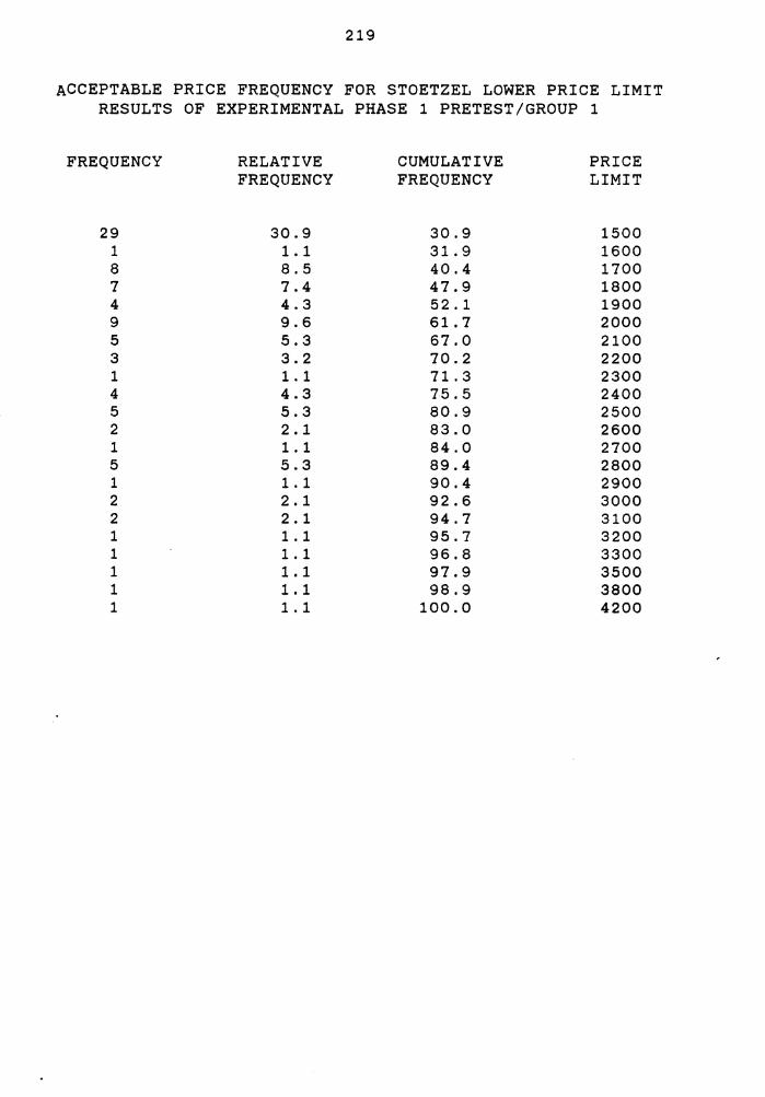
219

ACCEPTABLE PRICE FREQUENCY FOR STOETZEL LOWER PRICE LIMIT RESULTS OF EXPERIMENTAL PHASE 1 PRETEST/GROUP 1

FREQUENCY

29 1 8 7 4 9 5 3 1 4 5 2 1 5 1 2 2 1 1 1 1 1

RELATIVE FREQUENCY

30.9 1.1 8.5 7.4 4.3 9.6 5.3 3.2 1.1 4.3 5.3 2.1 1. 1 5.3 1.1 2. 1 2. 1 1.1 1. 1 1.1 1.1 1.1

CUMULATIVE PRICE FREQUENCY LIMIT

30.9 1500 31. 9 1600 40.4 1700 47.9 1800 52.1 1900 61. 7 2000 67.0 2100 70.2 2200 71.3 2300 75.5 2400 80.9 2500 83.0 2600 84.0 2700 89.4 2800 90.4 2900 92.6 3000 94.7 3100 95.7 3200 96.8 3300 97.9 3500 98.9 3800

100.0 4200

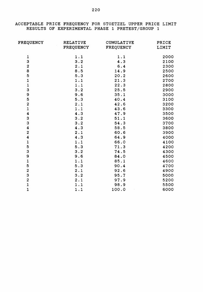
220

ACCEPTABLE PRICE FREQUENCY FOR STOETZEL UPPER PRICE LIMIT RESULTS OF EXPERIMENTAL PHASE 1 PRETEST/GROUP 1

FREQUENCY RELATIVE CUMULATIVE PRICE FREQUENCY FREQUENCY LIMIT

1 1.1 1.1 2000 3 3.2 4.3 2100 2 2.1 6.4 2300 8 8.5 14.9 2500 5 5.3 20.2 2600 1 1.1 21. 3 2700 1 1.1 22.3 2800 3 3.2 25.5 2900 9 9.6 35.1 3000 5 5.3 40.4 3100 2 2. 1 42.6 3200 1 1.1 43.6 3300 4 4.3 47.9 3500 3 3.2 51.1 3600 3 3.2 54.3 3700 4 4.3 58.5 3800 2 2. 1 60.6 3900 4 4.3 64.9 4000 1 1.1 66.0 4100 5 5.3 71. 3 4200 3 3.2 74.5 4300 9 9.6 84.0 4500 1 1.1 85.1 4600 5 5.3 90.4 4700 2 2. 1 92.6 4900 3 3.2 95.7 5000 2 2. 1 97.9 5200 1 1.1 98.9 5500 1 1.1 100.0 6000

221

ACCEPTABLE PRICE FREQUENCY FOR STOETZEL PRICE RANGE RESULTS OF EXPERIMENTAL PHASE 1 PRETEST/GROUP 1

FREQUENCY RELATIVE CUMULATIVE PRICE FREQUENCY FREQUENCY RANGE

1 1.1 1.1 400 2 2. 1 3.2 500 4 4.3 7.4 600 6 6.4 13.8 700 3 3.2 17.0 800 2 2. 1 19.1 900

10 10.6 29.8 1000 5 5.3 35.1 1100 6 6.4 41. 5 1200 3 3.2 44.7 1300 4 4.3 48.9 1400 5 5.3 54.3 1500 5 5.3 59.6 1600 4 4.3 63.8 1700 2 2. 1 66.0 1800 3 3.2 69.1 1900 5 5.3 74.5 2000 3 3.2 77.7 2100 3 3.2 80.9 2200 3 3.2 84.0 2300 2 2.1 86.2 2400 5 5.3 91. 5 2500 2 2.1 93.6 2600 2 2.1 95.7 2800 2 2.1 97.9 3000 1 1.1 98.9 3200 1 1.1 100.0 4000

222

ACCEPTABLEPRICEFREQUENCY FOR OWN-CATEGORYLOWERPRICE LIMIT RESULTS OF EXPERIMENTAL PHASE 1 PRETEST/GROUP 1

FREQUENCY RELATIVE CUMULATIVE PRICE FREQUENCY FREQUENCY LIMIT

30 31. 9 31. 9 1500 4 4.3 36.2 1600 4 4.3 40.4 1700 2 2.1 42.6 1800 9 9.6 52.1 1900

10 10.6 62.8 2000 3 3.2 66.0 2100 2 2 .1 68.1 2200 1 1.1 69.1 2300 2 2. 1 71.3 2400 7 7.4 78.7 2500 8 8.5 87.2 2600 2 2.1 89.4 2900 4 4.3 93.6 3000 1 1.1 94.7 3100 2 2.1 96.8 3300 1 1.1 97.9 3400 1 1.1 98.9 3500 1 1.1 100.0 4100

223

ACCEPTABLE PRICE FREQUENCY FOR OWN-CATEGORY UPPER PRICE LIMIT RESULTS OF EXPERIMENTAL PHASE 1 PRETEST/GROUP 1

FREQUENCY RELATIVE CUMULATIVE PRICE FREQUENCY FREQUENCY LIMIT

1 1.1 1.1 2000 1 1.1 2.1 2100 2 2. 1 4.3 2600 1 1.1 5.3 2700 3 3.2 8.5 2800 8 8.5 17.0 2900 4 4.3 21. 3 3000 1 1.1 22.3 3100 3 3.2 25.5 3200 1 1.1 26.6 3300 7 7.4 34.0 3400 6 6.4 40.4 3500 2 2. 1 42.6 3600 5 5.3 47.9 3700 1 1.1 48.9 3800 6 6.4 55.3 3900 3 3.2 58.5 4000 2 2. 1 60.6 4200 2 2. 1 62.8 4300 7 7.4 70.2 4400 5 5.3 75.5 4500 2 2.1 77.7 4600 2 2.1 79.8 4700 1 1.1 80.9 4800 9 9.6 90.4 4900 1 1.1 91. 5 5000 1 1.1 92.6 5200 2 2.1 94.7 5300 1 1.1 95.7 5600 1 1.1 96.8 5700 1 1. 1 97.9 5800 2 2.1 100.0 5900

224

ACCEPTABLE PRICE FREQUENCY FOR OWN-CATEGORY PRICE RANGE RESULTS OF EXPERIMENTAL PHASE 1 PRETEST/GROUP 1

FREQUENCY RELATIVE CUMULATIVE PRICE FREQUENCY FREQUENCY PRICE

2 2.1 2. 1 500 1 1.1 3.2 600 1 1.1 4.3 700 2 2. 1 6.4 900 2 2. 1 8.5 1000 2 2.1 10.6 1100 3 3.2 13.8 1200 6 6.4 20.2 1300

14 14.9 35.1 1400 5 5.3 40.4 1500 2 2.1 42.6 1600 4 4.3 46.8 1700 5 5.3 52.1 1800 7 7.4 59.6 1900 6 6.4 66.0 2000 3 3.2 69.1 2100 1 1.1 70.2 2200 2 2. 1 72.3 2300 6 6.4 78.7 2400 5 5.3 84.0 2500 3 3.2 87.2 2600 3 3.2 90.4 2700 1 1.1 91. 5 2800 2 2. 1 93.6 2900 1 1.1 94.7 3000 1 1.1 95.7 3200 1 1.1 96.8 3300 3 3.2 100.0 3400

225

ACCEPTABLE PRICE FREQUENCY FOR STOETZEL LOWER PRICE LIMIT RESULTS OF EXPERIMENTAL PHASE 1 PRETEST/GROUP 2

FREQUENCY

22 5 3 8 6 6 7 4 3 1 2 3 2 2 1

RELATIVE FREQUENCY

29.3 6.7 4.0

10.7 8.0 8.0 9.3 5.3 4.0 1. 3 2.7 4.0 2.7 2.7 1. 3

CUMULATIVE FREQUENCY

29.3 36.0 40.0 50.7 58.7 66.7 76.0 81. 3 85.3 86.7 89.3 93.3 96.0 98.7

100.0

PRICE LIMIT

1500 1600 1700 1800 1900 2000 2100 2200 2500 2600 2700 3000 3100 3500 4000

226

ACCEPTABLE PRICE FREQUENCY FOR STOETZEL UPPER PRICE LIMIT RESULTS OF EXPERIMENTAL PHASE 1 PRETEST/GROUP 2

FREQUENCY RELATIVE CUMULATIVE PRICE FREQUENCY FREQUENCY LIMIT

1 1.3 1.3 1900 2 2.7 4.0 2000 1 1. 3 5.3 2200 1 1. 3 6.7 2300 4 5.3 12.0 2400 7 9.3 21. 3 2500 3 4.0 25.3 2700 1 1. 3 26.7 2900 9 12.0 38.7 3000 1 1. 3 40.0 3100 3 4.0 44.0 3200 1 1. 3 45.3 3400 5 6.7 52.0 3500 3 4.0 56.0 3600 3 4.0 60.0 3700 2 2.7 62.7 3900 9 12.0 74.7 4000 1 1.3 76.0 4100 2 2.7 78.7 4300 3 4.0 82.7 4500 1 1. 3 84.0 4600 2 2.7 86.7 4700 3 4.0 90.7 5000 3 4.0 94.7 5200 1 1. 3 96.0 5500 1 1. 3 97.3 5600 2 2.7 100.0 5800

227

ACCEPTABLE PRICE FREQUENCY FOR STOETZEL PRICE RANGE RESULTS OF EXPERIMENTAL PHASE 1 PRETEST/GROUP 2

FREQUENCY RELATIVE CUMULATIVE PRICE FREQUENCY FREQUENCY RANGE

1 1. 3 1. 3 300 1 1. 3 2.7 400 3 4.0 6.7 500 1 1. 3 8.0 600 1 1. 3 9.3 700 4 5.3 14.7 800 4 5.3 20.0 900 8 10.7 30.7 1000 1 1. 3 32.0 1100 6 8.0 40.0 1200 2 2.7 42.7 1300 2 2.7 45.3 1400 7 9.3 54.7 1500 2 2.7 57.3 1600 3 4.0 61. 3 1700 5 6.7 68.0 1800 1 1. 3 69.3 1900 7 9.3 78.7 2000 2 2.7 81. 3 2200 1 1. 3 82.7 2300 2 2.7 85.3 2400 4 5.3 90.7 2500 1 1. 3 92.0 2600 1 1. 3 93.3 2700 1 1. 3 94.7 2800 1 1. 3 96.0 3000 1 1. 3 97.3 3100 1 1. 3 98.7 3700 1 1. 3 100.0 4100

228

ACCEPTABLE PRICE FREQUENCY FOR OWN-CATEGORY LOWER PRICE LIMIT RESULTS OF EXPERIMENTAL PHASE 1 PRETEST/GROUP 2

FREQUENCY RELATIVE CUMULATIVE PRICE FREQUENCY FREQUENCY LIMIT

1 1. 3 1. 3 1400 28 37.3 38.7 1500

3 4.0 42.7 1700 4 5.3 48.0 1800 5 6.7 54.7 1900 7 9.3 64.0 2000 6 8.0 72.0 2100 7 9.3 81. 3 2200 2 2.7 84.0 2300 1 1. 3 85.3 2400 1 1. 3 86.7 2500 1 1. 3 88.0 2600 3 4.0 92.0 2800 1 1. 3 93.3 3000 2 2.7 96.0 3100 1 1. 3 97.3 3300 1 1. 3 98.7 3500 1 1. 3 100.0 4000

229

ACCEPTABLE PRICE FREQUENCY FOR OWN-CATEGORY UPPER PRICE LIMIT RESULTS OF EXPERIMENTAL PHASE 1 PRETEST/GROUP 2

FREQUENCY RELATIVE CUMULATIVE PRICE FREQUENCY FREQUENCY LIMIT

1 1. 3 1. 3 2100 1 1. 3 2.7 2400 2 2.7 5.3 2500 1 1. 3 6.7 2600 1 1.3 8.0 2700 1 1. 3 9.3 2800 4 5.3 14.7 2900 5 6.7 21. 3 3000 1 1. 3 22.7 3100 5 6.7 29.3 3200 2 2.7 32.0 3300 4 5.3 37.3 3400 4 5.3 42.7 3500 3 4.0 46.7 3600

12 16.0 62.7 3900 7 9.3 72.0 4000 4 5.3 77.3 4300 3 4.0 81. 3 4500 1 1. 3 82.7 4600 4 5.3 88.0 4900 1 1. 3 89.3 5000 2 2.7 92.0 5100 1 1. 3 93.3 5200 3 4.0 97.3 5500 1 1. 3 98.7 5800 1 1. 3 100.0 5900

230

ACCEPTABLE PRICE FREQUENCY FOR OWN-CATEGORY PRICE RANGE RESULTS OF EXPERIMENTAL PHASE 1 PRETEST/GROUP 2

FREQUENCY RELATIVE CUMULATIVE PRICE FREQUENCY FREQUENCY RANGE

1 1. 3 1.3 600 1 1. 3 2.7 700 3 4.0 6.7 800 1 1. 3 8.0 900 3 4.0 12.0 1000 5 6.7 18.7 1100 3 4.0 22.7 1200 3 4.0 26.7 1400 7 9.3 36.0 1500 1 1. 3 37.3 1600 6 8.0 45.3 1700 5 6.7 52.0 1800 8 10.7 62.7 1900 6 8.0 70.7 2000 1 1. 3 72.0 2200 1 1. 3 73.3 2300 7 9.3 82.7 2400 1 1. 3 84.0 2500 2 2.7 86.7 2700 3 4.0 90.7 2800 2 2.7 93.3 2900 3 4.0 97.3 3000 1 1. 3 98.7 3100 1 1. 3 100.0 4000

APPENDIX G

231

232

GROUP MEANS AND STANDARD DEVIATIONS

FOR

STOETZEL PRICE LOWER LIMIT

FULL DATA

Pretest No Pretest

M= 23.513 M= 24.943 Price Information SD= 5.603 SD= 5.809

N= 78 N= 105

M= 19.607 M= 20.000 No Price Information SD= 5.489 SD= 5.838

N= 56 N= 77

Test for Homogeneity of Variance

Cochran's C = 0.26345, p = 1.000*

Bartlett-Box F = 0.11880, p = 0.949

* Approximate

M =Mean Price ( where M = 23.513 equals $2351.30) SD = Standard Deviation (where SD = 5.603 equals $560.30) N = Sample Size

233

GROUP MEANS AND STANDARD DEVIATIONS

FOR

STOETZEL UPPER PRICE LIMIT

FULL DATA

Pretest No Pretest

M= 37.179 M= 37.600 Price Information SD= 4.898 SD= 6.360

N= 78 N= 105

M= 35.964 M= 36.987 No Price Information SD= 9.677 SD= 11.461

N= 56 N= 77

Test for Homogeneity of Variance

Cochran's C = 0.45383, p = .011

Bartlett-Box F = 21.94341, p = .000

234

GROUP MEANS AND STANDARD DEVIATIONS

FOR

STOETZEL PRICE RANGE

FULL DATA

Pretest No Pretest

M= 13.667 M= 12.667 Price Information SD= 6.199 SD= 6.355

N= 78 N= 105

M= 16.357 M= 16.987 No Price Information SD= 8.460 SD= 8.457

N= 56 N= 77

Test of Homogeneity of Variance

Cochran's C = 0.32256, p = 1.000

Bartlett-Box F = 4.51882, p = .004

235

GROUP MEANS AND STANDARD DEVIATIONS

FOR

OWN-CATEGORY LOWER PRICE LIMIT

FULL DATA

Pretest No Pretest

M= 20.780 M= 22.750 Price Information SD= 5.360 SD= 6.454

N= 59 N= 68

M= 19.536 M= 19.271 No Price Information SD= 5.682 SD= 5.332

N= 56 N= 70

Homogeneity of Variance

Cochran's c = 0.31772, p = 1.000

Bartlett-Box F = 1.07279, p = .359

236

GROUP MEANS AND STANDARD DEVIATIONS

FOR

OWN-CATEGORY UPPER PRICE LIMIT

FULL DATA

Pretest No Pretest

M= 39.475 M= 40.044 Price Information SD= 6.149 SD= 8.010

N= 59 N= 68

M= 38.286 M= 38.843 No Price Information SD= 9.049 SD= 10.046

N= 56 N= 77

Test of Homogeneity of Variance

Cochran's C = 0.35439, p = .979

Bartlett-Box F = 5.01241, p = .002

237

GROUP MEANS AND STANDARD DEVIATIONS

FOR

OWN-CATEGORY PRICE RANGE

FULL DATA

Pretest No Pretest

M= 18.695 M= 17.294 Price Information SD= 5.675 SD= 5.823

N= 59 N= 105

M= 18.750 M= 19.571 No Price Information SD= 7.609 SD= 7.788

N= 56 N= 70

Test of Homogeneity of Variance

Cochran's C = 0.32843, p = 1.000

Bartlett-Box= 3.49967, p = .015

238

GROUP MEANS AND STANDARD DEVIATIONS

FOR

STOETZEL LOWER PRICE LIMIT

OUTLIERS DELETED

Pretest No Pretest

M= 23.513 M= 24.943 Price Information SD= 5.603 SD= 5.809

N= 78 N= 105

M= 18.852 M= 20.000 No Price Information SD= 3.749 SD= 5.838

N= 54 N= 77

Test for Homogeneity of Variance

Cochran's C = 0.28860, p = 1.000*

Bartlett-Box F = 2.28061, p = 0.077

* Approximate

239

GROUP MEANS AND STANDARD DEVIATIONS

FOR

STOETZEL UPPER PRICE LIMIT

OUTLIERS DELETED

Pretest No Pretest

M= 36.959 M= 37.711 Price Information SD= 3.988 SD= 4.128

N= 73 N= 90

M= 32.348 M= 31.879 No Price Information SD= 6.056 SD= 7.703

N= 46 N= 58

Test for Homogeneity of Variance

Cochran's C = 0.35434, p = .979

Bartlett-Box F = 12.46387, p'= .000

240

GROUP MEANS AND STANDARD DEVIATIONS

FOR

STOETZEL PRICE RANGE

OUTLIERS DELETED

Pretest No Pretest

M= 13.667 M= 12.625 Price Information SD= 6.199 SD= 6.377

N= 78 N= 104

M= 15.537 M= 16.684 No Price Information SD= 7.417 SD= 8.082

N= 54 N= 76

Test of Homogeneity of Variance

Cochran's C = 0.32782, p = .837

Bartlett-Box F = 2.50428, p = .058

241

GROUP MEANS AND STANDARD DEVIATIONS

FOR

OWN-CATEGORY LOWER PRICE LIMIT

OUTLIERS DELETED

Pretest No Pretest

M= 20.780 M= 22.403 Price Information SD= 5.360 SD= 5.829

N= 59 N= 67

M= 18.566 M= 19.271 No Price Information SD= 3.974 SD= 5.332

N= 53 N= 70

Homogeneity of Variance

Cochran's C = 0.28860, p = 1.000

Bartlett-Box F = 2.50428, p = .058

242

GROUP MEANS AND STANDARD DEVIATIONS

FOR

OWN-CATEGORY UPPER PRICE LIMIT

OUTLIERS DELETED

Pretest No Pretest

M= 38.750 M= 39.687 Price Information SD= 5.408 SD= 7.504

N= 56 N= 67

M= 38.286 M= 38.843 No Price Information SD= 9.049 SD= 10.046

N= 56 N= 70

Test of Homogeneity of Variance

Cochran's C = 0.36444, p = .777

Bartlett-Box F = 5.44969, p = .001

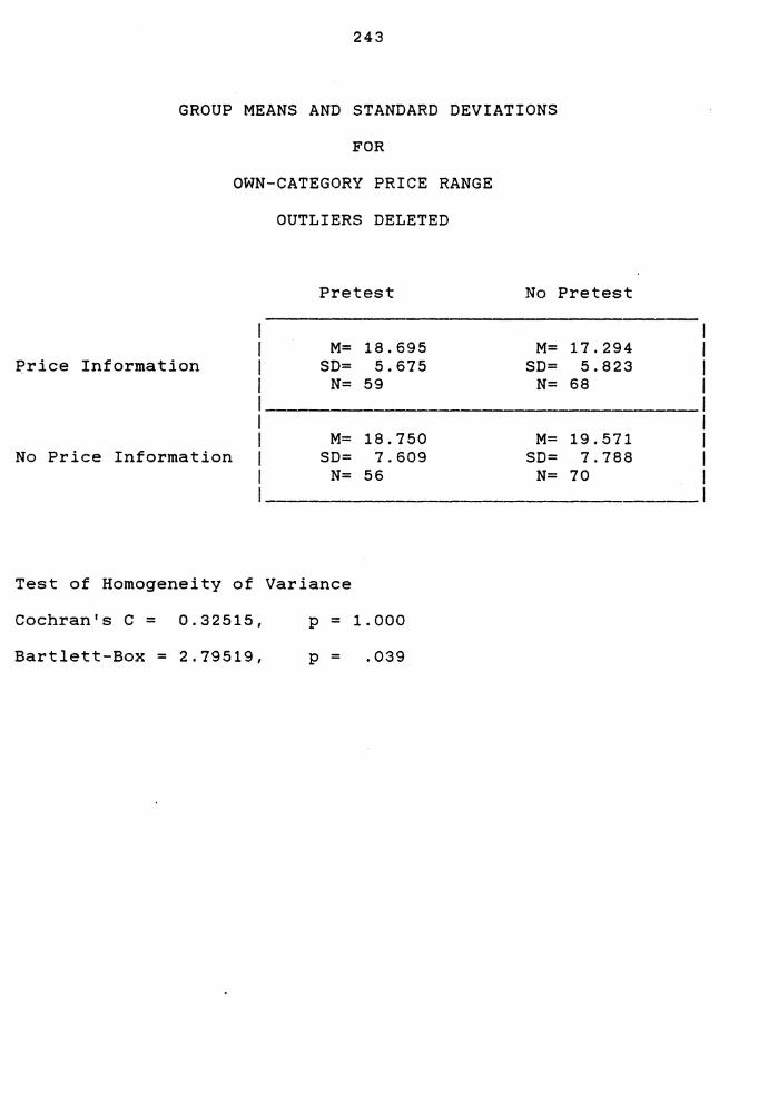
243

GROUP MEANS AND STANDARD DEVIATIONS

FOR

OWN-CATEGORY PRICE RANGE

OUTLIERS DELETED

Pretest No Pretest

M= 18.695 M= 17.294 {>rice Information SD= 5.675 SD= 5.823

N= 59 N= 68

M= 18.750 M= 19.571 No Price Information SD= 7.609 SD= 7.788

N= 56 N= 70

Test of Homogeneity of Variance

Cochran's C = 0.32515, p = 1.000

Bartlett-Box= 2.79519, p = .039

APPENDIX H

244

245

RESULTS OF THREE ANALYSIS OF VARIANCE METHODS FOR UNBALANCED FACTORIAL DESIGNS

SOURCE

MAIN EFFECT

TREATMENT

TEST

INTERACTION

RESIDUAL

TOTAL

SOURCE

MAIN EFFECT

TREATMENT

TEST

INTERACTION

RESIDUAL

TOTAL

FOR THE STOETZEL LOWER PRICE LIMIT USING THE FULL DATA

CLASSICAL REGRESSION EXPERIMENTAL METHOD

METHOD

SUM OF F p SUM OF F SQUARES SQUARES

1635.131 25.071 .000 1517.920 23.273

1562.358 47.910 .001 1472.059 45.141

76.301 2.340 .127 62.475 1. 916

20.225 0.620 .432 20.225 0.620

10174.501 10174.501

11829.858 11829.858

HIERARCHICAL METHOD

SUM OF F p DF SQUARES

1635.131 25.071 .000 2

1558.830 47.801 .000 1

76.301 2.340 .127 1

20.225 0.620 .432 1

10174.501 312

11829.858 315

p

.000

.000

.167

.432

246

RESULTS OF THREE ANALYSIS OF VARIANCE METHODS FOR UNBALANCED FACTORIAL DESIGNS

SOURCE

MAIN EFFECT

TREATMENT

TEST

INTERACTION

RESIDUAL

TOTAL

SOURCE

MAIN EFFECT

TREATMENT

TEST

INTERACTION

RESIDUAL

TOTAL

FOR THE STOETZEL UPPER PRICE LIMIT USING THE FULL DATA

CLASSICAL REGRESSION EXPERIMENTAL

METHOD

SUM OF F p SQUARES

92.533 0.681 .507

58.010 0.854 .356

35.007 0.515 .473

6.818 0.100 .752

21187.603

21286.975

HIERARCHICAL METHOD

SUM OF F SQUARES

92 .553 .681

57.547 .358

35.007 .515

6.818 .100

21187.603

21286.975

METHOD

SUM OF F SQUARES

99.152 o. 730

62.838 0.925

39.162 0.577

6.818 0.100

21187.603

21286.975

p DF

.507 2

.358 1

.473 1

.752 1

312

315

p

.483

.337

.448

.752

247

RESULTS OF THREE ANALYSIS OF VARIANCE METHODS FOR UNBALANCED FACTORIAL DESIGNS

FOR THE STOETZEL PRICE RANGE USING THE FULL DATA

CLASSICAL REGRESSION EXPERIMENTAL METHOD

METHOD

SOURCE SUM OF F p SUM OF F SQUARES SQUARES

MAIN EFFECT 1025.303 9.676 .000 927.172 8.750

TREATMENT 1018.263 19.219 .000 926.615 17.489

TEST 7.943 0 .150 .699 2.710 0.051

INTERACTION 50.530 0.954 .330 50.530 0.954

RESIDUAL 16530.835 16530.835

TOTAL 17606.668 17606.668

HIERARCHICAL METHOD

SOURCE SUM OF F p DF SQUARES

MAIN EFFECT 1025.303 8.676 .000 2

TREATMENT 1017.360 19.201 .000 1

TEST 7.943 0.150 .699 1

INTERACTION 50.530 0.954 .330 1

RESIDUAL 16530.835 312

TOTAL 17606.668 315

p

.000

.000

.821

.330

248

RESULTS OF THREE ANALYSIS OF VARIANCE METHODS FOR UNBALANCED FACTORIAL DESIGNS

SOURCE

MAIN EFFECT

TREATMENT

TEST

INTERACTION

RESIDUAL

TOTAL

SOURCE

MAIN EFFECT

TREATMENT

TEST

INTERACTION

RESIDUAL

TOTAL

FOR THE OWN-CATEGORY LOWER PRICE LIMIT USING THE FULL DATA

CLASSICAL REGRESSION EXPERIMENTAL METHOD

METHOD

SUM OF F p SUM OF F SQUARES SQUARES

424.882 6.455 .002 390.109 5.927

383.564 11.655 .001 349.575 10.622

46.544 1. 414 .235 45.622 1.386

78.271 2.378 .124 78.271 2.371

8194.657 8194.657

8697.810 8697.810

HIERARCHICAL METHOD

SUM OF F p DF SQUARES

424.882 6.455 .002 2

378.338 11. 496 .001 1

46.544 1.4141 .235 1

78.271 2.378 .124 1

8194.657 312

8697.810 315

p

.003

.001

.240

.124

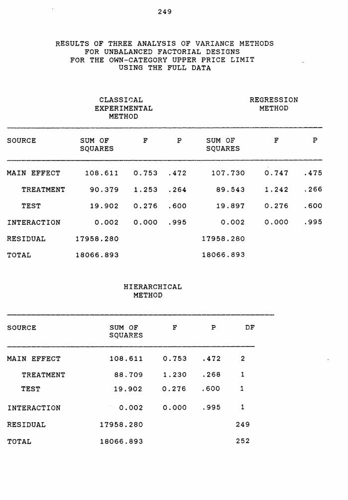
249

RESULTS OF THREE ANALYSIS OF VARIANCE METHODS FOR UNBALANCED FACTORIAL DESIGNS

SOURCE

MAIN EFFECT

TREATMENT

TEST

INTERACTION

RESIDUAL

TOTAL

SOURCE

MAIN EFFECT

TREATMENT

TEST

INTERACTION

RESIDUAL

TOTAL

FOR THE OWN-CATEGORY UPPER PRICE LIMIT USING THE FULL DATA

CLASSICAL REGRESSION EXPERIMENTAL

METHOD

SUM OF F p SQUARES

108.611 0.753 .472

90.379 1.253 .264

19.902 0.276 .600

0.002 0.000 .995

17958.280

18066.893

HIERARCHICAL METHOD

SUM OF F SQUARES

108.611 0.753

88.709 1.230

19.902 0.276

0.002 0.000

17958.280

18066.893

METHOD

SUM OF F SQUARES

107.730 0.747

89.543 1.242

19.897 0.276

0.002 0.000

17958.280

18066.893

p DF

.472 2

.268 1

.600 1

.995 1

249

252

p

.475

.266

.600

.995

250

RESULTS OF THREE ANALYSIS OF VARIANCE METHODS FOR UNBALANCED FACTORIAL DESIGNS

SOURCE

MAIN EFFECT

TREATMENT

TEST

INTERACTION

RESIDUAL

TOTAL

SOURCE

MAIN EFFECT

TREATMENT

TEST

INTERACTION

RESIDUAL

TOTAL

FOR THE OWN-CATEGORY PRICE RANGE USING THE FULL DATA

CLASSICAL EXPERIMENTAL

METHOD

SUM OF F p SQUARES

106.223 1.149 .319

101.566 2.197 .140

5.575 0.121 .729

77.405 1.674 .197

11510.269

11693.897

HIERARCHICAL METHOD

SUM OF F SQUARES

106.223 1.149

100.648 2.177

5.575 0.121

77.405 1. 674

11510.269

11693.897

REGRESSION METHOD

SUM OF F SQUARES

89.689 0.970

85.270 1.845

5.261 0.114

77.405 1.674

11510.269

11693.897

p DF

.319 2

.141 1

.729 1

.197 1

249

252

p

.380

.176

.736

.197

251

RESULTS OF THREE ANALYSIS OF VARIANCE METHODS FOR UNBALANCED FACTORIAL DESIGNS

SOURCE

MAIN EFFECT

TREATMENT

TEST

INTERACTION

RESIDUAL

TOTAL

SOURCE

MAIN EFFECT

TREATMENT

TEST

INTERACTION

RESIDUAL

TOTAL

FOR THE STOETZEL LOWER PRICE LIMIT USING DATA WITH OUTLIERS DELETED

CLASSICAL EXPERIMENTAL

METHOD

SUM OF F p SQUARES

2107.068 37.197 .000

2044.106 72.172 .000

60.509 2.136 .145

42.869 1.514 .220

8468.498

10618.436

HIERARCHICAL METHOD

SUM OF F SQUARES

2107.068 37.197

2046.559 72.259

60.509 2.136

42.869 1. 514

8468.498

10618.436

REGR'.ESSION METHOD

SUM OF F SQUARES

1958.444 34.574

1929.599 68.129

40.480 1. 429

42.869 1.514

8468.498

10618.436

p DF

.000 2

.000 1

.145 1

.220 1

299

302

p

.000

.000

.233

.220

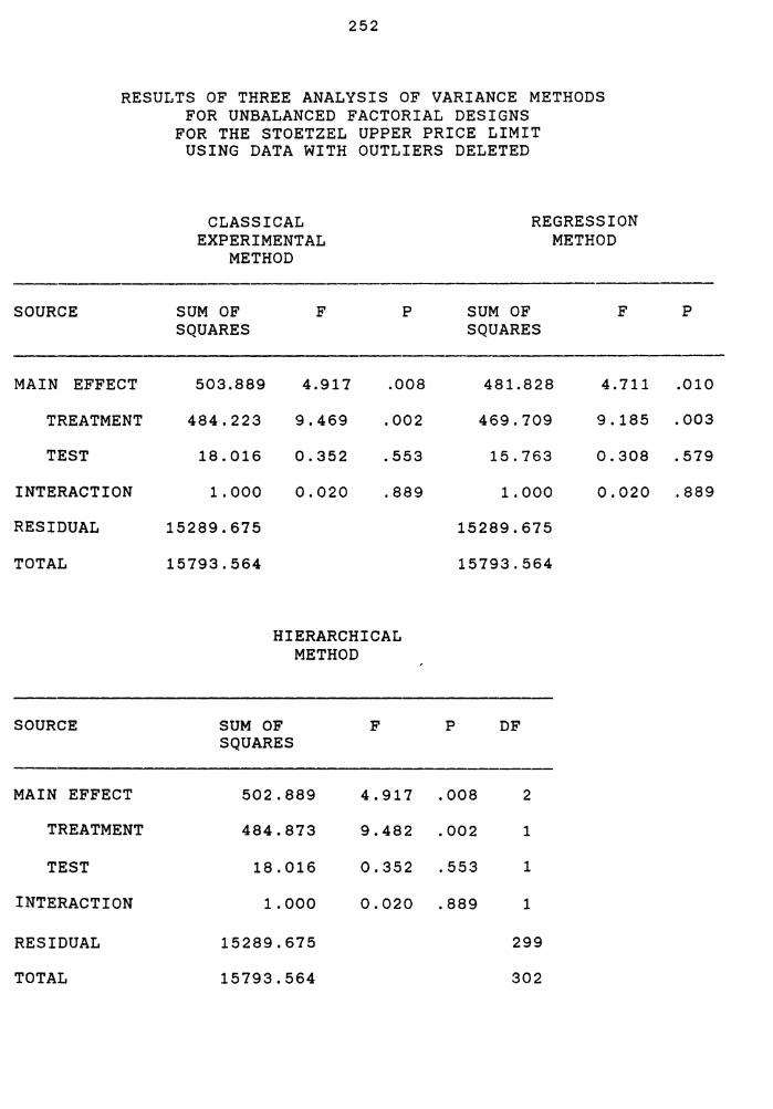
252

RESULTS OF THREE ANALYSIS OF VARIANCE METHODS FOR UNBALANCED FACTORIAL DESIGNS

SOURCE

MAIN EFFECT

TREATMENT

TEST

INTERACTION

RESIDUAL

TOTAL

SOURCE

MAIN EFFECT

TREATMENT

TEST

INTERACTION

RESIDUAL

TOTAL

FOR THE STOETZEL UPPER PRICE LIMIT USING DATA WITH OUTLIERS DELETED

CLASSICAL EXPERIMENTAL

METHOD

SUM OF F p SQUARES

503.889 4.917 .008

484.223 9.469 .002

18.016 0.352 .553

1.000 0.020 .889

15289.675

15793.564

HIERARCHICAL METHOD

SUM OF F SQUARES

502.889 4.917

484.873 9.482

18.016 0.352

1.000 0.020

15289.675

15793.564

REGRESSION METHOD

SUM OF F SQUARES

481.828 4. 711

469.709 9.185

15.763 0.308

1.000 0.020

15289.675

15793.564

p DF

.008 2

.002 1

.553 1

.889 1

299

302

p

.010

.003

.579

.889

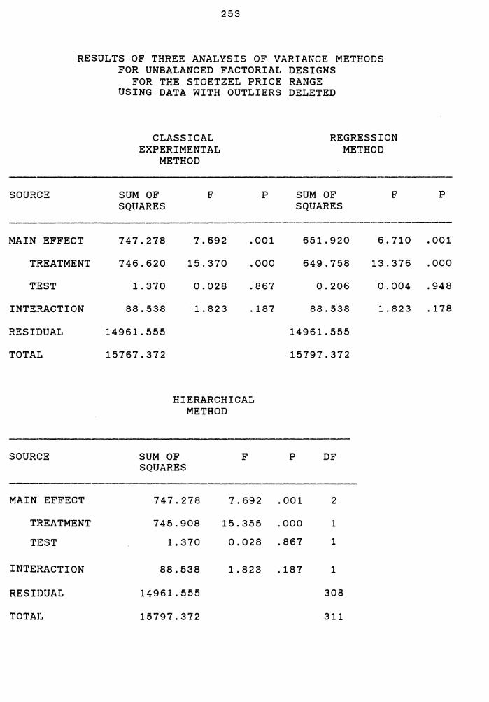
253

RESULTS OF THREE ANALYSIS OF VARIANCE METHODS FOR UNBALANCED FACTORIAL DESIGNS

SOURCE

MAIN EFFECT

TREATMENT

T:E:ST

INTERACTION

RESIDUAL

TOTA:L

SOURCE

MAIN EFFECT

THEATMENT

TgST

INTEHACTION

RESIDUAL

TOTAL

FOR THE STOETZEL PRICE RANGE USING DATA WITH OUTLIERS DELETED

CLASSICAL EXPERIMENTAL

METHOD

SUM OF F p SQUARES

747.278 7.692 .001

746.620 15.370 .000

1.370 0.028 .867

88.538 1.823 .187

14961.555

15767.372

HIERARCHICAL METHOD

SUM OF F SQUARES

747.278 7.692

745.908 15.355

1. 370 0.028

88.538 1. 823

14961.555

15797.372

REGRESSION METHOD

SUM OF F SQUARES

651.920 6.710

649.758 13.376

0.206 0.004

88.538 1.823

14961.555

15797.372

p DF

.001 2

.000 1

.867 1

.187 1

308

311

p

.001

.000

.948

.178

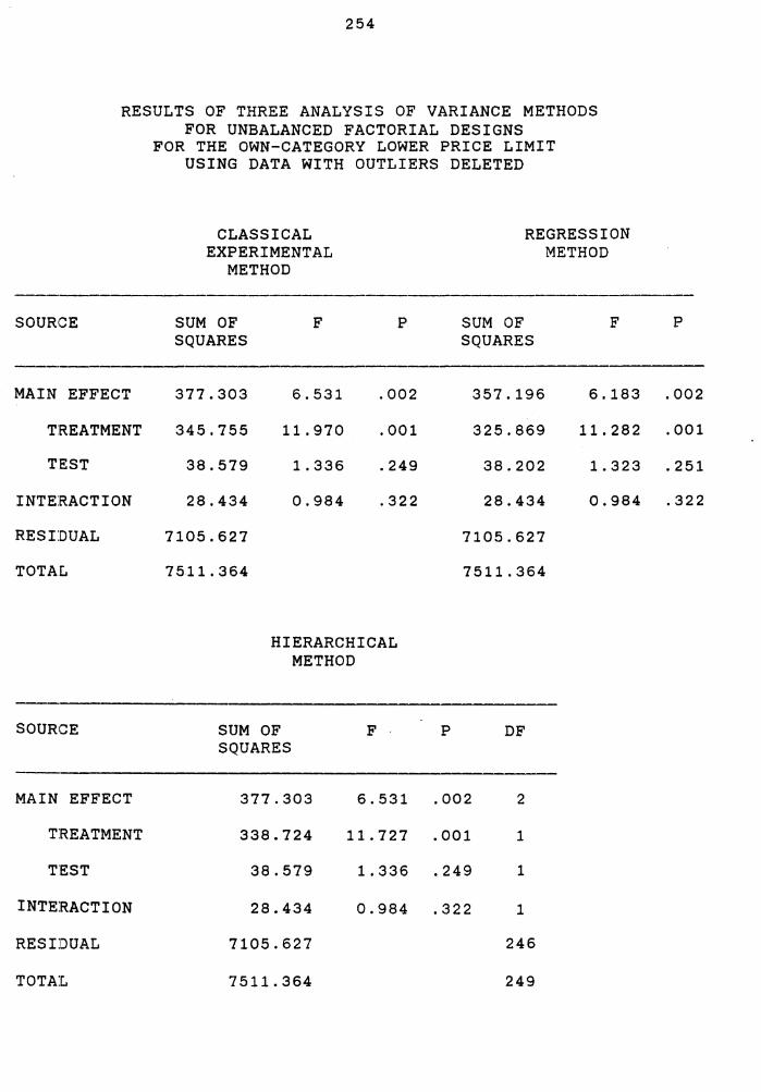
254

RESULTS OF THREE ANALYSIS OF VARIANCE METHODS FOR UNBALANCED FACTORIAL DESIGNS

SO URGE

MAIN EFFECT

TREATMENT

TE:ST

INTERACTION

RESIDUAL

TOTAL

SOURCE

MAIN EFFECT

T:REATMENT

TEST

INTERACTION

RESIDUAL

TO TAI ..

FOR THE OWN-CATEGORY LOWER PRICE LIMIT USING DATA WITH OUTLIERS DELETED

CLASSICAL EXPERIMENTAL

METHOD

SUM OF F p SQUARES

377.303 6.531 .002

345.755 11. 970 .001

38.579 1.336 .249

28.434 0.984 .322

7105.627

7511.364

HIERARCHICAL METHOD

SUM OF F SQUARES

377.303 6.531

338.724 11.727

38.579 1.336

28.434 0.984

7105.627

7511.364

REGRESSION METHOD

SUM OF F SQUARES

357.196 6.183

325.869 11.282

38.202 1.323

28.434 0.984

7105.627

7511.364

p DF

.002 2

.001 1

.249 1

.322 1

246

249

p

.002

.001

.251

.322

255

RESULTS OF THREE ANALYSIS OF VARIANCE METHODS FOR UNBALANCED FACTORIAL DESIGNS

SOURCE

MAIN EFFECT

TREATMENT

T:EST

INTE:~ACTION

RESIDUAL

TOTA:C,

SOURCE

MAIN EFFECT

THEATMENT

TEST

INTEHACTION

RESIDUAL

TOT AI,

FOR THE OWN-CATEGORY UPPER PRICE LIMIT USING DATA WITH OUTLIERS DELETED

CLASSICAL REGRESSION EXPERIMENTAL METHOD

METHOD

SUM OE' E' p SUM OE' E' SQUARES SQUARES

63.554 0.460 .632 67.329 2.487

56.990 0.825 .365 60.730 0.879

7.858 0.114 .736 7.957 0.115

9.596 0.139 .710 9.596 0 .139

16988.786 16988.786

17061.936 17061.936

HIERARCHICAL METHOD

SUM OF F p DF SQUARES

63.554 0.460 .632 2

55.696 0.806 .370 1

7.858 0.114 .736 1

9.596 0.139 .710 1

16988.786 246

17061.936 249

p

.617

.349

.735

.710

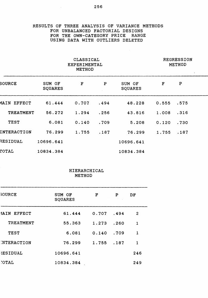
256

RESULTS OF THREE ANALYSIS OF VARIANCE METHODS FOR UNBALANCED FACTORIAL DESIGNS

SOURCE

llJAIN EFFECT

TREATMENT

TEST

INTERACTION

~ESIDUAL

roTAL

30URCE

!AIN E:e'FECT

TREATMENT

TES'r

:NTERAGTION

tESIDUAL

~OTAL

FOR THE OWN-CATEGORY PRICE RANGE USING DATA WITH OUTLIERS DELETED

SUM OF SQUARES

61.444

56.272

6.081

76.299

10696.641

10834.384

CLASSICAL EXPERIMENTAL

METHOD

F p

0.707 .494

1.294 .256

0.140 .709

1.755 .187

HIERARCHICAL METHOD

SUM OF F SQUARES

61.444 0.707

55.363 1.273

6.081 0.140

76.299 1.755

10696.641

10834.384

SUM OF SQUARES

48.228

43.816

5.208

76.299

10696.641

10834.384

p DF

.494 2

.260 1

.709 1

.187 1

246

249

REGRESSION METHOD

F p

0.555 .575

1.008 .316

0.120 .730

1.755 .187

APPENDIX I

257

258

COVARIANCE ANALYSIS RESULTS FOR THE STOETZEL LOWER PRICE LIMIT

CONTROLLING FOR SUBJECT PRICE KNOWLEDGE AND SEX

SUM OF MEAN SOURCE OF VARIATION SQUARES DF SQUARE F

COVA:RIATES 21.649 2 10.825 .391 SEX .553 1 .553 .020 PRICE KNOWLEDGE 17.912 1 17.912 .647

MEAN EFFECTS 1872.536 2 936.268 33.840 TRE:ATMENT 1832.240 1 1832.240 66.224 TESTING EFFECT 68.879 1 68.879 2 .490

2-WAY INTERACTIONS 5.845 1 5.845 .211 TR:E:ATMENT*TEST 5.845 1 5.845 . 211

EXPLAINED 2024.310 5 404.862 14.633

RESIDUAL 7940.571 287 27.667 TO TAI .. 9964.881 292 34.126

SIGNIF OF F

.677

.888

.422

.000

.000

.116

.646

.646

.000

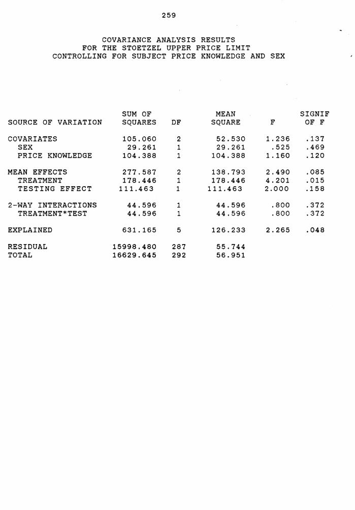
259

COVARIANCE ANALYSIS RESULTS FOR THE STOETZEL UP~ER PRICE LIMIT

CONTROLLING FOR SUBJECT PRICE KNOWLEDGE AND SEX

SUM OF MEAN SOURCE OF VARIATION SQUARES DF SQUARE F

COVARIATES 105.060 2 52.530 1.236 SEX 29.261 1 29.261 .525 PRICE KNOWLEDGE 104.388 1 104.388 1.160

MEAN EFFECTS 277.587 2 138.793 2.490 TREATMENT 178.446 1 178.446 4.201 TESTING EFFECT 111.463 1 111.463 2. 000

2-WAY INTERACTIONS 44.596 1 44.596 .800 TREATMENT* TEST 44.596 1 44.596 .800

EXPLAINED 631.165 5 126.233 2.265

RESIDUAL 15998.480 287 55.744 TOTAL 16629.645 292 56.951

SIGNIF OF F

.137

.469

.120

.085

.015

.158

.372

.372

.048

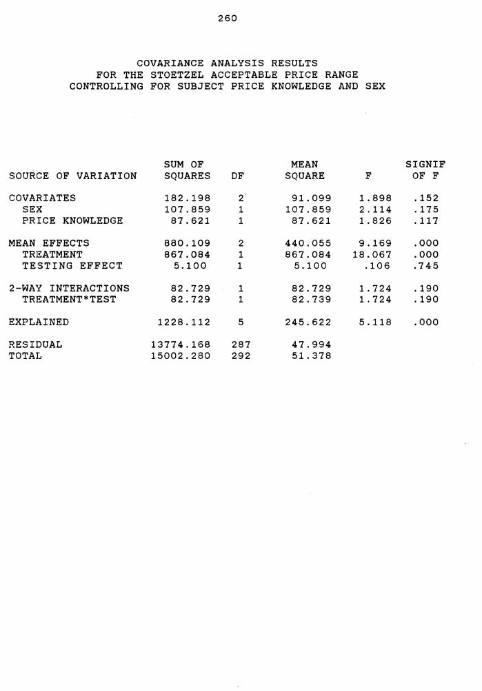
260

COVARIANCE ANALYSIS RESULTS FOR THE STOETZEL ACCEPTABLE PRICE RANGE

CONTROLLING FOR SUBJECT PRICE KNOWLEDGE AND SEX

SUM OF MEAN SOURCE OF VARIATION SQUARES DF SQUARE F

COVARIATES 182.198 2 91.099 1.898 SEX 107.859 1 107.859 2.114 PRICE KNOWLEDGE 87.621 1 87.621 1.826

MEAN EFFECTS 880.109 2 440.055 9.169 TREATMENT 867.084 1 867.084 18.067 TESTING EFFECT 5 .100 1 5 .100 .106

2-WAY INTERACTIONS 82.729 1 82.729 1.724 TRl~ATMENT*TEST 82.729 1 82.739 1.724

EXPLAINED 1228.112 5 245.622 5.118

RESIDUAL 13774.168 287 47.994 TOTAL 15002.280 292 51.378

SIGNIF OF F

.152

.175

.117

.000

.000

. 745

.190

.190

.000

261

COVARIANCE ANALYSIS RESULTS FOR THE OWN-CATEGORY LOWER PRICE LIMIT

CONTROLLING FOR SUBJECT PRICE KNOWLEDGE AND SEX

SUM OF MEAN SOURCE OF VARIATION SQUARES DF SQUARE F

COVARIATES 76.644 2 38.322 1.433 SEX 9.830 1 9.830 .367 PRICE KNOWLEDGE 51.297 1 51.297 1. 918

MEAN EFFECTS 385.232 2 192.616 7.200 TREATMENT 320.064 1 320.064 11. 964 TESTING EFFECT 74.577 1 74.577 2 .110

2-WAY INTERACTIONS 22.294 1 22.294 .833 TREATMENT*TEST 22.294 1 22.294 .833

EXPLAINED 555.004 5 111.001 4.149

RESIDUAL 6340.115 237 26.752 TOTAL 8695.119 242 28.492

SIGNIF OF F

.241

.545

.167

.001

.001

.12 6

.362

.362

.001

262

COVARIANCE ANALYSIS RESULTS FOR THE OWN-CATEGORY UPPER PRICE LIMIT

CONTROLLING FOR SUBJECT PRICE KNOWLEDGE AND SEX

SUM OF MEAN SOURCE OF VARIATION SQUARES DF SQUARE F

COVARIATES 242.853 2 121.427 1.818 SEX 98.640 1 98.640 1.476 PRICE KNOWLEDGE 123.947 1 123.947 1.855

MEAN EFFECTS 50.273 2 25.136 .376 TREATMENT 22.095 1 22.095 .331 TESTING EFFECT 29.753 1 29.753 . 445

2-WAY INTERACTIONS .634 1 .634 .009 TREATMENT*TEST .634 1 .634 .009

EXPLAINED 329.240 5 65.848 .986

RESIDUAL 15833.426 237 66.808 TOT Al~ 16162.667 242 66.788

SIGNIF OF F

.165

.422

.150

.687

.556

.505

.922

.922

.427

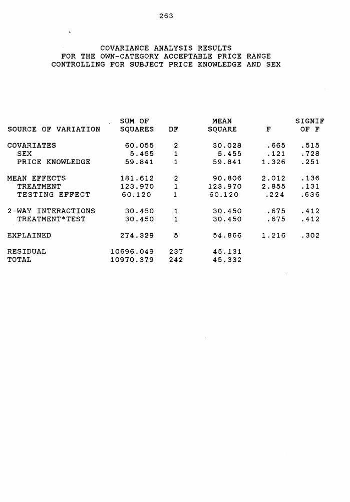
263

COVARIANCE ANALYSIS RESULTS FOR THE OWN-CATEGORY ACCEPTABLE PRICE RANGE

CONTROLLING FOR SUBJECT PRICE KNOWLEDGE AND SEX

SUM OF MEAN SOURCE OF VARIATION SQUARES DF SQUARE F

COVARIATES 60.055 2 30.028 .665 SEX 5.455 1 5.455 .121 PRICE KNOWLEDGE 59.841 1 59.841 1.326

MEAN EFFECTS 181.612 2 90.806 2.012 TREATMENT 123.970 1 123.970 2.855 TESTING EFFECT 60.120 1 60.120 . 2 2 4

2-WAY INTERACTIONS 30.450 1 30.450 .675 TREATMENT*TEST 30.450 1 30.450 .675

EXPLAINED 274.329 5 54.866 1.216

RESIDUAL 10696.049 237 45.131 TOT AI, 10970.379 242 45.332

SIGNIF OF F

.515

.728

.251

.136

.131

. 636

.412

.412

.302

The vita has been removed from the scanned document